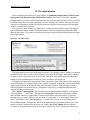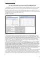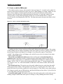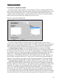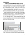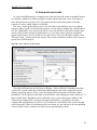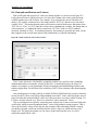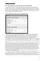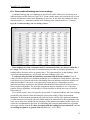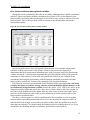
Download WarpPLS 1.0 User Manual

WarpPLS 3.0
User Manual
Ned Kock
WarpPLS 3.0 User Manual

WarpPLS 3.0
User Manual
Ned Kock
ScriptWarp Systems
Laredo, Texas
USA
ii
WarpPLS 3.0 User Manual
WarpPLS 3.0 User Manual, February 2012, Copyright  by Ned Kock
All rights reserved worldwide. No part of this publication may be reproduced or utilized in any
form, or by any means – electronic, mechanical, magnetic or otherwise – without permission in
writing from ScriptWarp Systems.
Software use agreement
The use of the software that is the subject of this manual (Sofware) requires a valid license,
which has a limited duration (usually no more than one year). Individual and organizational
licenses may be purchased from ScriptWarp Systems, or any authorized ScriptWarp Systems
reseller.
The Software is provided “as is”, and without any warranty of any kind. Free trial versions of the
Software are made available by ScriptWarp Systems with the goal of allowing users to assess,
for a limited time (usually one to three months), the usefulness of the Software for their data
modeling and analysis purposes. Users are strongly advised to take advantage of those free trial
versions, and ensure that the Software meets their needs before purchasing a license.
Free trial versions of the Software are full implementations of the software, minus the licenses.
That is, they are not demo versions. Nevertheless, they are provided for assessment purposes
only, and not for “production” purposes, such as to analyze data and subsequently publish it as a
consulting or research report. Users are expected to purchase licenses of the Software before they
use it for “production” purposes.
Multivariate statistical analysis software systems are inherently complex, sometimes yielding
results that are biased and disconnected with the reality of the phenomena being modeled. Users
are strongly cautioned against accepting the results provided by the Software without doublechecking those results against: past empirical results obtained by other means and/or with other
software, applicable theoretical models, and practical commonsense assumptions.
Under no circumstances is ScriptWarp Systems to be held liable for any damages caused by the
use of the Software. ScriptWarp Systems does not guarantee in any way that the Software will
meet the needs of its users.
For more information:
ScriptWarp Systems
P.O. Box 452428
Laredo, Texas, 78045
USA
www.scriptwarp.com
iii
WarpPLS 3.0 User Manual
Table of contents
A. SOFTWARE INSTALLATION AND UNINSTALLATION ............................................................................. 1
A.I. NEW FEATURES IN VERSION 3.0 .......................................................................................................................... 2
B. THE MAIN WINDOW........................................................................................................................................... 5
B.I. SAVE GROUPED DESCRIPTIVE STATISTICS ............................................................................................................ 8
B.II. VIEW OR CHANGE SETTINGS ............................................................................................................................. 10
B.III. ANALYSIS ALGORITHM ................................................................................................................................... 11
B.IV. RESAMPLING METHOD .................................................................................................................................... 12
B.V. RANGE RESTRICTION........................................................................................................................................ 14
B.V. RANKED DATA ................................................................................................................................................. 15
C. STEP 1: OPEN OR CREATE A PROJECT FILE TO SAVE YOUR WORK ............................................... 16
D. STEP 2: READ THE RAW DATA USED IN THE SEM ANALYSIS ............................................................ 18
E. STEP 3: PRE-PROCESS THE DATA FOR THE SEM ANALYSIS............................................................... 20
F. STEP 4: DEFINE THE VARIABLES AND LINKS IN THE SEM MODEL.................................................. 21
F.I. CREATE OR EDIT THE SEM MODEL .................................................................................................................... 22
F.II. CREATE OR EDIT LATENT VARIABLE ................................................................................................................. 25
G. STEP 5: PERFORM THE SEM ANALYSIS AND VIEW THE RESULTS................................................... 27
H. VIEW AND SAVE RESULTS............................................................................................................................. 29
H.I. VIEW GENERAL SEM ANALYSIS RESULTS ......................................................................................................... 30
H.II. VIEW PATH COEFFICIENTS AND P VALUES ........................................................................................................ 32
H.III. VIEW STANDARD ERRORS AND EFFECT SIZES FOR PATH COEFFICIENTS ........................................................... 33
H.IV. VIEW COMBINED LOADINGS AND CROSS-LOADINGS........................................................................................ 35
H.V. VIEW PATTERN LOADINGS AND CROSS-LOADINGS ........................................................................................... 37
H.VI. VIEW STRUCTURE LOADINGS AND CROSS-LOADINGS ...................................................................................... 38
H.VII. VIEW INDICATOR WEIGHTS ............................................................................................................................ 39
H.VIII. VIEW LATENT VARIABLE COEFFICIENTS ....................................................................................................... 41
H.IX. VIEW CORRELATIONS AMONG LATENT VARIABLES ......................................................................................... 43
H.X. VIEW BLOCK VARIANCE INFLATION FACTORS .................................................................................................. 45
H.XI. VIEW CORRELATIONS AMONG INDICATORS..................................................................................................... 46
H.XII. VIEW/PLOT LINEAR AND NONLINEAR RELATIONSHIPS AMONG LATENT VARIABLES ....................................... 47
H.XIII. VIEW INDIRECT AND TOTAL EFFECTS ............................................................................................................ 50
I. GLOSSARY............................................................................................................................................................ 51
J. REFERENCES ...................................................................................................................................................... 54
iv
WarpPLS 3.0 User Manual
A. Software installation and uninstallation
The software installs automatically from a self-extracting executable file. There are two
components to the software: the MATLAB Compiler Runtime, and the main software (i.e.,
WarpPLS). The first is a set of free-distribution MATLAB libraries with code that is called by
the main software. Because the MATLAB Compiler Runtime is used, you do not have to have
MATLAB (the main MATLAB program) installed on your computer to run WarpPLS.
Minimal and harmless changes to the operating system registry are made by the MATLAB
Compiler Runtime, which are easily reversed upon uninstallation. To uninstall, go the “Control
Panel”, click on “Add or Remove Programs” or “Programs and Features”, and uninstall the
MATLAB Compiler Runtime.
The MATLAB Compiler Runtime 7.14 is used in this version of WarpPLS. This is the same
MATLAB Compiler Runtime as the one used in version 2.0. The MATLAB Compiler Runtime
used in version 1.0 is a different one, and thus will not work properly with this version of
WarpPLS.
In most cases, previous versions of WarpPLS and of the MATLAB Compiler Runtime
may be retained on a user’s computer. Different versions of WarpPLS and of the MATLAB
Compiler Runtime generally do not interfere with one other.
To uninstall the main software program, simply delete the main software installation folder,
which is usually “C:\Program Files\WarpPLS 3.0” or “C:\Program Files (x86)\WarpPLS 3.0”,
unless you chose a different folder for the main software program during the installation process.
Then delete the shortcut created by the software from the desktop.
Both programs, the MATLAB Compiler Runtime and the main software, may be retained
without harm to your computer. They will not interfere with other programs; not even with
MATLAB (the main MATLAB program), if you have it installed on your computer.
1
WarpPLS 3.0 User Manual
A.i. New features in version 3.0
Addition of latent variables as indicators. Users now have the option of adding latent
variable scores to the set of standardized indicators used in an SEM analysis. This option is
useful in the removal of outliers, through the use of restricted ranges for latent variable scores,
particularly for outliers that are clearly visible on the plots depicting associations among latent
variables. This option is also useful in hierarchical analysis, where users define second-order
(and higher order) latent variables, and then conduct analyses with different models including
latent variables of different orders.
Blindfolding. Users now have the option of using a third resampling algorithm, namely
blindfolding, in addition to bootstrapping and jackknifing. Blindfolding is a resampling
algorithm that creates a number of resamples (a number that can be selected by the user), where
each resample has a certain number of rows replaced with the means of the respective columns.
The number of rows modified in this way in each resample equals the sample size divided by the
number of resamples. For example, if the sample size is 200 and the number of resamples
selected is 100, then each resample will have 2 rows modified. If a user chooses a number of
resamples that is greater than the sample size, the number of resamples is automatically set to the
sample size (as with jackknifing).
Effect sizes. Cohen’s (1988) f-squared effect size coefficients are now calculated and shown
for all path coefficients. These are calculated as the absolute values of the individual
contributions of the corresponding predictor latent variables to the R-square coefficients of the
criterion latent variable in each latent variable block. With these effect sizes users can ascertain
whether the effects indicated by path coefficients are small, medium, or large. The values usually
recommended are 0.02, 0.15, and 0.35; respectively (Cohen, 1988). Values below 0.02 suggest
effects that are too weak to be considered relevant from a practical point of view, even when the
corresponding P values are statistically significant; a situation that may occur with large sample
sizes.
Estimated collinearity. Collinearity is now estimated before the SEM analysis is run. When
collinearity appears to be too high, users are warned about it. A table with estimated latent
variable correlations is shown, allowing users to identify the possible offending latent variables.
If users so choose, they can proceed with the analysis anyway, but in most cases the full
collinearity measures will confirm that collinearity is too high in their models for the analysis
results to be considered credible.
Full collinearity VIFs. VIFs are now shown for all latent variables, separately from the VIFs
calculated for predictor latent variables in individual latent variable blocks. These new VIFs are
calculated based on a full collinearity test, which enables the identification of not only vertical
but also lateral collinearity, and allows for a test of collinearity involving all latent variables in a
model. Vertical, or classic, collinearity is predictor-predictor latent variable collinearity in
individual blocks. Lateral collinearity is a new term that refers to predictor-criterion latent
variable collinearity; a type of collinearity that can lead to particularly misleading results. Full
collinearity VIFs can also be used for common method (Lindell & Whitney, 2001) bias tests that
are more conservative than, and arguably superior to, the traditionally used tests relying on
exploratory factor analyses.
Incremental code optimization. At several points the code was optimized for speed, stability,
and coefficient estimation precision. This led to incremental gains in speed even as a significant
number of new features were added. Several of these new features required new and complex
calculations, mostly to generate coefficients that were not available before.
2
WarpPLS 3.0 User Manual
Indirect and total effects. Indirect and total effects are now calculated and shown, together
with the corresponding P values, standard errors, and effect sizes. The calculation of indirect and
total effects can be critical in the evaluation of downstream effects of latent variables that are
mediated by other latent variables, especially in complex models with multiple mediating effects
along concurrent paths. Indirect effects also allow for direct estimations, via resampling, of the P
values associated with mediating effects that have traditionally relied on non-automated and thus
time-consuming calculations based on linear (Preacher & Hayes, 2004) and nonlinear (Hayes &
Preacher, 2010) assumptions.
P values for all weights and loadings. P values are now shown for all weights and loadings,
including those associated with indicators that make up moderating variables. With these P
values, users can check whether moderating latent variables satisfy validity and reliability
criteria for either reflective or formative measurement. This can help users demonstrate validity
and reliability in hierarchical analyses involving moderating effects, where double, triple etc.
moderating effects are tested. For instance, moderating latent variables can be created, added to
the model as standardized indicators, and then their effects modeled as being moderated by other
latent variables; an example of double moderation.
Predictive validity. Stone-Geisser Q-squared coefficients (Geisser, 1974; Stone, 1974) are
now calculated and shown for each endogenous variable in an SEM model. The Q-squared
coefficient is a nonparametric measure traditionally calculated via blindfolding. It is used for the
assessment of the predictive validity (or relevance) associated with each latent variable block in
the model, through the endogenous latent variable that is the criterion variable in the block.
Sometimes referred to as a resampling analog of the R-squared, it is often similar in value to that
measure; even though, unlike the R-squared coefficient, the Q-squared coefficient can assume
negative values. Acceptable predictive validity in connection with an endogenous latent variable
is suggested by a Q-squared coefficient greater than zero.
Project files for previous versions. If a project file created with a previous version of the
software is open, the software automatically recognizes that and converts the file to the new
version. This takes placed even with project files where all of the five steps of the SEM analysis
were completed.
Ranked data. Users can now select an option to conduct their analyses with only ranked data,
whereby all the data is automatically ranked prior to the SEM analysis (the original data is
retained in unranked format). When data is ranked, typically the value distances that typify
outliers are significantly reduced, effectively eliminating outliers without any decrease in sample
size. Often some information is lost due to ranking – e.g., the distances among data points based
on answers on ratio scales. Thus a concomitant increase in collinearity may be observed, but
typically not to the point of threatening the credibility of the results. This option can be very
useful in assessments of whether the presence of outliers significantly affects path coefficients
and respective P values, especially when outliers are not believed to be due to measurement
error.
Restricted ranges. Users can now run their analyses with subsamples defined by a range
restriction variable, which may be standardized or unstandardized. This option is useful in multigroup analyses, whereby separate analyses are conducted for each subsample and the results then
compared with one another. One example would be a multi-country analysis, with each country
being treated as a subsample, but without separate datasets for each country having to be
provided as inputs. This range restriction feature is also useful in situations where outliers are
causing instability in a resample set, which can lead to abnormally high standard errors and thus
3
WarpPLS 3.0 User Manual
inflated P values. Users can remove outliers by restricting the values assumed by a variable to a
range that excludes the outliers, without having to modify and re-read a dataset.
Standard errors for all weights and loadings. Standard errors are now shown for all
loadings and weights. Among other purposes, these standard errors can be used in multi-group
analyses, with the same model but different subsamples. In these cases, users may want to
compare the measurement models to ascertain equivalence, using a multi-group comparison
technique such as the one documented by Keil et al. (2000), and thus ensure that any observed
differences in structural model coefficients are not due to measurement model differences.
VIFs for all indicators. VIFs are now shown for all indicators, including those associated
with moderating latent variables. With these VIFs, users can check whether moderating latent
variables satisfy criteria for formative measurement, in case they do not satisfy validity and
reliability criteria for reflective measurement. This can be particularly helpful in hierarchical
analyses involving moderating effects, where formative latent variables are frequently employed,
including cases where double, triple etc. moderating effects are tested. Here moderating latent
variables can be created, added to the model as standardized indicators, and then their effects
modeled as being moderated by other latent variables; with this process being repeated at
different levels.
4
WarpPLS 3.0 User Manual
B. The main window
Prior to displaying the software’s main window, a command prompt window is shown and
kept open for the duration of the SEM analysis session. Do not try to close this command
prompt window, because it will list warnings and error messages that will likely be very useful in
troubleshooting. Moreover, those warnings and error messages will indicate where in the source
code they are happening, which will help the software developer correct any possible problems
in future versions of the software.
The software’s main window (see Figure B.1) is where the SEM analysis starts. The top-left
part of the main window contains a brief description of the five steps through which the SEM
analysis takes place. The steps are executed by pressing each of the push buttons on the top-right
part of the window.
Figure B.1. The main window
The steps must be carried out in the proper sequence. For example, Step 5, which is to perform
the SEM analysis and view the results, cannot be carried out before Step 1 takes place, which is
to open or create a project file to save your work. Therefore, unavailable steps have their push
buttons grayed out and deactivated, until it is time for them to be carried out.
The bottom-left part of the main window shows the status of the SEM analysis; after each step
in the SEM analysis is completed, this status window is updated. A miniature version of the SEM
model graph is shown at the bottom-right part of the main window. This miniature version is
displayed without results after Step 4 is completed. After Step 5 is completed, this miniature
version is displayed with results.
The “Project” menu options. There are three project menu options available: “Save project”,
“Save project as …”, and “Exit”. Through the “Save project” option you can choose a folder
and file name, and save a project that is currently open or has just been created. To open an
existing project or create a new project you need to execute Step 1, by pressing the “Proceed to
Step 1” push button. The “Save project as …” option allows you to save an existing project
with a different name. This option is useful in the SEM analysis of multiple models where each
model is a small variation of the previous one. Finally, the “Exit” option ends the software
session. If your project has not been saved, and you choose the “Exit” option, the software will
5
WarpPLS 3.0 User Manual
ask you if you want to save your project before exiting. In some cases, you will not want to save
your project before exiting, which is why a project is not automatically saved after each step is
completed. For example, you may want to open an existing project, change a few things and then
run an SEM analysis, and then discard that project. You can do this by simply not saving the
project before exiting.
The “Settings” menu option. You can view or change general SEM analysis settings through
the “Settings” menu option. Here you can select the analysis algorithm used in the SEM analysis,
the resampling method used to calculate standard errors and P values, as well as other elements
that will define how the SEM analysis will be conducted. This menu option is discussed in more
detail later.
The “Help” menu options. There are several help menu options available on the main
window, as well as on several other windows displayed by the software. The “Open help file for
this window (PDF)” option opens a PDF file with help topics that are context-specific, in this
case specific to the main window. The “Open User Manual file (PDF)” option opens this
document, and is not context-specific. The “Open Web page with video for this window”
option opens a Web page with a video clip that is context-specific, in which case specific to the
main window. The “Open Web page with links to various videos” option is not contextspecific, and opens a Web page with links to various video clips. The “Open Web page with
WarpPLS blog” option opens a Web page with the WarpPLS blog.
The “Data” menu options. After Step 3 is completed, whereby the data used in the SEM
analysis is pre-processed, seven data menu options become available (see Figure B.2). These
menu options allow you to view or save data into tab-delimited .txt files. The “tab-delimited .txt
file” is the general file format used by the software to save most of the files containing analysis
and summarization results. These files can be opened and edited using Excel, Notepad, and other
similar spreadsheet or text editing software.
Figure B.2. Save menu options on main window (available after Step 3 only)
The “View or save indicator correlations, means and standard deviations” option allows
you to save general descriptive statistics about the data, which are complemented by the option
“View or save P values for indicator correlations”.
Two menu options allow you to save unstandardized pre-processed indicator data. These
options are: “View or save unstandardized pre-processed indicator data” and “View or save
unstandardized ranked pre-processed indicator data”. The latter option refers to ranked data.
When data is ranked, typically the value distances that typify outliers in data on ratio scales,
whether standardized or unstandardized, are significantly reduced. This effectively eliminates
outliers from the data, without any decrease in sample size. Often some information is lost due to
ranking – e.g., the distances among data points based on answers on ratio scales.
6
WarpPLS 3.0 User Manual
Two related menu options allow you to save standardized pre-processed indicator data: “View
or save standardized pre-processed indicator data” and “View or save standardized ranked
pre-processed indicator data”. The latter option ranks the data prior to standardizing it.
The options that refer to unstandardized data allow you to view and save pre-processed data
prior to standardization. The options that refer to standardized data allow you to view and save
pre-processed data after standardization; that is, after all indicators have been transformed in
such a way that they have a mean of zero and a standard deviation of one.
The “Save grouped descriptive statistics” option is a special option that allows you to save
descriptive statistics (means and standard deviations) organized by groups defined based on
certain parameters; this option is discussed in more detail below.
7
WarpPLS 3.0 User Manual
B.i. Save grouped descriptive statistics
When the “Save grouped descriptive statistics” option is selected, a data entry window is
displayed (see Figure B.3). There you can choose a grouping variable, number of groups, and the
variables to be grouped. This option is useful if one wants to conduct a comparison of means
analysis using the software, where one variable (the grouping variable) is the predictor, and one
or more variables are the criteria (the variables to be grouped).
Figure B.3. Save grouped descriptive statistics window
Figure B.4 shows the grouped statistics data saved through the window shown in Figure B.3.
The tab-delimited .txt file was opened with a spreadsheet program, and contained the data on the
left part of the figure.
Figure B.4. Grouped descriptive statistics bar chart
That data on the left part of Figure B.4 was organized as shown above the bar chart; next the
bar chart was created using the spreadsheet program’s charting feature. If a simple comparison of
8
WarpPLS 3.0 User Manual
means analysis using this software had been conducted in which the grouping variable (in this
case, an indicator called “ECU1”) was the predictor, and the criterion was the indicator called
“Effe1”, those two variables would have been connected through a path in a simple path model
with only one path. Assuming that the path coefficient was statistically significant, the bar chart
displayed in Figure B.4, or a similar bar chart, could be added to a report describing the analysis.
Some may think that it is an overkill to conduct a comparison of means analysis using an SEM
software package such as this, but there are advantages in doing so. One of those advantages is
that this software calculates P values using a nonparametric class of estimation techniques,
namely resampling estimation techniques. (These are sometimes referred to as bootstrapping
techniques, which may lead to confusion since bootstrapping is also the name of a type of
resampling technique.) Nonparametric estimation techniques do not require the data to be
normally distributed, which is a requirement of other comparison of means techniques (e.g.,
ANOVA).
Another advantage of conducting a comparison of means analysis using this software is that
the analysis can be significantly more elaborate. For example, the analysis may include control
variables (or covariates), which would make it equivalent to an ANCOVA test. Finally, the
comparison of means analysis may include latent variables, as either predictors or criteria. This is
not usually possible with ANOVA or commonly used nonparametric comparison of means tests
(e.g., the Mann-Whitney U test).
9
WarpPLS 3.0 User Manual
B.ii. View or change settings
The view or change settings window (see Figure B.5) allows you to: select an algorithm for
the SEM analysis; select a resampling method; select the number of resamples used, if the
resampling method selected was bootstrapping or blindfolding; select a range restriction variable
type; select a range restriction variable; select a range, in the form of minimum and maximum
values, for the range restriction variable; and choose whether to use only ranked data in the
analysis or not.
Figure B.5. View or change settings window
The following subsections provide more details on the options available on the view or change
settings window. The settings chosen for each of the options can have a dramatic effect on
the results of a SEM analysis. As such, they should be used with caution, and normally after a
new project file (with a unique name) is created and the previous one saved, so that users can
revert back to project files with previously selected settings. At the same time, the right
combinations of settings can provide major insights into the data being analyzed.
10
WarpPLS 3.0 User Manual
B.iii. Analysis algorithm
Many relationships in nature, including relationships involving behavioral variables, are
nonlinear and follow a pattern known as U-curve (or inverted U-curve). In this pattern a variable
affects another in a way that leads to a maximum or minimum value, where the effect is either
maximized or minimized, respectively. This type of relationship is also referred to as a J-curve
pattern; a term that is more commonly used in economics and the health sciences.
The term “U-curve” is used here also to refer to nonlinear relationships that can be
represented as sections of a U curve. As such, it covers all noncyclical nonlinear relationships.
These relationships include the logarithmic, hyperbolic decay, exponential decay,
exponential, and quadratic relationships, among others. That is, these relationships can be
conceptually modeled as variations of U-curve relationships.
The analysis algorithms available are Warp3 PLS Regression, Warp2 PLS Regression, PLS
Regression, and Robust Path Analysis. The Warp2 PLS Regression algorithm tries to identify a
U-curve relationship between latent variables, and, if that relationship exists, the algorithm
transforms (or “warps”) the scores of the predictor latent variables so as to better reflect the Ucurve relationship in the estimated path coefficients in the model.
The Warp3 PLS Regression algorithm, the default algorithm used by the software, tries to
identify a relationship between latent variables defined by a function whose first derivative is a
U-curve. This type of relationship follows a pattern that is more similar to an S-curve (or a
somewhat distorted S-curve), and can be seen as a combination of two connected U-curves, one
of which is inverted.
The PLS Regression algorithm does not perform any warping of relationships. It is
essentially a standard PLS regression algorithm, whereby indicators’ weights, loadings and
factor scores (a.k.a. latent variable scores) are calculated based on an algorithm that maximizes
the variance explained in the latent variable scores by the latent variable indicators, after which
path coefficients are estimated using a robust path analysis algorithm.
A key criterion for the calculation of the weights, observed in virtually all PLS-based
algorithms, is that the regression equation expressing the relationship between the indicators and
the factor scores has an error term that equals zero. In other words, the factor scores are
calculated as exact linear combinations of their indicators. PLS regression is the underlying
weight calculation algorithm used in both Warp3 and Warp2 PLS Regression.
The warping takes place during the estimation of path coefficients, and after the estimation of
all weights and loadings in the model. The weights and loadings of a model with latent variables
make up what is often referred to as the outer model (a.k.a. measurement model), whereas the
path coefficients among latent variables make up what is often called the inner model (a.k.a.
structural model).
Finally, the Robust Path Analysis algorithm is a simplified algorithm in which factor scores
are calculated by averaging all of the indicators associated with a latent variable; that is, in this
algorithm weights are not estimated through PLS regression. This algorithm is called “Robust”
Path Analysis, because, as with most robust statistics methods, the P values are calculated
through resampling. If all latent variables are measured with single indicators, the Robust Path
Analysis and the PLS Regression algorithms will yield identical results.
11
WarpPLS 3.0 User Manual
B.iv. Resampling method
One of a few resampling methods may be selected: bootstrapping, jackknifing, and
blindfolding. Bootstrapping, the software’s default, employs a resampling algorithm that creates
a number of resamples (a number that can be selected by the user), by a method known as
“resampling with replacement”. This means that each resample contains a random arrangement
of the rows of the original dataset, where some rows may be repeated. (The commonly used
analogy of a deck of cards being reshuffled, leading to many resample decks, is a good one; but
not entirely correct because in bootstrapping the same card may appear more than once in each
of the resample decks.)
Jackknifing, on the other hand, creates a number of resamples that equals the original sample
size, and each resample has one row removed. That is, the sample size of each resample is the
original sample size minus 1. Thus, when jackknifing is selected the number of resamples is
automatically set as the sample size.
Blindfolding employs a resampling algorithm that creates a number of resamples (a number
that can be selected by the user) by a method whereby each resample has a certain number of
rows replaced with the means of the respective columns. The number of rows modified in this
way in each resample equals the sample size divided by the number of resamples. For example,
if the sample size is 200 and the number of resamples selected is 100, then each resample will
have 2 rows modified. If a user chooses a number of resamples that is greater than the sample
size, the number of resamples is automatically set to the sample size (as with jackknifing).
The default number of resamples for bootstrapping and blindfolding is 100. It can be
modified by entering a different number in the appropriate edit box. (Please note that we are
talking about the number of resamples here, not the original data sample size.) Leaving the
number of resamples for bootstrapping as 100 is recommended because it has been shown
that higher numbers of resamples lead to negligible improvements in the reliability of P values;
in fact, even setting the number of resamples at 50 is likely to lead to fairly reliable P value
estimates (Efron et al., 2004).
Conversely, increasing the number of resamples well beyond 100 leads to a higher
computation load on the software, making the software look like it is having a hard time coming
up with the results. In very complex models, a high number of resamples may make the software
run very slowly.
Some researchers have suggested in the past that a large number of resamples can address
problems with the data, such as the presence of outliers due to errors in data collection. This
opinion is not shared by the original developer of the bootstrapping method, Bradley Efron (see,
e.g., Efron et al., 2004).
Arguably jackknifing is particularly good at addressing problems associated with the presence
of outliers due to errors in data collection. Generally speaking, jackknifing tends to generate
more stable resample path coefficients (and thus more reliable P values) with small sample
sizes (lower than 100), and with samples containing outliers (see, e.g., Chiquoine &
Hjalmarsson, 2009).
Bootstrapping tends to generate more stable resample path coefficients (and thus more
reliable P values) with larger samples and with samples where the data points are evenly
distributed on a scatter plot. The use of bootstrapping with small sample sizes (lower than 100)
has been discouraged (Nevitt & Hancock, 2001).
Bootstrapping and jackknifing can be seen as complementary resampling methods, in that one
tends to perform well in situations where the other does not, and vice-versa.
12
WarpPLS 3.0 User Manual
Blindfolding tends to perform somewhere in between jackknifing and bootstrapping. If
the number of resamples is set as very close to the sample size, particularly with small sample
sizes (lower than 100) and with samples containing outliers, blindfolding performs similarly to
jackknifing. With larger samples and with samples where the data points are evenly distributed
on a scatter plot, blindfolding tends to performs more like bootstrapping, especially when the
number of resamples is set as the same for both algorithms.
Since the warping algorithms are also sensitive to the presence of outliers, in many cases it
is a good idea to estimate P values with both bootstrapping and jackknifing, which are
complementary resampling methods, and use the P values associated with the most stable
coefficients. An indication of instability is a high P value (i.e., statistically non-significant)
associated with path coefficients that could be reasonably expected to have low P values. For
example, with a sample size of 100, a path coefficient of 0.2 could be reasonably expected to
yield a P value that is statistically significant at the 0.05 level. If that is not the case, there may be
a stability problem. Another indication of instability is a marked difference between the P values
estimated through bootstrapping and jackknifing.
P values can be easily estimated using two or more resampling methods by following this
simple procedure. Run an SEM analysis of the desired model, using one of the resampling
methods, and save the project. Then save the project again, this time with a different name,
change the resampling method, and run the SEM analysis again. Then save the second project
again. Each project file will now have results that refer to one of the resampling methods. The P
values can then be compared, and the most stable ones used in a research report on the SEM
analysis. While this is a perfectly valid approach for the calculation of P values, as the
coefficients to which the P values refer do not change across iterations, it is very important to
fully disclose this to the readers of the research report.
13
WarpPLS 3.0 User Manual
B.v. Range restriction
Users can run their analyses with subsamples defined by a range restriction variable, which
is chosen from among the indicators available. (After Step 5 is completed, latent variable scores
can also be added to the model as standardized indicators.)
Two range restriction variable types are available: standardized and unstandardized
indicators. This means that the range restriction variable can be either a standardized or
unstandardized indicator. Once a range restriction variable is selected, minimum and
maximum values must be set (i.e., a range), which in turn has the effect of restricting the
analysis to the rows in the dataset within that particular range.
The option of selecting a range restriction variable and respective range is useful in multigroup analyses, whereby separate analyses are conducted for group-specific subsamples, saved
as different project files, and the results then compared against one another. One example would
be a multi-country analysis, with each country being treated as a subsample, but without separate
datasets for each country having to be provided as inputs.
Let us assume that an unstandardized variable called “Country” stores the values “1” (for
Brazil), “2” (for New Zealand), and “3” (for the USA). To run the analysis only with data from
Brazil one can set the range restriction variable as “Country” (after setting its type as
“Unstandardized indicator”), and then set both the minimum and maximum values as “1” for the
range.
This range restriction feature is also useful in situations where outliers are causing instability
in a resample set, which can lead to abnormally high standard errors and thus inflated P values.
Users can remove outliers by restricting the values assumed by a variable to a range that
excludes the outliers, without having to modify and re-read a dataset.
14
WarpPLS 3.0 User Manual
B.v. Ranked data
Users can select an option to conduct their analyses with only ranked data, whereby all of the
data is automatically ranked prior to the SEM analysis (the original data is retained in unranked
format). When data is ranked, typically the value distances that typify outliers are significantly
reduced, effectively eliminating outliers without any decrease in sample size. This cannot be
achieved through standardization only.
Often some information is lost due to ranking – e.g., the distances among data points based on
answers on ratio scales. Thus a concomitant increase in collinearity may be observed, but
typically not to the point of threatening the credibility of the results. The option of using only
ranked data in the analysis can be very useful in assessments of whether the presence of outliers
significantly affects path coefficients and respective P values, especially when outliers are not
believed to be due to measurement error.
15
WarpPLS 3.0 User Manual
C. Step 1: Open or create a project file to save your work
Through Step 1, you will open or create a project file to save your work (see Figure C.1).
Project files are saved with the “.prj” extension, and contain all of the elements needed to
perform an SEM analysis. That is, they contain the original data used in the analysis, the
graphical model, the inner and outer model structures, and the results.
Figure C.1. Step 1 window
Once an original data file is read into a project file, the original data file can be deleted
without effect on the project file. The project file will store the original location and file name of
the data file, but it will no longer use it.
Project files may be created with one name, and then renamed using Windows Explorer or
another file management tool. Upon reading a project file that has been renamed in this fashion,
the software will detect that the original name is different from the file name, and will adjust
accordingly the name of the project file that it stores internally.
Different users of this software can easily exchange project files electronically if they are
collaborating on a SEM analysis project. This way they will have access to all of the original
data, intermediate data, and SEM analysis results in one single file. Project files are relatively
small. For example, a complete project file of a model containing 5 latent variables, 32 indicators
(columns in the original dataset), and 300 cases (rows in the original dataset) will typically be
only approximately 200 KB in size. Simpler models may be stored in project files as small as 50
KB.
If a project file created with a previous version of the software is open, the software
automatically recognizes that and converts the file to the new version. This takes placed even
with project files where all of the five steps of the SEM analysis were completed. However,
because each new version incorporates new features, with outputs stored within new or modified
software objects, normally previous versions of the software cannot properly reuse project
files created with more recent versions.
16
WarpPLS 3.0 User Manual
17
WarpPLS 3.0 User Manual
D. Step 2: Read the raw data used in the SEM analysis
Through Step 2, you will read the raw data used in the SEM analysis (see Figure D.1). While
this should be a relatively trivial step, it is in fact one of the steps where users have the most
problems with other SEM software. Often an SEM software application will abort, or freeze, if
the raw data is not in the exact format required by the SEM software, or if there are any problems
with the data, such as missing values (empty cells).
Figure D.1. Step 2 window
This software employs an import wizard that avoids most data reading problems, even if it
does not entirely eliminate the possibility that a problem will occur. Click only on the “Next”
and “Finish” buttons of the file import wizard, and let the wizard do the rest. Soon after the
raw data is imported, it will be shown on the screen, and you will be given the opportunity to
accept or reject it. If there are problems with the data, such as missing column names, simply
click “No” when asked if the data looks correct.
Raw data can be read directly from Excel files, with extensions “.xls” or “.xlsx”, or text files
where the data is tab-delimited or comma-delimited. When reading from an “.xls” or “.xlsx”
file that contains a workbook with multiple worksheets, make sure that the worksheet that
contains the data is the first on the workbook. If the workbook has multiple worksheets, the
file import wizard used in Step 2 will typically select the first worksheet as the source or raw
data. Raw data files, whether Excel or text files, must have indicator names in the first row,
and numeric data in the following rows. They may contain empty cells, or missing values;
these will be automatically replaced with column averages in a later step.
Users may want to employ different approaches to handle missing values, such as deleting the
rows where they appear, or manually replacing them with the average of nearby values on the
same column. The most widely used approach, and also generally the most reliable, is replacing
the missing values with column averages. While this is done automatically by the software, you
18
WarpPLS 3.0 User Manual
should not use datasets with too many missing values, as this will distort the results. A general
rule of thumb is that your dataset should not have any column with more than 10 percent
of its values missing; a more relaxed rule would be to set the threshold to 20 percent (Hair
et al., 1987; 2009). One can reduce the percentage of missing values per column by deleting
rows in the dataset, where the deleted rows are the ones that refer to the columns with missing
values.
One simple test can be used to try to find out if there are problems with a raw data file. Try to
open it with a spreadsheet software (e.g., Excel), if it is originally a text file; or to try to create a
tab-delimited text file with it, if it is originally a spreadsheet file. If you try to do either of these
things, and the data looks corrupted (e.g., missing column names, with misplaced columns,
containing unrecognized symbols), then it is likely that the original file has problems, which may
be hidden from view. For example, a spreadsheet file may be corrupted, but that may not be
evident based on a simple visual inspection of the contents of the file.
19
WarpPLS 3.0 User Manual
E. Step 3: Pre-process the data for the SEM analysis
In Step 3 the raw data will be pre-processed for the SEM analysis. This is mostly an automatic
process, requiring only a few button clicks from you. This step will correct problems with the
data, such as identical column names, columns with zero variance, and missing values.
This step will also let you know if the data has rank problems, which usually happens when
the sample size is very small relative to the number of existing indicators. A related cause of rank
problems is a sample with many repeated or linearly dependent values on different rows or
columns, which sometimes is an indication of data fabrication. Please note that the term “rank”
here comes from matrix algebra, and is unrelated to the same term used in the context of ranked
data, as discussed earlier in connection with the software settings.
If there are rank problems, that does not mean that you cannot proceed with the SEM analysis,
but the results may be unstable and, in some cases, completely unreliable. It is not uncommon for
rank problems to be reported, and the results of the ensuing SEM analysis still remain reliable.
This is due to the general robustness of PLS-based methods for SEM analysis.
At the end of this step, a window will be displayed with the pre-processed data, which will be
standardized. Standardized data columns have means that equal zero and standard
deviations that equal one. Previously missing values will be shown as zero, since they were
replaced with the averages (or means) of the columns. Standardized data usually ranges from
-4 to 4, with outliers usually assuming values toward the left or right end of those extremes,
sometimes beyond -4 or 4.
Outliers can significantly change the shape of a nonlinear relationship, but this may also be the
case with linear relationships. For example, one single outlier may change the sign of a linear
relationship, from positive to negative (i.e., changing the association from direct to inverse).
Because of this, there is invariably the temptation of removing outliers from analyses. This is
often a mistake (Giaquinta, 2009; Hair et al., 2009), as outliers can be invaluable in elucidating
the true nature of an association (Kaiser, 2010; Rosenthal & Rosnow, 1991; Wold et al., 2001).
Generally speaking, outliers should only be removed if it is apparent that they are due to data
collection error.
After the software displays the pre-processed and standardized data, typically you will accept
the data and move on to the next step. If the data looks corrupted, do not accept it; click on the
“No” button when asked if the data looks correct. If there are problems in this step, they will
usually be related to problems with the raw data file. Check that file, and see if you can correct
those problems.
As mentioned before in this manual, one simple test can be used to try to find out if there are
problems with a raw data file. Try to open it with a spreadsheet program, if it is originally a text
file; or to try to create a tab-delimited text file with it, if it is originally a spreadsheet file. If you
try to do either of these things, and the data looks “messed up” (e.g., corrupted, or missing
column names), then it is likely that the original file has problems, which may be hidden from
view. For example, a spreadsheet file may be corrupted, but that may not be evident based on a
simple visual inspection of the contents of the file using spreadsheet software.
20
WarpPLS 3.0 User Manual
F. Step 4: Define the variables and links in the SEM model
In Step 4 you will define the latent variables and links in the SEM model. You will define the
latent variables by selecting the indicators that are associated with them, and the measurement
method used – either formative or reflective. The process of defining the latent variables in an
SEM model in this fashion is often called “defining the outer model”, in SEM lingo.
Model links can be of two types, direct and moderating links. Direct links connect pairs of
latent variables. Moderating links connect latent variables and direct links; that is, they refer to
effects in which a latent variable moderates the relationship between a pair of latent variables.
The process of defining model links is often referred to as “defining the inner model”.
21
WarpPLS 3.0 User Manual
F.i. Create or edit the SEM model
The window used to create or edit a model is shown in Figure F.1. A model can be edited if it
has been created and saved before as part of a project. While editing or creating a model you can
choose from a number of menu options related to overall model functions, latent variable
functions, direct link functions, and moderating link functions. As with other windows in this
software, there is a help menu option that provides access to this manual and to a contextspecific help file; both displayed as PDF files. The help menu option also provides links to Web
resources.
Figure F.1. Create or edit the SEM model window
A guiding text box is shown at the top of the model editing and creation window. The content
of this guiding text box changes depending on the menu option you choose, guiding you through
the sub-steps related to each option. For example, if you choose the option “Create latent
variable”, the guiding text box will change color, and tell you to select a location for the latent
variable on the model graph.
Direct links are displayed as full arrows in the model graph, and moderating links as
dashed arrows. Each latent variable is displayed in the model graph within an oval symbol,
where its name is shown above a combination of alphanumerical characters with this general
format: “(F)16i”. The “F” refers to the measurement model; where “F” means formative, and
“R” reflective. The “16i” reflects the number of indicators of the latent variable, which in this
case is 16.
Save model and close. This option saves the model within the project, and closes the model
editing and creation window. This option does not, however, save the project file. That is, the
project file has to be saved for a model to be saved as part of it. This allows you to open a project
file, change its model, run an SEM analysis, and discard all that you have done, if you wish to do
so, reverting back to the previous project file.
Centralize model graph. This option centralizes the model graph, and is useful when you are
building complex models and, in the process of doing so, end up making the model visually
22
WarpPLS 3.0 User Manual
unbalanced. For example, you may move variables around so that they are all accidentally
concentrated on the left part of the screen. This option corrects that by automatically redrawing
all symbols in the model graph so that the center of the model graph coincides with the center of
the model screen.
Show/hide indicators. This option shows or hides the list of indicators for each latent
variable. The indicators are shown on a vertical list next to each latent variable, and without the
little boxes that are usually shown in other SEM software. This display option is used to give the
model graph a cleaner look. It also has the advantage that it saves space in the model graph for
latent variables. Normally you will want to keep the indicators hidden, except when you are
checking whether the right indicators were selected for the right latent variables. That is,
normally you will show the indicators to perform a check, and then hide them during most of the
model building process.
Clear model (deletes all latent variables). This option deletes all latent variables, essentially
clearing the model. Given that choosing this option by mistake can potentially cause some
serious loss of work (not to mention some major user aggravation), the software shows a dialog
box asking you to confirm that you want to clear the model before it goes ahead and deletes all
latent variables. Even if you choose this option by mistake, and confirm your choice also by
mistake (a double mistake), you can still undo it by choosing the option “Cancel model
creation/editing (all editing is lost)” immediately after clearing the model.
Cancel model creation/editing (all editing is lost). This option cancels the model creation or
editing, essentially undoing all of the model changes you have made.
Save model into .jpg file. This option allows you to save the model into a .jpg file. You will
be asked to select the file name and the folder where the file will be saved. After saved, this file
can then be viewed and edited with standard picture viewers, as well as included as a picture into
other files (e.g., a Word file).
Create latent variable. This option allows you to create a latent variable, and is discussed in
more detail below. Once a latent variable is created it can be dragged and dropped anywhere
within the window that contains the model.
Edit latent variable. This option allows you to edit a latent variable that has already been
created, and thus that is visible on the model graph.
Delete latent variable. This option allows you to delete an existing latent variable. All links
associated with the latent variable are also deleted.
Move latent variable. This option is rarely used since, once a latent variable is created, it can
be easily dragged and dropped with the pointing device (e.g., mouse) anywhere within the
window that contains the model. This option is a carryover from a previous version, maintained
for consistency and for those users who still want to use it. It allows a user to move a latent
variable across the model by first clicking on the variable and then on the destination position.
Create direct link. This option allows you to create a direct link between one latent variable
and another. The arrow representing the link points from the predictor latent variable to the
criterion latent variable. Direct links are usually associated with direct cause-effect hypotheses;
testing a direct link’s strength (through the calculation of a path coefficient) and statistical
significance (through the calculation of a P value) equals testing a direct cause-effect hypothesis.
Delete direct link. This option allows you to delete an existing direct link. You will click on
the direct link that you want to delete, after which the link will be deleted.
Create moderating link. This option allows you to create a link between a latent variable and
a direct link. Given that the underlying algorithm used for outer model estimation is PLS
23
WarpPLS 3.0 User Manual
regression, both formative and reflective latent variables can be part of moderating links. This is
not possible with some variations of the PLS regression algorithm, often defined by “modes”
(see Lohmöller, 1989), which are implemented through other PLS-based SEM software tools.
Moderating links are usually associated with moderating cause-effect hypotheses, or interaction
effect hypotheses; testing a moderating link’s strength (through the calculation of a path
coefficient) and statistical significance (through the calculation of a P value) equals testing a
moderating cause-effect or interaction effect hypothesis. Moderating links should be used with
moderation (no pun intended), because they may introduce multicollinearity into the model,
and also because they tend to add nonlinearity to the model, and thus may make some model
parameter estimates unstable.
Delete moderating link. This option allows you to delete an existing moderating link. You
will click on the moderating link that you want to delete, after which the link will be deleted.
After you create a model and choose the option “Save model and close” a wait bar will be
displayed on the screen telling you that the SEM model structure is being created. This is an
important sub-step where a number of checks are made. In this sub-step, if there are any
moderating links in the model, new latent variables are created to store information about those
moderating effects using a procedure described and validated by Chin et al. (2003). The more
moderating links there are in a model, the longer this sub-step will take. In models where only
reflective variables are involved in a moderating link, typically this sub-step will not take longer
than a few seconds. Moderating links with formative variables may lead to longer wait times,
because formative variables are usually more complex, with significantly more indicators than
reflective variables.
24
WarpPLS 3.0 User Manual
F.ii. Create or edit latent variable
The latent variable creation window is show in Figure F.2, and it is virtually identical to the
latent variable editing window. The latent variable will appear in the model graph as soon as you
click on the menu option under “Save”, which saves the latent variable and closes the latent
variable creation or editing window. A latent variable is not saved as part of a project until the
model is saved as part of the project, and the project file is saved.
Figure F.2. Create latent variable window
You create a latent variable by entering a name for it, which may have no more than 8
characters, but to which no other restrictions apply. The latent variable name may contain letters,
numbers, and even special characters such as “@” or “$”. Then you select the indicators that
make up the latent variable, and define the measurement model as reflective or formative.
A reflective latent variable is one in which all the indicators are expected to be highly
correlated with the latent variable score. For example, the answers to certain question-statements
by a group of people, measured on a 1 to 7 scale (1=strongly disagree; 7=strongly agree) and
answered after a meal, are expected to be highly correlated with the latent variable “satisfaction
with a meal”. Among question-statements that would arguably fit this definition are the
following two: “I am satisfied with this meal”, and “After this meal, I feel full”. Therefore, the
latent variable “satisfaction with a meal”, can be said to be reflectively measured through two
indicators. Those indicators store answers to the two question-statements. This latent variable
could be represented in a model graph as “Satisf”, and the indicators as “Satisf1” and “Satisf2”.
A formative latent variable is one in which the indicators are expected to measure certain
attributes of the latent variable, but the indicators are not expected to be highly correlated with
the latent variable score, because they (i.e., the indicators) are not expected to be correlated with
each other. For example, let us assume that the latent variable “Satisf” (“satisfaction with a
meal”) is now measured using the two following question-statements: “I am satisfied with the
main course” and “I am satisfied with the dessert”. Here, the meal comprises the main course,
say, filet mignon; and a dessert, a fruit salad. Both main course and dessert make up the meal
(i.e., they are part of the same meal) but their satisfaction indicators are not expected to be highly
correlated with each other. The reason is that some people may like the main course very much,
25
WarpPLS 3.0 User Manual
and not like the dessert. Conversely, other people may be vegetarians and hate the main course,
but may like the dessert very much.
If the indicators are not expected to be highly correlated with each other, they cannot be
expected to be highly correlated with their latent variable’s score. So here is a general rule of
thumb that can be used to decide if a latent variable is reflectively or formatively measured. If
the indicators are expected to be highly correlated, then the measurement model should be set as
reflective. If the indicators are not expected to be highly correlated, even though they clearly
refer to the same latent variable, then the measurement model should be set as formative.
26
WarpPLS 3.0 User Manual
G. Step 5: Perform the SEM analysis and view the results
Step 5 performs the SEM analysis based on the model created in Step 4. After you click on the
button to perform the SEM analysis, the software will show a wait bar. This wait bar will update
you on the progress of the SEM analysis, which usually will take only a few seconds for simple
to moderately complex models. As soon as the SEM analysis is completed, the software will
show the results in graphical format on a window. That window also has menu options that allow
you to view more details about the results, including some that are not shown on the graph (e.g.,
reliability measures), and also save the results into tab-delimited text files.
Collinearity is estimated before the SEM analysis is run. When collinearity appears to be
too high, users are warned about it. A table with estimated latent variable correlations is shown,
allowing users to identify the possible offending latent variables. If users so choose, they can
proceed with the analysis anyway, but in most cases the full collinearity measures will confirm
that collinearity is too high in their models for the analysis results to be considered credible.
Once Step 5 is completed, two new options become available from the main window. One of
the new options is actually a sub-option under the “Data” menu option (which becomes available
after Step 3 is completed); this new sub-option allows users to save latent variable (a.k.a. factor)
scores. This option is provided on the main window for completeness, as it is also available
under the “Save” menu option on the results window.
The other new option that becomes available from the main window after Step 5 is completed
is the “Modify” menu option (see Figure G.1). This option allows users to add one or more latent
variable scores to the model as new standardized indicators, and also to add all latent variable
scores as new indicators. Adding one or more latent variable scores at a time may be advisable in
certain cases, as in hierarchical analyses using selected latent variable scores as indicators at each
level. In such cases, adding all latent variable scores at once may soon clutter the set of
indicators available to be used in the SEM model.
Figure G.1. New main window option available after Step 5 is completed
The option of adding latent variable scores to the model as new standardized indicators is
useful in the removal of outliers, through the use of restricted ranges for latent variable scores,
particularly for outliers that are clearly visible on the plots depicting associations among latent
variables. As briefly mentioned earlier, this option is also useful in hierarchical analysis, where
27
WarpPLS 3.0 User Manual
users define second-order (and higher order) latent variables, and then conduct analyses with
different models including latent variables of different orders.
This software uses algorithms that are fairly computing intensive, in some cases employing
multiple checks and optimization sub-algorithms in each sub-step. Therefore the speed with
which the analysis is conducted is a little slower than that of some other publicly available SEM
software. The differences in speed are not significant though, and normally the results generated
by this software are more complete, and in many cases more reliable. For example, this software
calculates model fit indices, as well as P values for most of its parameter estimates. Publicly
available PLS-based SEM software usually do not provide those measures.
Some model elements may reduce the speed of the SEM analysis more than others. These
are: formative latent variables with many indicators and, more generally, latent variables with
many indicators (even if they are reflective); moderating effects, particularly if they associate
latent variables with many indicators; setting the number of resamples for bootstrapping or
blindfolding as 200 or higher; and using jackknifing as the resampling method, if the sample size
is larger than 200.
In jackknifing, the number of resamples equals the sample size, which is why using
jackknifing as the resample method may reduce the speed of the SEM analysis with large
samples. Generating resamples and running calculations on them is one of the most computing
intensive sub-steps of the SEM analysis. However, jackknifing often produces more stable
parameter estimates with warped analysis. So there is a tradeoff between speed and reliability
when warping algorithms are being used. This tradeoff may tip the balance in favor of using
jackknifing, alone or in addition to bootstrapping or blindfolding, even if the user has to wait
longer for the results.
28
WarpPLS 3.0 User Manual
H. View and save results
As soon as the SEM analysis is completed, the software shows the results in graphical format
on a window, which also contains a number of menu options that allow you to view and save
more detailed results (see Figure H.1). The graph with the results shows path coefficients,
respective P values, and R-squared coefficients.
The “Save” menu options allow users to save all of the results that they can view, with the
majority of those results saved under the option to save all model estimates into a tab-delimited
text file. Additionally, users can save the factor scores calculated for each latent variable; these
can be useful in some specialized applications (e.g., users may want to generate customized
graphs based on those scores). Just to be clear, the “factor” scores are the latent variable scores.
The term “factor” is often used in this context. The reason is that factor analysis can be seen as a
special case of SEM analysis.
Figure H.1. View and save results window
The path coefficients are noted as beta coefficients. “Beta coefficient” is another term often
used to refer to path coefficients in PLS-based SEM analysis; this term is commonly used in
multiple regression analysis. The P values are displayed below the path coefficients, within
parentheses. The R-squared coefficients are shown below each endogenous latent variable (i.e., a
latent variable that is hypothesized to be affected by one or more other latent variables), and
reflect the percentage of the variance in the latent variable that is explained by the latent
variables that are hypothesized to affect it. To facilitate the visualization of the results, the path
coefficients and P values for moderating effects are shown in a way similar to the corresponding
values for direct effects, namely next to the arrows representing the effects.
29
WarpPLS 3.0 User Manual
H.i. View general SEM analysis results
General SEM analysis results (see Figure H.2) include: the version of WarpPLS used in the
SEM analysis; project file details, such as the project file name and when the file was last saved;
model fit indices, which are discussed in more detail below; and general model elements, such as
the algorithm and resampling method used in the SEM analysis.
Figure H.2. General SEM analysis results window
Under the project file details, both the raw data path and file are provided. Those are provided
for completeness, because once the raw data is imported into a project file, it is no longer needed
for the analysis. Once a raw data file is read, it can even be deleted without any effect on the
project file, or the SEM analysis.
The model fit indices. Three model fit indices are provided: average path coefficient (APC),
average R-squared (ARS), and average variance inflation factor (AVIF). For the APC and
ARS, P values are also provided. These P values are calculated through a complex process that
involves resampling estimations coupled with Bonferroni-like corrections (Rosenthal & Rosnow,
1991). This is necessary since both fit indices are calculated as averages of other parameters.
The interpretation of the model fit indices depends on the goal of the SEM analysis. If the goal
is to only test hypotheses, where each arrow represents a hypothesis, then the model fit indices
are of little importance. However, if the goal is to find out whether one model has a better fit
with the original data than another, then the model fit indices are a useful set of measures related
to model quality.
When assessing the model fit with the data, the following criteria are recommended. First, it
is recommended that the P values for the APC and ARS be both lower than 0.05; that is,
significant at the 0.05 level. Second, it is recommended that the AVIF be lower than 5.
Typically the addition of new latent variables into a model will increase the ARS, even if
those latent variables are weakly associated with the existing latent variables in the model.
However, that will generally lead to a decrease in the APC, since the path coefficients associated
with the new latent variables will be low. Thus, the APC and ARS will counterbalance each
other, and will only increase together if the latent variables that are added to the model enhance
the overall predictive and explanatory quality of the model.
30
WarpPLS 3.0 User Manual
The AVIF index will increase if new latent variables are added to the model in such a way as
to add multicollinearity to the model, which may result from the inclusion of new latent variables
that overlap in meaning with existing latent variables. It is generally undesirable to have different
latent variables in the same model that measure the same thing; those should be combined into
one single latent variable. Thus, the AVIF brings in a new dimension that adds to a
comprehensive assessment of a model’s overall predictive and explanatory quality.
31
WarpPLS 3.0 User Manual
H.ii. View path coefficients and P values
Path coefficients and respective P values are shown together, as can be seen in Figure H.3.
Each path coefficient is displayed in one cell, where the column refers to the predictor latent
variable and the row to the criterion. For example, let us consider the case in which the cell
shows 0.225, and the column refers to the latent variable “ECUVar” and the row to the latent
variable “Proc”. This means that the path coefficient associated with the arrow that points from
“ECUVar” to “Proc” is 0.225. Since the results refer to standardized variables, this means that, in
a linear analysis, a 1 standard deviation variation in “ECUVar” leads to a 0.225 standard
deviation variation in “Proc”. In a nonlinear analysis, the meaning is generally the same, except
that it applies to the overall linear trend of the transformed (or warped) relationship.
Figure H.3. Path coefficients and P values window
The P values shown are calculated by resampling, and thus are specific to the resampling
method and number of resamples selected by the user. As mentioned earlier, the choice of
number of resamples is only meaningful for the bootstrapping and blindfolding methods, and
numbers higher than 100 add little to the reliability of the P value estimates when bootstrapping
is used.
One puzzling aspect of many publicly available PLS-based SEM software systems is that they
do not provide P values, instead providing standard errors and T values, and leaving the users to
figure out what the corresponding P values are. Often users have to resort to tables relating T to
P values, or other software (e.g., Excel), to calculate P values based on T values.
This is puzzling because typically research reports will provide P values associated with path
coefficients, which are more meaningful than T values for hypothesis testing purposes. This is
due to the fact that P values reflect not only the strength of the relationship (which is already
provided by the path coefficient itself) but also the power of the test, which increases with
sample size. The larger the sample size, the lower a path coefficient has to be to yield a
statistically significant P value.
32
WarpPLS 3.0 User Manual
H.iii. View standard errors and effect sizes for path coefficients
Standard errors and effect sizes for path coefficients are provided in two tables where one
standard error and effect size is provided for each path coefficient (see Figure H.4). The effect
sizes are Cohen’s (1988) f-squared coefficients. Standard errors and effect sizes are provided in
the same order as the path coefficients, so that users can easily visualize them; and, in certain
cases, use them to perform additional analyses.
Figure H.4. Standard errors and effect sizes for path coefficients window
The effect sizes are calculated as the absolute values of the individual contributions of the
corresponding predictor latent variables to the R-square coefficients of the criterion latent
variable in each latent variable block. With the effect sizes users can ascertain whether the
effects indicated by path coefficients are small, medium, or large. The values usually
recommended are 0.02, 0.15, and 0.35; respectively (Cohen, 1988). Values below 0.02 suggest
effects that are too weak to be considered relevant from a practical point of view, even when the
corresponding P values are statistically significant; a situation that may occur with large sample
sizes.
One of the additional types of analyses that may be conducted with standard errors are tests of
the significance of any mediating effects using the approach discussed by Preacher & Hayes
(2004), for linear relationships; and Hayes & Preacher (2010), for nonlinear relationships. The
latter, discussed by Hayes & Preacher (2010), assumes that nonlinear relationships are forcemodeled as linear; which means that the equivalent test using this software would use warped
coefficients with the earlier linear approach discussed by Preacher & Hayes (2004). The classic
approach used for testing mediating effects is the one discussed by Baron & Kenny (1986),
which does not rely on standard errors.
An alternative approach to the analysis of mediating effects, which is arguably much less
time-consuming and prone to error than the approaches mentioned above, would be to rely on the
estimation of indirect effects. These indirect effects and related P values are automatically
calculated by the software, and allow for the test of multiple mediating effects at once, including
33
WarpPLS 3.0 User Manual
effects with more than one mediating variable. Indirect and total effects are discussed in more
detail later.
34
WarpPLS 3.0 User Manual
H.iv. View combined loadings and cross-loadings
Combined loadings and cross-loadings are provided in a table with each cell referring to an
indicator-latent variable link (see Figure H.5). Latent variable names are listed at the top of each
column, and indicator names at the beginning of each row. In this table, the loadings are from a
structure matrix (i.e., unrotated), and the cross-loadings from a pattern matrix (i.e., rotated).
Figure H.5. Combined loadings and cross-loadings window
Since loadings are from a structure matrix, and unrotated, they are always within the -1
to 1 range. This obviates the need for a normalization procedure to avoid the presence of
loadings whose absolute values are greater than 1. The expectation here is that loadings, which
are shown within parentheses, will be high; and cross-loadings will be low.
P values are also provided for indicators associated with all latent variables. These P
values are often referred to as validation parameters of a confirmatory factor analysis, since they
result from a test of a model where the relationships between indicators and latent variables are
defined beforehand. Conversely, in an exploratory factor analysis, relationships between
indicators and latent variables are not defined beforehand, but inferred based on the results of a
factor extraction algorithm. The principal components analysis algorithm is one of the most
popular of these algorithms, even though it is often classified as outside the scope of classical
factor analysis.
For research reports, users will typically use the table of combined loadings and cross-loadings
provided by this software when describing the convergent validity of their measurement
instrument. A measurement instrument has good convergent validity if the question-statements
(or other measures) associated with each latent variable are understood by the respondents in the
same way as they were intended by the designers of the question-statements. In this respect, two
criteria are recommended as the basis for concluding that a measurement model has acceptable
convergent validity: that the P values associated with the loadings be lower than 0.05; and that
the loadings be equal to or greater than 0.5 (Hair et al., 1987; 2009).
35
WarpPLS 3.0 User Manual
Indicators for which these criteria are not satisfied may be removed. This does not apply to
formative latent variable indicators, which are assessed in part based on P values
associated with indicator weights. If the offending indicators are part of a moderating effect,
then you should consider removing the moderating effect if it does not meet the requirements for
formative measurement. Moderating effect latent variable names are displayed on the table as
product latent variables (e.g., Effi*Proc).
Moderating effect indicator names are displayed on the table as product indicators (e.g.,
“Effi1*Proc1”). High P values for moderating effects, to the point of being non-significant at the
0.05 level, may suggest multicollinearity problems; which can be further checked based on the
latent variable coefficients generated by the software, more specifically, the full collinearity
VIFs. Some degree of collinearity is to be expected with moderating effects, since the
corresponding product variables are likely to be correlated with at least their component latent
variables. Moreover, moderating effects add nonlinearity to models, which can in some cases
compound multicollinearity problems. Because of these and other related issues, moderating
effects should be included in models with caution.
Standard errors are also provided for the loadings, in the column indicated as “SE”, for
indicators associated with all latent variables. They can be used in specialized tests. Among other
purposes, these standard errors can be used in multi-group analyses, with the same model but
different subsamples. In these cases, users may want to compare the measurement models to
ascertain equivalence based on loadings and weights, using a multi-group comparison technique
such as the one documented by Keil et al. (2000), and thus ensure that any observed betweengroup differences in structural model coefficients are not due to measurement model differences.
36
WarpPLS 3.0 User Manual
H.v. View pattern loadings and cross-loadings
Pattern loadings and cross-loadings are provided in a table with each cell referring to an
indicator-latent variable link (see Figure H.6). Latent variable names are listed at the top of each
column, and indicator names at the beginning of each row. In this table, both the loadings and
cross-loadings are from a pattern matrix (i.e., rotated).
Figure H.6. Pattern loadings and cross-loadings window
Since these loadings and cross-loadings are from a pattern matrix, they are obtained after the
transformation of a structure matrix through a widely used oblique rotation frequently referred to
as Promax. The structure matrix contains the Pearson correlations between indicators and latent
variables, which are not particularly meaningful prior to rotation in the context of measurement
instrument validation. Because an oblique rotation is employed, in some cases loadings may
be higher than 1 (Rencher, 1998). This could be a hint that two or more latent variables are
collinear, although this may not necessarily be the case; better measures of collinearity among
latent variables are the full collinearity VIFs reported with other latent variable coefficients.
The main difference between oblique and orthogonal rotation methods is that the former
assume that there are correlations, some of which may be strong, among latent variables.
Arguably oblique rotation methods are the most appropriate in a SEM analysis, because by
definition latent variables are expected to be correlated. Otherwise, no path coefficient would be
significant. Technically speaking, it is possible that a research study will hypothesize only
neutral relationships between latent variables, which could call for an orthogonal rotation.
However, this is rarely, if ever, the case.
37
WarpPLS 3.0 User Manual
H.vi. View structure loadings and cross-loadings
Structure loadings and cross-loadings are provided in a table with each cell referring to an
indicator-latent variable link (see Figure H.7). Latent variable names are listed at the top of each
column, and indicator names at the beginning of each row. In this table, both the loadings and
cross-loadings are from a structure matrix (i.e., unrotated). Often these are the only loadings and
cross-loadings provided by other PLS-based SEM software systems.
Figure H.7. Structure loadings and cross-loadings window
As the structure matrix contains the Pearson correlations between indicators and latent
variables, this matrix is not particularly meaningful or useful prior to rotation in the context of
collinearity or measurement instrument validation. Here the unrotated cross-loadings tend to be
fairly high, even when the measurement instrument passes widely used validity and reliability
tests.
Still, some researchers recommend using this table as well to assess convergent validity, by
following two criteria: that the cross-loadings be lower than 0.5; and that the loadings be equal
to or greater than 0.5 (Hair et al., 1987; 2009). Note that the loadings here are the same as those
provided in the combined loadings and cross-loadings table. The cross-loadings, however, are
different.
38
WarpPLS 3.0 User Manual
H.vii. View indicator weights
Indicator weights are provided in a table, much in the same way as indicator loadings are (see
Figure H.8). All cross-weights are zero, because of the way they are calculated through PLS
regression. Each latent variable score is calculated as an exactly linear combination of its
indicators, where the weights are multiple regression coefficients linking the indicators to the
latent variable.
Figure H.8. Indicator weights window
P values are provided for weights associated with all latent variables. These values can
also be seen, together with the P values for loadings, as the result of a confirmatory factor
analysis. In research reports, users may want to report these P values as an indication that
formative latent variable measurement items were properly constructed. This also applies to
moderating latent variables that pass criteria for formative measurement, when those variables do
not pass criteria for reflective measurement.
As in multiple regression analysis (Miller & Wichern, 1977; Mueller, 1996), it is
recommended that weights with P values lower than 0.05 be considered valid items in a
formative latent variable measurement item subset. Formative latent variable indicators whose
weights do not satisfy this criterion may be considered for removal.
With these P values, users can also check whether moderating latent variables satisfy validity
and reliability criteria for formative measurement, if they do not satisfy criteria for reflective
measurement. This can help users demonstrate validity and reliability in hierarchical analyses
involving moderating effects, where double, triple etc. moderating effects are tested. For
instance, moderating latent variables can be created, added to the model as standardized
indicators, and then their effects modeled as being moderated by other latent variables; an
example of double moderation.
In addition to P values, variance inflation factors (VIFs) are also provided for the indicators
of all latent variables, including moderating latent variables. These can be used for indicator
39
WarpPLS 3.0 User Manual
redundancy assessment. In reflective latent variables indicators are expected to be redundant.
This is not the case with formative latent variables. In formative latent variables indicators are
expected to measure different facets of the same construct, which means that they should not be
redundant.
The VIF threshold of 3.3 has been recommended in the context of PLS-based SEM in
discussions of formative latent variable measurement (Cenfetelli & Bassellier, 2009; Petter et al.,
2007). A rule of thumb rooted in the use of this software for many SEM analyses in the past
suggests an even more conservative approach: that capping VIFs to 2.5 for indicators used in
formative measurement leads to improved stability of estimates. The multivariate analysis
literature, however, tends to gravitate toward higher thresholds. Also, capping VIFs at 2.5 or 3.3
may in some cases severely limit the number of possible indicators available. Given this, it is
recommended that VIFs be capped at 2.5 or 3.3 if this does not lead to a major reduction in the
number of indicators available to measure formative latent variables. One example would be the
removal of only 2 indicators out of 16 by the use of this rule of thumb. Otherwise, the criteria
below should be employed.
Two criteria, one more conservative and one more relaxed, are recommended by the
multivariate analysis literature in connection with VIFs in this type of context. More
conservatively, it is recommended that VIFs be lower than 5; a more relaxed criterion is
that they be lower than 10 (Hair et al., 1987; 2009; Kline, 1998). High VIFs usually occur for
pairs of indicators in formative latent variables, and suggest that the indicators measure the same
facet of a formative construct. This calls for the removal of one of the indicators from the set of
indicators used for the formative latent variable measurement.
These criteria are generally consistent with formative latent variable theory (see, e.g.,
Diamantopoulos, 1999; Diamantopoulos & Winklhofer, 2001; Diamantopoulos & Siguaw,
2006). Among other characteristics, formative latent variables are expected, often by design, to
have many indicators. Yet, given the nature of multiple regression, indicator weights will
normally go down as the number of indicators go up, as long as those indicators are somewhat
correlated, and thus P values will normally go up as well. Moreover, as more indicators are used
to measure a formative latent variable, the likelihood that one or more will be redundant
increases. This will be reflected in high VIFs.
As with indicator loadings, standard errors are also provided here for the weights, in the
column indicated as “SE”, for indicators associated with all latent variables. These standard
errors can be used in specialized tests. Among other purposes, they can be used in multi-group
analyses, with the same model but different subsamples. Here users may want to compare the
measurement models to ascertain equivalence, using a multi-group comparison technique such as
the one documented by Keil et al. (2000), and thus ensure that any observed between-group
differences in structural model coefficients, particularly in path coefficients, are not due to
measurement model differences.
40
WarpPLS 3.0 User Manual
H.viii. View latent variable coefficients
Several estimates are provided for each latent variable; these can be used in research reports
for discussions on the measurement instrument’s reliability, discriminant and predictive validity,
as well as overall collinearity (see Figure H.9). R-squared and Q-squared coefficients are
provided only for endogenous latent variables; and reflect the percentage of explained variance
and predictive validity associated with each of those latent variables, respectively. Composite
reliability and Cronbach’s alpha coefficients are provided for all latent variables; these are
measures of reliability. Average variances extracted (AVE) and full collinearity variance
inflation factors (VIFs) are also provided for all latent variables; and are used in the assessment
of discriminant validity and overall collinearity, respectively.
Figure H.9. Latent variable coefficients window
The following criteria, one more conservative and the other two more relaxed, are suggested in
the assessment of the reliability of a measurement instrument. These criteria apply only to
reflective latent variable indicators. Reliability is a measure of the quality of a measurement
instrument; the instrument itself is typically a set of question-statements. A measurement
instrument has good reliability if the question-statements (or other measures) associated with
each latent variable are understood in the same way by different respondents.
More conservatively, both the compositive reliability and the Cronbach’s alpha
coefficients should be equal to or greater than 0.7 (Fornell & Larcker, 1981; Nunnaly, 1978;
Nunnally & Bernstein, 1994). The more relaxed version of this criterion, which is widely used, is
that one of the two coefficients should be equal to or greater than 0.7. This typically applies to
the composite reliability coefficient, which is usually the higher of the two (Fornell & Larcker,
1981). An even more relaxed version sets this threshold at 0.6 (Nunnally & Bernstein, 1994). If a
latent variable does not satisfy any of these criteria, the reason will often be one or a few
indicators that load weakly on the latent variable. These indicators should be considered for
removal.
AVEs are normally used for discriminant validity assessment and, less commonly, for
convergent validity assessment. For discriminant validity assessment, AVEs are used in
conjunction with latent variable correlations in the assessment of a measurement instrument’s
discriminant validity. This is discussed in more detail later, together with the discussion of the
table of correlations among latent variables. For convergent validity assessment, the threshold
frequently recommended for acceptable validity is 0.5 (Fornell & Larcker, 1981), and applies
only to reflective latent variables.
Full collinearity VIFs are shown for all latent variables, separately from the VIFs calculated
for predictor latent variables in individual latent variable blocks. These VIFs are calculated based
on a full collinearity test, which enables the identification of not only vertical but also lateral
41
WarpPLS 3.0 User Manual
collinearity, and allows for a test of collinearity involving all latent variables in a model.
Vertical, or classic, collinearity is predictor-predictor latent variable collinearity in individual
latent variable blocks. Lateral collinearity is a new term that refers to predictor-criterion latent
variable collinearity; a type of collinearity that can lead to particularly misleading results. Full
collinearity VIFs can also be used for common method (Lindell & Whitney, 2001) bias tests that
are more conservative than, and arguably superior to, the traditionally used tests relying on
exploratory factor analyses.
A rule of thumb rooted in the use of this software for many SEM analyses in the past suggests
that full collinearity VIFs of 3.3 or lower suggest the existence of no multicollinearity in the
model. This is also the recommended threshold for VIFs in slightly different contexts (Cenfetelli
& Bassellier, 2009; Petter et al., 2007). On the other hand, two criteria, one more conservative
and one more relaxed, are recommended by the multivariate analysis literature in connection
with VIFs. They may apply in this type of context as well; although they may be more adequate
in path analyses, where all latent variables are measured through single indicators. More
conservatively, it is recommended that VIFs be lower than 5; a more relaxed criterion is
that they be lower than 10 (Hair et al., 1987; 2009; Kline, 1998).
Q-squared coefficients are also known as Stone-Geisser Q-squared coefficients, so named
after their principal original proponents (Geisser, 1974; Stone, 1974). The Q-squared coefficient
is a nonparametric measure traditionally calculated via blindfolding. It is used for the assessment
of the predictive validity (or relevance) associated with each latent variable block in the model,
through the endogenous latent variable that is the criterion variable in the block. The Q-squared
coefficient is sometimes referred to as a resampling analog of the R-squared. It is often similar in
value to that measure; even though, unlike the R-squared coefficient, the Q-squared coefficient
can assume negative values. Acceptable predictive validity in connection with an endogenous
latent variable is suggested by a Q-squared coefficient greater than zero.
42
WarpPLS 3.0 User Manual
H.ix. View correlations among latent variables
Among the results generated by this software are tables containing latent variable correlations,
and the P values associated with those correlations (see Figure H.10). On the diagonal of the
latent variable correlations table are the square roots of the average variances extracted for each
latent variable. These results are used for the assessment of the measurement instrument’s
discriminant validity.
Figure H.10. Correlations among latent variables window
In most research reports, users will typically show the table of correlations among latent
variables, with the square roots of the average variances extracted on the diagonal, to
demonstrate that their measurement instruments pass widely accepted criteria for discriminant
validity assessment. A measurement instrument has good discriminant validity if the questionstatements (or other measures) associated with each latent variable are not confused by the
respondents answering the questionnaire with the question-statements associated with other
latent variables, particularly in terms of the meaning of the question-statements.
The following criterion is recommended for discriminant validity assessment: for each latent
variable, the square root of the average variance extracted should be higher than any of the
correlations involving that latent variable (Fornell & Larcker, 1981). That is, the values on the
diagonal should be higher than any of the values above or below them, in the same column. Or,
the values on the diagonal should be higher than any of the values to their left or right, in the
same row; which means the same as the previous statement, given the repeated values of the
latent variable correlations table.
The above criterion applies to reflective and formative latent variables, as well as product
latent variables representing moderating effects. If it is not satisfied, the culprit is usually an
indicator that loads strongly on more than one latent variable. Also, the problem may involve
more than one indicator. You should check the loadings and cross-loadings tables to see if you
can identify the offending indicator or indicators, and consider removing them.
43
WarpPLS 3.0 User Manual
Second to latent variables involved in moderating effects, formative latent variables are the
most likely to lead to discriminant validity problems. This is one of the reasons why formative
latent variables are not used as often as reflective latent variables in empirical research. In fact, it
is wise to use formative variables sparingly in models that will serve as the basis for SEM
analysis. Formative variables can in many cases be decomposed into reflective latent variables,
which themselves can then be added to the model. Often this provides a better understanding of
the empirical phenomena under investigation, in addition to helping avoid discriminant validity
problems.
44
WarpPLS 3.0 User Manual
H.x. View block variance inflation factors
Block variance inflation factors (VIFs) are provided in table format (see Figure H.8) for each
latent variable that has two or more predictors; that is, for each latent variable block. Here each
VIF is associated with one predictor, and relates to the link between that predictor and its latent
variable criterion. (Or criteria, when one predictor latent variable points at two or more different
latent variables in the model.)
Figure H.11. Block variance inflation factors window
In this context, a VIF is a measure of the degree of “vertical” collinearity, or redundancy,
among the latent variables that are hypothesized to affect another latent variable. This classic
type of collinearity refers to predictor-predictor collinearity in a latent variable block containing
one or more latent variable predictors and one latent variable criterion. For example, let us
assume that there is a block of latent variables in a model, with three latent variables A, B, and C
(predictors) pointing at latent variable D. In this case, VIFs are calculated for A, B, and C, and
are estimates of the multicollinearity among these predictor latent variables.
A rule of thumb rooted in the use of this software for many SEM analyses in the past suggests
that VIFs of 3.3 or lower suggest the existence of no vertical multicollinearity in a latent
variable block. This is also the recommended threshold for VIFs in slightly different contexts
(Cenfetelli & Bassellier, 2009; Petter et al., 2007). On the other hand, two criteria, one more
conservative and one more relaxed, are recommended by the multivariate analysis literature, and
can also be seen as applicable in connection with VIFs in this context. More conservatively, it is
recommended that VIFs be lower than 5; a more relaxed criterion is that they be lower
than 10 (Hair et al., 1987; 2009; Kline, 1998). These latter criteria may be particularly relevant
in the context of path analyses, where all latent variables are measured through single indicators.
High VIFs usually occur for pairs of predictor latent variables, and suggest that the latent
variables measure the same construct; which calls for the removal of one of the latent variables
from the block, or the model.
45
WarpPLS 3.0 User Manual
H.xi. View correlations among indicators
The software allows users to view the correlations among all indicators included in the model,
in table format. Only the correlations for indicators included in the model are shown through the
menu option “View correlations among indicators”, available from the “View and save results”
window. This option is useful for users who want to run a quick check on the correlations among
indicators while they are trying to identify possible sources of multicollinearity.
The table of correlations among indicators used in the model is usually much larger, with
many more columns and rows, than that of the correlations among latent variables. For this
reason, the P values for the correlations are not shown in the screen view option together with the
correlations, but are saved in the related tab-delimited text file.
For saving correlations among all indicators, including those indicators not included in the
model, use the menu option “Data”, and the sub-options therein. This menu option is available
from the main software window, after Step 3 is completed. This option is generally more
meaningful for users who want to include the correlations among indicators in their research
reports, as part of a descriptive statistics table. This option also generates means and standard
deviations for each of the indicators. Indicators that are not used in the model may simply be
deleted prior to the inclusion in a research report.
46
WarpPLS 3.0 User Manual
H.xii. View/plot linear and nonlinear relationships among latent variables
The software shows a table with the types of relationships, warped or linear, between latent
variables that are linked in the model (see Figure H.12). The term “warped” is used for
relationships that are clearly nonlinear, and the term “linear” for linear or quasi-linear
relationships. Quasi-linear relationships are slightly nonlinear relationships, which look linear
upon visual inspection on plots of the regression curves that best approximate the relationships.
Figure H.12. Linear and nonlinear (“warped”) relationships among latent variables window
Plots with the points as well as the regression curves that best approximate the relationships
can be viewed by clicking on a cell containing a relationship type description. (These cells are
the same as those that contain path coefficients, in the path coefficients table.) See Figure H.13
for an example of one of these plots. In this example, the relationship takes the form of a
distorted S-curve. The curve may also be seen as a combination of two U-curves, one of which
(on the right) is inverted.
Figure H.13. Plot of a relationship between pair of latent variables
In some cases nonlinear relationship shapes may be at odds with the corresponding path
coefficients. For example, a path coefficient may be negative, while the corresponding
relationship shape may appear to be suggestive of an overall positive relationship. Some
statisticians believe that this may suggest a cause-effect inference error, made at the model
47
WarpPLS 3.0 User Manual
design stage, of the type that characterizes a phenomenon known as Simpson's paradox (Wagner,
1982).
As mentioned earlier in this manual, the Warp2 PLS Regression algorithm tries to identify a
U-curve relationship between latent variables, and, if that relationship exists, the algorithm
transforms (or “warps”) the scores of the predictor latent variables so as to better reflect the Ucurve relationship in the estimated path coefficients in the model. The Warp3 PLS Regression
algorithm, the default algorithm used by this software, tries to identify a relationship defined by a
function whose first derivative is a U-curve. This type of relationship follows a pattern that is
more similar to an S-curve (or a somewhat distorted S-curve), and can be seen as a combination
of two connected U-curves, one of which is inverted.
Sometimes a Warp3 PLS Regression will lead to results that tell you that a relationship
between two latent variables has the form of a U-curve or a line, as opposed to an S-curve.
Similarly, sometimes a Warp2 PLS Regression’s results will tell you that a relationship has the
form of a line. This is because the underlying algorithms find the type of relationship that best
fits the distribution of points associated with a pair of latent variables, and sometimes those types
are not S-curves or U-curves.
For moderating relationships two plots are shown side-by-side (see Figure H.14). Moderating
relationships involve three latent variables, the moderating variable and the pair of variables that
are connected through a direct link.
Figure H.14. Plot of a moderating relationship involving three latent variables
The plots shown for moderating relationships refer to low and high values of the moderating
variable, and display the relationships of the variables connected through the direct link in those
ranges. The sign and strength of a path coefficient for a moderating relationship refers to
the effect of the moderating variable on the strength of the direct relationship. If the
relationship becomes significantly stronger as one moves from the low to the high range of the
moderating variable (left to right plot), then the sign of the path coefficient for the corresponding
moderating relationship will be positive and the path coefficient will be relatively high; possibly
high enough to yield a statistically significant effect.
The plots of relationships between pairs of latent variables, and between latent variables and
links (moderating relationships), provide a much more nuanced view of how latent variables are
48
WarpPLS 3.0 User Manual
related. However, caution must be taken in the interpretation of these plots, especially when
the distribution of data points is very uneven.
An extreme example would be a warped plot in which all of the data points would be
concentrated on the right part of the plot, with only one data point on the far left part of the plot.
That single data point, called an outlier, could strongly influence the shape of the nonlinear
relationship. In these cases, the researcher must decide whether the outlier is “good” data that
should be allowed to shape the relationship, or is simply “bad” data resulting from a data
collection error.
If the outlier is found to be “bad” data, it can be removed from the analysis, even as it remains
in the dataset, by a simple procedure. The user should first add the latent variable score to the set
of standardized indicators used in an SEM analysis, using the appropriate menu option under the
option “Modify”, from the main software window, after Step 5 is completed. The user can then
remove the outlier by restricting the values assumed by the latent variable, using the appropriate
selections under the “Settings” options, to a range that excludes the outlier. This allows for the
exclusion of the outlier without the user having to modify and re-read a dataset. This procedure
may lead to a visible change in the shape of the nonlinear relationship, and significantly affect
the results.
An outlier that is found to be “bad” data can also be removed from the dataset, and thus from
the analysis, by a more time-consuming procedure. The user should first save the latent variable
scores into a file, using the appropriate Save” menu option in the results window, after Step 5 is
completed. Then the user should add those scores to the original dataset; the rows will be in the
same order. Next the user should open the modified dataset with a spreadsheet software tool
(e.g., Excel). The outlier should be easy to identify on the dataset (e.g., a value greater than 4),
and should be eliminated. Then the user should re-read this modified file as if it was the original
data file, and run the SEM analysis steps again.
49
WarpPLS 3.0 User Manual
H.xiii. View indirect and total effects
The software allows users to view indirect and total effects associated with all latent variables
that are linked via one or more paths with more than one segment (see Figure H.15). For each set
of indirect and total effects, the following values are provided: the path coefficients associated
with the effects, the number of paths that make up the effects, the P values associated with
effects (calculated via resampling, using the selected resampling method), the standard errors
associated with the effects, and effect sizes associated with the effects.
Figure H.15. Indirect and total effects window
Indirect effects are aggregated for paths with a certain number of segments. So, the software
provides separate reports, within the same output window, for paths with 2, 3 etc. segments. The
software also provides a separate report for sums of indirect effects, as well as for total effects.
All of these reports include P values, standard errors, and effect sizes.
Having access to indirect and total effects can be critical in the evaluation of downstream
effects of latent variables that are mediated by other latent variables, especially in complex
models with multiple mediating effects along concurrent paths. Indirect effects also allow for
direct estimations, via resampling, of the P values associated with mediating effects that have
traditionally relied on non-automated and thus time-consuming calculations based on linear
(Preacher & Hayes, 2004) and nonlinear (Hayes & Preacher, 2010) assumptions.
50
WarpPLS 3.0 User Manual
I. Glossary
Average variance extracted (AVE). A measure associated with a latent variable, which is
used in the assessment of the discriminant validity of a measurement instrument.
Composite reliability coefficient. This is a measure of reliability associated with a latent
variable. Unlike the Cronbach’s alpha coefficient, another measure of reliability, the compositive
reliability coefficient takes indicator loadings into consideration in its calculation. It often is
slightly higher than the Cronbach’s alpha coefficient.
Construct. A conceptual entity measured through a latent variable. Sometimes it is referred to
as “latent construct”. The terms “construct” or “latent construct” are often used interchangeably
with the term “latent variable”.
Convergent validity of a measurement instrument. Convergent validity is a measure of the
quality of a measurement instrument; the instrument itself is typically a set of questionstatements. A measurement instrument has good convergent validity if the question-statements
(or other measures) associated with each latent variable are understood by the respondents in the
same way as they were intended by the designers of the question-statements.
Cronbach’s alpha coefficient. This is a measure of reliability associated a latent variable. It
usually increases with the number of indicators used, and is often slightly lower than the
composite reliability coefficient, another measure of reliability.
Discriminant validity of a measurement instrument. Discriminant validity is a measure of
the quality of a measurement instrument; the instrument itself is typically a set of questionstatements. A measurement instrument has good discriminant validity if the question-statements
(or other measures) associated with each latent variable are not confused by the respondents, in
terms of their meaning, with the question-statements associated with other latent variables.
Endogenous latent variable. This is a latent variable that is hypothesized to be affected by
one or more other latent variables. An endogenous latent variable has one or more arrows
pointing at it in the model graph.
Exogenous latent variable. This is a latent variable that does not depend on other latent
variables, from an SEM analysis perspective. An exogenous latent variable does not have any
arrow pointing at it in the model graph.
Factor score. A factor score is the same as a latent variable score; see the latter for a
definition.
Formative latent variable. A formative latent variable is one in which the indicators are
expected to measure certain attributes of the latent variable, but the indicators are not expected to
be highly correlated with the latent variable score, because they (i.e., the indicators) are not
expected to be correlated with each other. For example, let us assume that the latent variable
“Satisf” (“satisfaction with a meal”) is measured using the two following question-statements: “I
am satisfied with the main course” and “I am satisfied with the dessert”. Here, the meal
comprises the main course, say, filet mignon; and a dessert, a fruit salad. Both main course and
dessert make up the meal (i.e., they are part of the same meal) but their satisfaction indicators are
not expected to be highly correlated with each other. The reason is that some people may like the
main course very much, and not like the dessert. Conversely, other people may be vegetarians
and hate the main course, but may like the dessert very much.
Indicator. The term indicator is frequently used as synonymous with that of manifest variable
(MV); a convention that is used here. Thus, see the latter for a definition. More technically
though, indicators are MVs that are actually used in the measurement model as direct measures
51
WarpPLS 3.0 User Manual
of LVs. As such, there can be MVs that are not indicators, if the MVs in question are part of the
original dataset but not included in the measurement model.
Inner model. In a structural equation modeling analysis, the inner model is the part of the
model that describes the relationships between the latent variables that make up the model. In
this sense, the path coefficients are inner model parameter estimates.
Latent variable (LV). A latent variable is a variable that is measured through multiple
variables called indicators or manifest variables (MVs). For example, “satisfaction with a meal”
may be a LV measured through two MVs that store the answers on a 1 to 7 scale (1=strongly
disagree; 7 strongly agree) to the following question-statements: “I am satisfied with this meal”,
and “After this meal, I feel full”.
Latent variable score. A latent variable score is a score calculated based on the indicators
defined by the user as associated with the latent variable. It is calculated using a partial least
squares (PLS) algorithm. This score may be understood as a new column in the data, with the
same number of rows as the original data, and which maximizes the loadings and minimizes the
cross-loadings of a pattern matrix of loadings after an oblique rotation.
Manifest variable (MV). A manifest variable is one of several variables that are used to
indirectly measure a latent variable (LV). For example, “satisfaction with a meal” may be a LV
measured through two MVs, which assume as values the answers on a 1 to 7 scale (1=strongly
disagree; 7 strongly agree) to the following question-statements: “I am satisfied with this meal”,
and “After this meal, I feel full”.
Outer model. In a structural equation modeling analysis, the outer model is the part of the
model that describes the relationships between the latent variables that make up the model and
their indicators. In this sense, the weights and loadings are outer model parameter estimates.
Portable document format (PDF). This is an open standard file format created by Adobe
Systems, and widely used for exchanging documents. It is the format used for this software’s
documentation.
Q-squared coefficient. This measure is also known after its main proponents as the StoneGeisser Q-squared coefficient (Geisser, 1974; Stone, 1974). The Q-squared coefficient is a
nonparametric measure traditionally calculated via blindfolding. It is used for the assessment of
the predictive validity (or relevance) associated with each latent variable block in the model,
through the endogenous latent variable that is the criterion variable in the block. The Q-squared
coefficient is sometimes referred to as a resampling analog of the R-squared. It is often similar in
value to that measure; even though, unlike the R-squared coefficient, the Q-squared coefficient
can assume negative values.
Reflective latent variable. A reflective latent variable is one in which all of the indicators are
expected to be highly correlated with the latent variable score. For example, the answers to
certain question-statements by a group of people, measured on a 1 to 7 scale (1=strongly
disagree; 7 strongly agree) and answered after a meal, are expected to be highly correlated with
the latent variable “satisfaction with a meal”. The question-statements are: “I am satisfied with
this meal”, and “After this meal, I feel full”. Therefore, the latent variable “satisfaction with a
meal”, can be said to be reflectively measured through two indicators. Those indicators store
answers to the two question-statements. This latent variable could be represented in a model
graph as “Satisf”, and the indicators as “Satisf1” and “Satisf2”.
Reliability of a measurement instrument. Reliability is a measure of the quality of a
measurement instrument; the instrument itself is typically a set of question-statements. A
52
WarpPLS 3.0 User Manual
measurement instrument has good reliability if the question-statements (or other measures)
associated with each latent variable are understood in the same way by different respondents.
R-squared coefficient. This is a measure calculated only for endogenous latent variables, and
that reflects the percentage of explained variance for each of those latent variables. The higher
the R-squared coefficient, the better is the explanatory power of the predictors of the latent
variable in the model, especially if the number of predictors is small.
Structural equation modeling (SEM). A general term used to refer to a class of multivariate
statistical methods where relationships between latent variables are estimated, usually as path
coefficients (or standardized partial regression coefficients). In an SEM analysis, each latent
variable is typically measured through multiple indicators, although there may be cases in which
only one indicator is used to measure a latent variable.
Variance inflation factor (VIF). This is a measure of the degree of multicollinearity among
variables, including both indicators and latent variables. With latent variables, collinearity can
take two main forms: vertical and lateral collinearity. Vertical, or classic, collinearity is
predictor-predictor latent variable collinearity in individual blocks. Lateral collinearity is a new
term that refers to predictor-criterion latent variable collinearity; a type of collinearity that can
lead to particularly misleading results. Full collinearity VIFs allow for the simultaneous
assessment of both vertical and lateral collinearity in an SEM model.
53
WarpPLS 3.0 User Manual
J. References
Baron, R. M., & Kenny, D. A. (1986). The moderator–mediator variable distinction in social
psychological research: Conceptual, strategic, and statistical considerations. Journal of
Personality & Social Psychology, 51(6), 1173-1182.
Cenfetelli, R., & Bassellier, G. (2009). Interpretation of formative measurement in information
systems research. MIS Quarterly, 33(4), 689-708.
Chin, W.W., Marcolin, B.L., & Newsted, P.R. (2003). A partial least squares latent variable
modeling approach for measuring interaction effects: Results from a Monte Carlo
simulation study and an electronic-mail emotion/adoption study. Information Systems
Research, 14(2), 189-218.
Chiquoine, B., & Hjalmarsson, E. (2009). Jackknifing stock return predictions. Journal of
Empirical Finance, 16(5), 793-803.
Cohen, J. (1988). Statistical power analysis for the behavioral sciences. Hillsdale, NJ: Lawrence
Erlbaum.
Diamantopoulos, A. (1999). Export performance measurement: Reflective versus formative
indicators. International Marketing Review, 16(6), 444-457.
Diamantopoulos, A., & Siguaw, J.A. (2006). Formative versus reflective indicators in
organizational measure development: A comparison and empirical illustration. British
Journal of Management, 17(4), 263–282.
Diamantopoulos, A., & Winklhofer, H. (2001). Index construction with formative indicators: An
alternative scale development. Journal of Marketing Research, 37(1), 269-177.
Efron, B., Rogosa, D., & Tibshirani, R. (2004). Resampling methods of estimation. In N.J.
Smelser, & P.B. Baltes (Eds.). International Encyclopedia of the Social & Behavioral
Sciences (pp. 13216-13220). New York, NY: Elsevier.
Fornell, C., & Larcker, D.F. (1981). Evaluating structural equation models with unobservable
variables and measurement error. Journal of marketing research, 18(1), 39-50.
Geisser, S. (1974). A predictive approach to the random effects model. Biometrika, 61(1), 101107.
Giaquinta, M. (2009). Mathematical analysis: An introduction to functions of several variables.
New York, NY: Springer.
Hair, J.F., Anderson, R.E., & Tatham, R.L. (1987). Multivariate data analysis. New York, NY:
Macmillan.
Hair, J.F., Black, W.C., Babin, B.J., & Anderson, R.E. (2009). Multivariate data analysis. Upper
Saddle River, NJ: Prentice Hall.
Hayes, A. F., & Preacher, K. J. (2010). Quantifying and testing indirect effects in simple
mediation models when the constituent paths are nonlinear. Multivariate Behavioral
Research, 45(4), 627-660.
Kaiser, H.M. (2010). Mathematical programming for agricultural, environmental, and resource
economics. Hoboken, NJ: Wiley.
Keil, M., Tan, B.C., Wei, K.-K., Saarinen, T., Tuunainen, V., & Wassenaar, A. (2000). A crosscultural study on escalation of commitment behavior in software projects. MIS Quarterly,
24(2), 299–325.
Kline, R.B. (1998). Principles and practice of structural equation modeling. New York, NY:
The Guilford Press.
54
WarpPLS 3.0 User Manual
Lindell, M., & Whitney, D. (2001). Accounting for common method variance in cross-sectional
research designs. Journal of Applied Psychology, 86(1), 114-121.
Lohmöller, J.-B. (1989). Latent variable path modeling with partial least squares. Heidelberg,
Germany: Physica-Verlag.
Miller, R.B., & Wichern, D.W. (1977). Intermediate business statistics: Analysis of variance,
regression and time series. New York, NY: Holt, Rihehart and Winston.
Mueller, R.O. (1996). Basic principles of structural equation modeling. New York, NY:
Springer.
Nevitt, J., & Hancock, G.R. (2001). Performance of bootstrapping approaches to model test
statistics and parameter standard error estimation in structural equation modeling.
Structural Equation Modeling, 8(3), 353-377.
Nunnally, J.C., & Bernstein, I.H. (1994). Psychometric theory. New York, NY: McGraw-Hill.
Nunnaly, J.C. (1978). Psychometric theory. New York, NY: McGraw Hill.
Petter, S., Straub, D., & Rai, A. (2007). Specifying formative constructs in information systems
research. MIS Quarterly, 31(4), 623-656.
Preacher, K.J., & Hayes, A.F. (2004). SPSS and SAS procedures for estimating indirect effects
in simple mediation models. Behavior Research Methods, Instruments, & Computers, 36
(4), 717-731.
Rencher, A.C. (1998). Multivariate statistical inference and applications. New York, NY: John
Wiley & Sons.
Rosenthal, R., & Rosnow, R.L. (1991). Essentials of behavioral research: Methods and data
analysis. Boston, MA: McGraw Hill.
Stone, M. (1974). Cross-validatory choice and assessment of statistical predictions. Journal of
the Royal Statistical Society, Series B, 36(1), 111–147.
Wagner, C.H. (1982). Simpson's paradox in real life. The American Statistician, 36(1), 46–48.
Wold, S., Trygg, J., Berglund, A., & Antti, H. (2001). Some recent developments in PLS
modeling. Chemometrics and Intelligent Laboratory Systems, 58(2), 131-150.
55