1
Track-A-Worm Instructions and Notes
Sijie Jason Wang, MD
University of Connecticut Health Center
2010-2014
Contents
Introduction .............................................................................................................................................. 2
A Few Notes about File Structure ............................................................................................................. 3
Calibrate .................................................................................................................................................... 4
Record ....................................................................................................................................................... 5
Playback .................................................................................................................................................... 7
Fit Spline.................................................................................................................................................... 9
Analysis ................................................................................................................................................... 11
Bend Frequency .................................................................................................................................. 12
Root Mean Square .............................................................................................................................. 13
Maximum Bend ................................................................................................................................... 13
Sum of All Bends ................................................................................................................................. 14
Thrashing............................................................................................................................................. 14
Speed and Distance............................................................................................................................. 14
Direction.............................................................................................................................................. 15
Worm Amplitude ................................................................................................................................ 15
Notes on Exporting Results ..................................................................................................................... 16
Batch Analysis ......................................................................................................................................... 17
Batch Spline............................................................................................................................................. 19
Curve Analysis ......................................................................................................................................... 20
1
Introduction
Track-A-Worm is a MATLAB program which tracks the locomotion behavior of C. elegans. It was written
in MATLAB R2013a using a Sony XCD-V60 CCD FireWire camera and a Prior Scientific OptiScan II moving
stage. It is composed of six distinct modules: Calibrate, Record, Playback, Batch Spline, Fit Spline,
Analyze, Batch Analyze, and Curve Analyzer. Together, these components allow the user to determine
worm behaviors including bending angle, bending frequency, movement speed, and other
characteristics.
Track-A-Worm is unpolished and contains some bugs. There is still “idiot-proofing” to be
done. As such, it is important to follow the instructions in this document carefully. Performing tasks
out of order can disrupt the analysis procedure.
The program is launched by navigating to the program directory in MATLAB and typing
“launcher” (without the quotes).
Figure 1: The Track-A-Worm launcher window.
2
A Few Notes about File Structure
File structure is extremely important for Track-A-Worm. The software expects to find files in a certain
hierarchy—if they are missing, it can become confused. A single recording is structured as such:
1. Base Recording Folder (i.e. “wt-1”)
a. Image Files (“img001.bmp”, etc)
i. There may be a prefix “R” or “L” which denotes the ventral direction of the
worm in relation to the head (see figure below).
b. Stage movement file (“wt-1.txt”)
c. Original stage movement file (“wt-1_orig.txt”) – this appears after you use the Cut
function in the Playback module.
d. Folder of removed images (“removed”) – this appears after you use the Cut function
2. Spline file, compensated for stage movement (“wt-1_spline.txt”) – this appears after you
use the Fit Spline module.
3. Spline file, uncompensated for stage movement (“wt-1_spline_orig.txt”) – this appears after
you use the Fit Spline module.
Note that there is only one base name—“wt-1”. That is decided by the user during the recording
process, when choosing the Tif Export Folder. The base name is echoed throughout the folder structure.
Also note that the spline file is not placed in the base folder, but in the next folder up. This is done to
encourage the user to create a folder for recordings done on the same day, which will contain all of the
spline files and recording folders.
Track-A-Worm has functionality to preserve this folder structure while retaining some user
control. If you enter the primary folder for any particular module—Tif Export Folder for the Record,
Playback, and Spline modules; Spline Path for the Analysis modules—and press “Enter” with the text
field activated, the other related fields will flash green for a moment, and will update to reflect the
standardized file locations.
Figure 2: Ventral directionality.
3
Calibrate
Prior to making a recording, the correct conversion factor from pixels to micrometers should be
determined. This is done by the Calibrate module.
Figure 3: Calibration interface.
The Calibrate module receives input from the camera. Operation is as follows:
1.) Click “Connect Camera” and wait a few seconds for the camera to start up and adjust itself.
2.) Place a calibration slide under the microscope and align it. The slide should either be
completely horizontal to calibrate the x-axis, or completely vertical to calibrate the y-axis.
3.) Turn the magnification to the desired level.
4.) Click one end of the calibration slide, and then the other end. A line will be drawn across the
image.
5.) In the boxes labeled “Calibration: X” and “Calibration: Y”, type the actual µm distance spanned
by the drawn line. You may leave the unrelated window blank—for example, if you are
calibrating in the x-direction, you can leave the “Calibration: Y” box empty.
6.) Click “Done”. The results of calibration will be displayed in the “Results” box. Only keep the
calibration for the axis you are concerned with.
7.) Click “Disconnect Camera” before exiting the module.
4
Record
The Record module receives input from the camera. It outputs stage movement information to the
OptiScan stage and to a user-designated .txt file. It outputs sequential images comprising the recorded
movie to a user-designated folder.
Figure 4: Recording window.
A typical workflow is:
1.) Ensure that the camera is connected via FireWire 800, and that the stage controller is connected
via the serial port on the right side when looking at the computer from behind. Ensure that the
stage controller is turned on.
2.) Click “Connect Camera” and wait a few seconds for the camera to start up and adjust. The
“Camera” indicator in the top-right corner should turn from red to green.
3.) Enter the COM port which corresponds to the Prior Optiscan stage.
4.) Click “Connect Stage” and wait a few seconds for the stage to start up. The “Stage” indicator in
the top-right corner should turn from red to green.
5
5.) Click “Center” to ensure that the stage is at its middle point.
6.) Enter the X and Y calibration values found in the Calibrate module.
7.) If necessary, adjust the brightness, auto-exposure, frame
rate, and recording time settings. You must click “Apply”
to send these settings to the camera. The worm should
be a dark grey color with good solidity, easily
distinguishable from the background. If parts of the
worm are too light and tend to blend in with the
background, Track-A-Worm will have a difficult time
recognizing it.
8.) Note that there is a manual control for tracking threshold.
This is the brightness threshold which the software will
use to differentiate the worm from background. Typically Figure 5: Example of good lighting quality.
80 is appropriate; however, if the image is very bright, a higher threshold may be required. For
more information about selecting a threshold, see the Playback section.
9.) Select the export folder for the recorded images—the stage movement file will be automatically
set.
10.) When you are satisfied with the settings, manually move the stage to find the worm (by hand,
not using the “Align” buttons; make sure you keep the edges straightened out as you move it).
When the worm is within view, press the “Start” button. Do not manually move the stage after
this point. Note: The Sony XCD-V60 takes a few seconds to begin recording, and you will have
no control over it during this period. Depending on lighting conditions, you will likely see the
autoexposure readjusting the camera for the first couple of frames. As long as a small part of
the worm remains in the field of view, the worm can be reliably tracked. However, if the worm
moves out of the field of view before the camera has settled, you may need to cancel the
recording (described below). Therefore, the best way to begin recording is to move the stage so
that the worm is just at the edge of the screen, moving towards the center, before pressing
“Start”. This minimizes the likelihood of losing the worm before tracking can begin.
11.) After the designated recording period is over, Record will take a few seconds to save the files.
The message box at the top will indicate when the program is complete. To begin a new
recording, you must press “Connect Camera” to restart the video feed, and you must update the
save paths. Then, you may start the new recording at Step 4.
Canceling a recording: If a recording fails, you may cancel the session by clicking on the MATLAB
command prompt to make it the active window, and then pressing CTRL-C. A series of error messages
will appear, and the recording will be canceled. You will then need to click “Disconnect Camera” and
then “Connect Camera”. This returns you to Step 4.
6
Playback
The Playback module is extremely useful for looking back through data, selecting relevant portions to
analyze, and searching for proper imaging thresholds (explained below).
Figure 6: Playback module showing a thresholded image.
In order to load a recording, browse for a data folder using the file selection field under
“Playback Control”. Then, press “Load” to open the recording. Playback Control button functions are as
follows:
Frame--/Frame++: Move forward or backward a single frame.
Pause/Play/Frame Rate: Control playback. The Frame Rate control, between Pause and Play,
determines how quickly the recording will play. The actual playback framerate depends on the speed of
the computer, so the values are not true rates but can be adjusted in relation to each other.
Frame Control: This displays the current frame and total number of frames. The current frame can be
selected by typing into the box.
Threshold: Track-A-Worm uses thresholding, which turns all pixels below the threshold value to black (0)
and all pixels above the threshold value to white (1). Pixels can range from a value of 0 to 255, and
typical effective threshold values range from 100 to 170. The output is known as a binary image.
Because thresholding is the first step in image analysis, it is important to choose an appropriate value.
For very bright images, a higher threshold should be chosen. For darker images, a lower
threshold should be chosen. Note that Track-A-Worm employs image processing techniques to remove
background noise and fill in “holes” in the worm body. Therefore, even if certain parts of the worm are
7
relatively light, or if certain part of the background are dark, Track-A-Worm will reject certain
inconsistencies and still attempts to produce a viable worm profile.
Notice that in the above figure, the thresholded worm image looks incorrect because the
threshold has been set too low. Lighter parts of the worm head and tail have been rejected as
background because they were above the threshold limit.
Show Splines If Available: Checking this box will overlay splines on the image if the splines have already
been produced and reside in the standard location (see “A Few Notes on File Structure”)
Apply: Apply changes to threshold and frame number.
In addition to viewing controls, Playback has a simple tool for cutting recordings. The stage
movement file must be entered into the file selection box, because stage movement is also affected
when frames are removed. Then, by entering a start and end frame and pressing “Cut”, only the data
selection is retained. Note: The lower cut edge should be a number of the form fn+1, where f is the
frame rate and n is an integer. The upper cut edge should be of the form fn. This is because stage
movement is tied to timing. Therefore, if the frame rate 15 and you want to keep data from frame 20
to 80, you should actually select from frame 31 to 75.
The action of cutting creates a subfolder within the data folder called “removed”. It also creates
a copy of the original stage file, appending “_orig” to the original name. The original unsuffixed stage
file is cut to reflect the data selection. Therefore, all subsequent analysis should be carried out on the
unsuffixed stage file. The “_orig” stage file and the contents of the “removed” folder can be used to
manually restore the data folder back to its original state.
Export Movie: The user can specify a range of frames to export and the file path to the movie. File
format is .AVI and plays in standard media players such as Windows Media Player or VLC. Be sure you
have entered the correct frame rate before exporting. If the box “Show splines if available” is checked
and the splines are available, you will see a window pop up showing the worm with spline overlaid. The
movie will then be exported with the spline overlay.
8
Fit Spline
The Fit Spline module takes the recorded images and the stage movement as input, and produces
spreadsheet files of spline point positions in x-y pairs. It requires some level of user input, both to select
the original threshold, and to correct Track-A-Worm when it occasionally makes mistakes. The inputs
are both the data folder and the stage movement file. In addition, calibration, frame rate, and threshold
must be entered. The outputs are two spline files. One contains stage-compensated spline data,
meaning that the movement of the stage has already been accounted for. The second, suffixed with
“_orig”, contains the raw spline data. The raw unsuffixed data is typically more useful, especially at high
frame rates where the spline data may be incorrect due to inability of the stage to keep up with the
frame rate.
Previously created splines can be reviewed using the appropriate input fields. By default, these
file paths are set to reflect splines produced by the Batch Spline module. However, the user can elect to
load any spline file by manually selecting them.
If ventral/dorsal data was applied at the time of recording, the ventral direction is indicated by a
black arrow. The head is represented by a red dot, and the tail by a purple segment.
Figure 7: Spline fitting interface.
Operation is as follows:
1.) Select the desired stage movement file, data folder, and spline export file.
9
2.) Press “Load”.
a. If reviewing previously produced splines, enter the file paths to the “orig” and
unsuffixed spline files in the appropriate boxes and press the corresponding “Load”
button.
3.) Enter appropriate calibration and frame rate values.
4.) Use the Playback module to find an appropriate threshold value. It is usually a good idea to
select an approximate threshold and then play several seconds of footage. If the worm remains
a solid shape, then the threshold is likely a good one. Moving down in threshold tends to make
a thinner, more true-to-size worm profile. This increases accuracy but also increases the chance
of breaking the shape. Moving up in threshold tends to make a thicker and easier-to-detect
worm shape, but can reduce accuracy. In general, you want to go as low in threshold as possible
while retaining a valid profile. This function takes some experimentation, but is very easy to use
after some experience. Typically, a good starting point is 100-140. Track-A-Worm uses a
variable threshold algorithm which varies the threshold as much as 20% from the initial guess if
a valid spline cannot be found. Therefore, a slightly bad guess does not necessarily mean the
analysis will fail, but will likely cause it to take longer.
5.) Press “Start Analysis”. After a moment, the initial detection window will appear and you will be
asked whether the head was detected properly. The head is always marked with a cyan “X”.
The primary determining factor of head/tail detection is the curvature of the ends. However, as
a secondary error-checking measure, all subsequent head positions are referenced from
preceeding values. Therefore, it is important to get a correct initial head position.
6.) After dismissing the initial detection window, the software will run on its own for a period of
time. Each frame usually takes 1 second on a Core i7 PC but may take longer if the image is
more challenging. When the analysis is finished, the splines will be displayed on the thumbnail
images and the heads will be marked with X’s.
7.) Scroll through the thumbnails using the “Up” and “Down” buttons. If you see a mistake, it can
be corrected as follows;
a. Swapping: If the head or tail was incorrectly recognized, click “Swap” to fix it. All
subsequent thumbnails will also be swapped, to compensate for the error checking
algorithm previously described. If you don’t want this to happen, simply swap the next
frame so that the rest of the data returns to normal.
b. Cross: Omega-shaped worms
actually have four valid
conformations which are, in
any static frame,
indistinguishable to the
Track-A-Worm algorithm.
The figure to the right
illustrates this concept.
Notice how in this frame the
head has a very small
10
Figure 8: Crossed and swapped conformations of an omega bending
worm.
protruding segment, which can complicate the differentiation of head from tail. To
overcome these issues, Track-A-Worm references the previous frame to determine (1)
whether the head and tail are in similar relative positions and (2) if the looped portion
of the spline is progressing the same direction, clockwise or counterclockwise. Although
these error-checking mechanisms typically work correctly, the interface provides the
user with the ability to easily swap between all four conformations if there has been a
mistake.
c. Manual: Clicking the “Manual” button will open a new window displaying an enlarged
version of the thumbnail of interest. You have two options here. You can either draw
an approximate spline, or you can try to have Track-A-Worm find a spline with a new
Threshold value. To draw a manual
spline, click “Start” and then click at
least 9 consecutive points along the
midline of the worm. Your points do
not need to be equally spaced, but
they do need to be accurate. When
satisfied, click “Done” and the spline
points will be placed. To try a new
automatic spline, simply enter a new
threshold value and click “Adjust”. As
before, there is some leeway here
because Track-A-Worm will shift the
threshold as much as 20% to find an
appropriate spline.
8.) Once you have scrolled through and checked
Figure 9: Manual spline creation.
all of the thumbnails, click “Save Changes” to
write all data to the spline file.
Analysis
The Analysis module includes several data analysis tools as well as raw data export tools. It is separated
into three subsections: General Settings, Bend Analysis, and Movement Analysis. The text entry fields in
the General Settings must be filled prior to any analysis. Bend Analysis functions require you to input
the bend you want to analyze (1-11). Because distances are applicable to Movement Analysis, the stage
movement file and calibration information are required for this subsection, as well as the spline point to
analyze (1-13). If ventral/dorsal information has been recorded, all angles will be reported with the
convention of positive being ventral and negative being dorsal. Otherwise, polarity is arbitrary.
11
Figure 10: Analysis window.
One useful feature is that the user can specify only certain frame ranges to analyze, determined
from the Playback module. For example, it is often useful to only analyze linear movement. The user
would need to find the range of frames that the worm is moving linearly, and then enter those values
into the Analysis module. The correct format is “f1 f2”, i.e., “31 80” (without the quotes). Otherwise,
enter “all” to analyze the full worm path.
In addition to full exporting of all bending and movement data, the following analyses are
currently built into Track-A-Worm:
Bend Frequency
The Frequency analysis measures the frequency of the primary component in any given bending trace.
The bending trace is simply the plot of bending angles as a function of time. For example, in the below
figure, a primary frequency of approximately 0.5 Hz dominates the bending behavior. Smaller, higher
frequency components are also present but are ignored by this metric. Occasionally, 0 Hz may be
identified by the software as the dominant frequency. This is erroneous, and therefore the algorithm
rejects all results below 0.1 Hz and will pick the next-highest peak. Use of this metric will also produce a
plot of the frequency spectrum for verification.
12
Figure 11: Bending Angle
Figure 12: Example of a head bend trace and the corresponding frequency spectrum.
Root Mean Square
Root mean square (RMS) is a measure of the overall magnitude of a signal. Applied to the head bending
trace, a higher RMS indicates a greater magnitude of bending. The formula used is
=
∑
where n is the total number of points and i refers to each individual point. RMS is often a very sensitive
way to differentiate phenotypes, but its drawback is that a worm with very chaotic small bending
movements could produce the same RMS as one with more organized, large bends.
Maximum Bend
Although worms display complex behavior, particularly in the head, it is often useful and intuitive to find
the maximum “sweep” of a bend. The Maximum Bend analysis allows the user to place markers at the
maximum and minimum points of excursion in each cycle of a worm bending trace. The analysis module
13
subtracts the average of the most negative bends from the average of the most positive bends. The
user must hold down the “Alt” key while clicking peaks and troughs; alternatively he or she can rightclick and select “Create New Datatip” for each point. Worms with very chaotic bending behavior can
cause this tool to become unreliable since the user must be able to visually distinguish extrema.
Figure 13: Bend trace showing markers for the points of maximum bend.
Sum of All Bends
The Sum of All Bends is a useful metric for quantifying the bending behavior of an entire worm. It is
simply the average of sum of all 11 bends of a worm across all measured times. Note that unlike the the
standard bend trace, the Sum of All Bends metric uses the absolute value of the bends, so the direction
of the bend is not considered.
Thrashing
Some worms move in a vigorous, whole-body flipping motion called “thrashing”. This analysis counts
the number of thrashes, and produces the frequency of thrashing as well. The metric is produced by
fitting a circle to the entire worm shape and noting the number of times this circle flips from ventral to
dorsal or vice versa.
Speed and Distance
The Speed function measures the average speed a worm moves in µm/sec; the Distance module
measures the total distance a worm moves in µm.
14
Direction
The Direction function measures the number of frames in which a worm is moving forward and the
number of frames it is moving backward. Directionality is determined by the “velocity vector”—the
vector from the centroid of the current frame to the centroid of the next frame. Then, the “head
vector” is defined as the vector from the current centroid to the current head point. If the vector
projection of the head vector onto the velocity vector is positive, the worm is determined to be moving
forward. If the projection is negative, the worm is moving backward. In addition, the Direction function
outputs the total distances of forward and backward motion.
Figure 14: Determination of Worm Direction.
Worm Amplitude
Amplitude is another measure of worm curvature. A highly curved worm tends to have a large
amplitude, and a straightened-out one tends to have a smaller amplitude. It is determined by first
finding the velocity vector as described in the “Direction” section. Then, a box is drawn in alignment
with the velocity vector, and the width of the box is measured to be the amplitude. The ratio of the
amplitude to the length of the worm is also calculated.
Figure 15: Determination of Worm Amplitude.
15
Notes on Exporting Results
There are two straightforward export functions: Export Bend Data, which exports the angle of every
bend at every time point, and Export Worm Path, which exports the x-y coordinates of chosen worm
point (“cog” or 1-13) for every time point.
For collection and analysis of large pools of data, there is an “Export Results” subset of
functions. For any given recording, the user may choosen an export file, add comments if wanted, and
click “Save and Append” to export the summary of all analyses. Because the Maximum Bend metric
requires manual picking of peaks, it may be disabled with a checkbox if the user wants to save time. If
the chosen export file does not exist, it is created. If it does exist, the current data is appended to
whatever data is already in the file.
Note that it is very important not to modify the export files manually using Excel, Notepad, or
any other application, until you are completely done. This prevents corruption of the formatting.
16
Batch Analysis
The Batch Analysis module contains all of the previously described analysis tools, but offers a user
interface that is better suited to analyzing large sets of data. Recordings are added via a small spline
file/stage file/frame selection interface to an overall list of files.
The list is manipulated with the “Add Recording”, “Remove Recording”, “Edit Recording”, and
“Clear List” buttons. Recording and editing recordings brings up a small window to select spline file,
stage file, and frame selections.
17
As in the other modules, stage selection is performed automatically when the spline file is
chosen. If a change is made to the text box, pressing “Enter” will flash the stage box green, indicating
that the selection has been updated. The “Browse” button accomplishes the same thing. Frame
selection is performed using the same syntax as the standard Analysis module—enter ‘1 50’ to select all
data between frames 1 and 50, or enter ‘all’ to select the entire recording. Do not include the quotes.
When removing and editing recordings, a dialog box will prompt the user for the recording number
corresponding to the list entry.
Analyses are chosen via checkbox. A few options are also required. Bend Numbers are chosen
using standard Matlab syntax. You can choose individual bends using the format ‘1 3 5’, indicating
discrete points. You can choose entire ranges of bends using the format ‘1:5’, indicating a series of
connected points. Remember that there are a total of 11 bends for a worm spline. Point numbers are
also chosen using this syntax. However, the choice ‘0’ is used in this context to select the centroid of
points. For example, you could select the centroid, head, and tail by typing ‘0 1 13’ into the box.
Calibration is entered simply by entering the x value, followed by a space, followed by the y value.
When all settings have been selected correctly, simply choose the save path for the .txt file, and
click “Analyze and Export”.
18
Batch Spline
The Batch Spline module allows the user to create a large list of recordings and run them as a batch.
This is particularly helpful when the user might be interested in leaving the software to run unattended,
such as overnight. Simply click “Add” and select the folder, threshold, and framerate, and click
“Analyze”. The files are saved in the folder with the names “batchProduced_splineData.txt” and
“batchProduced_splineData_orig.txt”. Once the analysis is complete, the user can use the Fit Spline
module to load these files and proofread them.
19
Curve Analysis
One unique feature of Track-A-Worm is the ability to determine the radius of individual curves formed
by the worm. It first reconstructs a smooth curve from the 13 point spline. Next, it determines the
inflection points of this curve. Next, it excludes segments which are shorter than a predetermined
length in order to remove artifactual curves. Finally, it determines a best-fit circle for each bend and
returns the radius of this curve as a percentage of the total length of the worm. Curves are numbered
from head to tail.
The key concept of this module is that the curve of interest for the user may sometimes
change in its numbering. This is because the software simply numbers curves from head to tail. For
example, the user might be interested in the “head” bend which will typically be the first bend.
However, in some frames, that bend might be displaced and change in numbering. Therefore, the Curve
Analysis module is designed so that the user can first select the general curve number that he is
interested in, and then scroll through the frames to make corrections as needed. In the below example,
in the bottom-right frame notice that the “head” curve is now actually curve #2. The curve selection box
has been corrected accordingly. The user needs to press Enter after changing the number in order to
register the change. Sometimes the extra curve at the head is not actually erroneous, but is actually a
new head curve which is propagating forward. This is left up to the user to determine how to best
assign curves.
20
Here is what the above selection would produce as an output if the user chooses “Save selected curves”:
Notice that at the bottom of the window the user can actually choose between two radio
buttons. If “Save selected curves” is selected, then the user must be sure that he has actually assigned
curves by either manually going through the recording, or entering a curve number in the box labeled
“Set all curves to:” and clicking “Set”. If there are frames remaining which do not have curves assigned,
the program will throw an error. The other radio button is “Save all curves” which will simply output
every single curve in a large spreadsheet, appearing similar to below:
Notice how each curve has a subsequent column showing whether it is ventral or dorsal in direction.
Occasionally, this module can produce erroneous curves which do not visually match. This is
usually because the worm is making an unusually tortuous bend, and therefore while the spline might
be divided cleanly by inflection point, the segments delineated by the inflection points might not
actually be a circular shape. There is a special feature in the Curve Analysis module which allows the
user to re-assign the limits of the curve. For example, the user might see the following spline:
21
Here, the problem is that curve #3 really does not correctly approximate the smallest part of the curve
due to the elongated shape of that particular curve. The user can then click “Fix curve” which produces
the following window:
Once curve #3 is selected, the user clicks “OK”. The window then transforms to show a bare blue spline.
The user then holds the Alt key and clicks the two points which roughly delimit the desired curve. These
markers can be dragged along the spline, and can be deleted by right-clicking. The window will look like
this:
When the user clicks “Done”, the final curve will look like this:
22
One last feature is that the user can simply select “Do Not Segment” which will fit a large circle
to the entire worm body. This is only useful when the worm is performing a thrashing behavior in which
nearly the entire body forms a semicircle.
The typical workflow for using Curve Analysis is as follows:
1. Select the spline file which the user wishes to analyze. Either the unsuffixed or “_orig” file can
be chosen – it does not matter.
2. Click “Load”.
3. Either decide on a curve to analyze (such as the head) or decide to save all curves.
a. If saving all curves, simply click the respective radio button at the bottom of the window
and proceed to saving the curve data.
b. If selecting any particular curve, continue below.
4. Enter the curve of interest into the box labeled “Set all curves to:” and click “Set”.
5. Using the “Forward” and “Back” buttons, scroll through the recording and correct any
erroneously labeled curves by either changing the number (be sure to hit Enter after changing
anything) or by using the “Fix curve” button.
6. When satisfied with the curve selections, click “Save Curve Data” and choose the output file
path.
23