1
1. Report No.
2. Government Accession No.
Technical Report Documentation Page
3. Recipient's Catalog No.
FHWA/TX-01/1863-1
4. Title and Subtitle
5. Report Date
USER’S GUIDE FOR THE MODULUS TEMPERATURE
CORRECTION PROGRAM (MTCP)
October 2000
Resubmitted: January 2001
6. Performing Organization Code
7. Author(s)
8. Performing Organization Report No.
Emmanuel G. Fernando and Wenting Liu
Report 1863-1
9. Performing Organization Name and Address
10. Work Unit No. (TRAIS)
Texas Transportation Institute
The Texas A&M University System
College Station, Texas 77843-3135
11. Contract or Grant No.
Project No. 0-1863
12. Sponsoring Agency Name and Address
13. Type of Report and Period Covered
Texas Department of Transportation
Construction Division
Research and Technology Transfer Section
P. O. Box 5080
Austin, Texas 78763-5080
Research:
September 1998 - August 2000
14. Sponsoring Agency Code
15. Supplementary Notes
Research performed in cooperation with the Texas Department of Transportation and the U.S. Department of
Transportation, Federal Highway Administration.
Research Project Title: Evaluate the Use of FWD Data in Determining Seasonal Variations in Pavement
Structural Strength
16. Abstract
The Falling Weight Deflectometer is commonly used in Texas for pavement evaluation and design
purposes. Typically, measurements are made at a given date so that the data reflect the environmental
conditions prevailing during the time of measurement. For pavement applications, the backcalculated asphalt
concrete modulus needs to be adjusted or corrected to reference or standard conditions of temperature and
loading frequency. The Modulus Temperature Correction Program (MTCP) incorporates procedures for
adjusting backcalculated asphalt concrete (AC) moduli to user-prescribed reference pavement temperatures.
In this way, seasonal variations in AC modulus may be predicted for pavement evaluation and design
purposes. Instructions in using MTCP are given in this user’s manual.
17. Key Words
18. Distribution Statement
Modulus Backcalculation, Modulus Temperature
Correction, Falling Weight Deflectometer,
Nondestructive Testing, Pavement Evaluation
No restrictions. This document is available to the
public through NTIS:
National Technical Information Service
5285 Port Royal Road
Springfield, Virginia 22161
19. Security Classif.(of this report)
20. Security Classif.(of this page)
Unclassified
Unclassified
Form DOT F 1700.7 (8-72)
Reproduction of completed page authorized
21. No. of Pages
56
22. Price
USER’S GUIDE FOR THE MODULUS TEMPERATURE
CORRECTION PROGRAM (MTCP)
by
Emmanuel G. Fernando
Associate Research Engineer
Texas Transportation Institute
and
Wenting Liu
Assistant Research Scientist
Texas Transportation Institute
Report 1863-1
Project Number 0-1863
Research Project Title: Evaluate the Use of FWD Data in Determining Seasonal Variations
in Pavement Structural Strength
Sponsored by the
Texas Department of Transportation
In Cooperation with the
U.S. Department of Transportation
Federal Highway Administration
October 2000
Resubmitted: January 2001
TEXAS TRANSPORTATION INSTITUTE
The Texas A&M University System
College Station, Texas 77843-3135
DISCLAIMER
The contents of this report reflect the views of the authors, who are responsible for the
facts and the accuracy of the data presented. The contents do not necessarily reflect the
official views or policies of the Texas Department of Transportation (TxDOT) or the Federal
Highway Administration (FHWA). This report does not constitute a standard, specification,
or regulation, nor is it intended for construction, bidding, or permit purposes. The engineer
in charge of the project was Dr. Emmanuel G. Fernando, P.E. # 69614.
v
ACKNOWLEDGMENTS
The work reported herein was conducted as part of a research project sponsored by
TxDOT and FHWA. The objective of the study was to develop an automated procedure for
temperature correction of backcalculated asphalt concrete modulus. The researchers
gratefully acknowledge the support and guidance of the project director, Dr. Michael
Murphy, of the Pavements Section of TxDOT.
vi
TABLE OF CONTENTS
Page
LIST OF FIGURES . . . . . . . . . . . . . . . . . . . . . . . . . . . . . . . . . . . . . . . . . . . . . . . . . . . . . . . viii
LIST OF TABLES . . . . . . . . . . . . . . . . . . . . . . . . . . . . . . . . . . . . . . . . . . . . . . . . . . . . . . . . . x
CHAPTER
I
INTRODUCTION . . . . . . . . . . . . . . . . . . . . . . . . . . . . . . . . . . . . . . . . . . . . . . . . . . . . 1
Background and Scope of Report . . . . . . . . . . . . . . . . . . . . . . . . . . . . . . . . . . . . . . 1
System Requirements . . . . . . . . . . . . . . . . . . . . . . . . . . . . . . . . . . . . . . . . . . . . . . . 2
II
USING THE MODULUS TEMPERATURE
CORRECTION PROGRAM . . . . . . . . . . . . . . . . . . . . . . . . . . . . . . . . . . . . . . . . . . . 5
Specifying MTCP Input Files . . . . . . . . . . . . . . . . . . . . . . . . . . . . . . . . . . . . . . . . . 5
Performing the Temperature Correction . . . . . . . . . . . . . . . . . . . . . . . . . . . . . . . . 11
Monthly Modulus Prediction . . . . . . . . . . . . . . . . . . . . . . . . . . . . . . . . . . . . . . . . 26
III
MTCP OUTPUT . . . . . . . . . . . . . . . . . . . . . . . . . . . . . . . . . . . . . . . . . . . . . . . . . . . 35
Getting Output of Analysis Results . . . . . . . . . . . . . . . . . . . . . . . . . . . . . . . . . . . 35
Saving the Analysis Results . . . . . . . . . . . . . . . . . . . . . . . . . . . . . . . . . . . . . . . . . 38
REFERENCES . . . . . . . . . . . . . . . . . . . . . . . . . . . . . . . . . . . . . . . . . . . . . . . . . . . . . . . . . . . 43
APPENDIX:
FLOW CHART OF MODULUS TEMPERATURE
CORRECTION PROGRAM . . . . . . . . . . . . . . . . . . . . . . . . . . . . . . . . . . . . 45
vii
LIST OF FIGURES
Figure
Page
1
MTCP Title Screen . . . . . . . . . . . . . . . . . . . . . . . . . . . . . . . . . . . . . . . . . . . . . . . . . . . 3
2
MTCP Main Menu . . . . . . . . . . . . . . . . . . . . . . . . . . . . . . . . . . . . . . . . . . . . . . . . . . . 4
3
Dialog Box for Specifying MODULUS Output
File to Analyze . . . . . . . . . . . . . . . . . . . . . . . . . . . . . . . . . . . . . . . . . . . . . . . . . . . . . . 6
4
MODULUS Output File Imported into MTCP . . . . . . . . . . . . . . . . . . . . . . . . . . . . . . 7
5
Viewing the MODULUS Summary Output File . . . . . . . . . . . . . . . . . . . . . . . . . . . . . 8
6
Dialog Box for Specifying the FWD Data File . . . . . . . . . . . . . . . . . . . . . . . . . . . . . 10
7
Temperature Data Imported from the FWD Data File . . . . . . . . . . . . . . . . . . . . . . . 11
8
Dialog Box to Specify Input Data for Pavement
Temperature Prediction . . . . . . . . . . . . . . . . . . . . . . . . . . . . . . . . . . . . . . . . . . . . . . . 15
9
Equations Available for Predicting Pavement Temperatures . . . . . . . . . . . . . . . . . . 15
10
Predicted Pavement Temperatures from MTCP . . . . . . . . . . . . . . . . . . . . . . . . . . . . 16
11
Resizing the Comment Box Using the Edit Comment
Function in Excel . . . . . . . . . . . . . . . . . . . . . . . . . . . . . . . . . . . . . . . . . . . . . . . . . . . 17
12
Dialog Box Showing TxDOT’s Equation for Modulus
Temperature Correction . . . . . . . . . . . . . . . . . . . . . . . . . . . . . . . . . . . . . . . . . . . . . . 18
13
Chen Equation for Modulus Temperature Correction . . . . . . . . . . . . . . . . . . . . . . . 19
14
Dialog Box for Temperature Correction Based on Witczak’s
Dynamic Modulus Equation . . . . . . . . . . . . . . . . . . . . . . . . . . . . . . . . . . . . . . . . . . . 21
15
Drop-Down List of AC-Graded Asphalts with
Default Coefficients . . . . . . . . . . . . . . . . . . . . . . . . . . . . . . . . . . . . . . . . . . . . . . . . . 25
16
Temperature Corrected Moduli from the Analysis . . . . . . . . . . . . . . . . . . . . . . . . . . 26
17
Dialog Box of Monthly Air Temperatures for
Specified County . . . . . . . . . . . . . . . . . . . . . . . . . . . . . . . . . . . . . . . . . . . . . . . . . . . . 29
18
List of Texas Counties by District (TxDOT, 1998) . . . . . . . . . . . . . . . . . . . . . . . . . 30
viii
LIST OF FIGURES (Continued)
Figure
Page
19
Dialog Box of Input Parameters for the Monthly
Modulus Prediction . . . . . . . . . . . . . . . . . . . . . . . . . . . . . . . . . . . . . . . . . . . . . . . . . . 31
20
Dialog Box to Specify Equation for Monthly
Modulus Prediction . . . . . . . . . . . . . . . . . . . . . . . . . . . . . . . . . . . . . . . . . . . . . . . . . . 32
21
Illustration of Output from Monthly Modulus Prediction . . . . . . . . . . . . . . . . . . . . . 33
22
MTCP Plot Menu . . . . . . . . . . . . . . . . . . . . . . . . . . . . . . . . . . . . . . . . . . . . . . . . . . . 36
23
Example Plot of Corrected and Backcalculated AC
Moduli vs Pavement Temperature . . . . . . . . . . . . . . . . . . . . . . . . . . . . . . . . . . . . . . 39
24
Example Plot of Predicted Monthly Variations in AC Modulus . . . . . . . . . . . . . . . 40
25
Dialog Box to Delete Program Worksheets Prior to a
New Analysis . . . . . . . . . . . . . . . . . . . . . . . . . . . . . . . . . . . . . . . . . . . . . . . . . . . . . . 41
ix
LIST OF TABLES
Table
Page
1
Coefficients of the BELLS2 and BELLS3 Equations . . . . . . . . . . . . . . . . . . . . . . . . 13
2
Default A and VTS Coefficients for AC-Graded Asphalts . . . . . . . . . . . . . . . . . . . . 23
3
Default A and VTS Coefficients for PG-Graded Asphalts . . . . . . . . . . . . . . . . . . . . 24
4
Available Charts in MTCP . . . . . . . . . . . . . . . . . . . . . . . . . . . . . . . . . . . . . . . . . . . . 37
x
CHAPTER I
INTRODUCTION
BACKGROUND AND SCOPE OF REPORT
The Texas Department of Transportation uses the Falling Weight Deflectometer
(FWD) for pavement evaluation. A common application is the backcalculation of pavement
layer moduli by deflection basin fitting. In Texas, pavement engineers use the MODULUS
program (Michalak and Scullion, 1995) to provide estimates of pavement layer moduli from
measured FWD deflections. These estimates are subsequently used in other applications,
such as the FPS-19 flexible pavement design procedure, the Program for Analyzing Loads
Superheavy (Jooste and Fernando, 1995 and Fernando, 1997), and the Program for Load
Zoning Analysis (PLZA) developed by Fernando and Liu (1999).
For pavement applications, the results obtained from the FWD need to be adjusted or
corrected to reference or standard conditions of temperature, moisture, and loading
frequency. The Modulus Temperature Correction Program (MTCP) described in this user’s
guide incorporates procedures for adjusting asphalt concrete moduli to user-prescribed
reference pavement temperatures. To provide compatibility with the MODULUS program
which is currently implemented within TxDOT, the output from MODULUS is used as an
input to the modulus temperature correction program. This approach is expected to facilitate
the implementation of MTCP within TxDOT.
To provide for implementation, researchers prepared this user’s guide to explain how
MTCP is used. The guide is organized into three chapters and an appendix:
1. Chapter I identifies the system requirements for running MTCP;
2. Chapter II provides instructions on using the program to estimate pavement
temperatures, adjust backcalculated asphalt concrete (AC) moduli to a specified
reference temperature, and predict the monthly variation of AC moduli at a given
site;
3. Chapter III illustrates program output; and
4. the appendix provides a flow chart that may serve as a map of the analysis
functions for practical applications.
1
Users of the program must have a working knowledge of MODULUS. The
temperature corrections depend, to a considerable degree, on the layer moduli backcalculated
from the FWD data. Thus, having a good working knowledge of MODULUS (and
backcalculation, in general) will aid in understanding the results from the temperature
corrections. In practice, it may be necessary to run MODULUS and MTCP a number of
times to achieve realistic and reasonable results, particularly when the initial backcalculation
indicates the need to divide the FWD data into two or more segments to better model the
variations in pavement deflections, backcalculated moduli, or pavement layering.
SYSTEM REQUIREMENTS
MTCP requires a microcomputer with the Windows (9x, NT, 2000, ME) operating
system and Microsoft Excel, version 97 or later. A Pentium microprocessor or its equivalent
and a minimum of 32 Mb of memory are recommended. Users must have a good working
knowledge of the Windows operating system and Microsoft Excel. To install the program,
simply copy the files in the program disk onto a subdirectory of your computer’s hard drive.
For example, you may want to create a subdirectory called C:\MTCP and copy the program
files into this subdirectory. Once you copy the files, you may run the program by first going
into Excel and loading the spreadsheet called MTCP.XLS in the program subdirectory using
Excel’s File/Open command. You will then be asked if you want to disable or enable the
macros that are in the MTCP spreadsheet. Click on the Enable Macros button of the dialog
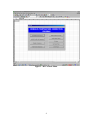
box to use the program for temperature correction of backcalculated AC moduli. The title
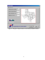
screen in Figure 1 is then displayed. If the MTCP title screen is bigger or smaller than your
computer display, you may resize the screen using the zoom box at the top toolbar of the
Excel spreadsheet. In the example shown in Figure 1, the zoom box is currently set at 100%.
Click the size you want in the zoom box or enter a number between 10 and 400 to resize the
screen.
To start using MTCP, click anywhere on the MTCP title screen to get to the main
program menu illustrated in Figure 2. From this menu, you may access the available program
functions. The available functions are described in the remainder of this user’s guide.
2
Figure 1. MTCP Title Screen.
3
Figure 2. MTCP Main Menu.
4
CHAPTER II
USING THE MODULUS TEMPERATURE
CORRECTION PROGRAM
The FWD is commonly used in Texas for pavement evaluation and design purposes.
Typically, pavement engineers make measurements at a given date so that the data reflect the
environmental conditions prevailing during the time of measurement. MTCP has been
developed to give TxDOT pavement engineers a tool for adjusting backcalculated AC moduli
to account for temperature effects. Through this program, seasonal variations in AC moduli
may be predicted for pavement evaluation and design purposes. Instructions for using MTCP
are given in this chapter.
SPECIFYING MTCP INPUT FILES
Within TxDOT, pavement engineers use MODULUS for backcalculating layer
moduli from FWD measurements. Consequently, researchers developed MTCP to use the
output from MODULUS directly. This is done by clicking on the Read MODULUS Result
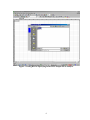
ASCII File button of the main menu given in Figure 2. Specifying the MODULUS summary
output file is the first step in using the program for temperature correction of backcalculated
AC moduli. Clicking on Read MODULUS Result ASCII File brings up the dialog box
shown in Figure 3. From this menu, the user can specify the MODULUS summary output
file to use in the analysis. Simply highlight the file by clicking on the file name in the dialog
box. Then click on the Open button at the lower right corner of the dialog box to confirm
your selection. From this menu, you may also search the different drives and subdirectories
on your computer for the particular file you want to process.
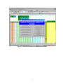
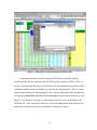
The MODULUS output file is read, and the contents of the file are imported into the
output worksheet shown in Figure 4. To view the information, click on Exit the Program to
close the main menu as illustrated in Figure 5. You may go back to this menu at any time by
pressing the Ctrl, Shift, and M keys in combination (Ctrl+Shift+M). The information
displayed in Figure 5 is the same as that given in the MODULUS summary output and
consists of the:
5
Figure 3. Dialog Box for Specifying MODULUS Output File to Analyze.
6
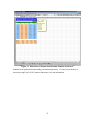
Figure 4. MODULUS Output File Imported into MTCP.
7
Figure 5. Viewing the MODULUS Summary Output File.
1. district and county where FWD measurements were taken;
2. pavement layer thicknesses;
3. allowable range of the backcalculated modulus for each layer;
4. FWD load, sensor deflections, and backcalculated layer moduli at each test
location along with the absolute error per sensor between the predicted and
measured deflections;
2. depth to bedrock estimated from the measured deflections at each station; and
3. computed means, standard deviations, and coefficients of variation for the
measured deflections, backcalculated moduli, depths to bedrock, and absolute
errors per sensor.
8
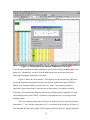
In addition, the column labeled Limit in the worksheet gives an indication of whether
any of the backcalculated moduli reached the limits set by the user during the
backcalculation. If moduli reach any limit, the program shades the cell for that particular
station red under the Limit column. Otherwise, the cell is shaded green. To the right of the
Limit column are blank cells where temperature data taken during FWD testing are entered.
Air and surface temperatures are normally measured from sensors built into the FWD and are
recorded at each test location. These measurements are written in the same data file where
the deflections are saved. For the purpose of predicting pavement temperatures using the
methods built into the program, surface temperatures taken with an infrared sensor are
required. Consequently, researchers recommend that infrared sensors be installed in
TxDOT’s FWDs to implement the computer program developed from this project. In
practice, attention must be given to maintaining the infrared sensor in good operating
condition and checking the sensor calibration to ensure the validity of the temperature
measurements.
In addition, the operator collects pavement temperatures at specific locations using a
temperature probe. For this purpose, researchers recommend that temperatures be measured
at half the depth of the surface layer if the thickness is known at the time of FWD testing, or
at a depth of 1.6 inches (4 cm) from the surface if the thickness is not known. These
recommendations are based on the findings from this study (Fernando and Liu, 2001).
Since layer thicknesses are needed to analyze the FWD deflections using MODULUS,
users may obtain this information beforehand and use it in planning the FWD testing. For
this purpose, researchers strongly suggest a Ground Penetrating Radar (GPR) survey on the
route to establish the variations in layer thicknesses from the profiles obtained. Specifically,
the GPR survey should be conducted to:
1. detect changes in pavement layer thicknesses and divide the project into analysis
segments,
2. establish the locations of FWD measurements consistent with pavement thickness
variations identified from the radar data, and
3. establish the need for cores or Dynamic Cone Penetrometer (DCP) data to
supplement the radar survey and identify locations where coring and DCP
measurements should be made.
9
Figure 6. Dialog Box for Specifying the FWD Data File.
Pavement temperatures measured during the FWD survey should be properly
recorded into the data file consistent with the FWD operator’s manual (TxDOT, 1996). In
this way, all temperature data may be read from the file and imported directly into the MTCP
spreadsheet without having to manually key in the pavement temperatures. The air, surface,
and pavement temperatures taken during the survey may be imported into the spreadsheet by
clicking on the Read FWD Test File & Get Temperatures button of the main menu given in
Figure 2. The dialog box in Figure 6 is then displayed for you to specify the name of the
FWD data file. After selecting the FWD file, click on the Open button of the dialog box to
import the temperature data into the spreadsheet as illustrated in Figure 7.
10
Figure 7. Temperature Data Imported from the FWD Data File.
PERFORMING THE TEMPERATURE CORRECTION
Before corrections to a reference temperature may be made, the pavement
temperatures you are correcting from must first be established. These pavement temperatures
are referred to herein as the base temperatures for the modulus correction and refer to the
pavement temperatures at which the FWD deflections were taken. There are two functions
available in MTCP to establish the base temperatures. One allows you to estimate the
pavement temperature at a given FWD station by interpolating between pavement
temperatures measured at two neighboring stations that bound it.
In practice, pavement temperatures will not normally be measured at each test
location. By clicking on the Interpolate Temperatures button in the main menu, you can fill
in the missing information by interpolation from the available pavement temperature
measurements. As a minimum, pavement temperatures should be measured at the beginning
11
and end of the FWD survey for a given project. The program uses a linear interpolation
based on the time of the FWD measurement. This is given in the Test Time column of the
spreadsheet illustrated in Figure 7. No extrapolation is done for locations that are outside the
range of stations where pavement temperatures were measured. Stations preceding the first
temperature measurement are assigned that pavement temperature while stations following
the last measurement are assigned the last value.
If you did not enter the pavement temperatures at the time of the FWD survey, you
may manually key in the data along the Pavement column of the spreadsheet inside the cells
corresponding to stations where pavement temperatures were taken. After manually entering
the data, you may then click on Interpolate Temperatures to fill in the rest of the cells along
the Pavement column with interpolated pavement temperatures.
Alternatively, if pavement temperatures were not measured during the survey, the
base temperatures for the correction may be established using one of three options available
within MTCP for predicting pavement temperature. All three options require the infrared
surface temperatures taken with the FWD and the average of the previous day’s minimum
and maximum air temperatures at the vicinity of the project. The first two options are the
BELLS2 and BELLS3 equations which were developed using data from Seasonal Monitoring
Program (SMP) sites located in North America. The development of these equations are
documented in a report by Lukanen, Stubstad, and Briggs (1998) and in a paper by Stubstad
et al. (1998). BELLS2 is the equation for the FWD testing protocol used in the Long-Term
Pavement Performance (LTPP) program. On the other hand, BELLS3 is intended for routine
testing and was developed from efforts made to consider the effects of shading on the
infrared surface temperatures measured on the SMP sites. The functional form of the
BELLS2 and BELLS3 equations is given by:
Td = $0 + $1 IR + [log10(d) - 1.25] [ $2 IR + $3 T(1-day) + $4 sin(hr18 - 15.5) ] +
$5 IR sin(hr18 - 13.5)
(1)
where,
Td = pavement temperature at depth, d, within the asphalt layer, °C
IR = surface temperature measured with the FWD infrared temperature gauge, °C
d
= depth at which the temperature is to be predicted, mm
12
Table 1. Coefficients of the BELLS2 and BELLS3 Equations.
Coefficient
BELLS2
BELLS3
$0
+2.780
+0.950
$1
+0.912
+0.892
$2
-0.428
-0.448
$3
+0.553
+0.621
$4
+2.630
+1.830
$5
+0.027
+0.042
R2
0.977
0.975
SEE
1.8 °C
1.9 °C
Nobs
10,304
10,304
T(1-day) =
hr18
the average of the previous day’s high and low air temperatures, °C
= time of day in the 24-hour system but calculated using an 18-hour asphalt
temperature rise and fall time as explained by Stubstad et al. (1998)
The coefficients of Eq.(1) are given in Table 1 for both the BELLS2 and BELLS3 equations.
Also shown are the R2, standard error of the estimate (SEE) and the number of observations
(Nobs) used to develop each equation. Note that the average of the previous day’s high and
low air temperatures is the only variable not collected during routine FWD testing that the
user needs to provide to predict pavement temperatures with BELLS2 or BELLS3.
Researchers recommend that pavement temperatures be predicted at half the depth of the
surface layer.
The third option available within MTCP to predict pavement temperature uses the
same variables as BELLS2 and BELLS3 but has the functional form given by Eq.(2) below:
Td = $0 + $1 (IR + 2)1.5 + log10(d) ( { $2 (IR + 2)1.5 + $3 sin2(hr18 - 15.5) +
$4 sin2(hr18 - 13.5) + $5 [T(1-day) + 6]1.5 } +
$6 sin2(hr18 - 15.5) sin2(hr18 - 13.5)
where the terms are as defined previously and the coefficients are:
13
(2)
$0 = 6.460
$1 = 0.199
$2 = -0.083
$4 = 1.874
$5 = 0.059
$6 = -6.783
$3 = -0.692
Equation (2) has an R2 of 0.931 and a standard error of the estimate of 3.1 °C with 1575
observations. It was developed using data collected from SMP sites in Texas, New Mexico,
and Oklahoma and from two flexible pavement sections located at the Texas A&M Riverside
Campus. If the pavement temperatures at these sites are predicted using the original BELLS2
and BELLS3 equations, standard errors of the estimate of 4.1 °C and 4.9 °C are obtained,
respectively (Fernando and Liu, 2001). To improve the predictive accuracy, researchers
undertook to calibrate the BELLS2 and BELLS3 equations using data that are representative
of conditions within Texas. These efforts led to the development of Eq.(2) which is referred
to as the Texas-LTPP equation.
You may access the available options for predicting pavement temperature by clicking
on the Predict Pavement Temperatures button of the main menu. This will display the
dialog box illustrated in Figure 8 where you will specify:
1. the depth, in inches, at which the temperature is to be predicted;
2. the average of the previous day’s high and low air temperatures in °F; and
3. the method for predicting pavement temperature, i.e., BELLS2, BELLS3, or the
Texas-LTPP equation given by Eq.(2).
You may select the equation to use by clicking on the down arrow in the Select Equation
field of the dialog box to display the list of available options (see Figure 9). Select the
equation by clicking on it. Note that the surface thickness from the MODULUS output file is
displayed in the dialog box for your reference when you specify the depth at which pavement
temperatures are to be predicted. It is also important that you specify the depth in inches and
the average of the previous day’s high and low air temperatures in °F as noted in the dialog
box. The program automatically converts these inputs to the corresponding metric units used
in the equations.
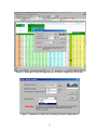
After entering the required data in Figure 8, click on the OK button of the dialog box
to proceed with the temperature prediction. The results are written into the spreadsheet
immediately to the right of the Test time column as shown in Figure 10. This column is
labeled Predicted Temperature. If you bring the pointer inside the cell for this label, a
comment box is displayed (Figure 10) which gives information on the equation selected for
predicting pavement temperatures, the depth at which the temperatures were predicted, and
14
Figure 8. Dialog Box to Specify Input Data for Pavement Temperature Prediction.
Figure 9. Equations Available for Predicting Pavement Temperatures.
15
Figure 10. Predicted Pavement Temperatures from MTCP.
the average of the previous day’s high and low air temperatures. A red triangular spot at the
upper right corner identifies cells with comment boxes. Sometimes there may be more
information than can be displayed inside the comment box. In this case, you may resize the
box by right clicking on the cell and selecting the Edit Comment function (Figure 11) to view
all of the information inside the box.
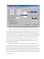
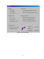
After the base temperatures are established, you can proceed with the modulus
correction by clicking on the Modulus Temperature Correction button of the main menu
illustrated in Figure 2. This will display the dialog box shown in Figure 12 which provides
the following three options for temperature correction of backcalculated AC moduli:
1. the existing TxDOT equation used in the Flexible Pavement System (FPS) and
load zoning analysis programs,
2. the Chen equation (Chen at al., 2000), and
3. Witczak’s dynamic modulus equation.
16
Figure 11. Resizing the Comment Box Using the Edit Comment Function in Excel.
17
Figure 12. Dialog Box Showing TxDOT’s Equation for Modulus Temperature
Correction.
You can select the equation to use for temperature correction by clicking on the appropriate
folder tab of the dialog box in Figure 12, where TxDOT’s equation for modulus temperature
correction is shown. This equation is based on a reference temperature of 75 °F. The
independent variables of the equation are the FWD test temperature T in °F and the
backcalculated asphalt concrete modulus ET that is read from the MODULUS summary
output file. The FWD test temperatures correspond to the base pavement temperatures
established in the previous step. As shown in Figure 12, you have two options for specifying
the base pavement temperatures. If pavement temperatures were measured during the FWD
survey, you can use the measured temperatures at specific stations and the interpolated values
at the other stations by clicking on the Use Tested Pavement Temp. option in the dialog box.
If no pavement temperatures were measured during the survey, you can use the predicted
temperatures from BELLS2, BELLS3, or the Texas-LTPP equation presented previously.
18
Figure 13. Chen Equation for Modulus Temperature Correction.
You may then perform the modulus temperature correction by clicking the Run button of the
dialog box. Alternatively, you may click the Exit button to go back to the main menu
without performing the temperature corrections.
Figure 13 shows the Chen equation. This equation was developed using FWD and
pavement temperature data taken from three test sections established as part of TxDOT’s
Mobile Load Simulator (MLS) project (Chen et al., 2000). The equation is therefore
applicable for pavements that are similar to the sections tested. Nevertheless, modulus
temperature correction factors from this equation were found to agree reasonably well with
corresponding factors from TxDOT’s equation even though the two were developed from
different studies.
The Chen equation permits the correction to be made for any user-specified reference
temperature Tr. The reference temperature (in °F) is specified in the dialog box of Figure 13.
Note that both the Chen and existing TxDOT equations do not require AC mixture properties
19
for modulus temperature correction and are thus easy to use in practice. These equations
were developed for the typical mixtures used in the state. However, there may be occasions
where the user may want to evaluate the temperature dependency for the specific asphalt mix
used in a given project. Consequently, a third option (Figure 14) was incorporated into
MTCP that is based on the prediction equation for dynamic modulus developed by Witczak
and Fonseca (1996). This option requires data on the aggregate gradation and the binder
viscosity-temperature relationship for the asphalt concrete mixture. The equation for
modulus temperature correction is given by:
log 10 E R
=
R2 = 0.93
1
1
log10 E T + A
− ( BR + 0.7425 log10 η R ) −
− ( BT + 0.7425 log10 ηT )
1+ e
1+ e
(3)
SEE = 0.12 (log scale)
where,
A
=
187
. + 0.003 p4 + 0.00004 p3/8 − 0.00018 ( p3/8 ) 2 + 0.0164 p3/ 4
(4)
BR
=
0.716 log 10 f R
(5)
BT
=
0.716 log 10 f T
(6)
ER
= AC modulus corrected for the selected reference temperature, 105 psi
ET
= backcalculated asphalt concrete modulus, 105 psi
0R
= binder viscosity corresponding to the reference temperature, 106 Poises
0T
= binder viscosity corresponding to the FWD test temperature, 106 Poises
p4
= cumulative percent retained on #4 sieve by total aggregate weight
p3/8 = cumulative percent retained on 3/8-inch sieve by total aggregate weight
p3/4 = cumulative percent retained on 3/4-inch sieve by total aggregate weight
fR
= reference loading frequency, Hz
fT
= test frequency, Hz
For the impulse loading of the FWD, the test frequency may be approximated from
the following relationship proposed by Lytton et al. (1990):
fT
=
1
2t
20
(7)
Figure 14. Dialog Box for Temperature Correction Based on Witczak’s Dynamic
Modulus Equation.
where t is the duration of the impulse load in seconds. The duration of the impulse load for
the FWD is about 30 msecs which gives a test frequency of about 16.7 Hz, the value used in
MTCP for modulus correction On the other hand, fR should correspond to the frequency of
loading used in pavement design. This typically ranges from 8 to 10 Hz for the standard 18kip single axle load traveling at typical highway speeds. The reference frequency is entered
in the fr field of the dialog box shown in Figure 14. Note that if you enter a value equal to the
FWD load frequency (16.7 Hz), no correction for the effect of load duration on the AC
modulus will be made.
The gradation information for the mix is entered in the fields labeled P4, P38, and
P34 corresponding, respectively, to p4, p3/8, and p3/4. The binder viscosity corresponding to
the reference and base pavement temperatures are determined using the ASTM D-2493
viscosity-temperature relationship given by:
21
log10 log10 η
=
A + VTS log10 T° R
(8)
where 0 is the binder viscosity, T°R is the temperature in degrees Rankine, and A and VTS are
model coefficients determined from testing. In practice, A and VTS may be determined by
conducting dynamic shear rheometer (DSR) tests at a range of temperatures on the binder
extracted from a core taken at the project site. This extraction will also provide the gradation
data needed to use the dynamic modulus equation for temperature correction.
DSR tests may be conducted at an angular frequency of 10 rad/sec and for a
temperature range of 40 to 130 °F. From the binder complex shear modulus G* and phase
angle * determined at a given temperature, the corresponding binder viscosity may be
estimated from the equation:
η
=
G * 1
10 sin δ
4 .8628
(9)
The binder viscosities determined at the different test temperatures may be used in a
regression analysis to get the A and VTS coefficients of Eq.(8). These coefficients are then
entered in the corresponding fields of the dialog box given in Figure 14.
In the absence of actual test data to determine the coefficients, researchers have
incorporated default values into MTCP to permit you to conduct an approximate analysis.
The default coefficients are based on the asphalt grade and are applicable for unmodified
binders. Table 2 shows the coefficients for AC-graded binders while Table 3 shows the
coefficients for performance-graded (PG) asphalts. The coefficients in Table 2 are based on
research conducted by Mirza (1993) and are representative of asphalts that have undergone
field aging. Those in Table 3 are from unpublished data taken from the AASHTO 2002
development work. The predicted binder viscosities from these coefficients are
representative of mix/laydown conditions.
If the binder on the project is AC-graded, you may specify the asphalt type by clicking
on the down arrow in Figure 14 to display the list of asphalt grades for which default
coefficients are available (see Figure 15). From this list, you may click on the applicable
binder type to select it. The coefficients corresponding to this binder are then displayed in
the A and VTS fields of the dialog box.
22
Table 2. Default A and VTS Coefficients for AC-Graded Asphalts1.
1
Viscosity Grade
(Original
Conditions)
Viscosity Range at
140 °F (Poises)
A
VTS
AC - 2.5
100 - 350
11.8408
-3.9974
AC - 5
350 - 700
11.4711
-3.8557
AC - 10
700 - 1400
11.0770
-3.7097
AC - 20
1400 - 2800
10.9168
-3.6469
AC - 40
2800 - 5200
10.6528
-3.5477
Representative of asphalts that have undergone field aging.
23
Table 3. Default A and VTS Coefficients for PG-Graded Asphalts1.
High
Temp.
Grade
Low Temperature Grade
-10
A
-16
VTS
A
-22
VTS
A
-28
VTS
A
-34
VTS
46
1
-40
-46
A
VTS
A
VTS
A
VTS
11.504
-3.901
10.101
-3.393
8.755
-2.905
8.310
-2.736
52
13.386
-4.570
13.305
-4.541
12.755
-4.342
11.840
-4.012
10.707
-3.602
9.496
-3.164
58
12.316
-4.172
12.248
-4.147
11.787
-3.981
11.010
-3.701
10.035
-3.350
8.976
-2.968
64
11.432
-3.842
11.375
-3.822
10.980
-3.680
10.312
-3.440
9.461
-3.134
8.524
-2.798
70
10.690
-3.566
10.641
-3.548
10.299
-3.426
9.715
-3.217
8.965
-2.948
8.129
-2.648
76
10.059
-3.331
10.015
-3.315
9.715
-3.208
9.200
-3.024
8.532
-2.785
82
9.514
-3.128
9.475
-3.114
9.209
-3.019
8.750
-2.856
8.151
-2.642
Coefficients representative of mix/laydown conditions (unpublished data from AASHTO 2002 development work).
Figure 15. Drop-Down List of AC-Graded Asphalts with Default Coefficients.
If the binder on the project is PG-graded, you simply click on the up and down arrows of
the PG fields in the dialog box until you get the number designations you want. The A and VTS
coefficients for that PG grade are then displayed. Note that coefficients are only available for
the PG grades shown in Table 3. It is also noted that the A and VTS coefficients displayed in the
dialog box always correspond to those specified for the last run made. Default values for these
coefficients may have been used, or alternatively, coefficients from laboratory test data may
have been entered in the A and VTS fields of the dialog box shown in Figure 15. Thus, these
fields will not necessarily display coefficients that correspond to the current AC and/or PG
grades displayed in the dialog box.
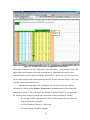
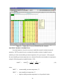
The results from the temperature corrections are written into the worksheet along the
column labeled Corrected Modulus. As shown in Figure 16, the column label has a comment
box which gives information about the method used to perform the temperature correction.
Specifically, the comment box identifies the method, as well as the reference and base pavement
temperatures used for the corrections. In addition, if the dynamic modulus equation is selected,
the A and VTS coefficients, reference loading frequency, and aggregate gradation are displayed
in the comment box.
25
Figure 16. Temperature Corrected Moduli from the Analysis.
MONTHLY MODULUS PREDICTION
In certain instances, it may be necessary to model the seasonal variation in material
properties. MTCP permits the user to estimate the monthly variation in asphalt concrete
modulus given the mean monthly pavement temperatures for a given project. In the program,
the mean monthly pavement temperatures are estimated from the mean monthly air temperatures
using the following equation (Asphalt Institute, 1982):
MMPT
=
1
34
MMAT 1 +
+ 6
−
( z + 4) ( z + 4)
where,
MMPT =
mean monthly pavement temperature, °F
MMAT = mean monthly air temperature, °F
z
= depth at which pavement temperature is to be predicted, inches
26
(10)
As an aid in using this feature, a database of mean monthly air temperatures has been
compiled that covers all counties in the state. This database is built in to MTCP and is used to
estimate the mean monthly pavement temperatures. The reference modulus corresponding to the
reference temperature is then adjusted to the predicted mean monthly pavement temperatures.
By default, the reference modulus is taken as the average of the corrected moduli for the
different stations. Thus, in performing the temperature correction for the backcalculated asphalt
concrete moduli, the user may specify a reference temperature that he or she considers
representative of the year-round pavement temperatures at the project surveyed. In this instance,
the corrected moduli will correspond to average yearly conditions at the site. To evaluate
monthly variations, the average of the corrected moduli is adjusted to the predicted mean
monthly pavement temperatures in MTCP.
Alternatively, the user may correct the backcalculated moduli to a reference temperature
that he or she considers to be representative of the pavement temperatures at the time of the
FWD survey. In this instance, the program will predict how the reference modulus,
corresponding to conditions at the date of testing, varies with the predicted monthly changes in
pavement temperatures at the site surveyed.
While the program uses the average of the corrected moduli as the default reference for
evaluating monthly variations, the user may specify an alternative reference value for the
analysis. This option is described later. At this point, a few guidelines about the selection of the
reference modulus are in order.
The user should examine the variation in the corrected moduli for the different stations
tested. If the coefficient of variation exceeds 15 percent, the user should ask whether the
variability suggests possible differences in pavement materials and layer thicknesses along the
route surveyed. He or she should check the measured deflections, backcalculated moduli,
predicted depths to bedrock, the average absolute errors per sensor, and whether any of the
prescribed limits were reached in the backcalculation. Depending on the results, there may be a
need to subsection the FWD data to create homogeneous segments for the MODULUS
backcalculation. For this purpose, the MODULUS program may be used to delineate segments
of a specified minimum length based on the cumulative difference method. Michalak and
Scullion (1995) describe how this option is used in MODULUS.
27
The user may have to collect additional information on the route to better characterize
the pavements for the segments identified. The MODULUS and temperature correction
programs are then run on each segment. Results from these runs should be reviewed to establish
the need for further analyses.
To predict how the asphalt concrete modulus at the site will vary with temperature
changes over the year, click on the Monthly Modulus Prediction button of the MTCP main
menu. The dialog box shown in Figure 17 is then displayed. This dialog box shows the
averages of the daily minimum and daily maximum air temperatures for each month, as
determined from the weather station in the county where the project surveyed is located. The
average monthly air temperatures are also shown as well as the name, elevation, and location of
the weather station. The county ID displayed in the dialog box is read directly from the FWD
data file. If for some reason, the county ID in the file is wrong, you may simply type the correct
ID in the dialog box or use the up and down buttons beside the County ID field to scroll through
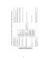
the weather data for the different counties in Texas. A list of the counties is given in Figure 18
for your reference.
After establishing the county ID for the project, click on the folder tab labeled Input in
the dialog box. The screen shown in Figure 19 is then displayed where you may specify:
1.
the depth at which the mean monthly pavement temperatures will be predicted,
2.
the reference temperature, and
3.
the reference modulus.
For consistency, the depth and the reference temperature are the same as that specified in the
correction of the backcalculated asphalt concrete moduli. For your reference, the thickness of
the surface layer is also provided. The reference modulus shown is the average of the corrected
moduli, as explained earlier. You may change any of these default values, but you need to make
sure that the values you input are consistent with each other.
When you are through specifying the input parameters for this dialog box, click on the
Next button to continue. The screen shown in Figure 20 is then displayed. You will notice that
the mean monthly pavement temperatures are calculated and written into a new worksheet
labeled Month. In addition, the average monthly air temperatures and the reference modulus are
reported in the worksheet. There is also a dialog box where you can specify the equation you
want to use for correcting the reference modulus to the predicted mean monthly pavement
temperatures. The two choices available are the dynamic modulus and Chen equations. To
28
Figure 17. Dialog Box of Monthly Air Temperatures for Specified County.
29
Figure 18. List of Texas Counties by District (TxDOT, 1998).
30
Figure 19. Dialog Box of Input Parameters for the Monthly Modulus Prediction.
31
Figure 20. Dialog Box to Specify Equation for Monthly Modulus Prediction.
specify which equation to use, simply click on its folder tab. Note that if you used the dynamic
modulus equation to correct the backcalculated AC moduli, the A and VTS coefficients you
previously specified are displayed in the dialog box as well as the reference loading frequency
and the gradation of the asphalt mix. While you may change these variables in the dialog box, it
is important that the values you enter are consistent with the method employed to correct the
backcalculated AC moduli. In most applications, it is likely that you would only have to click
on the Run button of the dialog box to perform the monthly modulus predictions based on the
dynamic modulus equation without having to change any of the data shown. To select the Chen
equation, click on its folder tab and then on the Run button of the dialog box to perform the
analysis.
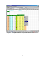
Figure 21 illustrates the output from the evaluation of monthly modulus variation. The
predicted modulus for each month is written in the last column of the worksheet. The label for
this column also has a comment box that reports the parameters used in correcting the reference
32
Figure 21. Illustration of Output from Monthly Modulus Prediction.
modulus to the predicted mean monthly pavement temperatures. You may resize the box as
necessary using Excel’s Edit Comment function to view the information.
33
CHAPTER III
MTCP OUTPUT
GETTING OUTPUT OF ANALYSIS RESULTS
As presented in Chapter II, there are two worksheets created by MTCP which have the
input data used in the analyses as well as the results. The output worksheet contains the
summary output from the MODULUS backcalculation; the measured air, surface, and pavement
temperatures from the FWD survey; the predicted pavement temperatures; and the corrected
asphalt concrete moduli. The other worksheet, labeled Month, has the monthly average air
temperatures, the predicted mean monthly pavement temperatures, and the predicted monthly
variation in asphalt concrete modulus for the material tested. You may print each of these
worksheets using the Print function available in Excel. You may also produce charts of the
results by clicking the Plot Output button of the MTCP main menu. This will bring up the chart
selection menu illustrated in Figure 22.
Table 4 describes the chart options available from the menu. The default worksheet
names shown in the table are reserved for program use. You may not use any of these names to
label worksheets that you manually create in the Excel spreadsheet. Note that the charts which
may be produced depend on the main menu functions that have already been executed. For
example, neither the FWD nor MODULUS summary output data may be plotted until the data
files have been read by MTCP. Similarly, the corrected asphalt concrete moduli and the
predicted monthly variations in the AC modulus cannot be plotted until the temperature
corrections and the monthly modulus predictions have been made.
To select a chart from the menu, simply click on its checkbox. You may select all charts
at once by clicking on the Select All button of the menu. If you wish to undo any selection, click
again on the chart’s checkbox. To undo all selections at once, click the Clear button of the
menu. The button labeled Reverse Select will undo previous selections you have made while at
the same time checking the boxes of charts not previously selected. Thus, Reverse Select has
the same effect as Clear if all of the available charts were previously selected.
35
Figure 22. MTCP Plot Menu.
36
Table 4. Available Charts in MTCP.
Chart Group
Basic Plot
Modulus
Result Plot
Monthly
Analysis Plot
Temperature
Plot
Temperature
with Modulus
Chart Label
Description
Default Worksheet
Name
Load vs Station
Plot of measured FWD load for stations tested
Load
R1 ~ R7
FWD sensor deflections plotted for each station
Deflec-1
R1 & R7
Plot of FWD sensor 1 and sensor 7 deflections by
station
Deflec-2
Modulus vs Station
Plot of backcalculated layer moduli for each
station
Err/Sens vs Station
Plot of the average absolute errors per sensor for
the different stations tested
Err
Depth to Bedrock
vs Station
Plot of the depths to bedrock predicted from the
sensor displacements measured at the different
stations
DB
Monthly Ave. Air
& Pave. Temp.
Mean monthly average air temperatures and
predicted mean monthly pavement temperatures at
the project surveyed
Month-1
Monthly Modulus
vs Month
Bar chart of predicted monthly variations in AC
modulus
Month-2
Air, Surface, &
Pavement Temp. vs
Station
Plot of air, surface, and pavement temperatures by
station
Temp-1
Tested &
Calculated
Pavement
Temperature vs
Station
Plot of measured vs predicted pavement
temperatures by station
Temp-2
Pavement Temp. vs
Modulus (before
correction)
Plot of backcalculated AC modulus versus
pavement temperature
Mod-Temp-1
Corrected & Uncorrected Modulus
(station)
Plot of corrected and backcalculated AC moduli
by station
Mod-Temp-3
Corrected & Uncorrected Modulus
(temperature)
Plot of corrected and backcalculated AC moduli
versus pavement temperature
Mod-Temp-4
37
Modu
Once you have made your selections, click on the PLOT button. Each chart selected gets
drawn on a separate worksheet. Table 4 identifies the worksheets assigned to the different
charts. To view the charts, first leave the plot menu by clicking on its Exit button. This brings
you back to the program main menu. From here, click on Exit the Program. You may then
view a particular chart by clicking on its worksheet tab which you may identify from Table 4.
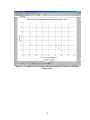
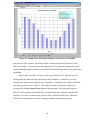
Figures 23 and 24 illustrate two of the charts that you may produce from MTCP. To print a
given chart, simply bring that chart into view by clicking on its worksheet tab. Then use Excel’s
Print function to get a hardcopy.
The plots that you generate in the spreadsheet are automatically updated as data get
changed. This situation occurs, for example, when you do another analysis using a temperature
correction equation that is different from that used to generate the charts initially. In this
instance, you do not have to rerun the plot function to get the same charts using the new analysis
results. However, you have the option to generate additional charts that were not selected in the
previous analysis.
You may also rename the chart worksheets in Excel. To use a name different from the
default value given in Table 4, simply double click the tab of the worksheet you wish to rename.
Then type in the label that you want that worksheet to have and press the Enter key.
Alternatively, you may right click on the worksheet tab and select the Rename function in Excel
to re-label the selected worksheet.
SAVING THE ANALYSIS RESULTS
Once you finish with your analysis, you may save your results by using Excel’s Save or
Save As function. To do this, you must first exit the MTCP main menu by clicking on Exit the
Program. Then you may click on the Save icon in the top toolbar to save your results using the
default file name assigned by the program. The Excel spreadsheet, with all the accompanying
data and charts, is saved in a file with the same name as the MODULUS summary output file
but with the extension XLS.
If you do not wish to use the default file name, you may save the spreadsheet using
the Save As function in Excel’s File menu. Click on File at the top of the spreadsheet, then
on Save As. A dialog box will then be displayed where you can specify the name of the file
where the results will be saved. In addition, you may specify the drive and subdirectory
38
Figure 23. Example Plot of Corrected and Backcalculated AC Moduli vs Pavement
Temperature.
39
Figure 24. Example Plot of Predicted Monthly Variations in AC Modulus.
where this file will be written. By default, the file is written in the same subdirectory where
MTCP was loaded. You may open the spreadsheet in Excel at a later time should you wish to
conduct additional analyses with the same MODULUS and FWD input files used to generate the
spreadsheet.
After saving your results, you may exit Excel by clicking on File, then on Exit or by
clicking on the X button at the top right corner of the spreadsheet. Alternatively, you may
conduct a new analysis with a different set of input data. To perform a new analysis, reload the
main menu by pressing Ctrl+Shift+M. Then clear the results of the previous analysis by
clicking on the Clear Program Sheets button of the main menu. The dialog box shown in
Figure 25 will be displayed to confirm that you wish to delete the worksheets created by the
program. If you have saved the results, you may click on Yes in the dialog box. Otherwise,
click No for an opportunity to save the existing spreadsheet as described previously.
40
Figure 25. Dialog Box to Delete Program Worksheets Prior to a New Analysis.
After the existing program worksheets have been deleted, the main menu is again
displayed. From here, the user may read another MODULUS output file and conduct a new
analysis as described in this user’s guide. It is noted that the Clear Program Sheets function
will only delete the worksheets created by the program (identified in the dialog box shown in
Figure 25). Worksheets that were manually created by the user during the previous analysis
are not deleted.
41
REFERENCES
Asphalt Institute. Research and Development of the Asphalt Institute’s Thickness Design
Manual (MS-1) Ninth Edition. Research Report No. 82-2, Asphalt Institute, Ky., 1982.
Chen, D., J. Bilyeu, H. Lin, and M. Murphy. Temperature Correction on FWD Measurements.
Paper presented at the 79th Annual Meeting of the Transportation Research Board (accepted for
publication), Washington, D. C., 2000.
Fernando, E. G., and W. Liu. Development of a Procedure for Temperature Correction of
Backcalculated AC Modulus. Research Report 1863-2, Texas Transportation Institute, Texas
A&M University, College Station, Tex., 2001.
Fernando, E. G., and W. Liu. Program for Load-Zoning Analysis (PLZA): User’s Guide.
Research Report 2123-1, Texas Transportation Institute, Texas A&M University, College
Station, Tex., 1999.
Fernando, E. G. PALS 2.0 User’s Guide. Research Report 3923-1, Texas Transportation
Institute, Texas A&M University, College Station, Tex., 1997.
Jooste, F. J., and E. G. Fernando. Development of a Procedure for the Structural Evaluation of
Superheavy Load Routes. Research Report 1335-3F, Texas Transportation Institute, Texas
A&M University, College Station, Tex., 1995.
Lukanen, E. O., R. N. Stubstad, and R. C. Briggs. Temperature Predictions and Adjustment
Factors for Asphalt Pavements. Research Report FHWA-RD-98-085, Federal Highway
Administration, McLean, Va., 1998.
43
Lytton, R. L., F. P. Germann, Y. J. Chou, and S. M. Stoffels. Determining Asphaltic Concrete
Pavement Structural Properties by Nondestructive Testing. National Cooperative Highway
Research Program Report 327, Transportation Research Board, Washington, D. C., 1990.
Michalak, C. H., and T. Scullion. MODULUS 5.0: User’s Manual. Research Report 1987-1,
Texas Transportation Institute, Texas A&M University, College Station, Tex., 1995.
Mirza, M. W. Development of a Global Aging System for Short and Long Term Aging of
Asphalt Cements. Ph.D. Dissertation, University of Maryland, College Park, Md., 1993.
Stubstad, R. N., E. O. Lukanen, C. A. Richter, and S. Baltzer. Calculation of AC Layer
Temperatures From FWD Field Data. Proceedings, Fifth International Conference on the
Bearing Capacity of Roads and Airfields, Vol. 2, Trondheim, Norway, 1998, pp. 919 – 928.
Texas Department of Transportation. Pavement Management Information System Rater’s
Manual for Fiscal Year 1999. Texas Department of Transportation, Austin, Tex., 1998.
Texas Department of Transportation. Falling Weight Deflectometer Operator’s Manual. Texas
Department of Transportation, Austin, Tex., 1996.
Witczak, M. W. and O. A. Fonseca. Revised Predictive Model for Dynamic (Complex) Modulus
of Asphalt Mixtures. Transportation Research Record 1540, Transportation Research Board,
Washington, D. C., 1996, pp. 15 – 23.
44
45
46