1
Title:
SG52 MICROSCOPES
Department: STEP
Document No: OP/EQP/LS/46
Revision A.1
Standard Operating Procedure
SG52 MICROSCOPES
Page 1 of 31
Title:
SG52 Microscopes
Department: STEP
Document No: OP/EQP/LS/46
Revision A.1
Table of Contents
1
THE BASICS ................................................................................................................................................................... 3
1.1
GROUND RULES .......................................................................................................................................................... 3
1.2
MT20 (BURNER) OPERATION ...................................................................................................................................... 3
1.3
ANATOMY OF A MICROSCOPE ..................................................................................................................................... 4
1.3.1
Transmission Light Source (Halogen) ............................................................................................................... 5
1.3.2
Reflection Light Source (Arc Burner) ................................................................................................................ 5
1.3.3
Transmission filters / diffusers ........................................................................................................................... 5
1.3.4
Field Stop ........................................................................................................................................................... 5
1.3.5
Condenser Assembly (and Aperture Stop) ......................................................................................................... 5
1.3.6
Stage .................................................................................................................................................................. 5
1.3.7
Objective Lens Turret ........................................................................................................................................ 5
1.3.8
Filter Wheel ....................................................................................................................................................... 5
1.3.9
Eyepieces ........................................................................................................................................................... 5
1.3.10
Sideports ............................................................................................................................................................ 5
1.4
BASIC SETUP .............................................................................................................................................................. 6
1.4.1
Power up/down procedure ................................................................................................................................. 6
1.4.2
Köhler Illumination (Brightfield) ....................................................................................................................... 6
1.4.3
Eyepieces ........................................................................................................................................................... 7
1.4.4
Darkfield Illumination ....................................................................................................................................... 8
1.4.5
Phase Contrast ................................................................................................................................................... 9
1.4.6
Differential Interference Contrast ................................................................................................................... 11
1.5
MICROSCOPE CARE ................................................................................................................................................... 13
1.6
SOME HANDY TERMS AND TIPS... .............................................................................................................................. 14
1.6.1
Common Nomenclature ................................................................................................................................... 14
1.6.2
Aberrations ...................................................................................................................................................... 15
1.7
OBJECTIVES .............................................................................................................................................................. 17
1.7.1
Using an immersion objective .......................................................................................................................... 18
1.8
FILTERS .................................................................................................................................................................... 18
1.9
SG52 MICROSCOPES................................................................................................................................................. 20
2
BASIC OLYMPUS SOFTWARE ................................................................................................................................ 21
2.1
BASIC TRANSMISSION IMAGING ............................................................................................................................... 21
2.2
TIME LAPSE EXPERIMENTS ....................................................................................................................................... 22
2.3
REFLECTION (FLUORESCENT) IMAGING .................................................................................................................... 23
2.4
WORKING WITH REGIONS OF INTEREST .................................................................................................................... 26
2.4.1
Defining the Region of Interest ........................................................................................................................ 26
2.4.2
Making a measurement of a ROI ..................................................................................................................... 28
2.4.3
Background Subtraction .................................................................................................................................. 28
The electronic version of this document is the latest version. It is the responsibility of the individual to ensure that any paper
material is the current version. Printed material is uncontrolled documentation.
Last Revised 13th October 2014
Page 2 of 31
Title:
SG52 Microscopes
Department: STEP
Document No: OP/EQP/LS/46
Revision A.1
1 THE BASICS
1.1
Ground rules
1.2
MT20 (burner) operation
1
2
If in doubt about any of this, consult one of the people on listed on the front page. We’d be delighted to
help.
DON’T change any components on the microscopes without consulting the relevant staff.
DON’T attempt to clean any optics unless you have been trained.
Please use both the log books and booking system.
http://ncsrbooking.dcu.ie/booking/
Be considerate to other users.
There’s plenty of information here...
http://www.olympusmicro.com/primer/techniques
The burners for the MT20 cost a lot of money. Not following the rules will be punishable by having to buy
a new burner.
DO NOT forget to switch the burner off at the end of the day.
1
DO NOT run the burner for short times . Plan your experiment. If somebody is using the microscope
after you, contact them and see if they want it left on.
2
If the burner has been switched off, allow 30 mins to cool before switching back on .
Please log any burner related errors or messages.
Please ensure theMT20 exhaust is not obstructed (e.g. curtains/paper/walls) to avoid overheating.
The issue here is the extreme change in temperatures. This shortens burner lifetime.
Again, we are avoiding thermal cycling.
The electronic version of this document is the latest version. It is the responsibility of the individual to ensure that any paper
material is the current version. Printed material is uncontrolled documentation.
Last Revised 13th October 2014
Page 3 of 31
Title:
SG52 MICROSCOPES
Department: STEP
Document No: OP/EQP/LS/46
1.3
Revision A.1
Anatomy of a microscope
Figure 1-1
A Microscope
The microscopes in SG52 are inverted microscopes so these will be the kind discussed here. Figure 1-1 shows
a schematic of an inverted microscope.
1. Transmission Light Source
2. Reflection Light Source
3. Transmission filters/diffusers
4. Field Stop
5. Condenser Assembly (and Aperture Stop)
6. Stage
7. Objective Lens Turret
8. Filter Wheel
9. Eyepiece
10. Sideport
Page 4 of 31
Title:
SG52 Microscopes
Department: STEP
Document No: OP/EQP/LS/46
Revision A.1
1.3.1 Transmission Light Source (Halogen)
All the microscopes have 2 lamps: One for transmission, one for reflection.
Transmission mode allows modes such as Phase Contrast or DIC. Usually, it is white light from a tungsten
filament. You will need to buy a filter to insert in the beam path if you want to use a particular wavelength. Using
a filter cube does not make any sense here, so be sure to set the filter wheel so no filter is present.
1.3.2 Reflection Light Source (Arc Burner)
In reflection mode, the light passes through the objective, reflects off the sample and goes back through the
objective. This mode is best used for fluorescence imaging as the filter cubes only work properly in this mode.
DIC and Phase Contrast are not possible in this mode.
The lamps for reflection vary with the microscopes. They will either be a high power mercury short-arc lamp or
xenon arc lamp. The arc lamps are housed in units called the MT20. These provide very high power illumination
required by the Andor and Hamamatsu cameras for high speed imaging.
1.3.3 Transmission filters / diffusers
A diffuser is in place in the lamp housing to prevent direct imaging of the tungsten filament at low magnifications.
The diffuser may be moved out of the light path when using high magnifications. There is the option of using
other optical filters for fluorescence techniques which also may be moved in and out of the light path as required.
1.3.4 Field Stop
This is the first iris diaphragm, useful when setting up Kölher illumination.
1.3.5 Condenser Assembly (and Aperture Stop)
The condenser assembly creates a concentrated cone of light to illuminate the sample. It contains a couple of
lenses to do this and a number of components which can be switched in at will, either phase rings or DIC prisms
(or nothing when brightfield illumination is required). The condenser also contains an iris diaphragm, known as
the aperture stop.
1.3.6 Stage
Put your samples on the stage.
1.3.7 Objective Lens Turret
This is a rotating turret which will contain a number of objective lenses.
1.3.8 Filter Wheel
The microscopes have slots available for 6 filters. Most of the filters are used in reflection mode. In transmission
mode, there is a blank position with no filter for brightfield imaging (section 1.4.1) or a DIC prism (section 1.4.5)
which should be used.
1.3.9 Eyepieces
If the image is not directed to one of the cameras, you should see some sort of image here.
1.3.10 Sideports
These are used to attach a number of cameras; you typically have to select a mirror position to direct the light to
and from the sideports.
The electronic version of this document is the latest version. It is the responsibility of the individual to ensure that any paper
material is the current version. Printed material is uncontrolled documentation.
Last Revised 13th October 2014
Page 5 of 31
Title:
SG52 MICROSCOPES
Department: STEP
Document No: OP/EQP/LS/46
1.4
Revision A.1
Basic Setup
1.4.1 Power up/down procedure
Note: Manual microscope
1. Power up procedure:
Turn on microscope – all parts of microscope are on a single power strip. Switching on the socket will
turn the lamp, cameras etc.
If measuring fluorescence, turn on MT20 using switch on box at far left.
Note: DO NOT turn on the source if you do not intend to use it (i.e. for brightfield measurements)!
Turn on Computer
Start Cell F software
2. Power down procedure:
Remove sample from stage.
Turn off burner in software.
Return to 4X objective.
Wait for burner to cool.
Close down Cell F software.
Shut down computer.
Turn off MT20.
Note: MT20 MUST be left switched on for the fans to cool the lamp for at least 10 min after being
switched off. The Burner should not be switched back on for 30 mins. Frequently switching a burner on
and off reduces its lifetime. If the burner will definitely be used again (by you or someone else) within a few
hours, burner should be left on and the next person to use it should be notified.
1.4.2
Köhler Illumination (Brightfield)
Kölher illumination only has to be setup for transmission imaging!
There is an optimum illumination setup to achieve the best results. This makes sure you don’t image the actual
light source and gain the most even illumination with a minimum of unwanted scattering. This should be used for
both reflection and transmission. You don’t have to worry about it so much in reflection, so we’ll only be covering
the transmission setup.
The condenser provides even illumination to the sample. The goal is to set up an image of the field stop in the
same focal plane as your sample.
1. The condenser wheel should be set to the brightfield position, and you should be getting some light onto the
sample.
2. Focus your sample roughly.
Page 6 of 31
Title:
SG52 Microscopes
Department: STEP
Document No: OP/EQP/LS/46
Revision A.1
3
3. If you are using 4x objectives, use the diffuser .
4
4. Close the Field Stop down all the way.
Figure 1-2 Foccussed image of Field Stop
5. Adjust the height of the condenser until you can see a clear image of the Field Stop through the eyepieces like
in Fig.1.2.
Note: This might not be possible at high magnifications, so use a lower mag to get the condenser and
Aperture Stop image into position.
6. Open up the field stop do you can just see the edges in the field of view. Centre the image of the Field Stop
using the two screws at the front of the condenser.
7. Open up the Field Stop just until you can no longer see the edges of it in the field of view. (If you open it all the
way you’ll be getting a lot of scattered light, this won’t give you a great image)
5
8. Adjust the Aperture Stop for best effect.
For oil immersion, the Aperture Stop should be open all the way.
In air, closing the Aperture Stop improves contrast, but also highlights diffraction artefacts. So it’s best to
try and find the middle ground.
1.4.3
Eyepieces
The eyepieces provide a final magnification and an image plane on which it is easy for the eye to focus. They
6
can be used with and without glasses. The best viewing position is a cm or two away . What you should be
7
seeing if everything is correctly adjusted, is a single round image that is comfortable to look at .
3
The diffuser is frosted glass on top of the microscope next to the light source which can be easily swung in and out of the
beam.
4
That is the variable aperture at the top of the microscope (Number 3)
5
That is the one in the condenser
6
Please use both eyepieces, it really is less straining over long periods, and we shelled out for stereo microscopes so you
may as well use them.
The electronic version of this document is the latest version. It is the responsibility of the individual to ensure that any paper
material is the current version. Printed material is uncontrolled documentation.
Last Revised 13th October 2014
Page 7 of 31
Title:
SG52 Microscopes
Department: STEP
Document No: OP/EQP/LS/46
Revision A.1
Eyepiece separation
The distance between eyepieces is adjustable as well; simply move the eyepieces together or apart to suit the
interpupillary distance.
Again, it’s a good idea to remember the position for your own ease and comfort.
Then you can just sit down at any microscope and adjust to suit in seconds.
Individual eyepiece focus
On every microscope, one of the eyepieces will have an adjustable focus to account for differences between
eyes. The adjustable eyepiece will have a graduated scale printed on it.
The best procedure for this is to:
1. Focus your sample with the fixed eyepiece (using one eye)
2. Rotate the other eyepiece whilst looking through it, thus adjusting it to produce the best image.
This should only need to be done once, as the main microscope focus should suffice for all subsequent samples
and objectives.
Power up It’s a good idea to remember this position from the scale so you can set up on any microscope with
minimum hassle afterwards.
1.4.4 Darkfield Illumination
Note: Colour Microscope Only
Darkfield imaging utilises scattered light as opposed to reflected/absorbed light (see 1.4.1). The advantages of
dark field imaging are that objects below the diffraction limit can be imaged in fluorescence or sideband
excitation and live and unstained samples may be examined. However, high intensity illumination must be used
and setup can be tricky. For this reason unstained samples or samples using unquenchable fluorophores are
best used.
Darkfield imaging requires a special condenser assembly. The condenser body (IX2-DICD) also contains a
polariser and prism for use with DIC (see section 1.4.5). The dark field condenser lens (IX2-TLW) can be used
8
with or without an immersion fluid (which is WATER ). The working distance is 3.7mm which is ideal for inverted
samples. Because of the large working distance, the surface tension of water is not high enough to maintain a
suitable droplet. So an o-ring or petri dish to contain the water is a good idea (for an inverted sample, the 1mm
thickness of the slide may be enough to preclude such a measure).
7
Also, if you have conjunctivitis it is good practice to simply wear glasses (safety or corrective) to reduce the risk of
passing it on.
8
Don’t forget to check your objective lens to see if it requires oil, water or nothing…
The electronic version of this document is the latest version. It is the responsibility of the individual to ensure that any paper
material is the current version. Printed material is uncontrolled documentation.
Last Revised 13th October 2014
Page 8 of 31
Title:
SG52 Microscopes
Department: STEP
Document No: OP/EQP/LS/46
Revision A.1
Figure 1-3 the same sample imaged in Brightfield (Left) and Darkfield (Right) illumination
1. Engage the darkfield condenser by tilting back the support column. Loosen the grub screw on the side of the
support column. Swing the condenser into place. Tighten the grub screw whilst rocking the condenser slightly
side to side to properly locate the condenser.
2. Focus the sample and obtain Köhler Illumination. This can be tricky as the aperture won’t be imaged clearly.
3. Temporarily remove an eyepiece and observe the darkfield light disc and stop.
4. Use the stage centring screws to centre the DF condenser so that the bright disk is completely covered by the
central stop.
5. Replace the eyepiece.
6. Adjust the barrel of the DF condenser until a decent dark field image is obtained. The condenser lens will be
quite close to the sample. So be careful you don’t cause a crash.
7. Fiddle around hits the settings a bit to try and get a nice image.
1.4.5 Phase Contrast
Note: Colour Microscope Only
When you setup the optics to use phase contrast, the technique is the same as for brightfield imaging
(mentioned above). However, phase contrast is set up only on the manual microscope, so you won’t have
software control over the optics.
Phase Contrast is a technique primarily used to image transparent objects on a transparent substrate. It
accentuates differences in thickness by using the phenomenon of phase shifts which occur due to the differing
path lengths of the light through the sample. The greater the optical path length, the greater the phase shift
which results in darker portions of the image.
The electronic version of this document is the latest version. It is the responsibility of the individual to ensure that any paper
material is the current version. Printed material is uncontrolled documentation.
Last Revised 13th October 2014
Page 9 of 31
Title:
SG52 Microscopes
Department: STEP
Document No: OP/EQP/LS/46
Revision A.1
Phase contrast requires special optical elements to work. In the condenser assembly there are a number of
phase slits which provide a ring of light. In a phase contrast enabled objective, there is a phase plate as shown
9
in Figure 1.4 .
Figure 1-4: A phase plate inside an objective lens
Setting Up Phase Contrast Imaging
1. Set up Kohler illumination (see section 1.4.1)
2. Ensure you are using the right phase annulus that corresponds to the objective. There are a bunch of
these in the condenser, simply rotate by hand until you have the one you want.
That’s it! You can tell if things are going right when edge features of your sample glow brighter than the
background.
Optimising Phase Contrast Imaging
You can cause problems for yourself if you try this without knowing what you are doing. Contact your local
friendly technician for assistance.
1. Set up Kohler illumination (see section 1.4.1)
2. Engage the correct phase annulus for the objective. Remove an eyepiece and look into the microscope.
The phase telescope is in the ocular tube just below the eyepieces, rotate the barrel from the 0 position
to the CT position. You should see a bright ring (the result of the phase slit in the condenser assembly)
superimposed on a dark ring (the result of the phase ring in the objective).
3. Bring the bright ring and dark ring into focus using the focus wheel on the ocular barrel (NOT the
condenser or stage focus).
9
It is possible to use these objectives in brightfield, simply select the BF position in the condenser assembly.
The electronic version of this document is the latest version. It is the responsibility of the individual to ensure that any paper
material is the current version. Printed material is uncontrolled documentation.
Last Revised 13th October 2014
Page 10 of 31
Title:
SG52 Microscopes
Department: STEP
Document No: OP/EQP/LS/46
Revision A.1
4. If necessary use the centering screws on the condenser assembly to centre the phase contrast ring, so
that the bright ring overlaps the dark ring symmetrically.
5. Rotate the barrel back to the normal position. (That would be the "0" position.)
6. Widen the field iris diaphragm opening until the diaphragm image circumscribes the field of view.
7. Don’t forget to put the barrel back to 0 position.
1.4.6
Adjusting the aperture stop when you are set up may improve results.
Double check you are using the correct annulus for your objective.
Differential Interference Contrast
DIC can be considered complimentary to Phase Contrast in that it also utilizes phase information to produce an
image. The most notable difference between Phase Contrast and DIC is that DIC highlights large gradients of
refractive index.
As far as which is the best to use.....? DIC has a number of traits which are superior to Phase Contrast, but you’ll
just have to try both!
Photobleaching Avoision Bonus
Because DIC (and phase contrast) use relatively low levels of light compared to brightfield and the burners, DIC
can also be used to reduce the effects of photobleaching.
Simply locate the region of interest using DIC and when everything is set up, switch to fluorescent imaging. Note
that both the light sources need to be on and blanked off accordingly.
Setting Up DIC Imaging
DIC is set up using the standard brightfield condenser. It can also be done using the dark field condenser, but
the dark field aperture must be removed and replaced with a polariser (we’re not going to cover this here
though).
We need to employ the configuration shown in Fig. 1.5 with two polariser/prism pairs both above and below the
sample. The Lower Prism and Upper Polariser are shown in Fig.1.6.
The electronic version of this document is the latest version. It is the responsibility of the individual to ensure that any paper
material is the current version. Printed material is uncontrolled documentation.
Last Revised 13th October 2014
Page 11 of 31
Title:
SG52 Microscopes
Department: STEP
Document No: OP/EQP/LS/46
Revision A.1
Figure 1-5: DIC prism / polariser locations
Figure 1-6: The lower DIC Prism and Upper Polariser
The electronic version of this document is the latest version. It is the responsibility of the individual to ensure that any paper
material is the current version. Printed material is uncontrolled documentation.
Last Revised 13th October 2014
Page 12 of 31
Title:
SG52 Microscopes
Department: STEP
Document No: OP/EQP/LS/46
Revision A.1
1. Set up Köhler illumination in brightfield. (See section 1.4.1)
2. Place the polariser on the condenser.
3. Engage the Polariser in the filter wheel below the objectives.
4. Remove an eyepiece and rotate the polariser until the pattern visible in Fig.1.7 is visible.
5. Slide the DIC prism under the objective.
6. Engage the appropriate DIC prism in the condenser.
10
7. By moving the slider of the prism, we can adjust the level of wave retardation .
Figure 1-7: Desired Polarisation Pattern for DIC
1.5
Microscope care
Know your working distances.
It’s very easy to damage the objectives. Some of them are sprung to absorb collisions, but relying on this should
really be a last resort. Knowing the working distance will allow you to get into focus quickly and easily. Inscribing
a small "x" onto the cover slip or specimen with a diamond scribe or fine point marker may help you identify the
focal plane. Don’t forget that the high magnification lenses require your sample to be "upside-down". In this case,
mounting a coverslip is a must.
Know how to clean an objective.
We can teach you how to clean optics (but better if we do it for you), but the best practice is to avoid them
getting dirty in the first place.
Do not touch any optics.
Do not blow on optics to clean them.
10
You will know if you done this correctly when you see all the pretty colours!
The electronic version of this document is the latest version. It is the responsibility of the individual to ensure that any paper
material is the current version. Printed material is uncontrolled documentation.
Last Revised 13th October 2014
Page 13 of 31
Title:
SG52 Microscopes
Department: STEP
Document No: OP/EQP/LS/46
Revision A.1
Clean dry air from the wall is best. Cans of compressed air can mark surfaces if used incorrectly.
The filters cannot be cleaned, do not attempt it.
In some cases the filter will operate better with that fingerprint than the cleaning process that removes some of
11
the layers .
1.6
1.6.1
Some handy terms and tips...
Common Nomenclature
Numerical Aperture
This is a measurement of the "light-gathering" power of an element or system. It is directly linked to the resolving
power of the system. The higher the N.A. the higher resolution the objective is capable of.
0 is the index of the immersing medium; this can be oil, air or water.
max is the half angle of the cone of light being collected in the lens.
In air, the N.A. can’t be bigger than 1, hence the use of immersion fluids for high magnification. "Water" or "Oil"
will be written very clearly on the barrel of an objective to indicate it is suitable for use with immersion fluids.
DO NOT use fluids on objectives unless the lens specifies it. If in doubt, consult one of the microscope
guardians.
Resolution
12
There are a number of different methods of determining resolution . The simplest for microscopes is the
Rayleigh criterion which states the minimum distance between two distinguishable radiating points. If you can’t
tell the two points apart, they are beyond the resolution of the microscope.
You can be limited by your detectors and optics, but there is a fundamental limit where the objects you are trying
to image are smaller than the wavelength of light you are using. To get beyond this limit requires dirty tricks,
13
using things such as particles with a non-zero momentum, quantum mechanics, money and/or lasers .
It turns out the resolution r can be defined for illumination of a particular wavelength as follows,
So, in air, where the N.A. cannot be greater than 1, the simplest system using illumination of 400nm results in a
resolution of 244nm. Using oil, the N.A. can be driven up to 1.5 resulting in a resolution of 170nm.
Focal Plane
This is the point where things are in focus.....erm....that’s kind of it really.
11
Actually, some of them can be cleaned, but it is tricky, contact a professional.
We shan’t go into it here, perhaps in a later chapter… if you are interested.
13
Despite having all of these things, Royal Rife designed and built incredible microscopes which didn’t work.
12
The electronic version of this document is the latest version. It is the responsibility of the individual to ensure that any paper
material is the current version. Printed material is uncontrolled documentation.
Last Revised 13th October 2014
Page 14 of 31
Title:
SG52 Microscopes
Department: STEP
Document No: OP/EQP/LS/46
Revision A.1
Working distance
The working distance is the distance from the end of the objective to the focal plane. It’s very important to know
your working distance as it allows you to plan for how you mount your sample. It also helps prevent you crashing
the objective into the stage and causing damage.
Generally, the higher the magnification, the smaller the working distance. A 4x objective will typically have a
working distance of several millimetres but a 100x objective will be in the tens of microns.
For example, if the working distance is 0.3mm, then you cannot focus through a 1mm glass slide. It would be
more sensible to use a coverslip or turn your sample upside down (being careful not to contaminate the objective
with your sample).
Expensive objectives with extra-long working distances are available.
Depth of Field
The depth of field is the "thickness" of the focal plane. A large depth of field means that there is a large distance
between the nearest and farthest objects that are in focus. The smaller the aperture, the greater the depth of
field, but a small aperture lowers _max, thus lowering the N.A.
Diffraction Limit
This is a fundamental limit to what you can resolve. As a general rule of thumb, if it’s smaller than the
wavelength of light, you won’t be able to see it. Typically, features smaller than 700nm will not be resolved
14
properly .
Of course, there are some fluorescence techniques that allow you to see objects smaller than this, because they
emit light rather than scattering it.
1.6.2
Aberrations
Because it is impossible to obtain perfect lenses, imaging errors may show up.
They are rare enough with (quality) modern optics which have corrections designed in, but if you are working at
the limits of the microscope, they can still show up. A comparison between objective lenses is shown in Fig 1.8.
One lens has 3 elements whilst the other has 10, which is what is required to correct for chromatic and spherical
aberration. These objective lenses have to be tuned by hand, it all adds up to some very expensive optics.
Figure 1-8: Cutaways of Objective Lenses
14
Small features can still be resolved, but the quality of the image will not be great.
The electronic version of this document is the latest version. It is the responsibility of the individual to ensure that any paper
material is the current version. Printed material is uncontrolled documentation.
Last Revised 13th October 2014
Page 15 of 31
Title:
SG52 Microscopes
Department: STEP
Document No: OP/EQP/LS/46
Revision A.1
Here are some scandalously concise notes on aberrations.
Chromatic Aberration
Refractive index in a material is a function of wavelength. As light travels through a material, different colours will
have different path lengths. This will be seen as separation of colours in the image.
Spherical Aberration
This will be observed as a halo surrounding an object. For a point source, it will appear as a symmetrical circular
halo surrounding the point. It is caused by path length differences caused by refraction of light from the edges of
the lens. This is usually prevented by stopping down an aperture to prevent off axis rays.
Astigmatism
This manifests itself as different axes having different focal points i.e. horizontal features not being in focus while
vertical features are. This can be caused by design or manufacturing defects but the most likely observation of
this will be through imaging of off-axis rays. Again a stopped down aperture will prevent this.
Coma
Coma produces similar effects to spherical aberration, only the distortion is not symmetrical. Point sources will
be "smudged" and have a tail like a comet. This is due to variations of magnification of off-axis rays.
Field Curvature
Filed Curvature is an instance where the image and/or object planes of an element are curved, not planar. This
is manifested by the periphery of an image being out of focus when the centre is focussed and vice versa.
Corrective elements to "flatten" the field are easily incorporated in all objectives.
Distortion
15
Distortion is unavoidable , apertures increase distortion and the thicker the lens, the greater the distortion.
Distortion is commonly seen as warping of the image such as "barrel" and "pin-cushion" effect.
15
A pinhole camera with no optical elements (except the pinhole aperture itself) is distortion free.
The electronic version of this document is the latest version. It is the responsibility of the individual to ensure that any paper
material is the current version. Printed material is uncontrolled documentation.
Last Revised 13th October 2014
Page 16 of 31
Title:
SG52 MICROSCOPES
Department: STEP
Document No: OP/EQP/LS/46
1.7
Revision A.1
Objectives
Every objective will have some numbers written on the side to let you know the properties. This is how Olympus
does theirs.
Figure 1-9: A 10x objective
Figure 1-10: What all those numbers mean...
Some objectives are adjustable to optimise for different refractive indices of the immersion fluid or variations in
coverslip thickness.
Magnification: Magnification.
Page 17 of 31
Title:
SG52 Microscopes
Department: STEP
Document No: OP/EQP/LS/46
Revision A.1
Numerical Aperture: A measure of the light gathering power of the objective.
Special Remarks: In this case, this objective may be used in phase contrast mode and it stipulates we
use the Ph1 phase annulus in the condenser assembly.
Correction Factor: This objective is designed to assume the microscope is working with parallel beams.
Coverslip Correction: If a number is specified, that limits us to using a coverslip of that particular
thickness. A range may also be specified.
Field Number: This gives you the size of the field of view. Divide the FN by magnification to obtain the
diameter of the fov in mm.
1.7.1
Using an immersion objective
First of all, immersion oils can be toxic, it’s not nice to have the on your fingers and smeared out over surfaces.
The next first of all is to use a new clean cover slip and gloves. Immersion fluids can be great solvents so
fingerprints and other dirt will dissolve and disperse and give you an unwanted fluorescence background.
Then, fingerprint grease will be all over the objective and then dust adheres better to the grease and...UGH.
16
A small drop of the immersion fluid is placed on the lens. Then the sample is placed on the stage and the
objective is raised using the focus wheel. You should be able to see when the fluid drop comes into contact with
the sample. The sample can then be brought into focus.
Please clean the lens, bottle and any other contaminated surfaces when you are finished. Using a small sheet of
lens tissue, place it on the lens and drag it towards you. Let the weight of the tissue do the work and soak up the
fluid.
For water objectives, using de-ionised water is good practice as this reduces the buildup of mineral deposits on
the lens.
1.8
Filters
Here we aim to list the filters and give a short explanation of how they work.
Filters remove unwanted wavelengths of light. There are 3 basic types: Short Pass, Long Pass and Band Pass.
Long Pass allows long wavelengths to pass through but will block short wavelengths. Short Pass is the opposite.
Band Pass will allow a particular group of wavelengths and block anything outside that "band". The filter’s
specifications should be written on the mounting.
17
Short Pass will be noted as SP or KP . It will have the wavelength in nanometers at which:
Long Pass will be noted as LP.
16
Yes, small. The drop of immersion fluid should be small, too much and it will dribble down the sides of the objective and
gunk up the optics and jam the objective into the turret.
17
KP = Kurz Pass which is German for Short Pass
The electronic version of this document is the latest version. It is the responsibility of the individual to ensure that any paper
material is the current version. Printed material is uncontrolled documentation.
Last Revised 13th October 2014
Page 18 of 31
Title:
SG52 Microscopes
Department: STEP
Document No: OP/EQP/LS/46
Revision A.1
Band Pass specifications are usually written as something like "625-25" meaning it allows wavelengths
18
through 25nm either side of 625nm .
Neutral Density Filters are not wavelength selective and are used to attenuate light from strong sources.
Diffusion Filters are used to scatter light and are most commonly used to provide even illumination and prevent
imaging of the light source at low magnification.
The typical fluorescence microscopy filter consists of 3 components shown in Fig. 1.11 known as a filter cube.
This cube creates 2 different light paths. The excitation light path and the emission light path. Typically, the
emission light path is a narrow band of light and therefore may contain very little power, for this reason, care has
to be taken with sample illumination.
Figure 1-11: Filter Cube Schematic
18
That is a window where light from 600nm will be transmitted with a peak transmission at 625nm.
The electronic version of this document is the latest version. It is the responsibility of the individual to ensure that any paper
material is the current version. Printed material is uncontrolled documentation.
Last Revised 13th October 2014
Page 19 of 31
Title:
SG52 MICROSCOPES
Department: STEP
Document No: OP/EQP/LS/46
1.9
Revision A.1
SG52 Microscopes
There are 4 microscopes with different capabilities. The manual microscope is the only one capable of phase
contrast imaging. The other 3 are capable of DIC.
All can do brightfield and one can do brightfield and darkfield.
ANDOR
Phase Contrast
DIC
Brightfield
Darkfield
Monochromator
MT20
Incubator
XYZ
Speciality
HAMAMATSU
MANUAL
Motorised
High Sensitivity
Motorised
Hi-res & High DR
COLOUR
Manual
Quick & Easy
Motorised
It is in colour!
+ Spectrometer
Andor
The Andor camera is highly sensitive (Andor claims single photon sensitive). It is a backside illuminated 512x512
camera with a QE of 90% and a max readout rate of 10MHz It’s quite a machine! A TIRF stage has been
designed for use with this microscope.
Hamamatsu
The Hamamatsu is a high resolution (1344x1024) high dynamic range camera.
Great for imaging fluorescent dyes over long exposures.
Manual
A colour TV camera and a colour Firewire camera make this microscope the best for a quick check of you
sample.
Colour
This features an Olympus DP71 colour camera and a monochromator coupled to a monochromatic camera for
selectable emission imaging.
The DP7 is a 1.5 Megapixel colour camera with a single CCD and exposure time range from 1/44,000 sec to 60
sec.
Page 20 of 31
Title:
SG52 MICROSCOPES
Department: STEP
Document No: OP/EQP/LS/46
Revision A.1
2 BASIC OLYMPUS SOFTWARE
2.1
Basic Transmission Imaging
1. In the cell software, open/create your database.
2. Click on the microscope control icon
3. Select the objective of choice
position.
to open up the dialog box:
, once selected the nosepiece moves automatically into the selected
4. Ensure that the lamp is turned on from
to
. Use the slider to increase/decrease the intensity of the
transmission light. Focus on your specimen using the focus wheels of the microscope.
Page 21 of 31
Title:
SG52 Microscopes
Department: STEP
Document No: OP/EQP/LS/46
5. To view the image on the screen ensure that the ocular button
Revision A.1
is switched to camera
.
6. Focus the image and set up proper illumination, see section 1.4.1.
7. Click on the snapshot button
in the acquisition toolbar and the image will be displayed in the viewport.
8. To insert a scale bar, go to image, scale bar and select draw into overlay. Go to save as and save your
1
image to your designated folder in your preferred format (jpeg; tiff; png)
9. To change the properties (style and size of the bar and the dimension units) of the scale bar go to image,
scale bar, scale bar properties.
10. For length and area measurements select the Measurements tab or go to Measurements, measurements
bar to open the measurements button bar.
Sample features include vertical line
and horizontal line
. When the measurements are drawn
they can be saved onto your image. There is a range of measurement features.
Note: see Cell R manual for more detail.
2.2
Time Lapse Experiments
1. Open/create your database. To create a database, select Database Menu and click on the command New
Database. Type a name in the Database Name field, click Next and select Finish.
2. Open experiment manager. Click on the icon in the toolbar or via the menu using Acquisition and
Experiment Manager.
3. Most tools can be selected from the standard command toolbar.
4. To create an experiment, simply select the image acquisition icon
and left click into the centre of the
experiment plan. On the right hand side you will see 3 tabs with Image, Frame and Display. Under Image,
you can select image type which is your selected fluorescence filter/DIC/brightfield; light intensity; objective
and exposure time. Under Frame you can select binning, 1,2,4,8. As you increase binning resolution is
reduced and sensitivity is increased. With display you can select to visualise the experiment as it runs.
Automap is selected and image type colour which relates to the colour of your filter.
1
PNG is a nice new modern standard that can produce better quality images than JPEG, PNG and TIFF images are not
lossy. TIFF images can be big. If you really want a small file size, use JPG, but detail will be lost.
The electronic version of this document is the latest version. It is the responsibility of the individual to ensure that any paper
material is the current version. Printed material is uncontrolled documentation.
Last Revised 13th October 2014
Page 22 of 31
Title:
SG52 Microscopes
Department: STEP
Document No: OP/EQP/LS/46
Revision A.1
5. To monitor a position in your sample over time, you need to create a position using the stage function.
Select the icon
, on the main toolbar and a dialog window will open up. Simply focus your sample, in the
pull down menu select New List and type in a name for your position and click Add and Save the position.
You can save more than 1 position under one name.
6. In experiment manager, select the stage icon
, left click and drag to surround the image acquisition icon
in the experiment plan. Select the position you have saved from the pull down menu and select ‚’all positions
in one display’‚ if you have 1 position, if you have 2 positions you can see each in a separate display.
7. Select the time lapse icon
, left click and drag to surround the stage icon. Decide on the length of time
for your experiment. Repeat is the number of times the commands in the time loop frame are to be
executed. The cycle time is the repetition time and its unit. The approximate minimal cycle time is the
minimal possible duration of a single cycle. So for example:
Approximate minimal cycle time = 642ms therefore you can use anything above 642ms. If you decide that
the cycle time is 650ms and you want to run your experiment for 5 minutes, you will need to repeat the
experiment 468 times to achieve total loop duration of 5 min.
8. To begin your experiment, ensure the live acquisition mode is off. If the experiment is brightfield you do not
need the burner on. If the experiment is fluorescent, the burner should be on a minimum of 10 minutes
before the experiment and the halogen lamp should be off.
9. Click on verify
, prepare
, start
. And your experiment will automatically run for 5 minutes.
To pause an experiment select the pause icon
.
10. To analyse the data from your experiment, return to your database and select your experiment, double click
on the image so it appears in the box on the left, if you then click on it, it will appear fully in your field of view.
11. Go to Image, Define ROIs and a small dialog box will pop up. If you want to analyse your entire field of view,
select the rectangle and drag to fit your field of view. You can label the rectangle. Close the dialog box.
12. Go to Measure, Kinetics, select your labelled rectangle in available ROIs and click OK. Minimise the field of
view and behind it a spreadsheet with your data will appear. You can save this as an excel file to your folder.
Another nice feature is that a graph is automatically generated so you can see your data quickly without
plotting it.
2.3
Reflection (Fluorescent) Imaging
1. In the Cell R software open/create your database.
2. Click on the microscope control icon
to open up the dialog box, from here you can select the objective
which you want to use and ensure that the correct Filter and Condenser ("Free" or "BF") are selected.
The electronic version of this document is the latest version. It is the responsibility of the individual to ensure that any paper
material is the current version. Printed material is uncontrolled documentation.
Last Revised 13th October 2014
Page 23 of 31
Title:
SG52 Microscopes
Department: STEP
Document No: OP/EQP/LS/46
Revision A.1
3. Focus on the correct focal plane for you sample.
4. Click on the Illumination Settings icon
Switch the burner to the on position
FITC).
2
2
to open up the dialogue box.
and select the excitation filter which you wish to work with (e.g.
Don’t forget the rules for operating the burner!
The electronic version of this document is the latest version. It is the responsibility of the individual to ensure that any paper
material is the current version. Printed material is uncontrolled documentation.
Last Revised 13th October 2014
Page 24 of 31
Title:
SG52 Microscopes
Department: STEP
Document No: OP/EQP/LS/46
5. To illuminate your sample, click on the shutter
the microscope.
Revision A.1
. Focus on your specimen using the focus wheels of
6. To view the image on the screen ensure that the ocular button
is switched to microscope
7. When your image is focused and in view on the screen, click on the snapshot tab
toolbar and the image will be displayed in the viewport.
.
in the acquisition
8. To insert a scale bar, go to image, scale bar and select draw into overlay. Got to save as and save your
image to your designated folder in your preferred format (jpeg; tiff; png).
9. To change the properties (style and size of the bar and the dimension units) of the scale bar go to image,
scale bar, scale bar properties.
The electronic version of this document is the latest version. It is the responsibility of the individual to ensure that any paper
material is the current version. Printed material is uncontrolled documentation.
Last Revised 13th October 2014
Page 25 of 31
Title:
SG52 Microscopes
Department: STEP
Document No: OP/EQP/LS/46
Revision A.1
10. For length and area measurements select the Measurements tab or go to Measurements, measurements
bar to open the measurements button bar.
Sample features include vertical line
drawn they can be saved onto your image.
2.4
and horizontal line
. When the measurements are
Working with Regions of Interest
2.4.1
Defining the Region of Interest
ROIs are parts of images that are defined by the user for subsequent analyses.
The ROIs do not become part of the images even if being displayed, that is, they do not change the data and
can be removed at will. Open the Define ROIs dialog window with the ROI button
or via Image ROI:
Label: By default, i.e., if no name is typed into the box, the ROIs are labelled "ROI <consecutive number>".
ROIs with identical names will likewise be numbered consecutively. Labels can be deleted or changed by
clicking on the respective commands in the sub-dialog that is opened with the arrow adjacent to the Label
box.
Color: ROIs are colored differently by default. The color can be changed by selection from the pull-down
palette prior to drawing. To change the color of an existing ROI use the respective command in the subdialog that is opened with the arrow adjacent to the Label box.
Active ROIs: This list displays the current ROIs. Clicking on the check box deactivates individual ROIs.
Such ROIs are not displayed.
Tools: These buttons activate different drawing tools and close the dialog box. ROIs are drawn with the left
mouse button using the first six tools.
The electronic version of this document is the latest version. It is the responsibility of the individual to ensure that any paper
material is the current version. Printed material is uncontrolled documentation.
Last Revised 13th October 2014
Page 26 of 31
Title:
SG52 Microscopes
Department: STEP
Document No: OP/EQP/LS/46
Revision A.1
With the right mouse button the two ends of polygon-defining lines are connected to generate closed
polygons, the drawing command is terminated and the dialog box reopens.
-
Polygon Mark
The corner points of a polygon; straight lines then connect the corners.
-
Interpolating polygon
Mark the corner points of a polygon and the software automatically generates a perimeter curve around
it.
-
Freehand polygon
Delineate the ROI by marking its boundaries by continuously dragging the mouse cursor.
-
Ellipse Mark
The center of the ellipse and adjust size and form by dragging the mouse. Additionally press the Shift
key to draw a circle. After releasing the left mouse button the position can be changed. By clicking anew
the shape can be adjusted again. As always, a right mouse click terminates the command.
-
Rectangle A
Rectangle opens, the size and shape of which can be adjusted by dragging with the left mouse button.
-
Rotated rectangle
With this command rectangles of arbitrary orientation can be drawn. The left mouse button toggles
between the Move and the Rotate modes, indicated by the crosshair and the circular arrow, respectively,
in one corner. Dragging without a mouse button clicked performs the moving and rotating. In either
mode a left button drag changes size and shape. The best way to draw is to open a rectangle at any
position and rotate it so that the edges are parallel to the desired position. Then change to Move mode
and position the corner opposite to the crosshair to its final position and finally adjust the size of the
rectangle via left button mouse drag.
-
Move
This enables to move any ROI highlighted in the "Active ROI" list.
-
Delete
This removes the ROI highlighted in the "Active ROI" list
The electronic version of this document is the latest version. It is the responsibility of the individual to ensure that any paper
material is the current version. Printed material is uncontrolled documentation.
Last Revised 13th October 2014
Page 27 of 31
Title:
SG52 Microscopes
Department: STEP
Document No: OP/EQP/LS/46
2.4.2
Revision A.1
Making a measurement of a ROI
If the ROIs are already drawn when any of the measurement commands is called you have to select the ROIs to
be measured by mouse click. If no ROIs are drawn the start of any of the commands will automatically open the
’Define ROIs’ dialog described in the previous chapter.
1. Area
Measure RO Area
Use this command to measure the area of a Region of Interest. The line that defines the border of a ROI
is counted as part of it. The area unit depends on the image calibration; see Chapter 7.1 of user manual,
Image Calibration.
2. Perimeter
Measure RO Perimeter
The area unit depends on the image calibration; see Chapter 7.1 of the user manual, Image Calibration.
3. Average Grey Value
Measure RO Average Value
In all cases, the value will be displayed in a spreadsheet, that is generated automatically, which can be
exported to Excel for manipulation.
2.4.3
Background Subtraction
Background intensity is unavoidable in wide-field fluorescence spectroscopy.
Working in a dark room can eliminate environmental light, but there will always be some unwanted light that
reaches the camera. Causes are imperfect filter sets and the scattering of light at interfaces, the cover slip and
the specimen. Background intensity reduces the contrast of the image and consequently background subtraction
should be a routine operation.
Subtracting the Image Background
Open the Background dialog window with the Background button
Subtraction.
or via Process Background
Note: This function will create a new data set. The original (source) data remain untouched.
The electronic version of this document is the latest version. It is the responsibility of the individual to ensure that any paper
material is the current version. Printed material is uncontrolled documentation.
Last Revised 13th October 2014
Page 28 of 31
Title:
SG52 Microscopes
Department: STEP
Document No: OP/EQP/LS/46
Revision A.1
Figure 2-1: The background window
Background Settings tab
Constant This option subtracts a fixed value from all pixel intensities in all images of all channels. The
constant has to be typed into the box or can be changed by using the adjacent scroll arrows.
ROI The most useful way is to mark a ROI in an image area that contains only background intensity and use
the average intensity in this ROI as background value. This value is determined individually in each image of
each channel.
Image This option allows subtracting a predetermined background image set from each of the images of the
data set. The background image has to have the same X/Y size and the same number of channels as the
data set to be corrected. It can be either a single image or a time series or Z-stack as long as it has the
same number of frames respectively layers as the data set of interest.
Dimensions tab. In the fields Color Channels, Z-Layers and Time-Frames you can choose the range of
images in the different dimensions for which the analysis shall be performed in case only a subset of the
data is of interest. By default the entire data set is selected.
Frames You can select every second, third, fourth image and so on to be analysed. Copy non-processed
data: If this option is NOT selected the newly created data set will contain only the selected subset of the
source data. If the option is selected a copy of the original (source) data will be created in which the selected
subset range is processed (background subtracted) while the rest is identical to the source data.
The electronic version of this document is the latest version. It is the responsibility of the individual to ensure that any paper
material is the current version. Printed material is uncontrolled documentation.
Last Revised 13th October 2014
Page 29 of 31
Title:
SG52 Microscopes
Department: STEP
Document No: OP/EQP/LS/46
Revision A.1
Figure 2-2: The background Dimension window
The electronic version of this document is the latest version. It is the responsibility of the individual to ensure that any paper
material is the current version. Printed material is uncontrolled documentation.
Last Revised 13th October 2014
Page 30 of 31
Title:
SG52 MICROSCOPES
Department: STEP
Document No: OP/EQP/LS/46
Revision A.1
REVISION CONTROL
Revision
Author
A.0
Last
Revision
22/09/2014
Change Number
Modification
Aurélie Couédon
Quality Control
Reviewer
Barry O’Connell
OP/EQP/LS/46
Original document release
A.1
13/10/2014
Aurélie Couédon
Barry O’Connell
OP/EQP/LS/46
Section Power up/down
procedure
Page 31 of 31