Download Untitled - FreshwaterLife

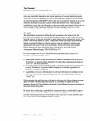
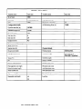
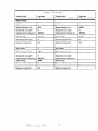
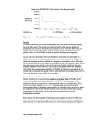
PRAIRIETM Guidance
A Watson, J W Clark and L S Fryer
Research Contractor:
AEA Technology plc
Environment Agency
Rivers House
Waterside Drive
Aztec West
Bristol
BS12 4UD
R&D Technical Report P68
Publishing Organisation
Environment Agency
Rivers House
Waterside Drive
Aztec West
Bristol
BS12 4UD
Tel: 01454 624400
Fax: 01454 624409
0 Environment Agency 1997
All rights reserved. No part of this document may be reproduced, stored in a retrieval
system, or transmitted, in any form or by any means, electronic, mechanical, photocopying,
recording or otherwise without the prior permission of the Environment Agency.
The views expressed in this document are not necessarily those of the Environment
Agency. Its officers, servants or agents accept no liability whatsoever for any loss or
damage arising from the interpretation or use of the information, or reliance upon views
contained herein.
Dissemination
Internal:
External:
status
Released to Regions
Released to Public Domain
Statement of Use
This report provides guidance, above and beyond that provided in the User Manual, on the
use of PRAIRIETM (Pollution Risk from Accidental Influxes to Rivers and Estuaries). The
guidance is designed to assist first-time or infrequent users in using the package in the
assessment and management of risks to potable water supplies and to the aquatic
environment.
Research contractor
This document was produced under R&D Project No 707 by:
AEA Technology plc
Thomson House
Risley
Warrington
Cheshire
WA3 6AT
Tel: 01925 232000
Fax01925254302
Environment Agency’s Project Manager
The Environment Agency’s Project Manager for R&D Project 707 was:
Mr Simon Halfacree - Environment Agency, Welsh Region
R&D Technical Report P68
Executive
Summary
PRAIRIETM, Pollution Risk from Accidental Influxes into Rivers and Estuaries, is a software
package developed by AEA Technology plc. It is designed to enable the assessment of risks to
water quality from chemical spills into rivers.
This Guidance document has been produced as an aid to occasional or first time users of
PRAIRDF who do not require the detailed information available in the PRAIRIETM ~6.01
User’s Guide (AEA 1993) or the modelling report (AEA 1996).
This document contains the bare essentials, i.e. sufficient information to run the code
successfully and obtain meaningful results, in the form of simple, step-by-step examples.
Guidance is also given on how to use the PRAIRIE TMdatabases to greatest effect and avoid
some potential pitfalls.
R&D Technical Report P68
R&D Technical Report P68
Contents
1 INTRODUCTION
5
2 WHEN TO USE PRAIRIEm
7
3 DETERMINISTIC
ASSESSMENT
9
4 PROBABILISTIC
ASSESSMENT
17
5 CHEMICAL
SINKS
23
6 FLOW AND DISPERSION
27
6.1 TRIBUTARIES
28
7 WATER QUALITY
8 GRAPHICAL
31
OUTPUT
9 MASS BALANCE
10 CONTACT
VALUES
35
ERRORS
37
NUMBERS
39
11 REFERENCES
41
Appendices
APPENDIX
1
R&D Technical Report P68
PRAIRIEW
DATA SHEETS
R&D Technical Report P68
Introduction
PRAIRIETM, Pollution Risk from Accidental Influxes into Rivers and Estuaries, is
a software package developed by AEA Technology plc. It is designed to enable
the assessment of risks to water quality from chemical spills into rivers.
PRAIRIETM has been designed to assist in managing the risk to selected targets
from accidental spills of chemicals, such targets include potable water abstraction
points, as well as valued aquatic ecosystems. A brief history of the programme of
work that has led to the development of the package is contained in the
introductory section of the PRAIRIETM ~6.01 User’s Guide.
From the beginning it was intended to develop a model which was simple to use
and yet permitted probabilistic risk assessments to be undertaken. Thus, the
mathematical model for dispersion is relatively straightforward. Although more
complex models do exist, these require considerably more input data and greater
computer resources than PRAIRIETM. PRAIRIETM was designed to be used by the
non-expert, whether an industrial user, consultant or field officer from the
regulatory authorities, and as such remains a simple, straight-forward computer
package which can be run with the minimum of input data.
There is always a compromise when developing such a package, between
providing detailed information on the available modelling capabilities, and
ensuring that the information supplied is tailored for the intended users. In order to
address these concerns a separate ‘modelling’ report has been produced (AEA
1996) which is available for those who wish to understand the modelling details.
The PRAIRIETM User’s Guide (AEA 1993) contains a great deal of information on
the key features of the package and the menu commands available to the user.
However, some users may require a less detailed document. This Guidance
document is designed as an aid to first-time or occasional users, containing the
bare essentials -sufficient information to run the code successfully and obtain
meaningful results. However, as you become more familiar with running the
package you may find reference to the User’s Guide or the modelling report
useful.
R&D Technical
Report P68
R&D Technical
Report P68
2
When to use PRAIRIETM
As stated above, PRAIRIETM was developed to enable the assessment of risks to
water quality from accidental chemical spills. However, there is more than one
way to assess risk and, as such, the package can be run in a variety of ways
depending on the exact question that the user wishes to answer. PRAIRIETM is
best used as part of a staged approach so that risks are identified and quantified in
an efficient and cost-effective manner.
The initial phase of any assessment should be a screening exercise, where any
chemical is analysed for the potential to cause significant adverse impact on water
resources in the event of an accidental release into a river system. Those chemical
hazards identified as being potentially significant, can then be assessed in more
detail taking into account on-site features which may mitigate against the severity
of any spill .This approach is consistent with the Environment Agency’s Rapid
Risk Assessment protocol which is designed to identify and assess priority risks in
a systematic way.
As part of a screening exercise it is expected that PRAIRIETM will generally be run
first in deterministic mode. Deterministic is a term used to describe a run that only
uses a single set of hydrological data and assesses only one chemical spill; it does
not include any allowance for the likelihood of the occurrence of either the chosen
flow conditions or the spill. A deterministic run can be used to calculate the
concentration of a chemical at any point downstream, following a spill from a
specified location. Comparing the chemical concentration with predefined water
quality standards (available as a database within PRAIRIETM) will enable the user
to make an informed judgement on the significance of the risk posed to the water
resource due to the spill.
If risks are considered to be significant following a deterministic assessment then
a more detailed probabilistic assessment may be undertaken. A probabilistic
assessment includes a run where neither spill characteristics nor river conditions
are fixed but are varied within a realistic envelope of values. Hydrological data are
taken from a database of annual flow statistics, supplied as part of PRAIRIETM for
selected rivers, whereas a range of spill scenarios can be specified by the user. In
this way an assessment can tell us the overall risks which the site poses to water
quality across the full range of on-site operations and environmental conditions.
As with any information, when to use PRAIRIETM is best illustrated by example.
The following sections contain examples of a simple deterministic run and a more
detailed probabilistic assessment for a fictitious manufacturing site located on the
River Dee in North Wales.
R&D Technical
Report P68
R&D Technical
Report P68
3
Deterministic
Assessment
A simple deterministic assessment of a site should be used to answer the
following type of question:
A manufacturing site, 104 km upstream of the mouth of the river Dee and 25
km upstream of a potable water abstraction point, stores 200 tonnes of
methanol in a single tank. If the methanol accidentally reached the river, for
example following catastrophic storage tank failure, would it pose a threat to
the potable water abstraction?
For this assessment we are interested in whether the potable water abstraction
point is likely to be compromised at any time. In the first instance it is best to
consider the worst case scenario and use conservative assumptions such as loss of
the complete chemical inventory to the river, low flow conditions and no
reduction in chemical concentrations due to environmental fate processes, e.g.
evaporation, oxidation etc.
It is obviously up to each user to refine the input data set, but, in the first instance,
the user may wish to use the following values for a screening assessment:
chemical sinks turned OFF, i.e. do not cross the on-screen Sinks box;
river under 95%-ile flow conditions (i.e. low flow conditions implying
relatively little dilution);
total loss of chemical inventory over 10 minutes (i.e. the rapid loss of
maximum pollutant).
The input set for this example is summarised on the following data sheet. Note
that although the data sheet has been designed to hold the maximum amount of
information, relatively little input data are actually necessary to complete this
screening run. A blank data sheet is contained in Appendix 1.
Configuration
The stretch of river to be modelled is defined on the configuration screen. It is
generally a good idea to start modelling the river a few kilometres upstream of the
spill site and finish just below the water abstraction point. The model requires that
the river be divided into mesh points but, unless you require a specific number,
two hundred mesh points is generally sufficient for most runs. The start and end
times of the run are also required and again, unless specifically required to differ,
the run can start at time zero and run for not more than 96 hours (PRAIRIETM will
accept longer runs but is not intended to model releases over longer time periods).
Finally, for our example, and for most runs, the output time for results is sufficient
at every half an hour.
R&D Technical
Report P68
Hydrology
The user is required to input a dispersion coefficient. The dispersion coefficient
cannot be varied along the length of the modelled river. This is generally the most
difficult parameter for which to acquire realistic input data and should be chosen
with care. Typical dispersion coefficients for the River Dee range from 3 m2/s to
65 m2/s (obtained from dye tracer experiments). Using a dispersion coefficient
from the lower end of the typical range will be conservative because the lower the
dispersion coefficient the less dispersion the pollutant plug undergoes in the river,
hence the peak concentration will be higher. For our example we are using 10
m2/s.
As a minimum, data on flow, velocity and water depth are required from upstream
of the spill site to downstream of the water abstraction point. Data for points
intermediate to these can be input if required. However, even the minimum data
requirement may be hard to fill and, in that case, it is considered conservative to
use available flow data from any point upstream of the spill site.
Please remember to click on the STORE button to input the hydrological
data for each location.
The Chemical
PRAIRIETM contains a database which includes an extensive list of potentially
hazardous chemicals. Methanol is included on this database and the user needs
only to select it from the on-screen listing. All relevant information on this
chemical is contained in the database which can then be read directly by
PRAIRIETM. Entries in the chemical database can be inspected and edited by the
user by pressing the View button.
If the chemical you are interested in is not contained on the database then choose
USERCHEMICAL from the list and enter information on the chemical (solubility
is the only essential requirement) via the View button. Some chemicals in the
database have an asterisk by them, these are the ones for which a concentration
designed to protect the quality of drinking water supplies has been suggested and
is contained in the PRAIRIETM water quality database (accessed during the
production of a graph).
The Spill
Following the selection of the chemical, the user must define the spill scenario, i.e.
the location of the spill site, the amount of chemical lost into the river and the time
period it is spilled over. As mentioned above it is suggested that, for a screening
run, the complete inventory of chemical is lost to the river over 10 minutes as a
uniform release. The facility to enter data for a more complex spill scenario, i.e. a
varying release rate, is available, however, this facility will be used in very few
cases as this detailed information is rarely available.
R&D Technical
Report P68
10
Remember to click on the CALCULATE
data.
button after entering the release
In addition, a background concentration for the spill chemical can be input where
the chemical is known to be present in the river under normal conditions.
PRAIRIETM adds the background concentration to the calculated spill levels in
order to provide a total chemical concentration profile.
R&D Technical
Report P68
11
R&D Technical
Report P68
12
PRAIRZETM DATA
Input data
Variable (units)
River Name
Input data
Variable (units)
~ DEE
Run Mode
DETERMINISTIC
Sinks
1 OFF
Configuration
SHEET
Mannings coeff (m)
Dispersion coeff (m*/s)
details
Upstream start dist (m)
Simulation length (m)
Release Details
No. mesh points
Release Frequency (/yr)
Start time (hr)
Background cone (mg/l)
End time (hr)
Upstream point of release
04
I
Output time (hr)
Environmental
data (complete only if sinks switched ON)
Wind speed (m/s)
0.2
I
I
Sunrise time (hi-)
Chemical
Cloud cover (tenth)
Chemical name
METHANOL
Daylight duration (hr)
Molecular weight
(alI details as in
PRAIRIETM database)
Temp (“C)
Solubility (mgjl)
PH
Henry’s constant
Organic carbon fraction
Oxidation rate const
Plant pigment cone (mfl)
Photolysis rate const
Dissolved carbon (mg/l)
Acid hydrolysis const
Molar oxidant (M)
Base hydrolysis const
Algae cone (mg/l)
Neutral hydrolysis
Suspended solid (mg/l)
R&D Technical
Report P68
13
details
I
PRAIRIEm
R&D Technical
Report P68
DATA
SHEET
14
Concentration of METHANOL vs Time Plot at 78919.6 metres
2500
+.t
2000
t
Concentration
1500
(mg4
+
+
1000 -500
Figure 1
/ Water Quality = 1.4
(HUMSNARL)
I
t
Example Deterministic
+.’ Dissolved
Assessment Results
Results
In order to decide if the above spill poses a significant risk to the abstraction point
or other chosen environmental target, i.e. what concentration of methanol can be
tolerated in the river, the maximum (peak) concentration at the target, in this case
the abstraction point, should be compared with the pre-defined water quality
value. For this purpose PIWIRIEW includes a database containing a range of
water quality values for an extensive list of chemicals. Where the purpose of the
assessment is to determine risks to an abstraction point then the water quality
value generally selected is the 24 hour suggested no adverse response level
(SNARL). The 24 hour SNARL is defined as the level of chemical in drinking
water which is considered safe to drink at normal consumption rates over 24
hours. Thus, in this example, in order to protect potable water supplies the
chemical concentration at the abstraction point should remain lower than the 24
hour SNARL for methanol (a value within the water quality database).
To display the results of the PRAIRll?
run select the Results option from the
File menu. You will need to wait a short time for the results to be read into an onscreen table. A graph such as that above is then obtained from the results table by
choosing Concentration vs. Time from the Plot menu and plotting the dissolved
chemical concentration. The SNARL value is selected from the water quality
database and the distance at which the concentrations are plotted is specified as
79000 m, i.e. the upstream distance to the water abstraction point from the mouth
of the river. The facility exists for the user to input a water quality value if, for
example, no value exists in the database or the user wishes to use an alternative
value.
From the graph produced in this example, automatically plotted at the nearest
mesh point to the water abstraction point, it is obvious that the peak concentration
R&D Technical
Report P68
15
of 2.3 g/l is massively greater than the SNARL value of 1.4 mg/l. From this we
can infer that the methanol storage facility, 25 km upstream of the water
abstraction point, has the potential to pose a significant threat to the water
abstraction and warrants a more detailed investigation.
But what if the assessment had resulted in peak concentrations at the abstraction
point just above or just below the SNARL value? In any risk management
decision making it is always important to bear in mind that the results from any
risk assessment are subject to some degree of uncertainty and that criteria (such as
exceedance of a SNARL level) on their own should not be the final arbiter in any
decision making; however, these factors need even greater recognition when risk
assessment results are close to any quantitative criterion.
R&D Technical
Report P68
16
4
Probabilistic
Assessment
Having conducted a deterministic assessment of the site, and decided that a more
detailed investigation is warranted, a probabilistic PRAIRIETM run will be
required. In this example a probabilistic assessment is being used to answer the
following question:
A manufacturing site, 104 km upstream of the mouth of the river Dee and 25
km upstream of a potable water abstraction point, stores 200 tonnes of
methanol in a single tank. The methanol can accidentally reach the river by a
number of routes, for example catastrophic tank failure, tank leakage, filling
and emptying operations etc. Taking into account all accident scenarios and
across the full range of potential river conditions, does the methanol storage
facility pose enough of a risk to drinking water supplies to merit the
introduction of further risk management measures?
For this assessment we are interested in the frequency with which the potable
water abstraction point is likely to be compromised and whether this frequency is
acceptable. Performing a probabilistic run means we are no longer required to use
only conservative assumptions and the range of spill scenarios and potential river
flows can be modelled. In this example the chemical sink terms will remain
switched OFF (chemical sinks will be dealt with separately in section 5).
The input data set for this example is summarised on the following data sheet. It
may seem surprising that no user-input flow data is required for this more detailed
assessment but that is because PRAIRIETM contains a hydrological database which
is accessed during a probabilistic run. Currently flow data is provided for three
rivers - the Dee, the Yorkshire Derwent and the Medway. Data for more rivers can
be included but only by contacting a ‘Super-User’ at AEA Technology plc (see
Section 10).
Configuration
Identical to previous deterministic run.
Hydrology
In addition to supplying a constant dispersion coefficient, the user must also input,
prior to conducting the run, the distance at which results are required. This is
known as the Upstream Monitoring Distance. In this example we are interested in
concentrations at the water abstraction point 25 km downstream from the
methanol store, i.e. 79 km upstream from the mouth of the river.
All other necessary hydrological data is supplied via the PRAIRIETM database.
R&D Technical
Report P68
17
The Chemical
Identical to previous deterministic run.
It is very rare that a site stores only one potentially hazardous chemical or that
only one potentially hazardous site exists upstream of a water abstraction point.
Therefore, in order to quantify the risk to drinking water supplies from a number
of upstream hazards, PRAIRIETM allows the user to model the release of up to five
different chemicals from any location within the defined river. Only during a
probabilistic run is the user allowed to select more than one chemical from the onscreen listing of the chemicals database. For this example, however, we are
concentrating on the loss of a single chemical from a single site.
The Spill
The information required to define the spill scenarios is the .same as for the
previous deterministic run with the added requirement of a spill frequency term.
Several sources of data are available to help assign failure frequencies to the ‘base
events’ which may result in a spill. These base events can range from hardware
failure to operator failure to external events, such as collisions, and the most
appropriate data source will vary accordingly. Some references and example
failure frequencies have previously been compiled in ‘A Guide to Risk
Assessment Methodologies’ NRA R&D Note 37 1.
For this example site we have identified three potential spill scenarios for
methanol which are detailed below:
l
l
l
catastrophic failure of tank releasing 200 tonnes of methanol into the river in
10 minutes. A generic failure frequency for mild steel, unpressurised tanks of
1x 1O4 yi’ has been identified;
incorrect tanker transfer operation leads to 20 tonnes of methanol reaching the
river in 30 minutes. A generic failure frequency for transfer operations of
7~10~~yr-’ could be predicted;
a guillotine cut in an overhead pipe on-site loses 20 tonnes of methanol to the
river over 30 minutes. A generic frequency for such a pipe failure could be
1.5~10-~ yi’.
When entering the spill data you will need to click on the <New> button between
spills to create a second and third data set. It is possible to model five spill
scenarios for each of five different chemicals from different locations upstream of
the water abstraction point.
Be aware that conducting a probabilistic assessment takes considerably longer to
run than a deterministic run. This is because the probabilistic assessment is
actually calculating numerous deterministic runs (one run for each possible spillflow combination) and amalgamating the results.
R&D Technical
Report P68
18
PRAIRZETM DATA
Input data
Variable (units)
I River Name
I Run Mode
I PROBABILISTIC
Sinks
Configuration
SHEET
Variable (units)
Mannings coeff (m)
Input data
I
Dispersion coeff (m*/s)
OFF
u/s Monitoring Point (m)
details
Upstream start dist (m)
Simulation length (m)
I No. mesh points
I Start time (hi-)
I 200
I 0
End time (hr)
24
Output time (hr)
0.5
Environmental
data (complete only if sinks switched ON)
Wind speed (m/s)
Sunrise time (hr)
Chemical
Cloud cover (tenth)
Chemical name
Daylight duration (hr)
Molecular weight
Temp (“C)
Solubility (mg/l)
details
I METHANOL
(alldetaikasin
PRAIRIEm
database)
Henry’s constant
I Organic carbon fraction
I Plant pigment cone (mg/l)
Oxidation rate const
I
Photolysis rate const
Dissolved carbon (mg/l)
Acid hydrolysis const
Molar oxidant (M)
Base hydrolysis const
Algae cone (mg/l)
Suspended solid (mg/l)
U/S
d/S
R&D Technical
Report P68
19
I
PRAIRIES
Variable (units)
Input data
DATA
SHEET
Variable (units)
Input data
Release Details
Spill Number
Spill Number
12
I
Release Frequency (/yr)
I lE-4
Release Frequency (lyr)
I 6.63-5
I
Background cone (mg/l)
0
Background cone (mg/l)
I 0
I
Upstream point of release (m)
104 000
mass lost (kg)
200 000
Start time of release (hr)
0
Duration of release (hr)
I 0.5
I
mass lost (kg)
I
I
Start time of release (hr)
I
I
Duration of release (hr)
Spill Number
Release Frequency (/yr)
Background cone (mgA)
Upstream point of release (m)
104 000
mass lost (kg)
Start time of release (hr)
I 0
Duration of release (hr)
Duration of release (hr)
R&D Technical
Urxtream uoint of release (m)
Report P68
20
Graph of the HUMSNARL Water Quality Value Being Exceeded
Frequency
(Per Year)
O.OOOO3
N x WQValue
Figure 2
Example Probabilistic
Assessment Results
Results
To obtain the results, as for the deterministic run, just select the Results option
from the File menu. The results are imported into a table and are displayed
graphically by selecting ‘Frequency Exceedance Curve’ from the Plot menu. In
order to calculate the curve you are also required to enter the relevant water
quality value, i.e. the SNARL in order to protect drinking water supplies.
As you can see, the results from a probabilistic assessment are presented in a
different format to the concentration profile of the deterministic run. Figure 2
shows the example result set plotted as a frequency exceedance curve. The units
on the horizontal axis on the figure are multiples of the water quality value; in this
case the chosen water quality value is the 24 hour SNARL and hence the axis
displays multiples of the SNARL. Any point on the graph shows the frequency
with which the corresponding multiple of SNARL is reached or exceeded. It is a
simple task to interpret this graph, what is more difficult is deciding what level of
risk to the drinking water quality is acceptable.
Figure 2 tells us that the frequency of an accidental spill at the methanol storage
facility resulting in a concentration equal to or greater than a SNARL at the
water abstraction point is approximately 4.1~10~~yi’. The frequency of an
accident at the site giving rise to a concentration equal to, or greater than, 83.6
times the SNARL value is 2.2~1O-~yr-‘. Whether these results illustrate an
unacceptable threat to drinking water supplies is a decision that can only be made
by comparison with locally defined criteria; such a decision would also require
appreciation of other issues, such as the costs associated with any risk
management measures.
Risk criteria for the protection of drinking water supplies on the river Dee have
previously been proposed to support the Dee Water Protection Zone application
under section 93 of the Water Resources Act 1991 and are illustrated in Figure 3.
R&D Technical
Report P68
21
The background to the criteria and their derivation are available in NRA R&D
Note 369. These criteria would require modification in order to suit local
circumstances in any other catchments. The application of such criteria has not
been formally adopted as part of Environment Agency policy (nor by the National
Rivers Authority, now part of the Environment Agency, for whom the criteria
were originally developed). It is not practicable to discuss the derivation of risk
criteria for individual catchments within this document but interested parties
should read the R&D Note.
Frequency
l.OE-01
=
l.OE-02
:
(per
year)
Intolerable
1 .OE-04
z
Acceptable
l.OE-05
1 .OE-06
I
l.OE-07
1 .OE-08
I
7 day
SNARL
Figure 3
I
24 hour
SNARL
1
Lb5
I
LC50
Proposed risk criteria for one site
The results from our example probabilistic run, presented in Figure 2, may be
plotted on, and compared with, the predefined criteria (as illustrated in Figure 3
for the protection of drinking water supplies on the river Dee). If the results from
the PRAIRIETM run fall into the acceptable region of the criteria graph then the
risks posed to the water abstraction point, by the methanol storage area, is found to
be acceptable. Therefore, no further action on the part of the site operators is
warranted on the basis of this comparison, although there may be reasons for
wishing to reduce risks further.
R&D Technical
Report P68
22
5
Chemical
Sinks
The examples in the previous sections were run with a minimum data set to
illustrate the ease with which PRAIRIlY can be used. To this end the chemical
sink terms were switched off for both examples. The chemical sinks are turned
ON by entering a cross into the chemical sinks box at the beginning of the
PRAIRllF
data input forms.
The term ‘chemical sink’ is used to refer to the variety of environmental fate
processes which may result in the partitioning, removal or transformation of the
spill chemical within the river, therefore leading to a reduction in dissolved
chemical concentrations. A brief description of the chemical sinks modelled in
PRAIRllF
is given in this section, however, much more detail is available in the
modelling report (AEA 1996).
The first process which an organic pollutant may undergo is dissolution. The
dissolved fraction becomes available to undergo further chemical reactions whilst
the undissolved fraction is transported downstream unaltered. The dissolved
component may be adsorbed onto organic particles suspended in the river water.
The particles with adsorbed chemical will disperse downstream. No subsequent
chemical reactions of adsorbed chemicals may occur. Chemical which is dissolved
but unadsorbed may undergo one or more of a number of chemical reactions.
PRAIRIETM can model volatilisation, hydrolysis, oxidation or photolysis.
As for organics, the first process that an inorganic pollutant must undergo is
dissolution. Undissolved chemical in transported downstream unaltered. The
dissolved species then undergo solvation and are partitioned between cation and
anion. Anions are assumed to be unreactive and are not removed from solution in
the PRAIRIIF
models. The dissolved cations may undergo chemical ionexchange reactions with suspended clays. The ion-exchanged particles will advect
downstream. The dissolved but non-exchanged cations stay in solution and
undergo advection and diffusion.
The choice of whether to include chemical sinks in your PRAIRIETM run
should be based on the availability of input data, the precision required by
the simulation and whether chemical effects are likely to be important for the
released chemical.
Although modelling the environmental fate of a chemical in the river would
reduce the conservatism inherent in a PRAIRIETM run with the sinks switched off,
modelling these chemical removal mechanisms require significantly more input
data. The majority of these input data are not easy to find and generally have a
degree of uncertainty associated with them.
R&D Technical
Report P68
23
If in doubt, leave them out! It is far better to be conservative and switch off
the chemical sinks, than use poor quality input data to model them.
The input requirements for sinks modelling are split into chemical information
and environmental characteristics. The chemical information, where available,
has been entered into the chemical database so that, when the user selects a spill
chemical from the on-screen list any available information is ready to be accessed
by PRAMEM. The database entries for all chemicals have primarily been taken
from the CHEMFATE database (1991) and occasionally an EPA report (EPA
1987). This information can be seen and edited by the user via the View button.
Note, however, that the available information is sparse and where no data were
available the removal mechanisms default to off. The full list of chemical-related
input required for complete sinks modelling is given on the PRAIRIETM data
sheets and includes the following:
Henry’s Constant (unitless)
PRAIRIETM uses Henry’s constant to determine the loss of chemical pollutant
from river water due to volatilisation.
Log Kow (witless)
PRAIRR? uses the octanol-water partition coefficient to determine the
equilibrium between material dissolved in the water and material adsorbed onto
suspended organic particles. This is another dynamic equilibrium and adsorbed
material may also be desorbed.
AKH, AKOH, AKN (Mm’hr.‘)
Hydrolysis of pollutants may proceed under neutral pH or may require catalysis
by acids or bases. PRAIRIETM therefore provides the option for three hydrolysis
rates for acid, base and neutral catalysis respectively.
AKS (hr-‘)
The surface photolysis of dissolved pollutants is modelled within PRAIRIETM as a
first order reaction. Literature values are sparse and have only been entered in the
database if clearly for direct photolysis.
AKOXMO (Mm’hi’)
The literature contains, for some pollutants, many oxidation rates. However, the
rates are highly dependent on the species with which the pollutant can react.
Values are only used for reactions with oxygen with a preference for values where
oxygen is in the excited singlet state IDOz.
The inputs required to model inorganic species are far fewer than for organics.
Dissolution is determined by the solubility (as for organic chemicals); all other
parameters required to determine the dispersion of inorganic pollutants are
calculated within PRAIRIEml. The user need only specify the ANION and
R&D Technical
Report P68
24
CATION names from an on-screen listing of species which are available to be
modelled by PRAIRIETM.
The additional environmental characteristics which are required as input in order
for PRAIRIETM to model chemical depletion mechanisms are detailed in Table 1,
along with a brief explanation as to why they are needed. If either of the chemical
or relevant environmental input data are missing for a particular removal
mechanism then that mechanisms cannot be modelled.
As can be seen in Table 1, the majority of environmental input data are required to
calculate photolysis. This is because photolysis is a complex process to model.
The various input parameters are required as they effectively reduce the energy of
the sunlight which reaches the pollutant and therefore reduce photolysis. It
follows, therefore, that if photolysis is not an important removal process for the
spill chemical, the majority of the environmental input data are not required to
model the spill.
It is worth making a note that although adsorption to suspended sediments is
modelled by PRAIRIE TM,the settling and resuspension of particulate matter is
not. PRAIRIlF
assumes that organic chemicals adsorb only onto the organic
fraction of suspended particles, i.e. organic carbon fraction times total suspended
solids. It is assumed for inorganic pollutants that all suspended solids are available
for ion-exchange.
Only when the sinks are switched on is the user required to input data about any
weirs along the modelled stretch of river. If you are modelling the Dee, Yorkshire
Derwent or Medway then the required information is held in a PRAIRIIF
database and comes up on-screen, otherwise data must be entered via the New
Weir button. The presence of weirs along the modelled stretch of river affects the
rate of volatilisation only and, therefore, if the spill chemical is not likely to
volatilise to any great extent there is limited advantage in spending time acquiring
the weir data. If volatilisation is important however, the higher the weir and the
less polluted the water, the higher the rate of volatilisation.
The inclusion of chemical sinks will increase computational run times,
R&D Technical
Report P68
25
Table 1 Environmental
Data Item (units)
Wind speed (m/s)
data required as input to model chemical sinks.
Sunrise time (hour)
Normal range of values
CO.5 (calm) to 12.5
(moderate) to >33
(Hurricane)
-4 (Jul) to -8.30 (Jan)
Cloud cover (tenths)
Oto 10
Daylight duration (hours)
- 17 (Jul) to -7.5 (Jan)
Temperature (deg C)
2 to 20
PH
6-9
Organic carbon fraction
0.0004 to 0.0729
Plant pigment
concentration (mg/l)
0.001 to 2
Dissolved carbon content
O-40
0.1 to 50
Molar oxidant
concentration (M)
0 to 1 (typically 1.OE-9)
Algae concentration
b-&U
Suspended solid
concentration (mg/l)
0 to 1000
Weirs
R&D Technical
extremely wide ranges
n/a
Report P68
26
Importance
required in the
calculation of
volatilisation onlv.
required in the
calculation of photolysis
only.
required in the
calculation of photolysis
onlv.
required in the
calculation of photolysis
only.
all rate coefficients are
adjusted to ambient
temperature.
required in the
calculation of hydrolysis
only.
required in the
calculation of adsorption
of organics to sediments.
required in the
calculation of photolysis
onlv.
required in the
calculation of photolysis
only.
required in the
calculation of oxidation
not required for any
sinks modelling in ~6.0 1.
required in the
calculation of adsorption
and nhotolvsis.
required in the
calculation of
volatilisation only.
6
Flow and Dispersion
In addition to the chemical behaviour of a pollutant in a river, there are two
important physical phenomena which are modelled by PRAIRIETM.
The first is the general tendency of the pollutant to flow downstream with the river
water. This phenomena is known as advection. The general user does not need to
be too concerned about the mechanics of advection. For deterministic
assessments, advection will be taken into account by the user input values for flow
and velocity. For probabilistic assessments, advection is automatically taken into
account through the hydrological data supplied with PRAIRIETM.
The second phenomena is the tendency of the spill profile to smear out as the
pollutant passes downstream. This phenomena is known as longitudinal
dispersion. The user has to tell PRAIRIETM how much dispersion is likely. This
is done in one of two ways, through an input on the River Specific Parameters
form, by either specifying the Longitudinal Dispersion Coefficient (units m2/s) or
the Mannings Roughness Coefficient (units m). These parameters predict
dispersion in different ways.
The longitudinal dispersion coefficient is used in instances where there is some
understanding of the hydrogeology of the river under consideration. The
Environment Agency, through a series of dye tracer experiments, have
characterised the behaviour (including dispersion) of many of the UK’s rivers
under a range of flow conditions. The Environment Agency’s hydrologists should
therefore be able to advise a PRAIRIETM user of suitable dispersion coefficients.
This is the preferred method of operation.
If there is no understanding of likely flow conditions then a PRAIRIl!? user
might decide to take account of dispersion through the input parameter known as
Mannings Roughness Coefficient. The Mannings Coefficient is a parameter
which attempts to predict the degree of dispersion according to the nature of the
river. The PRAIRIE help screen suggests ranges of input for rivers ranging from
clean and straight to winding and weedy.
Our experience of using PRAIRIE, coupled with original references where various
studies have been made to optimise the form of the Mannings equation, is that
there can be considerable differences between observed and predicted longitudinal
dispersion (both over- and under-estimates). We would therefore recommend the
user to directly input the longitudinal dispersion coefficient rather than rely upon
the Mannings coefficient.
R&D Technical
Report P68
27
When there are uncertainties surrounding an input value it is generally advisable
to set-up PRAIRIETM so that slight over-estimates of pollutant concentrations will
be made. This will ensure that conservative or pessimistic predictions are made so
that accident scenarios are not dismissed too early as presenting a low risk when
the opposite might better reflect reality. The larger the dispersion coefficient then
the greater will be the smearing out of a pollutant’s concentration profile, with the
consequence of predicting smaller pollutant concentrations. Therefore, if there is
doubt surrounding the choice of longitudinal dispersion coefficient or Mannings
coefficient, the user should err towards selecting smaller input values.
Finally, it should be remembered that PRAIRIETM uses the same value for the
longitudinal dispersion coefficient for all points along the river and, when running
probabilistic scenarios, for all flow regimes. Therefore, when running in the
probabilistic mode the user should input a dispersion coefficient most relevant to
low flow conditions if conservative predictions are wanted. (This consideration
does not apply to the Mannings coefficient which is continually adjusted since the
calculation is expressed in terms of the flow and depth, both of which vary in
either deterministic or probabilistic modes).
6.1
TRIBUTARIES
There are two basic scenarios where the presence of a tributary flowing into the
main river channel could affect the data input requirements to PRAIRIETM. In one
case, a tributary flow into the main river channel between a potentially hazardous
industrial site and a potable water abstraction point would affect the pollutant
concentrations in the main river channel. Secondly, a potentially hazardous site
may be located on a tributary to the main river channel from which the drinking
water supply is abstracted.
In the first case, the presence of a tributary will result in an increase in flow in the
main river and a consequent increase in dilution of any pollutant. The increase in
flow at the confluence of the tributary and river can be taken account of by
specifying additional hydrological information for points intermediate to the start
and end of the stretch of river to be modelled. For example:
A manufacturing site is located 104 km upstream of the mouth of the river
Dee and 25 km upstream of a water abstraction point. The Afon Bradley
flows into the Dee 4 km downstream of the manufacturing site.
The hydrology input for a PRAIRIETM run could, therefore, look like this:
R&D Technical
Report P68
28
Location
Distance (m)
u/s boundary
Confluence
Abstraction
d/s boundary
105 000
100 000
79 000
75 000
95%-ile flow
( m3/s)
8
9
9.5
9.5
Velocity (m/s)
Depth (m)
0.29
0.31
0.33
0.33
0.25
0.5
0.5
0.5
where all flows are recorded on the Dee itself.
Unfortunately the effects of the increased turbulence at the confluence of two
flows, and the attendant increase in dispersion which may be expected, cannot
currently be accounted for in PRAIRIE TM.As discussed above in section 6, only
one dispersion coefficient can be specified for the whole length of the modelled
river and it would not be conservative to use an artificially high coefficient in
order to take the effect of the tributary into account.
The second scenario, where the potentially hazardous site is actually located on a
tributary, can be dealt with in exactly the same way as above:
A manufacturing site is located on the Afon Bradley, 4 km upstream of the
confluence with the Dee. The confluence, 100 km upstream of the mouth of
the Dee, is 21 km upstream of a water abstraction point.
In this case the hydrological data input to PRAIRIIF
Location
Distance (m)
u/s boundary
Confluence
Abstraction
d/s boundary
105 000
100 000
79 000
75 000
95%-ile flow
( m3/s)
0.02
9
9.5
9.5
could resemble this:
Velocity (m/s)
Depth (m)
1
0.31
0.33
0.33
0.1
0.5
0.5
0.5
where the upstream boundary is on the Afon Bradley rather than the Dee.
Again, only one dispersion coefficient can be input and will be applied to the full
length of the modelled stretch of river. The user must be careful to ensure that the
value of the dispersion coefficient used will give results that err on the side of
caution. In this case, however, where the spill site is such a short distance up the
tributary relative to the modelled stretch of river, it would seem more appropriate
to use a dispersion coefficient applicable to the upstream end of the main river
channel rather than to the tributary.
R&D Technical
Report P68
29
R&D Technical
Report P68
30
7
Water Quality
Values
As illustrated in previous sections, PRAIRIETM generates results in the form of
pollutant concentration as a function of time and distance (deterministic runs) and
frequency of exceedance curves (probabilistic runs). In order to help the user
decide on what, if any, actions should be considered in the light of PRAIRIETM
predictions a database of water quality values is provided. A number of water
quality values exist which should be used to help the user to put PRAIRIETM
results into some perspective. It is up to the user to decide which is the most
appropriate water quality value to use and this will depend on which component of
the environment is the focus of the assessment, i.e. the protection of quality at a
drinking water abstraction point or at an environmentally sensitive location. The
use of water quality values must be in line with Environment Agency policy in
this area (where it exists).
In addition, environmental risk criteria are currently being developed within a
research project part funded by the Environment Agency. These criteria may be
available in the future to help PRAIRIETM users make decisions on the
significance of their results and, therefore, the requirement for any subsequent
actions.
The entries included in the database, where information was available, are:
HUMSNARL
(mg 1.‘) The 24 hour Suggested No Adverse Response Level
(SNARL) for Humans.
The 24 hour SNARL values contained in the database were derived by the
National Centre for Environmental Toxicology (NCET) on behalf of the NRA.
The SNARL is generally based on the best available toxicological information and
is defined as the level of chemical in drinking water which would be safe to the
public over 24 hours (but no longer) under normal water consumption rates.
Organoleptic considerations (taste and odour) are also taken into account when
deriving SNARLS. The lowest reported taste or odour threshold for a chemical in
drinking water is compared to the health-based SNARL and the lowest value
reported as the HUMSNARL in the database.
However, it must be recognised that some of the SNARLS included are
conservative and based on limited data sets. These SNARL data should not be
used for incident management without ensuring they are up-to-date and relevant in
a specific situation. The data included in the PRAIRIETM database are provided to
support its application in risk management and not reactive incident management.
R&D Technical
Report P68
31
Comparison of HUMSNARL levels with PRAIRIETM results is valuable in all
cases where the intention is to protect the quality of potable water supplies
from chemical hazards.
Where no SNARL is available in the database it is either because there were
insufficient data available at the time to set a level, or it was considered
inappropriate to set a SNARL, e.g. the chemical is a solid at room temperature.
TASTE (mg 1.‘)
The aqueous threshold concentration above which a significant proportion of the
population would detect the pollutant in their drinking water. However, for some
of the chemicals, the levels given are the most sensitive thresholds reported.
Current best estimates are supplied by NCET.
ODOUR (mg 1.‘)
The aqueous threshold concentration above which a significant proportion of the
population would be able to smell the pollutant in their drinking water. However,
for some of the chemicals, the levels given are the most sensitive thresholds
reported. Current best estimates are supplied by NCET.
The EC Directive 75/440/EEC (concerning the quality required of surface water
intended for the abstraction of drinking water in the Member States) provides
mandatory and guideline objectives for various chemicals in the water prior to
abstraction. These objectives are divided into three categories with reference to the
level of treatment that the water will receive before going to potable supply. In the
database these objectives are termed ECAl, ECA2 and ECA3.
ECAl (mg 1.‘)
The EC quality objective for water intended for potable supply after undergoing
only simple physical treatment and disinfection, e.g. rapid filtration and
disinfection.
ECA2 (mg 1.‘)
The EC quality objective for water intended for potable supply after undergoing
normal physical treatment, chemical treatment and disinfection, e.g.
prechlorination, coagulation, flocculation, decantation, filtration, disinfection
(final chlorination) .
ECA3 (mg 1.‘)
The EC quality objective for water intended for potable supply after undergoing
intensive physical and chemical treatment, extended treatment and disinfection,
e.g. chlorination to break-point, coagulation, flocculation, decantation, filtration,
absorption (activated carbon), disinfection (ozone, final chlorination).
R&D Technical
Report P68
32
ENVOBJ (mg 1.‘)
These are environmental quality objectives which are not specifically targeted at
potable water supplies nor the protection of water from accidental pollution, but
serve to raise or maintain the quality of all waters. The entries in the database have
been compiled from a combination of UK environmental quality standards (EQSs
from the DOE Circular 7/89 ‘Water and the Environment. The implementation of
European Community Directive on pollution caused by certain dangerous
substances discharged into the aquatic environment.‘) and EC environmental
quality objectives (EQOs from 86/280/EEC EC Directive on Limit Values and
Quality Objectives for Discharge of Certain Dangerous Substances included in
List I of the Annex to Directive 76/464/EEC). New and updated EQS values are
published intermittently and the PRAIRIETM database is unlikely to contain all the
available EQS data.
Comparison of PRAIRIETM results with ENVOBJ values is only relevant for
comparative guidance, indicating that EQWEQO compliance is not
compromised at a location downstream of a chemical hazard.
The following ecotoxicological data included in PRAIFUETM provide guidance on
each chemical’s toxicity to a range of organisms. It is, however, inadvisable to
interpret these data without appropriate expertise. It is not possible to determine
the validity of the quoted figures in a particular situation without considering the
source of the data. For example, there may be considerable differences between
the effect on the species exposed under test conditions and the potential effect on
species found in the receiving water.
LCSOFSH (mg 1.‘)
The best available 96 hour LC50 for fish species. The 96 hour LC50 is the
concentration that would result in the death of 50% of individuals exposed over 96
hours. A limited amount of this aquatic toxicity data is contained in the database.
ECSODAPH (mg 1.‘)
These values refer to the 48 hour EC50 for Duphnia (chosen as a representative of
riverine crustaceans). The use of Effects Concentration (EC), rather than lethal
concentration (LC), reflects the difficulty in distinguishing immobile
unresponsiveness from true lethality.
ECSOALG (mg 1.‘)
These are 72 hour EC5Os for algae. A standard 72 hour exposure test used to
determine the Effect Concentration for algae (chosen as a representative of
riverine plankton).
Comparison of PRAIRIETM results with the lowest of LCSOFSH, ECSODAPH
and ECSOALG is advisable if the intention is to protect the quality of an
environmentally sensitive site from chemical hazards.
R&D Technical
Report P68
33
Water quality values are not available for every chemical listed in the PRAIRDF
chemical database. An asterisk (*) by a chemical name on the on-screen list
indicates that a HUMSNARL value can be selected for that chemical during the
graphical output phase. However, the facility exists, for every spill chemical, for a
user to enter their own water quality value during the plotting of results.
Please note that a water quality value (whether selected from the database or
user input) is essential in order to plot the results from a probabilistic run.
R&D Technical
Report P68
34
8
Graphical
Output
Results from a run are imported into an on-screen table by selecting the Results
option from the File menu. The results table contains all the information necessary
to plot graphs. The table contains a large amount of information, which makes it
difficult to interpret quickly. However, if the user plots the information required
the values are extracted from the main body of the table and inserted into the Data
Extraction box on-screen. It is easier, and more accurate, to read off peak
concentrations from the Data Extraction box than to estimate them from the
graphs.
For a deterministic assessment three plot options are available:
concentration
concentration
3D Graph.
vs distance;
vs time;
A graph of concentration vs distance will illustrate the concentration profile within
the river at a time specified by the user. Concentration vs time will plot the change
in pollutant concentrations with time at a distance specified by the user (usually
the location of interest, e.g. at a water abstraction point). The 3D graph option
combines the concentration at time and distance information to give an illustrative
diagram of the pollutant plume as it travels along the river.
The user must specify at least one of dissolved, adsorbed or undissolved chemical
to be plotted on the graphs. Adsorbed will only be of any interest when the
chemical sinks are switched on, and undissolved when the chemical is present in
excess of its solubility in water.
The majority of users will find the concentration
distance the most useful graph to plot.
vs time profile at a specified
Probabilistic results are plotted as a frequency of exceedance graph (see section 4)
which is the only option available. A water quality value is essential for this
function and if not available via the PR41RIETM database must be input by the
user.
The results table also holds the mass balance statistics which can be used to
determine whether PRAIRIETM has produced results which are acceptable. This
topic is expanded on in the following section (section 9).
It is a very simple operation to plot a graph from the results table, this has been
demonstrated during the example assessments in sections 3 and 4. However, the
R&D Technical
Report P68
35
graphs may sometimes appear to have an secondary peak or ‘blip’ trailing the
main pollutant profile. For the majority, this problem is caused by a phenomenon
called upstream diffusion.
Upstream diffusion is a by-product of the methods used by PRAIRIETM to
calculate mathematically how a pollutant flows and diffuses along the river.
Upstream diffusion is an artificial phenomenon which arises when such numerical
methods are used to predict real physical effects. It is undesirable but
unavoidable. However, the inaccuracies that it introduces are usually
insignificant, and the phenomenon should not worry the user, so long as the blip is
not mistaken for the main pollutant peak.
The blip itself is caused by the estimation of gradients in pollutant concentrations
across mesh points. The gradients are then used to determine how much pollutant
should be transferred into the next mesh point downstream. The repeated effect of
the calculation along a length of river is that a ‘concentration ripple’ is produced,
with blips of decreasing intensity appearing on either side of the main peak. In
theory more than one blip could be seen on either side of the main peak but they
would be so small that they could not be seen by the naked eye.
There is little that the user can do to avoid the blip and, as said earlier, the errors
associated with them are so small as to be of little concern. The user should,
however, be aware of their existence so that they are not confused with the main
pollutant profile. It is possible for the PRAIRIETM graphics routines to plot the
secondary blip rather than the maximum pollutant concentration, especially if the
graph requested is near to the end of the modelled stretch of river. In this case it is
probable that the main peak has actually passed the end of the river and the
graphics routines have recognised the secondary peak as the only pollutant in the
river and therefore plotted it out. A secondary peak will be instantly recognised by
the very small scale associated with the concentration axis (typically down to lE13 mg/l!).
R&D Technical
Report P68
36
9
Mass Balance
Errors
Mass balance statistics are used as a check that PRAIRIETM has produced results
which are acceptable. A mass balance check ensures that the mass of pollutant
added to the river, as specified by the user’s release profile, is actually found
within the river (taking into account the mass which might have been lost through
various sink mechanisms). Sometimes the check shows that there is less mass in
the river than the user intended; this will result in a mass balance error if the
differences are sufficiently large.
The cause of the mass balance error is very similar to the cause of upstream
diffusion. The numerical algorithm which predicts how the pollutant flows and
diffuses within a river produces a ripple effect about the main peak. Two things
may happen as a result of the ripple: (i) it may go negative, effectively taking mass
out of the river; or (ii) it may diffuse upstream from the release point and off the
end of the modelled stretch of river, again with the effect that mass is taken out of
the river. Mass balance errors therefore arise because artificial methods are used
to model real-life situations.
Mass balance errors can be avoided by careful selection of inputs when setting-up
a PRAIRIETM simulation. It is good practice to ensure that the chemical is not
released into the first mesh point of the simulation - as a general rule of thumb, the
greater the distance (and hence meshes) between the upstream boundary and the
release point the better. If an unacceptable mass balance error occurs the problem
can be reduced or eliminated by increasing the number of meshes specified for the
simulation thereby effectively increasing the number of meshes between the
upstream boundary and the release point.
Mass balance errors caused by numerical upstream diffusion become increasingly
common when trying to simulate larger releases under conditions of low velocity
and high longitudinal dispersion. Under these conditions the dispersion element
of the calculation (which is responsible for moving the mass upstream as well as
downstream) can dominate the velocity component of the calculation (which
moves mass downstream). The result of which is that the released chemical
disperses upstream, and passed the upstream boundary, before the flow rate in the
river can move the pollutant downstream, thus appearing to remove mass from the
system.
The results of the mass balance calculations are shown in the lower right hand
corner of the results box. The intended (released) mass and the total dissolved,
adsorbed and undissolved mass of chemical within the river are clearly shown the user must however scroll down the page to reveal the percentage error and
suggestions of how to reduce this error.
R&D Technical
Report P68
37
The mass balance tile associated with probabilistic runs can be quite large. As
described previously, in probabilistic mode PRAIRIETM actually undertakes
numerous deterministic runs (one for each flow - spill scenario) and mass balance
statistics are calculated for each of the scenarios. The user should carefully scroll
through the mass balance information to ensure that none of the runs caused an
unacceptable error. It should be noted that it is the early runs for each spill
scenario in a probabilistic assessment that are most likely to give mass balance
errors since these (low velocity) runs are most likely to correspond with adverse
velocity-dispersion ratios.
R&D Technical
Report P68
38
10 Contact
Numbers
If you experience any difficulties in running PRAMEM, require additional copies
of the package or have any other queries, then help and advice can be obtained
from the PRAIRIEm Help Desk at AEA Technology plc.
The address and telephone number of the Help Desk is:
Software Help Desk
Customer Support Services
AEA Technology plc
Thomson House
Risley
Warrington
Cheshire
WA3 6AT
Telephone:
Facsimile:
-1-441925 254676
+44 1925 254677
For information on PRAIRD?
training courses, risk assessment and risk
management techniques, the derivation of risk criteria for use with PRAIRIE?,
on the use of risk criteria in general, enquiries should be addressed to:
Lynda S Fryer or Amanda Watson
AEA Technology plc
Thomson House
Risley
Warrington
Cheshire
WA3 6AT
Telephone:
Facsimile:
R&D Technical
+44 1925 254465
+44 1925 254570
Report P68
39
or
R&D Technical
Report P68
40
11 References
AEA (1993) PRAIRIE ~6.01 User’s Guide.
AEA (1996) Aqueous Pollution Modelling - Approaches used by PRAIRIETM.
Report No AEATCHEMFATE
Corporation.
(199 1) Environmental Fate Databases. Syracuse Research
EPA (1987) Processes, Coefficients and Models for Simulating Toxic Organics
and Heavy Metals in Surface Waters. EPA/600/3-87/015 (June 1987).
NRA (1995) Development of Risk Criteria for the Protection of Potable Water
Abstraction Points. R&D Note 369. Copies available from the Foundation for
Water Research, Allen House, Liston Road, Marlow, Bucks SL7 1FD.
R&D Technical
Report P68
41
R&D Technical
Report P68
42
Appendix 1
PRAIRIETM Data Sheets
CONTENTS
Deterministc Data Sheet
Probabilistic Data Sheet
R&D Technical
Report P68
43
R&D Technical Report P68
44
PRAIRIETM
Variable (units)
DATA
SHEET
Input data
Variable (units)
Input data
DETERMINL!STIC
Mannings coeff (m)
I
Dispersion coeff (m%)
I
River Name
Run Mode
Sinks
Configuration
details
Upstream start dist (m)
Simulation length (m)
Release Details
No. mesh points
Release Frequency (/yr)
I
Start time (hr)
Background cone (mg/l)
I
End time (hr)
Upstream point of release
Cm)
Output time (hr)
mass lost (kg)
Environmental
data
(comptetc when sinks switched ON only)
Start time of release (hr)
Wind speed (m/s)
Duration of release (hr)
Sunrise time (hr)
Chemical
Cloud cover (tenth)
Chemical name
Daylight duration (hr)
Molecular weight
Temp (“C)
Solubility (mg/l)
PH
Henry’s constant
Organic carbon fraction
Oxidation rate const
I
Plant pigment cone (mg/l)
Photolysis rate const
I
Dissolved carbon (mgll)
Acid hydrolysis const
I
Molar oxidant (M)
Base hydrolysis const
Algae cone (mg/l)
Neutral hydrolysis
Suspended solid (mg!l)
R&D Technical
Report P68
45
details
PRAIRIETM
DATA
SHEET
Input data
Variable (units)
Hydrological data at Start Time
Hydrological data at End Time
Upstream Boundary
Upstream Boundary
Flow (m3/s)
I
$y=
Velocity (m/s)
Depth 04
Downstream Bound&y
Downstream Boundary
Flow (m3/s)
I
1
Velocity (m/s)
Depth0-4
Intermediate distance/s
Intermediate distance/s
Flow (m3/s)
Velocity (m/s)
R&D Technical
I
Report P68
46
PRAIRIEm
Variable (units)
DATA
SHEET
Input data
Variable (units)
PROBABILISTIC
Mannings coeff (m)
Input data
I River Name
I
I Upstream start dist (m)
Simulation length (m)
Output time (hr)
Environmental
data (complete whl en sinks switched ON only)
Wind speed (m/s)
Chemical
details
Chemical name
Molecular weight
Solubility (mg/l)
Henry’s constant
Oxidation rate const
Photolysis rate const
Plant pigment cone (mg/l)
I Dissolved carbon (mg/l)
I Molar oxidant (M)
Acid hydrolysis const
Base hydrolysis const
Neutral hydrolysis
Algae cone (mg/l)
U/S
d/S
R&D Technical
Report P68
47
I
PRAIRIETM
R&D Technical
Report P68
DATA
SHEET
48
R&D Technical
Report P68
49