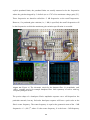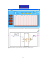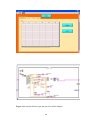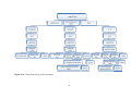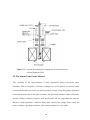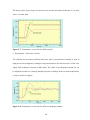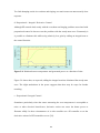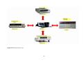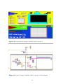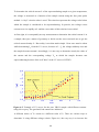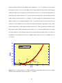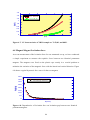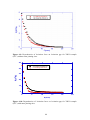
1
STUDYING MAGNETOTRANSPORT PROPERTIES OF SUPERCONDUCTORS USING LABVIEW by Huda Mahmoud Haddad Dr. Abdalla Obeidat Dr. Borhan A. Albiss Thesis submitted in partial fulfillment of the requirements for the degree of M.Sc in Physics At The faculty of graduate studies Jordan University of science and Technology June, 2010 STUDYING MAGNETOTRANSPORT PROPERTIES OF SUPERCONDUCTORS USING LABVIEW STUDYING MAGNETOTRANSPORT PROPERTIES OF SUPERCONDUCTORS USING LABVIEW by Huda Mahmoud Haddad Signature of Author …..……………….. Committee Member Signature and Date Dr. Abdalla Ahmed Obiedat (Chairman) …..……………….. Dr. Borhan A.Albiss (Co-Advisor) …..……………….. Dr. Maen Gharaibeh (Member) …..……………….. Dr. Abdul Raouf Al-Dairy (External Examiner, YU) …..……………….. June, 2010 DEDICATION To my Mother To my Brothers and Sisters And To My advisors Dr. Abdalla A. Obeidat and Dr. Borhan A. Albiss i ACKNOWLEDGMENTS I would like to thank my advisor Dr. Abdalla Obeideat for his support and for his supervision during the research, I am also indebted to him for his guidance in different fields specially in computational physics and programming and for sharing his knowledge and resources. I am grateful to my Co-advisor Dr. Borhan Albiss for his encouragement and support during the whole research project. He is one of the fewest teachers that you will never forget his way of doing science at high and well organized levels. I produce my deep thanks to the committee members; Dr. Maen Gharaibeh and Dr.Abdul Raouf Al-Dairy. I have the honor to discuss with them my thesis and receive their comments. Special thanks to Eng.Hazem Al-Rashaideh for his technical support and suggestion to have a complete work. My thanks to all my proffessors and doctors in the applied physics department at J.U.S.T specially Dr. Hasan al-Ghanem, Dr.Khalaf Abd Alazeez and Dr Mohammad Gharaibeh . Finally I'd like to say thanks to my friend Zeinab Ghadieh for supporting me through the research time. ii TABLE OF CONTENTS Title Page DEDICATION i ACKNOELDMENTS ii TABLE OF CONTENTS iii LIST OF FIGURES vi LIST OF TABLES viii ABSTRACT ix 1 Chapter One: Introduction 4 Chapter Two: Superconductivity 2.1 Brief History of Superconductivity 4 2.2 Applications of Superconductivity 11 Chapter Three: LabVIEW for Automated Test and Measurement 20 3.1 What is LabVIEW? 20 3.2 LabVIEW Program 21 3.3 Programming by LabVIEW 23 27 3.4 Virtual Instrumentation 28 3.5 Examples of Virtual Instruments (Vis) 3.5.1 Simple VI Design Patterns 28 3.5.2 General VI Design Patterns 29 3.6 Parallelism 30 3.7. Instrument I/O 31 32 3.8. Data Acquisition Chapter Four: Selected Examples on Interfacing Using LabVIEW 33 4.1 NI ELVIS II 33 34 4.1.1 Applications iii 35 4.1.2 NI ELVIS II Benchtop Workstation 4.1.3 NI ELVIS II Series Prototyping Board 35 4.1.4 NI ELVIS Functions 36 38 4.2 NI ELVIS Band-Pass Filter 41 4.3 GPIB 488.2 42 4.3.1 GPIB Signals 4.3.2 Types of Messages 43 4.3.3 Talkers, Listeners, and Controllers 43 4.3.4 Restrictions 44 44 4.4 LF Impedence Analyzer Chapter Five: Experimental Set-Up 52 5.1 Characteristic and Resistivity Measurement 52 54 5.2 The Linear Four Probe Method 5.3 Measurements procedure 57 5.4 PID (Propotional, Integral, Dervative ) Temperature Controller 58 5.4.1 PID Control, and its use with temperature 59 60 5.5 tuning a temperature controller 5.5.1 Types Of Temperature Controller 62 5.5.2 Types of Feedback Control 63 66 5.5.3 Third-Order Systems 5.6 Sources of Error and Measurement Considerations 66 5.7 I-V and R-T programs 68 5.8 Levitation Force 73 5.8.1 Levitation force Measurements Set-Up 75 Chapter Six: Results and Discussions 79 6.1 Sample preparation 79 80 6.2 Resistance-Temperature Measurements iv 6.3 I-V Characteristics 83 6.4 Magnet-Magnet Levitation force 86 87 6.5 Superconductor-Magnet Levitation Force Chapter Seven: Conclusions 91 References 94 Arabic Abstract 97 v LIST OF FIGURES Figure 2.1 2.2 2.3 2.4 2.5 2.6 2.7 2.8 2.9 2.10 2.11 3.1 3.2 3.3 3.4 3.5 3.6 3.7-a 3.7-b 3.8 3.9 4.1 4.2 4.3-a 4.3-b 4.4 4.5 4.6 4.7-a 4.7-b 4.8 4.9 4.10 4.11 4.12 4.13 4.14 5.1 5.2 DESCRIPTION Page Temperature dependence of the resistance for normal and superconducting states. Illustration of the functional dependence of the superconducting state with respect to magnetic field, temperature and current density. Type-I and type-II superconductors. Magnetic levitation force. YBCO Structure. Superconductor evolution through since 1900. Superconductor wires. High temperature-superconducting electric motors. The Yamanashi MLX01 MagLev train. SQUID SNS Junction. Wideband high Tc superconductor filter measured data. Tools, Controls and function pallets. LabVIEW Getting started window The front panel for addition & subtraction VI. The block diagram for addition & subtraction VI. Input and output functions terminals. LabVIEW Error list window. Simple VI Architecture. General VI Design Pattern. Parallel Loops front panel. Parallel Loop Design Pattern. NI ElVIS II hard ware. NI ELVIS II Soft Panel. Knobes. Elvis II right side. Protyping board Description. block diagram for band bass filter Figure: a) The electronic circuit for the banpass filter. (b) Amplitude and phase response curves for example bandpass filter. Note symmetry of curves with log frequency and gain scales. GPIB- CARD GPIB-USB-HS GPIB Cable Connecetor HP 4192A –computer interface Home page of hp4192A Calibration page Run & Acquire data front panel and part block diagram Analyzed Data page and part of its block diagram Flow chart for hp 4192A program Photo for the I-V characteristic and resistivity measurement system. Cryostat for making low temperature measurements in an 5 vi 6 7 7 10 11 14 15 17 18 19 23 24 25 25 26 27 29 29 31 31 34 34 35 35 36 38 40 41 41 42 46 47 47 49 50 51 53 54 5.3 5.4 5.5 5.6 5.7 5.8 5.9 5.10 5.11 5.12 5.13 5.14 5.15 6.1 6.2 6.3 6.4 6.5 6.6 6.7 6.8 6.9 6.10 external magnetic field. (a) Macro- and (b) micro-four-point probe method to measure electrical conductance. The distribution of current flowing through a superconductor specimen is also schematically drawn. Real photo for the 4-probe connections PID Block diagram Temperature vs. Time Auto tuning Temperature versus time for different gain Temperature versus time for different damping constant. Relation between temperature and generated power as a function of time Experiment set up Front panel for kethiley & lakeshore VI Part of kethiley & lakeshore block diagram Front Panel of R-T VI program Part of the Block diagram of The R-T VI Levitation experiment set-up Sample preparation procedures Resistance versus temperature for pure and nano-added YBCO sample in the temperature range (70 to 150 K). The critical temperatures criteria are shown Resistance versus Temperature curve for YBCO sample with nano-inclusion. Resistance versus Temperature curve for pure YBCO sample Example of I-V curves for the pure YBCO sample with different contacts using silver epoxy. The good and bad contacts are indicated. I-V characteristics of YBCO at different temperatures shown various voltage criteria used to determine critical current IC1, IC2 and IC3. I-V characteristics of YBCO sample at T=78,83, and 88 K. Dependencies of levitation force on levitation gap between two identical permanent magnets. Dependencies of levitation force on levitation gap for YBCO sample (ZFC) without nano pinning sites. Dependencies of levitation force on levitation gap for YBCO sample (ZFC) with nano pinning sites vii 55 56 59 61 64 64 65 70 71 71 72 73 76 80 81 82 82 84 85 86 86 88 88 LIST OF TABLES Table DESCRIPTION Page 4.1 GPIB signal description 42 4.2 Parameters measured by Display A and Display B 45 . viii ABSTRACT STUDYING MAGNETOTRANSPORT PROPERTIES OF SUPERCONDUCTORS USING LABVIEW By Huda Mahmoud Haddad The computer technology and the Internet have the potential to provide a highly interactive and powerful learning environment for physics disciplines. We have automated several advanced physics experiments using LabVIEW, the industry standard software used for data acquisition and instrument control. LabVIEW “virtual instruments”, coupled with data acquisition and control devices, were created to interface with a Keithley Current-Voltage source and sensitive Nanovoltmeter, PID Lake shore temperature controller, HP low frequency impedance analyzer, Band pass filter, stepper motor, Shimadzu digital balance and NI-ELVIS II bread board. The automation of these experiments permits the rapid and easy collection and analysis of data, facilitating the student’s exploration of the basic and advanced physics of these experiments. We will present examples of our virtual instruments, magneto-transport experimental set-ups for low and high temperatures, collected data sets and experimental results. The main focus of this work is to study the current-voltage characteristics, resistance-temperature measurements and the magnetic levitation force of YBCO high temperature superconductors. The temperature dependence of I-V characteristics and R-T curves for YBCO samples have been investigated using four-probe method. The magnetic levitation force for a magnet-magnet and superconductor-magnet systems have been also studied. The results were compared and discussed in terms of the relation between the critical current density and the pinning force in a superconductor. ix Chapter One: Introduction The processing and characterization of new or unconventional materials and devices used in high-tech industrial applications makes use of automated equipment for each single step in processing and characterization techniques. These techniques use stand-alone equipment with built-in microprocessors or application of specific microcontrollers, which are hardcoded or programmed to accomplish that particular process. If equipment for another process has to be automated then again a process of designing an entire stand-alone system takes place. The disadvantages of using such systems are: they are expensive to manufacture; it consumes a lot of time to program the devices for such systems; and the user has little control of the internal system. In today's rapidly changing environment, manufacturers want to be able to improve the processes continually. This can require being able to alter the monitoring and control of the individual process. To accomplish these changes, a generic approach for monitoring and control of processes and equipment is desired. The main emphasis of this work is to develop a methodology for automatic monitoring and control of all electronic devices in our superconductivity and magnetic measurements laboratory and other related labs at the physics department using readily available hardware and software while still providing tight control over the measurements sensitivity of all parameters for optimum productivity and time saving. The challenge is to achieve improved performance by monitoring and controlling parameters using readily available and modifiable systems. This can be done by using a data acquisition (DAQ) and control system with LabVIEW, a graphical programming language tool. Data acquisition is the process of bringing a real world signal, such as voltage, into the computer for processing, analysis, storage or other manipulation. Each 1 process is characterized by certain parameters like vacuum, pressure, light intensity, temperature, noise and RF power. Using a PC- based DAQ and control system run by LabVIEW, it is possible to control the equipm ent with a hardware and software system that can be easily understood and modified. LabVIEW can command DAQ boards in the computer to read analog input signals (A/D conversion), generate analog output signals (D/A conversion), read and write digital signals. So using a data acquisition system and generic LabVIEW code, that can be easy modified, automation of equipment for any process can be implemented instead of using embedded devices and stand alone automation[1-3]. The advantages of such a generic approach are that system monitoring and control are easier to understand and modify because of LabVEW's flexibility and ease of programming. Excellent control can still be maintained, over process parameters because of the real-time feedback control system. This system can be implemented without losing the integrity and the safety parameters of the equipment. Using LabVIEW controlled DAQ system for automation, has been realized and implemented on several devices available in our labs which are used for characterization of semiconductors, superconductors, polymers, magnetic materials and nanomaterials. In addition, we have also tested several devices available in the electronic workshop and digital electronic lab used for educational purposes for undergraduate students using NIELVIS provided from National Instruments [4-6]. In this work, the main emphasis was on building a LabVIEW controlled and automated set-up for studying the magneto-transport properties of YBCO superconductor prepared in our labs with various preparation conditions. The phenomenon of superconductivity is having a tremendous impact on the advancement of technology in many fields including medicine and electronics. It is expected to have more impact in the future of electric motors, power production and 2 transmission, transportation and communication systems, medical imaging, superconducting magnets and accelerators [7]. After a sample is synthesized, its superconductivity must be measured. Because superconductors only exhibit their phenomenal behavior at low temperatures, all testing is carried out in cryogenic surroundings under vacuum conditions. Traditionally, all measurements were painstakingly taken by hand; however, now measurements of temperature, applied current, and voltage are controlled, received, and interpreted by a computer with the help of LabVIEW. This leads to design a quite reliable system and methodology to utilize new software and hardware technology in promising field of high temperature superconductivity. In this project, after this introductory chapter, brief literature review, instrumentation and experimental results are discussed in the ongoing Chapters. Chapter 2 presents a brief review to the history of superconductivity, basic properties superconductor and their potential applications. Chapter 3 explains the approach for Automation. It discusses the requirements of DAQ Boards and External Interface Boards, along with the tools that have to be used in automation LabVIEW and NI-EVIS II. Chapter 4 explains the implementation of this approach to specific experimental set-ups such as: impedance analyzer and bass filter using NI ELVIS II. Chapter 5 describes experimental set-up such as: PID temperature controller, Voltage-Current Characteristics and resistivity measurements using d.c. four-probe method and levitation force set-up and other related techniques. The LabVIEW code used for automation is also explained for each set-up. Chapter 6 discusses the results obtained from various experiments and the merits of such an automation approach and its applications. In Chapter 7 we will draw our conclusions and future work. 3 Chapter Two: Superconductivity 2.1 Brief History of Superconductivity A large number of metals and alloys when sufficiently cooled down to temperatures nearing 0 K, the dc electrical resistivity abruptly drops from a finite value to one that is virtually zero and remains there upon further cooling. Materials that display this behaviour are called superconductors, and the temperature at which they attain superconductivity is called the critical temperature Tc. Super conductivity is a very old and exciting field discovered by H. Kammerlingh Onnes in 1911 [8]. He showed that dc resistivity in mercury disappeared altogether at the critical temperature Tc (≈4.2 K). Since its discovery in 1911, a great number of metals and alloys were found to exhibit this property. The critical temperature Tc varies from superconductor to superconductor but lies between less than 1 K and approximately 20 K for metals and metallic alloys. Recently, it has been demonstrated that some complex cuprate oxide ceramics have Tc in excess of 100 K [9]. The transition from the normal to the superconducting state phase is often sharp and the sharpness of superconducting state transition depends on the state and purity of the sample, but in favourable situations it can occur within a temperature interval of less than 0.001 K. The resistivity-temperature behaviour for superconductive and non superconductive materials is shown in Figure 2.1. Zero resistance of a superconductor implied transmission of current at any distance with no losses, the production of large magnetic fields because a superconducting loop could carry current indefinitely storage of energy. These applications were not realized because, as was quickly discovered, the superconductors reverted to normal conductors at a relatively low 4 current density, Jc, or in a relatively low magnetic field, called the critical field, Bc. The three material parameters, Tc, Bc and Jc, have become very important in the practical applications of superconductivity. Figure 2.1: Temperature dependence of the resistance for normal and superconducting states. Figure 2.2 shows schematically the boundary in temperature, magnetic field, and current density space separating normal and superconducting states. The position of this boundary will, of course, depend on the material. For temperature, magnetic field, and current density values lying between the origin and this boundary, the material will be a superconductive, outside the boundary conductions is normal. The discovery and development, in the 1950s and 1960s, of superconductors which can remain superconducting at much higher fields and currents lead to the production of useful superconducting magnets. Abrikosov in 1957 studied, the behaviour of superconductors in an external magnetic field and discovered that one can distinguish two types of materials type-I and type-II superconductors [10]. While type-I expels magnetic flux completely from its interior, type-II does it completely only at small fields and partially at higher external fields. Thus due to the formation of the mixed-state, these materials can sustain superconductivity even in higher magnetic fields higher than 10 Tesla. Type-II superconductors are therefore the ones that are of interest for most large scale applications. 5 Such high-magnetic field and large current carrying capability superconductors, which exhibits two critical fields Hc1 and Hc2 , are called ‘‘hard’’ or type-II superconductors. They passes from the perfect diamagnetic state at low magnetic fields to a mixed state and finally to a sheath state before attaining the normal resistive state of the metal. The upper critical field of type II superconductors tends to be two orders of magnitude or more above the critical fields of a type I superconductor. Therefore, it is the advent of the type II superconductor that has made possible the manufacturing of superconducting magnets of incredible strength. We must note that a type-I superconductive body, as exemplified by many pure metals, exhibits perfect diamagnetism (Meissner state) below Tc and excludes a magnetic field up to some critical field Hc, where upon it reverts to the normal state. Magnetic field dependence for type-I or ‘soft’ and type-II or ‘‘hard’’ superconductors are shown in Figure 2.3. Figure 2.2: Illustration of the functional dependence of the superconducting state with respect to magnetic field, temperature and current density. 6 Figure 2.3: Type-I and type-II superconductors. The diamagnetic effect that causes a magnet to levitate above a superconductor is a complex effect Part of it is a consequence of zero resistance and of the fact that a superconductor cannot be shorted out. The act of moving a magnet toward a superconductor induces circulating persistent currents in domains in the material. These circulating currents could not be sustained in a material of any finite electrical resistance. Figure 2.4: Magnetic levitation force. These circulating persistent currents form an array of electromagnets that are always aligned in such as way as to oppose the external magnetic field. In fact, a mirror image of the magnet is formed in the superconductor -- with a north pole below a north pole or a south pole below a south pole. If the magnet is moved or rotated, the "mirror image" of the magnet rotates with it. A disk magnet levitating over a superconductor may be spun rapidly about its longitudinal axis without affecting its levitation. Figure 2.4 shows that 7 diamagnetism is strong enough to levitate a magnet can only occur in a superconductor. For this reason, the "levitating magnet" test is one of the most accurate methods of confirming superconductivity. In 1950, Emanual Maxwell discovered the isotope effect in superconductors [11]. This experimental observation was an important key to the theoretical explanations of the mechanism of superconductivity. In the isotope effect, the critical temperature for many superconductors depends on the isotopic mass, indicating that lattice vibrations are involved in the superconductivity, and that the attractive coupling between electrons is through the lattice vibrations (i.e., phonon mediated). Thus the existence of isotope effect indicated that although superconductivity is an electronic phenomenon, it nevertheless depends in an important way on the vibrations of the crystal lattice in which the electrons move. The discovery of Josephson Effect in 1962 opened up exciting potential for the use of superconductors in measurement science and in high speed electronic devices [12]. According to Josephson, quantum tunnelling effects should occur when a supercurrent tunnels through an extremely thin layer (~ 10 Å) of an insulator. Josephson tunnelling of paired electrons through an insulating barrier is remarkable in that the tunnelling amplitude is that of an individual pair, despite the fact that the pairs comprise a correlated many body condensate. BCS (Bardeen-Cooper-Schriefer) theory of superconductivity explains most of the phenomena associated with it and provides the basis for our present understanding of superconductivity in ‘conventional’ low temperature superconductors, and to some extent plays a role of ‘reference’ theory in the on-going search or a correct description of superconductivity in the recently discovered high temperature superconductors (HTSCs) cuprates, doped fullerenes, MgB2 [13]. 8 Until 1986, the highest Tc observed for any superconductor was only 23.2 K in an alloy of niobium, aluminium and germanium. This meant that superconductors had to be cooled by liquid helium—an expensive and sometimes unreliable process. All this suddenly changed with the discovery of Bednorz and Muller of high temperature superconductivity in a new class of ceramic materials in 1986. More precisely, they found evidence for superconductivity around ~ 40 K in La2–x Mx CuO4 (M = Ba or Sr) ceramic. Bednorz and Muller’s discovery was the result of several years of extensive investigations on metal oxides, some of which had earlier been shown to be superconducting. It is noteworthy that superconductivity in oxides had been known for many years but with very low Tc. The end of 1986 and the beginning of 1987 were marked by synthesis of rare-earth metal oxides with the discovery of the YBa2Cu3O7 (YBCO) superconductor with a Tc of 93 K [14]. The perovskite (ABO3) structure of YBCO is shown in Figure 2.5. This was a significant breakthrough as it meant that for the first time the world has witnessed the existence of a superconductor with a Tc above that of liquid nitrogen (boiling point 77 K) which is much more abundant than helium, much less expensive, and liquid nitrogen cryogenic systems are less complex than systems using helium refrigeration. The ease of making Y Ba2 Cu3 O7 ceramics by mixing calcining and oxidizing the constituent powders permitted its investigation by many laboratories of the world. Early in 1988, Bismuth (Bi) and Tl cuprate oxides were discovered with Tc = 110 and 125 K respectively [15,16]. These new HTSC containing Bi and Tl may have some advantages over ceramic superconductors containing rare-earths. Since the critical current density increases as T/Tc decreases, a Tc far above the opening temperature of liquid nitrogen temperture (77 K) is advantageous. Moreover, the new materials are more stable than the rare-earth cuprate superconductors; they do not lose oxygen or react with water. The maximum value of Tc has now increased to 133 K for mercury based cuprate Hg Ba2 Ca2 Cu3O8+x .When this compound is subjected to high pressure ~ 30 G Pa, the onset of Tc 9 increases to 164 K (more than half way to room temperature) [17]. While Hg Ba2 Ca2 Cu3 O8 cannot be used in applications of superconductivity at such high pressures, this striking result suggests that values of Tc in the neighborhood of 160 K, or even higher, are attainable in cuprate oxides at atmospheric pressure. Several research groups have claimed even higher transition temperatures but none of them were reproducible or independently confirmed by other laboratories. The dramatic evolution of critical temperatures that have been observed since 1911 is illustrated in Figure 2.6 where the maximum value of Tc is plotted versus date. Figure 2.5: YBCO Structure. During the last ten decades, high quality polycrystalline, single crystal and thin film specimens of these superconducting materials have been prepared and investigated extensively world wide to determine their fundamental, normal and superconducting state properties. Although we now probably know more experimentally about this class of materials than any other, we still have so many unresolved issues in understanding the basic mechanisms of high temperature superconductivity. 10 Figure 2.6: Superconductor evolution through since 1900. 2.2 Applications of Superconductivity The phenomenon of superconductivity is having a tremendous impact on the advancement of technology in many fields including medicine and electronics. It is expected to have more impact in the future of electric motors, power production and transmission, transportation and communication systems. Accordingly, the call to develop superconducting materials is strong and will remain so as the technology improves and becomes less expensive. Discovering or developing a material which becomes superconducting at room temperature is the ultimate challenge in superconductivity. But with the uncertainty of this ever being achieved, the current focus of much of the research, development and commercialization of superconductors, is on YBCO. The reason so much effort has been put forth on researching and applying YBCO superconductors rather than alternative high-temperature superconductors (HTSC) is because it has some of the best superconducting properties and offers the potential for lower cost products. ( repeated from the third page on the introduction) Zero resistance and high current density have a major impact on electric power transmission and also enable much smaller or more powerful magnets for motors, generators, energy storage, medical equipment and industrial separations. Low resistance at high frequencies and extremely low signal dispersion are key aspects in microwave 11 components, communications technology and several military applications. Low resistance at higher frequencies also reduces substantially the challenges inherent to miniaturization brought about by resistive, or I2R, heating. The high sensitivity of superconductors to magnetic field provides a unique sensing capability, in many cases 1000x superior to today's best conventional measurement technology. Magnetic field exclusion is important in multi-layer electronic component miniaturization, provides a mechanism for magnetic levitation and enables magnetic field containment of charged particles. In addition to trying to develop new HTSC materials, researchers were also trying to fabricate materials with improved critical current densities (Jc). Current densities as high as (105 – 106 A/cm2) may be needed for applications such as magnets, motors, and electronic components. The HTSC are ceramics and have all the brittleness problems associated with nonsuperconducting ceramics. In addition Jc is not an intrinsic property of superconductors but is a function of the processing procedure. The rare-earth superconductors also have highly directional properties. Therefore, a crucial problem is to fabricate the material into a useful shape and still have sufficiently high Jc and mechanical strength for practical applications The field of electronics holds great promise for practical applications of superconductors. The miniaturization and increased speed of computer chips are limited by the generation of heat and the charging time of capacitors due to the resistance of the interconnecting metal films. The use of new superconductive films may result in more densely packed chips which could transmit information more rapidly by several orders of magnitude. Superconducting electronics have achieved impressive accomplishments in the field of digital electronics. Logic delays of 13 picoseconds and switching times of 9 picoseconds have been experimentally demonstrated. Through the use of basic Josephson Junctions scientists are able to make very sensitive microwave detectors, magnetometers, SQUIDs and very stable voltage sources [12]. 12 The use of superconductors for transportation has already been established using liquid helium as a refrigerant. Prototype levitated trains have been constructed in Japan by using superconducting magnets Superconducting magnets are already crucial components of several technologies. Magnetic resonance imaging (MRI) is playing an ever increasing role in diagnostic medicine. The intense magnetic fields that are needed for these instruments are a perfect application of superconductors. Similarly, particle accelerators used in highenergy physics studies are very dependant on high-field superconducting magnets. The recent controversy surrounding the continued funding for the Superconducting Super Collider (SSC) illustrates the political ramifications of the applications of new technologies [18]. New applications of superconductors will increase with critical temperature. Liquid nitrogen based superconductors has provided industry more flexibility to utilize superconductivity as compared to liquid helium superconductors. The possible discovery of room temperature superconductors has the potential to bring superconducting devices into our every-day lives. High-temperature superconductors are recent innovations from scientific research laboratories. New commercial innovations begin with the existing technological knowledge generated by the research scientist. The work of commercialization centers on the development of new products and the engineering needed to implement the new technology. Superconductivity has had a long history as a specialized field of physics. Through the collaborative efforts of government funded research, independent research groups and commercial industries, applications of new high-temperature superconductors will be in the not so distant future. Time lags however, between new discoveries and practical applications are often great. The discovery of the laser in the early 60's has only recently been appreciated today through applications such as laser surgery, laser optical communication, and compact disc players. The rapid progress in the field of 13 superconductivity leads one to believe that applications of superconductors are limited only by one's imagination and time. As you can see application of superconductors is only just a beginning. • Transmission Line Power transmission is loosely defined as the transfer of electric energy from one source to a load over conductors that carry relatively large current with lower Ohmic loss. The penalty is the need to keep the superconductor cold. Fortunately, the superconductor can support a very large current density, and so little material is needed for the conductor. The Figure below shows superconductor wires where the cables are composed superconducting, there is no resistance and very little loss of electricity. This transmission cable can carry 3-5 times the current of conventional power cables [19]. Figure 2.7: Superconductor wires. • Electric Motors The main advantage of using superconductors in electric motors is that they can create an air gap magnetic field without any losses. The performance advantages of a hightemperature superconductor motor over that of a conventional motor include the following: high power density than a conventional motor due to the large air gap magnetic field produced by the lossless high-temperature superconductor winding and higher efficiency 14 than a conventional motor due to the lossless superconductor winding and smaller motor size. The high temperature superconducting motors are much smaller, lighter and more efficient when compared to a conventional motor as it appears in the Figure below. Utilities and industry will be able to lower their electricity costs by using these motors. Figure 2.8: High temperature-superconducting electric motors • High Temperature Superconductor Transformers: It offers utilities and industry a highly efficient, lightweight, compact and environmentally friendly alternative to today’s oil-filled transformers. • Fault Current Limiters It can protect power transmission, cable and operating equipment from surges of excess electricity caused by lightening strikes, short circuits and power fluctuations. The high temperature superconductor coils in the fault current limiter control the high current burst just long enough for the circuit breaker to open. The advantage of using a superconductor in a fault current limiter is that the resistance zero when in the superconducting state, which is nearly all the time. • Super Fast Computer Chips Superconductor materials can switch from superconducting state to the non superconducting state in 10-12 sec, about 1000 times faster than silicon. The suggestion that computers made from superconductors might be 1000 times faster than computers based on silicon chip technology. 15 • Levitation Superconducting Magnetic Energy Storage Devices (SMES): Electric power plants face their peak demand from customers in the late afternoon, but have excess generated at night and stored for half a day. The power plant would be much more efficient. One way to store energy is to make a flywheel’s bearings. With hightemperature superconductors employed as bearings, the efficiency of flywheel energy storage can improve dramatically. The mechanism behind superconductive flywheel bearing is Meissner Effect. Superconductor can repel magnetic field and a magnetic material will stand away from a superconductor. Therefore, it is possible to build a bearing surface with absolute no contact between pieces. • Magnetic Levitation Vehicles Main mechanism is Meissner Effect. There is attractive force between electromagnets and a ferromagnetic guidway, which is called electromagnetic system and there is repulsion force between two parts, which is called electrodynamics system. Magnetic Levitation Vehicles can reach speeds of over 300 mph, Figure 2.9. This method of transportation could be used to connect cities, which are from 200 to 350-miles apart, relieving congested highways and airports. The superconducting magnetic coils on-board the train and on the sidewalls of the guide way provide levitation, keep the vehicle in the center of the guide way and propel the vehicles along the track. • Superconducting Magnets Superconducting magnets can be used in Nuclear Magnetic Resonance Imaging (NMRI/MRI) in hospital and in high-energy physics accelerators. MRI is a noninvasive technique for seeing inside the body, which uses no ionizing radiation. The superconductive magnetic coils are an important portion of this whole –body scanner. Since these coils are capable of producing very stable, large magnetic field strength of magnets. Conventional magnets cannot produce very high magnetic field, superconductors 16 can generate more than 10 T magnetic field. An important factor limiting the magnetic field of an accelerator is the difficulty of making tapes and wire. Figure 2.9: The Yamanashi MLX01 MagLev train. • Power Electronics The purpose of power electronics is usually to switch large currents without having any moving mechanical parts; a transistor that changes states from “on” to “off” is the heart of the device. Because high-temperature superconductors can switch from superconductive state to nonsuperconductive state in very short time, high-temperature superconductor are very good candidates for this application. • Magnetic field Sensors There are a great number of potential uses for new magnetic field sensing devices. The applications for these devices are widespread from simple compass based navigation systems to ultra sophisticated (SQUIDs) that probe the invisible human biological activities. Several magnetic sensors based on various principles have been developed with the specific requirements of each sensor being particular to its application. A number of different materials properties may be exploited in sensor application including magnetoresistance, giant magnetoimpedance, magnetoocaloric, magneto-optical, and magnetostrictation effects. Each of these effects will also have its own advantages and 17 disadvantages for a particular field sensing application and device structure, and each presently has its own obstacles to be overcome for full integration into new field sensing technologies. • Superconducting Quantum Interference Devices (SQUID) One practical use of superconductors is in detecting very small magnetic fields. Not only can superconductors be used to generate magnetic fields greater than 10 T (105guass), they can detect magnetic field below 10-14 T. this remarkable sensitivity is achieved by Superconducting Quantum Interference Devices (SQUIDs). The underlying principle of a SQUID is tunneling. A quantum-mechanical effect produces the Josephson Effect. In addition, SQUID can be used detect corrosion highly sensitive. One interesting application of SQUID is detecting biomagnetism. In the body, neurons and muscle fiber both generate current when they are activated. SQUID can be used to detect a magnetic signal generated by several neurons or muscle fibers. Magnetoencephalgraphy (MEG) is using SQUID technology to produce a map of brain's magnetic activity, which can be used for tumor diagnosis [20]. Figure 2.10: SQUID SNS Junction. 18 • High Temperature Superconductor Filters: Microwave resonators with extremely high quality factors result in the ability to make filters with very little insertion loss, even with multiple poles in the filter, or even when the filter bandwidth is extraordinarily narrow. When such filters are used in receiver front ends, it is possible to have maximum frequency selectivity and maximum receiver sensitivity at the same time. Conventional filter technologies sacrifice sensitivity when selectivity is increased. In contrast, filters made using superconductors provide the closest approximation to a perfect filter; namely, one that allows 100 percent of the desired signals to pass through and rejects 100 percent of the unwanted signals, Figure 2.11. Hence, such filters are ideally suited for rejecting out-of-band signals, particularly those that are very close in frequency to the desired band. Because of the unique properties of superconducting filters, the most appropriate applications for the technology are either to produce filters with extraordinarily steep skirts (extremely rapid fall-off in transmission outside the band of interest) or to produce filters that are extremely narrow in bandwidth. In either case, such filters can still have very low insertion losses. Figure 2.11 shows the measured response of an HTS filter designed for the wideband CDMA spectrum near 1.9 GHz. Figure 2.11: Wideband high Tc superconductor filter measured data. The attenuation in this filter is such that the rejection reaches 100 dB only 400 MHz from the band edge. Such a filter would be virtually impossible to make using conventional approaches, and in any case would have enormous losses if it were built at all. 19 Chapter Three: LabVIEW for Automated Test and Measurement 3.1 What is LabVIEW? LabVIEW, Labortary Virtual Instrument Engieering Workbench, is a graphical programming language that is manufactured by National Instruments and is typically used to automate data acquisition in research labs and industry [3]. To accompany the software, corresponding hardware must also be installed. Within the central processing unit of a computer, a General Purpose Interfacing Bus (GPIB) card is installed into the PCI slot. The GPIB card is the connection between GPIB-compatible instrumentation and the computer. The card uses "handshaking" to communicate between talkers, listeners, and the controller. This means that the computer acts as the controller and is able to tell an instrument to be either a talker (it "tells" the controller what value it's at) or a listener (the controller "tells" it what value to go to). The card coordinates these transfers of information [21]. LabVIEW is the connection between the GPIB card and the data from the experiment. LabVIEW program works through a GPIB card to control the instruments, take measurements, and organize the results. Automated data acquisition greatly decreases the amount of human error, can be left to run on its own, and can be run regardless of the skill or experience of the user. LabVIEW programming uses icons instead of lines of text to create applications. In contrast to text-based programming languages, where instructions determine program execution, LabVIEW uses dataflow programming where the flow of data determines execution. 20 In LabVIEW, you build a user interface by using a set of tools and objects. The user interface is known as the front panel. You then add code using graphical representations of functions to control the front panel objects. The block diagram contains this code. In some ways, the block diagram resembles a flowchart. You can purchase several add-on software toolsets for developing specialized application. All these toolsets integrate seamlessly in LabVIEW. LabVIEW is integrated fully for communication with hardware such as GPIB, VXI, PXI, RS-232, RS-485, and data acquisition control, vision, and motion control devices. LabVIEW also has built-in features for connecting your application to the Internet using the LabVIEW Web server and software standards such as TCP/IP networking and ActiveX. Using LabVIEW, you can create 32-bit compiled applications that give you the fast execution speeds for custom data acquisition, test, and control solutions. You also can create stand-alone executables and shared libraries, like DLLS, because LabVIEW is a true 32-bit compiler. LABVIEW contains comprehensive libraries for data collection, analysis, presentation and storage. It also includes traditional program development tools. You can set breakpoints, animate program execution, and single-step through the program to make debugging and development easier. LABVIEW also provides numerous mechanisms for connecting to external code or software through DLLS, shared libraries, ActiveX, and more. In addition, numerous add-on tools are available for a Variety of application needs [22]. 3.2 LabVIEW Program LabVIEW programs are called virtual instruments or VIs, because their appearance and operation imitate physical instruments, such as oscilloscopes and multimeters. Every VI uses functions that manipulate input from the user interface or other sources and display that information or move it to other files or other computers. A VI contains the following three components: 21 • Front panel: Serves as the user interface. The front panel is the user interface of the VI. You build the front panel with controls and indicators, which are the interactive input and output terminals of the VI, respectively. Controls are knobs, pushbuttons, dials, and other input devices. Indicators are graphs, LEDs, and other displays. Controls simulate instrument input devices and supply data to the block diagram of the VI. Indicators simulate instrument output devices and display data the block diagram acquires or generates. • Block diagram: Contains the graphical source code that defines the functionality of the VI. After you build the front panel, you add code using graphical representations of functions to control the front panel objects. The block diagram contains this graphical source code. Front panel objects appear as terminals on the block diagram. Additionally, the block diagram contains functions and structures from built-in LabVIEW VI libraries. Wires connect each of the nodes on the block diagram, including control and indicator terminals, functions, and structures • Icon and connector pane: Identifies the VI. You can use the VI in another VI .A VI within another VI is called a subVI. A subVI corresponds to a subroutine in text-based programming languages. LabView program also contains the following three types of pallet which give you the options you need to create and edit the front panel and block diagram: • Tools Palette The Tools palette is available on the front panel and the block diagram. A tool is a special operating mode of the mouse cursor. When you select a tool the cursor icon changes to the tool icon. Use the tools to operate and modify front panel and block diagram objects. • Controls Palette 22 The Controls palette is available only on the front panel. The Controls palette contains the controls and indicators you use to create the front panel. • Functions Palette The Functions palette is available only on the block diagram. The Functions palette contains the VIs and functions you use to build the block diagram [3]. The figure below shows the three types of pallets: Figure 3.1: Tools, Controls and function pallets. 3.3 Programming by LabVIEW In this section we will illustrate briefly how to program a simple VI and how to deal with LabVIEW environment and its features. LabVIEW program differs from text based programming languages which need specific commands to program. One who uses LabVIEW, needs to know the available functions and controls in addition to learn their properties and options also he should know the rules that must to be obeyed through the programming. LabVIEW first window called "Getting Started" window, figure 3.2, from here you can create a new application, open an existing application, show some help resources and view examples by LabVIEW. 23 Figure 3.2 : LabVIEW Getting started window You will begin with simply clicking on the blank VI, once you click, two windows appear The first window is the front panel, behind it is the block diagram. On the front panel; when you click the mouse right button, the control pallet will be brought up, so we can access the available controls and indicators. These include numeric objects such as gauges and knobs, Boolean indicators such as buttons in different types, text controls and indicators, graphs, charts, arrays, tables, clusters and more. On the Block diagram where you develop your codes, clicking on the mouse right button makes the access to the function pallet, where all the LabVIEW functions found. These include structures for while loop and for loop, functions for simple math, arrays, Boolean logic, signal analysis and more. The first step on programming after planning is to put your controls and indicators which you need in the front panel, again controls are input elements where you can adjust the values or text. Indicators are output elements, which is used to indicate values, text or 24 graphs. Figure 3.3 shows the front panel for a simple VI which add two numbers and subtract them. Here we placed two numeric controls and two numeric indicators. Figure 3.3: The front panel for addition & subtraction VI. In the block diagram, An icon appears for each control and indicator there we need to add and subtract the two numbers stored in the controls and display the answer in the indicators, So the two functions (Add and subtract) are used to do this process and wires used to connect between controls, functions and indicators guarantee the data flowing through the VI. Figure 3.4 shows the block diagram for this example. This diagram executes the two numbers adding and subtracting. Figure 3.4: The block diagram for addition & subtraction VI. The control icons or functions in the block diagram have tow kind of terminals input terminals and output terminals. Figure 3.5 shows an example for such these terminals. Usually the terminals on the left side are input terminals and the terminal on the right side are output terminals. 25 Figure 3.5: Input and output functions terminals. You can run the VI, from the front panel either the block diagram, by clicking the run (white) arrow on the tool bar which will be changed to the black arrow as following . Errors in LabView are shown up without necessary to run the program, for example, if you wire to terminals have different types it will show the run wire as a broken wire. If you did something in the right way you will see a check mark on the tool bar. If there other mistakes such as unwired terminal, the run arrow will be converted to a broken arrow . If you click on the broken arrow you can see window that include a brief description about the errors as in Figure 3.6. Clicking on the "Show Errors'' button locates the errors position. An Interesting feature in the LabVIEW programming language, that there is a possibility to follow the program logically in the case that you want to see how the VI works or to look out for logical errors. This can be achieved by running the VI under highlight execution . It allows you to see how exactly the data flow from terminal to terminal with numbers evaluation at each node and each loop iteration. 26 Figure 3.6: LabVIEW Error list window. 3.4 Virtual Instrumentation Virtual instrumentation combines hardware and software with industry-standard computer technologies to create user-defined instrumentation solutions. National Instruments specializes in developing plug-in and distributed hardware and driver software for data acquisition (DAQ), IEEE 488 (GPIB), PXI, serial, and industrial communications. The driver software is the application programming interface to the hardware and is consistent across National Instruments LabWindows™/CVI™, and application Measurement software, Studio. These such as platforms LabVIEW, deliver the sophisticated display and analysis capabilities that virtual instrumentation requires. You can use virtual instrumentation to create a complete and customized system for test, measurement, and industrial automation by combining different hardware and software components. Many instruments are external to the computer and do not rely on a computer to take a measurement. By connecting instruments to a computer, you can programmatically control and monitor the instruments and collect data that you can process 27 further or store in files. You can install some instruments in a computer similar to generalpurpose DAQ devices. These internal instruments are called modular instruments. Regardless of how you connect to an instrument, the computer must use a specific protocol to communicate with the instrument. How the computer controls the instrument and acquires data from the instrument depends on the type of the instrument. GPIB, serial port, and PXI are common types of instruments. Like general-purpose DAQ devices, instruments digitize data, but they have a special purpose or are designed for a specific type of measurement. For standalone instruments, you generally cannot modify the software that processes the data and calculates the result because the software usually is built into the instrument. Because modular instrumentation uses software running on standard PC technology, you can more easily modify the behavior of these instruments. For example, with some digital multimeter modular instruments, you can program the instruments to acquire a buffer of data at a high rate of speed, much like an oscilloscope [3]. 3.5 Examples of Virtual Instruments (Vis) LabVIEW includes hundreds of example VIs you can use and incorporate into your own VIs. You can modify an example to fit your application, or you can copy and paste from one or more examples into your own VI. 3.5.1 Simple VI Design Patterns When performing calculations or making quick lab measurements, you do not need a complicated architecture. Your program might consist of a single VI that takes a measurement, performs calculations, and either displays the results or records them to disk. The simple VI design pattern usually does not require a specific start or stop action from the user. The user just clicks the Run button. You can convert these simple VIs into subVIs that you use as building blocks for larger applications. Figure 3.7-a, displays the block diagram of the simple VI architecture for determining the warning level. This VI performs 28 a single task—it determines what warning to output dependent on a set of inputs. You can use this VI as a subVI whenever you must determine the warning level. Note that this VI contains no start or stop actions from the user. In this VI all block diagram objects are connected through dataflow. You can determine the overall order of operations by following the flow of data. For example, the Not Equal function cannot execute until the Greater Than or Equal, the Less Than or Equal, and both Select functions have executed. 3.5.2 General VI Design Patterns A general VI design pattern has three main phases. Each phase may contain code that follows another type of design pattern. The three main phases include the following: Startup This phase initializes hardware, reads configuration information from files, or prompts the user for data file locations. Main Application This phase consists of at least one loop that repeats until the user decides to exit the program or the program terminates for other reasons such as I/O completion. Shutdown This phase closes files, writes configuration information to disk, or resets I/O to the default state. Figure 3.7-a shows a simple VI Architecture and Figure 3.7-b, shows the general VI design pattern. Figure 3.7 -a: Simple VI Architecture Figure3.7-b General VI Design Pattern In Figure 3.7 b, the error cluster wires control the execution order of the three sections. The While Loop does not execute until the Start Up VI finishes running and returns the error 29 cluster. Consequently, the Shut Down VI cannot run until the main program in the While Loop finishes and the error cluster data leaves the loop. Most loops require a Wait function, especially if that loop monitors user input on the front panel. Without the Wait function, the loop might run continuously and use all of the computer system resources. The Wait function forces the loop to run asynchronously even if you specify 0 milliseconds as the wait period. If the operations inside the main loop react to user inputs, you can increase the wait period to a level acceptable for reaction times. A wait of 100–200 ms is usually good because most users cannot detect that amount of delay between clicking a button on the front panel and the subsequent event execution. For simple applications, the main application loop is obvious and contains code that follows the Simple VI design pattern. When the program includes complicated user interfaces or multiple tasks such as user actions, I/O triggers, and so on, the main application phase gets more complicated. 3.6 Parallelism Parallelism is a way to execute multiple tasks at the same time. To discuss parallelism, consider the example of creating and displaying two sine waves at different frequencies. You place one sine wave in a loop and the second sine wave in a different loop. A challenge in programming parallel tasks is passing data among multiple loops without creating a data dependency. For example, if you pass the data using a wire, the loops are no longer parallel. In the (multiple sine wave example) you may want to share a single stop button between the loops, as shown in Figure 3.8. Some applications require the program to respond to and run several tasks concurrently. One way of designing the main section of this application is to assign a different loop to each task. For example, you might have a different loop for each button on the front panel and for every other kind of task, such as a menu selection, I/O trigger, and so on. Figure 3.9, shows this parallel loop design pattern. 30 Figure 3.8: Parallel Loops front panel. Figure 3.9 : Parallel Loop Design Pattern. This structure is straightforward and appropriate for some simple- menu type VIs, where you expect a user to select from one of several buttons that perform different actions. The parallel loop design pattern lets you handle multiple, simultaneous, independent tasks. In this design pattern, responding to one action does not prevent the VI from responding to another action. For example, if a user clicks a button that displays a dialog box, parallel loops can continue to respond to I/O tasks. 3.7 Instrument I/O This section introduces you to the basic concepts on how to use LabVIEW to acquire data from instruments controlled by GPIB, VXI, RS-232, and other hardware standards. LabVIEW communicates with most instruments through instrument drivers, which are 31 libraries of VIs that control programmable instruments. LabVIEW instrument drivers simplify instrument control and reduce test development time by eliminating the need to learn the low-level programming protocol for each instrument. Instruments obey a set of commands to respond to remote control and requests for data. When you use LabVIEW instrument drivers, you run intuitive, high-level command VIs, such as the Read DC Voltage VI for a digital multimeter or the Configure Time Axis VI for a digital oscilloscope. The driver VI you call automatically sends the appropriate instrument-specific command strings to the instrument. The foundation for LabVIEW drivers is the VISA (Virtual Instrument Software Architecture) VI library, a single interface library for controlling GPIB, VXI, RS-232, and other types of instruments. Drivers using VISA are scalable across instrument I/O interfaces. 3.8 Data Acquisition This section describes you how to use LabVIEW with general purpose data acquisition (DAQ) hardware. If you use only stand-alone instruments and control them with GPIB, VXI, or serial standards, refer to the Instrument I/O section of this chapter. Use the DAQ Solution Wizard If you are using DAQ hardware, you must configure analog input, analog output, digital input, or digital output channels. You can launch the DAQ Channel Wizard from the DAQ Solution Wizard to configure the channels. Then you can generate a DAQ solution from the Solutions Gallery [22]. Configure Analog Input Channels: The DAQ Solution Wizard guides you through naming and configuring analog and digital channels using the DAQ Channel Wizard. The DAQ Channel Wizard helps you define the physical quantities you are measuring or generating on each DAQ hardware channel. It queries for information about the physical quantity being measured, the sensor or actuator being used, and the associated DAQ hardware. 32 Chapter Four: Selected Examples on Interfacing Using LabVIEW 4.1 NI ELVIS II The National Instruments Educational Laboratory Virtual Instrumentation Suite II (NI ELVIS II) is a LabVIEW and computer based design and prototyping environment. NI ELVIS II consists of accustom-designed bench top workstation, a prototyping board, a multifunction data acquisition device, and LabVIEW based virtual instruments [5]. This combination provides an integrated, modular instrumentation platform that has comparable functionality to the DMM, Oscilloscope, Function Generator, and power Supply found on the laboratory workbench. The NI ELVIS II Workstation can be controlled either vi manual dials on the stations front or through software virtual instruments. The NI ELVIS II software suite contains virtual instruments that enable the NI ELVIS II work station to perform functions similar to a number of much more expensive instruments. One can use NI ELVIS II in engineering, physical sciences, and biological sciences laboratories. The suite offers full testing, measurement, and data logging capabilities .The environment consists of the following two components [5]: 1. Bench top hardware workspace for building circuits, shown in Figure 4.1. 2. NI Elvis software interface consisting of twelve soft front panels (SFP) instrument, figure 4.2. The soft panels are: 33 • Digital Multimeter (DMM) • Oscilloscope (Scope) • Function Generator (FGEN) • Variable Power Supply (VPS) • Bode Analyzer • Dynamic Signal Analyzer (DSA) • Arbitrary Waveform Generator (ARB) • Digital Reader (DigIn) • Digital Writer (DigOut) • Impedance Analyzer • Two –wire Current-Voltage Analyzer • Three –wire Current-Voltage Analyzer Figure 4.1 : NI ElVIS II hard ware Figure 4.2 : NI ELVIS II Soft Panel 4.1.1 Applications NI ELVIS II SFP instruments, such as the Bode Analyzer and Dynamic Signal Analyzer, offer instructors an opportunity to teach advanced courses in signal analysis and processing. 34 Mechanical engineering students can learn sensor and transducer measurements, in addition to basic circuit design by building custom signal conditioning. Students can install custom sensor adapters on the prototyping board. For example, installing a thermocouple jack on the prototyping board allows robust thermocouple connections [4]. The programmable power supply can provide excitation for strain gauges use in strain measurement. Physics students typically learn electronics and circuit design theory. NI ELVIS II provides these students with the opportunity to implement these concepts. For example, physics students can use NI ELVIS II to build signal conditioning circuits for common sensors such as photoelectric multipliers or light detector sensors. 4.1.2 NI ELVIS II Bench top Workstation NI ELVIS II hardware contains Bench top Workstation and Series Prototyping Board The workstation control panel provides easy-to-operate knobs for the variable power supplies and function generator, figure 4.3 –a, and offers convenient connectivity and functionality in the form of BNC and banana-style connectors, shown in figure 4.3 –b, to the function generator, scope, and DMM instruments at the right side of the bench top. Figure 4.3-a: knobes Figure4.3-b: Elvis II right side 4.1.3 NI ELVIS II Series Prototyping Board This section describes the NI ELVIS II Series Prototyping Board and how to use it to connect circuits to NI ELVIS II. The NI ELVIS II Series Prototyping Board connects to the 35 bench top workstation. The prototyping board provides an area for building electronic circuitry and has the necessary connections to access signals for common applications. Figure 4.4 shows the prototyping board with a brief description. You can use multiple prototyping boards interchangeably with the NI ELVIS II Bench top Workstation, Removing it from the bench top workstation. You can use the prototyping board connector to install custom prototype boards you develop. This connector is mechanically the same as a standard PCI connector. Figure 4.4: Protyping Board Description 4.1.4 NI ELVIS Functions. NI ELVIS II performs functions similar to a number of real instruments, which are used in common labs. ELVIS hardware and software integrated to gather to serve multi function as described below. DMM The primary DMM instrument on NI ELVIS II is isolated and its terminals are the three banana jacks on the side of the bench top workstation. For DC Voltage, AC and COM 36 Voltage, Resistance, Diode, and Continuity Test modes, use the V connectors. For DC Current and AC Current modes, use the A and COM connectors [5]. For easy access to circuits on the prototyping board, you can use banana-to-banana cables to wrap the signals from the user-configurable banana jacks to the DMM connectors on the bench top workstation Oscilloscope The two oscilloscope channels are available at BNC connectors on the side of the input impedance and can bench top workstation. These channels have robust 1 M be used with 1X / 10X attenuated probes. You can also use high-impedance Analog Input channels <AI 0..7> available on the prototyping board. Function Generator (FGEN) The function generator output can be routed to either the FGEN/TRIG BNC connector or the FGEN terminal on the prototyping board. A +5 V digital signal is available at the SYNC terminal. The AM and FM terminals provide analog inputs for the amplitude and frequency modulation of the function generator output [5]. Power Supplies The DC power supplies provide fixed output of +15 V, –15 V, and +5 V The variable power supplies provide adjustable output voltages from 0 to +12 V on the SUPPLY+ terminal, and 0 to –12 V on the SUPPLY– terminal .All power supplies on NI ELVIS II are referenced to GROUND [5]. Bode Analyzer The Bode Analyzer uses the Function Generator to output a stimulus and then uses analog input channels AI 0 and AI 1 to measure the response and stimulus respectively. 37 4.2 NI ELVIS Band-Pass Filter In circuit theory, a filter is an electrical network that alters the amplitude and/or phase characteristics of a signal with respect to frequency. Ideally, a filter will not add new frequencies to the input signal, nor will it change the component frequencies of that signal, but it will change the relative amplitudes of the various frequency components and/or their phase relationships. Filters are often used in electronic systems to emphasize signals in certain frequency ranges and reject signals in other frequency ranges. Such a filter has a gain which is dependent on signal frequency. There are five basic filter types (bandpass, notch, low-pass, high-pass, and all-pass). The filter used in this section as an example of bandpass filters. The number of possible bandpass response characteristics is infinite, but they all share the same basic form [23]. There are applications where a particular band, or spread, or frequencies need to be filtered from a wider range of mixed signals. Filter circuits can be designed to accomplish this task by combining the properties of low-pass and high-pass into a single filter. The result is called a band-pass filter. Creating a bandpass filter from a low-pass and high-pass filter can be illustrated using block diagrams: Figure 4.5 Figure 4.5: Block diagram for band bass filter. 38 The Band Pass filter demonstrates how Op Amps can be used to filter signals. The experiment allows for monitoring the filer in three locations—after the high pass stage, after the gain stage, and after the low pass stage for the final result [24]. The experiment uses the NI ELVIS Oscilloscope, Function Generator, and Bode Analyzer instruments. The high pass filter has a frequency response of: fo = 1 1 = ≈ 132.6Hz 2π R 2 R 3C 1C 3 2π 1.2k ∗1.2k ∗1μ ∗1μ The gain stage has a gain of: R4 ⎞ ⎛ ⎛ 10k ⎞ Vout = ⎜ 1 + ⎟ Vin = ⎜1 + ⎟Vin ≈ 11Vin R5 ⎠ 1k ⎠ ⎝ ⎝ Figure 4.6-a shows the input and output frequencies. Also the curves of gain vs. frequency and phase vs. frequency are plotted and commonly used to illustrate filter characteristics. The magnitude of the transfer function has a maximum value at a specific frequency (ω0) between 0 and infinity, and falls off on either side of that frequency. A filter with this general shape is known as a bandpass filter because it passes signals falling within a relatively narrow band of frequencies and attenuates signals outside of that band. The range of frequencies passed by a filter is known as the filter's passband. Since the amplitude response curve of this filter is fairly smooth, there are no obvious boundaries for the passband. Often, the passband limits will be defined by system requirements. A system may require, for example, that the gain variation between 400 Hz and 1.5 kHz be less than 1 dB as shown in Figure 4.6-b . This specification would effectively define the passband as 400 Hz to 1.5 kHz. In other cases though, we may be presented with a transfer function with no passband limits specified. In this case, and in any other case with no 39 explicit passband limits, the passband limits are usually assumed to be the frequencies where the gain has dropped by 3 decibels (to or 0.707 of its maximum voltage gain) [23]. These frequencies are therefore called the −3 dB frequencies or the cutoff frequencies. However, if a passband gain variation (i.e., 1 dB) is specified, the cutoff frequencies will be the frequencies at which the maximum gain variation specification is exceeded. Figure 4.6: Figure: a) The electronic circuit for the banpass filter. (b) Amplitude and phase response curves for example bandpass filter. Note symmetry of curves with log frequency and gain scales. The precise shape of a band-pass filter's amplitude response curve will depend on the particular network, but any 2nd order band-pass response will have a peak value at the filter's center frequency. The center frequency is equal to the geometric mean of the −3 dB frequencies: fc= (fLfH)1/2, where fc is the center frequency, fL is the lower −3 dB frequency 40 and fH is the higher −3dB frequency. Another quantity used to describe the performance of a filter is the filter's “Q”. This is a measure of the “sharpness” of the amplitude response. The Q of a band-pass filter is the ratio of the center frequency to the difference between the −3dB frequencies (also known as the −3dB bandwidth) [24]. Therefore: Q= fc/(fH - fL). 4.3 GPIB 488.2 The IEEE-488, also known as the General Purpose Interface Bus (GPIB), is a high speed parallel bus structure originally designed by Hewlett-Packard [25]. It is generally used to connect and control programmable instruments, but has gained popularity in other applications, such as intercomputer communication and peripheral control. Figure 4.7- a: GPIB- CARD Figure 4.7- b: GPIB-USB-HS The GPIB is a link, or bus, or interface system through which interconnected electronic devices communicate. Hewlett-Packard invented the GPIB, which they call the HP-IB, to connect and control programmable instruments manufactured by them. Because of its high system data rate ceilings of from 250Kbytesto 1M byte per second, the GPIB quickly became popular in other applications such as inter computer communication and peripheral control. It was later accepted as the industry standard IEEE-488 [25]. The versatility of the system prompted the name General Purpose Interface Bus. Figure 3.7 (a and b) show the GPIB card and GPIB-USB-HS which are used in our connections. 41 4.3.1 GPIB Signals The interface bus consists of 16 signal lines and 8 ground return or shield drain lines. The 16 signal lines are divided into three groups: * 8 data lines * 3 handshake lines * 5 interface management lines The following figure shows the arrangement of these signals, also table 4.1 illustrate pin signals with a brief description for each pin function. Figure 4.8 : GPIB cable connecetor. Table 4.1: GPIB signal description Pin Symbol Description Pin Symbol Description 1 DIO 1 Data Input/Output Line 1 13 DIO 5 Data Input/Output Line 5 2 DIO 2 Data Input/Output Line 2 14 DIO 6 Data Input/Output Line 6 3 DIO 3 Data Input/Output Line 3 15 DIO 7 Data Input/Output Line 7 4 DIO 4 Data Input/Output Line 4 16 DIO 8 Data Input/Output Line 8 5 EOI End Or Identify 17 REN Remote Enable 42 6 DAV Data Valid 18 GND 6 Ground Wire – Twisted pai 7 NRFD Not Ready For Data 19 GND 7 Ground Wire – Twisted pai 8 NDAC Not Data Accepted 20 GND 8 Ground Wire – Twisted pai 9 IFC Interface Clear 21 GND 9 Ground Wire – Twisted pai 10 SRQ Service Request 22 GND 10 Ground Wire – Twisted pai 11 ATN Attention 23 GND 11 Ground Wire – Twisted pai 12 SHIELD Cable Shield 24 GND Logic Ground 4.3.2 Types of Messages Devices on the GPIB communicate by passing messages through the interface system. There are two types of messages: • Device-dependent messages, often called data or data messages contain device-specific information such as programming instructions, measurement results, machine status, and data files. • Interface messages manage the bus itself. They are usually called commands or command messages. Interface messages perform such functions as initializing the bus, addressing and unaddressing devices, and setting devices for remote or local programming [21]. The term command as used here should not be confused with some device instructions which are also call commands. Such device-specific instructions are actually data messages. 4.3.3 Talkers, Listeners, and Controllers There are three types of GPIB communicators. A Talker sends data messages to one or more Listeners. The Controller manages the flow of information on the GPIB by sending commands to all devices. 43 Devices can be Talkers, Listeners, and/or Controllers. A digital multimeter, for example, is a Talker and may also be a Listener. A printer or plotter is usually only a Listener. 4.3.4 Restrictions To achieve the high data transfer rate that the GPIB is designed for, the physical distance between devices and the number of devices on the bus is limited. The following restrictions are typical: A maximum separation of four meters between any two devices and an average separation of two meters over the entire bus maximum total cable length of 20 meters No more than 15 devices connected to each bus, with at with at at least twothirds powered on [25]. 4.4 LF Impedence Analyzer Automated HP 4192A impedance/material analyzer with a homemade LabVIEW program provides a total solution for high-accuracy and easy measurement of surface-mount components and dielectric/magnetic materials. It performs both network and impedance analysis. Basic impedance accuracy is ± 0.15%. High Q accuracy enables low-loss component analysis on such devices as telecommunication filters, audio/video electronic circuits and basic electronic components [26]. The HP 4192A impedance analyzer measures electrical impedance, phase angle, resistance, conductance, inductance, capacitance, and dissipation factor. Primary use in our lab is for characterizing dielectric properties of polymers. An internal synthesizer sweeps frequency from 5 Hz to 13 MHz with 1 mHz resolution. A long cable connects the analyzer to a test station you can extend your test point away from the analyzer without losing accuracy. HP 4192A is a fully automatic, high performance test instrument designed to measure a wide range of impedance parameters as well as gain, phase and group delay. This instrument mainly used in our lab to investigate electrical impedance for different samples by applying a range of frequencies which can be set within the range from 5Hz to 13MHz 44 shown in the Display C [26]. The two measured display sections Display A and display B, provide direct readout of the selected measurements parameters such as: absolute value of provides an average measurements mode which can be selected instead of normal mode. Table 4.2 shows parameters measured by Display A and Display B: Table 4.2: Parameters measured by Display A and Display B Display A Function │Z│ : Absolute value of impedance Display B Function Θ (Deg / Rad) : phase angle │Y│: Absolute value of Admittance R : Resistance G : conductance X : Reactance B : Susceptance Q : Quality factor D : Dissipation factor R : Resistance G : Conductance C : Capacitance L : Inductance The instrument hp 4192A has HP-IB connector in its rear panel, the twenty- four pin allow us to connect it to the HP-IP for remote operations. Figure 4.9 shows our set-up where we connected the device to the HP-IB through GPIB Card, the instrument is remotely controlled by a desktop computer using LabVIEW program. To control and monitor hp4192A using LabVIEW, we designed a special VI to serve our purposes for characterization various materials in the materials lab concentrated by gathering data, analyzing data and plotting Cole-Cole plots. The impedance analyzer VI contains many sub VI's for multi purposes, connected with each other and represented by several pages to guarantee a complete control for the mission that user want to do .each page contains many options to accomplish a specific and complete job, the home page shown in figure 4.10 offers the main three choices ;the first 45 is to calibrate the device which we need at each turn on, the way of the calibration and the buttons you need are designed at the calibration page shown in figure 4.11. Hp 4192A GPIB –CARD Computer LabVIEW Program Figure 4.9: HP 4192A –computer interface 46 Figure 4.10 : Home page of hp4192A Figure 4.11 : Calibration page The second choice is Run & Acquire Data, this VI gives you the opportunity to sweep a range of frequencies by choosing a start, stop and step frequency, also you are able to 47 select the parameters you want to display at display sections A and B, such as; Z with angle (d) , R/G with X/B or C with D. Run & Acquire Data Page and part of its block diagram represented at figure 4.12 . As you click start button the order is transferred by GPIB Bus to the hp4192A then the device will start its sweep displaying the frequencies and the parameters corresponding to them, data will be recorded at LabVIEW table where you have the choice to save the data to Excel file, analyze it, do another sweep or back to home page. In the analyze page you will get the following parameters; Z', Z'', E', E'', M' and M''. The relations between the raw data and pervious parameters are defined below with equations set 1 the curves; Z' versus Z'', Z' Z'' versus log frequency, E' versus E'', E' E'' versus log frequency and M' versus M'', M' M'' versus log frequency can also be obtained [27]. The front panel for Analyze Data page seen in figure 4.13 ...........1 you can also save the new parameters to excel sheet and save images for the plots you get, the whole options for impedance analyzer VI explained simply in the flow chart that shown in figure 4.14. 48 figure 4.12: Run & Acquire data front panel and part block diagram 49 Figure 4.13: Analyzed Data page and part of its block diagram 50 Figure 4.14 : Flow chart for hp 4192A program. 51 Chapter Five: Experimental Set-Up 5.1 Characteristic and Resistivity Measurement The system for I-V characteristic and resistivity measurements was build up in our laboratory, Figure 5.1 shows a photo for this system, as you see it consist of A Cryostat, consist of three regions which will be described later, the interior region contains the probe stick, which consist of six probes; two connected between the silicon diode sensor (which is connected to the sample holder) and heater controller to take the measurements at different temperatures, and the other four probes connected between the sample surface and the Source Meter two for voltage and another two probes for current, the 4-probe connection shown in Figure 5.4. the sample space must be evacuated to investigate a perfect temperature controlling, so the cryostat contain the vacuum space valve connected with vacuum rotary pump. As you see in Figure 5.2 the cryostat was placed between the poles of the magnet and the sample stick was able to turn in different directions, so we can take the measurements with different magnetic field directions perpendicular, or parallel to the sample surface. The temperature dependence of the resistivity and superconducting transition temperature were measured by the standard four probe techniques, the main parts of the set-up are described as follows [28]: ogrammable 100 W SourceMeter from KEITHLEY (model 2425) with source voltage from 5µV to 105V and measure current from 100PA to 3.165A. 1. A cryostat, the cryostat (dewar) is used for low temperature measurements. This dewar has three independent spaces. The first is the vacuum space that is evacuated 52 to provide thermal isolation. The second space consists of a reservoir that contains liquid nitrogen. The third and innermost region is the central sample tube, which contains the sample holder and the electrical connections (Figure 5.2). 2. Digital temperature controller from LakeShore (model 331) with a silicon diode sensor (measures better than 0.1 K). 3. Electromagnet (model Oxford). 4. Vacuum rotary pump together with vacuum valves and gauge (vacuum 10-3 mbar). 5. Current-Voltage source (up to 20A). 6. Accessories (cutting tools, cleaning agents, Ag paste……) Figure 5.1: Photo for the I-V characteristic and resistivity measurement system. 53 Figure 5.2 : Cryostat for making low temperature measurements in an external magnetic field. 5.2 The Linear Four Probe Method The resistivity of the superconductor is often determined using a four-point probe technique. With a four-probe, or Kelvin, technique, two of the probes are used to source current and the other two probes are used to measure voltage. Using four probes eliminates measurement errors due to the probe resistance, the spreading resistance under each probe, and the contact resistance between each metal probe and the semiconductor material. Because a high impedance voltmeter draws little current, the voltage drops across the probe resistance, spreading resistance, and contact resistance are very small. 54 The most common way of measuring the resistivity of a superconductor material is by using a four-point collinear probe. This technique involves bringing four equally spaced probes in contact with a material of unknown resistance. The probe array is placed in the center of the material, as shown in Figure 5.3 Figure 5.3 : (a) Macro- and (b) micro-four-point probe method to measure electrical conductance. The distribution of current flowing through a superconductor specimen is also schematically drawn. The two outer probes are used for sourcing current and the two inner probes are used for measuring the resulting voltage drop across the surface of the sample. The inner pair of probes picks up a voltage drop V along the surface due to the resistance of the sample. Thus one can obtain a four-probe resistance R = V/ I (strictly speaking, it is multiplied by a correction factor depending on the specimen shape and probe arrangement). Owing to this configuration, one can correctly measure the resistance of the sample without any influence of contact resistance at the probe contacts, irrespective of whether the probe contacts are Ohmic or of Schottky type. This is because no current flows through the inner pair of contacts, so that no voltage drops at the probe contacts occur [29]. This is a great advantage in the four-point probe method. The volume resistivity is calculated for disk shape sample as follows: 55 ρ = (π / ln 2)× (V/I) × t × k … 5.1 where: ρ = volume resistivity (Ω-cm) V = the measured voltage (volts) I = the source current (amperes) t = the sample thickness (cm) k = a correction factor based on the ratio of the probe to wafer diameter and on the ratio of wafer thickness to probe separation. In the case of measurements in air the sample surface is usually dirty and does not have a well ordered surface structure, so the measured resistance is interpreted to be only the bulk value, but under special conditions where the bands bend sharply under the surface to produce a carrier accumulation layer, or in high vacuum where the sample crystal has a well defined surface superstructure to produce a conductive surface-state band, the contributions from the surface layers cannot be ignored. Even under such situations, however, the surface contributions have been considered to be very small, because, as shown in figure 5.3, the measurement current flows mainly through the underlying bulk in the case of macroscopic probe spacing. Figure 5.4: Real photo for the 4-probe connections. 56 5.3Measurements procedure The following steps were followed in our measurements: 1. The surface of the sample was polished by an emery paper and was cleaned by acetone. 2. The sample was placed on the cooper sample holder, which is mounted on the cold head of the cryostat using double-faced sticker to stick the sample to the sample copper holder. 3. Four probes (two for current and two for voltage) were connected to the sample surface by silver paint. During the application of silver paint, one should take care about the amount of silver paint that is used for the contacts by minimizing the spot diameter of the silver paint because it affects the value of the resistance. The sample surface was connected with four leads; the two outermost leads are for the current and the two inner leads for voltage. Good contacts are obtained necessary by measuring the surface resistance between any two of the four probes (several Ohms enough to make good contacts). 4. The sample holder was entered inside the cryostat and the cryostat was closed tightly. 5. The vacuum pump was turned on for one hour or more before starting the cooling process to insure good vacuum to get a perfect cooling control and to prevent the formation of condensation on the sample surface with cooling. The other instruments (temperature controller, the programmable current-voltage Source Meter) were also switched on one hour before for warming period. 57 6. A current was applied by the current source manually in two directions and measuring the corresponding voltage at room temperature to make sure that linear relationship (the sample is Ohmic in its normal state). 7. Liquid nitrogen was poured slowly through the fill funnel to start cooling after one hour the temperature reaches 78 K (the lowest temperature reached in our LN2 cryostat). (Cooling rate was controlled carefully using the temperature controller). 8. The temperature controller was used to set the desired temperature; we waited for 10 minutes after reaching the desired temperature. Before starting measurements to insure temperature stability inside the cryostat. 9. At each temperature, readings are taken with current flow in each direction and the corresponding resistivity values are averaged to minimize the noise effect and the thermal voltage building. 10. After finishing the measurements all instruments were turned off and the temperature had been raised to room temperature by the temperature controller. 11. Finally, the vacuum pump was turned off and the sample was removed out of the cryostat [28]. 5.4 PID (Propotional, Integral, Dervative ) Temperature Controller Temperature control in industrial applications is an old science, taking off mostly during the industrial revolution, and coming into its own in the United States early in the Twentieth Century. This control was very simple, mechanical control that did not go beyond turning a heater or cooling device on or off. PID Control, however is a fairly new concept that was immediately accepted into use for temperature control applications, and gave way to an entire line of PID temperature controllers, including the entirely digital 58 units seen at work in most applications today [30]. 5.4.1 PID Control, and its use with temperature PID control stands for, and consists of three distinct feedback and control areas. A circuit diagram of the control system is shown in the figure 5.5 . Figure 5.5: PID Block diagram. The circuit is a form of PID controller. The input signal is buffered and amplified by a noninverting amplifier and the gain of this stage defines the proportional gain P of the controller. The amplified error signal passes in parallel through an integrator (top) a unitygain amplifier (middle) and a differentiator (bottom) all of which have inverting behaviour. Their outputs are then summed and inverted by the final op-amp and passed to the output. The potentiometers labelled D and I control the proportions in which derivative and integral fractions contribute to the output signal which is proportional to the power W to be supplied to the heater. A. Proportional The first of these areas is proportional. The output of the proportional controller is relative to the difference between the temperature that is present and the set point. An adjustable proportional band is set up as either a range of temperatures, or a percentage of the set 59 point temperature, and is located below the set point. The Proportional band is good for reducing the rise time of a process, and reduces, but never erases the steady-state error. B. Integral The second system in a PID controller is the integral control. The integral control eliminates the steady-error, but makes the transient response worse. The integral eliminates the “droop” caused by the proportional band. Since the power level at set point is zero, and near zero right before it, the temperature settles at a point slightly below the set point using just proportional control, this results in a “droop” down from the set point. The integral part of PID control eliminates this. The controller output is proportional to the amount of time the error is present. C. Derivative The third system working in a PID controller is the derivative control. The derivative control affects the system by increasing stability. and by reducing the overshoot and undershoot of the function, and improving transient response. The output under derivative control is proportional to the rate of change of the error over time. This part of the control system is critical because in some processes, an overshoot in temperature might cause a part or machine to be damaged. controller reads the resistance of the wire, and correlates it to a temperature listed for that resistance that is programmed into the controller. 5.5 TUNING A TEMPERATURE CONTROLLER Tuning the PID system on a temperature controller was not an easy task by any means in the earlier years of PID temperature control. It involved setting up the system, configuring it to how you best thought it might need, and guessing what parameters the PID system 60 should use for the operation. This was more than tedious for a worker to do, and sometimes took days on more complicated temperature systems [30]. This was because a temperature system is one of the more complicated systems to model for PID control. There are numerous variables that are nearly impossible to simulate versus how they behave in the real world. For this reason, manufacturers of temperature controllers soon started producing units that auto-tuned. This was an incredible time and labor saving creation because all it took to tune the new controllers was to set it up in the environment and let it run and decide the right PID variables for the process by itself. The way it does this is shown in figure below. Figure 5.6: Temperature versus. Time Auto tuning The temperature controller starts out by putting the heater or cooling device on full power until it reaches 90% of the set point. It does this to determine how fast the heating or cooling device works so that it does not overshoot the set point [30]. As soon as it reaches 90%, it begins to back off the power proportionally to what it has learned about the heating or cooling device, and watches how fast the temperature drops when it shuts off the device. This is important for it to decide when and how much power to cut when the process gets near the set point. 61 After this the auto tuning is complete, and the temperature controller decides on reasonable values for the PID. This is usually not the end of the process, however, as an operator still has to come in and fine-tune the PID values to make sure the process is operating at an optimal level. Other situations, however, are less demanding, and require only the auto tuning of the controller for safe and optimal operation. Most of the time the only problem with the temperature controllers auto tuning settings is a slight overshoot in the final temperature. This can be adjusted down by simply changing the value of the integral in the PID control. Most contemporary PID controllers come with an easy to use interface that can be learned in a couple of hours. The earlier models were not so easy to use, and tuning a temperature controller usually involved bringing in a representative from the company for a day to teach few maintenances and engineering workers how to set and adjust the controllers. 5.5.1 Types of Temperature Controllers Temperature controllers come equipped with a number of different options. Deciding on a temperature controller has a lot to do with the inputs and outputs, but there are also other features that they can utilize that are not necessary for all operations. Temperature controllers can be used in either a stand-alone operation, or can be run with a programmable logic controller or PLC. The more complicated operations usually have the temperature controllers hooked up to a main communications bus that can be monitored from any part of the installation. A step down from this system is a temperature controller simply hooked up to a stand alone PLC. In this fashion, the PLC takes the temperature controller set point as an input, and any alarms that the temperature controller might be programmed with. Through this, the PLC can tell the machine to stop functioning in case of a system overload that the temperature controller cannot handle. 62 For the most basic case, the temperature controller is stand-alone, and has no backup system. This is mainly incorporated into systems that do not pose a hazard if overloaded, and will not damage any expensive equipment. 5.5.2 Types of Feedback Control All the graphs shown in this section use parameter values for the thermal model that are typical of a small domestic cooker and the set-point temperature Ts is indicated by the red lines. A- On-Off Control This is the simplest form of control, used by almost all domestic thermostats. When the oven is cooler than the set-point temperature the heater is turned on at maximum power, M, and once the oven is hotter than the set-point temperature the heater is switched off completely. The turn-on and turn-off temperatures are deliberately made to differ by a small amount, known as the hysteresis H, to prevent noise from switching the heater rapidly and unnecessarily when the temperature is near the set-point. The fluctuations in temperature shown on the graph are significantly larger than the hysteresis, as can be confirmed with the interactive simulation, due to the significant heat capacity of the heating element. B- Proportional Control A proportional controller attempts to perform better than the On-Off type by applying power, W, to the heater in proportion to the difference in temperature between the oven and the set-point, Where P is known as the proportional gain of the controller. As its gain is increased the system responds faster to changes in set-point but becomes progressively under damped and eventually unstable. The final oven temperature lies below the set-point for this system because some difference is required to keep the heater supplying power. 63 The heater power must always lie between zero and the maximum M because it can only source, not sink, heat. Figure 5.7: Temperature versus time for different gain. C- Proportional + Derivative Control The stability and overshoot problems that arise when a proportional controller is used at high gain can be mitigated by adding a term proportional to the time-derivative of the error signal, This technique is known as PD control. The value of the damping constant, D, can be adjusted to achieve a critically damped response to changes in the set-point temperature, as shown in the next figure. Figure 5.8: Temperature versus time for different damping constant. 64 Too little damping results in overshoot and ringing, too much causes an unnecessarily slow response. d- Proportional + Integral+ Derivative Control Although PD control deals neatly with the overshoot and ringing problems associated with proportional control it does not cure the problem with the steady-state error. Fortunately it is possible to eliminate this while using relatively low gain by adding an integral term to the control function. Figure 5.9: Relation between temperature and generated power as a function of time. Figure 5.9 shows that, as expected, adding the integral term has eliminated the steady-state error. The slight undershoot in the power suggests that there may be scope for further tweaking. e - Proportional +Integral Control Sometimes particularly when the sensor measuring the oven temperature is susceptible to noise or other electrical interference, derivative action can cause the heater power to fluctuate wildly. In these circumstances it is often sensible use a PI controller or set the derivative action of a PID controller to zero [30]. 65 5.5.3 Third-Order Systems Systems controlled, using an integral action controller, are almost always at least thirdorder. Unlike second-order systems, third-order systems are fairly uncommon in physics but the methods of control theory make the analysis quite straightforward. For instance, applying the so-called Routh-Hurwitz stability criterion, which is a systematic way of classifying the complex roots of the auxiliary equation for the model, it can be shown that provided the integral gain is kept sufficiently small then parameter values can be found to give an acceptably damped response with the error temperature eventually tending to zero if the set-point is changed by a step or linear ramp in time. Whereas derivative control improved the system damping, integral control eliminates steady-state error at the expense of stability margin. 5.6 Sources of Error and Measurement Considerations For successful resistivity measurements, the potential sources of errors need to be considered. Electrostatic Interference Electrostatic interference occurs when an electrically charged object is brought near an uncharged object. Usually, the effects of the interference are not noticeable because the charge dissipates rapidly at low resistance levels. However, high resistance materials do not allow the charge to decay quickly and unstable measurements may result. The erroneous readings may be due to either DC or AC electrostatic fields. To minimize the effects of these fields, an electrostatic shield can be built to enclose the sensitive circuitry. The shield is made from a conductive material and is always connected to the low impedance (FORCE LO) terminal of the SMU. The cabling in the circuit must also be shielded. Low noise shielded triax cables are supplied with the Model 4200-SCS. 66 Leakage Current: For high resistance samples, leakage current may degrade measurements. The leakage current is due to the insulation resistance of the cables, probes, and test fixturing. Leakage current may be minimized by using good quality insulators, by reducing humidity, and by using guarding. This guard should be run from the nearest device to as close as possible to the sample. Using triax cabling and fixturing will ensure that the high impedance terminal of the sample is guarded. The guard connection will also reduce measurement time since the cable capacitance will no longer affect the time constant of the measurement. Light: Currents generated by photoconductive effects can degrade measurements, especially on high resistance samples. To prevent this, the sample should be placed in a dark chamber. Temperature: Thermoelectric voltages may also affect measurement accuracy. Temperature gradients may result if the sample temperature is not uniform. Thermoelectric voltages may also be generated from sample heating caused by the source current. Heating from the source current will more likely affect low resistance samples, since a higher test current is needed to make the voltage measurements easier. Temperature fluctuations in the laboratory environment may also affect measurements. Since semiconductors have a relatively large temperature coefficient, temperature variations in the laboratory may need to be compensated for by using correction factors. Carrier Injection: To prevent minority/majority carrier injection from influencing resistivity measurements, the voltage difference between the two voltage sensing terminals should be kept at less than 100mV, ideally 25mV, since the thermal voltage, kt/q, is approximately 26mV. The test current should be kept to as low as possible without affecting the measurement precision. 67 5.7 I-V and R-T programs Studying magneto-transport prosperities of superconductors, such as critical temperature Tc, critical current Ic and the effect of nano particle addition on the current-voltage curves at different temperatures are our main interst. For this purpose, we built our set – up including Lakeshore Temperature Controller model331S to control and monitor the set point temperature through PID tuning system, this will be achieved by setting the set point with a suitable PID values. The case is not always done in an easy way especially when you want to reach a stable cryogenic temperature close to liquid nitrogen (LN2) atmosphere where we can't control its evaporation. So, in such conditions we should wait for about fifteen minutes to monitor the temperature and ensure that it still stable. The second instrument in our set-up is the Current – voltage source/ measure Kethiley model 2425. The time at which the temperature controller reaches the set point at the stable state, is the suitable time to take our measurements by applying the current values and recording voltage measurements, And repeating this several times. Special care should be taken for the temperature fluctuations due to sample heating during current flow. So, the biggest challenge is to record the data in a calibrated time where you are sure that all measurements are taken under the same temperature. To manage the whole process with suitable time and high efficiency, we suggested interfacing the system through GPIB-USB with computer using LabVIEW as a programming language. A special program was created for this system, by merging the two devices into one and complete program where one can control the temperature, sweep I, measure V and plotting I-V curves. Figure 5.11 shows the front panel of '' tempe. Controller with I-V sweep.VI''. 68 In the Lakeshore 331S part one can set your PID values, specify the temperature set point, the time to wait between each record and the heater range mode. As you run the VI, the new setting takes place, the current sensor temperature is displayed in the Temp. (K) indicator. At the same time, temperature versus current is being plotted and tabulated to LabVIEW at real time so you can see the variation in temperature with time. at the same time you can judge weather the temperature is stable , see the history of temperature cooling or warming, and estimate the time that you need to reach the stable state. At the end of the process the program automatically save a copy of data to an excel file. In figure 5.11 the second Part for Kethiley 2425, you can set the start and stop current values for the current sweep. You can choose the number of points or reading you want to sweep so it calculates its current step and limit the maximum voltage by determining the compliance voltage. In addition you are able to change several parameters such as; the value of arm count, trigger delay, source delay and NPLC. As soon as the device complete its sweep the I –V curve is plotted in the graph tab where you have other related options for the scale and design. Also the data record is visible so you can check or save it to an excel sheet in order to do other analysis. 69 Figure 5.10: Experiment set up. 70 Figure 5.11: front panel for "tempe. Controller with I-V sweep "vi Figure 5.12: part of "tempe. Controller with I-V sweep "vi block diagram 71 Other important study for superconductor is to plot its Resistance – Temperature Curves where you can see obviously the superconductivity phonemon and get easily the critical temperature. For this purpose we designed our own program to acquire and plot the R-T curve, we think that the most exciting thing is to see the resistance drops suddenly to zero within small time intervals change so we constructed a real time plot. In this program we merged the lakeshore331S and keithely2425 into one graph so they can work simultaneously as you see in Figure 5.13 The resistance is calculated using Ohms law where we apply a constant current into the sample in the two directions (positive and negative) to minimize the thermal voltage that may be affect on the real reading . The current is divided by the average of the voltage reading, to get the resistance. all the options are also available as shown in the previous program to control lakeshore And the data is automatically saved into excel sheet. 72 Figure 5.13: Front Panel of R-T VI program 73 Figure5.14: Part of the Block diagram of The R-T VI. 5.8 Levitation Force Since the superconductor in the Miessner state will expel any magnetic field inside it, any small magnet will be floated in the air if it is putted above the superconductor. The magnetic force that arises between the superconductor and the floating small magnet is called the levitation force, which is magnetic in nature, and large enough to overcome the gravity due to the weight of the small magnet. In 1990 an experiment was done by Shoji Tanaka to levitate a large thick cylinder above an equally large piece of YBCO superconductor. Another phenomenon in the levitation over high temperature superconductor (HTSC) is the spontaneous rotation of the magnet. A magnet at rest will oscillate firstly, with the rotational amplitude increasing with time until it reaches its maximum value in one direction, and a complete rotation occurs, making the magnet to keep rotating in that direction with a maximum rotational frequency of 1Hz. The levitation force arises between the superconductor and the magnet is stronger when the two objects are closer, and the behavior of the levitation force differs according to the type of the superconductor. In type II superconductors the behavior is also differs depending on the magnet if it’s approaching or moving away from the sample. If the magnet approaches the superconductor, it will make the superconductor to reach the minimum critical magnetic value Hc1 , and more of the flux lines will penetrate the superconductor. If the magnet is moved away from the superconductor the magnetic repulsive force will decrease. the variation of the repulsive force with the high of the magnet when it is approaching and when it is moving away will discussed in chapter six . 74 The shape of the function that relates the levitation force to the highet of the magnet is somewhat like a banana, so its called force banana. Rossing and Hull described the forces on a moving magnet, they explain it by the presence of an eddy current that can make the superconductor acts as a magnetic mirror, where the magnet being repelled by its magnet mirror that induced below the superconductor, the faster the rotation of the magnet the better the magnet it produce. The levitation force is magnetic in nature, and in order to evaluate it we have to follow the magnetic principles and instructions. Starting with the relation that relates the magnetic potential to the magnetic force, r F = −∇U Where the magnetic potential can be r r calculated from the magnetic induction or U = −m.B r where m is the magnetic moment of the magnet [32]. The magnetic induction can be evaluated by using the vector potential where r r B = ∇× A In this section we shall discuss some of these methodologies of the magnetism, that can be followed in order of evaluating the magnetic levitation force. The levitation force depends on many factors, such as the geometry of the superconducting sample, the separation distance between the superconductor and the small magnet. 5.8.1 Levitation force Measurements Set-Up We present here experiments to analyze, in a quantitative way, the levitation phenomena and the free-suspension counterpart both resulting from the interaction of a superconducting sample with a permanent magnet. The analysis is done by measuring the interaction force between a HTS and the magnet by means of an electronic balance when the HTS is cycled in the magnet’s field. In spite of the requirement of cryogenic liquid for cooling the samples below Tc, it is not necessary to control temperature and then using a 75 cryostat is not imperative. Since experiments use conventional elements easily found in educational laboratories, they are implemented with no difficulty and with a minimum cost. After introducing the main properties of superconducting materials and the concept of magnetic levitation and suspension associated with them, we will describe the experimental array and the measurements will be shown and discussed. Levitation or freesuspension of a body is possible if a force acts against gravity compensating the body’s weight. Levitation may be attained by different methods (by a jet of air, by acoustic pressure, etc.), although free suspension is somewhat more exotic. Stability is the main problem in the two cases. This condition, however, is fulfilled in the case of type-II superconductors interacting with a magnet, allowing the observation of both phenomena. In such case, levitation or free-suspension of a superconducting body occurs with respect to the source of a non-uniform magnetic field. These phenomena are both of academic and technological concern. From the point of view of possible applications, levitation of a superconductor above a magnet (or vice versa) is of central interest with regard to the commercialization of HTS. Indeed, magnetic levitation involving HTS is considered as a way to support high-speed vehicles and some proposals and prototypes of trains levitated by superconducting coils actually exist. It also appears possible to use these materials for magnetic bearing applications, such as generators, energy storage systems, and electric motors. Having these applications in mind, superconductors should be capable to levitate with different objects attached to them and then, the interaction force with the magnet should be (much) higher than the superconductor’s weight. In this section we will survey the main 76 concepts on the magnetic properties of superconductors that are necessary to understand the context for magnetic levitation involving superconducting materials. Figure 5.15: Levitation experiment set-up Measurement of the interaction force between a HTS and a magnet are performed with the apparatus described in Fig 5.15 We use an electrobalance (SHIMADZU) with 1 mg resolution and 220 g capacity. On the measuring pan of the balance we attach upside-down a 15 cm-height teflon cup where an iron plater is glued with epoxy. A permanent magnet is magnetically fixed to the plate. The magnet has to be far from the sensitive digital balance electronics. Components of the balance are supposed to be nonmagnetic. We use Nd-Fe-B magnets with different shapes and strengths(cylindrical, ringular,cubic etc..) with a field ranges from µ0H = 0.1 T to 0.2 Tat the plane surface that decays down to less than 0.001 T on the balance pan. Care must be taken to center the pair magnet 77 superconductor with respect to a vertical axis pointing to the middle of the rectangular pan. The superconductor pellet is properly fixed inward a second small teflon cup at the bottom’s center. The upper cup was filled with liquid nitrogen to keep the sample at liquid nitrogen temperature T = 77 K < Tc for more than 15 minutes which quite enough time to do the measurements. The cup is rigidly attached to a commercial satellite dish stepper motor with an arm controlled by the computer using a control unit (NI ELVIS). The arm can be moved vertically by means of the gear system to change the distance between the sample and the magnet. A ruler graduated in millimeters is used for measuring the distance between them. A calibration curve was done for the distance versus the motor voltage to get an accuracy of better than ±0.5 mm. Then, the levitation force is measured moving the sample at constant speed relative to the magnet. The set magnet-plate-cup loads the balance and this weight is tared to have a null starting reading. In these conditions, the balance will sense as an extra load the force due to the magnetic interaction between the superconductor and the magnet, and the instrument will give positive or negative readings as a signature of the repulsive or attractive character of this interaction. The null reading may correspond to the interaction force when i) the bulk sample is in the superconducting state but “infinitely” away from the magnet, ii) the total magnetic moment is averaged to zero in the volume of the sample, iii) the material is at a T > Tc and displays normal properties. We perform data acquisition via a home made RS232 interface of the balance and thus the interaction force(weight) is directly printed into an excel spreadsheat and saved. The samples used are a pure YBCO (Tc=93K) and a nano-Al2O3 doped YBCO with cylindrical shape (radius = 10 mm, height = 2 mm). The doped sample contains nano sized inclusions of non-superconducting Al2O3 incorporated to the superconducting matrix during the growing process in order to increase the number of pinning centers which 78 increase the critical current density and thus the pinning force. Both samples display hysteretical features related to their magnetic history at liquid nitrogen temperature in presence of magnetic field. The results will be discussed in the next chapter. 79 Chapter Six: Results and Discussions 6.1 Sample preparation The pure Al2O3 nanoparticles added YBCO samples used in this study were prepared by the conventional solid-state reaction method [28]. Stoichiometrically high purity (99.9%) powders of BaCO3, Y2O3 and CuO according to the chemical formula of Y: Ba: Cu =1:2:3 were thoroughly mixed and ground in a mortar for 2 h to get a powder of uniform gray color. The powder was then placed in crucible, centered in three-zone furnace and heated for 1 h at 500 °C at the rate of 20°C/min. to ventilate the CO2 gas. The temperature was raised to 850 °C at the same rate and the powder was heated at this temperature for 10 h to get a powder with dark gray to black color, the powder was then cooled down to room temperature and reground for 1 h. The powder was divided to several samples, and Al2O3 nanoparticles with size of (10 nm) were added to the samples, as a weight ratio. After the addition of Al2O3 each sample was ground separately for another 1 h the pellets were pressed under a pressure of 10 tons; placed in ceramic boat and centered in the “three- zone” furnace. The furnace was heated to 950°C, held at this temperature for 10 h. At this stage the structure (YBa2Cu3O7-δ)1-x(Al2O3)x is formed by inter diffusion of ions but it has a deficiency of oxygen content. The samples were then cooled to 550°C at which it were sintered and annealed in flowing oxygen for 6 h. Finally the furnace was turned off and allowed to cool to room temperature. The finished pellets were found to be black and very hard to break. Figure 6.1 shows a representative schematic diagram of the sample preparation. 79 Figure 6.1: Sample preparation procedures 6.2 Resistance-Temperature Measurements The critical temperature Tc is one of the basic characteristics of the superconducting state. It is determined, as a standard, by means of transport measurement of dependence of electric resistance R or resistivity on temperature T during the transition of sample from the normal to the superconducting state. However, various other methods are used, e.g. inductance and magnetic, but the question of their compatibility is still open. The fourpoint measurement technique of the R vs. T dependence is the best-known standard method for the determination of various characteristics of superconducting and normal states of superconductors. The critical temperature Tc (R=0) and the transition width ΔTc (R=0), characterized by various criteria, are the best-known from these characteristics. In bulk and polycrystalline superconductors, the transition temperature can be determine by 80 dividing the transition region into three transitions: Tc (onset), Tc (mid) and Tc (offset) as seen in the following figure. 12 YBCO+nano-Al O 2 3 YBCO 10 T (onset) 8 c 6 Tc(mid) 4 2 Tc(offset) 0 70 80 90 100 110 120 130 140 150 T(K) Figure 6.2: Resistance versus temperature for pure and nano-added YBCO sample in the temperature range (70 to 150 K). The critical temperatures criteria are shown. (Figures 6.3, 6.4) shows a typical R-T curve for a rectangular shaped pure and nano-Al2O3 added YBCO sample in the temperature range from 78 K to 300 K. For example, figure 6.2 shows a close look to the R-T curves for both samples in the temperature range (70 K to 150 K). Tc(onset)=92K, Tc(mid)=88 K, Tc(offset)= 85 K and the transition width ΔTc = 7 K for the YBCO sample with nanoparticles inclusions. However, pure YBCO sample exhibit a sharper transition temperature with Tc (onset) = 89 K and a smooth R-T curve 81 compared to the sample with nanoparticles inculsions. This behavior may be attributed to the formation of nonsuperconducting impurity phases and Al2O3 nano phases or clusters which alter the normal state resistance (above Tc) Figure 6.3 : Resistance versus Temperature curve for YBCO sample with nano-inclusion Figure 6.4 Resistance versus Temperature curve for pure YBCO sample. 82 6.3 I-V Characteristics Since several possible practical applications of high temperature superconductors depend on their ability to carry large currents, we have determined the critical current density JC. The critical current density is the critical current IC per area at which the material still remains superconductivity. Critical currents are desired as a function of both temperature and applied magnetic field since a variety of theories discuss these functional relationships, and applications may required either / or both of these data. In this work we could not conduct our I-V measurements at applied magnetic fields because of the quite old magnet power supply available at our lab. However, we present our prototype data at zero applied magnetic field. The critical current of a to measure accurately, and these measurements are often subject to scrutiny and debate. This is especially true for measurements on HTSC samples, where many factors can cause variability. For the purpose of this discussion, we have separated the sources of variability in critical-current measurements into four groups: sample, mounting, measurement, and damage. Sample variability includes sample in homogeneity, Ic repeatability, and hysteresis of the temperature and the thermal voltage. Mounting variability includes solder temperature, bonding agent, and substrate material and contact quality for example Figure 6.5 represents the I-V curves of the YBCO sample with different contact soldering methods. The curves show the behavioure of the sample in case of a bad contact and good contacts, resistance of several Ohms is considered to be good contact. Measurement variability includes the general procedure, as well as repeatability and accuracy of voltage, current, temperature, and contact separation measurements. Damage variability includes thermal cycling, time, handling, and lab environment. These are only partial lists of possible sources of variability. Although all of these effects are considered here, results were not always definitive because of the many concurrent effects and the limitation of time. 83 To determine the critical current IC of the superconducting sample at a given temperature, the voltage is measured as a function of the sample current using the four point probe method. A 10 µV criterion value is used. This criterion represents the voltage value below which the sample is considered to be superconducting. In practice, the voltage versus current curve rise rapidly at IC and the exact value of this criterion is not critical. At first sight, it is conceptually an easy measurement to determine the critical current IC in a sample, then just a matter of geometry to divide out the cross sectional area to get the critical current density JC. But reality is not that much simple. Great care must be taken while determining IC from the I-V curves, because at I = IC the voltage suddenly rises and the sample becomes normal. Accordingly, it is not easy to determine exactly the value of the current and the corresponding voltage VC at which the sample becomes non superconducting because of the soft "knee" in the I-V curves of HTSCs. Figure 6.5: Example of I-V curves for the pure YBCO sample with different contacts using silver epoxy. The good and bad contacts are indicated. A different choice of VC results in a different value of IC. There are various ways to determine IC using different voltage criteria, Figure 6.6, the easy way is to increase the 84 current steadily until the first reading of the voltage at I = IC1 [33]. another way is to draw the tangent of the I-V curve in the high current range, and the intersection of this tangent with the current axis is considered to be the critical current I = IC2. In our measurements we have chosen a voltage criterion VC = 10 μV and we considered the corresponding current value to be the critical current I = IC3.Figure 6.7, shows a typical I-V characteristics for the YBCO sample at zero applied magnetic field. A gradual decrease of the critical current density Jc of the sample have been observed with increasing the temperature close to the critical temperature of the sample which is about 92 K. This experiment was done using the current source with a maximum current limit of 3 A. Several experiments were done for other samples with extremely high critical current densities higher than 3 A which is beyond the current limits of our source. Samples with relatively low Jc are suitable for our I-V set-up. 1.6 1.4 T= 88 K 1.2 1 0.8 0.6 I 0.4 I 0.2 c2 c1 I c3 0 0 0.2 0.4 0.6 0.8 1 1.2 I(A) Figure 6.6: I-V characteristics of YBCO at different temperatures shown various voltage criteria used to determine critical current IC1, IC2 and IC3. 85 1.6 T= 88 K T= 83 K T=78 K 1.4 1.2 1 0.8 0.6 0.4 0.2 0 0 0.2 0.4 0.6 0.8 1 1.2 I(A) Figure 6.7: I-V characteristics of YBCO sample at T=78,83, and 88 K. 6.4 Magnet-Magnet Levitation force As a test measurement of the levitation force for our automated set-up, we have conducted a simple experiment to measure the repulsive force between two identical permanent magnets. The magnets were fixed on the plastic cups exactly in a coaxial position to minimize the variation of the magnetic force with the lateral and vertical direction. Figure 6.8 shows a typical hysteresis force curve for the two magnets. 400 350 increasing dist ance decreasing distance 300 250 200 150 100 50 0 0 5 10 15 20 25 Z(mm) Figure 6.8: Dependencies of levitation force on levitation gap between two identical permanent magnets. 86 6.5 Superconductor-Magnet Levitation Force The magnetic force between HTSCs and permanent magnets (PMs) has been studied by several researchers to further the basic understanding of superconductivity [33-35]. The force calculations were based upon the critical-state model of Bean.The results of this investigationcon firms the suggestions that the lateral force is due to flux trapping. Johansen et al [35]. extended these results by using a more realistic field profile to fit the experimental results. The Bean model has also been applied to explain the levitation force of the experimental measurements [36]. The levitation force between a superconductor and a magnet can be calculated by the following formula: F= m dB/dz, where m is the magnetic moment of a superconductor, dB/dz is the magnetic field gradient produced by the external field, M is the magnetization per unit volume, A is a constant depending on the sample geometry, Jc is the critical current density of a superconductor, and r is the radius of a shielding current loop. This indicates that it is necessary to have r, Jc, and dB/dx as large as possible to acquire a high levitation force. Many workers have studied and reported on the theoretical details between a superconductor and a permanent magnet [37-40]. The levitation forces between samples and the magnet were measured under zero fieldcooled (ZFC) at T=77 K. The maximum levitation force measured in this experiment was taken at the smallest gap (2 mm) between the two nearest surfaces of the sample and the magnet. Figure 6.9 shows the dependencies of levitation force on levitation gap (distance between the YBCO sample and the magnet) in zero field-cooled (ZFC) state at 77 K. The hysteresis behaviors were also obtained for the cases when we used magnets with cubic and rectangular shapes. 87 Figure 6.9: Dependencies of levitation force on levitation gap for YBCO sample (ZFC) without nano pinning sites. 50 decreasing distance increasing distance 40 30 20 10 0 0 5 10 15 20 25 Z(mm) Figure 6.10: Dependencies of levitation force on levitation gap for YBCO sample (ZFC) with nano pinning sites. 88 Due to the magnetic stress between the trapped field in the sample and the magnet, an attractive force occurs in the sample with nano pinning sites as in figure 6.10. When the sample is moved away from the magnet. A small negative force appears at the bottom of the force curve. This result can be attributed to the number of pinning centers in the sample, which results in an increase of trapped magnetic field inside the samples. In addition, the levitation force is a function of the grain size and crystallographic orientation. Moreover, the weak-links and cracks present in samples result in a small levitation force It can be seen in all case that the interaction force between the superconductor and the magnet always shows a hysteresis loop during the descending and ascending process. This corresponds to the magnetization of the superconductor by mechanically moving the magnet or the superconductor toward and away from each other. This interaction force, was generated from the interaction between the magnetic field and the induced current in the superconductor. The force is mainly dependent on the microstructure properties of the superconductor and the magnetic field distribution of the magnet. For a bulk superconductor, the levitation force is dependent on many parameters, such as the critical current density and grain size, grain boundaries and orientations, thickness of the sample, and the critical superconducting parameters of the sample. For a magnet, the levitation force is closely related with the magnetic flux density, magnetic field distribution. The low levitation force of sample without nanoparticle inclusions can be attributed to two intrinsic material problems of a superconductor. The first is the grain boundary weak link problem and the second is the weak flux pinning problem. In order to resolve these two problems, we have prepared different samples using different material processing techniques such as melt texturing, nanoparticles addition, irradiation and chemical solution deposition method [37-40]. Our previous results shows that the critical current density which is directly related to the pinning force can be drastically enhanced due to 89 nanoparticles inclusions and irradiation [28,38], YBCO+Al2O3,MgB2+CeO2 , ion irradiation. We have noticed that by increasing the pinning sites by nanoparticles addition in our sample, the levitation force increases by about ten times at distances quite close to the magnet surface (2mm). 90 Chapter Seven: Conclusions An automated advanced physics experiments have been established at the magnetic measurements and superconductivity laboratory- physics department. The programming language used was LabVIEW. The automated experiments consist of: (1) A low temperature R-T and I-V characteristics set-up for superconducting materials, semiconductors, magnetic materials, ceramics etc… (2) An automated magnetic levitation force measurements set-up designed for magnet-magnet and superconductor-magnet levitation systems. (3) A low-frequency impedance analyzer. (4) A standard NI ELVIS II set-up used for testing the programs for simple electronic circuits and devices and interfacing examples before dealing with quite difficult automation systems such as PID control and senescing devices for low resistance and low temperature measurements. A huge effort has been done to control all these devices by taking into account all critical parameters involve in such advanced experiments. To do this one should understand the deep physics behind each individual sample, explain its strange behavior, optimized the best measurements conditions, check the data reproducibility and add the final touches for the ideal program which well describe the sample story. In the semiconductor lab, a tremendous amount of work has been established to control all the parameters, and we were able to manage and control thousands of data in just few minuets. The only problem we faced in this lab was due to lack of high memory in our established computer, and this problem can be solved by using a better computer with high ram up to 8 Giga byte memory, since the low impedance analyzer require many local 91 variables, and according to national instruments, who invented the labVIEW, using local variables will make the program run slower on low computer memory. Anyhow, this problem might be solved by saving the data to other compatible program such as Origin, which has a good build in interfaces with LabVIEW, then delete the old data that were collected on the back ground of the LabVIEW. Since our mission in this thesis for this lab was to control the low impedance analyzer, through an IEEE card, by the computer, we delayed solving this problem to near future. Using LabVIEW is in great importance of doing experiments, especially if something goes wrong during the real time of doing the experiment, rather than taking the data manually, then again re-interred them manually on any spread sheet, and figure out the problem after drawing the required graph, one can figure out from the beginning if something goes wrong or not while the experiment is still running due to the ability of analyzing real time data. In all the above experiments, we were able to control and run the experiments over our intranet group works at distance, and analyze the data at distance while the setup is still running! It is worth mentioning that, all the programs can run on any windows machine with out the need of LabVIEW license, by running an executable small .exe file. During the intensive work in the superconductor lab, we face so many hard moments in each step of sample preparation, making primary set-up, interfacing, obtaining a good vacuum, cooling down to liquid nitrogen temperature and playing with antivirus software and program bugs. However, we have also faced fantastic moments when we get good results and we reach the point that we feel that we have a strange human-device relations with all our instruments. A special relation is developed between us and our 92 superconducting samples in such away that we behave like a superconducting humans at room temperature. The ability to operate at high temperatures makes superconductors accessible and economically feasible for use in industry. They can be used in the development of transmission lines, levitation, electric motors, medical and aerospace applications. The rapid characterization and testing of potential superconductors is therefore important to both science and industry. Here is a summary of what we have done during the last several months: After a sample is synthesized, its superconductivity must be measured. Because superconductors only exhibit their phenomenal behavior at low temperatures, all testing is carried out in cryogenic surroundings under vacuum conditions. Traditionally, since the last three years, all measurements in our lab were painstakingly taken by hand; however, now measurements of temperature, applied current, and voltage are controlled, received, and interpreted by a computer with the help LabVIEW. A wide variety of new superconductive compounds are now being made using different methods and various substrates under an assortment of different conditions. In the near future, the automated system we have developed will be used to characterize great number of samples quickly by characterizing up to four potential new superconductors simultaneously. Because this system is automated by LabVIEW, once the user defines the parameters of the sample set, the program will run unmonitored for its duration (temperature changing rates). The storing of data is also a useful feature of the system allowing the user to manipulate the measurements in a variety of ways even after the run has taken place. 93 References 1. Travis J. Internet Applications in LabVIEW, USA, Prentice Hall 2000; 601: 0-13014144-5. 2. Myler H.R. Early Engineering Concepts Engagement in a Freshman Level Introductory Course, Proceedings of the 2004 ASEE Gulf-Southwest Annual Conference,2004; Texas Tech University. 3. LabVIEW Fundmental , National instrument corporation, Aug 2007;165: 374029C-01. 4. Sapijaszko C, Sapijaszko G, An Innovative Electronics Laboratory System for On Campus and Distance Learning Applications; Proceedings of the 2004 American Society for Eng. Education Annual Conference & Exposition, 2004; USA. 5. NI Eductional Laboratory Virtual Instrumentation Suite II (NI ELVIS II) User Manual, National Instrument Corporation, April 2008; 33: 374629A-01. 6. Li S, Khan A.A. Developing Digital Measurement and Analysis Laboratory in Circuits and Electronics Lab; Proceedings of the 2004 American Society for Eng. Education Annual Conference & Exposition, 2004; TAMUK. 7. Bednorz J.G and Müller K. A, Possible High Tc Superconductivity in the Ba- La-CuO System, Z Phys B, 1986;64: 189-194. 8. Kammerlingh-Onnes H. The Superconductivity of Mercury, Comm. Phys. Lab. Univ. Leiden, 1911; 122-124. 9. Meissner W and Ochsenfeld W. Ein neuer effekt bei eintritt der supraleitfähigkeit. Naturwissenschaften , Naturwissenschaft, 1933; 21(44):787-788. 10. Abrikosof A.A. On the magnetic Properties of superconductors of the Second Group. Soviet Physics Jetp,1957; 5:1442-1452. 11. Emanuel Maxwell. Isotope Effect in the Superconductivity of Mercury, Phys. Rev,1950 ;78: 477–477. 12. Josephson B.D. Possible New Effects in Superconducting Tunnelling, Phys. Rev. Lett, 1962; 1:251. 13. Bardeen, Cooper L.N, and Schrieffer J.R, Theory of Superconductivity, Phys. Rev,1957; 108:1175. 14. Wu K.M , Ashburn J. R, Torng C. J, Hor P. H, Meng C,. Gao L, Huang Z. H, Wang Y. Q and. Chu C. W. Superconductivity at 93 K in a new mixed-phase Y-Ba-Cu-O compound system at ambient pressure, Phys. Rev. Lett.,1987; 58:908-910. 15. Schmirgeld L, Régnier P, Deschannels X. and Maurice F, Interdiffusion between YBCO and Bi-based high Tc superconducting ceramics, 1992; 32:1000-1004. 16. Parkin S.S.P, Lee V.Y, Engler E.M, Nazzal A.I, Huang, Gorman .G, savoy and Beyers R, Bulk Superconductivity at 125 K in Tl2Ca2Ba2Cu3Ox, APS Physics, 1988;60:25392542. 94 17. Chu C.W, Gao L, Chen F, Huang Z.J, Meng R.L and Xue Y.Y. Superconductivity above 150 K in HgBa2Ca2Cu3O8+x at high pressures, Nature,1993; 365:323-325. 18. Ulrich H, Winenand. The SSC Low Eneregy Booster, place, IEEE Prss,1997; 0 7803 1164 7. 19. Ohanian H , Markert J. physics for engineers and scientists, 3rd ed, New yourk, W.W. Norton & company, Inc, 2007; 689:978 0 393 93003 0. 20. Kenning G.G, Rodriguez R, Zotev V.S, Moslemi A, Wilson S, Hawel L. Detection of magnetically enhanced cancer tumors using SQUID magnetometry, A Feasibility Study, Instrum, 2004;76:1-9. 21. National Instrument. Serial Polling and SRQ Servicing with NI-488.2 Software and LabVIEW,Aug 1998; 6: 341560A 01. 22. Rick Bitter, Taqi Mohiuddin, Matt Nawrock. LabVIEW Avanced Programming Techniques, 2nd Eddition, Motorola, Taylor & France Group, 2007;491:13: 0 8493 3325 5. 23. Mavino, Albert Paul. Electronic Principles, Sixth ed, Singapore, McGraw-Hill companies,1999;1002: 0 07 115604 6. 24. Dustakar K and Berkowitz S. An Ultra-narrowband HTS Bandpass Filter, IEEE International Microwave Symposium Digest, June 2003;3: 1881-1884. 25. Keithley Instrument, Inc. Model 2182 Nanovoltmeter User's Manual, 3rd ed, Cleveland, Ohio, U.S.A,1998;2182 900 01. 26. Hewlett Packard. HP 4192A Lf Impedance Analyzer Operation and Service Manual, Jaban, 1988; 16047 90000. 27. Ahmed H, al-Ganem H. The effect of nano size on the electric conductivity and on the activation energy of (Polyaniline) prepared electrochemically, Jordan, Al-albayt univ,2004; 127. 28. Rawashdeh N, Albiss B.A. Effect of Nonoparticles Addition on High Temperture Superconductors, Jordan, J.U.S.T,January 2009;83. 29. Morgan D.V, Borad K. An Introduction to Semiconductor Microtechnology, Britain,April 1985; 164: 0 471 90148 2. 30. Maloof ED. User's Manual Model 331S Temperature, westervill,Ohio, LakeShore cryotronics.inc, 2000; 43082 8888. 31. Thomas D Rossing and John R. Hull. Magnetic Levitation [accessed 2010 March] Available from URL: http://h0.web.u- sud.fr/supraconductivite/vulgafichiers/magnetLevitationGeneral. 95 32. Wei J.C, Chen J.L, Horng L, Yang T.J, Magentic force acting on a magnetic dipole over a superconducting thin film, Phys. Rev.B,1996; 54:21. 33. High Temperature Superconductivity Advanced Lab-Magneto-Transport in the normal state. [accessed 2010 March]. Avaliable from URL: http://www.physics.buffalo.edu/cerne/eduction/hts4.pdf 34. Al-Khateeb H.M, Albiss B, Alzoubi F.Y, Al- Qadi M.K, Hasan M.K, Ayoub N.Y. Levitation force between monolayer of magnetic particles and superconducting plane in meissner state, IEEE Transactions on Applied Superconductivity, 2008;18 (1), 1416. 35. T. H. Johansen and H. Bratsberg. Theory for lateral stability and magnetic stiffness in a high-Tc superconductor-magnet levitation system, J. Appl. Phys, 1993; 74: 4060. 36. Bean C. P. Magnetization of Hard Superconductors, Phys Rev. Lett, 1962; 8: 250. 37. Albiss B. A and I. M. Obaidat. Applications of YBCO-coated conductors: a focus on the chemical solution deposition method, J. Mater. Chem., 2009; 20, 1836–1845. 38. Gharaibeh M., Albiss B. A, Jumah I, and Obaidat I. M. Effective incorporation of nanoceria into polycrystalline MgB2, J. Appl. Phys,2010 ;107, 1 . 39. Albiss B. A, Al-Rawashdeh N, Alaa Abu Jabal, Gharaibeh M , Obaidat I. M. Polycrystalline YBa2Cu3O7−δ with Nano-sized Al2O3 Inclusions, Journal of Superconductivity and Novel Magnetism, 2010;1557-1939. 40. Obaidat I.M, Goeckner H.P, Albiss B.A, Kouvel J.S. Point and extended defects in superconductors , Crystal Research and Technology , 2008; 43 (8), 837-844. 96 دراﺳﺔ اﻟﺨﻮاص اﻟﻜﻬﺮﺑﺎﺋﻴﺔ و اﻟﻤﻐﻨﺎﻃﻴﺴﻴﺔ ﻟﻠﻤﻮاد ﻓﺎﺋﻘﺔ اﻟﻤﻮﺻﻠﻴﺔ ﺑﺎﺳﺘﺨﺪام ﺑﺮﻣﺠﻴﺔ LabVIEW اﻋﺪاد اﻟﻄﺎﻟﺒﺔ :هﺪى ﻣﺤﻤﻮد ﺣﺪاد اﻟﻤﻠﺨﺺ ان ﻟﺘﻜﻨﻮﻟﻮﺟﻴﺎ اﻟﻜﻤﺒﻴﻮﺗﺮ واﻻﻧﺘﺮﻧﺖ اهﻤﻴﺔ آﺒﺮى ﻓﻲ ﺗﻮﻓﻴﺮ اﻟﺒﻴﺌﺔ اﻟﻔﺎﻋﻠﺔ و اﻟﺘﺎﻓﻌﻠﻴﺔ ﻓﻲ دراﺳﺔ اﻟﻔﻴﺰﻳﺎء ﺑﻔﺮوﻋﻬﺎ. ﻟﻘﺪ ﻗﻤﻨﺎ ﻓﻲ هﺬا اﻟﺒﺤﺚ ﺑﺄﺗﻤﺘﺔ اﻟﻌﺪﻳ ﺪ ﻣ ﻦ ﺗﺠ ﺎرب اﻟﻔﻴﺰﻳ ﺎء اﻟﻤﺘﻘﺪﻣ ﺔ ﺑﺎﺳ ﺘﺨﺪام ﺑﺮﻣﺠﻴ ﺔ LabVIEWاﻟﺘ ﻲ ﺗ ﺴﺘﺨﺪم ﺑ ﺸﻜﻞ واﺳﻊ ﻓﻲ اﻟﺼﻨﺎﻋﺔ وذﻟﻚ ﻟﻘﺮاءة اﻟﺒﻴﺎﻧﺎت و اﻟﺘﺤﻜﻢ ﻓﻲ اﻷﺟﻬﺰة. ﻟﻘﺪ ﺗﻢ اﺳﺘﺨﺪام " LabVIEWاﻷﺟﻬﺰة اﻷﻓﺘﺮاﺿﻴﺔ" ﻓﻲ ﺗﻮﺻﻴﻞ اﻷﺟﻬﺰة اﻟﻤﺘ ﻮﻓﺮة ﻓ ﻲ اﻟﻤﺨﺘﺒ ﺮ ﻣﺜ ﻞ ﻣ ﺼﺪر اﻟﺠﻬ ﺪ – اﻟﺘﻴ ﺎر ,ﻧ ﺎﻧﻮ ﻓ ﻮﻟﺘﻤﻴﺘﺮ اﻟﺤ ﺴﺎس ,ﺟﻬ ﺎز اﻟ ﺘﺤﻜﻢ ﻓ ﻲ درﺟ ﺔ اﻟﺤ ﺮارة ﺑﺎﺳ ﺘﺨﺪام , PIDﺟﻬ ﺎز ﺗﺤﻠﻴ ﻞ اﻟﻤﻤﺎﻧﻌ ﺔ ,ﻓﻠﺘ ﺮات ﻣﺤﺮآﺎت و ﻣﻮازﻳﻦ ﺣﺴﺎﺳﺔ و ﻟﻮﺣﺔ . NI ELVIS II ان اﻟ ﺘﺤﻜﻢ اﻷﻟ ﻲ ﻟﺠﻤﻴ ﻊ ه ﺬﻩ اﻟﺘﺠ ﺎرب ﻳ ﻮﻓﺮ ﻟﻨ ﺎ اﻟﺠﻬ ﺪ و ﻳ ﺴﺮع ﻋﻤﻠﻴ ﺔ أﺧ ﺬ اﻟﺒﻴﺎﻧ ﺎت و ﺗﺤﻠﻴﻠﻬ ﺎ و اآ ﺴﺎب اﻟﺒﺎﺣ ﺚ ﻣﻬ ﺎرة اآﺘﺸﺎف أﺳﺎﺳﻴﺎت اﻟﻔﻴﺰﻳﺎء اﻟﻜﺎﻣﻨﺔ وراء هﺬﻩ اﻟﺘﺠﺎرب. ﺳﻨﺘﻌﺮف ﻓﻲ هﺬا اﻟﺒﺤﺚ ﺑﺸﻜﻞ ﺧﺎص ﻓﻲ ﺗﺠﺎرب اﻟﺨﻮاص اﻟﻜﻬﺮﺑﺎﺋﻴ ﺔ و اﻟﻤﻐﻨﺎﻃﻴ ﺴﻴﺔ وﻗﻴ ﺎس ﻗ ﻮة اﻻرﺗﻘ ﺎء اﻟﻤﻐﻨﺎﻃﻴ ﺴﻴﺔ ﻟﻨﻈﺎم ﻣﻜﻮن ﻣﻦ ﻣﺎدة YBCOﻓﺎﺋﻘﺔ اﻟﺘﻮﺻﻴﻞ و ﻣﻐﻨﺎﻃﻴﺲ داﺋ ﻢ وﻧﻈ ﺎم ﻣﻐﻨ ﺎﻃﻴﺲ – ﻣﻐﻨ ﺎﻃﻴﺲ وﺳ ﺘﺘﻢ ﻣﻨﺎﻗ ﺸﺔ و ﻣﻘﺎرﻧ ﺔ هﺬﻩ اﻟﻨﺘﺎﺋﺞ و ﺗﺤﻠﻴﻠﻬﺎ ﺑﺎﻻﻋﺘﻤﺎد ﻋﻠﻰ ﻋﻼﻗﺔ اﻟﺘﻴﺎر اﻟﺤﺮج ﺑﻘﻮة اﻟﺘﺜﺒﻴﺖ ﻓﻲ اﻟﻤﻮاد ﻓﺎﺋﻘﺔ اﻟﺘﻮﺻﻴﻞ. 97