Download 2006-14 - Minnesota Department of Transportation

2006-14
Final Report
Streamlining of the Traffic Modeling
Process for Implementation in the Twin
Cities Freeway Network - Phase II
Technical Report Documentation Page
1. Report No.
2.
3. Recipients Accession No.
MN/RC-2006-14
4. Title and Subtitle
5. Report Date
Streamlining of the Traffic Modeling Process for
Implementation in the Twin Cities Freeway Network - Phase II
6.
7. Author(s)
8. Performing Organization Report No.
May 2006
Wuping Xin, John Hourdos, Panos Michalopoulos
9. Performing Organization Name and Address
10. Project/Task/Work Unit No.
University of Minnesota
Department of Civil Engineering
500 Pillsbury Drive S.E
Minneapolis, MN 55455-0116
11. Contract (C) or Grant (G) No.
(c) 81655 (wo) 94
12. Sponsoring Organization Name and Address
13. Type of Report and Period Covered
Minnesota Department of Transportation
395 John Ireland Boulevard Mail Stop 330
St. Paul, Minnesota 55155
Final Report
14. Sponsoring Agency Code
15. Supplementary Notes
http://www.lrrb.org/PDF/200614.pdf
16. Abstract (Limit: 200 words)
Comprehensive methodologies are proposed for improving the quality of both freeway and arterial intersections
traffic volumes for the purpose of enabling and improving traffic simulations. Specifically, established and
enhanced procedures for checking and correcting freeway temporal errors are integrated with an optimizationbased algorithm for reconciling spatial inconsistencies in freeway traffic counts. In addition to this, an empirical
methodology is further integrated to balance arterial intersection traffic counts. The proposed methodologies have
been successfully automated and implemented as two computer programs, i.e., TradaX for processing freeway
volume and ArtBaT for arterial intersection traffic counts. Initial evaluations of these tools suggest that they have
the potential of reducing total modeling time by 25% ~ 30%, while resulting in improved calibration of simulation
models, more reliable analysis, and better use of staff resources for meeting project deadlines.
17. Document Analysis/Descriptors
18. Availability Statement
Traffic simulation, microscopic
simulation, freeway model,
traffic measurements, detector
counts, detector malfunction
No restrictions. Document available from:
National Technical Information Services,
Springfield, Virginia 22161
19. Security Class (this report)
20. Security Class (this page)
21. No. of Pages
Unclassified
Unclassified
67
22. Price
Streamlining of the Traffic Modeling Process
for Implementation in the Twin Cities
Freeway Network - Phase II
Final Report
Prepared by:
Wuping Xin
John Hourdos
Panos Michalopoulos
University of Minnesota
Department of Civil Engineering
May 2006
Published by:
Minnesota Department of Transportation
Research Services Section
395 John Ireland Boulevard, MS 330
St. Paul, Minnesota 55155
This report represents the results of research conducted by the authors and does not necessarily
represent the views or policies of the Minnesota Department of Transportation and/or the Center
for Transportation Studies. This report does not contain a standard or specified technique.
The authors and the Minnesota Department of Transportation do not endorse products or
manufacturers. Trade or manufacturers’ names appear herein solely because they are
considered essential to this report.
Table of Contents
1. INTRODUCTION..............................................................................................1
2. BACKGROUND…….………….……………………………..……………….3
3. CHECKING AND CORRECTING METHODOLOGY .….….……………5
3.1 Unified Traffic Data Format…………..………….………….…5
3.2 Classification of Data Errors………..………..………………...6
3.3 Checking Methodology…………………..……..…………........8
3.4 Correcting Methodology…………….……………..……..…...13
4. RECONCILING METHODOLOGY……………………………………...15
4.1 Identification of Spatial Discrepancies…………….………...15
4.2 Reconciling Spatial Discrepancies……………………..…….16
5. ARTERIAL BALANCING METHODOLOGY……….………………….19
5.1 Data Normalization……………………………….……..……19
5.2 Data Matching………………………………………………...20
5.3 Data Balancing…………………………………………….….22
REFERENCE………..………………………………………………………23
APPENDIX A TradaX 2.0 User Manual
APPENDIX B ArtBaT 1.0 User Manual
List of Figures
Figure 3.1 Traffic Volumes Temporal Outliers …………………………………….7
Figure 3.2 Spatial Discrepancies ……………………………………………………7
Figure 3.3 Scanning Log Showing Partial Missing Rate for Detectors/Stations…9
Figure 3.4 Filtering Missing Data Flow Chart……………………………………10
Figure 3.5 (a) Traffic Volume Outliers…………………………………………….12
Figure 3.5 (b) Z-Statistics for Traffic Volumes……………………………………12
Figure 3.6 Flow Chart for Correcting Missing Data……………………………..14
Figure 4.1 Numerical examples illustrating the data balancing algorithm……..17
Figure 5.1 (a). Example illustrating how to match arterial intersection data to
balanced freeway data (before matching)…………………………………………21
Figure 5.1 (b). Example illustrating how to match arterial intersection data to
balanced freeway data (after matching)…………………………………………...21
Executive Summary
In recent years, micro-simulation has become an increasingly indispensable tool in
many demanding ITS and planning applications. In order to build reliable and realistic
simulation models, high-quality input data are required including roadway geometry,
vehicle/driver characteristics, traffic volumes, composition, and others. Among these
data, volumes are of major importance yet they are hard to obtain; even when collected
with advanced surveillance systems they are still susceptible to problems such as
miscounting, gaps in time and space and other inaccuracies. More importantly, even
when the data appear to be accurate, frequently they do not balance out, i.e., they are
inconsistent in terms of maintaining conservation throughout the system. Inevitably,
these problems could lead to anomalies or considerable errors during the simulation,
seriously tainting the reliability and accuracy of its outputs while weakening the
credibility of the resulting conclusions.
In this study, systematic methodologies have been proposed to check/correct common
temporal errors for freeway volumes. These methodologies also include rigorous
methods for reconciling both freeway volumes and arterial turning movement counts.
Specifically, the freeway data processing methodology can handle common temporal
data errors including missing data, locked-on data, threshold violations, temporal
outliers, as well as spatial discrepancies. Established procedures in conjunction with a
fitted ARIMA model are used to check and correct common temporal freeway data
errors, while an optimization-based approach is proposed to identify and reconcile
spatial gaps in freeway traffic counts on a system wide scale. In addition to this, an
empirical methodology is also integrated to balance arterial intersection traffic counts.
The proposed methodologies have been successfully automated and incorporated into
two standard Windows programs called Freeway Traffic Data Analysis Tool (TradaX)
and Arterial Data Balance Tool (ArtBaT). In a nutshell, TradaX provides a
user-friendly interface, comprehensive data-processing and graphical functionalities.
These functionalities automate the data pre-processing tasks required in practical
simulation projects. These tasks used to be tedious and error-prone. In addition, the
arterial intersection traffic balancing methodology is automated and implemented in
the ArtBaT program. ArtBaT can build user-defined intersection layouts and is capable
of handling up to 17 types of intersections. More importantly, ArtBaT is designed to be
capable of interfacing with TradaX and the JAMAR intersection data collector.
JAMAR collector is commonly used by traffic engineering professionals to collect
arterial intersection data. The flexible interface of ArtBaT greatly facilitates data
preparation for Interstate Access Request (IAR) projects, which require both balanced
freeway as well as adjacent arterial intersection data.
Initial evaluations of these tools suggest that they have the potential of reducing total
modeling time by 25% ~ 30%, while resulting in improved calibration of simulation
models, more reliable analysis, and better use of staff resources for meeting project
deadlines.
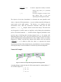
1 INTRODUCTION
In response to the growing need for improving the design and performance of
roadway facilities as well as for implementing innovative ITS technologies, engineers
are now increasingly relying on sophisticated, high-fidelity microscopic traffic
simulators rather than conventional approaches. Recognizing simulation’s
effectiveness and improved realism, the Federal Highway Administration (FHWA)
recently introduced a mandate requiring comprehensive simulation analysis to be
conducted for all new Interstate Access Requests (IAR) prior to actual
implementation. In this regard, high-quality input data are essential for building
realistic and accurate simulation models; such data include the roadway geometry,
vehicle/driver characteristics, traffic volumes, composition, and others. Among these
data, traffic volumes are of major importance as they are the starting point for
generating traffic demands and developing traffic control scenarios, and serve as
essential inputs for model calibration. However, reliable traffic volume data more
often than not are hard to obtain; even when collected with advanced surveillance
systems they are still susceptible to problems such as miscounting, gaps in time and
space and other inaccuracies caused by malfunctioning sensors. More importantly,
even though the data may appear to be accurate, frequently they do not balance out,
i.e., they are inconsistent in terms of maintaining traffic conservation throughout the
system, resulting in inaccurate traffic demands, unrealistic control decisions, and
erroneous adjustments of model parameters during calibration. Inevitably, these
problems could lead to anomalies or considerable errors during the simulation,
seriously tainting the reliability and accuracy of its outputs while weakening the
credibility of resulting conclusions.
Specifically, traffic volume data required in simulation include freeway volume data
and arterial intersection turning movements’ counts. For freeway volume data,
practical procedures and guidelines have been proposed in the literature for reviewing
and correcting common temporal errors [1-8]; however, most of them are not intended
for simulation purposes, while a unified systematic methodology is still lacking for
checking and correcting temporal data errors in conjunction with reconciling spatial
gaps in traffic counts. Likewise, frequently arterial intersection turning movement
counts are susceptible to errors of spatial gaps, yet there seems no well established
methodology existing in the literatures as to reconciling such gaps for simulation
purpose.
In this study, systematic methodologies have been proposed to check/correct common
temporal errors for freeway volumes. These methodologies also include rigorous
methods for reconciling both freeway volumes and arterial turning movement counts.
The proposed methodologies have been successfully automated and incorporated into
two computer programs called Freeway Traffic Data Analysis Tool (TradaX) and
1
Arterial Data Balance Tool (ArtBaT). Initial evaluations of these tools suggest that
they have the potential of reducing total modeling time by 25% ~ 30%, while
resulting in improved calibration of simulation models, more reliable analysis, and
better use of staff resources for meeting project deadlines.
2
2 BACKGROUND
The methodologies proposed in this study concentrate on improving the quality of
traffic volume data with the objective of enabling and improving traffic simulation.
This includes the integration of established procedures dealing with common temporal
errors with a new optimization-based algorithm reconciling spatial discrepancies. To
be sure, checking and correcting temporal volume errors, e.g., missing data, threshold
violations, or suspicious outliers, are not new and have been widely studied in
previous research [e.g., 9, 10, 11, 12, 13]. However, spatial discrepancies of traffic
volumes do not seem to have been adequately addressed; there is no guidance in the
literature on precisely what constitute a large discrepancy, nor does an effective
methodology seem to exist for checking and reconciling system-wide discrepancies
[14].
Existing procedures for checking temporal volume errors include tests for missing
data, threshold violation, locked-on sensors, data inconsistency, and temporal outliers.
Missing data refers to a situation where a detector fails to report any data within some
time duration. This is sometimes called data “holes” in the data set. Threshold
violation tests refer to the comparison of traffic measurements with prescribed upper
and lower bounds. For example, the lower/upper bounds for traffic volume used in
Maryland are based on historical data, while in Minnesota, a lower bound of 20 veh/5min per lane and an upper bound of 250 veh/5-min per lane are used [2]. Lock-on
sensors refer to situations where traffic measurements remain identical for several
consecutive data collection intervals. When this occurs, the values are in most cases
zero, but runs of values other than zero could also occur. Schmoye et al. [4] provided
an empirical method for determining the feasible run length (i.e., number of collection
intervals) of identical values. If the number of time intervals with identical values
became greater than a pre-determined run length, the data were considered to be
invalid. Another type of data error occurs when traffic volume and occupancy
measurements contradict each other, e.g., zero volume with non-zero occupancy, or
zero occupancy with non-zero volume. Payne and Thompson [3] identified this as
inconsistent data and proposed a test for its detection.
Temporal outliers refer to suspicious observations in the time series of traffic
measurements. Usually they are in the form of abrupt increases or decreases
inconsistent with the general pattern. Neural Network models, Genetic Algorithms
and Autoregressive Integrated Moving Average models (ARIMA) have been applied
to the outlier detection problem, mostly in other engineering domains. In the context
of traffic, a Fourier-based framework has been recently developed to detect outliers in
real-time traffic measurements [5] for the purpose of on-line control. In addition, a
fuzzy-clustering approach was also applied in identifying and correcting outliers in
archived traffic data [6].
3
Once faulty data are identified, they are excluded from the data set, or corrected either
empirically or using statistical methods. For example, Payne and Thompson [3] used
historical traffic information and the data from adjacent detectors to replace data holes,
while Turner et al [11] used regression and time series models, Chen et al. [12] used
lane-to-lane and location-to-location correlations to impute missing data. In addition,
if the faulty measurement was determined to be a temporal outlier, its modelpredicted [5] or smoothed value [6] was used as a replacement.
Apart from the aforementioned errors, frequently traffic volumes do not balance out,
i.e., they are inconsistent in terms of maintaining traffic conservation throughout the
system. In such cases, large discrepancies exist between traffic counts upstream and
downstream of specific locations. These spatial discrepancies may result from any of
the aforementioned errors, storage or discharge of queuing vehicles on the freeway,
traffic sinks or sources not accounted for, using data collected on different days or
time intervals, or simply averaging over different days at each measurement station
without checking conservation. Discrepancies may also arise from the inconsistent
projection of the base year demands into future years. As mentioned earlier, spatial
discrepancies of traffic counts have not been well addressed in previous studies.
4
3 CHECKING AND CORRECTING METHODOLOGY
This section presents the checking and correcting methodology implemented in
TradaX.
3.1 UNIFIED TRAFFIC DATA FORMAT
The Minnesota Department of Transportation (Mn/DOT) has one of the largest traffic
data collection systems in the United States. This system consists of more than 4000
loop detectors collecting traffic volume (number of vehicles), and occupancy
(percentage of time a detector is “occupied” by a passing vehicle) data in real time
every 30 seconds.
As the benefits of storing this large amount of data in a traditional database are far
offset by the accompanied complications, Mn/DOT finally turned to a Unified Traffic
Data File Format (UTDFF) . In this format, raw traffic data is stored as 8-bit (volume
data) or 16-bit binary numbers (occupancy data). This simple and compact format
greatly facilitates everyday data storage/retrieval, as well as development of data
analysis tools such as TradaX.
In UTDFF data format, each detector has two data files associated with it, i.e. volume
file (*.v30) and occupancy file (*.c30). The volume file (*.v30) is a flat binary file
with 2880 bytes in length. Each byte is an 8-bit signed integer corresponding to a 30second vehicle count. Within each volume file, the integer value of the first byte
represents the first 30-second vehicle counts of the day (i.e., from midnight to
12:00:30 am), while the last value corresponds to the final 30-second vehicle counts
of that day (i.e., from 11:59:30 to midnight). A negative value (0xFF) indicates
missing data (this 0xFF is generated by hardware controller if it receives no data from
detector).
The occupancy file (*.o30) is akin to volume files, except that each value is a 16-bit
signed integer. This means each file is 5760 bytes in length. As with the volume file,
a negative value (0xFFFF) indicates missing data.
In the end, all the detectors’ volume and occupancy files are zipped into one single
file on a daily basis. This single file is conventionally named with an 8-digit date
followed by an extension of “.traffic”. For example, “20031105.traffic” would contain
all the detectors’ volume and occupancy data of Nov 5th, 2003.
5
3.2 CLASSIFICATION OF DATA ERRORS
TradaX identifies and corrects data errors from two categories: common temporal
errors and spatial discrepancies.
(1). Common temporal errors refer to missing data, locked on sensors, contradictory
data, threshold violations, and temporal outliers. Such errors are called temporal
because they are associated with the time series of the measurements at each
individual detector.
(2). Missing Data refers to situation where a detector fails to report any data within
some time duration. This is sometimes called data “holes” in the data set.
(3). Lock-on Sensors means traffic measurements (both volume and occupancy)
remain identical values for several consecutive data collection intervals. When
this occurs, the values were most often zero, but cases of values other than zero
also are also frequent. When the identical value is zero, TradaX considers such
situation the same as data missing.
(4). Contradictory Data refers to the situation where traffic volume and occupancy
measurements contradict each other, e.g., zero volume with non-zero occupancy,
or zero occupancy with non-zero volume. TradaX considers contradictory data the
same as missing data (volume or occupancy missing).
(5). Threshold Violation means the collected traffic measurements exceed reasonable
upper and lower bounds. For example, 300 veh/5 minutes/lane is an out-of-bound
value as it entails an average flow rate of 1 veh/sec for the entire 5-minute period.
Different thresholds can be prescribed in practice to test the data. In Maryland, the
lower/upper bounds for traffic volume are based on historical data, while in
Minnesota, a lower bound of 20 veh/5-min per lane and an upper bound of 250
veh/5-min per lane are used.
(6). Temporal outliers refer to suspicious observations in the time series of traffic
measurements. Usually they are in the form of abrupt increases or decreases
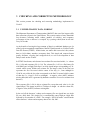
inconsistent with the general pattern (See Figure 3.1).
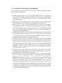
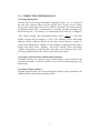
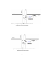
(7). Spatial Discrepancies refers to the situation where traffic volumes do not balance
out, i.e., they are inconsistent in terms of maintaining traffic conservation
throughout the system (See Figure 3.2). In such cases, large gaps exist between
traffic counts upstream and downstream of specific locations. These spatial
discrepancies may result from any of the aforementioned errors, storage or
discharge of queuing vehicles on the freeway, traffic sinks or sources not
accounted for, using data collected on different days or time intervals, or simply
averaging over different days at each measurement station without checking
conservation. Discrepancies may also arise from the inconsistent projection of the
base year demands into future years.
6
Figure 3.1 Traffic Volume Temporal Outliers (Three temporal outliers are indicated by arrows)
Figure 3.2 Spatial Discrepancies
For spatially correlated traffic detector stations, total input volume should approximate total output volume during a
given time period. As is shown In Figure 3.2, M1, M2, M3 are three mainline detector stations, E1 and E2 are two
entrance detector stations. If traffic volumes are balanced, vehicle counts at (M1+E1) should approximately equal to
those at M2.
7
3.3 CHECKING METHODOLOGY
Partial Missing Rate
As introduced earlier, raw volume and occupancy are collected on a 30-second basis.
These raw data are stored as 8-bit (volume data) or 16-bit binary numbers (occupancy
data). If during a 30-second interval, the hardware controller receives no data from the
detector, binary number 0xFF (8-bit binary representation of -1) or 0xFFFF (16-bit
binary representation of -1) will be used to indicate data “holes” for volume or
occupancy respectively.
It is required in many practical projects that raw 30-sec data (volume or occupancy, or
both) be aggregated into longer time interval such as 5 minutes or 15 minutes. This
leads to the concept of “Partial Missing Rate” (PMR). Specifically, PMR is defined
as the time percentage of the entire aggregation interval during which the
measurement is missing. The next example best illustrates this concept.
Assuming that raw 30-sec volume data are being aggregated into a 5-minute volume,
i.e., 10 successive 30-sec volumes are added up to yield a 5-minute volume. If four
out of the ten 30-sec volume data are missing (i.e., they are flagged as “-1” by the
controller), the Partial Missing Rate for the aggregated 5-minute volume will be 40%
(4 divided by 10). Note that TradaX computes the Partial Missing Rate for any
aggregated time interval greater than 30-sec.
Checking Missing Data
TradaX filters missing data by first checking the Partial Missing Rate (PMR). If the
PMR of an aggregated volume (or occupancy) is non-zero, TradaX will flag such data
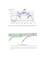
as missing and report related information in the data scanning log (Figure 3.3). As
Figure 3.3 shows, Detector 1351 (which belongs to Station 426) at 19:00 have 3%
volume missing, meaning from 18:55 to 19:00, three of the ten 30-sec raw volume
data are missing.
8
Figure 3.3 Scanning Log Showing Partial Missing Rate for Detectors/Stations
Apart from the hardware reported data missing, TradaX also applies the following
heuristic rules to supplement the determination of missing data. Note if any of the
following rules are found to hold, the related measurement will be flagged as 100%
missing and reported in the scanning log accordingly:
1. Zero Volume with non-zero occupancy ( 100 % volume missing );
2. Zero Occupancy with non-zero volume ( 100% occupancy missing );
3. Non-HOV detectors report zero volume and zero occupancy for 2 consecutive
aggregated time intervals (100 % volume missing and 100% occupancy
missing);
Note that HOV detectors are not included in Rule 3, as it is highly probable for HOV
detectors to have zero measurements during multiple data collecting periods. Further,
it should be stressed that Rule 3 is very likely to generate a false alarm during nonpeak periods, e.g., from midnight to 4:00 a.m. in the morning. In this case, the user is
strongly suggested to examine the Data Scanning Log and visually check/verify the
reported missing data (during non-peak hours) using the Data Graphics function.
Figure 3.4 gives the flow chart for filtering missing data.
Filtering Locked-on Sensors and Threshold Violations
TradaX considers the data as locked on if both volume and occupancy have non-zero
values and remain identical (unchanged) for two consecutive data aggregation
intervals. Furthermore, if the data exceed user-defined threshold values TradaX will
flag the data as violating thresholds.
9
Figure 3.4 Filtering Missing Data Flow Chart
10
Filtering Temporal Outliers
In order to filter temporal outliers, the ARIMA (p,d,q) model was selected in this
study and fitted using field data to determine the best parameters. Specifically, the
ARIMA (p, d, q) model can be represented as:
X t = ξ + φ1 X t −1 + φ2 X t − 2 + ... + φ p X t − p − θ1ε t −1 − θ 2ε t − 2 − ... − θ q ε t − q + ε t
(1)
where
ξ
Xt
is a constant;
represents the observation at time t;
φ n is the autoregressive parameter, n = 1,2,..., p;
θn
is the moving average parameter, n = 1,2,..., q;
εt
is white noise random error at time t, ε t ~ WN (0, σ 2 ) ;
p is the number of autoregressive terms;
q is the number of moving average terms;
d is the order of differencing needed to make the time series stationary.
It should be noted that the ARIMA model only applies to stationary time series (i.e.,
for time series { X t }, the mean value E( X t ) is constant and the covariance E( X t
X t−h
)
is only dependent on the time lag h ). In this study, the ARIMA model represented by
equation (1) was fitted to historical traffic counts and occupancy time series to
determine the appropriate p, d, and q values. The historical data were measured at 10
randomly selected detectors from the Twin Cities freeway network. Note that traffic
counts and occupancy measurements are non-stationary as they clearly have timedependent tendencies. In order to produce stationary time series from these
measurements, the square root was calculated followed by differencing until
stationary time series were obtained. After some experimentation, the ARIMA (1, 1, 1)
model was found to be most appropriate for modeling the square root of the traffic
count and occupancy time series for all the detectors.
The fitted ARIMA model produces a prediction of the likely actual measurements at
each time interval based on the preceding measurements. At any time interval, the
difference between the predicted value and actual observation produces a residual. A
measurement is labeled as outlier if the standardized residual exceeds a specified
confidence level. For instance, any standardized residual value greater than 1.96
would indicate a highly probable temporal outlier with 95% confidence level. Figure
3.5 illustrates an example of traffic sensor volume measurements (loop detector
No.982 on I-94, August 3 rd, 2000). In this figure, three suspicious outliers are
indicated by the arrows. Figure 3.4 also includes the z-statistics of the residuals after
the fitted ARIMA model has been applied. It is clearly depicted in the figure that the
11
three suspicious outliers correspond to high z-statistics exceeding the critical residual
value.
Figure 3.5 (a) Traffic Volume Outliers
Figure 3.5 (b) Z-Statistics for Traffic Volumes
12
3.4 CORRECTING METHODOLOGY
Correcting Missing Data
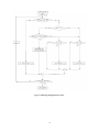
The flow chart for correcting missing data is depicted in Figure 3.6. As is shown in
the flow chart, detectors that have been flagged with a specific Partial Volume
Missing Rate smaller than 100% will be fixed by “rescaling.” This means that true
measurement values will be reconstructed by “rescaling” raw data according to the
partial missing rate. For example, if a measurement of 50 veh/5-min is flagged as
“40% volume missing,” the reconstructed volume will be
50
= 83
1 − 40%
veh/5-min.
Further, detectors that are flagged as “100 % VOL Missing” will be fixed using
adjusted “sibling” (adjacent detectors in the same station) detector’s volume, or
conservation computation if “siblings” are not available, or applying historical data if
neither of the above works. Similarly, “100 % OCC missing” will be fixed using
“sibling” measurement or historical data. Note that in case historical data is also
missing, predefined default value will be used to fill the data “holes.”
Correcting Locked on Sensors and Threshold Violations
Threshold violations are corrected using prescribed upper or lower bounds for the
related measurements. Locked-on sensors are corrected in the balancing stage to be
detailed next.
Correcting Temporal Outliers
Detected temporal outliers are corrected using the predicted value generated by the
ARIMA model as discussed in preceding sections.
13
Start Correcting
Missing Data
Set j = 0
Is Sensor j
flagged as have
missing data?
NO
YES
Vol Missing?
NO
YES
NO
Is partial Missing rate
100%?
Is partial Missing rate
100%?
YES
YES
j= j+1
NO
Is sensor j’s sibling
flagged
as “Vol Missing’ ?
YES
YES
Can Sensor j be fixed by
conservation?
NO
Is sensor ‘s sibling flagged
as “Occ Missing”?
YES
NO
NO
Historical Data
Available?
YES
Fix Sensor j by
“recaling”
Multiply sibling’s
vol by a
predefined
adjustment
factor. Use the
adjusted vol as
sensor j’s
volume
Fix Sensor j using
conservation
principle
Fix Sensor j using
predefined default
values
NO
Fix Sensor j using
historical data
Is sensor j the last
sensor?
Stop Filtering
Missing Data
Figure 3.6. Flow Chart for Correcting Missing Data
14
Use sibling’s occ as a
substitute for sensor j’s
occ
NO
4 RECONCILING METHODOLOGY
4.1 IDENTIFICATION OF SPATIAL DISCREPANCIES
Once the temporal errors have been processed throughout the dataset, jumps or drops
of traffic counts at all nearby adjacent mainline counting stations are checked in
sequential order (i.e., from upstream to downstream). Specifically, for every freeway
section between two successive mainline counting stations, the difference between
total input (i.e., total traffic counts at the upstream counting station and entrance
ramps) and output volumes (i.e., total counts at the downstream counting station and
exit ramps) is computed for every data collection interval. If the discrepancy (denoted
as ∆C ) exceeds a reasonable threshold, then this discrepancy is considered large
enough and needs to be reconciled.
In order to determine the allowable discrepancy threshold ∆C , the concept of traffic
conservation is considered:
t+∆t
[ ∫ q ( x u , t ) dt + ∑
t
e∈ E
xd
x
d
xu
x
u
= ∫ k ( x, t + ∆t )dx - ∫
t + ∆t
t + ∆t
t
t
∫ q ( x e , t ) dt ] - [ ∫ q ( x d , t ) dt + ∑
t + ∆t
ex ∈ X
∫ q ( x ex , t ) dt ]
t
(2)
k ( x , t ) dx
where ∆t is the data collection interval (e.g., 5 min or 15 min); E is the index set for
counting stations at entrance ramps; X is the index set for counting stations at exit
ramps; q ( x u , t ) , q ( x d , t ) , q ( x e , t ) , q ( x ex , t ) are the flow rate at upstream, downstream,
entrance ramp and exit ramp counting stations, respectively; k ( x, t ) is traffic density of
the freeway section delimited by upstream and downstream counting stations. The
left-hand side of Equation (2) is equivalent to the difference between total input and
output during interval ∆t , which equals ∆C ; the right-hand side of Equation (2) can be
approximated from
[ k ( x, t + ∆t ) − k ( x, t )].( x d − x u ) = [k ( x, t + ∆t ) − k ( x, t )].∆x
(2a)
where ∆x is the distance between upstream and downstream counting stations. Using
the relationship between occupancy measurement and traffic density:
K≈
O
L+C
(3)
where O is occupancy measurement, K is density, L is average vehicle length, C is
the detector length, Equation (4) can be simplified to:
∆C ≈ [ K (t + ∆t ) − K (t )] × ∆x
(4)
15
where K (t ) and K (t + ∆t ) are traffic densities approximated from Equation (3).
Equation (4) gives the allowable upper bound for the discrepancies of traffic counts,
i.e., if the computed discrepancy exceeds the bounds defined by | [ K (t + ∆t ) − K (t )] × ∆x |,
then such a discrepancy is considered to violate traffic conservation therefore needs to
be reconciled. However, it is important to clarify that if the counting interval is
sufficiently long, or the analyst is only interested in homogeneous state of traffic,
where traffic density is assumed to be uniform (i.e., time and space invariant), then
∆C ≈ 0, meaning that the total input should always equal to the total output of the
freeway section. NOTE: In the current version of TradaX, ∆C is hard-coded as 0,
meaning TradaX always balance traffic volume to zero.
4.2 RECONCILING SPATIAL DISCREPANCIES
The identified large discrepancies in traffic counts are reconciled in this step. First
denote the number of the counting stations under study (including stations on
mainline, entrance and exit ramps) as N sta . At counting interval t, for the counting
station i let y i (t ) denote raw field measurement of traffic counts, xi (t ) denote the true
measurement of traffic counts, and ε i (t ) the measurement error. Then y i (t ) can be
expressed as
y i (t )
= xi (t ) + ε i (t ) , i = 1, 2… N sta
(5)
The measurement errors ε i (t ) in Equation (5) may be in relation to errors discussed in
preceding sections, inconsistent adjustments between different days, of or small
random miscounting errors due to unknown reasons.
Note that counting stations are deployed in certain spatial arrangement; this triggers
conservation constraints, i.e., for spatially related counting stations on a given
freeway section, the difference between input and output equals the change of vehicle
storage during the specified counting interval. In order to reconcile large
discrepancies in traffic counts while at the same time minimize the measurement
errors, the following optimization formulation is used:
minimize ∑ ε i (t ) = ∑ [ y i (t ) − xi (t )] 2 , ∀t
i
i
s.t.
Conservation Constraints as In Equation (2)
xi (t ) ≥ 0 , i = 1,2,..., N sta
16
(6)
|
x i (t ) − y i (t )
| < p% ,
y i (t )
for station i diagnosed as “healthy” in the data
filtering stage, where p% is prescribed
parameter;
for station i flagged as erroneous in the
xi < ∞ ,
data filtering stage, or has been
adjusted/projected using historical data;
The objective of the above formulation is to determine the most plausible actual
values xi when the field measurements y i are given without materially affecting the
actual trends in the traffic patterns. The objective is to minimize the total
measurement errors, while the conservation constraints ensure that the final
optimizer xi , i = 1,2,..., N sta complies with the conservation concept. This means that
any discrepancies in traffic counts are implicitly resolved during this optimization
process. The relaxed constraint xi < ∞ holds for station i flagged as problematic in the
previous stage of checking and correcting temporal errors, or for stations with
adjusted/projected counts. This is necessary otherwise the errors associated with a
specific counting station will be distributed over other “healthy” stations. As stations
diagnosed as “healthy” could still have inherent small random errors, the constraint
|
x i (t ) − y i (t )
y i (t )
| < p % is added to reflect this, where p % represents the desired
measurement precision of the related detectors, stated otherwise it is also an indicator
reflecting the analyst’s desired confidence level based on professional judgments.
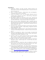
Numerical Example
Figure 4.1 Numerical example illustrating the data balancing algorithm
Assuming during a certain time interval, field measurements for counting Station1~ 7
are as follows (Figure 4.1):
y1 = 20
veh
y 2 = 20
veh
y 3 = 170 veh
17
∆ storage1 = 10 veh
y 4 = 30
veh
y 5 = 95
veh
∆ storage2 = 15 veh
y 6 = 40
veh
y 7 = 40 veh
∆ storage3 = 10 veh
Furthermore, assuming Station 3 and Station 7 are flagged as “threshold violations”
and “temporal outlier” respectively. Thus we have the following optimization
problem:
min ( x1 -20) 2 + ( x 2 -20) 2 + ( x 3 -170) 2 + ( x 4 -30) 2 + ( x 5 -95) 2 + ( x 6 -40) 2 + ( x 7 -40) 2
Subject to
Conservation Constraints:
 x1 + x 2 − x 3 = 10

 x 3 + x 4 − x 5 = −15
 x − x − x = −10
6
7
 5
Non-negative Constraints: xi ≥ 0 , for i = 1,2,...,7
Precision Constraints: |
x i (t ) − y i (t )
|
y i (t )
< 3%, for i ≠ 3, i ≠ 7
Relaxed Constraints: x 3 < ∞ ; x 7 < ∞ ;
Solving the above optimization problem yields the optimized solutions:
( x1 , x 2 , x 3 , x 4 , x5 , x 6 , x 7 ) = (22, 22, 54, 28, 97, 44, 63)
18
5 ARTERIAL BALANCING METHODOLOGY
This section describes the underlying methodology employed in the ArtBaT program.
Specifically, this methodology involves three stages: data normalization, data
matching, and data balancing.
5.1 DATA NORMALIZAION
Intersection volume data sets are collections of 15-minute volume for individual
turning movement (e.g., 50 left-turn vehicles, 100 right-turn vehicles, 276 through
vehicles, etc) collected over a 3 hour time period. As the number of intersections
requiring turning movement counts usually exceeds the available manpower, turning
movements are seldom collected on the same day or even the same month. Therefore,
turning movements should be first normalized (adjusted) to match the month and day
of the balanced freeway data, should monthly/daily adjustment factors be available.
To normalize arterial turning movement data, the following formula is used:
Vol 2 =
Vol1 × M 1 × D1
M 2 × D2
(7)
where
Vol1 : Raw
arterial volume.
Vol 2 : Normalized
M1
arterial volume.
: Monthly adjustment factor for the month when the arterial data was
collected.
M 2 : Monthly adjustment
D1 : Daily adjustment
D2 :
factor for the month of the balanced freeway data.
factor for the day when the arterial data was collected.
Daily adjustment factor for the day of the balanced freeway data.
19
Data Normalization Example
Assume that on a Wednesday in May, 100 thru vehicles were counted
at a certain intersection approach; while the balanced freeway data
are given for a Tuesday in September. In addition, the adjustment
factors are given as:
ü Monthly adjustment factors: May 0.95, September 0.85;
ü Daily adjustment factors: Wednesday 1.10, Tuesday 1.15.
In order to match the date of the freeway data, the normalized arterial
data are computed as:
100 × 0.95 × 1.10
Vol 2 =
= 107
0.85 × 1.15
5.2 DATA MATCHING
The balanced arterial data must match the balanced freeway ramp volume. This is
achieved by using the raw turning movement volume to determine the percentage of
left-turn, right-turn, and thru movements on ramp intersection legs. These percentages
are applied to the balanced freeway ramp data to get the new volumes which are then
locked when balancing the remaining arterial volumes.
Data Matching Example
Assume that the collected arterial data includes 35 left-turn and 87 rightturn vehicles for a ramp leg (Figure 5.1(a)). This gives the percentage of
35
87
left turn vehicles as
= 28.6% and right turn vehicles as
=
35 + 87
35 + 87
71.4%. However, the freeway ramp volume is reported to be 135 vehicles
(as a result of freeway balancing). Therefore, the matched new arterial
volumes for this leg are 135 × 28.6% = 39 left-turn vehicles and
135 × 71.4% = 96 right-turn vehicles. These movements are then locked
while balancing the remaining arterial data (Figure 5.1 (b)).
20
Figure 5.1 (a). Example illustrating how to match arterial intersection data
to balanced freeway data (before matching).
Figure 5.1 (b). Example illustrating how to match arterial intersection data to
balanced freeway data (after matching).
21
5.3 DATA BALANCING
In a nutshell, balancing arterial intersection turning movement data means adjusting
the relevant turning movement volumes so that the total traffic entering a link equals
the total traffic exiting the link. This is conducted by proportioning the extra link
volume (i.e., the volume difference between the total inflow and total outflow of a
link) among any movements that can be changed. Specifically, the formula used in
this process is:


V ij = V ij ± ∆ V 





V ij 

V ij
∑
where:
Vij
= the balanced volume of movement j in direction i ;
Vij
= the raw volume data for movement j in direction i;
∆V
= the volume differential between turning count data sets for a specific link.
22
(8)
REFERENCES
1.
2.
3.
4.
5.
6.
7.
8.
9.
10.
11.
12.
13.
14.
Jacobson,L.N., Nihan,N.L. and ender J.D.(1990), “Detecting Erroneous Loop
Detector Data in a Freeway Traffic Management System,” Transportation Research
Record, 1287, pp151-166
Chen L., and May A.D.,(1987), “Traffic Detector Errors and Diagnostics,”
Transportation Research Record, 1132, pp82-93
Payne,H.J. and Thompson, S.(1997), “The I-880 Database: Malfunction Detection
and Data Repair for Induction Loop Sensors,” Annual Meeting, Transportation
Research Board, Washington D.C.,1997
Rick Schmoyer, Patricia S. Hu, and Richard T.Goeltz (2001), “Statistical Data
Filtering and Aggregation to Hour Totals of Intelligent Transportation System 30s
and 5-min Vehicle Counts,” Transportation Research Record, 1789, pp79-86.
Srinvas Peeta and Ioannis Anastassopoulos (2002), “Automated Real-Time
Detecting and Correction of Erroneous Detector Data Using Fourier Transforms for
On-line Traffic Control Architectures,” Annual Meeting, Transportation Research
Board, Washington D.C. 2002.
Sherif Ishak (2003), “Quantifying Uncertainties of Freeway Detector Observations
Using Fuzzy-Clustering Approach,” Annual Meeting, Transportation Research
Board, Washington D.C., 2003.
Cleghorn D., Hall F.L. and Garbuio D.(1991), “Improved Data Screening Technique
for Freeway Traffic Management Systems,” Transportation Research Record,1320,
pp17-13
Turochy, R.E. and Smith B.L. (2000) “A New Procedure for Detector Data
Screening in Traffic Management Systems,” Paper No. 00-0842, Annual Meeting,
Transportation Research Board, Washington D.C, 2000.
Nguyen,L.N., Scherer, W.T. (2003) “Imputation Techniques to Account for Missing
Data in Support of Intelligent Transportation Systems Applications,” Research
Report No. UVACTS-13-0-78, May 2003, University of Virginia
Conklin, J.H., Scherer, W.T. (2003) “Data Imputation Strategies for Transportation
Management Systems,” Research Report No. UVACTS-13-0-80, May 2003,
University of Virginia
Turner, S.M., Eisele, W.L., Gajewski, B.J., Albert, L.P. and Benz, R.J. (1999) “ITS
Data Archiving: Case Study Analysis of San Antonio TransGuide Data,” Report
No.FHWA-PL-99-024, Aug 1999, Texas Transportation Institute
Chen,C.,Kwon,J.,Rice,Jl,Skabardonis,A. and Varaiya,P.(2002) “Detecting Errors
and Imputing Missing Data for Single Loop Surveillance Systems,” paper presented
at 82nd Annual Meeting, Transportation Research Board, Jan,2003,Washington,D.C.
Bickel, P., Chen, C., Kwon, J., Rice, J., Zwet, E. and Varaiya, P. (2004) “Measuring
Traffic,” http:// www.stat.berkeley.edu/users/rice/664.pdf, accessed at Oct 15, 2005
FHWA (2004) “Traffic Analysis Tool Box Volume III: Guidelines for Applying
Traffic Microsimulation Modeling Software,” Report No. FHWA-HRT-04-040
23
Appendix A
Freeway Traffic Data Filtering and Balancing Tool
TradaX Version 2.0
User Manual
SOFTWARE OVERVIEW
INTRODUCTION
TradaX (Traffic Data Analysis) is a Windows© software package designed and
developed at the University of Minnesota for filtering, correcting and balancing
freeway traffic data. It can automatically identify freeway geometry and retrieve
traffic data in UTDFF format, filter and correct data faults, and reconcile spatial
discrepancies of traffic volumes. It also provides rich graphical functionalities and
flexible data output options to facilitate data examination and outputs.
TradaX integrates empirical procedures, in conjunction with a validated ARIMA
(Auto-Regressive Integrated Moving Average) model to filter and correct common
temporal data errors; while a non-linear optimization algorithm has been developed
and implemented in TradaX to balance the identified gaps of traffic counts on a
system-scale.
INSTALLATION
System Recommendations
CPU
Memory
Operating Systems
Resolution
> 1GHz
256MB ( 512 MB Preferable)
Windows ME/NT/2000/XP
1280 × 960 Preferable
Installation Directions
The installation package includes user manuals, samples and executable program.
Two types of installation are available:
Beta Version
1. Select a working directory and unzip TradaX.zip file (Windows Registry will
not be modified);
2. Double click TradaX.exe to start the program;
3. To uninstall, delete all the files in the working directory;
Release Version
1. Before installing, it is suggested to close any running Windows programs;
2. To install new TradaX, click setup.exe and follow the screen instructions;
3. To uninstall, from START menu, under TradaX directory click UNINSTALL,
the uninstall program will automatically remove the software from the
computer.
A-1
USER INTERFACE
TRADAX INTRODUCTION PAGE
Figure A.1 Tradax Introduction Page
When starting TradaX.exe, TradaX introductory page will first show up. This page
provides general information of the program, including built date and system
resources information.
TREE VIEW OF ACTION LISTS
Figure A.2 Tree View of Actions List
TradaX organizes its functionalities via a tree view list (located in the left part of the
interface). The tree view has three father nodes: Data Processing, Data Graphics, and
Help, corresponding to three major functionalities provided by TradaX.
A-2
Data Processing includes:
• Data Extraction
• Data Fix
• Data Balance;
Data Graphics can generate graphics for Raw Data, Fixed Data and Balanced Data
while Help provides on-line help for the user.
TIPS The user can use either the Tree View List or the “Previous”/”Next” button to
navigate through user interfaces.
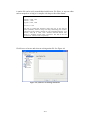
EXTRACT BINARY TRAFFIC DATA
Figure A.3 Extract Binary Traffic Data General Information Page
Prior to fixing and balancing, traffic data must be loaded (extracted) into TradaX
memory. Figure A.3 shows the general information page of Extract Data functionality.
The user can click the link on the page, the action node in the tree view, or Next
button to proceed.
Load Station File
Before starting to extract data, a station file needs to be loaded. Station files are
ASCII files with .sta extension. It provides a convenient way describing the spatial
layout of detector stations that are deployed on the freeway.
A-3
A station file can be easily created/edited with Station File Editor, or any text editor
such as notepad.exe as long as it complies with the prescribed data format.
An example of a station file:
…….
426, M, 2, 1350, 1351
1352 X, 1, 1352
427, M, 2, 1353, 1354
……..
1919, H, 1, 1919
Each line in station file describes name and type of the detector
station (mainline, entrance ramp, exit ramp, HOV ramp), the number
of detectors in the station, and IDs of each composing detector. For
instance, “426, M, 2, 1350, 1351” describes detector Station 426,
which is a mainline station with 2 detectors. The IDs of the two
detectors are 1350 and 1351 respectively.
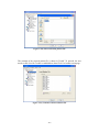
Click Browse to browse and select an existing station file. See Figure A.4
Figure A.4 (a) Browse an Existing Station File
A-4
Figure A.4 (b) Select an Existing Station File
The contents of the selected station file is shown in TradaX. To proceed, the user
needs to click Load for TradaX to establish data; then Click Next button to next page.
Figure A.4 (c) Contents of Selected Station File
A-5
Load and Extract Binary Data
Browse and Load Binary Traffic File
Once the station file has been loaded, TradaX needs to know about the location of the
binary traffic data file. Use Location button to navigate and select the required binary
file.
Extraction Options
Time Interval
After select appropriate binary file, the data aggregation interval should be designated
(the default value is 15 minutes, i.e., Tradax will aggregates 30-sec raw data into 15min interval data).
Station Occupancy
TradaX extracts data in terms of individual detector as well as stations. Station
occupancy is derived either from averaging detector occupancies, or taking highest
detector occupancy.
Extract Button
Click Extract button to start extract data.
Save Options
The extracted (raw) data can be saved as .csv file either in terms of detectors or
stations. The data can be in row format or column format.
Figure A.5 Load and Extract Binary Traffic Data
A-6
An example of saved data in Row Format
An example of saved data in Column Format
A-7
FIX DATA
After data have been successfully extracted, click “Next” button to the Fix Data
general information page. This page provides general information about the “Scan for
Data Errors” and “Fix Errors” functionality. Click “Next”, or select Scan for Data
Errors, to proceed.
Figure A.6 Fix Data General Information Page
Scan for Data Errors
TradaX scans the loaded data for errors. The user needs to specify volume and
occupancy thresholds and the scanning log option in this page. Then click Scan Data
button to start scanning.
Figure A.7 Scan for Data Errors Page
A-8
Threshold Setup
The default volume and occupancy thresholds are 900 veh/15min, and 99/15min, respectively.
The user can setup different threshold values through the edit box.
Outlier Detection Model
In current version of TradaX, a fitted ARIMA model is implemented to detect temporal
outliers.
Scan Log Options
When data scanning is completed, a log that lists detected errors will pop up (See
Figure A.8). The user can customize the log output by specifying which type of error
he wishes to scan for via Scan Log Options.
The scan log can be saved as .csv file (A csv file can be opened with Microsoft Excel
or any text editor such as notepad.exe) for later reference.
Figure A.8 Scanning Log Listing Detected Errors
A-9
Fix Data Page
Lane Adjustment Factor
Input Lane Adjustment Factor for different lanes (default value is 1.00), where L0 is
the rightmost lane, L1 is the second rightmost lane, etc. Lane Adjustment Factor will
be used when fixing missing data with adjacent detectors.
For example, if L0 volume is missing, L1 volume available, and L0 = 1.10 and L1 =
1.25; L1 has a volume of 100 veh/5min, then L0 is reconstructed by (100 × 1.25/1.10)
= 114 veh/5 min.
Figure A.9 Fix Data Page
Reference Dates for Missing Data
The two reference dates are for correcting missing data, i.e., when the missing data
can not be corrected by adjacent detector value, or using conservation computation,
historical data from these two dates, whichever is available, multiplied by the Daily
Adjustment Factor ( default value is 1.00 ) will be used as substitute for the missing
one.
Default Value
When the missing data can not be fixed by adjacent detector, conservation
computation, or historical data, the default volume value will be used to fill the data
holes.
A-10
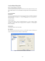
Advanced Options
By default, TradaX will fix 24-hour raw data for all the detectors listed in the station
file. However, the user may not desire a 24-hour fixing and may wish to fix the data
for a 2-hour period with only a few detectors. This can be accomplished via
Advanced Options. To setup desired time period for fixing and specify detectors to
be fixed, click Advanced button (See Figure A.10)
Figure A.10 Advanced Options for Fixing Data
Start Fixing
Click Fix button to start fixing the detected data errors. A Fixing Recommendations
Dialogue will pop up (See Figure A.11). The user needs to approve these
recommendations for TradaX to implement them (Click Select All button to approve
all at once, or check each individual recommendation one by one).
Click “Accept” to approve the checked recommendations.
A-11
Figure A.11 Fixing Recommendations
A-12
BALANCE DATA
Balance Data General Information Page
Figure A.12 Balance Data General Information Page
Balance Data ConFigure A.uration
Balance Interval
The user can designate the balancing interval. (e.g., the user may wish to balance data
from 3:00pm to 6:00pm) See Figure A.13
Figure A.13 Balancing Interval Setup
A-13
External Data File
The user can also designate Lock Station file and Flag Station File. If such files are
not needed, leave the input blank. See Figure A.14.
Figure A.14 External Data Files Setup
Lock Station File
By “lock”, it is meant that the data in this file is considered to be error-free; hence in
the subsequent balancing process, these data will be left untouched, while other “nonlocked” station will be modified whenever necessary by the algorithm to achieve
balanced results.
The data in the Lock Station File could be results from other freeway balancing. For
example, the “locked” station could be one of the boundary stations that are shared by
two freeways. If the data of such station have already been balanced for one freeway,
then the user may wish to lock this station when proceed to balance the other. “Lock
Station” is useful especially when the user intends to balance loop detector station
data on a network-wide basis.
Lock Station File should be strictly in the following format:
A-14
NOTE:
1. The file may have more data lines depending on the number of locked stations.
2. Comment lines are not parsed by the program.
3. The Data Line MUST be comma separated. NO TAB are allowed in the file (Be
cautious! The program is VERY sensitive when parsing the Load Station File. )
4. It is stressed in the strongest term that ONLY Boundary stations (i.e., upstream
freeway entrance station and ramp entrance/exit stations) can be lock stations. The
program can still generate outputs when non-boundary stations (e.g., mainline
stations) are locked, but the user should be warned that the results are not reliable.
5. It is VERY important that the number of data items in the data line match the
number of time stamps determined by start time and end time. For example, start
time 14:00 and end time 15:00 with 15 minutes time intervals, would give 5 time
stamps, i.e., 14:00,14:15,14:30,14:45,15:00. If the data line includes 6 data items, e.g.,
300,350,325,340,332,360, then this data line is inconsistent with the time stamps.
This situation should be strictly avoided.
Flag Station File
This function is added because during the data fixing stage, certain data errors can not
be properly filtered and corrected, for example, the kind of errors illustrated in the
following Figure A.15 This kind of errors is unusual and can only be discovered
through visual checking. However, errors like this have to be corrected in order to
ensure the credibility of balancing results.
The data in the Flag Station File will be used to replace the recommended fixing
proposed by the program when the user determines the latter is not reliable. Note the
TradaX program will modify the Flag Station data whenever necessary to achieve
balanced results.
Flag Station File must comply with the following format:
A-15
The file may have more data lines depending on the number of flagged stations.
Comment lines are not parsed by the program. The Data Line MUST be comma
separated.
Figure A.15 An unusual data error that can not be properly filtered
A-16
Warning Setup
The user can active the Warning Message Setup for balancing. This means a warning
message will be generated if the zone balance (i.e., the difference between total input
volume and output volume of a zone) exceed the user-defined threshold. See Figure
A.16
Figure A.16 Balancing Warning Setup
Start Balance
Click Balance button to start balancing. A Balance Log will pop up when the program
completes balancing. See Figure A.17
Figure A.17 Balancing Log
A-17
ZoneID
The “ZoneID” is a combination of upstream and downstream station IDs for the
freeway section has these two stations as endpoints.
I/O difference_1
This is the difference of total input volume and output volume before the balancing.
I/O difference_2
This is the difference after balancing. TradaX always balances I/O difference_2 to
zero. A warning message will be put to NOTE if I/O difference_1 exceeds the userdefined threshold.
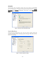
Balance Outputs
The user can specify the output format for the balanced data. See Figure A.18. Note
Output Time Interval is the same as the Balance Interval, which can only be modified
through “Balancing Configuration” page.
Figure A.18 Balance Outputs Setup
A-18
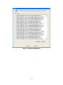
Example of Column Format (including Balanced/Fixed/Raw Volumes) :
Example of Row Format (includes Balanced Volumes only):
A-19
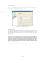
DATA GRAPHICS
Data Graphics General Information Page
Figure A.19 Data Graphics General Information Page
Data Graphics Plot Page
Select Station ID or Detector ID from the Tree View List, specify Time Interval, then
click Plot button.
Figure A.20 Data Graphics Plot Page
A-20
Data Plot
The data plot includes plots for Raw Data, Fixed Data, and Balanced Data. See Figure
A.21.
Figure A.21 TradaX Data Plot
ON-LINE HELP
The user can start on-line help (See Figure A.22) by click Start Help Engine on the
Help Content Page.
Figure A.22 TradaX On-Line Help
A-21
Appendix B
Arterial Intersection Data Balancing Tool
ArtBaT 1.0
User Manual
OVERVIEW
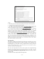
Figure B.1 gives a snapshot of the main interface of ArtBaT. As is shown in this
figure, ArtBaT interface has four major components:
(1) Geometry Type Library;
(2) Drawing Area;
(3) Draw Function Keys;
(4) Balancing Direction Selection Radio Button;
It is through these components that the user interacts with ArtBaT to balance arterial
intersection data.
Geometry Type Library
Geometry Type Library contains all the possible arterial intersection types that could
be encountered in practice. By clicking the geometry type icons, the user can build a
certain layout of several intersections. So far, ArtBaT program can handle up to 17
types of intersections.
Drawing Area
Drawing Area is where the user builds and configures intersection geometries. Up to
SIX intersections (of different types) can be balanced using ArtBaT program.
Draw Function Keys
•
Clear Draw : Clear the entire drawing area;
•
Undo Last
•
Refresh
: Delete the last intersection;
: Refresh the drawing area;
• Check Draw: Check the geometry configuration before run
“balancing data” command.
B-1
Balancing Direction Selection Radio Button
•
Select relevant radio button to designate the balancing direction.
Figure B.1 Snapshot of ArtBaT User Interface
B-2
MENU ITEMS
ArtBaT has six menu items: File, Data, Output, Run, Help and About.
File
Ø Load Scenario : Load existing balancing scenario ;
Ø Save Scenario : Save current configurations as scenario ( *.sco ) ;
Ø Exit : Exit the ArtBaT program
NOTE A scenario file consists of the following information
•
Number of intersections to be balanced;
•
Intersection types for each intersection;
•
Intersection Data Files;
Data
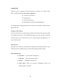
Ø Load Intersection Data File: This command loads intersection data
file.
NOTE:
Intersection Data File must comply with the following format (which is
the same format as JAMAR file, See Figure B.2)
(1). TXT file format (can be edited using notepad.exe)
(2). Line 1 to line 10, inherited format from JAMAR file format,
carrying no specific meaning to ArtBaT program;
(3). Line 11 to the last line: must be comma separated,
containing 1 time stamp column (i.e., the 1st column) and 16
data columns (i.e., 2nd to 17th columns)
(4). For those turning movements related to freeway
entering/exiting ramps, ArtBaT assumes the user has
already conducted necessary data matching/splitting (See
Section 2.2), i.e., the data file to be loaded by ArtBaT are the
already-matched data;
(5). The user is suggested in the strongest term to examine the
JAMAR data file prior to inputting required column numbers.
(6). Total number of data lines that ArtBaT can handle is 96 ( this
is based on the assumption that the data are on 15-min
basis and 24 hours contain ninety-four 15-min intervals)
B-3
Figure B.2 A Sample of Intersection Data File
Output
Ø Output Directory: Designate output directory for the balancing results.
NOTE:
•
•
Balancing results will be stored in the designated output directory
as *.csv files that can be opened with Excel;
One intersection will have two output files associated with it, i.e.,
intersection_name.csv, which contains integer-valued balanced
results, and intersection_name_float.csv, which contains
floating point valued balanced results. Here “intersection_name”
represents the name of the intersection in question.
Run
Ø Balance Data: this command will execute the data balancing
subroutine on the intersections.
NOTE: Run-> Balance Data command is disabled unless the
intersections pass geometry check (to perform geometry check, click
“Check Draw” button)
B-4
EXAMPLE
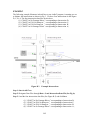
The following example illustrates in detail how to use ArtBaT program. Assuming we are
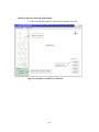
to balance the intersections as shown in Fig 3. We have four intersections in this figure:
D, C, B, A. The four intersection data files involved are:
(1) “CSAH73 at No Frontage Rd.txt ” corresponding to Intersection D;
(2) “CSAH73 at I394 No Ramp.txt ” corresponding to Intersection C;
(3) “CSAH73 at I394 So Ramp.txt ” corresponding to Intersection B;
(4) “CSAH73 at So Frontage Rd.txt” corresponding to Intersection A;
Figure B.3
Example Intersections
Step 1: Start ArtBaT.exe
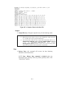
Step 2: Designate Data Files through Data → Load Intersection Data File (See Fig 4);
Step 3: Load the four intersection data files (See Figure B.5) and click Save
(1)
(2)
(3)
(4)
“CSAH73 at No Frontage Rd.txt ” corresponding to Intersection D;
“CSAH73 at I394 No Ramp.txt ” corresponding to Intersection C;
“CSAH73 at I394 So Ramp.txt ” corresponding to Intersection B;
“CSAH73 at So Frontage Rd.txt” corresponding to Intersection A;
B-5
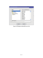
Figure B.4 Load Intersection Data Files Dialogue
B-6
Figure B.5 Intersection Data Files Loaded
Step 4: Click “North-South” radio to tell the program that the balancing is for northsouth direction;
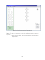
Step 5: Click 4 times
from top to bottom.
icon and we have Figure B.6. The intersections are lined
B-7
Figure B.6 Four Intersections in the Drawing Area
Step 6: Click the top 1st intersection; we have the configuration window as shown in
Figure B.7
Ø Input Intersection Name (An intersection MUST be associated with an
UNIQUE name );
B-8
Figure B.7 Configuring First Intersection
Step 7. ConFigure B.Intersection Legs. Take SB Leg of the first intersection as an
example.
SB Leg, Left turn movement
Ø Select Data Source File from the file list, in this case, select “ CSAH 73 at
No Frontage Rd.txt” (Figure B.11 );
Ø Input “1” in Col Number, as the first data column of “CSAH 73 at No
Frontage Rd.txt” data file corresponds to SB left turn movements ( Figure
B.11);
Ø Check “Lock Left Turn Movement” if SB LT is supposed to be locked
during the balancing process.
Ø Do the same for other movements for SB leg
Ø Do the same for other legs and other intersections.
NOTE:
• The intersection configuration can be saved by “SaveToFile” button, and
existing intersection file can be loaded by “LoadFromFile” Button;
B-9
•
•
For a turning movement that doesn’t actually exist, the user should designate
its Data Source File as empty and Col Number as “ 0”;
When it is desired that some turning movements counts should not changed
during the balancing, the user must designate such movements as “LOCKED”
by checking the respective “Lock XXX turn movement” checkbox (Figure
B.8).
Figure B.8 ConFigure B.SB Intersection Leg
B-10
Figure B.9 ConFigure B.SB Left Turn Movement
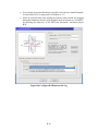
Step 8: After all intersections are configured (Fig 13 ) , click “Check Draw” to check the
geometry.
Figure B.10 Configuration of all intersections done
B-11
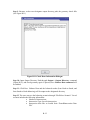
Step 9: Because we have not designate output directory path, the geometry check fails
(See Figure B.11)
Figure B.11 Check Draw Information Dialogue
Step 10: Input Output Directory Path through Output → Output Directory command
(Figure B.12), and check geometry again. If passed, Run → Balnace Data command will
be enabled.
Step 11: Click Run → Balnace Data and the balanced results (from North to South, and
from South to North balancing) will be output to the designated directory.
Step 12: The user can save the balancing scenario through “FileàSave Scenario”. Saved
scenario includes the following information:
§ Number of intersections;
§ Intersection Type for each intersection;
§ Intersection data files as loaded from “DataàIntersection Data
File”
B-12
Figure B.12 Designate Output Directory Path
B-13