Download this introduction

SAGE for Undergraduates:
How to Get Started
Gregory V. Bard
January 17, 2013
Contents
1 Welcome to SAGE!
1.1 Using SAGE as a calculator . . . . . . . . . . . . . . . . . . . . . . . . .
1.2 Using SAGE with Common Functions . . . . . . . . . . . . . . . . . . .
1.3 Using SAGE for trigonometry. . . . . . . . . . . . . . . . . . . . . . . .
1.4 Using SAGE to graph 2-dimensionally. . . . . . . . . . . . . . . . . . . .
1.5 Matrices and SAGE, Part One . . . . . . . . . . . . . . . . . . . . . . .
1.5.1 A First Taste of Matrices . . . . . . . . . . . . . . . . . . . . . .
1.5.2 Complications . . . . . . . . . . . . . . . . . . . . . . . . . . . .
1.5.3 Doing the RREF in SAGE . . . . . . . . . . . . . . . . . . . . .
1.5.4 The Semi-Rare Cases . . . . . . . . . . . . . . . . . . . . . . . .
1.5.5 The Rare Case . . . . . . . . . . . . . . . . . . . . . . . . . . . .
1.5.6 Geometrical Interpretations . . . . . . . . . . . . . . . . . . . . .
1.5.7 Minor Notes . . . . . . . . . . . . . . . . . . . . . . . . . . . . .
1.6 Making your Own Functions in SAGE . . . . . . . . . . . . . . . . . . .
1.7 Using SAGE to Manipulate Polynomials . . . . . . . . . . . . . . . . . .
1.8 Using SAGE to graph a 3-dimensional function, or an implicit function.
1.9 Using SAGE to solve problems symbolically. . . . . . . . . . . . . . . . .
1.10 Using SAGE as a numerical solver. . . . . . . . . . . . . . . . . . . . . .
1.11 Using SAGE to take derivatives . . . . . . . . . . . . . . . . . . . . . . .
1.12 Derivatives and Gradients in Multivariate Calculus . . . . . . . . . . . .
1.13 Using SAGE to calculate integrals, both numerically and symbolically. .
1.14 Matrices in SAGE, Part Two . . . . . . . . . . . . . . . . . . . . . . . .
.
.
.
.
.
.
.
.
.
.
.
.
.
.
.
.
.
.
.
.
.
.
.
.
.
.
.
.
.
.
.
.
.
.
.
.
.
.
.
.
.
.
.
.
.
.
.
.
.
.
.
.
.
.
.
.
.
.
.
.
.
.
.
.
.
.
.
.
.
.
.
.
.
.
.
.
.
.
.
.
.
.
.
.
.
.
.
.
.
.
.
.
.
.
.
.
.
.
.
.
.
.
.
.
.
.
.
.
.
.
.
.
.
.
.
.
.
.
.
.
.
.
.
.
.
.
.
.
.
.
.
.
.
.
.
.
.
.
.
.
.
.
.
.
.
.
.
.
.
.
.
.
.
.
.
.
.
.
.
.
.
.
.
.
.
.
.
.
.
.
.
.
.
.
.
.
.
.
.
.
.
.
.
.
.
.
.
.
.
.
.
.
.
.
.
.
.
.
.
.
.
.
.
.
.
.
.
.
.
.
.
.
.
.
.
.
.
.
.
.
.
.
.
.
.
.
.
.
.
.
.
.
.
.
.
.
.
.
.
.
.
.
.
.
.
.
.
.
.
.
.
.
3
4
5
9
10
17
17
17
19
20
22
22
22
22
24
24
30
35
38
40
41
47
2 Fun
2.1
2.2
2.3
2.4
2.5
2.6
2.7
2.8
2.9
2.10
2.11
.
.
.
.
.
.
.
.
.
.
.
.
.
.
.
.
.
.
.
.
.
.
.
.
.
.
.
.
.
.
.
.
.
.
.
.
.
.
.
.
.
.
.
.
.
.
.
.
.
.
.
.
.
.
.
.
.
.
.
.
.
.
.
.
.
.
.
.
.
.
.
.
.
.
.
.
.
.
.
.
.
.
.
.
.
.
.
.
.
.
.
.
.
.
.
.
.
.
.
.
.
.
.
.
.
.
.
.
.
.
.
.
.
.
.
.
.
.
.
.
.
.
.
.
.
.
.
.
.
.
.
.
48
48
49
50
51
53
53
53
54
54
54
54
Exploration Projects using SAGE
The Pure Math Example: Quintics . . . . . . . . . .
The Finance Example: Mortgages . . . . . . . . . .
The Physics Example: Gravitation and Satellites . .
The Microeconomic Example: Selling Price . . . . .
The Engineering Example: Two-Stage Rockets . . .
The Ecology Example: Lake Dumping . . . . . . . .
The Astronomy Example: Point of Closest Approach
The Earth Science Example: Sunrise and Sunset . .
The Medical Example: Blood in an Artery . . . . . .
The Business Example: a Vehicle Fleet . . . . . . . .
The Biology Example: Predator/Prey Models . . . .
1
.
.
.
.
.
.
.
.
.
.
.
.
.
.
.
.
.
.
.
.
.
.
.
.
.
.
.
.
.
.
.
.
.
.
.
.
.
.
.
.
.
.
.
.
.
.
.
.
.
.
.
.
.
.
.
.
.
.
.
.
.
.
.
.
.
.
.
.
.
.
.
.
.
.
.
.
.
.
.
.
.
.
.
.
.
.
.
.
.
.
.
.
.
.
.
.
.
.
.
.
.
.
.
.
.
.
.
.
.
.
.
.
.
.
.
.
.
.
.
.
.
3 Advanced Features of SAGE
3.1 Using SAGE to work with integers. (gcd, lcm, factorization,
3.2 Minor Commands of SAGE . . . . . . . . . . . . . . . . . .
3.2.1 Rounding, Floors, and Ceilings . . . . . . . . . . . .
3.2.2 Combinations and Permutations . . . . . . . . . . .
3.2.3 Calculating Limits Expressly . . . . . . . . . . . . .
3.2.4 The Hyperbolic Trigonometric functions? . . . . . .
3.3 Scatter Plots in SAGE . . . . . . . . . . . . . . . . . . . . .
3.4 Making Your Own Regressions in SAGE . . . . . . . . . . .
3.5 Additional Topics in Plotting and Graphing . . . . . . . . .
3.6 Graphing Inequalities & Linear Programming . . . . . . . .
3.7 What about Octal? Binary? and Hexadecimal? . . . . . . .
3.8 Can SAGE do Sudoku? . . . . . . . . . . . . . . . . . . . .
3.9 Measuring the Speed of SAGE . . . . . . . . . . . . . . . .
3.10 Huge Numbers and SAGE . . . . . . . . . . . . . . . . . . .
3.11 Advanced Linear Algebra . . . . . . . . . . . . . . . . . . .
3.12 Taylor Series or MacLaurin Polynomials . . . . . . . . . . .
3.13 Super-Advanced Plotting . . . . . . . . . . . . . . . . . . .
3.14 Minimizations and Lagrange Multipliers . . . . . . . . . . .
3.15 Infinite Series, Sums, and Products . . . . . . . . . . . . . .
3.16 Ultra-High Precision Arithmetic . . . . . . . . . . . . . . .
3.17 Using SAGE to work with Cramer’s Rule . . . . . . . . . .
3.18 Using SAGE to work with Resultants . . . . . . . . . . . .
sigma,
. . . .
. . . .
. . . .
. . . .
. . . .
. . . .
. . . .
. . . .
. . . .
. . . .
. . . .
. . . .
. . . .
. . . .
. . . .
. . . .
. . . .
. . . .
. . . .
. . . .
. . . .
tau, etc. . . )
. . . . . . .
. . . . . . .
. . . . . . .
. . . . . . .
. . . . . . .
. . . . . . .
. . . . . . .
. . . . . . .
. . . . . . .
. . . . . . .
. . . . . . .
. . . . . . .
. . . . . . .
. . . . . . .
. . . . . . .
. . . . . . .
. . . . . . .
. . . . . . .
. . . . . . .
. . . . . . .
. . . . . . .
.
.
.
.
.
.
.
.
.
.
.
.
.
.
.
.
.
.
.
.
.
.
.
.
.
.
.
.
.
.
.
.
.
.
.
.
.
.
.
.
.
.
.
.
.
.
.
.
.
.
.
.
.
.
.
.
.
.
.
.
.
.
.
.
.
.
.
.
.
.
.
.
.
.
.
.
.
.
.
.
.
.
.
.
.
.
.
.
.
.
.
.
.
.
.
.
.
.
.
.
.
.
.
.
.
.
.
.
.
.
.
.
.
.
.
.
.
.
.
.
.
.
.
.
.
.
.
.
.
.
.
.
.
.
.
.
.
.
.
.
.
.
.
.
.
.
.
.
.
.
.
.
.
.
.
.
.
.
.
.
.
.
.
.
.
.
.
.
.
.
.
.
.
.
.
.
A Obtaining a SAGE Account
55
55
60
60
60
61
62
62
65
67
74
74
74
75
75
76
77
77
77
77
77
77
78
79
B Convenience Features of SAGE
B.1 Copy and Paste: . . . . . . . . . . . . . . . . . .
B.2 The Moving Slash: . . . . . . . . . . . . . . . . .
B.3 The Online Help System . . . . . . . . . . . . . .
B.3.1 Forgetting Long Commands . . . . . . . .
B.3.2 When You Don’t Know which Command
B.3.3 A Superb Google Trick . . . . . . . . . .
B.4 Inserting a Line/Box . . . . . . . . . . . . . . . .
B.5 Deleting a Line/Box . . . . . . . . . . . . . . . .
B.6 Combining or Splitting Boxes . . . . . . . . . . .
B.7 Manual Restart and Re-Evaluate . . . . . . . . .
B.8 Sharing your Work . . . . . . . . . . . . . . . . .
B.9 Renaming vs Cloning . . . . . . . . . . . . . . . .
B.10 Saving/Loading your Work Locally . . . . . . . .
B.11 Semicolons . . . . . . . . . . . . . . . . . . . . .
B.12 Displaying Source Code . . . . . . . . . . . . . .
.
.
.
.
.
.
.
.
.
.
.
.
.
.
.
.
.
.
.
.
.
.
.
.
.
.
.
.
.
.
.
.
.
.
.
.
.
.
.
.
.
.
.
.
.
.
.
.
.
.
.
.
.
.
.
.
.
.
.
.
.
.
.
.
.
.
.
.
.
.
.
.
.
.
.
.
.
.
.
.
.
.
.
.
.
.
.
.
.
.
.
.
.
.
.
.
.
.
.
.
.
.
.
.
.
.
.
.
.
.
.
.
.
.
.
.
.
.
.
.
.
.
.
.
.
.
.
.
.
.
.
.
.
.
.
.
.
.
.
.
.
.
.
.
.
.
.
.
.
.
.
.
.
.
.
.
.
.
.
.
.
.
.
.
.
.
.
.
.
.
.
.
.
.
.
.
.
.
.
.
.
.
.
.
.
.
.
.
.
.
.
.
.
.
.
.
.
.
.
.
.
.
.
.
.
.
.
.
.
.
.
.
.
.
.
.
.
.
.
.
.
.
.
.
.
.
.
.
.
.
.
.
.
.
.
.
.
.
.
.
.
.
.
.
.
.
.
.
.
.
.
.
.
.
.
.
.
.
.
.
.
.
.
.
.
.
.
.
.
.
.
.
.
.
.
.
.
.
.
.
.
.
.
.
.
.
.
.
.
.
.
.
.
.
.
.
.
.
.
.
.
.
.
.
.
.
.
.
.
.
.
.
.
.
.
.
.
.
.
.
.
.
.
.
.
.
.
.
.
.
.
.
.
.
.
.
.
.
.
.
.
.
.
.
.
.
.
.
.
.
.
.
.
.
.
.
.
.
.
.
.
.
.
.
.
.
.
.
.
.
.
.
.
.
.
81
81
81
81
82
82
82
82
83
83
83
83
83
83
83
83
C Other Resources for SAGE
85
D Installing SAGE on your Personal Computer
86
2
Chapter 1
Welcome to SAGE!
As the open-source and FREE competitor to expensive software like Maple, Mathematica, Magma and
Matlab, SAGE offers anyone with access to a web-browser the ability to use cutting-edge mathematical
software, and display one’s results for others. This document is going to share with you several common
mathematical tasks that are extremely easy, and which may serve as your starting point into SAGE. I’m
sure that you will find SAGE far easier to use than a graphing calculator, and vastly more powerful.
How to Use This Guide
There is no need to read this entire document, just as you would never read the dictionary cover to cover.
If you are handed this guide as part of a class, then your professor will tell you which section numbers
correspond with what you need to know. Personally, I recommend just reading Chapter One, and then start
playing around on your own. Using the find feature of your pdf viewer, you can always search this guide
for whatever command you would like to use. I recommend that you never try to read more than 3 entire
sections in one day. Otherwise there is too much for your brain to absorb while still keeping the experience
fun and new.
Chapter 1 contains the basics—what you really need to know. Chapter 2 has various topics of advanced
mathematics, and its sections are meant to be read independently of each other as needed. Chapter 3 will
cover writing your own programs in SAGE and Python, but it isn’t written yet. The appendices contain lots
of useful information, particularly Appendix C, convenience features of SAGE, and Appendix D which lists
other resources for SAGE. Last but not least, the Table of Contents can be found at the back of the guide,
and serves as an easy substitute for an index.
I assume you do not already have an account on the SAGE notebook server. If you have one, then log
in now, but if not, then see Appendix A, which will tell you how to get an account. In Appendix E are the
directions for installing it on your personal computer, but this a very long and difficult process, and it is not
recommended to beginners.
3
1.1
Using SAGE as a calculator
First off, you can always use SAGE as a simple calculator. For example, if you type 2+3 and click “evaluate”
then you will learn the answer is 5.
The expressions can become as complicated as you like. To calculate the amount on a simple interest
loan at 6% per year for 90 days, and principal $ 900, we all know the formula to be A = P (1 + rt) so we
would just type in
900*(1+0.06*(90/365))
and click “evaluate”. You will learn that the answer is 913.315068493151, or $ 913.32 after rounding to the
nearest penny.
Notice that the symbol for addition is the plus sign, and the symbol for subtraction is the hyphen. The
symbol for multiplication is the asterisk, and the symbol for division is the forward slash (that’s the one
found with the question mark, not the backslash.)
For compound interest, we’d need to take exponents. The symbol for exponents is the caret, found above
the number six on most keyboards. It looks like this “ˆ”.
Let’s consider 12% compounded annually on a signature loan for 3 years, and a principal of $ 11,000. We
all know the formula to be A = P (1 + i)n , and so we would just type in
11000*(1+0.12)^3
and click “evaluate”. You will learn that the answer is 15454.2080000000, or $ 15,454.21 after rounding to
the nearest penny. By the way, instead of clicking “evaluate,” you can just press shift-enter on the keyboard,
and it will do the same thing.
Warning: It is very important not to enter a comma in large numbers when using SAGE. You have to
type 11000 and not 11,000
For those who don’t like the caret, you can use two asterisks in a row.
11000*(1+0.12)**3
which is actually a throw-back to the historical programming language FORTRAN which was most popular1
during the 1970s and 1980s.
What if you make a mistake? Let’s say that I really meant to say $ 13,000 and not $ 11,000. Click on
the mistake, and correct it using the keyboard, and change the 11 into 13. Now click “evaluate” again, and
all is well.
There’s also an “Undo” button and it does exactly what you think it does. However, if you’ve done a lot
of work, you have to scroll the window all the way to the top of the document to find it, as this button sits
at the top of the sheet.
The Red Line: You may have noticed a vertical red line next to the box after you had begun to change
the formula, but before you had clicked “evaluate.” After you have clicked “evaluate,” the red line vanished.
The purpose of this red line is to tell you that the information in the box had changed since the last time
“evaluate” had been clicked, and so you need to hit “evaluate” again to get an accurate answer.
1 An irrelevant historical aside: Because rewriting software is a painful and time-consuming process, many important pieces
of scientific software remained written in FORTRAN until a few years ago, and likewise the same is true of business software in
COBOL. Each new programming language incorporates features of the previous generation of languages, to make it easier to
learn, and accordingly one sees some truly ancient seeds of dead languages once in a while.
4
The Green Rectangle: Also, you may have noticed (if you have a slow internet connection in particular)
a green rectangle that is very thin under the box where you just typed, and next to the red line. This is to
indicate that your web-browser is connecting to the SAGE server, and has made its request, and waiting for
the answer. Do not hit “evaluate” again. On fast connections, the green rectangle will appear and disappear
very rapidly, and you probably will not see it.
Note, if you have a very slow connection, then see “The Moving Slash” on Page 81.
Saving or Printing your Work: We will go into more detail about this later, but for now notice the
“Save” and “Save & Quit” buttons, as well as the “Discard & Quit” button. These do exactly what you
think they do. You can also use the “Print” button to print your work.
Like the undo button, if you’ve done a lot of work, you’ll have to scroll the window all the way to the
top of the document to find it, as this button sits at the top of the sheet.
Shortcut: While I mentioned it before, if you are tired of clicking “evaluate” all the time, you can just
press Shift and Enter at the same time.
Grouping Symbols When there are multiple sets of parentheses in a formula, sometimes mathematicians
use brackets as a type of “super parentheses.” As it turns out, SAGE needs the brackets for other things,
like lists, and so you have to always use parentheses for grouping inside of formulas.
For example, let’s say you need to evaluate
1 − (1 + 0.05)−30
550
0.05
So you should not type
550 [ 1 - (1+0.05)^(-30) ]/0.05
but rather
550 ( 1 - (1+0.05)^(-30) )/0.05
where the brackets have become parentheses.
Some very old math books use braces { and } as a sort of auxiliary also to the parentheses and brackets.
These too, if they are for grouping in a formula, must become parentheses. As it turns out, SAGE, as well
as modern mathematical books, use the braces { and } to denote sets.
By the way, the above formula was not artificial. It is the value of a loan at 5% compounded annually
for 30 years, with an annual payment of $ 550. The formula is called “the present value of an annuity.”
Three Mistakes that are 90+% of My Errors in SAGE: There are three mistakes that I make a lot
when using SAGE. For example, if you want to say 11, 000x + 1200 then you have to type
11000*x+1200
The first error that I sometimes make is that I leave out the asterisk between 11000 and x. In SAGE,
you must include that asterisk, as that is the symbol of multiplication. The second error that I’ll often add
a comma inside the 11000, but it is not acceptable in SAGE to write 11,000 for 11000. The third error is
that I’ll have mismatched parentheses. Any SAGE expression should have the same number of (s as it has
of )s—no more and no less.
1.2
Using SAGE with Common Functions
Now I’ll discuss how SAGE works with square roots, logarithms, exponentials, and so forth.
5
Square Roots: The standard “high school” functions are also built-in. For example, type
sqrt(144)
then click “evaluate” and you’ll learn that the answer is 12. From now on, I’m not going to say “click
evaluate”, because repeating that might get tiresome; I’ll assume that you know you have to do that. Since
SAGE likes exact answers, try
sqrt(8)
and get 2*sqrt(2) as your answer. If you really need a decimal, try instead
N( sqrt(8) )
and obtain
2.82842712475.
which is a decimal approximation.
The N() function, which can also be written n(), will convert what is inside the parentheses to a real
number, if possible. Usually that is a decimal expansion, and so unless what is inside the parentheses is
an integer2 then it will be, necessarily, an approximation. SAGE will assume that all decimals are mere
approximations, so for example
sqrt(3.4)
will evaluate to 1.84390889145858, without need of using N().
Higher Order Roots:
sixth root of 64, do
Higher order roots can be calculated like exponents are. For example, to find the
64^(1/6)
and obtain that the answer is 2.
Getting Both Square Roots: In the spirit of absolute pomposity, you may know that (−2)2 = 4 as well
as 22 = 4. So if you want all the square roots of a number you can do
sqrt(4,all=True)
to obtain
[2, -2]
where the square brackets indicate a list. We’ll see other examples of lists on Page 68, Page 32, Page 57,
and Page 62.
A Taste of the Complex Numbers If you know about complex numbers, you can do
sqrt(-4,all=True)
to obtain
[2*I, -2*I]
√
where the capital letter I represents −1, the imaginary constant. You might be interested to know that
you can use the lowercase i instead of the capital one, if you prefer. While SAGE is quite good at complex
analysis, and can produce some rather lovely plots of functions of a complex variable, we will not go into
those details in this document.
2 To be mathematically correct, I should say “an integer or a fraction with denominator writable as a product of a power
of 5 and a power of 2.” For example, 25ths, 16ths, and 80ths can be written exactly with decimals, where as 3rds, 15ths, and
14th cannot. Observe that 25 = 52 and 16 = 24 as well as 80 = 24 × 5. Those denominators have only 2s and 5s in their
prime factorization. Meanwhile, 3 = 3 and 3 = 5 × 3 while 14 = 7 × 2. As you can see, those denominators have primes other
than 2 and 5 in their prime factorization. If you find this interesting, you should read “Using SAGE to work with Integers” on
Page 55.
6
Special Constants Pi and e: We’ve learned that the imaginary constant is capital “I”. It turns out that
π is built in as “pi” (both letters lower case) and e is built in as “e” (again, lower case).
You can do things like
numerical_approx(pi, prec=200)
to get many digits of pi, or likewise
numerical_approx(sqrt(2), prec=200)
√
to get a high-accuracy expansion of 2. These expansions are to 200 bits, and basically if you want 100
digits, you can do 332 bits; 200 digits3 is 664 bits, and so on. You can also abbreviate with
n(sqrt(2), prec=200)
as we did earlier. That’s what the N() or n() function (they are the same) is an abbreviation of, namely
“numerical approx.”
Is SAGE Case-Sensitive? You’ve probably had a situation in life where you entered your password
correctly, but discovered that it was rejected because you had the wrong capitalization. For example,
perhaps you’ve left the “CAPS-LOCK” key on. In any event, SAGE does think of Pi as different from pi
and Sin as different from sin.
√
The only two exceptions are i and n(). √
First, you can represent −1 as either i or I and either way
SAGE will know what you meant, namely −1. Second, you can write n(sqrt(2)) or N(sqrt(2)) and
SAGE treats those as identical.
√
These easements only apply to −1 and n() as it turns out; in all other cases, capitalization matters.
Tab Completion: Now would be a good time to explain a neat feature of SAGE. If you are typing a long
command, like “numerical approx” and part way through you forget the exact ending (is it approximation?
approximations? appr?) then you can hit the tab button. If only one command in the entire library has
that prefix, then SAGE will fill in the rest for you. If it does not, then you have to enter a few more letters.
On a slow internet connection, the pause can be very noticeable, but it is still a useful feature when you
cannot remember exact commands.
Exponentials:
Just as
2^3
gives you 23 and likewise
3^3
gives you 33 , if you want to say e3 then just say
e^3
and that’s fine. Or for a decimal approximation you can do
N(e^3)
Also, it is worth mentioning sometimes books will write
exp(5 · 11 + 8) instead of e5·11+8
and SAGE thinks that’s just fine. For example,
exp(5*11+8) - e^(5*11+8)
evaluates to 0. Don’t forget the asterisk between the 5 and the 11.
3 This
turns out to be because 10200 ≈ 2664 , if you are curious.
7
Logarithms Of course, SAGE knows about logarithms. But there’s a problem. There are several types of
logarithm, including the common logarithm, the natural logarithm, the binary logarithm, and the logarithm
to any other base you feel like using. In high school and middle school, “log” refers to the common logarithm,
and “ln” to the natural logarithm. However, during and after calculus, “log” refers to the natural logarithm.
Since SAGE was mainly meant for university-and-higher level work, then it is only natural they chose to use
the natural logarithm for “log.”
So to find the natural logarithm of 100 type
N( log(100) )
for the common logarithm of 100 type
N( log(100,10) )
and for the binary logarithm of 100 type
N( log(100,2) )
which of course generalizes. To find the logarithm of 100 base 42, type
N( log(100,42) )
Note that SAGE is quite good at getting exact answers. Try
log ( sqrt(100^3) ,10)
and you will obtain 3, the exact answer.
The Underscore: One of the most useful commands in SAGE is the underscore, and on most keyboards
that can be found by pressing shift and the hyphen or dash. It looks like this:
The numerical value of the special symbol is the value of the previous box. So it is kind of like Ans on
a graphing calculator. For example, you can add 100 to the previous box by typing +100.
One of the ways that I use this is with the n( ) command. Imagine you type sqrt(75) and get back
5*sqrt(3). But suppose you wanted instead a decimal approximation. Then you can type n( ) and SAGE
replies 8.66025403784439.
A Financial Example: Suppose you deposit $ 5000 in an account that earns 4.5% compounded monthly.
You are curious when your total will reach $ 7000. Using the formula A = P (1+i)n , where P is the principal,
A is the amount at the end, i is the interest rate per month, and n is the number of compounding periods
(number of months), we have
7000
=
5000(1 + 0.045/12)n
1.4
=
(1 + 0.045/12)n
log 1.4
=
log(1 + 0.045/12)n
log 1.4
log 1.4
log(1 + 0.045/12)
=
n log(1 + 0.045/12)
=
n
And so, we type into SAGE
log(1.4)/log(1+0.045/12)
and get the response 89.8940609330801, so that we know 90 months will be required. Therefore we write
the answer 7 years and 6 months.
This is an example of a computer-assisted solution to a problem. In addition to that approach, SAGE is
also willing to solve the problem from start to finish, with no human intervention. We’ll see that on Page 38.
8
1.3
Using SAGE for trigonometry.
For trigonometry, SAGE works in radians. So if you want to know the sine of π/3, you should type
sin(pi/3)
and you will get the answer 1/2*sqrt(3). This is an exact answer, rather than a mere decimal approximation.
You will find that SAGE is very oriented toward exact rather than approximate answers. Sometimes this is
irritating, because if you ask for the cosine of π/12, then you would type
cos(pi/12)
and obtain 1/12*(sqrt(3) + 3)*sqrt(6) which is especially irritating if you want a decimal. Instead, if
you type
N(cos(pi/12))
then you will obtain 0.965925826289, a rather good decimal approximation.
You will discover that SAGE is fairly savvy when it comes to knowing when functions will go wrong. In
particular, just try evaluating tangent at one of its asymptotes. For example,
tan(pi/2)
will produce the helpful answer “Infinity.” The “rare” or “reciprocal” trigonometric functions of cotangent,
secant, and cosecant, which are important in calculus but annoying on hand-held calculators, are built into
SAGE. They are identified as cot, sec, and csc.
The inverse trigonometric functions are also available. They are used just like the trigonometric functions.
For example, if you type
arcsin(1/2)
you will obtain
1/6*pi
as expected. Likewise
arccos(1/2)
produces
1/3*pi
The usual abbreviations are all known by and used by SAGE. Here is a complete list:
Math Notation Long-form SAGE command Short-form SAGE command
sin−1 x
arcsin(x)
asin(x)
cos−1 x
arcsin(x)
acos(x)
tan−1 x
arcsin(x)
atan(x)
cot−1 x
arccot(x)
acot(x)
sec−1 x
arcsec(x)
asec(x)
csc−1 x
arccsc(x)
acsc(x)
You can also use SAGE to graph the trigonometric functions. We’ll do that in the section entitled “Using
SAGE to graph 2-dimensionally,” on Page 12
Converting to Degrees, and Back: Remember, to covert radians to degrees, just multiply by 180/π,
and to multiply from degrees to radians, just multiply by π/180. Here’s what you type, to convert π/3 to
degrees:
(pi/3) * (180/pi)
produces
60
while
60 * (pi/180)
produces
1/3*pi
The way I like to remember this is that one protractor is 180 degrees, and protractor begins with “p,”
while π is the Greek “p.” For example, 90 degrees is half a protractor, and 60 degrees is a quarter protractor.
9
That’s why I can remember that they are π/2 and π/2. Likewise, if I see pi/6, then I know that this is
one-sixth of a protractor or 30 degrees.
There is actually an elaborate package in SAGE for converting among different units, and it can be quite
useful. I hope to add it to this document in the near future.
1.4
Using SAGE to graph 2-dimensionally.
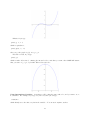
My favorite shape is the parabola, so let’s start there. Type
plot(x^2)
and you get a lovely plot of a parabola going in the range
−1 < x < 1
which is the default range. It will bound the y-values to whatever is needed to show those x-values. Here’s
what you will get:
Likewise you can do
plot(x^3-x)
which is nice and visually appealing, as you can see:
For |x − 1/2| you can do
10
plot(abs(x-1/2))
which can come up from time to time. This produces
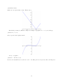
But what if you wanted a different x range? For example, to graph in −2 < x < 2 you would type
plot(x^3-x, -2, 2)
and you get the desired graph, namely:
A very cool graph is
plot(x^4 - 3*x^2+2,-2,2)
but notice the asterisk between 3 and x in “ 3*x ”. You will get an error if you leave that out! The plot is
11
Another minor sticking point is that for y = sin(t) you have to say
plot(sin(x))
or better yet
plot(sin(x),-10,10)
because plot is not expecting t, it expects x. The images that you get are
plot(sin(x))
plot(sin(x),-10,10)
In fact if you were to type
plot(sin(t))
you would see
Traceback (click to the left of this block for traceback)
...
NameError: name ’t’ is not defined
because in this case, SAGE does not know what ’t’ means. An alternative way of handling this is given on
Page 29.
Going “Off the Scale”:
Consider the plot of x3 from x = 5 to x = 10, which is given by
plot(x^3, 5, 10)
12
and as you can imagine, the function goes from 53 = 125 up to 103 = 1000, and so the origin should appear
very far below the graph. This is the plot:
Your hint that the location of the x-axis in the display is not where it would be normally is that the axes
do not intersect. This is to tell you that the origin is far away. When the axes do intersect on the screen,
then the origin is (both in truth and on the screen) where they intersect. Also, if you want to, you can hide
the axes with
plot(x^3, 5, 10, axes=false)
and that produces
which is considerably less informative.
To Force the Y-Range of a Graph: If, for some reason, you want to force the y-range of a graph to be
constrained between two values, you can do that. For example, to keep −6 < y < 6, we can do
plot( x^3-x, -3, 3, ymin = -6, ymax = 6)
in order to obtain
13
This is important, because normally SAGE wants to show you the entire graph. Therefore, it will make
sure that the y-axis is tall enough to include every point, from the maximum to the minimum. For some
functions, either the maximum or the minimum or both, could be huge.
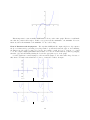
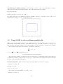
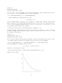
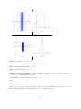
Plots of Functions with Asymptotes: The way that SAGE (and all computer algebra tools) computes
the plot of a function is by generating a very large number of points in the interval of the xs, and evaluating
the function at each of those points. To be precise, if you want to graph f (x) = 1/x2 between x = −4 and
x = 4, the computer might pick 10,000 random values of x between −4 and 4 find the y values by plugging
them into f (x) and then finally drawing the dots in the appropriate spots on the graph.
So if the graph has a vertical asymptote, then near that asymptote, the value will be huge. Because of
this, when you graph a rational function, be sure to restrict the y-values. Compare:
Plot 1
Plot 2
Plot 3
Plot 4
14
Plot 1:
plot(1/(x^3-x), -2, 2)
Plot 2:
plot(1/(x^3-x), -2, 2, ymin = -5, ymax = 5)
Plot 3:
plot(1/(x^3-x), (x,-2, 2),detect_poles=true, ymin = -5, ymax = 5)
Plot 4:
plot(1/(x^3-x), (x,-2, 2),detect_poles=’show’, ymin = -5, ymax = 5)
As you can see, the first is a disaster. The second one cuts off the very-high and very-low y-values, but it
keeps trying to connect the various “limbs” of the graph. When you set “detect poles” to true, then it will
figure out that the pieces are not connected.
One minor point. Did you notice in the four plots above, that ’show’ is in quotes, but true is not in
quotes? That’s because true and false occur so often in math, that they are built-in keywords in SAGE.
However, the ’show’ occurs less often, and therefore is not built in, and we must put it in quotes, just as
we do with colors while plotting.
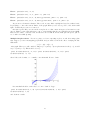
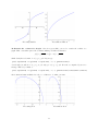
Multiple Graphs at Once: Now we’re going to see how to superimpose plots on each other, using a plus
sign. Suppose you were investigating polynomials, and you wanted to know the effect of varying the last
numeral in
y = (x − 1)(x − 2)(x − 5)
on its graph. Then you could consider looking at (x − 3) and (x − 4) as replacements for the (x − 5), as well
as (x − 6) and (x − 7). This would be done by
plot( (x-1)*(x-2)*(x-3), -2, 10) + plot( (x-1)*(x-2)*(x-4), -2, 10) + plot(
(x-1)*(x-2)*(x-5), -2, 10)
where I chose the domain, x = −2 until x = 10, arbitrarily. Now we obtain
It seems that I should zoom in a bit, to see more detail. So I type
plot( (x-1)*(x-2)*(x-3), 1, 6) + plot( (x-1)*(x-2)*(x-4), 1, 6) + plot(
(x-1)*(x-2)*(x-5), 1, 6)
and obtain as a result
15
Now I can see better what that last numeral does. It controls the location, or x-coordinate, of the last
time that the curve crosses the x-axis. As you can see, the plus sign among the plot commands means to
superimpose them.
There is a technicality here. You must not break a newline among the plots and plus signs. The various
plot commands and their plus signs must be strung together, like a paragraph, wrapping naturally from one
line to the next. You do not use the enter key to put each plot on its own line. Thus, you cannot do:
plot( (x-1)*(x-2)*(x-3), 1, 6)
+ plot( (x-1)*(x-2)*(x-4), 1, 6)
+ plot( (x-1)*(x-2)*(x-5), 1, 6)
+ plot( (x-1)*(x-2)*(x-6), 1, 6)
+ plot( (x-1)*(x-2)*(x-7), 1, 6)
which SAGE thinks is five separate commands, instead of one big command.
Therefore, if you have problems getting those last two commands to work, then check to see that you
have no accidental “line breaks” in the command. For SAGE, these commands must be entered without a
line break, kind of like typing a long paragraph in an ordinary word processor—you can wrap around the
end of the line, but you cannot insert a line break.
Further Graphing & Plotting Topics The following additional topics on graphing and plotting can be
found in the section “Advanced Topics in Plotting and Graphing” on Page 67. They include
• Graphing with Colors.
• Labels and Legends.
• Grids and Graphing Calculator-Style Graphs.
• Labeling the Axes of Graphs.
• Graphs of Hyperactive Functions.
• Odd Roots of Negative Numbers.
• Restricting the X-Range of Plots.
16
1.5
1.5.1
Matrices and SAGE, Part One
A First Taste of Matrices
This section assumes that you’ve never worked with matrices before in any way, or alternatively, that you
have forgotten them. Experts in linear algebra can skip to the next subsection “Doing the RREF in SAGE.”
Let us suppose that you wish to solve the following linear system of equations:
3x − 4y + 5z
=
14
x + y − 8z
= −5
2x + y + z
=
First you would convert this into the following

3
A= 1
2
7
matrix:
−4
1
1
5
−8
1

14
−5 
7
Notice that the coefficients of the xs all appear in the first column; the coefficients of the ys all appear
in the second column; the coefficients of the zs all appear in the third column. The fourth column gets the
constants. Thus we have encapsulated and abbreviated all of the information of the problem. Furthermore
observe that additions are represented by a positive coefficient, and subtractions by a negative coefficient.
Matrices have a special form called “Reduced Row Echelon Form” often abbreviated as RREF. The
RREF is, from a certain perspective, the simplest description of the system of equations that is still true.
The Reduced Row Echelon Form of this matrix A is


1 0 0 3
 0 1 0 0 
0 0 1 1
We can translate this literally as
1x + 0y + 0z
=
3
0x + 1y + 0z
=
0
0x + 0y + 1z
=
1
or in simpler notation
x=3
y=0
z=1
which is the answer. You should take a moment now, plug in these three values, and see that it comes out
correct.
1.5.2
Complications
You might be looking at the previous discussion and imagine that what we’re doing is a kind of silver-bullet,
quickly capable of solving any of a large number of extremely tedious problems that take (with a pencil) a
very long time.
Indeed it is, now that we have computers. Prior to the computer, large linear algebra problems were
considered extremely unpleasant. Yet, now that we have computers, and because computers can carry out
these operations essentially instantly, this topic is a great way to rapidly solve enormous systems of linear
equations. That, in turn, means that skilled mathematicians can address important problems in science and
industry, because real-world problems often have many variables.
This topic, however, is better described as “semi-automatic” rather than “automatic.” The reason I say
that is because the human must be very careful to first convert the word problem into a system of linear
17
equations. We will not cover that here. The second step is to convert that system into a matrix, and that
isn’t quite trivial. In fact, it is often the case that student errors occur in this step, and so we will invest a
bit of time with a detailed example.
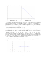
Consider the system of equations:
2x − 5z + y
=
6+w
5+z−y
=
0
w + 3(x + y)
=
z
1 + 2x − y
=
w − 3x
As it turns out, this system of equations has the following traps:
• In the first equation, the variables are out of order, which is extremely common. Very often, both
students and professional mathematicians will fail to notice this, and put the wrong coefficients in the
wrong places. You can use any ordering that you want, so long as you use the same ordering for every
equation. However, to avoid making an error, mathematicians usually put the variables in alphabetical
order.
• Also in the first equation, the w is on the wrong side, and we must move it to the left of the equal
sign. It is necessary that all the variables end up on one side of the equal sign, and all the numbers on
the other side of the equal sign. With these two repairs, the first equation is now
−w + 2x + y − 5z = 6
• The second equation has the constant on the wrong side, and so we must move it across the equal sign,
remembering to negate it.
• As if that were not enough, both x and w are missing in the second equation. We treat this as if the
coefficients were zero. With these two repairs, the second equation is now
0w + 0x − y + z = −5
• The third equation has parentheses. That’s not allowed. We have to remember that 3(x+y) = 3x+3y.
Furthermore, the z is on the wrong side.
• A third “sin” in the third equation is that there is no constant. We treat this as a constant of zero.
Correcting these three issues, we have
w + 3x + 3y − z = 0
• Now the real delinquent is the fourth equation. We have w on the wrong side, and what is worse is
that there are two occasions of x. When we move the −3x from the right of the equal sign to the left,
it becomes +3x and combines with the +2x that was already there, to form 5x. As if that were not
enough, the constant is on the wrong side. Last but not least, z is entirely absent. Correcting all this,
we have
−w + 5x − y + 0z = −1
With these equations in mind, we have the matrix:

−1 2 1
 0 0 −1

B=
1 3 3
−1 5 −1
18
−5
1
−1
0

6
−5 

0 
−1
That would be very tedious to solve by hand using matrices; it would be far worse to solve it by hand
without matrices, using medieval algebra. However, using SAGE, we will solve it in the next subsection. For
now, it turns out that the answer is
w = −107/7
x = −12/7
y = 54/7
z = 19/7
which you can easily verify now if you like.
1.5.3
Doing the RREF in SAGE
This subsection is going to tell you how to compute the RREF of a matrix, presumably with the goal of
solving some linear system of equations. Doing this in SAGE requires only four steps, the last of which is
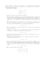
optional. First, we’re going to define the matrix


3 −4 5
14
A =  1 1 −8 −5 
2 1
1
7
which came from the previous subsection. As you can see, it has 3 rows and 4 columns. We’ll do that with
the SAGE command
A = matrix( 3, 4, [ 3, -4, 5, 14, 1, 1, -8, -5, 2, 1, 1, 7 ] )
The key to understanding that SAGE command is to see that the first number is the number of rows,
followed by the number of columns4 . Then follows a list of all the entries, separated by commas, and enclosed
in brackets.
Notice that SAGE does not respond when this command is given. The only reaction is the green rectangle
which appears and disappears. The second step is to verify that the matrix you typed was the matrix that
you had hoped to enter. This step is not avoidable, as typos are extremely common. To do this, just type A
in an empty box by itself. Then the matrix displays, and you can verify that you have typed what you had
wanted to type.
The third step is that you want to compute the RREF or “Reduced Row Echelon Form.” This is done
with the command
A.rref( )
and SAGE tells you the Reduced Row Echelon Form, or


1 0 0 3
 0 1 0 0 
0 0 1 1
The fourth, and optional step, is to check your work, but I highly recommend it! First we type
3*3 + -4*0 + 5*1
and learn that the answer is 14. Next we type
1*3 + 1*0 - 8*1
and learn that the answer -5. The last one is checked similarly.
Note that it is crucial to check all three equations! Otherwise, you’d fail to detect the “imposter” solution
x = 30
y = 29
z=8
which satisfies the first two equations, but not the third one.
4 This is how I remember: Columns, such as on a bank, Congress, or a Greek temple, are vertical. Rows, by process of
elimination, are horizontal. But do we enter the rows first? or the columns first? I always think “RC Cola,” a minor brand of
soda, which reminds me rows-first-columns-second. Thankfully, there does not exist a “CR Cola.”
19
Now let’s consider the “complicated” example

−1
 0
B=
 1
−1
from the previous subsection. It was

2 1 −5 6
0 −1 1 −5 

3 3 −1 0 
5 −1 0 −1
and we can enter that into SAGE with
B = matrix( 4, 5, [-1, 2, 1, -5, 6, 0, 0, -1, 1, -5, 1, 3, 3, -1, 0, -1, 5, -1, 0, -1 ] )
By the way, be certain to enter that above all on its own line. You cannot have any linebreaks. Then
we check with B alone in its own box, and check to see that we have entered that which we had intended to
enter. That being done, we type
B.rref()
into a box and we then learn


1 0 0 0 −107/7
 0 1 0 0 −12/7 


 0 0 1 0
54/7 
0 0 0 1
19/7
Giving the final answer
w = −107/7
x = −12/7
y = 54/7
z = 19/7
Now we must check our work. For example, we check the first equation with
2*(-12/7) - 5*(19/7) + 54/7
and
6 + -107/7
both of which come out to -65/7. The point is not that they come out to -65/7, but rather that they come
out equal. Thus the first equation is satisfied. We check the other three equations similarly.
We really do have to plug each of the four values into each of the four equations, by the way. For example,
the “imposter” solution
w = −139/7
x = −8/7
y = 64/7
z = 29/7
satisfies the first three of those equations, but fails to satisfy the last one.
If you happened to read the previous subsection, you will recall that we did quite a lot of work to get B.
Those many steps might have contained an error if we were sloppy. That’s another reason that we should
check our work.
1.5.4
The Semi-Rare Cases
Now we’re going to examine the two semi-rare cases. These occur if there is one row of all zeros at the
bottom of the matrix, ending in either a non-zero number, or ending in zero. The system of equations is
That results in the matrix
x + 2y + 3z
=
7
4x + 5y + 6z
=
16
7x + 8y + 9z
=
24

1
C1 =  4
7
2
5
8
20
3
6
9

7
16 
24
and that we shall enter into SAGE with
C1 = matrix( 3, 4, [1, 2, 3, 7, 4, 5, 6, 16, 7, 8, 9, 24] )
To find the “solution,” we type
C1.rref( )
and receive back
[
[
[
1
0
0
0
1
0
-1
2
0
0 ]
0 ]
1 ]
This translates into
x−z
=
0
y + 2z
=
0
0
=
1
Now, we’ll examine shortly how to think about those top two equations. However, the bottom equation
says 0 = 1, which is clearly not true! There is no way to satisfy the requirement that 0 = 1. Therefore, this
equation has no solutions. Instead of “the answer” being a solution, a list of solutions, or infinitely many
solutions, the answer is the words “this system has no solutions.” That will be the outcome whenever the
RREF has a row with all zeros except the last column, which is a non-zero number. Whenever you see a
row with all zeros, except in the last column, you must remember that the system has no solutions.
Another interesting case is to change the 24 in the last equation to 25. That results in the matrix


1 2 3 7
C2 =  4 5 6 16 
7 8 9 25
and that we shall enter into SAGE with
C2 = matrix( 3, 4, [1, 2, 3, 7, 4, 5, 6, 16, 7, 8, 9, 25] )
To find the “solution,” we type
C2.rref( )
and receive back
[
[
[
1
0
0
0
1
0
-1
2
0
0 ]
0 ]
0 ]
As you can see, this RREF has a row of all zeros, ending in a zero. That indicates infinitely many solutions.
Some instructors allow you to write “infinitely many solutions” and in certain application problems you would
not care to provide a way of saying what those solutions are.
However, most of the time, you’d like to know what the solutions are. This is especially true in industrial
problems. In any case, you can’t make a list, because there infinitely many of them. Instead, mathematicians
use a dummy variable, usually t, to get around the problem.
Did you notice how the RREFs of A and B all have a certain structure to the matrix? In particular, all the
columns (excepting the last column) have zeros everywhere, except a very noticeable diagonal of ones. Here,
in C2 and C1 as well, we see that column three differs from this pattern. That column is called defective,
and its variable is going to be called “the free variable.” Every other variable will be a formula in terms of
the free variable.
In our case
x−z = 0
x=z
y + 2z = 0
⇒
the final answer
y = −2z
0 = 0
21
though I like to add the words “z is free” to the final answer, under the equations for x and y, even though
it is obvious.
Now what does all this mean? It means that you can choose any z that you want, whatsoever. Once you
have chosen such a z, then you can use those formulas for x and y to make a solution. There is one solution
for every z. Some examples include
If z = 3 then x = z = 3 and y = −2z = −2(3) = −6. The solution is x = 3, y = −6, z = 3.
If z = 2 then x = z = 2 and y = −2z = −2(2) = −4. The solution is x = 2, y = −4, z = 2.
If z = 1 then x = z = 1 and y = −2z = −2(1) = −2. The solution is x = 1, y = −2, z = 1.
If z = 0 then x = z = 0 and y = −2z = −2(0) = 0. The solution is x = 0, y = 0, z = 0.
If z = −1 then x = z = −1 and y = −2z = −2(−1) = 2. The solution is x = −1, y = 2, z = −1.
If z = 4.21 then x = z = 4.21 and y = −2(4.21) = −8.42. The solution is x = 4.21, y = −8.42, z = 4.21.
And so forth, for infinitely many solutions.
1.5.5
The Rare Case
Coming soon!
1.5.6
Geometrical Interpretations
Coming soon!
1.5.7
Minor Notes
Coming soon!
1.6
Making your Own Functions in SAGE
It is extremely easy to define your own functions in SAGE. To me, this is one of the most brilliant design
features of SAGE, that the creators made this very easy for the user. You can make your own function using
exactly the symbols that you would normally use in writing the function down with your pencil.
Defining your own Functions:
If you want to define f (x) = x3 − x then you type
f(x) = x^3-x
and likewise if you wanted to define g(x) =
√
1 − x2 you would type
g(x) = sqrt( 1-x^2 )
which can be very handy.
Take a moment and see that f (0) and f (2) as well as g(0) do exactly what you expect them to do.
Plotting Functions: Now that we’ve defined f (x) and g(x), we can plot them with
plot( f, -2, 2 )
you get the expected plot
22
Likewise if you type
plot( g, 0, 1 )
which is equivalent to
plot( g(x), 0, 1 )
then you get the graph of g(x) on 0 ≤ x ≤ 1.
Last but not least, if you type
plot( g )
which is rather abbreviated—omitting the interval of the x-axis that you want—then SAGE will assume
that you want −1 ≤ x ≤ 1, by default. This produces the plot
Using Intermediate Variables: Sometimes you’ll be using the same value a lot, and you want to store
it somewhere. For example, if you type 355/113 a lot, then you can type
c=335/113
which silently stores the value 335/113 in the variable c. You can use it anytime, such as
23
2+c
which evaluates to 561/113. If you go back and change the value of c however, you have to make sure you
use the “evaluate” button to re-evaluate all other boxes that make use of c. In general, it is easy to avoid
this by not changing intermediate variables once you set them. You can also just tell SAGE to re-evaluate
every single box, in order. This is described on Page 83.
If we wanted to find the relative error of c as an approximation of π we would remember the formula
relative error =
approximation − truth
truth
and type
N((c-pi)/pi)
and learn that the relative error is around 84 parts per billion. Not bad. This approximation was found by
the Chinese Astronomer Zu Chongzhi, also known as Tsu Ch’ung-Chih. We can compare 335/113 to 22/7
with
N((22/7-pi)/pi)
and learn that this much more common approximation of π as 22/7 has a relative error around 402 parts
per million. Much worse!
The intermediate variables technique is great for things like the strength of gravity in physics, or the
speed of light, which (so far as we know) do not change. For things that do change, try “substitution”, which
I’ll tell you about in just a moment. In finance, you could use this for interest rates or the coefficients in a
cost function.
1.7
Using SAGE to Manipulate Polynomials
Coming Soon!
Meanwhile, here is a command list, if you need to look up the commands:
• factor
• expand
• combine and collect
• gcd
• lcm
• adding and subtracting polynomials
• multiplication of polynomials
• how to do polynomial long division
• composition of polynomials
1.8
Using SAGE to graph a 3-dimensional function, or an implicit
function.
Three-dimensional images are not only visually stimulating, but they can help demonstrate a lot of important
effects in the multivariate calculus. Instead of f (x), we will have functions of the form f (x, y). Before, we
had only one variable x, and now we’re adding in the variable y.
This means we need the variable y, so we first type
24
var(’y’)
and now y is declared. The declaration of variables will be explained on Page 31, in case you are curious,
but for now just type it. In general, you need to declare every variable that you use, except that x is so
commonly used so it is built in.
If we wanted to view the bottom part of the paraboloid
z = x2 + y 2
with x and y both ranging from -2 to 2, we would type
var(’y’)
plot3d( x^2 + y^2, (x, -2, 2), (y, -2, 2) )
to obtain
Try that, and try dragging the plot around with the mouse. You can view the plot from all sorts of angles
and directions. Now we can view things from -4 to 4 instead with
plot3d( x^2 + y^2, (x, -4, 4), (y, -4, 4) )
to obtain
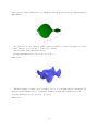
For a hyperbola of one sheet, try
plot3d( x^2 - y^2, (x, -2, 2), (y, -2, 2), color=’green’ )
25
where you can see that we changed the color, just like we did in the previous section on 2-dimensional plots.
This results in
Note, that we do not type var(’y’) again, because you only have to declare each variable once. Once
you have declared it, you do not have to declare it a second time.
And for a surface that is just plain weird, try
plot3d(sin(x-y)*y*cos(x),
(x,-3,3),
(y,-3,3)
)
which creates
This is an example of a surface that you really do have to see from many angles to understand. Try
dragging it around with the mouse to see what it looks like from many angles. Another neat one is
plot3d( 4*x*exp(-x^2-y^2), (x,-2,2), (y,-2,2))
which creates
26
Clearly, this too is a surface that can only be understood by rotating the object and examining it from
several angles.
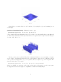
Questions of Resolution Density
plot3d(sin(x-y)*y*cos(x),
If instead you were to type
(x,-10,10),
(y,-10,10)
)
you get a much rougher, irregular surface that does not seem to properly resemble the previous. After all,
we didn’t change the function, and we just went from the 6 × 6 region about the origin to the 20 × 20 region
about the origin. Have a look:
The issue comes down to resolution. The plot3d command by default chooses a certain number of points,
by some method, and samples the function at those points. Whatever method it uses—which is not known
to me—produced enough points for a good 6 × 6 picture, but not enough for a good 20 × 20 picture. The
situation is much improved by typing
plot3d(sin(x-y)*y*cos(x),
(x,-10,10),
(y,-10,10),
plot_points=90 )
which forces SAGE to use 90 points on the x-axis, and 90 points on the y-axis, for a total of 8100 points.
To exaggerate the effect for the purposes of explanation, consider the following images
27
with plot points=90
(that’s 8100 points)
with plot points=30
(that’s 900 points)
Perhaps you might be wondering why we do not always use “a large number” of points. Well, even with
90, you might find that your internet connection slows down, and your computer starts acting slowly, unless
you have a large amount of memory. These 3D-plots require an enormous amount of computation power,
especially if you rotate them.
Implicit Functions Sometimes, in calculus texts, a function is defined implicitly, instead of explicitly.
What I mean is that instead of z = f (x, y) one could have some polynomial, for instance, in x, y, and z
equal to zero. An example might be
4x2 (x2 + y 2 + z 2 + z) + y 2 (y 2 + z 2 − 1) = 0
This should not be too surprising. After all, while most functions in the univariate calculus are defined
as y = f (x), on the other hand, we write a circle like x2 + y 2 = 4, or alternatively x2 + y 2 − 4 = 0 as a
polynomial in x and y, set equal to zero.
In any case, here’s what you would do in SAGE. First, we define the function that we wish to draw:
f(x,y,z) = 4*x^2 *(x^2+y^2+z^2+z) + y^2*(y^2+z^2-1)
Now the following command will plot the set of points where f (x, y, z) = 0, and the variables range over
the values −1/2 < x < 1/2 and −1 < y < 1 as well as −1 < z < 1.
implicit_plot3d( f, (x, -0.5, 0.5), (y, -1, 1), (z, -1, 1), color = ’red’ )
That produces this:
28
Before we wrap up our discussion of 3D plots, it is important to point out that if you were to use
plot points=100 in the above command, then the x-interval would be divided into 100 parts, as well as the
y and z intervals, for a total of
100 × 100 × 100 = 1, 000, 000
plotting points. This is extremely unwise, and can crash your web browser.
Backwards Compatibility
mand’s syntax:
The following syntax makes the plot command look like the plot3d com-
plot( x^2, (x, -2, 2) )
where as we would normally have typed
plot( x^2, -2, 2 )
as in the last section. This useful for when you have to plot things in terms of t and not in terms of x. For
example:
var(’t’)
plot( -16*t^2+400, (t, 0, 3) )
is the height of a bowling ball dropped off of a 400 foot building, t seconds after release. Here is the plot:
29
Two-Dimensional Implicit Plotting Once in a while, you have to plot a curve implicitly, even in two
dimensions. The syntax is basically identical to three-dimensional plots. For example,
g(x,y)=x^4+y^4-16
implicit_plot(g, (x,-3,3), (y,-4,4) )
is a quartic curve favored by furniture designers for making conference room tables. As you can see, its
mathematical formula is x4 + y 4 = 16. Here is the plot:
1.9
Using SAGE to solve problems symbolically.
When we say that a computer has solved a problem for us, that can come out to be in one of two flavors:
symbolically, or numerically. When we solve numerically, we get a decimal expansion for a (very good)
approximation of the answer. When we solve symbolically, we get an exact answer, often in terms of radicals
or other complicated functions. It is a matter of saying if the solutions to
x2
−x−2=0
2
are 1 +
√
5 and 1 −
√
5 or saying that they are
−1.23606797749979 and 3.23606797749979
The former is an example of a symbolic solution, and the latter of a numerical solution. If the answer is
a formula, then symbolic solution is the only way to go. This section is about symbolic solution, and then
the next one is about numerical solution.
Univariate Formulae First, let’s try solving some single-variable problems. We can type
solve(x^2 + 3*x+2, x)
and then we obtain
[x == -2, x == -1]
But don’t forget the asterisk! To be precise, to type
solve(x^2 + 3x+2, x)
30
would be wrong, because of the absence of the asterisk between the “3” and the “x.” Another, more
illustrative of a symbolic computation is
solve(x^2+9*x+15==0,x)
which gives
[x == -1/2*sqrt(21) - 9/2, x == 1/2*sqrt(21) - 9/2]
One way to really see what symbolic versus exact is about is to compare
3+1/(7+1/(15+1/(1+1/(292+1/(1+1/(1+1/6))))))
which returns 1,354,394 / 431,117 with
n(3+1/(7+1/(15+1/(1+1/(292+1/(1+1/(1+1/6)))))))
which returns 3.14159265350241. That could easily be mistaken for π. In fact it is really close to π with
relative error 2.78 × 10−11 .
There is no restriction to polynomials. You can also
var(’theta’)
solve(sin(theta)==1/2, theta)
to get
[theta == 1/6*pi]
You might be confused to see that var command. The idea is that you need to tell SAGE that this
variable is not yet known. We’ve used variables before, but that’s because we had assigned values to them.
When you want a variable to represent some unknown quantity, you must use var. The variable x is always
pre-declared, you do not need to declare it—SAGE assumes that x is an unknown.
Multivariate Formulae Now we’re going to use SAGE to re-derive the quadratic formula. First we must
declare our variables with:
var(’a b c’)
and then we type
solve( a*x^2 + b*x + c == 0, x )
and get instead back
[x == -1/2*(b + sqrt(-4*a*c + b^2))/a,
x == -1/2*(b - sqrt(-4*a*c + b^2))/a]
which has some terms in an unusual order but is undoubtedly correct. Note that the square brackets and
comma indicate a list in SAGE, something which SAGE inherited from the computer language Python.
Declaring Variables in Bulk
By the way
var(’a b c’)
is merely an abbreviation for
var(’a’)
var(’b’)
var(’c’)
Also note that the following for forms are equivalent
var("a, b, c")
var("a b c")
var(’a b c’)
and you can use which ever one you prefer.
31
var(’a, b, c’)
Linear Systems of Equations You can solve several equations simultaneously, whether they are linear
or non-linear. An easy case might be to solve
x+b =
6
x−b =
4
which would be done by typing
var(’b’)
solve( [x+b == 6, x-b == 4], x, b )
Again, note the useof square brackets and commas to form a list in SAGE. This is our second example
of a list in SAGE. You can enclose any data with [ and ], and separate the entries with commas, to make
a list. Our first example, was in graphing multiple functions at once, on Page 68; we’ll see another example
in Number Theory on Page 57, and in scatter plotting live data, on Page 62.
Also, it is important to point out that there is no harm in “declaring” b twice. The two var commands do
no harm to each other. On the other hand, there is also no need to “declare” b twice, as once it is declared,
SAGE will remember that it is a variable.
A more typical linear system might be
9a + 3b + 1c =
32
4a + 2b + 1c =
15
1a + 1b + 1c =
6
and to solve that we’d type
var(’a, b, c’)
solve( [9*a + 3*b + c == 32, 4*a + 2*b + c == 15, a + b + c == 6], a, b, c )
and SAGE gives the answer
[[a == 4, b == -3, c == 5]]
which is correct. Of course, this is exactly the linear system of equations that you would use if someone
asked you to find the parabola connecting the points (3, 32) and (2, 15) as well as (1, 6). That would be
f (x) = 4x2 − 3x + 5.
Naturally, linear systems of equations can also be solved with matrices. In fact, SAGE is quite useful
when working with matrices, and can remove much of the tedium normally associated with matrix algebra.
That will be discussed in the matrix section on Page 17.
Non-Linear Systems of Equations While linear equations are very easy to solve via matrices, the
non-linear case is usually much harder.
First, we will warm up with just one equation, but a highly-non-linear one. Let us try to solve
x6 − 21x5 + 175x4 − 735x3 + 1624x2 − 1764x + 720 = 0
which can be done by
solve( x^6 - 21*x^5 + 175*x^4 - 735*x^3 + 1624*x^2 - 1764*x + 720 == 0, x)
which gives
[x == 5, x == 6, x == 4, x == 2, x == 3, x == 1]
32
That is a list of six answers, because that degree six polynomial has six roots. It was easy to read this
time, but you can also access each answer one at a time. Instead, we type
answer = solve( x^6 - 21*x^5 + 175*x^4 - 735*x^3 + 1624*x^2 - 1764*x + 720 == 0, x)
and then we can type print answer[0] or print answer[1] to get the first or second entries. To get the
fifth entry of that list, we’d type print answer[4]. This is because SAGE is built out of Python, and
Python numbers its lists from 0 and not from 1. There are reasons for this, based on some very old computer
languages.
Now consider this problem, suggested by Dr. Grout. To solve
p+q
=
9
qy + px
= −6
2
2
=
24
p
=
1
qy + px
we would type
var(’p q y’)
eq1 = p+q == 9
eq2 = q*y + p*x == -6
eq3 = q*y^2 + p*x^2 == 24
eq4 = p == 1
solve( [eq1, eq2, eq3, eq4 ], p, q, x, y )
which produces
[[p == 1, q == 8, x == -4/3*sqrt(10) - 2/3, y == 1/6*sqrt(2)*sqrt(5) 2/3], [p == 1, q == 8, x == 4/3*sqrt(10) - 2/3, y ==
-1/6*sqrt(2)*sqrt(5) - 2/3]]
As you can see, that is a list of lists, again using square brackets and commas. Clearly, that is a very
hard to read mess. Using the technique that we learned when analyzing the degree six polynomial above,
we replace the last line with
answer=solve( [eq1, eq2, eq3, eq4 ], p, q, x, y )
Now we can type
print answer[0]
print answer[1]
and we get
[p == 1, q == 8, x == -4/3*sqrt(10) - 2/3, y == 1/6*sqrt(2)*sqrt(5) 2/3]
[p == 1, q == 8, x == 4/3*sqrt(10) - 2/3, y == -1/6*sqrt(2)*sqrt(5) 2/3]
This is SAGE’s way of telling you:
√
Solution 1: p = 1, q = 8, x = − 43 10 − 23 , y =
Solution 2:
p = 1, q = 8, x =
4
3
√
10 − 23 , y = −
√
10
6
−
2
3
−
2
3
√
10
6
Since there are only two answers, we cannot ask for a third. In fact, if we type print answer[2] then
we get
33
Traceback (click to the left of this block for traceback)
...
IndexError: list index out of range
which is SAGE’s way of telling you that it has already given you all the answers for that problem—the list
does not contain a 3rd element.
2
2
Now let’s try to intersect the hyperbola x2 − y 2 = 1 with the ellipse x4 + y3 = 1. We type
var(’y’)
solve([x^2-y^2==1,
(x^2)/4+(y^2)/3==1],x,y)
and obtain
[x == -4/7*sqrt(7), y == -3/7*sqrt(7)], [x == -4/7*sqrt(7), y ==
3/7*sqrt(7)], [x == 4/7*sqrt(7), y == -3/7*sqrt(7)], [x == 4/7*sqrt(7),
y == 3/7*sqrt(7)]]
which is unreadable. Once again, we change the command to be
answer=solve([x^2-y^2==1,
(x^2)/4+(y^2)/3==1],x,y)
and then type
print
print
print
print
print
answer[0]
answer[1]
answer[2]
answer[3]
answer[4]
and that produces four answers and an error message
[x == -4/7*sqrt(7), y == -3/7*sqrt(7)]
[x == -4/7*sqrt(7), y == 3/7*sqrt(7)]
[x == 4/7*sqrt(7), y == -3/7*sqrt(7)]
[x == 4/7*sqrt(7), y == 3/7*sqrt(7)]
Traceback (click to the left of this block for traceback)
...
IndexError: list index out of range
which is SAGE’s way of telling you
√
x=
4
7
Solution 2:
x=
4
7
Solution 3:
√
√
x = − 47 7, y = 37 7
Solution 4:
√
√
x = − 47 7, y = − 37 7
√
7, y =
3
7
√
Solution 1:
7
√
7, y = − 37 7
but that there is no “Solution 5.”
Last but not least, note that we aren’t limited to polynomials. We can do
solve(sin(x+y)==0.5,x)
and obtain
[x == 1/6*pi - y]
34
Complex Numbers: Normally, we expect an 8th degree polynomial to have 8 roots, over the complex
plane, unless some are repeated roots. Therefore, if we ask “what are the roots of x8 + 1?”, surely we expect
8 roots. These are the 8 eigthth-roots of -1 in the complex numbers. We can find them with
solve(x^8==-1, x)
which produces
[x == (1/2*I + 1/2)*(-1)^(1/8)*sqrt(2), x == I*(-1)^(1/8), x == (1/2*I 1/2)*(-1)^(1/8)*sqrt(2), x == -(-1)^(1/8), x == -(1/2*I +
1/2)*(-1)^(1/8)*sqrt(2), x == -I*(-1)^(1/8), x == -(1/2*I 1/2)*(-1)^(1/8)*sqrt(2), x == (-1)^(1/8)]
giving us eight distinct complex numbers, all of which have -1 as their eighth power. This can be calculated
(by hand) more slowly with DeMoivre’s formula, but for SAGE, this is an easy problem.
Advanced Cases:
typing in:
To see why we don’t ask undergraduates to memorize Cardano’s cubic formula, try
solve(x^3 + b*x + c==0, x)
That gives you Cardano’s formula for a monic depressed cubic. A cubic polynomial is said to be depressed
if the quadratic coefficient is zero, and monic means that the leading coefficient (here, the cubic coefficient)
is zero. The full version of the cubic formula would be given by:
var(’d’)
solve(a*x^3 + b*x^2 + c*x + d==0, x)
which is just insanely complicated. Try it, and you’ll see. In fact, it is so complicated that one would have
to confess that it is not useable.
An even uglier formula would be the general formula for a quartic, or degree four, polynomial. Surely
any quartic can be written
a4 x4 + a3 x3 + a2 x2 + a1 x + a0 = 0
and so we can ask SAGE to solve it with
var(’a0 a1 a2 a3 a4’)
solve( a4*x^4 + a3*x^3 + a2*x^2 + a1*x + a0 == 0, x)
and we get an answer that is a formula of horrific proportions.
1.10
Using SAGE as a numerical solver.
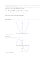
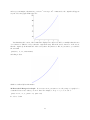
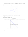
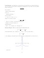
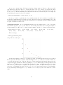
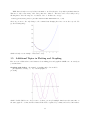
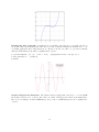
Let’s suppose you need to know the value of a root of
f (x) = x5 + x4 + x3 − x2 + x − 1
whose graph is
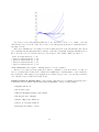
35
Furthermore, you are interested in a root between −1 and 1. This could come about because you graph
it (with or without SAGE), and see that there is a root in that region; or it could come about because you
see that f (−1) = −4 but f (1) = 2, and so clearly f crosses 0 at some point between −1 and 1, though we
don’t know where yet. Perhaps the problem in the textbook simply tells you that the root is between −1
and 1.
Okay, to solve the problem, you need only type this
find_root(x^5+x^4+x^3-x^2+x-1,-1,1)
and SAGE tells you that
0.71043425578721398
is the root. This is a numerical approximation, because quintic equations have a very special property—if
you don’t know what the special property is, just ask any math teacher.
While it is an approximation, the computer does several billion instructions per second, and so it is an
approximation that is trustworthy to around an accuracy of 10−16 , which is one tenth of a quadrillionth. So
it is a good approximation.
Meanwhile, it turns out there’s no root between −1 and 0. Perhaps you are told that, or perhaps you
graph it (with or without SAGE). If you type
find_root(x^5+x^4+x^3-x^2+x-1,-1,0)
then SAGE tells you
RuntimeError: f appears to have no zero on the interval
which is perfectly honest, because there’s no root in the interval for SAGE to go and find! If you have no
idea where the root is, you can type
find_root(x^5+x^4+x^3-x^2+x-1,-10^12,10^12)
which is asking SAGE to find a root that is between plus/minus one trillion.
Extremely sophisticated problems can be asked about. Some favorites of mine include if someone asks
you about xx = 5, then you could try to find where xx − 5 = 0. You would type
find_root(x^x-5,1,10)
or equivalently
find_root(x^x==5,1,10)
36
Another one is to find where ex = 1/x and you’d do that by finding a root of ex − 1/x = 0. You could
graph that with
plot( e^x - 1/x, -3, 3, ymin=-10, ymax=10)
obtaining the plot
and then you can see the root is between −1 and 1. This means that we should type
find_root(e^x-1/x,-1, 1)
will result in finding out that the root is at
0.56714329040979539
Last but not least, another favorite is to find sin x = cos x. It happens to be between 0 and π/2, which
you can see by graphing. The graph is
Now here you could ask for a root of (sin x) − (cos x). Alternatively, you can also type
find_root( cos(x) == sin(x), 0, pi/2 )
which is just easier notation.
37
Returning to an Old Problem Earlier, on Page 8, we saw a problem involving compound interest, and
finding how many months will be required to turn $ 5000 into $ 7000. Now let’s see how to solve that with
SAGE in only one line, rather than the previous approach which required the human to do some algebra.
The first line of our analysis was
7000 = 5000(1 + 0.045/12)n
and translating that into the language of SAGE results in
7000 == 5000*(1+0.045/12)^n
and so we should type
var(’n’)
find_root( 7000 == 5000*(1+0.045/12)^n, 0, 10000)
Note that the second line means that I’m searching for a value of n that makes the equation satisfied,
and that the value of n should be between 0 and 10,000. This seems reasonable, because 10,000 months is a
little over 833 years. The first line is just declaring n as a variable, which we saw on Page 31. In any case,
we get the answer 89.894060933080027 as before, and learn that 90 months will be required.
1.11
Using SAGE to take derivatives
The command for the derivative is just diff. For example, to take the derivative of f (x) = x3 − x you would
type:
diff( x^3 - x, x)
to learn the answer
3*x^2 - 1
Or for f (x) = sin(x2 ) you would type:
diff( sin(x^2), x )
to receive the answer
2*x*cos(x^2)
Sometimes you might have earlier defined your own function by
g(x)=e^(-10*x)
earlier, and so you can then type
diff(g(x), x)
to get the derivative, which is naturally
-10*e^(-10*x)
but you can also type
gprime(x) = diff(g, x)
38
which is silent, but then you can type gprime(2) or gprime(3) and it does what you expect. It tells you
the values of g 0 (2) and g 0 (3).
Another 100% equivalent form is
g(x).derivative()
SAGE can also do very difficult derivatives:
diff( x^x, x)
which provides the answer
(log(x) + 1)*x^x
Now if you’re interested in giving your calculus skills a workout, but possibly a very intense one, you can
try to see how you would calculate the derivative of xx with your pencil. In fact, if you happen to know
Newton’s Method, you can use that derivative and Newton’s Method to calculate the self-logarithm of a
number. Of course, many calculus teachers omit Newton’s Method, so do not feel bad if you haven’t been
taught it yet.
Plotting f (x) and f 0 (x) Together
One of my favorite bits of code in SAGE is
f(x)=x^3-x
fprime(x)=f(x).derivative()
plot( f(x), -2, 2, color=’blue’) + plot( fprime(x), -2, 2, color=’red’)
and I use this quite frequently. This plots f (x) and f 0 (x) on the same graph, with f (x) in blue, and f 0 (x)
in red. You can very easily change what function you are analyzing, but just changing that first line. Here
we are analyzing f (x) = x3 − x, in blue, and its derivative, f (x) = 3x2 − 1, in red. The plot is as follows:
Higher-Order Derivatives While you can find the second derivative by using diff twice, you can jump
directly to the second derivative with
diff( x^3-x, x, 2)
to get the answer
6*x
39
Third or higher derivatives are also no problem. For example, the third derivative can be found with
diff( x^3-x, x, 3)
For those who don’t mind typing more, you can do
derivative( x^3-x, x, 2)
which is more readable than writing diff.
1.12
Derivatives and Gradients in Multivariate Calculus
In the previous section, we learned about derivatives of single-variable functions. Now we’ll learn about
multivariate derivatives.
Partial Derivatives You’re probably not surprised to learn that SAGE can do partial derivatives very
easily. For example, if you have
g(x, y) = xy + sin(x2 ) + e−x
you can type
g(x,y) = x*y + sin(x^2) + e^(-x)
diff(g(x,y), x)
and get
2*x*cos(x^2) + y - e^(-x)
which is ∂g/∂x, and you can type
derivative(g(x,y), y)
to learn that ∂g/∂y is just x. Note here this really shows how diff and derivative are synonyms.
You can even find
∂2
f
∂x∂y
by typing derivative( g(x,y), x, y).
Gradients
If you want ∇f then you type
g.derivative()
and SAGE will correctly calculate the gradient. In fact, SAGE displays
(x, y) |--> (2*x*cos(x^2) + y - e^(-x), x)
which is to remind you that this is a map from a point (x, y) to a pair of real numbers, and not an
ordinary function. Interestingly, the gradient of a univariate function, done this way, is just the ordinary
first derivative, which is quite correct according to the laws of calculus.
An Extended Example: Marginal Cost in a Factory Coming Soon!
40
1.13
Using SAGE to calculate integrals, both numerically and
symbolically.
The only thing you need to understand in order to do integrals in SAGE is that there are really three
types of integrals that can be done: a numerical approximate integral, an exact definite integral, and an
indefinite integral. The first two types result in numbers, but which will be found approximately or exactly,
respectively. The third one is the antiderivative. If this is confusing, then let us consider a simple example:
Background: What integral might you want to consider, in order to find the area between the x-axis and
f (x) = x2 + 1 on the interval 3 ≤ x ≤ 6? Well, that integral would be
Z
6
2
x + 1 dx =
3
6 1 3
1 3
1 3
x +x =
6 +6 −
3 + 3 = 72 + 6 − 9 − 3 = 66
3
3
3
3
and that is a number. Here we’ve done it analytically, using calculus. This is an exact definite integral. It
is definite, because it ends with a number. It is exact, because we did no approximations.
On the other hand,
Z
1
x2 + 1 dx = x3 + x + C
3
is an indefinite integral. It produces a function, and not a number. Of course, we calculate an indefinite
integral on the way to calculating a definite one, but they are two distinct categories. If you want a function,
you should use the indefinite, and if you want a number, then you should use the definite.
Some integrals are famously impossible. The two most famous are the Fresnel
Z x
πt2
sin
dt
2
0
which is important in optics, and the Gaussian
Z
2
1
√ e(−x )/2
2π
which is pivotally important in probability. There is no function, built up of addition, subtraction, multiplication, division, roots, exponents, logarithms, trigonometric functions and inverse trigonometric functions
(as well as their hyperbolic cousins, which you might or might not have been taught about) which will have,
as its derivative, either the Fresnel or the Gaussian.
Yet, in applied mathematics, we need to calculate these integrals. In particular, the Gaussian is superbly
important in statistics. So what is done, is that the definite integral can be computed by dividing the interval
into many, many tiny regions. Lots of infinitesimal rectangles and trapezoids can be used to approximate
the curve. Each of these has a small amount of error, but when you add up all the areas, the hope is that
the area cancels out a bit. You probably did this during your calculus class at some point, or will at some
future point. Even more sophisticated methods include using polynomials instead of trapezoids, and SAGE
uses extraordinarily intricate techniques to make the best approximation possible. These approximations
are an old and deep subject, going back to Simpson’s Rule, where Simpson used tiny parabolas instead of
trapezoids.
The above might have been a bit confusing, but the whole point of SAGE is that it will worry about these
details for you, so long as you know what you want from SAGE. I hope this background was interesting and
at least partially clear. If not, you should probably discuss it with your calculus instructor, before proceeding
further.
41
The Indefinite Integral: The indefinite integral is the simplest, and for example if you wanted to know
Z
x sin(x2 )dx
you would simply type
integral( x*sin(x^2), x )
and then you’d learn the answer is
-1/2*cos(x^2)
Similarly, if you wanted to know
Z
x2
x
dx
+1
you would simply type
integral( x/(x^2 + 1), x )
and then you’d learn the answer is
1/2*log(x^2 + 1)
The Definite Integral: Alternatively, we could put a lower bound of 0 and an upper bound of 1 on that
integral, and then get
Z 1
x
dx
2+1
x
0
becomes
integral( x/(x^2 + 1), x, 0, 1 )
and so we discover
1/2*log(2)
is the answer, but remember that “log” means the natural logarithm, not the common logarithm.
More Difficult Cases: Consider the following function f
3
f (x) = e−x sin(x2 )
which is a nice continuous function. We can find its plot with
plot( exp( -x^3 ) * sin(x^2), -5, 5, ymin = 0, ymax=1 )
which yields the plot:
42
The function is interesting, but the integral is quite frustrating. I cannot solve that integral with my
pencil, and I am willing to wager that you cannot either. Try it if you like.
While it is the case that there is some function, somewhere, which has f as its derivative, which is a
logical consequence of some advanced real analysis and the fact that f is continuous, the practicalities of
the matter are that there is no way to write the integral. To be really precise, there is no function, built up
of addition, subtraction, multiplication, division, roots, exponents, logarithms, trigonometric functions and
inverse trigonometric functions (as well as their hyperbolic cousins, which you might or might not have been
taught about) which will have, as its derivative,
In other words f is integrable, but the integral cannot be written in terms of common (and not so
common) functions.
Thus since
Z
3
e−x sin(x2 )dx
does not have a nice expression, then when you type
integral( exp(-x^3)*sin(x^2),x)
the SAGE replies not with an answer, but instead with
integrate(e^(-x^3)*sin(x^2), x)
which represents an admission of defeat. Have no fear, however, because we can calculate numerical answers
approximately, with very high accuracy, and we’ll learn about that momentarily.
A nefarious integral, famous among calculus teachers, is
Z
t20 et dt
where the 20 could be any decently large number. This comes up in explaining what Euler’s gamma function
is, but we aren’t too concerned with that right now. In any case, we could just type
integral( (t^20)*(e^t), t )
but then we get back
(t^20 - 20*t^19 + 380*t^18 - 6840*t^17 + 116280*t^16 - 1860480*t^15 + 27907200*t^14
- 390700800*t^13 + 5079110400*t^12 - 60949324800*t^11 + 670442572800*t^10 6704425728000*t^9 + 60339831552000*t^8 - 482718652416000*t^7 +
3379030566912000*t^6 - 20274183401472000*t^5 + 101370917007360000*t^4
- 405483668029440000*t^3 + 1216451004088320000*t^2 - 2432902008176640000*t
+ 2432902008176640000)*e^t
which is large enough that it isn’t clear how to get an idea of what that means. If instead, we had certain
bounds, such as to calculate
Z 3
t20 et dt
2
then we would type
integral( (t^20)*(e^t), t, 2, 3 )
and get instead
-329257482363600896*e^2 + 121127059051462881*e^3
which is getting toward an answer! On the other hand, if you really want a numerical answer then you
should use our old friend n() and type
43
n( integral( (t^20)*(e^t), t, 2, 3 ) )
which would return the number
8.79797452800000e9
and that means 8.79797452800000 × 109 . This highlights the difference and similarities of the various types
of answer.
A Theoretical Side Note: That number which we just calculated looks like an integer, because it ends
with 528 when you carry out the 109 part—but when we look at the exact answer, we can see that no, it is
not an integer, because e2 and e3 are involved, and e is an irrational number. It is quite possible that you
haven’t yet learned what irrational numbers are, but if not, then ask any math teacher They will be happy
to discuss such an advanced topic with you. Whenever dealing with computations, it is critical to remember
what is an approximation, and what is exact. Irrational number can be expressed exactly on occasion (like
we just did here, using e2 and e3 ) but that is the exception and not the rule. In any case, this paragraph
has nothing to do with SAGE, and so we return to the topic at hand.
Numerical Integrals: Speaking of approximations, you can also jump to the numerical integral very
rapidly. I’m sure we can both calculate
Z
1
3
x − x dx =
0
1 1 4 1 2
1 4 1 2
1 1
1
1 4 1 2 x − x =
1 − 1 −
0 − 0 = − =−
4
2
4
2
4
2
4
2
4
0
but if you wanted to ask SAGE to calculate this numerically, then you should type
numerical_integral( x^3 - x, 0, 1)
which would output
(-0.24999999999999997, 2.775557561562891e-15)
where the first number is the best guess SAGE has for the answer, while the second number is the uncertainty.
In this case, the uncertainty is 2.77 quadrillionths—which is very impressive.
Of course, SAGE can do this integral exactly as well, using the commands we learned moments ago.
What is interesting about numerical integration, are the cases when you cannot do the indefinite integral,
because like the Fresnel above it cannot be written, but you can find good numerical estimates. Consider
again
Z
3
3
e−x sin(x2 )dx
1
but now with bounds, so that it can be done numerically. We would type
numerical_integral( exp(-x^3)*sin(x^2),1,3)
and that returns back
(0.077997011262087815, 8.6840496851995037e-16)
with (as before) the first number being the answer, and the second the accuracy. In this case, the uncertainty
is 868 quintillionths—which is very impressive. Another way to say it is that the uncertainty is (1/1152)
trillionths.
44
Partial Fractions One thing that is very important in problems that arise from Differential Equations
and even Calculus II is the question of integration by partial fractions. If you want to know the partial
fraction break-down of
x3 − x
x2 + 5x + 6
then you must do
f(x)=(x^3-x)/(x^2+5*x+6)
followed by
f.partial_fraction()
and get the answer
x - 6/(x + 2) + 24/(x + 3) - 5
which is correct. In fact, it means
24
6
+
−5
x+2 x+3
However, you can also do the shortcut and ask instead
x−
integral( (x^3-x)/(x^2+5*x+6), x )
which will result in
1/2*x^2 - 5*x - 6*log(x + 2) + 24*log(x + 3)
Improper Integrals
While the following integral is mathematically valid
Z
1
1
−1 + 2 dx = −x − + C
x
x
and the right-hand side can be evaluated at x = −1 and x = 1, there is no finite answer to
Z −1
1
−1 + 2 dx
x
−1
because this improper integral is divergent. The graph will reveal why that is the case. Here is the plot,
generated by
45
plot( -1+1/x^2, -10, 10, ymin=-2, ymax=2 )
Yet, SAGE knows this and will say
-x - 1/x
in response to
integral(-1+1/x^2,x)
but instead will respond
ValueError: Integral is divergent.
to the inquiry
integral(-1+1/x^2,x,-1,1)
Another type of improper integral is
Z
∞
2
1
dx
x2
and the way to write that in SAGE is to type
integral(1/x^2,x,2,oo)
to which SAGE responds 1/2, or another example is
Z ∞
2
e−x dx
−∞
which in SAGE is
integral(exp(-x^2),x,-oo,oo)
√
and it gives the correct response of π.
The idea is simply that oo is a special code for “infinity.” It is two letter o’s, and the idea is that if you
squint, it looks like an infinity symbol.
The Function erf and Integrals:
Among mathematicians and especially among statisticians, the integral
Z y
2
2
√ e(−x ) dx = erf(y)
π
0
which is just a slight variant of the one that I told you earlier cannot be found using the elementary functions
of mathematics, is so important that they gave it a name, and that name is erf. While being friendly and
pronounceable, erf stands for the “Error Function.”
Thus if you type into SAGE
integral( (2/sqrt(pi)) * exp(-x^2), x, -oo, 2)
it will respond
(sqrt(pi)*erf(2) + sqrt(pi))/sqrt(pi)
46
which is correct because
Z
2
−∞
2
2
√ e(−x ) dx =
π
Z
0
−∞
2
2
√ e(−x ) dx +
π
Z
0
2
√
√
√
π
π + πerf(2)
2 (−x2 )
√ e
√
dx = 1 + erf(2) = √ (1 + erf(2)) =
π
π
π
Perhaps you might find that 1 + erf(2) is a more compact and simpler answer. I would be inclined to
agree. I’m not quite sure why SAGE does not simply its final answer further.
In any case, the point is that there are some functions out there which do not have integrals writable
using elementary functions, but, which SAGE calculates anyway, using the erf function. Not all calculus
textbooks are anticipating that, and there can be some unexpected surprises when you compute an answer
to a textbook problem, and look in the back of the book, only to find that your textbook tells you that the
problem is unsolvable. It really is a matter of whether or not you accept erf as a legitimate or illegitimate
member of the family of functions.
1.14
Matrices in SAGE, Part Two
Coming Soon!
This will include using SAGE to multiply and invert matrices, and take determinants, as well as adding
and subtracting matrices. Also the backslash operator.
Meanwhile, here is a command list, if you need to look up the commands:
• The two ways to declare a matrix.
• vector
• augment
• A.solve right(v)
• A.solve left(v)
• A.echelon form()
• A.rref()
• A.inverse()
• The backslash operator
• Matrix Multiplication
• The identity matrix
• det(A)
47
Chapter 2
Fun Exploration Projects using SAGE
Here are some extended examples of using SAGE to explore a non-trivial problem in an area outside of
computer algebra. We present one example from each of several disciplines. All of these projects can be
explored using information taught in Chapter One, and do not require any additional familiarity with SAGE.
Pure Mathematics Analyzing a quintic polynomial’s features, for graphing.
Finance Analyzing a mortgage.
Physics Measuring the effect of gravity on a space satellite.
Microeconomics Modeling the effect of the selling price on the sales of ice cream.
Engineering Exploring the effects of a two-stage rocket where the first stage fails to detach.
Ecology Approximating the impact of toxic waste on the oxygen content of a large lake.
Astronomy Finding the point of closest approach of a comet to the orbit of the earth.
Earth Sciences Discovering the relationship between the time of sunrise and sunset, with latitude and
time of year.
Medicine Modeling the flow of blood in an artery.
Business Calculating the optimal array of vehicles in a corporation’s fleet for transporting gasoline.
Biology Modeling the interactions between two species—one a predator; the other, prey.
The examples for “physics” and “finance” as well as “microeconomics” are fully written and are included
here. I have used the examples for “engineering” and “business” in class as projects, but need to convert
those PDFs into LaTeX for inclusion in the book. The “pure mathematics” example is available as a Sage
worksheet, but needs conversion into LaTeX.
The “ecology” example was done in a lecture of mine, so it might require a bit of time to convert into
a project, but not much. The “astronomy” example was an exam question of mine, so that might require a
bit more time. The “earth sciences,” “medicine,” and “biology” examples have not been written yet.
2.1
The Pure Math Example: Quintics
Coming Soon! Given a quintic polynomial, trying to find the correct window for graphing, by Prof. Ben
Jones. I hope to write this soon, but until I do, you can find it at:
https://sage.uwstout.edu:8000/home/pub/21
and https://sage.uwstout.edu:8000/home/pub/23
48
2.2
The Finance Example: Mortgages
This example assumes you know how to do mortgage calculations. If you don’t, then you might want to
read a different example.
Let us say that you want to sell some mortgage products, and you want to compute the cost-per-thousand
for several loans at interest rate r and compounded monthly. If the length is for t years, then the number of
compoundings is n = mt = 12t. The interest-rate-per-compounding-period would be i = r/m = r/12 and
value would be V = 1000. So we would start with the basic formula
Vi
1 − (1 + i)−n
and plug in all that data. Since V = 1000 is not going to change, we can assign that one with
PMT =
V=1000
to make it a long term constant. Note, SAGE accepts your constant quietly, it does not give a response.
Then, we could define our own function, as described earlier
CostPerThousand (i, n) = ( V * i ) / (1 - (1+i)^(-n) )
and so for a 30 year mortgage at 6.5% compounded monthly, we can do
CostPerThousand ( 0.065/12, 30*12)
and then if the rate rises to 7% we can do
CostPerThousand ( 0.07/12, 30*12)
and so on, and so forth.
Notice that the function name has to be only one word, but by varying the capitalization that way (which
programmers call “Camel Case”), we could express an idea that was more than one word. Surely it is much
easier to read CostPerThousand than costperthousand or COSTPERTHOUSAND.
While this above function is nice, (for example it will save us from agonizing each time over the placement
of the parentheses,) it also isn’t quite perfect. Our data will be given in terms of the number of years of the
loan t, not the number of payments n = mt = 12t. Likewise, the rate will be the nominal, published rate r
not the per-period rate i = r/m = r/12. One student once described this to me by saying that the n and i
are math-friendly, whereas the t and r are human-friendly.
This can be fixed by doing
CostPerThousand1 (r, t)=CostPerThousand( i=r/12, n=12*t )
and now we have made a new formula, which uses the rate in terms of r as we liked, and the number of years
t, not the number of compounding periods. And now, for a 30 year mortgage at 6.5% compounded monthly,
we can do
CostPerThousand1 ( 0.065, 30)
and get a more user-friendly input and output.
The Grouping Symbols: Just a reminder, while a mathematician might write
P V = P M T [1 − (1 + i)−n ]/i
for the present value formula, using the [ and ] as a sort of auxiliary ( and ), in SAGE, the only grouping
operators are parentheses. So that formula is
PV = PMT * (1 - (1+i)^(-n))/i
with additional explanation found on Page 5.
49
2.3
The Physics Example: Gravitation and Satellites
Let’s say you’re analyzing a satellite in its orbit around the earth. Newton’s formula for gravity is
F =
GMe Ms
rs2
where G = 6.77 × 10−11 N m2 /kg 2 is the universal constant for gravitation; Me = 5.9742 × 1024 kg is the
mass of the earth; next rs is the distance from the satellite to the center of the earth in meters; and finally
Ms kg is the mass of the satellite. Surely G and Me will not change, so we can set those with
G = 6.77 * 10^(-11)
Me = 5.9742 * 10^(24)
just like we set c = 355/113 on Page 23.
Unlike the mass of the earth, or the universal constant of gravitation, the distance to the satellite might
change quite often, and the mass of the satellite could change also (particularly if it has fuel aboard, which
will be burned during maneuvers). So for those, we should make a function
Force( Ms, rs ) = (G * Me * Ms)/(rs^2)
and you could do things like
Force( 1000, 10 * 10^6 )
to get answers. This is great if you have a large number of points that you’re interested in, and want to save
a lot of typing.
Suppose now that you really wanted the function to work in terms of altitude, as measured from the
earth’s surface, and not from the center of the earth. Well it is easy to realize that you just have to add the
radius of the earth. First, you put in the radius of the earth, which is 6378.1 km, but of course we should
switch it to meters to avoid unit conflicts.
re = 6378100
Then you can define
Force1( Ms, alt ) = Force( Ms, alt + re )
and then you can just go ahead and use Force1. For example,
Force1( 1000, 3621900 )
is roughly equivalent to what we had before. I suppose it depends upon if the problem you are given is in
terms of altitude, or distance from the center of the earth.
This idea of building functions on top of functions is very powerful. I have often written large suites
of functions in this way—one function on top of the other function, on top of the next—to model complex
phenomena in SAGE.
50
2.4
The Microeconomic Example: Selling Price
Once I was told that the goal of the first microeconomics course should be twofold. First, to teach the
concept of “supply and demand.” Second, to teach that the three actions of “maximizing profit,” versus
“maximizing revenue,” or “minimizing costs,” are three extremely different things.
This example will look at that second objective. Here is an extended study of the micro-economics of
the sale of ice cream. We imagine a vendor with an ice-cream cart at a busy intersection in Central Park.
An ice cream salesman observes that when he charges $ 3 per ice cream, he only sells 120 cones per day.
On the other hand, when he charges $ 2 per ice cream, he sells 200 cones per day. If he makes his price to
high, he will sell too few, and won’t make much profit. If he makes his price too low, he will sell more, but
he still won’t make much profit. The costs of doing business are basically just 50 cents per cone, because he
has long since paid off his start-up expenses, plus a $ 100 fee per day for the rental of the ice cream cart.
The ice cream salesman is going to assume that the demand varies linearly with price. This often is not
quite true, but it is often a reasonable approximation. There are several different ways to realize that the
demand n, and the price p, will have the relationship
n = 360 − 80p
or equivalently
p = 4.50 − n/80
and you can check that by plugging-in the given data points. The easy way to find that equation is to
compute the slope connecting the points (200, 2) and (120, 3), and then find the equation of the line between
those two points.
Let’s pause a moment, and see if this makes sense. First, plugging in n = 200 and n = 120, we do get
the prices of $ 2 and $ 3 that we expect. If we set p = 2.50, then we get 160, as we would anticipate—that’s
the midpoint. At a price of $ 4.50, then we sell no ice cream. This could be believable, if people are usually
expecting to pay around $ 2, then you cannot charge them more than double what they are accustomed
to pay. If the price is $ 0, then we sell 360 cones per day—that’s called the saturation point and that’s
a lot of ice cream. The model breaks down for prices over $ 4.50, because it predicts a sale of a negative
number of cones, which does not make sense. Likewise, if you set a demand above 360 cones per day (the
“saturation point”) then a negative price is called for, which also does not make sense. So the model is valid
for 0 ≤ p ≤ 4.50, or equivalently 0 ≤ n ≤ 360 cones.
Clearly if one sells n cones at price p, then the revenue is np. So then we have
r(n) = np = 4.50n − (n2 )/80
as the revenue function. Meanwhile, the cost function is 50 cents per cone, plus $ 100, for a total of
c(n) = 0.50n + 100
and that gives us a profit function of
−n2
+ 4n − 100
80
which is a parabola. It makes sense that we should get some sort of curve, because if you make the price
very low, or very high, then the profit is zero or worse—you have a loss. Somewhere in the middle is the
sweet spot.
Before we graph this, if you are inexperienced in this kind of analysis, let’s make a table and see that it
makes sense and matches our prior data:
p(n) =
51
Price Cones Sold Revenue Costs
Profit
0.00
360
0.00
280.00 -280.00
0.50
320
160.00
260.00 -100.00
1.00
280
280.00
240.00 40.00
1.50
240
360.00
220.00 140.00
2.00
200
400.00
200.00 200.00
2.50
160
400.00
180.00 220.00
3.00
120
360.00
160.00 200.00
3.50
80
280.00
140.00 140.00
4.00
40
160.00
120.00 40.00
4.50
0
0.00
100.00 -100.00
I recommend that you pick 2 or 3 values, and manually verify those 2 or 3 rows of the table, before
continuing onward.
Okay, did you really verify 2 or 3 rows of the above? It is really useful to do so before reading further.
In any case, here’s the graph
where you can see that the revenue function is in black, the cost function is in red, and the profit function
is in green. There are lots of facts that can be gleaned from this:
• When red cross black, that means that cost and revenue cross each other, that’s the break-even point.
Here we have two break even points, one just under 30, and one just under 300. Let’s find them. We
would type
find_root((-x^2)/80 + 4.5*x == 0.5*x+100, 250, 350)
and also
find_root((-x^2)/80 + 4.5*x == 0.5*x+100, 10, 50)
to find out that at roughly 292.664 cones and 27.3350 cones, we break even. Between these values is a
profit, and outside these values, there is a loss. That seems to match the data in the table.
• The other definition of the break-even point is when profit is zero. So we could have typed
find_root((-x^2)/80 + 4*x - 100, 10, 50)
and also
52
find_root((-x^2)/80 + 4*x - 100, 250, 350)
to find those same values (292.664 and 27.3350), and you’ll see that the green curve crosses the x-axis
there.
• The cost function is never zero. That’s because the salesman has to pay the $ 100 per day fee.
• The revenue function is zero at two points. First, when no ice cream is sold—that makes sense. We
found earlier that is at $ 4.50 per cone, and 0 cones per day. Second, revenue is zero when the ice
cream is sold for 0 cents per cone. Clearly, if you don’t charge anything, then there is no revenue.
That occurs at the saturation point, of 360 cones per day and $ 0 per cone. In SAGE, we would type
find_root( 4.50*x-(x^2)/80, 0, 50)
and also
find_root( 4.50*x-(x^2)/80, 300, 400)
to get the values 0.0 and 360.0.
• Now we’ve found when profit is zero and when revenue is zero, and determined that cost is never zero.
The next step is to try to minimize or maximize these functions. If you’ve had calculus, then you know
how to minimize or maximize a polynomial. If not, then you might recall the fact that a parabola
y = ax2 + bx + c has its optimum at the point x = −b/2a.
• For the revenue function, we see that maximum revenue occurs at 180 cones, a cost of $ 2.25 per cone,
and a revenue of $ 405. The costs would be $ 190, for a profit of $ 215.
• For the profit function, we see that maximum profit occurs at 160 cones, a cost of $ 2.50 per cone, and
a revenue of $ 400. The costs would be $ 180, for a profit of $ 220.
• The point of minimum costs would be 0 cones of ice cream, for a cost of $ 100. However, the revenue
is $ 0 and the profit is negative, a loss of $ 100. Definitely, this is not a good business plan. (Even if
the costs are lower in this bullet than in the previous two bullets.)
• Did you notice how the point of maximum profit had lower revenue (400 vs 405) but higher profit (220
vs 215) than the point of maximum revenue? Did you notice how the point of maximum revenue had
lower profit (215 vs 220) but higher revenue (405 vs 400) than the point of maximum profit?
In conclusion, we see that “maximizing revenue,” “minimizing costs,” and “maximizing profit,” are three
different objectives.
2.5
The Engineering Example: Two-Stage Rockets
Coming soon!
2.6
The Ecology Example: Lake Dumping
Coming soon!
2.7
The Astronomy Example: Point of Closest Approach
Coming soon!
53
2.8
The Earth Science Example: Sunrise and Sunset
Coming soon!
2.9
The Medical Example: Blood in an Artery
Coming soon!
2.10
The Business Example: a Vehicle Fleet
Coming soon!
2.11
The Biology Example: Predator/Prey Models
Coming soon!
54
Chapter 3
Advanced Features of SAGE
3.1
Using SAGE to work with integers. (gcd, lcm, factorization,
sigma, tau, etc. . . )
The study of problems that deal with the integers, in pure mathematics, is called “number theory”, and in
certain types of applied mathematics, called “integer programming.” This subject can be started at a very
young age (e.g. “what is a prime number?”) but can be very advanced too. Many Ph.D. dissertations are
written every year with new results in number theory. Mostly, number theory is about writing proofs, and
so you’d imagine that SAGE is not very useful for that. Actually, SAGE is very good at working with the
integers to help you work out specific examples on what the instruments of number theory do to specific
integers. This can help you understand new concepts more intimately, and I find it can form a bridge between
the lecture on a topic and the time when you are really ready to write serious proofs about a topic.
For example, you can type factor(-2007) to find the factorization of that integer, which is
-1 * 3^2 * 223
and likewise
factor(2008)
is
2^3 * 251
To find the next prime number after one million, you can do
next_prime( 10^6 )
and discover the answer is 1,000,003.
You can also test a number for primality. Consider is prime(101) or alternatively is prime(102) .
Of course, SAGE says True for 101, and False for 102.
Last but not least, you can find all the primes in a certain interval. For example
prime_range(1000,1100)
gives you all the prime numbers between 1000 and 1100.
55
The gcd and the lcm
120 and 64, just type
To find the “greatest common denominator” or “gcd” of two numbers, perhaps
gcd ( 120, 64 )
and you will learn that the answer is 8. This makes sense because 120/8 = 15 while 64/8 = 8, and as you can
see, 15 and 8 share no common factors. More explicitly, we can look at the prime factorizations 15 = 5 × 3
and 8 = 2 × 2 × 2. Another way of looking at that is
120 = 23 × 3 × 5 while 64 = 26
and so all that 120 and 64 have in common is just 23 , which is 8.
Likewise, you can find the “least common multiple” or lcm. This is done by typing
lcm( 120, 64 )
from which you learn that the lcm is 960. This makes sense because 960/120 = 8 and also 960/64 = 15,
and again 8 shares no factors with 15. A mathematician would say “8 is coprime to 15.” Some authors say
“mutually prime” instead of “coprime.”
Another way to look at it is that the lcm should be
26 × 31 × 51 = 960
because the 2 appears 6 times in 64 and 3 times in 120 (thus a maximum of 6), while the 3 and 5 both
appear 0 times in 64 and 1 time in 120 (thus a maximum of 1 each). Raising each of those primes (2, 3, and
5) to those powers (6, 1, and 1) gives the lcm.
Before we continue, one more example is helpful. Let’s work with slightly larger numbers, perhaps 3600
and 1000. First, we do the prime factorizations
3600 = 24 × 32 × 52 while 1000 = 23 × 53
and we can compute the lcm by taking the maximum exponent each time
24 × 32 × 53 = 18, 000
and the gcd by taking the minimum exponent each time
23 × 30 × 52 = 200
Take a moment to verify that 200 goes into both 1000 and 3600, as well as the fact that no higher number
will. Next, take another moment to verify that both 1000 and 3600 go into 18,000, but there is no lower
number for which that’s true. And of course, the product of the numbers divided by the gcd is the lcm, and
the product of the numbers divided by the lcm is the gcd.
The key here is to realize that the prime factorization of a number communicates an enormous amount
of information about that number.
Several gcds or lcms at Once If you want to take the gcd of many numbers at once (for example 120,
55, 25, and 35), there’s no need to do
gcd( 120, gcd(55, gcd(25, 35 ) ) )
because you can do instead
gcd( [ 120, 55, 25, 35 ] )
to get 5 and likewise
56
lcm( [ 120, 55, 25, 35 ] )
to get 46,200. This is another example of a list in SAGE. You can enclose any data with [ and ], and
separate the entries with commas, to make a list. We saw this in graphing multiple functions at once, on
Page 68, and in solving equations exactly, on Page 32. We’ll see this again in scatter plotting live data, on
Page 62.
And you can even verify the theorem that says the product of all the numbers in the list, divided by their
gcd raised to the power of one less than the length of the list, equals the lcm. Since we have four numbers
in our list, we would divide by the cube of the gcd. This is done by
120*55*25*35 / 5^3
More about Prime Numbers One neat trick is that if you wanted to find the 54,321th prime number,
you could type
nth_prime(54321)
and discover that it is 670177. You can double check this with
factor(670177)
which returns itself, confirming that the number is prime.
Phi Sometimes it is useful to know how many integers are coprime to x, from the range 1 to x. For
example, how many numbers from 1 to 100 share a factor with 10, and how many are coprime with 10. Well,
the prime factors of 100 are 2 and 5, and so any number composed only of twos and fives will work. This
would be
{2, 4, 5, 6, 8, 10}
and so the other numbers
{1, 3, 7, 9}
are coprime with 10. In particular, if you know what modular arithmetic is, then these are the numbers that
have “multiplicative inverses” or “reciprocals” mod 10. Since 4 numbers are coprime to 10, we will write
φ(10) = 4.
Even if you don’t know what modular arithmetic is, consider 7. Each of
{1, 2, 3, 4, 5, 6}
is coprime to 7, because the only prime that divides 7 is 7, and 7 does not divide any of those. So, 6 out of
the 6 numbers are coprime to 7, and we would then write φ(7) = 6. It will always be the case for a prime
number that φ(p) = p − 1. On the other hand, consider 12. Then among
{1, 2, 3, 4, 5, 6, 7, 8, 9, 10, 11}
we see that both 2 and 12 are divisible by 2; both 3 and 12 are divisible by 3; both 4 and 12 are divisible by
2; both 6 and 12 are divisible by either 2 or 3; both 8 and 12 are divisible by 2; both 9 and 12 are divisible
by 3; both 10 and 12 are divisible by 5. Finally, this means that only 1, 5, 7, and 11 are coprime to 12, and
so φ(12) = 4.
It would be very annoying to calculate φ of a 100-digit number, such as when working with cryptography,
the science of codes. All you need to do in SAGE is type
euler_phi(12)
and then you learn that the answer is 4. It is called “euler phi” because it was discovered by Leonhard
Euler.
57
The Divisors of a Number Meanwhile, consider the set of divisors of a number. If you want to know
the set of divisors of 12, which means the set of positive integers dividing 12, you would type
divisors(12)
and get then
[1, 2, 5, 10, 25, 50, 125, 250]
and likewise
divisors(312500)
gives you
[1, 2, 4, 5, 10, 20, 25, 50, 100, 125, 250, 500, 625, 1250, 2500,
3125, 6250, 12500, 15625, 31250, 62500, 78125, 156250, 312500]
but remember, it is very important to not have any commas separating the thousands, when inputting large
numbers into SAGE.
Sometimes in number theory, we want to calculate the sums of the squares or cubes of the divisors. I
can’t think of an example why at the moment, but I’m sure there’s a good one. Consider that 45 has as its
divisors {1, 3, 5, 9, 15, 45}. Then we have sigma coming to 78, because
1 + 3 + 5 + 9 + 15 + 45 = 78
and then the sum of squares would be
12 + 32 + 52 + 92 + 152 + 452 = 2366
and with cubes
13 + 33 + 53 + 93 + 153 + 453 = 95, 382
but in SAGE the commands for that are
sigma( 45, 2 )
for squares and
sigma( 45, 3 )
for cubes.
Likewise
sigma( 45, 1 )
is the same as sigma.
Now there’s a fun game that the Arabs used to play in the Medieval Period. Consider two particular
numbers 220 and 284. The divisors are
divisors(220) = {1, 2, 4, 5, 10, 11, 20, 22, 44, 55, 110, 220}
and then they would calculate
1 + 2 + 4 + 5 + 10 + 11 + 20 + 22 + 44 + 55 + 110 = 284
but on the other hand
divisors(284) = {1, 2, 4, 71, 142, 284}
which yields
1 + 2 + 4 + 71 + 142 + 284 = 220
and so we see 220 and 284 are intimately related.
The Arabs found this so moving that they inscribed these numbers on jewelry that they would give to
their spouses and so forth. These are called Amicable Pairs—220 representing the young lady, and 284
representing the young gentleman. You can find this in SAGE via
58
sigma( 220 )-220
and
sigma( 284 )-284
Tau As you know, some fractions like 1/4 and 1/2 as well as 1/25 can be expressed as decimal fractions
which terminate. Others, like 1/3 or 1/9 will repeat. It is pretty easy to see why a fraction can be expressed
as an exact terminating decimal fraction of n decimal places (or fewer) if and only if the denominator divides
10n . Take a moment to convince yourself of this, or alternatively, consider the following example. If we want
to know what denominators result in a two-decimal place (or fewer) exact terminating decimal, we would
just need to see what positive integers divide 100. In SAGE we’d do
divisors(100)
and then get
[1, 2, 4, 5, 10, 20, 25, 50, 100]
but in binary, the analogous rule would be 2n . It is obvious that the only positive integers which divide
2n are the numbers 1, 2, 4, 8, . . . , 2n . Therefore, we can use this criterion for seeing which number bases are
convenient for fractions, and which are not.
Now, we’ll consider the Babylonian numbering system which is base 60. Two symbols would be sufficient
to describe any fraction with the following denominators:
[1, 2, 3, 4, 5, 6, 8, 9, 10, 12, 15, 16, 18, 20, 24, 25, 30, 36,
40, 45, 48, 50, 60, 72, 75, 80, 90, 100, 120, 144, 150, 180, 200, 225, 240,
300, 360, 400, 450, 600, 720, 900, 1200, 1800, 3600]
Did you notice how in decimal, there were 9 denominators, but in base 60, there were 45 denominators?
Or if you do not count one, then 8 versus 44? What we really wanted to do was count the divisors. The
function for counting the number of (positive integer) divisors of an integer is τ , and in SAGE is given by
sigma(3600, 0)
which just tabulates 1 for each divisor. In other words, each divisor is raised to the 0th power, thus becomes
1, and then if you add those up, you learn how many divisors there are.
Modular Arithmetic:
To find out what 1939 is mod 37, you can type
1939 % 37
but the % operator takes the modular reduction only of the nearest number. This means that to evalulate
(32 )4 + 2 mod 5
you must not type
3^2*4 + 2%5
which evaluates to 38, but rather
(3^2*4 + 2) %5
59
which gives 3, the correct residue.
The opposite of the “mod” operator is the integer quotient. To find the integer quotient of a number,
use
25 // 4
to get 6. This is the quotient rounded down to the nearest integer.
You can define
def is_even(n): return n%2 == 0
which will return True for even integers, and False for odd ones. This can then be used to wrap up into
other if statements. We’ll talk much more about if statements in the chapter on programming.
3.2
Minor Commands of SAGE
Here we list a few commands
that require them.
min(x,y)
max(x,y)
floor(x)
ceil(x)
factorial(n)
that come up from time to time. They can be quite useful in the situations
Returns either x or y, whichever is smaller.
Returns either x or y, whichever is greater.
Just round x down, or bxc
Just round x up, or dxe
This is n!, also called “n factorial.”
binomial(x,m)
This is usually written
x
m
binomial(x,m) * m!
This is usually written
x!
m!
3.2.1
or
x!
m!(x−m)!
or x Cm
or x Pm
Rounding, Floors, and Ceilings
As you can see, the floor command rounds a number down, and the ceil command rounds a number up.
In older books, the “floor” function is sometimes called “The Greatest Integer Function.” This is because
it can be defined by “the greatest integer that is less than or equal to x.” Some older mathematics books
will write [x] instead of bxc. I suppose if you wanted, you could define the ceiling function by “the least
integer that is greater than or equal to x.”
3.2.2
Combinations and Permutations
In a lot of textbooks, particularly for Finite Mathematics, or Quantitative Literacy, as well as a basic
Probability & Statistics, a lot of time is spend talking about combinations and permutations. For example,
if I have 52 distinct cards in a deck of cards, I might ask how many 5-card hands I can build with them.
If order doesn’t matter, such as in Poker, then I would have
52
52!
52 × 51 × 50 × 49 × 48
=
=
= a lot
52 C5 =
5
5!47!
5×4×3×2×1
possibilities, and SAGE calls this binomial(52, 5). This is an example of the “combinations” formula.
However, if order does matter, which is not the case for poker, then I would have
52
52!
= 52 × 51 × 50 × 49 × 48 = even more
P
=
5! =
52 5
5
47!
possibilities. In SAGE, you can type
factorial(52)/factorial(52-5)
60
for that, or you can type
binomial(52,5)*factorial(5)
both of which return the same answer. This is an example of the “permutations” formula.
You might be wondering why SAGE does not have a command for permutations, but that it does have
a command for combinations. Well, there is a command for permutations, but it does something a bit more
than the above. In the above work, we calculated how many permutations, but sometimes you might want
to know what those permutations are. For this you can type
myset=[’ace’, ’king’, ’queen’, ’jack’]
permutations(myset)
and it will obediently display all 24 possibilities:
[[’ace’, ’king’, ’queen’, ’jack’], [’ace’, ’king’, ’jack’, ’queen’],
[’ace’, ’queen’, ’king’, ’jack’], [’ace’, ’queen’, ’jack’, ’king’],
[’ace’, ’jack’, ’king’, ’queen’], [’ace’, ’jack’, ’queen’, ’king’],
[’king’, ’ace’, ’queen’, ’jack’], [’king’, ’ace’, ’jack’, ’queen’],
[’king’, ’queen’, ’ace’, ’jack’], [’king’, ’queen’, ’jack’, ’ace’],
[’king’, ’jack’, ’ace’, ’queen’], [’king’, ’jack’, ’queen’, ’ace’],
[’queen’, ’ace’, ’king’, ’jack’], [’queen’, ’ace’, ’jack’, ’king’],
[’queen’, ’king’, ’ace’, ’jack’], [’queen’, ’king’, ’jack’, ’ace’],
[’queen’, ’jack’, ’ace’, ’king’], [’queen’, ’jack’, ’king’, ’ace’],
[’jack’, ’ace’, ’king’, ’queen’], [’jack’, ’ace’, ’queen’, ’king’],
[’jack’, ’king’, ’ace’, ’queen’], [’jack’, ’king’, ’queen’, ’ace’],
[’jack’, ’queen’, ’ace’, ’king’], [’jack’, ’queen’, ’king’, ’ace’]]
Try instead
myset=[’ace’, ’king’, ’queen’, ’jack’, ’ten’]
permutations(myset)
if you are curious.
3.2.3
Calculating Limits Expressly
If you wanted to calculate
lim
x→0
x−2
x−3
you should type
limit( (x-2)/(x-3), x=0)
to learn that the answer is 2/3, which is perhaps obvious. Perhaps less obvious would be the limit
x2 − 4x + 3
x→1 x2 − 3x + 2
lim
for which you should type
limit( (x^2-4*x+3)/(x^2-3*x+2), x=1)
61
to obtain the answer “2.” If you do not know how to do that without a computer or calculator (in other
words, only with pen and pencil), then let me suggest that you try factoring those two polynomials as a first
step.
Last but not least, if you wanted to verify the strange and amazing fact
lim (cos x)
1/x2
x→0
1
=√
e
then you should type
limit( cos(x)^(1/x^2), x=0)
to obtain the desired answer
e^(-1/2)
To show that the last limit there, given in terms of cosine and x2 is true, you could try values like
x = 0.001 on any scientific calculator, or with SAGE. But to prove the limit true is quite difficult. It requires
two applications of L’Hôpital’s Rule or a Taylor Series (but not both), so far as I am aware.
3.2.4
The Hyperbolic Trigonometric functions?
If you’ve learned the hyperbolic trigonometric functions, then that’s great. Personally, I have never had them
in a course (and I have a PhD), but I do know that they come in handy at times. They come up in physics
mostly in the study of the catenary curve, which is the shape of a cable permitted to hang limp under its
own weight, but attached at each end. Also, there are some integrals which are much more compact in their
solution if you know about the hyperbolic functions. So don’t feel bad if you’ve never seen them.
These are the commands for all 12 of those functions:
SAGE func
sinh(x)
cosh(x)
tanh(x)
coth(x)
sech(x)
csch(x)
3.3
Mathematician’s Words
Hyperbolic Sine
Hyperbolic Cosine
Hyperbolic Tangent
Hyperbolic Cotangent
Hyperbolic Secant
Hyperbolic Cosecant
SAGE Long form
arcsinh(x)
arccosh(x)
arctanh(x)
arccoth(x)
arcsech(x)
arccsch(x)
SAGE Short form
asinh(x)
acosh(x)
atanh(x)
acoth(x)
asech(x)
acsch(x)
Mathematician’s Words
Inverse Hyperbolic Sine
Inverse Hyperbolic Cosine
Inverse Hyperbolic Tangent
Inverse Hyperbolic Cotangent
Inverse Hyperbolic Secant
Inverse Hyperbolic Cosecant
Scatter Plots in SAGE
Let’s suppose your examining some data given by the points
{(0, 7.1); (1, 5.2); (2, 2.9); (3, 1.05); (4, −0.9)}
First, you should tell SAGE about the data using the following command, which is another example of
how lists are written in SAGE:
datapoints = [ (0, 7.1),
(1, 5.2),
(2, 2.9),
(3, 1.05),
(4, -0.9)
]
Notice how the data, namely those five points, are separated by commas and enclosed by brackets? This
is an example of a list in SAGE. You can enclose any data with [ and ], and separate the entries with
commas, to make a list. This is our fourth example, the previous three being while plotting several functions
at once on Page 68; while solving equations on Page 32; and in Number Theory on Page 57.
Now we can easily make a scatter plot, by just saying
scatter_plot( datapoints )
62
which will produce for us the scatter plot shown below on the left.
Without Best-fit Line
With Best-fit Line
Now perhaps you have the custom of computing “best fit lines” in a spreadsheet tool, or in a statistical
package. If so, that’s great. If not, then SAGE will be very able to do this for you. We’ll explain how to do
that in the next section. Meanwhile, the actual best fit line for this example is y = 7 − 2x, and the scatter
plot on the right includes this line. As you can see, it is a rather good fit, but an imperfect fit. That plot
with the line included was created by typing
scatter_plot( datapoints ) + plot( 7-2*x, 0, 4 )
Now let’s consider another data set. This example will explain to you why we are bothering to make a
plot at all, when there are so many tools out there, including SAGE, to give us the line of best fit whenever
we want one. First, enter the data
otherdata = [ (-3, 10),
(-2, 5),
(-1, 2),
(0, 1),
(1, 2),
(2, 5),
(3, 10) ]
and note that cut & paste usually works quite well if you don’t want to retype the above list. Imagine that
this is some data from a scientific experiment, and that you lab partner has copied the data and has found
the line of best fit, y = 0x + 5 using some sort of statistics package, but has not created a scatter plot. You,
of course, are mindful of your scientific obligations, and so you type
scatter_plot(otherdata)
to obtain the plot below on the left. Then you can add in the line of best fit, and you get the plot below on
the right.
Without Best-fit Line
With Best-fit Line
63
As you can see, this is absurd. The data is clearly an ordinary parabola. Therefore, a line is a terrible
approximation for this data. However, of all the lines that could ever be drawn, even though all of them
have unacceptably high error, there is one that has the least error. It turns out that this line, for this data
set, is y = 0x + 5. And it is manifestly clear that this is horrible fit, as shown in the plot on the right. By
the way, that plot was produced by the command
scatter_plot(otherdata) + plot( 0*x+5, -3, 3)
Now is a good time to explain that the object which scientists call “the best fit line” is actually better
known among mathematicians as a “linear regression.” By linear regression, we mean analyzing a set of data
to find the line that best fits the data. Here, we should have done a “quadratic regression” which would find
the parabola which best fits the data.
A Chemistry Example: Now you might think that the parabola example is quite cooked. You’re right,
I did think it up just to prove a point. However, the following data shows how a 2 kilogram sample of
Cobalt-62 might decay. Here the x-coordinate is time in minutes, and the y-coordinate is weight in grams.
cobalt_data=[ (0, 2000),
(0.75, 1414),
(1.5, 1000),
(2.25, 707),
(3.75, 353),
(4.50, 250),
(5.25, 177),
(6.00, 125) ]
(3.00, 500),
Then we can type
scatter_plot(cobalt_data)
and get the nice scatter plot:
A weak student might be tempted to do a linear regression, especially if the last few lab reports required
linear regressions. The linear regression of this data happens to be y = −290.333x + 1596.11. In that case,
one gets the plot shown below on the left. However, a stronger student should remember that radioactive
decay follows an exponential curve. Instead of asking for y = ax+b, which is a line, the strong student would
ask for y = aebx , which is an exponential. This is part of the beauty of SAGE’s regression tools, namely
that a linear regression is just as easy/hard as a quadratic regression, an exponential regression, a cubic
regression or a logarithmic regression. We’ll see how to do those regressions in the next section. Meanwhile,
the exponential regression happens to be y = 1999.96e−0.462162x , and you get the curve shown below on the
right.
64
Linear Regression
Exponential Regression
The moral of the story is that while it is great to calculate regressions of data, you should not just assume
that a linear regression is what you want. Dividing the world of functions into linear and non-linear functions
is like dividing the set of living things on the earth into armadillos and non-armadillos.
3.4
Making Your Own Regressions in SAGE
This lesson assumes that you’ve read the previous section on scatter plots. In particular, we’ll be using the
cobalt data from the previous lesson. For your convenience, we repeat that data now:
cobalt_data=[ (0, 2000),
(0.75, 1414),
(1.5, 1000),
(2.25, 707),
(3.75, 353),
(4.50, 250),
(5.25, 177),
(6.00, 125) ]
(3.00, 500),
First, we’re going to try to fit a linear regression to that data. This means that we’re going to ask SAGE
to give us a function y = ax + b that models, as best as possible, these 9 points. The commands for that are
var("a b")
model(x)=a*x+b
find_fit(cobalt_data, model)
where the var command is one we’ve seen before (see Page 31), but the next two commands are new to us.
The reply we get is
[a == -290.33333269040816, b == 1596.1111098318909]
which is SAGE’s way of telling us that the linear regression is
y = −290.333x + 1596.11
Now we can plot that with
scatter_plot(cobalt_data) + plot(-290.333*x+1596.11, 0,6)
Okay, that’s not a very good fit at all. (The image can be found in the previous section, so we aren’t
going to waste space with it here.) Of course, basic chemistry tells us that radio-active decay follows an
exponential curve. To do an exponential regression we type
65
var("a b")
model(x)=a*exp(b*x)
find_fit(cobalt_data, model)
and as you can see, only the middle line of those three lines has changed. We have changed the model from
y = ax + b into y = aebx . Now SAGE’s response to these commands is
[a == 1999.9607020042693, b == -0.46216218069391302]
which is SAGE’s way of telling us that the model is
y = 1999.96e−0.462162x
and you can immediately see that there’s some rounding error. That leading coefficient of 1999.96 really
should be 2000, as we started with 2000 grams. But, that’s part of the pros and cons of numerical methods.
You can do almost anything with numerical methods, but you very rarely can be exact. In any case, we can
see the quality of this regression by the command
scatter_plot(cobalt_data) + plot(1999.96*exp(-0.462162*x), 0,6)
and again, the image is found in the previous section, so we will not repeat it here, to save space. Last but
not least, one might consider a quadratic regression. That’s a regression of the form y = ax2 + bx + c, and
the command for that would be
var("a b c")
model(x)=a*x^2 + b*x + c
find_fit(cobalt_data, model)
where you can see that the only real change is the middle of the three lines again, but also we had to declare
c as a variable, which we did in the var command. In any case, the response from SAGE is
[a == 62.755170737557854, b == -666.86435772164759, c == 1925.5757574133333]
and that is SAGE’s way of telling us that the model is
y = 62.7551x2 − 666.864x + 1925.57
and then we can draw that model with
scatter_plot(cobalt_data) + plot(62.7551*x^2-666.864*x+1925.57, 0,6)
which produces the image
66
While that’s clearly not a very bad fit, it is unwise to model radioactive decay with a quadratic function.
This is not only because many of the data points were “missed.” The issue can be most easily seen by
allowing time to have the range 0 to 15, instead of 0 to 6. In that case, we type
scatter_plot(cobalt_data) + plot(62.7551*x^2-666.864*x+1925.57, 0,15)
where as you can see, the only change to the command was changing the 6 into a 15 at the very end. We
get the following image
which is clearly not an example of radioactive decay.
3.5
Additional Topics in Plotting and Graphing
Here are some additional notes and features about making plots and graphs in SAGE come out exactly as
you want them to.
Graphing with Colors: An example of graphing with colors would be
plot([sin(x),cos(x)], 0, 10, color=’purple’)
producing
which looks like DNA to me. As you can see by that, you can plot multiple functions at the same time on
the same graph. To do that, the list of functions should be separated by commas, and enclosed in brackets.
67
This is an example of a list in SAGE. You can enclose any data with [ and ], and separate the entries
with commas, to make a list. This is our first example, but we’ll see another one, on Page 32, in solving
equations; in Number Theory on Page 57, and in scatter plotting data, on Page 62.
However, it is important not to get carried away. Rarely does it make sense for four functions to appear
together in one graph. For example
plot([sin(x),cos(x),sin(2*x),cos(2*x)], 0, 10)
makes a total mess, as you can see
To do multiple functions in multiple colors, the command is actually to add the plots:
plot(sin(x), 0, 10, color=’purple’) + plot(cos(x), 0, 10, color=’blue’)
which produces something quite readable:
Or perhaps
plot(sin(x), 0, 10, color=’purple’) + plot(cos(x), 0, 10, color=’blue’) + plot(sin(2*x),
0, 10, color=’green’) + plot(cos(2*x), 0, 10, color=’red’)
which is not readable but certainly is very pretty, as you can see:
68
Labels and Legends Sometimes when you have several functions in the same graph, it is nice to label
them with a legend. An example, plotting f (x) = x3 − x and the tangent line at x = 1 is done via
plot(x^3-x,-3,3,color=’blue’,legend_label="f") + plot(2*x-2,-3,3,
color=’green’, legend_label="tangent")
which produces
You can also make the tangent line really short, if you like:
plot(x^3-x,-3,3,color=’blue’,legend_label="f") +
plot(2*x-2,0.25,1.75,color=’green’,legend_label="tangent")
69
That last bit of code requires an explanation. The idea is that we told SAGE to draw the curve x3 − x
using the domain x = −3 to x = 3, while the line 2x − 2 is to be drawn from x = 0.25 to x = 1.75. Since we
have given the line a smaller domain, it appears shorter in the graph.
Grids and Graphing Calculator-Style Graphs: Sometimes it is nice to show the grid lines, as if the
graph were drawn on a piece of graph paper. This is done with
plot( x^3-x, -3, 3, gridlines=true)
which produces
The previous graph can be shown in a window that looks remarkably similar to the screen of a graphing
calculator.
plot( x^3-x, -3, 3, ymin = -6, ymax = 6).show(frame=True)
resulting in
70
Labeling the Axes of Graphs Sometimes it is very useful to label the axes of a graph, directly on
the graph. This is particularly handy when there is a risk of misunderstanding the units involved, or in
a scientific application where many functions are discussed. In any case, this code, provided by Martin
Albrecht and Keith Wojciechowski, accomplishes that objective.
p = plot(sin(pi*x), -pi, pi, color = ’red’,
p.axes_labels([’x’, ’y=f(x)’])
p.show()
legend_label=’f(x) = sin (pi x)’ )
Graphs of Hyperactive Functions: The function sin(1/x) wiggles like crazy near x = 0, but SAGE
knows this, and plots a lot of extra points. There are many other hyperactive functions in mathematics.
Here are a few examples, and their SAGE images. As you can see, SAGE is imperfect but accomplishes the
objective.
71
Plot 1
Plot 2
Plot 3
Plot 4
Plot 1: plot(sin(1/x), -0.5, 0.5)
Plot 2: plot(exp(1/(2-x)), -1, 4, ymin=-1, ymax=5)
Plot 3: plot(sin(exp(1/(2-x))), -1, 4)
Plot 4: plot(sin(10*x)/x, -2, 2)
Odd Roots of Negative Numbers: This is a freakish technicality. To plot the negative real cube root,
you have to use something like the following:
plot(lambda x : RR(x).nth_root(3), (x,-1, 1))
and not
plot(x^(1/3),-5,5)
which objects to negative reals being raised to fractional powers. Hopefully we’ll get that one sorted out
shortly. Certainly SAGE is a work in progress. The two commands produce
72
Plot using Lambda
Plot without Lambda
To Restrict the x-values of a Graph: Once in a great while, you need to restrict the x-values of a
graph. This occurs when part of the domain is missing. Consider the function
√
√
f (x) = 5x + 8 + log(3 − 9x) + 1 − 4x
which clearly has a domain of −8/5 ≤ x ≤ 1/4. If you type
plot( sqrt(5*x+8) + log(3-9*x) + sqrt(1-4*x), -2, 2, gridlines=true)
even though you asked for −2 ≤ x ≤ 2, you only get −8/5 ≤ x ≤ 1/4. It is also accompanied by an error
message. Instead, you must do
plot( sqrt(5*x+8) + log(3-9*x) + sqrt(1-4*x), -2, 2, gridlines=true).show(xmin=-2,xmax=2)
where xmin and xmax explicitly force the x-coordinates to be what you want.
Plot using Show
Plot without Show
73
3.6
Graphing Inequalities & Linear Programming
This section is almost complete, but there is a bug in how SAGE plots inequalities. There is some hope that
this bug might be fixed very early in 2012. In which case, I will restore this section.
(Actually, the bug is now fixed, and much of this section is written, but I haven’t finished it yet.)
3.7
What about Octal? Binary? and Hexadecimal?
To find out the decimal values of hexadecimal 71, type
0x71
and get 113. Note that this is because 7 × 16 + 1 = 113. By the way, that’s a zero before the x not the
letter “o.” Alternatively, for hexadecimal 0x1F you would type
0x1F
and for octal 11, type
011
Binary is similar to hexadecimal, except with a b in place of the x. Thus to find out what binary 1101
is, you would type 0b1101, and learn that the answer is 13.
To go in reverse, you can type hex(31) and you’ll get 1F. Likewise, for binary you can type bin(63) and
you’ll get the binary expansion for 63, which is 11111 (or five ones, consecutively). The octal-in-reverse is a
bit messy. Type oct(int(31)) to learn that the answer is 37. That means that
37octal = 3 × 8 + 7 = 24 + 7 = 31
3.8
Can SAGE do Sudoku?
To solve the 9 × 9 Sudoku puzzle defined by a 9 × 9 matrix, first enter the matrix:
A = matrix( ZZ, 9, [5,0,0, 0,8,0, 0,4,9, 0,0,0, 5,0,0,
0,3,0, 0,6,7, 3,0,0, 0,0,1, 1,5,0, 0,0,0, 0,0,0, 0,0,0, 2,0,8, 0,0,0,
0,0,0, 0,0,0, 0,1,8, 7,0,0, 0,0,4, 1,5,0,
0,3,0, 0,0,2,
0,0,0, 4,9,0, 0,5,0, 0,0,3])
Then if you type A on a line by itself, you get
[5
[0
[0
[1
[0
[0
[7
[0
[4
0
0
6
5
0
0
0
3
9
0
0
7
0
0
0
0
0
0
0
5
3
0
2
0
0
0
0
8
0
0
0
0
0
0
0
5
0
0
0
0
8
0
4
2
0
0
0
0
0
0
0
1
0
0
4
3
0
0
0
1
5
0
0
9]
0]
1]
0]
0]
8]
0]
0]
3]
which has some non-zero entries, but mostly contains zeros to mark where the blanks would go in an ordinary
Sudoku game. Now you can solve the game by typing
sudoku(A)
and obtain
74
[5
[8
[2
[1
[9
[3
[7
[6
[4
1
4
6
5
7
2
8
3
9
3
9
7
8
4
6
2
5
1
6
5
3
4
2
7
9
1
8
8
2
4
6
1
9
3
7
5
7
1
9
3
8
5
4
2
6
2
6
5
9
3
4
1
8
7
4
3
8
7
6
1
5
9
2
9]
7]
1]
2]
5]
8]
6]
4]
3]
which is a valid Sudoku solution. There might, however, be other solutions.
3.9
Measuring the Speed of SAGE
Factoring large numbers, for example, is supposed to be hard and you might want to know how long it takes
SAGE to execute the command
factor(2250000063000000041)
In which case you should type
timeit("factor(2250000063000000041)")
and for me, on my machine, it says
625 loops, best of 3: 91.8 µs per loop
which means it tried 625 times, and the best estimate for the running time is 91.8 microseconds, or about
1/10,893 seconds.
Of course, the response time when you operate with SAGE is much longer than that. What’s going on?
Most of the time using SAGE is wasted with the commands traveling over the internet to the server, and
traveling back. Also, some time is wasted displaying the data. In this case, you probably lose about 2 seconds
on transit time, 1/4th of a second on display and the interface, and nearly 0 seconds on computation.
But for certain very hard problems, you can spend 10 minutes on computation, and 2 seconds on transit
time, and a 1/4th of a second on display and the interface. So this feature of SAGE is there to help you
measure that.
3.10
Huge Numbers and SAGE
Sometimes when studying combinatorics, one has to deal with numbers that are huge. For example, asking
SAGE for factorial(52) will result in
80658175170943878571660636856403766975289505440883277824000000000000
but it is hard for me to wrap my head around what that means. So I can type ceil(log( ,10)), which will
give me 68. That means that the number is a 68-digit number.
Why does this work? Because log10 107 = 7 and log10 108 = 8. Accordingly, any number x such that
107 < x < 108 has therefore 7 < log10 x < 8. But what numbers have 107 < x < 108 ? Precisely the eightdigit numbers of course! By taking the ceiling with ceil, we round up, and so every eight-digit number has
the ceiling of its common logarithm being precisely 8.
Typing factorial(factorial(7)), to compute 7!! is also amusing. You get a very large number if you
do this. In fact, using the above technique, I can learn that 7!! has 16,474 digits. You’ll also see that this
very large number is displayed as dozens of lines each ending in a backslash. The backslashes are SAGE’s
75
way of saying that it really sees several lines as one large line, but that the very large line of digits wouldn’t
fit on the screen. Therefore, SAGE has to break it, to fit it on your screen.
It is also fun to type factorial(factorial(7)) and then factor( ). I am impressed at how rapidly
SAGE can factor that 16,474-digit number. And observe that every single prime number less than 5040 is
present in the factorization, though raised to various powers.
Fractions can also be huge. For example, if you type:
7200000*(21/20)^(2011-1867)
you get back
225850445271366506699872771636699629027730784143619404714135419872297991\
159890730122325475848713199097965808127266523705668417267736363165100450\
844089107959562425378283156323856617090505699529/27875931498163278926919\
647840810451882475520000000000000000000000000000000000000000000000000000\
000000000000000000000000000000000000000000000000000000000000000000000000\
000000000000000
Notice that there’s a forward slash roughly 2/3rds of the way through the middle line. So that five-line
number is really a 2.67-line integer divided by a 2.33-line integer. In any case, typing n( ) gives me the
decimal approximation
8.10198738242156e9
and that’s about 8.1 billion—something that I can wrap my head around, even if but partially.
In case you were wondering what that came from, look at the dates, and you’ll quickly realize exactly
what it is. In the year 1867, the USA purchased Alaska from Russia for 7.2 million dollars. If that sum had
instead been invested at 5% compounded annually for the same period of time, it would be worth 8.1 billion
dollars today.
3.11
Advanced Linear Algebra
Coming Soon! It is hoped that this will cover the following commands.
kernel(A)
A.eigenvalues()
A.eigenvectors_left()
A.eigenvectors_right()
A.echelon_form()
A.rows()
A.columns()
A.charpoly()
A.rank()
A.nullity()
A.transpose()
factor(A.charpoly())
A.hessenberg_form()
A.gram_schmidt()
A.hermite_form()
76
3.12
Taylor Series or MacLaurin Polynomials
Coming soon! It is hoped this will cover
taylor(sin(x), x, 0, 20)
taylor(cos(x), x, pi/2, 20)
and perhaps even
var("m,v")
taylor((0.5*m*v^2)/sqrt(1-(v/c)^2),v,0,7)
3.13
Super-Advanced Plotting
Coming soon! It is hoped that this will cover:
• parametric plot(
• polar plot(
• parametric plot3d(
3.14
Minimizations and Lagrange Multipliers
Coming Soon! Here’s a sample example anyhow
var(’x y z’)
f(x,y,z)=120*(y-x^2+1)^2+(2-x)^2+110*(z-y^2)^2+150*(3-y)^2
minimize(f, [.1,.3,.4])
3.15
Infinite Series, Sums, and Products
Coming soon! In the meantime, you can type sum? for the online help with sums, and that is an outstanding
resource.
3.16
Ultra-High Precision Arithmetic
Really, SAGE is about exact computations, which means keeping fractions as genuine ratios of integers, and
not their decimal approximations—thus rounding error is avoided. When floating point numbers are needed,
e.g. logp q where both p and q are distinct primes, then you get 53-bits of precision, or 15+ decimal places.
That’s really enough for almost anything.
However, if you need more precision, SAGE will deliver. Using MPFR (Multiple Precision Floating-point
Reals), designed in part by Prof. Paul Zimmerman, you can go up to 10,000 bits of precision, which is
roughly 3010 digits of precision. And MPFR comes with SAGE, though it is a bit hard to use so we will
leave it to the MPFR manual to explain how to use it.
http://mpfr.loria.fr/mpfr-current/mpfr.html
3.17
Using SAGE to work with Cramer’s Rule
Coming Soon! This will cover taking the determinant of matrices where one parameter is missing, and is
instead a variable, and looking at the rational functions which come out of that.
77
3.18
Using SAGE to work with Resultants
Coming Soon!
78
Appendix A
Obtaining a SAGE Account
If you want to use the SAGE web-browser tool, you’ll need an account on a server.
There are several free servers which you can use, and some universities have their own server. However,
an account on one is entirely separate from an account on another. Unlike ultra-large systems like GMAIL
or FaceBook, your files, your username, and your password do not transfer from one server to another.
Just pick one server, and use it all the time. This way, you can always reach all your files, anytime, from
anywhere in the world. There’s an advantage to choosing a server near you, geographically, because that
way, the connection will be faster.
Step One
Some popular servers, at this time (September of 2011), include
http://sagenb.org
Seattle, Washington, USA
http://www.sagenb.org
Seattle, Washington, USA
http://alpha.sagenb.org
Seattle, Washington, USA
http://demo.sagenb.org
Seattle, Washington, USA
http://nt.sagenb.org
Seattle, Washington, USA
http://uw.sagenb.org
Seattle, Washington, USA
http://flask.sagenb.org
Seattle, Washington, USA
http://nb.femhub.org/
Reno, Nevada, USA
http://sage.luther.edu/
Decorah, Iowa, USA
https://sage.uwstout.edu:8000/
Menomonie, Wisconsin, USA
http://sagenb.mc.edu/
Clinton, Mississippi, USA
http://sagenotebook.mc.edu/
Clinton, Mississippi, USA
http://sagenb.kaist.ac.kr
Daejeon, South Korea
http://sage.math.canterbury.ac.nz
Christchurch, New Zealand
https://sagenb.gursey.gov.tr:7000
Istanbul, Turkey
http://sage.mathmu.com/
Beijing, China
but the first two are so popular that they are overburdened and extremely slow and, at times, even
painful to use. Therefore, it is better to randomly choose one of the others near to you.
Important: It should be noted that the South Korean site completely resets each day, and does not keep
files from day to day between reset events. Therefore, you cannot store your work there in a long-term way.
This is much like the 1980s classic movie “Groundhog Day.” Be sure to save your work—see Page 5.
The following URL explains the resetting, how to circumvent it, and why it exists:
http://sagenb.kaist.ac.kr/about.html
79
Step Two
To obtain a SAGE account for yourself, point your web browser to the address you chose in Step One.
When the web page loads, on the right, you’ll see a login area with a place for a username, a password,
and a “remember me” box. Below that is the “sign in” button, and below that is “Sign Up for a new Sage
Notebook account.”
Just click “Sign Up for a new Sage Notebook account” now.
Step Three
You will now be prompted to enter a username. I suggest that you use your email address. This guarantees
that your username is not taken, and you will be less likely to forget it. Then you will have to choose a good
password, and enter it twice.
When you have entered all of that, click on the button “create account.”
Step Four
You’re now back to the screen that you were at in Step One. Now enter your username and password in the
appropriate spots, and click “Sign In”.
You’re Done!
Once you are inside, click “create a new worksheet.” You will be prompted to enter the filename for your
very first worksheet. You can call it what you like, for example “physics homework” or “taylor series.”
You now have a SAGE account for life, and you need never again repeat this process of acquiring an
account. (Unless you want to use a different server.)
80
Appendix B
Convenience Features of SAGE
Earlier in this document, we learned about some basic convenience features of SAGE, such as the Undo
button, the Print button, the Save button, and pressing Shift-Enter instead of clicking Evaluate. Now here
are some other major timesavers.
B.1
Copy and Paste:
You can use cut-and-paste normally in SAGE. Just highlight anything you’ve typed, and go to the “Edit”
menu of your web-browser and select “copy”. Next, go somewhere else where you’d want to type that thing,
and go to the “Edit” menu of your web-browser and select “paste”. This can save you a lot of typing!
Sometimes you get a red line in the box where you copied from, even though you made no changes. Just
click evaluate under the red-lined box and it will go away.
B.2
The Moving Slash:
Earlier, you learned that the vertical green rectangle under a SAGE box is intended to indicate that SAGE
is thinking about what you entered. There’s another feature that’s meant to indicate to you that SAGE is
thinking; this usually is only important if you ask SAGE to do a very long computation, or something very
complicated.
At the very top of the web browser window, during such a long computation, you’ll see four things: a
slash, the filename of what you’re working on, a dash, and the logo “SAGE.” While SAGE is computing, that
slash will switch back and forth between the forward slash and the back slash, about once per 2–3 seconds.
When you see this slash swinging back and forth, you know that the computation is proceeding. This way
you can distinguish between the case of SAGE working hard on your problem, versus an interrupted network
connection or an outage at the SAGE server.
B.3
The Online Help System
The best bet for any help that you may require, which this document might not contain, is the Google Group
called “SAGE-Support”, and that can be found at the address
http://groups.google.com/group/sage-support
You are also free to check the SAGE user’s manual. However, that manual is written for faculty, not
for students, and so it assumes a bachelor’s degree (or realistically, much higher) level of mathematics. The
manual can be found by going to
http://www.sagemath.org/doc/reference/
Another webpage that collects useful guides about SAGE can be found at
81
http://www.sagemath.org/help.html
There is also a built-in help command. If you want some help for the command plot or diff, for
example, then you would type plot? or diff? and you will get a document about that command in
response. Fetching this document is a bit slow, on the order of 3–5 seconds at times. The various help
articles have been written by very different people and so they assume various levels of ability. Some are
perfectly clear and straight-forward. Others are advanced.
Of course, the flaw with the “question mark” system is that you need to know the full name of the
command before you can pull up the help document. Realistically, you only need to know the start of the
command, by using tab-completion. We’ll tell you what that is momentarily.
B.3.1
Forgetting Long Commands
If you’ve forgotten a command, especially a long one, it can be quite frustrating. If you type the first few
letters of the command, then you can hit tab. This is called tab completion, and was introduced on Page 7.
B.3.2
When You Don’t Know which Command
A major flaw in the design of all computer algebra systems’ help features is that the help system is based
around the name of the command which you want help with. However, if you do not know the name of the
command, then you cannot use a system organized this way. That is a problem, and SAGE has come up
with a partial solution. If you type
search doc("combinations")
then you get a list of links, which contains every page in the SAGE documentation system that contains the
word “combinations.” One of these is very likely to contain the information that you want. Suppose you
wanted to know about how to use SAGE to compute Lagrange Multipliers. You could type
search doc("Lagrange")
and you get four things, none of which have anything to do with Lagrange multipliers. However, I will now
explain an alternative.
B.3.3
A Superb Google Trick
My favorite way of learning about a broad category of math and how to do it in SAGE is to type something
like.
Lagrange Multipliers site:sagemath.org
into Google. You get some great hits that way. The “site:” command restricts the search to all web pages
on that website. Here, you can search any webpage on sagemath.org for what you need.
This can be used for other purposes. For example, doing a search and adding “site:Fordham.edu” was
far more efficient and useful than using the search tool on Fordham’s own website. This can be a great way
to find the webpages of faculty.
Sometimes I will add “site:edu” when I want to restrict a web search only to universities—for example,
when I wanted to learn something about stock options, what they are and how they worked, I had to do
this. Otherwise I was flooded with hits about particular stock options, that is to say, options for particular
stocks, which was not what I was looking for.
B.4
Inserting a Line/Box
Two insert a line or a box between two boxes, just move the mouse to the white-space just slightly above
the lower of the two boxes. Then you’ll see a thick and wide dull blue line appear. Clicking there will insert
a new box.
82
B.5
Deleting a Line/Box
To remove an unneeded line/box, just click inside it, and backspace out all of the contents. Once the box is
empty, an extra press of the backspace key will delete the box.
B.6
Combining or Splitting Boxes
Coming Soon! “control-semicolon and control-backspace.”
B.7
Manual Restart and Re-Evaluate
Coming Soon!
B.8
Sharing your Work
Coming soon!
B.9
Renaming vs Cloning
Coming soon!
B.10
Saving/Loading your Work Locally
Coming Soon!
B.11
Semicolons
This is how you put two commands on one line. Not interesting, but coming soon!
B.12
Displaying Source Code
As you know, SAGE is free software, and that’s one of its great benefits. While this is great, the situation
is actually quite a bit better than that. All of SAGE is open-source software. This means that not only is it
free, but you can look inside of it, and see how it does everything that it does. There are no “trade secrets,”
and you get to know precisely and exactly what it is doing.
The open-source distinction is actually even better than that. There are licenses that govern the use of
free software, and SAGE uses a particular GNU Public License so that you can take pieces of it, and use
them in your own non-commericial software for free. Think how much time that can save you!
Now for the pragmatics. Let us say that you were eager to learn how SAGE calculates determinants. If
this were the case, then you use the ?? command and it will display the source code, written in Python.
Just type
A=matrix(2,2,[1,2,3,4])
A.determinant??
and you’ll get all the source code, as well as a ton of extra information. Note that sometimes you have to
look deeper, and run the ?? command on more and more pieces to get a complete picture of the entire
puzzle. For example, typing
83
A.det??
yields the rather unsatisfactory information that A.det() is just an abbreviation for A.determinant().
84
Appendix C
Other Resources for SAGE
There are quite a few resources for SAGE. Here are some major ones:
Book: The book SAGE for Newbies by Ted Kosan, would be a great thing for you to read after reading this
pamphlet. It is fairly large at 150 pages, but will describe things that we don’t have room to describe
here. You can find the book at
http://sage.math.washington.edu/home/tkosan/newbies_book/sage_for_newbies_v1.23.pdf
Manual: The official SAGE Reference Manual can be found at
http://www.sagemath.org/doc/reference/
but this is not for beginners! Be warned, it is literally thousands of pages. This is like an encyclopedia:
you don’t read it cover to cover, instead you look up what you need.
Tutorial: The following web tutorial by Mike O’Sullivan, Ryan Rosenbaum, and David Monarres has an
emphasis on writing larger programming projects in SAGE, which we will only touch on during this
document.
http://www-rohan.sdsu.edu/~mosulliv/sagetutorial/index.html
Tutorial: The following web tutorial by Paul Lutus is also about SAGE, and does a good job of explaining
the open-source culture of SAGE development.
http://arachnoid.com/sage/index.html
Tutorial: If you’re doing a PhD or research in numerical computing, the following tutorial is for you:
http://www.sagemath.org/doc/numerical_sage/
Web Tour: Aimed at mathematics faculty, the following web tour can be quite informative about some of
SAGE’s advanced features, as well as its basic ones too.
http://www.sagemath.org/doc/a_tour_of_sage/
Quick Reference Cards: Several SAGE users have made quick reference cards, to help them learn the
commands and have them handy while using SAGE:
http://wiki.sagemath.org/quickref
Feature Tour: If you would like to show friends, parents, or non-mathematicians what SAGE is about,
there are two single-page feature tours. One is math-heavy:
http://www.sagemath.org/tour-quickstart.html
and the other is more about the beautiful graphics that SAGE can create:
http://www.sagemath.org/tour-graphics.html
85
Appendix D
Installing SAGE on your Personal
Computer
While installing SAGE on your machine takes a lot of time and effort, the result will be that it runs much
faster. Also, you can then use SAGE even when the machines dedicated to web-users are busy, or when your
internet connection is down or non-existant, such as in the subway or on an airplane. Sadly, the installation
process is quite challenging.
First, go to the main SAGE website,
http://www.sagemath.org
then click “Documentation” and then “Installation Guide.” Follow the instructions from then onward.
86
Acknowledgements
First, I would like to thank Martin Albrecht, who first introduced me to the SAGE community and who
lead to the inclusion of my dissertation code into the SAGE libraries, in what has become the M4RI project.
Second, I would like to thank William Stein, the creator of SAGE, for his encouragement and access to
supercomputing resources which have made my cryptanalytic research possible. Third, I would like to thank
Andrew Novocin for teaching me how to include *.png files in LaTeX documents, which saved me the time
of manually converting the file formats of 50 some-odd screen captures in this guide. I would also like thank
Robert Beezer and Robert Miller for giving me encouragement in using SAGE in my teaching and research,
respectively. I have received a great deal of encouragement in this project, including detailed suggestions,
from Jason Grout, Benjamin Jones and Susan Schmoyer.
The funding for SAGE comes in large part from the National Science Foundation, and in particular the
Division of Mathematical Sciences. The SAGE community is grateful for the support of the National Science
Foundation Grants DMS-0821725, DMS-0713225, and DMS-1015114, as well as funding from Microsoft and
Google.
87