Download GeoWave Documentation

GeoWave Documentation
v0.9.0-SNAPSHOT
What is GeoWave
GeoWave is a library for storage, index, and search of multi-dimensional data on top of a sorted keyvalue datastore. GeoWave includes specific tailored implementations that have advanced support for
OGC spatial types (up to 3 dimensions), and both bounded and unbounded temporal values. Both single
and ranged values are supported on all axes. GeoWave’s geospatial support is built on top of the
GeoTools extensibility model, so it plugins natively to GeoServer, uDig, and any other GeoTools
compatible project – and can ingest GeoTools compatible data sources. GeoWave comes out of the box
with an Accumulo implementation.
Features:
• Adds multi-dimensional indexing capability to Apache Accumulo
• Adds support for geographic objects and geospatial operators to Apache Accumulo
• Contains a GeoServer plugin to allow geospatial data in Accumulo to be shared and visualized via
OGC standard services
• Provides Map-Reduce input and output formats for distributed processing and analysis of
geospatial data
GeoWave attempts to do for Accumulo as PostGIS does for PostgreSQL.
Origin
GeoWave was developed at the National Geospatial-Intelligence Agency (NGA) in collaboration with
RadiantBlue Technologies and Booz Allen Hamilton. The government has unlimited rights and is
releasing this software to increase the impact of government investments by providing developers
with the opportunity to take things in new directions. The software use, modification, and distribution
rights are stipulated within the Apache 2.0 license.
Pull Requests
All pull request contributions to this project will be released under the Apache 2.0 license.
Software source code previously released under an open source license and then modified by NGA
staff is considered a "joint work" (see 17 USC 101); it is partially copyrighted, partially public domain,
and as a whole is protected by the copyrights of the non-government authors and must be released
according to the terms of the original open source license.
Intent
Pluggable Backend
GeoWave is intended to be a multidimensional indexing layer that can be added on top of any sorted
key-value store. Accumulo was chosen as the target architecture – but HBase would be a relatively
straightforward swap – and any datastore which allows prefix based range scans should be trivial
extensions.
Modular Design
The architecture itself is designed to be extremely extensible – with most of the functionality units
defined by interfaces, with default implementations of these interfaces to cover most use cases. It is
expected that the out of the box functionality should satisfy 90% of use cases – at least that is the intent
– but the modular architecture allows for easy feature extension as well as integration into other
platforms.
Self-Describing Data
GeoWave also targets keeping data configuration, format, and other information needed to manipulate
data in the database itself. This allows software to programmatically interrogate all the data stored in a
single or set of GeoWave instances without needing bits of configuration from clients, application
servers, or other external stores.
Theory
Spatial Index
The core of the issue is that we need to represent multi-dimensional data (could be (latitude,
longitude), (latitude, longitude, time), (latitude, longitude, altitude, time) – or even (feature vector1,
feature vector 2 (…) feature vector n)) in a manner that can be reduced to a series of ranges on a 1
dimensional number line. This is due to the way Accumulo (and any big table based database really)
stores the data – as a sorted set of key/value pairs.
What we want is a property that ensures values close in n-dimensional space are still close in 1dimensional space. There are a few reasons for this – but primarily it’s so we can represent a ndimensional range selector(bbox typically – but can be abstracted to a hyper-rectangle) as a smaller
number of highly contiguous 1d ranges.
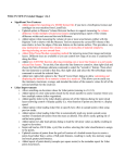
Figure: Z-Order curve based dimensional decomposition
Fortunately there is already a type of transform that describes this operation in mathematics – it’s
called a “Space Filling Curve” – or SFC for short. Different space filling curves have different properties
- what they all do is take a n-dimensional space and describe a set of steps to trace all points in a single
sequence.
Figure: Haverkort, Walderveen Locality and Bounding-Box Quality of Two-Dimensional Space-Filling
Curves 2008 arXiv:0806.4787v2
The trade-offs for the various curves are outside the scope of this user manual, but the paper cited for
figure two is an excellent starting point to start learning about these curves.
For the purposes of GeoWave we have implemented two space fillings curves:
Z-Order SFC
This is also commonly called a GeoHash, or Morton order (and sometimes incorrectly called a Peano
curve). This is the most popular SFC used for multi-dimensional → 1-dimensional mappings – primarily
because it is both intuitive and very easy to implement in code. There are two common ways to
implement this – ideally a bit-interleaving is used (that is what gives rise to the diagram in figure 2) –
imagine we had two numbers, A and B. Let the binary representation of those numbers be A1A2A3 and
B1B2B3. The “bit interleaved” version would be A1B1A2B2A3B3. Since we are working with binary
numbers this gives a “unit cell” of 2x2. If we added dimensions just image the same interleaving, but
another term - C1C2C3, etc. + This is sometimes implemented in base 10 instead of base 2. This
implementation reduces somewhat the locality (“packing property” – or the measure of how close
numbers in n-dimensional space are to numbers in 1-dimensional space). As you might expect a two
dimensional version of this gives a unit cell of 10x10 (for two dimensions) – hence the worse packing.
Hilbert SFC
The Hilbert curve is a bit more complex to work with than the Z-curve – both when calculating and
when performing a decomposition – hence it is less commonly used. Nevertheless it is popular in other
areas in computer science where multiple variables need to be set in a linear order – process
scheduling for one. A simplistic view of a standard projections of the earth mapped to a Hilbert curve
would look something like this – with 4 bits of cardinality per dimension (how many buckets we have)
Figure: Hilbert space filling curve superimposed over a projection of the earth
Note that there are the cardinality (number of buckets per dimensions) has an impact on the resolution
of our Hilbert index. Here we map from -180 to +180 over 16 buckets – so we have resolution of no
better than 360/16, or 22.5 degrees for longitude (and incidentally 11.25 degrees for latitude). This
doesn’t mean we can’t represent values more precisely than this – it just means our initial (coarse)
index – based on SFC ranges – can’t provide resolution any better than this. Adding more bits per
dimensions will increase the precision of the SFC based index.
Decomposition
Core to the concept of SFC based indexing is range decomposition. This is when we take a range
described in multiple dimensions and turn it into a series of 1d ranges.
Figure: Hilbert Ranges
In the figure above we show that we mean by this. The bounding box described by the blue selection
window – or (2,9) → (5,13) will “fully” decompose to 3 ranges – 70-75, 92→99, and 116→121.
It should be noted that sometimes more simplistic algorithms will not fully decompose – but would
instead represent this as 70-121, or even 64→127 (the smallest “unit cell” this box fits in). As you can
see this would result in scanning many extraneous cells.
At some point – with high precision high dimensionality curves – the number of possible unit cells can
become to large too deal with – in this case GeoWaves optimizes this by treating the curve as a “lower
cardinality” curve than it actually is – so the unit cell size might not be 1, but instead 64, 128, 1024, etc.
This allows the user to still achieve high precision when selection windows are small, but not spend an
inordinate amount of time fully decomposing for large selection windows.
Consider a region query asking for all data from:
(1,1) -> (5,4)
This query range is shown at left by a blue bounding box.
What did we do here?
• We broke down the initial region into 4 subregions – Red boxes.
• We broke down each subregion (red box) into 4 sub-sub regions (purple boxes)
• We then broke down each of those purple boxes into green boxes.
• Once we had a decomposed quad which is full contained by the bounding box we
NOTE
stopped decomposing.
• We didn’t bother decomposing regions which didn’t overlap the original search
criteria.
Here we see the query range fully decomposed into the underlying "quads". Note that in some
instances we were able to stop decomposing when the query window fully contained the quad
(segment 3 and segment 8)
Now we have fully transitioned to the 1d number line from the previous set of quads. We have also
rolled together regions which are contiguous.
Screenshots
The screenshots below are of data loaded from the various attributed data sets into a Geowave
instance, processed (in some cases) by a Geowave analytic process, and rendered by Geoserver.
GeoLife
Microsoft research has made available a trajectory data set that contains the GPS coordinates of 182
users over a three year period (April 2007 to August 2012). There are 17,621 trajectories in this data set.
More information on this data set is available at Microsoft Research GeoLife page
GeoLife at city scale
Below are renderings of GeoLife data. They display both the raw points, as well as the results of a
GeoWave kernel density analytic. The data corresponds to Mapbox zoom level 13.
GeoLife at house scale
This data set corresponds to a Mapbox zoom level of 15
Graphic background ©MapBox and ©OpenStreetMap
Graphic background ©MapBox and ©OpenStreetMap
OpenStreetMap GPX Tracks
The OpenStreetMap Foundation has released a large set of user contributed GPS tracks. These are
about 8 years of historical tracks. The data set consists of just under 3 billion (not trillion as some
websites claim) point, or just under one million trajectories.
More information on this data set is available at GPX Planet page
OSM GPX at continent scale
The data below corresponds to a Mapbox zoom level of 6
OSM GPX at world scale
This data set corresponds to a Mapbox zoom level of 3
T-Drive
Microsoft research has made available a trajectory data set that contains the GPS coordinates of 10,357
taxis in Beijing, China and surrounding areas over a one week period. There are approximately 15
million points in this data set.
More information on this data set is available at: Microsoft Research T-drive page
T-drive at city scale
Below are renderings of the t-drive data. They display both the raw points, as well as the results of a
Geowave kernel density analytic. The data corresponds to Mapbox zoom level 12.
T-drive at block scale
This data set corresponds to a Mapbox zoom level of 15
Graphic background©MapBox and ©OpenStreetMap
Graphic background©MapBox and ©OpenStreetMap
T-drive at house scale
This data set corresponds to a Mapbox zoom level of 17
Graphic background©MapBox and ©OpenStreetMap
Graphic background©MapBox and ©OpenStreetMap
Architecture
Overview
At the core of the GeoWave architecture concept is getting data in, and pulling data out – or Ingest and
Query. There are also two types of data persisted in the system – feature data, and metadata. Feature
data is the actual set of attributes and geometries that are stored for later retrieval. Metadata describes
how the data is persisted in the database. The intent is to store the information needed for data
discovery and retrieval in the database – so an existing data store isn’t tied to a bit of configuration on
a particular external server or client – but instead is “self-describing.”
Indexes
The core engine to quickly retrieve data from GeoWave is a SFC (space filling curve) based index. This
index can be configured with several different parameters:
• number of levels
• number of dimensions
• cardinality of each dimension
• dimension type (bounded / unbounded)
• value range of each dimension
More on each of these properties will be described later; this list here is just to give the reader a notion
of what type of configuration information is persisted.
In order to insert data in a datastore the configuration of the index has to be known. The index is
persisted in a special table and is referenced back via table name to a table with data in it. Therefore
queries can retrieve data without requiring index configuration. There is a restriction that only one
index configuration per table is supported - i.e. you can’t store data on both a 2D and 3D index in the
same table. (You could store 2D geometry types in a 3D index though).
Adapters
To store geometry, attributes, and other information a format is needed that describes how to serialize
and deserialize. An interface is provided that handles the serialization and deserialization of features.
A default implementation supporting the GeoTools simple feature type is also included by default.
More on this specific implementation as well as the interface will be detailed later. In the Adapter
persistence table a pointer to the java class (expected to be on the classpath) is stored. This is loaded
dynamically when the data is queried and results are translated to the native data type
Feature Serialization
GeoWave allows the user to create their own data adapters - these not only determine how the data is
actually stored (serialization/deserialization), but also contain a hierarchy of attribute types. The
reason for this hierarchy has to do with extensibility vs. optimization. A data adapter could
theoretically take a dependency on ffmpeg, store the feature as metadata in a video stream, and persist
that value to the database. All questions of sanity of this solution aside, there are some additional
specific issues with the way fine grain filtering is done - specifically due to the iterators. Iterators are
part of the Accumulo extensibility module and allow for arbitrary code to be plugged in directly at the
tablet server level into the core accumulo kernel. With more code in the iterators there is both a
greater chance of crashing (and taking down a tablet server - and possibly an accumulo instance),
greater use of memory (memory used by the iterator / class loader isn’t available for caching, etc., and
a greater O&M debt - the iterators have to be distributed to each client out of band - and require
impersonating the accumulo user (possibly root).
Based on this our target was to minimize the code, and standardize on as few iterators as possible. This
conflicted with the desire to allow maximum flexibility with arbitrary DataAdapters. A middle ground
was found, and this hierarchy was created. Some standardization was put in place around how certain
data types would be stored and serialized, but a "native data" portion was still left in place for
arbitrary data - with the caveat that native data cannot be used in distributed (iterator based) filtering only in client side filtering.
Primary Index Data
These are sets of data which are also used to construct the primary index (space filling curve). They
will typically be geometry coordinates and optionally time - but could be any set of numeric values
(think decomposed feature vectors, etc.). They cannot be null.
Common Index Data
These are a collection of attributes. There can be any number of attributes, but they must conform to
the DimensionField interface - the attribute type must have a FieldReader and a FieldWriter that is
within the classpath of the tablet servers. We provide a basic implementation for these attribute types:
• Boolean
• Byte
• Short
• Float
• Double
• BigDecimal
• Integer
• Long
• BigInteger
• String
• Geometry
• Date
• Calendar
The values that are not part of the primary index can be used for distributed secondary filtering, and
can be null. The values that are associated with the primary index will be used for fine-grained
filtering within an iterator.
Native Data
These can be literally anything. From the point of view of the data adapter they are just a binary (or
Base64) encoded chunk of data. No distributed filtering can be performed on this data except for
Accumulo’s visibility filter - but the client side filtering extensibility point can still be used if necessary.
The Data Adapter has to provide methods to serialize and deserialize these items in the form of Field
Readers and Writers, but it is not necessary to have these methods on the classpath of any Accumulo
nodes.
Statistics
Adapters provide a set of statistics stored within a statistic store. The set of available statistics is
specific to each adapter and the set of attributes for those data items managed by the adapter. Statistics
include:
• Ranges over an attribute, including time.
• Enveloping bounding box over all geometries.
• Cardinality of the number of stored items.
Optional statistics include:
• Histograms over the range of values for an attribute.
• Cardinality of discrete values of an attribute.
Accumulo Key Structure
The above diagram describes the default structure of entries in the Accumulo data store. The index ID
comes directly from the tiered space filling curve implementation. We do not impose a requirement
that data IDs are globally unique but they should be unique for the adapter. Therefore, the pairing of
Adapter ID and Data ID define a unique identifier for a data element. The lengths are stored within the
row ID as 4 byte integers - this enables fully reading the row ID because these IDs can be of variable
length. The number of duplicates is stored within the row ID as well to inform the de-duplication filter
whether this element needs to be temporarily stored to ensure no duplicates are sent to the caller. The
adapter ID is within the Row ID to enforce unique row IDs as a whole row iterator is used to aggregate
fields for the distributable filters. The adapter ID is also used as the column family as the mechanism
for adapter-specific queries to fetch only the appropriate column families.
Statistics
Adapters provide a set of statistics stored within a statistic store. The set of available statistics is
specific to each adapter and the set of attributes for those data items managed by the adapter. Statistics
include:
• Ranges over an attribute, including time.
• Enveloping bounding box over all geometries.
• Cardinality of the number of stored items.
• Histograms over the range of values for an attribute.
• Cardinality of discrete values of an attribute.
Statistics are updated during data ingest and deletion. Range and bounding box statistics reflect the
largest range over time. Those statistics are not updated during deletion. Cardinality-based statistics
are updated upon deletion.
Statistics retain the same visibility constraints as the associated attributes. Thus, there is a set of
statistics for each unique constraint. The statistics store answers each statistics inquiry for a given
adapter with only those statistics matching the authorizations of the requester. The statistics store
merges authorized statistics covering the same attribute.
Table Structure in Accumulo
Re-Computation
Re-computation of statistics is required in three circumstances:
1. As indexed items are removed from the adapter store, the range and envelope statistics may lose
their accuracy if the removed item contains an attribute that represents the minimum or
maximum value for the population.
2. New statistics added to the statistics store after data items are ingested. These new statistics do not
reflect the entire population.
3. Software changes invalidate prior stored images of statistics.
Ingest
Overview
In addition to the raw data to ingest, the ingest process requires an adapter to translate the native data
into a format that can be persisted into the data store. Also, the ingest process requires an Index which
is a definition of all the configured parameters that defines how data translates to row IDs (how it is
indexed) and what common fields need to be maintained within the table to be used by fine-grained
and secondary filters.
The logic within the ingest process immediately ensures that the index and data adapter are persisted
within the Index Store and the Adapter Store to support self-described data discovery, although in
memory implementations of both of these stores are provided for cases when connections to Accumulo
are undesirable in the ingest process (such as if ingesting bulk data in a Map-Reduce job). Then the
flow determines the set of row IDs that the data will need to be inserted in - duplication is essential
under certain circumstances and therefore data may be inserted in multiple locations (for example,
polygons that cross the dateline, or date ranges that cross binning boundaries such as December 31January 1 when binning by year). De-duplication is always performed as a client filter when querying
the data. This will be combined with the actual data in a persistable format (after a translation has
been performed by the adapter) to create a set of mutations.
There is a Writer interface that the data store’s AccumuloOperations will instantiate which specifies
how the mutations will actually be written. The default implementation will wrap an Accumulo
BatchWriter with this interface, but in some cases it could make sense to provide a custom
implementation of the writer - if performing a bulk ingest within the mapper or reducer of a job, it
would be appropriate to define a writer to add the mutations to the context of the bulk ingest rather
than writing live to Accumulo.
Tools Framework
A plugin framework (using SPI based injection) is provided with several input formats and utilities
supported out of the box.
First we’ll show how to build and use the built in formats, and after that describe how to create a new
plugin.
Building
First build the main project after specifynig the dependency versions you’d like to build against.
export BUILD_ARGS="-Daccumulo.version=1.6.0-cdh5.1.4 -Dhadoop.version=2.6.0-cdh5.4.0
-Dgeotools.version=13.0 -Dgeoserver.version=2.7.0 -Dvendor.version=cdh5 -P cloudera" ①
git clone https://github.com/ngageoint/geowave.git ②
cd geowave
mvn install $BUILD_ARGS ③
① Examples of current build args can be seen in the top level .travis.yml file in the env/matrix section
② If you don’t need the complete history and want to speed up the clone you can limit the depth of
your checkout with --depth NUM_COMMITS
③ You can speed up the build by skipping tests by adding -Dfindbugs.skip=true -DskipFormat=true
-DskipITs=true -DskipTests=true
Now we can build the cli tools framework
mvn package -P geowave-tools-singlejar $BUILD_ARGS
The geowave tools jar is now packaged in deploy/target. When packaged for installation there will be a
wrapper script named geowave that will be installed in $PATH. In a development environment where
this script has not been installed you could create a directory containing the tools jar and any needed
plugin jars and use with something like the following command java -cp "$DIR/* <operation>
<options>
geowave -clear
NAME
geowave-clear - Delete existing GeoWave content from Accumulo
SYNOPSIS
geowave -clear <options>
DESCRIPTION
The geowave -clear(1) operator will delete ALL data from a GeoWave namespace, this actually deletes
Accumulo tables prefixed by the given namespace
OPTIONS
-c, --clear
Clear ALL data stored with the same prefix as this namespace (optional; default is to append data to
the namespace if it exists)
-dim, --dimensionality <arg>
The dimensionality type for the index, either 'spatial' or 'spatial-temporal' (optional; default is
'spatial')
-f,--formats <arg>
Explicitly set the ingest formats by name (or multiple comma-delimited formats), if not set all
available ingest formats will be used
-h, --help
Display help
-i, --instance-id <arg>
The Accumulo instance ID
-l, --list
List the available ingest types
-n, --namespace <arg>
The table namespace (optional; default is no namespace)
-p, --password <arg>
The password for the user
-u, --user <arg>
A valid Accumulo user ID
-v, --visibility <arg>
The visibility of the data ingested (optional; default is 'public')
-z, --zookeepers <arg>
A comma-separated list of zookeeper servers that an Accumulo instance is using
geowave -hdfsingest
NAME
geowave-hdfsingest - Load content from an HDFS file system
SYNOPSIS
geowave -hdfsingest <options>
DESCRIPTION
The geowave -hdfsingest(1) operator first copies the local files to an Avro record in HDFS, then
executes the ingest process as a map-reduce job. Data is ingested into Geowave using the
GeowaveInputFormat. This is likely to be the fastest ingest method overall for data sets of any notable
size (or if they have a large ingest/transform cost).
OPTIONS
-b, --base <arg>
Base input file or directory to crawl with one of the supported ingest types
-c, --clear
Clear ALL data stored with the same prefix as this namespace (optional; default is to append data to
the namespace if it exists)
-dim, --dimensionality <arg>
The dimensionality type for the index, either 'spatial' or 'spatial-temporal' (optional; default is
'spatial')
-f,--formats <arg>
Explicitly set the ingest formats by name (or multiple comma-delimited formats), if not set all
available ingest formats will be used
-h, --help
Display help
-hdfs <arg>
HDFS hostname and port in the format hostname:port
-hdfsbase <arg>
The fully qualified path to the base directory in HDFS
-i, --instance-id <arg>
The Accumulo instance ID
-jobtracker <arg>
Hadoop job tracker hostname and port in the format hostname:port
-l, --list
List the available ingest types
-n, --namespace <arg>
The table namespace (optional; default is no namespace)
-p, --password <arg>
The password for the user
-resourceman <arg>
YARN resource manager hostname and port in the format hostname:port
-u, --user <arg>
A valid Accumulo user ID
-v, --visibility <arg>
The visibility of the data ingested (optional; default is 'public')
-x, --extension <arg>
Individual or comma-delimited set of file extensions to accept (optional)
-z, --zookeepers <arg>
A comma-separated list of zookeeper servers that an Accumulo instance is using
ADDITIONAL
The options here are, for the most part, same as for geowave -localingest, with a few additions.
The
hdfs
argument
should
be
the
hostname
and
port,
so
something
like
"hdfs-
namenode.cluster1.com:8020".
The hdfsbase argument is the root path in hdfs that will serve as the base for the stage location. If the
directory doesn’t exist it will be created. The actual ingest file will be created in a "type" (plugin type seen with the --list option) subdirectory under this base directory.
The jobtracker argument is the hostname and port for the jobtracker, so something like mapreducenamenode.cluster1.com:8021
The hdfsstage and poststage options will just be subsets of this comment; the first creating an avro file
in hdfs, the second reading this avro file and ingesting into GeoWave
geowave -hdfsstage
NAME
geowave-hdfsstage - Load supported content from a local file system into HDFS
SYNOPSIS
geowave -hdfsstage <options>
DESCRIPTION
The geowave -hdfsstage(1) operator copies the local files to an Avro record in HDFS
OPTIONS
-b,--base <arg>
Base input file or directory to crawl with one of the supported ingest types
-f,--formats <arg>
Explicitly set the ingest formats by name (or multiple comma-delimited formats), if not set all
available ingest formats will be used
-h,--help
Display help
-hdfs <arg>
HDFS hostname and port in the format hostname:port
-hdfsbase <arg>
Fully qualified path to the base directory in hdfs
-l, --list
List the available ingest types
-x, --extension <arg>
Individual or comma-delimited set of file extensions to accept (optional)
geowave -kafkastage
NAME
geowave-kafkastage - Stage supported files in local file system to a Kafka topic
SYNOPSIS
geowave -kafkastage <options>
DESCRIPTION
The geowave -kafkastage(1) operator will stage supported files in local file system to a Kafka topic
OPTIONS
-b, --base <arg>
Base input file or directory to crawl with one of the supported ingest types
-f,--formats <arg>
Explicitly set the ingest formats by name (or multiple comma-delimited formats), if not set all
available ingest formats will be used
-h, --help
Display help
-kafkaprops <arg>
Properties file containing Kafka properties
-kafkatopic <arg>
Kafka topic name where data will be emitted to
-l, --list
List the available ingest types
-x, --extension <arg>
Individual or comma-delimited set of file extensions to accept (optional)
geowave -localingest
NAME
geowave-localingest - Load content from local file system
SYNOPSIS
geowave -localingest <options>
DESCRIPTION
The geowave -localingest(1) operator will run the ingest code (parse to features, load features to
accumulo) against local file system content.
OPTIONS
-b, --base <arg>
Base input file or directory to crawl with one of the supported ingest types
-c, --clear
Clear ALL data stored with the same prefix as this namespace (optional; default is to append data to
the namespace if it exists)
-dim, --dimensionality <arg>
The dimensionality type for the index, either 'spatial' or 'spatial-temporal' (optional; default is
'spatial')
-f,--formats <arg>
Explicitly set the ingest formats by name (or multiple comma-delimited formats), if not set all
available ingest formats will be used
-h, --help
Display help
-i, --instance-id <arg>
The Accumulo instance ID
-l, --list
List the available ingest types
-n, --namespace <arg>
The table namespace (optional; default is no namespace)
-p, --password <arg>
The password for the user
-u, --user <arg>
A valid Accumulo user ID
-v, --visibility <arg>
The visibility of the data ingested (optional; default is 'public')
-x, --extension <arg>
Individual or comma-delimited set of file extensions to accept (optional)
-z, --zookeepers <arg>
A comma-separated list of zookeeper servers that an Accumulo instance is using
ADDITIONAL
The index type uses one of the two predefined index implementations. You can perform temporal
lookup/filtering with either, but the spatial-temporal includes indexing in the primary index - so will
be more performant if spatial extents are commonly used when querying data.
Visibility is passed to Accumulo as a string, so you should put whatever you want in here.
The namespace option is the GeoWave namespace; this will be the prefix of the GeoWave tables in
Accumulo. There are a few rules for this that derive from geotools/geoserver as well as Accumulo. To
keep it simple if you only use alphabet characters and "_" (underscore) you will be fine.
The extensions argument allows you to override the plugin types, narrowing the scope of what is
passed to the plugins
Finally, the base directory is the root directory that will be scanned on the local system for files to
ingest. The process will scan all subdirectories under the provided directory.
EXAMPLES
List all of the currently registered as ingest type plugins:
geowave -localingest --list
geotools-vector:
tdrive:
files from Microsoft Research T-Drive trajectory data set
geolife:
gpx:
all file-based vector datastores supported within geotools
files from Microsoft Research GeoLife trajectory data set
xml files adhering to the schema of gps exchange format
geotools-raster:
all file-based raster formats supported within geotools
Load some load data
geowave -localingest \
geotools-vector \
-b ./ingest \
-u USERNAME
-i instance \
-p PASSWORD \
-n geowave.50m_admin_0_countries \
-f
-z ZOOKEEPER_HOST_NAME:2181
geowave -poststage
NAME
geowave-poststage - Ingest supported content that has already been staged in HDFS
SYNOPSIS
geowave -poststage <options>
DESCRIPTION
The geowave -poststage(1) operator executes the ingest process as a map-reduce job using data that has
already been staged in an HDFS file system
OPTIONS
-c, --clear
Clear ALL data stored with the same prefix as this namespace (optional; default is to append data to
the namespace if it exists)
-dim, --dimensionality <arg>
The dimensionality type for the index, either 'spatial' or 'spatial-temporal' (optional; default is
'spatial')
-f,--formats <arg>
Explicitly set the ingest formats by name (or multiple comma-delimited formats), if not set all
available ingest formats will be used
-h, --help
Display help
-hdfs <arg>
HDFS hostname and port in the format hostname:port
-hdfsbase <arg>
Fully qualified path to the base directory in HDFS
-i, --instance-id <arg>
The Accumulo instance ID
-jobtracker <arg>
Hadoop job tracker hostname and port in the format hostname:port
-l, --list
List the available ingest types
-n, --namespace <arg>
The table namespace (optional; default is no namespace)
-p, --password <arg>
The password for the user
-resourceman <arg>
YARN resource manager hostname and port in the format hostname:port
-u, --user <arg>
A valid Accumulo user ID
-v, --visibility <arg>
The visibility of the data ingested (optional; default is 'public')
-z,--zookeepers <arg>
A comma-separated list of zookeeper servers that an Accumulo instance is using
geowave -stats
NAME
geowave-stats - Calculate the statistics of an existing GeoWave dataset
SYNOPSIS
geowave -stats <options>
DESCRIPTION
The geowave -stats(1) operator will remove all statistics for an adapter, scan the entire data set and
reconstruct statistics.
OPTIONS
-i, --instance-id <arg>
The Accumulo instance ID
-n, --namespace <arg>
The table namespace (optional; default is no namespace)
-p, --password <arg>
The password for the user
-u, --user <arg>
A valid Accumulo user ID
-v, --visibility <arg>
The visibility of the data ingested (optional; default is 'public')
-z, --zookeepers <arg>
A comma-separated list of zookeeper servers that an Accumulo instance is using
-type <arg>
The name of the feature type to run stats on
-auth <arg>
The authorizations used for the statistics calculation as a subset of the accumulo user authorization;
by default all authorizations are used
EXAMPLES
Given the data we loaded in the geowave -localingest example we could look at the GeoServer Layers
list to obtain the feature type name and recalculate statistics using a command such as the one shown
below.
geowave -stats \
-i accumulo \
ne_50m_admin_0_countries \
-u USERNAME \
-n geowave.50m_admin_0_countries \
-p PASSWORD \
-type
-z ZOOKEEPER_HOST_NAME:2181
geowave -statsdump
NAME
geowave-statsdump - Dump the statistics of an existing GeoWave dataset to standard output
SYNOPSIS
geowave -statsdump <options>
DESCRIPTION
The geowave -statsdump(1) operator will remove all statistics for an adapter, scan the entire data set
and reconstruct statistics.
OPTIONS
-i, --instance-id <arg>
The Accumulo instance ID
-n, --namespace <arg>
The table namespace (optional; default is no namespace)
-p, --password <arg>
The password for the user
-u, --user <arg>
A valid Accumulo user ID
-v, --visibility <arg>
The visibility of the data ingested (optional; default is 'public')
-z, --zookeepers <arg>
A comma-separated list of zookeeper servers that an Accumulo instance is using
-type <arg>
The name of the feature type to run stats on (optional; default is all types)
EXAMPLES
Given the data we loaded in the geowave -localingest example we could look at the GeoServer Layers
list to obtain the feature type name and dump statistics using a command such as the one shown
below.
geowave -statsdump \
ne_50m_admin_0_countries \
-i accumulo \
-u USERNAME \
-n geowave.50m_admin_0_countries \
-p PASSWORD \
-type
-z ZOOKEEPER_HOST_NAME:2181
Ingest Example
We can ingest any data type that has been listed as an ingest plugin. Let’s start out with the GeoTools
datastore; this wraps a bunch of GeoTools supported formats. We will use the shapefile capability for
our example here.
Something recognizable
The naturalearthdata side has a few shapefile we can use use. On the page 50m Cultural Vectors
Let’s download the Admin 0 - Countries shapefile: ne_50m_admin_0_countries.zip
$ mkdir ingest
$ mv ne_50m_admin_0_countries.zip ingest/
$ cd ingest
$ unzip ne_50m_admin_0_countries.zip
$ rm ne_50m_admin_0_countries.zip
$ cd ..
$ geowave -localingest \
-b ./ingest \
-i ACCUMULO_INSTANCE_NAME \
-n geowave.50m_admin_0_countries \ ①
-f geotools-vector \ ②
-u USERNAME \
-p PASSWORD \
-z ZOOKEEPER_HOST_NAME:2181
① We preface the table name with the Accumulo namespace we configured earlier in the Accumulo
configuration section followed by a dot (NAMESPACE.TABLE_NAME)
② Explicitly set the ingest formats by name (or multiple comma-delimited formats), if not set all
available ingest formats will be used
After running the ingest command you should see the various index tables in Accumulo
Ingest plugins
The geowave command line utility comes with several plugins out of the box
geowave -localingest --list
Available ingest types currently registered as plugins:
tdrive:
files from Microsoft Research T-Drive trajectory data set
geotools:
all file-based datastores supported within geotools
geolife:
files from Microsoft Research GeoLife trajectory data set
gpx:
xml files adhering to the schema of gps exchange format
Ingest Statistics and Time Dimension Configuration
The available plugins for vector support adjustments to their configuration via the command line. The
system property 'SIMPLE_FEATURE_CONFIG_FILE' may be assigned to the name of a locally accessible
JSON file defining the configuration.
Example
geowave -DSIMPLE_FEATURE_CONFIG_FILE=myconfigfile.json -localingest
Configuration consists of two parts:
1. Selecting temporal attributes for a temporal index.
2. Assigning to each attribute the type of statistics to be captured within the Statistics Store
The JSON file is made up of configurations. Each configuration is defined by a class name and a set of
attributes
Temporal Configuration
There are three attributes for the temporal configuration:
1. timeName
2. startRangeName
3. endRangeName
These attributes are associated with the name of a simple feature type attribute that references a time
value. To index by a single time attribute, set timeName to the name of the single attribute. To index by
a range, set both startRangeName and endRangeName to the names of the simple feature type attributes
that define start and end time values.
Statistics Configuration
Each simple feature type attribute may have several assigned statistics. Bounding box and range
statistics are automatically captured for Geometry and temporal attributes.
Attribute Type
Statistic Name
Statistic Configuration Statistic Class
Attributes (with
default values)
Numeric
Fixed Bin Histogram
minValue=∞,maxValue=∞,bins=32
String
Example
mil.nga.giat.geowave.ad
apter.vector.stats.Featur
eFixedBinNumericStatis
tics$FeatureFixedBinCo
nfig
Dynamic Histogram
mil.nga.giat.geowave.ad
apter.vector.stats.Featur
eNumericHistogramStat
istics$FeatureNumericH
istogramConfig
Numeric Range
mil.nga.giat.geowave.ad
apter.vector.stats.Featur
eNumericRangeStatistic
s$FeatureNumericRange
Config
Count Min Sketch
errorFactor=0.001,proba mil.nga.giat.geowave.ad
bilityOfCorrectness=0.98 apter.vector.stats.Featur
eCountMinSketchStatisti
cs$FeatureCountMinSke
tchConfig
Hyper Log Log
precision=16
mil.nga.giat.geowave.ad
apter.vector.stats.Featur
eHyperLogLogStatistics$
FeatureHyperLogLogCo
nfig
{
"configurations": [
{"@class":"mil.nga.giat.geowave.adapter.vector.utils.TimeDescriptors$TimeDescriptorC
onfiguration",
"startRangeName":null,
"endRangeName":null,
"timeName":"captureTime"
},
{"@class":"mil.nga.giat.geowave.adapter.vector.stats.StatsConfigurationCollection$Si
mpleFeatureStatsConfigurationCollection",
"attConfig" : {
"population" : {
"configurationsForAttribute" : [
{"@class" :
"mil.nga.giat.geowave.adapter.vector.stats.FeatureFixedBinNumericStatistics$FeatureFixedB
inConfig","bins" : 24}
]
},
"country" : {
"configurationsForAttribute" : [
{"@class" :
"mil.nga.giat.geowave.adapter.vector.stats.FeatureCountMinSketchStatistics$FeatureCountMi
nSketchConfig",
"probabilityOfCorrectness" : 0.98,
"errorFactor" :0.001
},
{"@class" :
"mil.nga.giat.geowave.adapter.vector.stats.FeatureHyperLogLogStatistics$FeatureHyperLogLo
gConfig"}
]
}
}
}
]
}
New Formats
There are multiple ways to get data into GeoWave. In other sections we will discuss higher order
frameworks, mapreduce interfaces, etc. The intent here is "just the basics" - what’s the least framework
intensive way that one can load geospatial data.
Information here will reference the SimpleIngest and SimpleIngestProducerConsumer examples in the
geowave-examples project.
Minimum information needed
Geowave requires a few pieces of fundamental information in order to persist data - these are:
• BasicAccumuloOperations object
• This class contains the information required to connect to an accumulo instance - and which table
to use in accumulo.
◦ Zookeepers - in the format zookeeper1:port,zookeeper2:port,etc…
◦ Accumulo Instance ID - this is the "instance" that the Accumulo cluster you are connecting to
was initialized with. It’s a global setting per cluster.
◦ Accumulo Username - this is the name of the user you would like to connect as. This is a user
account managed by accumulo, not a system, etc. user.
◦ Accumulo Password - this is the password associated with the user specified above. Again, this
is an accumulo controlled secret.
◦ Geowave Namespace - this is not an Accumulo namespace; rather think of it as a prefix
geowave will use on any tables it creates. The only current constraint is only one index type is
allowed per namespace.
• SimpleFeatureType instance
• Simple Feature Types are an OGC specification for defining geospatial features. Leveraging this
standard is one of the easiest ways to get GIS data into GeoWave
• SimpleFeatureType instance - org.opengis.feature.simple.SimpleFeatureType - this defines the
names, types, and other metadata (nullable, etc) of a feature. Think of it as a Map of Name:Values
where the values are typed.
• DataAdapter instance
• A geowave data adapter is an implementation of the DataAdapter interface that handles the
persistence serialization of whatever the object you are storing.
• We are storing SimpleFeatures, so can leverage the provided FeatureDataAdapter
• Index instance
• The final piece needed - the index defines which attributes are indexed, and how that index is
constructed.
• There are lots of options for index configuration, but for convenience we have provided two
defaults
• DataStore
• This is the piece that puts everything above together.
• Initialization required a BasicAccumuloOperations instance, the rest are provided as parameters
for calls which need them.
Ingest some data
Here we will programmatically generate a grid of points at each location where a whole number
latitude and longitude intersect.
Basic Accumulo Operations
/***
* The class tells geowave about the accumulo instance it should connect to, as well as
what tables it should create/store it's data in
* @param zookeepers Zookeepers associated with the accumulo instance, comma separate
* @param accumuloInstance Accumulo instance name
* @param accumuloUser
User geowave should connect to accumulo as
* @param accumuloPass
Password for user to connect to accumulo
* @param geowaveNamespace
Different than an accumulo namespace (unfortunate naming
usage) - this is basically a prefix on the table names geowave uses.
* @return Object encapsulating the accumulo connection information
* @throws AccumuloException
* @throws AccumuloSecurityException
*/
protected BasicAccumuloOperations getAccumuloInstance(String zookeepers, String
accumuloInstance, String accumuloUser, String accumuloPass, String geowaveNamespace)
throws AccumuloException, AccumuloSecurityException {
return new BasicAccumuloOperations(zookeepers, accumuloInstance, accumuloUser,
accumuloPass, geowaveNamespace);
}
Simple Feature Type
We know fore sure we need a geometry field. Everything else is really optional. It’s often convenient to
add a text latitude and longitude field for ease of display values (getFeatureInfo, etc.).
/***
* A simple feature is just a mechanism for defining attributes (a feature is just a
collection of attributes + some metadata)
* We need to describe what our data looks like so the serializer (FeatureDataAdapter for
this case) can know how to store it.
* Features/Attributes are also a general convention of GIS systems in general.
* @return Simple Feature definition for our demo point feature
*/
protected SimpleFeatureType createPointFeatureType(){
final SimpleFeatureTypeBuilder builder = new SimpleFeatureTypeBuilder();
final AttributeTypeBuilder ab = new AttributeTypeBuilder();
//Names should be unique (at least for a given GeoWave namespace) - think about names
in the same sense as a full classname
//The value you set here will also persist through discovery - so when people are
looking at a dataset they will see the
//type names associated with the data.
builder.setName("Point");
//The data is persisted in a sparse format, so if data is nullable it will not take
up any space if no values are persisted.
//Data which is included in the primary index (in this example lattitude/longtiude)
can not be null
//Calling out latitude an longitude separately is not strictly needed, as the
geometry contains that information. But it's
//convienent in many use cases to get a text representation without having to handle
geometries.
builder.add(ab.binding(Geometry.class).nillable(false).buildDescriptor("geometry"));
builder.add(ab.binding(Date.class).nillable(true).buildDescriptor("TimeStamp"));
builder.add(ab.binding(Double.class).nillable(false).buildDescriptor("Latitude"));
builder.add(ab.binding(Double.class).nillable(false).buildDescriptor("Longitude"));
builder.add(ab.binding(String.class).nillable(true).buildDescriptor("TrajectoryID"));
builder.add(ab.binding(String.class).nillable(true).buildDescriptor("Comment"));
return builder.buildFeatureType();
}
Spatial index
/***
* We need an index model that tells us how to index the data - the index determines
* -What fields are indexed
* -The precision of the index
* -The range of the index (min/max values)
* -The range type (bounded/unbounded)
* -The number of "levels" (different precisions, needed when the values indexed has
ranges on any dimension)
* @return GeoWave index for a default SPATIAL index
*/
protected Index createSpatialIndex(){
//Reasonable values for spatial and spatio-temporal are provided through static
factory methods.
//They are intended to be a reasonable starting place - though creating a custom
index may provide better
//performance is the distribution/characterization of the data is well known.
return IndexType.SPATIAL.createDefaultIndex();
}
Data Adapter
/***
* The dataadapter interface describes how to serialize a data type.
* Here we are using an implementation that understands how to serialize
* OGC SimpleFeature types.
* @param sft simple feature type you want to generate an adapter from
* @return data adapter that handles serialization of the sft simple feature type
*/
protected FeatureDataAdapter createDataAdapter(SimpleFeatureType sft){
return new FeatureDataAdapter(sft);
}
Generating and loading points
protected void generateGrid(
final BasicAccumuloOperations bao ) {
// create our datastore object
final DataStore geowaveDataStore = getGeowaveDataStore(bao);
// In order to store data we need to determine the type of data store
final SimpleFeatureType point = createPointFeatureType();
// This a factory class that builds simple feature objects based on the
// type passed
final SimpleFeatureBuilder pointBuilder = new SimpleFeatureBuilder(
point);
// This is an adapter, that is needed to describe how to persist the
// data type passed
final FeatureDataAdapter adapter = createDataAdapter(point);
// This describes how to index the data
final Index index = createSpatialIndex();
// features require a featureID - this should be unqiue as it's a
// foreign key on the feature
// (i.e. sending in a new feature with the same feature id will
// overwrite the existing feature)
int featureId = 0;
// get a handle on a GeoWave index writer which wraps the Accumulo
// BatchWriter, make sure to close it (here we use a try with resources
// block to close it automatically)
try (IndexWriter indexWriter = geowaveDataStore.createIndexWriter(index)) {
// build a grid of points across the globe at each whole
// lattitude/longitude intersection
for (int longitude = -180; longitude <= 180; longitude++) {
for (int latitude = -90; latitude <= 90; latitude++) {
pointBuilder.set(
"geometry",
GeometryUtils.GEOMETRY_FACTORY.createPoint(new Coordinate(
longitude,
latitude)));
pointBuilder.set(
"TimeStamp",
new Date());
pointBuilder.set(
"Latitude",
latitude);
pointBuilder.set(
"Longitude",
longitude);
// Note since trajectoryID and comment are marked as
// nillable we
// don't need to set them (they default ot null).
final SimpleFeature sft = pointBuilder.buildFeature(String.valueOf
(featureId));
featureId++;
indexWriter.write(
adapter,
sft);
}
}
}
catch (final IOException e) {
log.warn(
"Unable to close index writer",
e);
}
}
Other methods
There are other patterns that can be used - see the various classes in the geowave-examples project.
The
method
displayed
above
is
the
suggested
pattern
but
are
more
-
it’s
demonstrated
in
SimpleIngestIndexWriter.java
The
other
methods
displayed
work,
either
complicated
(SimpleIngestProducerConsumer.java) or not very efficient (SimpleIngest.java).
than
necessary
Analytics
Overview
Analytics embody algorithms tailored to geospatial data. Most analytics leverage Hadoop MapReduce
for bulk computation. Results of analytic jobs consist of vector or raster data stored in GeoWave. The
analytics infrastructure provides tools to build algorithms in Spark.
For example, a Kryo
serializer/deserializer enables exchange of SimpleFeatures and the GeoWaveInputFormat supplies
data to the Hadoop RDD <1>.
① GeoWaveInputFormat does not remove duplicate features that reference polygons spanning
multiple index regions.
The following algorithms are provided.
Name
Description
KMeans++
A K-Means implementation to find K centroids over the population of data. A set of
preliminary sampling iterations find an optimal value of K and the an initial set of K
centroids. The algorithm produces K centroids and their associated polygons. Each
polygon represents the concave hull containing all features associated with a
centroid. The algorithm supports drilling down multiple levels. At each level, the set
centroids are determined from the set of features associated the same centroid from
the previous level.
KMeans Jump
Uses KMeans++ over a range of k, choosing an optimal k using an information
theoretic based measurement.
DBScan
The Density Based Scanner algorithm produces a set of convex polygons for each
region meeting density criteria. Density of region is measured by a minimum
cardinality of enclosed features within a specified distance from each other.
Nearest
Neighbors
A infrastructure component that produces all the neighbors of a feature within a
specific distance.
Building
First build the main project, specifying the dependency versions.
export BUILD_ARGS="-Daccumulo.version=1.6.0-cdh5.1.4 -Dhadoop.version=2.6.0-cdh5.4.0
-Dgeotools.version=13.0 -Dgeoserver.version=2.7.0 -Dvendor.version=cdh5 -P cloudera"
git clone https://github.com/ngageoint/geowave.git
cd geowave
mvn install -Dfindbugs.skip=true -DskipFormat=true -DskipITs=true -DskipTests=true
$BUILD_ARGS
Next, build the analytics tool framework.
cd analytics/mapreduce
mvn package -P analytics-singlejar -Dfindbugs.skip=true -DskipFormat=true -DskipITs=true
-DskipTests=true $BUILD_ARGS
Running
The 'singlejar' jar file is located in the analytics/mapreduce/target/munged.
The jar is executed by
Yarn.
yarn jar geowave-analytic-mapreduce-0.8.8-SNAPSHOT-analytics-singlejar.jar -dbscan -n
rwgdrummer.gpx -u rwgdrummer -p rwgdrummer -z zookeeper-master:2181 -i accumulo -emn 2
-emx 6 -pd 1000 -pc
mil.nga.giat.geowave.analytic.partitioner.OrthodromicDistancePartitioner -cms 10 -orc 4
-hdfsbase /user/rwgdrummer -b bdb4 -eit gpxpoint
Parameters
This set of parameters is not complete. There are many parameters that permit customizations such as
distance functions, partitioning and sampling.
Argument
Description
-n
Namespace
-u
Accumulo User
-p
Accumulo User Password
-z
Zookeeper host and port
-i
Accumulo instance name
-emn
Minimum input splits
-emx
Maximum input splits (controls the number of Hadoop Mappers).
-eit
The type name of the input features to analyze.
-eot
The type name of the output features (e.g. cluster polygons and points).
-eq
A CQL query string to constrain the extracted data from GeoWave for analysis.
-pd
Maximum distance in meters for features in a cluster.
-pc
Partitioning algorithm for Nearest Neighbors and DBScan algorithms.
-sms
Minimum sample size (e.g. for choosing K)
Argument
Description
-sxs
Maximum sample size (e.g. for choosing K.)
-ssi
Minumum number of sample iterations.
-jrc
Comma separated range of centroids (e.g. 2,10) for KMeans-Jump.
-jkp
The minimum sample size (within the range provide by jrc parameter, where
KMeans++ performs sampling, rather than using a single random sample.
-cms
Minimum density of a cluster.
-cmi
Maximum number of KMeans clustering iterations. KMeans usually converges on a
solution with this constraint. A value of between 3 and 10 is often sufficient.
-crc
Number of reducers to process extracted data in KMeans.
-orc
Number of reducers to load clusters into GeoWave.
-hdfsbase
Location in HBase to store intermediate results.
-b
Batch Identifier. Each algorithm can be run within multiple configurations, each
representing a different batch.
-zl
The number of 'zoom' levels in KMeans Clustering algorithms.
Query
Overview
A query in GeoWave currently consists of a set of ranges on the dimensions of the primary index. Up to
3 dimensions (plus temporal optionally) can take advantage of any complex OGC geometry for the
query window. For dimensions of 4 or greater the query can only be a set of ranges on each dimension
(i.e. hyper-rectangle, etc.).
The query geometry is decomposed by GeoWave into a series of ranges on a one dimensional number
line - based on a compact Hilbert space filling curve ordering. These ranges are sent through an
Accumulo batch scanner to all the tablet servers. These ranges represent the coarse grain filtering.
At the same time the query geometry has been serialized and sent to custom Accumulo iterators. These
iterators then do a second stage filtering on each feature for an exact intersection test. Only if the
stored geometry and the query geometry intersect does the processing chain continue.
A second order filter can then be applied - this is used to remove features based on additional
attributes - typically time or other feature attributes. These operators can only exclude items from the
set defined by the range - they cannot include additional features. Think "AND" operators - not "OR".
A final filter is possible on the client set - after all the returned results have been aggregated together.
Currently this is only used for final deduplication. Whenever possible the distributed filter options
should be used - as it splits the work load among all the tablet servers.
Third Party
GeoServer
Geowave supports both raster images and vector data exposed through Geoserver.
WFS-T
Extending Geotools, Geowave supports WFS-T for vector data. After following the deployment steps,
Geowave appears as a data store type called 'GeoWave Datastore'.
On the Geowave data store creation tab, the system prompts for the following properties.
Name
Description
Constraints
ZookeeperServers
Comma-separated list of
Zookeeper host and port.
Host and port are separated by a
colon (host:port).
InstanceName
The Accumulo tablet server’s
instance name.
The name matches the one
configured in Zookeeper.
UserName
The Accumulo user name.
The user should have
administrative privileges to add
and remove authorized visibility
constraints.
Password
Accumulo user’s password.
Namespace
The table namespace associated
with this Accumlo data store
Lock Management
Select one from a list of lock
managers.
Authorization Management
Provider
Select from a list of providers.
Authorization Data URL
The URL for an external
supporting service or
configuration file.
The interpretation of the URL
depends on the selected
provider.
Transaction Buffer Size
The maximum number of newly
inserted features per transaction
buffered in memory prior to
transaction completion.
Considerations include system
memory, size of typical
transactions, the expected
number of simultaneous
transactions and the average
size of a new feature.
Zookeeper is required with a
multiple Geoserver architecture.
Transactions
Transactions are initiated through a Transaction operation, containing inserts, updates and deletes to
features. WFS-T supports feature locks across multiple requests by using a lock request followed by
subsequent use of a provided lock ID. The Geowave implementation supports transaction isolation.
Consistency during a commit is not fully supported. Thus, a failure during a commit of a transaction
may leave the affected data in an intermediary state—some deletions, updates or insertions may not be
processed. The client application must implement its on compensation logic upon receiving a committime error response. As expected with Accumulo, operations on a single feature instances are atomic.
Inserted features are buffered prior to commit. The features are bulk fed to the data store when the
buffer size is exceeded and when the transaction is committed. In support of atomicity and isolation,
flushed features, prior to commit, are marked in a transient state, only visible to the controlling
transaction. Upon commit, these features are 'unmarked'. The overhead incurred by this operation is
avoided by increasing the buffer size to avoid pre-commit flushes.
Lock Management
Lock management supports life-limited locks on feature instances. There are only two supported lock
managers: in memory and Zookeeper. Memory is suitable for single Geoserver instance installations.
Index Selection
Data written through WFS-T is indexed within a single index. The adapter inspects existing indices,
finding one that matches the data requirements. A geo-temporal index is chosen for features with
temporal attributes. The adapter creates a geo-spatial index upon failure of finding a suitable index.
Geo-temporal index is not created, regardless of the existence of temporal attributes. Currently, geotemporal indices lead to poor performance for queries requesting vectors over large spans of time.
Authorization Management
Authorization Management provides the set of credentials compared against the security labels
attached to each cell. Authorization Management determines the set of authorizations associated with
each WFS-T request. The available Authorization Management strategies are registered through the
Server
Provider
model,
within
the
file
META-
INF/services/mil.nga.giat.geowave.vector.auth.AuthorizationFactorySPI.
The provided implementations include the following: . Empty - Each request is processed without
additional authorization. . JSON - The requester user name, extracted from the Security Context, is used
as a key to find the user’s set of authorizations from a JSON file. The location of the JSON file is
determined by the associated Authorization Data URL (e.g. file://opt/config/auth.json). An example of
the contents of the JSON file is given below.
{
"authorizationSet": {
"fred" : ["1","2","3"],
"barney" : ["a"]
}
}
Fred has three authorization labels. Barney has one.
Visibility Management
Visibility constraints, applied to feature instances during insertions, are ultimately determined a
mil.nga.giat.geowave.store.data.field.FieldWriter, of which there are writers for each supported
data type in Geoserver. By default, the set visibility expression attached to each feature property is
empty. Visibility Management supports selection of a strategy by wrapping each writer to provide
visibility. This alleviates the need to extend the type specific FieldWriters.
The visibility management strategy is registered through the Java Server Provider model, within in the
file META-INF/services/mil.nga.giat.geowave.vector.plugin.visibility.ColumnVisibilityManagement. The
only provided implementation is the JsonDefinitionColumnVisibilityManagement. The implementation
expects an property within each feature instance to contain a JSON string describing how to set the
visibility for each property of the feature instance. This approach allows each instance to determine its
own visibility criteria.
Each name/value pair within the JSON structure defines the visibility for the associated feature
property with the same name. In the following example, the geometry property is given a visibility S;
the eventName is given a visibility TS.
{ "geometry" : "S", "eventName": "TS" }
JSON attributes can be regular expressions, matching more than one feature property name. In the
example, all properties except for those that start with 'geo' have visibility TS.
{ "geo.*" : "S", ".*" : "TS" }
The order of the name/value pairs must be considered if one rule is more general than another, as
shown in the example. The rule . matches all properties. The more specific rule geo. must be
ordered first.
The system extracts the JSON visibility string from a feature instance property named
GEOWAVE_VISIBILITY. Selection of an alternate property is achieved by setting the associated attribute
descriptor 'visibility' to the boolean value TRUE.
Statistics
The adapter captures statistics for each numeric, temporal and geo-spatial attribute. Statistics are used
to constrain queries and answer inquiries by GeoServer for data ranges, as required for map requests
and calibration of zoom levels in Open Layers.
Installation from RPM
Overview
There is a public GeoWave RPM Repo available with the following packages. As you’ll need to
coordinate a restart of Accumulo to pick up changes to the GeoWave iterator classes the repos default
to be disabled so you can keep auto updates enabled. When ready to do an update simply add
--enablerepo=geowave to your command. The packages are built for a number of different hadoop
distributions (Cloudera, Hortonworks and Apache) the RPMs have the vendor name embedded as the
second portion of the rpm name (geowave-apache-accumulo, geowave-hdp2-accumulo or geowavecdh5-accumulo)
Examples
# Use GeoWave repo RPM to configure a host and search for GeoWave RPMs to install
# Several of the rpms (accumulo, jetty and tools) are both GeoWave version and vendor
version specific
# In the examples below the rpm name geowave-$VERSION-VENDOR_VERSION would be adjusted as
needed
rpm -Uvh http://s3.amazonaws.com/geowave-rpms/release/noarch/geowave-repo-1.03.noarch.rpm
yum --enablerepo=geowave search geowave-0.8.7-cdh5
# Install GeoWave Accumulo iterator on a host (probably a namenode)
yum --enablerepo=geowave install geowave-0.8.7-cdh5-accumulo
# Update
yum --enablerepo=geowave install geowave-0.8.7-cdh5-*
Table 1. GeoWave RPMs
Name
Description
geowave-*-accumulo
Accumulo Components
geowave-*-core
Core (home directory and geowave user)
geowave-*-docs
Documentation (HTML, PDF and man pages)
geowave-*-tools
Command Line Tools (ingest, etc.)
geowave-*-jetty
GeoServer components installed into
/usr/local/geowave/geoserver and available at
http://FQDN:8080/geoserver
geowave-*-puppet
Puppet Scripts
Name
Description
geowave-*-single-host
All GeoWave Components installed on a single
host (sometimes useful for development)
geowave-repo
GeoWave RPM Repo config file
geowave-repo-dev
GeoWave Development RPM Repo config file
RPM Installation Notes
RPM names contain the version in the name so support concurrent installations of multiple GeoWave
and/or vendor versions. A versioned /usr/local/geowave-$GEOWAVE_VERSION-$VENDOR_VERSION
directory
is
linked
to
/usr/local/geowave
using
alternatives
ex:
/usr/local/geowave
→
/usr/local/geowave-0.8.7-hdp2 but there could also be another /usr/local/geowave-0.8.6-cdh5 still
installed but not the current default.
View geowave-home installed and default using alternatives
alternatives --display geowave-home
geowave-home - status is auto.
link currently points to /usr/local/geowave-0.8.7-hdp2
/usr/local/geowave-0.8.7-hdp2 - priority 87
/usr/local/geowave-0.8.6-cdh5 - priority 86
Current `best' version is /usr/local/geowave-0.8.7-hdp2.
geowave-*-accumulo: This RPM will install the GeoWave Accumulo iterator into the local file system
and then upload it into HDFS using the hadoop fs -put command. This means of deployment requires
that the RPM is installed on a node that has the correct binaries and configuration in place to push files
to HDFS, like your namenode. We also need to set the ownership and permissions correctly within
HDFS and as such need to execute the script as a user that has superuser permisisons in HDFS. This
user varies by Hadoop distribution vendor. If the Accumulo RPM installation fails, check the install log
located at /usr/local/geowave/accumulo/geowave-to-hdfs.log for errors. The script can be re-run
manually if there was a problem that can be corrected like the HDFS service was not started. If a nondefault user was used to install Hadoop you can specify a user that has permissions to upload with the
--user argument /usr/local/geowave/accumulo/deploy-to-geowave-to-hdfs.sh --user my-hadoop-user
With the exception of the Accumulo RPM mentioned above there are no restrictions on where you
install RPMs. You can install the rest of the RPMs all on a single node for development use or a mix of
nodes depending on your cluster configuration.
Maven Repositories
Overview
There are public maven repositories available for both release and snapshot geowave artifacts (no
transitive dependencies). Automated deployment is available, but requires a S3 access key (typically
added to your ~/.m2/settings.xml)
Maven POM fragments
Releases
<repository>
<id>geowave-maven-releases</id>
<name>GeoWave AWS Release Repository</name>
<url>http://geowave-maven.s3-website-us-east-1.amazonaws.com/release</url>
<releases>
<enabled>true</enabled>
</releases>
<snapshots>
<enabled>false</enabled>
</snapshots>
</repository>
Snapshots
<repository>
<id>geowave-maven-snapshot</id>
<name>GeoWave AWS Snapshot Repository</name>
<url>http://geowave-maven.s3-website-us-east-1.amazonaws.com/snapshot</url>
<releases>
<enabled>false</enabled>
</releases>
<snapshots>
<enabled>true</enabled>
</snapshots>
</repository>
Maven settings.xml fragments
(you probably don’t need this unless you are deploying official GeoWave artifacts)
Snapshots
<servers>
<server>
<id>geowave-maven-releases</id>
<username>ACCESS_KEY_ID</username>
<password>SECRET_ACCESS_KEY</password>
</server>
<server>
<id>geowave-maven-snapshots</id>
<username>ACCESS_KEY_ID</username>
<password>SECRET_ACCESS_KEY</password>
</server>
</servers>
Installation from Source
GeoServer
GeoServer Versions
GeoWave has to be built against specific versions of GeoWave and GeoTools. To see the currently
supported versions look at the build matrix section of the .travis.yml file in the root directory of the
project. All of the examples below use the variable $BUILD_ARGS to represent your choice of all the
dependency versions.
Example build args:
export BUILD_ARGS="-Daccumulo.version=1.6.0 -Dhadoop.version=2.5.0-cdh5.3.0
-Dgeotools.version=13.0 -Dgeoserver.version=2.7.0 -Dvender.version=cdh5 -P cloudera"
GeoServer Install
First we need to build the GeoServer plugin - from the GeoWave root directory:
mvn package -P geotools-container-singlejar $BUILD_ARGS
let’s assume you have GeoServer deployed in a Tomcat container in /opt/tomcat
cp deploy/target/*-geoserver-singlejar.jar /opt/tomcat/webapps/geoserver/WEB-INF/lib/
and re-start Tomcat
Accumulo
Accumulo Versions
GeoWave has been tested and works against accumulo 1.5.0, 1.5.1, 1.6.0 and 1.6.1 Ensure you’ve set the
desired version in the BUILD_ARGS environment variable
Accumulo Install
mvn package -P accumulo-container-singlejar $BUILD_ARGS
Accumulo Configuration
Overview
The two high level tasks to configure Accumulo for use with GeoWave are to ensure the memory
allocations for the master and tablet server processes are adequate and to add the GeoWave Accumulo
iterator to a classloader. The iterator is a rather large file so ensure the Accumulo Master process has at
least 512m of heap space and the Tablet Server processes have at least 1g of heap space.
The recommended Accumulo configuration for GeoWave requires several manual configuration steps
but isolates the GeoWave libraries in application specific classpath(s) reducing the possibility of
dependency conflict issues. A single user for all of geowave data or a user per data type are two of the
many local configuration options just ensure each namespace containing GeoWave tables is configured
to pick up the geowave-accumulo.jar.
Procedure
1. Create a user and namespace
2. Grant the user ownership permissions on all tables created within the application namespace
3. Create an application or data set specific classpath
4. Configure all tables within the namespace to use the application classpath
accumulo shell -u root
createuser geowave ①
createnamespace geowave
grant NameSpace.CREATE_TABLE -ns geowave -u geowave ②
config -s
general.vfs.context.classpath.geowave=hdfs://NAME_NODE_FQDN:8020/ACCUMULO_ROOT/classpath/
geowave/VERSION_AND_VENDOR_VERSION/[^.].*.jar ③
config -ns geowave -s table.classpath.context=geowave ④
exit
① You’ll be prompted for a password
② Ensure the user has ownership of all tables created within the namespace
③ The Accumulo root path in HDFS varies between hadoop vendors. Cloudera is /accumulo and
Hortonworks is /apps/accumulo
④ Link the namespace with the application classpath, adjust the labels as needed if you’ve used
different user or appilcation names
These manual configuration steps have to be performed before attempting to create GeoWave index
tables. After the initial configuration you may elect to do further user and namespace creation and
configuring to provide isolation between groups and data sets.
Managing
After installing a number of different iterators you may want to figure out which iterators have been
configured.
# Print all configuration and grep for line containing vfs.context configuration and also
show the following line
accumulo shell -u root -p ROOT_PWD -e "config -np" | grep -A 1
general.vfs.context.classpath
You will get back a listing of context classpath override configurations which map the application or
user context you configured to a specific iterator jar in HDFS.
Versioning
It’s of critical importance to ensure that the various GeoWave components are all the same version and
that your client is of the same version that was used to write the data.
Basic
The RPM packaged version of GeoWave puts a timestamp in the name so it’s pretty easy to verify that
you have a matched set of RPMs installed. After an update of the components you must restart
Accumulo to get vfs to download the new versions and this should keep everything synched.
Compare version and timestamps of installed RPMs
[spohnae@c1-master ~]$ rpm -qa | grep geowave
geowave-0.8.7-hdp2-core-0.8.7-201505131644.noarch
geowave-0.8.7-hdp2-jetty-0.8.7-201505131644.noarch
geowave-0.8.7-hdp2-accumulo-0.8.7-201505131644.noarch
geowave-0.8.7-hdp2-tools-0.8.7-201505131644.noarch
Advanced
When GeoWave tables are first accessed on a tablet server the vfs classpath tells Accumulo where to
download the jar file from HDFS. The jar file is copied into the local /tmp directory (the default
general.vfs.cache.dir setting anyway) and loaded onto the classpath. If there is ever doubt as to if these
versions match you can use the commands below from a tablet server node to verify the version of this
artifact.
Commit hash of the jar in HDFS
sudo -u hdfs hadoop fs -cat /accumulo/classpath/geowave/geowave-accumulo-build.properties
| grep scm.revision | sed s/project.scm.revision= ①
① The root directory of Accumulo in various distributions can vary, check with hadoop fs -ls / first to
ensure you have the correct initial path
Compare with the versions downloaded locally
sudo find /tmp -name "*geowave-accumulo.jar" -exec unzip -p {} build.properties
grep scm.revision | sed s/project.scm.revision=//
\; |
Example
[spohnae@c1-node-03 ~]$ sudo -u hdfs hadoop fs -cat
/ACCUMULO_ROOT/classpath/geowave/VERSION_AND_VENDOR_VERSION/geowave-accumulobuild.properties | grep scm.revision | sed s/project.scm.revision=//
294ffb267e6691de3b9edc80e312bf5af7b2d23f ①
[spohnae@c1-node-03 ~]$ sudo find /tmp -name "*geowave-accumulo.jar" -exec unzip -p {}
build.properties \; | grep scm.revision | sed s/project.scm.revision=//
294ffb267e6691de3b9edc80e312bf5af7b2d23f ②
294ffb267e6691de3b9edc80e312bf5af7b2d23f ②
25cf0f895bd0318ce4071a4680d6dd85e0b34f6b
① This is the version loaded into hdfs and should be present on all tablet servers once Accumulo has
been restarted
② The find command will probably locate a number of different versions depending on how often
you clean out /tmp.
There may be multiple versions copies present, one per JVM, the error scenario is when a tablet server
is missing the correct iterator jar.
Building
GeoWave will shortly be available in maven central (for tagged releases), but until then - or to get the
latest features - building GeoWave from source is the best bet.
Application Dependencies
This ultra quickstart assumes you have installed and configured:
• Git
• Java JDK (>= 1.7). The OracleJDK is the most thoroughly tested, but there are no known issues with
OpenJDK.
• Maven >= 3.2.1
• GeoServer instance >= 2.5.2 (due to: GEOT-4587)
• Apache Accumulo version 1.5 or greater is required. 1.5.0, 1.5.1, and 1.6.0 have all been tested.
• Apache Hadoop versions 1.x and 2.x should all work. The software has specifically been run on:
• Cloudera CDH4 and CDH5 (MR1)
• Hortonworks Data Platform 2.1.
• MapReduce 1 with the new API (org.apache.hadoop.mapreduce.*) is used. Testing is underway
against YARN / MR2 and seems to be positive, but well, it’s still underway.
• Java Advanced Imaging and Java Image I/O are also both required to be installed on the GeoServer
instance(s) as well as on the Accumulo nodes. The Accumulo support is only required for certain
functions (distributed rendering) - so this may be skipped in some cases.
Maven dependencies
Required repositories not in Maven Central have been added to the parent POM. Specifically the
cloudera and opengeo repos.
Build Process
Checkout geowave, set your preferred dependencies as build arguments and then run maven install.
export BUILD_ARGS="-Daccumulo.version=1.6.0-cdh5.1.4 -Dhadoop.version=2.6.0-cdh5.4.0
-Dgeotools.version=13.0 -Dgeoserver.version=2.7.0 -Dvendor.version=cdh5 -P cloudera" ①
git clone https://github.com/ngageoint/geowave.git ②
cd geowave
mvn install $BUILD_ARGS ③
① Examples of current build args can be seen in the top level .travis.yml file in the env/matrix section
② If you don’t need the complete history and want to speed up the clone you can limit the depth of
your checkout with --depth NUM_COMMITS
③ You can speed up the build by skipping tests by adding -Dfindbugs.skip=true -DskipFormat=true
-DskipITs=true -DskipTests=true
Integration Tests: Windows
NOTE
Integration tests are currently not working on Windows out of the box. If you install
cygwin and set the environmental variable CYGPATH to the location of the cygpath
binary provided by cygwin then is should work. Eclipse and Avro generated files
Docker Build Process
We have preliminary support for building both the GeoWave jar artifacts and RPMs from Docker
containers. This capability is useful for a number of different situations:
• Jenkins build workers can run Docker on a variety of host operating systems and build for others
• Anyone running Docker will be able to duplicate our build and packaging environments
• Will allow us to build on existing container clusters instead of single purpose build VMs
If building artifacts using
deploy/packaging/docker
Docker
containers
interests
you
check
out
the
README
in
Jace JNI Proxies
Using Jace, we are able to create JNI proxy classes for GeoWave which can be used in C/C++
applications.
Boost is required when using the Jace bindings.
Prepackaged Source and Binaries
There is a public GeoWave RPM Repo where you can download a tarball for the GeoWave Jace
bindings for your desired platform. If your platform is not available, there is a source tarball which
can be used in conjunction with CMake to build the GeoWave Jace bindings for your desired platform.
Generate Proxies and Build from Source
If you want, you can generate and build the Jace proxies yourself.
Step 1 - Checkout Jace and GeoWave
First, we need to clone Jace and GeoWave.
$ git clone [email protected]:jwomeara/jace.git
$ git clone [email protected]:ngageoint/geowave.git
Note: We are using a non-standard Jace implementation.
Step 2 - Install Jace
First, we need to install Jace v1.3.0. This is the software which is used to generate the C++ proxy
classes.
$ cd jace
$ git checkout tags/v1.3.0
$ mvn clean install -Dsources
Step 3 - Build GeoWave
Here, we will specify two Maven profiles; one which specifies that we are building jace proxies, and
another to specify our target platform.
$ cd geowave
$ mvn clean package -pl deploy -am -P generate-jace-proxies,linux-amd64-gcc-debug
-DBUILD_SHARED_LIBS=ON -DskipTests
Note: To build static libraries use -DBUILD_SHARED_LIBS=OFF
Refer to the table below to select the platform most applicable to your needs.
Profile
Generator
Config
Architecture
windows-amd64-vc11debug
Visual Studio 11 Win64
Debug-x64
amd64
windows-amd64-vc11release
Visual Studio 11 Win64
Release-x64
amd64
linux-amd64-gcc-debug
Unix Makefiles
Debug
amd64
Release
amd64
linux-amd64-gcc-release Unix Makefiles
Mapnik Plugin Configuration
Mapnik
Mapnik is an open source toolkit for developing mapping applications. GeoWave is supported as a
plugin for Mapnik for reading vector data from Accumulo.
Note: These instructions assume that you are using prepackaged binaries.
Configure Scons for Mapnik
To configure Mapnik to run with GeoWave, there are a few SCons options which need to be configured.
Refer to the table below to get an idea for how these options would be configured on Ubuntu 14.04 LTS.
Option
Value
GEOWAVE_RUNTIME_JAR
/path/to/geowave/geowave-jace.jar
GEOWAVE_INCLUDES
/path/to/geowave/include
GEOWAVE_LIBS
/path/to/geowave
JAVA_INCLUDE_PATH
/usr/lib/jvm/java-7-oracle/include
JAVA_INCLUDE_PATH2
/usr/lib/jvm/java-7-oracle/include/linux
JAVA_JVM_LIB
/usr/lib/jvm/java-7-oracle/jre/lib/amd64/server
Note: As Boost is a Mapnik dependency, it should already be included.
Build Mapnik
Once SCons is configured, you can proceed with your normal Mapnik build process.
Last, but not least, you should ensure that the libraries specified above are available either via PATH or
LD_LIBRARY_PATH.
Mapnik Python Tests
In order to run the GeoWave integration test located in python-mapnik, you need to set environment
variables defining the locations of the GeoWave runtime and ingest jars.
$ export GEOWAVE_RUNTIME_JAR=/path/to/geowave/geowave-jace.jar
$ export GEOWAVE_INGEST_JAR=/path/to/geowave/geowave-ingest.jar
Note: The geowave-ingest jar included in the tarball only works for the geotools-vector format.
PDAL Plugin Configuration
PDAL
The Point Data Abstraction Library PDAL is a BSD licensed library for translating and manipulating
point cloud data of various formats. GeoWave is supported as a plugin for PDAL for both reading and
writing data to Accumulo.
Note: These instructions assume that you are using prepackaged binaries.
Configure CMake for PDAL
To configure PDAL to run with GeoWave, there are a few CMake options which need to be configured.
While some of the options (namely the JAVA options) may configure automatically, some will need to
be set manually. Refer to the table below to get an idea for how these options would be configured on
Ubuntu 14.04 LTS.
Option
Value
Automatically Configured?
BUILD_PLUGIN_GEOWAVE
ON
GEOWAVE_RUNTIME_JAR
/path/to/geowave/geowavejace.jar
JACE_INCLUDE_DIR
/path/to/geowave/include
JACE_LIBRARY
/path/to/geowave/libjace.so
JAVA_AWT_INCLUDE_PATH
/usr/lib/jvm/java-7-oracle/include X
Option
Value
Automatically Configured?
JAVA_INCLUDE_PATH
/usr/lib/jvm/java-7-oracle/include X
JAVA_INCLUDE_PATH2
/usr/lib/jvm/java-7oracle/include/linux
X
JAVA_AWT_LIBRARY
/usr/lib/jvm/java-7oracle/jre/lib/amd64/libjawt.so
X
JAVA_JVM_LIBRARY
/usr/lib/jvm/java-7X
oracle/jre/lib/amd64/server/libjv
m.so
Note: As Boost is a PDAL dependency, it should already be included.
Build PDAL
Once CMake is configured, you can proceed with your normal PDAL build process.
Last, but not least, when building shared libraries you should ensure that the libraries specified above
are available via PATH or LD_LIBRARY_PATH.
Within the PDAL documentation, you can see examples of how GeoWave can be used as both a reader
and writer.
Documentation
Overview
The documentation is writen in AsciiDoc which is a plain-text markup format that can be created using
any text editor and read “as-is”, or rendered to several other formats like HTML, PDF or EPUB.
Helpful Links:
• What is Asciidoc?
• Writer’s Guide
• AsciiDoc Syntax Reference
Ordering
All of the content stored in the docs/content directory of this project will be rendered into a single web
page with an auto-generated table of contents and a PDF. The order in which the pages appear is
determined by the sort order of the file names given to the ASCIIDOC files in the docs/content directory
so a numeric prefix has been given to each file. Gaps can be left in between the numbers (only the sort
order is important) to allow for future edits without having to renumber other documents that will
appear after the new content.
Preview
To preview markup as HTML before making a commit there are plugins available various text editors
and IDEs that can be used while editing. If your preferred text editor has no plugin available there’s a
Firefox AsciiDoc Plugin available which allows for previewing with a quick refresh of the browser.
Transformation
To preview the entire finished page web page or see the generated PDF you’ll need to run the
transformation process.
Generate Documentation
cd geowave
mvn -P docs -pl docs install ①
① -pl docs = Process only the docs module. Skips the javadoc generation step.
The source documents will be transformed and will be available for inspection in the
geowave/target/site/ directory.
Site
To build all the content used for the GeoWave website use the following command. The entire site,
including both docs and javadocs, will be available for inspection in the geowave/target/site/
directory.
Generate Website
cd geowave
mvn -P docs install
Puppet
Overview
A GeoWave Puppet module has been provided as part of both the tar.gz archive bundle and as an RPM.
This module can be used to install the various GeoWave services onto separate nodes in a cluster or all
onto a single node for development.
There are a couple of different RPM repo settings that may need setting. As the repo is disabled by
default to avoid picking up new Accumulo iterator jars without coordinating a service restart you’ll
have to enable and then disable in consecutive Puppet runs to do the initial install.
Options
geowave_version
The desired version of GeoWave to install, ex: '0.8.7' we support concurrent installs but only one
will be active at a time
hadoop_vendor_version
The Hadoop framework vendor and version against which GeoWave was built. Examples would be
cdh5 or hdp2, check the available packages site for currently supported hadoop distributions.
install_accumulo
Install the GeoWave Accumulo Iterator on this node and upload it into HDFS. This node must have a
working HDFS client.
install_app
Install the GeoWave ingest utility on this node. This node must have a working HDFS client.
install_app_server
Install Jetty with Geoserver and GeoWave plugin on this node.
http_port
The port on which the Jetty application server will run, defaults to 8080.
repo_base_url
Used with the optional geowave::repo class to point the local package management system at a
source
for
GeoWave
RPMs.
The
default
location
is
http://s3.amazonaws.com/geowave-
rpms/release/noarch/
repo_enabled
To pick up an updated Accumulo iterator you’ll need to restart the Accumulo service. As we don’t
want to pick up new RPMs with something like a yum-cron job without coordinating a restart so the
repo is disabled by default.
repo_refresh_md
The number of seconds before checking for new RPMs. On a production system the default of every
6 hours should be sufficient but you can lower this down to 0 for a development system on which
you wish to pick up new packages as soon as they are made available.
Examples
Development
Install everything on a one node development system, use the GeoWave Development RPM Repo and
force a check for new RPMs with every pull (don’t use cached metadata)
# Dev VM
class { 'geowave::repo':
repo_enabled
=> 1,
repo_refresh_md => 0,
} ->
class { 'geowave':
geowave_version
=>
hadoop_vendor_version =>
install_accumulo
=>
install_app
=>
install_app_server
=>
}
'0.8.7',
'cdh5',
true,
true,
true,
Clustered
Run the application server on a different node, use a locally maintained rpm repo vs. the one available
on the Internet and run the app server on an alternate port so as not to conflict with another service
running on that host.
# Master Node
node 'c1-master' {
class { 'geowave::repo':
repo_base_url => 'http://my-local-rpm-repo/geowave-rpms/dev/noarch/',
repo_enabled
=> 1,
} ->
class { 'geowave':
geowave_version
=> '0.8.7',
hadoop_vendor_version => 'cdh5',
install_accumulo
=> true,
install_app
=> true,
}
}
# App server node
node 'c1-app-01' {
class { 'geowave::repo':
repo_base_url => 'http://my-local-rpm-repo/geowave-rpms/dev/noarch/',
repo_enabled
=> 1,
} ->
class { 'geowave':
geowave_version
=> '0.8.7',
hadoop_vendor_version => 'cdh5',
install_app_server
=> true,
http_port
=> '8888',
}
}
Puppet script management
As mentioned in the overview the scripts are available from within the GeoWave source tar bundle
(Search for gz to filter the list) or you could use the RPM package to install and pick up future updates
on your puppet server.
Source Archive
Unzip the source archive, locate puppet-scripts.tar.gz and manage the scripts yourself on your Puppet
Server
RPM
There’s a bit of a boostrap issue when first configuring the Puppet server to use the geowave puppet
RPM as yum won’t know about the rpm repo and the GeoWave Repo Puppet class hasn’t been installed
yet. There is an RPM available that will set up the yum repo config after which you should install
geowave-cdh-puppet manually and proceed to configure GeoWave on the rest of the cluster using
Puppet.
rpm -Uvh http://s3.amazonaws.com/geowave-rpms/release/noarch/geowave-repo-1.03.noarch.rpm
yum --enablerepo=geowave install geowave-puppet
Appendices
Version
This
documentation
was
generated
for
260675633c84b7e639a6b36d0a309ad623d05bf6.
GeoWave
version
0.9.0-SNAPSHOT
from
commit
Topics in need of documentation
• Ingest Examples
• Query Iterators
• Query CQL
• MapReduce Input Format
• Analytics - Kernel Density
• Analytics - K-Means Clustering
• Examples - Shapefile
• Examples - OSM GPX Data
• Examples - OSM Feature Data
• Index Tuning
• Supported Types
• Editing from GitHub