Download NKDGen User Manual

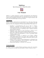
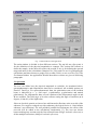
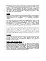
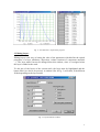
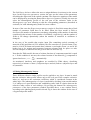
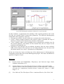
NKDGen
Spectral properties of thin film stacks
User Manual
NKD SOFTWARE, March 2002
Contact: [email protected]
1
NKDGen
Spectral properties of thin film stacks
User Manual
NKDGen is a software application to generate spectrophotometric and ellipsometric
spectra of a thin film stack defined by the user. Generated data can be any of the most
common physical magnitudes measured in a thin films lab. The optical constants of the
layers can be described through a wide range of models.
1. Introduction
NKDGen calculates optical spectra of coated substrates for a wide range of data type
and layer models. The classical electromagnetic theory of light propagation in thin film
stacks [1] is used for the computations. The most important features of the software are:
•
•
•
•
•
•
Simulation of spectrophotometric data for any angle of incidence.
Reflectance, transmittance and backside reflectance, for s-, p- or natural
incident light polarization can be calculated. The backside of the substrate
can be taken into account by considering (single or multiple) incoherent
internal substrate reflections.
Ellipsometric data (∆,Ψ) and related trigonometric quantities can be
simulated to compare with the output of different ellipsometer types.
Wide variety of dispersion models for the materials of the layers (suitable for
dielectrics, metals, and semiconductors), as well as user-defined optical
constants through a text file.
Modellisation of mixtures of materials by the Effective Medium
Approximation (EMA) theory. Our software allows considering more than
two materials in the mixtures [2]. Roughness and interfaces between layers
are also modeled by EMA theory.
Refractive index (n) can have in-deep inhomogeneity, by dividing the layer
in sublayers of equal thickness. The user can define a simple linear profile
for n, a two-slope profile or a segmented profile.
Different units (nanometer, eV, microns, cm-1) can be used.
2. General description
The software consists of a standard Windows application, starting with a presentation
box. Clicking on the Start button, the main window of NKDGen is shown (see Fig.1)
2
Fig. 1 –Main window of the application
The main window is divided in four different sections. The top left one (Spectrum) is
for the definition of the physical magnitude to compute. The section Stack allows to
define the sample. At the down-left corner, the section X-Axis is for defining the spectral
range and units for the calculations. Buttons Plot, Table and File are for performing the
calculations and show them as a graph (Plot), a table (Table) or save as a file (File). The
Exit button finishes the application. Details about these sections are given in following
paragraphs.
2.1 Spectrum
The user can define here the physical magnitude to calculate. As mentioned above,
spectrophotometric and ellipsometric data can be considered. All available options are
listed in DataType. For spectrophotometric data, the polarization state of the incident
beam is indicated by s-, p- and unpol. (s-polarization, p-polarization and natural
polarization). For ellipsometric data, several variations of the ellipsometric angles ∆ and
Ψ are available. The field Angle of incidence allows setting the angle of incidence (φ in
degrees, 0º≤φ<90º) of the light beam.
Substrate backside permits to choose how add internal reflections at the rear-side of the
substrate. For rough or wedged rear-side substrates, the logical choice is ‘Semi-infinite
substrate’ (no reflections). For well polished, parallel faced substrates, the effect of the
rear-side will be added to the calculations incoherently [3]. The user can choose
between taking into account only the first reflected beam (Single backside reflection) or
all the multiple reflections (Multiple backside reflection).
3
Remark: Some restrictions apply for the Data type. For ellipsometric data the substrate
is always considered as semi-infinite and the angle of incidence must not be zero. The
user has to be careful with the multiple options offered by the program, in order to avoid
meaningless optical data calculations. For instance, it is probably meaningless to
consider multiple contributions from the backside when computing the reflectance at 45
deg. incidence angle for comparing with an experimental measurement, as these
contribution will be lost by the detector.
2.2 Stack
In this section the user defines the layers that configure the stack. At the left side the
current structure of the coating is shown, with the layers numbered, from incident to
emergent medium, as 1,2…, S (substrate), … 2’,1’. A maximum of 50 layers is
permitted.
The right side has a set of buttons that allow manipulating layers. The options are: Add
Layer (adding layers, selecting the model), Edit layer (editing the parameters of a
selected layer (see below)), Plot dispersion (plotting the optical constants (n and k) of
the highlighted layer in the range defined in X-Axis), Delete layer (deleting a selected
layer), or Set as substrate (setting a selected layer as substrate). It is possible also to
move the layer position in the stack with the Up and Down buttons.
The user has to note that some restrictions apply to the configuration of the stack.
Roughness layers can only be placed in contact with the incident or emergent media.
Interfaces can not be in contact with a Roughness layer (in fact, roughness is an
interface between the material and air) or with another Interface. One layer must be
defined as substrate, and it must be homogeneous. If any of these conditions is not met,
when one tries to generate data, a message will notify the user which item is not correct.
2.3 X-Axis
This is to define the range for the spectral calculations. Minimum and maximum indicate
the limits, and NumPoints the number of points (equidistant) within the range
(maximum NumPoints is 1000). The user must also define the Units of the spectra
(nanometers, microns, eV or cm-1).
2.4 “Plot”, “Table” and “File” buttons
All these buttons perform the calculation of the optical data selected in section
Spectrum, of the currently defined Stack, in the range indicated in X-Axis. Calculations
are presented in different forms. Pressing the button Plot, a 2-dimensional graph will
appear showing the generated data. Pressing Table, the results will be shown as a table
within a window. If ellipsometric data are generated, two graphs or two tables (∆/Ψ)
will show. These two kind of output are shown in Fig.2. If the button File is pressed, the
data will be calculated and saved into a file in ASCII format.
4
Fig. 2. Plot and Table: output of the program
3. Editing Layers
Editing layers is the way of setting the value of the parameters which define the optical
properties of a layer (thickness, dispersion, volume fractions of component materials
…). The layer model can not be changed from this window, since it is assigned when
the layer is added to the stack.
To edit one of the layers of the current stack, the layer must be highlighted and the
button Edit Layer has to be pressed. A window (like in Fig. 3) will show, with different
fields depending on the layer model.
Fig. 3- Layer Parameter window
5
The field Layer thickness allows the user to assign thickness (in microns) to the current
layer. In the Dispersion parameters section, the user sets the values of the parameters
describing the dispersion of the optical constants. The dispersive equations of the model
can be displayed by pressing the button Show dispersive equations. Finally, the user can
select the inhomogeneity profile of the real part of the refractive index in the
Inhomogeneity type area, allowing to edit the corresponding parameters (described in
section 4) for each inhomogeneity model in a new window.
In most of the cases the Dispersion parameters section is fixed, this means that a fixed
number of parameter fields have to be filled. When the layer model is EMA or
Oscillators the number of parameters can change (depending on the number of materials
considered in the mixture or the number of oscillators, respectively), and the number of
fields to fill change dynamically (when the number of materials or oscillators is
changed).
In the case of the models that require input files containing optical constants of
materials (EMA and Material File models), the files must have a special format. They
must be in ASCII format and contain three columns: wavelength (in nm.), n and k. No
header has to be written and separators between columns must be spaces or tabs.
Several examples of material files are given in the file materials.zip.
Note that for EMA model, the sum of volume fractions of component materials is equal
to 1. If this condition is not met, the volume fraction of last material (fn) component is
ignored and set to f n = 1 − ∑ f i automatically.
i =1.. n −1
As mentioned, interfaces and roughness are modeled by EMA theory, describing
respectively a mixture of three (2 adjacent layers and air) and two (adjacent layer and
air) materials.
4. Editing Inhomogeneity Layers
Three different refractive index profiles can be applied to any layer. It must be noted
that the refractive index profile affects only to the real part of the complex refractive
index (n), and not to the extinction coefficient, which is considered constant in the
whole layer. The inhomogeneity of a layer is modeled by dividing it into an odd number
L of sublayers of equal thickness and establishing some kind of relation between the
refractive index values of each sublayer. By pressing the button Edit inhomogeneity
parameters of the layer parameters window described above, a new window shows,
according to the inhomogeneity model selected. Fig. 4 shows the window for the case of
a Segmented profile model:
6
Fig.4- Edit inhomogeneity parameters window for a segmented profile
In these windows, a graph depicts the meaning of the required parameters and, at the
left side, the required fields to input these parameters. The different inhomogeneity
models that can be applied to a layer are:
• Homogeneous model: refractive index has a constant value in the whole layer.
• Linear: a linear in-depth variation of the refractive index is assumed; the slope of
this linear variation is the characteristic parameter of this model.
• 2-Line: refractive index varies according to two in-depth linear variations (one for
the external sublayers and another for the internal ones; the two slopes are the
parameters defining this case.
• Segmented: each sub-layer has an arbitrary deviation from the mean refractive
index; the deviations of the sub-layers are not independent and, since the sum of all
deviations must be zero, only L-1 parameters are independent.
In the case of Interface layers and when any of the adjacent layers is inhomogeneous,
calculations will not take into account inhomogeneity degree. The same consideration is
applied to Roughness layers.
References
[1]
R.M.A.Azzam and N.M.Bashara, Ellipsometry and Polarized Light, NorthHolland, Amsterdam, 1975
[2]
Salvador Bosch, Josep Ferré-Borrull, Norbert Leinfellner and Adolf Canillas,
Effective dielectric function of mixtures of three or more materials: a numerical
procedure for computations, Surface Science, Volume 453, Issues 1-3, 2000,
Pages 9- 17.
[3]
H.A. McLeod, Thin Film Optical Filters. American-Elsevier, New York, 1969
7