Download Detailed Tutorial Version 3

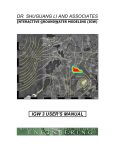
DR. SHUGUANG LI AND ASSOCIATES
INTERACTIVE GROUNDWATER MODELING (IGW)
TUTORIALS
Dr. Shuguang Li and Associates at Michigan State University
IGW Tutorials for Version 3
Copyright © 2002 by Dr. Shuguang Li and Associates at Michigan State University. All
rights reserved.
Dr. Shuguang Li and Associates makes no warranties either express or implied regarding
the program IGW and its fitness for any particular purpose or the validity of the
information contained in this document. The inputs and outputs described herein do not
necessarily represent actual field conditions – they are only used to illustrate the
capabilities of IGW.
Authors:
Kyle Paulson
Dr. Shuguang Li
DOCUMENT VERSION: 2002-4
LAST REVISED: April 9, 2002
http://www.egr.msu.edu/~lishug
0
TABLE OF CONTENTS
CHAPTER 1: INTRODUCTION ______________________________________1
CHAPTER 2: STARTING AND EXPLORING IGW ______________________2
2.1
2.2
2.3
STARTING IGW
GETTING TO KNOW IGW
COMMENTS
2
3
4
CHAPTER 3: SETTING UP A MODEL _______________________________5
3.1
3.2
3.3
3.4
3.5
IMPORTING A BASEMAP
CONCEPTUALIZING THE CROSS-SECTION
DEFINING A ZONE AND ITS ATTRIBUTES
ADDING WATER BODY SOURCES AND SINKS
ADDING A WELL
5
6
7
8
10
CHAPTER 4: OBTAINING A SOLUTION ____________________________11
4.1
4.2
DISCRETIZING THE MODEL
SOLVING THE MODEL
11
11
CHAPTER 5: EXPLORING THE CURSOR ACTIVATED TABLE __________12
5.1
THE CAT
12
CHAPTER 6: EXPLORING THE ATTRIBUTE INPUT AND MODEL EXPLORE
WINDOW __________________________________________13
6.1
THE AIME
13
CHAPTER 7: OPTIMIZING THE DISPLAY ___________________________15
7.1
CHANGING DISPLAY OPTIONS
15
CHAPTER 8: TRACKING PARTICLES ______________________________17
8.1
8.2
8.3
8.4
FORWARD PARTICLE TRACKING
BACKWARD PARTICLE TRACKING
INITIALIZING THE PARTICLES
INITIALIZING THE CLOCK
17
17
17
18
CHAPTER 9: REFINING THE MODEL – DISPERSIVITY ________________19
9.1
ADDING DISPERSIVITY TO THE MODEL
19
CHAPTER 10: MODELING CONTAMINANTS _________________________20
10.1
10.2
10.3
MODELING A CONTINUOUS CONCENTRATION SOURCE
INITIALIZING THE PLUME
INITIALIZING THE CONCENTRATION CLOCK
20
20
20
CHAPTER 11: UTILIZING A MONITORING WELL______________________22
11.1
11.2
11.3
ADDING A MONITORING WELL
OBSERVING THE MONITORING WELL
EXPLORING THE TPS
22
22
23
CHAPTER 12: UTILIZING MASS BALANCES _________________________24
12.1
12.2
SETTING UP AN AREA FOR MASS BALANCE
OBSERVING THE MASS BALANCE
24
24
1
CHAPTER 13: VIEWING CROSS-SECTIONS _________________________25
13.1
DEFINING AND VIEWING THE DESIRED PROFILE VIEW
25
CHAPTER 14: REFINING THE MODEL – STRATIGRAPHY ______________27
14.1
REFINING THE STRATIGRAPHY
27
CHAPTER 15: SUBMODELING ____________________________________ 29
15.1
15.2
ADDING, SOLVING, AND EXPLORING A SUBMODEL
DELETING PROFILE MODELS AND SUBMODELS
29
29
CHAPTER 16: MODELING MULTIPLE SCENARIOS____________________31
16.1
SETTING UP MULTIPLE MODELS
31
CHAPTER 17: SIMULATING TRANSIENT CONDITIONS ________________33
17.1
CHANGING SIMULATION TIME PARAMETERS AND SOLVING
33
CHAPTER 18: STOCHASTIC MODELING ____________________________35
18.1
18.2
18.3
18.4
18.5
18.6
ADDING HETEROGENEITY TO THE AQUIFER
SETTING UP MONTE CARLO STOCHASTIC MODELING
SETTING UP TO MONITOR MONTE CARLO SIMULATIONS
OPTIMIZING THE DISPLAY FOR MONTE CARLO SIMULATIONS
RUNNING THE MONTE CARLO SIMULATIONS
VIEWING MONITORING WELL GRAPHICS
35
35
36
37
37
37
CHAPTER 19: UTILIZING GRAPHICS OPTIONS_______________________38
19.1
19.2
SAVING THE MODEL
SAVING THE DISPLAY AS A PICTURE
38
38
CHAPTER 20: CONCLUSION ______________________________________39
CHAPTER 1: INTRODUCTION
This tutorial is designed to step you through some of the basic features of the IGW software. This tutorial
is designed to be used with version 3 of the software.
You will get the most out of this tutorial if you work the sections sequentially and complete all of the
sections within a chapter at the same sitting. It is recommended that you use the suggested values for each
step in the tutorial. [The suggested values and other appropriate comments appear in bracketed blue text.]
Using the suggested values will walk you through a calibrated, real-world example thus providing results
that are intuitive and instructional.
You should consult the IGW User’s Manual for more in-depth information concerning program
implementation and function.
For detailed information concerning technical content of the model (i.e., mathematics and theory) please
consult the IGW Reference Manual (not yet available as of 4/9/2002).
2
CHAPTER 2: STARTING AND EXPLORING IGW
This chapter will show you how to start the software and will give you an overview of the
software interface. If you are using the hypertext version of the help file then you have already
started the software and you may continue to Section 2.2.
2.1
STARTING IGW
The easiest way to start the program is to use the Windows™ Start menu.
Step 1: Click on the Start button, open the Programs sub-menu, then the Interactive
Groundwater sub-menu, and then select IGW 3.x (This assumes the software has
been installed correctly.)
You will see a splash screen with the software credits. You can either wait 15 seconds for the
screen to expire or click on the ‘Press to continue’ button.
A full-screen IGW window appears. See Figure 2.1.1.
FIGURE 2.1.1
Main window for IGW 3
3
2.2
GETTING TO KNOW IGW
The first thing you notice is the ‘Tip of the Day’ Window. This window gives you a new tip every
time you start the software. If you want to disable this function, deselect the ‘Show tips as startup’
box before closing the window. You can also access the Frequently Asked Questions file, access
the hypertext version of the tutorial, or open the Help file by clicking the appropriate button in this
window.
You may also access the Help file at any time by selecting ‘Help content’ from the ‘Help’ menu
on the main screen menu bar.
Step 1: Click the ‘Close’ button when you are finished with the ‘Tip of the day’ window.
The entire Main Window is now completely visible. The upper left-hand portion of the window is
a button palette. This palette provides you with one-click access to the most commonly used
features in IGW.
Step 2: Place the cursor over the upper-most, left-most button.
A bubble-box briefly appears near the cursor with the words ‘Create a New Model’ in it. This
bubble-box is informing you as to the functionality of the button. Bubble-boxes are available for
all active buttons on the palette.
Step 3: Click on the ‘Help’ button.
The cursor is now initialized to provide help with any button on the palette.
appears as part of the cursor, next to the arrow.)
(A question mark
Step 4: Click on any button.
A help window appears. It provides an explanation of the selected button’s functionality.
Step 5: Close the help window when finished.
Step 6: Bring the cursor out of help mode by clicking on the ‘Reset toolbar
buttons state’ button. Use this button at any time to reset the cursor.
For more in-depth explanation of button functions and subsequent implementation, refer to the
IGW User’s Manual.
The remainder of the left-hand portion of the window is the ‘Step Adjustment and Time Display
Interface’ (SATDI). The SATDI provides you with quick access to computational and display
adjustments. The time step (DT) (10 by default) can be adjusted using the up/down buttons next
to the units list field (day by default). The plume step, particle step, and visual step can be set in a
similar fashion, as a ratio of the DT. (These parameters can also be set by clicking the ‘Set
Simulation Time Parameters’ button. This is discussed more in Chapter 11.) The Flow Time,
Plume Time, and Particle Time sections display the computational time for the flow, plume, and
particles, respectively. By clicking anywhere in the SATDI and then pressing F1, you can access
a more in-depth explanation of the SATDI features.
The major portion of the right-hand side of the window is occupied by what is known as the
‘Cursor Activated Table’ (CAT). This table will display the variable values that exist in the model
4
at any point the cursor is located. It is more intuitive to explore the CAT with a working model,
so this discussion is expanded in Chapter 5.
The middle of the main window is occupied by the ‘Model Screen’. The white rectangle within
the Model Screen is referred to as the ‘Working Area’. This is where you define features, assign
attributes, and obtain solutions. The peach colored rectangle below the Working Area is referred
to as the ‘Working Area Attribute Display’ (WAAD). The WAAD displays information
concerning the flow solution and the elapsed time in the solution for each Working Area within
the Model Screen. You may click in the WAAD and subsequently type in your preferred title for
the present model state.
The upper right portion of the main window is called the ‘Time Process Selector’ (TPS). From
this section, you can open a separate window for any previously defined time process (mass
balance, mass flux, well head, well concentration, etc.) and view the results as the model solution
iterates. Again, it is more intuitive to explore TPS functionality with a working model, so the TPS
discussion is continued in Section 11.3.
2.3
COMMENTS
This chapter was designed to give you a brief overview of the IGW interface and help options.
You now have the basic skills to complete the rest of the tutorial sections. While we have not
explored the functionality in depth, one of the powerful features of IGW is that it is very intuitive.
That intuitive quality helps you grasp the functionality from the logical layout of the software and
the interface. Thus, we will rely on the intuitive nature to help you understand the functionality
better.
The following chapters will employ that intuitive quality in a series of directed steps that will
culminate in a solution to a real-world problem. When finished, you will have solved a complex
groundwater contamination problem with software you have only begun to use!
CHAPTER 3: SETTING UP A MODEL
This chapter will walk you through the basic procedures for setting up a model in IGW.
3.1
IMPORTING A BASEMAP
Intuitively, the first step in defining a model is to know its associated real-world characteristics. Let us
begin with the plan view location.
Most of the work in defining model features will be done in the Working Area, so let us first import a
picture to use as a basemap in defining our model features.
Step 1: Select the ‘Set Basemap and Register a Basemap’ button.
This brings up the ‘Model Scale and Basemap’ window.
Step 2: Click the ‘Load Basemap’ button.
5
This brings up the ‘Open’ window. Browse to the location that your basemap is located. Currently, IGW
supports BMP, GIF, JPG, SHP and DXF file types. [The suggested basemap is located at x:\Program
Files\Interactive Groundwater y.z\doc\tutorial.bmp (where x is the drive that IGW is installed on and y.z
corresponds to the version number). A picture of the basemap can be seen in Figure S3.1.1: Suggested
Tutorial Basemap.]
FIGURE S3.1.1
Suggested tutorial basemap
If you open a BMP, GIF, or JPEG file, the ‘Vectorization of Raster Pictures’ window appears (go to Step
3). If you open a SHP or DXF file, proceed with the tutorial immediately following Step 4 (these files do
not need to be vectorized).
Step 3: Set the origin coordinates and the image lengths corresponding to the real world. At a
minimum, you should set the XLength [6800 ft] as the horizontal distance that the
basemap covers in the real world. (Note: First change the units and then input the
numerical value. When you change units, IGW automatically converts the existing
numerical value into the new units. Getting in this habit will prevent input errors when
inputting data into IGW. Also, after changing units, be sure to delete all numbers from
the numerical field. Some numbers may be present in the field, but not visible, due to the
number having many decimal places. Again, this helps prevent data errors.) The
YLength will self-calculate based upon the dimensions of the image. XO and YO are
coordinates for the left, bottom most corner of the picture. These are set to zero as the
default [use the default values].
Step 4: Click ‘OK’.
6
The ‘Model Scale and Basemap’ window becomes visible again with the selected basemap as a preview.
Here you can also make adjustments to the scale and coordinates for the files. (Note: If you change the
YLength value the picture does not distort, but the working does display the extra space as white area.)
Step 5: Click ‘OK’.
The program returns to the main screen with the desired basemap as the background in the Working Area.
IGW also allows you to bring in multiple files of mixed formats. Simply repeat the steps above to bring in
another file and it automatically merges with the present basemap. This means that the pictures are both
visible and scaled but now become one image in the software. Consequently, if you import an incorrect
picture or assign the wrong scale, you will have to clear the entire merged basemap set.
With the basemap set, you can now define areas and features that correspond to the map you have
imported.
3.2
CONCEPTUALIZING THE CROSS-SECTION
This is not an IGW function per se, but as with all modeling we must have an understanding of the
geological composition of the model site.
[The cross-section A-A′ associated with Figure S3.1.1 can be seen in Figure S3.2.1: A-A′ Cross-section.]
At a minimum, we would like to know the aquifer properties (top and bottom elevations, hydraulic
conductivity) and the existence of sources and sinks (and associated characteristics).
[From Figure S3.2.1 we are given layer elevations, some layer properties, and source and sink properties.
Notice also the General Regional Flow direction. This will help us determine the extent of our model.]
This information allows us to accurately model the aquifer of interest. [In this case, we are modeling the
‘Sandstone Aquifer’ as seen in Figure S3.2.1.]
7
A
A′
FIGURE S3.2.1
A-A′ Cross-section (not to scale)
3.3
DEFINING A ZONE AND ITS ATTRIBUTES
A good place to start in building a model is to define the zone over which the solution will apply. We want
to define the boundaries at places where water does not flow through said boundaries or where the head is
known. [In this case we can use the entire plan view as the model area as the north boundary is a constant
head due to the river, the south boundary is a no flow boundary because the aquifer pinches off and the east
and west boundaries are no flow boundaries because of the regional flow direction.]
Once you have determined your boundaries you can proceed to Step 1.
Step 1: Click the ‘Create New Arbitrary Zone as Assign Property’ button.
The cursor is now initialized to add zones in the working area.
Step 2: Create a zone that corresponds to your pre-determined boundaries [the entire working
area]. A zone is created by selecting points cyclically around the area you wish to
enclose as the zone. Click the mouse at a location on the zone boundary. Move to
another location and repeat. When you have finished, double-click the mouse. (Note:
You can easily define a rectangle by holding down the shift key before clicking the
mouse on the first point and then simply moving the cursor to the opposite end of the
rectangle and clicking the mouse again.)
A zone is now defined that covers the entire area of the model screen. This zone will be referred to as the
‘parent zone’. The edges of the zone will now appear red in the model screen. This indicates that the zone
is currently being accessed.
8
Step 3: Assign attributes for the newly defined zone. Hit the ‘ctrl’ key to toggle to the ‘Attribute
Input and Model Explore’ window (AIME). Alternately, drag the window from the
lower right-hand corner of the Windows™ screen and into the middle. (The ‘ctrl’ key
toggling action will occasionally become disabled if you are accessing other windows
programs while using IGW. To re-enable the ‘ctrl’ toggling option simply select ‘Show
model explore window’ from the Display menu.) Also, you can right-click on the AIME
title bar and select ‘Move Form Quickly’ from the subsequent menu to toggle the
location. (Note: If you are using a two-monitor system, it is very useful to put the AIME
on the second display.) The AIME is explained in greater detail in the IGW User’s
Manual and is explored more in Chapter 6.
Notice that the zone is highlighted in the left-hand pane. This corresponds to the edges of the zone being in
red in the working area; it is currently being accessed.
a)
b)
c)
d)
e)
f)
g)
h)
i)
j)
k)
Select the ‘Conductivity’ box (on the ‘Physi/Chemical Properties’ layer of the
right-hand side pane). Change the units to the desired units [m/day]. Enter a value
[30]. (Note: when you select a box, you can press F1 to get a list of typical
values.)
Select the ‘Porosity’ box. Enter a value [.2].
Click the ‘Aquifer Type / Elevations’ tab to get to that layer of the right-hand
pane.
Select the ‘Surface Elevation’ box and enter a value* [10]. As always, be sure to
adjust units prior to entering the desired value. (Note: If you use the default values
you do not have to re-type them.)
Select the ‘Top Elevation’ box and enter a value [-10].
Select the ‘Bottom Elevation’ box and enter a value [-50].
Click the ‘Sources and Sinks’ tab.
Select the ‘Const Rech’ (Constant Recharge) box.
Change to the desired units. [inch/year].
Enter a value [10].
Click the ‘Apply’ button. Remember to click this button after entering any new
values.
[At this point feel free to explore the AIME but do not enter any more values, as you have not been
provided with enough information.] Steps 3a-3h were designed, in part, to show you how to input
characteristics for model features. You may now move the AIME out of the way of the main window to
make it easier to continue work on the model.
* The surface elevation is not trivial. It is important in unconfined aquifer situations where the top
elevation is set equal to the surface elevation, in viewing the stratigraphy in a cross-section, and in
determining the value of some other parameters (such as leakances).
3.4
ADDING WATER BODY SOURCES AND SINKS
Next we will focus on adding water body type sources and sinks to the model.
Step 1: Click the ‘Create New Arbitrary Zone and Assign Property’ button (you will not
need to click it if it is still selected from previous use).
The cursor is now initialized to add zones in the Working Area.
Step 2: In the Working Area, click the pointer on any edge of the feature [Columbia River] you
wish to define. (If you are not using a basemap, simply click anywhere to begin defining
9
an arbitrary feature.) Click the mouse at another location on the edge of the feature.
Move to another location and repeat. When you have finished, double-click the mouse.
Try to keep the lines as close to coinciding with the edge of the feature as possible.
Step 3: Access the AIME to assign attributes for the newly defined zone. (Refer to Section 3.3 –
Step 3 for instructions on accessing the AIME.)
a) Click the ‘Sources and Sinks’ tab.
b) Select the type of water body that you would like to model: River, Prescribed
Head, or Drain. [Model the Columbia River as a Prescribed Head water body by
selecting ‘Constant Head’ in the ‘Prescribed Head’ area.] Consult the IGW User’s
Manual for explanations of the types.
(Note: If defining a Prescribed Head feature you will need to select ‘Const Rech’
and enter a value of 0 if the feature is located in a larger zone that has a non-zero
recharge value. This is because the Prescribed Head feature already accounts for
any recharge in the area. This is done automatically for other water bodies.) [Do
this.]
c)
Enter a value for the stage, elevation, or head of the feature (you may need to
activate the field by first selecting its parent area). [3 in the ‘Constant Value’
field in the ‘Constant Head’ area (in the ‘Prescribed Head’ area)]
d) Click the ‘Apply’ button.
Step 4: Repeat Section 3.4 for other features you wish to define. [Follow the steps below.]
[Step 5: In the Working Area, click the pointer on any edge of the northern lake (refer to it as
‘North Lake’). Click the mouse at another location on the edge of North Lake. Move to
another location and repeat. When you have finished, double-click the mouse.
Step 6: Access the AIME to assign attributes for North Lake.
a)
b)
c)
d)
Click the ‘Sources and Sinks’ tab.
Model North Lake as a River water body by selecting the ‘River’ box.
Enter 3 in the ‘Constant’ field in the ‘Stage’ area (in the ‘River’ area).
Click the ‘Sediment Properties…’ box in the ‘Leakance’ area (in the ‘River area).
The ‘River Bottom Sediment Prop…’ window appears.
e)
f)
Change the ‘Sediment cond K’ units to ft/day and change the value to 0.1.
Click the ‘OK’ button.
The ‘River Bottom Sediment Prop…’ window closes.
g) Enter –2 in the ‘Constant’ field in the ‘River Bottom’ area (in the ‘River’ area).
h) Click the ‘Apply’ button.
Step 7: In the Working Area, click the pointer on any edge of the southern lake (refer to it as
‘South Lake’). Click the mouse at another location on the edge of South Lake. Move to
another location and repeat. When you have finished, double-click the mouse.
Step 8: Repeat Step 6 for South Lake using 3.5 for the stage and 0 for the river bottom. ]
10
3.5
ADDING A WELL
A well is simply another type of source or sink. The following steps illustrate how to add a pumping well
to the model.
Step 1: Click the ‘Add a New Well’ button.
The cursor is now initialized to add well features to the model.
Step 2: Select a point in the model where a well might be located and click the mouse at that
point. [Add a well at the circle between North and South Lake.]
A well feature now appears at that point.
Step 3: Access the AIME to assign attributes for the newly defined well.
a)
b)
c)
d)
e)
f)
Make sure that ‘Pumping Well’ is selected in the ‘Well Type’ area.
In the ‘Flow Rate’ area, select ‘Constant Q’.
Change the unit field menu to the desired units [GPM (gallons per minute)]
Enter a value in the ‘Constant Q’ field. [-80] Negative values indicate water
being withdrawn from the well.
Enter a new name in the ‘Well Name’ field. [Middle Well]
Click the ‘Apply’ button.
[Repeat Step 2 and Step 3 for the circle to the right of North Lake. Use the same values. Name it ‘East
Well’.]
CHAPTER 4: OBTAINING A SOLUTION
This chapter will walk you through the basic procedures for solving a model in IGW.
4.1
DISCRETIZING THE MODEL
Discretizing the model turns the conceptual model into a numerical model that the computer will solve.
Step 1: Click the ‘Convert the Model into a Numerical Model’ button to discretize the
model.
This sets up a default grid (not visible by default) that covers the working area. The grid size is determined
by taking a default value of sections in the x-direction (40) and then determining the number of sections in
the y-direction based on the dimensions of the Working Area and the condition that the cells resulting from
the sectioning be as close to square as possible.
In some cases, you may want to set a specific grid size or grid characteristic.
Step 2: Click the ‘Set Simulation Grid’ button.
This brings up the ‘Grid Option’ window. Here you may enter the number of sections in the x-direction
(NX). The computer calculates the number of section in the y-direction (NY)*, and the cell dimensions DX
11
and DY based on this number and the dimensions of the Working Area (‘X Length’ and ‘Y Length’). A
higher grid resolution yields a more accurate solution but increases computational time. The grid
resolution is left to you, as it is very dependent on the problem being solved and the speed of the computer
being used to solve it.
Step 3: If you do not want to change the grid then click ‘Cancel’. To keep any updated settings,
click ‘Discretize/OK’.
The model is now ready to solve.
* The user may subsequently change the NY value (without affecting NX) to deform the cells from their
default square shape into an arbitrarily assigned rectangle shape. (There is a bug in the implementation of
this feature that is currently being addressed by the software engineers.)
4.2
SOLVING THE MODEL
Once the numerical model is set the next logical step is to solve it. Continue only after you have
discretized your conceptual model.
Step 1: Click the ‘Forward’ button.
By default, the model is solved at steady state. The model screen will now display the head contours and
velocity vectors.
[It may not appear that the small lakes are having any effect, but we will show you in a later section how
you can check the extent of their influence.]
CHAPTER 5: EXPLORING THE CURSOR ACTIVATED TABLE
This short chapter introduces you to the Cursor Activate Table (CAT) first mentioned in Section 2.2.
5.1
THE CAT
As mentioned earlier, the CAT occupies the major portion of the right hand side of the main window. If
you move the cursor around the working area, you will notice the values in the CAT change to display
those particular values that exist at the location in the model.
The values you see in the CAT are set by default. Step 1 shows you how to change them.
Step 1: Click on the ‘Choose Parameters at Cursor’ button.
The ‘Choose Parameters at Cursor’ window appears. From here you can select which parameters you
would like displayed in the CAT. The parameters are also defined in this window. This is useful as the
field names displayed in the CAT are truncated.
Step 2: Click the ‘OK’ button to close the window.
12
You can also change the units for particular variables. This is accomplished by selecting the arrow
corresponding to the unit field you would like to modify then simply selecting the desired units from the
drop-down list. IGW now displays these units.
Also, there may be more variables in the CAT than are visible at a particular time. To view the hidden
variables, simply use the scroll bar on the far right to access them.
CHAPTER 6: EXPLORING THE ATTRIBUTE INPUT AND
MODEL EXPLORE WINDOW
This short chapter will introduce in greater detail to the Attribute Input and Model Explorer window
(AIME).
6.1
THE AIME
You have been using the AIME to input values for the features that you have defined in the previous
chapters. The steps below guide you through some extra features of the AIME that have not been
completely explained.
Step 1: Bring the AIME to a visible location.
You will notice that there are two panes. The left-hand pane (Model Explore pane) is a hierarchical
visualization of the model. The right-hand pane (Attribute Input pane) is where attributes are entered for
the features of the model.
There is also a second layer to AIME that is tabbed with the title ‘Data Table’. (This layer is not yet
functional in IGW). Also notice the ‘Apply’ button. You should get in the habit of clicking this button
every time you input new values into the AIME.
The parent field in the Model Explore pane is titled ‘Project’
Step 2: Click on ‘Project’.
The Attribute Input pane now changes to display general project attributes.
Step 3: Enter desired information.
Step 4: Click the ‘Apply’ button.
Step 5: Click on ‘Model’ in the Model Explore pane. The Attribute Input pane now displays a
collection of buttons (also available on the button palette) that can be selected to alter
attributes for the model. Multiple models are discussed more in Chapter 14.
Step 6: Click on ‘Layer1’ in the Model Explore pane. The fields that appear in are not operational
as IGW 3 is a one-layer version and the layer attributes are determined by the aquifer
definitions.
Step 7: Click on ‘Zones’ in the Model Explore pane.
13
Nothing appears in the Attribute Input pane. This is merely a placeholder in the Model Explore hierarchy.
All attributes for the zones need to be set individually.
Step 8: Click on one of the zones that is in the ‘Zones’ group. The Attribute Input pane now
displays a multi-layered section for entering information about this particular zone.
Notice this is where you entered data for the water body sources and sinks you defined in
previous sections.
The Attribute Input pane will be available and will be different for every type of feature that you can define
in IGW including (but not limited to): wells, particle zones, profile models, sub-models, and line features.
As you work through the tutorial keep an eye on the AIME and take notice of the new features that become
available as your model increases in complexity.
Also, you can right-click on the features and groups in the Model Explore pane and perform such functions
as deleting them*, viewing attributes, and reading in scatter points (discussed later).
* It is more reliable to delete items by highlighting them in the Working Area and pressing the ‘Delete’ key.
(There is a bug in the software that sometimes will not let you delete items from within the AIME. The
software engineers are investigating this problem.)
CHAPTER 7: OPTIMIZING THE DISPLAY
This chapter will walk you through the basic procedures for optimizing the working area display.
7.1
CHANGING DISPLAY OPTIONS
Some features may be difficult to discern, especially with a basemap in the screen. The following steps
show you how to change display options in the model screen.
Step 1: Click the ‘Set Drawing Options’ button.
The ‘Draw Option’ window appears.
Step 2: In the ‘Flow and Transport Visualization’ area, click the ‘…’ button to the right of ‘Head’.
The ‘Draw Option -- Head’ window appears.
Step 3: Click the ‘Color…’ button.
The ‘Color’ window is now open.
Step 4: Click on a yellow color (or any other that you feel will be effective) then click ‘OK’.
You return to the ‘Draw Option -- Head’ window and you can see that the color is now set to yellow (or
your chosen color).
Step 5: Enter 2 (or any other that you feel will be effective) in the ‘Thickness’ field.
Step 6: Click ‘OK’
14
You return to the ‘Draw Option’ window.
Step 7: In the ‘Flow and Transport Visualization’ area, click the ‘…’ button to the right of
‘Velocity’.
The ‘Velocity Draw Option’ window appears.
Step 8: Click the ‘Color…’ button.
The ‘Color’ window is now open.
Step 9: Click a blue color (or any other that you feel will be effective) then click ‘OK’.
You return to the ‘Velocity Draw Option’ window.
Step 10: Click the ‘OK’ button.
You return to the ‘Draw Option’ window. Notice the ‘Set Visualization Sequence (top to bottom)’ area.
This area shows the order of display for the model screen. In some cases it may be helpful to adjust these
settings or to remove non-essential elements. It is left to you to experiment with these settings.
Step 11: Click the ‘OK’ button.
You return to the model screen and the drawing updates have taken effect. If the settings
have not taken effect, simply click the refresh button.
CHAPTER 8: PARTICLE TRACKING
This chapter will show you how to track some particles in the model.
8.1
FORWARD PARTICLE TRACKING
The following steps will show how to track a collection of discrete particles.
Step 1: Click the ‘Add Particles Inside a Polygon’ button.
The cursor is now initialized to add particles.
Step 2: Trace some areas [Boeing and Cascade] (using the same methodology as in Section 3.4) to
define contamination plumes. For each area defined you will be prompted with the
‘Particles’ window. Here you should define how many columns of particles you want to
include in your area (number proportional to concentration). Enter the number in the
field and click the ‘OK’ button.
Your contamination fields are now defined in the model screen.
Step 3: Click the ‘Forward’ button to solve the model. (Note: Unlike all other model
features, you do not need to discretize the model after adding particle features.)
15
Notice now that with the particles present, the model solution now continuously updates at the time step
indicated at the lower left of the main screen. You may need to adjust this time step to see any significant
changes from one time-step to the next. You may speed up the simulation by changing the Visual Step to a
higher number. This instructs the software to redraw the simulation at fewer time-steps. These variables
are highly dependent on the problem being solved and the speed / capacity of the computer running the
simulation, therefore, this tutorial leaves it to the reader to optimize these values. [Setting DT to 80 and
using a visual step of 4 DT will give you good visualization results.]
Step 4: Stop the simulation by clicking the ‘Stop’ button.
8.2
BACKWARD PARTICLE TRACKING
The following steps show you how to backward track a plume of contaminants. This is useful if you are
trying to determine where some pollution came from.
Step 1: Click the ‘Reverse’ button.
Watch the particles moving backwards and the time elapsed clock counting towards zero and going into the
negative numbers.
Step 2: Stop the simulation by clicking the ‘Stop’ button.
8.3
INITIALIZING THE PARTICLES
Step 1: Click the ‘Initializing Particles’ button to return the particles to their initial
location.
8.4
INITIALIZING THE CLOCK
Step 1: Click the ‘Reset Particle Clock’ button to reset the clock.
The time elapsed clock in the Working Area Attribute Display (WAAD) returns to 0 days.
CHAPTER 9: REFINING THE MODEL - DISPERSIVITY
This chapter shows you how to perform particle tracking in the presence of dispersivity.
9.1
ADDING DISPERSIVITY TO THE MODEL
The following steps walk you through adding dispersivity to the model and viewing the results in terms of
the particle paths.
Step 1: In the Attribute Input and Model Explore window (AIME), access the parent zone (the one
that encompasses the entire area over which the model solution applies).
16
Step 2: Select the ‘Local Dispersivity’ box on the ‘Physi/Chemical Properties’ layer in the
Attribute Input pane.
Step 3: Enter values for the longitudinal (Long.) [5] and transverse (Trans.) [1] dispersivities.
Step 4: Click the ‘Apply’ button.
Step 5: Click the ‘Convert the Model into a Numerical Model’ button to discretize the
model.
Step 6: Click the ‘Forward’ button to solve the model.
Notice any differences in the particle movement that changing the dispersivity values has caused.
Step 7: Stop the simulation by clicking the ‘Stop’ button.
Step 8: Click the ‘Initializing Particles’ button to return the particles to their initial
location.
Step 9: Click the ‘Reset Particle Clock’ button to reset the clock.
CHAPTER 10: MODELING CONCENTRATION PLUME
MIGRATION
Instead of modeling contaminants as particles, we can model them as a plume. The following sections will
help you set up a contamination plume.
10.1
MODELING A CONTINUOUS CONCENTRATION SOURCE
The following steps show you how to set up a continuous concentration source in the model.
Step 1: Create a new zone where contamination might be located [Autoshop] using
the ‘Create new zone and assign property’ button.
Step 2: Access the newly created zone in the Attribute Input and Model Explore window (AIME).
Step 3: Click on the ‘Sources and Sinks’ tab in the right-hand side pane to get to that layer.
Step 4: In the ‘Source Concentration’ area, select the ‘Const Conc.’ (Constant Concentration) box.
Step 5: Enter a value in the ‘Const Conc.’ field. [100 ppm]
Step 6: Click the ‘Apply’ button.
Solutions for concentration plumes are very dependent on the grid size and the time step. They may
become unstable at too coarse a grid resolution or too large a time step. You should increase the resolution
of the grid and/or decrease the time step if your solution does in fact become unstable.
17
Step 7: Click the ‘Convert the Model into a numerical model’ button to discretize the
model.
Notice a plume appears inside the newly defined zone.
Step 8: Click the ‘Forward’ button to solve the model.
Notice how the plume spreads from the source. Also notice that you can model particles (the ones added in
Chapter 8) and plumes simultaneously.
Step 9: Stop the simulation by clicking the ‘Stop’ button.
10.2
INITIALIZING THE PLUME
Step 1: Click the ‘Initializing Plume’ button. (If at anytime this does not do
anything then you will need to discretize the model.)
The plume returns to its original location.
10.3
INITIALIZING THE CONCENTRATION CLOCK
Step 1: Click the ‘Reset Conc Clock’ button.
The time elapsed clock at the bottom of the main screen returns to 0 days. If not, you have to
initialize the flow clock and/or the particle clock.
You must also separately initialize any particles (such as those added in Chapter 8) and reset the clock
with respect to them.
Step 2: Click the ‘Initializing Particles’ button to return the particles to their initial
location.
Step 3: Click the ‘Reset Particle Clock’ button.
CHAPTER 11: UTILIZING A MONITORING WELL
This chapter shows you how to add and observe a monitoring well.
11.1
ADDING A MONITORING WELL
Monitoring wells are useful to examine the concentration of a contaminant at a point of interest.
Step 1: Click the ‘Add Well’ button.
The cursor is now initialized to add wells in the model screen.
18
Step 2: Place the cursor downstream of the plume (created in Chapter 10) [to the right of South
Lake] and click the mouse button.
Step 3: Access the newly defined well in the Attribute Input and Model Explore window (AIME).
Step 4: In the ‘Well Type’ area, select ‘Monitoring Well’ (it is in disabled text by default).
Step 5: Type ‘Monitoring Well’ in the ‘Well Name’ field.
Step 6: Click the ‘Apply’ button.
Step 7: Click the ‘Convert the Model into a Numerical Model’ button to discretize the
model.
11.2
OBSERVING THE MONITORING WELL
You could tell by watching the simulation whether or not the plume passes through the monitoring well.
However, it is much more useful to observe the concentrations experienced in the observation well.
Step 1: In the Time Process Selector (TPS), located in the upper-right hand corner of the Main
Window, double-click on ‘Time Process’ under ‘Monitoring Well’.
This opens up a window entitled ‘Time Process at Monitoring Well’.
Step 2: Select ‘Concentration’.
Step 3: Click the ‘Forward’ button to solve the model.
You can now view the concentration in the monitoring well as the simulation runs.
Step 4: Click the ‘Stop’ button to solve the model.
You may close the window at any time after stopping the simulation.
Step 5: Click the ‘Initializing Plume’ button to initialize the plume.
Step 6: Click the ‘Reset Conc Clock’ button to reset the clock.
You must also separately initialize any particles (such as those added in Chapter 8) and reset
the clock with respect to them.
Step 7: Click the ‘Initializing Particles’ button to return the particles to their initial
location.
Step 8: Click the ‘Reset Particle Clock’ button.
11.3
EXPLORING THE TIME PROCESS SELECTOR
The TPS allows you to access any monitoring processes or features that you have defined in the AIME.
When you first discretize the model, three fields appear in the TPS. One is for wells, one for polylines, and
one for zones. Anytime you define a monitoring process for a feature in the AIME and then discretize the
model, you will be able to access that process in the TPS by double-clicking on it. All monitoring
processes are viewed in their own window.
19
CHAPTER 12: UTILIZING MASS BALANCES
It is often intuitive to understand the relationship between influxes and out fluxes for water or contaminants
for a given area of interest.
12.1
SETTING UP AN AREA FOR MASS BALANCE
It is often revealing to examine the mass balance for the entire active model area.
Step 1: In the Attribute Input and Model Explore window (AIME), access the parent zone.
Step 2: In the lower right-hand corner of the Attribute Input pane, check the box for ‘Perform
Mass Balance’.
Step 3: Click the ‘Apply’ button.
Step 4: Click the ‘Convert the Model into a Numerical Model’ button to discretize the
model.
12.2
OBSERVING THE MASS BALANCE
Step 1: In the Time Process Selector (TPS), double-click on ‘Water Balance’ and ‘Plume Mass
Balance’ for the zone used in Section 12.1.
Two windows will appear.
Step 2: Click the ‘Forward’ button to solve the model.
Watch the graphical representation of the mass balances. In the ‘Water Balance’ window, notice the flux
associated with ‘River’. This is the amount of water contributed from both North Lake and South Lake.
So, as mentioned alluded to in Section 4.2, although you cannot visibly see the contributions of these lakes,
you can assess their impact through other IGW features.
Step 3: Click the ‘Stop’ button to stop the simulation.
You may close the windows at any time after stopping the simulation.
Step 4: Click the ‘Initializing Plume’ button to initialize the plume.
Step 5: Click the ‘Reset Conc Clock’ button to reset the clock.
You must also separately initialize any particles (such as those added in Chapter 8) and reset
the clock with respect to them.
Step 7: Click the ‘Initializing Particles’ button to return the particles to their initial
location.
20
Step 8: Click the ‘Reset Particle Clock’ button.
CHAPTER 13: VIEWING CROSS-SECTIONS
This chapter shows you how to view cross sections and explains some of their attributes.
13.1
DEFINING AND VIEWING THE DESIRED PROFILE VIEW
Step 1: Click the ‘Define a Profile Model’ button.
The cursor is now initialized to add a profile model in the working area.
Step 2: Click on a point where you would like to begin your profile view. [On the pre-defined
cross-sectional view near the A.]
Step 3: Drag the cursor to the point where you would like to stop your profile view and doubleclick the mouse. [On the pre-defined cross-sectional view near the A′.]
A window appears titled ‘Profile Model X’ (where X is a number pre-determined by the IGW software).
Step 4: Click the ‘Convert the Model into a Numerical Model’ button to discretize the
model.
Step 5: Click the ‘Forward’ button to solve the model.
You will now see a cross-sectional view that includes the stratigraphy, the velocity profile, a continuous
head representation, and any model features that the cross-section intercepts (not including particles or
contaminant plumes).
Step 6: Click the ‘Stop’ button to stop the simulation.
You must separately initialize any particles (such as those added in Chapter 8) and any plumes (such as
the one defined in Chapter 10) and reset the clock with respect to them.
Step 7: Click the ‘Initializing Plume’ button to initialize the plume.
Step 8: Click the ‘Reset Conc Clock’ button to reset the clock.
Step 9: Click the ‘Initializing Particles’ button to return the particles to their initial
location.
Step 10: Click the ‘Reset Particle Clock’ button.
Next we want to close the profile model window.
Step 7: Close the ‘Profile Model X’ window.
This turns off visualization of the profile model but does not delete it altogether. This allows you to get the
best view of the working area and maximize computational power while allowing you to re-open the profile
model at a later time.
21
IGW allows you to formulate profile models that do not follow the grid orientation. Also, IGW treats
cross-sections in such a way that they do not have to be drawn along streamlines. The profile view, in IGW
3, is an actual model in and of itself and when representing the cross-section, any net cross-flow into the
profile slice is treated as recharge for the profile model, thus maintaining an accurate representation.
Profile models can also be viewed in a non-linear fashion. Instead of double-clicking on the second point
when defining a profile model, simply keep defining the cross-section (by single clicking on points) in any
desired direction. Now when you solve the model this entire defined section is projected into a twodimensional window and appears as a simple cross-section. Currently, IGW does not indicate any threedimensional attributes in the profile model window; so if you define a complex cross-section keep in mind
what it is you are actually viewing.
CHAPTER 14: REFINING THE MODEL – STRATIGRAPHY
14.1
REFINING THE STRATIGRAPHY
These steps take you through the process of adding scatter points. Scatter points allow us to add
complexity to the model as they are points where specific physical characteristics are know about the
aquifer (or other features).
The zone you want to add scatter points to must be selected before adding them.
Step 1: Click the ‘Select a Zone’ button.
The cursor is now initialized to select a zone.
Step 2: Click the mouse inside the parent zone (but not inside any other zone).
The parent zone appears with red borders in the Working Area indicating that it is active.
Step 3: Click the ‘Add Scatter Point’ button.
The cursor is now initialized to add scatter points into the selected zone. (Note: even if you placed scatter
points outside of the desired zone they would still be associated with the zone that was active at the time of
adding the scatter points.)
Step 4: Click the mouse at different locations in the Working Area. [1-4 on the basemap]
Step 5: Access the first scatter point listed under the parent zone in the Attribute Input and Model
Explore window (AIME). [This is point 1 as referenced in Figure S14.1.1: Scatter Point
Data.]
Point
Surface (m)
1
7
2
6
3
11
4
11
FIGURE S15.1.1
Top (m)
-11
-12
-5
-5
Bottom (m)
-51
-49
-15
-19
22
Scatter Point Data
a)
b)
c)
d)
e)
f)
g)
Select the ‘Aquifer Elevations’ tab to get to that layer.
Click the box next to ‘Surface Elevation’.
Enter a number [7 - As shown in Figure S14.1.1].
Click the box next to ‘Top Elevation’.
Enter a number [-11 – As shown in Figure S14.1.1.].
Click the box next to ‘Bottom Elevation’.
Enter a number [-51 – As shown in Figure S14.1.1.].
Repeat Step 5a-g for the second point listed [point 2], the third [point 3], and the fourth [point 4], and so on.
[You should only have 4 points. Use the data from Figure S15.1.1.]
Step 4: Click the ‘Apply’ button.
Step 5: Click the ‘Convert the Model into a Numerical Model’ button to discretize the
model.
You may notice changes in the head contours and velocity vectors.
You can now re-open the profile model to view the updated stratigraphy.
Step 6: Access the AIME and select the profile model that was created in Chapter 13.
Step 7: Click the box next to the disabled ‘Visualizing Cross Section Model…’ button.
Step 8: Click the ‘Apply’ button.
Step 9: Click the ‘Refresh’ button.
The profile model window now reappears showing the updated stratigraphy.
Now solve the model with the updated stratigraphy.
Step 10:Click the ‘Forward’ button to solve the model.
You may notice further changes in the head contours, velocity vectors (and hence particle trajectories), and
plume migration paths.
When using scatter points the model interpolates the physical parameter using several different methods.
The default setting is the Inverse Distance Weighted (IDW) and is most commonly used. IDW is based on
the assumption that the interpolating surface should be influenced most by near points and less by distant
points.
Step 8: Click the ‘Stop’ button to stop the simulation.
You must separately initialize any particles (such as those added in Chapter 8) and any plumes (such as
the one defined in Chapter 10) and reset the clock with respect to them.
Step 7: Click the ‘Initializing Plume’ button to initialize the plume.
Step 8: Click the ‘Reset Conc Clock’ button to reset the clock.
Step 9: Click the ‘Initializing Particles’ button to return the particles to their initial
location.
23
Step 10: Click the ‘Reset Particle Clock’ button.
CHAPTER 15: SUBMODELING
This chapter will show you how to add a submodel to the model.
15.1
ADDING, SOLVING, AND EXPLORING A SUBMODEL
The following steps will direct you how to create a sub-model.
The parent model defines the regional influence of the area of interest. The sub-model is a localized model
that gives more detail in a specific area. The sub-models use the parent model solution as starting and
boundary conditions.
Step 1: Click the ‘Define Submodel Area’ button. Use the cursor to define an area that
surrounds an area of interest. [Draw a rectangle that includes the plume and
the East Well.]
Step 2: In the Attribute Input and Model Explore window (AIME) you can change the number of
horizontal and vertical sections (NX and NY, respectively) in the sub-model. By default,
the nodal spacing is set to twice as dense as the parent model. [Leave as the default.]
Step 3: Click the ‘Apply’ button (if you changed anything).
Step 4: Click the ‘Convert the Model into a Numerical Model’ button to discretize the
model.
A window titled with the name of the sub-model just created will appear in the upper left hand corner of the
monitor.
Step 6: Click the ‘Forward’ button to solve the model.
IGW performs a separate solution for the sub-model. Notice that the plume does not disperse as quickly in
the submodel. Submodel solutions are more accurate due to the high grid resolution. They are extremely
useful for modeling near wells because concentration and head around wells change very quickly in a
spatial sense and a fine grid is needed to accurately model these situations. Submodels are also superior for
plume modeling and particle tracking.
Step 7: Click the ‘Stop’ button to stop the simulation.
As with the Working Area, you can position the cursor anywhere in the sub-model window to obtain data at
the cursor location from the Cursor Activated Table (CAT).
15.2
DELETING PROFILE MODELS AND SUBMODELS
The next chapter deals with multiple modeling in IGW. Multiple modeling does not support profile or
submodels, therefore we need to delete them.
24
Step 1: Click the ‘Select Profile Model’ button.
The cursor is now initialized to select profile models.
Step 2: Click on the profile model created in Chapter 13.
Step 3: Press the delete key.
The ‘Delete Object’ window appears.
Step 4: Click the ‘OK’ button.
The profile model is removed from the Working Area. You should delete any other profile models (using
the same procedure as above)
Step 5: Click the ‘Select Submodel Area’ button.
The cursor is now initialized to select submodels.
Step 6: Click on the submodel created in Section 15.1.
Step 7: Press the delete key.
The ‘Delete Object’ window appears.
Step 8: Click the ‘OK’ button.
The submodel is removed from the Working Area. You should delete any other submodels using the same
procedure.
At this point you should also delete the concentration plume.
Step 9: Click the ‘Select a Zone’ button.
The cursor is now initialized to select a zone.
Step 10:Click on the concentration plume created in Chapter 10.
Step 11:Press the Delete key.
The ‘Delete Object’ window appears.
Step 12:Click the ‘OK’ button.
The zone is removed from the Working Area. You should delete any other concentration plumes using the
same procedure.
You must also separately initialize any particles (such as those added in Chapter 8) and reset the clock
with respect to them.
Step 13:Click the ‘Initializing Particles’ button to return the particles to their initial
location.
Step 14: Click the ‘Reset Particle Clock’ button.
25
CHAPTER 16: MODELING MULTIPLE SCENARIOS
Often times, it is necessary to compare the output from different scenarios to observe how the alteration of
a characteristic can affect the model. IGW makes this process easy by allowing you to divide your current
model into many. This process is outlined in this chapter.
16.1
SETTING UP MULTIPLE MODELS
Step 1: Click the ‘Creating Multiple Models’ button.
The ‘Creating Multiple Models’ window appears. The rectangular preview screen shows you how the new
models will be spaced throughout the working area. You can adjust the number of models to create by
adjusting the ‘Number of Rows’ and ‘Number of Columns’. If you change these numbers, click the
‘Preview’ button to see an updated preview. You can also adjust the amount of space between the models
by adjusting the ‘X-Gap’ and ‘Y-Gap’ fields*. [Use the default values.]
Step 2: Click the ‘OK/Update’ button.
The working area segments itself into the specified number of models. [4]
Also, the grid resolution does not automatically increase with the creation of multiple models. To achieve
the same degree of accuracy in the solution, you will have to increase the grid resolution
Step 3: Click the ‘Set Simulation Grid’ button.
The ‘Grid Option’ window appears.
Step 4: Increase the resolution proportional to the number of models created. [Double the NX
number.]
Step 5: Click the ‘Forward’ button to solve the model.
You will notice that approximately the same solution was reached for each of the ‘models’ (there are minor
discrepancies due to the alignment of the nodes and in this case differences are associated with the random
fluctuations of the particles due to the dispersivity).
Step 6: Access the Attribute Input and Model Explore window (AIME).
Step 7: In the AIME, select the first zone listed in the ‘Zones’ group in the Model Explore pane.
Notice the corresponding zone (model) becomes highlighted in the Working Area.
Step 8: Adjust the conductivity [K = 10] for this model.
Step 9: Click the ‘Convert the Model into a Numerical Model’ button to discretize the
model.
* IGW still treats the Working Area as one model. When creating multiple models the software simply
makes multiple copies of the existing model features in separate zones of the working area (separated by
26
inactive space); it then scales the working area to keep the ‘real-world’ dimensions of each zone consistent
If the inactive space is too small compared to the grid, the models will interact with each other, thus
negating any real-world implications to be drawn from the models.
Step 10:Click the ‘Forward’ button to solve the model.
You will notice that the solution for the altered model is now different than the rest. (Note: the solutions
for the other models will all be the same but may not necessarily look like they did when first solved. This
is because when IGW redraws the scenario it takes into account any changes in the ranges of displayed
values and makes changes; thus it sometimes makes the visualization change somewhat.)
Step 11:Click the ‘Stop’ button to stop the simulation.
Step 12:Click the ‘Undo Creating Multiple Models’ button to return to the one-model
scenario.
The ‘Warning’ window appears asking you if you really want to undo the multiple model scenario.
Step 13:Click the ‘Yes’ button.
The Working Area features (and feature attributes) return to the state they were in before the multiple
models were created. (Note: This has the effect of loading a saved model, so you will have to discretize the
model again before taking any further steps. Do this now (Step 14).)
Step 14:Click the ‘Convert the Model into a Numerical Model’ button to discretize the
model.
CHAPTER 17: SIMULATING TRANSIENT CONDITIONS
Up to now we have been simulating a steady state model. This chapter shows you how to run a simulation
in transient state.
17.1
CHANGING SIMULATION TIME PARAMETERS AND SOLVING
This section will show you how to switch the model from steady state to transient state.
You need to add a transient stress to the model. (The following steps show you how to add transient
features to a pre-existing Prescribed Head body of water. Of course, there are a myriad number of other
transient stresses that can exist and more information about adding such features can be found in the IGW
User’s Manual.)
Step 1: Access the Attribute Input and Model Explore window (AIME).
Step 2: Select a zone that corresponds to a Prescribed Head body of water [Columbia River].
Step 3: Click on the ‘Sources and Sinks’ tab in the Attribute Input pane to access that level.
Step 4: In the ‘Prescribed Head’ area, select the spot next to the disabled ‘Transient…’ button.
Step 5: Click the newly enabled ‘Transient…’ button.
27
The ‘Trend’ window appears. Here you can adjust the nominal value for the head, the periodic function
that describes head transients, and any randomness associated with the head values. You can explore these
values seen here, but at a minimum you need to set the nominal head equal to value that you had assigned
for the Constant Head.
Step 6: Click the ‘Edit’ button next to the data points field.
The ‘Trend Data’ window appears. Notice the default head is set to 4 m.
Step 7: Click on the 4 that corresponds to time 0.
Step 8: In the ‘Value’ field enter your number [3].
Step 9: Click the ‘Update’ button.
Step 10:Click on the 4 that corresponds to time 360.
Step 11:In the ‘Value’ field, enter your number [3].
Step 12:Click the ‘Update’ button.
Step 13:Click the ‘OK’ button.
You return to the ‘Trend’ window.
Step 14:Click the ‘Redraw’ button.
The function displayed in the lower half of the ‘Trend’ window now updates to reflect the nominal value
[3] as the green line, the periodic transients as the blue line, the random fluctuations as the yellow line, and
the overall transient response as the red line.
Step 15:Click the ‘OK’ button.
Step 16:Click the ‘Apply’ button.
Now you should solve the model in steady state to provide some initial conditions for the transient
simulation.
Step 17:Click the ‘Forward’ button to solve the model.
The presence of particles makes the model continue translating the particles, but you want to stop it before
switching to transient conditions.
Step 18:Click the ‘Stop’ button to stop the simulation.
Step 19:Click the ‘Set Simulation Time Parameters’ button.
The ‘Simulation Time Parameters’ window appears.
Step 20:Select ‘Transient State’.
Step 21:Click the ‘OK’ button.
Step 22:Click the ‘Forward’ button to solve the model.
You can now see the head contours and velocity vectors (and hence the particle motion) change with time.
28
Step 23: Click the ‘Stop’ button to stop the simulation.
Step 24: Click the ‘Set Simulation Time Parameters’ button.
The ‘Simulation Time Parameters’ window appears.
Step 25:Select ‘Steady State’.
Step 26:Click the ‘OK’ button.
Step 27:Access the Attribute Input and Model Explore window (AIME).
Step 28:Select the zone that corresponds to the Prescribed Head body of water [Columbia River].
Step 29:Click on the ‘Sources and Sinks’ tab in the Attribute Input pane to access that level.
Step 30:Select ‘Constant Head’ in the ‘Prescribed Head’ area.
Step 31:Click on the ‘Initializing Flow’ button to return the flow solution to the initial
conditions.
Step 32:Click the ‘Convert the Model into a Numerical Model’ button to discretize the
model.
CHAPTER 18: STOCHASTIC MODELING
When using a constant hydraulic conductivity value for modeling we have been averaging the actual
conditions. In reality most aquifers are heterogeneous and IGW is capable of creating this condition. This
variability in conductivity will affect contaminant plume distribution and create uncertainty in the results of
using an average model. Stochastic modeling allows the effects of heterogeneity and plume uncertainty to
be quantified.
18.1
ADDING HETEROGENEITY TO THE AQUIFER
One method to add variability to the aquifer is to vary the conductivity at points where the conductivity is
known from data.
Step 1: Access the Attribute Input and Model Explore window (AIME).
Step 2: Click on the first scatter point under the parent zone (the scatter points were added in
Chapter 14).
Step 3: Click the box next to ‘Conductivity’.
Step 4: Enter a reasonable value in the ‘Conductivity’ field [25].
Step 5: Repeat the above steps for the remaining scatter points [the second, third, and fourth] and
use reasonable values for the conductivities [35, 23, 37, respectively].
29
Step 6: Click the ‘Apply’ button.
Step 7: Click the ‘Convert the Model into a Numerical Model’ button to discretize
the model.
18.2
SETTING UP MONTE CARLO STOCHASTIC MODELING
In the Monte Carlo simulation many possibilities of heterogeneity that share the same statistical structure
are generated. This feature is very useful for risk analysis and prediction purposes.
First, we need to set the model for a set of data to statistical simulation. This will be done for the K values.
Step 1: Access the AIME.
Step 2: Click on the parent zone (the one with the scatter points).
Step 3: Click on the ‘Interpolation Model…’ button in the lower right hand corner.
The Model Explore pane changes slightly to show the models for each set of data that is variable in the set
of scatter points.
Step 4: Select ‘Cond -> 4 point’ in the Model Explore pane.
The Attribute Input pane changes to show the different types of models available.
Step 5: Select ‘Conditional Simulation’ in the ‘Interpolation / Simulation’ area.
This option allows the stochastic model to generate different realizations that fit the given data points and
share the same set of statistical variation.
Step 6: Click the ‘Apply’ button.
Step 7: Click the ‘Convert the Model into a Numerical Model’ button to discretize
the model.
Step 8: Click the ‘Solver Engine’ button.
The ‘Solver’ window appears.
Step 9: Click on the ‘Stochastic Model’ tab.
The ‘Stochastic Model’ layer appears.
Step 10:Select ‘Monte Carlo Simulations’.
Step 11:Click the ‘…’ button next to ‘Monte Carlo Simulations’.
The ‘Monte Carlo Simulation’ window appears.
Step 12:Click the ‘Stop when reached’ box.
Step 13:Enter a value into the ‘Number of the Realizations’ field [10].
30
There are a number of options and parameters to set when using Monte Carlo simulations. However, an indepth discussion is beyond the scope of this tutorial. For more information, refer to the IGW User’s
Manual.
Step 14:Click the ‘OK’ button.
Step 15:Click the ‘OK’ button in the ‘Solver’ window.
Step 16:Click the ‘Convert the Model into a Numerical Model’ button to discretize
the model.
Notice that the Working Area Attribute Display (WAAD) now displays information indicating which
realization is currently being modeled.
The model is now set to run a Monte Carlo Simulation.
18.3
SETTING UP TO MONITOR MONTE CARLO SIMULATIONS
Step 1: Access the AIME.
Step 2: Select the monitoring well that was defined in Chapter 11 (you will need to click the
‘Scatter Point Attributes’ button to return to the previous view). Click the ‘Monitoring
Probability Distribution’ box in the ‘Monitoring Well’ area which is in the ‘Well Type’
area.
Step 2: Click the ‘Apply’ button.
Step 3: Click the ‘Convert the Model into a Numerical Model’ button to discretize
the model.
18.4
OPTIMIZING THE DISPLAY FOR MONTE CARLO SIMULATIONS
The following steps show you how to set up the display options to display the Monte Carlo simulation
information.
Step 1: Click the ‘Set Drawing Options’ button.
Step 2: In the ‘Stochastic Visualization’ area select the box next to the deactivated ‘Monte Carlo
Simulation Realizations’ button.
Step 3: Click the ‘Ok’ button.
Step 4: In the Time Process Selector (TPS), double-click on ‘Probability’ under the name of the
monitoring well that was defined in Chapter 11.
The ‘Probability at Monitoring Well’ window will now be visible.
18.5
RUNNING THE MONTE CARLO SIMULATIONS
This section shows you how to run the Monte Carlo simulation and tells you what information is displayed
after the simulation has finished.
31
Step 1: Click the ‘Forward’ button to solve the model.
The model will run for a certain amount of time and then will repeat [10 times]. By default the last four
simulations are graphically displayed in the realization windows.
The ‘Probability at Monitoring Well’ window also automatically updates as each realization completes.
18.6
VIEWING MONITORING WELL GRAPHICS
The following steps will show you how to view the temporal distribution of certain parameters in the
‘Probability at Monitoring Well’ window.
Step 1: In the ‘Select a Parameter to Visualize’ area, select the parameter you would like to see.
You have the option of visualizing the head, the conductivity, or the concentration at this well.
Step 2: Select ‘CDF’ to view the cumulative density function.
You also have the option of viewing other statistics and changing / refining the graphical display.
Feel free to explore this window more.
CHAPTER 19: SAVING OPTIONS
19.1
SAVING THE MODEL
It is often necessary to save a particular model for future use or to prevent data loss.
Step 1: Open the File menu and select ‘Save Model’.
The ‘Save As’ window appears.
Step 2: Surf to the location you would like to save the file.
Step 3: Type in a name
Step 4: Click the ‘Save’ button.
The model is now saved in its present state. (Note: IGW saves its files as ASCII text files.)
19.2
SAVING THE DISPLAY AS A PICTURE
It is sometimes desirable to save the program model screen for use in presentations or reports. This section
will show you how to do that.
32
Step 1: Select the File menu.
Step 2: Select ‘Export Picture’ on this menu.
Step 3: Select the file type from the cascading sub-menu. (Note: IGW only supports BMP)
Step 4: Select a location and file name and press the ‘Save’ button.
The program saves the picture for your future use.
Pressing the ‘Print Screen’ button on the keyboard also saves the current screen in the Windows™
clipboard. You can subsequently edit the picture with a variety of graphics editing programs ranging from
the relatively simple ‘Paint’ included in Windows™ to powerful third-party software packages such as
Adobe PhotoDeluxe™.
CHAPTER 20: CONCLUSION
This tutorial was designed to move you from the realm of IGW beginner to the realm of IGW user. After
completing all of the sections you should have a good idea of the capabilities of the software. However,
this tutorial is in no way exhaustive. There are many more features that are not even mentioned in this
document. Work continues on the IGW software and all of the associated material. You should consult the
User’s Manual and program Help file for more and information and stay alert for periodic software and
documentation updates.
Thank you for taking the time to examine IGW. We hope you find a powerful and empowering tool.
33