
1
Abaqus Release Notes
Abaqus ID:
Printed on:
Abaqus
Release Notes
Abaqus ID:
Printed on:
Legal Notices
CAUTION: This documentation is intended for qualified users who will exercise sound engineering judgment and expertise in the use of the Abaqus
Software. The Abaqus Software is inherently complex, and the examples and procedures in this documentation are not intended to be exhaustive or to apply
to any particular situation. Users are cautioned to satisfy themselves as to the accuracy and results of their analyses.
Dassault Systèmes and its subsidiaries, including Dassault Systèmes Simulia Corp., shall not be responsible for the accuracy or usefulness of any analysis
performed using the Abaqus Software or the procedures, examples, or explanations in this documentation. Dassault Systèmes and its subsidiaries shall not
be responsible for the consequences of any errors or omissions that may appear in this documentation.
The Abaqus Software is available only under license from Dassault Systèmes or its subsidiary and may be used or reproduced only in accordance with the
terms of such license. This documentation is subject to the terms and conditions of either the software license agreement signed by the parties, or, absent
such an agreement, the then current software license agreement to which the documentation relates.
Abaqus software updates are designated by Version, Release, and, if applicable, Maintenance Delivery. Releases are software updates that include
enhancements and new functionality. Maintenance Deliveries are software updates that address known issues but generally do not introduce enhancements
or new functionality. Abaqus Extended Functionality Releases provide early access to a subset of the new functionality that will be introduced in the
next numbered Release.
Consistent with the format used by other Dassault Systèmes brands for designating releases, Abaqus Software is designated by Version and Release as
Abaqus 6.n. Abaqus 6.n is not a new Version but is a new Release. Similarly, Abaqus 6.n-3 refers to Version 6, Release n, Maintenance Delivery 3. When
the Abaqus Maintenance Delivery number is omitted in written communications, the reference is interpreted to mean the general release, which is referenced
in the code as Abaqus 6.n-1. Extended Functionality Releases are designated by an EF suffix after the Release number.
This documentation and the software described in this documentation are subject to change without prior notice.
No part of this documentation may be reproduced or distributed in any form without prior written permission of Dassault Systèmes or its subsidiary.
The Abaqus Software is a product of Dassault Systèmes Simulia Corp., Providence, RI, USA.
© Dassault Systèmes, 2010
Abaqus, the 3DS logo, SIMULIA, CATIA, and Unified FEA are trademarks or registered trademarks of Dassault Systèmes or its subsidiaries in the United
States and/or other countries.
Other company, product, and service names may be trademarks or service marks of their respective owners. For additional information concerning
trademarks, copyrights, and licenses, see the notices at: http://www.simulia.com/products/products_legal.html.
The Abaqus Software and its documentation includes processes under U.S. Patents 5,920,491, 6,044,210, and 6,697,770. Dassault Systèmes or its
subsidiaries may also have other patents or pending patent applications, trademarks, copyrights, or other intellectual property rights covering Abaqus
Software and/or its documentation. No license of such patents, trademarks, copyrights, or other intellectual property rights is provided or implied except
as may be expressly provided in a written license agreement from Dassault Systèmes or its subsidiary.
OPEN SOURCE PROGRAMS
This release of the Abaqus Software uses several open source or free programs (“OS Programs”). Each such program is distributed with Abaqus software
in binary form and, except as permitted by the applicable license, without modification. Each such program is available online for free downloading and, if
required by the applicable OS Program license, the source code will be made available by Dassault Systèmes or its subsidiary upon request. For a complete
list of OS Programs utilized by Abaqus, as well as licensing documentation for these programs, see http://www.simulia.com/products/products_legal.html.
HP-MPI LICENSE TERMS
HP-MPI is included with this release of Abaqus software. HP-MPI is an implementation from Hewlett-Packard Company (“HP”) of the Message Passing
Interface standard that may be used for parallel execution of Abaqus/Standard, Abaqus/Explicit, and Abaqus/CFD. HP-MPI is the property of HP and is
not an Abaqus Program. Under a license from HP to Dassault Systèmes Simulia Corp., HP-MPI is made available to licensed Abaqus users at no additional
charge.
Abaqus ID:
Printed on:
You are a licensed Abaqus user if you are authorized to use Abaqus software under a software license agreement between Dassault Systèmes or its subsidiary
and the business, governmental, or academic entity with which you are associated. If you are a licensed Abaqus user, you may obtain HP-MPI under a
license directly from HP, or you may proceed as described in the Installation Instructions for Abaqus Programs without entering into a separate license
with HP. If you choose to install HP-MPI as made available by Dassault Systèmes or its subsidiary, use and reproduction of HP-MPI by your business,
governmental, or academic entity will be subject to the same restrictions as are in the license agreement with your business, governmental, or academic
entity that govern the use of Abaqus software and will be terminable by Dassault Systèmes or its subsidiary on the same conditions as are in the Abaqus
software license agreement. However, HP-MPI is NOT an Abaqus Program and is NOT warranted or supported by Dassault Systèmes or its subsidiaries.
Without limiting the foregoing:
HP-MPI IS PROVIDED “AS IS” AND WITHOUT ANY WARRANTY. DASSAULT SYSTÈMES, ITS SUBSIDIARIES, AND HP SPECIFICALLY
DISCLAIM ANY AND ALL WARRANTIES, EXPRESS OR IMPLIED, INCLUDING ANY WARRANTIES OF NON-INFRINGEMENT OR OF
MERCHANTABILITY OR FITNESS FOR A PARTICULAR PURPOSE.
IN NO EVENT SHALL DASSAULT SYSTÈMES, ITS SUBSIDIARIES, OR HP BE LIABLE FOR ANY DIRECT, INDIRECT, INCIDENTAL,
PUNITIVE, SPECIAL OR CONSEQUENTIAL DAMAGE (INCLUDING WITHOUT LIMITATION, DAMAGES FOR LOSS OF BUSINESS
PROFITS, BUSINESS INTERRUPTION, OR LOSS OF BUSINESS INFORMATION) ARISING FROM USE OR ATTEMPTED USE OF HP-MPI,
EVEN IF DASSAULT SYSTÈMES, ITS SUBSIDIARIES, OR HP HAS BEEN ADVISED OF THE POSSIBILITY OF SUCH DAMAGES.
MS-MPI LICENSE TERMS
MS-MPI is included with this release of Abaqus software. MS-MPI is an implementation from Microsoft Corporation (“Microsoft”) of the Message Passing
Interface standard that may be used for parallel execution of Abaqus/Standard, Abaqus/Explicit, and Abaqus/CFD. MS-MPI is the property of Microsoft
and is not an Abaqus Program. Under a license from Microsoft to Dassault Systèmes Simulia Corp., MS-MPI is made available to licensed Abaqus users
at no additional charge.
You are a licensed Abaqus user if you are authorized to use Abaqus software under a software license agreement between Dassault Systèmes or its subsidiary
and the business, governmental, or academic entity with which you are associated. If you are a licensed Abaqus user, you may obtain MS-MPI under a
license directly from Microsoft, or you may proceed as described in the Installation Instructions for Abaqus Programs without entering into a separate license
with Microsoft. If you choose to use MS-MPI as made available by Dassault Systèmes or its subsidiary, use and reproduction of MS-MPI by your business,
governmental, or academic entity will be subject to the restrictions as stated in the MS-MPI license agreement below (see “MICROSOFT SOFTWARE
LICENSE TERMS”), and will be terminable by Microsoft under the conditions in that software license agreement. MS-MPI is NOT an Abaqus Program
and is NOT warranted or supported by Dassault Systèmes or its subsidiaries. Without limiting the foregoing:
MICROSOFT SOFTWARE LICENSE TERMS
MICROSOFT HPC Pack MS-MPI Redistributable Pack
These license terms are an agreement between Microsoft Corporation (or based on where you live, one of its affiliates) and you. Please read them. They
apply to the software named above, which includes the media on which you received it, if any. The terms also apply to any Microsoft
• updates,
• supplements,
• Internet-based services, and
• support services
for this software, unless other terms accompany those items. If so, those terms apply.
BY USING THE SOFTWARE, YOU ACCEPT THESE TERMS. IF YOU DO NOT ACCEPT THEM, DO NOT USE THE SOFTWARE.
If you comply with these license terms, you have the rights below.
1. INSTALLATION AND USE RIGHTS. You may install and use any number of copies of the software on your premises as follows:
• Individual Use. You may install and use the software with third party programs designed and developed for use with the software.
• Production Use. You may install and use any number of copies of the software on your premises to design, develop, test and demonstrate
your programs.
Abaqus ID:
Printed on:
2. RIGHT TO DISTRIBUTE. If you comply with the terms below you may copy and distribute the object code form of the software listed in the
REDIST.TXT file in conjunction with the programs you develop. Further, you may permit distributors of your programs to copy and distribute the
software as part of those programs you create.
a. Distribution Requirements. If you distribute the software, you must:
• add significant primary functionality to it in your programs;
• require distributors and external end users to agree to terms that protect it at least as much as this agreement;
• display your valid copyright notice on your programs; and
• indemnify, defend, and hold harmless Microsoft from any claims, including attorneys’ fees, related to the distribution or use of your
programs.
b. Distribution Restrictions. You may not
• alter any copyright, trademark or patent notice in the software;
• use Microsoft’s trademarks in your programs’ names or in a way that suggests your programs come from or are endorsed by Microsoft;
• distribute the software to run on a platform other than the Windows platform;
• include the software in malicious, deceptive or unlawful programs; or
• modify or distribute the source code of the software so that any part of it becomes subject to an Excluded License. An Excluded
License is one that requires, as a condition of use, modification or distribution, that
– the code be disclosed or distributed in source code form; or
– others have the right to modify it.
3. Scope of License. The software is licensed, not sold. This agreement only gives you some rights to use the software. Microsoft reserves all other
rights. Unless applicable law gives you more rights despite this limitation, you may use the software only as expressly permitted in this agreement.
In doing so, you must comply with any technical limitations in the software that only allow you to use it in certain ways. You may not
• work around any technical limitations in the software;
• reverse engineer, decompile or disassemble the software, except and only to the extent that applicable law expressly permits, despite this
limitation;
• make more copies of the software than specified in this agreement or allowed by applicable law, despite this limitation;
• publish the software for others to copy;
• rent, lease or lend the software;
• transfer the software or this agreement to any third party (except as permitted in Section 2); or
• use the software for commercial software hosting services.
4. BACKUP COPY. You may make one backup copy of the software. You may use it only to reinstall the software.
5. DOCUMENTATION. Any person that has valid access to your computer or internal network may copy and use the documentation for your internal,
reference purposes.
6. Export Restrictions. The software is subject to United States export laws and regulations. You must comply with all domestic and international export
laws and regulations that apply to the software. These laws include restrictions on destinations, end users and end use. For additional information,
see www.microsoft.com/exporting.
7. SUPPORT SERVICES. Because this software is "as is," we may not provide support services for it.
8. Entire Agreement. This agreement, and the terms for supplements, updates, Internet-based services and support services that you use, are the entire
agreement for the software and support services.
Abaqus ID:
Printed on:
9. Applicable Law.
a. United States. If you acquired the software in the United States, Washington state law governs the interpretation of this agreement and applies
to claims for breach of it, regardless of conflict of laws principles. The laws of the state where you live govern all other claims, including
claims under state consumer protection laws, unfair competition laws, and in tort.
b. Outside the United States. If you acquired the software in any other country, the laws of that country apply.
10. Legal Effect. This agreement describes certain legal rights. You may have other rights under the laws of your country. You may also have rights
with respect to the party from whom you acquired the software. This agreement does not change your rights under the laws of your country if the
laws of your country do not permit it to do so.
11. Disclaimer of Warranty. The software is licensed “as-is.” You bear the risk of using it. Microsoft gives no express warranties, guarantees or
conditions. You may have additional consumer rights under your local laws which this agreement cannot change. To the extent permitted under your
local laws, Microsoft excludes the implied warranties of merchantability, fitness for a particular purpose and non-infringement.
12. Limitation on and Exclusion of Remedies and Damages. You can recover from Microsoft and its suppliers only direct damages up to U.S. $5.00.
You cannot recover any other damages, including consequential, lost profits, special, indirect or incidental damages.
This limitation applies to
• anything related to the software, services, content (including code) on third party Internet sites, or third party programs; and
• claims for breach of contract, breach of warranty, guarantee or condition, strict liability, negligence, or other tort to the extent permitted by
applicable law.
It also applies even if Microsoft knew or should have known about the possibility of the damages. The above limitation or exclusion may not apply
to you because your country may not allow the exclusion or limitation of incidental, consequential or other damages.
Please note: As this software is distributed in Quebec, Canada, some of the clauses in this agreement are provided below in French.
Remarque: Ce logiciel étant distribué au Québec, Canada, certaines des clauses dans ce contrat sont fournies ci-dessous en français.
EXONÉRATION DE GARANTIE. Le logiciel visé par une licence est offert « tel quel ». Toute utilisation de ce logiciel est à votre seule risque et
péril. Microsoft n’accorde aucune autre garantie expresse. Vous pouvez bénéficier de droits additionnels en vertu du droit local sur la protection des
consommateurs, que ce contrat ne peut modifier. Là où elles sont permises par le droit locale, les garanties implicites de qualité marchande, d’adéquation
à un usage particulier et d’absence de contrefaçon sont exclues.
LIMITATION DES DOMMAGES-INTÉRÊTS ET EXCLUSION DE RESPONSABILITÉ POUR LES DOMMAGES. Vous pouvez obtenir de Microsoft
et de ses fournisseurs une indemnisation en cas de dommages directs uniquement à hauteur de 5,00 $ US. Vous ne pouvez prétendre à aucune indemnisation
pour les autres dommages, y compris les dommages spéciaux, indirects ou accessoires et pertes de bénéfices.
Cette limitation concerne:
• tout ce qui est relié au logiciel, aux services ou au contenu (y compris le code) figurant sur des sites Internet tiers ou dans des programmes tiers ; et
• les réclamations au titre de violation de contrat ou de garantie, ou au titre de responsabilité stricte, de négligence ou d’une autre faute dans la limite
autorisée par la loi en vigueur.
Elle s’applique également, même si Microsoft connaissait ou devrait connaître l’éventualité d’un tel dommage. Si votre pays n’autorise pas l’exclusion ou
la limitation de responsabilité pour les dommages indirects, accessoires ou de quelque nature que ce soit, il se peut que la limitation ou l’exclusion ci-dessus
ne s’appliquera pas à votre égard.
EFFET JURIDIQUE. Le présent contrat décrit certains droits juridiques. Vous pourriez avoir d’autres droits prévus par les lois de votre pays. Le présent
contrat ne modifie pas les droits que vous confèrent les lois de votre pays si celles-ci ne le permettent pas.
Abaqus ID:
Printed on:
Locations
SIMULIA Worldwide Headquarters
SIMULIA European Headquarters
Rising Sun Mills, 166 Valley Street, Providence, RI 02909–2499, Tel: +1 401 276 4400,
Fax: +1 401 276 4408, [email protected] http://www.simulia.com
Gaetano Martinolaan 95, P. O. Box 1637, 6201 BP Maastricht, The Netherlands, Tel: +31 43 356 6906,
Fax: +31 43 356 6908, [email protected]
Technical Support Centers
United States
Australia
Austria
Benelux
Canada
China
Czech & Slovak Republics
Finland
France
Germany
Greece
India
Israel
Italy
Japan
Korea
Latin America
Malaysia
New Zealand
Poland
Russia, Belarus & Ukraine
Scandinavia
Singapore
South Africa
Spain & Portugal
Taiwan
Thailand
Turkey
United Kingdom
Fremont, CA, Tel: +1 510 794 5891, [email protected]
West Lafayette, IN, Tel: +1 765 497 1373, [email protected]
Northville, MI, Tel: +1 248 349 4669, [email protected]
Woodbury, MN, Tel: +1 612 424 9044, [email protected]
Beachwood, OH, Tel: +1 216 378 1070, [email protected]
West Chester, OH, Tel: +1 513 275 1430, [email protected]
Warwick, RI, Tel: +1 401 739 3637, [email protected]
Lewisville, TX, Tel: +1 972 221 6500, [email protected]
Richmond VIC, Tel: +61 3 9421 2900, [email protected]
Vienna, Tel: +43 1 22 707 200, [email protected]
Huizen, The Netherlands, Tel: +31 35 52 58 424, [email protected]
Toronto, ON, Tel: +1 416 402 2219, [email protected]
Beijing, P. R. China, Tel: +8610 6536 2288, [email protected]
Shanghai, P. R. China, Tel: +8621 3856 8000, [email protected]
Synerma s. r. o., Psáry, Prague-West, Tel: +420 603 145 769, [email protected]
Vantaa, Tel: +358 46 712 2247, [email protected]
Velizy Villacoublay Cedex, Tel: +33 1 61 62 72 72, [email protected]
Aachen, Tel: +49 241 474 01 0, [email protected]
Munich, Tel: +49 89 543 48 77 0, [email protected]
3 Dimensional Data Systems, Crete, Tel: +30 2821040012, [email protected]
Chennai, Tamil Nadu, Tel: +91 44 43443000, [email protected]
ADCOM, Givataim, Tel: +972 3 7325311, [email protected]
Lainate MI, Tel: +39 02 39211211, [email protected]
Tokyo, Tel: +81 3 5442 6300, [email protected]
Osaka, Tel: +81 6 4803 5020, [email protected]
Yokohama-shi, Kanagawa, Tel: +81 45 470 9381, [email protected]
Mapo-Gu, Seoul, Tel: +82 2 785 6707/8, [email protected]
Puerto Madero, Buenos Aires, Tel: +54 11 4312 8700, [email protected]
WorleyParsons Advanced Analysis, Kuala Lumpur, Tel: +603 2039 9000, [email protected]
Matrix Applied Computing Ltd., Auckland, Tel: +64 9 623 1223, [email protected]
BudSoft Sp. z o.o., Poznań, Tel: +48 61 8508 466, [email protected]
TESIS Ltd., Moscow, Tel: +7 495 612 44 22, [email protected]
Västerås, Sweden, Tel: +46 21 150870, [email protected]
WorleyParsons Advanced Analysis, Singapore, Tel: +65 6735 8444, [email protected]
Finite Element Analysis Services (Pty) Ltd., Parklands, Tel: +27 21 556 6462, [email protected]
Principia Ingenieros Consultores, S.A., Madrid, Tel: +34 91 209 1482, [email protected]
Simutech Solution Corporation, Taipei, R.O.C., Tel: +886 2 2507 9550, [email protected]
WorleyParsons Advanced Analysis, Singapore, Tel: +65 6735 8444, [email protected]
A-Ztech Ltd., Istanbul, Tel: +90 216 361 8850, [email protected]
Warrington, Tel: +44 1 925 830900, [email protected]
Sevenoaks, Tel: +44 1 732 834930, [email protected]
Complete contact information is available at http://www.simulia.com/locations/locations.html.
Abaqus ID:
Printed on:
CONTENTS
Contents
1.
Introduction to Abaqus 6.10
Key features of Abaqus 6.10
Abaqus products
Enhancements to the Abaqus environment file
Changes in interpretation of input data
2.
1.1
1.2
1.3
1.4
General enhancements
Silent uninstaller batch files for Windows platforms
Upgrade of Microsoft Visual C++ runtime libraries
Installation of MPI libraries for parallel execution on Windows
Installation of PDF documentation
Performance improvements in Abaqus/CAE
Usability enhancements in Abaqus/CAE
Using wildcard characters for file selection
Enhancements to overlay plots
Linking field output across viewports
Accessing plot display customization options from the Visualization module toolbox
3.
Execution
Parallel ordering for the direct sparse solver
Thread parallel element and contact search calculations for implicit dynamic analyses
Thread parallel element operations for quasi-static analyses
Double precision constraint solving within a single precision Abaqus/Explicit execution
Enhanced support for translation of Nastran bulk data files
Dynamic load balancing for domain-level parallel execution
4.
2.1
2.2
2.3
2.4
2.5
2.6
2.7
2.8
2.9
2.10
3.1
3.2
3.3
3.4
3.5
3.6
Modeling
Model types in Abaqus/CAE
Midsurface modeling
View cuts in Abaqus/CAE
Modeling enhancements for Abaqus/CFD
Topology tracking in the Sketcher
Three-dimensional sweep paths for swept features
Selection of individual faces for repair of face normals
Geometry repair for shells and solid parts that contain multiple cells
New tools for editing or repairing faces
Improvements to repair of small edges and small faces
ix
Abaqus ID:rnb-toc
Printed on: Tue April 6 -- 14:16:12 2010
4.1
4.2
4.3
4.4
4.5
4.6
4.7
4.8
4.9
4.10
CONTENTS
Automatic validity check after geometry edits
Stitching gaps in non-manifold parts
Enhanced support in Abaqus/CAE for modeling fracture mechanics using XFEM
Ability to select attachment points for additional modeling tasks
Enhancements to distributions of orientations
Expanded use of distributions for shell sections
Control over individual vector display in continuum shell composite layups
Enhancements to orientations for material orientations and composite layups
Querying mass properties for beams and trusses
Querying for disjoint ply regions
Querying for regions missing section assignments
Enhancements to the Datum toolset
Rendering of shell thickness
Hiding annotations
Quick display buttons for all datum geometry, viewport annotations, free body cuts,
and attributes
Specifying the universal gas constant
5.
4.25
4.26
Model import and export
Streamlined part and assembly import from Elysium Neutral files
Model import from ANSYS input files
Running CAD software in the background after changes to CAD parameters
Automatic geometry repair during part import
Import and export of model data from stereolithography files
NX associative import
6.
4.11
4.12
4.13
4.14
4.15
4.16
4.17
4.18
4.19
4.20
4.21
4.22
4.23
4.24
5.1
5.2
5.3
5.4
5.5
5.6
Analysis procedures
Abaqus/CFD analysis
Incompressible fluid dynamics
Abaqus/CFD to Abaqus/Standard or to Abaqus/Explicit co-simulation
Iterative equation solver
Dynamics enhancements
Contour integral evaluation improvements
Continued development of the XFEM-based crack propagation capability
Enhancements in Abaqus/Standard to Abaqus/Explicit co-simulation
Global damping and damping controls in matrix and substructure generation procedures
Damping controls in substructure property definition
Improved integration scheme in random response analysis
Use of arbitrary dynamic modes for substructure generation
Enhancements to coupled structural-acoustic analysis
Enhancements to steady-state dynamics user interface
Direct cyclic analysis in Abaqus/CAE
x
Abaqus ID:rnb-toc
Printed on: Tue April 6 -- 14:16:12 2010
6.1
6.2
6.3
6.4
6.5
6.6
6.7
6.8
6.9
6.10
6.11
6.12
6.13
6.14
6.15
CONTENTS
AMS eigensolver performance improvements
Random response analysis based on the SIM architecture
Submodeling based on the driven nodes only found lying within the global model
Enhancements to the geostatic procedure
Enhancements to complex eigenvalue extraction analysis
Enhancement to the geostatic and soils consolidation capabilities to model coupled
heat transfer
7.
7.1
7.2
7.3
7.4
7.5
7.6
7.7
7.8
7.9
7.10
7.11
7.12
7.13
7.14
7.15
7.16
Elements
Support for cylindrical elements in Abaqus/CAE
Coupled temperature–pore pressure elements in Abaqus/Standard
Linear pipe elements in Abaqus/Explicit
Fluid elements in Abaqus/CFD
9.
6.21
Materials
Mohr-Coulomb plasticity in Abaqus/Explicit
Critical state (clay) plasticity model in Abaqus/Explicit
Cast iron plasticity in Abaqus/Explicit
Viscoelasticity with anisotropic elasticity in Abaqus/Explicit
Transferring results with concrete damaged plasticity
Finite-strain viscoelasticity
Finite-strain viscoelasticity with Mullins effect
Field expansion
Viscous dissipation in a coupled analysis
Low-density foam materials in Abaqus/CAE
Combining equations of state with pressure-dependent shear plasticity in
Abaqus/Explicit
Johnson-Cook plasticity in Abaqus/Standard
Enhancements to Johnson-Cook strain rate dependence
Tension cutoff
Ignition and growth equation of state
Specifying a constant pressure specific heat in Abaqus/CFD
8.
6.16
6.17
6.18
6.19
6.20
8.1
8.2
8.3
8.4
Prescribed conditions
Eulerian mesh motion in Abaqus/Explicit
Eulerian boundary conditions in Abaqus/CAE
Reading nodal output for temperature, normalized concentration, and electric potential
from an output database into predefined field variables
CONWEP blast loading in Abaqus/Explicit
Enhancements to initial conditions
Plotting amplitude data
xi
Abaqus ID:rnb-toc
Printed on: Tue April 6 -- 14:16:12 2010
9.1
9.2
9.3
9.4
9.5
9.6
CONTENTS
10.
Constraints
Creating a planar constraint
11.
10.1
Interactions
Eulerian surfaces in Abaqus/CAE
Pressure penetration in Abaqus/CAE
General contact performance
General contact diagnostics
Visualizing initial strain-free adjustments
User-specified interference fit distance and user-specified initial clearance distance
for general contact
Contact stabilization controls for general contact
Support for element and contact pair removal and reactivation in Abaqus/CAE
VCCT in Abaqus/Explicit
User-defined range for which contact opening output is provided
Smooth transition of the allowable elastic slip
Midface node no longer added for “serendipity” elements involved in surface-to-surface
contact pairs
Controlling smoothness of the redistribution of contact forces upon sliding for
surface-to-surface contact
Beam contact thickness in Abaqus/Explicit
Progressive viewfactor calculation
Display of connector section assignment tags
Coincident Point Builder
Support for position tolerance and adjustment of the slave surface initial position for
cyclic symmetry interactions in Abaqus/CAE
12.
11.1
11.2
11.3
11.4
11.5
11.6
11.7
11.8
11.9
11.10
11.11
11.12
11.13
11.14
11.15
11.16
11.17
11.18
Meshing
Mapped meshing performance
Mesh verification, queries, and saved sets
Improvements to adaptive remeshing
Tetrahedral meshing enhancements
Mesh seeding enhancements
Global node and element renumbering of meshed parts or part instances
Local node and element renumbering of orphan mesh parts
Numbering merged nodes
Preserving node and element labels in the input file
Editing the mesh of a dependent part instance
Selecting by feature edge
Mesh retained on native parts upon model database upgrade
xii
Abaqus ID:rnb-toc
Printed on: Tue April 6 -- 14:16:12 2010
12.1
12.2
12.3
12.4
12.5
12.6
12.7
12.8
12.9
12.10
12.11
12.12
CONTENTS
13.
Output and visualization
Element nodal forces in beam section orientations
PSD and RMS Mises stress contour and history plots from random response analysis
Enhancements to output from direct steady-state dynamic analysis
Isosurface contour type for contour plots
Allowing for multiple view cuts
Interpolated values on cut surfaces for symbol plots
Improved control over arrow color and display in symbol plots
Combining data from multiple output databases
Finding the nearest node to a point
Finding the average temperature of a set of elements
New output variables for connectors
Field output for connectors
Improvements to filtered field output
Enhancements to free body cuts
Calculation of contour limits based on all frames in an animation
Total time display for time history animation
14.
User subroutines, utilities, and plug-ins
Define viscous and structural matrices via user subroutine UINTER
Define fluid exchange via user subroutines VUFLUIDEXCHEFFAREA and
VUFLUIDEXCH
Utility routines to obtain principal stress/strain values and directions in Abaqus/Explicit
Utility routines to obtain parallel processes information
New location option for saving plug-ins created with the Really Simple GUI (RSG)
Dialog Builder
Utility routine to obtain the volume fraction in Eulerian elements
15.
14.2
14.3
14.4
14.5
14.6
15.1
15.2
Summary of changes
Changes in Abaqus elements
Changes in Abaqus options
Changes in Abaqus user subroutines
Changes in Abaqus output variable identifiers
I.1
14.1
Abaqus Scripting Interface
Python upgrade
Accessing internal sets
16.
13.1
13.2
13.3
13.4
13.5
13.6
13.7
13.8
13.9
13.10
13.11
13.12
13.13
13.14
13.15
13.16
16.1
16.2
16.3
16.4
Product Index
xiii
Abaqus ID:rnb-toc
Printed on: Tue April 6 -- 14:16:12 2010
INTRODUCTION TO Abaqus 6.10
1.
Introduction to Abaqus 6.10
This document introduces features in Abaqus that have been added, enhanced, or updated since the Abaqus 6.9
release. Some of these features were first available in the Abaqus 6.9-EF release. The remaining features are
new in Abaqus 6.10. Chapter 1 provides a brief overview of the Abaqus products included in this release.
Chapters 2–15 provide short descriptions of new Abaqus 6.10 features in Abaqus/Standard, Abaqus/Explicit,
Abaqus/CFD, and Abaqus/CAE, categorized by subject:
•
•
•
•
•
•
•
•
•
•
•
•
•
•
Chapter 2, “General enhancements”: general changes to the Abaqus interface.
Chapter 3, “Execution”: commands and utilities for running any of the Abaqus products.
Chapter 4, “Modeling”: features related to creating your model, such as node and element definition in
Abaqus/Standard or Abaqus/Explicit and part and assembly definition in Abaqus/CAE.
Chapter 5, “Model import and export”: features related to importing and exporting parts, assemblies,
and models to or from Abaqus/CAE.
Chapter 6, “Analysis procedures”: features related to defining an analysis.
Chapter 7, “Materials”: new material models or changes to existing material models.
Chapter 8, “Elements”: new elements or changes to existing elements.
Chapter 9, “Prescribed conditions”: loads, boundary conditions, and predefined fields.
Chapter 10, “Constraints”: kinematic constraints.
Chapter 11, “Interactions”: features related to contact and interaction modeling.
Chapter 12, “Meshing”: features related to meshing your model.
Chapter 13, “Output and visualization”: obtaining, postprocessing, and visualizing results from Abaqus
analyses.
Chapter 14, “User subroutines, utilities, and plug-ins”: additional user programs that can be run with
Abaqus.
Chapter 15, “Abaqus Scripting Interface”: using the Abaqus Scripting Interface to write user scripts.
Each entry in these chapters clearly indicates the Abaqus product or products to which the feature applies
and includes cross-references to more detailed information. Chapter 16, “Summary of changes,” summarizes
in tabular format the changes to Abaqus elements, keyword options, user subroutines, and output variable
identifiers.
1.1
Key features of Abaqus 6.10
This section provides brief descriptions of some of the most significant new capabilities and enhancements
available in Abaqus 6.10; refer to the table of contents for a complete list of new features.
•
Abaqus/CFD, a new Abaqus product offering, is a computational fluid dynamics program with extensive
support for preprocessing, simulation, and postprocessing in Abaqus/CAE. Abaqus/CFD provides
1–1
Abaqus ID:
Printed on:
INTRODUCTION TO Abaqus 6.10
scalable parallel CFD simulation capabilities to address a number of nonlinear coupled fluid-thermal
and fluid-structural problems (“Abaqus/CFD analysis,” Section 6.1).
•
A new iterative equation solver offers significant performance enhancements for simulations involving
large, well-conditioned, blocky structures (“Iterative equation solver,” Section 6.4).
•
Enhancements to the general direct-integration dynamic procedure make Abaqus/Standard an effective
option for a broad range of dynamic simulations, in particular unstable quasi-static problems (“Dynamics
enhancements,” Section 6.5).
•
Several enhancements have been made to the coupled Eulerian-Lagrangian (CEL) analysis capabilities
in Abaqus/Explicit:
– An Eulerian mesh can now scale and translate during an analysis to follow the deformation of a
surface or material. This option, which can be defined in Abaqus/CAE, allows you to create small,
efficient meshes in applications that involve large translations or deformations (“Eulerian mesh
motion in Abaqus/Explicit,” Section 9.1).
– Eulerian boundary conditions can now be defined in Abaqus/CAE (“Eulerian boundary conditions
in Abaqus/CAE,” Section 9.2).
•
Contour integrals are now available as output when modeling fracture mechanics using the extended
finite element method (“Contour integral evaluation improvements,” Section 6.6).
•
Several existing analysis features can now be fully defined in Abaqus/CAE, including:
– Direct cyclic and low-cycle fatigue analyses (“Direct cyclic analysis in Abaqus/CAE,”
Section 6.15).
– Model change definitions, which allow the deactivation and reactivation of model regions and
contact pairs during an analysis (“Support for element and contact pair removal and reactivation
in Abaqus/CAE,” Section 11.8).
– Cylindrical elements (“Support for cylindrical elements in Abaqus/CAE,” Section 8.1).
– Two-dimensional pressure penetration (“Pressure penetration in Abaqus/CAE,” Section 11.2).
•
You can analyze structures subject to blast loading using the CONWEP air blasting model in
Abaqus/Explicit (“CONWEP blast loading in Abaqus/Explicit,” Section 9.4).
•
New material models extend the capabilities for realistic simulation in Abaqus:
– Abaqus/Explicit now supports the Mohr-Coulomb plasticity model and the clay plasticity model
(“Mohr-Coulomb plasticity in Abaqus/Explicit,” Section 7.1; “Critical state (clay) plasticity model
in Abaqus/Explicit,” Section 7.2).
– Viscoelasticity behavior can now be modeled with anisotropic elasticity and with the unidirectional
fiber-reinforced composite damage model (“Viscoelasticity with anisotropic elasticity in
Abaqus/Explicit,” Section 7.4).
•
The surface and tet meshing algorithms in Abaqus/CAE have been enhanced to provide improved
performance and robustness (“Mapped meshing performance,” Section 12.1).
1–2
Abaqus ID:
Printed on:
INTRODUCTION TO Abaqus 6.10
•
•
•
Material orientations can now be created in Abaqus/CAE based on the normal direction of the underlying
geometry topology (“Enhancements to orientations for material orientations and composite layups,”
Section 4.18).
A midsurface model of shell elements can be created to replace thin solids (“Midsurface modeling,”
Section 4.2).
Planar view cuts are now available to display the interior of your model’s geometry or mesh during the
modeling process (“View cuts in Abaqus/CAE,” Section 4.3).
Abaqus 6.10 is released on DVD-ROM. Products supported on each of the following combinations of
supported operating systems and processors are summarized in Table 1–1. Interactive products include
Abaqus/CAE and Abaqus/Viewer. Analysis products include Abaqus/Standard, Abaqus/Explicit, and
Abaqus/CFD.
Table 1–1
Platform
Overview of platform and product support.
Availability
Supported products
Windows/x86-32
DVD
Interactive and analysis products
Windows/x86-64
DVD
Interactive and analysis products
Linux/x86-64
DVD
Interactive and analysis products
Linux/Itanium
ftp
Abaqus/Standard and Abaqus/Explicit
HP-UX/Itanium
ftp
Abaqus/Standard and Abaqus/Explicit
AIX/Power
ftp
Analysis products
For current and complete details on supported Abaqus products and platforms, including platform
information for add-on products, interfaces, and translators, refer to the Abaqus systems information
available through the Support page at www.simulia.com. For more information, see Appendix A, “System
requirements,” of the Abaqus Installation and Licensing Guide.
The remaining chapters in this book provide details on these and other new features of Abaqus 6.10. In
addition to the enhancements listed here, most of the known bugs in Abaqus 6.9 are corrected.
1.2
Abaqus products
Companies at all levels in the supply chain recognize finite element analysis as a strategic technology—virtual
prototyping enables creation of better products at lower cost and shortened time to market. Such companies
are seeking to further leverage their investments in virtual prototyping by adopting best practices, processes,
and tools in an integrated environment where engineers can readily share methods, models, and results.
Abaqus products are driven by SIMULIA’s vision of Unified FEA to deliver best-in-class solutions for a
wide range of simulations within the framework of a common data structure. SIMULIA’s goal is to streamline
1–3
Abaqus ID:
Printed on:
INTRODUCTION TO Abaqus 6.10
and democratize realistic simulation across engineering disciplines, offering a scalable suite of finite element
software that can be applied effectively by a wide variety of users.
Consolidating onto a single, powerful, integrated simulation environment allows smooth and consistent
handling of multiple workflows, easy sharing of models and results, and evolution of legacy methods to a more
sophisticated, real-world approach. In addition, Abaqus products are designed to effectively and efficiently
complement existing processes and tools for design, production, and data management. Some of the benefits
of our Unified FEA strategy include reduction in a company’s FEA toolset and training expenses, greater
efficiency in model generation, improved correlation between tests and analysis results, improved data transfer
between simulations, and a more flexible workforce. For more information, visit the Unified FEA page at
www.simulia.com/unified.
Individual components of the Abaqus suite are described in this section.
Analysis
•
•
•
Abaqus/Standard: This general-purpose finite element analysis program includes all analysis
capabilities except nonlinear dynamic analysis using explicit time integration—provided in the
Abaqus/Explicit program—and the add-on analysis functionality described below.
Abaqus/Explicit: This product provides nonlinear, transient, dynamic analysis of solids and structures
using explicit time integration. Its powerful contact capabilities, reliability, and computational efficiency
on large models also make it highly effective for quasi-static applications involving discontinuous
nonlinear behavior.
Abaqus/CFD: This product is a computational fluid dynamics program with extensive support for
preprocessing, simulation, and postprocessing in Abaqus/CAE. Abaqus/CFD provides scalable parallel
CFD simulation capabilities to address a number of nonlinear coupled fluid-thermal and fluid-structural
problems.
Preprocessing and postprocessing
•
•
Abaqus/CAE: This product is a Complete Abaqus Environment that provides a simple, consistent
interface for creating, submitting, monitoring, and evaluating results from Abaqus simulations.
Abaqus/CAE is divided into modules, where each module defines a logical aspect of the modeling
process; for example, defining the geometry, defining material properties, generating a mesh, submitting
analysis jobs, and interpreting results.
Abaqus/Viewer: This subset of Abaqus/CAE contains only the postprocessing capabilities of the
Visualization module. It uses the output database (.odb) to obtain results from the analysis products.
The output database is a neutral binary file. Therefore, results from an Abaqus analysis run on any
platform can be viewed on any other platform supporting Abaqus/Viewer. It provides deformed
configuration, contour, vector, and X–Y plots, as well as animation of results.
1–4
Abaqus ID:
Printed on:
INTRODUCTION TO Abaqus 6.10
Add-on analysis
•
•
•
•
•
This add-on analysis capability for Abaqus/Standard provides wave loading, drag, and
buoyancy calculation capabilities for modeling offshore piping and floating platform structures.
Abaqus/Design: This add-on analysis capability for Abaqus/Standard allows the user to perform
design sensitivity analysis (DSA). The derivatives of output variables are calculated with respect to
specified design parameters.
Abaqus/Foundation: This analysis option offers more efficient access to the linear static and dynamic
analysis functionality in Abaqus/Standard.
CZone for Abaqus: This add-on capability for Abaqus/Explicit provides access to a state-of-the-art
methodology for crush simulation based on CZone technology from Engenuity, Ltd. Targeted toward the
design of composite components and assemblies, CZone for Abaqus provides for inclusion of material
crush behavior in simulations of composite structures subjected to impact.
DDAM for Abaqus: The Dynamic Design Analysis Method (DDAM) is a U.S. Navy methodology for
qualifying shipboard equipment and supporting structures for survival of shock loading due to underwater
explosions. DDAM for Abaqus is a custom Abaqus application that is designed to make the evaluation
phase of DDAM easier to perform.
Abaqus/Aqua:
Optional analysis functionality
•
•
•
This add-on analysis capability for Abaqus/Standard allows the user to select
the automatic multi-level substructuring (AMS) eigensolver when performing a natural frequency
extraction.
Co-simulation with MpCCI: This add-on analysis capability for Abaqus can be used to solve
multiphysics problems by coupling Abaqus with any third-party analysis program that supports the
MpCCI interface.
Co-simulation with MADYMO: This add-on analysis capability for Abaqus/Explicit can be used to
perform vehicle-occupant crash safety simulations by coupling Abaqus/Explicit with MADYMO.
Abaqus/AMS:
Interfaces
•
•
This optional interface translates finite element model information
from a Moldflow analysis to an Abaqus input file.
Abaqus Interface for MSC.ADAMS: This optional interface allows Abaqus finite element models
to be included as flexible components within the MSC.ADAMS family of products. The interface is
based on the component mode synthesis formulation of ADAMS/Flex. Specifically, flexibility data
from Abaqus superelements are translated to the modal neutral (.mnf) file format required by the
ADAMS/Flex product. Although the ADAMS/Flex interface supports only linear flexibility data, the
Abaqus user may include an arbitrary number of preloading steps before the linear flexibility data are
obtained. Multiple flexible components generated by Abaqus can be included in an MSC.ADAMS
model. Most Abaqus structural elements are supported by the interface.
Abaqus Interface for Moldflow:
1–5
Abaqus ID:
Printed on:
INTRODUCTION TO Abaqus 6.10
Associative interfaces and geometry translators
•
•
CATIA V5 Associative Interface: This add-on capability for Abaqus/CAE creates a connection
between a CATIA V5 session and an Abaqus/CAE session. This connection can be used to transfer
model information from CATIA V5 to Abaqus/CAE. Subsequent modifications to the model in
CATIA V5 can be propagated to the Abaqus/CAE model while retaining any analysis features (such
as loads or boundary conditions) that were defined on the model in Abaqus/CAE. The geometry of
CATIA V5-format Part (.CATPart) and Product (.CATProduct) files can also be imported directly
into Abaqus/CAE.
SolidWorks Associative Interface: This add-on capability for Abaqus/CAE creates a connection
between a SolidWorks session and an Abaqus/CAE session. This connection can be used to transfer
model information from SolidWorks to Abaqus/CAE. Subsequent modifications to the model in
SolidWorks can be propagated to the Abaqus/CAE model while retaining any analysis features (such as
loads or boundary conditions) that were defined on the model in Abaqus/CAE.
•
Pro/ENGINEER Associative Interface:
•
NX Associative Interface:
•
•
•
This add-on capability for Abaqus/CAE creates a
connection between a Pro/ENGINEER session and an Abaqus/CAE session. This connection can be
used to transfer model information between Pro/ENGINEER and Abaqus/CAE. Modifications to the
model in Pro/ENGINEER can be propagated to the Abaqus/CAE model without affecting any analysis
features (such as loads or boundary conditions) that were defined on the model in Abaqus/CAE,
and certain geometric modifications can be made in Abaqus/CAE and propagated to the model in
Pro/ENGINEER.
This add-on capability for Abaqus/CAE creates a connection between
an NX session and an Abaqus/CAE session. This connection can be used to transfer model data and
to propagate design changes between NX and Abaqus/CAE. The NX Associative Interface can be
purchased and downloaded from Elysium Inc. (www.elysiuminc.com).
Geometry Translator for CATIA V4: This add-on capability allows the user to import the geometry
of CATIA V4-format parts and CATIA V4 assemblies (.model, .catdata, and .exp files) directly
into Abaqus/CAE.
Geometry Translator for I-DEAS: This translator plug-in for I-DEAS generates a geometry file
using the Elysium Neutral File (.enf) or Elysium Neutral Assembly File (.eaf) format, which can be
imported into Abaqus/CAE.
This add-on capability allows the user to import the geometry
of Parasolid-format parts and Parasolid assemblies (.x_t, .x_b, and .xmt files) directly into
Abaqus/CAE.
Geometry Translator for Parasolid:
Translator utilities
•
Abaqus translators are provided with the release. They are invoked through the Abaqus execution
procedure (the “driver”). The translators and the commands to invoke them are described below:
1–6
Abaqus ID:
Printed on:
INTRODUCTION TO Abaqus 6.10
abaqus fromansys translates an ANSYS input file to an Abaqus input file.
abaqus fromnastran translates a Nastran bulk data file to an Abaqus input file.
abaqus frompamcrash translates a PAM-CRASH input file to a partial Abaqus input file.
abaqus fromradioss translates a RADIOSS input file to a partial Abaqus input file.
abaqus tonastran translates an Abaqus input file to Nastran bulk data file format.
abaqus toOutput2 translates an Abaqus output database file to the Nastran Output2 file format.
abaqus tozaero enables you to exchange aeroelastic data between the Abaqus and ZAERO analysis
products.
Other utilities
•
Additional programs are included with the release. They are all invoked through the Abaqus execution
procedure (the “driver”). The utilities and the commands to invoke these programs are described below:
abaqus append joins separate results files into a single file.
abaqus ascfil translates Abaqus results files between ASCII and binary formats, which is useful for
moving results files between different computer types.
abaqus doc accesses the HTML Abaqus documentation collection using a web browser.
abaqus encrypt creates an encoded, password-protected version of an Abaqus input file,
while abaqus decrypt converts an encrypted file back into its original, unencoded format.
abaqus fetch extracts example input files from the libraries included with the release.
abaqus findkeyword provides a list of sample problems that use the specified Abaqus options. This
utility can help users find examples of features they may be using for the first time.
abaqus free converts all fixed format data in an input file to free format.
abaqus licensing provides a summary of Abaqus license usage reporting and the available
FLEXnet Licensing utilities.
abaqus make compiles and links user-written postprocessing programs for Abaqus and creates
user-defined libraries of Abaqus/Standard and Abaqus/Explicit user subroutines.
abaqus restartjoin appends an output database file produced by a restart analysis of a model to the
output database produced by the original analysis of that model.
abaqus odbcombine combines the results data in two or more Abaqus output database files into a
single output database file.
abaqus odbreport creates organized reports of output database information in text, HTML, or CSV
file formats.
abaqus python accesses the Python interpreter.
abaqus resume resumes an Abaqus analysis job.
abaqus script initiates a Python scripting session.
abaqus substructurecombine combines the model and results data produced by two of a model’s
substructures into a single output database file.
1–7
Abaqus ID:
Printed on:
INTRODUCTION TO Abaqus 6.10
abaqus suspend suspends an Abaqus analysis job.
abaqus upgrade upgrades an input file or output database file from previous versions of Abaqus to
the current version.
Changes to documentation
•
The PDF version of all Abaqus manuals except the Abaqus Scripting Reference Manual and the Abaqus
GUI Toolkit Reference Manual includes a print option that offers the ability to print an entire section of
the manual without specifying a page range. This feature was previously available only in the Abaqus
Example Problems Manual.
•
The HTML documentation appearance has changed. The main reading frame is now displayed with
a pure white background in place of the off-white background used in previous releases. The table of
contents frame now has a beige background, and new icons ( and ) replace the “book” icons used in
previous releases to indicate topics that can be expanded or collapsed.
•
Many section titles have been revised to be more concise, making it easier to scan down the table of
contents and locate appropriate sections. For example, the execution procedures in Chapter 3, “Job
Execution,” no longer start with “Execution procedure for...”.
•
The discussion of parallel execution in the Abaqus Analysis User’s Manual has been moved from
Chapter 11, “Special-Purpose Techniques,” to “Parallel execution,” Section 3.5, in Chapter 3, “Job
Execution.”
•
The links for help on searching the HTML documentation have been updated. The “Search Tips” link
on the documentation collection page and in the search pane at the top of each manual opens a page with
basic search information. The “Help” button available in the Advanced Search dialog box opens a page
containing information on the advanced search functions. Each page contains a link to the other page
and to the Using Abaqus Online Documentation book (which was the only resource available in previous
releases).
•
In the Abaqus Keywords Reference Manual, keywords that are at least partially supported in the
Abaqus/CAE user interface now include Abaqus/CAE in their list of supported products. Supported
keywords also indicate the module or other area of the user interface within which you can access them.
Changes to Abaqus product offerings
•
1.3
Abaqus/CFD is available for the first time in the Abaqus 6.10 release.
Enhancements to the Abaqus environment file
The new order_parallel environment file variable controls whether the ordering procedure for the direct
sparse solver runs in parallel on compute clusters. For more information, see “Parallel ordering for the direct
sparse solver,” Section 3.1.
1–8
Abaqus ID:
Printed on:
INTRODUCTION TO Abaqus 6.10
The double_precision environment file variable now provides additional controls for using the double
precision constraint solver. For more information, see “Double precision constraint solving within a single
precision Abaqus/Explicit execution,” Section 3.4.
1.4
Changes in interpretation of input data
The following changes in Abaqus 6.10 may impact the analysis of input files from previous releases of Abaqus:
•
•
•
•
•
The domain decomposition iterative solver has been replaced by a new iterative solver. As a result, the
SOLVER=DDM setting is no longer available for the *STEP option; use SOLVER=ITERATIVE instead.
For more information, see “Iterative equation solver,” Section 6.4.
For general procedures using the iterative solver, the default tolerance for convergence of the relative
residual of the linear system has changed from 10−6 to 10−3 ; the default tolerance is still 10−6 for linear
perturbation procedures. You can adjust the default tolerance using the *SOLVER CONTROLS option.
In addition, you can no longer specify the number of domains used by the iterative solver with the
*SOLVER CONTROLS option. For more information, see “Iterative equation solver,” Section 6.4.
For implicit dynamic analyses that involve contact, Abaqus/Standard by default now uses a time
integration scheme with more damping than in previous releases. To restore the previous time
integration scheme, use the APPLICATION=TRANSIENT FIDELITY setting with the *DYNAMIC
option. For more information, see “Dynamics enhancements,” Section 6.5.
Abaqus/Standard no longer uses the contact patch algorithm to track the association between slave
nodes and master surface nodes. Therefore, the SLIDE DISTANCE parameter on the *CONTACT
CONTROLS option has no effect on an analysis.
For steady-state dynamic analysis in Abaqus/Standard the following loading options have the LOAD
CASE parameter replaced by the REAL and IMAGINARY parameters describing the real (in-phase)
and imaginary (out-of-phase) parts of the loading, respectively:
*BASE MOTION
*BOUNDARY
*CECHARGE
*CLOAD
*CONNECTOR LOAD
*CONNECTOR MOTION
*DECHARGE
*DLOAD
*DSECHARGE
*DSLOAD
*INCIDENT WAVE INTERACTION
*PRESSURE PENETRATION
1–9
Abaqus ID:
Printed on:
GENERAL ENHANCEMENTS
2.
General enhancements
This chapter describes the following general enhancements that have been made to Abaqus:
•
•
•
•
•
•
•
•
•
•
2.1
“Silent uninstaller batch files for Windows platforms,” Section 2.1
“Upgrade of Microsoft Visual C++ runtime libraries,” Section 2.2
“Installation of MPI libraries for parallel execution on Windows,” Section 2.3
“Installation of PDF documentation,” Section 2.4
“Performance improvements in Abaqus/CAE,” Section 2.5
“Usability enhancements in Abaqus/CAE,” Section 2.6
“Using wildcard characters for file selection,” Section 2.7
“Enhancements to overlay plots,” Section 2.8
“Linking field output across viewports,” Section 2.9
“Accessing plot display customization options from the Visualization module toolbox,” Section 2.10
Silent uninstaller batch files for Windows platforms
Benefits: The silent uninstallers allow you to automate the uninstallation tasks from another batch/script
file on Windows platforms.
Description: The new silent uninstaller batch files can be used to remove Abaqus documentation, licensing,
or products. The silent uninstallers are available only on Windows platforms.
Both the Windows uninstall shortcuts and the silent uninstaller batch files generate a log file that you
can review. The log file indicates whether the uninstall was successful and if you should reboot/restart your
computer. This information is shown in the last two lines of the log file. For example,
Uninstall Status: SUCCESS
Restart Needed: YES_RECOMMENDED
The Uninstall Status line will indicate either SUCCESS or INCOMPLETE. The Restart Needed
line will indicate either YES_RECOMMENDED, YES_REQUIRED, or NO.
Reference:
Abaqus Installation and Licensing Guide
•
“Windows platforms,” Section 2.6.2
2–1
Abaqus ID:
Printed on:
GENERAL ENHANCEMENTS
2.2
Upgrade of Microsoft Visual C++ runtime libraries
Benefits: Updated versions of prerequisite runtime libraries are provided and installed during the Abaqus
product installation.
Description: On Windows platforms the Microsoft Visual C++ 2005 SP1 and 2008 SP1 runtime libraries
are required to run Abaqus. These runtime libraries are installed automatically during an Abaqus product
installation. The runtime libraries can also be installed independently of the Abaqus product installation using
the startup interface or files provided on the Abaqus Licensing & Products DVD.
Reference:
Abaqus Installation and Licensing Guide
•
2.3
“Abaqus product installation procedure,” Section 2.1.3
Installation of MPI libraries for parallel execution on Windows
Benefits: Message Passing Interface (MPI) components required for parallel execution are provided and
installed during the Abaqus product installation.
Description: On Windows/x86-64 platforms, the Abaqus product installer automatically installs the
Microsoft MPI libraries. On Windows/x86-32 platforms, the Abaqus product installer automatically launches
the installer for the Hewlett-Packard HP Message Passing Interface library (HP-MPI).
These libraries are required to use MPI-based parallel execution in Abaqus/Standard, to use domain-level
parallelization in Abaqus/Explicit, or to run any job in Abaqus/CFD (regardless of the number of CPUs). If
your Abaqus users will be running these types of simulations, you must have the required MPI components
preinstalled or allow the Abaqus installer to install them for you.
Reference:
Abaqus Installation and Licensing Guide
•
2.4
“Visual C++ and MPI Libraries,” Section 2.4.1
Installation of PDF documentation
Benefits: The Abaqus documentation installer now installs the PDF versions of all manuals in addition to
the HTML online manuals.
Description: There are now several options for installing the documentation and making it available to your
Abaqus users:
•
Install HTML and PDF on a server on your network, and use web server software to serve both formats
to users (this is the most common choice).
2–2
Abaqus ID:
Printed on:
GENERAL ENHANCEMENTS
•
•
Install multiple copies of the PDF files on individual users’ machines, where they can view it locally
using a PDF viewer such as Adobe Acrobat Reader.
Skip the documentation installer, and simply copy the PDF files from the DVD to any computers or disks.
The Abaqus PDF documentation is not meant as a replacement for the online HTML-format
documentation. However, it has the following advantages:
•
•
•
•
Convenient portable reference.
Ability to print a range of pages, such as a section or chapter.
Higher quality printed output than that available from the HTML documentation.
Searchable alternative to the HTML documentation, particularly for situations where the HTML
documentation is not searchable because it was installed with no web server.
More information about navigating, searching, and printing the Abaqus PDF documentation is available in
Chapter 5, “Overview of the Abaqus PDF documentation,” of the Using Abaqus Online Documentation
manual.
Reference:
Abaqus Installation and Licensing Guide
•
2.5
“Documentation installation procedure,” Section 2.1.1
Performance improvements in Abaqus/CAE
Product: Abaqus/CAE
Benefits: Abaqus/CAE now provides improved performance for connectors and many common modeling
and postprocessing activities. These enhancements provide a more productive modeling and postprocessing
environment, especially for very large and complex models.
Description: Several improvements now provide a faster experience for many modeling and postprocessing
activities in Abaqus/CAE. These enhancements include the following performance upgrades:
•
•
•
•
Abaqus/CAE provides faster import of input files with a large number of sections and engineering
features, such as fasteners and couplings. Abaqus/CAE also provides better performance for working
on model databases with large numbers of features, surfaces, and sets; and Abaqus/CAE allows you
to switch between modules more quickly.
The writing of coupled Eulerian-Lagrangian analysis input files with large volume fraction discrete fields
is now an order of magnitude faster.
Improved connector performance is available in Abaqus/CAE for models created with this release. These
improvements are most significant in models that contain hundreds of connectors. You can now create
and display large numbers of connectors and fasteners more quickly.
You can create sets and surfaces more quickly.
2–3
Abaqus ID:
Printed on:
GENERAL ENHANCEMENTS
•
•
•
•
•
2.6
Section assignment is now faster, and section assignments load more quickly in the Section
Assignment Manager dialog box.
Abaqus/CAE now loads large model databases more quickly.
Abaqus/CAE provides better performance for models with hundreds of steps or more.
Loading of output databases is now faster.
Performance has improved for running animations, displaying glyphs, and manipulating views during
postprocessing.
Usability enhancements in Abaqus/CAE
Product: Abaqus/CAE
Benefits: Enhancements for managing model databases and objects, displaying models, and exchanging
data improve the usability of Abaqus/CAE.
Description: Several enhancements are now provided to reduce model database size, copy model objects,
improve model display, and extend support for exchanging data. Abaqus/CAE includes the following usability
enhancements:
•
•
•
•
•
You can compress the file size of the current model database.
When you copy a named object, the default name for the new object now differs from the original object
name; -Copy is appended to the object name. For example, when you copy a part named Plate,
Plate-Copy appears in the Part Copy dialog box as the default name for the new part.
You can now transfer the abaqus_v6.10.gpr file with your saved display options and user-specified
settings for the contact detection tool to a different computer.
The view orientation triad has been updated, as shown in Figure 2–1.
The Excel Utilities plug-in, which allows you to exchange amplitude data and X–Y data between
Abaqus/CAE and Excel, is now available on Windows platforms running the 64-bit version of the
operating system.
Y
Z
Figure 2–1
X
New viewport orientation triad.
Abaqus/CAE Usage:
All modules:
File→Compress MDB
2–4
Abaqus ID:
Printed on:
GENERAL ENHANCEMENTS
File→Save Options
Plug-ins→Tools→Excel Utilities
References:
Abaqus/CAE User’s Manual
•
•
•
•
•
2.7
“Components of the viewport,” Section 2.2.5
“Managing objects,” Section 3.4
“Compressing the file size of the current model database,” Section 9.7.12, in the online HTML version
of this manual
“Saving your display options settings,” Section 73.15
“Exchanging data between Abaqus/CAE and Microsoft Excel,” Section 79.9, in the online HTML
version of this manual
Using wildcard characters for file selection
Product: Abaqus/CAE
Benefits: You can now use wildcard characters in Abaqus/CAE file selection dialogs to narrow the list of
files within a directory. This is useful when a single directory is used to store many Abaqus files.
Description: You can enter partial names into the File Name field of file selection dialog boxes. Use
common wildcard search characters such as question marks and asterisks to indicate characters that can be
replaced. For example, if you enter *dyn*, Abaqus/CAE lists all files within the current directory containing
“dyn” and ignores all preceding or following characters. You can specify lists of characters to be allowed or
excluded from the file names, and you can specify patterns. When you use a wildcard search, Abaqus/CAE
also clears the file extension setting in the File Filter field, allowing you to select files with nonstandard file
extensions.
Reference:
Abaqus/CAE User’s Manual
•
2.8
“Using file selection dialog boxes,” Section 3.2.10
Enhancements to overlay plots
Product: Abaqus/CAE
Benefits: Abaqus/CAE now allows you to open multiple output database (.odb) files and produce an
automatic overlay plot in a single step. Overlay plots are useful, for example, for displaying data from both
2–5
Abaqus ID:
Printed on:
GENERAL ENHANCEMENTS
output databases in a co-simulation in the same viewport. This enhancement and others improve the usability
of overlay plots for applications such as fluid-structure interaction (FSI) co-simulations using Abaqus/CFD.
Description: There are several new enhancements to overlay plot functionality:
•
You can open more than one output database at the same time and generate an automatic overlay plot of
the combined contents in a single viewport.
•
You can click the new Switch Between Overlay and Single Plot State
tool in the Visualization
toolbox to switch between the single plot and overlay plot state at any time.
You can now adjust the animation controls or field output variable options applied to each layer in an
overlay plot.
•
•
You can synchronize the visible layer controls by clicking any of the new Sync
icons under Layer
Options in the Overlay Plot Layer Manager.
To open more than one output database and generate an overlay plot, use the Append to layers option
in the Open Database dialog box. This feature is shown in Figure 2–2. An overlay plot is automatically
created in the viewport, and each output database is assigned to a separate layer.
Figure 2–2
Opening multiple output database files into an overlay plot viewport.
Abaqus/CAE Usage:
All modules:
File→Open; File Filter: Output Database (*.odb*), Append to layers
Visualization module:
View→Overlay Plot; Animation layer, Field output layer, Synch View Manipulations,
Synch Plot State, Synch Plot Options, Synch Field Output
2–6
Abaqus ID:
Printed on:
GENERAL ENHANCEMENTS
References:
Abaqus/CAE User’s Manual
•
•
“Opening a model database or an output database,” Section 9.7.2, in the online HTML version of this
manual
“Producing an overlay plot,” Section 76.2.1, in the online HTML version of this manual
2.9
Linking field output across viewports
Product: Abaqus/CAE
Benefits: You can now set up linked viewports so that they display results from the same field output variable.
Description: The linked viewports functionality in Abaqus/CAE now enables you to synchronize the field
output variable that is displayed across linked viewports. When you select a new field output variable for one
of the linked viewports, Abaqus/CAE updates the field output variable for all other linked viewports, provided
the output database displayed in the linked viewport includes results data for the new field output variable.
Abaqus/CAE Usage:
Visualization module:
Viewport→Linked Viewports: Field output
Reference:
Abaqus/CAE User’s Manual
•
“Linking viewports,” Section 4.5.2, in the online HTML version of this manual
2.10
Accessing plot display customization options from the
Visualization module toolbox
Product: Abaqus/CAE
Benefits: A new tool provides quicker access to the plot display customization options.
Description: You can use the new
tool that is available in the Visualization module toolbox to display
the ODB Display Options dialog box for customizing plot display.
References:
Abaqus/CAE User’s Manual
•
•
“What are toolboxes and toolbars?,” Section 3.3.1
“Overview of plot display customization,” Section 53.1
2–7
Abaqus ID:
Printed on:
EXECUTION
3.
Execution
This chapter discusses commands and utilities for running any of the Abaqus products. It provides an overview
of the following enhancements:
•
•
•
•
•
•
3.1
“Parallel ordering for the direct sparse solver,” Section 3.1
“Thread parallel element and contact search calculations for implicit dynamic analyses,” Section 3.2
“Thread parallel element operations for quasi-static analyses,” Section 3.3
“Double precision constraint solving within a single precision Abaqus/Explicit execution,” Section 3.4
“Enhanced support for translation of Nastran bulk data files,” Section 3.5
“Dynamic load balancing for domain-level parallel execution,” Section 3.6
Parallel ordering for the direct sparse solver
Product: Abaqus/Standard
Benefits: The ordering procedure for the direct sparse solver will now run in parallel on computer clusters.
This may provide an overall performance gain for large problems run on multiple host machines in a computer
cluster.
Description: A new parallel ordering procedure for the direct sparse solver will be used when the direct
sparse solver is executed on multiple host machines of a computer cluster. This is an MPI-only feature and
will not be invoked when run in threaded-only parallel mode. The parallel ordering procedure will produce
different orderings on different numbers of host machines, and performance may degrade in some cases. It
is expected that the parallel ordering procedure will improve overall performance of Abaqus/Standard in the
majority of large analyses. For cases where this is not true and performance is negatively impacted, this
feature can be disabled using the command line or environment file parameter order_parallel=OFF.
References:
Abaqus Analysis User’s Manual
•
•
3.2
“Using the Abaqus environment settings,” Section 3.3.1
“Parallel execution in Abaqus/Standard,” Section 3.5.2
Thread parallel element and contact search calculations for
implicit dynamic analyses
Product: Abaqus/Standard
3–1
Abaqus ID:
Printed on:
EXECUTION
Benefits: Thread-parallel execution of additional calculations provides improved performance for many
dynamic analyses.
Description: Dynamic analyses with moderate dissipation and quasi-static application settings now execute
element and contact search calculations with thread-based parallelization among processors of a compute
node, which is similar to the existing behavior for static and other procedure types. In previous Abaqus
releases these calculations were performed on only one processor per compute node for the implicit general
dynamic procedure.
References:
Abaqus Analysis User’s Manual
•
“Parallel execution in Abaqus/Standard,” Section 3.5.2
Abaqus Keywords Reference Manual
•
3.3
*DYNAMIC
Thread parallel element operations for quasi-static analyses
Product: Abaqus/Standard
Benefits: Thread-parallel execution of element operations provides improved performance for many quasistatic analyses.
Description: Quasi-static analyses now execute element operations using thread-based parallelization
among processors of a compute node. In previous Abaqus releases these operations were performed on only
one processor per compute node for the quasi-static procedure.
References:
Abaqus Analysis User’s Manual
•
“Parallel execution in Abaqus/Standard,” Section 3.5.2
Abaqus Keywords Reference Manual
•
3.4
*VISCO
Double precision constraint solving within a single precision
Abaqus/Explicit execution
Products: Abaqus/Explicit
Abaqus/CAE
3–2
Abaqus ID:
Printed on:
EXECUTION
Benefits: The double precision constraint solver provides improved accuracy for models with complicated
constraints.
Description: For models with complicated constraints, improved solution accuracy can be achieved by
executing the constraint solver in double precision. From a performance viewpoint it may, however, be
undesirable to execute everything in double precision. The double precision constraint solver offers the
flexibility to execute only the constraint packager and solver in double precision, while the Abaqus/Explicit
packager and analysis are executed in single precision.
Abaqus/CAE Usage:
Job module:
Job→Create: Precision tabbed page: Abaqus/Explicit precision
References:
Abaqus Analysis User’s Manual
•
•
•
“Abaqus/Standard, Abaqus/Explicit, and Abaqus/CFD execution,” Section 3.2.2
“Using the Abaqus environment settings,” Section 3.3.1
“Procedures: overview,” Section 6.1.1
Abaqus/CAE User’s Manual
•
3.5
“Controlling job precision,” Section 18.7.9, in the online HTML version of this manual
Enhanced support for translation of Nastran bulk data files
Products: Abaqus/Standard
Abaqus/Explicit
Benefits: You can now translate CDH-style welds from a Nastran bulk data file to rigid or compliant fasteners
in Abaqus. You can also translate additional frequency-related elements in Nastran.
Description: The abaqus fromnastran execution procedure now includes the parameter cdh_weld,
which enables you to translate CHEXA elements with RBE3 elements at all eight corner nodes to rigid or
compliant fasteners in Abaqus. The cdh_weld parameter was first added in Abaqus 6.9-EF; in that original
implementation, you could translate such elements to rigid fasteners but not compliant fasteners.
By default in Abaqus 6.10, CHEXA elements with RBE3 elements at all eight corner nodes are
translated to the type of 8-node element specified in the chexa parameter. If cdh_weld=RIGID, CHEXA
elements with RBE3 elements at all eight corner nodes are translated to rigid fasteners in Abaqus. If
cdh_weld=COMPLIANT, CHEXA elements with RBE3 elements at all eight corner nodes are translated to
compliant fasteners in Abaqus.
Abaqus also now supports the translation of FREQ3 and FREQ4 entities in Nastran to mode-based
definitions of excitation frequencies for steady-state dynamic procedures in Abaqus.
3–3
Abaqus ID:
Printed on:
EXECUTION
Reference:
Abaqus Analysis User’s Manual
•
3.6
“Translating Nastran bulk data files to Abaqus input files,” Section 3.2.21
Dynamic load balancing for domain-level parallel execution
Products: Abaqus/Explicit
Abaqus/CAE
Benefits: Dynamic load balancing improves performance of statically and dynamically imbalanced domainlevel parallel problems.
Description: For cases exhibiting significant load imbalance, either because the initial load balancing is not
adequate (static imbalance) or because imbalance develops over time (dynamic imbalance), the dynamic load
balancing technique can be applied. Dynamic load balancing is based on overdecomposition: the user selects
a number of domains that is a multiple of the number of processors. During the calculation, Abaqus/Explicit
regularly measures the computational expense and redistributes the domains over the processors so as to
minimize the load imbalance and improve performance.
Dynamic load balancing is most likely to improve the computational speed and efficiency in
applications with a strongly time-dependent and/or spatially varying computational loads. Examples include
models containing airbags, where contact-impact activity is localized and time-dependent, and coupled
Eulerian-Lagrangian models, where constitutive activity follows the material as it moves through empty
space.
Abaqus/CAE Usage:
Job module:
Job→Create; Parallelization tabbed page;
Toggle on Use multiple processors and specify the number of processors and domains;
Toggle on Activate dynamic load balancing
References:
Abaqus Analysis User’s Manual
•
•
“Abaqus/Standard, Abaqus/Explicit, and Abaqus/CFD execution,” Section 3.2.2
“Domain-level parallelization” in “Parallel execution in Abaqus/Explicit,” Section 3.5.3
Abaqus/CAE User’s Manual
•
“Controlling job parallel execution,” Section 18.7.8, in the online HTML version of this manual
3–4
Abaqus ID:
Printed on:
MODELING
4.
Modeling
This chapter discusses features related to creating your model, such as node and element definition in
Abaqus/Standard or Abaqus/Explicit and part and assembly definition in Abaqus/CAE. It provides an
overview of the following enhancements:
•
•
•
•
•
•
•
•
•
•
•
•
•
•
•
•
•
•
•
•
•
•
•
•
•
“Model types in Abaqus/CAE,” Section 4.1
•
“Specifying the universal gas constant,” Section 4.26
“Midsurface modeling,” Section 4.2
“View cuts in Abaqus/CAE,” Section 4.3
“Modeling enhancements for Abaqus/CFD,” Section 4.4
“Topology tracking in the Sketcher,” Section 4.5
“Three-dimensional sweep paths for swept features,” Section 4.6
“Selection of individual faces for repair of face normals,” Section 4.7
“Geometry repair for shells and solid parts that contain multiple cells,” Section 4.8
“New tools for editing or repairing faces,” Section 4.9
“Improvements to repair of small edges and small faces,” Section 4.10
“Automatic validity check after geometry edits,” Section 4.11
“Stitching gaps in non-manifold parts,” Section 4.12
“Enhanced support in Abaqus/CAE for modeling fracture mechanics using XFEM,” Section 4.13
“Ability to select attachment points for additional modeling tasks,” Section 4.14
“Enhancements to distributions of orientations,” Section 4.15
“Expanded use of distributions for shell sections,” Section 4.16
“Control over individual vector display in continuum shell composite layups,” Section 4.17
“Enhancements to orientations for material orientations and composite layups,” Section 4.18
“Querying mass properties for beams and trusses,” Section 4.19
“Querying for disjoint ply regions,” Section 4.20
“Querying for regions missing section assignments,” Section 4.21
“Enhancements to the Datum toolset,” Section 4.22
“Rendering of shell thickness,” Section 4.23
“Hiding annotations,” Section 4.24
“Quick display buttons for all datum geometry, viewport annotations, free body cuts, and attributes,”
Section 4.25
4–1
Abaqus ID:
Printed on:
MODELING
4.1
Model types in Abaqus/CAE
Product: Abaqus/CAE
Benefits: The addition of the model type attribute allows the Abaqus/CAE interface to be tailored to the
type of analysis that you are performing.
Description: When you create a model database, you must now select a model type to specify whether you
are modeling an Abaqus/Standard or Abaqus/Explicit analysis (Standard & Explicit) or you are modeling
an Abaqus/CFD analysis (CFD). Most of the functionality presented in the Abaqus/CAE interface is filtered
to display only functionality that is valid for the model type that you selected. For example, connectors are
not valid for an Abaqus/CFD analysis; therefore, connectors do not appear in the Model Tree or Interaction
module menus and toolbox when you specify the CFD model type. Figure 4–1 shows an example of the
filtered functionality for each model type, comparing the Model Tree and the Interaction module toolbox.
The Start Session dialog box also enables you to create a model database of either model type when
you first launch your session. Once a model database is created, you cannot change the model type.
Abaqus/CAE Usage:
All modules:
Start Session: With Standard/Explicit Model or With CFD Model
Model→Create: Model type: Standard & Explicit or CFD
References:
Abaqus/CAE User’s Manual
•
•
4.2
“Starting Abaqus/CAE (or Abaqus/Viewer),” Section 2.1.1
“Specifying model attributes,” Section 9.8.4, in the online HTML version of this manual
Midsurface modeling
Product: Abaqus/CAE
Benefits: You can now create a midsurface model of shell elements to replace thin solids. The midsurface
model may reduce expense and improve results compared to analyzing thin sections modeled with solid
elements.
Description: The midsurface model is a shell model that you create to represent the solid model. Starting
from the solid model, you select solid cells that you would like to replace with a midsurface model.
Abaqus/CAE creates a reference representation to replace the solid geometry. You can use the reference
representation to help create the shell faces for the midsurface model. You can use the shell feature tools and
the tools in the Geometry Edit toolset to create the shell faces. The new Assign Thickness and Offset
tool allows you to define the thicknesses on shell geometry. You can then choose whether Abaqus uses shell
thicknesses from the geometry or from the section assignment to display and analyze the model.
4–2
Abaqus ID:
Printed on:
MODELING
Figure 4–1 Abaqus/CAE options filtered for an Abaqus/Standard or
Abaqus/Explicit analysis (left) and for an Abaqus/CFD analysis (right).
A solid model and the meshed midsurface shell model created from it are shown in Figure 4–2.
Abaqus/CAE Usage:
Part module:
Tools→Midsurface→Assign
Tools→Midsurface→Assign Thickness and Offset
References:
Abaqus/CAE User’s Manual
•
•
“Assigning a section,” Section 12.14.1, in the online HTML version of this manual
Chapter 34, “Midsurface modeling”
4–3
Abaqus ID:
Printed on:
MODELING
Figure 4–2
4.3
A solid model and the shell mesh of the resulting midsurface model.
View cuts in Abaqus/CAE
Product: Abaqus/CAE
Benefits: You can now use a planar view cut to display the interior of your model’s geometry or mesh
during the modeling process. This enhancement provides a faster and easier option for positioning or verifying
interior components of your model and for analyzing the interior element quality of your mesh.
Description: Planar view cuts are now available in all Abaqus/CAE modules other than the Sketch module;
view cut functionality was previously available only in the Visualization module. The newly supported view
cuts share much of the same functionality as the view cuts used in postprocessing:
•
•
•
You can create and edit planar view cuts.
You can translate or rotate a planar view cut to locate an area of interest in the interior of your model.
View cuts persist only for your Abaqus/CAE session regardless of the module in which they were created.
You can display the model below the cut, on the cut, or above the cut; however, outside the Visualization
module you cannot display the “below cut” and “above cut” portions at the same time, nor can you display
free body cuts on the view cut or display multiple view cuts at the same time.
When you display the portion of the model on the cutting plane itself, Abaqus/CAE displays a “cap” that
shows the intersection of the model and the view cut. Figure 4–3 shows the cap displayed on a view cut that
displays the interior of a turbocharger model. You can customize the appearance of this cap using the Cap
Color options, which enable you to select either of two cap coloring styles:
•
Select
to display the current colors of each component in the model on the cutting plane.
Abaqus/CAE changes the coloring of the model components on the cutting plane dynamically as you
move the plane or change the color coding selections.
•
Select
to display the entire cap with a fixed color. Abaqus/CAE displays that color for all
components on the cutting plane and does not change the color as you move the plane or change the
color coding selections.
4–4
Abaqus ID:
Printed on:
MODELING
Figure 4–3
View cut cap displayed on a turbocharger model.
In modules other than the Visualization module you can display one view cut at a time; the Visualization
module supports use of multiple active view cuts. The View Cut toolbar, shown in Figure 4–4, allows you
to toggle the display of view cuts in modules other than the Visualization module and to customize their
definition and display. The View Cut toolbar is displayed by default.
Figure 4–4
The View Cut toolbar.
Abaqus/CAE Usage:
All modules:
Tools→View Cut
Reference:
Abaqus/CAE User’s Manual
•
Chapter 77, “Cutting through a model”
4–5
Abaqus ID:
Printed on:
MODELING
4.4
Modeling enhancements for Abaqus/CFD
Products: Abaqus/CFD
Abaqus/CAE
Benefits: New features in several modules of Abaqus/CAE allow the creation of fluid parts and sections for
Abaqus/CFD analyses.
Description: The new fluid part type is available only in Abaqus/CFD models (see “Model types in
Abaqus/CAE,” Section 4.1). A three-dimensional fluid part can be flexibly designed as an extruded,
revolved, or swept sketch in Abaqus/CAE.
Fluid sections are used to define the properties of a fluid part in an Abaqus/CFD model. The section
assigns material properties to a fluid part.
Abaqus/CAE Usage:
Part module:
Part→Create: Type: Fluid
Property module:
Section→Create: Category: Fluid
References:
Abaqus/CAE User’s Manual
•
“Using the Create Part dialog box to define the properties of a part,” Section 11.19.1, in the online
HTML version of this manual
•
“Creating homogeneous fluid sections,” Section 12.12.12, in the online HTML version of this manual
4.5
Topology tracking in the Sketcher
Product: Abaqus/CAE
Benefits: When you edit the sketch for a feature and regenerate the model, Abaqus/CAE now tracks the
changes such that attributes are reassigned to the new topology.
Description: In previous releases of Abaqus, user-defined attributes such as loads, boundary conditions,
sets, surfaces, and mesh control parameters often lost their association with geometry when the sketch for
the feature was modified. Abaqus/CAE now automatically tracks the sketch and the generated geometric
topology such that attributes can retain their association when the features are regenerated.
The new enhanced tracking is applied to all new geometric features created in Abaqus 6.10. Existing
features from models created in previous releases will retain the older behavior to prevent compatibility
problems. You should always check attribute assignments before running an analysis if you have made any
changes to the model.
4–6
Abaqus ID:
Printed on:
MODELING
Reference:
Abaqus/CAE User’s Manual
•
4.6
Chapter 19, “The Sketch module”
Three-dimensional sweep paths for swept features
Product: Abaqus/CAE
Benefits: You can now create a swept solid feature, swept shell feature, or swept cut feature that follows a
three-dimensional sweep path. You can also select any face of your part as the sweep profile for solid or cut
sweeps, and you can select a set of edges or wires on your part as the sweep profile for a shell sweep. These
enhancements and other new options increase the functionality and usability of swept features.
Description: Abaqus/CAE now enables you to define a three-dimensional sweep path when you add a swept
feature to a part. Figure 4–5 shows an example of a solid sweep that follows a three-dimensional spline as its
path.
Figure 4–5
Solid sweep following a spline wire.
4–7
Abaqus ID:
Printed on:
MODELING
When you define the sweep profile, you can now select one of the faces on your part as the sweep profile
for swept solid features or swept cut features, and you can now select one or more edges as the sweep profile
for swept shell features.
Several options have also been added to the definition of swept features that allow you to:
•
•
Apply a twist or draft to a swept feature.
•
Maintain any faces or edges that are generated between the swept solid feature and the existing part. The
internal boundaries may create regions that can be structured or swept meshed without having to resort
to partitioning.
Control whether the normal to the sweep profile remains constant as the profile travels along the sweep
path.
Abaqus/CAE Usage:
Part module:
Shape→Solid/Shell/Cut→Sweep
References:
Abaqus/CAE User’s Manual
•
•
•
•
4.7
“Defining the sweep path and the sweep profile,” Section 11.13.8
“Adding a swept solid feature,” Section 11.21.3, in the online HTML version of this manual
“Adding a swept shell feature,” Section 11.22.3, in the online HTML version of this manual
“Creating a swept cut,” Section 11.24.4, in the online HTML version of this manual
Selection of individual faces for repair of face normals
Product: Abaqus/CAE
Benefits: You can now repair face normals for selected shell faces in a part, which enables you to make the
shell normals consistent for parts with either manifold or non-manifold geometry.
Description: The Repair Face Normals tool in the Geometry Edit toolset now includes an additional step
in which you can choose to repair face normals for the entire part or for selected faces in the part. You can
select the faces whose normals you want to flip individually, by face angle, or by face curvature.
When you repair face normals by selecting faces individually, Abaqus/CAE flips the normals for the
faces you select but does not attempt to align the normals of the selected faces.
Abaqus/CAE Usage:
Part module:
Tools→Geometry Edit: Face: Repair normals: Entire Part or Select Faces
4–8
Abaqus ID:
Printed on:
MODELING
Reference:
Abaqus/CAE User’s Manual
•
4.8
“Repairing face normals,” Section 67.6.6, in the online HTML version of this manual
Geometry repair for shells and solid parts that contain multiple
cells
Product: Abaqus/CAE
Benefits: Abaqus/CAE now enables you to use six additional tools in the Geometry Edit toolset—repair
small edges, repair small faces, replace faces by extending neighboring faces, repair slivers in shell or solid
parts, convert to analytical representation, and convert to precise representation—to perform repairs of shell
or solid parts that contain multiple cells. This enhancement expands the scope of the geometry repair options
in Abaqus/CAE.
Description: You can now repair small edges, repair small faces, replace faces by extending neighboring
faces, repair slivers, convert entities to an analytical representation, and convert entities to a precise
representation in shell or solid parts containing multiple cells. These six Geometry Edit toolset options were
previously limited to part geometry that contained only a single cell.
Abaqus/CAE Usage:
Part module:
Tools→Geometry Edit: Edge: Repair small
Tools→Geometry Edit: Face: Repair small, Replace, or Repair sliver
Tools→Geometry Edit: Part: Convert to analytical or Convert to precise
References:
Abaqus/CAE User’s Manual
•
•
•
•
4.9
“Repairing small edges,” Section 67.5.2, in the online HTML version of this manual
“Replace faces,” Section 67.6.3, in the online HTML version of this manual
“Repairing small faces,” Section 67.6.4, in the online HTML version of this manual
“Repairing a sliver,” Section 67.6.5, in the online HTML version of this manual
New tools for editing or repairing faces
Product: Abaqus/CAE
4–9
Abaqus ID:
Printed on:
MODELING
Benefits: Abaqus/CAE now includes offset, extend, and blend face tools in the Geometry Edit toolset. These
tools can be used to edit or repair solid and shell geometry by creating new faces. They are also useful for
creating midsurface models.
Description: In addition to the existing tools in the Geometry Edit toolset, the new offset and blend tools
allow you to add new faces to existing part geometry. The extend tool allows you to extend model faces either
in all directions or by selecting the edges through which you want the faces to extend. The existing Create
Face tool was renamed Cover to reflect its use—covering a loop of edges with a new face—and to keep it
distinct from the new tools, each of which also creates new faces in the model.
Abaqus/CAE Usage:
Part module:
Tools→Geometry Edit: Face: Cover, Offset, Extend, or Blend
References:
Abaqus/CAE User’s Manual
•
•
•
•
•
Chapter 34, “Midsurface modeling”
“Covering edges with a new face,” Section 67.6.2, in the online HTML version of this manual
“Offset faces,” Section 67.6.7, in the online HTML version of this manual
“Extend faces,” Section 67.6.8, in the online HTML version of this manual
“Blend faces,” Section 67.6.9, in the online HTML version of this manual
4.10
Improvements to repair of small edges and small faces
Product: Abaqus/CAE
Benefits: Abaqus/CAE no longer restricts the size of the small edges or small faces that you can repair using
the tools in the Geometry Edit toolset. This enhancement provides greater flexibility and control for the repair
of small components in your model.
Description: The Repair Small Edges and Repair Small Faces tools in the Geometry Edit toolset now
attempt to repair all the faces or edges that you select. Previously, these tools repaired only the selected faces
or edges that were smaller than an internal tolerance setting. When you use these tools to repair your model,
you should first query for the small edges or small faces you want to repair, add the appropriate small geometry
to a set, and then perform your repairs on that set.
Abaqus/CAE Usage:
Part module:
Tools→Geometry Edit: Edge: Repair small
Tools→Geometry Edit: Face: Repair small
4–10
Abaqus ID:
Printed on:
MODELING
References:
Abaqus/CAE User’s Manual
•
•
“Repairing small edges,” Section 67.5.2, in the online HTML version of this manual
“Repairing small faces,” Section 67.6.4, in the online HTML version of this manual
4.11
Automatic validity check after geometry edits
Product: Abaqus/CAE
Benefits: Abaqus/CAE now automatically prompts you to update the validity of part geometry after you
perform any repairs or edits that could affect the validity of the part. This enhancement helps you to ensure
the parts in your model are valid.
Description: When you repair or edit the edges, faces, or parts in your model using tools in the Geometry
Edit toolset, the resulting changes can render the geometry in the model invalid. Abaqus/CAE now helps
you ensure valid part geometry in your model more easily by prompting you to update the validity of your
geometry after you perform repairs that could create invalid geometry. For repair operations that are less
likely to impact part validity, Abaqus/CAE does not display this automatic check.
Abaqus/CAE Usage:
Part module:
Tools→Geometry Edit
Reference:
Abaqus/CAE User’s Manual
•
Chapter 67, “The Geometry Edit toolset”
4.12
Stitching gaps in non-manifold parts
Product: Abaqus/CAE
Benefits: You can now stitch gaps between free edges in a non-manifold part.
Description: The Stitch tool in the Geometry Edit toolset can now be used to stitch gaps between free
edges in non-manifold parts; that is, parts in which at least one edge is shared by more than two faces. Stitch
functionality was previously available only for manifold parts.
Abaqus/CAE Usage:
Part module:
Tools→Geometry Edit: Edge: Stitch
4–11
Abaqus ID:
Printed on:
MODELING
Reference:
Abaqus/CAE User’s Manual
•
“Stitching edges to create faces,” Section 67.5.1, in the online HTML version of this manual
4.13
Enhanced support in Abaqus/CAE for modeling fracture
mechanics using XFEM
Product: Abaqus/CAE
Benefits: When modeling fracture mechanics with the extended finite element method (XFEM) in
Abaqus/CAE, you can now study stationary cracks in addition to growing cracks, specify a value for the
enrichment radius, and specify a viscosity coefficient. These enhancements increase the coverage of Abaqus
analysis product functionality.
Description: The following functionality for modeling fracture mechanics with XFEM is now supported in
Abaqus/CAE:
•
When you are defining the material, you can specify a viscosity coefficient to introduce localized damping
using the viscous regularization technique, which assists convergence as the material fails.
•
Previous releases of Abaqus/CAE allowed you to study cracks that grew arbitrarily through your model.
You can now choose to study stationary cracks in addition to growing cracks.
•
The enrichment radius is a small radius from the crack tip within which the elements will be used for
calculating crack singularity for a stationary crack. You can now specify the value of the enrichment
radius, whereas previous releases of Abaqus/CAE assumed the default value for the enrichment radius
(three times the typical element characteristic length in the enriched area).
Abaqus/CAE Usage:
Property module:
Material editor: Mechanical→Damage for Traction Separation Laws: select damage initiation criterion:
Suboptions→Damage Stabilization Cohesive: specify viscosity coefficient
Interaction module:
Crack editor: Allow crack growth and Enrichment radius: Specify
References:
Abaqus/CAE User’s Manual
•
•
“Damage stabilization” in “Defining damage,” Section 12.9.3, in the online HTML version of this manual
“Creating an XFEM crack,” Section 30.3.4, in the online HTML version of this manual
4–12
Abaqus ID:
Printed on:
MODELING
4.14
Ability to select attachment points for additional modeling tasks
Product: Abaqus/CAE
Benefits: You can now use attachment points for a wide range of modeling activities, such as the creation
of connectors, point- or node-based couplings, point masses, or loads. This enhancement provides greater
flexibility for many common modeling tasks that previously relied on reference points for their definition
(you can create multiple attachment points on a part but only a single reference point). The use of attachment
points also improves performance when a number of attachment points are created as a single feature.
Description: You can now pick an attachment point from the viewport for a greater variety of modeling
activities. Abaqus/CAE now supports the selection of attachment points in any component for which reference
points are an eligible selection. These component include the use of attachment points in any of the following
modeling activities:
•
•
As the connector points for a connector.
As the selected region for a coupling definition, point mass, load, or boundary condition.
Abaqus/CAE Usage:
Property module or Interaction module:
Special→Inertia→Create: Point mass: select attachment point
Interaction module:
Connector→Connector Builder: select attachment points
Connector→Geometry→Create Wire Feature: select attachment points
References:
Abaqus/CAE User’s Manual
•
•
•
•
“Creating a single connector,” Section 15.12.7, in the online HTML version of this manual
“Creating or modifying wire features for multiple connectors,” Section 15.12.8, in the online HTML
version of this manual
“Creating discrete fasteners,” Section 28.4, in the online HTML version of this manual
“Defining point mass and rotary inertia,” Section 32.3, in the online HTML version of this manual
4.15
Enhancements to distributions of orientations
Products: Abaqus/Standard
Abaqus/Explicit
Abaqus/CAE
Benefits: You can easily define distributions of orientations on models that use parts and part instances.
Description: You can now define a distribution of orientations at the part or part instance level. Abaqus
automatically transforms the orientation values from the part’s coordinate system into the assembly coordinate
system using the part instance transformation.
4–13
Abaqus ID:
Printed on:
MODELING
Abaqus/CAE Usage:
Property module, Interaction module, or Load module:
Tools→Discrete Field→Create: for fields associated with elements and defined using orientations:
toggle on Supplied orientation directions are defined in part space
References:
Abaqus Analysis User’s Manual
•
•
“Orientations,” Section 2.2.5
“Defining an assembly,” Section 2.9.1
Abaqus/CAE User’s Manual
•
“Creating discrete fields,” Section 61.2, in the online HTML version of this manual
Abaqus Keywords Reference Manual
•
*DISTRIBUTION
4.16
Expanded use of distributions for shell sections
Product: Abaqus/Explicit
Benefits: You can now define distributions of composite layer angles and shell general section stiffnesses
in Abaqus/Explicit analysis.
Description: Abaqus/Explicit now supports distribution of layer angles for composite shell sections
and composite shell general sections. It also supports distributions of user-defined section stiffness for
homogeneous shell general sections.
References:
Abaqus Analysis User’s Manual
•
•
“Using a shell section integrated during the analysis to define the section behavior,” Section 26.6.5
“Using a general shell section to define the section behavior,” Section 26.6.6
Abaqus Keywords Reference Manual
•
•
•
*DISTRIBUTION
*SHELL GENERAL SECTION
*SHELL SECTION
4–14
Abaqus ID:
Printed on:
MODELING
4.17
Control over individual vector display in continuum shell
composite layups
Product: Abaqus/CAE
Benefits: You can now toggle the display of individual direction vectors for a composite layup.
Description: Abaqus/CAE now enables you to display or hide individual direction vectors for the plies in a
composite layup. You can display the 1-direction from the layup orientation to show the rotation of the ply’s
material directions. Figure 4–6 shows an example of the new functionality on a simple composite layup.
Z
Y
X
2
2
1
1
Ref1
Ref1
2
1
Ref1
2
2
1
1
Ref1
Ref1
Y
Z
Figure 4–6
X
Display of individual direction vectors on a composite layup.
Abaqus/CAE Usage:
Property module:
Composite→Create: Display tabbed page: Show orientation directions options
Reference:
Abaqus/CAE User’s Manual
•
“Creating solid composite layups,” Section 12.13.4, in the online HTML version of this manual
4–15
Abaqus ID:
Printed on:
MODELING
4.18
Enhancements to orientations for material orientations and
composite layups
Product: Abaqus/CAE
Benefits: The ability to easily define orientations based on the topology of a part provides a convenient
method for defining an orientation on curved shapes.
Description: Material orientations and orientations for composite layups can now be defined using discrete
orientations. A discrete orientation defines a spatially varying orientation for each native or orphan mesh
element and can be based on the topology of the part, which allows you to define a continually varying
orientation. You define the normal axis and primary axis, and Abaqus/CAE uses these axes to construct a
right-handed Cartesian coordinate system. You choose the coordinate system axis that you want the normal
axis and primary axis to represent in the resultant orientation, and you select topology or datums or enter
vector values to define the desired axes.
Abaqus/CAE Usage:
Property module:
Edit Material Orientation dialog box or composite layup editor: Definition: Discrete, define normal axis
and primary axis
Reference:
Abaqus/CAE User’s Manual
•
“Using discrete orientations for material orientations and composite layup orientations,” Section 12.15,
in the online HTML version of this manual
4.19
Querying mass properties for beams and trusses
Product: Abaqus/CAE
Benefits: The mass properties of beam and truss section types can now be determined in Abaqus/CAE. The
data that these queries provide enable you to more effectively refine your model.
Description: You can now determine the mass properties of beams and trusses using the Query toolset. You
can query the mass properties of an entire part, an entire assembly, selected part instances, or selected mesh
entities. In the Visualization module you can query the mass properties of elements, part instances, element
sets, sections, materials, element types, or display groups.
Abaqus/CAE Usage:
All modules except the Job module:
Tools→Query: Mass properties
4–16
Abaqus ID:
Printed on:
MODELING
References:
Abaqus/CAE User’s Manual
•
•
“Overview of Query toolset in the Visualization module,” Section 48.1
“Querying mass properties,” Section 69.2.3, in the online HTML version of this manual
4.20
Querying for disjoint ply regions
Product: Abaqus/CAE
Benefits: You can now easily identify disjoint plies in a composite layup.
Description: The new Disjoint ply regions query displays in the message area the names of the composite
layups and the plies within them that contain disjoint regions.
Abaqus/CAE Usage:
Property module:
Tools→Query: Disjoint ply regions
Reference:
Abaqus/CAE User’s Manual
•
“Using the Query toolset to obtain assignment information,” Section 12.17, in the online HTML version
of this manual
4.21
Querying for regions missing section assignments
Product: Abaqus/CAE
Benefits: You can query for regions of a part that require section assignments.
Description: The new Regions missing sections query highlights any part regions that require section
assignments. This query also enables you to save these regions into a named set.
Abaqus/CAE Usage:
Property module:
Tools→Query: Regions missing sections
Reference:
Abaqus/CAE User’s Manual
•
“Using the Query toolset to obtain assignment information,” Section 12.17, in the online HTML version
of this manual
4–17
Abaqus ID:
Printed on:
MODELING
4.22
Enhancements to the Datum toolset
Product: Abaqus/CAE
Benefits: Additional selection options allow for greater flexibility when creating datum points.
Description: Abaqus/CAE now supports the selection of curved faces and curved edges when creating a
datum point. You can use the Datum toolset to create a datum point by projecting onto a face or plane. The
face can be curved or planar. You can also create a datum point by projecting onto an edge or a datum axis.
The edge can be curved or straight.
Abaqus/CAE Usage:
All modules:
Tools→Datum: Project point on face/plane
Tools→Datum: Project point on edge/datum axis
References:
Abaqus/CAE User’s Manual
•
•
•
“An overview of the methods for creating a datum point,” Section 60.5.1
“Creating a datum point by projecting a point on a face or plane,” Section 60.6.6, in the online HTML
version of this manual
“Creating a datum point by projecting a point on an edge or datum axis,” Section 60.6.7, in the online
HTML version of this manual
4.23
Rendering of shell thickness
Product: Abaqus/CAE
Benefits: Abaqus/CAE now enables you to display shell geometry with its actual thickness during modeling
and postprocessing. This enhancement provides a better visual representation of models that contain shell
geometry.
Description: You can now display the thickness of shell sections in your model by toggling on the Render
shell thickness option. Shell thickness rendering is available for applicable parts and assemblies and is
available in the Visualization module for all plot states.
By default, Abaqus/CAE renders shell thickness at the scale specified in your model; however, you can
change the Scale factor setting for shell thickness to increase or reduce the display of relative thickness for
shell geometry. Figure 4–7 shows the effect of changing the shell thickness scale factor on a contour plot.
For contour plots, Abaqus/CAE displays shell sections with contour values that are based on the currently
active section points. If the top section point or bottom section point is currently active, Abaqus/CAE displays
the contour for that section point throughout the shell thickness. If both top and bottom section points are
currently active, Abaqus/CAE creates a contour gradient through the shell thickness.
4–18
Abaqus ID:
Printed on:
MODELING
Figure 4–7
From left to right: shell thickness scale factor settings of 0.5, 1 (default), and 2.
Abaqus/CAE Usage:
Part module:
View→Part Display Options: Render shell thickness and Scale factor
Assembly module:
View→Assembly Display Options: Render shell thickness and Scale factor
Visualization module:
View→ODB Display Options: Render shell thickness and Scale factor
References:
Abaqus/CAE User’s Manual
•
•
“Controlling shell thickness display,” Section 53.11.6, for plot display
“Controlling shell thickness display,” Section 73.7, for geometry and mesh display
4.24
Hiding annotations
Product: Abaqus/CAE
4–19
Abaqus ID:
Printed on:
MODELING
Benefits: You can now hide viewport annotations using the Annotation Manager and the Model Tree
contextual menus.
Description: The Annotation Manager now includes a Hide button, allowing you to easily hide selected
annotations in the current viewport. In addition, you can select annotations in the Model Tree, click mouse
button 3, and use the contextual menu that appears to hide annotations or to plot hidden annotations.
Abaqus/CAE Usage:
All modules:
Viewport→Annotation Manager
References:
Abaqus/CAE User’s Manual
•
•
“Manipulating annotations in the current viewport,” Section 4.4.5, in the online HTML version of this
manual
“Plotting annotations in the current viewport,” Section 4.4.8, in the online HTML version of this manual
4.25
Quick display buttons for all datum geometry, viewport
annotations, free body cuts, and attributes
Benefits: You can now quickly display or hide all datum geometry, all attributes, all free body cuts,
or all viewport annotations, with a single click. These enhancements streamline modeling, display, and
postprocessing activities.
Description: Abaqus/CAE includes new buttons that enable you to perform the following changes to the
display options:
•
•
•
•
You can display or hide all datum geometry in the current part or assembly.
You can display or hide all attributes in the current assembly.
You can display or hide all free body cuts.
You can display or hide all viewport annotations in the current viewport.
Abaqus/CAE Usage:
Part-related modules:
View→Part Display Options: Datum tabbed page: Show all datums and Show no datums
Assembly-related modules:
View→Assembly Display Options:
Datum tabbed page: Show all datums and Show no datums
Assembly tabbed page: Set all on and Set all off
Visualization module:
Tools→Free Body Cut→Manager: Set All On and Set All Off
4–20
Abaqus ID:
Printed on:
MODELING
All modules:
Viewport→Viewport Annotation Options: General tabbed page: Set all on and Set all off
References:
Abaqus/CAE User’s Manual
•
•
“Overview of viewport annotation options,” Section 54.4, in the online HTML version of this manual
•
•
“Controlling datum display,” Section 73.8
“Displaying, hiding, and highlighting free body cuts,” Section 65.4, in the online HTML version of this
manual
“Controlling the display of attributes,” Section 73.14
4.26
Specifying the universal gas constant
Product: Abaqus/CAE
Benefits: You can now define the universal gas constant in Abaqus/CAE, which increases the coverage of
Abaqus analysis product functionality.
Description: In Abaqus/CAE you can specify a value for the universal gas constant when you create a
model or when you edit the model attributes in an existing model.
Abaqus/CAE Usage:
All modules:
Model→Create: Model type: Standard & Explicit: Universal gas constant
Model→Edit Attributes: Universal gas constant
Reference:
Abaqus/CAE User’s Manual
•
“Specifying model attributes,” Section 9.8.4, in the online HTML version of this manual
4–21
Abaqus ID:
Printed on:
MODEL IMPORT AND EXPORT
5.
Model import and export
This chapter discusses features related to importing parts into Abaqus/CAE and repairing problematic
geometry. It provides an overview of the following enhancements:
•
•
•
•
•
•
5.1
“Streamlined part and assembly import from Elysium Neutral files,” Section 5.1
“Model import from ANSYS input files,” Section 5.2
“Running CAD software in the background after changes to CAD parameters,” Section 5.3
“Automatic geometry repair during part import,” Section 5.4
“Import and export of model data from stereolithography files,” Section 5.5
“NX associative import,” Section 5.6
Streamlined part and assembly import from Elysium Neutral files
Product: Abaqus/CAE
Benefits: Abaqus/CAE now provides a single option for import of parts or assemblies from Elysium Neutral
files. This enhancement improves the usability of the part import and assembly import options in Abaqus/CAE
if you want to import parts or assemblies from an Elysium Neutral file and you are unsure whether the file was
generated by I-DEAS, NX, Pro/ENGINEER, or CATIA V5. The CATIA V5 import is intended for legacy
translator files.
Description: The Import Part and Import Assembly dialog boxes now include a single option that enables
you to import parts or assemblies from Elysium Neutral (*.enf*) files. Using one option for part import or
assembly import from Elysium Neutral files enables you to import data without having to determine whether
your source file was generated by I-DEAS, NX, Pro/ENGINEER, or CATIA V5. Abaqus/CAE examines the
selected file and tailors the part or assembly import process accordingly.
Abaqus/CAE Usage:
All modules:
File→Import→Part: File Filter: ProE/NX/IDEAS/CATIA V5 Elysium Neutral (*.enf*)
File→Import→Assembly: File Filter: ProE/NX/IDEAS/CATIA V5 Elysium Neutral (*.enf*)
References:
Abaqus/CAE User’s Manual
•
•
“Importing a part from an Elysium Neutral file,” Section 10.7.6, in the online HTML version of this
manual
“Importing an assembly from an Elysium Neutral file,” Section 10.7.15, in the online HTML version of
this manual
5–1
Abaqus ID:
Printed on:
MODEL IMPORT AND EXPORT
5.2
Model import from ANSYS input files
Products: Abaqus/Standard
Abaqus/Explicit
Abaqus/CAE
Benefits: You can now import model data from an ANSYS input file into Abaqus. This new capability is
available from the command line and from the model import options in Abaqus/CAE.
Description: Abaqus now enables you to translate selected entities in an ANSYS input file to their equivalent
entities in Abaqus. You run the abaqus fromansys execution procedure from the command line to perform
this translation and create an Abaqus input file.
The Import Model dialog box now allows you to select ANSYS model database (*.cdb) files and
import their data into a new model in Abaqus/CAE.
Abaqus/CAE Usage:
All modules:
File→Import→Model: File Filter: Ansys Input File (*.cdb)
References:
Abaqus Analysis User’s Manual
•
“Translating ANSYS input files to Abaqus input files,” Section 3.2.23
Abaqus/CAE User’s Manual
•
5.3
“Importing a model from an ANSYS input file,” Section 10.5.5
Running CAD software in the background after changes to CAD
parameters
Product: Abaqus/CAE
Benefits: When you use the Pro/ENGINEER Associative Interface to exchange CAD data between
Abaqus/CAE and Pro/ENGINEER, you can now keep Pro/ENGINEER software running in the background
after you make a change to the geometry parameters in the imported model. This enhancement provides
better performance during bidirectional parameter update if you perform several consecutive parameter
updates.
Description: The CAD Parameters dialog box now includes an option that enables you to keep CAD
software running in the background after you make a change to the geometry parameters in the imported
model. Keeping CAD software running improves performance for subsequent parameter updates. If you
leave CAD software running in the background, your session will occupy a license for the selected CAD
application for the duration of your session.
Bidirectional parameter update is currently available only for the Pro/ENGINEER Associative Interface.
5–2
Abaqus ID:
Printed on:
MODEL IMPORT AND EXPORT
Abaqus/CAE Usage:
Part module:
Tools→CAD Parameters: Keep CAD software running in the background after parameter update
Assembly module:
Tools→CAD Interfaces→CAD Parameters: Keep CAD software running in the background
after parameter update
Reference:
Abaqus/CAE User’s Manual
•
5.4
“Updating geometry parameters in an imported model,” Section 58.2
Automatic geometry repair during part import
Product: Abaqus/CAE
Benefits: Abaqus/CAE can now repair part geometry automatically when you import a part from a file
created by another CAD application. This enhancement enables you to improve the validity of the imported
part using several repair tools and validity checks.
Description: If invalid geometry is detected during the import of one or more parts, Abaqus/CAE now
prompts you to perform an automated repair of the invalid geometry at the end of the import process. The
automated repair consists of a series of geometry repair steps and validity checks that can improve the validity
of the part. After the automated repair is complete, Abaqus/CAE creates an auto-repair feature for the part
under the Features container in the Model Tree.
Abaqus/CAE performs automatic repair on the entire part, which can be time consuming for complex
parts. In addition, automatic repair does not always reduce the number of invalid entities in a part, particularly
for parts that already have very few invalid entities. If you are importing a part with few invalid entities,
consider using the individual repair tools in the Geometry Edit toolset to perform local repairs after import.
Abaqus/CAE Usage:
All modules:
File→Import→Part: Click Yes to perform automatic repair
Reference:
Abaqus/CAE User’s Manual
•
5.5
“A strategy for repairing geometry,” Section 67.4
Import and export of model data from stereolithography files
Product: Abaqus/CAE
5–3
Abaqus ID:
Printed on:
MODEL IMPORT AND EXPORT
Benefits: You can now import a model from a file in stereolithography (STL) format into Abaqus/CAE, and
you can export a part or an assembly from an Abaqus/CAE model database to STL format.
Description: The STL Import plug-in enables you to import model data from an external file in STL
format (*.stl) into a new Abaqus/CAE model. Stereolithography data can be used for quick prototyping
and manufacturing of parts, and this enhancement enables you to import model data from STL files to use as
display bodies or for visualization of display position.
You can import data from STL files in either ASCII or binary format. By default, the plug-in creates a
new Abaqus/CAE model and a new Abaqus input file, both with the same name as the selected STL file, but
you can specify a different name for these files. You can also change the tolerance value within which nodes
are merged during the translation process.
In practice, you might want to add the STL model data that you import to an existing Abaqus/CAE
model. To add the STL parts or part instances to an existing Abaqus/CAE model after import, copy these
objects from the newly created model to any other Abaqus/CAE model using the Copy Objects dialog box.
For more information about copying model objects, see “Copying objects between models,” Section 9.8.3 of
the Abaqus/CAE User’s Manual, in the online HTML version of this manual.
The STL Export plug-in enables you to export data from a part or assembly from the Abaqus/CAE
model displayed in the current viewport to a file in STL format. You can export either geometry data or mesh
data, and you can create an STL file in either ASCII or binary format.
Abaqus/CAE Usage:
All modules:
Plug-ins→Tools→STL Import
Plug-ins→Tools→STL Export
References:
Abaqus/CAE User’s Manual
•
•
5.6
“Importing a model from a file in stereolithography (STL) format,” Section 79.10, in the online HTML
version of this manual
“Exporting a part or assembly in stereolithography (STL) format,” Section 79.11, in the online HTML
version of this manual
NX associative import
Product: Abaqus/CAE
Benefits: You can now use an associative interface to easily import an NX (Unigraphics) model into
Abaqus/CAE.
Description: The NX Associative Interface allows you to transfer the geometry of an NX model to
Abaqus/CAE and is available from Elysium Inc. (www.elysiuminc.com).
5–4
Abaqus ID:
Printed on:
MODEL IMPORT AND EXPORT
Abaqus/CAE Usage:
Assembly module:
Tools→CAD Interfaces→NX
File→Import→Assembly: File Filter: ProE/NX/IDEAS/CATIA V5 Elysium Neutral (*.enf*)
Reference:
Abaqus/CAE User’s Manual
•
“What can I do with the associative interfaces?,” Section 10.1.2
5–5
Abaqus ID:
Printed on:
ANALYSIS PROCEDURES
6.
Analysis procedures
This chapter discusses features related to defining an analysis. It provides an overview of the following
enhancements:
•
•
•
•
•
•
•
•
•
•
•
•
•
•
•
•
•
•
•
•
•
6.1
“Abaqus/CFD analysis,” Section 6.1
“Incompressible fluid dynamics,” Section 6.2
“Abaqus/CFD to Abaqus/Standard or to Abaqus/Explicit co-simulation,” Section 6.3
“Iterative equation solver,” Section 6.4
“Dynamics enhancements,” Section 6.5
“Contour integral evaluation improvements,” Section 6.6
“Continued development of the XFEM-based crack propagation capability,” Section 6.7
“Enhancements in Abaqus/Standard to Abaqus/Explicit co-simulation,” Section 6.8
“Global damping and damping controls in matrix and substructure generation procedures,” Section 6.9
“Damping controls in substructure property definition,” Section 6.10
“Improved integration scheme in random response analysis,” Section 6.11
“Use of arbitrary dynamic modes for substructure generation,” Section 6.12
“Enhancements to coupled structural-acoustic analysis,” Section 6.13
“Enhancements to steady-state dynamics user interface,” Section 6.14
“Direct cyclic analysis in Abaqus/CAE,” Section 6.15
“AMS eigensolver performance improvements,” Section 6.16
“Random response analysis based on the SIM architecture,” Section 6.17
“Submodeling based on the driven nodes only found lying within the global model,” Section 6.18
“Enhancements to the geostatic procedure,” Section 6.19
“Enhancements to complex eigenvalue extraction analysis,” Section 6.20
“Enhancement to the geostatic and soils consolidation capabilities to model coupled heat transfer,”
Section 6.21
Abaqus/CFD analysis
Products: Abaqus/CFD
Abaqus/CAE
Benefits: Abaqus/CFD provides scalable parallel CFD simulation capabilities to address a number of
nonlinear coupled fluid-thermal and fluid-structural problems.
Description: Abaqus/CFD is a new product offering in the Unified Finite Element Analysis product suite.
You can use Abaqus/CFD to perform fluid dynamic analyses. Support for fluid material properties, fluid
elements, prescribed conditions, output, execution, parallel execution, and restart is available. You can also
6–1
Abaqus ID:
Printed on:
ANALYSIS PROCEDURES
use Abaqus/CFD to perform fluid-structure interaction and conjugate heat transfer (see “Abaqus/CFD to
Abaqus/Standard or to Abaqus/Explicit co-simulation,” Section 6.3).
You use Abaqus/CAE to create the fluid model (see “Model types in Abaqus/CAE,” Section 4.1) and
generate the input file. You can execute Abaqus/CFD jobs in Abaqus/CAE or from the command line.
The Abaqus Analysis User’s Manual is the reference guide for Abaqus/CFD. Abaqus/CFD appears in the
Products list at the beginning of each manual section if the information in that section applies to Abaqus/CFD.
If the section is also applicable to Abaqus/Standard or Abaqus/Explicit, the individual product names are used
in the discussion to indicate when information applies to a specific product.
Abaqus/CAE Usage:
All modules:
Model→Create: Model type: CFD
References:
Abaqus Analysis User’s Manual
•
•
•
“Abaqus/Standard, Abaqus/Explicit, and Abaqus/CFD execution,” Section 3.2.2
“Parallel execution in Abaqus/CFD,” Section 3.5.4
“Fluid dynamic analysis,” Section 6.6
Abaqus/CAE User’s Manual
•
•
6.2
“Understanding analysis jobs,” Section 18.2
Chapter 29, “Fluid dynamic analyses”
Incompressible fluid dynamics
Products: Abaqus/CFD
Abaqus/CAE
Benefits: You can solve laminar and turbulent, thermal convective, and deforming-mesh ALE
incompressible fluid dynamics problems using Abaqus/CFD.
Description: You can use Abaqus/CFD to solve the following types of incompressible flow problems:
•
Internal or external flows that are steady-state or transient, span a broad Reynolds number range, and
involve complex geometry can be simulated with Abaqus/CFD. This includes flow problems induced
by spatially varying distributed body forces.
•
Problems that involve heat transfer and require an energy equation and that may involve buoyancy-driven
flows (i.e., natural convection) can also be solved with Abaqus/CFD. This type of problem includes
turbulent heat transfer for a broad range of Prandtl numbers.
•
Abaqus/CFD includes the ability to perform deforming-mesh analyses using an arbitrary Lagrangian
Eulerian (ALE) description of the equations of motion, heat transfer, and turbulent transport. Deforming-
6–2
Abaqus ID:
Printed on:
ANALYSIS PROCEDURES
mesh problems may include prescribed boundary motion that induces fluid flow or FSI problems where
the boundary motion is relatively independent of the fluid flow.
The general capabilities of the incompressible, pressure-based flow solver include the following:
•
•
•
•
•
•
•
•
•
Hybrid FVM (finite volume method) and FEM approach for laminar and turbulent flows.
Time-accurate methods.
Scalable parallel linear equation solvers include Krylov solvers for transport equations (momentum,
turbulence, energy, etc.) and algebraic multigrid (AMG) preconditioned Krylov solvers for pressurePoisson equations.
Energy equation for thermal analysis provides temperature-based energy equation and buoyancy-driven
flows (natural convection).
Domain-based parallelism (i.e., message-passing paradigm) where parallel domain decomposition and
dynamic load balancing are activated as needed.
Arbitrary Lagrangian Eulerian (ALE) adaptive meshing for deforming meshes and moving boundary
problems.
Restart (recovery and continuation within a subsequent step).
Multistep analysis to model laminar to turbulent flow.
Turbulence models include implicit large-eddy simulation (ILES) and Spalart-Allmaras (steady-state and
transient) and provide full support for turbulent energy transport.
Abaqus/CAE Usage:
Step module:
Create Step: General: Flow
References:
Abaqus Analysis User’s Manual
•
“Incompressible fluid dynamic analysis,” Section 6.6.2
Abaqus/CAE User’s Manual
•
6.3
“Configuring a flow procedure” in “Configuring general analysis procedures,” Section 14.11.1, in the
online HTML version of this manual
Abaqus/CFD to Abaqus/Standard or to Abaqus/Explicit
co-simulation
Products: Abaqus/Standard
Abaqus/Explicit
Abaqus/CFD
Abaqus/CAE
Benefits: You can now use the co-simulation technique to couple an Abaqus/CFD analysis
to an Abaqus/Standard or Abaqus/Explicit analysis.
This enhancement provides the ability to
perform fluid-structure interaction (e.g., modeling flow in Abaqus/CFD and structural deformation in
6–3
Abaqus ID:
Printed on:
ANALYSIS PROCEDURES
Abaqus/Standard) and conjugate heat transfer (e.g., modeling flow using the energy equation with natural
convection in Abaqus/CFD and heat transfer in Abaqus/Standard).
Description: For Abaqus/CFD to Abaqus/Standard or Abaqus/Explicit co-simulation you create two
models, each model representing a complementary portion of the total simulation model. You submit two
analysis jobs for execution; and Abaqus exchanges interface data, as needed, between the two analyses.
In Abaqus/CAE you create a co-simulation interaction in each model to specify the interface region and
coupling schemes. Then you create a co-execution to identify the two models involved in the co-simulation
and specify the job parameters for each analysis. Most of the coupling parameters are determined
automatically based on the step types and the step parameters being coupled. You can display the results of a
co-simulation in the Visualization module. Figure 6–1 shows the results of a conjugate heat transfer analysis
using Abaqus/CFD and Abaqus/Standard.
Figure 6–1
Velocity vector plot representing air flow around a circuit board model.
6–4
Abaqus ID:
Printed on:
ANALYSIS PROCEDURES
Abaqus/CAE Usage:
Interaction module:
Interaction→Create: Fluid-Structure Co-simulation boundary
Job module:
Co-execution→Create
Co-execution→Submit
References:
Abaqus Analysis User’s Manual
•
“Abaqus/CFD to Abaqus/Standard or to Abaqus/Explicit co-simulation,” Section 14.1.5
Abaqus/CAE User’s Manual
•
Chapter 25, “Co-simulations”
Abaqus Example Problems Manual
•
6.4
“Conjugate heat transfer analysis of a component-mounted electronic circuit board,” Section 6.1.1
Iterative equation solver
Products: Abaqus/Standard
Abaqus/CAE
Benefits: The iterative solver can be dramatically more efficient than the direct sparse solver for a small
class of problems.
Description: An initial implementation of a new iterative solver is available with this release. This new
iterative solver replaces the domain decomposition iterative solver (DDM) that was available in previous
releases. The new iterative solver provides improved robustness, performance, memory use, and scalability
in terms of parallelization as well as model size over the DDM iterative solver.
The iterative solver should be considered only when the number of floating point operations (FLOPS)
required for the direct sparse solver per iteration is prohibitive. Blocky structures with millions of degrees
of freedom typically fall into this category; engineering applications that employ such models include
powertrain, oil reservoir, and material microstructure simulations. While the iterative solver can provide
dramatic reductions in simulation turn-around times, it should be used only in these kinds of applications
due to various analysis feature coverage limitations. See “Iterative linear equation solver,” Section 6.1.5 of
the Abaqus User’s Manual, for more details.
The performance data presented in Table 6–1 demonstrate the strengths of the iterative solver solution for
a powertrain simulation. The two problems used are identical except for mesh resolution, which results in two
different model sizes in terms of degrees of freedom. The number of factorization floating point operations
required for the direct sparse solver grows nonlinearly with the increase in the number of degrees of freedom.
This leads to an obvious nonlinear increase in solution time for the direct sparse solver. Further increases in
6–5
Abaqus ID:
Printed on:
ANALYSIS PROCEDURES
model size would make the use of the direct sparse solver impractical. In addition, the solution cost of the
iterative solver increases almost linearly with increasing problem size. This behavior makes further growth
in model size manageable. Overall, the iterative solver performs dramatically better than the direct sparse
solver.
Table 6–1 Performance comparison of the iterative and direct sparse
solvers for a powertrain benchmark run on 32 cores.
Problem 1
Degrees of
Freedom
(Millions)
Direct Sparse
Solver
Factorization
FLOPS
Direct
Solver Wall
Clock Time
(hrs)
Iterative
Solver Wall
Clock Time
(hrs)
Relative
Speedup
7
5.5 × 10¹³
0.10
0.02
5.0
15
3.16
0.11
28.7
31.6
5.5
N/A
Problem 2
32
Ratio
4.6
1.4 × 10
24.6
Abaqus/CAE Usage:
Step module:
Other→Solver Controls
References:
Abaqus Analysis User’s Manual
•
“Iterative linear equation solver,” Section 6.1.5
Abaqus/CAE User’s Manual
•
•
“Configuring general analysis procedures,” Section 14.11.1, in the online HTML version of this manual
“Customizing solver controls,” Section 14.15.2, in the online HTML version of this manual
Abaqus Keywords Reference Manual
•
•
6.5
*SOLVER CONTROLS
*STEP
Dynamics enhancements
Products: Abaqus/Standard
Abaqus/CAE
Benefits: Algorithmic changes and new controls for the general direct-integration dynamic procedure
broaden the applicability of this procedure type.
6–6
Abaqus ID:
Printed on:
ANALYSIS PROCEDURES
Description: Various algorithmic changes have made the general direct-integration dynamic procedure
more broadly applicable. For example, this procedure is now effective for many applications that involve
contact, especially if an energy dissipation mechanism such as plastic yielding or viscous damping is present.
You are encouraged to provide a high-level classification of the application type so that appropriate
numerical settings are applied. Settings are predefined for the following application types:
•
Transient fidelity applications—such as an analysis of satellite systems—use small time increments to
accurately resolve the vibrational response of the structure, and numerical energy dissipation is kept at
a minimum.
•
Moderate dissipation applications—including various insertion, impact, and forming analyses—use
some energy dissipation (via plasticity, viscous damping, or numerical effects) to reduce solution noise
and improve convergence behavior without significantly degrading solution accuracy.
•
Quasi-static applications introduce inertia effects primarily to regularize unstable behavior in analyses
whose main focus is a final static response. Large time increments are taken when possible to minimize
computational cost, and considerable numerical dissipation may be used to obtain convergence during
certain stages of the loading history.
Inertia effects are inherently stabilizing. Some models that have difficulty converging in a static analysis
will behave better in a dynamic procedure. For example, unconstrained rigid-body modes (or “zero-energy”
modes) are problematic in a static analysis (they cause the stiffness matrix to be singular), but inertia tends to
regularize the system of equations considered by Newton iterations for a dynamic analysis. Using the general
direct-integration dynamic procedure can be beneficial to solution robustness, even for cases in which the
final static response is of primary interest.
In addition to specifying the application type, you can set several new controls and options in a dynamic
procedure to tune the time integration scheme.
Most of the new controls for direct-integration dynamic procedures are supported in Abaqus/CAE,
including the specification of the application type. Because the application type impacts many other
incrementation and integration settings, options to use the analysis product or application default have
been added to many of the settings in the dynamic, implicit Edit Step dialog box to simplify the possible
combinations of options (see Figure 6–2, Figure 6–3, and Figure 6–4).
Abaqus/CAE Usage:
Step module
Create Step: General, Dynamic, Implicit
Basic: Application: Transient fidelity, Moderate dissipation, Quasi-static, or Analysis product default
Incrementation: Maximum increment size: Analysis application default
Incrementation: Half-increment Residual: Analysis product default or Specify scale factor
Other: Extrapolation of previous state at start of each increment: Analysis product default
or Velocity parabolic
Other: Alpha: Analysis product default
Other: Initial acceleration calculations at beginning of step: Analysis product default
6–7
Abaqus ID:
Printed on:
ANALYSIS PROCEDURES
Figure 6–2
Figure 6–3
Basic tab of the dynamic, implicit Edit Step dialog box.
Incrementation tab of the dynamic, implicit Edit Step dialog box.
6–8
Abaqus ID:
Printed on:
ANALYSIS PROCEDURES
Figure 6–4
Other tab of the dynamic, implicit Edit Step dialog box.
References:
Abaqus Analysis User’s Manual
•
•
•
“Procedures: overview,” Section 6.1.1
“Dynamic analysis procedures: overview,” Section 6.3.1
“Implicit dynamic analysis using direct integration,” Section 6.3.2
Abaqus/CAE User’s Manual
•
“Configuring a dynamic, implicit procedure” in “Configuring general analysis procedures,”
Section 14.11.1, in the online HTML version of this manual
Abaqus Keywords Reference Manual
•
•
*DYNAMIC
*STEP
6–9
Abaqus ID:
Printed on:
ANALYSIS PROCEDURES
6.6
Contour integral evaluation improvements
Products: Abaqus/Standard
Abaqus/CAE
Benefits: You can perform contour integral evaluation for an arbitrary stationary surface crack without
conforming the mesh to the cracked geometry using the extended finite element method (XFEM).
Description: Abaqus offers two different ways to evaluate the contour integral. The first is based on the
conventional finite element method. It typically requires the user to conform the mesh to the cracked geometry,
to explicitly define the crack front, and to specify the virtual crack extension direction. Detailed focused
meshes are generally involved. Such an approach is quite cumbersome to obtain accurate contour integral
results for a three-dimensional curved surface crack. The extended finite element method (XFEM) alleviates
these shortcomings. XFEM does not require the mesh to match the cracked geometry. The presence of a
crack is ensured by the special enriched functions in conjunction with additional degrees of freedom. Such an
approach also removes the requirements of explicitly defining the crack front and specifying the virtual crack
extension direction when evaluating the contour integral.
Abaqus/CAE Usage:
Step module:
History output request editor: Domain: Crack: crack name
References:
Abaqus Analysis User’s Manual
•
“Modeling discontinuities as an enriched feature using the extended finite element method,”
Section 10.6.1
•
“Contour integral evaluation,” Section 11.4.2
Abaqus/CAE User’s Manual
•
•
“Using the extended finite element method to model fracture mechanics,” Section 30.3
“Requesting contour integral output for XFEM,” Section 30.3.7, in the online HTML version of this
manual
Abaqus Keywords Reference Manual
•
•
*CONTOUR INTEGRAL
*ENRICHMENT
Abaqus Benchmarks Manual
•
•
•
“Contour integral evaluation: two-dimensional case,” Section 1.16.1
“Contour integral evaluation: three-dimensional case,” Section 1.16.2
“A penny-shaped crack under concentrated forces,” Section 1.16.4
6–10
Abaqus ID:
Printed on:
ANALYSIS PROCEDURES
6.7
Continued development of the XFEM-based crack propagation
capability
Products: Abaqus/Standard
Abaqus/CAE
Benefits: The extended finite element method (XFEM) allows you to model discontinuities, such as cracks,
along an arbitrary, solution-dependent path during an analysis. Several new damage initiation criteria have
been introduced to accurately predict the durability and damage tolerance of composite structures. Fracture
and failure in a dynamic event, such as the thermal shock in a reactor pressure vessel or bone fracture in
sports injuries, can now be simulated with XFEM in an implicit dynamic procedure. Within the framework
of XFEM, you can choose to model crack propagation based on the cohesive segments method or based on
the principles of linear elastic fracture mechanics (LEFM). To reduce run time for large analyses, parallel
execution of element operations is now available.
Description: XFEM allows you to model crack growth without remeshing the crack surfaces since it does
not require the mesh to match the geometry of the crack. Several new damage initiation criteria based on the
quadratic nominal stress/strain or based on the maximum nominal stress/strain are supported. You can specify
if the newly introduced crack will be orthogonal to the element local 1- or 2-direction in the enriched elements.
The XFEM capability can be performed by using the implicit dynamic procedure to simulate the fracture and
failure in a structure under high-speed impact loading. The XFEM-based crack propagation simulated in an
implicit dynamic procedure can also be followed or preceded by a static procedure to model the damage and
failure throughout the loading history.
In addition to the existing XFEM-based cohesive segments method, which is a very general interaction
modeling capability for brittle or ductile fracture, an alternative approach to modeling crack propagation is
available based on the principles of linear elastic fracture mechanics (LEFM) within the framework of XFEM.
This approach is more appropriate for brittle fracture problems.
Parallel execution of element operations is available through MPI-based parallelization for analyses with
XFEM.
Abaqus/CAE Usage:
Property module:
Material editor: Mechanical→Damage for Traction Separation Laws:
Quade Damage, Maxpe Damage, Quads Damage, or Maxps Damage
Interaction module:
Contact interaction property editor: Mechanical→Fracture Criterion:
Direction of crack growth relative to local 1-direction
References:
Abaqus Analysis User’s Manual
•
“Modeling discontinuities as an enriched feature using the extended finite element method,”
Section 10.6.1
6–11
Abaqus ID:
Printed on:
ANALYSIS PROCEDURES
Abaqus/CAE User’s Manual
•
“Specifying fracture criterion properties for crack propagation in enriched elements” in “Defining a
contact interaction property,” Section 15.14.1, in the online HTML version of this manual
•
“Using the extended finite element method to model fracture mechanics,” Section 30.3
Abaqus Keywords Reference Manual
•
•
•
*DAMAGE INITIATION
*ENRICHMENT
*FRACTURE CRITERION
Abaqus Benchmarks Manual
•
•
•
•
6.8
“Crack propagation of a single-edge notch simulated using XFEM,” Section 1.19.1
“Crack propagation in a plate with a hole simulated using XFEM,” Section 1.19.2
“Crack propagation in a beam under impact loading simulated using XFEM,” Section 1.19.3
“Dynamic shear failure of a single-edge notch simulated using XFEM,” Section 1.19.4
Enhancements in Abaqus/Standard to Abaqus/Explicit
co-simulation
Products: Abaqus/Standard
Abaqus/Explicit
Abaqus/CAE
Benefits: You can define a co-simulation interaction between regions of Abaqus/Standard and
Abaqus/Explicit models that have dissimilar meshes. In addition, you can reduce the solution cost for
models with a large number of co-simulation interface nodes by permitting Abaqus/Standard to factorize the
interface matrix once per Abaqus/Standard increment.
Description: In Abaqus 6.9 you were required to provide Abaqus/Standard and Abaqus/Explicit meshes
that matched on their shared co-simulation region interfaces. This restriction no longer applies.
By default, for the subcycling time incrementation scheme, an interface solve is performed in
Abaqus/Standard for every Abaqus/Explicit increment. This solve can be significantly costly for two
reasons. First, the interface matrix used for the interface solve is dense and its size scales with the number
of interface nodes. Second, the interface matrix changes every Abaqus/Explicit increment, requiring
factorization in Abaqus/Standard for every Abaqus/Explicit increment. You can reduce the impact of this
cost by approximating the interface matrix and factorizing it once for the duration of an Abaqus/Standard
increment, rather than for each Abaqus/Explicit increment. For models with greater than 100 interface
nodes and a subcycling ratio greater than 50, this new feature typically reduces the analysis time by a factor
between 1.2 and 3.0.
6–12
Abaqus ID:
Printed on:
ANALYSIS PROCEDURES
References:
Abaqus Analysis User’s Manual
•
•
“Preparing an Abaqus/Standard or Abaqus/Explicit analysis for co-simulation,” Section 14.1.2
“Abaqus/Standard to Abaqus/Explicit co-simulation,” Section 14.1.4
Abaqus/CAE User’s Manual
•
Chapter 25, “Co-simulations”
Abaqus Keywords Reference Manual
•
*CO-SIMULATION CONTROLS
Abaqus Verification Manual
•
6.9
“Abaqus/Standard to Abaqus/Explicit co-simulation,” Section 3.18.2
Global damping and damping controls in matrix and substructure
generation procedures
Product: Abaqus/Standard
Benefits: You can create global damping matrices as part of a matrix generation procedure and condensed
damping matrices as part of a substructure generation procedure. You can control the matrix and substructure
generation process, making these procedures more versatile and efficient.
Description: Global viscous and structural damping matrices can now be generated for user-supplied global
mass and stiffness proportional damping coefficients during matrix and substructure generation procedures
in Abaqus/Standard. You can also control the content of overall damping matrices in the damping matrix
operators.
Damping control options allow you to
•
•
•
•
generate viscous/structural damping matrices that include material and/or element properties only,
generate viscous/structural damping matrices that include global damping properties only,
generate viscous/structural damping matrices that include combined material and global properties, or
exclude viscous and/or structural damping altogether.
References:
Abaqus Analysis User’s Manual
•
•
“Defining substructures,” Section 10.1.2
“Generating global matrices,” Section 10.3.1
6–13
Abaqus ID:
Printed on:
ANALYSIS PROCEDURES
Abaqus Keywords Reference Manual
•
•
•
•
*DAMPING CONTROLS
*GLOBAL DAMPING
*MATRIX GENERATE
*SUBSTRUCTURE GENERATE
6.10
Damping controls in substructure property definition
Product: Abaqus/Standard
Benefits: You can control the content of viscous and structural damping matrices in a substructure at the
substructure usage stage.
Description: The default settings when applying damping controls in a substructure are now consistent
with the defaults used in standard analysis step definitions: the default damping in a substructure includes a
combination of all specified viscous and structural damping contributions.
Averaged stiffness and mass-proportional damping factors are no longer calculated during generation
of a substructure; the default value for these factors is now zero. You can add stiffness or mass-proportional
damping contributions to a substructure by directly specifying these factors as part of the substructure property
definition.
References:
Abaqus Analysis User’s Manual
•
•
“Using substructures,” Section 10.1.1
“Defining substructures,” Section 10.1.2
Abaqus Keywords Reference Manual
•
•
•
•
*DAMPING
*DAMPING CONTROLS
*SUBSTRUCTURE GENERATE
*SUBSTRUCTURE PROPERTY
6.11
Improved integration scheme in random response analysis
Product: Abaqus/Standard
Benefits: You can obtain more accurate RMS values of responses at the starting and intermediate
frequencies.
6–14
Abaqus ID:
Printed on:
ANALYSIS PROCEDURES
Description: The integration of generalized response power spectral density (PSD) in random response has
been modified to yield more accurate variances (and, consequently, more accurate RMS responses) at starting
and intermediate frequencies. This also results in zero values for RMS responses at the starting frequency.
The previous integration scheme provided approximate RMS responses at all frequencies but the last one.
Therefore, a nonzero value was observed at the first frequency.
References:
Abaqus Analysis User’s Manual
•
“Random response analysis,” Section 6.3.11
Abaqus Theory Manual
•
“Random response analysis,” Section 2.5.8
6.12
Use of arbitrary dynamic modes for substructure generation
Product: Abaqus/Standard
Benefits: The substructure retained degrees of freedom no longer have to be constrained in the frequency
extraction step.
Description: Free or mixed interface eigenmodes can now be selected to generate a dynamic substructure.
You can get a better approximation of the model’s dynamic response with fewer dynamic modes when using
free or mixed interface eigenmodes as compared to using a fixed interface. The dynamic substructure also
enables retention of nodes from the “cloud” of a distributing coupling.
References:
Abaqus Analysis User’s Manual
•
“Defining substructures,” Section 10.1.2
Abaqus Keywords Reference Manual
•
•
*SELECT EIGENMODES
*SUBSTRUCTURE GENERATE
6.13
Enhancements to coupled structural-acoustic analysis
Product: Abaqus/Standard
Benefits: Performance is improved and enhanced functionality is available in coupled structural-acoustic
steady-state dynamic analyses.
6–15
Abaqus ID:
Printed on:
ANALYSIS PROCEDURES
Description: You can perform coupled structural-acoustic steady-state dynamic analysis following Lanczos
eigenvalue extraction using the new high-performance architecture.
You can request residual mode calculation in coupled structural-acoustic Lanczos eigenvalue extraction
analysis. In this case the residual vectors are computed only over the structural domain. Including residual
modes improves the accuracy of the modal procedures.
In addition, the performance of subspace-based coupled structural-acoustic steady-state dynamic analysis
based on coupled Lanczos modes is improved. In a particular application, where about 2,650 coupled modes
were used, the analysis time was reduced 25 times—from 40 hours to 1 hour 35 minutes.
References:
Abaqus Analysis User’s Manual
•
•
•
•
“Using the SIM architecture for modal superposition dynamic analyses” in “Dynamic analysis
procedures: overview,” Section 6.3.1
“Mode-based steady-state dynamic analysis,” Section 6.3.8
“Subspace-based steady-state dynamic analysis,” Section 6.3.9
“Acoustic, shock, and coupled acoustic-structural analysis,” Section 6.10.1
Abaqus Keywords Reference Manual
•
•
*FREQUENCY
*STEADY STATE DYNAMICS
6.14
Enhancements to steady-state dynamics user interface
Product: Abaqus/Standard
Benefits: You can specify the frequency points in steady-state dynamic analyses by clustering them around
each eigenfrequency.
Description: The spread type of frequency interval allows you to define frequency points in intervals around
each eigenfrequency in the frequency range. For each of the intervals the equally spaced frequencies at which
results are calculated are determined using the user-defined number of points. The spread type of frequency
interval is supported in mode-based, subspace-based, and direct-solution steady-state dynamic analyses.
References:
Abaqus Analysis User’s Manual
•
•
•
“Direct-solution steady-state dynamic analysis,” Section 6.3.4
“Mode-based steady-state dynamic analysis,” Section 6.3.8
“Subspace-based steady-state dynamic analysis,” Section 6.3.9
6–16
Abaqus ID:
Printed on:
ANALYSIS PROCEDURES
Abaqus Keywords Reference Manual
•
*STEADY STATE DYNAMICS
6.15
Direct cyclic analysis in Abaqus/CAE
Products: Abaqus/Standard
Abaqus/CAE
Benefits: You can now define direct cyclic and low-cycle fatigue analysis procedures, as well as solution
control parameters to be used in direct cyclic analyses, in Abaqus/CAE. These enhancements increase the
coverage of Abaqus analysis product functionality.
Description: Abaqus/CAE now provides support for direct cyclic and low-cycle fatigue analysis procedures
in the Step module, as shown in Figure 6–5.
Figure 6–5
Specifying incrementation options for a direct cyclic step.
A direct cyclic procedure is a quasi-static analysis that uses a combination of Fourier series and time
integration of the nonlinear material behavior to obtain the stabilized cyclic response of the structure
iteratively. The basis of this method is to construct a displacement function
that describes the response
6–17
Abaqus ID:
Printed on:
ANALYSIS PROCEDURES
of the structure at all times t during a load cycle with period T. A direct cyclic procedure avoids the
considerable numerical expense associated with a transient analysis.
In addition, you can specify general solution controls for direct cyclic procedures and restart an analysis
from a previous direct cyclic analysis in Abaqus/CAE.
Abaqus/CAE Usage:
Step module:
Create Step: General: Direct cyclic
Create Step: General: Direct cyclic; Fatigue: Include low-cycle fatigue analysis
All modules:
Model→Edit Attributes→model-name: Restart: toggle on Read data from job
References:
Abaqus Analysis User’s Manual
•
•
•
“Direct cyclic analysis,” Section 6.2.6
“Low-cycle fatigue analysis using the direct cyclic approach,” Section 6.2.7
“Controlling the solution accuracy in direct cyclic analysis” in “Commonly used control parameters,”
Section 7.2.2
Abaqus/CAE User’s Manual
•
•
“Specifying model attributes,” Section 9.8.4, in the online HTML version of this manual
“Configuring a direct cyclic procedure” in “Configuring general analysis procedures,” Section 14.11.1,
in the online HTML version of this manual
Abaqus Keywords Reference Manual
•
•
*CONTROLS
*DIRECT CYCLIC
6.16
AMS eigensolver performance improvements
Products: Abaqus/Standard
Abaqus/AMS
Benefits: Enhancements to the AMS eigensolver improve the performance of frequency extraction analyses.
Description: Several enhancements to the AMS eigensolver have been made in Abaqus 6.9-EF and
Abaqus 6.10.
A new procedure for handling a large number of constraints in the AMS eigensolver delivers improved
performance for large models with many distributing coupling constraints or other Lagrange multiplier-based
features (i.e., contact, connector elements, hyperelastic materials). Table 6–2 demonstrates improved AMS
performance in Abaqus 6.9-EF for two industrial vehicle models.
6–18
Abaqus ID:
Printed on:
ANALYSIS PROCEDURES
Table 6–2 AMS performance improvements due to enhancement of
handling a large number of constraints in Abaqus 6.9-EF.
Model
Degrees of
Freedom
(Millions)
Number of
Constraint
Equations
Abaqus 6.9
Wall Clock Time
(h:mm)
Abaqus 6.9-EF
Wall Clock Time
(h:mm)
Model 1
3.0
169,464
3:01
1:58
Model 2
4.3
285,816
0:49
0:34
Enhancements in the reduction phase and the recovery phase of the Abaqus 6.10 AMS eigensolver deliver
noticeably improved performance for large-scale models with any of the following features:
•
•
•
Selective recovery with a large number of selected degrees of freedom
Structural or viscous damping
Acoustic-structural coupling
Table 6–3 illustrates the improved performance of the AMS eigensolver for three industrial models: Model 3
is a 2.8 million degree-of-freedom vehicle model with damping projection and acoustic-structural coupling;
Model 4 is a 4.3 million degree-of-freedom powertrain model with a large selective node set and damping
projection; and Model 5 is a 9.2 million degree-of-freedom vehicle model with a large selective node set.
Table 6–3 AMS performance improvements due to enhancement of the
reduction phase and the recovery phase in Abaqus 6.10.
Model
Degrees of
Freedom
(Millions)
Model 3
Abaqus 6.9-EF
Abaqus 6.10
Number
of Modes
Extracted
Wall Clock
Time (h:mm)
Number
of Modes
Extracted
Wall Clock
Time (h:mm)
2.8
4434
0:46
4413
0:30
Model 4
4.3
1715
3:07
1709
0:55
Model 5
9.2
4221
5:45
4206
1:25
Due to these enhancements and the approximate nature of the AMS technology, it is possible to observe
slight differences in the number of eigenmodes extracted by AMS in Abaqus 6.10 versus Abaqus 6.9-EF
and compared to previous releases. These differences are expected since AMS eigenmodes close to the
user-specified maximum frequency are generally less accurate and more sensitive to some perturbations
(e.g., changes in the order of the system of equations). However, the results of subsequent modal dynamic
procedures are very close to the results in Abaqus 6.9-EF and previous releases if an appropriate number of
modes is used to construct the projection basis.
6–19
Abaqus ID:
Printed on:
ANALYSIS PROCEDURES
References:
Abaqus Analysis User’s Manual
•
“Natural frequency extraction,” Section 6.3.5
Abaqus Keywords Reference Manual
•
*FREQUENCY
6.17
Random response analysis based on the SIM architecture
Product: Abaqus/Standard
Benefits: You can now run a random response analysis following a frequency extraction step using the
high-performance SIM architecture.
Description: A random response analysis can be run using modes from the high-performance SIM
architecture. In addition, the performance of the random response procedure has been substantially improved
for large models under nodal/elemental loads and/or moving noise correlation.
References:
Abaqus Analysis User’s Manual
•
•
“Using the SIM architecture for modal superposition dynamic analyses” in “Dynamic analysis
procedures: overview,” Section 6.3.1
“Random response analysis,” Section 6.3.11
Abaqus Theory Manual
•
“Random response analysis,” Section 2.5.8
6.18
Submodeling based on the driven nodes only found lying within
the global model
Products: Abaqus/Standard
Abaqus/Explicit
Benefits: When using the solid-to-solid submodeling option, you can now specify that Abaqus ignore driven
nodes found to lie outside the bounds of elements in the global model.
Description: In some submodeling cases (such as when your submodel geometry is more detailed than
the global model in regions near a free surface) you may specify driven nodes that Abaqus will find, even
when accounting for the search tolerance, to be outside the region of the global model elements. These
cases, by default, result in an error message. You may decide that from a modeling perspective ignoring
6–20
Abaqus ID:
Printed on:
ANALYSIS PROCEDURES
these nodes is reasonable, and you now can specify that Abaqus is to ignore nodes not found. In this case
subsequent submodel boundary condition definitions referring to node sets will exclude any nodes not found
from submodel boundary condition application.
References:
Abaqus Analysis User’s Manual
•
“Node-based submodeling,” Section 10.2.2
Abaqus Keywords Reference Manual
•
*SUBMODEL
Abaqus Verification Manual
•
“Miscellaneous submodeling tests,” Section 3.6.17
6.19
Enhancements to the geostatic procedure
Products: Abaqus/Standard
Abaqus/CAE
Benefits: The geostatic procedure for obtaining the initial equilibrium state has been enhanced so that you no
longer have to specify initial stresses that are close to the equilibrium state to obtain a solution corresponding
to the original configuration.
Description: The geostatic procedure is normally used as the first step of a geotechnical analysis; in such
cases gravity loads (and possibly other types of loads) are applied during this step. Ideally, the loads and
initial stresses should exactly equilibrate and produce zero deformations. However, in previous releases of
Abaqus the geostatic procedure did not enforce this condition. In complex problems it may be difficult to
specify initial stresses and loads that equilibrate exactly. Consequently, the displacements corresponding to
the equilibrium solution might be large unless a special procedure is used to enforce small displacements.
The enhanced geostatic procedure allows you to obtain equilibrium in cases when the initial stress state
is unknown or is known only approximately. Abaqus automatically computes the equilibrium corresponding
to the initial loads and the initial configuration, allowing only small displacements within user-specified
tolerances. The procedure is available with continuum and cohesive elements with pore pressure degrees
of freedom and the corresponding stress/displacement elements. The elastic, porous elastic, Cam-clay
plasticity, and Mohr-Culomb plasticity material models are supported. Although the list of supported
materials includes materials that exhibit inelastic behavior, the procedure is intended to be used in analyses
in which the material response is primarily elastic; that is, inelastic deformations are small.
The new enhancements are available from the Incrementation tabbed page when you create or edit a
geostatic step in Abaqus/CAE. You must select automatic incrementation to access the new controls. The
default settings for increment size and maximum displacement change are shown in Figure 6–6.
6–21
Abaqus ID:
Printed on:
ANALYSIS PROCEDURES
Figure 6–6
The Incrementation options for a geostatic step.
Abaqus/CAE Usage:
Step module:
Create Step: General: Geostatic; Incrementation
References:
Abaqus Analysis User’s Manual
•
“Geostatic stress state,” Section 6.8.2
Abaqus/CAE User’s Manual
•
“Configuring a geostatic stress field procedure” in “Configuring general analysis procedures,”
Section 14.11.1, in the online HTML version of this manual
Abaqus Keywords Reference Manual
•
*GEOSTATIC
Abaqus Verification Manual
•
“*GEOSTATIC, UTOL,” Section 5.1.9
6.20
Enhancements to complex eigenvalue extraction analysis
Product: Abaqus/Standard
Benefits: Enhanced functionality and improved performance are now available in complex eigenvalue
extraction analysis.
Description: You can now perform complex eigenvalue extraction analysis using the high-performance
SIM architecture. SIM-based complex eigenvalue extraction analysis offers the following benefits:
6–22
Abaqus ID:
Printed on:
ANALYSIS PROCEDURES
•
•
•
•
•
structural damping, including damping defined with viscoelastic materials, is taken into account;
modal damping can be specified;
matrices representing the stiffness, mass, and damping can be defined;
the AMS eigensolver can be used to generate the projection subspace for the complex eigenvalue
extraction; and
the analysis time is reduced significantly.
References:
Abaqus Analysis User’s Manual
•
“Complex eigenvalue extraction,” Section 6.3.6
Abaqus Keywords Reference Manual
•
*COMPLEX FREQUENCY
6.21
Enhancement to the geostatic and soils consolidation capabilities
to model coupled heat transfer
Product: Abaqus/Standard
Benefits: You can now model heat transfer in a fully coupled manner with pore fluid flow and mechanical
deformation in porous media such as soil. In previous releases, thermal coupling had to be accounted for in a
sequential manner, which involved solving a heat transfer analysis to solve for the temperature field, followed
by a consolidation analysis with the precomputed temperature specified as a predefined field.
Description: Both geostatic and coupled pore fluid diffusion/stress analysis can now model heat transfer
fully coupled with pore fluid flow and mechanical deformations, when either is used with a domain that
consists of the new coupled temperature–pore pressure elements. The new coupled temperature–pore pressure
elements are similar to the existing family of pore pressure elements with the important difference that they
have temperature as a nodal degree of freedom in addition to pore pressure and displacement. The fully
coupled approach is important in situations where there is a strong coupling between pore fluid flow and heat
transfer and the temperature field has a relatively strong dependence on the stresses and the pore pressure.
For example, changes in the pore pressure may affect the flow rates, which in turn may affect the temperature
distribution due to the modified convection rates. These procedures can still be used in a pure consolidation
analysis without heat transfer effects either by using pore pressure displacement elements or by turning off
the temperature degrees of freedom for the new fully coupled elements.
References:
Abaqus Analysis User’s Manual
•
•
“Three-dimensional solid element library,” Section 25.1.4
“Axisymmetric solid element library,” Section 25.1.6
6–23
Abaqus ID:
Printed on:
ANALYSIS PROCEDURES
Abaqus Keywords Reference Manual
•
•
•
•
•
•
•
*CONDUCTIVITY
*DENSITY
*EXPANSION
*GEOSTATIC
*LATENT HEAT
*SOILS
*SPECIFIC HEAT
Abaqus Example Problems Manual
•
“Permafrost thawing–pipeline interaction,” Section 10.1.6
Abaqus Benchmarks Manual
•
•
“The one-dimensional thermal consolidation problem,” Section 1.15.6
“Consolidation around a cylindrical heat source,” Section 1.15.7
Abaqus Verification Manual
•
•
•
•
•
“Continuum pore pressure elements,” Section 1.4.7
“Pore pressure submodeling,” Section 3.6.12
“Pore-thermal model change,” Section 3.8.9
“*TIE,” Section 5.1.26
“Coupled pore-thermal elements,” Section 5.1.27
6–24
Abaqus ID:
Printed on:
MATERIALS
7.
Materials
This chapter discusses new material models or changes to existing material models. It provides an overview
of the following enhancements:
•
•
•
•
•
•
•
•
•
•
•
•
•
•
•
•
7.1
“Mohr-Coulomb plasticity in Abaqus/Explicit,” Section 7.1
“Critical state (clay) plasticity model in Abaqus/Explicit,” Section 7.2
“Cast iron plasticity in Abaqus/Explicit,” Section 7.3
“Viscoelasticity with anisotropic elasticity in Abaqus/Explicit,” Section 7.4
“Transferring results with concrete damaged plasticity,” Section 7.5
“Finite-strain viscoelasticity,” Section 7.6
“Finite-strain viscoelasticity with Mullins effect,” Section 7.7
“Field expansion,” Section 7.8
“Viscous dissipation in a coupled analysis,” Section 7.9
“Low-density foam materials in Abaqus/CAE,” Section 7.10
“Combining equations of state with pressure-dependent shear plasticity in Abaqus/Explicit,” Section 7.11
“Johnson-Cook plasticity in Abaqus/Standard,” Section 7.12
“Enhancements to Johnson-Cook strain rate dependence,” Section 7.13
“Tension cutoff,” Section 7.14
“Ignition and growth equation of state,” Section 7.15
“Specifying a constant pressure specific heat in Abaqus/CFD,” Section 7.16
Mohr-Coulomb plasticity in Abaqus/Explicit
Products: Abaqus/Explicit
Abaqus/CAE
Benefits: The Mohr-Coulomb criterion, which is widely used in geotechnical applications for failure and
strength predictions, is now available in Abaqus/Explicit.
Description: Abaqus/Explicit now provides the Mohr-Coulomb plasticity model that previously was
available only in Abaqus/Standard. The constitutive model is an extension of the classical Mohr-Coulomb
failure criterion. It is an elastoplastic model that uses a yield function of the Mohr-Coulomb form; this
yield function includes isotropic cohesion hardening/softening. The model uses a flow potential that has a
hyperbolic shape in the meridional stress plane and has no corners in the deviatoric stress space. This flow
potential is then completely smooth and, therefore, provides a unique definition of the direction of plastic
flow.
Import between Abaqus/Standard and Abaqus/Explicit is now supported for the Mohr-Coulomb
plasticity model.
7–1
Abaqus ID:
Printed on:
MATERIALS
Abaqus/CAE Usage:
Property module:
Material editor: Mechanical→Plasticity→Mohr Coulomb Plasticity
References:
Abaqus Analysis User’s Manual
•
“Mohr-Coulomb plasticity,” Section 20.3.3
Abaqus/CAE User’s Manual
•
“Defining Mohr-Coulomb plasticity” in “Defining plasticity,” Section 12.9.2, in the online HTML
version of this manual
Abaqus Keywords Reference Manual
•
•
*MOHR COULOMB
*MOHR COULOMB HARDENING
Abaqus Benchmarks Manual
•
•
•
“Concrete slump test,” Section 1.1.10
“Limit load calculations with granular materials,” Section 1.15.4
“Finite deformation of an elastic-plastic granular material,” Section 1.15.5
Abaqus Verification Manual
•
“Rate-independent plasticity,” Section 2.2.9
Abaqus Theory Manual
•
7.2
“Mohr-Coulomb model,” Section 4.4.5
Critical state (clay) plasticity model in Abaqus/Explicit
Products: Abaqus/Explicit
Abaqus/CAE
Benefits: The clay plasticity model, which can be used to model cohesionless soil behavior in geotechnical
applications, is now available in Abaqus/Explicit.
Description: Abaqus/Explicit now provides the clay plasticity model that previously was available only
in Abaqus/Standard. The constitutive model is an extension of the critical state models originally developed
by Roscoe and his coworkers at Cambridge. The model describes the inelastic behavior of the material by a
yield function that depends on the three stress invariants, an associated flow assumption to define the plastic
strain rate, and a strain hardening theory that changes the size of the yield surface according to the inelastic
volumetric strain. Only the piecewise linear form of the hardening rule law is available in Abaqus/Explicit.
7–2
Abaqus ID:
Printed on:
MATERIALS
Import between Abaqus/Standard and Abaqus/Explicit is now supported for the clay plasticity model
with piecewise linear hardening.
Abaqus/CAE Usage:
Property module:
Material editor: Mechanical→Plasticity→Clay Plasticity: Hardening: Tabular,
Suboptions→Clay Hardening
References:
Abaqus Analysis User’s Manual
•
“Critical state (clay) plasticity model,” Section 20.3.4
Abaqus/CAE User’s Manual
•
“Defining clay plasticity” in “Defining plasticity,” Section 12.9.2
Abaqus Keywords Reference Manual
•
•
*CLAY HARDENING
*CLAY PLASTICITY
Abaqus Verification Manual
•
“Rate-independent plasticity,” Section 2.2.9
Abaqus Theory Manual
•
7.3
“Critical state models,” Section 4.4.3
Cast iron plasticity in Abaqus/Explicit
Products: Abaqus/Explicit
Abaqus/CAE
Benefits: The cast iron plasticity model is used for modeling the elastoplastic behavior of gray cast iron.
Description: Abaqus/Explicit now provides the cast iron plasticity model that previously was available
only in Abaqus/Standard. The constitutive model describes the mechanical behavior of gray cast iron, a
material with a microstructure consisting of a distribution of graphite flakes in a steel matrix. In tension
the graphite flakes act as stress concentrators, resulting in yielding as a function of the maximum principal
stress, followed by brittle behavior. In compression the graphite flakes do not have an appreciable effect
on the macroscopic response, resulting in a ductile behavior similar to that of many steels. The above
differences manifest themselves in the following macroscopic properties: (i) different yield strengths in
tension and compression, with the yield stress in compression being a factor of three or more higher than
the yield stress in tension; (ii) inelastic volume change in tension, but little or no inelastic volume change in
compression; and (iii) different hardening behavior in tension and compression. The model in Abaqus uses
7–3
Abaqus ID:
Printed on:
MATERIALS
a Mises-type yield condition along with an associated flow rule to describe the ductile behavior of cast iron
under compressive loading conditions, and a pressure-dependent yield surface with nonassociated flow to
model the brittle behavior in tension.
Import between Abaqus/Standard and Abaqus/Explicit is now supported for the cast iron plasticity model.
Abaqus/CAE Usage:
Property module:
Material editor: Mechanical→Plasticity→Cast Iron Plasticity
References:
Abaqus Analysis User’s Manual
•
“Cast iron plasticity,” Section 20.2.10
Abaqus/CAE User’s Manual
•
“Defining cast iron plasticity” in “Defining plasticity,” Section 12.9.2
Abaqus Keywords Reference Manual
•
•
•
*CAST IRON COMPRESSION HARDENING
*CAST IRON PLASTICITY
*CAST IRON TENSION HARDENING
Abaqus Benchmarks Manual
•
•
“Concrete slump test,” Section 1.1.10
“Biaxial tests on gray cast iron,” Section 3.2.9
Abaqus Verification Manual
•
“Rate-independent plasticity,” Section 2.2.9
Abaqus Theory Manual
•
7.4
“Cast iron plasticity,” Section 4.3.7
Viscoelasticity with anisotropic elasticity in Abaqus/Explicit
Products: Abaqus/Explicit
Abaqus/CAE
Benefits: Viscoelastic behavior can be modeled with orthotropic/anisotropic elasticity in Abaqus/Explicit.
Description: In Abaqus/Explicit, time domain viscoelasticity can now be used in conjunction with
orthotropic/anisotropic elasticity to model rate-dependent material behavior. However, the viscoelasticity
is assumed to be isotropic: the relaxation function is independent of the loading direction. The anisotropic
7–4
Abaqus ID:
Printed on:
MATERIALS
elastic response of the rate-dependent material can be specified by defining either the instantaneous response
or the long-term response of the material.
Viscoelastic behavior can also be modeled when the Hashin damage criteria is used to model damage in
fiber-reinforced composites.
Abaqus/CAE Usage:
Property module:
Material editor: Mechanical→Elasticity→Viscoelastic: Domain: Time
References:
Abaqus Analysis User’s Manual
•
•
“Time domain viscoelasticity,” Section 19.7.1
“Damage and failure for fiber-reinforced composites: overview,” Section 21.3.1
Abaqus/CAE User’s Manual
•
“Defining elasticity,” Section 12.9.1, in the online HTML version of this manual
Abaqus Keywords Reference Manual
•
•
*ELASTIC
*VISCOELASTIC
Abaqus Verification Manual
•
“Viscoelastic materials,” Section 2.2.2
Abaqus Theory Manual
•
7.5
“Viscoelasticity,” Section 4.8.1
Transferring results with concrete damaged plasticity
Products: Abaqus/Standard
Abaqus/Explicit
Benefits: Results of analyses that include the concrete damaged plasticity material can now be transferred
from Abaqus/Standard to Abaqus/Explicit and vice versa.
Description: The state of the concrete damaged plasticity model can now be imported between analyses in
Abaqus/Standard and Abaqus/Explicit.
References:
Abaqus Analysis User’s Manual
•
•
“Transferring results between Abaqus analyses: overview,” Section 9.2.1
“Concrete damaged plasticity,” Section 20.6.3
7–5
Abaqus ID:
Printed on:
MATERIALS
Abaqus Keywords Reference Manual
•
•
*CONCRETE DAMAGED PLASTICITY
*IMPORT
Abaqus Example Problems Manual
•
“Seismic analysis of a concrete gravity dam,” Section 2.1.15
Abaqus Verification Manual
•
“Concrete damaged plasticity,” Section 2.2.24
7.6
Finite-strain viscoelasticity
Products: Abaqus/Standard
Abaqus/Explicit
Benefits: When large-strain viscoelasticity is used with hyperelasticity, Abaqus provides a new formulation
that is appropriate for rubberlike solids. This formulation was available in Abaqus 6.9 with some limitations.
In this release the formulation has been extended to elements with one-dimensional stress states in
Abaqus/Standard. Steady-state transport analysis is also now supported for one-dimensional and plane stress
elements.
Description: When time-domain viscoelasticity is specified as part of a hyperelastic material definition,
Abaqus provides a new formulation in which the hereditary integral is written using the standard push-forward
operator that is applicable for rubberlike solids. Viscoelastic dissipation computations have also been
improved to produce more accurate results.
The response in cyclic simple shear for the new formulation is shown in Figure 7–1, where the response
of the new formulation is compared with that of the old formulation. Under larger strains the new formulation
gives physically more reasonable results than the old formulation.
The new formulation is not used for hyperfoam materials.
References:
Abaqus Analysis User’s Manual
•
“Time domain viscoelasticity,” Section 19.7.1
Abaqus Keywords Reference Manual
•
•
•
*HYPERELASTIC
*STEADY STATE TRANSPORT
*VISCOELASTIC
Abaqus Verification Manual
•
“Viscoelastic materials,” Section 2.2.2
7–6
Abaqus ID:
Printed on:
MATERIALS
Figure 7–1
Viscoelastic response in cyclic simple shear.
Abaqus Theory Manual
•
7.7
“Finite-strain viscoelasticity,” Section 4.8.2
Finite-strain viscoelasticity with Mullins effect
Products: Abaqus/Standard
Abaqus/Explicit
Benefits: Combining Mullins effect with finite-strain viscoelasticity is useful in predicting mechanical
behavior of a class of rubber materials.
Description: Abaqus now makes it possible to combine finite-strain time-domain viscoelasticity with
Mullins effect. Mullins effect, when used with viscoelasticity, is applied to the long-term modulus. This
implies that damage energy may be dissipated in the long-term response through Mullins effect. All
dissipation that occurs from instantaneous to long-term response is accounted for by the viscoelastic
mechanism.
References:
Abaqus Analysis User’s Manual
•
•
“Mullins effect in rubberlike materials,” Section 19.6.1
“Time domain viscoelasticity,” Section 19.7.1
7–7
Abaqus ID:
Printed on:
MATERIALS
Abaqus Keywords Reference Manual
•
•
*MULLINS EFFECT
*VISCOELASTIC
Abaqus Verification Manual
•
“Mullins effect and permanent set,” Section 2.2.3
Abaqus Theory Manual
•
•
“Mullins effect,” Section 4.7.1
7.8
Field expansion
“Finite-strain viscoelasticity,” Section 4.8.2
Product: Abaqus/Standard
Benefits: Field expansion is similar to thermal expansion except that it is driven by a user-specified
predefined field variable instead of temperature. It can be used to model stresses due to volumetric expansion
as a result of, for example, moisture absorption by a structure.
Description: Abaqus/Standard now allows the modeling of volumetric expansion caused by physical effects
that are similar to thermal expansion. Field expansion strains are computed based on user-specified fieldexpansion coefficients (that can be defined independently, if needed, for more than one field variable at a
time) and the change in the value of the corresponding predefined field variable about some reference value.
Similar to strains associated with thermal expansion, field expansion strains can result in significant stresses
in situations where the structure is constrained from undergoing free expansion.
This capability can be used to model the stresses due to the combined effects of thermal expansion and
moisture absorption in microelectronic components. The workflow is typically as follows:
1. Carry out a heat transfer analysis to determine the temperature distribution in the component.
2. Use these results to drive a mass diffusion analysis that computes the distribution of moisture
concentration in the component.
3. Perform a stress/displacement analysis to determine the stresses due to (i) thermal expansion associated
with the temperature distribution and (ii) field expansion associated with the moisture concentration
distribution, where the field expansion is driven by the moisture concentration, which is treated as a
predefined field variable in the stress/displacement analysis.
You can find further details on importing the mass concentration as a predefined field variable in “Reading
nodal output for temperature, normalized concentration, and electric potential from an output database into
predefined field variables,” Section 9.3.
7–8
Abaqus ID:
Printed on:
MATERIALS
References:
Abaqus Analysis User’s Manual
•
“Field expansion,” Section 23.1.3
Abaqus Keywords Reference Manual
•
*EXPANSION
Abaqus User Subroutines Reference Manual
•
“UEXPAN,” Section 1.1.25
Abaqus Verification Manual
•
•
•
7.9
“Gasket behavior verification,” Section 1.3.43
“Continuum stress/displacement elements,” Section 1.4.1
“Shell, membrane, and truss stress/displacement elements,” Section 1.4.4
Viscous dissipation in a coupled analysis
Product: Abaqus/Standard
Benefits: This feature can be helpful in predicting the temperature changes in a structure due to viscous
dissipation.
Description: When time-domain viscoelasticity is specified as part of a hyperelastic material definition,
Abaqus allows conversion of some or all of the viscoelastic dissipation into heat input during a fully coupled
temperature-displacement analysis.
References:
Abaqus Analysis User’s Manual
•
“Time domain viscoelasticity,” Section 19.7.1
Abaqus Keywords Reference Manual
•
•
•
*HYPERELASTIC
*INELASTIC HEAT FRACTION
*VISCOELASTIC
Abaqus Verification Manual
•
“Viscoelastic materials,” Section 2.2.2
7–9
Abaqus ID:
Printed on:
MATERIALS
Abaqus Theory Manual
•
“Finite-strain viscoelasticity,” Section 4.8.2
7.10
Low-density foam materials in Abaqus/CAE
Products: Abaqus/Explicit
Abaqus/CAE
Benefits: You can now define low-density foam materials in Abaqus/CAE. This enhancement increases the
coverage and ease-of-use of product functionality within Abaqus/CAE.
Description: Abaqus/CAE now provides support for low-density foam materials in the Property module,
as shown in Figure 7–2.
You can create a material model to describe a low-density, highly compressible elastomeric foam with
significant rate-sensitive behavior (such as polyurethane foam). Abaqus calculates material parameters from
test data that you enter in the Test Data Editor. You must provide uniaxial test data for both tension and
compression. Your test data must specify the uniaxial stress-strain curve for different strain rate values.
Abaqus/CAE Usage:
Property module:
Material editor: Mechanical→Elasticity→Low Density Foam
References:
Abaqus Analysis User’s Manual
•
“Low-density foams,” Section 19.9.1
Abaqus/CAE User’s Manual
•
“Creating a low-density foam material model” in “Defining elasticity,” Section 12.9.1, in the online
HTML version of this manual
7.11
Combining equations of state with pressure-dependent shear
plasticity in Abaqus/Explicit
Products: Abaqus/Explicit
Abaqus/CAE
Benefits: The combination of equations of state with pressure-dependent shear plasticity is useful for
modeling the response of ceramics and other brittle materials under high velocity impact conditions.
Description: The equation of state models in Abaqus/Explicit can now be used in conjunction with the
extended Drucker-Prager plasticity models to model pressure-dependent plastic behavior. In this case the
material’s volumetric response is governed by the equation of state model while the deviatoric response is
7–10
Abaqus ID:
Printed on:
MATERIALS
Figure 7–2
Defining a low-density foam material.
governed by the pressure-dependent plasticity model. This approach can be appropriate for modeling the
response of ceramics and other brittle materials under high velocity impact conditions.
7–11
Abaqus ID:
Printed on:
MATERIALS
Abaqus/CAE Usage:
Property module:
Material editor:
Mechanical→Eos
Mechanical→Elasticity→Elasticity: Type: Shear
Mechanical→Plasticity→Drucker Prager: Suboptions→Drucker Prager Hardening
References:
Abaqus Analysis User’s Manual
•
•
“Extended Drucker-Prager models,” Section 20.3.1
“Equation of state,” Section 22.2.1
Abaqus/CAE User’s Manual
•
“Defining elasticity,” Section 12.9.1, in the online HTML version of this manual
Abaqus Keywords Reference Manual
•
•
•
•
*DRUCKER PRAGER
*DRUCKER PRAGER HARDENING
*ELASTIC
*EOS
Abaqus Example Problems Manual
•
“High-velocity impact of a ceramic target,” Section 2.1.18
7.12
Johnson-Cook plasticity in Abaqus/Standard
Products: Abaqus/Standard
Abaqus/CAE
Benefits: The Johnson-Cook model, which is an analytical form of hardening for isotropic Mises plasticity,
is now available in Abaqus/Standard.
Description: This model is suitable for modeling high-strain rate behavior of many metals and was
previously available only in Abaqus/Explicit.
Abaqus/CAE Usage:
Property module:
Material editor: Mechanical→Plasticity→Plastic: Hardening: Johnson-Cook
7–12
Abaqus ID:
Printed on:
MATERIALS
References:
Abaqus Analysis User’s Manual
•
•
“Johnson-Cook plasticity,” Section 20.2.7
“Damage and failure for ductile metals: overview,” Section 21.2.1
Abaqus/CAE User’s Manual
•
“Using the Johnson-Cook hardening model to define classical metal plasticity” in “Defining plasticity,”
Section 12.9.2, in the online HTML version of this manual
Abaqus Keywords Reference Manual
•
•
*PLASTIC
*RATE DEPENDENT
Abaqus Verification Manual
•
•
“Johnson-Cook plasticity,” Section 2.2.15
“Progressive damage and failure of ductile metals,” Section 2.2.20
7.13
Enhancements to Johnson-Cook strain rate dependence
Products: Abaqus/Standard
Abaqus/Explicit
Abaqus/CAE
Benefits: You can now define Johnson-Cook strain rate dependence for the isotropic hardening metal
plasticity and extended Drucker-Prager plasticity models.
Description: In previous releases of Abaqus/Standard neither Johnson-Cook hardening nor Johnson-Cook
strain rate dependence was available. In addition, in previous releases of Abaqus/Explicit, the Johnson-Cook
strain rate dependence model was available only in conjunction with the Johnson-Cook hardening model. In
both Abaqus/Standard and Abaqus/Explicit, Johnson-Cook rate dependence can now be used in conjunction
with the isotropic hardening metal plasticity and extended Drucker-Prager plasticity models.
Abaqus/CAE Usage:
Property module:
Material editor: Suboptions→Rate Dependent: Hardening: Johnson-Cook
References:
Abaqus Analysis User’s Manual
•
•
•
“Rate-dependent yield,” Section 20.2.3
“Inelastic behavior,” Section 20.1.1
“Extended Drucker-Prager models,” Section 20.3.1
7–13
Abaqus ID:
Printed on:
MATERIALS
Abaqus/CAE User’s Manual
•
“Defining rate-dependent yield with yield stress ratios” in “Defining plasticity,” Section 12.9.2, in the
online HTML version of this manual
Abaqus Keywords Reference Manual
•
*RATE DEPENDENT
7.14
Tension cutoff
Products: Abaqus/Standard
Abaqus/Explicit
Abaqus/CAE
Benefits: You can now limit the load carrying capacity in tension when the Mohr-Coulomb criterion is used
in Abaqus. This is useful in geotechnical applications for failure and strength predictions, when material has
limited strength in tension.
Description: Abaqus now gives you the option to include tension cutoff along with Mohr-Coulomb
plasticity when modeling geological materials. Tension cutoff is modeled using the Rankine surface, and you
can provide either hardening or softening of the failure surface in tension. A smooth non-associative flow
potential that closely follows the Rankine surface is used to model plastic flow on the tensile failure surface.
Abaqus/CAE Usage:
Property module:
Material editor: Mechanical→Plasticity→Mohr Coulomb Plasticity: Specify tension cutoff
References:
Abaqus Analysis User’s Manual
•
“Mohr-Coulomb plasticity,” Section 20.3.3
Abaqus/CAE User’s Manual
•
“Defining Mohr-Coulomb plasticity” in “Defining plasticity,” Section 12.9.2, in the online HTML
version of this manual
Abaqus Keywords Reference Manual
•
•
•
*MOHR COULOMB
*MOHR COULOMB HARDENING
*TENSION CUTOFF
Abaqus Example Problems Manual
•
“Jointed rock slope stability,” Section 1.1.6
7–14
Abaqus ID:
Printed on:
MATERIALS
Abaqus Verification Manual
•
“Rate-independent plasticity,” Section 2.2.9
Abaqus Theory Manual
•
“Mohr-Coulomb model,” Section 4.4.5
7.15
Ignition and growth equation of state
Products: Abaqus/Explicit
Abaqus/CAE
Benefits: The ignition-and-growth equation of state is now available in Abaqus/Explicit. It can be used to
model the shock initiation and the detonation wave propagation of high-energy solid explosives.
Description: The ignition-and-growth model is a phenomenological model, in which the heterogeneous
explosive is modeled as a homogeneous mixture of two phases: the unreacted solid explosive and the reacted
gas products. Separate JWL equations of state are prescribed for each phase, and a single reaction-rate law is
prescribed for the conversion of the explosive to products.
Abaqus/CAE Usage:
Property module:
Material editor: Mechanical→Eos: Type: Ignition and growth
References:
Abaqus Analysis User’s Manual
•
“Ignition and growth equation of state” in “Equation of state,” Section 22.2.1
Abaqus/CAE User’s Manual
•
“Defining equations of state” in “Defining other mechanical models,” Section 12.9.4, in the online HTML
version of this manual
Abaqus Keywords Reference Manual
•
•
•
*EOS
*GAS SPECIFIC HEAT
*REACTION RATE
7.16
Specifying a constant pressure specific heat in Abaqus/CFD
Products: Abaqus/CFD
Abaqus/CAE
7–15
Abaqus ID:
Printed on:
MATERIALS
Benefits: The ability to specify a constant pressure specific heat allows you to perform thermal flow
problems using the energy equation.
Description: You now have the choice of specifying a constant pressure or a constant volume specific heat
for a material model in an Abaqus/CFD analysis. The constant pressure specific heat is required when the
energy equation is used for thermal flow problems.
Abaqus/CAE Usage:
Property module:
Material editor: Thermal→Specific Heat: Type: Constant Volume or Constant Pressure
References:
Abaqus Analysis User’s Manual
•
“Specific heat,” Section 23.2.3
Abaqus/CAE User’s Manual
•
“Defining specific heat,” Section 12.10.6, in the online HTML version of this manual
7–16
Abaqus ID:
Printed on:
ELEMENTS
8.
Elements
This chapter discusses elements available in Abaqus. It provides an overview of the following enhancements:
•
•
•
•
“Support for cylindrical elements in Abaqus/CAE,” Section 8.1
“Coupled temperature–pore pressure elements in Abaqus/Standard,” Section 8.2
“Linear pipe elements in Abaqus/Explicit,” Section 8.3
“Fluid elements in Abaqus/CFD,” Section 8.4
8.1
Support for cylindrical elements in Abaqus/CAE
Product: Abaqus/CAE
Benefits: You can now assign element types from the cylindrical solid family of elements to a solid region
of your model in Abaqus/CAE. This enhancement provides improved interactive meshing for cylindrical
geometry in an analysis.
Description: The Element Type dialog box in the Mesh module now enables you to assign element types
from the cylindrical solid family of elements to solid topologies in your model. Figure 8–1 shows a sample
model in which one half of a cylindrical threaded assembly has been meshed with CCL12 elements.
The cylindrical solid family of elements includes element types CCL9, CCL9H, CCL12, CCL12H,
CCL18, CCL18H, CCL24, CCL24H, CCL24R, and CCL24RH. Only hex- or wedge-shaped cylindrical
elements are available; there are no applicable tetrahedral element types in this family. In addition, you can
assign cylindrical elements only to cells for which swept meshing is specified.
Abaqus/CAE Usage:
Mesh module:
Mesh→Element Type: Family: Cylindrical
References:
Abaqus Analysis User’s Manual
•
“Cylindrical solid element library,” Section 25.1.5
Abaqus/CAE User’s Manual
•
8.2
“Element type assignment,” Section 17.5.3
Coupled temperature–pore pressure elements in Abaqus/Standard
Product: Abaqus/Standard
8–1
Abaqus ID:
Printed on:
ELEMENTS
Figure 8–1
Threaded connector model meshed with solid cylindrical elements.
Benefits: You can now model heat transfer in a fully coupled manner with pore fluid flow and mechanical
deformation in porous media such as soil. In previous releases, thermal coupling had to be accounted for in a
sequential manner, which involved solving a heat transfer analysis to solve for the temperature field, followed
by a consolidation analysis with the precomputed temperature specified as a predefined field.
Description: Coupled temperature–pore pressure elements are similar to existing pore pressure elements
with the important difference that they have temperature as a nodal degree of freedom in addition to pore
pressure and displacement. The element formulation solves the heat transfer equation in addition to and in
a fully coupled manner with mechanical equilibrium and continuity equations. The formulation is important
in situations where there is a strong coupling between pore fluid flow and heat transfer and the temperature
field has a relatively strong dependence on the stresses and the pore pressure. For example, changes in the
pore pressure may affect the flow rates, which in turn may affect the temperature distribution due to the
modified convection rates. Although these elements assume by default that nodal temperature is an active
degree of freedom, they can be used in a pure consolidation analysis without heat transfer effects by turning
off the temperature degrees of freedom. The element library includes first-order brick, second-order modified
tetrahedron, and first-order axisymmetric formulations. The thermal material properties that govern the heat
transfer behavior can be independently specified for both the solid and the pore fluid phases.
8–2
Abaqus ID:
Printed on:
ELEMENTS
References:
Abaqus Analysis User’s Manual
•
•
“Three-dimensional solid element library,” Section 25.1.4
“Axisymmetric solid element library,” Section 25.1.6
Abaqus Keywords Reference Manual
•
•
•
•
•
•
•
*CONDUCTIVITY
*DENSITY
*EXPANSION
*GEOSTATIC
*LATENT HEAT
*SOILS
*SPECIFIC HEAT
Abaqus Example Problems Manual
•
“Permafrost thawing–pipeline interaction,” Section 10.1.6
Abaqus Benchmarks Manual
•
•
“The one-dimensional thermal consolidation problem,” Section 1.15.6
“Consolidation around a cylindrical heat source,” Section 1.15.7
Abaqus Verification Manual
•
•
•
•
•
8.3
“Continuum pore pressure elements,” Section 1.4.7
“Pore pressure submodeling,” Section 3.6.12
“Pore-thermal model change,” Section 3.8.9
“*TIE,” Section 5.1.26
“Coupled pore-thermal elements,” Section 5.1.27
Linear pipe elements in Abaqus/Explicit
Product: Abaqus/Explicit
Benefits: The linear pipe elements, already available in Abaqus/Standard, are now implemented in
Abaqus/Explicit. These elements differ from the regular beam elements with a pipe cross-section as pressure
loads from the internal/surrounding fluids can be prescribed and are taken into account in the constitutive
response of the material. Therefore, the pipe elements are useful for modeling pipes carrying fluids under
pressure and/or submerged in fluids.
8–3
Abaqus ID:
Printed on:
ELEMENTS
Description: The elements PIPE31 and PIPE21 are now available in Abaqus/Explicit. The formulation
assumes a “closed-end” condition; i.e., an internal pressure load elongates the pipe as the ends are closed.
An “open-end” condition can be simulated by specifying an axial end force to relieve the axial loading from
the pipe pressure load. All loading options currently available for beams are also supported for the pipes
(GRAV, PX, PYNU, P1, P2NU, and incident wave loading). In addition, the pressure loads from internal
and/or external fluid (PI, PE, PINU, PENU, HPI, and HPE) are also supported.
The material behavior can include elasticity with or without plasticity. Material damping is supported.
Alternatively, the material behavior can be user defined. Element-based features such as mass scaling and
non-structural mass are supported. The hoop stress generated from the prescribed pipe pressure loads is now
reported as part of the stress output.
The section definition for pipe elements in Abaqus/Explicit must be defined using the *BEAM SECTION
option.
References:
Abaqus Analysis User’s Manual
•
“Beam element library,” Section 26.3.8
Abaqus Keywords Reference Manual
•
•
*BEAM SECTION
*ELEMENT
Abaqus Example Problems Manual
•
“Parametric study of a linear elastic pipeline under in-plane bending,” Section 1.1.3
Abaqus Verification Manual
•
•
•
•
•
•
•
•
•
•
•
•
•
“Initial curvature of beams and shells,” Section 1.3.11
“Simple tests of beam kinematics,” Section 1.3.27
“Abaqus/Explicit element loading verification,” Section 1.4.15
“Incident wave loading,” Section 1.4.16
“Nonstructural mass verification,” Section 1.11.9
“Temperature-dependent elastic materials,” Section 2.2.5
“Field-variable-dependent elastic materials,” Section 2.2.6
“Temperature-dependent inelastic materials,” Section 2.2.13
“Field-variable-dependent inelastic materials,” Section 2.2.14
“Thermal expansion test,” Section 2.2.32
“Linear kinematics element tests,” Section 3.2.6
“VDLOAD: nonuniform loads,” Section 4.1.29
“VUSDFLD,” Section 4.1.38
8–4
Abaqus ID:
Printed on:
ELEMENTS
•
•
•
8.4
“*SURFACE, TYPE=CUTTING SURFACE,” Section 5.1.12
“*MPC,” Section 5.1.16
“Integrated output variables,” Section 5.2.3
Fluid elements in Abaqus/CFD
Products: Abaqus/CFD
Abaqus/CAE
Benefits: Fluid elements allow you to discretize the fluid domain in a fluid flow analysis.
Description: For an Abaqus/CFD analysis, the sole purpose of the fluid element type is to define the shape
of the element used to discretize the continuum. Two new fluid elements are available: FC3D4 and FC3D8.
Abaqus/CAE Usage:
Mesh module:
Mesh→Element Type: Family: Fluid
References:
Abaqus Analysis User’s Manual
•
•
“Fluid (continuum) elements,” Section 25.2.1
“Fluid element library,” Section 25.2.2
Abaqus/CAE User’s Manual
•
“Element type assignment,” Section 17.5.3
8–5
Abaqus ID:
Printed on:
PRESCRIBED CONDITIONS
9.
Prescribed conditions
This chapter discusses loads, boundary conditions, and predefined fields. It provides an overview of the
following enhancements:
•
•
•
•
•
•
9.1
“Eulerian mesh motion in Abaqus/Explicit,” Section 9.1
“Eulerian boundary conditions in Abaqus/CAE,” Section 9.2
“Reading nodal output for temperature, normalized concentration, and electric potential from an output
database into predefined field variables,” Section 9.3
“CONWEP blast loading in Abaqus/Explicit,” Section 9.4
“Enhancements to initial conditions,” Section 9.5
“Plotting amplitude data,” Section 9.6
Eulerian mesh motion in Abaqus/Explicit
Products: Abaqus/Explicit
Abaqus/CAE
Benefits: When modeling an Eulerian material that translates or expands an appreciable amount, moving the
Eulerian mesh improves performance by allowing a smaller Eulerian mesh to be created and eases modeling
the initial mesh when the deformation path is not known in advance.
Description: By default, material in an Eulerian section moves through the mesh without any mesh
deformation. This requires meshing the full deformation path of the Eulerian material and requires
foreknowledge of the deformation in the problem to create the initial (static) mesh. If the deformation path
is large compared to the size of the region of interest, a prohibitive number of elements must be created with
only a small percentage at any given time involved in the region of interest.
Eulerian mesh motion allows the initial Eulerian mesh to expand, contract, and translate during an
analysis so it always encompasses a specified material or surface, as shown in Figure 9–1. Allowing the
Eulerian mesh to follow the region of interest eliminates uncertainty in creating the initial mesh and utilizes
computational resources more effectively by reducing the number of elements required.
The parameters that govern Eulerian mesh motion can be modified between analysis steps. In
Abaqus/CAE Eulerian mesh motion is defined as a boundary condition in the Load module.
Abaqus/CAE Usage:
Load module:
BC→Create, Category: Other, Types for Selected Step: Eulerian mesh motion
References:
Abaqus Analysis User’s Manual
•
•
“Eulerian analysis,” Section 13.1.1
“Eulerian mesh motion,” Section 13.1.3
9–1
Abaqus ID:
Printed on:
PRESCRIBED CONDITIONS
Figure 9–1 Eulerian mesh motion resizes the mesh according
to the position of the Lagrangian bottle surface.
Abaqus/CAE User’s Manual
•
•
“Defining an Eulerian mesh motion boundary condition,” Section 16.10.17, in the online HTML version
of this manual
“Eulerian mesh motion,” Section 27.6
Abaqus Keywords Reference Manual
•
9.2
*EULERIAN MESH MOTION
Eulerian boundary conditions in Abaqus/CAE
Product: Abaqus/CAE
Benefits: Several options for controlling the material flux at the boundary of an Eulerian part instance
are now available in Abaqus/CAE. These options offer improved control of Eulerian materials compared to
traditional Lagrangian boundary conditions.
Description: Eulerian boundary conditions allow you to control the inflow or outflow of Eulerian material
at the boundary of an Eulerian region. These boundary conditions can now be defined in the Load module of
Abaqus/CAE.
The following inflow conditions are supported:
•
•
•
Free inflow
No inflow
Void inflow
9–2
Abaqus ID:
Printed on:
PRESCRIBED CONDITIONS
The following outflow conditions are supported:
•
•
•
•
Free outflow
Nonreflecting outflow
Equilibrium outflow
Zero-pressure outflow
Abaqus/CAE Usage:
Load module:
BC→Create, Category: Other, Types for Selected Step: Eulerian boundary
References:
Abaqus Analysis User’s Manual
•
“Defining Eulerian boundaries,” Section 13.1.2
Abaqus/CAE User’s Manual
•
•
9.3
“Defining an Eulerian boundary condition,” Section 16.10.16, in the online HTML version of this manual
“Overview of Eulerian analyses,” Section 27.1
Reading nodal output for temperature, normalized concentration,
and electric potential from an output database into predefined
field variables
Products: Abaqus/Standard
Abaqus/Explicit
Benefits: Support for reading scalar nodal output variables from previous Abaqus analyses into predefined
field variables makes it easier for you to sequentially include the effects of multiple fields (i.e., multiphysics)
in Abaqus analyses.
Description: You can now initialize field variables with temperatures (NT), normalized concentrations
(NNC), and electric potentials (EPOT) stored as nodal output on an output database from a previous analysis.
In Abaqus/Standard you can also use these output variables to define the time history of field variables
during a subsequent analysis. This capability enables new sequential work flows. For example, you could put
together a sequential thermal-moisture-stress analysis by:
1. running a heat transfer analysis;
2. driving a mass diffusion analysis using temperatures stored from the heat transfer analysis from Step 1;
and,
3. driving a stress/displacement analysis using nodal temperatures from Step 1 and normalized
concentrations, stored as a field variable, from Step 2.
9–3
Abaqus ID:
Printed on:
PRESCRIBED CONDITIONS
These new features also support the mapping of these output variables onto a predefined field between
dissimilar meshes.
References:
Abaqus Analysis User’s Manual
•
•
•
“Sequentially coupled multiphysics analyses using predefined fields,” Section 14.2.1
“Initial conditions in Abaqus/Standard and Abaqus/Explicit,” Section 30.2.1
“Predefined fields,” Section 30.6.1
Abaqus Keywords Reference Manual
•
•
*FIELD
*INITIAL CONDITIONS
Abaqus Verification Manual
•
9.4
“*TEMPERATURE, *FIELD, and *PRESSURE STRESS,” Section 5.1.25
CONWEP blast loading in Abaqus/Explicit
Products: Abaqus/Explicit
Abaqus/CAE
Benefits: Structures subject to air blast loading can be analyzed efficiently using the CONWEP model. The
required input is simple, and there is no need to model the fluid medium. The model is known to yield good
results in air blast loading analyses when the coupling between the air and structure is weak.
Description: CONWEP loading allows you to impose pressure loading due to an explosion in air. The
loading is defined by the location of the explosion, the time of detonation, and the loading surfaces. The
following blast wave types are supported:
•
•
Air blast (spherical)
Surface blast (hemispherical)
Other input includes the amount of explosives (equivalent mass of TNT).
Abaqus/CAE Usage:
Interaction module:
Interaction→Create: Incident wave: select CONWEP (Air/Surface blast) from the prompt area
Interaction→Property→Create: Incident wave: Air blast or Surface blast
References:
Abaqus Analysis User’s Manual
•
“Acoustic and shock loads,” Section 30.4.5
9–4
Abaqus ID:
Printed on:
PRESCRIBED CONDITIONS
Abaqus/CAE User’s Manual
•
•
“Defining incident waves,” Section 15.13.15, in the online HTML version of this manual
“Defining an incident wave interaction property,” Section 15.14.5, in the online HTML version of this
manual
Abaqus Keywords Reference Manual
•
•
•
9.5
*CONWEP CHARGE PROPERTY
*INCIDENT WAVE INTERACTION
*INCIDENT WAVE INTERACTION PROPERTY
Enhancements to initial conditions
Product: Abaqus/Standard
Benefits: Initial stresses and initial pore fluid pressures for a coupled pore fluid diffusion/stress analysis can
be defined based on output variables read from an output database file.
Description: The initial pore pressure values can now be defined using nodal pore pressure output variables
from the output database (.odb) file of a previous Abaqus/Standard analysis. Similarly, initial stresses can
be defined using stress output variables from the output database file of a previous Abaqus/Standard analysis.
You must specify the step and the increment numbers of the analysis from which the variables are read. In
addition, you must define the previous model and the current model consistently. The node and element
numbering must be the same in both models. If the models are defined in terms of an assembly of part
instances, part instance naming must be the same.
References:
Abaqus Analysis User’s Manual
•
“Initial conditions in Abaqus/Standard and Abaqus/Explicit,” Section 30.2.1
Abaqus Keywords Reference Manual
•
9.6
*INITIAL CONDITIONS
Plotting amplitude data
Product: Abaqus/CAE
Benefits: You can now display selected amplitude data in your model in an X–Y plot.
9–5
Abaqus ID:
Printed on:
PRESCRIBED CONDITIONS
Description: The Amplitude Plotter plug-in enables you to create X–Y plots showing the values in one
or more of the amplitude definitions in your model. Figure 9–2 shows the options in the new plug-in and a
sample X–Y plot of two smooth step amplitude objects.
Figure 9–2
Amplitude Plotter plug-in with smooth step amplitudes plotted.
The plug-in supports data plotting for tabular, equally spaced, periodic, modulated, decay, and smooth step
amplitudes. Plots include all baseline correction and smoothing data specified in the amplitude definition.
Multiple amplitude objects can be included in the same X–Y plot if they are all of the same amplitude type.
By default, amplitude plots are sized to include all of the data from every amplitude definition included
in the plot. You can focus in on a subset of the data by specifying a custom minimum or maximum X-axis
value for plotted data. The plug-in also enables you to save the selected amplitude plot as an X–Y data object
that will be included in the output database for the analysis.
Abaqus/CAE Usage:
Interaction module or Load module:
Plug-ins→Tools→Amplitude Plotter
Reference:
Abaqus/CAE User’s Manual
•
“Plotting amplitude data,” Section 79.12, in the online HTML version of this manual
9–6
Abaqus ID:
Printed on:
CONSTRAINTS
10.
Constraints
This chapter discusses kinematic constraints. It provides an overview of the following enhancement:
•
“Creating a planar constraint,” Section 10.1
10.1
Creating a planar constraint
Product: Abaqus/CAE
Benefits: The Plane Remains Plane plug-in lets you constrain a planar face on a solid body. This tool
provides additional techniques for controlling the model region during an analysis.
Description: The Plane Remains Plane plug-in lets you constrain a planar face on a solid body using one
or more of the following techniques:
•
Create Planar Constraint—using an analytical rigid surface, a constraint is generated that causes the
planar face to remain planar throughout an analysis. The plane can rotate and expand, but all nodes on
the face will remain in-plane.
•
Create Parallel Planar Constraint—in addition to the analytical rigid surface constraint described
above, a constraint is generated that forces the planar face to remain parallel to its original configuration.
•
Create Beam Element Normal to Plane—a beam element of any length is generated normal to the
planar face and attached to the analytical rigid surface reference node through a kinematic coupling. This
technique requires that you first create either of the constraints described above.
Abaqus/CAE Usage:
Interaction module:
Plug-ins→Tools→Plane Remains Plane→Create Planar Constraint
or Create Parallel Planar Constraint
or Create Beam Element Normal to Plane
Reference:
Abaqus/CAE User’s Manual
•
“Creating a planar constraint,” Section 79.16, in the online HTML version of this manual
10–1
Abaqus ID:
Printed on:
INTERACTIONS
11.
Interactions
This chapter discusses features related to contact and interaction modeling. It provides an overview of the
following enhancements:
•
•
•
•
•
•
•
•
•
•
•
•
•
•
•
•
•
•
“Eulerian surfaces in Abaqus/CAE,” Section 11.1
“Pressure penetration in Abaqus/CAE,” Section 11.2
“General contact performance,” Section 11.3
“General contact diagnostics,” Section 11.4
“Visualizing initial strain-free adjustments,” Section 11.5
“User-specified interference fit distance and user-specified initial clearance distance for general contact,”
Section 11.6
“Contact stabilization controls for general contact,” Section 11.7
“Support for element and contact pair removal and reactivation in Abaqus/CAE,” Section 11.8
“VCCT in Abaqus/Explicit,” Section 11.9
“User-defined range for which contact opening output is provided,” Section 11.10
“Smooth transition of the allowable elastic slip,” Section 11.11
“Midface node no longer added for “serendipity” elements involved in surface-to-surface contact pairs,”
Section 11.12
“Controlling smoothness of the redistribution of contact forces upon sliding for surface-to-surface
contact,” Section 11.13
“Beam contact thickness in Abaqus/Explicit,” Section 11.14
“Progressive viewfactor calculation,” Section 11.15
“Display of connector section assignment tags,” Section 11.16
“Coincident Point Builder,” Section 11.17
“Support for position tolerance and adjustment of the slave surface initial position for cyclic symmetry
interactions in Abaqus/CAE,” Section 11.18
11.1
Eulerian surfaces in Abaqus/CAE
Product: Abaqus/CAE
Benefits: Eulerian surfaces allow you to specify unique interaction properties between a particular
Lagrangian surface and a particular Eulerian material in coupled Eulerian-Lagrangian analyses.
Description: When creating a general contact definition for coupled Eulerian-Lagrangian analyses in
Abaqus/CAE, you can include or exclude interactions between particular Lagrangian surfaces and particular
Eulerian surfaces. The Eulerian surfaces are created by default for each Eulerian material instance in the
11–1
Abaqus ID:
Printed on:
INTERACTIONS
model; the Eulerian materials appear in the second column of the Edit Included Pairs and Edit Excluded
Pairs dialog boxes, as shown in Figure 11–1. You can also include or exclude contact between two
Lagrangian surfaces, but you cannot include or exclude contact between two Eulerian materials.
Figure 11–1
Eulerian material instances in the Edit Excluded Pairs dialog box.
In addition to including or excluding Eulerian contact surfaces, you can specify unique contact properties
between particular Lagrangian surfaces and particular Eulerian material instances. The Eulerian material
instances are listed in the Edit Individual Contact Property Assignments dialog box. You cannot specify
contact properties between two Eulerian material instances.
Abaqus/CAE Usage:
Interaction module:
General contact editor:
Included surface pairs: Selected surface pairs: Edit
Excluded surface pairs: Edit
Individual property assignments: Edit
References:
Abaqus Analysis User’s Manual
•
“Eulerian analysis,” Section 13.1.1
Abaqus/CAE User’s Manual
•
•
•
“Defining general contact,” Section 15.13.1, in the online HTML version of this manual
“Specifying and modifying contact property assignments for general contact,” Section 15.13.2, in the
online HTML version of this manual
“Defining contact in Eulerian-Lagrangian models,” Section 27.3
11–2
Abaqus ID:
Printed on:
INTERACTIONS
11.2
Pressure penetration in Abaqus/CAE
Product: Abaqus/CAE
Benefits: You can now define pressure penetration interactions in Abaqus/CAE. This enhancement increases
the coverage and ease-of-use of product functionality within Abaqus/CAE.
Description: Abaqus/CAE now provides support for pressure penetrations in the Interaction module, as
shown in Figure 11–2. Pressure penetration interactions can be applied only in a planar or axisymmetric
model, not in a three-dimensional model.
Figure 11–2
Defining a pressure penetration interaction.
A pressure penetration interaction allows you to simulate the pressure of a fluid penetrating between two
surfaces involved in surface-to-surface contact. The fluid pressure is applied normal to the surfaces. The
surfaces are modeled as master and slave contact surfaces in a surface-to-surface contact interaction in an
Abaqus/Standard analysis. The bodies forming the joint may both be deformable (as would be the case with
11–3
Abaqus ID:
Printed on:
INTERACTIONS
threaded connectors) or one may be rigid (as would occur when a soft gasket is used as a seal between stiffer
structures).
You specify the points on the master and slave surfaces exposed to the fluid pressure, the magnitude of
the fluid pressure, and the critical contact pressure to define pressure penetrations.
Abaqus/CAE Usage:
Interaction module:
Interaction→Create: Pressure penetration
References:
Abaqus Analysis User’s Manual
•
“Pressure penetration loading,” Section 33.1.7
Abaqus/CAE User’s Manual
•
“Defining pressure penetration,” Section 15.13.13, in the online HTML version of this manual
11.3
General contact performance
Product: Abaqus/Standard
Benefits: The performance for general contact in Abaqus/Standard has been improved.
Description: The highly automated nature of general contact in Abaqus/Standard can significantly reduce
model set-up time but usually causes some lag in analysis run time compared with a traditional contact pair
approach. Efficiency improvements in batch preprocessing and within Newton iterations have narrowed the
performance gap. Contact pairs using the finite-sliding, surface-to-surface contact formulation also benefit
from some of the improvements.
Reference:
Abaqus Analysis User’s Manual
•
“Defining general contact interactions in Abaqus/Standard,” Section 32.2.1
11.4
General contact diagnostics
Product: Abaqus/Standard
Benefits: It is now easier to determine causes of diagnostic messages associated with general contact in
Abaqus/Standard.
Description: Diagnostic messages for general contact now specify more concise surfaces involved in
the issue (in addition to identifying a slave node involved in the issue, as in previous versions). Surfaces
11–4
Abaqus ID:
Printed on:
INTERACTIONS
referenced by these messages are internal “component” surfaces automatically created for general contact,
with names such as General_Contact_Component_3. It is often helpful to visualize these surfaces in
the Visualization module of Abaqus/CAE when determining the cause of a diagnostic message. In previous
versions these diagnostic messages referenced an internal surface called General_Contact_Faces,
which includes all surface facets considered by general contact.
References:
Abaqus Analysis User’s Manual
•
“Defining general contact interactions in Abaqus/Standard,” Section 32.2.1
Abaqus/CAE User’s Manual
•
“Understanding how to create display groups,” Section 75.1.1
11.5
Visualizing initial strain-free adjustments
Product: Abaqus/Standard
Benefits: It is now easier to review initial strain-free adjustments made by Abaqus/Standard.
Description: A new output variable, STRAINFREE, is provided to facilitate visualization of initial
strain-free adjustments of nodal positions. As in previous releases, strain-free adjustments are made to
resolve initial contact overclosures and to resolve initial noncompliance of tie constraints. These adjustments
are made during preprocessing such that the initial configuration observed with the Visualization module
of Abaqus/CAE reflects these adjustments. The new output variable can be used to create a symbol plot of
nodal adjustment vectors or a contour plot of the adjustment magnitudes.
Abaqus/Explicit applies strain-free adjustments to the initial nodal displacement rather than to the
undeformed configuration. Therefore, the displacement output variable, U, at time=0 can be used to visualize
strain-free adjustments for Abaqus/Explicit analyses.
References:
Abaqus Analysis User’s Manual
•
•
•
•
“Abaqus/Standard output variable identifiers,” Section 4.2.1
“Mesh tie constraints,” Section 31.3.1
“Controlling initial contact status in Abaqus/Standard,” Section 32.2.4
“Adjusting initial surface positions and specifying initial clearances in Abaqus/Standard contact pairs,”
Section 32.3.5
11–5
Abaqus ID:
Printed on:
INTERACTIONS
11.6
User-specified interference fit distance and user-specified initial
clearance distance for general contact
Product: Abaqus/Standard
Benefits: It is now easier to model a desired interference fit distance or initial clearance distance with general
contact in Abaqus/Standard.
Description: You can now specify an interference fit distance or initial clearance distance for general contact
in Abaqus/Standard that differs from what is implied by the mesh geometry. Strain-free adjustments of initial
nodal positions are used by Abaqus/Standard to achieve the interference (overclosure) or clearance (gap)
distance that you specify. The interference fit is then resolved during the first analysis step with the preexisting
shrink fit method.
Figure 11–3 depicts a series of configurations for an example with a specified interference distance “h.”
The specified interference distance differs from that implied by the original mesh geometry; in fact, a gap exists
over part of the interface for the original mesh geometry. The second configuration in Figure 11–3 shows the
effect of strain-free adjustments to create uniform overclosure corresponding to the specified interference
distance. Subsequent configurations in Figure 11–3 represent resolution of the overclosure during the first
analysis step with the shrink fit method.
This capability is applicable to cases in which the specified interference/clearance distance differs from
that implied by the mesh geometry by less than approximately one-third of the element dimensions; mesh
distortion in the configuration resulting from strain-free nodal adjustments can occur if this difference is large
(see “Visualizing initial strain-free adjustments,” Section 11.5, for information on visualizing initial strain-free
adjustments).
References:
Abaqus Analysis User’s Manual
•
•
“Defining general contact interactions in Abaqus/Standard,” Section 32.2.1
“Controlling initial contact status in Abaqus/Standard,” Section 32.2.4
Abaqus Keywords Reference Manual
•
•
*CONTACT INITIALIZATION ASSIGNMENT
*CONTACT INITIALIZATION DATA
11.7
Contact stabilization controls for general contact
Product: Abaqus/Standard
Benefits: It is possible to specify local contact stabilization settings for general contact in Abaqus/Standard.
Description: Previously, contact stabilization specifications for general contact could only be made globally.
An option is now provided that enables local assignments of contact stabilization for general contact. Contact
11–6
Abaqus ID:
Printed on:
INTERACTIONS
Original mesh
geometry
After strain-free
adjustments
h
Middle of step
End of step
Figure 11–3 Sequence of configurations for an example
with a specified interference distance “h.”
stabilization improves convergence behavior for many situations, such as when small separation between some
assembly components exists prior to establishing contact. Contact stabilization is not activated by default in
most cases, but many analyses can benefit from its usage. When activated, numerical controls associated with
contact stabilization are set quite conservatively by default such as to minimize the risk of degrading accuracy.
Based on your understanding of potential unstable modes in a model, you may be able to use more aggressive
11–7
Abaqus ID:
Printed on:
INTERACTIONS
settings of contact stabilization controls in certain regions to further improve performance without adversely
affecting results.
References:
Abaqus Analysis User’s Manual
•
“Stabilization for general contact in Abaqus/Standard,” Section 32.2.5
Abaqus Keywords Reference Manual
•
*CONTACT STABILIZATION
11.8
Support for element and contact pair removal and reactivation
in Abaqus/CAE
Product: Abaqus/CAE
Benefits: You can now deactivate and reactivate model and mesh regions in Abaqus/CAE. In addition,
Abaqus/CAE now allows you to reactivate deactivated contact pairs. These enhancements expand the support
of Abaqus analysis product functionality.
Description: The new model change interaction type allows you to deactivate and reactivate regions during
an analysis and allows you to indicate that model change interactions may be present during a subsequent
restart analysis.
A new model change interaction allows you to deactivate and reactivate elements, skins, stringers, and
geometry for a model. You can also deactivate and reactivate elements, skins, and stringers for an orphan
mesh. This interaction type is available for all Abaqus/Standard analysis procedures except for the static, Riks
procedure and linear perturbation procedures. Stress/displacement elements can be reactivated in a strain-free
state or with strain. You can request detailed model change information to be written to the message file for
an Abaqus/Standard analysis. The model change interaction editor is shown in Figure 11–4.
A new toggle on the surface-to-surface contact and self-contact editors allows you to deactivate and
reactivate contact pairs in analysis steps. Abaqus/CAE allows you to control the visibility of deactivated
regions in the Visualization module. The display of the deactivated regions is dependent on the status of the
new visibility toggle and on the plot state used in the viewport.
Abaqus/CAE Usage:
Interaction module:
Interaction→Create: Model change
Interaction→Edit: surface-to-surface contact or self-contact interaction editor: Active in this step
Visualization module:
View→ODB Display Options: toggle Account for deactivated elements
11–8
Abaqus ID:
Printed on:
INTERACTIONS
Figure 11–4
Model change interaction editor.
References:
Abaqus Analysis User’s Manual
•
•
“Output,” Section 4.1.1
“Element and contact pair removal and reactivation,” Section 11.2.1
Abaqus/CAE User’s Manual
•
•
•
•
“Defining surface-to-surface contact,” Section 15.13.6, in the online HTML version of this manual
“Defining self-contact,” Section 15.13.7, in the online HTML version of this manual
“Defining a model change interaction,” Section 15.13.10, in the online HTML version of this manual
“Viewing removed elements,” Section 53.11.7
11.9
VCCT in Abaqus/Explicit
Product: Abaqus/Explicit
Benefits: You can now model brittle fracture of initially partially bonded surfaces using the Virtual Crack
Closure Technique in Abaqus/Explicit.
Description: The already existing Abaqus/Standard capability is now available in three-dimensional
analyses in the context of general contact cohesive behavior in Abaqus/Explicit. It allows for modeling of
brittle failure using linear elastic fracture mechanics principles for crack propagation along predetermined
11–9
Abaqus ID:
Printed on:
INTERACTIONS
surfaces in cases where the initial crack front is known. It can be used in conjunction with cohesive elements
to model additional ductile failure interactions on the debonding interface.
References:
Abaqus Analysis User’s Manual
•
•
•
•
“Abaqus/Explicit output variable identifiers,” Section 4.2.2
“Crack propagation analysis,” Section 11.4.3
“Controlling initial contact status for general contact in Abaqus/Explicit,” Section 32.4.4
“Surface-based cohesive behavior,” Section 33.1.10
Abaqus Keywords Reference Manual
•
•
•
*COHESIVE BEHAVIOR
*CONTACT CLEARANCE
*FRACTURE CRITERION
Abaqus Example Problems Manual
•
•
•
“Debonding behavior of a double cantilever beam,” Section 1.4.7
“Debonding behavior of a single leg bending specimen,” Section 1.4.8
“Postbuckling and growth of delaminations in composite panels,” Section 1.4.9
Abaqus Benchmarks Manual
•
“Delamination analysis of laminated composites,” Section 2.7.1
11.10 User-defined range for which contact opening output is provided
Product: Abaqus/Standard
Benefits: You can now visualize contact opening distances while contact surfaces are separated.
Description: You can now extend the range for which Abaqus/Standard provides contact opening (COPEN)
output for gaps between contact surfaces. By default, to keep contact search computational costs low, COPEN
for finite-sliding, surface-to-surface contact and general contact is typically not provided where surfaces are
opened by more than a small amount compared to surface facet dimensions. However, COPEN can now be
provided for gap distances up to at least a user-specified “tracking thickness.”
Figure 11–5 compares two contour plots of COPEN output for a meshed sphere touching a flat plate
(which is not shown) at a single point. The results shown on the left are based on an analysis with default
tracking thickness, so COPEN is reported for a small region. The results shown on the right are based on
an analysis with the tracking thickness set to 2.5, extending the region in which COPEN is reported. Using
this control may increase computational costs due to extra contact tracking computations, especially if a large
tracking thickness is specified.
11–10
Abaqus ID:
Printed on:
INTERACTIONS
Results with default
tracking thickness
Figure 11–5
Results with tracking
thickness set to 2.5
Visualization of gaps between contacting surfaces.
References:
Abaqus Analysis User’s Manual
•
•
“Defining general contact interactions in Abaqus/Standard,” Section 32.2.1
“Defining contact pairs in Abaqus/Standard,” Section 32.3.1
Abaqus Keywords Reference Manual
•
*SURFACE INTERACTION
11.11 Smooth transition of the allowable elastic slip
Product: Abaqus/Standard
Benefits: Robustness has been improved when you adjust the allowable elastic slip during an analysis.
Description: The setting of the allowable elastic slip associated with friction generally does not require
user attention; however, adjustments from the default setting are occasionally made to improve convergence
behavior or accuracy. Previously, if the allowable elastic slip was adjusted during an analysis, the change
in the setting would take effect suddenly at the beginning of a step, which sometimes causes convergence
11–11
Abaqus ID:
Printed on:
INTERACTIONS
difficulty. Abaqus/Standard now generally uses the same approach for transitioning to a new value of the
allowable elastic slip as has been used for changing friction coefficients.
References:
Abaqus Analysis User’s Manual
•
“Changing friction properties during an Abaqus/Standard analysis” in “Frictional behavior,”
Section 33.1.5
•
“Stiffness method for imposing frictional constraints in Abaqus/Standard” in “Frictional behavior,”
Section 33.1.5
Abaqus Keywords Reference Manual
•
•
*CHANGE FRICTION
*FRICTION
11.12 Midface node no longer added for “serendipity” elements
involved in surface-to-surface contact pairs
Product: Abaqus/Standard
Benefits: The analysis is now more consistent with the user description of the model.
Description: By default, midface nodes are no longer added to underlying elements of surface-to-surface
contact pairs. Abaqus/Standard continues to add midface nodes to serendipity elements underlying the slave
surface of node-to-surface contact pairs to avoid fundamental problems for 8-node slave faces in the node-tosurface contact formulation. The new default behavior for surface-to-surface contact pairs is consistent with
the preexisting behavior for general contact. A user interface is provided to revert to automatically adding
midface nodes for serendipity elements underlying the slave surface of surface-to-surface contact pairs, but
there is no user control associated with whether midface nodes are added for serendipity elements underlying
node-to-surface contact pairs or general contact.
References:
Abaqus Analysis User’s Manual
•
“Adjusting contact controls in Abaqus/Standard,” Section 32.3.6
Abaqus Keywords Reference Manual
•
* CONTACT PAIR
11–12
Abaqus ID:
Printed on:
INTERACTIONS
11.13 Controlling smoothness of the redistribution of contact forces
upon sliding for surface-to-surface contact
Product: Abaqus/Standard
Benefits: Quadratic smoothness of contact force redistribution often improves convergence and provides
better resolution of contact stresses within regions with high contact stress gradients.
Description: Key advantages of the surface-to-surface contact formulation in Abaqus/Standard over
traditional node-to-surface formulations include enhanced convergence behavior and better contact stress
predictions. Further enhancements to these characteristics are now available for many models due to
smoother redistributions of contact forces upon sliding. This enhanced smoothing is activated for general
contact and surface-to-surface contact pairs by default if the slave surface is based on second-order elements.
A user control is provided such that you can directly specify linear or quadratic smoothness regardless of
the underlying element types.
The surface-to-surface formulation is able to represent linear variations in contact stress with a higher
degree of accuracy with the new default smoothness setting if the underlying elements are quadratic. Consider
the case shown in Figure 11–6 of a bending load applied to two blocks that are joined by “tied” contact.
Applied pressure distribution
corresponding to pure bending
Tied contact interface
Second-order tetrahedral
(C3D10) elements
Figure 11–6
Mesh and loading for a bending example with linearly varying interface stress.
11–13
Abaqus ID:
Printed on:
INTERACTIONS
The two blocks are modeled with non-matching meshes of second-order tetrahedral (C3D10) elements and
linear elastic material behavior. The analytical solution has the same variation of constraint pressure as that
of the applied load, which varies linearly from compressive stress of unity at the top edge of the interface
to tensile stress of unity at the bottom edge of the interface. Numerical predictions of constraint pressures
are shown in Figure 11–7: the maximum and minimum predictions for the contact pressure deviate from the
analytical solution by less than 1% with Abaqus/Standard 6.10 using the new default quadratic smoothing,
whereas this deviation is 5 to 6% with Abaqus/Standard 6.9-EF (which uses linear smoothing).
Contact pressure at interface
Abaqus 6.9-EF
Abaqus 6.10
Figure 11–7
Comparison of normal stresses at interface.
The numerical predictions will become more accurate as the mesh is refined, so it is interesting to consider
the deviation of numerical results from the analytical solution as a fraction of the variation of contact pressure
over individual surface faces: in this example this fraction is about 1/50 with Abaqus/Standard 6.10 and about
1/7 with Abaqus/Standard 6.9-EF.
References:
Abaqus Analysis User’s Manual
•
•
“Numerical controls for general contact in Abaqus/Standard,” Section 32.2.6
“Adjusting contact controls in Abaqus/Standard,” Section 32.3.6
Abaqus Keywords Reference Manual
•
•
* CONTACT FORMULATION
* CONTACT PAIR
11–14
Abaqus ID:
Printed on:
INTERACTIONS
11.14 Beam contact thickness in Abaqus/Explicit
Product: Abaqus/Explicit
Benefits: Contact thickness calculations for beams in the general contact algorithm in Abaqus/Explicit have
been improved.
Description: Beams are modeled as circular cylinders in the general contact algorithm. The radius of the
cylinder representing the beam is set equal to the radius of a circle circumscribed around the beam crosssection.
Reference:
Abaqus Analysis User’s Manual
•
“Defining general contact interactions in Abaqus/Explicit,” Section 32.4.1
11.15 Progressive viewfactor calculation
Products: Abaqus/Standard
Abaqus/CAE
Benefits: The accuracy of the viewfactor calculation for cavity radiation analyses has been improved.
Description: A progressive viewfactor integration scheme has been introduced that provides more
accurate results in cavity radiation analyses. The new scheme identifies regions where different levels
of approximations can be used to provide the right balance of efficiency and accuracy: when facets are
sufficiently far from each other, a fast lumped area approximation is used. If the facets are close to each
other, but one of the facets is much larger than the other, an infinitesimal-to-finite approximation is used.
For all other cases a contour integral is calculated numerically using the integration points on each edge to
compute the viewfactor.
The lumped area approximation was the only available method of viewfactor calculation in previous
releases. To revert back to the old radiation viewfactor behavior, set both the Lumped area distance-square
value and Infinitesimal facet area ratio parameters to zero.
Figure 11–8 shows the the default viewfactor selections for a cavity radiation interaction in the
Abaqus/CAE Edit Interaction dialog box.
Abaqus/CAE Usage:
Interaction module:
Interaction→Create: Cavity radiation: Viewfactors: Infinitesimal facet area ratio,
Gauss integration points per edge, and Lumped area distance-square value,
or Defaults to reset the default values for all viewfactor parameters
11–15
Abaqus ID:
Printed on:
INTERACTIONS
Figure 11–8
Cavity radiation viewfactor default settings in Abaqus/CAE.
References:
Abaqus Analysis User’s Manual
•
“Cavity radiation,” Section 37.1.1
Abaqus/CAE User’s Manual
•
“Defining a cavity radiation interaction,” Section 15.13.18, in the online HTML version of this manual
Abaqus Keywords Reference Manual
•
*RADIATION VIEWFACTOR
Abaqus Theory Manual
•
“Viewfactor calculation,” Section 2.11.5
11.16 Display of connector section assignment tags
Product: Abaqus/CAE
Benefits: Connector section assignment tags are now visible in Abaqus/CAE.
11–16
Abaqus ID:
Printed on:
INTERACTIONS
Description: When you create connector section assignments, Abaqus/CAE generates identification strings
to associate the assignments with connector orientations. These strings, referred to as “tags,” cannot be
modified, and they have been generated internally since Abaqus/CAE 6.9-EF but were previously visible only
through the use of an environment variable. The tags are now displayed in the connector section assignment
manager and the Model Tree tooltips.
You can also use the Assembly Display Options to show the connector section assignment tags in the
viewport (see Figure 11–9). By default, the tags are not displayed in the viewport.
Figure 11–9
Connector section assignment tags in the viewport and the
connector section assignment manager.
Connector section assignments in model databases created prior to Abaqus/CAE 6.9-EF will not have
tags. To generate the tags, you must suppress and resume the connector section assignments in Abaqus/CAE
6.9-EF or later. For Abaqus/CAE model databases containing hundreds of connector section assignments,
this operation can be time consuming. The most efficient method of suppressing and resuming the connector
section assignments is to enter the following Abaqus Scripting Interface commands in the command line
interface at the bottom of the Abaqus/CAE main window prior to changing to the Interaction module:
11–17
Abaqus ID:
Printed on:
INTERACTIONS
>>> for asgmt in db.models[‘Model_name’].rootAssembly.sectionAssignments
...
asgmt.suppress()
...
>>> for asgmt in mdb.models[‘Model_name’].rootAssembly.sectionAssignments:
...
asgmt.resume()
...
>>>
Abaqus/CAE Usage:
Interaction module:
Connector→Assignment→Manager
View→Assembly Display Options: Attribute: Connector tag display
References:
Abaqus/CAE User’s Manual
•
“Editing the region to which an interaction or constraint is applied,” Section 15.12.12, in the online
HTML version of this manual
•
“Controlling the display of attributes,” Section 73.14
11.17 Coincident Point Builder
Product: Abaqus/CAE
Benefits: You can now create a connector wire feature for a group of coincident points in your model.
Description: The Coincident Point Builder enables you to drag-select several coincident points in
your model, create a connector wire feature on the points, and assign a connector section to the feature.
Figure 11–10 shows the new dialog box with several coincident points selected.After you select the
coincident points you want to include, you can delete any of them from the dialog box; or you can swap the
first and second points in any coincident point pairing. In addition, you can change the orientation of the first
points and the second points in each coincident point pairing by aligning them with a local coordinate system
and by applying additional rotational angles to them.
Abaqus/CAE Usage:
Interaction module:
Connector→Coincident Builder
Reference:
Abaqus/CAE User’s Manual
•
“Creating coincident point connectors,” Section 15.12.9, in the online HTML version of this manual
11–18
Abaqus ID:
Printed on:
INTERACTIONS
Figure 11–10
Coincident Point Builder dialog box.
11.18 Support for position tolerance and adjustment of the slave surface
initial position for cyclic symmetry interactions in Abaqus/CAE
Product: Abaqus/CAE
11–19
Abaqus ID:
Printed on:
INTERACTIONS
Benefits: You can now specify settings for position tolerance and for adjustment of the initial position of
the slave surface when you define cyclic symmetry in an Abaqus/CAE model.
Description: Abaqus/CAE now enables you to specify the following additional settings when you define a
cyclic symmetry interaction:
•
The position tolerance, which defines the distance within which Abaqus will tie nodes on the slave surface
to the master surface.
•
The ability to prevent Abaqus from moving all tied nodes on the slave surface onto the master surface.
By default, this option is toggled on, and all tied nodes are moved in the initial configuration without
applying strains to the model.
Abaqus/CAE Usage:
Interaction module:
Interaction→Create: Cyclic symmetry (Standard): choose surfaces and points of symmetry:
Position Tolerance options and Adjust slave surface initial position
Reference:
Abaqus/CAE User’s Manual
•
“Defining cyclic symmetry,” Section 15.13.16, in the online HTML version of this manual
11–20
Abaqus ID:
Printed on:
MESHING
12.
Meshing
This chapter discusses features related to meshing your model. It provides an overview of the following
enhancements:
•
•
•
•
•
•
•
•
•
•
•
•
“Mapped meshing performance,” Section 12.1
“Mesh verification, queries, and saved sets,” Section 12.2
“Improvements to adaptive remeshing,” Section 12.3
“Tetrahedral meshing enhancements,” Section 12.4
“Mesh seeding enhancements,” Section 12.5
“Global node and element renumbering of meshed parts or part instances,” Section 12.6
“Local node and element renumbering of orphan mesh parts,” Section 12.7
“Numbering merged nodes,” Section 12.8
“Preserving node and element labels in the input file,” Section 12.9
“Editing the mesh of a dependent part instance,” Section 12.10
“Selecting by feature edge,” Section 12.11
“Mesh retained on native parts upon model database upgrade,” Section 12.12
12.1
Mapped meshing performance
Product: Abaqus/CAE
Benefits: The speed of the mapped meshing process is greatly improved over previous Abaqus releases. As
a result, mapped meshing is now enabled by default for suitable model geometry.
Description: By default, when you mesh a shell region using free meshing with triangular elements or with
quadrilateral elements and the advancing front algorithm, Abaqus/CAE now substitutes mapped meshing to
improve the surface mesh quality for four-sided regions. Mapped meshing can also be used for:
•
•
tetrahedral meshing of solids where the boundary surfaces are meshed with triangular elements
hexahedral meshing of solids using the swept meshing technique if the source face is meshed with
quadrilateral elements using the advancing front algorithm
In past releases of Abaqus, mapped meshing could be time consuming, especially for models that had many
suitable regions. The surface meshing algorithms have been refined such that the mapped meshing process
now approaches and, in some cases, may be faster than the time required to complete a surface mesh for the
same model without mapped meshing. Table 12–1 shows the improvement in speed between the previous
Abaqus release and the current release for models where mapped meshing was allowed. The time shown in
the table is the time required to complete the triangular surface mesh.
12–1
Abaqus ID:
Printed on:
MESHING
Table 12–1
Performance improvements in surface meshing operations
that utilize the mapped meshing technique.
Part
Number
of faces
Abaqus 6.9
(sec)
Abaqus 6.10
(sec)
Speed-up
ratio
Engine block 1
3994
57.3
23.5
2.4×
Engine block 2
7754
167.3
51.7
3.2×
Engine block 3
11696
438.4
59.8
7.3×
Engine block 4
14733
918.0
100.0
9.2×
Ship hull
14714
1842.0
48.0
38×
To prevent Abaqus/CAE from evaluating suitable regions for mapped meshing, toggle off Use mapped
meshing where appropriate in the Mesh Controls dialog box.
Abaqus/CAE Usage:
Mesh module:
Mesh→Controls: toggle Use mapped meshing where appropriate to allow or
prevent mapped meshing for the selected region
References:
Abaqus/CAE User’s Manual
•
•
•
•
“Structured meshing and mapped meshing,” Section 17.8
“Swept meshing of three-dimensional solids,” Section 17.9.3
“Free meshing with quadrilateral and quadrilateral-dominated elements,” Section 17.10.2
“Setting the mesh algorithm,” Section 17.17.5, in the online HTML version of this manual
12.2
Mesh verification, queries, and saved sets
Product: Abaqus/CAE
Benefits: Mesh verification now allows you to highlight mesh errors and warnings separately. A new mesh
query highlights any unmeshed model regions. You can save sets containing the highlighted viewport results,
and you can use the highlighted results to modify the current display group.
Description: When you verify a mesh, you can now toggle the Errors and Warnings on the Analysis
Checks tab to display their results separately. This new capability was added to support another new feature,
the ability to create sets containing highlighted items from the viewport. Figure 12–1 shows the controls to
toggle errors and warnings and to create sets containing the highlighted elements or the edges, faces, or cells
(geometry) related to the highlighted elements.
12–2
Abaqus ID:
Printed on:
MESHING
Figure 12–1
Analysis checks and set controls in the Verify Mesh dialog box.
The ability to create geometry sets has also been added to the Free/Non-manifold edges and Mesh
gaps/intersections queries. Previously, you could save only an element set with the results from these
queries.
The new Unmeshed regions query locates any model regions that need to be meshed. If there are
unmeshed regions that should be meshed, Abaqus/CAE highlights them in the viewport and displays a
warning dialog box. The dialog box contains controls that allow you to create a set containing the highlighted
(unmeshed) regions. If there are no unmeshed regions or if the only unmeshed regions do not require a mesh
(for example, analytical rigid surfaces or display bodies), Abaqus/CAE indicates in the message area that
all regions are fully meshed.
All highlighted viewport results are now recognized by the display group tools. For example, you can use
Replace Selected to remove all regions except those that need to be meshed. For more information about
display groups, see Chapter 75, “Using display groups to display subsets of your model,” in the Abaqus/CAE
User’s Manual.
Abaqus/CAE Usage:
Mesh module:
Mesh→Verify: Analysis Checks: toggle Errors and/or Warnings: toggle on Create set to create a set
containing the highlighted results
12–3
Abaqus ID:
Printed on:
MESHING
Tools→Query: Unmeshed regions
Tools→Query: Mesh gaps/intersections or Free/Non-manifold edges
References:
Abaqus/CAE User’s Manual
•
•
•
•
“Verifying your mesh,” Section 17.6.1
“Querying your mesh,” Section 17.6.2
“Verifying element quality,” Section 17.18.1, in the online HTML version of this manual
“Obtaining mesh information,” Section 17.18.2, in the online HTML version of this manual
12.3
Improvements to adaptive remeshing
Product: Abaqus/CAE
Benefits: The mesh sizing methods have been improved so that Abaqus/CAE meets the specified error
indicator targets using fewer iterations and generating fewer elements than in previous releases. In addition,
you can now specify an approximate maximum number of elements in the remeshing rule region, which
provides you with more control over the mesh generated by Abaqus/CAE.
Description: The mesh sizing methods have been improved to refine the mesh aggressively in regions where
the element base solution and the errors are large, allowing Abaqus/CAE to meet the specified error targets
in fewer iterations. In addition, if you select the Minimum/Maximum control method, the mesh sizing has
been improved to avoid overrefinement at regions where the base solution is low; the result is a better mesh
with fewer elements.
For larger models in which you have specified a small error indicator target, Abaqus/CAE’s remeshing
algorithm may produce an unreasonably large number of elements, resulting in a prohibitively expensive
analysis. You can now prevent Abaqus/CAE from creating a large number of elements by specifying an
approximate maximum number of elements when you create the remeshing rule, as shown in Figure 12–2.
Figure 12–3 shows the effect of specifying the maximum number of elements in the remeshing rule. The
figure shows (from left to right):
•
•
The original mesh (approximately 14,000 elements generated).
•
The mesh after a remeshing rule was applied with a limit of 50,000 elements.
The mesh after a remeshing rule was applied with no limit on the maximum number of elements
(approximately 450,000 elements generated).
Abaqus/CAE Usage:
Mesh module:
Adaptivity→Remeshing Rule→Create: select region: Constraints:
Approximate maximum number of elements
12–4
Abaqus ID:
Printed on:
MESHING
Figure 12–2
Specifying an approximate maximum number of elements in the
Create Remeshing Rule dialog box.
References:
Abaqus Analysis User’s Manual
•
“Solution-based mesh sizing,” Section 12.3.3
Abaqus/CAE User’s Manual
•
“Choosing remeshing rule constraints,” Section 17.20.4
12–5
Abaqus ID:
Printed on:
MESHING
Figure 12–3
12.4
The effect of specifying the maximum number of elements in the remeshing rule.
Tetrahedral meshing enhancements
Product: Abaqus/CAE
Benefits: When you create a tetrahedral mesh for solid regions, Abaqus/CAE first creates a surface mesh of
triangular elements and then uses this mesh to fill the solid with tetrahedral elements. The tetrahedral meshing
process has been enhanced with changes to both the initial surface mesh and the resulting tetrahedral mesh.
The enhancements improve the mesh quality, memory use, and processing requirements of the tetrahedral
meshing process.
Description: Several enhancements have been made to improve the robustness of both the triangular surface
mesh and the resulting tetrahedral mesh. The enhancements do not change the user interface; however, they
improve the speed, memory use, and success rate of tetrahedral meshing, especially when meshing large or
complex parts. Some of the enhancements include reducing potential folded mesh errors, excessive loss of
curvature, and mesh intersections in the triangular mesh. In addition, the default quadratic tetrahedral element
for Abaqus/Standard in the Element Type dialog box has been changed from C3D10M to C3D10.
Abaqus/CAE Usage:
Mesh module:
Mesh→Controls: Tet
Mesh→Element Type: Element Library: Standard; Geometric Order: Quadratic; Tet tabbed page
References:
Abaqus/CAE User’s Manual
•
“Element type assignment,” Section 17.5.3
12–6
Abaqus ID:
Printed on:
MESHING
•
•
“Free meshing with triangular and tetrahedral elements,” Section 17.10.3
“Choosing an element shape,” Section 17.17.2, in the online HTML version of this manual
12.5
Mesh seeding enhancements
Product: Abaqus/CAE
Benefits: You now have additional control over the edge seeding that is created by Abaqus/CAE and, hence,
the quality of the mesh. In addition, the user interface has been improved to simplify the process of generating
the desired seeding.
Description: The following enhancements have been added to the edge seeding procedures:
•
•
You can now use drag-select to select multiple edges to seed.
You can now choose double bias seeding that results in the mesh density varying from the center of
the edge toward each end of the edge. Figure 12–4 shows edges of a face with single- and double-bias
seeding.
Double bias
Single bias
Figure 12–4
•
•
•
•
•
Single bias
Single- and double-bias seeding.
When you generated single-bias seeding with previous releases of Abaqus/CAE, you could specify only
the number of elements to generate and the bias ratio. When you are applying bias seeding (single or
double), you now have the option to specify the minimum and maximum element size that Abaqus/CAE
should generate.
When you are applying bias seeding (single or double), you can now reverse the direction of the bias
along the selected edges.
With previous releases of Abaqus/CAE you could apply curvature control to allow for small holes or
regions of high curvature only when generating mesh seeding over an entire part or instance. You can
now apply the same curvature control when you are seeding selected edges, faces, and cells.
With previous releases of Abaqus/CAE the default seed constraint allowed the number of elements to
increase or decrease. The default seed constraint now allows the number of elements to increase only.
In addition to applying seeds to a selected set, you can now apply seeds to a selected surface.
12–7
Abaqus ID:
Printed on:
MESHING
•
•
After you have selected the regions (edges, faces, and cells) to seed, you can save your selection in a
set. If you subsequently want to change the seeding, you can select the set without having to reselect the
individual edges, faces, and cells.
If you select regions that have already been seeded with a mixture of seeding parameters, such as
curvature control settings, bias selection, and constraints, you can generate seeds on the selected regions
while retaining the original seeding parameters.
Figure 12–5 shows the new Local Seeds dialog box and the controls for specifying biased seeding.
Minimum and maximum
element size
Reverse direction
of biased seeding
Figure 12–5
Controlling mesh seeding.
Abaqus/CAE Usage:
Mesh module:
Seed→Edges
References:
Abaqus/CAE User’s Manual
•
•
“Understanding seeding,” Section 17.4
“Seeding a model,” Section 17.15, in the online HTML version of this manual
12–8
Abaqus ID:
Printed on:
MESHING
12.6
Global node and element renumbering of meshed parts or part
instances
Product: Abaqus/CAE
Benefits: You can now specify the range of the node and/or element labels of a native part or of selected
independent part instances in the assembly. This allows you to have a consistent node and element labeling
for your parts and simplifies collaboration between engineers working on separate parts that will be assembled
before being analyzed by Abaqus.
Description: The Edit Mesh toolset now allows you to change the node and/or element labels of a native part
or of selected independent part instances in the assembly. You enter the start labels, and Abaqus/CAE changes
the node and element labeling while preserving the original order and incrementation. You can change the
labels before or after Abaqus/CAE generates the mesh. Figure 12–6 shows the Global Numbering Control
dialog box.
Figure 12–6
The Global Numbering Control dialog box.
Abaqus/CAE Usage:
Mesh module:
Mesh→Global Numbering Control
Reference:
Abaqus/CAE User’s Manual
•
“Changing the labels of all nodes and elements,” Section 17.17.10, in the online HTML version of this
manual
12.7
Local node and element renumbering of orphan mesh parts
Product: Abaqus/CAE
12–9
Abaqus ID:
Printed on:
MESHING
Benefits: You can now specify the range of labels that will be applied to selected nodes or elements of an
orphan mesh part. This allows you to have consistent numbering for pre- and postprocessing scripts and for
creating node lists that are used to view results along a path.
Description: The Edit Mesh toolset now allows you to renumber selected nodes and elements of an orphan
mesh part. You can renumber the selected nodes by specifying a starting node label and an increment or by
offsetting the existing node label by a specified value. You can select all of the nodes or elements in the part
or you can use the following techniques to renumber only selected nodes or elements:
•
Unordered: Renumber the nodes or elements based on their existing numbers, regardless of the order
•
Directed Path: Renumber the nodes or elements along an edge from a selected start point to a selected
•
Sequence: Renumber the nodes or elements based on the sequence in which you select them.
in which they are selected.
end point.
You can use the new feature edge selection technique to renumber the nodes or elements along a selected
edge of the orphan mesh part.
Abaqus/CAE Usage:
Mesh module:
Mesh→Edit
References:
Abaqus/CAE User’s Manual
•
•
•
“Using the angle and feature edge method to select multiple objects,” Section 6.2.3
Chapter 46, “Viewing results along a path”
“What can I do with the Edit Mesh toolset?,” Section 62.1
12.8
Numbering merged nodes
Product: Abaqus/CAE
Benefits: You can now retain either the highest or lowest label of selected nodes that you are merging. This
allows you to maintain a known range of node labeling across merged parts.
Description: When you use the Edit Mesh toolset to merge selected nodes, you can now select whether the
label of the single new node retains the lowest or highest number of the merged nodes. Figure 12–7 shows the
prompt area during the node merge procedure and the menu that allows you to choose the label of the single
new node.
12–10
Abaqus ID:
Printed on:
MESHING
Figure 12–7
The prompt area during the node merge procedure.
Abaqus/CAE Usage:
Mesh module:
Mesh→Edit
References:
Abaqus/CAE User’s Manual
•
•
“What can I do with the Edit Mesh toolset?,” Section 62.1
“Merging nodes,” Section 62.5.5, in the online HTML version of this manual
12.9
Preserving node and element labels in the input file
Product: Abaqus/CAE
Benefits: If there are no conflicts, Abaqus/CAE attempts to preserve the node and element labels from the
model when writing an input file without parts and assemblies. As a result, your pre- and postprocessing
scripts can use labels to reliably refer to particular nodes and elements.
Description: Previous releases of Abaqus/CAE renumbered the nodes and elements when writing an input
file without parts and assemblies. Abaqus/CAE now attempts to preserve the node and element labels provided
no conflicts arise between any part or part instance labels. If any conflicts arise between any part or part
instance node labels, Abaqus/CAE displays a warning before it renumbers all of the nodes and elements in
the input file.
Abaqus/CAE Usage:
All modules:
Model→Model Attributes→model name:
Do not use parts and assemblies in input files
Reference:
Abaqus/CAE User’s Manual
•
“Writing input files without parts and assemblies,” Section 9.9.4
12–11
Abaqus ID:
Printed on:
MESHING
12.10 Editing the mesh of a dependent part instance
Product: Abaqus/CAE
Benefits: You can now make minor adjustments to a meshed dependent part instance by moving or projecting
selected nodes.
Description: In general, you cannot use the Edit Mesh toolset to modify the mesh of a dependent part
instance; however, you can now move the nodes of a dependent part instance using the Edit tool in the Edit
Mesh toolset. Similarly, you can project the nodes of a dependent part instance onto selected geometry—such
as a face or an edge—of an unassociated part instance using the Project tool. Abaqus/CAE moves or projects
the nodes of the original meshed part, and your modifications appear on all dependent instances of the part.
For example, you can move the nodes of a part instance until they are close enough to be within the node
merging tolerance.
Abaqus/CAE Usage:
Mesh module:
Mesh→Edit
References:
Abaqus/CAE User’s Manual
•
•
•
“What can I do with the Edit Mesh toolset?,” Section 62.1
“Editing the position of selected nodes,” Section 62.5.2, in the online HTML version of this manual
“Projecting nodes,” Section 62.5.3, in the online HTML version of this manual
12.11 Selecting by feature edge
Product: Abaqus/CAE
Benefits: You can now select all of the nodes or elements along connected edges of an orphan mesh part,
which simplifies the procedure for selecting multiple objects in the viewport.
Description: A new selection method has been introduced that allows you to select the nodes or elements
along connected edges of an orphan mesh part. Abaqus/CAE starts from a selected edge and selects all nodes
or elements along connected edges until it encounters an edge that branches off at an angle that exceeds the
specified angle. Alternatively, you can select the intersection of multiple edges, and Abaqus/CAE selects the
nodes or elements along all the edges that meet at the intersection.
Figure 12–8 shows the prompt area during a set creation procedure where the elements for the set are
selected using the feature edge method. Figure 12–9 illustrates how the feature edge method allows you to
select all the nodes along the connected edges of a flange of an exhaust manifold.
12–12
Abaqus ID:
Printed on:
MESHING
Figure 12–8
The prompt area during the set creation procedure.
Figure 12–9
Selecting the nodes along an edge.
Abaqus/CAE Usage:
All modules:
Prompt area: select the by feature edge method
References:
Abaqus/CAE User’s Manual
•
•
“Using the angle and feature edge method to select multiple objects,” Section 6.2.3
“What can I do with the Edit Mesh toolset?,” Section 62.1
12–13
Abaqus ID:
Printed on:
MESHING
12.12 Mesh retained on native parts upon model database upgrade
Product: Abaqus/CAE
Benefits: You can now upgrade a model database and unlock one of its native parts without losing the mesh
associated with that native part. These meshes were previously deleted upon unlocking of the native part.
Description: When you upgrade a model database and unlock one of its native parts, Abaqus/CAE
associates the mesh data for that part with the part’s regenerated geometry. This behavior is consistent with
the behavior of independent part instances, which retained their mesh data upon upgrade and unlocking in
previous releases.
Reference:
Abaqus/CAE User’s Manual
•
“What is part and assembly locking?,” Section 11.12
12–14
Abaqus ID:
Printed on:
OUTPUT AND VISUALIZATION
13.
Output and visualization
This chapter discusses obtaining, postprocessing, and visualizing results from Abaqus analyses. It provides
an overview of the following enhancements:
•
•
•
•
•
•
•
•
•
•
•
•
•
•
•
•
“Element nodal forces in beam section orientations,” Section 13.1
“PSD and RMS Mises stress contour and history plots from random response analysis,” Section 13.2
“Enhancements to output from direct steady-state dynamic analysis,” Section 13.3
“Isosurface contour type for contour plots,” Section 13.4
“Allowing for multiple view cuts,” Section 13.5
“Interpolated values on cut surfaces for symbol plots,” Section 13.6
“Improved control over arrow color and display in symbol plots,” Section 13.7
“Combining data from multiple output databases,” Section 13.8
“Finding the nearest node to a point,” Section 13.9
“Finding the average temperature of a set of elements,” Section 13.10
“New output variables for connectors,” Section 13.11
“Field output for connectors,” Section 13.12
“Improvements to filtered field output,” Section 13.13
“Enhancements to free body cuts,” Section 13.14
“Calculation of contour limits based on all frames in an animation,” Section 13.15
“Total time display for time history animation,” Section 13.16
13.1
Element nodal forces in beam section orientations
Products: Abaqus/Standard
Abaqus/CAE
Benefits: You can now display element nodal forces caused by stress in the element in the same coordinate
system used to output section forces and moments.
Description: The new output variable NFORCSO displays the element nodal forces caused by stress in the
element in the same coordinate system used to output section forces and moments. NFORCSO differs from
NFORC only in the coordinate system used for output: while NFORCSO components are the internal forces
in the beam coordinate system; NFORC components are internal forces in the global coordinate system.
References:
Abaqus Analysis User’s Manual
•
“Abaqus/Standard output variable identifiers,” Section 4.2.1
13–1
Abaqus ID:
Printed on:
OUTPUT AND VISUALIZATION
Abaqus Verification Manual
•
“Element nodal forces in beam section orientation,” Section 5.2.5
13.2
PSD and RMS Mises stress contour and history plots from
random response analysis
Products: Abaqus/Standard
Abaqus/CAE
Benefits: You can now obtain both history and field output of PSD and RMS Mises stresses from random
response analysis.
Description: Both history output and field output of MISES (PSD of Mises stress) and RMISES (RMS of
Mises stress) can be requested. Abaqus/Standard writes the needed generalized response data to the output
database (.odb) file. Abaqus/Viewer accesses these data and computes the PSD and RMS stresses using the
method outlined in Sandia National Lab report SAND98-0260, “An Efficient Method for Calculating RMS
von Mises Stress in a Random Vibration Environment,” by Segalman, D. J., et al. Both contour and X–Y plots
can be obtained.
Abaqus/CAE Usage:
Step module:
Field output request editor for frequency step: Output Variables: S
History output request editor for random response step: Output Variables: MISES or RMISES
Visualization module:
Result→Field Output: select MISES or RMISES
Tools→XY Data→Create: ODB field output
References:
Abaqus Analysis User’s Manual
•
•
“Abaqus/Standard output variable identifiers,” Section 4.2.1
“Random response analysis,” Section 6.3.11
Abaqus/CAE User’s Manual
•
“Configuring a random response procedure” in “Configuring linear perturbation analysis procedures,”
Section 14.11.2, in the online HTML version of this manual
13.3
Enhancements to output from direct steady-state dynamic analysis
Product: Abaqus/Standard
Benefits: Restrictions to element history output in direct steady-state dynamic analysis have been removed.
13–2
Abaqus ID:
Printed on:
OUTPUT AND VISUALIZATION
Description: Element history output is now available for multiple load cases in direct steady-state dynamic
analysis. Previously this output could be requested only when using a single load case.
Reference:
Abaqus Analysis User’s Manual
•
“Direct-solution steady-state dynamic analysis,” Section 6.3.4
13.4
Isosurface contour type for contour plots
Product: Abaqus/CAE
Benefits: You can plot the contours of a contour plot using isosurfaces. This enhancement extends the
functionality of contour plotting, especially for visualization of data from Abaqus/CFD analyses.
Description: A fourth contour type, isosurface, is now available for contour plots. This option extends
line-type contours through the body of the model, as shown in the example in Figure 13–1.
Figure 13–1
Isosurface-type contour plot with 16 discrete intervals.
You can display edges around each isosurface-type contour in the plot and customize their color, style,
and thickness.
13–3
Abaqus ID:
Printed on:
OUTPUT AND VISUALIZATION
Abaqus/CAE Usage:
Visualization module:
Options→Contour: Contour Type options: Isosurface
Reference:
Abaqus/CAE User’s Manual
•
“Choosing line-, banded-, quilt-, or isosurface-type contours,” Section 42.4.1, in the online HTML
version of this manual
13.5
Allowing for multiple view cuts
Product: Abaqus/CAE
Benefits: You can now cut through your model using multiple view cuts in the Visualization module.
Description: Abaqus/CAE now allows you to display multiple view cuts at the same time during
postprocessing. Figure 13–2 shows a sample contour plot with two view cuts active, along the X- and Y-axes.
Abaqus/CAE Usage:
Visualization module:
Tools→View Cut→Manager: Allow for multiple cuts
Reference:
Abaqus/CAE User’s Manual
•
“Displaying a cut section and its free body cut,” Section 77.2.2, in the online HTML version of this
manual
13.6
Interpolated values on cut surfaces for symbol plots
Product: Abaqus/CAE
Benefits: When you cut through a symbol plot displaying vector symbols of a nodal output variable,
Abaqus/CAE now interpolates values on the cutting surface from nearby nodes and displays arrows that
arise from the cutting surface. This enhancement provides a more accurate representation of vector values
on the cutting surface.
Description: Abaqus/CAE now displays interpolated values for the selected nodal output variable on the
cutting surface when you cut through a symbol plot. These plots previously displayed the values arising from
the closest nodes below the cut.
13–4
Abaqus ID:
Printed on:
OUTPUT AND VISUALIZATION
Figure 13–2
Contour plot with two active view cuts.
Reference:
Abaqus/CAE User’s Manual
•
“Understanding symbol plotting,” Section 43.1
13.7
Improved control over arrow color and display in symbol plots
Product: Abaqus/CAE
Benefits: Abaqus/CAE now provides greater control over arrow color in symbol plots and enables you to
display a smaller, random sampling of symbol plot arrows. These enhancements improve the usability and
effectiveness of symbol plots.
Description: You can now display arrows in a symbol plot with a custom, uniform color or with different
colors that depend on the value of the variable at that location. For vector symbols a uniform color selection
determines the color for all arrows in the plot; for tensor symbols separate color options are available for
13–5
Abaqus ID:
Printed on:
OUTPUT AND VISUALIZATION
coloring each of the three principal components. Figure 13–3 shows a symbol plot displayed with its tensor
arrows colored to reflect variable value.
Figure 13–3
Symbol plot with tensor arrows in variable colors.
You can also display a smaller subset of the arrows in a symbol plot if you want to clarify a plot with many
arrows. The Symbol Plot Options now include a Symbol density slider for vector and tensor symbols that
enables you to increase or decrease the number of vector and tensor arrows displayed in the plot.
Abaqus/CAE Usage:
Visualization module:
Options→Symbol: Color & Style: Vector or Tensor tabbed page: Color options
and Symbol density slider
Reference:
Abaqus/CAE User’s Manual
•
“Customizing symbol plot arrows,” Section 43.4.1, in the online HTML version of this manual
13.8
Combining data from multiple output databases
Products: Abaqus/Standard
Abaqus/Explicit
Abaqus/CFD
13–6
Abaqus ID:
Printed on:
Abaqus/CAE
OUTPUT AND VISUALIZATION
Benefits: You can now combine model data and results data from two or more output databases into a new
output database. This enhancement provides improved postprocessing for data from analyses that typically
generate multiple output databases, such as analyses of models with substructures and co-simulation analyses.
Description: The Combine ODBs plug-in and the abaqus odbcombine execution procedure enable you
to combine postprocessing data from multiple output database (.odb) files. When you combine output
databases, Abaqus creates a new output database file that contains all of the model data in every output
database you specify. However, for results data, the data that Abaqus includes in the new combined output
database are subject to your filtering selections and your choice of master output database.
•
•
You can filter the data that the plug-in includes in the combined output database to include results only
from selected steps or frames, from selected output variables, or from a combination of these options.
For example, a filter can enable you to include results data only from the last step and the last frame of
the specified output databases, and the same filter can dictate that only Mises stress results are included
in the combined output database. You can also establish multiple filters if you want to set up different
filtering conditions for the first step than in the second step.
You designate one output database as the master output database for every combine operation. The
combine operation first transfers all results data, subject to filtering selections, from the master output
database to the combined output database. The combine operation then locates results data from matching
steps and frames in the subsequent output databases and copies only those data into the combined output
database. This strategy provides a more coherent structure for the combined results data.
The Combine ODBs plug-in is shown in Figure 13–4.
Figure 13–4
The Combine ODBs plug-in.
13–7
Abaqus ID:
Printed on:
OUTPUT AND VISUALIZATION
When you use the abaqus odbcombine execution procedure, you specify the filter selections and the
output databases in an XML configuration file. Use of the configuration file is supported in the Combine
ODBs plug-in as well. When you select the configuration file you want to use, Abaqus/CAE populates the
fields in the plug-in with the options specified in the file.
Abaqus/CAE Usage:
Visualization module:
Plug-ins→Tools→Combine ODBs
References:
Abaqus Analysis User’s Manual
•
“Combining data from multiple output databases,” Section 3.2.18
Abaqus/CAE User’s Manual
•
“Combining data from multiple output databases,” Section 79.13, in the online HTML version of this
manual
13.9
Finding the nearest node to a point
Product: Abaqus/CAE
Benefits: The Find Nearest Node plug-in allows you to easily locate the node that is nearest to a given
point in a meshed model or undeformed plot.
Description: You enter the x-, y-, and z-coordinates of any point in the Find Nearest Node plug-in (shown
in Figure 13–5), and Abaqus/CAE shows you the closest node in your meshed model or undeformed plot.
In addition, you can optionally limit the search to a particular region of the model, which is useful in large
models.
Abaqus/CAE Usage:
Mesh module or Visualization module:
Plug-ins→Tools→Find Nearest Node
Reference:
Abaqus/CAE User’s Manual
•
“Finding the nearest node to a point,” Section 79.14, in the online HTML version of this manual
13.10 Finding the average temperature of a set of elements
Product: Abaqus/CAE
13–8
Abaqus ID:
Printed on:
OUTPUT AND VISUALIZATION
Figure 13–5
The Find Nearest Node plug-in.
Benefits: The Volume Weighted Average Temperature plug-in lets you calculate the average
temperature for all elements or any subset of elements in an analysis. This enhancement provides an
additional tool for postprocessing of thermal analyses.
Description: You use the Volume Weighted Average Temperature plug-in (shown in Figure 13–6) with
an output database (.odb) file. The elements in which the average temperature will be calculated can be
picked in the viewport or selected from a predefined named set. The temperature result can be requested at
the current time for the model displayed in the viewport or as an X–Y time curve over all steps in the analysis.
Abaqus/CAE Usage:
Visualization module:
Plug-ins→Tools→Volume Weighted Average Temperature
Reference:
Abaqus/CAE User’s Manual
•
“Finding the average temperature of a set of elements,” Section 79.15, in the online HTML version of
this manual
13.11 New output variables for connectors
Products: Abaqus/Explicit
Abaqus/CAE
Benefits: You can now obtain derived displacement and derived force output for connectors.
Description: Two new field and history output variables are added for connector derived components in
Abaqus/Explicit: CDERF is the connector derived force, and CDERU is the connector derived displacement.
13–9
Abaqus ID:
Printed on:
OUTPUT AND VISUALIZATION
Figure 13–6
The Volume Weighted Average Temperature plug-in.
Abaqus/CAE Usage:
Step module:
Field or history output request editor; Domain: Set; Output Variables: Connector
References:
Abaqus Analysis User’s Manual
•
“Abaqus/Explicit output variable identifiers,” Section 4.2.2
Abaqus/CAE User’s Manual
•
“Requesting output from connectors,” Section 23.9
13.12 Field output for connectors
Products: Abaqus/Standard
Abaqus/Explicit
Abaqus/CAE
Benefits: You can now request connector field output to the output database, and the results are displayed
in Abaqus/CAE during postprocessing as contour plots.
13–10
Abaqus ID:
Printed on:
OUTPUT AND VISUALIZATION
Description: Previously only connector history output was available, but now you can request connector
field output for the most commonly used connector output quantities. Orientations at nodes accounting for
both nodal rotation and connector orientation are also written to the output database, and they can be visualized
in Abaqus/CAE.
The connector output variables available in the Edit Field Output Request dialog box of Abaqus/CAE
are shown in Figure 13–7.
Figure 13–7
Connector field output variables.
13–11
Abaqus ID:
Printed on:
OUTPUT AND VISUALIZATION
Abaqus/CAE Usage:
Step module:
Create Field Output; Domain: Set; Output Variables: Connector
References:
Abaqus Analysis User’s Manual
•
•
“Abaqus/Standard output variable identifiers,” Section 4.2.1
“Abaqus/Explicit output variable identifiers,” Section 4.2.2
Abaqus/CAE User’s Manual
•
•
•
“Requesting output from connectors,” Section 23.9
“Displaying connectors in the Visualization module,” Section 23.11
Chapter 42, “Contouring analysis results”
13.13 Improvements to filtered field output
Products: Abaqus/Explicit
Abaqus/CAE
Benefits: Time output of filtered target values for filtered field output is now written to the output database.
You can filter and monitor an invariant of a vector or tensor quantity.
Description: When using filtering to find the maximum, minimum, absolute maximum, or limiting value
of a variable, the time at which the value is reached is now also output to the output database. By default,
when using field filtering for vector or tensor output, each component is filtered separately. You now have the
choice to filter and monitor an invariant quantity.
Abaqus/CAE Usage:
Step module:
Output→Field Output Requests→Create: Apply filter
Tools→Filter→Create: Type: Butterworth, Type I Chebyshev, or Type II Chebyshev;
Determine bounding value: Maximum, Minimum, or Absolute maximum:
toggle on Bounding value limit: value: Invariant: First or Second
References:
Abaqus Analysis User’s Manual
•
“Output to the output database,” Section 4.1.3
Abaqus/CAE User’s Manual
•
“Creating a filter,” Section 64.3, in the online HTML version of this manual
13–12
Abaqus ID:
Printed on:
OUTPUT AND VISUALIZATION
Abaqus Keywords Reference Manual
•
*FILTER
13.14 Enhancements to free body cuts
Product: Abaqus/CAE
Benefits: Abaqus/CAE now includes data from the continuum shells in your model when calculating
resultant force and moment for free body cuts displayed on view cuts. In addition, you can now report free
body cut data in the local coordinate system, and Abaqus/CAE now supports heat transfer analysis for free
body cuts displayed on view cuts.
Description: Abaqus/CAE now supports the following enhancements to free body cut functionality:
•
Continuum shells in your model are now included in calculations of resultant force and moment for free
body cuts displayed on view cuts.
•
You can also report data from free body cuts either in the global coordinate system or in the local
coordinate systems for which they were defined.
•
Abaqus/CAE now supports heat transfer analysis for free body cuts displayed on view cuts.
Abaqus/CAE Usage:
Visualization module:
Report→Free Body Cut: Local CSYS
Options→View Cut: Free Body tabbed page: Show heat flow rate if available
References:
Abaqus/CAE User’s Manual
•
“Controlling report layout, width, format, and coordinate system,” Section 52.5, in the online HTML
version of this manual
•
“Customizing free body display on the active view cut,” Section 77.2.8, in the online HTML version of
this manual
13.15 Calculation of contour limits based on all frames in an animation
Product: Abaqus/CAE
Benefits: Abaqus/CAE can now calculate the contour limits for an animation based on results in all frames
of the animation. This enhancement expands the options available for auto-computing contour limits.
13–13
Abaqus ID:
Printed on:
OUTPUT AND VISUALIZATION
Description: The Use limits from all frames option in the Contour Plot Options dialog box enables
you to auto-compute the contour limits for an animation based on results from all frames, in addition to the
first and last frames, the current frame, or the recomputed limits of each individual frame options.
Abaqus/CAE Usage:
Visualization module:
Options→Contour: Limits tabbed page:
When auto-computing animation limits: Use limits from all frames
Reference:
Abaqus/CAE User’s Manual
•
“Controlling how Abaqus/CAE computes contour limits,” Section 42.4.9, in the online HTML version
of this manual
13.16 Total time display for time history animation
Product: Abaqus/CAE
Benefits: Abaqus/CAE now displays the total elapsed time for a time history animation. This enhancement
is particularly useful for animations involving multiple steps.
Description: The total elapsed time in a time history animation is now displayed along with the step and
frame in the viewport, as shown in Figure 13–8.
Abaqus/CAE Usage:
Visualization module:
Animate→Time History
Reference:
Abaqus/CAE User’s Manual
•
“Time history animation,” Section 47.1.1
13–14
Abaqus ID:
Printed on:
OUTPUT AND VISUALIZATION
Step: Step−3
Frame: 16
Total Time: 6.617911
Y
Z
X
Figure 13–8
Total time display in the viewport.
13–15
Abaqus ID:
Printed on:
USER SUBROUTINES, UTILITIES, AND PLUG-INS
14.
User subroutines, utilities, and plug-ins
This chapter discusses additional user programs that can be run with Abaqus. It provides an overview of the
following enhancements:
•
•
•
•
•
•
“Define viscous and structural matrices via user subroutine UINTER,” Section 14.1
“Define fluid exchange via user subroutines VUFLUIDEXCHEFFAREA and VUFLUIDEXCH,”
Section 14.2
“Utility routines to obtain principal stress/strain values and directions in Abaqus/Explicit,” Section 14.3
“Utility routines to obtain parallel processes information,” Section 14.4
“New location option for saving plug-ins created with the Really Simple GUI (RSG) Dialog Builder,”
Section 14.5
“Utility routine to obtain the volume fraction in Eulerian elements,” Section 14.6
14.1
Define viscous and structural matrices via user subroutine
UINTER
Product: Abaqus/Standard
Benefits: You can now define viscous and structural damping matrices for user subroutine UINTER in direct
steady-state dynamic analysis.
Description: User subroutine UINTER accepts viscous and damping matrices arguments that allow you
to define the material level damping matrices. Any viscous and structural damping effects at the element
interfaces representing local dissipation behavior (e.g., due to friction) can now be implemented together
with the stiffness matrix for direct steady-state dynamic analysis.
References:
Abaqus Keywords Reference Manual
•
*SURFACE INTERACTION
Abaqus User Subroutines Reference Manual
•
“UINTER,” Section 1.1.34
14.2
Define fluid exchange via user subroutines VUFLUIDEXCHEFFAREA
and VUFLUIDEXCH
Product: Abaqus/Explicit
14–1
Abaqus ID:
Printed on:
USER SUBROUTINES, UTILITIES, AND PLUG-INS
Benefits: You can now define an effective area of a surface on the fluid cavity for fluid exchange/leakage
that depends on the material state in the underlying elements on the surface as well as define a mass flow rate
and/or heat energy flow rate using user subroutines.
Description: User subroutine VUFLUIDEXCHEFFAREA can be used to define an effective leakage area if
leakage needs to be modeled as a function of the material state in the underlying elements of the specified
surface. For example, this subroutine can be used to define the leakage area at an element level for modeling
fabric permeability in uncoated airbags where the leakage can vary locally depending on the strains in the yarn
directions and the angle between the fabric yarns. User subroutine VUFLUIDEXCH can be used to define mass
flow rate and/or heat energy flow rate for fluid exchange when built-in fluid exchange property types cannot
satisfactorily model the mass/heat energy flow.
References:
Abaqus Analysis User’s Manual
•
•
“Fluid cavity definition,” Section 11.6.2
“Fluid exchange definition,” Section 11.6.3
Abaqus Keywords Reference Manual
•
•
•
*FLUID CAVITY
*FLUID EXCHANGE
*FLUID EXCHANGE PROPERTY
Abaqus User Subroutines Reference Manual
•
•
“VUFLUIDEXCH,” Section 1.2.12
“VUFLUIDEXCHEFFAREA,” Section 1.2.13
Abaqus Verification Manual
•
“Surface-based fluid cavities,” Section 5.1.23
14.3
Utility routines to obtain principal stress/strain values and
directions in Abaqus/Explicit
Product: Abaqus/Explicit
Benefits: You can now obtain principal stress/strain values and directions in Abaqus/Explicit using the
utility routines VSPRINC and VSPRIND.
Description: Two new utility routines are available in Abaqus/Explicit for calculating principal stress/strain
values and principal stress/strain directions from the relevant tensors:
14–2
Abaqus ID:
Printed on:
USER SUBROUTINES, UTILITIES, AND PLUG-INS
•
•
VSPRINC: Calculate principal values.
VSPRIND: Calculate principal values and directions.
These routines can be called from any Abaqus/Explicit user subroutine that stores stress and strain components
according to the convention presented in “Conventions,” Section 1.2.2 of the Abaqus Analysis User’s Manual,
such as from user subroutine VUMAT.
Reference:
Abaqus User Subroutines Reference Manual
•
“Obtaining principal stress/strain values and directions in an Abaqus/Explicit analysis,” Section 2.1.12
14.4
Utility routines to obtain parallel processes information
Products: Abaqus/Standard
Abaqus/Explicit
Benefits: You can now obtain the number of processes and the rank of the process from any user subroutine
in Abaqus.
Description: Utility routines GETNUMCPUS and GETRANK can be called from any Abaqus/Standard user
subroutine. GETNUMCPUS returns the number of MPI processes, and GETRANK returns the rank of the MPI
process from which the function is called. For example, in a hybrid MPI and thread parallel execution scheme,
multiple threads may all return the rank of their parent MPI process.
Utility routines VGETNUMCPUS and VGETRANK can be called from any Abaqus/Explicit user subroutine
in a domain-parallel run. VGETNUMCPUS provides the number of processes used for the parallel run, and
VGETRANK provides the individual process rank.
References:
Abaqus Analysis User’s Manual
•
•
“Parallel execution in Abaqus/Standard,” Section 3.5.2
“Parallel execution in Abaqus/Explicit,” Section 3.5.3
Abaqus User Subroutines Reference Manual
•
“Obtaining parallel processes information,” Section 2.1.4
14.5
New location option for saving plug-ins created with the Really
Simple GUI (RSG) Dialog Builder
Product: Abaqus/CAE
14–3
Abaqus ID:
Printed on:
USER SUBROUTINES, UTILITIES, AND PLUG-INS
Benefits: You can now save plug-ins created with the RSG Dialog Builder to either the home directory or
the current working directory.
Description: In previous releases of Abaqus/CAE, plug-ins created with the RSG Dialog Builder were
always saved in your home directory. You now have the option to save these plug-ins in the current directory.
In either case, your plug-ins are saved under the \abaqus_plugins directory, and you can specify a
subdirectory as shown in Figure 14–1.
Figure 14–1
The Save Plug-in dialog box.
Abaqus/CAE Usage:
All modules:
Plug-ins→Abaqus→RSG Dialog Builder
Reference:
Abaqus/CAE User’s Manual
•
Chapter 78, “The Plug-in toolset”
14.6
Utility routine to obtain the volume fraction in Eulerian elements
Benefits: You can now obtain the volume fraction in Eulerian elements in Abaqus/Explicit using the utility
routine VGETVRM.
Description: The volume fraction in Eulerian elements can now be obtained using the utility routine
VGETVRM through the output variable key EVF. The utility routine VGETVRM can be called from the utility
14–4
Abaqus ID:
Printed on:
USER SUBROUTINES, UTILITIES, AND PLUG-INS
routine VUSDFLD, where the volume fraction can be saved as either a state or a field variable; this variable
can then be used in user subroutines such as VUMAT.
References:
Abaqus User Subroutines Reference Manual
•
•
“VUSDFLD,” Section 1.2.18
“Obtaining material point information in an Abaqus/Explicit analysis,” Section 2.1.7
14–5
Abaqus ID:
Printed on:
Abaqus SCRIPTING INTERFACE
15.
Abaqus Scripting Interface
This chapter discusses using the Abaqus Scripting Interface to write user scripts. Abaqus makes every attempt
to be backward compatible and can execute most Abaqus Scripting Interface scripts from previous releases
of Abaqus. However, backward compatibility is not guaranteed beyond several releases of Abaqus, and it
is recommended that you upgrade your commands to the most recent release. A complete list of Abaqus
Scripting Interface commands that have changed is included in “Summary of Abaqus Scripting Interface
changes between Abaqus 6.9 and Abaqus 6.10” in the Abaqus Scripting Reference Manual. This chapter
provides an overview of the following enhancements:
•
•
“Python upgrade,” Section 15.1
“Accessing internal sets,” Section 15.2
15.1
Python upgrade
Product: Abaqus/CAE
Benefits: Abaqus now includes Python Version 2.6.
Description: The version of Python included with Abaqus 6.10 has been upgraded to 2.6. There are no
changes to the user interface for this upgrade. The revised upgradeScript utility allows you to upgrade
scripts to Abaqus 6.10. Use the upgradeScript utility provided with the Abaqus release to make any
changes to your saved scripts required for compatibility with the new Python version and any changes in the
Abaqus Scripting Interface commands.
Reference:
Abaqus Scripting Reference Manual
•
“Upgrade script commands,” Section 49.10
15.2
Accessing internal sets
Product: Abaqus/CAE
Benefits: You can now access sets generated by Abaqus/CAE for use in your scripts.
Description: A new optional argument, readInternalSets, has been added to the openOdb method in the
Abaqus Scripting Interface. By default, readInternalSets is False, and scripts can access only those sets that
you have created and saved. Set readInternalSets to True to access internal sets created by Abaqus. A new
member, isInternal, is also available for sets so that you can test whether a set is an internal set or a regular set.
15–1
Abaqus ID:
Printed on:
Abaqus SCRIPTING INTERFACE
References:
Abaqus Scripting Reference Manual
•
•
“openOdb,” Section 31.32.4
“openOdb,” Section 57.33.4
15–2
Abaqus ID:
Printed on:
SUMMARY OF CHANGES
16.
Summary of changes
This section summarizes the changes and the additions that have been made to the items that define an Abaqus
model, including elements, keywords, user subroutines, and output variables. For more information on these
modifications, refer to the preceding chapters.
The following identifiers are used:
new
The item is new in Abaqus 6.10.
mod
The item existed in Abaqus 6.9 but has been modified or enhanced in Abaqus 6.10.
rem
The item existed in Abaqus 6.9 but has been removed in Abaqus 6.10.
(S)
The item is new, modified, or removed in Abaqus/Standard.
(E)
The item is new, modified, or removed in Abaqus/Explicit.
(S)(E)
The item is new, modified, or removed in both Abaqus/Standard and Abaqus/Explicit.
(C)
The item is new, modified, or removed in Abaqus/CFD.
16.1
Changes in Abaqus elements
This section summarizes the changes and the additions that have been made to the elements that can be used
in an Abaqus model.
new (S)
CAX4PT
Coupled temperature–pore pressure element; 4-node axisymmetric quadrilateral,
bilinear displacement, bilinear pore pressure, bilinear temperature.
new (S)
CAX4RPT
Coupled temperature–pore pressure element; axisymmetric quadrilateral, bilinear
displacement, bilinear pore pressure, bilinear temperature, reduced integration.
new (S)
CAX4RPHT
Coupled temperature–pore pressure element; axisymmetric quadrilateral, bilinear
displacement, bilinear pore pressure, bilinear temperature, hybrid, constant pressure,
reduced integration.
new (S)
C3D8PHT
Coupled temperature–pore pressure element; 8-node brick, trilinear displacement,
trilinear pore pressure, trilinear temperature, hybrid, constant pressure.
new (S)
C3D8PT
Coupled temperature–pore pressure element; 8-node brick, trilinear displacement,
trilinear pore pressure, trilinear temperature.
16–1
Abaqus ID:
Printed on:
SUMMARY OF CHANGES
new (S)
C3D8RPHT
Coupled temperature–pore pressure element; 8-node brick, trilinear displacement,
trilinear pore pressure, trilinear temperature, reduced integration, hybrid, constant
pressure.
new (S)
C3D8RPT
Coupled temperature–pore pressure element; 8-node brick, trilinear displacement,
trilinear pore pressure, trilinear temperature, reduced integration.
new (S)
C3D10MPT
Coupled temperature–pore pressure element; 10-node modified displacement and
pore pressure tetrahedron, hybrid, linear pressure, hourglass control.
new (C)
FC3D4
Fluid element; 4-node tetrahedron.
new (C)
FC3D8
Fluid element; 8-node brick.
new (E)
PIPE21
2-node linear pipe in a plane.
new (E)
PIPE31
2-node linear pipe in space.
16.2
Changes in Abaqus options
This section summarizes the changes and the additions that have been made to the options that define an
Abaqus model.
mod (S)
*ACOUSTIC FLOW VELOCITY
This option can now be used only in linear perturbation analyses.
mod (S)
*BASE MOTION
In steady-state dynamic analysis, the LOAD CASE parameter has been replaced by
the REAL and IMAGINARY parameters to define real and imaginary loading.
mod (S)
*BOUNDARY
In steady-state dynamic analysis, the LOAD CASE parameter has been replaced by
the REAL and IMAGINARY parameters to define real and imaginary loading.
mod (E)
*CAST IRON COMPRESSION HARDENING
This option can now be used in Abaqus/Explicit to define the compression hardening
data for the gray cast iron plasticity model.
16–2
Abaqus ID:
Printed on:
SUMMARY OF CHANGES
mod (E)
*CAST IRON PLASTICITY
This option can now be used in Abaqus/Explicit to define the plastic properties for
the gray cast iron plasticity model.
mod (E)
*CAST IRON TENSION HARDENING
This option can now be used in Abaqus/Explicit to define the tension hardening data
for the gray cast iron plasticity model.
mod (S)
*CECHARGE
In steady-state dynamic analysis, the LOAD CASE parameter has been replaced by
the REAL and IMAGINARY parameters to define real and imaginary loading.
mod (S)
*CHANGE FRICTION
For the default Coulomb friction model employing the penalty method, amplitude
curves can now be used to change the allowable elastic slip during a step.
mod (E)
*CLAY HARDENING
This option can now be used in Abaqus/Explicit to define piecewise linear
hardening/softening of the Cam-clay plasticity yield surface.
mod (E)
*CLAY PLASTICITY
This option can now be used in Abaqus/Explicit to specify the plastic part of the
material behavior for elastic-plastic materials that use the Cam-clay plasticity model.
mod (S)
*CLOAD
In steady-state dynamic analysis, the LOAD CASE parameter has been replaced by
the REAL and IMAGINARY parameters to define real and imaginary loading.
mod (S)
*CONDUCTIVITY
The new PORE FLUID parameter has been added to allow specification of the
thermal conductivity of the pore fluid in a geostatic or soils consolidation analysis
that models heat transfer in a fully coupled manner with the pore fluid flow and the
mechanical deformations.
mod (S)
*CONNECTOR LOAD
In steady-state dynamic analysis, the LOAD CASE parameter has been replaced by
the REAL and IMAGINARY parameters to define real and imaginary loading.
mod (S)
*CONNECTOR MOTION
In steady-state dynamic analysis, the LOAD CASE parameter has been replaced by
the REAL and IMAGINARY parameters to define real and imaginary loading.
mod (E)
*CONTACT CLEARANCE
The SEARCH NSET parameter can now be used to identify initially bonded nodes
in a crack propagation analysis using the VCCT criterion.
16–3
Abaqus ID:
Printed on:
SUMMARY OF CHANGES
mod (S)(E)
*CONTACT FORMULATION
Two new values are available for the TYPE parameter. Set TYPE=SLIDING
TRANSITION to control the smoothness of the surface-to-surface formulation
upon sliding for specific interactions in Abaqus/Standard.
Set TYPE=POLARITY to choose which sides of double-sided elements will be
considered for node-to-face or Eulerian-Lagrangian contact with another surface in
Abaqus/Explicit.
mod (S)
*CONTACT INITIALIZATION DATA
Set the new INITIAL CLEARANCE parameter equal to a positive value to specify
an initial clearance distance.
Include the INTERFERENCE FIT parameter without setting it to a value to treat
initial overclosures as interference fits. Set this parameter equal to a positive value
to specify an interference distance. If this parameter is omitted, initial overclosures
are resolved with strain-free adjustments.
Set the SEARCH ABOVE parameter equal to a positive value to ensure that the
search zone for contact initialization includes gaps at least as large as the specified
value. Set the SEARCH BELOW parameter equal to a positive value to ensure that
the search zone for contact initialization includes overclosures at least as large as the
specified value.
mod (S)
* CONTACT PAIR
Use the new MIDFACE NODES parameter to indicate if you want to automatically
convert most three-dimensional second-order element types with no midface node
(serendipity elements) that form a slave surface of a surface-to-surface contact pair
into elements with a midface node.
Use the new SLIDING TRANSITION parameter to control the smoothness of nodal
contact force redistribution upon sliding for surface-to-surface contact pairs.
new (S)
*CONTACT STABILIZATION
Define contact stabilization controls for general contact.
mod (S)
*CONTOUR INTEGRAL
The new XFEM parameter allows you to indicate that the crack is modeled as an
enriched feature with the extended finite element method.
new (E)
*CONWEP CHARGE PROPERTY
Define a CONWEP charge for incident waves.
mod (S)(E)
*CO-SIMULATION
Two new values are available for the PROGRAM parameter.
Set
PROGRAM=MULTIPHYSICS for exchange of data between Abaqus and the
16–4
Abaqus ID:
Printed on:
SUMMARY OF CHANGES
SIMULIA Co-Simulation Engine, which in turn can exchange data with third-party
analysis programs that support the SIMULIA Co-Simulation Engine.
Set PROGRAM=DCI for exchange of data between Abaqus and certain third-party
analysis programs. Consult the User’s Guide for the third-party analysis program to
determine when this option is applicable.
The PROGRAM=ACUSOLVE setting is no longer available.
mod (S)(E)
*CO-SIMULATION CONTROLS
The conditions for which the STEP SIZE parameter is required or optional are
revised. Set STEP SIZE=MAX for Abaqus to select the maximum coupling step
size based on the suggested coupling step size of Abaqus and the external program.
Set STEP SIZE=MIN for Abaqus to select the minimum coupling step size based
on the suggested coupling step size of Abaqus and the external program.
The new COUPLING SCHEME and SCHEME MODIFIER parameters are
available for specifying coupling behavior when using the *CO-SIMULATION,
PROGRAM=MULTIPHYSICS option.
Use the new FACTORIZATION FREQUENCY parameter in an Abaqus/Standard
analysis to control the frequency of the interface matrix factorization.
mod (S)
*DAMAGE INITIATION
When the crack is modeled as an enriched feature with the extended finite
element method, four new damage initiation criteria are supported.
Set
CRITERION=QUADE to specify a damage initiation based on the quadratic
separation-interaction criterion.
Set CRITERION=QUADS to specify a
damage initiation based on the quadratic traction-interaction criterion. Set
CRITERION=MAXE to specify a damage initiation based on the maximum
nominal strain criterion. Set CRITERION=MAXS to specify a damage initiation
based on the maximum nominal stress criterion.
Use the new NORMAL DIRECTION parameter to specify the crack propagation
direction for enriched elements when one of the four crack initiation criteria
mentioned above is satisfied.
mod (S)
*DAMPING CONTROLS
This option can now be used with the *MATRIX GENERATE and
*SUBSTRUCTURE GENERATE options.
If the STRUCTURAL parameter is omitted or the option is not used as a suboption
of *SUBSTRUCTURE PROPERTY, the substructure property uses COMBINED
as the default with the structural factor specified under the *DAMPING,
STRUCTURAL option.
16–5
Abaqus ID:
Printed on:
SUMMARY OF CHANGES
If the VISCOUS parameter is omitted or the option is not used as a suboption of
*SUBSTRUCTURE PROPERTY, the substructure property uses COMBINED
as the default with the mass and stiffness proportional Rayleigh damping factors
specified under the *DAMPING, ALPHA or BETA option.
mod (S)
*DEBOND
The VISCOSITY parameter on this option has been removed. Use the new
VISCOSITY parameter on the *FRACTURE CRITERION option to specify the
viscosity coefficient used in the viscous regularization in Abaqus/Standard.
mod (S)
*DECHARGE
In steady-state dynamic analysis, the LOAD CASE parameter has been replaced by
the REAL and IMAGINARY parameters to define real and imaginary loading.
mod (S)
*DENSITY
The new PORE FLUID parameter has been added to allow specification of the
density of the pore fluid in a geostatic or soils consolidation analysis that models
heat transfer in a fully coupled manner with the pore fluid flow and the mechanical
deformations.
mod (S)
*DLOAD
In steady-state dynamic analysis, the LOAD CASE parameter has been replaced by
the REAL and IMAGINARY parameters to define real and imaginary loading.
mod (S)
*DSECHARGE
In steady-state dynamic analysis, the LOAD CASE parameter has been replaced by
the REAL and IMAGINARY parameters to define real and imaginary loading.
mod (S)
*DSLOAD
In steady-state dynamic analysis, the LOAD CASE parameter has been replaced by
the REAL and IMAGINARY parameters to define real and imaginary loading.
mod (S)
*DYNAMIC
Use the new APPLICATION parameter to choose a general time integration method
based on the nature of the analysis you are performing. Several other parameters
have been added or revised to allow fine control over the time-integration scheme
for dynamic analyses.
mod (E)
*ELASTIC
Use the new TYPE=SHEAR value to define the shear modulus of the material. This
option replaces the *EOS SHEAR, TYPE=ELASTIC option.
16–6
Abaqus ID:
Printed on:
SUMMARY OF CHANGES
mod (E)
*EOS
A new value is available for the TYPE parameter. Set TYPE=IGNITION AND
GROWTH for an ignition and growth equation of state. Use the new DETONATION
ENERGY parameter to specify the energy of detonation for an ignition and growth
equation of state.
rem (E)
*EOS SHEAR
This option has been replaced by the *ELASTIC, TYPE=SHEAR option (to define
shear elastic behavior) and by the *VISCOSITY option (to define the shear viscosity
of the material).
new (E)
*EULERIAN MESH MOTION
Define the motion of an Eulerian mesh.
mod (E)
*EULERIAN SECTION
Use the new ADVECTION parameter to specify a first-order or second-order
(default) advection algorithm to remap solution variables after remeshing has been
performed.
Set the new FLUX LIMIT RATIO parameter equal to the ratio between the maximum
distance a node is allowed to move during one increment and the characteristic length
of the Eulerian element containing the node.
mod (S)
*EXPANSION
Use the new FIELD parameter to identify the predefined field variable that will be
used to drive field expansion strains.
mod (S)
*FIELD
Use the new OUTPUT VARIABLE parameter in conjunction with the FILE
parameter to define predefined fields using nodal temperatures (NT), normalized
concentrations (NNC), and electric potentials (EPOT) read from previously
generated output databases.
mod (E)
*FILTER
Use the new INVARIANT parameter in conjunction with the OPERATOR parameter
to indicate that you want the maximum, minimum, or absolute maximum of the
output variable’s invariant to be filtered and monitored over time. Use the filter in
combination with element or nodal field output (*OUTPUT, FIELD).
16–7
Abaqus ID:
Printed on:
SUMMARY OF CHANGES
mod (E)
*FLUID EXCHANGE
A new value is available for the EFFECTIVE AREA parameter. Set EFFECTIVE
AREA=USER to indicate that user subroutine VUFLUIDEXCHEFFAREA will be
used to define the effective area of the surface taking the local material state into
account.
Set the new CONSTANTS parameter equal to the number of fluid exchange constants
needed as data to define the effective area for fluid exchange in user subroutine
VUFLUIDEXCHEFFAREA.
mod (E)
*FLUID EXCHANGE PROPERTY
A new value is available for the TYPE parameter. Set TYPE=USER to indicate that
user subroutine VUFLUIDEXCH is used to define fluid exchange by specifying the
mass flow rate and/or heat energy flow rate.
Set the new CONSTANTS parameter equal to the number of constant values needed
as data to define the fluid exchange in user subroutine VUFLUIDEXCH. Set the
new DEPVAR parameter equal to the number of solution-dependent state variables
required for user subroutine VUFLUIDEXCH.
mod (S)(E)
*FRACTURE CRITERION
This option can now be used in Abaqus/Explicit to define brittle fracture crack
propagation using a VCCT criterion in the context of general contact surface-based
cohesive behavior.
This option can also be used in Abaqus/Standard to specify a linear elastic fracture
mechanics-based criterion for crack propagation in enriched elements. Use the new
NORMAL DIRECTION parameter to specify the crack propagation direction for
enriched elements.
Use the new VISCOSITY parameter to specify the viscosity coefficient used in the
viscous regularization in Abaqus/Standard.
new (E)
*GAS SPECIFIC HEAT
Define reacted product’s specific heat for an ignition and growth equation of state.
mod (S)
*GEOSTATIC
Use the new HEAT parameter to specify if heat transfer is to be modeled when
this procedure is used with the new family of coupled temperature–pore pressure
elements.
Use the new UTOL parameter to invoke automatic time incrementation and specify
the tolerance for the maximum change of displacements.
mod (S)
*GLOBAL DAMPING
This option can now be used with the *MATRIX GENERATE and
*SUBSTRUCTURE GENERATE options.
16–8
Abaqus ID:
Printed on:
SUMMARY OF CHANGES
mod (S)(E)
*INCIDENT WAVE INTERACTION
In steady-state dynamic analysis, the LOAD CASE parameter has been replaced by
the REAL and IMAGINARY parameters to define real and imaginary loading.
Use the new CONWEP parameter to indicate interaction with a blast wave from an
explosion in air. This parameter applies only to Abaqus/Explicit analyses.
mod (E)
*INCIDENT WAVE INTERACTION PROPERTY
Two new values are available for the TYPE parameter. Set TYPE=AIR BLAST
or TYPE=SURFACE BLAST to indicate interaction with a blast wave from an
explosion in air.
mod (S)(E)
*INITIAL CONDITIONS
Use the new OUTPUT VARIABLE parameter in conjunction with the
TYPE=FIELD and FILE parameters to initialize predefined fields using nodal
temperatures (NT), normalized concentrations (NNC), and electric potentials
(EPOT) read from previously generated output databases.
The INTERPOLATE parameter can now be used in conjunction with the
TYPE=PORE PRESSURE and FILE parameters to initialize pore pressures from
previously generated output databases with dissimilar meshes.
mod (S)
*LATENT HEAT
The new PORE FLUID parameter has been added to allow specification of the
latent heat of the pore fluid in a geostatic or soils consolidation analysis that models
heat transfer in a fully coupled manner with the pore fluid flow and the mechanical
deformations.
mod (S)
*MATRIX INPUT
Use the new TYPE parameter to define the shape (symmetric or unsymmetric) of the
matrix.
mod (E)
*MOHR COULOMB
This option can now be used in Abaqus/Explicit to define the yield surface and
flow potential parameters for elastic-plastic materials that use the Mohr-Coulomb
plasticity model.
mod (E)
*MOHR COULOMB HARDENING
This option can now be used in Abaqus/Explicit to define piecewise linear
hardening/softening behavior for a material defined by the Mohr-Coulomb
plasticity model.
mod (E)
*NODAL ENERGY RATE
This option can now be used in Abaqus/Explicit to define the variable critical energy
release rates for a crack propagation analysis using the VCCT criterion.
16–9
Abaqus ID:
Printed on:
SUMMARY OF CHANGES
mod (S)
*PLASTIC
You can now set HARDENING=JOHNSON COOK to specify Johnson-Cook
hardening in an Abaqus/Standard analysis.
mod (S)
*PRESSURE PENETRATION
In steady-state dynamic analysis, the LOAD CASE parameter has been replaced by
the REAL and IMAGINARY parameters to define real and imaginary loading.
mod (S)
*PRINT
The default value for the SOLVE parameter is now YES.
mod (S)
*RADIATION VIEWFACTOR
Use the new INFINITESIMAL, INTEGRATION, and LUMPED AREA parameters
to customize the accuracy and speed of viewfactor calculations.
mod (S)
*RATE DEPENDENT
You can now set TYPE=JOHNSON COOK to specify Johnson-Cook rate
dependence in an Abaqus/Standard analysis.
new (E)
*REACTION RATE
Define the reaction rate for an ignition and growth equation of state.
mod (E)
*SHELL GENERAL SECTION
You can now define distributions of composite layer angles and shell general section
stiffnesses in an Abaqus/Explicit analysis.
mod (E)
*SHELL SECTION
You can now define distributions of composite layer angles in an Abaqus/Explicit
analysis.
mod (S)
*SOILS
Use the new HEAT parameter to specify if heat transfer is to be modeled when
this procedure is used with the new family of coupled temperature–pore pressure
elements. Use the new DELTMX parameter to invoke automatic time incrementation
and to specify the maximum temperature change allowed within an increment.
mod (S)
*SOLVER CONTROLS
You can no longer specify the number of domains used by the iterative linear equation
solver.
mod (S)
*SPECIFIC HEAT
The new PORE FLUID parameter has been added to allow specification of the
specific heat of the pore fluid in a geostatic or soils consolidation analysis that
models heat transfer in a fully coupled manner with the pore fluid flow and the
mechanical deformations.
16–10
Abaqus ID:
Printed on:
SUMMARY OF CHANGES
mod (S)
*STEADY STATE DYNAMICS
A new value is available for the INTERVAL parameter. Set INTERVAL=SPREAD
to define frequency points spread around eigenfrequencies.
mod (S)
*STEP
A new value is available for the SOLVER parameter. Set SOLVER=ITERATIVE
to use the iterative linear equation solver. The SOLVER=DDM setting is no longer
available.
mod (S)(E)
*SUBMODEL
Use the new INTERSECTION ONLY parameter to specify that Abaqus ignore
submodel driven nodes that are found to lie outside the region of the global model
elements.
mod (S)(E)
*SURFACE INTERACTION
Use the new TRACKING THICKNESS parameter to specify a thickness that
determines the contacting surfaces to be tracked.
new (S)(E)
*TENSION CUTOFF
Specify tension cutoff data for the Mohr-Coulomb plasticity model.
mod (E)
*TRIAXIAL TEST DATA
This option can now be used in Abaqus/Explicit to provide triaxial test data.
mod (E)
*TRS
This option can be used in Abaqus/Explicit only in conjunction with the
*VISCOSITY option.
new (E)
*VISCOSITY
Define the shear viscosity of the material. This option replaces the *EOS SHEAR,
TYPE=VISCOUS option.
16.3
Changes in Abaqus user subroutines
This section summarizes the changes and the additions that have been made to user subroutines that can be
used in an Abaqus model.
mod (S)
UINTER
Three new arguments (DVISCOUS, DSTRUCTURAL, and FREQR) have been added
that allow user-defined material damping matrices to be implemented in direct
steady-state dynamic analysis.
new (E)
VUFLUIDEXCH
User subroutine to define the mass flow rate/heat energy flow rate for fluid exchange.
16–11
Abaqus ID:
Printed on:
SUMMARY OF CHANGES
new (E)
16.4
VUFLUIDEXCHEFFAREA
User subroutine to define the effective area for fluid exchange.
Changes in Abaqus output variable identifiers
This section summarizes the changes and the additions that have been made to output variable identifiers used
in Abaqus.
Element integration point variables
new (E)
BURNF
Burn fraction of the ignition and growth material.
new (E)
DBURNF
Reaction rate of the ignition and growth material.
mod (E)
MISESMAX
Maximum Mises stress among all of the section points. For a shell element it
represents the maximum Mises value among all the section points in the layer, for a
beam or pipe element it is the maximum Mises stress among all the section points
in the cross-section, and for a solid element it represents the Mises stress at the
integration points.
mod (E)
PEEQMAX
Maximum equivalent plastic strain, PEEQ, among all of the section points. For a
shell element it represents the maximum PEEQ value among all the section points
in the layer, for a beam or a pipe element it is the maximum PEEQ among all the
section points in the cross-section, and for a solid element it represents the PEEQ at
the integration points.
mod (S)(E)
PEEQT
Equivalent plastic strain in uniaxial tension for cast iron, Mohr-Coulomb tension
cutoff, and concrete damaged plasticity, which is defined as
.
new (E)
RHOE
Density of the unreacted explosive in the ignition and growth material.
new (E)
RHOP
Density of the reacted gas product in the ignition and growth material.
new (S)
RMISES
Root mean square of Mises equivalent stress.
16–12
Abaqus ID:
Printed on:
SUMMARY OF CHANGES
Element section variable
mod (E)
SEn
Section nominal strain component n, n = 1, 2, 3, 4, 5, 6 for shells; n = 1, 2, 3 for
beams and pipes.
mod (E)
SFn
Section force component n, n = 1, 2, 3, 4, 5 for conventional shells; n = 1, 2, 3, 4, 5, 6
for continuum shells; n = 1, 2, 3 for beams and pipes.
Whole element variables
mod (S)
NFORC
Forces at the nodes of an element from both the hourglass and the regular
deformation modes of that element (internal forces in the global coordinate system).
new (S)
NFORCSO
Forces at the nodes of a beam element caused by the stress resultants in the element
(internal forces in the beam section orientation coordinate system).
Element variables
new (C)
COORD
Coordinates of the element centroid for solid elements. These are the current
coordinates if the mesh has moved.
new (C)
DENSITY
Fluid density.
new (C)
DIST
Wall-normal distance.
new (C)
DIV
Divergence of the fluid velocity.
new (C)
ENSTROPHY
Enstrophy per unit mass.
new (C)
EVOL
Element volume.
new (C)
HELICITY
Dot product of vorticity and velocity.
new (C)
PRESSURE
Fluid pressure.
16–13
Abaqus ID:
Printed on:
SUMMARY OF CHANGES
new (C)
TEMP
Fluid temperature.
new (C)
TURBNU
Turbulent eddy viscosity.
new (C)
V
Fluid velocity.
new (C)
VGINV2
Second invariant of the velocity gradient.
new (C)
VORTICITY
Curl of the velocity vector.
Nodal variables
new (C)
COORD
Coordinates of the node. These are the current coordinates if the mesh has moved.
new (C)
COORn
Coordinate n (n = 1, 2, 3).
new (C)
DENSITY
Fluid density at a node.
new (C)
DIST
Wall-normal distance.
new (C)
DIV
Divergence of the fluid velocity at a node.
new (C)
ENSTROPHY
Enstrophy per unit mass at a node.
new (C)
HELICITY
Helicity at a node.
new (C)
PRESSURE
Fluid pressure at a node.
new (S)
PSILSM
Signed distance function to describe the initial crack front.
new (S)
STRAINFREE
Strain-free adjustments to initial nodal positions.
16–14
Abaqus ID:
Printed on:
SUMMARY OF CHANGES
new (C)
TEMP
Fluid temperature at a node.
new (C)
TURBNU
Turbulent eddy viscosity at a node.
new (C)
U
Fluid displacement components at a node.
new (C)
Un
fluid displacement component (n = 1, 2, 3).
new (C)
V
Fluid velocity components at a node.
new (C)
Vn
fluid velocity component (n = 1, 2, 3).
new (C)
VGINV2
Second invariant of the velocity gradient.
new (C)
VORTICITY
Vorticity components at a node.
new (C)
VORTICITYn
Vorticityn vorticity component (n = 1, 2, 3).
Surface variables
mod (E)
BDSTAT
Bond state (the state is 1.0 if bonded, 0.0 if unbonded).
mod (E)
CRSTS
All components of critical stress at failure.
mod (E)
DBS
All components of remaining stress in the failed bond.
mod (E)
DBSF
Fraction of stress that remains at bond failure.
mod (E)
DBT
Time when bond failure occurs.
mod (E)
EFENRRTR
Effective energy release ratio.
16–15
Abaqus ID:
Printed on:
SUMMARY OF CHANGES
mod (E)
ENRRT
All components of strain energy release rate.
mod (E)
OPENBC
Relative displacement behind crack when fracture criterion is met.
Connector element variables
mod (S)(E)
CTF
Connector total forces and moments are now available for element field output.
mod (S)(E)
CEF
Connector elastic forces and moments are now available for element field output.
mod (S)(E)
CUE
Connector elastic displacements and rotations are now available for element field
output.
mod (S)(E)
CUP
Connector plastic relative displacements and rotations are now available for element
field output.
mod (S)(E)
CU
Connector relative displacements and rotations are now available for element field
output.
mod (E)
CUPEQ
Connector equivalent plastic relative displacements and rotations are now available
for element field output.
mod (E)
CVF
Connector viscous forces and moments are now available for element field output.
mod (E)
CUF
Connector uniaxial forces and moments are now available for element field output.
mod (E)
CDMG
Connector components of the overall damage variable are now available for element
field output.
new (E)
CDERF
Connector derived force is available for both field and history output.
new (E)
CDERU
Connector derived displacement is available for both field and history output.
16–16
Abaqus ID:
Printed on:
PRODUCT INDEX
I.
PRODUCT INDEX
Abaqus/Standard
Section 3.1
Section 3.2
Section 3.3
Section 3.5
Section 4.15
Section 5.2
Section 6.3
Section 6.4
Section 6.5
Section 6.6
Section 6.7
Section 6.8
Section 6.9
Section 6.10
Section 6.11
Section 6.12
Section 6.13
Section 6.14
Section 6.15
Section 6.16
Section 6.17
Section 6.18
Section 6.19
Section 6.20
Section 6.21
Section 7.5
Section 7.6
Section 7.7
Section 7.8
Section 7.9
Section 7.12
Section 7.13
Parallel ordering for the direct sparse solver
Thread parallel element and contact search calculations for implicit dynamic
analyses
Thread parallel element operations for quasi-static analyses
Enhanced support for translation of Nastran bulk data files
Enhancements to distributions of orientations
Model import from ANSYS input files
Abaqus/CFD to Abaqus/Standard or to Abaqus/Explicit co-simulation
Iterative equation solver
Dynamics enhancements
Contour integral evaluation improvements
Continued development of the XFEM-based crack propagation capability
Enhancements in Abaqus/Standard to Abaqus/Explicit co-simulation
Global damping and damping controls in matrix and substructure generation
procedures
Damping controls in substructure property definition
Improved integration scheme in random response analysis
Use of arbitrary dynamic modes for substructure generation
Enhancements to coupled structural-acoustic analysis
Enhancements to steady-state dynamics user interface
Direct cyclic analysis in Abaqus/CAE
AMS eigensolver performance improvements
Random response analysis based on the SIM architecture
Submodeling based on the driven nodes only found lying within the global
model
Enhancements to the geostatic procedure
Enhancements to complex eigenvalue extraction analysis
Enhancement to the geostatic and soils consolidation capabilities to model
coupled heat transfer
Transferring results with concrete damaged plasticity
Finite-strain viscoelasticity
Finite-strain viscoelasticity with Mullins effect
Field expansion
Viscous dissipation in a coupled analysis
Johnson-Cook plasticity in Abaqus/Standard
Enhancements to Johnson-Cook strain rate dependence
I–1
Abaqus ID:
Printed on:
PRODUCT INDEX
Section 7.14
Section 8.2
Section 9.3
Section 9.5
Section 11.3
Section 11.4
Section 11.5
Section 11.6
Section 11.7
Section 11.10
Section 11.11
Section 11.12
Section 11.13
Section 11.15
Section 13.1
Section 13.2
Section 13.3
Section 13.8
Section 13.12
Section 14.1
Section 14.4
Tension cutoff
Coupled temperature–pore pressure elements in Abaqus/Standard
Reading nodal output for temperature, normalized concentration, and electric
potential from an output database into predefined field variables
Enhancements to initial conditions
General contact performance
General contact diagnostics
Visualizing initial strain-free adjustments
User-specified interference fit distance and user-specified initial clearance
distance for general contact
Contact stabilization controls for general contact
User-defined range for which contact opening output is provided
Smooth transition of the allowable elastic slip
Midface node no longer added for “serendipity” elements involved in surfaceto-surface contact pairs
Controlling smoothness of the redistribution of contact forces upon sliding for
surface-to-surface contact
Progressive viewfactor calculation
Element nodal forces in beam section orientations
PSD and RMS Mises stress contour and history plots from random response
analysis
Enhancements to output from direct steady-state dynamic analysis
Combining data from multiple output databases
Field output for connectors
Define viscous and structural matrices via user subroutine UINTER
Utility routines to obtain parallel processes information
Abaqus/Explicit
Section 3.4
Section 3.5
Section 3.6
Section 4.15
Section 4.16
Section 5.2
Section 6.3
Section 6.8
Section 6.18
Section 7.1
Section 7.2
Section 7.3
Double precision constraint solving within a single precision Abaqus/Explicit
execution
Enhanced support for translation of Nastran bulk data files
Dynamic load balancing for domain-level parallel execution
Enhancements to distributions of orientations
Expanded use of distributions for shell sections
Model import from ANSYS input files
Abaqus/CFD to Abaqus/Standard or to Abaqus/Explicit co-simulation
Enhancements in Abaqus/Standard to Abaqus/Explicit co-simulation
Submodeling based on the driven nodes only found lying within the global
model
Mohr-Coulomb plasticity in Abaqus/Explicit
Critical state (clay) plasticity model in Abaqus/Explicit
Cast iron plasticity in Abaqus/Explicit
I–2
Abaqus ID:
Printed on:
PRODUCT INDEX
Section 7.4
Section 7.5
Section 7.6
Section 7.7
Section 7.10
Section 7.11
Section 7.13
Section 7.14
Section 7.15
Section 8.3
Section 9.1
Section 9.3
Section 9.4
Section 11.9
Section 11.14
Section 13.8
Section 13.11
Section 13.12
Section 13.13
Section 14.2
Section 14.3
Section 14.4
Viscoelasticity with anisotropic elasticity in Abaqus/Explicit
Transferring results with concrete damaged plasticity
Finite-strain viscoelasticity
Finite-strain viscoelasticity with Mullins effect
Low-density foam materials in Abaqus/CAE
Combining equations of state with pressure-dependent shear plasticity in
Abaqus/Explicit
Enhancements to Johnson-Cook strain rate dependence
Tension cutoff
Ignition and growth equation of state
Linear pipe elements in Abaqus/Explicit
Eulerian mesh motion in Abaqus/Explicit
Reading nodal output for temperature, normalized concentration, and electric
potential from an output database into predefined field variables
CONWEP blast loading in Abaqus/Explicit
VCCT in Abaqus/Explicit
Beam contact thickness in Abaqus/Explicit
Combining data from multiple output databases
New output variables for connectors
Field output for connectors
Improvements to filtered field output
Define fluid exchange via user subroutines VUFLUIDEXCHEFFAREA and
VUFLUIDEXCH
Utility routines to obtain principal stress/strain values and directions in
Abaqus/Explicit
Utility routines to obtain parallel processes information
Abaqus/CFD
Section 4.4
Section 6.1
Section 6.2
Section 6.3
Section 7.16
Section 8.4
Section 13.8
Modeling enhancements for Abaqus/CFD
Abaqus/CFD analysis
Incompressible fluid dynamics
Abaqus/CFD to Abaqus/Standard or to Abaqus/Explicit co-simulation
Specifying a constant pressure specific heat in Abaqus/CFD
Fluid elements in Abaqus/CFD
Combining data from multiple output databases
Abaqus/CAE
Section 2.5
Section 2.6
Section 2.7
Section 2.8
Performance improvements in Abaqus/CAE
Usability enhancements in Abaqus/CAE
Using wildcard characters for file selection
Enhancements to overlay plots
I–3
Abaqus ID:
Printed on:
PRODUCT INDEX
Section 2.9
Section 2.10
Section 3.4
Section 3.6
Section 4.1
Section 4.2
Section 4.3
Section 4.4
Section 4.5
Section 4.6
Section 4.7
Section 4.8
Section 4.9
Section 4.10
Section 4.11
Section 4.12
Section 4.13
Section 4.14
Section 4.15
Section 4.17
Section 4.18
Section 4.19
Section 4.20
Section 4.21
Section 4.22
Section 4.23
Section 4.24
Section 4.25
Section 4.26
Section 5.1
Section 5.2
Section 5.3
Section 5.4
Section 5.5
Section 5.6
Section 6.1
Section 6.2
Section 6.3
Linking field output across viewports
Accessing plot display customization options from the Visualization module
toolbox
Double precision constraint solving within a single precision Abaqus/Explicit
execution
Dynamic load balancing for domain-level parallel execution
Model types in Abaqus/CAE
Midsurface modeling
View cuts in Abaqus/CAE
Modeling enhancements for Abaqus/CFD
Topology tracking in the Sketcher
Three-dimensional sweep paths for swept features
Selection of individual faces for repair of face normals
Geometry repair for shells and solid parts that contain multiple cells
New tools for editing or repairing faces
Improvements to repair of small edges and small faces
Automatic validity check after geometry edits
Stitching gaps in non-manifold parts
Enhanced support in Abaqus/CAE for modeling fracture mechanics using
XFEM
Ability to select attachment points for additional modeling tasks
Enhancements to distributions of orientations
Control over individual vector display in continuum shell composite layups
Enhancements to orientations for material orientations and composite layups
Querying mass properties for beams and trusses
Querying for disjoint ply regions
Querying for regions missing section assignments
Enhancements to the Datum toolset
Rendering of shell thickness
Hiding annotations
Quick display buttons for all datum geometry, viewport annotations, free body
cuts, and attributes
Specifying the universal gas constant
Streamlined part and assembly import from Elysium Neutral files
Model import from ANSYS input files
Running CAD software in the background after changes to CAD parameters
Automatic geometry repair during part import
Import and export of model data from stereolithography files
NX associative import
Abaqus/CFD analysis
Incompressible fluid dynamics
Abaqus/CFD to Abaqus/Standard or to Abaqus/Explicit co-simulation
I–4
Abaqus ID:
Printed on:
PRODUCT INDEX
Section 6.4
Section 6.5
Section 6.6
Section 6.7
Section 6.8
Section 6.15
Section 6.19
Section 7.1
Section 7.2
Section 7.3
Section 7.4
Section 7.10
Section 7.11
Section 7.12
Section 7.13
Section 7.14
Section 7.15
Section 7.16
Section 8.1
Section 8.4
Section 9.1
Section 9.2
Section 9.4
Section 9.6
Section 10.1
Section 11.1
Section 11.2
Section 11.8
Section 11.15
Section 11.16
Section 11.17
Section 11.18
Section 12.1
Section 12.2
Section 12.3
Section 12.4
Section 12.5
Section 12.6
Section 12.7
Section 12.8
Iterative equation solver
Dynamics enhancements
Contour integral evaluation improvements
Continued development of the XFEM-based crack propagation capability
Enhancements in Abaqus/Standard to Abaqus/Explicit co-simulation
Direct cyclic analysis in Abaqus/CAE
Enhancements to the geostatic procedure
Mohr-Coulomb plasticity in Abaqus/Explicit
Critical state (clay) plasticity model in Abaqus/Explicit
Cast iron plasticity in Abaqus/Explicit
Viscoelasticity with anisotropic elasticity in Abaqus/Explicit
Low-density foam materials in Abaqus/CAE
Combining equations of state with pressure-dependent shear plasticity in
Abaqus/Explicit
Johnson-Cook plasticity in Abaqus/Standard
Enhancements to Johnson-Cook strain rate dependence
Tension cutoff
Ignition and growth equation of state
Specifying a constant pressure specific heat in Abaqus/CFD
Support for cylindrical elements in Abaqus/CAE
Fluid elements in Abaqus/CFD
Eulerian mesh motion in Abaqus/Explicit
Eulerian boundary conditions in Abaqus/CAE
CONWEP blast loading in Abaqus/Explicit
Plotting amplitude data
Creating a planar constraint
Eulerian surfaces in Abaqus/CAE
Pressure penetration in Abaqus/CAE
Support for element and contact pair removal and reactivation in Abaqus/CAE
Progressive viewfactor calculation
Display of connector section assignment tags
Coincident Point Builder
Support for position tolerance and adjustment of the slave surface initial position
for cyclic symmetry interactions in Abaqus/CAE
Mapped meshing performance
Mesh verification, queries, and saved sets
Improvements to adaptive remeshing
Tetrahedral meshing enhancements
Mesh seeding enhancements
Global node and element renumbering of meshed parts or part instances
Local node and element renumbering of orphan mesh parts
Numbering merged nodes
I–5
Abaqus ID:
Printed on:
PRODUCT INDEX
Section 12.9
Section 12.10
Section 12.11
Section 12.12
Section 13.1
Section 13.2
Section 13.4
Section 13.5
Section 13.6
Section 13.7
Section 13.8
Section 13.9
Section 13.10
Section 13.11
Section 13.12
Section 13.13
Section 13.14
Section 13.15
Section 13.16
Section 14.5
Section 14.6
Section 15.1
Section 15.2
Preserving node and element labels in the input file
Editing the mesh of a dependent part instance
Selecting by feature edge
Mesh retained on native parts upon model database upgrade
Element nodal forces in beam section orientations
PSD and RMS Mises stress contour and history plots from random response
analysis
Isosurface contour type for contour plots
Allowing for multiple view cuts
Interpolated values on cut surfaces for symbol plots
Improved control over arrow color and display in symbol plots
Combining data from multiple output databases
Finding the nearest node to a point
Finding the average temperature of a set of elements
New output variables for connectors
Field output for connectors
Improvements to filtered field output
Enhancements to free body cuts
Calculation of contour limits based on all frames in an animation
Total time display for time history animation
New location option for saving plug-ins created with the Really Simple GUI
(RSG) Dialog Builder
Utility routine to obtain the volume fraction in Eulerian elements
Python upgrade
Accessing internal sets
Abaqus/AMS
Section 6.16
AMS eigensolver performance improvements
I–6
Abaqus ID:
Printed on:


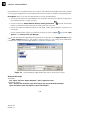


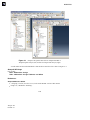


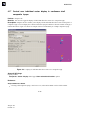


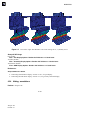


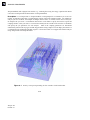


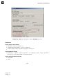


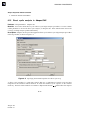


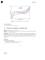


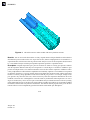


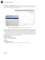


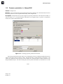


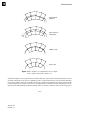


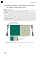
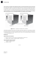

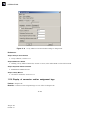
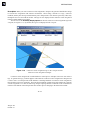

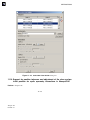


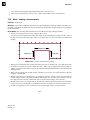


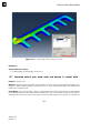

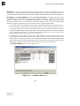


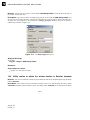


![[U2.05.02] Notice d`utilisation de la méthode X-FEM](http://vs1.manualzilla.com/store/data/006356186_1-353dbab293f9b25dc929c8fcb4e5fa0d-150x150.png)