Download ABSTRACT PAPROCKI, DANIEL. A Quantitative

ABSTRACT
PAPROCKI, DANIEL. A Quantitative Analysis to Determine Methods to Improve an
Industrial Compressed Air System. (Under the direction of Dr. Stephen Terry).
Compressed air systems are an integral part of many manufacturing facilities. Compressed
air is used for many things, including pneumatic controls, manufacturing equipment, air
motors, air tools, and blow off nozzles. Despite the versatility of compressed air, it comes at
a great cost, as approximately 80 percent of the energy used by the air compressor is rejected
as heat. The remaining 20 percent of the energy is converted to compressed air. Thus, it is
important to produce and use compressed air as efficiently as possible, which controls can
help accomplish.
The subject facility has a compressed air system that consists of four rotary screw type
compressors. Currently this system of compressors is not using system master controls,
which would help sequence the compressors according to compressed air demand.
After collecting amperage and pressure readings through data logging, several analyses were
carried out. First, a method to estimate power factor was created, then compressor power for
each compressor was calculated using amperage, power factor, and compressor motor
efficiency. Additionally, a technique to calculate volumetric flow using compressor power
was developed. The estimation of power factor and volumetric flow are essential when
determining compressor power and analyzing compressed air systems as a whole.
The free software package, AIRMaster+, made available by the Department of Energy,
allows the modeling of a compressed air system, and the simulation of energy efficiency
measures. Using this program, the subject facility’s compressed air system was modeled and
then energy efficiency measures were simulated. First, an automatic sequencer was simulated
to control the system air pressure to a reduced pressure of 95 psig, and to decide which
combination of compressors will adequately meet compressed air demand. The second
measure was to reduce the air leak load. The reduction of air leaks will reduce the
compressor capacity, which then reduces compressor power.
The measures result in cost savings of $52,377 per year, a 128 kW demand reduction, and
804,436 kWh per year in energy reduction. The total project cost is estimated to be $10,800,
giving a simple payback of approximately three months.
© Copyright 2013 by Daniel Paprocki
All Rights Reserved
A Quantitative Analysis to Determine Methods to Improve an Industrial Compressed Air
System
by
Daniel John Paprocki
A thesis submitted to the Graduate Faculty of
North Carolina State University
in partial fulfillment of the
requirements for the degree of
Master of Science
Mechanical Engineering
Raleigh, North Carolina
2014
APPROVED BY:
_______________________________
Dr. Stephen Terry
Committee Chair
________________________________
Dr. Alexei Saveliev
______________________________
Dr. Herbert M Eckerlin
ii
DEDICATION
I would like to dedicate this work to my parents Gerald and Cathi for showing me their
support during my extensive stay as a student at North Carolina State University.
iii
BIOGRAPHY
Daniel John Paprocki was born in the year of our lord 1988 in Durham, North Carolina,
shortly after Daniel’s parents relocated from Milwaukee, Wisconsin. At the age of two,
Daniel’s family made the decision to move 20 miles from Durham to the burgeoning
suburban community of Cary, North Carolina.
During Daniel’s elementary school years, he gained an interest in mathematics and sciences,
which only grew stronger as he got older. Daniel acquired an appreciation for hands on skills
during his formative years. Gerald, Daniel’s father would frequently have a home
improvement project to work on, and would inevitably recruit Daniel to help out.
Additionally, instead of taking the family cars to the shop, Gerald would routinely change the
oil and make simple repairs, and always would have Daniel pitch in to acquire these valuable
skills. This gave Daniel an appreciation for hard work, the satisfaction of saving money by
being self-reliant.
During Daniel’s senior year of High School, he applied to North Carolina State University in
Raleigh, North Carolina. In the fall of 2007, his first year at N.C. State, he decided to study
Engineering and German, and was able to matriculate into Mechanical Engineering after his
first year. Mechanical Engineering is a demanding discipline to succeed in, and with a second
major in German Studies, Daniel had his work cut out for him. With the double major,
graduating in the standard four years would be next to impossible. The German Studies
iv
major required a semester studying in Germany, which would take a whole semester and
summer away from engineering. Daniel spent the spring and summer of 2009 in Europe to
study in Germany. The semester abroad in Germany proved to be trying, but eye-opening.
Immersing in another culture and language is a rare and excellent way of expanding one’s
horizons, but can be exhausting. While in Germany, Daniel spent time with old friends, met
many new and interesting people, saw beautiful cities, artwork, and landscapes.
Once back at N.C. State, Daniel continued to march through his Engineering and German
courses. Of the topics within Mechanical Engineering, the thermal sciences interested Daniel
the most. During the fall of 2011, Daniel decided to apply for the State Energy Internship
Program, which was headed by Dr. Stephen Terry of the Mechanical Engineering
Department. This Internship offered Daniel his first hands on engineering experiences.
Daniel worked on several measurement and verification projects and was able to attend four
energy surveys through the Industrial Assessment Center at N.C. State. After the internship
ended, Dr. Terry offered Daniel a position within the IAC.
After graduating in December of 2012 with degrees in both Mechanical Engineering and
German Studies, Daniel applied to N.C. State’s Mechanical Engineering graduate program,
under the direction of Dr. Stephen Terry. Daniel’s concentration within Mechanical
Engineering is Thermal Sciences. Daniel has attended approximately 40 energy surveys as a
member of the IAC, and has been the lead graduate student on several reports.
v
Outside of school Daniel enjoys lifting weights, running, and going to the gym. Daniel also
enjoys collecting and listening to vinyl records. Additionally, Daniel loves spending time
with friends and family, playing card and board games, and playing fetch with Seamus.
vi
ACKNOWLEDGMENTS
I would like to thank and recognize several people that helped make this work possible. I
would first like to thank my parents, Gerald and Cathi Paprocki for their endless support and
patience during my pursuit to earn undergraduate degrees in Mechanical Engineering and
German Studies, and a Master’s degree in Mechanical Engineering. Undoubtedly, it required
a great deal of patience during this length of time. I would also like to thank my brother
Nathan, and sisters Katie and Jennifer for their show of support and love during this process.
I would like to thank all good friends including, but not limited to, Connor McDonald,
Patrick Murray, Sam Gates, Jackson Wooten, Kiran Thirumaran, and Taylor Atkins for their
encouragement throughout the process. Additionally, I would like to thank Laura for her
encouragement during the writing process.
I would like to state my utmost appreciation to the subject facility for access to their
compressed air system, their cooperation throughout the process, and assistance in collecting
all necessary data.
I would also like to thank Dr. Stephen Terry, whose support and guidance has not only made
this work possible, but has made a Master’s degree a realistic possibility for me. I will be
forever thankful for the many invaluable opportunities provided to me.
vii
I would also like to thank Dr. Herbert Eckerlin and Alexei Saveliev for serving on my
graduate committee advisory committee. I greatly appreciate your participation in this
project.
viii
TABLE OF CONTENTS
LIST OF TABLES ................................................................................................................... xi
LIST OF FIGURES ................................................................................................................ xii
Chapter 1 – Introduction ........................................................................................................... 1
1.1 Electrical Energy and Compressor Use in the United States .......................................... 2
1.2 Compressed Air Benefits and Drawbacks ...................................................................... 3
1.2.1 Inappropriate Compressed Air Use .......................................................................... 4
1.3 Introduction to Compressor Controls.............................................................................. 5
1.4 Main Project Objective ................................................................................................... 7
Chapter 2 –Compressed Air ...................................................................................................... 9
2.1 Important Compressed Air Terminology ........................................................................ 9
2.2 Types of Compressors................................................................................................... 12
2.3 Positive Displacement Compressors ............................................................................. 14
2.3.1 The Reciprocating Compressor.............................................................................. 14
2.3.2 Rotary Screw Compressors .................................................................................... 19
2.4 Dynamic Compressors .................................................................................................. 24
Chapter 3 – Compressor Controls ........................................................................................... 26
3.1 Basic Individual Compressor Controls ......................................................................... 26
3.1.1 Start/Stop Control .................................................................................................. 26
3.1.2 Load/Unload Control ............................................................................................. 27
3.1.3 Modulating Control ................................................................................................ 33
3.1.4 Dual/Auto and Variable Displacement .................................................................. 36
3.1.5 Variable Speed Drive Control ................................................................................ 37
3.2 Centrifugal Compressor Operation and Control ........................................................... 38
ix
3.3 Multiple Compressor Control ....................................................................................... 41
3.3.1 Cascade Control ..................................................................................................... 42
3.3.2 Network Controls ................................................................................................... 43
3.3.3 System Master Controls ......................................................................................... 45
3.3.4 Pressure/Flow Controllers ...................................................................................... 47
Chapter 4 – Data Collection .................................................................................................... 50
4.1 Measurement Equipment .............................................................................................. 51
4.2 Measurement Procedure and Data Collection............................................................... 56
4.3 Data Analysis ................................................................................................................ 58
4.3.1 – Power Factor Analysis ........................................................................................ 59
4.3.2 - 100 hp Air Compressor Data Analysis ................................................................ 64
4.3.3 – 150 hp Air Compressor Data Analysis ............................................................... 69
4.3.4 – 500 hp Air Compressor Data Analysis ............................................................... 72
4.3.5 – 600 hp Air Compressor Data Analysis ............................................................... 74
4.3.6 – Combined Analysis ............................................................................................. 76
4.3.7 – Volumetric Flow Analysis .................................................................................. 81
4.3.8 – Pressure Analysis ................................................................................................ 95
Chapter 5 - AIRMaster+ System Modeling .......................................................................... 100
5.1 Modeling the Compressed Air System ....................................................................... 100
5.1.1 Company Module................................................................................................. 102
5.1.2 Utility Module ...................................................................................................... 103
5.1.3 Facility Module .................................................................................................... 104
x
5.1.4 System Module .................................................................................................... 105
5.1.5 Compressor Module ............................................................................................. 107
5.1.6 LogTool................................................................................................................ 116
5.1.7 Profile Module ..................................................................................................... 124
5.2 Energy Efficiency Measures ....................................................................................... 130
5.2.1 Reduce System Air Pressure AIRMaster+ Validation ......................................... 131
5.2.2 Automatic Sequencer ........................................................................................... 137
5.2.3 Reduce Air Leaks ................................................................................................. 143
5.2.4 Total Savings ....................................................................................................... 147
Chapter 6 – Conclusions ....................................................................................................... 149
6.1 Data Analysis Conclusions ......................................................................................... 149
6.2 AIRMaster+ Conclusions ........................................................................................... 152
6.3 Further Opportunities .................................................................................................. 154
REFERENCES ..................................................................................................................... 155
APPENDICES ...................................................................................................................... 157
Appendix A-AIRMaster+ Automatic Sequencer Existing and Proposed Scenarios ........ 158
Appendix B-AIRMaster+ Automatic Sequencer Results ................................................. 162
Appendix C-AIRMaster+ Reduce Air Leaks Inputs ......................................................... 166
Appendix D-AIRMaster+ Savings Summary ................................................................... 167
xi
LIST OF TABLES
Table 1: Inappropriate Uses of Compressed Air and Alternative Methods (5) ........................ 5
Table 2: Facility Compressors ................................................................................................ 50
Table 3: Motor Efficiencies .................................................................................................... 59
Table 4: 100 hp Compressor Power Factor............................................................................. 61
Table 5: % Full Load Amperage and Power Factor ............................................................... 63
Table 6: System Profile Totals .............................................................................................. 129
Table 7: 600 hp System Pressure Reduction Results ............................................................ 133
Table 8: Savings from Reducing Compressor Pressure ........................................................ 134
Table 9: AIRMaster+ Baseline Operating Results ............................................................... 142
Table 10: AIRMaster+ Use Automatic Sequencer Results .................................................. 142
Table 11: AIRMaster+ Savings Resulting from Automatic Sequencer ................................ 143
Table 12: AIRMaster+ Reduce Air Leaks Results ............................................................... 147
Table 13: AIRMaster+Reduce Air Leaks Savings ............................................................... 147
Table 14: AIRMaster+ Savings Summary ............................................................................ 148
xii
LIST OF FIGURES
Figure 1: Percent of Energy Generation for Various Sources (1) ............................................. 2
Figure 2: Compressor Subsets (2) ........................................................................................... 13
Figure 3: Reciprocating Compressor Cross Section (9) ......................................................... 15
Figure 4: Piston at Top Dead Center....................................................................................... 16
Figure 5: Air Intake ................................................................................................................. 16
Figure 6: Piston at Bottom Dead Center ................................................................................. 17
Figure 7: Top Dead Center ..................................................................................................... 17
Figure 8: Compression Cycle.................................................................................................. 18
Figure 9: Double Acting Reciprocating Compressor (4) ........................................................ 19
Figure 10: Rotary Screw Compressor (3) ............................................................................... 20
Figure 11: Oil-flooded Screw Compressor (10) ..................................................................... 22
Figure 12: Oil-free (4) ............................................................................................................. 23
Figure 13: Impeller of Centrifugal Compressor (4) ................................................................ 25
Figure 14: Load/Unload Cycle................................................................................................ 29
Figure 15: Short Cycle ............................................................................................................ 31
Figure 16: Average kW vs Average Capacity with Load/Unload Capacity Controls (11) .... 32
Figure 17: Compressor Inlet Butterfly Valve 40% Open ....................................................... 34
Figure 18: Percent kW Input Power vs. Compressor Capacity for Modulation (11) ............. 35
Figure 19: Variable Displacement Control (8) ....................................................................... 37
Figure 20: VSD Curve (8)....................................................................................................... 38
xiii
Figure 21: Centrifugal Compressor Performance Curve (12)................................................. 39
Figure 22: The Effect of Inlet Air Temperature (11) .............................................................. 41
Figure 23: Compressors in Cascade (11) ................................................................................ 42
Figure 24: Network Controls .................................................................................................. 45
Figure 25: Pressure Flow Controller with One Compressor Room (11) ................................ 48
Figure 26: FlexSmart TRMS Module ..................................................................................... 51
Figure 27: HOBO Energy Logger........................................................................................... 52
Figure 28: 200 AMP Current Transducer ............................................................................... 53
Figure 29: Data Logger Setup ................................................................................................. 53
Figure 30: Launching a Device ............................................................................................... 54
Figure 31: Launch Logger Interface ....................................................................................... 55
Figure 32: Configure Sensor ................................................................................................... 56
Figure 33: AIRMaster+ Power Calculator .............................................................................. 60
Figure 34: Power Factor vs. Amperage .................................................................................. 62
Figure 35: Power Factor vs. Percent Full Load Amperage ..................................................... 64
Figure 36: 100 hp Compressor Amps from Raw Data ........................................................... 65
Figure 37: 100 hp Compressor Power from Averaged Data Points........................................ 67
Figure 38: 100 hp Compressor Load/Unload Cycle ............................................................... 68
Figure 39: 150 hp Compressor Amperage .............................................................................. 69
Figure 40: 150 hp Compressor Power .................................................................................... 71
Figure 41: Illustration of Modulation ..................................................................................... 72
xiv
Figure 42: 500 hp Compressor Amperage .............................................................................. 73
Figure 43: 500 hp Compressor Power .................................................................................... 74
Figure 44: 600 hp Compressor Amps ..................................................................................... 75
Figure 45: 600 hp Compressor Power .................................................................................... 76
Figure 46: Plot of Compressor Power and Pressure ............................................................... 78
Figure 47: System Compressor Power and System Pressure.................................................. 80
Figure 48: Compressed Air Demand (CFM) .......................................................................... 82
Figure 49: System Compressor Power February 21 to February 27 ....................................... 83
Figure 50: Compressed Air Demand and Compressor Power ................................................ 84
Figure 51: CFM vs. hp with Linear Regression ...................................................................... 86
Figure 52: Actual CFM and Predicted CFM........................................................................... 89
Figure 53: Estimated Volumetric Flow................................................................................... 91
Figure 54: Estimated Volumetric Flow Excluding Outliers ................................................... 93
Figure 55: Estimated Volumetric Flow and System Pressure ................................................ 94
Figure 56: System Pressure Varying with Compressor Power ............................................... 95
Figure 57: Pressure vs. Power (60 hp-120 hp) ........................................................................ 96
Figure 58: System Pressure vs. Compressor Power (210 hp to 270 hp) ................................. 98
Figure 59: Pressure vs. Compressor Power (500 hp to 800 hp).............................................. 99
Figure 60: AIRMaster+ Home Screen (15) .......................................................................... 101
Figure 61: AIRMaster+ Company Screen (15) ..................................................................... 102
Figure 62: AIRMaster+ Utility ............................................................................................. 103
xv
Figure 63: AIRMaster+ Facility Information (15) ................................................................ 104
Figure 64: AIRMaster+ Facility Compressor Summary (15) ............................................... 105
Figure 65: AIRMaster+ System Module (15) ....................................................................... 106
Figure 66: AIRMaster+ System Module Daytypes (15) ....................................................... 107
Figure 67: AIRMaster+ Compressor Module (15) ............................................................... 108
Figure 68: AIRMaster+ Compressor Module Compressor Catalog (15).............................. 109
Figure 69: AIRMaster+ Compressor Catalog Search (15) ................................................... 110
Figure 70: Compressor Inventory (15) ................................................................................. 111
Figure 71: 100 hp Compressor Performance Profile (15) ..................................................... 112
Figure 72: 150 hp Compressor Performance Profile (15) ..................................................... 113
Figure 73: 500 hp Compressor Performance Profile (15) ..................................................... 114
Figure 74: 600 hp Compressor Performance Profile (15) ..................................................... 114
Figure 75: Log Tool Opening Screen (16) ............................................................................ 117
Figure 76: LogTool Imported Loggers (16).......................................................................... 118
Figure 77: 100 hp Compressor Daytypes (16) ...................................................................... 119
Figure 78: Plot of 100 hp Compressor Daytypes .................................................................. 120
Figure 79: LogTool 150 hp Compressor Daytypes (16) ....................................................... 121
Figure 80: Plot of 150 hp Compressor Daytypes .................................................................. 121
Figure 81: 500 hp LogTool Daytypes Plot (16) .................................................................... 122
Figure 82: 600 hp Compressor LogTool Daytypes (16) ....................................................... 123
Figure 83: 600 hp Compressor Daytypes.............................................................................. 123
xvi
Figure 84: System Profile Module Production Daytype (15) ............................................... 124
Figure 85: Production Profile Compressor Volumetric Flow (15) ....................................... 125
Figure 86: Figure 85: Production Profile Compressor Power (15) ....................................... 126
Figure 87: Saturday Profile Volumetric Flow (15) ............................................................... 127
Figure 88: Saturday Profile Data Power (15) ....................................................................... 127
Figure 89: Sunday Profile Volumetric Flow (15) ................................................................. 128
Figure 90: Sunday Profile Power (15) .................................................................................. 129
Figure 91: 600 hp Compressor Production Profile (15) ....................................................... 131
Figure 92: Sample Pressure Reduction Simulation (15) ....................................................... 133
Figure 93: Energy Efficiency Measures (15) ........................................................................ 138
Figure 94: AIRMaster+ Use Automatic Sequencer Measure (15)........................................ 140
Figure 95: AIRMaster+ Automatic Sequencer Hourly Data (15) ......................................... 141
Figure 96: AIRMaster+ Reduce Air Leaks ........................................................................... 146
1
Chapter 1 – Introduction
Industrial manufacturing, a vital component to the United States economy, requires a
significant amount of energy during production. The energy consumed by industry is
distributed to a diverse number of end users, which may include ovens, electric boilers,
robotics, manufacturing machinery, HVAC, lighting, and, lastly, air compressors. Utilities
must provide the energy to manufacturing facilities to run all of these systems, but this comes
at a large cost. The substantial energy consumption comes at a price, which cuts directly into
profit margins. Compressed air, which is often a necessity to manufacturers, comprises a
significant segment of energy consumption in the average manufacturing facility. For the
reason that energy costs can directly influence profits and compressed air encompasses a
large percentage of the energy use in a manufacturing facility, finding any means to increase
efficiency of compressed air systems should be a high priority. This project will analyze an
actual compressed air system, and attempt to identify methods to increase the overall
efficiency, with a focus on compressor controls, and how to operate a system of compressors
efficiently and to meet compressed air demand.
2
1.1 Electrical Energy and Compressor Use in the United States
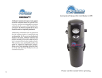
The United States relies on several sources of energy for the production of electricity. This
includes coal, natural gas, nuclear, hydro, oil, and finally renewables. The percent of
generation for each energy source, for 2011, is shown in Figure 1 below (1)
Figure 1: Percent of Energy Generation for Various Sources (1)
As shown above, coal represents the largest percentage of electricity generation, followed by
natural gas and nuclear. In 2011, the total U.S. electrical energy consumption was 3,882
billion kWh (1). In addition to electricity, natural gas is also commonly used in
manufacturing facilities.
3
U.S. Manufacturers consume nearly 26% of all electrical energy consumed in the United
States (2). Approximately 10% of electricity consumed in manufacturing facilities is from
compressed air. Thus, 2.6% of all energy consumed in the United States is consumed by air
compressors in an industrial setting (3). This represents a staggering 101 billion kWh per
year. To put this into perspective, 101 billion kWh could power the average American home,
using 1,200 kWh per month, for over 84 million years. At an average energy price of
$0.062/kWh, the total electrical cost to run industrial air compressors is $2.6 billion per year
(1). Considering the high energy consumption and energy cost of operating compressed air
systems, it would behoove manufacturers to attempt to increase the efficiency of their
systems, to capture significant savings.
1.2 Compressed Air Benefits and Drawbacks
It is important to understand why we use compressed air. Compressed air is a fundamental
utility at many industrial sites and manufacturing facilities, just as important as power and
fuel. Compressed air can have many important uses, including operating pneumatic tools,
motors, pneumatic cylinders, automation equipment, conveyors, and controls schemes. There
are also many specific compressed air uses in manufacturing processes, including oxidation,
fractionation, cryogenics, refrigeration, filtration, dehydration, and aeration (4). A facility
may also use compressed air for an application, as opposed to electricity, in a combustible
environment, such as a chemical plant. Although compressed air has many appropriate uses,
inappropriate uses, in which a more efficient method could be used, can have high costs.
4
Despite the effectiveness and flexibility of compressed air, unfortunately the overall
efficiency of a typical compressed air system is only 10% to 15%. This is due to losses from
the heat of compression, meaning that approximately 80% of the electrical energy consumed
by air compressors is converted to heat and not compressed air. Thus, the use of electricity
instead of compressed air is much more efficient. To illustrate this issue, we will compare the
operating cost of a one hp compressed air motor to a standard one hp electric motor. A
typical one hp compressed air motor requires 30 scfm at 90 psig, which requires
approximately 7 hp at the compressor shaft. Therefore, the compressed air motor will require
7 times as much electrical input, and money, to produce the same amount of work as a
standard one hp motor. This indicates that one should be judicious when determining whether
or not compressed air should be used for a certain task at a manufacturing facility.
1.2.1 Inappropriate Compressed Air Use
Considering the expensive and inefficient nature of compressed air as a utility, inappropriate
compressed air uses must be kept to a minimum. An inappropriate compressed air use is
defined as any application that can be done more efficiently by a method other than
compressed air (5). Provided below is a table from the Industrial Technologies Program,
which lists potentially inappropriate uses and a suggested alternative to that use.
5
Table 1: Inappropriate Uses of Compressed Air and Alternative Methods (5)
Potentially Inappropriate Uses
Clean-up, Drying, Process
Cooling
Sparging
Aspirating, Atomizing
Padding
Vacuum generator
Personnel cooling
Open-tube, compressed airoperated vortex coolers without
thermostats
Air motor-driven mixer
Air-operated diaphragm pumps
Idle equipment
Abandoned equipment
Suggested Alternatives/Actions
Low-pressure blowers, electric fans, brooms,
nozzles
Low-pressure blowers and mixers
Low-pressure blowers
Low to medium -pressure blowers
Dedicated vacuum pump or central vacuum
system
Electric fans
Air-to air heat exchanger or air conditioner, add
thermostats to vortex cooler
Electric motor-driven mixer
Proper regulator and speed control; electric pump
Put an air-stop valve at the compressed air inlet
Disconnect air supply to equipment
1.3 Introduction to Compressor Controls
Compressor controls can vary from compressor to compressor, and can be unique to a
compressor system based on the number and types of compressors the system is comprised
of. As the number of compressors in a system increases, so does the complexity of the
required controls.
Single air compressor systems can consist of two distinct compressor types, those being
positive displacement and dynamic compressors. Typically, positive displacement machines
are controlled by on/off, load/unload, modulation, or VFD control types.
6
On/off controls are generally found in smaller reciprocating compressors. When the desired
system pressure is reached, the reciprocating compressor simply shuts down. The compressor
will subsequently turn back on when the system pressure reaches a set minimum allowable
pressure. For larger rotary screw compressors, load/unload and modulation are commonly
employed. Using load/unload controls will track system demand and help save energy while
unloaded. This will also ensure that the compressor does not turn on and off in short cycles,
which can destroy larger motors from locked-rotor current. Load/unload controls allow the
compressor to unload when the system pressure reaches a predetermined maximum.
Modulation controls are typically found in rotary screw and dynamic compressors.
Modulation follows system demand by restricting the flow of air to the compressor through
the use of an inlet valve, such as a butterfly valve. As less air flows through the inlet, less
power is required to compress that air. However, the main drawback of using modulation is
that it reduces the pressure of the inlet air, causing the compression ratio to increase. For
flooded oil rotary screw compressors utilizing modulation, the percent kW input at 50
percent capacity will likely be approximately 85%, which is rather inefficient. Allowing less
air through the inlet increases the compressor efficiency, but the decreased pressure at the
inlet is akin to taking a step backward.
Variable frequency drives are generally found in rotary screw compressors. The variable
frequency drives allow the motor to track system demand by altering the speed of the electric
7
motor by varying voltage frequency. The motor speed and percent power have approximately
a one to one ratio, meaning that at half the fully rated revolutions per minute the motor will
draw half the fully rated power input. Compressor capacity and motor speed also have a one
to one ratio, which implies that at half capacity the compressor will only require half of its
fully rated power. This is a rather efficient method of controlling a single compressor.
As compressor systems grow larger, it is important for compressors to communicate with
each other, helping to ensure compressors only turn on when necessary. Generally network
controls are utilized to make certain compressors communicate with each other. More
complicated systems, such as those with multiple compressor rooms consisting of both
centrifugal and positive displacement compressors, require System master controls. System
master controls allow for the control of large compressed air systems through measurement
of system parameters; pressure for instance. Further description of each of the
aforementioned control methods is detailed in Chapter 3.
1.4 Main Project Objective
The main objective of this study is to collect data from a subject facility’s compressed air
system using data loggers, analyze data, and then to model the compressed air system using
AIRMaster+, which is a free software package made available by the Department of Energy.
After the compressed air system is modeled in AIRMaster+, the software will simulate
various energy efficiency measures, one of which is using an automatic sequencer. An
8
automatic sequencer is essentially system master controls, which help operate lager
compressed air systems efficiently. To understand how multiple compressors operate
together, first a familiarity of different types of compressors and an understanding of various
methods of single compressor and multiple compressor controls must be realized.
Through the simulation of the implementation of an automatic sequencer using AIRMaster+,
the potential energy and cost savings associated with sophisticated compressed air system
controls can be conveyed to the subject facility.
9
Chapter 2 –Compressed Air
Modern manufacturing facilities utilize multiple types of air compressors to meet the
compressed air demand for their processes. Currently, the most common compressors used in
the industrial world are reciprocating compressors, rotary screw compressors, and lastly,
centrifugal compressors. Based on the application and compressed air demand of the
manufacturing facility, a type of compressor is chosen. Each compressor has its own benefits
and drawbacks, which must be considered before purchase and installation. This chapter will
discuss compressed air terminology, common compressed air components, and types of
compressors.
2.1 Important Compressed Air Terminology
In order to gain a better understanding of compressed air systems, it is important to become
familiar with terminology related to compressed air.
Capacity: Capacity is the amount of air delivered under specific conditions. This is usually
measured in cubic feet per minute, or CFM (6).
Cubic Feet Per Minute (CFM): This is the volumetric flow rate (6).
Actual CFM (ACFM): Flow rate of air at a certain point at the actual temperature
and pressure at that point. When this is used for the capacity of an air compressor, it
is measured at prevailing ambient conditions of temperature, pressure, and relative
humidity (6).
10
Inlet CFM (ICFM): The volumetric air flow rate through the compressor inlet valve
under the prevailing ambient conditions. For positive displacement machines ICFM
and ACFM should be identical, but could be different in some centrifugal air
compressor designs due to air losses through shaft seals (6).
Standard CFM (SCFM): The volumetric flow of free air measured and converted to
a standard set of reference conditions. The International Standards Organization
(ISO) defines standard air as 14.5 psia, 68°F, and 0%relative humidity (6). This is
equivalent to specifying mass flow rate, since a volume at a given temperature and
pressure has a specific density.
Demand: The CFM of air required by a specific point in a facility, or by the entire facility.
This is generally referenced to scfm.
Humidity, Relative: Relative humidity is the ratio of the actual vapor pressure to the vapor
pressure if the air were completely saturated (7).
Dew Point: The dew point is the temperature at which water vapor will begin to
condense out of air if the air is cooled at constant pressure.
Specific Humidity: The mass of water vapor in an air vapor mixture per mass of dry
air.
Power: Power is work over a period of time. Power is often measured in measured in kW, or
brake horsepower.
Brake Horsepower (bhp): This is the horsepower required at the compressor shaft to
produce compressed air.
11
Load Factor: Load factor is the average compressor load divided by the maximum
rated compressor load over a period of time.
Full-Load: When the air compressor is operating at full speed with a fully open inlet
and delivering maximum air flow.
Specific Power: A method of measuring compressor operating efficiency, usually in
the form bhp/100 ACFM, or kW/100 ACFM.
Total package Input Power: This is the total power used by the air compressor,
including the drive motor, fans, motors, and controls.
Pressure: Pressure is defined as force per unit area. This is commonly measured in pounds
per square inch (psi).
Atmospheric Pressure: This is the naturally occurring pressure in the atmosphere.
The atmospheric pressure at sea level is approximately 14.7 psi.
Gauge Pressure: Pressure determined by instruments, which are calibrated so that
atmospheric pressure is zero psi. Gauge pressure is expressed as psig.
Pressure Drop: Pressure drops occur in compressed air systems due to friction or
restrictions.
Pressure Range: The range between minimum and maximum pressures for an air
compressor. Also referred to as load-no load pressure ranges.
Rated Pressure: The ideal pressure for optimal compressor performance.
Receiver: A pressure vessel used to store compressed gas or air.
12
Surge: A dangerous and destructive operating condition for centrifugal air compressors. This
occurs when a reduced flow rate results in backwards flow. The compressor can no longer
overcome backpressure.
2.2 Types of Compressors
Industrial compressors are divided into two main types of compressors, which are positive
displacement and dynamic. For the positive displacement compressor, a finite quantity of air
or gas enters into a compression chamber and the volume of the chamber is mechanically
reduced, thereby increasing the pressure of that gas before discharge (4). Dynamic
compressors, such as centrifugal compressors and axial flow compressors, operate much
differently. By means of impellers rotating at an extraordinary speed, a dynamic compressor
imparts kinetic energy to continuously flowing air. The kinetic energy of the air or gas is
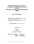
changed into potential energy (pressure) by the impellers and diffusers (4). Below is a figure
that further breaks air compressors into subcategories.
13
Figure 2: Compressor Subsets (2)
14
2.3 Positive Displacement Compressors
Positive displacement compressors are available in two distinct categories, which are
reciprocating and rotary screw compressors. Reciprocating compressors are divided further
into single-acting and double-acting, both of which operate similar to that of a bicycle pump
to compress air. Industrial facilities also commonly use rotary screw compressors, which
compress air by trapping air inside the rotors and compress the air as it travels down rotors to
the discharge point (4). Rotary screw compressors are often oil flooded to lubricate the
rotors, but oil free is also available.
2.3.1 The Reciprocating Compressor
Typically, the modern reciprocating compressor used in manufacturing facilities are between
5 hp and 30 hp. Single acting reciprocating compressors are generally available up to 150 hp
and can produce higher than 175 psig compressed air. (8) For a single acting reciprocating
air compressor, the operating efficiency is between 22 and 24 kw/100 CFM. In general, a
double acting reciprocating compressor can achieve an operating efficiency of 15 to 16
kW/100 CFM.
Reciprocating compressors are often staged to improve efficiency, with an intercooler
between stages. Most reciprocation compressor systems have two stages to produce 100 psig
15
air. Three or more stages may be used where high pressure (greater than 150 psig) is needed,
such as in blow molding operations.
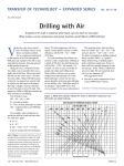
Figure 3 below is a cross section of a reciprocating compressor with three pistons to produce
compressed air.
Figure 3: Reciprocating Compressor Cross Section (9)
The single acting reciprocating compressor is distinguished by a piston and cylinder, similar
to that of an internal combustion engine, which is driven by a connecting rod from the crank
(4). The reciprocating compressor is essentially a piston cylinder device with an inlet and exit
valve. The compression cycle starts when the piston is at top dead center, when the piston
volume is zero, not including the clearance volume.
16
Figure 4: Piston at Top Dead Center
As the crank shaft turns, the piston moves down in the cylinder, thereby increasing the piston
volume and creating a vacuum. The intake valve allows atmospheric air to enter the chamber
during this process (3).
Figure 5: Air Intake
At the intake valve, atmospheric pressure is higher than the pressure in the cylinder, therefore
air enters the cylinder. At bottom dead center, the intake valve is closed, and the piston is
driven back up the cylinder by the crank shaft (3).
17
Figure 6: Piston at Bottom Dead Center
The volume in the cylinder decreases as the piston moves towards top dead center, which
increases the pressure. At the desired gauge pressure, the exhaust valve opens and the
compressed air is released from the cylinder. The desired compressor pressure is often
controlled by a spring, which will force the exhaust valve shut. The spring may be adjusted to
allow for different pressure settings (3).
Figure 7: Top Dead Center
18
At the end of the cycle the compressed air is released, and both the intake and exhaust valves
are closed. The cycle repeats until the demand for compressed air is satisfied, at which point
the compressor will shut off. Commonly the power to drive this cycle is derived from an
electric motor. Figure 8 below details the complete compression cycle (3).
Figure 8: Compression Cycle
The double acting reciprocating compressor is similar to the single acting reciprocating
compressor, but with one exception. Double acting means that the compressor uses both
sides of the piston and cylinder for air compression, effectively doubling the capacity for a
giving cylinder size. This type of compression is particularly efficient with multi-stage
compressors (4).
19
Figure 9: Double Acting Reciprocating Compressor (4)
Using a reciprocating compressor to produce compressed air can have advantages. Generally,
reciprocating air compressors are small in size and weight, and therefore can be located close
to the point of use. This would avoid long lengths of compressed air piping and potential
pressure drops. Also, reciprocating compressors generally require simple maintenance
procedures. Unfortunately, reciprocating compressors are associated with a high initial cost,
and high vibrations, which require a thick foundation (4).
2.3.2 Rotary Screw Compressors
Oil flooded rotary screw compressors and oil-free rotary screw compressors are two common
types of rotary screw compressors. The more common air compressors found in industry
20
today is the oil flooded rotary screw compressor, due in part to its versatility (4). The
operation of the screw compressor is distinctly different than the aforementioned
reciprocating compressor. The rotary screw compressor mechanically compresses air with
two screws, one of which, the male screw, is driving the female screw. These screws are
meshed together in a stator and rotate. Air flows through the inlet port and becomes trapped
between the meshing screws. As the screws rotate, the point of intermeshing, where the air is
trapped, moves gradually along the axial length of the rotors. As this occurs the space
occupied by air reduces in volume, resulting in an increase in pressure. Air compression
follows until the air reaches the discharge port and the air is released to the demand side of
the compressed air system (4). Figure 10 depicts the two screws meshed together.
Figure 10: Rotary Screw Compressor (3)
21
Lubrication is vital to health and longevity of the oil-flooded rotary screw compressor. The
lubrication serves three basic functions. The oil lubricates the meshing rotors and bearings,
and serves to intercool the air during compression. The lubrication also performs much like
oil in an automobile piston and cylinder system would, in that it acts as a clearance between
the meshing rotors. Thus, the rotors never touch, greatly reducing friction and heat (4).
Commonly, oil flooded rotary screw compressors are available from 3 hp to 900 hp, with
discharge pressures from 50 psig to 250 psig (4). Figure 11 is a schematic of a generic oilflooded screw compressor package.
22
Figure 11: Oil-flooded Screw Compressor (10)
Advantages of oil-flooded rotary screw compressors include relatively compact sizes for high
horsepower systems, low vibration, and accurate part load capacity control systems.
Disadvantages of an oil-flooded rotary screw compressor include the fact that lubricant can
carry over into the compressed air flow, and the system efficiency can vary depending on the
chosen control mode. One can expect to achieve operating efficiencies of 17 to 22 kW/100
CFM for single stage compressors, and 16 to 19 kW/100 CFM for two stage compressors (4).
23
The lubricant-free rotary screw compressor works in the same fashion as the oil-flooded
screw compressors. As the name would suggest, there is no lubrication injected in the
compression chamber. Additionally, there are two distinct types of oil-free rotary screw
compressors; dry type and water injected type. Figure 12 illustrates an oil-free rotary screw
system, with the distinct lubricated timing gears.
Figure 12: Oil-free (4)
A dry type oil-free screw compressor uses lubricated timing gears, which are external to the
compression chamber, to keep the intermeshing rotors from touching. These types of
compressors do not have coolant injected into the compression chamber, and therefore may
require two stages of compression, with an intercooler between stages and an after cooler
24
after the second stage, to compress air to higher pressures. This is similar to a reciprocating
compressor. Teflon may be used to help seal the rotors and limit friction between moving
parts. A one stage dry type compressor can operate up to 50 psig, whereas a two stage may
operate up to 150 psig.
Similarly, the water type lubricant-free rotary screw compressor uses timing gears. However,
in this type of compressor water is injected into the compression chamber. This acts to
remove the heat of compression and seal any internal clearances. An oil-free screw
compressor can be expected to operate at an efficiency of 18 to 22 kW/100 CFM. Although
these types of compressors produce oil-free compressed air, they have a higher initial cost,
are generally less efficient and require higher maintenance costs than their oil-flooded
counterparts (4).
2.4 Dynamic Compressors
The most common and widely used compressor used for large industrial applications is the
centrifugal compressor. Centrifugal compressors operate by converting the high velocity of
air flowing through an impeller to pressure energy. The impeller accelerates the continuously
flowing air stream to a high velocity, and then the compressor converts the kinetic energy to
pressure energy as the speed is reduced by means of a diffuser (4). Interestingly, as the
system pressure decreases, the compressor capacity to produce compressed air increases (4).
A centrifugal compressor will operate at an efficiency of 16-20 kW/100 CFM. (4) Also, it
25
should be noted that a centrifugal compressor will produce oil-free compressed air. Figure 13
depicts an impeller accelerating the flow of air through a compressor.
Figure 13: Impeller of Centrifugal Compressor (4)
26
Chapter 3 – Compressor Controls
The purpose of compressor controls is to match the compressor output with the facility
compressed air demand. This is done by sustaining the compressor discharge pressure
between a specified range. Developing a control strategy, whether for one compressor or
multiple air compressor systems, is vital to saving energy and money. First, controls for
individual compressors will be discussed, followed by multiple compressor system controls.
3.1 Basic Individual Compressor Controls
For smaller single compressor compressed air systems, controls are contained to the
compressor itself. Individual compressor types to be discussed are start/stop, load/unload,
modulating, dual/auto, variable displacement, and variable frequency drive control.
3.1.1 Start/Stop Control
For reciprocating compressors and rotary screw compressors under 25 hp, a simple Start/Stop
control scheme would be a satisfactory control method. The compressor motor turns off as a
specified pressure set point is reached and then turns back on when the pressure drops below
a given lower pressure set point.
27
A simple example of start/stop control is a home thermostat. During the winter, as the
temperature in a space dips below a set point temperature, the heating system will turn on to
supply heat. The temperature in the space will rise until it reaches another set point, at which
point the heating system will shut off. In this manner an average temperature is maintained.
The difference between the cut on point and cut off point is the deadband. The system will
operate between the two setpoints in this deadband region.
Depending on storage capacity, the pressure range, or deadband, needed for this control
method can be as high as 35 psi. This is a fairly simple control scheme, needing only a
pressure switch. Furthermore, this method can save energy, as the motor and compressor
operate only when required. However, the frequent full load amp starting can wear down a
motor, and can only be used with smaller motors.
3.1.2 Load/Unload Control
Load/Unload controls are a common control scheme for oil flooded rotary screw
compressors, but can be used for larger reciprocating and centrifugal compressors. As the
predetermined pressure set point is reached, the compressor is allowed to unload, which uses
a lower power setting and saves energy. To unload means to close the inlet air damper,
ceasing the production of compressed air, and slowly depressurizing the compressor. During
this process, the compressor is still pushing against the pressure in the sump, which requires
power, but the sump pressure is allowed to slowly decrease. Once the sump reaches about 15
28
psig, the compressor operates at fully unloaded conditions and draws 30% to 40% of its full
load power.
Decreasing the oil pressure too quickly would be analogous to shaking up an unopened soda
bottle. Shaking the soda bottle causes dissolved carbon dioxide in the liquid to be released
thus, increasing the pressure. If opened too quickly, the soda will foam and result in a mess.
The same phenomenon will occur in an oil flooded rotary screw compressor. Oil is
compressed along with air, and gas is dissolved in the lubricant. If the pressure is reduced too
quickly, the oil will foam and lose its ability to lubricate the rotors. For this reason the
compressor is blown down slowly. Figure 14 depicts the load/unload cycle of a real 100 hp
compressor.
In Figure 14 below, the compressor is fully loaded until approximately 13:38:10, at which
point the compressor unloads because the maximum system pressure set point is reached.
From 13:38:10 to 13:39:40 the compressor blows down and gradually uses less power. At
approximately 13:39:40 the compressor reloads when the system pressure falls to the
minimum pressure set point. At this point, the compressor demand rapidly increases until it
has reached full load. The compressor remains fully loaded until the desired system pressure
has been reached.
29
Figure 14: Load/Unload Cycle
30
Thus, some period of time is required to fully unload a rotary screw compressor. As the
pressure in the system drops to a fixed lower pressure, the compressor reloads. This method
of controlling higher powered compressors is advantageous compared to start/stop controls
because there is less stress on the electric motor, increasing the longevity of the compressor
package. However, if the compressed air system does not have enough storage, short cycles
may occur. Short cycles may cause premature wearing and energy savings may be reduced.
Compressed air storage is key to running an efficient load/unload control scheme. The
compressor will be more efficient with increased storage. For example, if a compressed air
system has one gallon/CFM of storage and is operating at 50% capacity, the compressor will
still be using approximately 84% of its kW input on average. This operating condition, the
result of low air storage, arises because the compressed air is depleted at a quick rate and the
compressor will need to load before the sump fully depressurizes and it is fully unloaded.
The compressor will begin to unload and decrease compressor power. However, before the
compressor can completely unload at 30% to 40% of its power, the compressor will reload
due to the fast depletion of compressed air in the system. Consequently, the compressor will
operate at a higher average percentage of its full load power during operation.
31
Figure 15: Short Cycle
Conversely, should a rotary screw compressor, using load/unload controls, have 5
gallons/CFM, the compressor would be consuming approximately 68% of its kW input. With
more storage, the compressed air in the system will deplete at a slower rate and the
compressor will have more time to remain unloaded, and therefore will use less energy.
Storage should be sized to ensure additional compressors will not need to be turned on in a
large demand event. Figure 16 plots the efficiency of running a load/unload control scheme
for a rotary screw compressor at 1 gallon of storage per CFM to 10 gallons of storage/CFM
(4) (11).
32
Figure 16: Average kW vs Average Capacity with Load/Unload Capacity Controls (11)
33
3.1.3 Modulating Control
Modulating controls are often used in industry for rotary screw and centrifugal compressors.
Modulation restricts the air flow through the inlet valve of the compressor to reduce the
production of compressed air. This allows for tighter pressure control and continuous motor
operation, reducing wear. Modulating also allows for accurate matching of capacity
production to compressed air demand. The main issue with modulation is that the pressure
ratios increase as the inlet valve is restricted, causing inefficient operation. As the inlet valve
closes the pressure at the inlet decreases accordingly. For example, a compressor using
modulating controls with an inlet valve 40 percent open will experience an inlet air pressure
of 40 percent of standard atmospheric pressure. Atmospheric pressure at sea level is
approximately 14.7 psia, therefore the inlet air pressure for the aforementioned operating
condition will be 5.88 psia. If the compressor is producing compressed air at 100 psig, the
new compression ratio is 17.5:1 as opposed to 7.8:1 (11). This is illustrated in Figure 17.
34
Figure 17: Compressor Inlet Butterfly Valve 40% Open
The result is that a modulating rotary screw compressor will require approximately 88% of
the total kW input to produce 50% of its capacity (4) (11). The energy savings come from the
reduced mass of the air being compressed. The following curve in Figure 18 illustrates the
relationship between percent kW input power and percent capacity for a rotary screw
compressor utilizing modulating controls.
35
Figure 18: Percent kW Input Power vs. Compressor Capacity for Modulation (11)
Modulating controls might be appropriate if a rotary screw compressor is operating with little
to no storage at higher capacity. Generally, rotary screw compressors can be switched to run
on either load/unload or modulating controls. Some compressors may allow modulation with
blowdown, which is a control method that allows the compressor to unload at some low
capacity. From Figure 18 above, a compressor using inlet modulation with blowdown would
use modulating control until about 40 percent capacity, at which point the compressor begins
using load/unload control.
36
3.1.4 Dual/Auto and Variable Displacement
The next control type is the Dual/Auto, which is for either small reciprocating compressors
or rotary screw compressors. For reciprocating compressors, dual/auto dual allows the
compressor to select either start/stop or load/unload. Dual/Auto Dual controls allow oilflooded rotary screw compressors to select between modulating and load/unload controls.
Furthermore, if unloaded for a long duration, this control type will shut down rotary screw
compressors.
Another control type available for rotary screw compressors is variable displacement.
Variable displacement effectively shortens the length of the screws by using a turn-valve,
spiral-valve, or a poppet-valve. This allows a decrease in the amount of air flowing through
the inlet, and in turn decreases the amount of power needed to compress air. This is an
effective way to increase and decrease compressor capacity. Variable displacement is
generally more efficient at running partially loaded compressors than even load/unload
controls with high storage. Figure 19, below, illustrates the relationship between percent kW
input power and percent capacity for a rotary screw compressor with variable displacement
control (4) (11).
37
Figure 19: Variable Displacement Control (8)
3.1.5 Variable Speed Drive Control
The most effective control method for operating at partial loads is using a variable speed
drive (VSD). The variable frequency drive adjusts the compressor capacity by changing the
speed of the electric motor as compressed air demand in the system changes. The compressor
capacity is proportional to the speed of the male rotor, but due to the design of variable
displacement drive package, at full load capacities the male rotor is rotating above the
optimum rotor speed. Thus, a compressor with a VSD will require more power at full load
than otherwise, but a VSD offers significant power reduction and energy savings at lower
loads. Figure 20 illustrates the relationship between percent kW input power and percent
capacity for an oil-flooded screw compressor with a variable speed drive (11).
38
Figure 20: VSD Curve (8)
3.2 Centrifugal Compressor Operation and Control
The operation characteristics of centrifugal air compressors are complex and affected by inlet
air density and intercooler cooling water temperature. The basic compressor performance
curve, pressure against flow, is determined by the design of the impeller. An example of this
is that an impeller with radial blades will yield a low rise in pressure as flow is decreased,
and backward leaning blades will create a higher rise in pressure as flow is decreased.
When operating centrifugal compressors it is important to control for surge and choke. Surge,
which is harmful to the machine, occurs when flow reverses in the diffuser after the air
leaves the impeller. This is possible because of an increased flow path length in the diffuser,
39
causing the flow to dissipate due to friction and ultimately the flow reverses (11). The
aerodynamic instability within the system is to the extent that the compressor can no longer
deliver the necessary pressure to produce flow downstream (12). To avoid the destructive
surge condition, centrifugal compressors may use discharge bypass or blow-off control. To
avoid surge, enough compressed air is discharged to atmosphere to keep the unit at some
minimum load, while the required capacity is delivered to the facility. For example, if the
facility needs only 45% capacity, the compressor will produce approximately 70% of its
capacity and blow-off the extra 25% of the compressed air. For this reason, blow-off is quite
wasteful and expensive, and therefore should be avoided. Figure 21 depicts the surge line in a
centrifugal compressor performance curve.
Figure 21: Centrifugal Compressor Performance Curve (12)
40
The opposite of surge is choke, or stonewall. This occurs at flow rates that are above the
design rate, which should not occur until the velocity at the impeller inlet reaches the speed
of sound. As the compressor exceeds the capacity limit, the performance enters the choke
area. At this point, any increase in flow rapidly decreases the pressure being produced (11).
Centrifugal compressors are designed to operate at pre-determined tip speed, which is usually
between Mach 0.85 and Mach 0.9. Thus, to increase and decrease the flow rate, an inlet
throttle valve is utilized. Additionally, the throttle valve reduces the pressure, and air density
at the inlet before the impeller, which reduces the head produced by the impeller. Throttle
valves can usually control capacity of centrifugal compressors from 100% to about 70% of
full capacity. Properties such as air density can affect the capacity of the air compressor. For
example, higher density cool air will effectively increase the volumetric flow rate at any
compressor capacity. Though the capacity can be increased with cooler inlet temperatures,
this also results in an increase in power consumption (11). In Figure 22, the effect of inlet air
temperature on capacity is illustrated.
41
Figure 22: The Effect of Inlet Air Temperature (11)
3.3 Multiple Compressor Control
Multiple compressor systems are quite common in larger facilities. It is of paramount
importance that multiple compressors are controlled to ensure compressors are not operating
when they are not needed. As more compressors are added to a system, the complexity of the
control scheme increases.
42
3.3.1 Cascade Control
Traditionally, cascading controls were used to start compressors in a predetermined order as
compressed air demand increases and system pressure falls. To get a sense of what is
happening with one compressor, the unload set point and the full load set point will be
discussed. As the pressure in the system increases and exceeds a compressors set point, the
compressor will unload to save energy. If the system pressure falls below the lower pressure
set point after the compressor unloads, the compressor will reload (11). Cascade control is
illustrated in Figure 23 below.
Figure 23: Compressors in Cascade (11)
The top of the each bar represents the pressure at which the compressor unloads. Conversely,
the bottom of each bar represents the pressure at which the compressor is fully loaded. The
43
issue with this type of control scheme is that the last compressor in the cascade will
potentially allow the system pressure to dip below the production minimum requirement.
There is always a lag between when a compressor starts up and when it begins to deliver
compressed air, thus the system pressure could fall below the minimum pressure before
demand is met (11). To avoid this problem, a facility employee may simply disable the
control system, or notch up the pressure band of each compressor, which leads to
inefficiency. Tighter overlapping pressure bands may also be chosen as a solution, but this
will cause unnecessary starts, leading to the purchase of another compressor. The real issue
with cascade systems is that time is rarely considered. If enough storage is installed, the
compressors will have plenty of time to react to demand changes. Instead of the purchase of
an additional compressor, which will likely only match demand efficiently 15% of operation,
storage should be considered. Even more complex control systems exist for controlling
multiple compressor systems. Mainly, this consists of Network and System Master Controls
(11).
3.3.2 Network Controls
Network controls are used for larger systems of compressors, and are better suited for
avoiding part loading of compressors. Network controls use the already existing control
microprocessors to link together multiple compressors. This forms a chain of communication
that makes it easier to decide when to stop/start, load/unload, modulated, vary displacement,
or vary speed for a compressor. Generally, in a system of compressors, one compressor is the
44
lead compressor, which operates constantly. Other compressors in such a system would be
subordinate to the demands of the lead compressor.
Traditionally, network controls will have all necessary compressors, except one, fully loaded.
The compressor that is not fully loaded is the trim compressor, which is operated partially
loaded to meet fluctuations in demand (11).
The system can be dynamic, in that as pressure increases to a point above the unload pressure
or below the load pressure changes in the system operating can be made. For example, if the
system pressure increases even after the trim compressor unloads, one of the base load
compressors will begin to unload. When this happens, the system pressure will likely begin
to fall and the former base loaded compressor can begin to trim. The former trim compressor
can be shut down after a set run time and cool-down timers are finished. The former trim
compressor will turn back on and continue to trim during high demand periods (11).
The pressure sensor is typically downstream from the lead compressor to a central point
where all compressed air meets (11). An example of network controlled system can be
viewed in Figure 24.
45
Figure 24: Network Controls
There are potential pitfalls with network controls. Using a pressure downstream of air
treatment equipment could result in higher compressor discharge pressure due to increased
pressure drop over time through equipment. Measures must be made to ensure compressors
are not compressing air above maximum allowable discharge pressures. Typically, network
controls only work with compressors of the same brand, and cannot be networked with
remote compressor rooms. Also, there is no method of networking positive displacement and
dynamic compressors. System master controls are required for more complex compressor
systems such as these.
3.3.3 System Master Controls
For facilities with complex compressed air systems, consisting of both positive displacement
and dynamic compressors, and remote compressor rooms, system master controls can
safeguard against compressors coming online when they are not needed. In addition to
running a more efficient compressed air system, such as monitoring and controlling all
46
components in the system, system master controls can trend data to better help with
maintenance, thereby reducing overall operation costs (11).
The simplest system master controls will utilize cascading set point logic to control air
compressors within the system. High-tech system master controls utilize a technique called
single point control logic. This uses rate of change dynamic analysis to decide how
compressors will react in regard to changes, whether it be from the supply side, demand side,
or atmospheric conditions. Compressor demand is influenced by what are termed end useevents. Events influence system demand either positively or negatively, and the control
system must react accordingly (11). A few examples of events include shift change, line
purge, dense phase transport, and compressor failure (11).
A system master control can perform many different and complex functions. However, the
number of functions a particular system will have is given to practicality and cost. For
example, if the dewpoint of the compressed air must be controlled to a tight band, it would
make sense to install a sensor after the air dryer to communicate with the System Master
control. Some examples of the possible functions of a System Master control are;
send/receive communications, communicate with plant information systems, monitor weather
conditions, adjust pressure/flow controller set points, monitor filter differential pressure,
start/stop and load/unload compressors, change base/trim duties, and select the appropriate
mixture of compressors to optimize efficiency (11).The purchase of sensors may cost as little
47
as $300, or as high as $1,500 depending on the application (11). Another potentially
important controller is a pressure/flow controller.
3.3.4 Pressure/Flow Controllers
If a facility requires tight pressure bands for production, a Pressure/Flow controller might be
considered. Typically, in a multi-compressor system, the multiple pressure control
bandwidths will overlap, which could cause large variance in pressure. Also, facilities with
only one modulating rotary screw compressor will have an approximate pressure band of 3 to
10 psi, which may be undesirable. A pressure/flow controller will control the pressure and
flow coming from a single compressor or a multiple room compressor system and drop the
pressure to the desired facility pressure. It is an excellent way of setting which compressor
room will have base compressor duties, and which will have trim duties. For example, in a
two compressor room system with outputs of 125 psig and 100 psig respectively, the
Pressure/Flow controller can allow the 100 psig room to be the base, and have the 125 psig
room trim while decreasing pressure to a standard facility pressure (11).
Pressure/flow controllers respond very quickly to demand events, which allows for stable
pressure output. The pressure flow controller will respond much quicker to demand events
than standard compressor controls. With properly sized storage upstream, the pressure flow
controller will react quickly enough to a demand event to avoid the need to start another air
48
compressor. Below is a schematic of a pressure/flow controller in a single room compressed
air system.
Figure 25: Pressure Flow Controller with One Compressor Room (11)
Pressure/flow controllers can be vital to operating a compressed air system with both positive
displacement and dynamic compressors. A centrifugal compressor’s performance can be
influenced in several ways by positive displacement compressors with varying discharge
pressure. An example of this influence is when a load/unload or modulating compressor’s
pressure band overlaps the throttling line of the centrifugal compressor, the centrifugal will
blow off any excess compressed air to atmosphere. Additionally, if a multiple compressor
system cascades compressors, and system pressure drops as compressors come online, a
centrifugal compressor will begin to operate in a condition known as stonewall. This occurs
when the compressor experiences less than design pressure at high flow rate. The compressor
pressure will plummet and lose the ability to produce additional flow. While this is not
harmful to the compressor, the compressor does not realize its full potential. To avoid these
49
issues, a pressure/flow controller can operate in back-pressure mode for the dynamic
compressor, while operating with a forward pressure/flow controller for the positive
displacement side of the system. The back pressure pressure/flow controller has a pressure
set point above the choke point and below the set point of the dynamic compressor, which
ensures the dynamic compressor will not be subject to surge or choke (11).
50
Chapter 4 – Data Collection
The subject facility is a textile manufacturer in central North Carolina. Large volumes of
compressed air are used throughout the manufacturing of their high quality product. The
facility’s compressed air system consists of four compressors flooded oil screw compressors.
Compressor 1 is a 500 hp Sullair TS-32, compressor 2 is a 600 hp Sullair TS-32, compressor
3 is a Sullair 150 hp rotary screw utilizing modulating controls, and the final compressor is a
Sullair 100 hp rotary screw utilizing load/unload controls. The table below lists the facility
air compressors.
Table 2: Facility Compressors
Compressor
#
Model #
Voltage
Rated
Pressure
(psig)
Rated
Power
(hp)
1
TS-32S-500
460
100/150
500
2
TS-32S-600
460
100/150
600
3
4
20-150
20-100l
460
460
100/110
100/110
150
100
Rated
Volumetric
Flow
2,530
ACFM
3,000
ACFM
750 CFM
500 CFM
To gain a better understanding of how the system is operating, collection of pertinent data is
required. Parameters required for proper analysis are the compressor power trending over
time for each compressor, pressure trending over time, and total system capacity, in cubic
feet per minute, over time. The facility monitors compressed air flow continuously, but not
51
amperage to the compressors or system pressure. Thus, installation of data loggers is required
to acquire amperage and pressure readings. As a note about the facility, the facility uses
compressed air 24 hours per day, but typically does not require compressed air on Sundays.
4.1 Measurement Equipment
Onset Hobo data loggers and Onset HOBOware software is used to collect data regarding
amperage and system pressure. The H22 data logger was chosen for this project. The H22
system consists of a HOBO H22 Data Logger, a FlexSmart TRMS Module, and the
necessary HOBOware Pro Software. Additionally, a current transducer and a pressure logger
will be required for data collection. These items are depicted in the figures below.
Figure 26: FlexSmart TRMS Module
52
The FlexSmart Analog Module is a DC signal-conditioning module for the H22 HOBO
Energy Logger. It is equipped with two channels, which accepts a wide range of sensors and
transducers. The next item is the logger itself, the HOBO H22 Data Logger, which is a 15channel system. The H22 can monitor many different measurement types, including gauge
pressure, AC current, and compressed air flow. Figure 27 below depicts the HOBO H22 Data
Logger.
Figure 27: HOBO Energy Logger
The modules connect to one of the three ports, and the sensor to record measurements
connects to the module by means of a detachable screw terminal connector. For this study,
200 and 1500 amp current transducers were used to monitor AC current flowing to the
electric motors of the compressors. A CT senses voltage through a wire, and then scales it to
a matching amperage. Figure 28 is a close up of a 200 amp Current Transducer (CT).
53
Figure 28: 200 AMP Current Transducer
Figure 28 shows the CT connected to the FlexSmart module, which is connected to the
HOBO H22 Energy Logger. Before data logging can commence, the logger must be
programmed and launched.
Figure 29: Data Logger Setup
54
To launch the data logger, one must first open the HOBOware program and connect the data
logger to the computer using an interface cable. When the program is started, the user can
launch the device by clicking Launch under the Device tab. This is shown in Figure 29.
Figure 30: Launching a Device
HOBOware then recognizes the device to be launched. By moving forward, the data logger
can be programmed.
The Launch Logger screen allows the user to add a description, configure sensors, and select
a launch time. If logging a compressor, the description may simply be the number of a
compressor in a system of air compressors. Choosing the required sensors for logging is also
required. The most pertinent data needed when logging an air compressor is the amperage, so
this may be selected. Figure 31 displays this interface.
55
Figure 31: Launch Logger Interface
After the sensors to log are selected, they must be scaled to match the CT. For example, if the
CT measures 0 mV, the corresponding amperage would be 0. Likewise, if a CT measures a
maximum of 333 mV, this would correspond to the maximum amperage that CT is valid for.
This means that for a 200 amp CT, if the CT measures 333 mV the amperage through the
wire is 200 amps. These points must be configured to accurately measure amperage. The
interface to scale parameters is shown below in Figure 32.
56
Figure 32: Configure Sensor
After configuration, the launch time is set. There are two options; the first is to simple launch
the logger immediately, but if multiple loggers are being used to monitor a compressed air
system, a delayed launch time can be chosen for all loggers. Because this project dealt with
four compressors and it is ideal for all loggers to begin logging at the same time, delayed
start was used.
4.2 Measurement Procedure and Data Collection
The initial phase in the experimental analysis of the compressed air system operation
involved collecting data regarding the amperage draw of each compressor, the system
pressure, and system volumetric flow rate. There were two separate visits to collect two sets
of data.
57
An initial facility visit on January 14th, 2014 was setup to become familiar with the
compressed air system, and program data loggers to monitor amperage and system pressure.
The data loggers for amperage readings were programmed to record a reading every 5
seconds, whereas the pressure transducer recorded readings every minute. For the 100 hp and
150 hp air compressors, 200 amp current transducers were used, whereas 1,500 amp current
transducers were utilized for the larger 600 hp and 500 hp compressors.
To indicate the air compressor to which each data logger would be installed, a specific label
was attached to each data logger. The data loggers were left with the maintenance manager to
be installed. These loggers remained logging until January 30th 2014, for a total of 17 days of
data collection. On January 30th 2014 the loggers were retrieved to analyze the data.
Additionally, volumetric flow data for this time period was requested for a complete
overview of the system operation. Unfortunately, the total volumetric flow was unavailable
for this time period, thus a second data collection period was set up and initiated to monitor
amperage and pressure. Additionally, volumetric flow data was requested for this second
period of data collection.
On February 11th, 2014 the five programmed data loggers for the compressor and pressure
monitoring were dropped off at the facility to be installed by the maintenance manager. The
data loggers collected data from the 11th of February to the 27th of February. Volumetric flow
data from February 21st to February 28th was provided by the facility. The flow data was
58
recorded every 30 minutes. Upon viewing the data from February 11th to February 27th, it
was determined that the data logger monitoring system pressure malfunctioned and did not
record the pressure. Therefore, it was decided to use the first set of data for analysis and to
estimate a volumetric flow for this period.
4.3 Data Analysis
The amperage was recorded every 5 seconds, but to analyze multiple compressors at once,
the data was averaged over 1 minute periods. This means that 12 five second amperage
recordings were averaged into one data point.
First, the compressor horsepower for each compressor is plotted, and then the power for each
compressor, pressure, and volumetric flow will be integrated. To calculate the compressor
power in kW, the following formula is used:
Power kW  
Amperage  Voltage  3  PowerFacto r
1000
(Equation 1)
The voltage to the compressor is 460 volts. The electric motors in each of the air compressors
is three phase. To convert kW to brake horsepower the following formula is used:
Power hp  
kW
 MotorEffic iency
kW
0.746
hp
(Equation 2)
Power factor varies depending on percent load on the compressor motor. An analysis to
determine the power factor at percent of full load amps follows. The motor efficiency
59
depends on the size of motor, and is fairly constant for motors that are at least 50% loaded.
For this study we assumed the motor efficiency to be that of a standard efficiency motor.
These values are taken from AIRMaster+ modeled compressors for consistency throughout
the study. All subsequent horsepower values are in brake horsepower.
Table 3: Motor Efficiencies
Compressor
#
Model #
Rated
Power
(hp)
Motor Efficiency
1
2
3
4
TS-32S-500
TS-32S-600
20-150
20-100l
500
600
150
100
94.5%
94.5%
93.0%
91.7%
4.3.1 – Power Factor Analysis
Depending on the loading of the compressor, the motor power factor can vary between 0.3
and 1.0. This would greatly reduce the compressor power during periods of unloading,
despite the current remaining high. Thus, it is especially important to quantify an accurate
power factor for compressors that utilize load/unload controls, although the power factor may
vary slightly for a compressor uses modulation. The Department of Energy software program
AIRMaster+, which will be used to model the compressed air system to determine and
quantify efficiency measures, has a feature that determines the calculated power of an electric
motor at specific amperages. The calculation assumes a power factor and calculates the
60
power in kW. See the AIRMaster+ power calculator in Figure 33 below. The voltage used in
the calculator is 460 volts, and the electric motor is three phase.
Figure 33: AIRMaster+ Power Calculator
Using the 100 hp compressor, the next step is to tabulate power calculations starting with 0
amps all the way to 135 amps, which is the full load amperage. The power is then calculated
with a power factor of 1. To calculate the power factor the AIRMaster+ power calculations
are divided by the power with a power factor of one. The results are listed in Table 4.
61
Table 4: 100 hp Compressor Power Factor
Amperage
Input
Air
Master
Power,
kW
Power
PF = 1
kW
0
5
10
20
30
40
50
60
70
80
90
100
110
120
125
130
135
0
1
2.1
4.2
6.2
8.3
21.8
34.2
44.5
53.5
61.6
69.1
76.2
82.5
86.6
90.1
93.6
0
3.98
7.97
15.93
23.90
31.87
39.84
47.80
55.77
63.74
71.71
79.67
87.64
95.61
99.59
103.58
107.56
AIRMaster+
Power
Factor
Trend
Line
Power
Factor
Calculated
Power
kW
Power
hp
0
0.25
0.26
0.26
0.26
0.26
0.55
0.71
0.78
0.84
0.86
0.87
0.87
0.86
0.87
0.87
0.87
0
0.20
0.28
0.27
0.25
0.33
0.49
0.67
0.81
0.88
0.88
0.85
0.83
0.87
0.87
0.87
0.87
0
0.8
2.2
4.3
6.0
10.5
19.5
32.1
45.4
56.2
63.1
67.4
72.9
82.8
86.7
90.1
93.6
0
1.08
2.9
5.7
8.06
14.0
26.1
43.0
60.8
75.3
84.5
90.3
97.8
110.9
116.1
120.8
125.4
The AIRMaster+ power factor is graphed against amperage input, and a polynomial trend
line is created. See Figure 34 for the plot of power factor against amperage. The trend line
resulted in the following equation:
PF  -2E - 11x 6  1E - 08x 5 - 2E - 06x 4  0.0001x 3 - 0.0041x 2  0.0586x (Equation 3)
Above 90 amps the power factor levels out to approximately 0.87. This is reflected in the
Trend Line Power Factor Calculated column in Table 4 above.
62
Figure 34: Power Factor vs. Amperage
To calculate a corrected power factor for all compressors, percent full load amperage is
plotted against the AIRMaster+ calculated power factor. A trend line equation is computed
for calculating power factor for a percent of full load amperage for any compressor. Each
amperage input from Table 4 is divided by 135 amps to calculate percent full load amperage,
and the corresponding AIRMaster+ power factor is carried over.
When using Excel to calculate power factor with the trend line equation, an IF statement is
used to qualify everything above 88% full load amperage to equal a power factor of 0.87. See
Table 5 for power factor values at corresponding percent full load amperages.
63
Table 5: % Full Load Amperage and Power Factor
%Full
AIRMaster+
Load
Power
Amperage
Factor
0.00
3.70
7.41
14.81
22.22
29.63
37.04
44.44
51.85
59.26
66.67
74.07
81.48
88.89
92.59
96.30
100.00
0.00
0.25
0.26
0.26
0.26
0.26
0.55
0.72
0.80
0.84
0.86
0.87
0.87
0.86
0.87
0.87
0.87
Trend Line
Power
Factor
Calculated
0.00
0.20
0.28
0.27
0.25
0.33
0.49
0.67
0.81
0.88
0.88
0.85
0.83
0.87
0.87
0.87
0.87
The power factor calculated using the trend line equation is fairly close to the AIRMaster+
power factor calculations; therefore it is reasonable to use the trend line equation in
subsequent analysis. The trend line is 6th order polynomial. The trend line equation is given
by:
(Equation 4)
64
Figure 35: Power Factor vs. Percent Full Load Amperage
When calculating compressor power, the collected amperage data will first be divided by the
full load amperage to calculate percent full load amperage. Next, Equation 4 is used to
calculate an estimated power factor. This power factor will be used to calculate power in kW,
which is then converted to horsepower. This method is used to calculate power for each of
the compressors in the subsequent sections.
4.3.2 - 100 hp Air Compressor Data Analysis
Below, in Figure 36 is a plot of the 100 hp compressor amperage from January 14th to
January 30th. This data comes from the raw amperage data, which was recorded every 5
seconds.
65
Figure 36: 100 hp Compressor Amps from Raw Data
The compressor is utilizing load unload controls, which is seen clearly during the period of
January 21st to January 24th. The spikes in the data, in which the compressor power spikes
close to 300 amps, come from when the compressor first starts up. This likely caused by
locked-rotor current, which occurs due to high initial inductance, requiring high amperage to
turn the motor. During the data collection period, the average power from this compressor
was 47 hp. Figure 37 is a plot of the 100 hp compressor power using averaged data points.
Averaging data points together will smooth out the data, thereby precluding high amperage
66
readings from locked rotor amperage. The power factor is calculated based on the percent
full load amperage for each data point.
67
Figure 37: 100 hp Compressor Power from Averaged Data Points
68
The following Figure details the load/unload cycle of the 100 hp compressor.
Figure 38: 100 hp Compressor Load/Unload Cycle
During the load/unload cycle, the maximum power draw is 115 hp and the minimum power
is 60 hp. The compressor unloads for approximately 1.5 minutes, gradually reducing the
power input. The compressor unloads to 60 hp for little time, almost immediately reloading
to full power. This operation is not ideal, as you would like to see the compressor remain
unloaded for as much time as possible. Unloading for greater periods of time would lower the
average compressor power during operation. Currently, during the load/unload cycle; the
average compressor power is 85 hp.
69
4.3.3 – 150 hp Air Compressor Data Analysis
Figure 39 below depicts the amperage to the 150 hp compressor during the period of January
14th to January 30th.
Figure 39: 150 hp Compressor Amperage
Figure 40 below is a plot of the 150 hp compressor power. The 150 hp compressor is
utilizing modulating controls, and uses an average of 150 hp while producing compressed air.
During the logging period from January 14th to January 30th, the compressor had an average
power of 44 hp. The compressor does not illustrate the same load/unload cycle as the 100 hp
70
compressor, which is depicted in Figure 41 below. The compressor clearly responds quickly
to changes in compressed air demand through modulating controls.
71
Figure 40: 150 hp Compressor Power
72
Figure 41: Illustration of Modulation
4.3.4 – 500 hp Air Compressor Data Analysis
The larger air compressors supply much of the compressed air demand for the facility. The
TS-32S 500 hp compressor produces 2,530 ACFM at full load power. The amperage flowing
to this compressor over two and a half week data logging period is graphed below in Figure
42.
73
Figure 42: 500 hp Compressor Amperage
Interestingly we see large spikes of current, which to indicate the amperage to the electric
motor power to be above 2,000 amps. The compressor turns on, has a large inrush of current,
and then almost immediately turns off. This occurrence should not happen, as a compressor
should only turn on when it is absolutely needed. It is likely arising when the facility first
starts up, and the compressors must pressurize the system for production. At that moment,
the system turns all compressors on to fulfill the demand to pressurize the system. However,
this may incur a large billing demand. Thus, a solution to this issue might be to control which
compressors turn on while pressurizing the system.
74
The compressor has an average power of 87 hp during the entire logging period, and an
average of 462 hp while producing compressed air. Figure 43 is a plot of the compressor
power utilizing averaged amperage data to smooth out the data and exclude large spikes in
amperage during initial compressor startup.
Figure 43: 500 hp Compressor Power
4.3.5 – 600 hp Air Compressor Data Analysis
The 600 hp compressor is the primary compressor, which satisfies the greater part of the
compressed air demand when in operation. The compressor operates with modulating
controls to match compressed air demand. During the data collection period, the compressor
75
had an overall average power of 317 hp. While the compressor was in operation, the average
power draw was 601 hp. The large spike in the amperage is likely due to locked rotor
amperage during the initial startup of the electric motor. This can be seen in Figure 44 below.
Figure 45 focuses and depicts the 600 hp compressor’s power during the logging period of
January 14th to January 30th. The 600 hp compressor typically supplies the majority of the
compressed air demand; therefore the 500 hp compressor does not operate in conjunction
with the 600 hp compressor. However, both the 500 hp and 600 hp compressor turn on when
the facility initiates startup after a weekend. When this occurs, the 500 hp compressor almost
immediately shuts off and the 600 hp air compressor remains on.
Figure 44: 600 hp Compressor Amps
76
Figure 45: 600 hp Compressor Power
4.3.6 – Combined Analysis
To gain a better picture of how the system is operating as a whole, all of the air compressors
power and system pressure is graphed in Figure 46 below. Pressure is indicated by the light
blue curve on the top of the graph, followed by 600 hp compressor power trend in dark blue,
the 500 hp compressor power trend in red, the 150 hp compressor power curve in green, and
finally the 100 hp compressor power trend in purple.
As shown, the facility tends to operate multiple compressors simultaneously. During standard
operation hours, which excludes weekends the facility tends to run either the 600 hp or the
77
500 hp compressors in conjunction with either the 150 hp compressor or the 100 hp
compressor. On Saturdays, the plant typically operates the 150 hp compressor and the 100 hp
compressor to fulfill compressed air needs, while on Sundays; the facility does not have a
need for compressed air.
During the data collection period, the 500 hp compressor supplied compressed air to the
facility from January 15th to January 18th. To fully meet the compressed air demand during
this period, the 150 hp compressor was also turned on. From the 17th to the 18th of January,
the 500 hp compressor power trended downwards, while the 150 hp compressor, utilizing
modulating controls, maintained power. In the course of these operating conditions, the
system pressure drifted upwards to 110 psig from 100 psig.
78
Figure 46: Plot of Compressor Power and Pressure
79
When the facility returns to operation after the weekend, on January 20th, all of the
compressors turn on, but only the 600 hp compressor remains operating. From January 20th
to the morning of January 21st, the 600 hp compressor is the only compressor running until
the 100 hp compressor is used to trim for increased compressed air demand. From Figure 46,
the 100 hp compressor is seen to operate in load/unload cycles during periods of increased
demand, and remain unloaded during periods of low demand. The system pressure is
expected to drop during high demand periods, and rise during low demand periods. This is
clearly seen from the morning of January 21st to the morning of January 24th. Data from the
morning of January 24th indicates that the 100 hp compressor shuts down, but the 600 hp
compressor remains on until January 25th. The 600 hp compressor power trends lower from
approximately 640 hp to 530 hp, until the morning of January 25th when it shuts down.
During the period when the 600 hp compressor power trends lower, a pressure run up is
observed in the data. The pressure rises from approximately 110 psig to 120 psig. This trend
of lowering compressor power and increasing pressure indicates that the compressed air
system is producing too much compressed air; implying less compressor power is required to
satisfy the compressed air demand.
The final segment of data, January 27th to January 30th, shows the 600 hp air compressor and
the 100 hp air compressor meeting the compressed air demand. It must be noted that during
the compressor startup all of the compressors were initiated, but only the 600 hp and 100 hp
compressors remained operating.
80
Figure 47: System Compressor Power and System Pressure
81
Figure 47 shows the total system compressor power and the corresponding system pressure.
During the full production week, Monday through Friday, the average compressor power is
625 hp. On a typical Saturday the plant averages 337 hp of compressor power.
4.3.7 – Volumetric Flow Analysis
Due to the failure of the pressure data logger during the period of data collection from
February 11th to February 27th, it was decided to use the amperage and pressure readings
from the data collection period from January 15th to January 31st. The volumetric flow data
from February 21st to February 27th will be utilized to predict to predict a volumetric flow for
the data collection period From January 14th to January 30th. This will be accomplished by
preforming a linear regression of a plot of volumetric flow against compressor power during
the period from February 21st to February 27th. The linear regression will form a trend line
with a corresponding equation for CFM per hp, which will be applied to total compressor
power from January 14th to January 30th to estimate volumetric flow.
First, a brief description and analysis of the volumetric flow and system compressor power is
needed. Volumetric flow data was recorded every 30 minutes, whereas the amperage
recordings were every 5 seconds. To match volumetric flow readings with compressor
power, the 5 second amperage readings were averaged over 30 minute periods. This means
that 360 amperage data points were averaged together to create one 30 minute data point.
82
Figure 48 shows the compressed air flow in CFM from February 21st to February 28th. This
data was measured and supplied by the facility. During the seven day period, the averaged
compressed air demand was 2201 CFM. However, during production periods, the
compressed air demand was 3075 CFM. The maximum compressed air demand was 3,783
CFM. Figure 49, is a plot of the system compressor power during this period. Figure 50
depicts both the compressed air volumetric flow and system compressor power on the same
plot.
Figure 48: Compressed Air Demand (CFM)
83
Figure 49: System Compressor Power February 21 to February 27
84
Figure 50: Compressed Air Demand and Compressor Power
85
Seen in Figure 50, the volumetric flow seems to correspond to the overall system compressor
power. As the compressor power increases, the volumetric flow also increases. Similarly, as
the compressors draw less power, the volumetric flow will also lower, and sometimes
dramatically. The dramatic drops in compressed air flow, despite minor drops in the
compressor power, is related to the individual compressor controls. The larger compressors
utilize modulating controls, and therefore still use a considerable percentage of the
compressor’s power at low capacities.
To accurately estimate a volumetric flow, a curve fit was performed on a plot of volumetric
flow against compressor power from February 21st to February 28th. A linear regression was
performed, and the corresponding linear equation was added. This equation can be used to
calculate the volumetric flow for periods without given values of compressed air demand.
Figure 51 is a plot of the volumetric flow against system compressor power. The data
indicates that there is a strong positive linear correlation between compressor power and the
compressed air demand. Using the Pearson product-moment correlation equation, the
correlation coefficient was found to be 0.968. The Pearson product-moment correlation
coefficient is found with the following equation:
r
 x  x y  y 
 x x   y  y 
2
2
(Equation 5)
86
Figure 51: CFM vs. hp with Linear Regression
87
The linear regression results in a trend line formula of y=4.44(X). This means that the linear
regression predicts that for every one system compressor horsepower 4.44 CFM will be
produced by the air compressors. This is a reasonable estimate, as the CAGI reference for the
600 hp unit gives 4.4 CFM per horsepower at full package load. (13)
Figure 51 shows an interesting relationship between compressor power and compressed air
volumetric flow rate. Generally, at high system compressor power, between 700 hp and 750
hp, the volumetric flow rate ranges from 2,700 CFM to 3,500 CFM. The modulating controls
used for the 500 hp and 600 hp compressors help to explain the dips in volumetric flow at
high compressor power, which is seen at around 650 hp and 700 hp. With modulating
controls, the compressor requires a high percentage of its full rated power to produce a lower
compressed air capacity. Additionally, we would expect lower compressed air flow at lower
compressor power, which is clearly displayed in Figure 51.
The prediction of 4.44 CFM per horsepower will be more accurate at higher compressor
capacities and less accurate when the larger compressors are modulating to a lower
compressor capacity or during start up and shut down. This can be seen in Figure 52 below.
The predicted volumetric flow in red generally trends with the actual volumetric flow, except
for when the compressors are shutting down after production, turning on during production
startup, or when the compressors modulate to a lower compressor capacity, but still use a
high compressor power. To determine how similar the predicted volumetric flow is to the
88
actual volumetric flow, the percent difference was found for each point. The formula for
percent difference is given by:
%difference 
E1  E 2
1
 E1  E 2
2
 100
(Equation 6)
The predicted volumetric flow during the shutdown on February 22nd had an average percent
difference of 109%. Shutdown periods account for approximately 2.1 days per year. The
startup on February 24th had an average percent difference of 101%. Startup periods account
for approximately 4.4 days per year. During the times of low capacity, but high compressor
power, the average percent difference is 57%. The system operates at low capacity, but high
power approximately 2 days per year. However, the percent difference during periods of high
capacity and high compressor power is only 3%.
89
Figure 52: Actual CFM and Predicted CFM
90
Now, the volumetric flow will be estimated for the system compressor power data from
January 14th to January 30th using the linear regression analysis previously performed.
Although this will not accurately reflect the volumetric flow during shutdown, startup and
low compressor capacity, it will adequately estimate the volumetric flow during normal
compressed air demand periods.
Figure 53 is a plot of the predicted volumetric flow from January 14th to January 30th. The
plot shows large spikes in volumetric flow when all of the compressors turn on during
production startup or during increased demand. The volumetric flow estimates during this
time are likely inaccurate because of the time it requires for a compressor to actually start
producing compressed air. The system almost immediately turns the redundant compressors
off before they can start to produce compressed air.
91
Figure 53: Estimated Volumetric Flow
92
Because the large spikes in the estimated volumetric flow plot are unlikely, and similar
spikes in actual volumetric flow are not seen, these points will be removed. These changes
are reflected in Figure 54 on page 93.
Figure 55 on page 94 is a plot comparing the system pressure in psig to the estimated
volumetric flow. Pressure and volumetric flow are depicted in red and blue respectively.
Generally, as the volumetric flow in a compressed air system increases the system pressure
will reduce, indicating a demand event. This is seen from January 20th to January 24th, as the
pressure drops when the compressed air demand increases. This trend is normal and
expected, but another trend emerges in the data, which is concerning. From January 17th to
January 18th the pressure rises while the volumetric flow decreases, which is known as
pressure run up. This occurs during periods of low demand, meaning that compressor power
and capacity are decreasing while the pressure continues to increase. Ideally the pressure
would remain at a set point of around 95 psig. Operating the compressors at 120 psig uses an
unnecessary amount of compressor power, and wastes money by increasing the amount of
energy consumed by the air compressor. This operating trend occurs again from January 24th
to January 25th.
93
Compressed Air Demand (CFM)
Estimated Volumetric Flow
3500
3250
3000
2750
2500
2250
2000
1750
1500
1250
1000
750
500
250
0
1/14
1/16
1/18
1/20
1/22
Date
1/24
Figure 54: Estimated Volumetric Flow Excluding Outliers
1/26
1/28
1/30
94
3500
3250
3000
2750
2500
2250
2000
1750
1500
1250
1000
750
500
250
0
1/14
140
130
120
110
100
90
80
70
60
50
40
30
20
10
0
1/16
1/18
1/20
1/22
Date
Compressed Air Volumetric Flow
1/24
1/26
1/28
System Pressure (psig)
Figure 55: Estimated Volumetric Flow and System Pressure
1/30
System Pressure (psig)
Compressed Air Demand (CFM)
Estimated Volumetric Flow and System Pressure
95
4.3.8 – Pressure Analysis
The pressure varies greatly depending on the system compressor power and compressed air
demand. Figure 56 is a plot of pressure in psig against the combined compressor power.
Figure 56: System Pressure Varying with Compressor Power
There are some interesting observations regarding Figure 56. At zero hp the pressure ranges
from 110 psig to 0 psig. This is due to pressure bleed down after the compressors are shut
down for Sundays. The next grouping of data points in Figure 56 shows the system pressure
96
when the 100 hp compressor is the only compressor running, which is between 70 hp and
130 hp on Figure 56. The power ranges from about 71 hp to 125 hp. The pressure reaches
about 105 psig, and the minimum is roughly 100 psig. It appears that during high demand
periods the pressure remains between 100 psig and 105 psig, but during low demand periods
the will rise above 105 psig. This is seen in Figure 57 below. The data points reading zero
psig corresponding to positive power likely is when the compressor first turns on.
Figure 57: Pressure vs. Power (60 hp-120 hp)
97
The third grouping of data points, between 210 hp and 370 hp in Figure 56, is likely the
system pressure when the combination of the 150 hp compressor and the 100 hp compressor
are operating. A similar pattern to the pressure vs. 100 hp compressor occurs in when this
combination of compressors are running. This operating condition is regularly seen on
Saturdays, when the demand for compressed air is lower. The lowest pressure recorded while
the compressors were producing compressed air is 97 psig at 258 hp, while the maximum is
111 psig at 249 hp. During low loads the pressure remains between 103 psig and 105 psig.
The pressure range is higher during high loads, typically remaining between 100 and 105
psig. Pressure against compressor power is shown in Figure 58.
98
Figure 58: System Pressure vs. Compressor Power (210 hp to 270 hp)
The final grouping of data points from 325 hp to 825 hp shows a few different combinations
of compressors. It includes the 600 hp compressor operating alone, the 600 hp compressor
operating with the 100 hp compressor, and the 500 hp compressor operating with the 150 hp
compressor. The most notable trend occurs between 500 hp and 800 hp.
99
Figure 59: Pressure vs. Compressor Power (500 hp to 800 hp)
Figure 59 shows pressure decreasing as the compressor power increases. This is a typical
trend seen with modulating compressors as compressed air demand increases. At low
demand, pressure is high and the compressors can operate at a lower power percentage. As
the compressed air demand increases, the butterfly valve begins to open up and the
compressor power increases. The pressure continues to decrease until the compressors are at
full capacity and the demand is met. Figure 59 indicates a negative correlation between
system pressure and total compressor power at higher percentages of compressed air system
power.
100
Chapter 5 - AIRMaster+ System Modeling
AIRMaster+ is an energy efficiency tool used to model compressed air systems, and then
create energy efficiency recommendations. It can help to maximize compressed air system
efficiency.
AIRMaster+ allows the user to manage multiple facilities and compressed air systems,
cataloging an inventory of generic or name brand air compressors. The software simulates
the existing compressed air system and any modifications. The software will model part load
system operation for any combination of compressors. AIRMaster+ will allow the modeler to
consider a number of efficiency measures including; reducing air system air leaks, improving
end use efficiency, reducing the compressor air pressure, adjusting cascading set points,
implement unloading controls when applicable, implement an automatic sequencer,
programming compressors to run less or more depending on compressed air demand, and
finally add receiver volume if necessary (14).
5.1 Modeling the Compressed Air System
Modeling a facility’s compressed air system involves entering factual information about the
company, utilities, facility, compressed air system operation, the compressors, and creating a
profile based on data acquired by data logging. After opening the AIRMaster+ program, the
101
user is presented with buttons to input, review, and edit the required information. The figure
below depicts the home screen of the program.
Figure 60: AIRMaster+ Home Screen (15)
102
5.1.1 Company Module
After clicking on the company button, the user is presented with several inputs. After
indicating the name of the company, the industry type, SIC description, the units, and the
currency type, the user can save and move forward to the next step.
Figure 61: AIRMaster+ Company Screen (15)
103
5.1.2 Utility Module
Determining the electricity rate is an important step in calculating cost savings from energy
efficiency recommendations. For this step, the average energy and demand rates were used as
inputs. The electricity rates are divided into two seasons, but as the electricity rates were
averaged over a 12 month period, both seasons are equivalent. Energy costs $0.0429/kWh
and demand costs $11.63/kW.
Figure 62: AIRMaster+ Utility
104
5.1.3 Facility Module
There are two main tabs within the Facility setup; Facility Information, and Compressor
Summary (from Compressor module). The Facility Information tab includes input for the
electricity rates, facility name, and annual plant electrical use in kWh. The utility information
fills in automatically when the facility name is chosen from the drop down menu on the top
left corner of the screen. The second tab, Compressor Summary is automatically filled in
after the compressor information is recorded in the Compressor module.
Figure 63: AIRMaster+ Facility Information (15)
105
Figure 64: AIRMaster+ Facility Compressor Summary (15)
5.1.4 System Module
The System Data tab, within the System module allows the user to input the nominal system
pressure, elevation of facility, and air storage capacity. The user can also enter sequencer
data, should the system utilizes a sequencer.
The Daytypes tab allows the user to define the types of days, in which the compressors
operate. Each daytype is assigned a number of operating days. Examples of daytypes could
106
be production days, or weekends. For this project, Production, Saturdays, and Sundays were
used as daytypes. These daytypes are used later to input averaged logger data for specific
periods of operation.
Figure 65: AIRMaster+ System Module (15)
107
Figure 66: AIRMaster+ System Module Daytypes (15)
The System module also allows the user to qualify compressed air end uses; however this
project is not concerned with end use.
5.1.5 Compressor Module
The Compressor module is used to add compressors to the system. Once the compressors are
added to the system, the controls and the performance can be modified for each compressor.
108
Figure 67: AIRMaster+ Compressor Module (15)
The first step is to add a new compressor to the system, which is accomplished by clicking
Add New Record on the top left corner of the screen, under the File tab. This will bring up a
screen, in which the user can search for a compressor by compressor type, control type, or
power rating. The compressor catalog is shown in Figure 68.
109
Figure 68: AIRMaster+ Compressor Module Compressor Catalog (15)
For example, if one wanted to add a 150 hp, single stage lubricant injected rotary screw
compressor using modulating controls, the search and results would be as shown in Figure
69. For this project, an entry was made for each of the facility’s compressors. Each
compressor was chosen from a generic entry, which closely resembled the actual compressor
specifications. The chosen compressors are shown in Figure 70 below.
110
Figure 69: AIRMaster+ Compressor Catalog Search (15)
111
Figure 70: Compressor Inventory (15)
Once the compressors are chosen, the individual compressor controls and performance can
be modified further to match the actual compressor. The performance curves for each
compressor are shown below. The performance profile indicates the percent full load power
the compressor uses at a certain percent capacity.
112
Figure 71: 100 hp Compressor Performance Profile (15)
Figure 71 is indicative of an air compressor using load/unload controls. Because the
compressor is allowed to unload, one can expect to see a low percentage of full load power
when no compressed air is being produced.
113
Figure 72: 150 hp Compressor Performance Profile (15)
The performance curve in Figure 72 is a classic curve seen with compressors utilizing
modulation controls. The compressor tends to use a high percentage of its full load power
even when it is producing no compressed air. Because the 150 hp, 500 hp, and 600 hp
compressors all use modulating controls, it is reasonable that their performance curves would
be similar.
114
Figure 73: 500 hp Compressor Performance Profile (15)
Figure 74: 600 hp Compressor Performance Profile (15)
115
5.1.5.1 Compressor Pressure Performance Control Points
Another important aspect to setting up an adequate model is to specify the compressor
pressure control range. Each compressor has a pressure band, which it adheres to in order to
meet demand. This compressor system likely cascades the compressors with different
pressure performance points for each compressor.
The 600 hp compressor and the 100 hp compressor currently operate together to meet
compressed air demand. The 600 hp compressor is the base load compressor, and the 100 hp
is the swing compressor to meet any additional demand. Using modulating controls, the 600
hp compressor controls between 110 psig and 120 psig, where the compressor is fully loaded
when the system air pressure is 110 psig or below, and is completely modulated when the
system air pressure reaches 120 psig. Thus, if the system air pressure is below 110 psig, the
600 hp compressor is fully loaded all the time. The 100 hp compressor likely has a control
band from approximately 100 psig to 113 psig. At 113 psig, the compressor unloads, which is
called the cut-out pressure. When the pressure drops under 100 psig, the compressor cuts
back in at maximum power. To further illustrate the operation of the compressors; if the
system air pressure is 108 psig, the 600 hp compressor will be fully loaded, and the 100 hp
compressor will be partly loaded. Should the system air pressure drop below 100 psig, both
compressors would be fully loaded to meet increased demand.
116
The performance points entered into AIRMaster+ for each compressor are as follows. The
600 and 500 hp compressors are fully loaded at 110 psig, and fully modulated at 120 psig. As
the trim compressor, the 100 hp compressor has a cut-in pressure of 100 psig, and a cut-out
pressure of 113 psig. The 150 hp compressor is the base compressor during operation on
Saturdays and Sundays, therefore the compressor is fully loaded at 110 psig, and fully
modulated at 120 psig.
5.1.6 LogTool
The next step is to add operation profiles for each compressor. This is to indicate when and
how the compressors operate. Using data acquired by data logging, the user can indicate how
each compressor operates within the compressed air system.
The first step is to input logged data into a program called LogTool, which is a public domain
tool made available from SBW Consulting, Inc. and the Compressed Air Challenge. The
program allows the user to create a daytype, which is collected data averaged over one hour
periods for an entire day. The LogTool opening screen is shown below.
117
Figure 75: Log Tool Opening Screen (16)
From the opening screen the user should create a new database. The database allows data
loggers to be uploaded, and daytypes to be created. The amperage data from the facility’s
four compressors were uploaded to the database. Three daytypes, including Production,
Saturdays, and Sundays, were created for each compressor.
118
Figure 76: LogTool Imported Loggers (16)
To create a daytype for a compressor, click check box next to the compressor for a particular
compressor and then press the DayType button above. The program will output the average
amperage hourly for each day of data collection. The user must choose a day that most
resembles the daytype that is desired. For example, the user would choose a typical operating
day for a production daytype, and an average Saturday and Sunday for those daytypes
respectively. Daytypes for the 100 hp compressor will be chosen first, followed by the 150
hp compressor, 500 hp compressor, and 600 hp compressor. Wednesday January 22nd was
119
chosen as a Production day. The chosen dates for the daytypes for Saturdays and Sundays are
January 25th and January 26th respectively.
Figure 77: 100 hp Compressor Daytypes (16)
The user must then copy profiles to the clipboard, and then paste into a spreadsheet. All
daytpes will be pasted into the same spreadsheet to easily transfer the daytpes into
AIRMaster+. Figure 78 is a plot of the three daytypes for the 100 hp compressor.
120
Figure 78: Plot of 100 hp Compressor Daytypes
Since the 150 hp compressor rarely runs on an average production day, the production
daytype was chosen from a day in which the compressor did not run. The compressor does
run on Saturdays and Sundays, thus appropriate days were chosen for the daytype. Friday,
January 24th was chosen for the production daytype, followed by January 25th and 26th for the
Saturday and Sunday daytypes. In Figure 79, the chosen daytypes for the 150 hp compressor
can be viewed. Figure 80 is a plot of the 150 hp daytypes.
121
Figure 79: LogTool 150 hp Compressor Daytypes (16)
Figure 80: Plot of 150 hp Compressor Daytypes
122
The 500 hp compressor is not a primary compressor, and does not ordinarily operate.
Generally the 600 hp compressor is the base compressor, operating in conjunction with a
smaller compressor. Thus, the 500 hp compressor is considered off at all times during
modeling simulations. Nevertheless, daytypes were created, but the average amperage values
for each daytype were zero. As seen in Figure 81, the 500hp compressor rarely turned on, but
operated at close to full load on 3 days. The effect of setting the daytypes to zero for the 500
hp compressor is that AIRMaster+ will model the 600 hp compressor as the base compressor.
Figure 81: 500 hp LogTool Daytypes Plot (16)
The 600 hp compressor operates all hours from Monday to Friday, and for a few hours into
the morning on Saturdays. Thursday January 26th was chosen as a typical production day.
January 25th and January 26th were chosen to represent typical Saturdays and Sundays.
123
Figure 82: 600 hp Compressor LogTool Daytypes (16)
Figure 83: 600 hp Compressor Daytypes
124
5.1.7 Profile Module
After the daytypes have been have been defined, they can be applied to AIRMaster+. The
voltage and average amperage for each compressor for all three daytypes are pasted into
AIRMaster+ to create the system profile.
In the System Profiles module, first the daytype is chosen, the cascade order is or an on/off
position is chosen, and then the voltage and averaged amperage data is entered. Figure 84 is
the system profile for the production daytype. .
Figure 84: System Profile Module Production Daytype (15)
125
The system profile data for the production daytype is plotted below. The plots include
volumetric air flow (ACFM), and power (kW). Figure 85 shows the volumetric flow by the
hour for the average production day. The peak air flow is approximately 3103 ACFM at 8
AM.
Figure 85: Production Profile Compressor Volumetric Flow (15)
Figure 86 is a plot of compressor power by the hour of day for the average production day.
The peak power occurs at 8 am, with a power of 580.5 kW.
126
Figure 86: Figure 85: Production Profile Compressor Power (15)
The next daytype to consider is the Saturday daytype. Two compressors generally operate on
Saturdays, the 100 hp compressor and the 150 hp compressor. Thus, less power is expected
to be required for this daytype, and the compressed air demand will be much lower. As seen
in Figure 87, the 600 hp compressor operates briefly in the early hours of the daytype, but at
around 8 am the 100 hp compressor and the 150 hp compressor begin to supply compressed
air to satisfy demand. Although the 600 hp compressor is operating from hour 1 to hour 7,
the compressor capacity is low. This indicates that the compressor is operating inefficiently,
for a modulating compressor still requires a high percentage of its power at lower capacity.
127
Figure 87: Saturday Profile Volumetric Flow (15)
Figure 88: Saturday Profile Data Power (15)
128
Figure 88 is a plot of power over the Saturday daytype. As expected, the power is highest
when the 600 hp compressor is operating.
Sundays are the final daytype to be profiled. After inputting data, the profile indicates that
the 100 hp compressor and the 150 hp compressor are the only compressors to operate, and
only from hour 1 to hour 7. Figure 89 is a plot of air flow for the Sunday system profile. The
peak air flow is just under 1200 ACFM. After hour 7, the compressors turn off, and the
system compressed air demand remains at 0 ACFM until production resumes on Mondays.
Figure 89: Sunday Profile Volumetric Flow (15)
Figure 90 illustrates the compressor power for each hour of the Sunday profile. The peak
power is just over 200 kW.
129
Figure 90: Sunday Profile Power (15)
The profile totals, generated in AIRMaster+, for average airflow (ACFM), peak demand
(kW), annual energy (kWh), and annual energy cost are located in Table 6: System Profile
Totals below.
Table 6: System Profile Totals
Daytype
Total
OpHrs
Avg
Airflow,
acfm
Avg
Peak
Airflow, Demand,
%Cs.
kW
Load
Factor,
%
Annual
Energy,
kWh
Annual
Energy
Cost, $
Production
Saturday
Sunday
6,000
1,200
350
2,857
1,327
1,119
42.6
19.8
16.7
580.5
450.8
203.2
48.0
23.6
17.3
3,349,180 143,680
330,162
14,164
70,507
3,025
Total
7,550
2,533
37.8
580.5
42.7
3,749,981 160,869
130
5.2 Energy Efficiency Measures
AIRMaster+ calculates the savings from several energy efficiency measures. On the demand
side of the compressed air system, the user can calculate savings from reducing the system
air leak load, improving end use efficiency, and reduce system air pressure. The software
also offers a number of supply side efficiency measures. Savings can be calculated from
using unloading controls, adjusting cascading set points, the use of automatic sequencers,
reducing compressor run time, and adding primary receiver volume.
This project will use AIRMaster+ to simulate savings from the controlling pressure and
compressor operation with the use of an automatic sequencer, and the reduction of air leaks.
The order of implementation of these recommendations does matter. Decreasing the system
air pressure will naturally decrease the leak load.
To validate the AIRMaster+ simulation, a simplified model will first be made to calculate the
savings from reducing system air pressure, and then savings will be calculated by an alternate
method.
131
5.2.1 Reduce System Air Pressure AIRMaster+ Validation
A simplified AIRMaster+ model, using only the facility’s 600 hp compressor, must first be
created. The utility information is the same as described in section 5.1.2. Using LogTool, the
compressor profile for the production daytype was created then pasted into AIRMaster+. The
compressor pressure control range is modeled to be 103 psig at full load, and 120 psig at no
load. The compressor profile is shown below.
Figure 91: 600 hp Compressor Production Profile (15)
132
Reducing the system air pressure can result in considerable savings. The current average
system air pressure is approximately 103 psig, and it is recommended that the air pressure be
dropped to 93 psig, or by roughly 10 psig. Although the average system air pressure is 103
psig, the system pressure is sometimes much higher or lower than 103 psig. For example,
pressure rises up to 120 psig when the compressed air demand is low. The compressor power
would drop considerably if the average pressure were to be reduced by an average of 10 psig.
Reducing the pressure would decrease compressor power because it takes more power to
compress air to higher pressure.
After entering the Energy Efficiency Measures module, a new scenario was created to
calculate savings by reducing the system pressure, while only considering the 600 hp
compressor. The module screen is shown below.
133
Figure 92: Sample Pressure Reduction Simulation (15)
The results of this measure can be found in the table below.
Table 7: 600 hp System Pressure Reduction Results
Daytype
Total
OpHrs
Average
Airflow
(acfm)
Peak
Demand
(kW)
Annual
Energy
(kWh)
Annual
Energy
Cost
Baseline
6,000
2,947
505.8
2,971,579 $127,481 $70,587
After
Pressure
Reduction
6,000
2,796
456.4
2,749,906 $117,971 $64,949
Demand
Cost
134
After reducing the pressure, there are reductions in average airflow, demand, and energy. The
following table details savings.
Table 8: Savings from Reducing Compressor Pressure
Total
OpHrs
Savings
6,000
Average
Peak
Airflow
Demand
Reduction Reduction
(acfm)
(kW)
151
49.4
Annual
Energy
Savings
(kWh)
Annual
Demand Total
Energy
Cost
Cost
Cost
Savings Savings
Savings
221,673
$9,510
$5,638
$15,148
The measure reduces the average air flow by 151 acfm, the peak demand by 49.4 kW, and
the yearly energy use by 221,673 kWh. This results in a total cost savings of $15,148/yr. This
represents a cost savings of 7.5%. The next step is to validate these findings.
To verify whether the AIRMaster+ calculations are accurate, an alternate method of
calculating savings from dropping pressure will now be performed.
Demand Reduction is given by:
DR  (1  FR)  kW  %loaded  Efficiency
(Equation 7)
FR is the ratio of proposed power consumption to current power consumption based on
operating pressure, no units. FR is based on an analysis using the ideal gas law, and
isentropic compression power. The average power of the 600 hp compressor is
approximately 500 kW, with an efficiency of 94.5%. The following equation can be used to
135
estimate the horsepower reduction factor, FR, based on current and proposed operating
pressures.
FR 
 Pdp 


 P 
i


 Pdc 


 Pi 
N  k 1 / k
1
(Equation 8)
N  k 1 / k
1
Where,
Pdp
=
proposed discharge pressure 93 psig, 107.7 psia
Pdc
=
current discharge pressure 103 psig, 117.7 psia
Pi
=
inlet pressure, 14.7 psia
N
=
compression factor for two stage screw, 2
k
=
ratio of specific heat for air, 1.4, no units
The FR ratio will be calculated with a proposed discharge pressure and current discharge
pressure of 93 psig, and 103 psig respectively. After entering the values into the above
equation, FR is equal to:
FR
=
0.9288
Therefore, the demand reduction is:
DR
=
(1-0.9288) x 500 kW x 100% loaded / 94.5% Efficient
=
37.64 kW
The Energy savings are therefore,
Energy Savings
=
37.64 kW x 6,000 hours/yr.
136
=
225,845 kWh/yr.
The overall cost saving, CS, from the demand and energy reduction are given below:
CS
=
(225,845 kWh/yr. x $0.043/kWh) + (37.64 kW x $11.63/kW x 12)
=
$14,942/yr.
AIRMaster+ gives hour by hour results, in which the pressure may differ from than the
average pressure. This is in contrast to calculating savings in the simplistic manner shown
above. The formulas offer assumptions as to what the pressure is at all times, and to what
pressure the system will be reduced, which also remains static. Despite the inherent
differences in complexity, the results are quite similar.
The hand calculations result in overall savings that are $205/yr. less than the results from
AIRMaster+, and are about 1.4% less than the AIRMaster+ results. The two calculations are
fairly close; accordingly it is reasonable to utilize the AIRMaster+ simulation for
forthcoming recommendations.
137
5.2.2 Automatic Sequencer
Aligning with the main objective of this thesis, an automatic sequencer, which is a form of
system master controls, could create a better compressor control system. Controls would
allow the compressors to operate more efficiently, thereby saving both energy and money.
An automatic sequencer allows the compressed air pressure to be controlled to a lower set
point, adhering to a smaller control band. At the same, the sequencer decides, based on
pressure and compressed air demand, which compressors are needed or unnecessary. First,
reducing the compressed air system pressure will greatly reduce the demand for compressed
air; consequently the compressors will see a reduction in power. Secondly, the sequencer
might decide to turn off the 600 hp compressor and use the 500 hp compressor with the 100
hp compressor to meet demand. In turn, the operating demand will further reduce, leading to
energy and cost savings. Employing an automatic sequencer makes sense for a large
compressed air system such as this. AIRMaster+ will simulate the use of an automatic
sequencer hour by hour, first reducing the pressure to the desired set point, then choosing
which compressors make sense to operate. In addition to operating an automatic sequencer,
savings will be shown from decreasing the air leak load in section 5.2.3. For larger
compressed air systems, fixing air leaks could realize significant savings.
Entering the Energy Efficiency Measures module in AIRMaster+, the user is given the
opportunity to employ the use of an automatic sequencer. It was decided that an appropriate
pressure set point would be 95 psig, with a variance of only plus or minus 3 psig. The facility
138
might have the ability to further decrease the pressure, but this would need to be
accomplished in small pressure increments to ensure no production issues occur at the lower
pressure. The Energy Efficiency Measures screen is shown in Figure 93 below.
Figure 93: Energy Efficiency Measures (15)
The order of the two measures does matter because the reduced system pressure set point will
also diminish the leak load. After clicking the Edit/Review box for the Use Automatic
Sequencer, the measure can be prepared to simulate savings. As previously stated, the chosen
139
pressure set point is 95 psig, with a variance of plus or minus 3 psig. The facility already has
a controls system that could have the ability to control with this method; however the system
is not being used. Therefore, the implementation of this project could incur a low cost, should
it only need to be programmed properly. The cost of a new name brand controls system could
be as high as $140,000. Although the actual cost should be quoted, it is estimated that the
cost of a new system would be $100,000.
If the current system can be used as a network controls system in the same manner as an
automatic sequencer, programming the controls, and training facility personnel to operate the
controls, the implementation of this measure would cost much less than a brand new system.
The project could incur a low implementation cost should the issue require a simple
programming fix. If the issue is deeper, and a decent amount of time is required to resolve
any problems, the implementation cost could be as high as $10,000. An estimate of $10,000
will be assumed for simple payback calculations. Figure 94 illustrates the general data tab of
the automatic sequencer set-up.
140
Figure 94: AIRMaster+ Use Automatic Sequencer Measure (15)
It is correspondingly important to properly set up the inputs for each daytype in the hourly
data tab. All compressors are made available for each hour of the day, and shut down timers
are added to the control. This allows the sequencer to choose the best combination of
compressors for operation, and the shut down timers allow the compressors to turn off if they
remain unloaded for a period of time. In Appendix A, the complete set-up and savings report
will be detailed. Figure 95 shows the hourly data set-up tab.
141
Figure 95: AIRMaster+ Automatic Sequencer Hourly Data (15)
The measure is now ready for simulation. By exiting to the main Energy Efficiency Measure
module screen and pressing the results button on the top right of the screen, the simulation
results can be viewed. The baseline results are listed below in Table 9, followed by the
automatic sequencer results in Table 10.
142
Table 9: AIRMaster+ Baseline Operating Results
Daytype
Operating
Hours
Average
Airflow
(acfm)
Peak
Demand
(kW)
Annual
Energy
(kWh)
Annual
Energy
Cost
Demand
Cost
Total
Cost
Production
6,000
2,857
580.5
3,349,180
$143,680
$81,011
$224,691
Saturday
1,200
1,327
450.8
330,162
$14,164
$0
$14,164
Sunday
350
1,119
203.2
70,507
$3,025
$0
$3,025
Total
7,550
2,553
580.5
3,749,849
$160,869
$81,011
$241,880
Table 10: AIRMaster+ Use Automatic Sequencer Results
Daytype
Operating
Hours
Average
Airflow
(acfm)
Peak
Demand
(kW)
Annual
Energy
(kWh)
Annual
Energy
Cost
Demand
Cost
Total
Cost
Production
6,000
2,681
466.2
2,721,122
$116,736
$65,062
$181,798
Saturday
1,200
1,246
400.5
291,580
$12,509
$0
$12,509
Sunday
350
1,050
179.0
61,709
$2,647
$0
$2,647
Total
7,550
2,377
467.0
3,074,411
$131,892
$65,062
$196,954
According to the system baseline simulation, the compressed air system uses 3,749,849
kWh/yr., resulting in a total of $241,880/yr. in operating costs. The introduction of the
automatic sequencer results in an annual energy consumption of 3,074,665 kWh, which
yields a total of $196,954 in yearly operating costs. The savings are shown in the Table 11
below.
143
Table 11: AIRMaster+ Savings Resulting from Automatic Sequencer
Daytype
Operating
Hours
Average
Airflow
Reduction
(acfm)
Peak
Demand
Reduction
(kW)
Annual
Energy
Savings
(kWh)
Annual
Energy
Cost
Savings
Demand
Cost
Savings
Total
Cost
Savings
Production
6,000
176
114
628,058
26,944
15,949
42,893
Saturday
1,200
81
50
38,582
1,655
0
1,655
Sunday
350
69
24
8,798
377
0
377
Total
7,550
176
114.0
675,438
$28,976
$15,949
$44,925
The implementation of an automatic sequencer results in substantial savings. The energy
savings is 675,438 kWh/yr., and the peak demand reduction is 114 kW. This results in a total
annual operation cost savings of $44,795, representing a savings of 18%.
5.2.3 Reduce Air Leaks
By reducing the compressed air volumetric flow through leaks in the compressed air system,
the compressors will consume less power and energy. Air leaks cause unnecessary
compressed air demand, which causes the compressor to run longer or at a higher power. The
compressed air volumetric rate associated with the leak depends on the system air pressure
and the size of the leak. The formula to calculate volumetric flow of free air associated with
an air leak is given below:
Vf 
Where,
C1  P0  C d  D 2  (Ti  460)
C 2  Pi  T0  460
(Equation 9)
144
Vf
=
volumetric flow of free air, CFM
C1
=
choked flow constant, 1336 ft/min·°R0.5
Po
=
compressor operating pressure
Cd
=
discharge coefficient for orifice, 0.6, no units
D
=
leak diameter, inches
Ti
=
inlet temperature
C2
=
conversion constant, 144 in2/ft
Pi
=
inlet (atmospheric) pressure, 14.7 psia
To
=
average line temperature
The compressor power required to supply the compressed air for each leak is given in the
formula below.

P
k
Pi  C 2  V f 
 N  C 3   o

k 1
{P
 i
Power Re quired 
Ev  Em



k 1
kN

 1


where,
L
=
power loss, hp
C2
=
conversion constant, 144 in2/ft2
k
=
specific heat ratio of air, 1.4, no units
N
=
factor based on type of compressor considered,
1.25 for single stage flooded oil screw; 2 for two stage
C3
=
conversion constant, 3.03 x 10-5 hp·min/ft·lb
145
Ev
=
air compressor volumetric efficiency, 85%, no units
Em
=
compressor motor efficiency
Because of the way typical compressors operate, even if all leaks are eliminated, the entirety
of the power required to satisfy those leaks will not be saved. Typically, a modulating
compressor still uses 65 to 70 percent of its full load power at zero percent capacity. Thus,
only 30 to 35% of that power required to supply the air leaks will be realized in savings.
AIRMaster+ will calculate savings from the elimination of a designated volumetric flow of
compressed air. Typically, a facility can expect 10 percent of compressor capacity to be leak
related. AIRMaster+ requires that the user specify the percent capacity of a compressor that
is dedicated to supplying leaks. As the 100 hp compressor is the trim compressor, any
reduction in compressed air leaks will affect its percent capacity and power. It was
approximated that 50% of the 100 hp capacity is given to leaks that can be eliminated,
resulting in 251 CFM of compressed air blowing to atmosphere. The Reduce Airleaks set-up
is shown in Figure 96 below.
146
Figure 96: AIRMaster+ Reduce Air Leaks
After simulating this scenario, AIRMaster+ calculated a new annual energy usage, and total
electricity cost. The new annual energy usage is 2,945,413 kWh, which is a reduction of
128,998 kWh per year. The results from reducing air leaks are listed in Table 12
147
Table 12: AIRMaster+ Reduce Air Leaks Results
Daytype
Operating
Hours
Average
Airflow
(acfm)
Peak
Demand
(kW)
Annual
Energy
(kWh)
Annual
Energy
Cost
Demand
Cost
Total Cost
Production
6,000
2,430
452.5
2,638,725
$113,201
$63,145
$176,346
Saturday
1,200
995
386.7
258,320
$11,082
$0
$11,082
Sunday
350
800
144.6
48,367
$2,075
$0
$2,075
Total
7,550
2,126
452.5
2,945,412
$126,358
$63,145
$189,503
The savings from reducing air leaks are detailed in Table 13. The total annual cost savings is
$7,451. This represents a savings of 3.4% of the operational costs.
Table 13: AIRMaster+Reduce Air Leaks Savings
Daytype
Operating
Hours
Average
Airflow
Reduction
(acfm)
Peak
Demand
Reduction
(kW)
Annual
Energy
Savings
(kWh)
Annual
Energy
Cost
Savings
Demand
Cost
Savings
Total
Cost
Savings
Production
6,000
251
14
82,397
3,535
1,917
5,452
Saturday
1,200
251
14
33,260
1,427
0
1,427
Sunday
350
250
34
13,342
572
0
572
Total
7,550
251
14.0
128,999
$5,534
$1,917
$7,451
5.2.4 Total Savings
The two measures result in a total annual savings of $52,377, representing 21.4% reduction
in compressor electrical costs. It should be noted that the actual savings could be lower or
higher than the simulated savings. This model represents the best estimation of savings
148
resulting from the implementation of these two measures. The total savings summary is
detailed below.
Table 14: AIRMaster+ Savings Summary
Description
Energy
Savings
(kWh)
Annual
Energy
Cost
Savings
Demand
Savings
Demand
Cost
Savings
Total
Savings
Implement Cost
Simple
Payback
(months)
Automatic
Sequencer
675,438
$28,976
114.3
$15,950
$44,926
$10,000
3
Reduce Air
Leaks
128,998
$5,534
13.7
$1,917
$7,451
$4,000
7
Total
804,436
$34,510
$17,867
$52,377
$14,000
4
149
Chapter 6 – Conclusions
6.1 Data Analysis Conclusions
An important analysis performed in this study was determining a method to calculate power
factor, which is an important factor when calculating compressor power. When a compressor
is operating around full load amperage the power factor is likely between 0.85 and 0.9, but
the power factor can be much lower when the compressor is operating at part load. For
example, when a load/unload flooded oil rotary screw compressor is fully unloaded, it may
have a power factor as low as 0.3. Conversely, at full load amperage, the same compressor
might have a power factor of 0.87. Consequently, power factor greatly affects the actual
compressor power, and therefore is important to have a means to quickly estimate the power
factor.
AIRMaster+ has a compressor power calculator, which it uses during its simulations. Using
the 100 hp compressor, the power was calculated with input amperages from 0 to its full load
amperage of 135 amps. The calculated compressor power was divided by the power at the
same amperage assuming a power factor of one, resulting in the AIRMaster+ calculated
power factor. The calculated power factor was then plotted against the calculated compressor
power, which was then used to perform a 6th order polynomial regression. The resulting
polynomial equation could be used to determine the power factor at a specific compressor
power reading. This first trendline equation is only useful for the 100 hp compressor.
150
Therefore, to form a power factor equation that is applicable to all compressors, the input
amperage was divided by the full load amperage to give the percent full load amperage. Then
a plot of power factor against percent full load amperage was made, resulting in a 6th order
polynomial trendline equation. This equation is particularly useful, as the power factor can
now be calculated for any sized motor based on the percent full load amperage. Furthermore,
this equation can be utilized during any future compressor power analyses.
It can be quite worthwhile to collect data about the compressed air demand. Knowing
information about a facilities demand for compressed air can help determine periods of the
production day, in which compressed air demand is high. Volumetric flow can also help
determine inefficiencies in the operation of the compressed air system in relation to system
pressure. For example, during the transition from normal compressed air demand periods to
low demand periods, one would expect lower compressor capacity and the pressure to remain
relatively static. One can find issue with the way the compressed air system is operating if
the pressure rises significantly above the desired setpoint. Additionally, during the transition
to high compressed air demand periods, one can expect the compressor capacity to increase
until demand is met, and the pressure will likely decrease to below setpoint.
By knowing more about the operating parameters of the compressed air system, one can
begin to make better judgments about the system. However, it is not always possible to
collect all of the data necessary, for instance volumetric flow. For this reason, it could be
151
greatly important to accurately estimate a volumetric flow for a given compressed air system,
which was necessary during this study. During the first data collection period, volumetric
flow was not obtainable, but was for the second data collection period. Likewise, pressure
data was collected during the first data collection period, but due to data logger error,
pressure was not collected during the second period of data collection. Therefore, it was
required to estimate the compressor capacity for the first set of data. Using data from the
second data collection, a linear regression was performed on a plot of volumetric flow
against compressor power. Through this analysis, it was determined that there is a strong
linear correlation between compressor power and volumetric flow, and that volumetric flow
in cubic feet per minute is equal to approximately 4.44 multiplied by the compressor
horsepower .
This estimation is quite accurate at full load power, but during facility shut down, start-up,
and periods of part load operation, the estimation lacks accuracy. The compressor system is
fully loaded approximately 97% of the time, and therefore the volumetric flow estimation is
only about 3% different than the actual value 97% of the time. The estimation of 4.44 CFM
per horsepower is likely translatable to other compressed air systems, and verification of this
could be an area of future work.
Additionally, observations were made regarding the relationship between pressure and
compressor power. It was shown that pressure is difficult to predict based on compressor
152
power. This is because pressure can decrease when compressor power increases, increase
when power increases, decrease when power decreases, and finally pressure can increase
when power decreases. As seen in Figure 59, in section 4.3.8, pressure can decrease as the
compressor power increases. This is a typical and expected trend associated with using
modulating compressors.as compressed air demand increases. At low demand, pressure is
high and the compressors can operate at a higher modulating percentage. As the compressed
air demand increases, the butterfly valve begins to open up and the compressor power
increases. The pressure continues to decrease until the compressors are at full capacity and
the demand is met. This indicates a negative correlation between pressure and brake
horsepower. Ultimately, observations such as these help to illustrate compressor operation,
and help determine any potential issues with the subject compressed air system.
6.2 AIRMaster+ Conclusions
As a result of data collection, analysis, and modeling with the AIRMaster+, the operation
cost of the facility’s compressed air system can be greatly reduced by the implementation of
network controls, and the possible reduction of air leaks. The automatic sequencer will first
act to reduce the system air pressure to 95 psig, with a variance of 3 psig. This would control
the system pressure within 92 psig and 98 psig. Secondly the sequencer would determine
which compressors are to operate based on compressed air demand. During data collection,
all of the compressors turned on during operation start-up, which is not necessary and could
set a high billing demand. An automatic sequencer would avoid this type of operation.
153
After modeling the facility’s compressed air system in AIRMaster+, the first energy
efficiency measure to be simulated was the implementation of the automatic sequencer. This
measure offers an energy savings of 675,438 kWh annually. Including demand reduction cost
savings, the total savings from this simulation is $44,926 annually. The implementation of
this measure should require minimal involvement. The facility already owns a control
system, thus the cost will likely only originate from reprogramming, which is estimated to
cost no more than $10,000.
The second efficiency measure that AIRMaster+ simulated is the reduction in air leaks. This
measure requires finding and fixing compressed air leaks as they occur, which will reduce
compressor power. The recommendation offers an energy savings of 128,998 kWh per year,
resulting in a total operational cost savings $7,451 per year.
The combination of the implementation of an automatic sequencer, and the reduction of air
leaks results in a reduction of 804,436 kWh per year, and a total annual savings of $52,377,
representing 21.4% reduction in compressor electrical costs.
Ensuring that the compressor controls are operating properly will help to improve the
compressor system operation. The system pressure will be reduced and controlled to a tighter
pressure band, both reducing compressor power and improving overall system operation. The
compressors will have the capability to quickly respond to demand events and avoid
154
operation leading to inefficiencies such as pressure run-up. Additionally, while reducing air
leaks is not a complicated measure, any reduction in operation cost will directly influence the
facility profit.
6.3 Further Opportunities
While this project is associated primarily with improving the overall compressor system
controls, part load control is an area of possible improvement. From data analysis, there is
often a smaller compressor that is partly loaded, using a high percentage of full load power at
lower compressor capacities. If the facility were to purchase a variable speed drive for one of
the smaller compressors, the part load efficiency would increase. A variable speed drive has
approximately a one to one ratio between percent compressor capacity and percent full load
compressor power. Hence, if the variable speed drive compressor is at 50 percent capacity,
the compressor will use 50 percent of its full load power. A compressor using load/unload or
modulating controls cannot achieve this ratio, and therefore are more expensive to operate at
part load. While this opportunity could offer significant energy and cost savings, the
implementation of a variable speed drive is quite costly, therefore only a complete analysis
could determine the practicality of such a project.
155
REFERENCES
1. Electricity Explained: Electricity. eia U.S Energy Information Administration. [Online]
April 25, 2012. [Cited: January 16, 2014.]
http://www.eia.gov/energyexplained/index.cfm?page=electricity_home#tab2.
2. Cranford, Elton Dale. A quantitative investigation to improve industrial reciprocating
and centrifugal air compressor performance via inlet air cooling with heat recovery to the
steam system. Raleigh, North Carolina : North Carolina State University, 2013.
3. Hunt, David George. An experimental and quantitative analysis to determine the effect of
changing inlet air temperatures on the performance of an oil injected electrically powered
twin screw air compressor for industrial process. Raleigh, North Carolina : North Carolina
State University, 2012.
4. Fundamentals of Compressed Air Systems. Raleigh : s.n., 2013. Compressed Air
Challenge.
5. Energy Tips - Compressed Air. EERA. [Online] August 2004.
https://www1.eere.energy.gov/manufacturing/tech_assistance/pdfs/compressed_air2.pdf.
6. Pre-Workshop Assignment. The Compressed Air Challenge. 1999.
7. Terry, Dr. Stephen. MAE 403/540 Chapter 3: Psychrometrics and HVAC Processes.
8. Lawrence Berkeley National Laboratory; Resource Dynamics Corporation.
Improving Compressed Air System Performance: a sourcebook for industry. Office of Energy
Efficiency and Renewable Energy. [Online] November 2003. [Cited: February 18, 2014.]
156
http://www1.eere.energy.gov/manufacturing/tech_assistance/pdfs/compressed_air_sourceboo
k.pdf.
9. Tawil, Elie. Miscellaneous Mechanical Equipment. CED Engineering . [Online]
http://www.cedengineering.com/upload/Miscellaneous%20Mechanical%20Equipmentpdf.
10. Poona Pneumatic Rotary Compressor Division. Poona Pneumatic Company. [Online]
[Cited: January 24, 2014.] http://www.poonapneumatic.com/rotary-compressors.html.
11. Advanced Management of Compressed Air Systems . Raleigh : The Compressed Air
Challenge , 2014.
12. Boyce, Meherwan, et al., et al. Practical Apsects of Centrifugal Compressor Surge and
Surge Control. Turbolab.tamu.edu. [Online] [Cited: 1 27, 2014.]
http://turbolab.tamu.edu/proc/turboproc/T12/T12147-173.pdf.
13. CAGI. Compressor Data Sheet. Compressed Air and Gas Institute . [Online] [Cited:
March 19, 2014.] http://www.sullairinfo.com/Downloads/CAGI%20Data%20Sheet_TS32S600LWC.pdf.
14. AIRMaster+ User's Manual. energy.gov. [Online] 2000. [Cited: March 21, 2014.]
https://www1.eere.energy.gov/manufacturing/tech_assistance/pdfs/airmaster_user_manual.pd
f.
15. Program, Washington State University Energy. AIRMaster+ . [Software] s.l. :
Developed by WSU for the Department of Energy, 2000.
16. LogTool. [Software] s.l. : SWB Consulting INC., Compressed Air Challenge.
157
APPENDICES
158
Appendix A-AIRMaster+ Automatic Sequencer Existing and Proposed Scenarios
159
A 1: Automatic Sequencer Production Existing and Proposed Data
160
A 2: Automatic Sequencer Saturday Existing and Proposed Data
161
A 3: Automatic Sequencer Sunday Existing and Proposed Data
162
Appendix B-AIRMaster+ Automatic Sequencer Results
163
B 1: AIRMaster+ Automatic Sequencer Results Page 1
164
B 2: AIRMaster+ Automatic Sequencer Results Page 2
165
B 3: AIRMaster+ Automatic Sequencer Results Page 3
166
Appendix C-AIRMaster+ Reduce Air Leaks Inputs
4,000
C 1: AIRMaster+ Reduce Air Leaks Inputs
167
Appendix D-AIRMaster+ Savings Summary
D 1: AIRMaster+ Energy Efficiency Measures Savings Summary