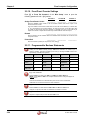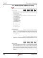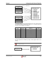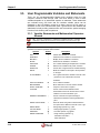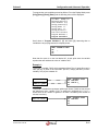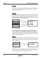
1
Volume 3 Configuration and Advanced Operation CONFIGURATION AND ADVANCED OPERATION Contents of Volume 3 Figures of Volume 3.......................................................................................................viii About Our Company.......................................................................................................... ix Contacting Our Corporate Headquarters ........................................................................ ix Getting User Support ................................................................................................................ ix About the Flow Computer Applications ........................................................................... x About the User Manual....................................................................................................... x Target Audience ........................................................................................................................ x Manual Structure ...................................................................................................................... xi Volume 1. System Architecture and Installation .............................................................. xi Volume 2. Basic Operation .............................................................................................. xi Volume 3. Configuration and Advanced Operation ..........................................................xii Conventions Used in this Manual ............................................................................................xiii Trademark References............................................................................................................xiv Copyright Information and Modifications Policy.......................................................... xiv Warranty, Licenses and Product Registration.............................................................. xiv 1. Overview of Firmware Revisions 23/27 ................................................................ 1-1 1.1. Number of Meter Runs - Type of Flowmeters......................................................1-1 1.2. Product Configuration ...........................................................................................1-1 50-2327-0003 Rev B ® i OMNI 6000 / OMNI 3000 User Manual Contents of Volume 3 1.3. Configurable Sensors per Meter Run................................................................... 1-2 1.4. Temperature, Pressure and Differential Pressure Transmitters........................ 1-2 1.5. Densitometers ........................................................................................................ 1-2 1.6. Gas Chromatographs ............................................................................................ 1-2 1.7. Station Capability................................................................................................... 1-2 1.8. Gas Products - Information Stored / Product...................................................... 1-2 1.9. Type of Gases Measured....................................................................................... 1-2 1.10. Totalizing and Batching ........................................................................................ 1-3 1.11. PID Control Functions ........................................................................................... 1-3 1.12. Master Meter Proving............................................................................................. 1-3 1.13. Time Weighted and Flow Weighted Averages..................................................... 1-3 1.14. User-Programmable Digital I/O ............................................................................. 1-3 1.15. User-Programmable Logic Functions .................................................................. 1-3 1.16. User-Programmable Alarm Functions ................................................................. 1-3 1.17. User-Programmable Variables.............................................................................. 1-4 1.18. User Display Setups .............................................................................................. 1-4 1.19. User Report Templates.......................................................................................... 1-4 1.20. Serial Communication Links................................................................................. 1-4 1.21. Peer-to-Peer Communications.............................................................................. 1-4 1.22. Archive Data ........................................................................................................... 1-4 1.23. OmniCom ® 1.24. OmniView ® Windows Version Software Communications Package ................ 1-5 Window Version Software Communications Package .................. 1-5 1.25. Detailed Daily Report ............................................................................................. 1-5 1.26. Maintenance Mode ................................................................................................. 1-5 1.27. HART Protocol........................................................................................................ 1-5 2. Flow Computer Configuration................................................................................2-1 2.1. Introduction ............................................................................................................ 2-1 2.2. Configuring with the Keypad in Program Mode.................................................. 2-1 2.2.1. Entering the Program Mode ......................................................................................2-1 2.2.2. Changing Data...........................................................................................................2-1 2.2.3. Menu Selection Method .............................................................................................2-2 2.2.4. Random Access Method ...........................................................................................2-3 ® ii 50-2327-0003 Rev B Volume 3 Configuration and Advanced Operation 2.2.5. Passwords .................................................................................................................2-4 2.3. Getting Help ............................................................................................................2-5 2.4. Program Inhibit Switch ..........................................................................................2-6 2.5. Configuring the Physical Inputs / Outputs ..........................................................2-7 2.5.1. Miscellaneous I/O Configuration (Misc. Setup Menu) ...............................................2-8 2.5.2. Physical I/O Points not Available for Configuration ...................................................2-9 2.5.3. Password Maintenance Settings ...............................................................................2-9 2.5.4. Entries Requiring a Valid Privileged Password .......................................................2-10 2.5.5. Module Settings .......................................................................................................2-11 2.5.6. Meter Station I/O Assignments................................................................................2-12 2.5.7. Meter Run I/O Assignments ....................................................................................2-14 2.5.8. PID Control I/O Assignments...................................................................................2-17 2.5.9. Analog Output Assignments ....................................................................................2-19 2.5.10. Front Panel Counter Settings ..................................................................................2-20 2.5.11. Programmable Boolean Statements .......................................................................2-20 2.5.12. Programmable Variable Statements .......................................................................2-23 2.5.13. User Display Settings ..............................................................................................2-26 2.5.14. Digital I/O Point Settings..........................................................................................2-28 Digital I/O Point Settings (continued)....................................................................................2-29 Digital I/O Point Settings (continued)....................................................................................2-30 2.5.15. Serial Input / Output Settings..................................................................................2-31 2.5.16. Custom Modbus™ Data Packet Settings.................................................................2-33 2.5.17. Programmable Logic Controller Setup ....................................................................2-34 2.5.18. Archive File Setup....................................................................................................2-34 2.5.19. Peer-to-Peer Communications Settings ..................................................................2-35 2.5.20. Custom Modbus™ Data Packet Settings.................................................................2-39 2.5.21. Archive File Setup....................................................................................................2-40 2.6. Setting Up The Time and Date ............................................................................2-40 2.6.1. Accessing the Time/Date Setup Submenu..............................................................2-40 2.6.2. Time and Date Settings ...........................................................................................2-40 2.7. Configuring Printers ............................................................................................2-41 2.7.1. Accessing the Printer Setup Submenu....................................................................2-41 2.7.2. Printer Settings ........................................................................................................2-41 2.8. Configuring Gas Chromatograph (GC) Analyzers ............................................2-43 2.8.1. Accessing the Analyzer Setup Submenu ................................................................2-43 2.8.2. Analyzer Settings.....................................................................................................2-43 50-2327-0003 Rev B ® iii OMNI 6000 / OMNI 3000 User Manual Contents of Volume 3 2.9. Configuring Premium Billing Threshold Levels (Revision 23.74/ 75 US Customary Units Only) ........................................................................................ 2-46 2.9.1. Accessing Premium Billing Settings ........................................................................2-46 2.9.2. Premium Billing Threshold Settings.........................................................................2-46 2.10. Configuring PID Control Outputs ....................................................................... 2-47 2.10.1. Accessing the PID Control Setup Submenu............................................................2-47 2.10.2. PID Control Output Settings ....................................................................................2-47 2.11. Configuring Meter Specific Gravity / Density .................................................... 2-49 2.11.1. Accessing the Gravity/Density Setup Submenu......................................................2-49 2.11.2. Meter Specific Gravity / Density Settings ................................................................2-49 2.12. Configuring Meter Temperature ......................................................................... 2-52 2.12.1. Accessing the Temperature Setup Submenu..........................................................2-52 2.12.2. Station and Meter Run Temperature Settings.........................................................2-52 2.12.3. Station and Meter Run Density Temperature Settings............................................2-53 2.13. Configuring Meter Pressure................................................................................ 2-54 2.13.1. Accessing the Pressure Setup Submenu................................................................2-54 2.13.2. Station and Meter Run Pressure Settings ...............................................................2-54 2.13.3. Station and Meter Run Density Pressure Settings ..................................................2-55 2.14. Configuring Differential Pressure....................................................................... 2-57 2.14.1. Accessing the Differential Pressure Setup Submenu .............................................2-57 2.14.2. Station and Meter Differential Pressure Settings ....................................................2-57 2.15. Configuring the Meter Station............................................................................. 2-59 2.15.1. Accessing the Station Setup Submenu ...................................................................2-59 2.15.2. Meter Station Settings .............................................................................................2-59 2.16. Configuring Meter Runs ...................................................................................... 2-63 2.16.1. Accessing the Meter Run Setup Submenu .............................................................2-63 2.16.2. Meter Run Settings ..................................................................................................2-63 2.17. Configuring Miscellaneous Factors ................................................................... 2-68 2.17.1. Accessing the Factor Setup Submenu ....................................................................2-68 2.17.2. Factor Settings.........................................................................................................2-68 2.18. Configuring Fluid Data and Analysis of Products ............................................ 2-70 2.18.1. Accessing the Fluid Data & Analysis Setup Submenu ............................................2-70 2.18.2. General Fluid Data & Analysis (Product) Settings...................................................2-70 2.18.3. Additional Settings for Natural Gas Product............................................................2-72 2.19. Configuring Prover .............................................................................................. 2-75 2.19.1. Accessing the Prover Setup Submenu....................................................................2-75 ® iv 50-2327-0003 Rev B Volume 3 Configuration and Advanced Operation 2.19.2. Prover Settings ........................................................................................................2-75 3. User-Programmable Functions ............................................................................. 3-1 3.1. Introduction ............................................................................................................3-1 3.2. User-Programmable Boolean Flags and Statements..........................................3-1 3.2.1. What is a Boolean?....................................................................................................3-1 3.2.2. Sign (+, -) of Analog or Calculated Variables 3.2.3. Boolean Statements and Functions ..........................................................................3-3 3.2.4. How the Digital I/O Assignments are Configured ......................................................3-8 (5001 → 8999)..............................3-3 3.3. User Programmable Variables and Statements ................................................3-10 3.3.1. Variable Statements and Mathematical Operators Allowed....................................3-10 3.3.2. Using Boolean Variables in Variable Statements....................................................3-12 3.3.3. Entering Values Directly into the User Variables.....................................................3-13 3.3.4. Using the Variable Expression as a Prompt............................................................3-13 3.3.5. Password Level Needed to Change the Value of a User Variable .........................3-13 3.3.6. Using Variables in Boolean Expressions.................................................................3-14 3.4. User Configurable Display Screens ...................................................................3-15 4. Flow Equations and Algorithms for U.S. Customary Units (Revision 23.74/75) 4-1 4.1. Flow Rate for Gas Differential Pressure Devices (Orifice, Nozzle and Venturi)4-1 4.1.1. Mass Flow Rate at Flowing Conditions ‘Qm’ (Klbm/hr) ..............................................4-1 4.1.2. Volumetric Gross Flow Rate at Flowing Conditions ‘Qv’ (MCF/hr) ............................4-1 4.1.3. Volumetric Net Flow Rate at Base Conditions ‘Qb’ (MSCF/hr)..................................4-2 4.1.4. Energy Flow Rate at Base Conditions ‘Qe’ (MMBTU/hr) ...........................................4-2 4.1.5. Nomenclature ............................................................................................................4-2 4.1.6. Diameters and Diameter Correlations .......................................................................4-3 4.1.7. Velocity of Approach Factor ‘Ev’................................................................................4-5 4.1.8. Discharge Coefficients ‘Cd’ ........................................................................................4-6 4.1.9. Fluid Expansion Factor Referenced to Upstream Pressure ‘Y1’.............................4-10 4.2. Flow Rate for Gas Turbine Flowmeters..............................................................4-12 4.2.1. Volumetric Gross Flow Rate at Flowing Conditions ‘QV’ (MCF/hr)..........................4-12 4.2.2. Mass Flow Rate at Flowing Conditions ‘Qm’ (Klbm/hr) ............................................4-12 4.2.3. Volumetric Net Flow Rate at Base Conditions ‘Qb’ (MSCF/hr)................................4-12 4.2.4. Energy Flow Rate at Base Conditions ‘Qe’ (MMBTU/hr) .........................................4-12 50-2327-0003 Rev B ® v OMNI 6000 / OMNI 3000 User Manual 4.2.5. Contents of Volume 3 Nomenclature ..........................................................................................................4-13 4.3. Flow Rate for Gas Coriolis Flowmeters ............................................................. 4-14 4.4. Densities and Other Properties of Gas .............................................................. 4-15 4.4.1. AGA Report NO 8: Compressibility for Natural Gas and Other Related Hydrocarbon Gases.......................................................................................................................4-15 4.4.2. ASME 1967 Steam Equation ‘υr’ .............................................................................4-19 4.4.3. Water Density ..........................................................................................................4-19 4.4.4. NBS Density (lb/CF), Viscosity Isentropic Exponent, Sound Velocity, and Enthalpy4-19 4.4.5. Density and Relative Density (Specific Gravity) Calculated from Digital Densitometer and Gravitometer Output Frequency .......................................................................4-20 5. Flow Equations and Algorithms for S.I. (Metric) Units (Revision 27.74/75) .......5-1 5.1. Flow Rate for Gas Differential Pressure Devices (Orifice, Nozzle and Venturi)5-1 5.1.1. Mass Flow Rate at Flowing Conditions ‘Qm’ (Tonnes/hr) ..........................................5-1 5.1.2. Volumetric Gross Flow Rate at Flowing Conditions ‘Qv’ (m3/hr)................................5-1 5.1.3. Volumetric Net Flow Rate at Base Conditions ‘Qb’ (m3/hr)........................................5-2 5.1.4. Energy Flow Rate at Base Conditions ‘Qe’ (GJ/hr)....................................................5-2 5.1.5. Nomenclature ............................................................................................................5-2 5.1.6. Diameters and Diameter Correlations .......................................................................5-3 5.1.7. Coefficient of Discharge ‘C’ .......................................................................................5-5 5.1.8. Fluid Expansion Factor ‘ε’..........................................................................................5-8 5.2. Flow Rate for Gas Helical Turbine Flowmeters................................................... 5-9 5.2.1. Volumetric Gross Flow Rate at Flowing Conditions ‘QV’ (m3/hr) ...............................5-9 5.2.2. Mass Flow Rate at Flowing Conditions ‘Qm’ (Tonnes/hr) ..........................................5-9 5.2.3. Volumetric Net Flow Rate at Base Conditions ‘Qb’ (m3/hr)........................................5-9 5.2.4. Energy Flow Rate at Base Conditions ‘Qe’ (GJ/hr)....................................................5-9 5.2.5. Nomenclature ..........................................................................................................5-10 5.3. Flow Rate for Gas Coriolis Flowmeters ............................................................. 5-11 5.4. Densities and Other Properties of Gas .............................................................. 5-12 5.4.1. AGA Report NO 8: Compressibility for Natural Gas and Other Related Hydrocarbon Gases.......................................................................................................................5-12 5.4.2. ASME 1967 Steam Equation ‘υr’ .............................................................................5-16 5.4.3. Water Density ..........................................................................................................5-16 5.4.4. NBS Density, Viscosity Isentropic Exponent, Sound Velocity, and Enthalpy..........5-16 5.4.5. Density and Relative Density (Specific Gravity) Calculated from Digital Densitometer and Gravitometer Output Frequency .......................................................................5-17 ® vi 50-2327-0003 Rev B Volume 3 Configuration and Advanced Operation 5.4.6. 50-2327-0003 Rev B NX19 Analysis (1980 Edition)..................................................................................5-21 ® vii OMNI 6000 / OMNI 3000 User Manual Contents of Volume 3 Figures of Volume 3 Figure. 1-1. Typical Gas Flow Metering Configuration with Turbine and OrificeFlowmeters…1-1 Figure. 2- Figure Showing Program Inhibit Switch ...................................................................2-6 Figure. 3-1. Figure Showing Automatic Four-Meter Flow Zone Thresholds ...............................3-6 Figure. 3-2. Figure Showing Four-Meter Run Valve Switching ...................................................3-7 Figure. 3-3. Keypad Layout - A through Z Keys ........................................................................3-16 ® viii 50-2327-0003 Rev B Volume 3 Configuration and Advanced Operation About Our Company Measure the Difference!® OMNI Flow Computers, Inc. is the world’s leading manufacturer and supplier of panel-mount custody transfer flow computers and controllers. Our mission is to continue to achieve higher levels of customer and user satisfaction by applying the basic company values: our people, our products and productivity. OMNI Flow Computers – Our products are currently being used world-wide at: 9 Offshore oil and gas production facilities 9 Crude oil, refined products, LPG, NGL and gas transmission lines 9 Storage, truck, and marine loading/offloading terminals 9 Refineries; petrochemical and cogeneration plants Our products have become the international flow computing standard. OMNI Flow Computers pursues a policy of product development and continuous improvement. As a result, our flow computers are considered the “brain” and “cash point” of liquid and gas flow metering systems. Our staff is knowledgeable and professional. They represent the energy, intelligence and strength of our company, adding value to our products and services. With the customer and user in mind, we are committed to quality in everything we do, devoting our efforts to deliver workmanship of high caliber. Teamwork with uncompromising integrity is our lifestyle. Contacting Our Corporate Headquarters OMNI Flow Computers, Inc. 12620 West Airport Suite 100 Sugar Land, Texas 77478 USA Phone: 281-240-6161 Fax: 281-240-6162 World-wide Web Site: http://www.omniflow.com O E-mail Addresses: [email protected] Getting User Support Technical and sales support is available world-wide through our corporate or authorized representative offices. If you require user support, please contact the location nearest you (see insert) or our corporate offices. Our staff and representatives will enthusiastically work with you to ensure the sound operation of your flow computer. 50-2327-0003 Rev B ® ix OMNI 6000 / OMNI 3000 User Manual For Your Information About the Flow Computer Applications OMNI 6000 and OMNI 3000 Flow Computers are integral into the majority of liquid and gas flow measurement and control systems. The current firmware revisions of OMNI 6000/OMNI 3000 Flow Computers are: • 23/27: units) Orifice/Turbine Gas Flow Metering Systems (US/metric About the User Manual This manual applies to 23/27 firmware revisions of OMNI 6000 and OMNI 3000 Flow Computers. It is structured into 5 volumes and is the principal part of your flow computer documentation. Target Audience As a user’s reference guide, this manual is intended for a sophisticated audience with knowledge of liquid and gas flow measurement technology. Different user levels of technical know-how are considered in this manual. You need not be an expert to operate the flow computer or use certain portions of this manual. However, some flow computer features require a certain degree of expertise and/or advanced knowledge of liquid and gas flow instrumentation and electronic measurement. In general, each volume is directed towards the following users: • Volume 1. System Architecture and Installation ♦ Installers ♦ System/Project Managers ♦ Engineers/Programmers ♦ Advanced Operators ♦ Operators • Volume 2. Basic Operation ♦ All Users • Volume 3. Configuration and Advanced Operation ♦ Engineers/Programmers ♦ Advanced Operators • Volume 4. Modbus™ Database Addresses and Index Numbers ♦ Engineers/Programmers ♦ Advanced Operators • Volume 5. Technical Bulletins ♦ Users with different levels of expertise. ® x 50-2327-0003 Rev B Volume 3 Configuration and Advanced Operation Manual Structure The User Manual comprises 5 volumes; each contained in separate binding for easy manipulation. You will find a detailed table of contents at the beginning of each volume. The User Manual comprises 5 volumes; each contained in separate binding for easy manipulation. You will find a detailed table of contents at the beginning of each volume. User Reference Documentation – The User Manual is structured into five volumes. Volumes 1, 2, and 5 are generic to all flow computer application revisions. Volumes 3 and 4 are application specific. These have four versions each, published in separate documents; i.e., one per application revision per volume. You will receive the version that corresponds to your application revision. The volumes respective to each application revision are: Revision 23/27: Volume #s 3, 4 Volume 1. System Architecture and Installation Volume 1 is generic to all applications and considers both US and metric units. This volume describes: * * * * Basic hardware/software features Installation practices Calibration procedures Flow computer specifications Volume 2. Basic Operation This volume is application specific and is available in four separate versions (one for each application revision). It covers the essential and routine tasks and procedures that may be performed by the flow computer operator. Both US and metric units are considered. General computer-related features are described, such as: * * * * * Overview of keypad functions Adjusting the display Clearing and viewing alarms Computer totalizing Printing and customizing reports The application-related topics may include: * * * * * Batching operations Proving functions PID control functions Audit trail Other application specific functions Depending on your application, some of these topics may not be included in your specific documentation. An index of display variables and corresponding key press sequences that are specific to your application are listed at the end of each version of this volume. 50-2327-0003 Rev B ® xi OMNI 6000 / OMNI 3000 User Manual For Your Information Volume 3. Configuration and Advanced Operation Volume 3 is intended for the advanced user. It refers to application specific topics and is available in four separate versions (one for each application revision). This volume covers: * Application overview * Flow computer configuration data entry * User-programmable functions * Modbus™ Protocol implementation Flow equations and algorithms Volume 4. Modbus™ Database Addresses and Index Numbers Volume 4 is intended for the system programmer (advanced user). It comprises a descriptive list of database point assignments in numerical order, within our firmware. This volume is application specific, for which there is one version per application revision. Volume 5. Technical Bulletins Manual Updates and Technical Bulletins – Volume 5 of the User Manual is a compendium of Technical bulletins. You can view and print technical bulletins from our website: http://www.omniflow.com Volume 5 includes technical bulletins that contain important complementary information about your flow computer hardware and software. Each bulletin covers a topic that may be generic to all applications or specific to a particular revision. They include product updates, theoretical descriptions, technical specifications, procedures, and other information of interest. This is the most dynamic and current volume. Technical bulletins may be added to this volume after its publication. ® xii 50-2327-0003 Rev B Volume 3 Configuration and Advanced Operation Conventions Used in this Manual Several typographical conventions have been established as standard reference to highlight information that may be important to the reader. These will allow you to quickly identify distinct types of information. CONVENTION USED DESCRIPTION The light bulb icon indicates a tip, suggestion, or concise information of interest. It is highly recommended that you read them. Keys / Key press Sequences Example: [Prog] [Batch] [Meter] [n] Keys on the flow computer keypad are denoted with brackets and bold face characters (e.g.: the ‘up arrow’ key is denoted as [Ç]). The actual function of the key as it is labeled on the keypad is what appears between brackets. Key press sequences that are executed from the flow computer keypad are expressed in a series of keys separated by a space (as shown in the example). Screen Displays Example: Use Up/Down Arrows To Adjust Contrast; Left, Right Arrows To Adjust Backlight Headings Example: 2. Chapter Heading 2.3. Section Heading Sample screens that correspond to the flow computer display appear surrounded by a dark gray border with the text in bold face characters and mono-spaced font. The flow computer display is actually 4 lines by 20 characters. Screens that are more than 4 lines must be scrolled to reveal the text shown in the manual. Sequential heading numbering is used to categorize topics within each volume of the User Manual. The highest heading level is a chapter, which is divided into sections, which are likewise subdivided into subsections. Among other benefits, this facilitates information organization and cross-referencing. 2.3.1. Subsection Heading Figure Captions Example: Figure. 2-3. Figure No. 3 of Chapter 2 Page Numbers Example: 2-8 50-2327-0003 Rev B Figure captions are numbered in sequence as they appear in each chapter. The first number identifies the chapter, followed by the sequence number and title of the illustration. Page numbering restarts at the beginning of every chapter and technical bulletin. Page numbers are preceded by the chapter number followed by a hyphen. Technical bulletins only indicate the page number of that bulletin. Page numbers are located on the outside margin in the footer of each page. ® xiii OMNI 6000 / OMNI 3000 User Manual For Your Information Trademark References The following are trademarks of OMNI Flow Computers, Inc.: • OMNI 3000 • OMNI 6000 • OmniCom® Other brand, product and company names that appear in this manual are trademarks of their respective owners. Copyright Information and Modifications Policy This manual is copyright protected. All rights reserved. No part of this manual may be used or reproduced in any form, or stored in any database or retrieval system, without prior written consent of OMNI Flow Computers, Inc., Sugar Land, Texas, USA. Making copies of any part of this manual for any purpose other than your own personal use is a violation of United States copyright laws and international treaty provisions. OMNI Flow Computers, Inc., in conformance with its policy of product development and improvement, may make any necessary changes to this document without notice. Warranty, Licenses and Product Registration Product warranty and licenses for use of OMNI flow computer firmware and of OmniCom Configuration PC Software are included in the first pages of each Volume of this manual. We require that you read this information before using your OMNI flow computer and the supplied software and documentation. Important! If you have not done so already, please complete and return to us the product registration form included with your flow computer. We need this information for warranty purposes, to render you technical support and serve you in future upgrades. Registered users will also receive important updates and information about their flow computer and metering system. Copyright ©1991-2009 by OMNI Flow Computers, Inc. All Rights Reserved. ® xiv 50-2327-0003 Rev B Volume 3 Configuration and Advanced Operation 1. Overview of Firmware Revisions 23/27 Orifice / Turbine / Coriolis/ Ultrasonic Gas Flow Metering Systems 1.1. Number of Meter Runs - Type of Flowmeters Minimum 1 run, maximum 4 runs – Typical gas orifice meter run shown. 1.2. Product Configuration Parallel runs measuring the same product or independent runs with different products. TURBINE/MASS/ ULTRASONIC METERS ORIFICE METERS FT FT FT FT Figure. 1-1. Typical Gas Flow Metering Configuration Using Turbine / Coriolis/Ultrasonic and Orifice Flowmeters 50-2327-0003 Rev B ® 1-1 Chapter 1 1.3. Overview of Firmware Revisions 23.74/27.74 Configurable Sensors per Meter Run Meter turbines, differential pressures, Rosemount Multivariable DP, Honeywell Multivariable DP, Instroment Qsonic, V-Cone Flowmeter, FMC MPU1200, Equimeter AAT, Daniel Ultransonic, Coriolis Meter, FlowSic 600 Ultrasonic, meter temperature and pressure, meter density, density temperature and pressure. 1.4. Temperature, Pressure and Differential Pressure Transmitters All transmitters can be 4-20mA, 1-5V or Honeywell DE digital protocol types. In addition temperature sensors can also be four wire DIN or American curve RTD probes connected directly. 1.5. Densitometers Can be configured for any combination or mix of individual or shared densitometers of any type (analog specific gravity, analog density, digital Solartron pulse, digital Sarasota pulse or digital UGC pulse); the maximum number that can be connected is four. 1.6. Gas Chromatographs Where applicable, analysis data can be obtained automatically via a serial communication port from a gas chromatograph. Standard protocols communicate with (1) Applied Automation™ analyzers, (2) Daniels™ Danalyzer, (3) other analyzers which communicate using Modbus™ protocol. It is now possible to read two independent Gas Chromatographs streams via the third serial port. 1.7. Station Capability Meter runs may be combined or subtracted in any mode to provide station flow rates and totalizers. Can be used in 'Check /Pay' meter systems to monitor flows and alarm if deviations exceed a preset limit. 1.8. Gas Products - Information Stored / Product Information for four different gases can be stored. Product setup information includes: name, type of gas, component analysis, relative density at reference conditions and calculation algorithm to be used when running the product. 1.9. Type of Gases Measured Natural gas and other fluids covered by: AGA 3 1992; API 14.3; AGA 8 Reports 1994, 1992 and 1985; ASTM Steam; NIST Steam, Water, Argon, Nitrogen, Oxygen, paraHydrogen, and Ethylene using NIST 1048. ® 1-2 50-2327-0003 Rev B Volume 3 Configuration and Advanced Operation 1.10. Totalizing and Batching Gross (uncorrected) volume, Net (standard conditions) volume, Mass and Energy totalizers are provided for each meter run and defined station group. Separate totalizer sets provide, Cumulative (non resettable) Daily and Batch totalizers. The Batch totalizers can be used to provide either weekly, monthly or on demand totalizing information. 1.11. PID Control Functions Four independent control loops are provided for control of a primary variable with either high or low override control by a secondary variable. Contact closure inputs are activated to provide a startup ramp function for each control loop if needed. Primary set point can be adjusted via an analog input, a keypad entry or communication link. Control loops are not dedicated and may be cascaded. Data is processed every 500 msec. 1.12. Master Meter Proving Master Meter proving has been added. Meter I/O point #4 has to be setup as the Master Meter Input. 1.13. Time Weighted and Flow Weighted Averages Either Flow weighted or time weighted averages for all input variables and correction factors based on daily flow or batch flow are standard. Because errors such as entering an incorrect orifice diameter, would cause large flow errors and errors in the flow weighted averages, time weighted averages are calculated for orifice metering runs. Averaging does not occur if the flow rate is zero. All variables associated with Turbine metering runs are flow weighted averaged. Gas chromatograph data is always time weighted. 1.14. User-Programmable Digital I/O Each I/O point is individually configurable as either an input or output with variable 'delay On' and 'delay Off'. Pulse widths are adjustable when used as auxiliary totalizer outputs or sampler outputs. 1.15. User-Programmable Logic Functions Sixty-four logic statements can be user programmed to control meter run switching and provide user auxiliary control functions. 1.16. User-Programmable Alarm Functions Sixteen of the programmable logic statements described above can be used to contain custom text messages which can be displayed, logged and printed. 50-2327-0003 Rev B ® 1-3 Chapter 1 Overview of Firmware Revisions 23.74/27.74 1.17. User-Programmable Variables Sixty-four user variables can be programmed to manipulate data for display and printing or remote access via a communication port. Typical uses include, special units conversions, customer averaging algorithms for leak detection, special limit checking and control functions. The programmable variable statements can also be used to type cast data of one type to another (i.e., change a floating point variable to an integer type so that a PLC or DCS system can make use of it). 1.18. User Display Setups The user may specify eight key press combinations which recall display screens. Each user display screen can show four variables each with a descriptive tag defined by the user. 1.19. User Report Templates Using OmniCom the user can generate custom report templates or edit existing templates. These are uploaded into the flow computer. Custom templates for the snapshot, batch end, daily and prove reports can be defined. 1.20. Serial Communication Links Up to six serial data links are available for communications with other devices such as printers, SCADA systems, PLC’s and other OMNI Flow Computers. Ports communicate using a superset of the Modbus™ protocol (ASCII or RTU). Printer data is ASCII data. Ethernet communications are also available. Up to two modules per system can be used. 1.21. Peer-to-Peer Communications OMNI flow computers can be user configured to communicate with each other as equal peers. Groups of data variables can be exchanged or broadcast between other flow computers. Multiple flow computers can share resources such as a PLC. 1.22. Archive Data Two types of data archiving are possible in the flow computer. (1) Formatted ASCII text using custom report templates, (2) Raw Data using archive records and files. ® 1-4 50-2327-0003 Rev B Volume 3 Configuration and Advanced Operation 1.23. OmniCom® Windows Version Software Communications Package OmniCom® Windows version software is provided with each flow computer, and allows the user to configure the computer on-line or off-line using a personal computer. 1.24. OmniView® Window Version Software Communications Package A Man-Machine Interface package for the OMNI Flow Computer is also available as an option. 1.25. Detailed Daily Report A Detailed Daily report has been added for the user to select. The computer stores 35 days configuration data of each meter run for this report. The data includes low flow cutoff, viscosity, isentropic expansion factor, pipe diameter at reference temperature, orifice diameter at reference temperature, density of air, base temperature, base pressure atmospheric pressure and the daily average of water content. See under ‘Password Maintenance” for associated entry. To print the report Press ‘Prog’ ‘Print’ ‘Enter and scroll down to the entry (which must be activated under the Password Menu screen) to display ‘Meter # Detail Report and enter the meter number to print the report. 1.26. Maintenance Mode Totalizer Maintenance Mode has been added to firmware 23.74.30 and 27.74.30. For additional help see technical bulletin 52-0000-0010 (TB980701). 1.27. HART Protocol Firmware version 23/27.75 can now accept HART enabled devices (Differental Pressure, Temperature or Pressure transmitters) communication. The user can now configure the HART enabled devices thru the use of a new I/O module which can be setup as a HT or HM module. See Technical Bulletin 52-00000019 (TB090003) for additional information. 50-2327-0003 Rev B ® 1-5 Chapter 1 Overview of Firmware Revisions 23.74/27.74 This page left intentionally blank. ® 1-6 50-2327-0003 Rev B Volume 3 Configuration and Advanced Operation 2. Flow Computer Configuration 2.1. Introduction Configuration data is stored in the computer's battery backed-up RAM memory which will retain its data for at least 1 to 2 months with no power applied. Configuration data can be entered using one of three methods: 1) Configure off-line using the OmniCom PC configuration program and then uploading all data at once. 2) Configure on-line using the OmniCom PC configuration program which uploads each change as it is entered. 3) Enter configuration data via the front panel keypad using the Program Mode. Methods 1) and 2) require an IBM compatible PC running the OmniCom Configuration Software and are described in Volume 5 and in OmniCom Help. Method 3) is described here. 2.2. Configuring with the Keypad in Program Mode 2.2.1. Entering the Program Mode INFO: Key presses are denoted in bold face between brackets; e.g.: the enter key appears in this manual as [Enter]. While in the Display Mode press the [Prog] key. The front panel Program LED above the key will glow green and the following selection menu will be displayed on the first three lines of the LCD display. The 4th line of the display is used to show the user key presses. Press Keys to Select Group Entry, or Press "Prog" to Exit 2.2.2. Changing Data Data can be accessed using a sequential list of menu prompts or in a random access manner by going directly to a specific group of entries. 50-2327-0003 Rev B ® 2-1 Chapter 2 Flow Computer Configuration 2.2.3. Menu Selection Method INFO: Characters in ‘[ ]’ refer to key presses. TIP: It is best to use the menu selection method when programming an application for the first time as every possible option and variable will be prompted. Once a computer is in operation and you become familiar with the application you can decide to use the faster Random Access Method. To use the menu selection method, while in the Program Mode (program LED on) press [Setup] [Enter]. A Setup Menu similar to the one on the right will be displayed *** SETUP MENU *** Misc Configuration _ Time/Date Setup Printer Setup Analyser Setup PID Control Setup Grav/Density Setup Temperature Setup Pressure Setup DP Inches of Water Prover Setup Station Setup Meter Run Setup Factor Setup FluidData&Analysis Use the [Ç]/[È] (up/down arrow) keys to move the cursor to the appropriate entry and press [Enter] to access a particular submenu. The first menu, 'Misc Configuration', should always be completed first as these entries specify the number and type of input and output devices connected to the flow computer; i.e., the menus following the 'Misc Configuration' menu do not ask for configuration data unless a transducer has been defined. ® 2-2 50-2327-0003 Rev B Volume 3 Configuration and Advanced Operation 2.2.4. Random Access Method In addition to the Setup Menu, the data is also presented in related groups such as Temperature, Pressure, Meter, etc. You press the group key of your choice to get to a data area. By specifying a meter run before or after a group you go directly to the data for that group and that group only. Once a group is selected use the 'Up/Down' arrow keys to step to a specific data entry within the group. You can view data and, assuming a valid password has been entered, change its value as required. If an error is made, press [Clear], re-enter the correct data and press [Enter] to enter the new value. The cursor will automatically step to the next data item in that group unless that would cause a total change of screen (i.e., you can always verify your entry). A list of data groups and associated key presses is listed later in this chapter. Example: Pressing [Temp] will allow you access to temperature data for all meter runs. Pressing [Meter] [1] [Temp] or [Temp] [Meter] [1] will allow access to only Meter Run #1 temperature data. For example, pressing [Meter] [1] [Temp] will display the following until the [Enter] key is pressed. Press Keys to Select Group Entry, or Press "Prog" to Exit Meter 1 Temp Pressing the [Enter] key will display a screen similar to this: TEMPERATURE #1 Deg.F Low Limit 30.0 High Limit 125.0 Override 60.0 50-2327-0003 Rev B ® 2-3 Chapter 2 Flow Computer Configuration 2.2.5. Passwords INFO: Most entry groups occupy multiple screens so be sure to use the [Ç]/[È] to scroll and see all data. Except when changing transducer high/low alarm limits, a password is usually asked for when changing the configuration data within the computer. The flow computer has independent password protection of the following: • • Local Keypad Access / Modbus Port #1 (selectable) (Physical Serial Port #1) • Modbus Port #2 - (Physical Serial Port #2) • Modbus Port #3 - (Physical Serial Port #3) • Modbus Port #4 - (Physical Serial Port #4) Local Keypad Access Three password levels are provided: • Privileged Level Allows complete access to all entries within the flow computer including keypad passwords 1, 1A and 2 below. The initial privileged password for each Modbus port is selected via this password level. • Level 1 This level allows technician access to most entries within the flow computer with the exception of I/O Points assignments, programmable variables and Boolean statements and passwords other than ‘Keypad Level 1’. • Level 1A This level allows technician access to the following entries only: ♦ Meter Factors ♦ K Factors ♦ Densitometer Correction Factors (Pycnometer Factor) • Level 2 Allows access to the operator type entries. These entries include: ♦ ♦ ♦ ♦ Transducer Manual Overrides Product Gravity Overrides Prove Operations Batching Operations ® 2-4 50-2327-0003 Rev B Volume 3 Configuration and Advanced Operation Changing Passwords at the Keypad INFO: Characters in ‘[ ]’ refer to key presses. 1) At the keypad press [Prog] [Setup] [Enter]. 2) With the cursor blinking on 'Misc Configuration', press [Enter]. 3) With the cursor blinking on 'Password Maint?', press [Enter]. 4) Enter the Privileged Level Password (up to 6 Characters) and press [Enter]. 5) The Level 1, 1A and Level 2 passwords can now be viewed and changed if required. 6) Scroll down to access each of the Modbus serial port 'Level A' passwords. These are labeled ‘Serial 1’ (if Modbus Protocol is selected), 'Serial 2', Serial 3', and 'Serial 4' corresponding to the physical port numbering for Modbus Ports 1, 2, 3 and 4. INFO: See Technical Bulletin 52-0000-0001 (TB-960701) in Volume 5 for setting Level B and Level C passwords using OmniCom. NOTE: Level B and Level C passwords for each Modbus port cannot be viewed or changed from the keypad INFO: The Help System is not limited to just the Program Mode. Context sensitive help is available in all modes of operation 2.3. Getting Help Context sensitive help is available for most data entries. Help is summoned by pressing the [Display/Enter] key twice ([Help] key) with the cursor on the data field in question. Help screens are frequently more than 1 full screen so always use the [Ç]/[È] keys to scroll in case there is more. Press [Prog] or [Enter] once to exit the help system and return to your original screen. 50-2327-0003 Rev B ® 2-5 Chapter 2 Flow Computer Configuration 2.4. Program Inhibit Switch A 'Program Inhibit Switch' mounted behind the front panel prevents unauthorized changing of data when in the 'Inhibit' position. Most data can be viewed while the switch is in the program inhibit position, but any attempt to alter data will be ignored and cause 'PROGRAM LOCKOUT' to be displayed on the bottom line of the LCD display. The inner enclosure of the flow computer can be locked or sealed within the outer enclosure blocking access to the 'Program Inhibit Switch'. CAUTION! These units have an integral latching mechanism which first must be disengaged by lifting the bezel upwards before withdrawing the unit from the case. Figure. 2-1. Figure Showing Program Inhibit Switch ® 2-6 50-2327-0003 Rev B Volume 3 Configuration and Advanced Operation 2.5. Configuring the Physical Inputs / Outputs TIP: It is best to use the Menu Selection Method (see 2.2.3, this chapter) when programming an application for the first time as every possible option and variable will be prompted. Once a computer is in operation and you become familiar with the application you can decide to use the faster Random Access Method (see 2.2.4, this chapter) INFO: Characters in ‘[ ]’ refer to key presses INFO: The first menu, 'Misc Configuration', should always be completed first as these entries specify the number and type of input and output devices connected to the flow computer. You are advise to complete all entries under this menu before proceeding. Only transducers that have been assigned to physical I/O points will be available for further configuration (i.e., the menus following the 'Misc Configuration' menu do not ask for or accept configuration data unless a transducer has been defined). (See 2.5.2, this chapter) The OMNI Flow Computer can accept many I/O modules and be configured to match just about any combination of measurement transmitters. Configuring the physical I/O means setting up the number of meter runs, what types of transducers are to be used and to which physical I/O points they are connected. 50-2327-0003 Rev B ® 2-7 Chapter 2 Flow Computer Configuration 2.5.1. Miscellaneous I/O Configuration (Misc. Setup Menu) The physical I/O configuration of the flow computer is changed by entering the ‘Misc. Setup’ menu while the 'Select Group Entry' screen is displayed (see 9.2.1. “Entering the Program Mode” Press Keys to Select Group Entry, or Press "Prog" to Exit Setup Press [Setup] then [Enter] and the following selection menu will be displayed: *** SETUP MENU *** Misc Configuration _ Time/Date Setup Station Setup The cursor automatically appears at the ‘Misc Configuration’ option. Press [Enter] and the following selection menu will be displayed: *** Misc. Setup *** Password Maint?(Y) Check Modules ?(Y) Config Station?(Y) Config Meter “n” Config PID ? “n” Config D/A Out“n” Front Pnl Counters Program Booleans ? Program Variables? User Display ? “n” Config Digital“n” Serial I/O “n” Peer/Peer Comm(Y)? Custom Packet “n” Archive File “n” ® 2-8 50-2327-0003 Rev B Volume 3 Configuration and Advanced Operation 2.5.2. Physical I/O Points not Available for Configuration Configuration parameter groups are only prompted as needed. Meter runs and transducers which are not assigned to a physical I/O point will not be available for configuration. In these cases the following message will be displayed: If this message is displayed, check the I/O point assignment for the variable. Variable Selected is Not Assigned to a Physical I/O Point 2.5.3. Password Maintenance Settings Password maintenance settings can only be entered via the OMNI front panel keypad. Enter [Y] at ‘Password Maint ?’ of the ‘Misc Setup’ menu to open the following entries: INFO: Characters in ’{ }’ refer to password levels. Characters in ‘[ ]’ refer to key presses. TIP: Use the blank lines provided next to each configuration option to write down the corresponding settings you entered in the flow computer. Some of these entries may not appear on the display or in OmniCom. Depending on the various configuration settings of your specific metering system, only those configuration options which are applicable will be displayed {PL} Privileged _______________ Enter the privileged password to allow you to view and change all configuration data including other passwords. {PL} Level 1 _______________ Enter the Level 1 password to allow entry of all configuration data except entries which determine the physical I/O personality of the computer. {PL} Level 1A _______________ Enter the Level 1A password to allow entry of Meter factors, K Factors and Density Correction Factors only. {PL} Level 2 _______________ Enter the Level 2 password which is required for operator type entries such as gravity overrides and meter factors. {PL} Serial Port #1 Password _______________ Enter the Serial Port password. All data in the Modbus database except passwords can be read via the serial ports. These passwords allow writes to the Modbus database. Password protection can be disabled by entering a blank field as a password. {PL} Lockout Switch Active? (Serial Port #1) _______________ Enter [N] for the lockout switch to be inactive for this serial port. Enter [Y] for the lockout switch to be active for this serial port. {PL} Serial Port #2 Password _______________ Enter the Serial Port #2 Password. 50-2327-0003 Rev B {PL} Lockout Switch Active? (Serial Port #2) _______________ {PL} Serial Port #3 Password _______________ ® 2-9 Chapter 2 Flow Computer Configuration {PL} Lockout Switch Active? (Serial Port #3) _______________ {PL} Serial Port #4 Password _______________ {PL} Lockout Switch Active? (Serial Port #4) _______________ {PL} Serial Port #5 Password _______________ {PL} Lockout Switch Active? (Serial Port #5) _______________ {PL} Serial Port #6 Password _______________ {PL} Lockout Switch Active? (Serial Port #6) _______________ 2.5.4. Entries Requiring a Valid Privileged Password The following entries display only when a Valid Privileged Password is entered: {PL} Model Number (0=3000, 1=6000) _______________ This entry is used by the OmniCom configuration software to determine the maximum I/O capability of the computer. {PL} Disable Download? _______________ Enter ‘Y’ to prevent OmniCom from downloading the configuration file to the OMNI Flow Computer. {PL} Re-configure Archive _______________ Enter [Y] to re-configure archive records definition. Enter [N] when finished. {PL} Archive Run (Y/N) _______________ Enter [Y] to start the archive running. CAUTION! If you change the number or type of installed I/O modules, you must perform the ‘Check Modules’ Function to inform the computer that you wish to use the new hardware configuration. {PL} Start Screen Default (Y/N) _______________ Enter [Y/N] for the computer to return to the last viewed display after a reset or power down Default is N. If using default, user must review historical alarm for any system fail codes. {PL} Dual Pulse Comparison Delay Cycle 0-20 _______________ Maximum threshold and dual pulse delay cycle. Dual Pulse Comparison will be activated when the accumulated error counts exceed this number. For the delay cycle enter 0-20 as the number of 500ms cycle delays, differentiate between simultaneous noise with A=0 and a A failure {PL} Activated Detailed Daily Report ? _______________ Enter Y to activate a Detailed Daily Report within the Flow Computer. ® 2-10 50-2327-0003 Rev B Volume 3 Configuration and Advanced Operation {PL} Reset All Totalizers? (Y/N) _______________ Entering Y will reset all current meter totalizers to 0.0. Once this has been done the user will see another display “ All Totalizers now reset” and the user can now select the totalizers resolution # of digits, 0=9, 1=8. Next the user can select the decimal place resolution for the front panel by selecting the number of decimal places required for Gross, Net and Mass. The three electromechanical totalizers on the front of the computer cannot be zeroed. {PL} Reset All RAM? (Y/N) _______________ Resetting all RAM will clear all configuration data, calibration data and totalizers. This means that all configuration data will have to be re-entered. {PL} Input Calibrate Default? _______________ Entering a [Y] here will set all the analog input calibration constants used to scale zero and span settings to the default value. This will require you to re calibrate all the inputs. You can also do this on a channel by channel basis by entering the input channel number. {PL} D/A Calibrate Default? _______________ Entering a [Y] here will set all the analog output calibration constants used to scale zero and span settings to the default value. This will require you to re-calibrate all the outputs. You can also do this on a channel by channel basis by entering the output channel number. 2.5.5. Module Settings Enter [Y] at ‘Check Modules?’ of the ‘Misc Setup’ menu and a screen similar to the following will display: MODULE S‐WARE H‐WARE A‐1 Y Y B‐1 Y Y E‐1 Y Y H‐1 Y Y D‐2 Y Y S‐1 Y Y SE‐1 Y Y Update S‐Ware ? {PL} Update S-Ware? (Y) _______________ A table is displayed showing all of the physically installed I/O modules verses the I/O modules recognized by the software (see display example above). You must answer the 'Update Software' question entering [Y] whenever you change the number or type of installed modules. The available I/O point numbers are allocated to each module at this time according to the type and number of each module (see Chapter 2 for more information). 50-2327-0003 Rev B ® 2-11 Chapter 2 Flow Computer Configuration 2.5.6. Meter Station I/O Assignments INFO: The number of process variable I/O points available depends on the number of combo modules installed (see Chapter 2 in Volume 1 for more information). Point numbers range from 01 through 24. Assign [0] to ‘invalidate the assigning of a variable. I/O Type Mismatch: The computer will not let you assign the same I/O point # to incompatible transducer types; i.e., an I/O point cannot be assigned as a temperature input for Meter Run #1 and a pressure input for Meter Run #2. If the ‘I/O Type Mismatch’ message is displayed, recheck the I/O. Shared Transducers: Enter the same I/O point to share transducers between meter runs. Correcting a Mistake: Enter an I/O point # of [0] to cancel an incorrectly entered I/O point #, then enter the correct number. Assigning I/O Point #99: This indicates that the associated variable will be available for display and be used in all calculations, but will not be obtained via a live input. The variable value is usually downloaded into the flow computer database via a communication port or via a user variable statement. Enter [Y] at ‘Config Station?’ of the ‘Misc Setup’ menu to open the following entries: {PL} Station Configured As: _______________ Station Totals and Flows Defined As: Define which meter runs will be included in the station flow rates and totalizers. Meter data can be added or subtracted. Example: Entering [1] [+] [2] [-] [3] [-] [4] defines the station flows and totals as the result of Meter Runs #1 and #2 added together, subtracted by the flows of Meters #3 and #4. Enter [0] for no station totalizers. {PL} Reference Specific Gravity (SG) I/O Point # _______________ Enter the physical I/O point number used to input the gas specific gravity at reference conditions (Points 1-24) the live SG will be used in the AGA 8 equation. Enter [0] if no live SG is available. SG Transducer Tag _______________ Enter the 8-character tag name used to identify this SG transducer on the LCD display. SG Transducer Type _______________ Enter the SG transducer type: 1=4-20mA signal, 2=Solartron 3098 digital pulse. {PL} Nitrogen (N2) % I/O Point # _______________ Enter the physical I/O point number used to input this gas analysis variable (Points 1-24). The data from this input signal will be used in the AGA 8 equation of state. Enter [0] if this signal is not available to the flow computer. N2 % Transducer Tag _______________ Enter the 8-character tag name used to identify this transducer on the LCD display. {PL} Carbon Dioxide (CO2) % I/O Point # _______________ Enter the physical I/O point number used to input this gas analysis variable (Points 1-24). The data from this input signal will be used in the AGA 8 equation of state. Enter [0] if this signal is not available to the flow computer. CO2 % Transducer Tag _______________ Enter the 8-character tag name used to identify this transducer on the LCD display. ® 2-12 50-2327-0003 Rev B Volume 3 Configuration and Advanced Operation {PL} Gas Heating Value (HV) % I/O Point # _______________ Enter the physical I/O point number used to input this gas analysis variable (Points 1-24). The data from this input signal will be used in the AGA 8 equation of state and used to calculate energy flow. Enter [0] if this signal is not available to the flow computer. Gas HV Transducer Tag _______________ Enter the 8-character tag name used to identify this transducer on the LCD display. Auxiliary Input Assignment {PL} Auxiliary Input #1 I/O Point # _______________ Enter the physical I/O point number to which this auxiliary input is connected. Auxiliary Inputs can be used to enter miscellaneous variables. Auxiliary Input #1 Tag _______________ Enter the 8-character tag name used to identify this transducer on the LCD display. Auxiliary Input Type _______________ Enter the Auxiliary Input Type: 0 = DIN RTD 1 = American RTD 2 = Honeywell Smart Transmitter or 4-20mA. {PL} Auxiliary Input #2 I/O Point # Auxiliary Input #2 Tag _______________ Auxiliary Input Type _______________ {PL} Auxiliary Input #3 I/O Point # _______________ Auxiliary Input #3 Tag _______________ Auxiliary Input Type _______________ {PL} Auxiliary Input #4 I/O Point # 50-2327-0003 Rev B _______________ _______________ Auxiliary Input #4 Tag _______________ Auxiliary Input Type _______________ ® 2-13 Chapter 2 Flow Computer Configuration 2.5.7. Meter Run I/O Assignments Config Meter Runs: Physical I/O information for up to 4 meter runs can be entered. Transducers that are not assigned an I/O point will not be available for display or further configuration. INFO: The number of process variable I/O points available depends on the number of combo modules installed (see Chapter 2 in Volume 1 for more information). Point numbers range from 01 through 24. Assign [0] to ‘invalidate the assigning of a variable. I/O Type Mismatch: The computer will not let you assign the same I/O point # to incompatible transducer types; i.e., an I/O point cannot be assigned as a temperature input for Meter Run #1 and a pressure input for Meter Run #2. If the ‘I/O Type Mismatch’ message is displayed, recheck the I/O. Shared Transducers: Enter the same I/O point to share transducers between meter runs. Correcting a Mistake: Enter an I/O point # of [0] to cancel an incorrectly entered I/O point #, then enter the correct number. Assigning I/O Point #99: This indicates that the associated variable will be available for display and be used in all calculations, but will not be obtained via a live input. The variable value is usually downloaded into the flow computer database via a communication port or via a user variable statement. Enter [1], [2], [3] or [4] at ‘Config Meter "n"’ of the ‘Misc Setup’ menu to open the following entries: {PL} Select Device Type _______________ Select flow measurement device type from 0=Orifice DP, 1=Turbine, 2=Rosemount MV DP, 3=Honeywell HV DP, 4=Instromet Qsonic, 5=V-Cone Flowmeter, 6=FMC MPU 1200, 7=Equimeter AAT, 8=Daniel Ultrasonic, 9=Coriolis Meter, 10=FlowSic 600 UFM {PL} Flowmeter I/O Point # Meter #1 Meter #2 Meter #3 Meter #4 _______ _______ _______ _______ This entry applies only when turbine meters are selected in the entry above. Enter the number of the I/O point used to input the flow signal for each meter run. Flowmeter pulse inputs can rd th only be assigned to the 3 input channel of A, B and E combo modules, and 4 input channel of A and E combo modules. Flowmeter Tag _______ _______ _______ _______ This entry applies only when turbine meters are selected in the entry above. Enter the 8character tag name used to identify this flowmeter on the LCD display. {PL} Dual Pulse Fidelity Check _______ _______ _______ _______ This entry applies only when turbine meters are selected in the entry above. Enter [Y] to enable 'Level A' pulse fidelity and security checking for this meter run (API MPMS Chapter 5, Section 5). This can only be achieved with a flowmeter device which is fitted with two pickoffs which produce pulse trains signals which are not coincident. The pulse trains must be connected to channels 3 and 4 of an 'E Type Combo Module'. The OMNI will continuously compare both pulse trains and alarm any differences of phase or frequency between the pulse trains. Totalizing will be unaffected by a failure of either pulse train and simultaneous transients and noise pulses will be rejected with an 85 % certainty. Enter [N] if pulse fidelity checking is not to be used. ® 2-14 50-2327-0003 Rev B Volume 3 Configuration and Advanced Operation {PL} DP Low Range I/O Point # Meter #1 Meter #2 Meter #3 Meter #4 _______ _______ _______ _______ This entry applies only when orifice meters are selected in the entry above. Enter the I/O point used to input the signal from the low range differential pressure signal for this meter run. Duplicate I/O assignments can be made when a transducer is shared between meter runs. (e.g.: forward and reverse flow). DP Low Range Tag _______ _______ _______ _______ This entry applies only when turbine meters are selected in the entry above. Enter the 8character tag name used to identify this transmitter on the LCD display. {PL} DP High Range I/O Point # _______ _______ _______ _______ This entry applies only when orifice meters are selected in the entry above. Enter the I/O point used to input the signal from the low range differential pressure (DP) signal for this meter run. Duplicate I/O assignments can be made when a transducer is shared between meter runs. (e.g.: forward and reverse flow). Enter [0] if stacked DP transmitters are not used. DP High Range Tag _______ _______ _______ _______ This entry applies only when turbine meters are selected in the entry above. Enter the 8character tag name used to identify this transmitter on the LCD display. {PL} Temperature I/O Point # _______ _______ _______ _______ Enter the I/O point number used to input the temperature signal for each meter run. Duplicate I/O assignments are allowed when a sensor is shared by more than one meter run. Temperature Transmitter Tag _______ _______ _______ _______ Enter the 8-character tag name used to identify this temperature transducer on the LCD display. Temp Transmitter Type _______ _______ _______ _______ _______ _______ Enter the Temperature Transmitter Type: 0 = DIN RTD probe (α=0.0385) 1 = American RTD probe (α=0.0392) 2 = Honeywell smart transmitter or linear 4-20mA output. {PL} Pressure I/O Point # _______ _______ Enter the I/O point number used to input the pressure signal for each meter run. Duplicate I/O assignments are allowed when a sensor is shared by more than one meter run. Pressure Transducer Tag _______ _______ _______ _______ Enter the 8-character tag name used to identify this pressure transducer on the LCD display. 50-2327-0003 Rev B ® 2-15 Chapter 2 Flow Computer Configuration {PL} Density I/O Point # _______ _______ _______ _______ Enter the I/O point number used to input the density signal for each meter run. Duplicate I/O assignments are allowed when a densitometer is shared by more than one meter run. Digital th pulse densitometers can only be assigned I/O point numbers corresponding to the 4 input rd th channel of a B type Combo Module or the 3 and 4 input channels of an E/D combo module. Density Transducer Tag _______ _______ _______ _______ Enter the 8-character tag name used to identify this density transducer on the LCD display. Densitometer Type _______ _______ _______ _______ {PL} Dens Temperature I/O Point # _______ _______ _______ _______ Enter the Densitometer Type: 1 2 3 4 5 6 = = = = = = Not applicable 4-20 SG linear 4-20 Density linear (gr/cc) Solartron pulse Sarasota pulse UGC pulse. Enter the I/O point number used to input the signal applied to compensate for temperature effects at the densitometer for each meter run. If the densitometer has no temperature sensor fitted, enter the same I/O point assignment as the meter run temperature sensor. Dens Temp Transmitter Tag _______ _______ _______ _______ Enter the 8-character tag name used to identify this density temperature transducer on the LCD display. Dens Temp Transmitter Type _______ _______ _______ _______ Enter the Densitometer Temperature Transmitter Type: 0 = DIN RTD probe (α=0.0385) 1 = American RTD probe (α=0.0392) 2 = Honeywell smart transmitter or linear 4-20mA output. {PL} Dens Pressure I/O Point Meter #1 Meter #2 Meter #3 Meter #4 _______ _______ _______ _______ Enter the I/O point number used to input the signal applied to compensate for pressure effects at the densitometer for each meter run. If the densitometer has no pressure sensor fitted, enter the same I/O point assignment as the meter run pressure sensor. Dens Press Transducer Tag _______ _______ _______ _______ Enter the 8-character tag name used to identify this density pressure transducer on the LCD display. ® 2-16 50-2327-0003 Rev B Volume 3 Configuration and Advanced Operation 2.5.8. PID Control I/O Assignments Proportional Integral Derivative (PID): For practical reasons we refer to PID Control Loops in this manual. However, your flow computer actually performs the Proportional Integral (PI) function and does not apply the derivative term. The addition of the derivative term would greatly complicate tuning of the control loop and besides is not normally applicable to the types of flow and pressure control used in pipelines. Valid Assignments: Any integer or floating point variable within the database can be assigned to be the primary or secondary controlled variable (see Volume 4 for a complete listing of database addresses and index numbers) Enter [1], [2], [3] or [4] at ‘Config PID? "n"’ of the ‘Misc Setup’ menu to open the following password Privileged Level {PL} entries: Assign Primary Variable Loop #1 Loop #2 Loop #3 Loop #4 _______ _______ _______ _______ Enter the database index number of the primary variable in the PID loop. Remarks ____________ ____________ ____________ ____________ Enter a remark in this 16-character field to identify the function of each variable assignment. Primary Action (F/R) _______ _______ _______ _______ Enter [F] (forward action) if the value of the primary variable increases as the controller output % increases. Enter [R] (reverse action) if the value of the primary variable decreases as the controller output % increases. Remote Setpoint I/O Point # _______ _______ _______ _______ Enter the I/O point number that the remote set point analog signal is connected to (01-24). Assign this point to 99 in cases where the set point will be downloaded via a communication port. Enter [0] if you will not be using a remote setpoint. Assign Secondary Variable _______ _______ _______ _______ Enter the database index number of the secondary variable in the PID loop. Remarks ____________ ____________ ____________ ____________ Enter a remark in this 16-character field to identify the function of each variable assignment. Secondary Action (F/R) _______ _______ _______ _______ Enter [F] (forward action) if the value of the primary variable increases as the controller output % increases. Enter [R] (reverse action) if the value of the primary variable decreases as the controller output % increases. 50-2327-0003 Rev B ® 2-17 Chapter 2 Flow Computer Configuration Error Select (L/H) Loop #1 Loop #2 Loop #3 Loop #4 _______ _______ _______ _______ This entry determines the circumstances under which the primary or secondary variables are controlled. Enter [L] for low or [H] for high error select, according to the following modes: MODE #1 Are both primary and secondary actions forward? no yes Ý Enter [L] for Low Error Select MODE #2 Are both primary and secondary actions forward? no yes Þ yes Is secondary action forward? no Ø Ý Enter [H] for High Error Select Enter [H] for High Error Select Þ Is secondary action forward? no Ø Enter [L] for Low Error Select Mode #1: The controller will attempt to control the primary variable but will switch to controlling the secondary variable, should the controller be trying to drive the secondary variable ABOVE its setpoint. An example of this mode would be controlling flow rate (primary) while not exceeding a MAXIMUM delivery pressure (secondary). Mode #2: The controller will attempt to control primary variable but will switch to controlling the secondary variable, should the controller be trying to drive the secondary variable BELOW its setpoint. An example of this mode would be controlling flow rate (primary) while not dropping below a MINIMUM pressure value (secondary). Startup Mode (L/M) _______ _______ _______ _______ This entry determines how the computer handles a system reset such as a momentary loss of power. Enter [L] (Last) to cause the PID loop to stay in the operating mode it was last in before the system reset. Enter [M] (Manual) to cause the PID loop to startup with the PID loop in manual control mode and with the valve open % as it was before the system reset. PID Tag _______ _______ _______ _______ Enter an 8-character tag name to identify the PID controller output signal on the LCD display. ® 2-18 50-2327-0003 Rev B Volume 3 Configuration and Advanced Operation 2.5.9. Analog Output Assignments Press [n] [Enter] at ‘Config D/A Out "n"’ of the ‘Misc Setup’ menu to open the following password Level 1 {L1} entries (n = D/A Output #): Analog Output #1 Assign at 4mA at 20mA __________ __________ __________ Under ‘Assign’, enter the database index number of the variable that will be assigned to the digital-to-analog output points. Under ‘at 4mA’ and ‘at 20mA’, enter the required scaling parameters in engineering units at 4mA and 20mA (e.g.: For Meter #1 Net Flow Rate assign 7102. Typical scaling might be 4mA=0.0 Bbls/hr and 20mA=1000.0 Bbls/hr). Remark _______________ Enter a remark in this 16-character field which identifies and documents the function of each digital-to-analog output. Analog Output #2 __________ Remark __________ __________ _______________ Analog Output #3 __________ Remark __________ __________ _______________ Analog Output #4 __________ Remark __________ __________ _______________ Analog Output #5 __________ Remark __________ __________ _______________ Analog Output #6 __________ Remark __________ __________ _______________ Analog Output #7 __________ Remark __________ __________ _______________ Analog Output #8 __________ Remark __________ __________ _______________ Analog Output #9 __________ Remark __________ __________ _______________ Analog Output #10 __________ Remark __________ __________ _______________ Analog Output #11 __________ Remark __________ __________ _______________ Analog Output #12 __________ Remark __________ __________ _______________ NOTE: The number of Analog Outputs can be up to 18 outputs. This number of analog outputs can be achieved by using SV modules along with regular I/O Modules. 50-2327-0003 Rev B ® 2-19 Chapter 2 Flow Computer Configuration 2.5.10. Front Panel Counter Settings Enter [Y] at ‘Front Pnl Counters’ of the ‘Misc Setup’ menu to open the following password Level 1 {L1} entries: Assign Front Panel Counter Counter A Counter B Counter C __________ __________ __________ Enter the database index number of the accumulator variable that will be output to this electromechanical counter. The unit of measure is the same as that shown on the LCD for the totalizer (i.e., barrels, klbs, 3 m , etc.) The maximum count rate is limited to 10 counts per second. Count rates higher than 10 pulses per second will cause the computer to remember how many counts did not get output and continue to output after the flow stops until all buffered counts are output. Remark ____________ ____________ ____________ Enter a remark in this 16-character field which identifies and documents the function of each front panel counter. Pulses/Unit __________ __________ __________ Enter the number of pulses per unit (volume, mass, energy). 2.5.11. Programmable Boolean Statements Program Booleans: These 64 Boolean statements are evaluated every 100 msec starting at Point 1025 continuing through 1088. Each statement can contain up to 3 Boolean variables, optionally preceded by the slash (/) denoting the NOT Function and separated by a valid Boolean operator. Operator Symbol Operator Symbol Operator Symbol NOT / AND & OR + EXOR * EQUAL = IF ) GOTO G MOVE : COMPARE % INDIRECT “ RISING EDGE ( FALLING EDGE (/ ONE SHOT @ E.g.: 1025 1002&/1003 Boolean 1025 is true when point 1002 is true AND point 1003 is NOT true NOTE: Points 1002 and 1003 in this example reflect the status of Physical Digital I/O Points 2 and 3 There are no limitations as to what Boolean points can be used in a statement. Statements can contain the results from other statements E.g.: 1026 /1025+1105 Boolean 1026 is true when Boolean 1025 is NOT true OR Point 1105 is true Using the ‘=’ operator, the result of a statement can initiate a command E.g.: 1027 1719=1026 Request a ‘Snapshot Report’ when Boolean 1026 is true ® 2-20 50-2327-0003 Rev B Volume 3 Configuration and Advanced Operation Enter [Y] at ‘Program Booleans ?’ of the ‘Misc Setup’ menu to open the following password Privileged Level {PL} entries: Boolean Point 10xx 50-2327-0003 Rev B Equation or Statement Comment or Remark 25: _______________________ _______________________ 26: _______________________ _______________________ 27: _______________________ _______________________ 28: _______________________ _______________________ 29: _______________________ _______________________ 30: _______________________ _______________________ 31: _______________________ _______________________ 32: _______________________ _______________________ 33: _______________________ _______________________ 34: _______________________ _______________________ 35: _______________________ _______________________ 36: _______________________ _______________________ 37: _______________________ _______________________ 38: _______________________ _______________________ 39: _______________________ _______________________ 40: _______________________ _______________________ 41: _______________________ _______________________ 42: _______________________ _______________________ 43: _______________________ _______________________ 44: _______________________ _______________________ 45: _______________________ _______________________ 46: _______________________ _______________________ 47: _______________________ _______________________ 48: _______________________ _______________________ 49: _______________________ _______________________ 50: _______________________ _______________________ 51: _______________________ _______________________ 52: _______________________ _______________________ 53: _______________________ _______________________ 54: _______________________ _______________________ 55: _______________________ _______________________ ® 2-21 Chapter 2 Flow Computer Configuration Boolean Point 10xx Equation or Statement 56: _______________________ _______________________ 57: _______________________ _______________________ 58: _______________________ _______________________ 59: _______________________ _______________________ 60: _______________________ _______________________ 61: _______________________ _______________________ 62: _______________________ _______________________ 63: _______________________ _______________________ 64: _______________________ _______________________ 65: _______________________ _______________________ 66: _______________________ _______________________ 67: _______________________ _______________________ 68: _______________________ _______________________ 69: _______________________ _______________________ 70: _______________________ _______________________ 71: _______________________ _______________________ 72: _______________________ _______________________ 73: _______________________ _______________________ 74: _______________________ _______________________ 75: _______________________ _______________________ 76: _______________________ _______________________ 77: _______________________ _______________________ 78: _______________________ _______________________ 79: _______________________ _______________________ 80: _______________________ _______________________ 81: _______________________ _______________________ 82: _______________________ _______________________ 83: _______________________ _______________________ 84: _______________________ _______________________ 85: _______________________ _______________________ 86: _______________________ _______________________ 87: _______________________ _______________________ 88: _______________________ _______________________ ® 2-22 Comment or Remark 50-2327-0003 Rev B Volume 3 Configuration and Advanced Operation 2.5.12. Programmable Variable Statements Program Booleans: These 64 variable statements are evaluated every 500 msec starting at the statement that determines the value of Points 7025 through 7088. Each statement can contain up to 3 variables or constants. Variables can be optionally preceded by the ‘$’ symbol denoting the ABSOLUTE value of the variable is to be used. Constants are identified by placing a ’#’ symbol ahead of the number. These and other operators are. Operator Symbol Operator Symbol Operator Symbol ABSOLUTE $ ADD + MOVE : CONSTANT # SUBTRACT - COMPARE % POWER & EQUAL = INDIRECT “ MULTIPLY * IF ) RISING EDGE ( DIVIDE / GOTO G FALLING EDGE (/ ONE SHOT @ RANGE CHECK < The order of precedence is: ABSOLUTE, POWER, MULTIPLY/DIVIDE, ADD/SUBTRACT. In cases where operators have the same precedence, statements are evaluated left to right. E.g.: The value of floating point variable 7035 is defined as: 7035:7027�.5*7026. The power operator is evaluated first (the value of Point 7035 is set equal to the square root of the number contained in Point 7027) and the result is multiplied by the number stored in variable 7026. Note that statements can contain the results of other statements. (See OmniCom Help for more information by pressing [F1] on your PC keyboard in the “Configure Variable Statement’ menu. Enter [Y] at ‘Program Variables?’ of the ‘Misc Setup’ menu to open the following password Privileged Level {PL} entries: Prog Variable 70xx 50-2327-0003 Rev B Equation or Statement Comment or Remark 25: _______________________ _______________________ 26: _______________________ _______________________ 27: _______________________ _______________________ 28: _______________________ _______________________ 29: _______________________ _______________________ 30: _______________________ _______________________ 31: _______________________ _______________________ 32: _______________________ _______________________ 33: _______________________ _______________________ 34: _______________________ _______________________ 35: _______________________ _______________________ 36: _______________________ _______________________ 37: _______________________ _______________________ ® 2-23 Chapter 2 Flow Computer Configuration Prog Variable 70xx Equation or Statement 38: _______________________ _______________________ 39: _______________________ _______________________ 40: _______________________ _______________________ 41: _______________________ _______________________ 42: _______________________ _______________________ 43: _______________________ _______________________ 44: _______________________ _______________________ 45: _______________________ _______________________ 46: _______________________ _______________________ 47: _______________________ _______________________ 48: _______________________ _______________________ 49: _______________________ _______________________ 50: _______________________ _______________________ 51: _______________________ _______________________ 52: _______________________ _______________________ 53: _______________________ _______________________ 54: _______________________ _______________________ 55: _______________________ _______________________ 56: _______________________ _______________________ 57: _______________________ _______________________ 58: _______________________ _______________________ 59: _______________________ _______________________ 60: _______________________ _______________________ 61: _______________________ _______________________ 62: _______________________ _______________________ 63: _______________________ _______________________ 64: _______________________ _______________________ 65: _______________________ _______________________ 66: _______________________ _______________________ 67: _______________________ _______________________ 68: _______________________ _______________________ 69: _______________________ _______________________ 70: _______________________ _______________________ 71: _______________________ _______________________ 72: _______________________ _______________________ ® 2-24 Comment or Remark 50-2327-0003 Rev B Volume 3 Configuration and Advanced Operation Prog Variable 70xx Equation or Statement Comment or Remark 73: _______________________ _______________________ 74: _______________________ _______________________ 75: _______________________ _______________________ 76: _______________________ _______________________ 77: _______________________ _______________________ 78: _______________________ _______________________ 79: _______________________ _______________________ 80: _______________________ _______________________ 81: _______________________ _______________________ 82: _______________________ _______________________ 83: _______________________ _______________________ 84: _______________________ _______________________ 85: _______________________ _______________________ 86: _______________________ _______________________ 87: _______________________ _______________________ 88: _______________________ _______________________ TIP: Use the blank lines provided next to each configuration option to write down the corresponding settings you enter in the flow computer. NOTE: See Volume 4 for detailed list of Booleans and Status Commands. Valid Numeric Variables - These are any long integer or floating point number within the database (Points 5000-8999), including Boolean variables. For the purpose of evaluation, Boolean variables have the value of 1.0 if they are True and 0.0 if they are False 50-2327-0003 Rev B ® 2-25 Chapter 2 Flow Computer Configuration 2.5.13. User Display Settings Enter 1 through 8 for the selected user display at ‘User Display? “n”’ of the ‘Misc Setup’ menu to open the following password Level 1 {L1} entries: User Display #1 Key Press Sequence [ ][ ][ ][ ] Using the keys marked A through Z, enter the sequence of key presses needed to recall the selected user display (see the side bar for details). A maximum of 4 keys are allowed. User key press sequences take priority over any existing resident key press sequences. 1st Variable Tag _______________ Enter an 8-character tag name used to identify the display variable on the LCD display. 1st Variable Index Number _______________ Enter the database index number of the variable that you want to appear on the LCD display. Each variable within the flow computer database is assigned an index number or address. Any Boolean integer or floating point variable within the database can be displayed. 1st Variable Decimal Point Position _______________ Enter the number of digits to the right of the decimal point for the variable. Valid entries are 0 through 7. The computer will display each variable using the display resolution that you have selected, except in cases where the number is too large or too small. In either case, the flow computer will adjust the decimal position or default to scientific display mode. Tag Index # Decimal Points 2nd Variable ____________ ________ ____________ 3rd Variable ____________ ________ ____________ ____________ ________ ____________ th 4 Variable User Display #2 Key Press Sequence st 1 Variable nd Tag Index # Decimal Points ____________ ________ ____________ Variable ____________ ________ ____________ rd 3 Variable ____________ ________ ____________ th ____________ ________ ____________ 2 4 Variable User Display #3 Key Press Sequence st 1 Variable nd [ ][ ][ ][ ] Tag Index # Decimal Points ____________ ________ ____________ Variable ____________ ________ ____________ rd 3 Variable ____________ ________ ____________ th ____________ ________ ____________ 2 4 Variable ® 2-26 [ ][ ][ ][ ] 50-2327-0003 Rev B Volume 3 Configuration and Advanced Operation User Display #4 Key Press Sequence st 1 Variable nd Tag Index # Decimal Points ____________ ________ ____________ Variable ____________ ________ ____________ rd 3 Variable ____________ ________ ____________ th ____________ ________ ____________ 2 4 Variable User Display #5 Key Press Sequence st 1 Variable nd [ ][ ][ ][ ] Tag Index # Decimal Points ____________ ________ ____________ Variable ____________ ________ ____________ rd 3 Variable ____________ ________ ____________ th ____________ ________ ____________ 2 4 Variable User Display #6 Key Press Sequence [ ][ ][ ][ ] Tag Index # Decimal Points ____________ ________ ____________ Variable ____________ ________ ____________ 3 Variable ____________ ________ ____________ 4th Variable ____________ ________ ____________ st 1 Variable 2 nd rd User Display #7 Key Press Sequence [ ][ ][ ][ ] Tag Index # Decimal Points 1st Variable ____________ ________ ____________ 2nd Variable ____________ ________ ____________ rd ____________ ________ ____________ th ____________ ________ ____________ 3 Variable 4 Variable User Display #8 Key Press Sequence [ ][ ][ ][ ] Tag Index # Decimal Points 1st Variable ____________ ________ ____________ 2nd Variable ____________ ________ ____________ rd ____________ ________ ____________ th ____________ ________ ____________ 3 Variable 4 Variable 50-2327-0003 Rev B [ ][ ][ ][ ] ® 2-27 Chapter 2 Flow Computer Configuration 2.5.14. Digital I/O Point Settings TIP: Use the blank lines provided next to each configuration option to write down the corresponding settings you enter in the flow computer. Some of these entries may not appear on the display or in OmniCom. Depending on the various configuration settings of your specific metering system, only those configuration options which are applicable will be displayed. Config Digital ”n”: Assign each physical I/O point to a Modbus address of a Boolean variable. There are no limitations as to what Boolean points can be assigned to physical I/O points. Enter [0] (zero) for Modbus control. Assigning as Pulse Outputs: Meter and Station Accumulators may be output in the form of pulses Pulse Width: Pulse width is measured using 10msec ticks; i.e., 100 = 1 second. Pulse per Unit: Pulse per unit entry can be used to provide unit conversion (e.g.: entering 4.2 pulses per barrel will give 1 pulse every 10 gallons as there are 42 gallons in a barrel). The units of volume, mass and energy flow are the same as is displayed on the LCD. Assigning as Control Output: Any internal alarm or Boolean can be output ® 2-28 50-2327-0003 Rev B Volume 3 Configuration and Advanced Operation Digital I/O Point Settings (continued) Enter 1 through 24 for the selected digital I/O Point at ‘Config Digital “n”’ of the ‘Misc Setup’ menu to open the following password Level 1 {L1} entries: Assign Digital I/O #1 Remark Digital I/O #2 Remark Digital I/O #3 Remark Digital I/O #4 Remark Digital I/O #5 Remark Digital I/O #6 Remark Digital I/O #7 Remark Digital I/O #8 Remark Digital I/O #9 Remark Digital I/O #10 Remark Digital I/O #11 Remark Digital I/O #12 Remark 50-2327-0003 Rev B ________ Pulse Width Pulse/Unit or Delay On ________ ________ Delay Off ________ ________ _______________ ________ ________ ________ ________ ________ _______________ ________ ________ ________ ________ ________ _______________ ________ ________ ________ ________ ________ _______________ ________ ________ ________ ________ ________ _______________ ________ ________ ________ ________ ________ _______________ ________ ________ ________ ________ ________ _______________ ________ ________ ________ ________ ________ _______________ ________ ________ ________ ________ ________ _______________ ________ ________ ________ ________ ________ _______________ ________ ________ ________ ________ ________ _______________ ________ ________ ________ ________ ________ _______________ ® 2-29 Chapter 2 Flow Computer Configuration Digital I/O Point Settings (continued) Assign Digital I/O #13 Remark Digital I/O #14 Remark Digital I/O #15 Remark Digital I/O #16 Remark Digital I/O #17 Remark Digital I/O #18 Remark Digital I/O #19 Remark Digital I/O #20 Remark Digital I/O #21 Remark Digital I/O #22 Remark Digital I/O #23 Remark Digital I/O #24 Remark Pulse Width ________ Pulse/Unit ________ ________ ________ ________ _______________ ________ ________ ________ ________ ________ _______________ ________ ________ ________ ________ ________ _______________ ________ ________ ________ ________ ________ _______________ ________ ________ ________ ________ ________ _______________ ________ ________ ________ ________ ________ _______________ ________ ________ ________ ________ ________ _______________ ________ ________ ________ ________ ________ _______________ ________ ________ ________ ________ ________ _______________ ________ ________ ________ ________ ________ _______________ ________ ________ ________ ________ ________ _______________ ________ ________ ________ ________ ________ _______________ ® 2-30 or Delay OnDelay Off 50-2327-0003 Rev B Volume 3 Configuration and Advanced Operation 2.5.15. Serial Input / Output Settings Baud Rates Available: 300, 600, 1200, 2400, 4800, 9600, 19200, 38400 Data Bits: 7 or 8 - 7 for ASCII Modbus, 8 for RTU Modbus. Stop Bits: 0, 1 or 2. Parity Bit: Odd, Even, None. Transmitter Carrier Key Delay: 2=100msec, 3=150msec. Delays are approximate only. 0=msec, 1=50msec, Modbus Type: Select the protocol type which matches the Modbus master device. If the master can support either ASCII or RTU, choose RTU protocol as it is approximately twice as efficient as the ASCII protocol. Serial Ports #3 and #4 have additional protocol options Modicon™ Compatible: OmniCom will not operate if downloading configuration with this entry set to ‘Y’ Enter [1], [2], [3], [4], [5] or [6] at ‘Serial I/O “n”’ of the ‘Misc Setup’ menu to open the following entries: {L1} Baud Rate………………………… (Computer Default Mode 9600) {L1} Number of Stop Bits……………. (Computer Default Mode 1) {L1} Number of Data Bits…………….. (Computer Default Mode 8) {L1} Parity Bit (Even/Odd/None)……. (Computer Default Mode N) {L1} Transmit Carrier Key Delay……. (Computer Default Mode 0) Enter one of the following options: 0 = 0 msec delay 1 = 50 msec delay 2 = 100 msec delay 3 = 150 msec delay You must enter [0] for Transmitter Carrier Key Delay for any port that will be used with a shared printer. {L1} Serial Port Type………………….. (Computer Default Mode 0) This entry corresponds to Serial Port #1 only. Enter one of the following options: 0 = Printer 1 = Modbus RTU {L1} Modbus Protocol Type…………...(Computer Default Mode 2) This entry does not apply to Serial Port #1. Enter the type of protocol to be used on this port: 0 = Modbus RTU 1 = Modbus ASCII 2 = Modbus RTU (modem). Serial Port #4 has the following additional options: 3 = Allen Bradley Full Duplex 4 = Allen Bradley Half Duplex Mixed protocols are not allowed on a communication link. All devices must use the same protocol type. The RTU protocol is preferred as it is twice the speed of the ASCII. Selecting 'Modbus RTU Modem' provides RTU protocol with relaxed timing which is usually needed when communicating via smart modems. These modems have been found to insert intercharacter delays which cause a premature end of message to be detected by the flow computer. IMPORTANT: You must select either 'Modbus RTU' or 'Modbus RTU Modem' protocol for the port that will be used to communicate with OmniCom PC configuration software. 50-2327-0003 Rev B ® 2-31 Chapter 2 Flow Computer Configuration {L1} Modbus ID………………………… (Computer Default Mode ID 1) This entry does not apply to Serial Port #1 when a printer is selected as the port type. Enter the Modbus slave ID number that this serial port will respond to (1 through 247 acceptable). This entry will be disabled for Serial Port #1 if a printer is selected as the port type. Skip CRC/LCR Check: If you have disabled the error checking on incoming messages, you must substitute dummy bytes in the message string. Outgoing messages will always include the error checking bytes {L1} Modicon Compatible (Y/N)…………. (Computer Default Mode N) Enter [Y] to configure these Modbus ports to be compatible with Modicon PLC equipment (e.g.: 984 series) and DCS systems (e.g.: Honeywell TDC3000 systems using the Advanced Process Manager APM-SI). This entry will be disabled for Serial Port #1 if a printer is selected as the port type. In this mode the point number indexes requested and transmitted while using the Modbus RTU modes are actually one less than the index number documented in this manual. ASCII mode transmissions use the address documented in this manual. Data is counted in numbers of 16 bit registers rather than points. i.e., To request two 4 byte IEEE floating point variables, index numbers 7101 and 7102, would require the host to ask for 4 registers starting at index 7100. IEEE Floating Point data bytes are transmitted in swapped format: NORMAL IEEE FLOAT FORMAT Byte #1 Byte #2 Biased Exponent MS Mantissa Byte #3 Byte #4 Mantissa LS Mantissa ORDER TRANSMITTED Byte #1 Byte #2 Byte #3 Byte #4 Mantissa LS Mantissa Biased Exponent MS Mantissa {L1} CRC Enabled………………………….. (Computer Default Mode Y) Many protocols use either a CRC, LRC or BCC error check to ensure that data received is not corrupted. The flow computer can be configured to ignore the error checking on incoming messages. This allows software developers an easy means of debugging communications software. Error checking should only be disabled temporarily when debugging the master slave communication link. The computer expects dummy characters in place of the CRC, LRC or BCC. Enter [Y] to perform error checking on incoming messages. For maximum data integrity always enter [Y] during normal running conditions. Enter [N] to disable error checking on incoming messages. This entry will be disabled for Serial Port #1 if a printer is selected as the port type. {L1} Ethernet Module (SE)…………………. (Computer Default Mode N) If an Ethernet module is installed the following entries will display when this entry is set to Yes {L1} Modbus ID {L1} Modicon Compatible (Y/N)…………………. (Computer Default Mode N) {L1} IP Address All devices on a network require a unique IP address. This is the IP address used for all network connections to the Modbus Mux. The IP address is entered in dotted decimal notation.. {L1} Netmask IP addresses contain a Network Identifier (netid) a Subnet Identifier (subnetid) and a Host Identifier (hosted). The mask IP address is entered in dotted decimal notation. {L1} Gateway If a default gateway exists for accessing other subnets, it can be entered here. The Gateway is entered in dotted decimal notation. Allows computer Alarm reports to be printed thru the ethernet module ® 2-32 50-2327-0003 Rev B Volume 3 Configuration and Advanced Operation 2.5.16. Custom Modbus™ Data Packet Settings INFO: Packets defined are usually read-only and must always be retrieved as a packet. When Modicon 984 is selected these packet setup entries are used to define a logical array of variables which can be read or written in any grouping. The number of data points is always input in terms of OMNI “logical” elements; i.e., an IEEE floating point number comprises two 16-bit words but is considered one logical element Custom Modbus Data Packets are provided to reduce the number of polls needed to read multiple variables which may be in different areas of the database. Groups of data points of any type of data can be concatenated into one packet by entering each data group starting index numbers 001, 201 and 401. The number of data bytes in a custom packet in non-Modicon compatible mode cannot exceed 250 (RTU mode) or 500 (ASCII mode). When Modicon compatible is selected, the number of data bytes in a custom packet cannot exceed 400 (RTU mode) or 800 (ASCII mode). Enter [1], [2], or [3] to select a data packet at ‘Custom Packet “n”’ of the ‘Misc Setup’ menu to open the entries below. Under Index #, enter the database address or Modbus index number for each start data point of each group. Under Points, enter the number of consecutive data points to include in each data group. Custom Modbus Data Packet #1 (Addressed at 001) {L1} Index # | Points Index # | Points Index # | Points Index # | Points #1_______|_____ #2_______|_____ #3_______|_____ #4_______|_____ #5_______|_____ #6_______|_____ #7_______|_____ #8_______|_____ #9_______|_____ #10_______|_____ #11_______|_____#12_______|_____ #13_______|_____ #14_______|_____ #15_______|_____#16_______|_____ #17_______|_____ #18_______|_____ #19_______|_____#20_______|_____ Custom Modbus Data Packet #2 (Addressed at 201) {L1} Index # | Points Index # | Points Index # | Points Index # | Points #1_______|_____ #2_______|_____ #3_______|_____ #4_______|_____ #5_______|_____ #6_______|_____ #7_______|_____ #8_______|_____ Custom Modbus Data Packet #3 (Addressed at 401) {L1} Index # | Points Index # | Points Index # | Points Index # | Points #1_______|_____ #2_______|_____ #3_______|_____ #4_______|_____ #5_______|_____ #6_______|_____ #7_______|_____ #8_______|_____ #9_______|_____ #10_______|_____ #11_______|_____#12_______|_____ #13_______|_____ #14_______|_____ #15_______|_____#16_______|_____ #17_______|_____ #18_______|_____ #19_______|_____#20_______|_____ 50-2327-0003 Rev B ® 2-33 Chapter 2 Flow Computer Configuration 2.5.17. Programmable Logic Controller Setup Note: See Technical Bulletin 52-0000-0004 (TB-960702) “Communicating with Allen-Bradley™ Programmable Logic Controllers” in Volume 5 for information on the ‘PLC Group “n”’ submenu. 2.5.18. Archive File Setup Note: See Technical Bulletin 52-0000-0002 (TB-960703) “Storing Archive Data within the Flow Computer” in Volume 5 for information on the ‘Archive File “n”’ submenu. ® 2-34 50-2327-0003 Rev B Volume 3 Configuration and Advanced Operation 2.5.19. Peer-to-Peer Communications Settings TIP: For maximum efficiency, always start Modbus ID numbers from 1. Serial Port #2 of the flow computer can be configured to act as a simple Modbus slave port or as a peer-to-peer communication link. Using the peer-to-peer link allows multiple flow computers to be interconnected and share data. Enter [Y] at ‘Peer / Peer Comm (Y)?’ of the ‘Misc Setup’ menu to open the following submenu: {L1} Activate Redundancy Mode _______________ The active redundancy mode feature allows two flow computers to operate as a pair. Each flow computer receives the same process signals and performs the same calculations; i.e., in “redundancy”. This mode is typically used in critical applications where failure of a flow computer cannot be tolerated. Enter [Y] to allow both flow computers to manage the peer-to-peer link between them and automatically switch between being the master or slave computer. Important data such as meter factors and PID control settings can be continually exchanged between flow computers ensuring that at any time, should a failure occur to one, the other unit would be able to assume control of the PID and ticketing functions. The redundancy mode requires that four digital I/O ports be cross-connected to sense watchdog failure modes using the following points 2714=Input master status, 2864=Output Master status, 2713 Input watchdog status, 2863 = Output of watchdog status. See Technical Bulletin 52-0000-0002 (TB-980402). {L1} Next Master in Sequence _______________ Enter the slave number of the next flow computer in sequence in the peer-to-peer communication sequence to pass over control. After the flow computer completes all of its transactions it will attempt to pass over master control of the Modbus link to this Modbus ID. For maximum efficiency, always start Modbus ID definitions from 1. Enter the Modbus ID of this flow computer if there are no other peers in sequence on the communication link. Enter [0] to disable the peer-to-peer feature and use Serial Port #2 as a standard Modbus slave port. {L1} Last Master in Sequence ID # _______________ Enter the slave number of the last OMNI (the highest Modbus ID number) in the peer-to-peer communication sequence. This is required for error recovery. Should this flow computer be unable to hand over control to the 'next master in sequence' (see previous entry), it will attempt to establish communications with a Modbus slave with a higher Modbus ID. It will keep trying until the ID number exceeds this entry. At that point the flow computer will start at Modbus ID #1. Enter the Modbus ID of this flow computer if it is the only master on the link. {L1} Retry Timer _______________ Should any slave device fail to respond to a communication request, the master device will retry to establish communications several times. Enter the number of 50 millisecond ticks that the flow computer should wait for a response from the slave device. To ensure fast recovery from communication failures set this entry to as low a number as possible. Enter [3] for peerto-peer links involving only OMNI flow computers. Other Modbus devices may require more time to respond. INFO: The OMNI Flow Computer determines what Modbus function code and what data type is involved by the Modbus index number of the data within the OMNI’s database. The Source Index determines the data type for a ‘write’. The Destination Index determines the data type for a ‘read’. Function codes used are: 01=Read Multiple Booleans, 15=Write Multiple Booleans, 03=Read Multiple Variables, 16=Write Multiple Variables 50-2327-0003 Rev B ® 2-35 Chapter 2 Flow Computer Configuration Transaction #1 {L1} Target Slave ID # _______________ Each transfer of data is called a transaction. Enter the Modbus ID # of the other slave involved in the transaction. Modbus ID ‘0’ can be used to broadcast write to all Modbus slave devices connected to the peer-to-peer link. Other valid IDs range from 1-247. {L1} Read/Write? _______________ Enter [R] if data will be read from the slave. Enter [W] if data will be written to the slave. {L1} Source Index # _______________ Enter the database index number or address of the Modbus point where the data is to be obtained, corresponding to the first data point of the transaction. This is the slave’s database index number when the transaction is a ‘read’, and the master’s database index number when the transaction is a ‘write’. Refer to Volume 4 for a list of available database addresses or index numbers. {L1} Number of Points _______________ Enter the number of contiguous points to transfer. Each transaction can transfer multiple data points that can be any valid data type recognized by the OMNI. The maximum number of points that can be transferred depends on the type of data: θ IEEE floats (4bytes each) → 63 max θ 32-bit Integers (4 bytes each) → 63 max θ 16-bit integers (2 bytes each) → 127 max θ Packed coils or status (8 to a byte) → 2040 max. The OMNI automatically knows what Modbus function to use and what data types are involved by the Modbus index number of the data within the flow computer database. The destination index number determines the data type when the transaction is a ‘read’. The source index number determines the data type when the transaction is a ‘write’. {L1} Destination Index # _______________ Enter the database index number or address of where the data is to be stored (destination index or address). If the transaction is a ‘read’, this will be the index number within the master OMNI’s database. If the transaction is a ‘write’, this will be the register number within the remote slave’s database. Transaction #2 Target Slave ID # _______________ Read/Write? _______________ Source Index # _______________ Number of Points _______________ Destination Index # _______________ Transaction #3 Target Slave ID # _______________ Read/Write? _______________ Source Index # _______________ Number of Points _______________ Destination Index # _______________ Transaction #4 Target Slave ID# _______________ Read/Write ? _______________ Source Index # _______________ Number of Points _______________ Destination Index # _______________ ® 2-36 50-2327-0003 Rev B Volume 3 Configuration and Advanced Operation Transaction #5 Target Slave ID # _______________ Read/Write? _______________ Source Index # _______________ Number of Points _______________ Destination Index # _______________ Transaction #6 Target Slave ID # _______________ Read/Write? _______________ Source Index # _______________ Number of Points _______________ Destination Index # _______________ Transaction #7 Target Slave ID # _______________ Read/Write? _______________ Source Index # _______________ Number of Points _______________ Destination Index # _______________ Transaction #8 Target Slave ID # _______________ Read/Write? _______________ Source Index # _______________ Number of Points _______________ Destination Index # _______________ Transaction #9 Target Slave ID # _______________ Read/Write? _______________ Source Index # _______________ Number of Points _______________ Destination Index # _______________ Transaction #10 Target Slave ID # 50-2327-0003 Rev B _______________ Read/Write? _______________ Source Index # _______________ Number of Points _______________ Destination Index # _______________ ® 2-37 Chapter 2 Flow Computer Configuration Transaction #11 Target Slave ID # _______________ Read/Write? _______________ Source Index # _______________ Number of Points _______________ Destination Index # _______________ Transaction #12 Target Slave ID # _______________ Read/Write? _______________ Source Index # _______________ Number of Points _______________ Destination Index # _______________ Transaction #13 Target Slave ID # _______________ Read/Write? _______________ Source Index # _______________ Number of Points _______________ Destination Index # _______________ Transaction #14 Target Slave ID # _______________ Read/Write? _______________ Source Index # _______________ Number of Points _______________ Destination Index # _______________ Transaction #15 Target Slave ID # _______________ Read/Write? _______________ Source Index # _______________ Number of Points _______________ Destination Index # _______________ Transaction #16 Target Slave ID # _______________ Read/Write? _______________ Source Index # _______________ Number of Points _______________ Destination Index # _______________ ® 2-38 50-2327-0003 Rev B Volume 3 Configuration and Advanced Operation 2.5.20. Custom Modbus™ Data Packet Settings INFO: Packets defined are usually read-only and must always be retrieved as a packet. When Modicon 984 is selected these packet setup entries are used to define a logical array of variables which can be read or written in any grouping. The number of data points is always input in terms of OMNI “logical” elements; i.e., an IEEE floating point number comprises two 16-bit words but is considered one logical element Custom Modbus Data Packets are provided to reduce the number of polls needed to read multiple variables which may be in different areas of the database. Groups of data points of any type of data can be concatenated into one packet by entering each data group starting index numbers 001, 201 and 401. The number of data bytes in a custom packet in non-Modicon compatible mode cannot exceed 250 (RTU mode) or 500 (ASCII mode). When Modicon compatible is selected, the number of data bytes in a custom packet cannot exceed 400 (RTU mode) or 800 (ASCII mode). Enter [1], [2], or [3] to select a data packet at ‘Custom Packet “n”’ of the ‘Misc Setup’ menu to open the entries below. Under Index #, enter the database address or Modbus index number for each start data point of each group. Under Points, enter the number of consecutive data points to include in each data group. Custom Modbus Data Packet #1 (Addressed at 001) {L1} Index # | Points Index # | Points Index # | Points Index # | Points #1_______|_____ #2_______|_____ #3_______|_____ #4_______|_____ #5_______|_____ #6_______|_____ #7_______|_____ #8_______|_____ #9_______|_____ #10_______|_____ #11_______|_____#12_______|_____ #13_______|_____ #14_______|_____ #15_______|_____#16_______|_____ #17_______|_____ #18_______|_____ #19_______|_____#20_______|_____ Custom Modbus Data Packet #2 (Addressed at 201) {L1} Index # | Points Index # | Points Index # | Points Index # | Points #1_______|_____ #2_______|_____ #3_______|_____ #4_______|_____ #5_______|_____ #6_______|_____ #7_______|_____ #8_______|_____ Custom Modbus Data Packet #3 (Addressed at 401) {L1} Index # | Points Index # | Points Index # | Points Index # | Points #1_______|_____ #2_______|_____ #3_______|_____ #4_______|_____ #5_______|_____ #6_______|_____ #7_______|_____ #8_______|_____ #9_______|_____ #10_______|_____ #11_______|_____#12_______|_____ #13_______|_____ #14_______|_____ #15_______|_____#16_______|_____ #17_______|_____ #18_______|_____ #19_______|_____#20_______|_____ 50-2327-0003 Rev B ® 2-39 Chapter 2 Flow Computer Configuration 2.5.21. Archive File Setup Flow Computer Configuration via the Menu Selection Method: It is best to use this method when programming an application for the first time as every possible option and variable will be prompted. Once a computer is in operation and you become familiar with the application you can decide to use the faster Random Access Method described below. Once you have finished entering data in a setup submenu, press the [Prog] key to return to the ‘Select Group Entry’ screen. Proceed as described in this manual for each setup option. Time and Date Setup via the Random Access Method: Setup entries require that you be in the Program Mode. In the Display Mode press the [Prog] key. The Program LED will glow green and the ‘Select Group Entry’ screen will appear. Then press [Time] [Enter] and use [Ç] / [È] keys to scroll. NOTE: See Technical Bulletin 52-0000-0002 (TB-960703) “Storing Archive Data within the Flow Computer” in Volume 5 for information on the ‘Archive File “n”’ submenu. Setting Up the Time and Date. 2.6. Setting Up The Time and Date 2.6.1. Accessing the Time/Date Setup Submenu Applying the Menu Selection Method, in the ‘Select Group Entry’ screen (Program Mode) press [Setup] [Enter] and a menu similar to the following will be displayed: *** SETUP MENU *** Misc Configuration Time/Date Setup _ Printer Setup Use the [Ç]/[È] (up/down arrow) keys to move the cursor to ‘Time/Date Setup’ and press [Enter] to access the submenu. 2.6.2. Time and Date Settings {L1} OMNI Time ____:____:____ Enter Current Time using the correct method 'hh:mm:ss'. To change only the hour, minutes or seconds, move cursor to the respective position and enter the new setting. {L1} OMNI Date ____/____/____ Enter Current Date using the correct method 'mm/dd/yy' or ’dd/mm/yy’. To change only the month, day or year, move cursor to the respective position and enter the new setting. {L1} Select Date Format Type _____________ Select date format required by entering [Y] or [N]: Y = month/day/year N = day/month/year ® 2-40 50-2327-0003 Rev B Volume 3 Configuration and Advanced Operation 2.7. Configuring Printers Printer Setup via the Random Access Method: Setup entries require that you be in the Program Mode. In the Display Mode press the [Prog] key. The Program LED will glow green and the ‘Select Group Entry’ screen will appear. Then press [Print] [Setup] [Enter] and use [Ç] / [È] keys to scroll. 2.7.1. Accessing the Printer Setup Submenu Applying the Menu Selection Method, in the ‘Select Group Entry’ screen (Program Mode) press [Setup] [Enter] and a menu similar to the following will be displayed: *** SETUP MENU *** Misc Configuration Time/Date Setup Printer Setup _ Use the [Ç]/[È] (up/down arrow) keys to move the cursor to ‘Printer Setup’ and press [Enter] to access the submenu. 2.7.2. Printer Settings {L1} Computer ID _______________ Appears on all reports. Enter up to 8 alphanumeric characters to identify the flow computer. {L1} Print Interval in Minutes _______________ Enter the number of minutes between each interval report. Entering [0] will disable interval reports. The maximum allowed is 1440 minutes which will provide one interval report per 24hour period. {L1} Print Interval Start Time _____:_____ Enter the start time from which the interval report timer is based (e.g.: Entering ‘01:00’ with a Print Interval of 120 minutes will provide an interval report every odd hour only). {L1} Daily Report Time _____:_____ Enter the hour at which the daily report will print at the beginning of the contract day (e.g.: 07:00). {L1} Disable Daily Report? _______________ Enter [Y] to disable the Daily Report (default is 'N'). This simply blocks the report from printing. Data will still be sent to the historical buffers (last 8) and archive if archive is setup. {L1} Disable Detail Report? _______________ Enter [Y] to disable the Detail Report (default is 'N'). This simply blocks the report from printing. Data will still be sent to the historical buffers (last 8) and archive if archive is setup. {L1} Daylight Savings Time Start _____/_____/_____ Enter the Day/Month/Year that daylight savings time begins. Users requesting not to use Daylight Savings Time must enter 00/00/00 via the front panel only. {L1} Daylight Savings Time End _____/_____/_____ Enter the Day/Month/Year that daylight savings time ends. Users requesting not to use Daylight Savings Time must enter 00/00/00 via the front panel only. {L1} Clear Daily Totals at Batch End? _______________ Enter [N] to provide 24 hour totals of all flow through the flowmeter regardless of what product is run. Select [Y] to clear the totalizers at the end of each batch. This would mean that the daily totalizers would not necessarily represent 24 hours of flow but the amount of flow since the last batch end or the daily report. 50-2327-0003 Rev B ® 2-41 Chapter 2 Flow Computer Configuration {L1} Automatic Hourly Batch Select? _______________ Enter [Y] to automatically cause a batch end every hour on the hour. If customized reports are selected a batch end report will be printed. If default reports are selected no batch end report will be printed. {L1} Automatic Weekly Batch Select? _______________ Enter a number 1 through 7 to automatically print a batch end report in addition to a daily report on a specific day of the week (0=No batch end, 1=Monday, 2=Tuesday, etc.). {L1} Automatic Monthly Batch Select? _______________ Enter a number 1 through 31 to automatically print a batch end report in place of a daily report on a specific day of the month (0=No batch end). {L1} Print Priority _______________ Enter [0] when the computer is connected to a dedicated printer. If several computers are sharing a common printer, one computer must be designated as the master and must be assigned the number 1. The remaining computers must each be assigned a different Print Priority number between 2 and 12. {L1} Number of Nulls _______________ For slow printers without an input buffer, a number of null characters can be sent after each carriage return or line feed. A number between 0-255 will be accepted. Set this to ‘0’ if your printer supports hardware handshaking and you have connected pin 20 of the printer connector to terminal 6 of the flow computer (see Chapter 3). {L1} Use Default Snapshot Report? _______________ Entering [Y] instructs the flow computer to use the default Snapshot report format. Common Printer Control Codes: Epson, IBM & Compatible: Condensed Mode= 0F, Cancel Condensed=12. OKI Data Models: Condensed Mode= 1D, Cancel Condensed=1E. HP Laser Jet II & Compatible: Condensed= 1B266B3253, Cancel Cond= 1B266B3053. {L1} Use Default Batch Report? _______________ Entering [Y] instructs the flow computer to use the default Batch report format. {L1} Use Default Daily Report? _______________ Entering [Y] instructs the flow computer to use the default Daily report format. {L1} Use Default Prove Report? _______________ Entering [Y] instructs the flow computer to use the default Prove report format. {L1} Condensed Print Mode Control String _______________ Certain default report templates exceed 80 columns when the computer is configured for 4 meter runs and a station. Enter the hexadecimal character string which will put the printer into the condensed print mode. Data must be in sets of 2 characters (i.e., 05 not 5). A maximum of 5 control characters are allowed. {L1} Cancel Condensed Print Mode Control String _______________ Uncondensed Print Mode. Enter the hexadecimal character string which when sent to the printer will cancel the condensed print mode. Data must be in sets of 2 characters (i.e., 05 not 5). A maximum of 5 control characters are allowed. {L1} Company Name _____________________________________________ ___________________________________________________________ Two lines of the display allow entry of the Company Name. On each line enter a maximum of 19 characters and press [Enter]. Both lines are concatenated and appear on all reports. {L1} Location ___________________________________________________ ___________________________________________________________ Two lines of the display allow entry of the station location Name. On each line enter a maximum of 19 characters and press [Enter]. Both lines are concatenated and appear on all reports. ® 2-42 50-2327-0003 Rev B Volume 3 Configuration and Advanced Operation 2.8. Configuring Gas Chromatograph (GC) Analyzers Analyzer Setup via the Random Access Method: Setup entries require that you be in the Program Mode. In the Display Mode press the [Prog] key. The Program LED will glow green and the ‘Select Group Entry’ screen will appear. Then press [Analysis] [Enter] or [Analysis] [Setup] [Enter] and use [Ç] / [È] keys to scroll. 2.8.1. Accessing the Analyzer Setup Submenu Applying the Menu Selection Method, in the ‘Select Group Entry’ screen (Program Mode) press [Setup] [Enter] and a menu similar to the following will be displayed: *** SETUP MENU *** Time/Date Setup Printer Setup Analyser Setup _ Use the [Ç]/[È] (up/down arrow) keys to move the cursor to ‘Analyzer Setup’ and press [Enter] to access the submenu. 2.8.2. Analyzer Settings GC Analyzer No. _______________ Enter the identifying number of the Applied Automation or Daniels Danalyzer gas chromatograph. This is the serial communication ID number of the analyzer. GC Analyzer 2 No. _______________ Enter the identifying number of the second Gas Chromatograph. GC Analyzer Type _______________ Enter the gas analyzer type: 0=Applied Automation, 1=Danalyzer. The OMNI flow computer can communicate and retrieve analysis data from either an Applied Automation or a Daniels Danalyzer chromatograph. In both cases the flow computer uses the 3rd serial port for communications. When talking to an Applied Automation, the flow computer uses the AA proprietary HCI-A protocol interface. When talking to a Danalyzer, Modbus ASCII or RTU is used. Results Interval (Seconds) _______________ Enter the maximum number of seconds that the flow computer should wait for results from either type of gas chromatograph. When operating with an Applied Automation analyzer, the flow computer will request results from the chromatograph if it is not in the 'listen only' mode. The 'GC Alarm' bit will be set if no results are received after this request. Danalyzer Type (0=USA, 1=ISO) _______________ If USA version is selected, Modbus point 7054 of Danalyzer will be read as Actual BTU, otherwise will be read as WOBBE index. Danalyzer Heating Value (0=Actual BTU, 1=Dry Superior) _______________ Select the register for the flwo computer to read to acquire the heating value from the Danalyzer. The choices are Actual BTU (7054) and Dry Superior (7033). (available with firmware version 27.75.01 and up). 50-2327-0003 Rev B ® 2-43 Chapter 2 Flow Computer Configuration Listen Only Mode _______________ Enter [Y] to set the flow computer to the ‘Listen Only’ mode. Enter [N] to disable this mode. In many cases, more than one flow computer will be connected to a single gas analyzer. Only one flow computer is allowed to act as a host device and request data from the analyzer. All of the remaining computers must 'listen' to the result data 'only'. GC Fail Code _______________ The selections are: 0=Always use GC #1, 1=Always use the last good analysis from the GC, 2=Use override on GC#1 Failure, 3= GC #1 Fail to GC#2, 4= Always Use GC #2 A failure may be due to a fatal error flagged by the GC indicating that the composition data may not be reliable. Fatal errors usually are caused by some type of hardware problem at the GC. EPROM error, D/A converter error, etc. A breakdown of communications between the flow computer and the GC will also cause a GC failure error. ® 2-44 50-2327-0003 Rev B Volume 3 Configuration and Advanced Operation Gas Chromatograph Component Numbers Danalyzer C6+ Settings: Danalyzer instruments (as of May 1994) group all components C6 through C8 as a C6+ group. Four different groupings of C6+ can be provided. These groups are numbered 108, 109, 110 and 111 in the Danalyzer documentation. For the OMNI to work correctly the Danalyzer must be setup with the C6+ analysis value as the first component in its component table. The OMNI will automatically determine the correct values of C6, C7 and C8 from the component code selected at the Danalyzer. Because of this, there should be no component number 1 in the OMNI setup. Each gas chromatograph can be unique in the total number of components it can recognize and the order than they are presented. For the following settings, enter the component number position for each of the components listed below. Enter [0] for any unused components. Mol % Deviation _____________ Enter the maximum deviation % of the gas component. If the unnormalized total is outside the limit the GC will fail to fail code. 50-2327-0003 Rev B Methane (CH4) _______________ Nitrogen (N2) _______________ Carbon Dioxide (CO2) _______________ Ethane (C2H6) _______________ Propane (C3H8) _______________ Water (H2O) _______________ Hydrogen Sulfide (H2S) _______________ Hydrogen (H2) _______________ Carbon Monoxide (CO) _______________ Oxygen (O2) _______________ i-Butane (iC4H10) _______________ n-Butane (nC4H10) _______________ i-Pentane (iC5H12) _______________ n-Pentane (n C5H12) _______________ n-Hexane (C6H14) _______________ n-Heptane (C7H16) _______________ n-Octane (C8H16) _______________ n-Nonane _______________ n-Decane _______________ Helium (He) _______________ Argon (Ar) _______________ Heating Value (SV) _______________ Specific Gravity (SG) _______________ C6 Distribution % _______________ C7 Distribution % _______________ C8 Distribution % _______________ C9 Distribution % _______________ C10 Distribution % _______________ C6+ Total % _______________ ® 2-45 Chapter 2 Flow Computer Configuration 2.9. Configuring Premium Billing Threshold Levels (Revision 23.74/ 75 US Customary Units Only) Premium Billing Threshold Level Setup via the Random Access Method: Premium Billing settings only apply to Firmware Revision 23.74+ (US customary units) and can only be accessed via the Random Access Method. Setup entries require that you be in the Program Mode. In the Display Mode press the [Prog] key. The Program LED will glow green and the ‘Select Group Entry’ screen will appear. Then press [Net] [Setup] [Enter] or [Setup] [Net] [Enter] 2.9.1. Accessing Premium Billing Settings Premium Billing settings can only be accessed via the Random Access Method. Valid key press sequences in the Program Mode are [Net] [Setup] [Enter] or [Setup] [Net] [Enter]. 2.9.2. Premium Billing Threshold Settings Flow which occurs below Level 1 threshold will be accumulated in the 'Base Level' totalizer. Flow occurring between the Level 1 and the Level 2 threshold will accumulate in the 'Level 1' totalizer. Flow occurring between the Level 2 and the Level 3 threshold will accumulate in the 'Level 2' totalizer. Flow occurring above the Level 3 threshold will accumulated in the 'Level 3' totalizer. The 'Special Billing' threshold acts just like a fourth premium level when it is set to be greater in value than the Level 3 threshold but overrides any other premium threshold that is set greater than the Special Billing threshold. Premium totalizers are stored for each meter run and the station for the last 10 days (see database points 6n01-6n61 in Chapter 2 of Volume 4). For the following settings, enter the premium billing flow threshold levels in thousand standard cubic feet (MSCF)/hour. Station Meter #1 Meter #3 Meter #4 Premium Level 1 ________ ________ ________ ________ ________ Premium Level 2 ________ ________ ________ ________ ________ Premium Level 3 ________ ________ ________ ________ ________ Special Billing ________ ________ ________ ________ ________ ® 2-46 Meter #2 50-2327-0003 Rev B Volume 3 Configuration and Advanced Operation 2.10. Configuring PID Control Outputs PID Control Output Setup via the Random Access Method: Setup entries require that you be in the Program Mode. In the Display Mode press the [Prog] key. The Program LED will glow green and the ‘Select Group Entry’ screen will appear. Then press [Control] [n] [Enter] (n = PID Control Loop # 1, 2, 3 or 4). Use [Ç] / [È] keys to scroll. 2.10.1. Accessing the PID Control Setup Submenu Applying the Menu Selection Method, in the ‘Select Group Entry’ screen (Program Mode) press [Setup] [Enter] and a menu similar to the following will be displayed: *** SETUP MENU *** Printer Setup Analyser Setup PID Control Setup _ Use the [Ç]/[È] (up/down arrow) keys to move the cursor to ‘PID Control Setup’ and press [Enter] to access the submenu. 2.10.2. PID Control Output Settings Loop #1 Loop #2 Loop #3 Loop #4 _______ _______ _______ _______ Operating Mode Manual Valve Open (Y/N) Enter [Y] to adjust the valve open % and adjust using the [Ç]/[È] keys. Enter [N] to change to AUTO mode. Local Setpoint (Y/N) _______ _______ _______ _______ Enter [Y] to use a local set point and adjust using the [Ç]/[È] keys. Enter [N] for ‘Remote’ set point mode. Secondary Setpoint Value _______ _______ _______ _______ Enter the value in engineering units for the set point of the secondary variable. The primary variable will be the controlled variable until the secondary variable reaches this set point. The secondary variable will not be allowed to drop below or rise above this set point, depending on the "Error Select" entry in the ‘Config PID’ menu. Tuning Adjustments {L1} Primary Gain Factor _______ _______ _______ _______ Enter a value between 0.01 to 99.99 for the Primary Gain Factor (Gain=1/Proportional Band). {L1} Primary Integral Factor _______ _______ _______ _______ Enter a value between 0.0 and 40.00 for the Primary Integral Factor (Repeats/Min=1/Integral Factor Ö the reciprocal of the reset period). {L1} Secondary Gain Factor _______ _______ _______ _______ Enter a value between 0.01 to 99.99 for the Secondary Gain Factor (Gain=1/Proportional Band). The actual controller gain factor used when controlling the secondary variable is the product of this entry and the 'Primary Gain Factor'. Tune the primary control variable first and then use this entry to adjust for stable control of the secondary variable. 50-2327-0003 Rev B ® 2-47 Chapter 2 Flow Computer Configuration {L1} Secondary Integral Factor _______ _______ _______ _______ Enter a value between 0 and 40.00 for the Secondary Integral Factor (Repeats/Min=1/Integral Factor Ö the reciprocal of the reset period). PID Startup, Stop and Shutdown Ramp Command Points: These have been added to eliminate the need to manipulate the PID permissives directly. Using these command points greatly simplifies operation of the PID ramping functions. (See database points 1727-1730, 1788-1791, 1792-1795 respectively.) {L1} Deadband % Loop #1 Loop #2 Loop #3 Loop #4 _______ _______ _______ _______ Enter the dead band percent range. PID Control will only compensate for setpoint deviations out of this range. The control output will not change as long as the process input and the setpoint error (deviation) is within this dead band percentage limit range. {L1} Startup Ramp % _______ _______ _______ _______ Enter the maximum percentage to which the valve movement is limited per 500 msec at startst up. The control output is clamped at 0% until the 1 PID Permissive (PID #1-#4 Ö database points 1722-1725) is set true. The control output % is then allowed to increase at the start-up ramp rate. {L1} Shutdown Ramp % _______ _______ _______ _______ Enter the maximum percentage to which the valve movement is limited per 500 msec at st shutdown. When the 1 PID Permissive is lost, the control output will ramp-down towards 0% at the shutdown ramp rate. nd During the ramp-down phase, a 2 PID Permissive (PID #1-#4 Ö database points 1752-1755) nd is used to provide a “ramp hold” function. If this 2 permissive is true, 100 msec before entering the ramp-down phase, the control output % will ramp-down and be held at the minimum ramp-down limit % (see the following entry) until it goes false. The control output will then immediately go to 0%. {L1} Minimum Ramp to % _______ _______ _______ _______ Enter the minimum percentage that the control output will be allowed to ramp down to. In many cases, it is important to deliver a precise amount of product. This requires that the control output be ramped to some minimum % and held there until the required delivery is complete. The control output is then immediately set to 0%. Primary Controlled (Remote Setpoint) Variable {L1} Low Limit _______ _______ _______ _______ Enter the engineering unit value below which the primary setpoint variable is not allowed to drop while in the remote setpoint mode. {L1} High Limit _______ _______ _______ _______ Enter the engineering unit value above which the primary setpoint variable is not allowed to rise while in the remote setpoint mode. Secondary Controlled (Setpoint) Variable {L1} Zero Value _______ _______ _______ _______ If a secondary controlled variable is used, enter the value in engineering units of the variable which will represent zero. {L1} Full Scale Value _______ _______ _______ _______ Enter the value in engineering units of the secondary variable at controller full scale, which is usually 2 times the normal operating setpoint setting. ® 2-48 50-2327-0003 Rev B Volume 3 Configuration and Advanced Operation 2.11. Configuring Meter Specific Gravity / Density 2.11.1. Accessing the Gravity/Density Setup Submenu Applying the Menu Selection Method, in the ‘Select Group Entry’ screen (Program Mode) press [Setup] [Enter] and a menu similar to the following will be displayed: *** SETUP MENU *** Analyser Setup PID Control Setup Grav/Density Setup _ Use the [Ç]/[È] (up/down arrow) keys to move the cursor to ‘Grav/Density Setup’ and press [Enter] to access the submenu. 2.11.2. Meter Specific Gravity / Density Settings Meter Specific Gravity/Density Setup via the Random Access Method: Setup entries require that you be in the Program Mode. In the Display Mode press the [Prog] key. The Program LED will glow green and the ‘Select Group Entry’ screen will appear. Then enter the key press sequence that corresponds to the options you want to configure. Specific Gravity: To access these settings, press [S.G.] [Enter] or [S.G.] [Meter] [n] [Enter] or [Meter] [n] [S.G./API] [Enter]. Density: To access these settings, press [Density] [Enter] or [Density] [Meter] [n] [Enter] or [Meter] [n] [Density] [Enter]. Digital Densitometers: To access these settings, press [Factor] [Density] [Meter] [n] [Enter] or [Density] [Factor] [Meter] [n] [Enter]. (“n” represents the meter run # 1, 2, 3 or 4). NOTE: Digital densitometers can only be configured via the Random Access Method. INFO: Densitometer constants are usually on a calibration certificate supplied by the densitometer manufacturer. Usually they are based on SI or metric units. For US customary applications you must ensure that the constants entered are based on gr/cc, °F and PSIG. Constants are always displayed using scientific notation; e.g.: K0=1.490205E+00 (gr/cc). To enter K0, press [Clear] and press [-1.490205] [Alpha Shift] [E] [+00] [Enter]. Specific Gravity / Density Data Station Low Alarm Limit Meter #1 Meter #2 Meter #3 Meter #4 ________ ________ ________ ________ ________ Enter the gravity/density below which the gravitometer/densitometer low alarm activates. High Alarm Limit ________ ________ ________ ________ ________ Enter the gravity/density above which the gravitometer/densitometer high alarm activates. {L2} Override Value ________ ________ ________ ________ ________ Enter the gravity/density value that is substituted for the live transducer value, depending on the override code. An ‘*’ displayed along side of the value indicates that the override value is substituted. Each product setup can specify a gravity override to be used when ever that product is run. The override gravity in the product setup area overrides any transducer override. 50-2327-0003 Rev B ® 2-49 Chapter 2 Flow Computer Configuration {L2} Override Code ________ ________ ________ ________ ________ Enter the Override Code strategy: 0 1 2 3 4 5 = = = = = = Never use override code Always use override code Use override code on transmitter failure On transmitter failures use last hour's average On transmitter failure use station transducer value On transmitter failure use absolute value of override SG/API of the running product. {L1} Value at 4 mA ________ ________ ________ ________ ________ These entries apply if an analog gravitometer or densitometer is specified during the 'Config Meter Run' in 'Misc. Setup'. Engineering units that the transmitter outputs at 4mA or 1volt, or LRV of Honeywell Smart Transmitters. {L1} Value at 20 mA________ ________ ________ ________ ________ These entries apply if an analog gravitometer or densitometer is specified during the 'Config Meter Run' in 'Misc. Setup'. Engineering units that the transmitter outputs at 20mA or 5 Volts, or URV of Honeywell Smart Transmitters. Station {L1A} Factor A Meter #1 Meter #2 Meter #3 Meter #4 ________ ________ ________ ________ ________ This entry applies if an analog (4-20mA density linear) or a digital densitometer is specified during the 'Config Meter Run' in 'Misc. Setup'. It is not available when using specific gravity gravitometers. Enter the Pycnometer Density correction factor (Limit: 0.8 to 1.2). (Usually very close to 1.0000). ® 2-50 50-2327-0003 Rev B Volume 3 Configuration and Advanced Operation Digital Densitometer Factors The following additional entries are required if a digital densitometer is specified during the 'Config Meter Run' in the 'Misc. Setup' menu. There are three selections which refer to digital densitometers: 4 = Solartron, 5 = Sarasota, 6 = UGC. ({L1} Password Level required.) Solartron Meter #1 Meter #2 Meter #3 Meter #4 K0 ________ ________ ________ ________ ________ K1 ________ ________ ________ ________ ________ K2 ________ ________ ________ ________ ________ K18 ________ ________ ________ ________ ________ K19 ________ ________ ________ ________ ________ K3 ________ ________ ________ ________ ________ K4 ________ ________ ________ ________ ________ K5 ________ ________ ________ ________ ________ Sarasota Station Meter #1 Meter #2 Meter #3 Meter #4 D0 ________ ________ ________ ________ ________ T0 ________ ________ ________ ________ ________ Tcoef ________ ________ ________ ________ ________ Tcal ________ ________ ________ ________ ________ Pcoef ________ ________ ________ ________ ________ Pcal ________ ________ ________ ________ ________ UGC 50-2327-0003 Rev B Station Station Meter #1 Meter #2 Meter #3 Meter #4 K0 ________ ________ ________ ________ ________ K1 ________ ________ ________ ________ ________ K2 ________ ________ ________ ________ ________ TC ________ ________ ________ ________ ________ Kt1 ________ ________ ________ ________ ________ Kt2 ________ ________ ________ ________ ________ Kt3 ________ ________ ________ ________ ________ Pc ________ ________ ________ ________ ________ Kp1 ________ ________ ________ ________ ________ Kp2 ________ ________ ________ ________ ________ Kp3 ________ ________ ________ ________ ________ ® 2-51 Chapter 2 Flow Computer Configuration 2.12. Configuring Meter Temperature Meter Temperature Setup via the Random Access Method: Setup entries require that you be in the Program Mode. In the Display Mode press the [Prog] key. The Program LED will glow green and the ‘Select Group Entry’ screen will appear. Then press [Temp] [Enter], or [Temp] [Meter] [n] [Enter] or [Meter] [n] [Temp] [Enter] (n = Meter Run # 1, 2, 3 or 4). Use [Ç] / [È] keys to scroll. * NOTE: Not Valid when a RTD Probe is specified 2.12.1. Accessing the Temperature Setup Submenu Applying the Menu Selection Method, in the ‘Select Group Entry’ screen (Program Mode) press [Setup] [Enter] and a menu similar to the following will be displayed: *** SETUP MENU *** PID Control Setup Grav/Density Setup Temperature Setup _ Use the [Ç]/[È] (up/down arrow) keys to move the cursor to ‘Temperature Setup’ and press [Enter] to access the submenu. 2.12.2. Station and Meter Run Temperature Settings Station Low Alarm Limit Meter #1 Meter #2 Meter #3 Meter #4 ________ ________ ________ ________ ________ Enter the temperature below which the flowmeter low alarm activates. Transducer values approximately 5% below this entry fail to low. High Alarm Limit ________ ________ ________ ________ ________ Enter the temperature above which the flowmeter high alarm activates. Transducer values approximately 5% above this entry fail to high. {L2} Override ________ ________ ________ ________ ________ Enter the temperature value that is substituted for the live transducer value, depending on the override code. An ‘*’ displayed along side of the value indicates that the override value is substituted. {L2} Override Code ________ ________ ________ ________ ________ Enter the Override Code strategy: 0 1 2 3 = = = = Never use override code Always use override code Use override code on transmitter failure On transmitter failures use last hour's average {L1} at 4mA* ________ ________ ________ ________ ________ Enter the temperature engineering units that the transmitter outputs at 4mA or 1volt, or lower range limit (LRV) of Honeywell Smart Transmitters. {L1} at 20mA* ________ ________ ________ ________ ________ Enter the temperature engineering units that the transmitter outputs at 20mA or 5 Volts, or upper range limit (URV) of Honeywell Smart Transmitters. ® 2-52 50-2327-0003 Rev B Volume 3 Configuration and Advanced Operation Station Meter #1 Meter #2 Meter #3 Meter #4 {L1} Damping Code________ ________ ________ ________ ________ This entry only applies to Honeywell digital transmitters connected to an H Type combo module. The process variable (i.e., temperature) is filtered by the transmitter before being sent to the flow computer. The time constant used depends on this entry. For Temperature Transmitters, enter the selected Damping Code: 0 1 2 3 4 = = = = = 0 seconds 0.3 seconds 0.7 seconds 1.5 seconds 3.1 seconds 5 6 7 8 9 = = = = = 6.3 seconds 12.7 seconds 25.5 seconds 51.5 seconds 102.5 seconds 2.12.3. Station and Meter Run Density Temperature Settings Meter Density Temperature Setup via the Random Access Method: To access these settings, in the Program Mode press [Density] [Temp] [Enter]. INFO: The Density Temperature sensor is used to compensate for temperature expansion effects which effect the periodic time of oscillation of the densitometer. It is also used when desired to calculate the density of the liquid to reference temperature using API 2540; Table 23, 23A or 23B * NOTE: Not Valid when a RTD Probe is specified Station Low Alarm Limit Meter #1 Meter #2 Meter #3 Meter #4 ________ ________ ________ ________ ________ Enter the temperature below which the densitometer low alarm activates. Transducer values approximately 5% below this entry activate the transducer fail low alarm. High Alarm Limit ________ ________ ________ ________ ________ Enter the temperature above which the densitometer high alarm activates. Transducer values approximately 10% above this entry activate the transducer fail high alarm. {L2} Override ________ ________ ________ ________ ________ Enter the temperature value that is substituted for the live transducer value, depending on the override code. An ‘*’ displayed along side of the value indicates that the override value is substituted. {L2} Override Code ________ ________ ________ ________ ________ Enter the Override Code strategy: 0 1 2 3 = = = = Never use override code Always use override code Use override code on transmitter failure On transmitter failures use last hour's average {L1} at 4mA* ________ ________ ________ ________ ________ Enter the temperature engineering units that the transducer outputs at 4mA or 1volt, or lower range limit (LRV) of Honeywell Smart Transmitters. {L1} at 20mA* ________ ________ ________ ________ ________ Enter the temperature engineering units that the transducer outputs at 20mA or 5volts, or upper range limit (URV) of Honeywell Smart Transmitters. 50-2327-0003 Rev B ® 2-53 Chapter 2 Flow Computer Configuration {L1} Damping Code________ ________ ________ ________ ________ This entry only applies to Honeywell digital transmitters connected to an H Type combo module. The process variable (i.e., temperature) is filtered by the transmitter before being sent to the flow computer. The time constant used depends on this entry. For Temperature Transmitters, enter the selected Damping Code: 0 1 2 3 4 2.13. = = = = = 0 seconds 0.3 seconds 0.7 seconds 1.5 seconds 3.1 seconds 5 6 7 8 9 = = = = = 6.3 seconds 12.7 seconds 25.5 seconds 51.5 seconds 102.5 seconds Configuring Meter Pressure Meter Pressure Setup via the Random Access Method: Setup entries require that you be in the Program Mode. In the Display Mode press the [Prog] key. The Program LED will glow green and the ‘Select Group Entry’ screen will appear. Then press [Press] [Enter], or [Press] [Meter] [n] [Enter] or [Meter] [n] [Press] [Enter] (n = Meter Run # 1, 2, 3 or 4). Use [Ç] / [È] keys to scroll. 2.13.1. Accessing the Pressure Setup Submenu Applying the Menu Selection Method, in the ‘Select Group Entry’ screen (Program Mode) press [Setup] [Enter] and a menu similar to the following will be displayed: *** SETUP MENU *** Grav/Density Setup Temperature Setup Pressure Setup _ Use the [Ç]/[È] (up/down arrow) keys to move the cursor to ‘Pressure Setup’ and press [Enter] to access the submenu. 2.13.2. Station and Meter Run Pressure Settings Station Low Alarm Limit Meter #1 Meter #2 Meter #3 Meter #4 ________ ________ ________ ________ ________ Enter the pressure below which the flowmeter low alarm activates. Transducer values approximately 5% below this entry fail to low. High Alarm Limit ________ ________ ________ ________ ________ Enter the pressure above which the flowmeter high alarm activates. Transducer values approximately 10% above this entry fail to high. {L2} Override ________ ________ ________ ________ ________ Enter the pressure value that is substituted for the live transducer value, depending on the override code. An ‘*’ displayed along side of the value indicates that the override value is substituted. {L2} Override Code ________ ________ ________ ________ ________ Enter the Override Code strategy: 0 1 2 3 = = = = Never use override code Always use override code Use override code on transmitter failure On transmitter failures use last hour's average ® 2-54 50-2327-0003 Rev B Volume 3 Configuration and Advanced Operation {L1} at 4mA* ________ ________ ________ ________ ________ Enter the pressure engineering units that the transmitter outputs at 4mA or 1volt, or lower range limit (LRV) of Honeywell Smart Transmitters. {L1} at 20mA* ________ ________ ________ ________ ________ Enter the pressure engineering units that the transmitter outputs at 20mA or 5volts, or upper range limit (URV) of Honeywell Smart Transmitters. Station Meter #1 Meter #2 Meter #3 Meter #4 {L1} Damping Code________ ________ ________ ________ ________ This entry only applies to Honeywell digital transmitters connected to an H Type combo module. The process variable (i.e., pressure) is filtered by the transmitter before being sent to the flow computer. The time constant used depends on this entry. For Pressure Transmitters, enter the selected Damping Code: 0 1 2 3 4 = = = = = 0 seconds 0.16 seconds 0.32 seconds 0.48 seconds 1 seconds 5 6 7 8 9 = = = = = 2 seconds 4 seconds 8 seconds 16 seconds 32 seconds 2.13.3. Station and Meter Run Density Pressure Settings Meter Density Pressure Setup via the Random Access Method: To access these settings, in the Program Mode press [Density] [Press] [Enter]. INFO: The Density Pressure sensor is used to compensate for pressure effects which effect the periodic time of oscillation of the densitometer. It is also used when desired to calculate the density of the liquid at the densitometer to equilibrium pressure using API 2540 MPMS 11.2.1 or 11.2.2. * NOTE: Not Valid when a RTD Probe is specified Meter #1 Station Low Alarm Limit Meter #2 Meter #3 Meter #4 ________ ________ ________ ________ ________ Enter the pressure below which the densitometer low alarm activates. Transducer values approximately 5% below this entry activate the transducer fail low alarm. High Alarm Limit ________ ________ ________ ________ ________ Enter the pressure above which the densitometer high alarm activates. Transducer values approximately 10% above this entry activate the transducer fail high alarm. {L2} Override ________ ________ ________ ________ ________ Enter the pressure value that is substituted for the live transducer value, depending on the override code. An ‘*’ displayed along side of the value indicates that the override value is substituted. {L2} Override Code ________ ________ ________ ________ ________ Enter the Override Code strategy: 0 1 2 3 50-2327-0003 Rev B = = = = Never use override code Always use override code Use override code on transmitter failure On transmitter failures use last hour's average ® 2-55 Chapter 2 Flow Computer Configuration {L1} at 4mA* ________ ________ ________ ________ ________ Enter the pressure engineering units that the transducer outputs at 4mA or 1volt, or lower range limit (LRV) of Honeywell Smart Transmitters. {L1} at 20mA* ________ ________ ________ ________ ________ Enter the pressure engineering units that the transducer outputs at 20mA or 5volts, or upper range limit (URV) of Honeywell Smart Transmitters. {L1} Damping Code________ ________ ________ ________ ________ This entry only applies to Honeywell digital transmitters connected to an H Type combo module. The process variable (i.e., pressure) is filtered by the transmitter before being sent to the flow computer. The time constant used depends on this entry. For Pressure Transmitters, enter the selected Damping Code: 0 1 2 3 4 = = = = = 0 seconds 0.16 seconds 0.32 seconds 0.48 seconds 1 seconds 5 6 7 8 9 ® 2-56 = = = = = 2 seconds 4 seconds 8 seconds 16 seconds 32 seconds 50-2327-0003 Rev B Volume 3 Configuration and Advanced Operation 2.14. Configuring Differential Pressure 2.14.1. Accessing the Differential Pressure Setup Submenu Meter Differential Pressure Setup via the Random Access Method: Setup entries require that you be in the Program Mode. In the Display Mode press the [Prog] key. The Program LED will glow green and the ‘Select Group Entry’ screen will appear. Then press [D.P.] [Enter], or [D.P.] [Meter] [n] [Enter] or [Meter] [n] [D.P.] [Enter] (n = Meter Run # 1, 2, 3 or 4). Use [Ç] / [È] keys to scroll. NOTE: Differential pressure is expressed as “inches of water” (US units) and either kPa or mBar (metric units), depending upon setting made in the ‘Factor Setup’ menu. Applying the Menu Selection Method, in the ‘Select Group Entry’ screen (Program Mode) press [Setup] [Enter] and a menu similar to the following will be displayed: *** SETUP MENU *** Temperature Setup Pressure Setup DP Inches of Water _ Use the [Ç]/[È] (up/down arrow) keys to move the cursor to ‘DP Inches of Water’ and press [Enter] to access the submenu. 2.14.2. Station and Meter Differential Pressure Settings Station Low Alarm Limit Meter #1 Meter #2 Meter #3 Meter #4 ________ ________ ________ ________ ________ Enter the flowing differential pressure below which the orifice flowmeter low alarm digital point activates. High Alarm Limit ________ ________ ________ ________ ________ Enter the flowing differential pressure above which the orifice flowmeter high alarm digital point activates. {L2} Override Value ________ ________ ________ ________ ________ Enter the pressure value that is substituted for the live transducer value, depending on the override code. An ‘*’ displayed along side of the value indicates that the override value is substituted. {L2} Override Code ________ ________ ________ ________ ________ Enter the Override Code strategy: 0 1 2 3 = = = = Never use override code Always use override code Use override code on transmitter failure On transmitter failures use last hour's average {L1} Low DP at 4mA________ ________ ________ ________ ________ Enter the pressure engineering units that the low range DP transmitter outputs at 4mA or 1volt, or LRV of Honeywell Smart Transmitters. 50-2327-0003 Rev B ® 2-57 Chapter 2 Flow Computer Configuration {L1} Low DP at 20mA________ ________ ________ ________ ________ Enter the pressure engineering units that the low range DP transmitter outputs at 20mA or 5 Volts, or URV of Honeywell Smart Transmitters. Station Meter #1 Meter #2 Meter #3 Meter #4 {L1} Damping Code________ ________ ________ ________ ________ This entry only applies to Honeywell digital transmitters connected to an H Type combo module. The process variable (I.e., pressure) is filtered by the transmitter before being sent to the flow computer. The time constant used depends on this entry. For Differential Pressure/Pressure Transmitters, enter the selected Damping Code: 0 1 2 3 4 = = = = = 0 seconds 0.16 seconds 0.32 seconds 0.48 seconds 1 seconds 5 6 7 8 9 = = = = = 2 seconds 4 seconds 8 seconds 16 seconds 32 seconds {L1} Hi DP at 4mA ________ ________ ________ ________ ________ Enter the pressure engineering units that the high range DP transmitter outputs at 4mA or 1volt, or LRV of Honeywell Smart Transmitters. {L1} Hi DP at 20mA________ ________ ________ ________ ________ Enter the pressure engineering units that the high range DP transmitter outputs at 20mA or 5 Volts, or URV of Honeywell Smart Transmitters. {L1} Damping Code________ ________ ________ ________ ________ This entry only applies to Honeywell digital transmitters connected to an H Type combo module. The process variable (I.e., pressure) is filtered by the transmitter before being sent to the flow computer. The time constant used depends on this entry. For Differential Pressure/Pressure Transmitters, enter the selected Damping Code: 0 1 2 3 4 = = = = = 0 seconds 0.16 seconds 0.32 seconds 0.48 seconds 1 seconds High DP Select % 5 6 7 8 9 = = = = = 2 seconds 4 seconds 8 seconds 16 seconds 32 seconds ________ ________ ________ ________ ________ The flow computer will automatically switch over to the signal from the high range DP transmitter when the signal from the low range transmitter exceeds this percent of its range. The switch over will not occur if the high range transmitter has failed or is not installed. Low DP Select % ________ ________ ________ ________ ________ The flow computer will automatically switch over to the signal from the low range DP transmitter when the signal from the high range transmitter falls below this percent of its range. The switch over will not occur if the high range transmitter has failed or is not installed. ® 2-58 50-2327-0003 Rev B Volume 3 Configuration and Advanced Operation 2.15. Configuring the Meter Station Meter Station Setup via the Random Access Method: Setup entries require that you be in the Program Mode. In the Display Mode press the [Prog] key. The Program LED will glow green and ‘Select Group Entry’ screen will appear. Then press [Meter] [Enter] and use [Ç] / [È] keys to scroll. Meter Station Run Switching Flow Rate Thresholds: The OMNI flow computer has 3 Boolean flags which are set or reset depending on the station flow rate: Run Switching Flag #1 at Modbus database point 1824, Run Switching Flag #2 at Modbus database point 1825, Run Switching Flag #3 at Modbus database point 1826. Each of these flags has a low threshold and high threshold flow rate. Each flag is set when the station flow rate exceeds the corresponding high threshold value. These flags reset when the station flow rate falls below the respective low threshold limit. See Chapter 3 for more information on how to include these flags in Boolean statements to automatically switch meter runs depending on flow rates 2.15.1. Accessing the Station Setup Submenu Applying the Menu Selection Method, in the ‘Select Group Entry’ screen (Program Mode) press [Setup] [Enter] and a menu similar to the following will be displayed: *** SETUP MENU *** Pressure Setup DP Inches of Water Station Setup _ Use the [Ç]/[È] (up/down arrow) keys to move the cursor to ‘Station Setup’ and press [Enter] to access the submenu. 2.15.2. Meter Station Settings {L1} Station ID _______________ Enter 8 alphanumeric characters maximum. This string variable usually appears in user custom reports (Modbus database point 4815). High/Low Limits Units Selection (0=Mass, 1=Net) _______________ Select the units for the high and low alarm limit. The choices are Mass or Net Volume. (Available with firmware 27.75.01 and up). Flow Low Alarm Limit _______________ Enter the flow rate below which the Station Low Flow Alarm activates (Modbus database point 1810). Flow rates 5% below this value activate the Low Low Alarm (Modbus database point 1809). Flow High Alarm Limit _______________ Enter the flow rate above which the Station High Flow Alarm activates (Modbus database point 1811). Flow rates 5% above this value activate the High High Alarm (Modbus database point 1812). {L1} Gross Flowrate Full Scale _______________ Enter the gross flow rate at full-scale for the meter station. Sixteen-bit integer variables representing station gross and net flow rate are included in the database at 3802 and 3804. These variables are scaled using this entry and stored as percentage of full scale with a resolution of 0.1% (i.e., 0 to 999 = 0% to 99.9%) 50-2327-0003 Rev B ® 2-59 Chapter 2 Flow Computer Configuration {L1} Mass Flowrate Full Scale _______________ Enter the mass flow rate at full-scale for the meter station. A 16-bit integer variable representing station mass flow rate is included in the database at 3806. This variable is scaled using this entry and stored as percentage of full scale with a resolution of 0.1% (i.e., 0 to 1000 = 0% to 100.0%) Run Switch Operating Mode _______________ In multi-meter run systems the flow computer can be configured to automatically open and close meter run block valves depending upon orifice differential pressure. Enter [Y] to select ‘Automatic’ mode if you have a multi-run system and wish to have the flow computer control the MOV block valves. Enter [N] to select 'Manual' mode if you wish to operate the valves via the keypad of the flow computer manually or via a Modbus link. Ignore this entry if you do not have MOVs which are controlled by the flow computer. Run Switch Delay Timer _______________ Enter the amount of time in seconds that you want the flow computer to allow for each meter run block valve to open and flow rate to be established. If after this amount of time differential reassure or flow rate has not been detected, the meter run block valve will be given the 'close' command and the meter run alarmed as being out of service. The flow computer will not attempt to open a meter run which is out of service until it is placed back in service, either via the flow computer keypad or via a Modbus command. Run Switch Threshold Low Differential Pressure % _______________ A meter run will be closed when the differential pressure across the orifice falls below this threshold percentage of its maximum range. Orifice runs are closed starting from the highest meter run number to the lowest. The last meter run is always left open but may be closed via manual command. Run Switch Threshold High Differential Pressure % _______________ A meter run will be opened when the differential pressure across the orifice of the last run opened exceeds this percentage of its maximum range. Meter runs are opened in order from lowest to highest skipping any meter runs which may not be in service. Runs placed back in service will automatically be utilized when the flow computer 'wraps around' (i.e., opens the highest numbered meter run and then starts looking for any runs that may have be out of service previously). Gas Analysis Variables Gas Analysis Variables: Press [Prog], [Meter], [Enter] at the front keypad to access the following gas analysis variables: Reference Specific Gravity (Ref SG), Nitrogen (N2) %, Carbon Dioxide (CO2) %, Heating Value (HV). * NOTE: Not Valid when a RTD Probe is specified Ref. SG Low Alarm Limit N2 % CO2 % HV ________ ________ ________ ________ Enter the gas analysis variable value to be used as the low alarm point. The low alarm will activate when the input variable falls below this value. High Alarm Limit ________ ________ ________ ________ Enter the gas analysis variable value to be used as the high alarm point. The high alarm will activate when the input variable goes above this value. {L2} Override Value ________ ________ ________ ________ Enter the engineering value that is substituted for the live transducer value, depending on the override code. An ‘*’ displayed along side of the value indicates that the override value is substituted. ® 2-60 50-2327-0003 Rev B Volume 3 Configuration and Advanced Operation {L2} Override Code ________ ________ ________ ________ Enter the Override Code strategy: 0 1 2 3 = = = = Never use override code Always use override code Use override code on transmitter failure On transmitter failures use last hour's average {L1} Value at 4mA* ________ ________ ________ ________ Enter the engineering units that the transducer outputs at 4mA or 1volt. This entry does not apply for reference specific gravity when Solartron 3098 gravitometer is selected as the reference SG transducer type. {L1} Value at 20mA* ________ ________ ________ ________ Enter the engineering units that the transducer outputs at 20mA or 5volt. This entry does not apply for reference specific gravity when Solartron 3098 gravitometer is selected as the reference SG transducer type. {L1} NX19 Analysis _______________ Selecting NX19 Analysis will require the user to enter the GC components Mole % for Nitrogen (N2) and Carbon Dioxide (CO2) Gas Analysis Variable & Auxiliary Input Setup via the Random Access Method: Setup entries require that you be in the Program Mode. In the Display Mode press the [Prog] key. The Program LED will glow green and ‘Select Group Entry’ screen will appear. Then press [Analysis] [Input] [Enter] or [Analysis] [Input] [n] [Enter] (n = Auxiliary Input # 1, 2, 3 or 4). Use [Ç] / [È] keys to scroll. * NOTE: Not Valid when a RTD Probe is specified Time Reference of Gas ‘X’ _______________ This entry applies only if Solartron 3098 gravitometer is selected as the reference specific gravity transducer type. Enter the periodic times (in microseconds) recorded when measuring the two sample gases ‘X’ and ‘Y’ used to determine the calibration constants K0 and K2 for the Solartron 3098 specific gravity transducer. Specific Gravity of Reference Gas ‘Y’ _______________ This entry applies only if Solartron 3098 gravitometer is selected as the reference specific gravity transducer type. Enter the reference specific gravity of 'Reference Gas X or Y'. Sample gases ‘X’ and ‘Y’ are used to determine the calibration constants K0 and K2 for the Solartron 3098 specific gravity transducer. Time Reference of Gas ‘Y’ _______________ This entry applies only if Solartron 3098 gravitometer is selected as the reference specific gravity transducer type. Enter the periodic times (in microseconds) recorded when measuring the two sample gases ‘X’ and ‘Y’ used to determine the calibration constants K0 and K2 for the Solartron 3098 specific gravity transducer. Auxiliary Inputs Low Limit Input #1 Input #2 Input #3 Input#4 _______ _______ _______ _______ Enter the auxiliary input signal value below which the Low Alarm activates. High Limit _______ _______ _______ _______ Enter the auxiliary input signal value above which the High Alarm activates. {L2} Override _______ _______ _______ _______ Enter the value (in engineering units) which will be substituted for the transducer value depending, on the override code selected. An ‘*’ displayed along side of the value indicates that the override value is substituted. 50-2327-0003 Rev B ® 2-61 Chapter 2 Flow Computer Configuration {L2} Override Code _______ _______ _______ _______ _______ _______ _______ Enter the Override Code strategy: 0 1 2 3 = = = = Never use override code Always use override code Use override code on transmitter failure On transmitter failures use last hour's average {L1} at 4mA* _______ Enter the value (in engineering units) that produces a transmitter output of 4mA or 1vol, or LRV of Honeywell Smart Transmitters t. {L1} at 20mA* _______ _______ _______ _______ Enter the value (in engineering units) that produces a transmitter output of 20mA or 5 Volts, or URV of Honeywell Smart Transmitters. Specific Gravity of Reference Gas ‘X’ _______________ This entry applies only if Solartron 3098 gravitometer is selected as the reference specific gravity transducer type. Enter the reference specific gravity of 'Reference Gas X or Y'. Sample gases ‘X’ and ‘Y’ are used to determine the calibration constants K0 and K2 for the Solartron 3098 specific gravity transducer. {L1} Damping Code _______ _______ _______ _______ This entry only applies to Honeywell digital transmitters connected to an H Type combo module. The process variable (I.e., temperature/pressure) is filtered by the transmitter before being sent to the flow computer. The time constant used depends on this entry. For Pressure Transmitters, enter the selected Damping Code: 0 1 2 3 4 = = = = = 0 seconds 0.16 seconds 0.32 seconds 0.48 seconds 1 seconds 5 6 7 8 9 = = = = = 2 seconds 4 seconds 8 seconds 16 seconds 32 seconds For Temperature Transmitters, enter the selected Damping Code: 0 1 2 3 4 = = = = = 0 seconds 0.3 seconds 0.7 seconds 1.5 seconds 3.1 seconds 5 6 7 8 9 ® 2-62 = = = = = 6.3 seconds 12.7 seconds 25.5 seconds 51.5 seconds 102.5 seconds 50-2327-0003 Rev B Volume 3 Configuration and Advanced Operation 2.16. Configuring Meter Runs Meter Run Setup via the Random Access Method: Setup entries require that you be in the Program Mode. In the Display Mode press the [Prog] key. The Program LED will glow green and the ‘Select Group Entry’ screen will appear. Then press [Meter] [n] [Enter] (n = Meter Run # 1, 2, 3 or 4). Use [Ç] / [È] keys to scroll. Alternate Access to Meter Run Settings from Meter Station Setup: After entering the Meter Station Settings, without exiting, press the [È] key and you will scroll down through each Meter Run setup entry. 2.16.1. Accessing the Meter Run Setup Submenu Applying the Menu Selection Method, in the ‘Select Group Entry’ screen (Program Mode) press [Setup] [Enter] and a menu similar to the following will be displayed: *** SETUP MENU *** DP Inches of Water Station Setup Meter Run Setup _ Use the [Ç]/[È] (up/down arrow) keys to move the cursor to ‘Meter Run Setup’ and press [Enter] to access the submenu. 2.16.2. Meter Run Settings Meter #1 Meter ID Meter #2 Meter #3 Meter #4 ________ ________ ________ ________ Enter the ID of the flowmeter (up to 8 alphanumeric characters) for each meter run. This ID usually appears on reports. Product # Analysis Selected ________ ________ ________ ________ Enter the product number for the analysis data to be used for each meter run. The flow computer is capable of processing up to four meter streams each with independent fluids and or analysis data. Product and analysis data can be common to any number of metering runs. Valid product numbers are 1-4. High/Low Limits Unit Selection (0=Mass, 1=Net) ________ Select the units for the high and low alarm limits. The choices are Mass or Net Volume. (Available with firmware 27.75.01 and up) Flow Low Limit ________ ________ ________ ________ Enter the flow rate for each meter run below which the Flow Low Alarm (database point 1n21) activates. Flow rates 5% below this value will activate the Low Low Alarm (Modbus database point 1809). Flow High Limit ________ ________ ________ ________ Enter the flow rate for each meter run above which the Flow High Alarm (database point 1n22) activates. Flow rates 5% below this value will activate the High High Alarm (Modbus database point 1812). 50-2327-0003 Rev B ® 2-63 Chapter 2 Flow Computer Configuration Meter #1 Gross Flow at Full Scale Meter #2 Meter #3 Meter #4 ________ ________ ________ ________ Enter the gross flow rate at full-scale for each meter run. Sixteen-bit integer variables representing meter run gross and net flow rate are included in the database at 3n42 and 3n40 respectively. These variables are scaled using this entry and stored as percentage of full scale with a resolution of 0.1% (i.e., 0 to 1000 = 0% to 100.0%) Mass Flow at Full Scale ________ ________ ________ ________ Enter the mass flow rate at full-scale for each meter run. A 16-bit integer variable representing meter run mass flow rate is included in the database at 3n44. This variable is scaled using this entry and stored as percentage of full scale with a resolution of 0.1% (i.e., 0 to 1000 = 0% to 100.0%) Additional Entries when Turbine Meter Type Selected The following entries apply when a turbine meter is selected in the ‘Config Meter “n”’ submenu of the ‘Misc Configuration’ menu. Unless otherwise indicated, the password level for these settings is {L1}. Active Frequency Threshold ________ ________ ________ ________ Enter the Active Frequency Threshold for each meter run. Flow meter pulse frequencies equal or greater than this threshold will cause the Meter Active Flag (1n05) to be set. By using any Boolean statement you can use this flag bit to enable and disable totalizing by controlling the Disable Meter Run Flags (Modbus database points 1736, 1737, 1738 & 1739). Example: 1030:1736=/1105 Ö Turn off Meter #1 flow if not greater than Active Frequency. Error Check Threshold ________ ________ ________ ________ This entry will display only when ‘Dual Pulse’ is selected under ‘Config Meter Runs’ (Misc Setup). It applies only when a 'E' combo module is fitted and 'Pulse Fidelity Checking' is enabled. Enter the Pulse Fidelity Error Check Threshold (in Hz) for each meter run. To eliminate bogus alarms and error count accumulations, the dual pulse error checking functions are disabled until the sum of both pulse trains exceeds the pulses per seconds entered for this setting. Example: Entering 50 for this threshold means that the dual pulse error checking will be disabled until both A and B channels of the flowmeter pick-offs are providing 25 pulses per second each. Max Error Counts/Batch ________ ________ ________ ________ This entry will display only when ‘Dual Pulse’ is selected under ‘Config Meter Runs’ (Misc Configuration). It applies only when a 'E' combo module is fitted and 'Pulse Fidelity Checking' is enabled. Enter the maximum number of error pulses allowed in one transaction for each meter run. The alarm points are: 1n48 1n49 1n50 1n51 A/B Comparator Error Detected A Channel Failed B Channel Failed A and B Channels not equal The dual pulse A/B Comparator Error Alarm (1n48) is activated when the accumulated error counts between the flowmeter channels exceeds this count threshold. Accumulated error counts are cleared for every batch. ® 2-64 50-2327-0003 Rev B Volume 3 Configuration and Advanced Operation Meter #1 {L1A} K Factor #1 Meter #2 Meter #3 Meter #4 ________ ________ ________ ________ This entry applies for simple flow-based linearization of K Factor. Enter the K Factors for each meter run. In this case, up to 12 K Factors and the associated flowmeter pulse frequencies are entered per meter run to define the K Factor Curve. The flow computer will continuously monitor the flowmeter pulse frequency and calculate gross flow based on and interpolated K Factor derived from the entered data points. Use only K Factor #1 in cases where flowmeter linearizing is not required. The K Factors associated with the lowest or highest frequency point will be used in cases where the flowmeter frequency is outside of the entered values. Frequency Point 1 ________ ________ ________ ________ Enter the flowmeter pulse frequency associated with the corresponding K Factor. The frequency points must be entered lowest to highest (Hz). {L1A} K Factor #2 ________ ________ ________ ________ Frequency Point 2 ________ ________ ________ ________ {L1A} K Factor #3 ________ ________ ________ ________ Frequency Point 3 ________ ________ ________ ________ {L1A} K Factor #4 ________ ________ ________ ________ Frequency Point 4 ________ ________ ________ ________ {L1A} K Factor #5 ________ ________ ________ ________ Frequency Point 5 ________ ________ ________ ________ {L1A} K Factor #6 ________ ________ ________ ________ Frequency Point 6 ________ ________ ________ ________ {L1A} K Factor #7 ________ ________ ________ ________ Frequency Point 7 ________ ________ ________ ________ {L1A} K Factor #8 ________ ________ ________ ________ Frequency Point 8 ________ ________ ________ ________ {L1A} K Factor #9 ________ ________ ________ ________ Frequency Point 9 ________ ________ ________ ________ {L1A} K Factor #10 ________ ________ ________ ________ Frequency Point 10 ________ ________ ________ ________ {L1A} K Factor #11 ________ ________ ________ ________ Frequency Point 11 ________ ________ ________ ________ {L1A} K Factor #12 ________ ________ ________ ________ Frequency Point 12 50-2327-0003 Rev B ________ ________ ________ ________ ® 2-65 Chapter 2 Flow Computer Configuration Meter #1 Meter Factor Meter #2 Meter #3 Meter #4 ________ ________ ________ ________ Enter the meter factor for the turbine flowmeter. The meter factor is a multiplier close to 1.0000 included to correct for small changes in flow meter characteristics. Net and mass flows are dependent on this number. Meter factors are determined by proving the flowmeter against some known standard volume or standard rate. Meter Model ________ ________ ________ ________ Enter the model number of the flowmeter (up to 8 alphanumeric characters). This entry usually appears on the prove report. Meter Size ________ ________ ________ ________ Enter the size of the flowmeter (up to 8 alphanumeric characters). This entry usually appears on the prove report. Serial Number ________ ________ ________ ________ Enter the serial number of the flowmeter (up to 8 alphanumeric characters). This entry usually appears on the prove report. Transducer Density Select ? ________ ________ ________ ________ Enter [Y] if you have a densitometer transducer measuring flowing density on this metering run and you wish to use this density value to calculate mass and volume flow rate. Enter [N] to cause the flow computer to use the appropriate equation of state. Additional Entries when Orifice Meter Type Selected The following entries apply when an orifice meter is selected in the ‘Config Meter “n”’ submenu of the ‘Misc Configuration’ menu. Unless otherwise indicated, the password level for these settings is {L1}. Low Flow Cutoff ________ ________ ________ ________ Differential pressure signals lower than the value entered here will not be totalized. Differential pressure is expressed as 'inches of water' for U.S. units applications and 'kPa' or ‘mBar’ for metric units applications. Orifice/Venturi Throat Diameter ________ ________ ________ ________ Enter the diameter (inches or mm) of the orifice bore at the orifice plate reference temperature. The actual diameter of the orifice bore is calculated continuously based on the flowing temperature of the fluid. Orifice/Venturi Ref. Temperature ________ ________ ________ ________ Enter the temperature (°F for US units or °C for metric units) that corresponds to the temperature of the orifice plate when the bore was measured. Orifice/Venturi Expansion Coef. ________ ________ ________ ________ Enter the expansion coefficient for the type of material of the orifice plate (see table below). The orifice bore diameter will expand and contract depending upon the temperature and thermal expansion coefficient for the type of plate material. The orifice equations require the linear coefficient of expansion. US Customary Units -100 to 300 °F = 6.20 x e -6 -73.3 to 148.9 °C = 1.12 x e -5 304/316 Stainless Steel -100 to 300 °F = 9.25 x e -6 -73.3 to 148.9 °C = 1.67 x e -5 Monel -7 to 154 °F = 7.95 x e ® 2-66 Metric Units Mild Steel Plate -6 -21.6 to 67.8 °C = 1.43 x e -5 50-2327-0003 Rev B Volume 3 Configuration and Advanced Operation Meter #1 Pipe Measured Diameter Meter #2 Meter #3 Meter #4 ________ ________ ________ ________ Enter the diameter of the meter tube pipe (inches or mm) at the reference temperature. The actual diameter of the meter tube used in the equations is calculated continuously based on the flowing temperature of the fluid. Pipe Reference Temperature ________ ________ ________ ________ Enter the temperature (°F for US units or °C for metric units) that corresponds to the temperature of the metering tube when the orifice diameter was measured. Pipe Expansion Coefficient ________ ________ ________ ________ Enter the expansion coefficient for the type of material of the pipe. The meter tube diameter will expand and contract depending upon the temperature and thermal expansion coefficient for the type of pipe material. The orifice equations require the linear coefficient of expansion. US Customary Units Metric Units Mild Steel Plate -100 to 300 °F = 6.20 x e -6 -73.3 to 148.9 °C = 1.12 x e -5 304/316 Stainless Steel -100 to 300 °F = 9.25 x e -6 -73.3 to 148.9 °C = 1.67 x e -5 Monel -7 to 154 °F = 7.95 x e Use Downstream Pressure? -6 -21.6 to 67.8 °C = 1.43 x e -5 ________ ________ ________ ________ Static pressure of the flowing fluid can be obtained from either the upstream or downstream pressure tap. Enter [Y] if downstream pressure is used. Enter [N] if upstream pressure is used. Disable Isentropic Temp Correct. ________ ________ ________ ________ Enter [Y] (for ‘Yes’) to disable the downstream-to-upstream temperature correction calculation which assumes that an 'isentropic expansion' occurs after the orifice plate. The default for this entry is 'Yes' as AGA-3/API 14.3 do NOT mandate the use of this correction. This entry should always be [Y] when the temperature of the fluid is measured upstream of the orifice. At high differential pressures across the orifice, a significant cooling of the fluid can take place as it decompresses, if temperature is measured downstream of the orifice you may choose to ignore this effect by entering [Y] or correct for this effect by entering [N] (for ‘No’). The flow computer corrects the downstream temperature to the equivalent upstream*am temperature. Type of Differential Pressure Taps ________ ________ ________ ________ Enter the Flange or Pipe Tap: 0 = Orifice corner 4 = ASME flow nozzle 1 = Orifice pipe 5 = Venturi (C=0.084) 2 = Orifice flange 6 = Venturi (C=0.995) 3 = Orifice D & D/2 The flow computer must be informed as to where the differential pressure taps are located on the orifice metering tube. Transducer Density Select ? ________ ________ ________ ________ Enter [Y] if you have a densitometer transducer measuring flowing density on this metering run and you wish to use this density value to calculate mass and volume flow rate. Enter [N] to cause the flow computer to use the appropriate equation of state. ISO 5167 Selection (Rev 2774) ________ ________ ________ ________ Heating Value and ISO5167 selection both use this help menu. For Heating Value select 0=AGA5, 1=GPA2172-96, 2=ISO6976-95. For ISO5167 enter 0=ISO5167 1991(E), 1=ISO5167 1998(E), 2=ISO5167 2003(E). 50-2327-0003 Rev B ® 2-67 Chapter 2 Flow Computer Configuration 2.17. Configuring Miscellaneous Factors Factor Setup via the Random Access Method: Setup entries require that you be in the Program Mode. In the Display Mode press the [Prog] key. The Program LED will glow green and the ‘Select Group Entry’ screen will appear. Then press [[Factor] [Enter], or [Factor] [Meter] [n] [Enter], or [Meter] [n] [Factor](n = Meter Run # 1, 2, 3, or 4). Use [Ç] / [È] keys to scroll. 2.17.1. Accessing the Factor Setup Submenu Applying the Menu Selection Method, in the ‘Select Group Entry’ screen (Program Mode) press [Setup] [Enter] and a menu similar to the following will be displayed: *** SETUP MENU *** Station Setup Meter Run Setup Factor Setup _ Use the [Ç]/[È] (up/down arrow) keys to move the cursor to ‘Factor Setup’ and press [Enter] to access the submenu. 2.17.2. Factor Settings {L1} Kg/m3 to Lb/ft3 _______________ This entry applies to Revision 23 (US units) only. Enter the multiplier needed to convert the 3 3 Solartron densitometer readings from Kg/m to Lb/ft (default = 0.062428). {L1} Atmospheric Pressure _______________ Enter the Atmospheric Pressure in PSIa (US units) or absolute metric units (KPaa or mBara). This is used to convert flowing (gauge) pressure readings in PSIg to PSIa (absolute pressure units) for US units, and for the metric version to absolute units (KPaa or mBara), in conformance with pressure (metric) units selected. Absolute pressure is required for the equations of state. {L1} Ft3 to Gallon Factor _______________ This entry applies to Revision 23 (US units) only. Enter the number of gallons in a cubic foot (default = 7.480556). {L1} Base Pressure _______________ Enter the contract base pressure in PSIa (US units) or absolute metric units (KPAa or mBara), in conformance with pressure (metric) units selected. This is required by the AGA 8 density equation. {L1} Base Temperature _______________ Enter the contract base temperature in °F (US units) or °C (metric units). This is used by the AGA 8 density equation. {L1} Density of Air _______________ This entry is needed only for natural gas measurement where AGA 8 will NOT be used to calculate 'density at base conditions' (see 'Specific Gravity' entry in the 'Fluid Data & Analysis' menu. Entering [0] forces the flow computer to use AGA 8 to calculate density at base conditions. Net flow is calculated by dividing mass flow rate by density at base conditions. ® 2-68 50-2327-0003 Rev B Volume 3 Configuration and Advanced Operation {L1} Flow Average Factor _______________ This entry applies only to turbine meters. The flow averaging factor is the number of calculation cycles used to smooth the displayed flow rate. A number 1-99 will be accepted. (A calculation cycle is 500msec). Alarm Deadband % _______________ Nuisance alarms can occur when input variables spend any amount of time near the high or low alarm set points. These nuisance alarms can swamp the alarm log with useless alarms leaving no room for real alarms. This entry sets a percentage limit based on the 'high alarm' entry. A variable must return within the high/low alarm limits by more than this amount before the alarm is cleared. Example: High limit is 100°F, Low limit is 20°F, and Alarm deadband is set to 2%. A transducer input which exceeded 100°F will set the 'high alarm'. The transducer signal must drop 2 percent below the high alarm setpoint (98°F) before the alarm will clear. {L1} Roll All Totalizers _______________ This entry is read-only and can only be changed at the keypad of the flow computer. Totalizers within the computer can be rolled at 8 or 9 significant digits. Totalizer Decimal Place Resolution The following are read-only entries that cannot be changed via OmniCom. To change totalizer resolution you must first 'Clear All Totals' in the 'Password Maintenance' menu from the front panel keypad of the flow computer. You will then be given the opportunity to set the totalizing resolution. Valid decimal place settings are: XX; X.X; X.XX; and X.XXX. Gross (Uncorrected) Totalizer Decimal Places _______________ Enter the number of decimal places for gross totalizer resolution. Net (Corrected) Totalizer Decimal Places _______________ Enter the number of decimal places for net totalizer resolution. Mass Totalizer Decimal Places _______________ Enter the number of decimal places for mass totalizer resolution. Energy Totalizer Decimal Places _______________ Enter the number of decimal places for energy totalizer resolution. More Factors and System Constants Flow Weighted Average ? _______________ Two averaging methods are available: flow weighted and time weighted. These methods do not modify the averaged variable if there is no flow taking place. Gas Chromatograph data is always time weighted. Enter [Y] to calculated averages weighted by mass flow increment. Enter [N] to calculate averages weighted by time period. Select Pressure Units _______________ This entry applies to Revision 27 (metric units) only, and is a global selection for all pressure 2 variables within the flow computer (1Bar=100KPa, 1kg/cm =98.0665KPa). Display resolution 2 is: XX.XKPa, X.XXXBar, or X.XXXKg/cm . Enter the pressure units you want to use: 0=KPa; 2 1=Bar; 2=Kg/m . Select Differential Pressure Units _______________ This entry applies to Revision 27 (metric units) only, and is a global entry which applies to all DP variables within the flow computer (1KPA=10mBar. Display resolution is: x.xxKPa or x.xmBar. Enter the DP units you want to use: 0=KPa; 1=mBar. 50-2327-0003 Rev B ® 2-69 Chapter 2 Flow Computer Configuration 2.18. Configuring Fluid Data and Analysis of Products Product Setup via the Random Access Method: Setup entries require that you be in the Program Mode. In the Display Mode press the [Prog] key. The Program LED will glow green and the ‘Select Group Entry’ screen will appear. Then press [Product] [Enter] or [Product] [n] [Enter] (n = Product # 1 through 16). Use [Ç] / [È] keys to scroll. 2.18.1. Accessing the Fluid Data & Analysis Setup Submenu Applying the Menu Selection Method, in the ‘Select Group Entry’ screen (Program Mode) press [Setup] [Enter] and a menu similar to the following will be displayed: *** SETUP MENU *** Meter Run Setup Factor Setup FluidData&Analysis _ Use the [Ç]/[È] (up/down arrow) keys to move the cursor to ‘Fluid Data & Analysis’ and press [Enter] to access the submenu. 2.18.2. General Fluid Data & Analysis (Product) Settings Fluid data and analysis for up to four different gas products can be stored. Gas product setup data includes: name, type of gas, component analysis, relative density at reference conditions, and calculation algorithms to be used when running the product {L1} Fluid Name Prod. #1 Prod. #2 Prod. #3 Prod. #4 _______ _______ _______ _______ Enter the name of the product (up to 8 alphanumeric characters). Appears on reports. {L1} Fluid Type _______ _______ _______ _______ Enter the type of fluid product: 0 = None. 1 = Natural Gas (AGA 8 1992 Equation of State). 2 = Steam (ASTM). 3 = Steam (NIST). 4 = Water (Keenan & Keys). 5 = Argon (NIST 1048). 6 = Nitrogen (NIST 1048). 7 = Oxygen (NIST 1048). 8 = Hydrogen (NIST 1048). 9 = Ethylene(NIST 1048). 10 =Ethylene (IUPAC). 11= NIST14. ® 2-70 50-2327-0003 Rev B Volume 3 Configuration and Advanced Operation GC Analyzer Stream Number ________ ________ ________ ________ In many cases a gas chromatograph or gas analyzer will be shared between several meter runs or flow streams. When data is transmitted to the flow computer the analyzer will identify which flow stream the analysis data pertains to. Enter the number of the flow stream that this meter run should match before using the analysis data. Reg Lb/FT³ (Reference Density) _______ _______ _______ _______ _______ _______ Enter the amount of water that the gas contains in Lbs/MMCF. Use Calculate Viscosity _______ _______ Enter a Y to allow the flow computer to calculate the viscosity. Enter an N to enable the viscosity data to be entered. Use Isentropic Y/N _______ _______ _______ _______ Enter a Y to allow the flow computer to calculate the isentropic exponent. Enter an N to enable the isentropic exponent to be entered. Heating Value BTUSCF (Stream) _______ _______ _______ _______ Enter a minus (negative) override value if you want the flow computer to calculate a heating value to calculate energy totals. {L1} Reference Density _______ _______ _______ _______ This entry is not required when AGA8 is selected. Reference density is required to calculate 3 3 standard volume. Enter the density of the gas or water in Lb/FT (US units) or Kg/m (metric units) at standard temperature and pressure. Add Neo C5 to Density Calculation _______ _______ _______ _______ _______ _______ _______ _______ Prod. #1 Prod. #2 Prod. #3 Prod. #4 _______ _______ _______ _______ Add Neo C5 to Heating Value Calculation {L1} Flowing Fluid Viscosity Enter the absolute viscosity of the gas at flowing conditions in centipoise units. For NIST 1048 products only, enter ‘-999’ to have the flow computer calculate the viscosity using the equation of state. {L1} Isentropic Exponent _______ _______ _______ _______ Enter the Isentropic Exponent dimensionless factor for this product at flowing conditions. For NIST 1048 fluids only, enter ‘-999’ to have the flow computer calculate it for you using the equation of state. {L1} Heating Value (HV) _______ _______ _______ _______ Enter a minus (negative) override value if you want the flow computer to calculated a heating value to calculate energy totals. Heating value is calculated using AGA-5, GPA 2172 or ISO 6976 for natural gas. NIST algorithms are used for steam and other gases. HV is expressed in BTU/SCF (US units) or MJ/Nm3 (metric units). Enter a positive override value to be used in place of the calculated value in systems where a gas chromatograph (GC) is not available. In systems which use a GC this override is also the fall back value should the GC fail. The GC HV if available will always be used unless it is assigned the component number '0' in the 'Analysis Setup' menu. Energy can also be calculated using the live 4-20mA value obtained from a BTU analyzer. In this case the analyzer value overwrites this entry in the #1 product area only. {L1} LBS/MMCF Water Content _______ _______ _______ _______ This entry applies to Revision 23(US units) only. Enter the amount of water that the gas contains in Lbs/MMCF. It is used to calculate the correction factor FWV. Due to the resolution of FWV(X.XXXX) water contents of 7 Lbs/MMCF and less produce FWV factors of 1.0000. Factor FWV corrects the net volume and therefore energy for water content. Enter zero if a GC is providing water content in the compositional analysis. 50-2327-0003 Rev B ® 2-71 Chapter 2 Flow Computer Configuration 2.18.3. Additional Settings for Natural Gas Product INFO: AGA 8 can also be used for many other gas mixtures, including carbon dioxide. Density Method Prod. #1 Prod. #2 Prod. #3 Prod. #4 _______ _______ _______ _______ Enter the AGA 8 calculation method for characterization of the natural gas mixture (see selections below). You must select a 'detailed method' if you will be connected to a gas chromatograph analyzer. 0 = Disable AGA 8 Calculations. 1 = 1994 - Detailed Analysis. (AGA10 is available when 1994 Density Method #1 selected) 2 = 1994 - HV / SG / CO2. 3 = 1994 - SG / N2 / CO2. 4 = 1992 - Detailed Analysis. 5 = 1992 - HV / SG / CO2. 6 = 1992 - SG / N2 / CO2. 7 = 1985 - Detailed Analysis. 8 = 1985 - HV / SG / CO2. 9 = 1985 - HV / SG / N2 / CO2. 10 =1985 - SG / N2 / CO2. 11 =1985 - HV / N2 / CO2. 12 =1985 - SG / CO2 / C1. 17 =Redlich-Kwong. 19 =Ideal Gas Calculation Enable AGA10 Y/N _______ _______ _______ _______ AGA10 Variables will be calculated if the Density method selected as AGA8 1994 Detail method and AGA10 is enabled by selecting Yes as shown above. AGA10 variables, Velocity of Sound, Cp, Cv. Cp/Cv, Isentropic Exponent, dZ/dT, Molecular weight and Cmp will be calculated and can be viewed on the computer front panel display with the key press ‘Temp’ ‘Factor’ ‘Meter’ ‘N’ Enter. Heating Value Method Select _______ _______ _______ _______ Enter the method used to calculate the heating value of the gas: 0=AGA-5, 1=GPA 2172-96, 2=ISO 6976-95. The energy flow of the gas may or may NOT be calculated using the method selected, depending upon the manual override value for the entered HV. Specific Gravity Prod. #1 Prod. #2 Prod. #3 Prod. #4 _______ _______ _______ _______ Enter a minus (negative) number to instruct the flow computer to calculate 'density at reference conditions' using the AGA 8 equation of state (detailed methods only). Net volumes are calculated by dividing mass flow by 'density at reference conditions'. Otherwise enter a positive override value of specific gravity at reference conditions that will be used together with the 'density of air' entry to calculate 'density at reference conditions'. On product #1 only this value is overwritten if SG is to be obtained from Solartron 3098 gravitometer. In cases where a chromatograph is used, this entry serves as the GC failure override. The GC value of SG if available will also be used unless the component number for SG is set to '0' in the 'Analysis Setup' menu. ® 2-72 50-2327-0003 Rev B Volume 3 Configuration and Advanced Operation Entries for AGA 8 1994/1992 Methods The following entries apply to AGA 8 1992 and 1994 calculation methods, and represent component mole percentage overrides. Enter the mole percentages of each component of the gas stream. These percentages are used to calculate the flowing density and heating value if the application does not have a gas chromatograph (GC) analyzer or the GC fails. This data may be overwritten by data received from the GC. All entries apply for the detailed analysis method. Component # - Mole % Override # *# 50-2327-0003 Rev B Prod. #1 Prod. #2 Prod. #3 Prod. #4 01 - % Methane (CH4) _______ _______ _______ _______ 02 - % Nitrogen (N2) _______ _______ _______ _______ 03 - % Carbon Dioxide (CO2) _______ _______ _______ _______ 04 - % Ethane (C2H6) _______ _______ _______ _______ 05 - % Propane (C3H8) _______ _______ _______ _______ 06 - % Water (H2O) _______ _______ _______ _______ 07 - % Hydrogen Sulfide (H2S) _______ _______ _______ _______ 08 - % Hydrogen (H2) _______ _______ _______ _______ 09 - % Carbon Monoxide (CO) _______ _______ _______ _______ 10 - % Oxygen (O2) _______ _______ _______ _______ 11 - % i-Butane (iC4H10) _______ _______ _______ _______ 12 - % n-Butane (nC4H10) _______ _______ _______ _______ 13 - % i-Pentane (iC5H12) _______ _______ _______ _______ 14 - % n-Pentane (nC5H12) _______ _______ _______ _______ 22 - % Neo Pentane (neoC5H12)_______ _______ _______ _______ 15 - % n-Hexane (C6H14) _______ _______ _______ _______ 16 - % n-Heptane (C7H16) _______ _______ _______ _______ 17 - % n-Octane (C8H16) _______ _______ _______ _______ 18 - % n-Nonane _______ _______ _______ _______ 19 - % n-Decane _______ _______ _______ _______ 20 - % Helium (He) _______ _______ _______ _______ 21 - % Argon (Ar) _______ _______ _______ _______ Total % _______ _______ _______ _______ ® 2-73 Chapter 2 Flow Computer Configuration Entries for AGA 8 1985 Methods NOTES: These entries apply to the following AGA 8 1985 methods when selected: * AGA 8 1985 HV/SG/CO2 # AGA 8 1985 HV/SG/N2/CO2 & SG/N2/CO2 & HV/N2/CO2 ^ AGA 8 1985 SG/CO2/C1 INFO: AGA 8 can also be used for many other gas mixtures, including carbon dioxide The following entries apply to AGA 8 1985 calculation methods, and represent component mole percentage overrides. Enter the mole percentages of each component of the gas stream. These percentages are used to calculate the flowing density and heating value if the application does not have a gas chromatograph (GC) analyzer or the GC fails. This data may be overwritten by data received from the GC. All entries apply for the detailed analysis method. Component # - Mole % Override Prod. #1 Prod. #2 Prod. #3 Prod. #4 #^ _______ _______ _______ _______ *#^ 02 - % Carbon Dioxide (CO2) _______ _______ _______ _______ 03 - % Hydrogen Sulfide (H2S) _______ _______ _______ _______ 04 - % Water (H2O)) _______ _______ _______ _______ 05 - % Helium (He) _______ _______ _______ _______ 06 - % Methane (CH4) _______ _______ _______ _______ 07 - % Ethane (C2H6 _______ _______ _______ _______ 08 - % Propane (C3H8) _______ _______ _______ _______ 09 - % i-Butane (iC4H10) _______ _______ _______ _______ 10 - % n-Butane (nC4H10) _______ _______ _______ _______ 11 - % i-Pentane (iC5H12) _______ _______ _______ _______ 12 - % n-Pentane (nC5H12) _______ _______ _______ _______ 21 - % Neo-Pentane (neoC5H12)_______ _______ _______ _______ 13 - % n-Hexane (C6H14) _______ _______ _______ _______ 14 - % n-Heptane (C7H16) _______ _______ _______ _______ 15 - % n-Octane (C8H16) _______ _______ _______ _______ 16 - % n-Nonane _______ _______ _______ _______ 17 - % n-Decane _______ _______ _______ _______ 18 - % Oxygen (O2) _______ _______ _______ _______ 19 - % Carbon Monoxide (CO) _______ _______ _______ _______ 20 - % Hydrogen (H2) _______ _______ _______ _______ Total % _______ _______ _______ _______ Prod. #1 Prod. #2 Prod. #3 Prod. #4 _______ _______ _______ _______ ^ 01 - % Nitrogen (N2) Enable AGA10 Y/N AGA10 Variables will be calculated if the Density method selected as AGA8 1994 Detail method and AGA10 is enabled by selecting Yes as shown above. AGA10 variables, Velocity of Sound, Cp, Cv. Cp/Cv, Isentropic Exponent, dZ/dT, Molecular weight and Cmp will be calculated and can be viewed on the computer front panel display with the key press ‘Temp’ ‘Factor’ ‘Meter’ ‘N’ Enter. ® 2-74 50-2327-0003 Rev B Volume 3 Configuration and Advanced Operation 2.19. Configuring Prover Prover Setup via the Random Access Method: Setup entries require that you be in the Program Mode. In the Display Mode press the [Prog] key. The Program LED will glow green and the ‘Select Group Entry’ screen will appear. Then press [Prove] [Setup] [Enter] and use [Ç] / [È] keys to scroll. 2.19.1. Accessing the Prover Setup Submenu Applying the Menu Selection Method, in the ‘Select Group Entry’ screen (Program Mode) press [Setup] [Enter] and a menu similar to the following will be displayed: *** SETUP MENU *** Pressure Setup DP Inches of Water Prover Setup _ Use the [Ç]/[È] (up/down arrow) keys to move the cursor to ‘Prover Setup’ and press [Enter] to access the submenu. 2.19.2. Prover Settings {L2} Enable Prove Y/N _______________ Enter a Y to enable the prover data to be entered. Computer default is N. NOTE: If archiving RAM has be setup to run this selection will not be allow to be run. To run a prove Archiving must be disabled. {L2} Number of Runs to Average _______________ Enter the number of consecutive runs required to be considered a complete prove sequence. This number must be between 2 and 10. {L2} Maximum Number of Runs _______________ Enter the maximum number of runs that will be attempted to achieve a complete prove sequence. This number must be between 2 and 99. {L2} Master Meter Prover Type Comparison _______________ Enter 0 or 1 to select the Master Meter Proving Comparison. 0=Mass Volume, 1=Net Volume.. {L1} Prover Volume _______________ The Master Meter Method, enter the minimum volume that must flow through the master meter (Meter #4) for each prove run. {L2} Inactivity Timer _______________ Enter the time in seconds before the prove is aborted due to prover inactivity. Master Meter Method, allow enough time for the amount of flow to pass through the master meter at the lowest expected flow rate. {L2} Stability Check Sample Time _______________ Enter the Stability Check Sample Time in seconds, used to calculate the rate of change of temperature and flow rate at the prover or master meter. The prove sequence will not start until the temperature and flow rate are stable. {L2} Sample Time Temperature Change (ΔTemp) _______________ Enter the temperature change allowed during the stability sample time (see previous entry). The change in temperature per sample period must be less than this value for the temperature to be considered stable enough to start a prove. 50-2327-0003 Rev B ® 2-75 Chapter 2 Flow Computer Configuration {L2} Sample Time Flow Rate Change (ΔFlow) _______________ Enter the change in flow rate allowed during the stability sample time (see previous two entries). The change in flow rate per sample period must be less than this value before the flow rate is considered to be stable enough to start a prove. {L2} Prover-to-Meter Temperature Deviation Range _______________ Enter the prover-to-meter temperature range (°C or °F) allowable after the temperature and flow rate have stabilized. The temperature at the meter and the prover must be within this limit or the prove sequence attempt will be aborted. {L2} Run Repeatability Maximum Deviation % _______________ Enter the maximum allowable percentage deviation between run counts or run meter factors (depending on selection of previous entry). The deviation is calculated by comparing the high/low meter counts or meter factors based on their low point, as follows: Deviation = 100 (High - Low) / Low Point This deviation is always calculated using the meter factor when the Master Meter Method of proving is selected. {L2} Meter Factor Deviation Percent _______________ The prove meter factor (just calculated) is compared against the current meter factor and must be within this percentage range to be accepted as a valid meter factor. {L2} Automatic Meter Factor Implementation? _______________ Enter [Y] to automatically implement the new meter factor and store in the appropriate product file. Enter [N] to select not to automatically implement the meter factor determined from the prove. {L2} Archive All Prove Reports (Y/N) ® 2-76 _______________ 50-2327-0003 Rev B Volume 3 Configuration and Advanced Operation 3. User-Programmable Functions 3.1. Introduction The computer performs many functions, displays and prints large amounts of data, but there are always some application-specific control functions, calculations or displays that cannot be anticipated. The OMNI Flow Computer incorporates several programmable features that enable the user to easily customize the computer to fit a specific application. • User-programmable Boolean Flags and Statements • User-programmable Variables and Statements • User-configurable Display Screens • User-customized Report Templates The first three Items are explained here. The last item requires the use of the OmniCom PC configuration software that comes with the flow computer. 3.2. User-Programmable Boolean Flags and Statements 3.2.1. What is a Boolean? A Boolean point is simply a single bit register within the computer (sometimes called a flag) which has only two states, On or Off (True or False, 1 or 0). These Boolean flags or points are controlled and/or monitored by the flow computer and represent alarms, commands and status points. Each Boolean point is given an identifying number within the data base of the computer allowing the state (On or Off) to be monitored or modified by assigning that Boolean point to a physical digital I/O point or accessing it via a communication port. A maximum of 24 physical digital I/O points are available for monitoring limit switches, status signals or controlling relays or lamps. INFO: The 4-digit ‘point’ numbers referred to in this chapter are Modbus index numbers used to identify each variable (Boolean or other) within the Modbus database. A complete listing and descriptions of database points is included in Volume 4. 50-2327-0003 Rev B ® 3-1 Chapter 3 User-Programmable Functions Boolean points are numbered as follows: 1001 through 1024 1025 through 1088 1089 through 1099 1100 through 1199 1200 through 1299 1300 through 1399 1400 through 1499 1500 through 1699 1700 through 1799 1800 through 1899 2100 through 2199 2200 through 2299 2300 through 2399 2400 through 2499 2600 through 2623 2700 through 2759 2800 through 2876 2877 through 2899 Physical Digital I/O Points 1 through 24 Programmable Boolean Points (64 total) Programmable Pulse outputs (11 total) Meter Run #1 Boolean Points (Alarms, Status etc.) Meter Run #2 Boolean Points (Alarms, Status etc.) Meter Run #3 Boolean Points (Alarms, Status etc.) Meter Run #4 Boolean Points (Alarms, Status etc.) Scratchpad Storage for Results of Boolean Statements Command or Status Inputs Station Boolean Flags (Alarms, Status etc.) Meter Run #1 Totalizer Roll-over Flags Meter Run #2 Totalizer Roll-over Flags Meter Run #3 Totalizer Roll-over Flags Meter Run #4 Totalizer Roll-over Flags Miscellaneous Station Boolean Points (Alarms, Status etc.) Miscellaneous Boolean Command and Status Points Station Totalizer Roll-over Flags More Miscellaneous Boolean Command and Status Points Physical Digital I/O Points (1001 → 1024) Each of the physical digital I/O points is assigned to a valid Boolean point number as detailed above. Points 1700 through 1799 are command inputs which are described later, all other point assignments indicate that the I/O point is to be set up as an output point. Output points which are dedicated as flow accumulator outputs can be set up for pulse widths ranging from 10 msec to 100 sec in 10 msec increments. All other output point assignments have associated 'time ON delay' and 'time OFF delay' timers which are adjustable from 0.0 to 1000 sec in 100 msec increments. Programmable Boolean Points (1025 → 1088) There are 64 user flags or Boolean points are available and are controlled by 64 Boolean statements or equations. These are provided to perform sequencing and control functions. Each statement or equation is evaluated every 100 msec. starting at point 1025 and ending at point 1088. The results of these Boolean statements can then assigned to physical digital I/O points. There are no restrictions as to what Boolean points can be used in a Boolean statement including the results of other Boolean statements or the status of physical I/O points. Programmable Accumulator Points (1089 → 1099) There are 11 Programmable points that are used with Variable Points 7089 through 7099 for programming pulse outputs for Digital I/O or Front Panel Counters. ® 3-2 50-2327-0003 Rev B Volume 3 Configuration and Advanced Operation One-Shot Boolean Points (1501 → 1649) The 149 Boolean flags located between 1501 and 1650 are used to store temporary data that has been received via the Modbus link or put there by a Boolean statement. These Boolean variables can be sent to a digital output or used in the Boolean statements described above. Scratch Pad Boolean Points (1650 → 1699) The 50 Boolean flags located between 1650 and 1699 can be use as momentary commands. When set true they remain on for two seconds. 3.2.2. Sign (+, -) of Analog or Calculated Variables (5001 → 8999) The sign of analog or calculated variables can also be used in a Boolean statements by simply specifying the point number. The Boolean value of the variable is 'true ' if it is positive and 'false' if it has a negative value. 3.2.3. Boolean Statements and Functions TIP: Leave plenty of empty statements between programmed ones. This will allow you to modify the execution order of your program if you need to later. INFO: Use the Exclusive OR function ‘*’ to compare 2 points. The result of an Exclusive OR of 2 points is true only if both points are different states Each Boolean statement consists of up to 3 variables optionally preceded by the Boolean 'NOT' function and separated by one of the Boolean functions 'AND', 'OR', 'Exclusive OR' or 'EQUAL'. The following symbols are used to represent the functions: Function Symbol NOT AND OR EX OR EQUAL IF GOTO MOVE RANGE INDIRECT COMPARE TIMER FUNCTION RISING EDGE FALLING EDGE ONE SHOT / & + * = ) G : “ % , ( (/ @ The '=' function allows a statement to be used to change the state of the Boolean point on the left of the equal sign (usually a command point). Evaluation precedence is left to right. 50-2327-0003 Rev B ® 3-3 Chapter 3 User-Programmable Functions The “,” (Timer Function) you can delay activating or deactivating a Boolean point in increments of 100mS ticks to avoid momentary alarms or to allow time for status flags to remain on for extended periods so they can be detected via Modbus reads. This operator works in the same manner as the “Delay On” and “Delay Off” settings when configuring a digital output. To program the Boolean points proceed as follows: From the Display Mode press [Prog] [Setup] [Enter] [Enter] and the following menu will be displayed: *** Misc. Setup *** Password Maint?(Y) Check Modules ?(Y) Config Station?(Y) Config Meter "n" Config PID ? "n" Config D/A Out "n" Front Pnl Counters Program Booleans ? _ Program Variables ? User Display ? "n" Scroll down to 'Set Boolean? (Y)' and enter [Y]. Assuming that no Booleans are as yet programmed, the display shows: Boolean Point #10xx 25: _ Rmk 26: Note that the cursor is on the line labeled 25: At this point enter the Boolean equation that will cause Boolean point 1025 to be ON (True) / OFF (False). INFO: Points 1005 and 1006 reflect the current status of physical I/O Points 05 and 06 which could be inputs connected to the outside world or outputs controlling relays, etc. For example, to turn Boolean 1025 ON whenever Boolean 1005 is OFF, OR whenever 1006 is ON, enter [/1005+1006] (note the use of the '/' to indicate the 'NOT' function). Boolean Point #10XX 25: /1005+1006 Rmk 26: _ Boolean 1025 could then be used in the statement following which defines Boolean 1026. For example, by including Boolean 1205 which indicates that Meter #2 is active and flowing (see following page), Boolean 1026 will be ON whenever 'Meter 2 is active and flowing' AND (1005 is NOT ON OR 1006 is ON). ® 3-4 50-2327-0003 Rev B Volume 3 Configuration and Advanced Operation Boolean Point #10xx 25: /1005+1006 Rmk 26: 1205&1025 Use the 'Up/Down' arrow keys to scroll though all 64 programmable Boolean points. Remember that the Boolean statements are evaluated in order starting from 1025 proceeding to 1088. For maximum speed always ensure that statements used in other statements are evaluated ahead of time by placing them in the correct order. Example 1: Meter Failure Alarm for Two-Meter Run Application Object: Using signals from 'flow sensing switches' inserted into the pipeline, provide an alarm output which activates whenever the signals from the flow switches and flow meter signals differ, also provide a snapshot report by setting command point 1719. How the hardware is configured: Physical I/O points 02 and 03 are setup as inputs by assigning them to 1700 (see the Command and Status Booleans on a later page). They are connected to flow sensing switches on meter runs 1 and 2 respectively. The switches activate with flow. Physical I/O point 04 is connected to a 'meter fail alarm bell'. The output is assigned to Programmable Boolean 1027. A 'delay ON' of 5 seconds is selected to eliminate spurious alarms which would occur during startup and shutdown. A 'delay OFF' of 5 seconds is selected to ensure that the alarm bell remains on for at least 5 seconds. The Booleans are programmed as follows: INFO: Booleans 1025, 1026 and 1027 are only used as an example here. Any unused programmable Booleans can be used for this function. Notes: Boolean Point 1025 is true (Meter 1 failed) whenever 'Meter 1 Active' (Point 1105) differs from 'Flow Detected' Flow Switch 1 (Point 02). Boolean Point 1026 is true (Meter 2 failed) whenever 'Meter 2 Active' (Point 1205) differs from 'Flow Detected' Flow Switch 2 (Point 03). Boolean Point 1027 is true (Meter 1 OR 2 failed) whenever point 1025 OR 0126 are true. The Boolean Command Bit 1719 is set when Boolean Point 1027 is true. True if Meter #1 fails. BOOLEAN POINT #10xx 25: 1105*1002 26: 1205*1003 27: 1719=1025+1026 28: True if Meter #2 fails. Request snapshot if either meter fails. 50-2327-0003 Rev B ® 3-5 Chapter 3 User-Programmable Functions Example 2: Automatic Run Switching for 4-Meter Run Application Object: To improve metering accuracy by automatically selecting the correct flow meter run to be active in a multi run application. Small turbines need to be protected from over-speeding while for best accuracy larger turbines should be valved off when the flow drops below their minimum rate. In the example shown, except when switching from one flow meter to the other, only one flow meter run is active at one time. This is one example only. The number of runs open for a given application at any flow rate obviously depends on the size of the flow meters used. Figure. 3-1. Figure Showing Automatic Four-Meter Flow Zone Thresholds Switching is based on the station flow gross flow rate which is compared to preset switching thresholds entered by the user (See 'Meter Station Settings' in Chapter 2). Threshold Flags 1, 2 and 3 are set and reset according to the actual station flow rate. The first task is to identify the 4 zones and assign programmable Boolean points to them. This allows us to include them in further Boolean statements. Zone 1 = NOT Flag 1 AND NOT Flag 2 AND NOT Flag 3 Zone 2 = Flag 1 AND NOT Flag 2 AND NOT Flag 3 Zone 3 = Flag 1 AND Flag 2 AND NOT Flag3 Zone 4 = Flag 1 AND Flag 2 AND Flag 3 ® 3-6 50-2327-0003 Rev B Volume 3 Configuration and Advanced Operation As each statement can have only 3 terms in it we must pre-process some part of the equations. The term 'NOT Flag 2 AND NOT Flag 3' appears in Zone 1 and 2 equations. Now we assign valid point numbers to our statements and rewrite them the way they will be input. First one term needs to be pre-processed to simplify: 1025 = NOT Flag 2 AND NOT Flag 3 25: /1825&/1826 Next the flow Zones are defined: Zone 1 = NOT Flag 1 AND NOT Flag 2 AND NOT Flag 3 26: /1824&1025 Zone 2 = Flag 1 AND NOT Flag 2 AND NOT Flag 3 27: 1824&1025 Zone 3 = Flag 1 AND Flag 2 AND NOT Flag 3 28: 1824&1825&/1826 Zone 4 = Flag 1 AND Flag 2 AND Flag 3 29: 1824&1825&1826 The program thus far looks like: / Flag 2 & / Flag 3 BOOLEAN POINT #10xx 25: 1105*1002 26: 1205*1003 27: 1719=1025+1026 28: 1824&1825&/1826 29: 1824&1825&1826 Zone 1 Zone 2 Zone 3 Zone 4 In our example each meter run valve (V1, V2, V3 and V4) fails closed, energizes to open. A limit switch mounted on each valve indicates the fully open position (SW1, SW2, SW3 and SW4). Figure. 3-2. Figure Showing Four-Meter Run Valve Switching 50-2327-0003 Rev B ® 3-7 Chapter 3 User-Programmable Functions 3.2.4. How the Digital I/O Assignments are Configured We will use Physical I/O Points 11, 12, 13 and 14 to connect to valve limit switches SW1, SW2, SW3 and SW4 respectively. The switches activate when the appropriate valve is fully open. The points are designated as inputs by assigning them to the dummy input Boolean Point 1700 (see the Command and Status Booleans on a later page). Their data base point numbers are simply their I/O point number preceded by 10 (e.g.: I/O Point 11 = 1011). Physical I/O points 15, 16, 17 and 18 are wired so as to open the meter run valves V1, V2, V3 and V4. They will be assigned to the Boolean Flags 32 (Point 1032) through 35 (Point 1035) which represent the required state of V1 through V4 as explained below. The Boolean equations are as follows: V1 = (NOT SW2 AND NOT SW3 AND NOT SW4) OR Zone 1 Valve #1 is opened when the flow is in Zone 1 and will remain open until at least 1 of the other 3 valves is fully open. Valves V2, V3 and V4 are programmed in a similar fashion. V2 = (NOT SW1 AND NOT SW3 AND NOT SW4) OR Zone 2 V3 = (NOT SW1 AND NOT SW2 AND NOT SW4) OR Zone 3 V4 = (NOT SW1 AND NOT SW2 AND NOT SW3) OR Zone 4 To simplify we pre-process the common terms. The term 'NOT SW3 AND NOT SW4' is used to determine V1 and V2. The term 'NOT SW1 AND NOT SW2' is used to determine V3 and V4. Assigning the next valid point numbers to our statements and re-write them the way they will be input. 1030 = NOT SW3 AND NOT SW4 30: /1013&/1014 1031 = NOT SW1 AND NOT SW2 31: /1011&/1012 The final Equations to determine the state of V1, V2, V3 and V4 are as follows: V1= NOT SW2 AND (NOT SW3 AND NOT SW4) OR Zone 1 32: /1012&1030+1026 V2 =NOT SW1 AND (NOT SW3 AND NOT SW4) OR Zone 2 33: /1011&1030+1027 V3= (NOT SW1 AND NOT SW2) AND NOT SW4 OR Zone 3 34: 1031&/1014+1028 V4 =(NOT SW1 AND NOT SW2) AND NOT SW3 OR Zone 4 35: 1031&/1013+1029 The computer evaluates each expression from left to right, so the order of the variables in the above statements is critical. The logic requires that the OR variable comes last. ® 3-8 50-2327-0003 Rev B Volume 3 Configuration and Advanced Operation The final program consists of 11 statements: Zone 1 BOOLEAN POINT #10xx 25: /1825&/1826 26: /1824&1025 27: 1824&1025 28: 1824&1825&/1826 29: 1824&1825&1826 30: /1013&/1014 31: /1011&/1012 32: /1012&1030+1026 33: /1011&1030+1027 34: 1031&/1014+1028 35: 1031&/1013+1029 Zone 2 Zone 3 Zone 4 V1 V2 V3 V4 The only thing left to do now is assign Booleans 1032, 1033, 1034 and 1035 to the appropriate digital I/O points which control V1, V2, V3 and V4. Here is a summary of all of the digital I/O as assigned: PHYSICAL I/O POINT ASSIGNED TO BOOLEAN WIRED TO SYMBOL 11 12 13 14 15 16 17 18 1700 1700 1700 1700 1032 1033 1034 1035 Valve 1 Fully Open Switch Valve 2 Fully Open Switch Valve 3 Fully Open Switch Valve 4 Fully Open Switch Valve 1 Actuator Valve 2 Actuator Valve 3 Actuator Valve 4 Actuator SW1 SW2 SW3 SW4 V1 V2 V3 V4 Any pulse signal can be latched by using a small program similar to the following: INFO: A list of Modbus database addresses and index numbers is included in Volume 4 of the OMNI User Manual. BOOLEAN POINT #10xx 25: /1834&/1026 26: /1835&/1025 27: 1026 is set by 1834 and cleared by 1835. 50-2327-0003 Rev B ® 3-9 Chapter 3 User-Programmable Functions 3.3. User Programmable Variables and Statements There are 64 user-programmable floating point variables within the flow computer numbered 7025 through 7088. The value stored in each of these variables depends on an associated equation or statement. These statements are evaluated every 500 msec and the resultant variable values can be displayed on the LCD display, printed on a report, output to a D-A output, or accessed via one of the communication ports. Typical uses for the variables and statements include providing measurement units conversions, special averaging functions, limit checking and comparisons. 3.3.1. Variable Statements and Mathematical Operators Allowed TIP: The order of precedence is: ABSOLUTE, POWER, MULTIPLY & DIVIDE, ADD & SUBTRACT. Where operators have the same precedence the order is left to right. TIP – RH = Right Hand Variable. LH = Left Hand Variable. Each statement can contain up to 3 variables or constants. The following symbols are used to represent the functions: Operator Symbol Description ADD + Add the two variables or constants SUBTRACT - Subtract the RH variable or constant from LH MULTIPLY * Multiply the two variables or constants DIVIDE / Divide the two variables or constants CONSTANT # The number following is interpreted as a constant POWER & Raise the LH variable to the power of the RH ABSOLUTE $ Use the abs. unsigned value of variable following EQUAL = Make the variable on left equal to the expression on the right. IF STATEMENT ) The Logical Value of the variable to the left of the ) operator is true, evaluate the rest of the statement. GOTO STATEMENT G Go to a different variable MOVE RANGE : Move statement or result to another variable. EXACT COMPARE % Compare a value with or equal to TOTALIZE , Used to create custom totalizers where Remainders need to be carried into the custom totalizer in the next calculation cycle. INDIRECT REFERENCE ; Use the contents of the point following to Determine the address of the target data base point. WRITE ASCII STRING “ Write the ASCII string data contained between the quotes to the address to the left of the = sign RISING EDGE ( Rising Edge operator e.g. (7501 FALLING EDGE ONE SHOT (/ @ Falling Edge operator e.g. (/7501 One Shot operator e.g. @7501 RANGE CHECKING < Range checking operator e.g. 7025:#60<7105<#75.5. 7026:7106<#150 ® 3-10 50-2327-0003 Rev B Volume 3 Configuration and Advanced Operation To program the user variables proceed as follows: From the Display Mode press [Prog] [Setup] [Enter] [Enter] and the following menu will be displayed: *** Misc. Setup *** Password Maint?(Y) Check Modules ?(Y) Config Station?(Y) Config Meter "n" Config PID ? "n" Config D/A Out"n" Front Pnl Counters Program Booleans ? Program Variables? _ Scroll down to 'Program Variables ? (Y)' and enter [Y]. Assuming that no variables are as yet programmed, the display shows: PROG. VARIABLE #70xx 25: _ 26: 27: Note that the cursor is on the line labeled 25:. At this point enter the variable equation that will calculate the value of variable 7025. Example 1: To provide a variable (7025) which represents Meter Run #1 gross flow rate in ‘MCF per day' in place of the usual MCF per hour, multiply the 'MCF per hour' variable (7101) by the constant 24. PROG. VARIABLE #70xx 25: 7101*#24 26: 7101*#.7_ 27: bbls/hr x 24 = bbls/day bbls/hr x 0.7 = gal/min Example 2: To provide a variable that represents 'gallons per minute' (7026) we can convert the 'barrels per hour' variable (7101) to gallons by multiplying by 0.7 (0.7 = 42/60 which is the number of gallons in a barrel / divided by the number of minutes in an hour). PROG. VARIABLE #70xx 25: 7101*#24 26: 27: bbls/hr x 24 = bbls/day 50-2327-0003 Rev B ® 3-11 Chapter 3 User-Programmable Functions Example 3: To provide a variable (7028) that represents meter run #1 temperature in 'degrees Celsius' we subtract 32 from the 'degrees Fahrenheit' variable (7105) and divide the result (7027) by 1.8. Example 4: Gross barrels within the flow computer are simply flow meter counts divided by the flow meter 'K-Factor' (pulses per barrel); i.e., gross barrels are not meter factored. To provide a variable (7029) which represents Meter Run #1 gross meter factored barrels, multiply the batch gross barrel totalizer (5101) by the batch flow weighted average meter factor (5114). bbls/hr x 24 = bbls/day PROG. VARIABLE #70xx 25: 7101*#24 26: 7101*#.7_ 27: 7105‐#32 28: 7027/#1.8 29: 5101*5114 bbls/hr x 0.7 = gal/min °F - 32.0 (°F - 32.0) / 1.8 = °C Gross bbls x Mtr Factor 3.3.2. Using Boolean Variables in Variable Statements Boolean points used in a programmable variable statement are assigned the value 1.0 when the Boolean value is TRUE and 0.0 when the Boolean value is FALSE. By multiplying by a Boolean the user can set a variable to 0.0 when the Boolean point has a value FALSE. Example: Provide a variable (7025) which functions as a 'Report Number'. The report number which will appear on each 'batch end report' must increment automatically after each batch and reset to zero at the contract day start hour on January 1 of each year. Add 1.0 at Batch End PROG. VARIABLE #70xx 25: 7025+1835 26: 1834)7025=#0 27: Clear batch report number on Jan 1 Contract Hour Boolean 1835 is true one calculation cycle at the end of a batch. Boolean point 1834 is equal to 1.0 for one calculation cycle on the contract day start hour on January 1. If statement 1834 is true we reset counter 7025. ® 3-12 50-2327-0003 Rev B Volume 3 Configuration and Advanced Operation 3.3.3. Entering Values Directly into the User Variables In some cases it may be necessary to enter data directly into a user variable (not the expression, just the variable). For example, to preset the 'Report Number' Variable 7025 in the example above we proceed as follows. While in the Display Mode press [Prog] [Input] [Enter], the following will display: USER VARIABLE #7025 Value 1234 7025+1835 Current value (can be changed by the user). Expression for this variable (cannot be changed from this entry). 3.3.4. Using the Variable Expression as a Prompt Entering plain text into the expression associated with the variable causes the computer no problems. It ignores the text and leaves the variable unchanged. For example: USER VARIABLE 7025 Value ? .00018 Enter Lbs to SCF ? 3.3.5. Password Level Needed to Change the Value of a User Variable The first four variables, 7025, 7026, 7027 and 7028 require ‘Level 2’ password. The remaining variables require ‘Level 1’. 50-2327-0003 Rev B ® 3-13 Chapter 3 User-Programmable Functions 3.3.6. Using Variables in Boolean Expressions NOTE: See the beginning of this chapter on how to program a Boolean expression if necessary. In some cases it is also necessary to trigger some type of an event based on the value of a calculated variable. Boolean variables used in the Boolean expressions and described in the previous text can have only one of two values, ON or OFF (TRUE or FALSE). How can the floating point numbers described in this chapter be used in a Boolean expression? Simply using the fact that a variable can be either positive (TRUE) or negative (FALSE). Any variable or floating point can be used in a Boolean expression. Example: Provide an alarm and snapshot report which will occur when the absolute difference in net flow rate between Meter Runs #1 and #2 exceeds 10 bbls/hr, but only when Meter Run #1 flow rate is greater than 1000 bbls/hr. Result can be positive or negative. PROG. VARIABLE #70xx 30: 7102‐7202 31: $7030‐#10 32: 7102‐#1000 Absolute flow difference minus 10. Positive if flow rate is greater than 1000. Variable 7031 will be positive (TRUE) if Meter Runs #1 and #2 flow rates differ by more than 10 bbls/hr. Variable 7032 will be positive (TRUE) when Meter Run #1 flow rate exceeds 1000 bbls/hr . User variables 7031 and 7032 shown above must both be positive for the alarm to be set. In addition, we will require that the condition must exist for 5 minutes to minimize spurious alarms. The alarm will be activated by Physical I/O Point #02 and we will use Boolean statements 1025 and 1026. Enter the following Boolean statements (1025 and 1026 used as example only): True when both are positive. BOOLEAN POINT #10xx 25: 7031&7032 26: 1719=1002 27: Snapshot report when alarm active. To complete the example we assign Digital I/O Point #02 (Point # 1002) to 1025 and select a 'delay on' of 3000 to provide a 5 minute delay on activate (3000 ticks = 3000 x 100 msec = 300 seconds). Set the ‘delay off’ to 0. ® 3-14 50-2327-0003 Rev B Volume 3 Configuration and Advanced Operation 3.4. User Configurable Display Screens INFO: The computer checks for the user display key presses first so you may override an existing display screen by selecting the same key press sequence. The user can specify up to eight display screen setups. Each display screen can be programmed to show four variables, each with a descriptive tag. Any variable within the data base can be selected for display. Steps needed to configure a display screen are: 1) Specify a sequence of up to four key presses that will be used to recall the display. Key presses are identified by the A through Z character on each key. For each variable (four maximum): 2) Specify the eight character string to be used to identify the variable. Any valid characters on the keypad can be used. 3) Specify the database index or point number. 4) Specify the display resolution of the variable (i.e., how many digits to the right of the decimal point). Should the number exceed the display capacity, the decimal will be automatically shifted right to counter the overflow. The computer will shift to scientific display mode if the integer part of the number exceeds +/- 9,999,999. To configure the user display screens proceed as follows: From the Display Mode press [Prog] [Setup] [Enter] [Enter] and the following menu will be displayed: *** Misc. Setup *** Password Maint?(Y) Check Modules ?(Y) Config Station?(Y) Config Meter "n" Config PID ? "n" Config D/A Out"n" Front Pnl Counters Program Booleans ? Program Variables? User Display ? "n" _ Scroll down to 'User Display? "n"’ and enter 1 through 8 to specify which screen you wish to configure. 50-2327-0003 Rev B ® 3-15 Chapter 3 User-Programmable Functions The screen for Display #1 shows: USER DISPLAY #1 Key Press _ Var #1 Tag Var #1 Index Var #1 Dec. Var #2 Tag Var #2 Index Var #2 Dec. Var #3 Tag Var #3 Index Var #3 Dec. Var #4 Tag Var #4 Index Var #4 Dec. Use the 'UP/DOWN' arrows to scroll through the screen. For 'Key Press' enter the key press sequence (up to 4 keys) that will be used to recall this display. The keys are identified by the letters A through Z. Figure. 3-3. Keypad Layout - A through Z Keys ® 3-16 50-2327-0003 Rev B Volume 3 Configuration and Advanced Operation Example: You wish to recall 'User Display #1' by pressing [Gross] [Meter] [1], select the key sequence [A] [L] [O] as shown below. USER DISPLAY #1 Key Press A L O Var #1 Tag Var #1 Index Var #1 Dec. Continue configuring User Display #1 by entering the description tag, index number and decimal position required for each variable. Press [Gross] [Meter] [1] Description Tag Index # for Meter #1 Flow Rate Display XXXX.XX USER DISPLAY #1 Key Press A L O Var #1 Tag M1 MSCF Var #1 Index 7101 Var #1 Dec. 2 Var #2 Tag M1 MMSCF Var #2 Index 5101 Var #2 Dec. 0 Var #3 Tag M1 PRSET Var #3 Index 5116 Var #3 Dec. 0 Var #4 Tag M1 MFACT Var #4 Index 5114 Var #4 Dec. 4 Var #4 Tag _ Description Tag Index # for Meter #1 Batch Barrels Display XXXX.XX Description Tag Index # for Meter #1 Preset Count Display XXXX.XX Description Tag Index # for Meter #1 Batch F.W.A. M/F Display XXXX.XX Description Tag 50-2327-0003 Rev B ® 3-17 Chapter 3 User-Programmable Functions In the preceding example, User Display #1 is used to display Meter Run #1: Variable #1 Flow rate in MSCF per Hour Variable #2 Accumulated Batch MSCF Variable #3 Meter Factor for the Batch Variable #4 Not Used The screen is recalled by pressing [Gross] [Meter] [1] [Enter] and displays: USER DISPLAY # 1 M1 MSCF 1234.56 M1 MMSCF 123456789 M1 MFACT 1.0000 ® 3-18 50-2327-0003 Rev B Volume 3 Configuration and Advanced Operation 4. Flow Equations and Algorithms for U.S. Customary Units (Revision 23.74/75) 4.1. Flow Rate for Gas Differential Pressure Devices (Orifice, Nozzle and Venturi) Flow Rate Units: For practical reasons, the OMNI flow computer displays calculated flow rates in thousands of units per hour, in comparison to the standards (AGA and API). Therefore, the flow equations must be divided by 1000. The practical flow equations expressed in this section are based on the following standards: • American Gas Association Report NO 3: Orifice Metering of Natural Gas and other Related Hydrocarbon Fluids, Part 3: Natural Gas Applications (AGA 3) • American Gas Association Report NO 5: Fuel Gas Energy Metering (AGA 5) • American Gas Association Report NO 8: Compressibility Factors of Natural Gas and Other Related Hydrocarbon Gases (AGA 8) • American Petroleum Institute: Manual of Petroleum Measurement Standards, Chapter 14: Natural Gas Fluids Measurement; Section 3: Concentric, Square-Edged Orifice Meters; Part 1: General Equations and Uncertainty Guidelines (API MPMS 14.3.1) • American Society of Mechanical Engineers: Measurement of Fluid Flow in Pipes Using Orifice, Nozzle, and Venturi (ASME MFC-3M) 4.1.1. Mass Flow Rate at Flowing Conditions ‘Qm’ (Klbm/hr) Qm = (C × EV × Y × π/4 × d2 × 2 × ΔP × Pf ) × 3600 ÷ 1000 4.1.2. Volumetric Gross Flow Rate at Flowing Conditions ‘Qv’ (MCF/hr) Qv = 50-2327-0003 Rev B Qm ρf ® 4-1 Chapter 4 Flow Equations and Algorithms for U.S. Customary Units (Revision 2374/75) 4.1.3. Volumetric Net Flow Rate at Base Conditions ‘Qb’ (MSCF/hr) Qb = Qm ρb 4.1.4. Energy Flow Rate at Base Conditions ‘Qe’ (MMBTU/hr) Qe = ( Qb × HV ) 1000 4.1.5. Nomenclature The following symbols are used in the flow rate equations. Some of these require further elaboration or calculation, which can be found in the indicated standards. Qm = mass flow rate at flowing (actual) conditions for gas differential pressure flowmeters, in thousands of pounds mass per hour (Klbm/hr) Qv = volume (gross) flow rate at flowing (actual) conditions for gas differential pressure flowmeters, in thousands of cubic feet per hour (MCF/hr) Qb = volume (net) flow rate at base (standard/reference) conditions for gas differential pressure flowmeters, in thousands of standard cubic feet per hour (MSCF/hr) Qe = energy flow rate at base (standard/reference) conditions for gas differential pressure flowmeters, in millions of British thermal units per hour (MMBTU/hr) C = coefficient of discharge (dimensionless ⎯see 4.1.8 this chapter) Ev = velocity of approach factor (dimensionless ⎯see 4.1.7 this chapter) Y = fluid expansion factor referenced to upstream static pressure (dimensionless ⎯see 4.1.9 this chapter) d = orifice plate bore or nozzle/Venturi throat diameter at flowing temperature, in inches (see 4.1.6 this chapter) ρf = fluid density at upstream flowing conditions (actual temperature and pressure), in pounds mass per cubic foot (lbm/CF) ΔΡ = differential pressure, in inches of water at 60°F, which is the static pressure difference measured between the upstream and downstream flange tap holes or in the throat taps. ρb = fluid density at base conditions (standard/reference temperature and pressure), in pounds mass per cubic foot (lbm/CF) HV = volumetric heating value at reference conditions, in British thermal units per standard cubic foot (BTU/SCF) ® 4-2 50-2327-0003 Rev B Volume 3 Configuration and Advanced Operation 4.1.6. Diameters and Diameter Correlations The various orifice meter flow equations require calculating the diameters of the orifice plate bore or of the nozzle/Venturi throat, the meter tube (internally), and the beta ratio. These calculated diameters are also used to calculate the pipe Reynolds number, which is used in calculating discharge coefficients. Orifice Plate Bore or Nozzle / Venturi Throat Diameter ‘d’ (inches) The calculated diameter (in inches) of the orifice plate bore or of the throat of the nozzle or Venturi tube at flowing temperature is used in the flow equations to calculate flow rates and the orifice Reynolds number. It is the internal diameter of the orifice plate measuring aperture (bore) or throat computed at flowing temperature, and is defined as follows: [ d = d r 1 + α 1 (Tf - Tr )] 1 Where: d = orifice plate bore or nozzle/Venturi throat diameter at flowing temperature, in inches dr = reference orifice plate bore or nozzle/Venturi throat diameter at reference temperature, in inches α1 = linear coefficient of thermal expansion of the orifice plate or nozzle/Venturi throat material, in/in⋅°F Tf = temperature of the fluid at flowing conditions, in °F Tr1= reference temperature for the orifice plate bore or nozzle/Venturi throat diameter, in °F Upstream Meter Tube (Pipe) Internal Diameter ‘D’ (inches) The calculated upstream internal meter tube diameter (in inches) at flowing temperature is used in the flow equations to calculate the diameter ratio and the pipe Reynolds number. It is the inside diameter of the upstream section of the meter tube computed at flowing temperature, and is defined as follows: [ D = D r 1 + α 2 (Tf - Tr 2 )] Where: D = upstream internal meter tube diameter or upstream diameter of classical Venturi tube at flowing temperature, in inches Dr = reference meter tube internal diameter at reference temperature, in inches α2 = linear coefficient of thermal expansion of the meter tube material, in in/in⋅°F Tf = temperature of the fluid at flowing conditions, in °F Tr = reference temperature for the meter tube internal diameter, in °F 2 50-2327-0003 Rev B ® 4-3 Chapter 4 Flow Equations and Algorithms for U.S. Customary Units (Revision 2374/75) Diameter (Beta) Ratio ‘β’ Dimensionless Values: Both the diameter (beta) ratio and pipe Reynolds number are dimensionless; however, consistent units must be used. The diameter ratio (or beta ratio) is defined as the calculated orifice plate bore or nozzle/Venturi throat diameter divided by the calculated meter tube internal diameter: β =dD Where: d = orifice plate bore or nozzle/Venturi throat diameter at flowing temperature, in inches D = upstream meter tube (pipe) temperature, in inches internal diameter at flowing Pipe Reynolds Number ‘RD’ and ‘Rd’ The pipe Reynolds number is used in the equation for calculating the coefficient of discharge for differential pressure flowmeters. It is a correlating parameter used to represent the change in the orifice plate, nozzle or Venturi tube coefficient of discharge with reference to either the meter tube diameter (RD) or the bore (throat) diameter (Rd), and the fluid mass flow rate (its velocity through the orifice), the fluid density, and the fluid viscosity. Pipe Reynolds Number Referenced to the Meter Tube Diameter ‘RD’ The following equation applies to orifice, nozzle and Venturi differential pressure flow metering devices, except for pipe-tapped orifice flowmeters. RD = 48 q m π μD Where: RD = pipe Reynolds number referenced to the upstream internal meter tube diameter or upstream diameter of a classical Venturi tube qm = mass flow rate at flowing (actual) conditions for differential pressure flowmeters, in lbm/sec π = universal constant = 3.14159 μ = absolute (dynamic) viscosity of fluid at flowing conditions, in lbm/ft⋅sec D = upstream internal meter tube diameter or upstream diameter of a classical Venturi tube at flowing temperature, in inches ® 4-4 50-2327-0003 Rev B Volume 3 Configuration and Advanced Operation Pipe Reynolds Number Referenced to the Bore or Throat Diameter ‘Rd’ The following equation applies only to pipe-tapped orifice meters. Rd = 48 q m π μd Where: Rd = pipe Reynolds number referenced to the orifice plate bore or nozzle/Venturi throat diameter qm = mass flow rate at flowing (actual) conditions for differential pressure flowmeters, lbm/sec π = universal constant = 3.14159 μ = absolute (dynamic) viscosity of fluid at flowing conditions, in lbm/ft⋅sec d = orifice plate bore or nozzle/Venturi throat diameter at flowing temperature, in inches 4.1.7. Velocity of Approach Factor ‘Ev’ Dimensionless Values: The calculated velocity of approach factor is dimensionless; however, consistent units must be used. The velocity of approach factor is used in the differential pressure flowmeter equations to calculate the flow rate. It relates the velocity of the flowing fluid in the flowmeter approach section (upstream meter tube) to the fluid velocity in the orifice plate, nozzle or Venturi tube. The velocity of approach factor is defined by the following expression: Ev = 1 1- β 4 Where: 50-2327-0003 Rev B Ev = velocity of approach factor β = diameter (beta) ratio (see 4.1.6 this chapter) ® 4-5 Chapter 4 Flow Equations and Algorithms for U.S. Customary Units (Revision 2374/75) 4.1.8. Discharge Coefficients ‘Cd’ Dimensionless Values: The calculated coefficient of discharge is dimensionless; however, consistent units must be used. The equations for the coefficient of discharge (Cd) have been determined from test data and correlated as a function of the diameter ratio (β), the meter tube diameter (D), and the pipe Reynolds number (RD). It is used in the flow rate equations. Coefficient of Discharge for Orifice Flowmeters With Flange Taps (RG Equation) ‘Cd(FT)’ The Reader-Harris/Gallager (RG) equation for concentric, square-edged, flangetapped orifice flowmeter coefficient of discharge [Cd(FT)] is a function of the orifice geometry and of a specified pipe Reynolds number, and is defined as follows: 0.7 ⎧ ⎛ 10 6 β ⎞ ⎟⎟ ⎪ C i ( FT ) + 0.000511 ⎜⎜ R ⎪ ⎝ D ⎠ C d ( FT ) = ⎨ 0.8 ⎡ ⎪ + ⎢ 0.0210 + 0.0049 ⎛⎜ 19000 β ⎞⎟ ⎜ R ⎟ ⎪ ⎢ ⎝ ⎠ D ⎩ ⎣ ⎤ ⎥ ×β4 ⎥⎦ ⎛ 10 6 ⎜⎜ ⎝ RD ⎞ ⎟⎟ ⎠ 0.35 ⎫ ⎪ ⎪ ⎬ ⎪ ⎪ ⎭ Where: Cd(FT) = coefficient of discharge at a specified pipe Reynolds number for flange-tapped orifice flowmeters Ci(FT) = coefficient of discharge at an infinite pipe Reynolds number for flange-tapped orifice flowmeters = Ci(CT) + Tap Term Where: Ci(CT) = coefficient of discharge at an infinite pipe Reynolds number for corner-tapped orifice flowmeters = ⎧ 0.5961 + 0.0291 β 2 - 0.2290 β 8 ⎫ ⎨ ⎬ ⎩ + 0.003 (1 - β ) [ max ( 2.8 - D, 0.0 ) ] ⎭ Tap Term = Upstrm + Dnstrm Upstrm = ⎧ [ 0.0433 + 0.0712 e -8.5L - 0.1145 e -6.0L ] ⎫ 0.8 ⎪ ⎡ ⎪ 4 ⎤ ⎨ × ⎢ 1 - 0.23 ⎛⎜ 19000 β ⎞⎟ ⎥ × ⎛⎜ β ⎞⎟ ⎬ 4 ⎟ ⎜ ⎜ R ⎟ ⎪ ⎢ D ⎝ ⎠ ⎥⎦ ⎝ 1 - β ⎠ ⎪⎭ ⎩ ⎣ Dnstrm = ⎧ ⎪ − 0.0116 ⎪ ⎨ ⎡ ⎪ 1.1 × β ⎢1 ⎪ ⎢⎣ ⎩ 1 ® 4-6 1 1.3 ⎡ ⎛2L ⎞ ⎛ 2 L2 ⎞ ⎤ ⎫ 2 ⎟⎟ - 0.52 ⎜⎜ ⎟⎟ ⎥ ⎪ ⎢ ⎜⎜ 1 1 β β ⎠ ⎝ ⎠ ⎦⎥ ⎪ ⎣⎢ ⎝ ⎬ 0.8 ⎛ 19000 β ⎞ ⎤ ⎪ ⎟⎟ ⎥ - 0.14 ⎜⎜ ⎪ ⎝ R D ⎠ ⎥⎦ ⎭ 50-2327-0003 Rev B Volume 3 Configuration and Advanced Operation Where: e = Napierian constant = 2.71828 L1 = dimensionless correction for upstream tap location = 1/D = L2 = dimensionless correction for downstream tap location L2 D = upstream internal meter tube diameter or upstream diameter of a classical Venturi tube at flowing temperature, in inches (see 4.1.6 this chapter) β = diameter (beta) ratio (see 4.1.6 this chapter) RD = pipe Reynolds number referenced to the upstream internal meter tube diameter (see 4.1.6 this chapter) With Corner Taps ‘Cd(CT)’ C d (CT ) = 0.5959 + 0.0312 β 2.1 - 0.184 β 8 + 91.71 β 2.5 (R D ) −0.75 Where: Cd(CT) = coefficient of discharge at a specified pipe Reynolds number for orifice flowmeters with corner taps β = diameter (beta) ratio (see 4.1.6 this chapter) RD = pipe Reynolds number referenced to the upstream internal meter tube diameter (see 4.1.6 this chapter) With D and D/2 Taps ‘Cd(DT)’ ⎧ 0.5959 + 0.0312 β 2.1 - 0.184 β 8 + 0.039 β 4 (1 - β 4 )-1 ⎫ C d ( DT ) = ⎨ ⎬ − 0.75 3 2.5 ( ) 0.01584 β + 91.71 β R ⎩ ⎭ D Where: Cd(DT) = coefficient of discharge at a specified pipe Reynolds number for orifice flowmeters with D and D/2 taps β = diameter (beta) ratio (see 4.1.6 this chapter) RD = pipe Reynolds number referenced to the upstream internal meter tube diameter (see 4.1.6 this chapter) 50-2327-0003 Rev B ® 4-7 Chapter 4 Flow Equations and Algorithms for U.S. Customary Units (Revision 2374/75) With Pipe Taps ‘Cd(PT)’ ⎡ ⎛ ⎢ ⎜d ⎜ C d ( PT ) = C i ( PT ) ⎢1 + ⎜ ⎢ ⎢ ⎜⎜ ⎢⎣ ⎝ 875 ⎞⎤ ⎡ 2 3⎛ ⎢830 - 5000 β + 9000 β - 4200 β ⎜ 75 + D ⎟⎥ ⎝ ⎠⎦ ⎣ Rd Where: Cd(PT) = coefficient of discharge at a specified pipe Reynolds number for orifice flowmeters with pipe taps Ci(PT) = coefficient of discharge at an infinite pipe Reynolds number for orifice flowmeters with pipe taps = C e ( PT ) ⎛ ⎜ 15 d ⎜ 1+ ⎜ ⎜ ⎜ ⎝ ⎡ 875 ⎞⎤ 2 3⎛ ⎢830 - 5000 β + 9000 β - 4200 β ⎜ 75 + D ⎟⎥ ⎝ ⎠⎦ ⎣ 6 d 10 ( ) ⎞ ⎟ ⎟ ⎟ ⎟ ⎟ ⎠ Where: Ce(PT) = coefficient of discharge for orifice flowmeters with pipe taps when the pipe Reynolds number ‘Rd’ is equal to [d(106)/15] = 0.0182 ⎛ 0.06 ⎞ 2 ⎧ ⎪ 0.5925 + D + ⎜ 0.44 - D ⎟ β ⎝ ⎠ ⎪ 0.225 ⎞ 5 ⎪ ⎛ 14 ⎟ β + 1.35 β ⎨ + ⎜ 0.935 + D ⎠ ⎪ ⎝ ⎪ + ⎛ 1.43 ⎞ × ( 0.25 - β ) ⎪⎩ ⎜⎝ D 0.5 ⎟⎠ 5 2 ⎫ ⎪ ⎪ ⎪ ⎬ ⎪ ⎪ ⎪⎭ D = upstream internal meter tube diameter or upstream diameter of a classical Venturi tube at flowing temperature, in inches (see 4.1.6 this chapter) d = orifice plate bore diameter at flowing temperature, in inches (see 4.1.6 this chapter) β = diameter (beta) ratio (see 4.1.6 this chapter) Rd = pipe Reynolds number referenced to the diameter of the orifice plate bore (see 4.1.6 this chapter) ® 4-8 50-2327-0003 Rev B ⎞⎤ ⎟⎥ ⎟⎥ ⎟⎥ ⎟⎥ ⎟ ⎠⎥⎦ Volume 3 Configuration and Advanced Operation Coefficient of Discharge for ASME Flow Nozzles ‘Cd(FN)’ Dimensionless Values: The calculated coefficient of discharge is dimensionless; however, consistent units must be used. ⎛ 10 6 β ⎞ ⎟⎟ C d ( FN ) = 0.9975 - 0.00653 ⎜⎜ ⎝ RD ⎠ 0.5 Where: Cd(FN) = coefficient of discharge at a specified pipe Reynolds number for ASME flow nozzles β = diameter (beta) ratio (see 4.1.6 this chapter) Rd = pipe Reynolds number referenced to the diameter of the orifice plate bore (see 4.1.6 this chapter) Coefficient of Discharge for Classical Venturi Tubes With Rough Cast / Fabricated Convergent Section ‘Cd(VTR/F)’ Cd(VTR/F) = 0.984 When: 4 inches ≤ D ≤ 48 inches 0.3 ≤ β ≤ 0.75 2 x 10 5 ≤ RD ≤ 6 x 10 6 Where: Cd(VTR/F) = discharge coefficient for classical Venturi tube with a rough cast or fabricated convergent section β = diameter (beta) ratio (see 4.1.6 this chapter) RD = pipe Reynolds number (see 4.1.6 this chapter) With Machined Convergent Section ‘Cd(VTM)’ Cd(VTM) = 0.995 When: 2 inches ≤ D ≤ 10 inches 0.3 ≤ β ≤ 0.75 2 x 10 5 ≤ RD ≤ 2 x 10 6 Where: Cd(VTM) = discharge coefficient for a classical Venturi tube with a machined convergent section β = diameter (beta) ratio (see 4.1.6 this chapter) RD = pipe Reynolds number (see 4.1.6 this chapter) 50-2327-0003 Rev B ® 4-9 Chapter 4 Flow Equations and Algorithms for U.S. Customary Units (Revision 2374/75) 4.1.9. Fluid Expansion Factor Referenced to Upstream Pressure ‘Y1’ Expansion Factor Referenced to Upstream Pressure ‘Y1’: The flow rate equations for differential pressure flow metering devices always require using the expansion factor referenced to upstream pressure (Y1), even when the static pressure is measured at downstream taps. Dimensionless Values: The calculated fluid expansion factor is dimensionless; however, consistent units must be used. The fluid expansion factor (Y) is used to take into account the compressibility of the fluid in calculation the flow rate. This coefficient is determined from correlating the diameter ratio (β), the differential pressure (ΔΡ), the flowing isentropic exponent (κ), and the absolute static pressure (Ρ) at upstream (Y1) conditions. This factor is used in the mass flow rate equation for differential pressure metering devices and can be calculated using the following expressions: Upstream Expansion Factor for Orifice Plates With Flange / Corner / D & D/2 Taps Y1 = 1 - ( 0.41 + 0.35 β 4 ) x1 κ Where: Y1 = fluid expansion factor based on the absolute static pressure at the upstream tap β = diameter (beta) ratio (see 4.1.6 this chapter) x1 = upstream acoustic ratio κ x1 = ratio of differential pressure to absolute static pressure measured at the upstream tap When static pressure is measured at upstream flange tap holes: x1 = ΔΡ N 3Ρf 1 When static pressure is measured at downstream flange tap holes: x1 = ΔΡ N 3 Ρ f + ΔΡ 2 Where: ΔΡ = orifice differential pressure, in inches of water at 60°F N3 = unit conversion factor = 27.707 Ρf1 = absolute static pressure at the upstream tap Ρf2 = absolute static pressure at the downstream tap κ = isentropic exponent ® 4-10 50-2327-0003 Rev B Volume 3 Configuration and Advanced Operation With Pipe Taps Y1 = 1 - [ 0.333 + 1.145 ( β 2 + 0.7 β 5 + 12 β 13 ) ] x1 κ Where: Y1 = fluid expansion factor based on the absolute static pressure at the upstream tap β = diameter (beta) ratio (see 4.1.6 this chapter) x1 = upstream acoustic ratio κ x1 = ratio of differential pressure to absolute static pressure measured at the upstream tap x1 = ΔΡ N 3Ρf 1 Where: ΔΡ = orifice differential pressure, in inches of water at 60°F N3 = unit conversion factor = 27.707 Ρf1 = absolute static pressure at the upstream tap κ = isentropic exponent Upstream Expansion Factor for ASME Flow Nozzles and Classical Venturi Tubes Y1 = ⎛κ τ 2/κ ⎜⎜ ⎝ κ -1 ⎞ ⎛ 1- β 4 ⎟⎟ × ⎜⎜ 4 2/κ ⎠ ⎝1- β τ ⎞ ⎛ 1 - τ (κ -1)/κ ⎟⎟ × ⎜⎜ ⎠ ⎝ 1-τ ⎞ ⎟⎟ ⎠ Where: Y1 = fluid expansion factor at upstream (pressure) conditions κ = isentropic exponent τ = pressure ratio = Ρ2 Ρ1 Where: Ρ1 = absolute upstream static pressure of the fluid Ρ2 = absolute downstream static pressure of the fluid β = diameter (beta) ratio (see 4.1.6 this chapter) 50-2327-0003 Rev B ® 4-11 Chapter 4 Flow Equations and Algorithms for U.S. Customary Units (Revision 2374/75) 4.2. Flow Rate for Gas Turbine Flowmeters 4.2.1. Volumetric Gross Flow Rate at Flowing Conditions ‘QV’ (MCF/hr) QV = Pulses / sec × 3600 KF 4.2.2. Mass Flow Rate at Flowing Conditions ‘Qm’ (Klbm/hr) Qm = QV × ρf × M F 4.2.3. Volumetric Net Flow Rate at Base Conditions ‘Qb’ (MSCF/hr) Qb = QV × ρf × MF ρb 4.2.4. Energy Flow Rate at Base Conditions ‘Qe’ (MMBTU/hr) Qe = (Q b × HV ) ® 4-12 1000 50-2327-0003 Rev B Volume 3 Configuration and Advanced Operation 4.2.5. Nomenclature QV = volumetric gross flow rate at flowing conditions for gas turbine flowmeters, in thousands of cubic feet per hour (MCF/hr) Qm = mass flow rate at flowing conditions for gas turbine flowmeters, in thousands of pounds mass per hour (Klb/hr) Qb = volumetric net flow rate at base conditions for gas turbine flowmeters, in thousands of standard cubic feet per hour (MSCF/hr) Qe = energy flow rate at base (standard/reference) conditions for gas turbine flowmeters, in millions of British thermal units per standard cubic foot (MMBTU/SCF) Pulses = number of pulses emitted from the flowmeter pulse train per second. ρf = fluid density at flowing conditions (actual temperature and pressure), in pounds mass per cubic foot (lbm/CF) ρb = reference density at base conditions (standard/reference temperature and pressure), in pounds mass per cubic foot (lbm/CF) KF = K factor, in pulses per thousand cubic feet (Pulses/MCF) MF = meter factor (dimensionless) HV = volumetric heating value at reference conditions, in British thermal units per standard cubic foot (BTU/SCF) 50-2327-0003 Rev B ® 4-13 Chapter 4 Flow Equations and Algorithms for U.S. Customary Units (Revision 2374/75) 4.3. Flow Rate for Gas Coriolis Flowmeters As the Coriolis Meter uses its density value internally to convert mass to actual volume pulses you should not configure the Coriolis Meter for volume pulses, i.e the mass measurement is accurate but the density and therefore the actual volume may not accurate. OMNI therefore assumes that it is receiving mass pulses from the Coriolis meter. See Omnicom Help F1 under meter configuration. Therefore calculations are preformed every 500ms in the flow computer and are as described in AGA11. They are as follows: Qm KLb/Hr = Coriolis mass pulses per second x 3600 / (K-Factor (pulses per lb) x 1000) Qf MCF/Hr = Qm x 1000 / DENf Qb MSCF/Hr = Qm x 1000 / DENb Qe = (Qb x HV) / 1000 where Qm = Mass flowrate (KLb/Hr) Qf = Volume flowrate at actual conditions (MCF/Hr) also referred to as Gross volume flowrate in the flow computer. Qb = Volume flowrate at base conditions (MSCF/Hr) also referred to as Net volume flowrate in the flow computer. Qe = Energy (MMBTU/Hr) DENf = Density of the gas at flowing conditions (lb/ft3) calculated using AGA-8, or measured by a suitable gas densitometer (Note: AGA-11 states that it is not permissible to use the density measured by the Coriolis meter). DENb = Density of the gas at base conditions (lb/ft3) calculated using AGA-8, or by RD x DENair. RD = Relative density of the gas at base conditions obtained from either a manual input or a gas chromatograph. DENair = Density of air at base conditions (lb/ft3) HV = Volumetric heating value at base conditions (BTU/SCF) calculated using ISO 6976, AGA-5, GPA 2172, or obtained from a gas chromatograph or manual input. ® 4-14 50-2327-0003 Rev B Volume 3 Configuration and Advanced Operation 4.4. Densities and Other Properties of Gas 4.4.1. AGA Report NO 8: Compressibility for Natural Gas and Other Related Hydrocarbon Gases O AGA Report N 8 Documentation References - Detailed information on computations performed in conformance to the different editions of this standard can be found in the O following AGA Report N 8 versions: nd O Second Edition, July 1994: 2 Printing, Catalog N XQ9212 O Second Edition, November 1992: Catalog N XQ9212 O December 1985: Catalog N XQ1285 OMNI flow computer firmware has been programmed in conformance with the December 1985, November 1992, and July 1994 editions of the American Gas Association Report NO 8 (AGA 8). This standard provides computation methodology for compressibility and super compressibility factors and densities of natural gas and other hydrocarbon gases. Of the three editions, the July 1994 edition is considered the most reliable, accurate and complete. However, due to contract requirements or other conditions, some users may want to apply an earlier AGA 8 version. The December 1985 edition of AGA 8 incorporates improvements to the accuracy of computations compressibility and super compressibility factors beyond the capabilities of AGA’s “Manual for the Determination of Super compressibility Factors for Natural Gas” (December 1962; Catalog NO L00304). Other improvements included in this version were the expansion in the ranges of gas composition, temperature and pressure, and applications to gas thermodynamic properties. A very significant improvement to this standard is apparent in the AGA 8 November 1992 edition. Major changes incorporate more precise computations of compressibility factors and densities of natural gas and related hydrocarbon gases, calculation uncertainty estimations and upgraded FORTRAN computer program listings. Other improvements include enhanced equations of state, more accurate calculations for rich gases based on new velocity of sound data, revised correlation methodology. The current AGA 8 manual was updated in July 1994 for the purpose of correcting typographical errors found in the previous edition, improving the computer programs, and achieving consistency with GPA 2172-94 and the 1992 edition of AGA Report NO 3, Part 3. For reference purposes and as a comparison and contrast exposition of these AGA 8 editions, the following is a brief presentation of some aspects applied by the OMNI flow computer, which include: • Types of Gases ♦ Mole Percent Ranges of Gas Mixture Characteristics ♦ Natural Gas Compound Identification Codes • Methods for Gas Mixture Characterization ♦ AGA 8 1994/1992 Methods ♦ AGA 8 1985 Methods ♦ AGA 8 Used to Calculate Density ♦ AGA 3 Used to Calculate Mass (Flowrate) 50-2327-0003 Rev B ® 4-15 Chapter 4 Flow Equations and Algorithms for U.S. Customary Units (Revision 2374/75) Types of Gases The AGA 8 report is intended for natural gases and other related hydrocarbons gases. OMNI flow computer programs include calculations and other information from the three latest editions of the AGA Report NO 8 at the time of firmware release. The following table lists the type of gases, the corresponding identification codes assigned to each gas type in the computer program, and the mole % range of gas mixture characteristics contained in OMNI firmware that have been taken from AGA 8 1994, 1992 and 1985 editions. # NOTE: The normal range is considered to be zero for these compounds, as follows: AGA 8 1994: oxygen & argón AGA 8 1992: hydrogen, carbon monoxide, oxygen & argon Comparative Table of Natural Gas Types, Identification Codes and Mole Percent Ranges (AGA Report No 8 Editions Applicable to OMNI Flow Computers) 1994 / 1992 TYPE OF GAS MIXTURE ID CODE Methane Nitrogen Carbon Dioxide Ethane Propane Water Vapor Hydrogen Sulfide Hydrogen Carbon Monoxide Oxygen Iso-Butane Normal Butane Iso-Pentane Normal Pentane Normal Hexane Normal Heptane Normal Octane Normal Nonane Normal Decane Helium Argon 1 2 3 4 5 6 7 8 9 10 11 12 13 14 15 16 17 18 19 20 21 MOLE % RANGE NORMAL EXPANDED 45.0 to 100.0 0 to 50.0 0 to 30.0 0 to 10.0 0 to 4.0 0 to 0.5 0 to 0.02 0 to 10.0 / # 0 to 3.0 / # # 0 to 100.0 0 to 100.0 0 to 100.0 0 to 100.0 0 to 12.0 0 to Dew Point 0 to 100.0 0 to 100.0 0 to 3.0 0 to 21.0 0 to 1.0 0 to 6.0 (Total Butanes) (Total Butanes) 0 to 0.3 0 to 4.0 (Total Pentanes) (Total Pentanes) 0 to 0.2 0 to Dew Point (Hexane Plus Heavier (Hexane Plus Heavier Hydrocarbons) Hydrocarbons) 0 to 0.2 # ® 4-16 1985 0 to 3.0 0 to 1.0 ID CODE MOLE % RANGE 6 1 2 7 8 4 3 20 19 18 10 9 12 11 13 14 15 16 17 5 N/A 50.0 to 100.0 0 to 50.0 0 to 50.0 0 to 20.0 0 to 5.0 0 to 1.0 0 to 1.0 0 to 1.0 0 to 1.0 0 to 1.0 0 to 3.0 (Butanes) 0 to 2.0 (Pentanes) 0 to 1.0 (Hexane Plus Heavier Hydrocarbons) 0 to 1.0 0 to 1.0 50-2327-0003 Rev B Volume 3 Configuration and Advanced Operation Methods for Gas Mixture Characterization AGA REPORT NO 8 - 1994/1992 EDITIONS: Three methods of characterization of a gas mixture from the AGA 8 1994/1992 editions are available for use on the OMNI Flow Computers: the Detailed Method and the Gross Characterization Methods (#1 & #2). The Detailed Characterization Method The gas phase pressure-temperature-density behavior of natural gas mixtures is accurately described by the detailed characterization method, for a wide range of conditions. This behavior can also be accurately described for the pure components methane, ethane, carbon dioxide, nitrogen and hydrogen and binary mixtures of these components. A low density correlation was developed for propane and heavier hydrocarbons, and binary mixtures of these components with methane, ethane, nitrogen and carbon dioxide. The uncertainty of compressibility factors and density calculations for natural gases from production separators, which can contain mole percentages of hexanes plus heavier hydrocarbons greater than 1%, is reduced by this method. Correlations were developed to reduce the calculation uncertainty of the following: • Natural gases containing hydrogen sulfide (sour gas): correlations of the density behavior of pure hydrogen sulfide and binary mixtures of hydrogen sulfide with methane, ethane, nitrogen and carbon • Natural gases containing water vapor (wet gas): second virial correlations for water and binary mixtures of water with methane, ethane, nitrogen and carbon dioxide Gross Characterization Methods The following table identifies the nominal ranges of gas characteristics for which these methods are used: * NOTE: Reference conditions: Combustion at 60°F, 14.73 psia: Density at 60°F. 14.73 psia ** NOTE: Reference conditions: Combustion at 25°C, 0.101325 MPa: Density at 0°C, 0.101325 MPa RANGE QUANTITY Relative Density Gross Heating Value * Gross Heating Value ** Mole % Methane Mole % Nitrogen Mole % Carbon Dioxide Mole % Ethane Mole % Propane Mole % Butanes Mole % Pentanes Mole % Hexanes Plus Mole % Helium 0.56 to 0.87 477 to 1150 Btu/scf 18.7 to 45.1 MJ/m3 45.2 to 98.3 0.3 to 53.6 0.04 to 28.94 0.24 to 9.53 0.02 to 3.57 0.01 to 1.08 0.002 to 0.279 0.0005 to 0.1004 0 to 0.158 Method #1: Utilizes the volumetric gross heating value (HV), relative density, mole fraction CO2. Method #2: Utilizes Relative Density, mole fraction N2, mole fraction CO2. 50-2327-0003 Rev B ® 4-17 Chapter 4 Flow Equations and Algorithms for U.S. Customary Units (Revision 2374/75) AGA REPORT NO 8 - 1985 EDITION: Six methods of characterization of a gas mixture from the AGA 8 1985 edition are available for use on the OMNI Flow Computers: the primary method and five alternate methods. Primary Characterization Method The primary method is the most accurate method in this AGA 8 version for characterization of natural gas, for computations using the equation of state for compressibility factor. This method consists of a complete compositional analysis (the mole fractions of all components) of a natural gas mixture. Alternate Characterization Methods An alternate characterization method is used when a complete compositional analysis for a natural gas is not available. One of the five alternate methods can be used to estimate the mole fractions of methane and other important hydrocarbons in the natural gas, as well as diluents other than carbon dioxide and nitrogen. These characterization methods do not include water vapor or hydrogen components. Various combinations of the following quantities are utilized: • Real Gas Relative Density (Specific Gravity) (G), at 60°F and 14.73 psia • Real Gas Gross Heating Value per Unit Volume (HV), at 60°F and 14.73 psia (BTU/ft3) • Mole Fraction of Carbon Dioxide [x(CO2)] • Mole Fraction of Nitrogen [x(N2)] • Mole Fraction of Methane [x(CH4)] These alternate methods yield estimates of the mole fraction of the following: • Methane • Ethane • Propane • Normal Butane • Iso-Butane • Total Pentanes • Total Hexanes plus Heavier Hydrocarbon Gases • Total Diluents other than Nitrogen and Carbon Dioxide The five alternate characterization methods are: (1) The Gravity, Carbon Dioxide, Nitrogen Method (2) The Gravity, Heating Value, Carbon Dioxide, Nitrogen Method (3) The Gravity, Heating Value, Carbon Dioxide Method (4) The Heating Value, Carbon Dioxide, Nitrogen Method (5) The Gravity, Methane, Carbon Dioxide, Nitrogen Method ® 4-18 50-2327-0003 Rev B Volume 3 Configuration and Advanced Operation 4.4.2. ASME 1967 Steam Equation ‘υr’ The OMNI flow computer applies the ASME 1967 steam equation. This equation is a closed-form solution (non-iterative), developed using reduced properties; pressure (Ρr) and temperature parameters (Tr), to define the reduced volume (υr) of steam. 4.4.3. Water Density Acknowledgement: The implementation of the Keenan & Keyes steam tables was based on the work of Don Kyle of Kyle Engineering, Inc Water density calculations performed by the OMNI flow computer are derived from the fundamental equation which expresses the characteristic function ‘ψ’, known as the Helmholtz free energy, in terms of the independent variables density (ρ) and temperature (T). This fundamental equation from which water density is derived has been obtained from: Joseph H. Keenan, Frederick G. Keyes, et al., Steam Tables: Thermodynamic Properties of Water Including Vapor, Liquid and Solid Phases (John Wiley & Sons, 1969), page 134. 4.4.4. NBS Density (lb/CF), Viscosity Isentropic Exponent, Sound Velocity, and Enthalpy The NBS Technical Note 1048 (Issued July 1982) is used to calculate density (lb/ft3), absolute viscosity (C.P.) isentropic exponent, sound velocity, and enthalpy (BTU/lb) for the following gases: • • • • • 50-2327-0003 Rev B Argon Nitrogen Oxygen Hydrogen Ethylene ® 4-19 Chapter 4 Flow Equations and Algorithms for U.S. Customary Units (Revision 2374/75) 4.4.5. Density and Relative Density (Specific Gravity) Calculated from Digital Densitometer and Gravitometer Output Frequency Density and Specific Gravity Values Determined from Densitometer and Gravitometer Frequency Signals: The equations used to determine the density and specific gravity via gas density and specific gravity transducers are provided by the respective manufacturers. The calculations expressed in this section are performed by the OMNI to determine the density from frequency signals received from the following third party densitometers and gravitometers: • • • Sarasota™ / Peek™ UGC™ Solartron™ Sarasota Density (lb/CF) Sarasota density is calculated using the frequency signal produced by a Sarasota densitometer, and applying temperature and pressure corrections as shown below: ⎡ 2D (t - t 0 ) ⎤ ⎡1 + K (t - t 0 ) ⎤ D c = DCF × ⎢ 0 ⎥ × ⎢ 2x t ⎥ t 0 0 ⎦ ⎣ ⎦ ⎣ Where: Dc = corrected density DCF = Density correction factor * NOTE: D0’ must be expressed in pounds per cubic foot (lb/CF). D0 = calibration constant, in mass/volume* t = densitometer oscillation period in microseconds (μsec) t0 = calibration constant, in microseconds t0' = Tcoef x (Tf - Tcal) + Pcoef x (Pf - Pcal) + t0 K = spool calibration constant Tf = flowing temperature, in °F Tcoef = temperature coefficient, in μsec/°F Pf = flowing pressure, in psig Pcoef = pressure coefficient, in μsec/psig Pcal = calibration pressure, in psig ® 4-20 50-2327-0003 Rev B Volume 3 Configuration and Advanced Operation UGC Density (lb/CF) Density and Specific Gravity Values Determined from Densitometer and Gravitometer Frequency Signals - The equations used to determine the density and specific gravity via gas density and specific gravity transducers are provided by the respective manufacturers. UGC density is calculated using the frequency signal produced by a UGC densitometer, and applying temperature and pressure corrections as shown below: UNCORRECTED DENSITY: D = K 0 + (K 1 × t ) + (K 2 × t 2 ) Where: D = uncorrected density, in lb/CF K0 ⎫ ⎪ K1 ⎬ K 2 ⎪⎭ = calibration constants of density probe, entered via the keypad t = densitometer oscillation time period, in microseconds (μsec) CORRECTED DENSITY: [ ] ⎧⎪ (K Ρ D 2 + K Ρ D + K Ρ ) × (Ρ f - Ρc ) ⎫⎪ D c = DCF × ⎨ ⎬ 2 ⎪⎩ + (K t D + K t D + K t ) × (T f - Tc ) + D ⎪⎭ [ 3 2 3 1 2 1 ] Where: Dc = corrected density, in lb/CF DCF = density correction factor D = uncorrected density, in lb/CF KΡ ⎫ ⎪ KΡ ⎬ K Ρ ⎪⎭ 1 2 = pressure constants 3 Ρƒ = flowing pressure, in psig Ρc = calibration pressure, in psig Kt ⎫ ⎪ Kt ⎬ K t ⎪⎭ 1 2 = temperature constants 3 Tƒ = flowing temperature, in °F Tc = calibration temperature, in °F 50-2327-0003 Rev B ® 4-21 Chapter 4 Flow Equations and Algorithms for U.S. Customary Units (Revision 2374/75) Solartron™ Density (kg/m3) Info: For Solartron gas density transducers, it is NOT necessary to convert the calibration 3. sheet from metric to US customary units. OMNI will display the density in LB/FT Solartron™ density is calculated using the frequency signal produced by a Solartron frequency densitometer, and applying temperature and pressure corrections as detailed below. UNCORRECTED DENSITY: D = K 0 + (K 1 × t ) + (K 2 × t 2 ) Where: D = uncorrected density, in kg/m3 K0 ⎫ ⎪ K1 ⎬ K 2 ⎪⎭ 3 = calibration constants supplied by Solartron, in kg/m and °C t = densitometer oscillation time period, in microseconds (μsec) TEMPERATURE CORRECTED DENSITY: D T = D × [ 1 + K 18 (TF - 20 ) ] + [ K 19 (TF - 20) ] Where: DT = temperature corrected density, in kg/m3 D = uncompensated density, in kg/m3 K 18 ⎫ ⎬ K 19 ⎭ = calibration constants supplied by Solartron TF = Temperature in °C ACTUAL DENSITY: ⎡ ⎞⎤ K3 ⎛ G ⎟⎟ ⎥ × ⎜⎜ K 5 − Da = DT × ⎢ 1 + ( ) ( ) D + K T + 273 T 4 F ⎠⎦ ⎝ ⎣ Where: Da = actual density, in kg/m3 DT = temperature compensated density, in kg/m3 K3 ⎫ ⎪ K4 ⎬ K 5 ⎪⎭ = calibration constants supplied by Solartron G = Gas Specific Gravity Ratio of Specific Heats TF = Temperature in °C ® 4-22 50-2327-0003 Rev B Volume 3 Configuration and Advanced Operation Solartron™ NT 3098 Gravitometer: Relative Density (Specific Gravity)/Output Frequency Relationship Density and Specific Gravity Values Determined from Densitometer and Gravitometer Frequency Signals: The equations used to determine the density and specific gravity via gas density and specific gravity transducers are provided by the respective manufacturers. The relationship between the gravitometer output frequency and the specific gravity is given by the following: 2 G = K0 + K2 T Where: G = specific gravity of a gas determined from the transducer frequency signal T = periodic time of the sample gas specific gravity at stable temperature and at the selected reference chamber pressure, in microseconds (μsec) = G - K0 K2 K0 = calibration constant = G Y - K 2 TY 2 K2 = calibration constant = GX - GY 2 TX - TY 2 GX = specific gravity of calibration (sample) gas ‘X’ GY = specific gravity of calibration (sample) gas ‘Y’ TX = periodic time of a known calibration (sample) gas of ‘X’ specific gravity under stable operating conditions, in μsec TY = periodic time of a known calibration (sample) gas of ‘Y’ specific gravity under stable operating conditions, in μsec 50-2327-0003 Rev B ® 4-23 Volume 3 5. Configuration and Advanced Operation Flow Equations and Algorithms for S.I. (Metric) Units (Revision 27.74/75) 5.1. Flow Rate for Gas Differential Pressure Devices (Orifice, Nozzle and Venturi) Flow Rate Units: For practical reasons. the OMNI flow computer displays calculated flow rates in thousands of units per hour, in comparison to the standards (ISO). Therefore, the flow equations must be either divided or multiplied by 1000. The practical flow equations expressed below are based on the International Standard ISO 5167-1 (Method is selectable): Measurement of Fluid Flow by Means of Pressure Differential Devices, Part 1: Orifice Plates, Nozzles and Venturi Tubes Inserted in Circular Cross-section Conduits Running Full. 5.1.1. Mass Flow Rate at Flowing Conditions ‘Qm’ (Tonnes/hr) K1 × Qm = C 1- β 4 × ε × d 2 × ΔΡ × ρ f 1000 Where: 1 = velocity of approach factor = Ev 1 - β4 Therefore also: Qm (K = 1 × C × E v × ε × d 2 × ΔΡ × ρ f ) 1000 5.1.2. Volumetric Gross Flow Rate at Flowing Conditions ‘Qv’ (m3/hr) Qv = 50-2327-0003 Rev B Qm ρf × 1000 ® 5-1 Chapter 5 Flow Equations and Algorithms for S.I. (Metric) Units (Revision 2774/75) 5.1.3. Volumetric Net Flow Rate at Base Conditions ‘Qb’ (m3/hr) Qb = Qm ρb 5.1.4. Energy Flow Rate at Base Conditions ‘Qe’ (GJ/hr) Qe = ( Q b × HV ) 1000 5.1.5. Nomenclature The following symbols are used in the flow rate equations. Some of these require further elaboration or calculation, which can be found on the following pages in this chapter and in the indicated standards. Qm = mass flow rate at flowing (actual) conditions for differential pressure flowmeters, in Tonnes per hour (Tonnes/hr) Qv = volume (gross) flow rate at flowing (actual) conditions for differential pressure flowmeters, in cubic meters per hour (m3/hr) Qb = volume (net) flow rate at base (standard/reference) conditions for differential pressure flowmeters, in cubic meters per hour (m3/hr) Qe = energy flow rate at base (standard/reference) conditions for differential pressure flowmeters, in gigajoule per hour (GJ/hr) K1 = factor of combined numerical constants and unit conversions = π 4 × 2 × 3600 C = coefficient of discharge (dimensionless ⎯see 5.1.7 this chapter) β = diameter (beta) ratio (dimensionless ⎯see 5.1.6 this chapter) 1 Ev = velocity of approach factor (dimensionless) = 1- β 4 ε = fluid expansion factor (dimensionless ⎯see 5.1.8 this chapter) d = orifice plate bore (throat) diameter at flowing temperature conditions, in meters (see 5.1.6 this chapter) ΔΡ = differential pressure, in Pascals (Pa), which is the static pressure difference measured between the upstream and downstream tap holes (or in the throat of a Venturi tube). ρƒ = fluid density at flowing conditions (actual temperature and pressure), in kilograms per cubic meter (kg/m3) ρb = fluid density at base conditions (standard/reference temperature and pressure), in kilograms per cubic meter (kg/m3) HV = volumetric heating value at reference conditions, in MJ/M3 ® 5-2 50-2327-0003 Rev B Volume 3 Configuration and Advanced Operation 5.1.6. Diameters and Diameter Correlations The various flow equations require calculating the diameters of the orifice plate bore or nozzle/Venturi throat, the meter tube or pipe (internally), and the diameter (beta) ratio. These calculated diameters are also used to calculate the pipe Reynolds number, which is used in calculating discharge coefficients. Orifice Plate Bore or Nozzle / Venturi Throat Diameter ‘d’ (mm) The calculated diameter (in millimeters) of the orifice plate bore or of the throat of the nozzle or Venturi tube at flowing temperature is used in the flow equations to calculate flow rates and the orifice Reynolds number. It is the internal diameter of the orifice plate measuring aperture (bore), or the throat of the nozzle or the Venturi tube, computed at flowing temperature. It is defined as follows: d = d r [1 + α 1 (T f - Tr 1 )] Where: d = orifice plate bore (or nozzle/Venturi throat) diameter at flowing temperature, in mm dr = reference orifice plate bore diameter or throat at reference temperature, in mm α1 = linear coefficient of thermal expansion of the orifice plate or nozzle/Venturi throat material, in mm/mm⋅°C Tƒ = temperature of the fluid at flowing conditions, in °C Tr1 = reference temperature for the orifice plate bore or nozzle/Venturi throat diameter, in °C Meter Tube (Pipe) Internal Diameter ‘D’ (mm) The calculated internal diameter of the meter tube (in millimeters) at flowing temperature is used in the flow equations to calculate the diameter ratio and the pipe Reynolds number. It is the inside diameter of the upstream section of the meter tube computed at flowing temperature, and is defined as: D = D r [1 + α 2 (Tf - Tr 2 )] Where: D = meter tube internal diameter at flowing temperature, in mm Dr = reference meter tube internal diameter at reference temperature, in mm α2 = linear coefficient of thermal expansion of the meter tube material, in mm/mm⋅°C Tf = temperature of the fluid at flowing conditions, in °C Tr2 = reference temperature for the meter tube internal diameter, in °C 50-2327-0003 Rev B ® 5-3 Chapter 5 Flow Equations and Algorithms for S.I. (Metric) Units (Revision 2774/75) Diameter (Beta) Ratio ‘β’ Dimensionless Values: Both the diameter (beta) ratio and the pipe Reynolds number are dimensionless; however, consistent units must be used. The diameter ratio (or beta ratio) is defined as the calculated orifice plate bore diameter divided by the calculated meter tube internal diameter: β =dD Where: d = orifice plate bore diameter at flowing temperature, in mm D = meter tube internal diameter at flowing temperature, in mm Pipe Reynolds Number ‘RD’ The pipe Reynolds number is used in the equation for calculating the coefficient of discharge for differential pressure flowmeters. It is a correlating parameter used to represent the change in the device’s coefficient of discharge with reference to the meter tube diameter, the fluid mass flow rate (its inertia or velocity through the device), the fluid density, and the fluid viscosity, It is a parameter that expresses the ratio between the inertia and viscous forces, and is calculated using the following equation: RD = 4 qm π ×μ×D Where: RD = pipe Reynolds number qm = mass flow rate at flowing (actual) conditions, in kg/sec π = universal constant = 3.14159 μ = absolute (dynamic) viscosity of fluid at flowing conditions, in Pascals⋅second D = meter tube internal diameter at flowing temperature, in meters ® 5-4 50-2327-0003 Rev B Volume 3 Configuration and Advanced Operation 5.1.7. Coefficient of Discharge ‘C’ INFO: The coefficient of discharge, as defined for and incompressible fluid flow, relates the actual flow rate (at flowing conditions) to the theoretical (reference) flow rate through a device. Calibration of standard primary devices by means of incompressible fluids (liquids) shows that the discharge coefficient is dependent only on the pipe Reynolds number (RD) for a given primary device in a given installation. The numerical value of the coefficient of discharge (C) is the same for different installation whenever such installations are geometrically similar and the flows are characterized by identical pipe Reynolds numbers. (ISO 5167-1: 1991; page 3.) NOTE: For pipelines with: D ≤ 58.62mm and L1 ≥ 0.4333 use 0. 039 = β (1-β ) in the discharge coefficient equation for orifice plates 4 4 -1 Dimensionless Values: The discharge coefficient is dimensionless; however, consistent units must be used The equations for the coefficient of discharge (C) have been determined from test data and correlated as a function of the diameter ratio (β), the pipe diameter (D), and the pipe Reynolds number (RD). It is used in the flow rate equations and is defined by the following equations: Coefficient of Discharge for Orifice Plates ’C(OP)’ The discharge coefficient for orifice plates is given by the Stolz equation: C (OP ) = 0.5959 + 0.0312 β 2.1 - 0.184 β + 0.0029 β 8 + 0.09 L 1 β 4 (1 − β 4 ) − 0.0337 L'2 β 3 2.5 ⎛ 10 6 ⎜⎜ ⎝ RD ⎞ ⎟⎟ ⎠ 0.75 −1 Where: C(OP) = discharge coefficient for orifice plate β = diameter (beta) ratio (see 5.1.6 this chapter) RD = pipe Reynolds number (see 5.1.6 this chapter) L1 = relative upstream pressure tapping spacing = l1/D Where: l1 = D = distance of the upstream tapping from the upstream orifice plate face pipe diameter L’2 = relative downstream pressure tapping spacing = l’2/D Where: l’2 = D = 50-2327-0003 Rev B distance of the downstream downstream orifice plate face pipe diameter tapping from the ® 5-5 Chapter 5 Flow Equations and Algorithms for S.I. (Metric) Units (Revision 2774/75) FOR CORNER TAPPINGS: L1 = L’2 = 0 FOR D AND D/2 TAPPINGS: L1 = 1 L’2 = 0.47 FOR FLANGE TAPPINGS: L1 = L’2 = 25.4 D Coefficient of Discharge for ISA 1932 Nozzles ‘C(IN)’ C ( IN ) = 0.99 - 0.2262 β 4.1 - (0.00175 β - 0.0033 β 2 4.15 ⎛ 10 6 ) ⎜⎜ ⎝ RD ⎞ ⎟⎟ ⎠ 1.15 Where: C(IN) = discharge coefficient for ISA 1932 nozzle β = diameter (beta) ratio (see 5.1.6 this chapter) RD = pipe Reynolds number (see 5.1.6 this chapter) Coefficient of Discharge for Long Radius Nozzles ‘C(LN)’ C ( LN ) = 0.9965 - 0.00653 β 0.5 ⎛ 10 6 ⎜⎜ ⎝RD ⎞ ⎟⎟ ⎠ 0.5 Where: C(LN) = discharge coefficient for long radius nozzle β = diameter (beta) ratio (see 5.1.6 this chapter) RD = pipe Reynolds number (see 5.1.6 this chapter) Coefficient of Discharge for Classical Venturi Tubes Venturi Tube with an Rough Cast / Fabricated Convergent Section ‘C(VTR/F)’ C(VTR/F) = 0.984 When: 100 mm ≤ D ≤ 800 mm 0.3 ≤ β ≤ 0.75 2 x 10 5 ® 5-6 ≤ RD ≤ 2 x 10 6 50-2327-0003 Rev B Volume 3 Configuration and Advanced Operation Where: C(VTR/F) = discharge coefficient for classical Venturi tube with an “as cast” convergent section β = diameter (beta) ratio (see 5.1.6 this chapter) RD = pipe Reynolds number (see 5.1.6 this chapter) Venturi Tube with a Machined Convergent Section ‘C(VTM)’ C(VTM) = 0.995 When: 50 mm ≤ D ≤ 250 mm 0.4 ≤ β ≤ 0.75 2 x 10 5 ≤ RD ≤ 1 x 10 6 Where: C(VTM) = discharge coefficient for a classical Venturi tube with a machined convergent section β = diameter (beta) ratio (see 5.1.6 this chapter) RD = pipe Reynolds number (see 5.1.6 this chapter) Venturi Tube with a Rough-welded Sheet-iron Convergent Section ‘C(VTRS)’ C(VTRS) = 0.985 When: 200 mm ≤ D ≤ 1200 mm 0.4 ≤ β ≤ 0.7 2 x 10 5 ≤ RD ≤ 2 x 10 6 Where: C(VTRS) = discharge coefficient for a classical Venturi tube with a roughwelded sheet-iron convergent section β = diameter (beta) ratio (see 5.1.6 this chapter) RD = pipe Reynolds number (see 5.1.6 this chapter) Coefficient of Discharge for Venturi Nozzles ‘C(VN)’ C (VN ) = 0.9858 - 0.196 β 4.5 Where: C = discharge coefficient for Venturi nozzle β = diameter (beta) ratio (see 5.1.6 this chapter) 50-2327-0003 Rev B ® 5-7 Chapter 5 Flow Equations and Algorithms for S.I. (Metric) Units (Revision 2774/75) 5.1.8. Fluid Expansion Factor ‘ε’ Dimensionless Values: The fluid expansion factor is dimensionless; however, consistent units must be used. The fluid expansion factor (ε) is used to take into account the compressibility of the fluid in calculation the flow rate. This coefficient is determined from correlating the diameter ratio (β), the differential pressure (ΔΡ), the flowing isentropic exponent (κ), and the absolute static pressure (Ρ) at upstream (ε1) or downstream (ε2) conditions. In addition to these variables, the pressure ratio is also correlated for fluids flowing through nozzle type and Venturi type devices. Expansion Factor at Upstream Conditions ‘ε1’ The fluid expansion factor at upstream (pressure) conditions is given by the following expressions: Orifice Plates ε 1 = 1 - (0.41 + 0.35β 4 ) ΔΡ κ Ρ1 Where: ε1 = fluid expansion factor at upstream (pressure) conditions β = diameter (beta) ratio ΔΡ = differential pressure Ρ1 = absolute upstream static pressure of the fluid κ = isentropic exponent Nozzles, Long Radius Nozzles, Venturi Tubes and Venturi Nozzles ε1 = ⎛ κ τ 2/κ ⎞ ⎛ 1- β 4 ⎜ ⎟ × ⎜⎜ 4 2 /κ κ 1 ⎠ ⎝1- β τ ⎝ ⎞ ⎛ 1 - τ (κ -1)/κ ⎞ ⎟⎟ × ⎜ ⎟ 1 τ ⎠ ⎠ ⎝ Where: ε1 = fluid expansion factor at upstream (pressure) conditions κ = isentropic exponent τ = pressure ratio = Ρ2 Ρ1 Ρ1 = absolute upstream static pressure of the fluid Ρ2 = absolute downstream static pressure of the fluid β = diameter (beta) ratio ® 5-8 50-2327-0003 Rev B Volume 3 Configuration and Advanced Operation Expansion Factor at Downstream Conditions ‘ε2’ The fluid expansion factor at downstream (pressure) conditions for differential pressure flow metering devices is given by the following expressions: ε 2 = ε1 × 1 + ΔΡ Ρ2 Where: ε1 = fluid expansion factor at upstream (pressure) conditions ε2 = fluid expansion factor at downstream (pressure) conditions ΔΡ = differential pressure Ρ2 = absolute downstream static pressure of the fluid 5.2. Flow Rate for Gas Helical Turbine Flowmeters 5.2.1. Volumetric Gross Flow Rate at Flowing Conditions ‘QV’ (m3/hr) QV = Pulses / sec × 3600 KF 5.2.2. Mass Flow Rate at Flowing Conditions ‘Qm’ (Tonnes/hr) Qm = ( QV × ρf × M F ) 1000 5.2.3. Volumetric Net Flow Rate at Base Conditions ‘Qb’ (m3/hr) Qb = QV × ρf × MF ρb 5.2.4. Energy Flow Rate at Base Conditions ‘Qe’ (GJ/hr) Q e = ( Qb × HV ) 50-2327-0003 Rev B 1000 ® 5-9 Chapter 5 Flow Equations and Algorithms for S.I. (Metric) Units (Revision 2774/75) 5.2.5. Nomenclature QV = volumetric gross flow rate at flowing conditions for gas turbine flowmeters, in cubic meters per hour (m3/hr) Qm = mass flow rate at flowing conditions for gas turbine flowmeters, in Tonnes per hour (Tonnes/hr) Qb = volumetric net flow rate at base conditions for gas turbine flowmeters, in cubic meters per hour (m3/hr) Qe = energy flow rate at base (standard/reference) conditions for gas turbine flowmeters, in gigajoule per hour (GJ/hr) Pulses = number of pulses emitted from the flowmeter pulse train per second ρf = fluid density at flowing conditions (actual temperature and pressure), in kilograms per cubic meter (Kg/m3) ρb = reference density at base conditions (standard/reference temperature and pressure), in kilograms per cubic meter (Kg/m3) KF = K factor, in pulses per cubic meter (pulses/m3) MF = meter factor (dimensionless) HV = volumetric heating value at reference conditions, in megajoule per standard cubic meter (MJ/m3) ® 5-10 50-2327-0003 Rev B Volume 3 Configuration and Advanced Operation 5.3. Flow Rate for Gas Coriolis Flowmeters As the Coriolis Meter uses its density value internally to convert mass to actual volume pulses you also cannot configure the Coriolis Meter for volume pulses, i.e the mass measurement is accurate but the density and therefore the actual volume may not be accurate. Omni therefore assumes that it is receiving mass pulses from the Coriolis meter. See Omnicom Help F1 under meter configuration. Therefore calculations are preformed every 500ms in the flow computer and are as described in AGA11. They are as follows: Qm Tonne/Hr = Coriolis mass pulses per second x 3600 / (K-Factor (pulses per kg) x 1000) Qf m3/Hr = Qm x 1000 / DENf Qb m3/Hr = Qm x 1000 / DENb Qe = (Qb x HV) / 1000 where Qm = Mass flowrate (tonne/Hr) Qf = Volume flowrate at actual conditions (m3/Hr) also referred to as Gross volume flowrate in the flow computer. Qb = Volume flowrate at base conditions (m3/Hr) also referred to as Net volume flowrate in the flow computer. Qe = Energy (GJ/Hr) DENf = Density of the gas at flowing conditions (kg/m3) calculated using AGA-8, or measured by a suitable gas densitometer (Note: AGA-11 states that it is not permissible to use the density measured by the Coriolis meter). DENb = Density of the gas at base conditions (kg/m3) calculated using AGA-8, ISO6976, or by RD x DENair. RD = Relative density of the gas at base conditions obtained from either a manual input or a gas chromatograph. DENair = Density of air at base conditions (kg/m3) HV = Volumetric heating value at base conditions (MJ/m3) calculated using ISO 6976, AGA-5, GPA 2172, or obtained from a gas chromatograph or manual input. 50-2327-0003 Rev B ® 5-11 Chapter 5 Flow Equations and Algorithms for S.I. (Metric) Units (Revision 2774/75) 5.4. Densities and Other Properties of Gas 5.4.1. AGA Report NO 8: Compressibility for Natural Gas and Other Related Hydrocarbon Gases O AGA Report N 8 Documentation References - Detailed information on computations performed in conformance to the different editions of this standard can be found in the O following AGA Report N 8 versions: nd O Second Edition, July 1994: 2 Printing, Catalog N XQ9212 O Second Edition, November 1992: Catalog N XQ9212 O December 1985: Catalog N XQ1285 OMNI flow computer firmware has been programmed in conformance with the December 1985, November 1992, and July 1994 editions of the American Gas Association Report NO 8 (AGA 8). This standard provides computation methodology for compressibility and super compressibility factors and densities of natural gas and other hydrocarbon gases. Of the three editions, the July 1994 edition is considered the most reliable, accurate and complete. However, due to contract requirements or other conditions, some users may want to apply an earlier AGA 8 version. The December 1985 edition of AGA 8 incorporates improvements to the accuracy of computations compressibility and super compressibility factors beyond the capabilities of AGA’s “Manual for the Determination of Super compressibility Factors for Natural Gas” (December 1962; Catalog NO L00304). Other improvements included in this version were the expansion in the ranges of gas composition, temperature and pressure, and applications to gas thermodynamic properties. A very significant improvement to this standard is apparent in the AGA 8 November 1992 edition. Major changes incorporate more precise computations of compressibility factors and densities of natural gas and related hydrocarbon gases, calculation uncertainty estimations and upgraded FORTRAN computer program listings. Other improvements include enhanced equations of state, more accurate calculations for rich gases based on new velocity of sound data, revised correlation methodology. The current AGA 8 manual was updated in July 1994 for the purpose of correcting typographical errors found in the previous edition, improving the computer programs, and achieving consistency with GPA 2172-94 and the 1992 edition of AGA Report NO 3, Part 3. For reference purposes and as a comparison and contrast exposition of these AGA 8 editions, the following is a brief presentation of some aspects applied by the OMNI flow computer, which include: • Types of Gases ♦ Mole Percent Ranges of Gas Mixture Characteristics ♦ Natural Gas Compound Identification Codes • Methods for Gas Mixture Characterization ♦ AGA 8 1994/1992 Methods ♦ AGA 8 1985 Methods ♦ AGA10 Method available when AGA8 1994 Detailed Method is selected. ® 5-12 50-2327-0003 Rev B Volume 3 Configuration and Advanced Operation Types of Gases The AGA 8 report is intended for natural gases and other related hydrocarbons gases. OMNI flow computer programs include calculations and other information from the three latest editions of the AGA Report NO 8 at the time of firmware release. The following table lists the type of gases, the corresponding identification codes assigned to each gas type in the computer program, and the mole % range of gas mixture characteristics contained in OMNI firmware that have been taken from AGA 8 1994, 1992 and 1985 editions. # NOTE: The normal range is considered to be zero for these compounds, as follows: AGA 8 1994: oxygen & argon AGA 8 1992: hydrogen, carbon monoxide, oxygen & argon Comparative Table of Natural Gas Types, Identification Codes and Mole Percent Ranges (AGA Report No 8 Editions Applicable to OMNI Flow Computers) 50-2327-0003 Rev B 1994 / 1992 TYPE OF GAS MIXTURE ID CODE Methane Nitrogen Carbon Dioxide Ethane Propane Water Vapor Hydrogen Sulfide Hydrogen Carbon Monoxide Oxygen Iso-Butane Normal Butane Iso-Pentane Normal Pentane Normal Hexane Normal Heptane Normal Octane Normal Nonane Normal Decane Helium Argon 1 2 3 4 5 6 7 8 9 10 11 12 13 14 15 16 17 18 19 20 21 1985 MOLE % RANGE NORMAL EXPANDED 45.0 to 100.0 0 to 50.0 0 to 30.0 0 to 10.0 0 to 4.0 0 to 0.5 0 to 0.02 0 to 10.0 / # 0 to 3.0 / # # 0 to 100.0 0 to 100.0 0 to 100.0 0 to 100.0 0 to 12.0 0 to Dew Point 0 to 100.0 0 to 100.0 0 to 3.0 0 to 21.0 0 to 1.0 0 to 6.0 (Total Butanes) (Total Butanes) 0 to 0.3 0 to 4.0 (Total Pentanes) (Total Pentanes) 0 to 0.2 0 to Dew Point (Hexane Plus Heavier (Hexane Plus Heavier Hydrocarbons) Hydrocarbons) 0 to 0.2 # 0 to 3.0 0 to 1.0 ID CODE MOLE % RANGE 6 1 2 7 8 4 3 20 19 18 10 9 12 11 13 14 15 16 17 5 N/A 50.0 to 100.0 0 to 50.0 0 to 50.0 0 to 20.0 0 to 5.0 0 to 1.0 0 to 1.0 0 to 1.0 0 to 1.0 0 to 1.0 0 to 3.0 (Butanes) 0 to 2.0 (Pentanes) 0 to 1.0 (Hexane Plus Heavier Hydrocarbons) 0 to 1.0 0 to 1.0 ® 5-13 Chapter 5 Flow Equations and Algorithms for S.I. (Metric) Units (Revision 2774/75) Methods for Gas Mixture Characterization AGA REPORT NO 8 - 1994/1992 EDITIONS: Three methods of characterization of a gas mixture from the AGA 8 1994/1992 editions are available for use on the OMNI Flow Computers: the Detailed Method and the Gross Characterization Methods (#1 & #2). The Detailed Characterization Method The gas phase pressure-temperature-density behavior of natural gas mixtures is accurately described by the detailed characterization method, for a wide range of conditions. This behavior can also be accurately described for the pure components methane, ethane, carbon dioxide, nitrogen and hydrogen and binary mixtures of these components. A low density correlation was developed for propane and heavier hydrocarbons, and binary mixtures of these components with methane, ethane, nitrogen and carbon dioxide. The uncertainty of compressibility factors and density calculations for natural gases from production separators, which can contain mole percentages of hexanes plus heavier hydrocarbons greater than 1%, is reduced by this method. Correlations were developed to reduce the calculation uncertainty of the following: • Natural gases containing hydrogen sulfide (sour gas): correlations of the density behavior of pure hydrogen sulfide and binary mixtures of hydrogen sulfide with methane, ethane, nitrogen and carbon • Natural gases containing water vapor (wet gas): second virial correlations for water and binary mixtures of water with methane, ethane, nitrogen and carbon dioxide Gross Characterization Methods The following table identifies the nominal ranges of gas characteristics for which these methods are used: * NOTE: Reference conditions: Combustion at 60°F, 14.73 psia: Density at 60°F. 14.73 psia ** NOTE: Reference conditions: Combustion at 25°C, 0.101325 MPa: Density at 0°C, 0.101325 MPa RANGE QUANTITY Relative Density Gross Heating Value * Gross Heating Value ** Mole % Methane Mole % Nitrogen Mole % Carbon Dioxide Mole % Ethane Mole % Propane Mole % Butanes Mole % Pentanes Mole % Hexanes Plus Mole % Helium 0.56 to 0.87 477 to 1150 Btu/scf 18.7 to 45.1 MJ/m3 45.2 to 98.3 0.3 to 53.6 0.04 to 28.94 0.24 to 9.53 0.02 to 3.57 0.01 to 1.08 0.002 to 0.279 0.0005 to 0.1004 0 to 0.158 Method #1: Utilizes the volumetric gross heating value (HV), relative density, mole fraction CO2. Method #2: Utilizes Relative Density, mole fraction N2, mole fraction CO2. ® 5-14 50-2327-0003 Rev B Volume 3 Configuration and Advanced Operation AGA REPORT NO 8 - 1985 EDITION: Six methods of characterization of a gas mixture from the AGA 8 1985 edition are available for use on the OMNI Flow Computers: the primary method and five alternate methods. Primary Characterization Method The primary method is the most accurate method in this AGA 8 version for characterization of natural gas, for computations using the equation of state for compressibility factor. This method consists of a complete compositional analysis (the mole fractions of all components) of a natural gas mixture. Alternate Characterization Methods An alternate characterization method is used when a complete compositional analysis for a natural gas is not available. One of the five alternate methods can be used to estimate the mole fractions of methane and other important hydrocarbons in the natural gas, as well as diluents other than carbon dioxide and nitrogen. These characterization methods do not include water vapor or hydrogen components. Various combinations of the following quantities are utilized: • Real Gas Relative Density (Specific Gravity) (G), at 60°F and 14.73 psia • Real Gas Gross Heating Value per Unit Volume (HV), at 60°F and 14.73 psia (BTU/ft3) • Mole Fraction of Carbon Dioxide [x(CO2)] • Mole Fraction of Nitrogen [x(N2)] • Mole Fraction of Methane [x(CH4)] These alternate methods yield estimates of the mole fraction of the following: • Methane • Ethane • Propane • Normal Butane • Iso-Butane • Total Pentanes • Total Hexanes plus Heavier Hydrocarbon Gases • Total Diluents other than Nitrogen and Carbon Dioxide The five alternate characterization methods are: (1) The Gravity, Carbon Dioxide, Nitrogen Method (2) The Gravity, Heating Value, Carbon Dioxide, Nitrogen Method (3) The Gravity, Heating Value, Carbon Dioxide Method (4) The Heating Value, Carbon Dioxide, Nitrogen Method (5) The Gravity, Methane, Carbon Dioxide, Nitrogen Method 50-2327-0003 Rev B ® 5-15 Chapter 5 Flow Equations and Algorithms for S.I. (Metric) Units (Revision 2774/75) 5.4.2. ASME 1967 Steam Equation ‘υr’ The OMNI flow computer applies the ASME 1967 steam equation. This equation is a closed-form solution (non-iterative), developed using reduced properties; pressure (Ρr) and temperature parameters (Tr), to define the reduced volume (υr) of steam. 5.4.3. Water Density Acknowledgement - The implementation of the Keenan & Keyes steam tables was based on the work of Don Kyle of Kyle Engineering, Inc. Water density calculations performed by the OMNI flow computer are derived from the fundamental equation which expresses the characteristic function ‘ψ’, known as the Helmholtz free energy, in terms of the independent variables density (ρ) and temperature (T). This fundamental equation from which water density is derived has been obtained from: Joseph H. Keenan, Frederick G. Keyes, et al., Steam Tables: Thermodynamic Properties of Water Including Vapor, Liquid and Solid Phases (John Wiley & Sons, 1969), page 134. 5.4.4. NBS Density, Viscosity Isentropic Exponent, Sound Velocity, and Enthalpy The NBS Technical Note 1048 (Issued July 1982) is used to calculate density (lb/ft3), absolute viscosity isentropic exponent, sound velocity, and enthalpy for the following gases: • • • • • Argon Nitrogen Oxygen Hydrogen Ethylene ® 5-16 50-2327-0003 Rev B Volume 3 Configuration and Advanced Operation 5.4.5. Density and Relative Density (Specific Gravity) Calculated from Digital Densitometer and Gravitometer Output Frequency Density and Specific Gravity Values Determined from Densitometer and Gravitometer Frequency Signals: The equations used to determine the density and specific gravity via gas density and specific gravity transducers are provided by the respective manufacturers. The calculations expressed in this section are performed by the OMNI to determine the density from frequency signals received from the following third party densitometers and gravitometers: • Sarasota™ • UGC™ • Solartron™ Sarasota Density ‘kg/m3’ Sarasota density is calculated using the frequency signal produced by a Sarasota densitometer, and applying temperature and pressure corrections as shown below: ( ) ( ) ⎡ 2D 0 ' t - t 0 ' ⎤ ⎡1 + K t - t 0 ' ⎤ D c = DCF × ⎢ ⎥×⎢ ⎥ ' ' t 0 ⎣ ⎦ ⎣ 2x t 0 ⎦ Where: Dc = corrected density DCF = Density correction factor D0 = calibration constant, in mass/volume* 3 * NOTE: D0’ must be expressed in kilograms per cubic meter (kg/m ). t = densitometer oscillation period in microseconds (μsec) t0 = calibration constant, in microseconds t0' = Tcoef x (Tf - Tcal) + Pcoef x (Pf - Pcal) + t0 K = spool calibration constant Tf = flowing temperature, in °C Tcoef = temperature coefficient, in μsec/°C Pf = flowing pressure, in kPa Pcoef = pressure coefficient, in μsec/kPa Pcal = calibration pressure, in kPa 50-2327-0003 Rev B ® 5-17 Chapter 5 Flow Equations and Algorithms for S.I. (Metric) Units (Revision 2774/75) UGC Density ‘kg/m3’ UGC density is calculated using the frequency signal produced by a UGC densitometer, and applying temperature and pressure corrections as shown below: UNCORRECTED DENSITY: D = K 0 + (K 1 × t ) + (K 2 × t 2 ) Where: D = uncorrected density, in kg/m 3 K0 ⎫ ⎪ K 1 ⎬ = calibration constants of density probe, entered via the keypad K 2 ⎪⎭ t = densitometer oscillation time period, in microseconds (μsec) CORRECTED DENSITY: [ ] ⎧⎪ (K Ρ D 2 + K Ρ D + K Ρ ) × (Ρ f - Ρc ) ⎫⎪ D c = DCF × ⎨ ⎬ 2 ⎪⎩ + (K t D + K t D + K t ) × (T f - Tc ) + D ⎪⎭ [ 3 2 1 3 2 1 ] Where: Dc = corrected density, in kg/m 3 DCF = density correction factor D = uncorrected density, kg/m 3 K Ρ1 ⎫ ⎪ K Ρ2 ⎬ = pressure constants K Ρ3 ⎪⎭ Ρƒ = flowing pressure, in kPa Ρc = calibration pressure, in kPa K t1 ⎫ ⎪ K t2 ⎬ = temperature constants K t3 ⎪⎭ Tƒ = flowing temperature, in °C Tc = calibration temperature, in °C ® 5-18 50-2327-0003 Rev B Volume 3 Configuration and Advanced Operation Solartron™ Density ‘kg/m3’ INFO: For Solartron gas density transducers, it is NOT necessary to convert the calibration sheet from metric to US customary units. Solartron™ density is calculated using the frequency signal produced by a Solartron frequency densitometer, and applying temperature and pressure corrections as detailed below. UNCORRECTED DENSITY: D = K 0 + (K 1 × t ) + (K 2 × t 2 ) Where: D = uncorrected density, in kg/m3 K0 ⎫ ⎪ K1 ⎬ K 2 ⎪⎭ 3 = calibration constants supplied by Solartron, in kg/m and °C t = densitometer oscillation time period, in microseconds (μsec) TEMPERATURE CORRECTED DENSITY: D T = D × [ 1 + K 18 (TF - 20) ] + [ K 19 (TF - 20) ] Where: DT = temperature corrected density, in kg/m3 D = uncompensated density, in kg/m3 K 18 ⎫ ⎬ K 19 ⎭ = calibration constants supplied by Solartron TF = Temperature in °C ACTUAL DENSITY: ⎡ ⎛ ⎞⎤ K3 G ⎟⎟ ⎥ × ⎜⎜ K 5 − Da = DT × ⎢ 1 + ( ) ( ) + D + K T 273 T 4 F ⎝ ⎠⎦ ⎣ Where: Da = actual density, in kg/m3 DT = temperature compensated density, in kg/m3 K3 ⎫ ⎪ K4 ⎬ K 5 ⎪⎭ = calibration constants supplied by Solartron G = Gas Specific Gravity Ratio of Specific Heats TF = Temperature in °C 50-2327-0003 Rev B ® 5-19 Chapter 5 Flow Equations and Algorithms for S.I. (Metric) Units (Revision 2774/75) Solartron™ NT 3098 Gravitometer: Relative Density (Specific Gravity)/Output Frequency Relationship Density and Specific Gravity Values Determined from Densitometer and Gravitometer Frequency Signals: The equations used to determine the density and specific gravity via gas density and specific gravity transducers are provided by the respective manufacturers. The relationship between the gravitometer output frequency and the specific gravity is given by the following: 2 G = K0 + K2 T Where: G = specific gravity of a gas determined from the transducer frequency signal T = periodic time of the sample gas specific gravity at stable temperature and at the selected reference chamber pressure, in microseconds (μsec) = G - K0 K2 K0 = calibration constant = GY - K 2 TY 2 K2 = calibration constant = GX -GY Tx 2 - Ty 2 GX = specific gravity of calibration (sample) gas ‘X’ GY = specific gravity of calibration (sample) gas ‘Y’ TX = periodic time of a known calibration (sample) gas of ‘X’ specific gravity under stable operating conditions, in μsec TY = periodic time of a known calibration (sample) gas of ‘Y’ specific gravity under stable operating conditions, in μsec ® 5-20 50-2327-0003 Rev B Volume 3 Configuration and Advanced Operation 5.4.6. NX19 Analysis (1980 Edition) Fpv = [(B/D – D + n/(3 π )]0.5 -------------------------------1 + (0.00132 / τ 3.25 ) Where: B = (3 – m * n2) -------------------(9 * m * π 2) τ τ τ m = 0.0330378*( )-2 – 0.0221323*( )-3 + 0.0161353*( )-5 τ τ τ n = 0.265827*( )-2 + 0.0457697*( )-4 – 0.133185*( )-1 ------------------------------------------------------------------------m π τ = (Padj + 14.7) / 1000 = (tadj + 460) / 500 Padj = P * FP Tadj = [(t + 460) * FT] – 460 P = gauge pressure, psig FP = 156.47 / (160.8 – 7.22*G + KP) Where: Kp = Mc – 0.392*Mn G = Specific Gravity of flowing gas Mc = mol percent carbon dioxide Mn = mol percent nitrogen T = flowing temperature, oF Ft = 226.29 / (99.15 + 211.9*G – Kt) Where: Kt = Mc + 1.681 * Mn D = [b + (b2 + B3)0.5]1/3 b = 9*n – 2*m*n3 – E ----------------- ------54*m* π 3 2*m* π 50-2327-0003 Rev B 2 ® 5-21 Chapter 5 Flow Equations and Algorithms for S.I. (Metric) Units (Revision 2774/75) The following equations used for developing E values based on the respective ranges of applicability for pressure and temperature: E1 = 1 – 0.00075*( π )2.3 * e-20( τ τ -1.09) τ - 0.0011*( -1.09)0.5 * ( π )2 * [2.17 + 1.4*( -1.09)0.5 – Pressure Range : π , 0 to 2, or P, 0 to 2000 psia Temperature Range: τ , 1.09 to 1.4, or t, 85 F to 240 F o E2 = 1 – 0.00075*( π )2.3 * [2 - e-20(1.09- τ - 1.317*(1.09- )4 * Pressure Range : π ]2 π * (1.69 - τ ) o ] π 2) π , 0 to 1.3, or P, 0 to 1300 psia Temperature Range: τ , 0.84 to 1.09, or t, -40 F to 85 F o o τ ] + 0.455*[200*(1.09-τ ) - 0.03249*(1.09- τ ) + 2.0167*(1.09- τ ) – 18.028*(1.09- τ ) + 42.844*(1.09- τ ) ]* ( π – 1.3) * [1.69 * (2) -π ] E3 = 1 – 0.00075*( π )2.3 * [2 - e-20(1.09- ) 2 4 Pressure Range : 3 1.25 2 π , 1.3 to 2.0, or P, 1300 to 2000 psia Temperature Range: τ , 0.88 to 1.09, or t, -20 F to 85 F o o τ ] + 0.455*[200*(1.09-τ ) - 0.03249*(1.09- τ ) + 2.0167*(1.09- τ ) – 18.028*(1.09- τ ) τ -π ] + 42.844*(1.09- τ ) ]* ( π – 1.3) * [1.69 * (2) E4 = 1 – 0.00075*( π )2.3 * [2 - e-20(1.09- ) 2 4 Pressure Range : 1.25+80*(0.88- )2 2 τ , 0.84 to 0.88, or t, -40 o F to –20 oF τ , 0.84 to 0.88, or t, -40 o F to –20 oF π , 2.0 to 5.0, or P, 2000 to 5000 psia Temperature Range: E5c = E1 – Y Pressure Range : 3 π , 2.0 to 5.0, or P, 2000 to 5000 psia Temperature Range: E5b = E3 – Y Pressure Range : 6 π , 1.3 to 2.0, or P, 1300 to 2000 psia Temperature Range: E5a = E4 – Y Pressure Range : 6 τ , 0.88 to 1.09, or t, -20 o F to 85 oF π , 2.0 to 5.0, or P, 2000 to 5000 psia τ Temperature Range: , 1.09 to 1.32, or t, 85 oF to 200 oF ® 5-22 50-2327-0003 Rev B Volume 3 Configuration and Advanced Operation E6 = E5c – U Pressure Range : π , 2.0 to 5.0, or P, 2000 to 5000 psia Temperature Range: τ , 1.32 to 1.4, or t, 200 o F to 240 oF Y = A*( π – 2) + A1*( π – 2)2 + A2*( π – 2)3 + A3*( π – 2)4 Where: τ τ A = 1.71720 – 2.33123*( ) – 1.56796*( )2 τ τ + 3.47644*( )3 – 1.28603*( )4 τ τ A1 = 0.016299 – 0.028094*( ) + 0.48782*( )2 τ τ - 0.728221*( )3 + 0.27839*( )4 τ τ A2 = -0.35978 + 0.51419*( ) + 0.16453*( )2 τ τ - 0.52216*( )3 + 0.19687*( )4 τ τ A3 = 0.075255 - 0.10573*( ) - 0.058598*( )2 τ τ + 0.14416*( )3 - 0.054533*( )4 U=( τ – 1.32) 2 * ( π – 2) * [3 – 1.488 * ( π – 2) 0.10 *( π – 2)2 + 0.0833 * ( π – 2)3] 50-2327-0003 Rev B ® 5-23