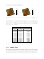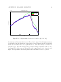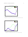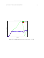
1
FEAP - - A Finite Element Analysis Program
Version 8.2 Parallel User Manual
Robert L. Taylor1 & Sanjay Govindjee1,2
1
Department of Civil and Environmental Engineering
University of California at Berkeley
Berkeley, California 94720-1710, USA
E-Mail: [email protected]
2
Center of Mechanics
ETH Zurich
CH-8092 Zurich
Switzerland
E-Mail: [email protected]
March 2008
Contents
1 Introduction
1.1 General features . . . . . . . . . . . . . . . . .
1.2 Problem solution . . . . . . . . . . . . . . . .
1.3 Graph partitioning . . . . . . . . . . . . . . .
1.3.1 METIS version . . . . . . . . . . . . .
1.3.2 ParMETIS: Parallel graph partitioning
1.3.3 Structure of parallel meshes . . . . . .
.
.
.
.
.
.
1
1
2
2
2
3
4
.
.
.
.
.
.
.
.
6
6
6
8
8
8
9
10
10
. . . . . . . . . . . . . . .
. . . . . . . . . . . . . . .
. . . . . . . . . . . . . . .
. . . . . . . . . . . . . . .
with global node numbers
. . . . . . . . . . . . . . .
. . . . . . . . . . . . . . .
. . . . . . . . . . . . . . .
. . . . . . . . . . . . . . .
. . . . . . . . . . . . . . .
. . . . . . . . . . . . . . .
11
12
12
13
13
14
15
15
16
17
17
18
2 Input files for parallel solution
2.1 Basic structure of parallel file . . . . . . . . .
2.1.1 DOMAIN - Domain description . . . .
2.1.2 BLOCked - Block size for equations . .
2.1.3 LOCal to GLOBal node numbering . .
2.1.4 GETData and SENDdata - Ghost node
2.1.5 MATRix storage – equation structure .
2.1.6 EQUAtion number data . . . . . . . .
2.1.7 END DOMAIN record . . . . . . . . .
3 Solution process
3.1 Command language statements . . . . . . .
3.1.1 PETSc Command . . . . . . . . . . .
3.2 Solution of linear equations . . . . . . . . .
3.2.1 Tolerance for equation solution . . .
3.2.2 GLIST & GNODE: Output of results
3.3 Eigenproblem solution for modal problems .
3.3.1 Subspace method solutions . . . . . .
3.3.2 Arnoldi/Lanczos method solutions .
3.4 Graphics output . . . . . . . . . . . . . . . .
3.4.1 GPLOt command . . . . . . . . . . .
3.4.2 NDATa command . . . . . . . . . . .
A Solution Command Manual
.
.
.
.
.
.
.
.
.
.
.
.
.
.
.
.
.
.
.
.
.
.
.
.
.
.
.
.
.
.
.
.
.
.
.
.
.
.
.
.
.
.
. . . . . . .
. . . . . . .
. . . . . . .
. . . . . . .
retrieve and
. . . . . . .
. . . . . . .
. . . . . . .
.
.
.
.
.
.
.
.
.
.
.
.
.
.
.
.
.
.
. . .
. . .
. . .
. . .
send
. . .
. . .
. . .
.
.
.
.
.
.
.
.
.
.
.
.
.
.
.
.
.
.
.
.
.
.
.
.
.
.
.
.
.
.
.
.
.
.
.
.
.
.
.
.
.
.
21
i
CONTENTS
ii
B Program structure
B.1 Introduction . . . . . . . . . . . . . . . . . . . . . . . . . . . . . . . . .
B.2 Building the parallel version . . . . . . . . . . . . . . . . . . . . . . . .
35
35
36
C Element modification features
37
D Added subprograms
39
E Parallel Validation
E.1 Timing Tests . . . . . . . . . . . . . . . . . . . .
E.1.1 Linear Elastic Block . . . . . . . . . . . .
E.1.2 Nonlinear Elastic Block . . . . . . . . . . .
E.1.3 Plasticity . . . . . . . . . . . . . . . . . .
E.1.4 Box Beam: Shells . . . . . . . . . . . . . .
E.1.5 Linear Elastic Block: 10-node Tets . . . .
E.1.6 Transient . . . . . . . . . . . . . . . . . .
E.1.7 Mock turbine . . . . . . . . . . . . . . . .
E.1.8 Mock turbine Small . . . . . . . . . . . . .
E.1.9 Mock turbine Tets . . . . . . . . . . . . .
E.1.10 Eigenmodes of Mock Turbine . . . . . . .
E.2 Serial to Parallel Verification . . . . . . . . . . . .
E.2.1 Linear elastic block . . . . . . . . . . . . .
E.2.2 Box Beam . . . . . . . . . . . . . . . . . .
E.2.3 Linear Elastic Block: Tets . . . . . . . . .
E.2.4 Mock Turbine: Modal Analysis . . . . . .
E.2.5 Transient . . . . . . . . . . . . . . . . . .
E.2.6 Nonlinear elastic block: Static analysis . .
E.2.7 Nonlinear elastic block: Dynamic analysis
E.2.8 Plastic plate . . . . . . . . . . . . . . . . .
E.2.9 Transient plastic . . . . . . . . . . . . . .
.
.
.
.
.
.
.
.
.
.
.
.
.
.
.
.
.
.
.
.
.
.
.
.
.
.
.
.
.
.
.
.
.
.
.
.
.
.
.
.
.
.
.
.
.
.
.
.
.
.
.
.
.
.
.
.
.
.
.
.
.
.
.
.
.
.
.
.
.
.
.
.
.
.
.
.
.
.
.
.
.
.
.
.
.
.
.
.
.
.
.
.
.
.
.
.
.
.
.
.
.
.
.
.
.
.
.
.
.
.
.
.
.
.
.
.
.
.
.
.
.
.
.
.
.
.
.
.
.
.
.
.
.
.
.
.
.
.
.
.
.
.
.
.
.
.
.
.
.
.
.
.
.
.
.
.
.
.
.
.
.
.
.
.
.
.
.
.
.
.
.
.
.
.
.
.
.
.
.
.
.
.
.
.
.
.
.
.
.
.
.
.
.
.
.
.
.
.
.
.
.
.
.
.
.
.
.
.
.
.
.
.
.
.
.
.
.
.
.
.
.
.
.
.
.
.
.
.
.
.
.
.
.
.
.
.
.
.
.
.
.
.
.
.
.
.
.
.
.
.
.
.
43
44
44
44
44
45
45
46
46
47
47
48
48
48
49
50
51
54
57
58
58
59
List of Figures
1.1
Structure of stiffness matrix in partitioned equations.
. . . . . . . . .
5
2.1
Input file structure for parallel solution.
. . . . . . . . . . . . . . . . .
7
E.1 Comparison of Serial (left) to Parallel (right) mode shape 1 degree of
freedom 1. . . . . . . . . . . . . . . . . . . . . . . . . . . . . . . . . . .
E.2 Comparison of Serial (left) to Parallel (right) mode shape 2 degree of
freedom 2. . . . . . . . . . . . . . . . . . . . . . . . . . . . . . . . . . .
E.3 Comparison of Serial (left) to Parallel (right) mode shape 3 degree of
freedom 3. . . . . . . . . . . . . . . . . . . . . . . . . . . . . . . . . . .
E.4 Comparison of Serial (left) to Parallel (right) mode shape 4 degree of
freedom 1. . . . . . . . . . . . . . . . . . . . . . . . . . . . . . . . . . .
E.5 Comparison of Serial (left) to Parallel (right) mode shape 5 degree of
freedom 2. . . . . . . . . . . . . . . . . . . . . . . . . . . . . . . . . . .
E.6 Comparison of Serial (left) to Parallel (right) mode shape 1 degree of
freedom 1. . . . . . . . . . . . . . . . . . . . . . . . . . . . . . . . . . .
E.7 Comparison of Serial (left) to Parallel (right) mode shape 2 degree of
freedom 2. . . . . . . . . . . . . . . . . . . . . . . . . . . . . . . . . . .
E.8 Comparison of Serial (left) to Parallel (right) mode shape 3 degree of
freedom 3. . . . . . . . . . . . . . . . . . . . . . . . . . . . . . . . . . .
E.9 Comparison of Serial (left) to Parallel (right) mode shape 4 degree of
freedom 1. . . . . . . . . . . . . . . . . . . . . . . . . . . . . . . . . . .
E.10 Comparison of Serial (left) to Parallel (right) mode shape 5 degree of
freedom 2. . . . . . . . . . . . . . . . . . . . . . . . . . . . . . . . . . .
E.11 von Mises stresses at the end of the loading. (left) serial, (right) parallel
E.12 Z-displacement for the node located at (0.6, 1.0, 1.0). . . . . . . . . .
E.13 11-component of the stress in the element nearest (1.6, 0.2, 0.8). . . . .
E.14 1st principal stress at the node located at (1.6, 0.2, 0.8). . . . . . . . .
E.15 von Mises stress at the node located at (1.6, 0.2, 0.8). . . . . . . . . . .
iii
52
52
52
53
53
54
54
55
55
55
59
60
61
61
62
Chapter 1
INTRODUCTION
1.1
General features
This manual describes features for the parallel version of the general purpose Finite
Element Analysis Program (FEAP). It is assumed that the reader of this manual is
familiar with the use of the serial version of FEAP as described in the basic user
manual.[1] It is also assumed that the reader of this manual is familiar with the finite
element method as describe in standard reference books on the subject (e.g., The Finite
Element Method, 6th edition, by O.C. Zienkiewicz, R.L. Taylor, et al. [2, 3, 4]).
The current version of the parallel code modifies the serial version of FEAP to interface to the PETSc library system available from Argonne National Laboratories.[5, 6]
In addition the METIS[7] and ParMETIS[8] libraries are used to partition each mesh
for parallel solution. The present parallel version of FEAP may only be used in a
UNIX/Linux environment and includes an integrated set of modules to perform:
1. Input of data describing a finite element model;
2. An interface to METIS[7] to perform a graph partitioning of the mesh nodes. A
stand alone module exists to also use ParMETIS[8] to perform the graph partitioning.;
3. An interface to PETSc[5, 6, 9] to perform the parallel solution steps;
4. Construction of solution algorithms to address a wide range of applications; and
5. Graphical and numerical output of solution results.
1
CHAPTER 1. INTRODUCTION
1.2
2
Problem solution
The solution of a problem using the parallel versions starts from a standard input
file for a serial solution. This file must contain all the data necessary to define nodal
coordinate, element connection, boundary condition codes, loading conditions, and
material property data. That is, if it were possible, this file must be capable of solving
the problem using the serial version. However, at this stage of problem solving the only
solution commands included in the file are those necessary to partition the problem for
the number of processors to be used in the parallel solution steps.
1.3
Graph partitioning
To use the parallel version of FEAP it is first necessary to construct a standard input
file for the serial version of FEAP. Preparation of this file is described in the FEAP
User Manual.[1]
1.3.1
METIS version
After the file is constructed and its validity checked, a one processor run of the parallel
program may be performed using the GRAPh solution command statement followed by
an OUTD solution command. To use this option a basic form for the input file is given
as:
FEAP * * Start record and title
...
Control and mesh description data
...
END mesh
BATCh
GRAPh node numd
OUTDomains <UNBLocked>
END batch
...
STOP
! METIS partitions ’numd’ nodal domains
! Creates ’numd’ meshes
where the node on the GRAPh command is optional. The meaning of the UNBLocked
option is explained below in Sect. 1.3.3 Using these commands, METIS [7] will split a
CHAPTER 1. INTRODUCTION
3
problem into numd partitions by nodes and output numd input files for a subsequent
parallel solution of the problem.
1.3.2
ParMETIS: Parallel graph partitioning
A stand alone parallel graph partitioner also exists. The parallel partitioner, partition
(located in the ./parfeap/partition subdirectory), uses ParMETIS [8] to perform the
construction of the nodal split. To use this program it is necessary to have a FEAP
input file that contains all the nodal coordinate and all the element connection records.
That is, there must be a file with the form:
FEAP * * Start record and title
Control record
COORdinates
All nodal coordinate records
...
ELEMent
All element connection records
...
remaining mesh statemnts
...
END mesh
The flat form for an input file may be created from any FEAP input file using the
solution command:
OUTM
This creates an input file with the same name and the extender ”.rev”. If a TIE
mesh manipulation command is used the output mesh will remove unused nodes and
renumber the node numbers.
Once the flat input file exists a parallel partitioning is performed by executing the
command
mpirun -np nump partition numd Ifile
where nump is the number of processors that ParMETIS uses, numd is the number of
mesh partitions to create and Ifile is the name of the flat FEAP input file. For an
input file originally named Ifilename, the program creates a graph file with the name
graph.filename. The graph file contains the following information:
CHAPTER 1. INTRODUCTION
4
1. The processor assignment for each node (numnp)
2. The pointer array for the nodal graph (numnp+1)
3. The adjacency lists for the nodal graph
To create the partitioned mesh input files the flat input file is executed again (in the
same directory containing the graph.filename) as a single processor run of the parallel
FEAP together with the solution commands
GRAPh FILE
OUTDomains <UNBLocked>
See the next section for the meaning of the option UNBLocked.
It is usually possible to also create the graph.file in parallel using the command set
OUTMesh
GRAPh PARTition numd
OUTDomains <UNBLocked>
where numd is the number of domains to create. In this case the parameter nump is
equal to numd.1 The use of the command OUTMesh is required to ensure that a flat
input file is available and after execution it is destroyed.
1.3.3
Structure of parallel meshes
It is assumed that numd represents the number of processors to be used in the parallel
solution. Each partition is assigned numpn nodes. The number can differ slightly among
the various partitions but is approximately the total number of nodes in the problem
divided by numd. In the current release, no weights are assigned to the nodes to reflect
possible differences in solution effort. It is next necessary to check which elements are
attached to each of these nodes. Once this is performed it is then necessary to check
each of the attached elements for any additional nodes that are not part of the current
nodal partition. These are called ghost nodes. The sum of the nodes in a partition
(numpn) and its ghost nodes defines the total number of nodes in the current partition
data file (i.e., the total number of nodes, numnp, in each mesh partition).
In the parallel solution the global equations are numbered sequentially from 1 to the
total number of equations in the problem (numteq). The nodes in partition 1 are
1
Use of this command set requires the path to the location of the partition program to be set in
the pstart.F file located in the parfeap directory.
CHAPTER 1. INTRODUCTION
5
associated with the first set of equations, the nodes in partition 2 the second set, etc.
For each partition, the stiffness and/or the mass matrix is also partitioned and each
partition matrix has two parts: (a) a diagonal block for all the nodes in the partition
(i.e., numpn nodes) and, (b) off diagonal blocks associated with the ghost nodes as
shown in Figure 1.1. In solving a set of linear equations
K du = R
associated with an implicit solution step, the solution vector du and the residual R
are also split according to each partition. The residual for each partition contains only
the terms associated with the equations of the partition. The solution vector, however,
must have both the terms associated with the partition as well as those associated with
the equations of its ghost nodes. If the equations are solved by an iterative method
using this form of partition it is only necessary to exchange values for the displacement
quantities associated with the respective ghost nodes.
There are two forms available to partition the equations: blocked and unblocked. By
default the equations are blocked and permit solution by PETSc’s preconditioned conjugate gradient method with either a Jacobi type preconditioner[5] or the Prometheus
multi-grid preconditioner[10] . If an unblocked form is requested (i.e., by an OUTMESH
UNBLocked command) only the Jacobi type preconditioner may be used.
In the next chapter we describe how the input data files for each partition are organized
to accomplish the partitioning just described.
K11
K1g
K2g
K22
K
3g
Processor 1
K2g
K
33
Processor 2
K
3g
Processor 3
Figure 1.1: Structure of stiffness matrix in partitioned equations.
Chapter 2
Input files for parallel solution
After using the METIS or the ParMETIS partitioning algorithm on the total problem
(for example, that given by say the mesh file Ifilename) FEAP produces numd files
for the partitions and these serve as input for the parallel solution. Each new input
file is named Ifilename 0001, etc. up to the number of partitions specified (i.e., numd
partitions).
The first part of each file contains a standard FEAP input file for the nodes and
elements belonging to the partition. This is followed by a set of commands that begin
with DOMAin and end with END DOMAIN. All of the data contained between the DOMAin
and END DOMAIN is produced automatically by FEAP.
The file structure for a parallel solution is shown in Figure 2.1 and is provided only to
describe how the necessary data is given to each partition. No changes are allowed to
be made to these statements.
2.1
Basic structure of parallel file
Each part of the data following the END MESH statement performs a specific task in the
parallel solution. It is important that the data not be altered in any way as this can
adversely affect the solution process. Below we describe the role each data set plays
during the solution.
2.1.1
DOMAIN - Domain description
The DOMAIN data defines the number of nodes belonging to this partition (numpn), the
number of total nodes in the problem (numtn) and the number of total equations in the
6
CHAPTER 2. INPUT FILES FOR PARALLEL SOLUTION
FEAP * * Start record and title
...
Control and mesh description data for a partition
...
END MESH
DOMAin
numpn
numtn
numteq
<BLOCked> equations: Block size = ndf
LOCAl to GLOBal node numbers
...
GETData POINter
...
nget_pnt
GETData VALUes
...
nget_val
SENDdata POINter
...
nsend_pnt
SENDdata VALUes
...
nsend_val
MATRix storage
...
<EQUAtion> numbers (If BLOCked not used)
...
END DOMAIN
INCLude solve.filename
STOP
Figure 2.1: Input file structure for parallel solution.
7
CHAPTER 2. INPUT FILES FOR PARALLEL SOLUTION
8
problem (numteq). Note that the number of nodes in the partition (numpn) is always
less or equal to the number of nodes given on the control record (numnp) due to the
presence of the ghost nodes. The sum over all partitions of the number of nodes in
each partition (numpn) is equal to the total number of nodes in the problem (numtn).
2.1.2
BLOCked - Block size for equations
This data set is optional. If a blocked form for the equations is requested (this is
the default) this data set defines the block size. The block size is always equal to the
number of degrees of freedom specified on the control record (i.e., ndf) and the blocked
form of the equations is grouped into small blocks of size ndf.
2.1.3
LOCal to GLOBal node numbering
Each record in this set defines three values: (1) a local node number in the partition;
(2) the global node associated with the local number; and (3) the global equation block
number associated with the local node. The first numpn records in the set are the nodes
associated with the current partition the remaining records with the ghost nodes.
2.1.4
GETData and SENDdata - Ghost node retrieve and
send
The current partition retrieves (GETData) the solution values for its ghost nodes from
other partitions. The data is divided into two parts: (1) A POINTER part which tells
the number of values to obtain from each partition and (2) The VALUes list of local
node numbers needing values. The pointer data is given as
GETData POINter nparts
np_1
np_2
...
np_nparts
where np i defines the number in partition-i (note the number should be a zero for the
current partition record). The nodal values list is given as
GETData VALUes nvalue
local_node_1
CHAPTER 2. INPUT FILES FOR PARALLEL SOLUTION
9
local_node_2
...
local_node_nvalue
The local node i numbers are grouped so that the first np 1 are obtained from processor 1, the next np 2 from processor 2, etc. The local node 1 is the number of a
local ghost node to be obtained from another processor and may appear only once in
the list of GETData VALUes.
A corresponding pair of lists is given for the data to be sent (SENDdata) to the other
processors. The lists have identical structure to the GETData lists and are given by
SENDdata POINter nparts
np_1
np_2
...
np_nparts
and
SENDdata VALUes nvalue
local_node_1
local_node_2
...
local_node_nvalue
where again the local node i numbers are grouped so that the first np 1 are sent to
processor 1, the next np 2 to processor 2, etc. It is possible for a local node number
to appear more than once in the SENDdata VALUes list as it could be a ghost node for
more than one other partition.
2.1.5
MATRix storage – equation structure
Each equation in the global matrix consists of the number of terms that are associated
with the current partition and the number of terms associated with other partitions.
This information is provided for each equation (equation block) by the MATRix storage
data set. Each record in the set is given by the global equation number followed by
the number of terms associated with the current partition and then the number of
terms associated with other partitions. The use of this data is critical to obtain rapid
assembly of the global matrices by PETSc. If it is incorrect the assembly time will be
very large compared to the time needed to compute the matrix coefficients.
CHAPTER 2. INPUT FILES FOR PARALLEL SOLUTION
10
When the equations are blocked the data is given for each block number. In the blocked
form every node has ndf equations. Thus, the first ndf equations are associated with
block 1, the second with block 2, etc. The total number of equations numteq for this
form is numtn × ndf. Each record of the MATRix storage data is given by the global
block number, the number of blocks associated with the current partition and the
number of blocks associated with other partitions. For any node in which all degree-offreedoms (DOF) are of displacement type the number of blocks in the current partition
will be 1 and the number in other blocks will be zero. That is, the equations for any
node in which all DOF’s are fixed will be given as:
I dua = Ra = dū
where dū denotes a specified valued for the solution.
2.1.6
EQUAtion number data
This data set is not present when the equations are blocked. However, when the equations are unblocked it is necessary to fully describe the equation numbering associated
with each node in the partition. This is provided by the EQUAtion number data set.
The set consists of numnp records which contain the local node number followed by
the global equation number for every degree-of-freedom associated with the node. If a
degree-of-freedom is restrained (i.e., of displacement type) the equation is not active
and a zero appears. This form results in fewer unknown values but may not be used
with any equation solution requiring a blocked form (in particular, Prometheus).
2.1.7
END DOMAIN record
The parallel data is terminated by the END DOMAIN record. It is followed by the solution
commands.
Chapter 3
Solution process
Once the parallel input mesh files are created an execution of the parallel version of
feap may be performed using the command line statement
-@${MPIEXEC} -s all -np $(NPROC) $(FEAPRUN) -ksp_type cg -pc_type jacobi
or
-@${MPIEXEC} -s all -np $(NPROC) $(FEAPRUN) -ksp_type cg -pc_type prometheus
(for details on other required and optional parameters see the makefile in the parfeap
subdirectory). The parameters setting the number of processors (NPROC) and the execution path FEAPRUN must be defined before issuing the command.
Once FEAP starts the input file should be set to Ifilename 0001 where filename is
the name of the solution file to be solved. Each processor reads its input file up to the
END MESH statement and then starts processing command language statements.
In a parallel solution using FEAP the same command language statements must be
provided for each partition. This is accomplished using the statement
INCLude solve.filename
where filename is the name of the input data file with the leading I and the trailing
partition number removed. Thus for the file named Iblock 0001 the command is given
as solve.block. All solution commands are then placed in a file with this name and
can include both BATCh and INTEractive commands. For example a simple solution
may be given by the commands
11
CHAPTER 3. SOLUTION PROCESS
12
BATCh
PETSc ON
TOL ITER 1.d-07 1.d-08 1.d+20
TANGent,,1
END
INTEractive
placed in the solve.filename file. Note hat both batch and interactive modes of solution are optionally included. Interactive commands need only be entered once and are
sent to other processors automatically if in the makefile for initiating the execution
of the parallel FEAP the target parameter -s all appears. In the subsequent subsections we describe some of the special commands that control the parallel execution
mode of FEAP
3.1
Command language statements
Most of the standard command language statements available in the serial version of
FEAP (see users manual [1]) may be used in the parallel version of feap. New commands are available also that are specifically related to performing a parallel solution.
3.1.1
PETSc Command
The PETSc command is used to activate the parallel solution process. The command
PETSc <ON,OFF>
may be used to turn on and off the parallel execution It is only required for single
processor solutions and is optional when two or more processors are used in the solution
process. When required, it should always be the first solution command.
The command may also be used with the VIEW parameter to create outputs for the
tangent matrix, solution residual or mass matrix. Thus, use as
PETSc VIEW
MASS
PETSc NOVIew
will create a file named mass.m that contains all the non-zero values of the total mass
matrix. The parameter VIEW turns on output arrays and this remains in effect for all
CHAPTER 3. SOLUTION PROCESS
13
commands until the command is given with the NOVIew parameter. The file is created
in a format that may be directly used by MATLAB.[11] This command should only be
used with small problems to verify the correctness of results as large files will result
otherwise.
3.2
Solution of linear equations
The parallel version of FEAP can use all of the SLES (linear solvers) available in PETSc
as well as the parallel multigrid solver, Prometheus[10] . The actual type of linear solver
used is specified in the makefile located in the parfeap directory (see, Sect. 3 above).
Once the solution is initiated the solution of linear equations is performed whenever a
TANG,,1 or SOLVe command is given.
The types of solvers and the associated preconditioners tested to date are described in
Table 3.1.
Solver
CG
CG
MINRES
MINRES
GMRES
GMRES
GMRES
GMRES
Preconditioner
Jacobi
Prometheus
Jacobi
Prometheus
Jacobi
Prometheus
Block Jacobi
ASM(ILU)
Notes
Generally requires fewest iterations
Often gives indefinite factor.
Table 3.1: Linear solvers and preconditioners tested.
The solvers, together with the necessary options for preconditioning may be specified
in the Makefile as parameters to the mpiexec command. Two examples of possible
options are contained in the Makefile.
3.2.1
Tolerance for equation solution
The basic form of solution for linear equations is currently restricted to a preconditioned
conjugate gradient (PCG) method. Two basic solution forms are defined in the makefile
contained in the parfeap subdirectory. The first (feaprun) uses the solver contained in
the PETSc library and the second is Prometheus (feaprun-mg) available from Columbia
University.[10] In general the performance of Prometheus is much better than the first
form.
CHAPTER 3. SOLUTION PROCESS
14
Termination tolerances for the solvers are given by either
TOL ITER rtol atol dtol
or
ITER TOL rtol atol dtol
where rtol is the tolerance for the preconditioned equations, atol the tolerance for
the original equations and dtol a value at which divergence is assumed. The default
values are:
rtol = 1.d − 8 ;
atol = 1.d − 16 and dtol = 1.d + 16
For many problems it is advisable to check that the actual solution is accurate since
termination of the equation solution is performed based on the rtol value. A check
should be performed using the command sequence
TANG,,1
LOOP,,1
FORM
SOLV
NEXT
since the TANG command has significant set up costs, especially for Prometheus. Indeed,
for some problems more than one iteration is needed in the loop.
3.2.2
GLIST & GNODE: Output of results with global node
numbers
In normal execution each partition creates its own output file (e.g., Ofilename 0001,
etc.) with printed data given with the local node and element numbers of the processor’s input data file. In some cases the global node numbers are known and it is desired
to identify which processor to which the node is associated. This may be accomplished
by including a GLISt command in the solution statements along with the list of global
node numbers to be output. The option is restricted to 3 lists, each with a maximum
of 100 nodes. The command sequence is given by:
BATCh
GLISt,,<1,2,3>
CHAPTER 3. SOLUTION PROCESS
15
END
list of global node numbers, 8 per record
! blank termination record
The list will be converted by each processor into the local node numbers to be output
using the command
DISP LIST <1,2,3>
The command may also be used with VELOcity, ACCEleration, and STREss. See
manual pages in the FEAP Users Manual.[1]
It is also possible to directly output the global node number associated with individual
local node numbers using the command statement
DISP GNODe nstart nend ninc
where nstart and nend are global node numbers. This command form also may be
used with VELOcity, ACCEleration, and STREss.
3.3
Eigenproblem solution for modal problems
The computation of the natural modes and frequencies of free vibration of an undamped
linear structural problem requires the solution of the general linear eigenproblem
KΦ = MΦΛ
In the above K and M are the stiffness and mass matrices, respectively, and Φ and Λ
are the normal modes and frequencies squared. Normally, the constraint
ΦT M Φ = I
is used to scale the eigenvectors. In this case one also obtains the relation
ΦT K Φ = Λ
3.3.1
Subspace method solutions
The subspace algorithm contained in FEAP has been extended to solve the above
problem in a parallel mode. The use of the subspace algorithm requires a linear solution
of the equations
Kx = y
CHAPTER 3. SOLUTION PROCESS
16
for each vector in the subspace and for each subspace iteration. The parallel subspace
solution is performed using the command set
TANGent
MASS <LUMPed,CONSistent>
PSUBspace <print> nmodes <nadded>
where nmodes is the desired number of modes, nadded is the number of extra vectors
used to accelerate the convergence (default if maximum of nmodes and 8) and print
produces a print of the subspace projections of K and M. The accuracy of the computed eigenvalues is the maximum of 1.d − 12 and the value set by the TOL solution
command. The method may be used with either a lumped or a consistend mass matrix.
If it is desired to extract 10 eigenvectors with 8 added vectors and 20 iterations are
needed to converge to an acceptable error it is necessary to perform 360 solutions of the
linear equations. Thus, for large problems the method will be very time consuming.
3.3.2
Arnoldi/Lanczos method solutions
In order to reduce the computational effort the Arnoldi/Lanczos methods implemented
in the ARPACK module available from Rice University[12] has been modified to work
with the parallel version of FEAP.
Two modes of the ARPACK solution methods are included in the program:
1. Mode 1: Solves the problem reformed as
M−1/2 K M−1/2 Ψ = Ψ Λ
where
Φ = M−1/2 Ψ
This form is most efficient when the mass matrix is diagonal (lumped) and, thus,
in the current release of parallel FEAP is implemented only for diagonal (lumped)
mass forms. This mode form is specified by the solution command set
TANGent
MASS LUMPed
PARPack LUMPed
nmodes <maxiters> <eigtol>
where nmodes is the number of desired modes. Optionally, maxiters is the
number of iterations to perform (default is 300) and eigtol the solution tolerance
on eigenvalues (default is the maximum of 1.d − 12 and the values set by the
command TOL.
CHAPTER 3. SOLUTION PROCESS
17
2. Mode 3: Solves the general linear eigenproblem directly and requires solution of
the linear problem
Kx = y
for each iteration. Fewer iterations are normally required than in the subspace
method, however, the method is generally far less efficient than the Mode 1 form
described above. This form is given by the set of commands
TANGent
MASS <LUMPed,CONSistent>
PARPack <SYMMetric> nmodes <maxiters> <eigtol>
Use of the command MASS alone also will employ a consistent mass (or the mass
produced by the quadrature specified).
3.4
Graphics output
During a solution the graphics commands may be given in a standard manner. However,
each processor will open a graphics window and display only the parts that belong to
that processor. Scaling is also done processor by processor unless the PLOT RANGe
command is used to set the range of a set of plot values.
3.4.1
GPLOt command
An option does exist to collect all the results together and present on a single graphics
window. This option also permits postscript outputs to be constructed and saved in
files. To collect the results together it is necessary to write the results to disk for each
item to be graphically presented. This is accomplished using the GPLOt command.
This command has the options
GPLOt DISPlacement n
GPLOt STREss
n
GPLOt PSTRess
n
where n denotes the component of a displacement (DISP), nodal stress (STRE) or principal stress (PSTRE). Each use of the command creates a file on each processor with the
form
Gproblem_domain.xyyyy
CHAPTER 3. SOLUTION PROCESS
18
where problem domain is the name of the problem file for the domain; x is d, s or p
for a displacement, stress or principal stress, respectively; and yyyy is a unique plot
number (it will be between 0001 and 9999).
3.4.2
NDATa command
Once the GPLOt files have been created they may be plotted using a serial execution of
the parallel FEAP program (i.e., using the Iproblem file. The command may be given
in INTEractive mode only as one of the options:
Plot > NDATa DISPl
n
Plot > NDATa STREss n
Plot > NDATa PSTRess n
where n is the value of yyyy used to write the file.
WARNING: Plots by FEAP use substantial memory and thus this option may not
work for very large problems. One should minimize the number of commands used
during input of the problem description (i.e., remove input commands in the mesh
that create new memory).
Bibliography
[1] R.L. Taylor. FEAP - A Finite Element Analysis Program, User Manual. University of California, Berkeley. http://www.ce.berkeley.edu/˜rlt.
[2] O.C. Zienkiewicz, R.L. Taylor, and J.Z. Zhu. The Finite Element Method: Its
Basis and Fundamentals. Elsevier, Oxford, 6th edition, 2005.
[3] O.C. Zienkiewicz and R.L. Taylor. The Finite Element Method for Solid and
Structural Mechanics. Elsevier, Oxford, 6th edition, 2005.
[4] O.C. Zienkiewicz, R.L. Taylor, and P. Nithiarasu. The Finite Element Method for
Fluid Dynamics. Elsevier, Oxford, 6th edition, 2005.
[5] S. Balay, K. Buschelman, W.D. Gropp, D. Kaushik, M.G. Knepley,
L.C. McInnes, B.F. Smith, and H. Zhang.
PETSc Web page, 2001.
http://www.mcs.anl.gov/petsc.
[6] S. Balay, K. Buschelman, V. Eijkhout, W.D. Gropp, D. Kaushik, M.G. Knepley,
L.C. McInnes, B.F. Smith, and H. Zhang. PETSc users manual. Technical Report
ANL-95/11 - Revision 2.1.5, Argonne National Laboratory, 2004.
[7] G. Karypis. METIS: Family of multilevel partitioning algorithms. http://wwwusers.ce.umn.edu/˜karypis/metis/.
[8] G. Karypis.
ParMETIS parallel graph partitioning, 2003.
users.cs.unm.edu/˜karypis/metis/parmetis/).
http://www-
[9] S. Balay, W.D. Gropp, L.C. McInnes, and B.F. Smith. Efficient management
of parallelism in object oriented numerical software libraries. In E. Arge, A. M.
Bruaset, and H. P. Langtangen, editors, Modern Software Tools in Scientific Computing, pages 163–202. Birkhäuser Press, 1997.
[10] M. Adams. PROMETHEUS: Parallel multigrid solver library for unstructured
finite element problems. http://www.columbia.edu/˜ma2325.
[11] MATLAB. www.mathworks.com, 2003.
19
BIBLIOGRAPHY
20
[12] R. Lehoucq, K. Maschhoff, D. Sorensen, and C. Yang. ARPACK: Arnoldi/lanczos
package for eigensolutions. http://www.caam.rice.edu/software/ARPACK/.
[13] R.L. Taylor. FEAP - A Finite Element Analysis Program, Installation Manual.
University of California, Berkeley. http://www.ce.berkeley.edu/˜rlt.
Appendix A
Solution Command Manual Pages
FEAP has a few options that are used only to solve parallel problems. The commands
are additions to the command language approach in which users write each step using
available commands. The following pages summarize the commands currently added
to the parallel version of FEAP.
21
APPENDIX A. SOLUTION COMMAND MANUAL
DISPlacements
22
FEAP COMMAND INPUT COMMAND MANUAL
disp,gnod,<n1,n2,n3>
Other options of this command are described in the FEAP User Manual. The command DISPlacement may be used to print the current values of the solution generalized
displacement vector associated with the global node numbers of the original mesh. The
command is given as
disp,gnod,n1,n2,n3
prints out the current solution vector for global nodes n1 to n2 at increments of n3
(default increment = 1). If n2 is not specified only the value of node n1 is output. If
both n1 and n2 are not specified only the first node solution is reported.
APPENDIX A. SOLUTION COMMAND MANUAL
GLISt
23
FEAP COMMAND INPUT COMMAND MANUAL
glist,,n1
<values>
The command GLISt is used to specify lists of global node numbers for output of
nodal values. It is possible to specify up to three different lists where the list number
corresponds to n1 (default = 1). The list of nodes to be output is input with up to
8 values per record. The input terminates when less than 8 values are specified or a
blank record is encountered. No more than 100 items may be placed in any one list.
List outputs are then obtained by specifying the command:
name,list,n1
where name may be DISPlacement,VELOcity,ACCEleration, or STREss and n1 is the desired
list number.
Example:
BATCh
GLISt,,1
END
1,5,8,20
BATCh
DISP,LIST,1
...
END
The global list of nodes is processed to determine the processor and the associated
local node number. Each processor then outputs its active values (if any) and gives
both the local node number in the partition as well as the global node number.
APPENDIX A. SOLUTION COMMAND MANUAL
GPLOt
gplo
gplo
gplo
gplo
24
FEAP COMMAND INPUT COMMAND MANUAL
disp
velo
acce
stre
n
n
n
n
Use of plot commands during execution of the parallel version of FEAP create the same
number of graphic windows as processors used to solve the problem. Each window
contains only the part of the problem contained on that processor.
The use of the GPLOt command is used to save files containing the results for all nodal
dispacements, velocities, accelerations or stresses in the total problem. The only action
occuring after the use of this command is the creation of a file containing the current
results for the quantity specified. Repeated use of the command creates files with
different names.
These results may be processed by a single processor run of the problem using the
mesh for the total problem. To display the nodal values command NDATa is used. See
manual page on NDATa.
APPENDIX A. SOLUTION COMMAND MANUAL
GRAPh
25
FEAP COMMAND INPUT COMMAND MANUAL
grap,,num d
grap node num d
grap file
grap part num d
The use of the GRAPh command activates the interface to the METIS multilevel partioner. The partition into num d parts is performed based on a nodal graph. The nodal
partition divides the total number of nodes (i.e., numnp values) into num d nearly equal
parts.
If the GRAPh command is given with the option file the partition data is input from the
file graph.filename where filename is the same as the input file without the leading
I character. The data contained in the graph.filename is created using the stand
alone partitioner program which employs the PARMETIS multilevel partitioner.
It is also possible to execute PARMETIS to perform the partitioning directly during
a mesh input. It is necessary to have a mesh which contains all the nodal coordinate
and element data in the input file. This is accomplished using the command set
OUTMesh
GRAPh PARTition num_d
OUTDomain meshes
where num d is the number of domains to create. The command OUTMesh creates a
file with all the nodal and element data and is destroyed after execution of the GRAPh
command.
APPENDIX A. SOLUTION COMMAND MANUAL
ITERative
26
FEAP COMMAND INPUT COMMAND MANUAL
iter,,,icgit
iter,bpcg,v1,icgit
iter,ppcg,v1,icgit
iter,tol,v1,v2,v3
The ITERative command sets the mode of solution to iterative for the linear algebraic
equations generated by a TANGent. Currently, iterative options exist only for symmetric,
positive definite tangent arrays, consequently the use of the UTANgent command should
be avoided. An iterative solution requires the sparse matrix form of the tangent matrix
to fit within the available memory of the computer.
Serial solutions
In the serial version the solution of the equations is governed by the relative residual for
the problem (i.e., the ratio of the current residual to the first iteration in the current
time step). The tolerance for convergence may be set using the ITER,TOL,v1,v2 option.
The parameter v1 controls the relative residual error given by
1/2
(RT R)i
1/2
≤ v1 (RT R)0
and, for implementations using PETSc the parameter v2 controls the absolute residual
error given by
1/2
(RT R)i ≤ v2
The default for v1 is 1.0d-08 and for v2 is 1.0d-16. By default the maximum number
of iterations allowed is equal to the number of equations to be solved, however, this
may be reduced or increased by specifying a positive value of the paramter icgit.
The symmetric equations are solved by a preconditioned conjugate gradient method.
Without options, the preconditioner is taken as the diagonal of the tangent matrix.
Options exist to use the diagonal nodal blocks (i.e., the ndf × ndf nodal blocks, or
reduced size blocks if displacement boundary conditions are imposed) as the preconditioner. This option is used if the command is given as ITERative,BPCG. Another option
is to use a banded preconditioner where the non-zero profile inside a specified half band
is used. This option is used if the command is given as ITERative,PPCG,v1, where v1 is
the size of the half band to use for the preconditioner.
The iterative solution options currently available are not very effective for poorly conditioned problems. Poor conditioning occurs when the material model is highly non-
APPENDIX A. SOLUTION COMMAND MANUAL
27
linear (e.g., plasticity); the model has a long thin structure (like a beam); or when
structural elements such as frame, plate, or shell elements are employed. For compact
three dimensional bodies with linear elastic material behavior the iterative solution is
often very effective.
Another option is to solve the equations using a direct method (see, the DIREct command language manual page).
Parallel solutions
For the parallel version the control of the PETSc preconditioned iterative solvers is
controlled by the command
ITER TOL itol atol dtol
where itol is the tolerance for the preconditioned equations (default 1.d − 08), atol
is the tolerance for the original equations (default 1.d − 16) and dtol is a divergence
protection when the equations do not converge (default 1.d + 16).
APPENDIX A. SOLUTION COMMAND MANUAL
NDATa
28
FEAP COMMAND INPUT COMMAND MANUAL
ndat
ndat
ndat
ndat
disp
velo
acce
stre
n
n
n
n
This command is used in a single processor execution using the mesh for the total
problem. It is necessary for files to be created during a parallel execution using the
GPLOt command (See manual page on GPLOt).
The command is given by
NDATa DISPlacement num
where the parameter num is the number corresponding to the order the DISPlacement
are created. Thus, the command sequence
NDATa DISPlacement 2
NDATa STREss
2
would display the results for the second files created for the displacements and stresses.
APPENDIX A. SOLUTION COMMAND MANUAL
OUTDomain
29
FEAP COMMAND INPUT COMMAND MANUAL
outd,,<bsize>
outd bloc <bsize>
outd unbl
The use of the OUTDomain command may only be used after the GRAPh command
partitions the mesh into num d parts (see GRAPh command language page for details).
Using the command OUTDomain or OUTDomain BLOCked creates num d input files for a
subsequent parallel solution in which the coefficient arrays will be created in a blocked
form. The parameter bsize defines the block size and must be an integer divisor of
ndf. That is if ndf = 6 then bsize may be 1, 2, 3, or 6. By default each block in
the equations has a size ndf. The setting of the block size can significantly reduce the
amount of storage needed to store the sparse coefficient matrix created by TANGent or
UTANgent when a problem has a mix of element types. For example if a problem has
a large number of solid elements with 3 degrees of freedom per node and additional
frame or shell elements with 6 degrees of freedom per node, specifying bsize = 3 can
save considerable memory.
APPENDIX A. SOLUTION COMMAND MANUAL
PETSc
pets
pets
pets
pets
pets
30
FEAP COMMAND INPUT COMMAND MANUAL
on
off
view
noview
The use of the PETSc command turns on or off to activate or deactivate parallel
solution options, respectively. To turn on parallel computing the command may be
given in the simple form: PETSc. When more than one partition is created, i.e., the
number of solution processors is 2 or more, the PETSc option is on by default. The
command must be the first command of the command language program when only 1
processor is used.
The option PETSc VIEW will result in a file for all the non-zero coefficients in the tangent
matrix to be output into a file. The output is in a MATLAB format. This option should
only be used for very small problems to check that a formulation produces correct
results (i.e., there is another set of terms to which a comparison is to be made). The
option is turned off using the statement PETSc NOVIew. The default is NOVIew.
APPENDIX A. SOLUTION COMMAND MANUAL
STREss
31
FEAP COMMAND INPUT COMMAND MANUAL
stre.gnod,<n1,n2,n3>
Other options for this command are given in the FEAP User Manual. The STREss
command is used to output nodal stress results at global node numbers n1 to n2 at
increments of n2 (default = 1).
The command specified as:
stre,gnode,n1,n2,n3
If n3 is not given an increment of 1 is used. If n2 is not given only values for node n1
are output. If n1 is not specified the values at global node 1 are output.
APPENDIX A. SOLUTION COMMAND MANUAL
TOLerance
32
FEAP COMMAND INPUT COMMAND MANUAL
tol,,v1
tol,ener,v1
tol,emax,v1
tol,iter,v1,v2,v3
The TOL command is used to specify the solution tolerance values to be used at various
stages in the analysis. Uses include:
1. Convergence of nonlinear problems in terms of the norm of energy in the current
iterate (the inner, dot, product of the displacement increment and the solution
residual vectors).
2. Convergence of iterative solution of linear equations.
3. Convergence of the subspace eigenpair solution which is measured in terms of the
change in subsequent eigenvalues computed.
The basic command, TOL,,tol, without any arguments sets the parameter tol used in
the solution of non-linear problems where the command sequence
LOOP,,30
TANG,,1
NEXT
is given. In this case, the loop is terminated either when the number of iterations
reaches 30 (or whatever number is given in this position) or when the energy error is
less than tol. The energy error is given by
Ei = (duT R)i ≤ tol (duT R)0 = E0
in which R is the residual of the equatons and du is the solution increment. The default
value of tol for the solution of nonlinear problems is 1.0d-16.
The TOL command also permits setting a value for the energy below which convergence
is assumed to occur. The command is issued as TOL,ENERgy,v1 where v1 is the value of
the converged energy (i.e., it is equivalent to the tolerance times the maximum energy
value). Normally, FEAP performs nonlinear iterations until the value of the energy
is less than the TOLerance value times the value of the energy from the first iteration
APPENDIX A. SOLUTION COMMAND MANUAL
33
as shown above. However, for some transient problems the value of the initial energy
is approaching zero (e.g., for highly damped solutions which are converging to some
steady state limit). In this case, it is useful to specify the energy for convergence
relative to early time steps in the solution. Convergence will be assumed if either the
normal convergence criteria or the one relative to the specified maximum energy is
satisfied.
The TOL command also permits setting the maximum energy value used for convergence. The command is issued as
TOL,EMAX}imum,v1
where v1 is the value of the maximum energy quantity. Note that the TIME command
sets the maximum energy to zero, thus, the value of EMAXimum must be reset after
each time step using, for example, a set of commands:
LOOP,time,n
TIME
TOL,EMAX,5.e+3
LOOP,newton,m
TANG,,1
NEXT
etc.
NEXT
to force convergence check against a specified maximum energy. The above two forms
for setting the convergence are nearly equivalent; however, the ENERgy tolerance form
can be set once whereas the EMAXimum form must be reset after each time command.
The command
TOL ITERation itol atol dtol
is used to control the solution accuracy when an iterative solution process is used to
solve the equations
K du = R
In this case the parameter itol sets the relative error for the solution accuracy, i.e.,
when
1/2
1/2
(RT R)i ≤ itol (RT R)0
The parameter atol is only used when solutions are performed using the KSP schemes
in a PETSc implementation to control the absolute residual error
1/2
(RT R)i
≤ atol
APPENDIX A. SOLUTION COMMAND MANUAL
34
The dtol parameter is used to terminate the solution when divergence occurs. The
default for itol is 1.0d-08, that for atol is 1.0d-16 and for dtol is 1.0d+16.
Appendix B
Program structure
B.1
Introduction
This section describes the parallel infrastructure for the general purpose finite element
program, FEAP.[1] The current version of the parallel code modifies the serial version
of FEAP to interface to the PETSc library system available from Argonne National
Laboratories.[5, 6] In addition the METIS[7] and ParMETIS[8] libraries are used to partition each mesh for parallel solution.
The necessary modifications and additions for the parallel features are contained in the
directory parfeap. There are five sub-directories contained in parfeap:
1. arpack: Contains the subprograms and include files needed for the ARPACK
eigen solution module (see Section 3.3).
2. blas: Contains Fortran versions of the BLAS routines used by FEAP. It is
recommended that when ever possible a BLAS library be used. These routines
are provided only for cases where no library is available.
3. lapack: Contains the subprograms from LAPACK used in the parallel version.
4. partition: Contains the program and include file used to construct the partition
graph using ParMETIS (see Section 1.3).
5. windows: Contains the replacement for subprogram p metis.f for use in a Windows version of the program.1
1
N.B. No testing of any parallel solutions other than mesh partitioning using a serial version of
FEAP has been attempted to date.
35
APPENDIX B. PROGRAM STRUCTURE
B.2
36
Building the parallel version
In order to build a parallel version of FEAP it is necessary first to install and compile
a serial version (see instructions in the FEAP Installation manual.[13] ). Once a serial
version is available and tested the routines for arpack should be compiled. To compile
change the directory to
ver82/packages/arpack/archive
Compile using the command
make install
This wilil build an archive named arpacklib.a that will be linked with the program
later. Next change the directory to
ver82/parfeap/packages/arpack
and again compile using the command
make install
This will build an archive named parpacklib.a that will also be linked with the parallel
code later. Finally, change the directory to
ver82/parfeap
and compile the parallel version using the command
make install
This will create a parallel version feap in the parfeap directory. If any subprogram is
missing it may be necessary to compile routines contained in directories
ver82/packages/lapack
ver82/packages/blas
Then modify the makefile in the parfeap directory to include the new archives and
recompile the program using
make install
If any errors still exist, ensure that all definitions contained in the makefile have been
properly set using setenv and/or that PETSc has been properly installed.
Appendix C
Element modification features
The use of the eigensolver with the LUMPed option requires all elements to form a valid
diagonal (lumped) mass matrix. One option to obtain a lumped mass is the use of a
quadrature formula that samples only at nodes.[2] In this case all element that use C0
interpolation forms have mass coefficients computed from
Z
X
Mab =
Na ρ Nb dV ≈
Na (ξl ) ρ Nb (ξl ) j(ξl ) Wl
Ωe
l
where ξl and Wl are the quadrature points and j(ξl ) the Jacobian of the coordinate
transformation. For C0 interpolations the shape functions have the property[2]
1 ;a = b
Na (ξb ) = δab =
0 ; a 6= b
Thus if ξl = ξb (the nodal points) and Wl > 0 the mass matrix produced will be
diagonal and positive definite.
For quadrilateral and brick elements of linear order use of product forms of trapezoidal
rule sample at all nodes and satisfy the above criterion. Similarly use of Simpson’s
rule for quadratic order quadrilaterals or bricks also satisfies the above rule. Similarly,
for triangular and tetrahedral elements of linear order nodal integrations has positive
weights and produces a valid diagonal mass. However, for a 6-node quadratic order
triangle or a 10-node quadratic order tetrahedron no such formula exists. Indeed, the
nodal quadrature formula for these elements samples only at the mid-edge nodes and
has zero weights Wb at the vertex nodes. Such a formula is clearly not valid for use
in computing a diagonal mass matrix. The problem can be cured however by merely
adding an addition node at the baricenter of the triangle or tetrahedron and thus
producing a 7-node or 11-node element, respectively. Another advantage exists in that
these elements may also be developed as mixed models that permit solution of problems
in which the material behavior is nearly incompressible (e.g., see references [2] and [3]).
37
APPENDIX C. ELEMENT MODIFICATION FEATURES
38
FEAP has been modified to include use of 7-node triangular and 11-node tetrahedral elements. Furthermore, nodal quadrature formulas have been added and may be
activated for each material by including the quadrature descriptor
QUADrature NODAl
or, alternatively, for the whole problem as
GLOBal
QUADrature NODAl
! Other global options or blank record to terminate
Existing meshes of 10-node tetrahedral elements may be converted using the user function umacr0.f included in the subdirectory parfeap. A similar function to convert
6-node triangular element may be easily added using this function as a model.
The solution of problems composed of quadratic order tetrahedral elements can be
difficulty when elements have very bad aspect ratios or have large departures from
straight edges. A more efficient solution is usually possible using linear order elements.
Two options are available to convert 10-node tetrahedral elements to 4-node tetrahedral
ones. These are available as user functions in subdirectory parfeap. The first option
converts each 10-node element to a single 4-node element. This leads to a problem with
many fewer nodes and, thus, is generally quite easy to solve compared to the original
problem. This option is given in subprogram umacr8.f. A second option keeps the
same number of nodes and divides each 10-node element into eight (8) 4-node elements.
This option is given in subprogram umacr9.f.
One final option exists o modify meshes with 10-node elements. In this option all
curved sides are made straight and mid-edge nodes are placed at the center of each
edge. This option is given in subprogram umacr6.f.
Appendix D
Added subprograms
The tables below describe the modifications and extensions to create the current parallel
version. Table D.1 describe modifications made to subroutines contained in the serial
version. Table D.2 presents the list of subprograms added to create the mesh for each
individual processor and to permit basic parallel solution steps. Table D.3 presents the
list of subprograms modified for subspace eigensolution and those added to interface
to the ARPACK Arnoldi/Lanczos eigensolution methods. Finally, Table D.4 describes
the list of user functions that may be introduced to permit various additional solution
steps with the parallel or serial version.
39
APPENDIX D. ADDED SUBPROGRAMS
Filename
filnam.F
fppsop.F
gamma1.f
palloc.f
pbases.F
pcontr.f
pdelfl.f
pextnd.f
pform.f
plstop.F
pmacio.F
pmacr.f
pmacr1.f
pmacr3.f
pmodal.f
pmodin.F
pplotf.F
premas.f
prtdis.f
40
Description of actions performed
Set up file names for input/output
Output postscript file from each processor
Compute energy for line search
Allocate memory for arrays
Parallel application of multiple base excitations for modal solutions
Main driver for FEAP
Delete all temporary files at end of execution
Dummy subprogram for external node determination
Parallel driver to compute element arrays and assemble global arrays
Closes open plot windows, deletes arrays and stops execution
Controls input of solution commands
Solution command driver: Adds call to pmacr7 for parallel options
Solution command driver 1
Solution command driver 3
Parallel modal solution of linear transient problems
Input initial conditions for modal solutions
Driver for plot commands
Initialize data for mass computation
Output nodal displacement values for real solutions: Includes global
node numbers for parallel runs
prtstr.f Output nodal stress values: Includes global node numbers for parallel
runs
pstart.F Set starting values and control names of data files for each processor
scalev.F Parallel scale of vector to have maximum element of +1.0
Table D.1: Subprograms modified for parallel solutions.
APPENDIX D. ADDED SUBPROGRAMS
Filename
adomnam.f
bserchi.f
p metis.f
pcompress.f
pddot.f
pdgetv0.f
pdnrm2.f
pdomain.F
petscmi.F
petscsr.F
pmacr7.F
pminvsqr.F
pmodify.f
pparlo.f
prwext.F
psetb.F
smodify.f
41
Description of actions performed
Set file extender for processor number
Use binary search to find a specified node number
METIS driver to compute partition graph
Compute compressed form of element array
Parallel dot product
Generates random vector for ARPACK and forces residual to be in
range of operator
Parallel Euclidean norm of a vector
Input of domain data for parallel solutions
Sends and receives maximum value of data
Sends and receives real data values
Solution command driver 7: Parallel features added
Modify element arrays for effects of non-zero specified displacements
Parallel set of assembly information for element arrays
Add extender to parallel data files
Transfer PETSC vector to local arrays
Modify blocked element tangent for imposed displacements
Table D.2: New subprograms added for parallel solutions.
Filename
arfeaps.f
aropk.f
aropm.f
parfeaps.F
parkv.F
parmv.F
paropk.F
paropm.F
pdsaitr.f
pdsaup2.f
pdsaupd.f
pdseupd.f
psubsp.F
psproja.f
psprojb.F
Description of actions performed
Serial ARPACK driver for symmetric eigenproblems
Serial main operator for ARPACK Mode 1 and Mode 3 eigensolution
Serial mass operator for ARPACK eigensolution
Parallel ARPACK driver for symmetric eigenproblems
Parallel ARPACK routine to compute product of stiffness times vector
Parallel ARPACK routine to compute product of mass times vector
Parallel ARPACK application of stiffness operator
Parallel ARPACK application of mass operator
Parallel ARPACK reverse communication interface for ARPACK
Parallel ARPACK intermediate level interface called by pdsaupd
Parallel ARPACK reverse communication interface for implicitly
restarted Arnoldi Iteration
Parallel ARPACK computation of converged eigenvalues and vectors
Parallel subspace eigenpair driver
Parallel subspace projection of stiffness matrix
Parallel subspace projection of mass matrix
Table D.3: Added or modified subprograms for eigenpair extraction.
APPENDIX D. ADDED SUBPROGRAMS
Filename
uasble.F
uasblem.F
umacr4.f
umacr5.f
umacr6.f
umacr7.f
umacr8.f
umacr9.f
umacr0.f
upc.F
upremas.F
usolve.F
42
Description of actions performed
Parallel assembly of element stiffness arrays into PETSc matrices
Parallel assembly of element mass arrays into PETSc matrices
Parallel ARPACK interface for PETSc instructions
Serial ARPACK interface for PETSc instructions
Average coordinate locations for mid-edge nodes on quadratic order
elements
Convert 10-node tetrahedral elements into 11-node tetrahedra
Convert mesh of 10-node tetrahedral elements into mesh of 4-node
tetrahedra
Convert mesh of 10-node tetrahedral elements into mesh of 4-node
tetrahedral elements
Convert mesh of 10-node tetrahedral elements into mesh of 11-node
tetrahedral elements
Sets up user defined preconditioners (PC) for PETSc solutions
Parallel interface to initialize mass assembly into PETSc arrays
Parallel solver interface for PETSc linear solutions
Table D.4: Modified and new user subprograms.
Appendix E
Parallel Validation
The validation of the parallel portion of FEAP has been performed on a number of
different basic problems to verify that the parallel extension of FEAP will solve such
problems and that the parallel version performs properly in the sense that it scales
with processor number in an acceptable manner. Furthermore, a series of comparison
tests have been performed to verify that the parallel version of the program produces
the same answers as the serial version. Because of the enormous variety of analyses
that one can perform with FEAP, it is not possible to provide parallel tests for all
possible combinations of program features. Nonetheless, below one will find some
basic validation tests that highlight the performance of the parallel version of the code
on a variety of problems.
All validation tests were performed on a cluster of AMD Opteron 250 processors,
connected together via a Quadrics QsNet II interconnect. Code performance is often
strongly related to the computational sub-systems employed. All tests reported utilized
GCC v3.3.4, MPI v1.2.4, PETSc v2.3.2-p3, AMD ACML (BLAS/LAPACK) v3.5.0,
c
ParMetis v3.1, Prometheus v1.8.5, and ARPACK 2001.
The batch scheduler assures
that no other jobs are running on the same compute nodes during the runs. All runs
have utilized the algebraic multigrid solver Prometheus in blocked form with coordinate
information. Run times are as reported from PETSc summary statistics from a single
run; Mflops are those associated with PETSc’s KSPsolve object; Number of solves is
the total number of Ax = b solves during the KSP iterations in the total problem, and
Scaling % of ideal is computed as (Mflopsnp /np)/(Mflops2 /2) × 100.
43
APPENDIX E. PARALLEL VALIDATION
E.1
E.1.1
44
Timing Tests
Linear Elastic Block
In this test a linear elastic unit block discretized into 70×70×70 8-node brick elements
is clamped on one face and loaded on the opposite face with a uniform load in all
coordinate directions. In blocked form there are 1,073,733 equations in this problem.
Number
Processors
2
4
8
16
32
E.1.2
Time (sec)
129.20
71.69
35.77
21.30
13.19
Mflops
Number
Scaling
(KSP Solve)
Solves % Ideal
1241
13
2171
13
87
4646
14
94
8347
14
84
14561
14
73
Nonlinear Elastic Block
In this test a nonlinear neohookean unit block discretized into 50 × 50 × 50 8-node
brick elements is clamped on one face and loaded on the opposite face with a uniform
load in all coordinate directions. In blocked form there are 397,953 equations in this
problem. To solve the problem, to default tolerances, takes 4 Newton iterations within
which there are on average 12 KSP iterations.
Number
Processors
2
4
8
16
32
E.1.3
Time (sec)
166.7
82.66
43.48
27.15
15.58
Mflops
Number Scaling
(KSP Solve)
Solves % Ideal
1142
53
2356
54
103
4642
53
102
7846
56
86
13988
52
77
Plasticity
In this test one-quarter of a plate with a hole is modeled using 364500 8-node brick
elements and pulled in tension beyond yield. The problem involves 10 uniform size load
steps which drives the plate well into the plastic range; each load step takes between
3 and 10 Newton iterations. There are 1,183,728 equations. Due to the large number
APPENDIX E. PARALLEL VALIDATION
45
of overall KSP iterations needed for this problem, it has only been solved using 8, 16,
and 32 processors. Scaling is thus computed relative to the 8 processor run.
Number
Processors
2
4
8
16
32
E.1.4
Time (sec)
220.80
107.70
59.03
Mflops
Number Scaling
(KSP Solve)
Solves % Ideal
4434
2973
8425
2908
95
15645
2868
88
Box Beam: Shells
In this test a box beam is modeled using 40000 linear elastic 4-node shell elements (6dof per node). The beam has a 1 to 1 aspect ratio with each face modeled by 100 × 100
elements. One end is fully clamped and the other is loaded with equal forces in the
three coordinate directions. There are 242,400 equations; the block size is 6 × 6.
Number
Processors
2
4
8
16
32
E.1.5
Time (sec)
49.43
16.37
12.46
5.03
3.28
Mflops
Number Scaling
(KSP Solve)
Solves % Ideal
510
195
1619
190
159
1972
188
97
5246
181
129
8177
184
100
Linear Elastic Block: 10-node Tets
In this test the linear elastic unit block from the first test is re-discretized using 10-node
tetrahedral elements. As in the 8-node brick case, there are 1,073,733 equations in this
problem. In the table below, we also provide the ratio of times for the “same” problem when solved using 8-node brick elements. This indicates the difficulty in solving
problems (iteratively) that emanate from quadratic approximations. Essentially, per
dof, tets solve in the ideal case 1.5 times slower.
APPENDIX E. PARALLEL VALIDATION
Number
Processors
2
4
8
16
32
E.1.6
Time (sec)
216.8
110.4
56.62
31.44
17.07
46
Mflops
Number Scaling Slow down
(KSP Solve)
Solves % Ideal
vs. Brick
1299
30
1.7
2615
30
101
1.5
5059
29
97
1.6
9370
30
90
1.5
17659
28
85
1.3
Transient
In this test a short (2 to 1 aspect ratio) neohookean beam is subjected to a step
displacement in the axial direction. The modeling employs symmetry boundary conditions on three orthogonal planes. The beam is discretized into uniform size 8-node
brick elements 10 × 10 × 20 for a total of 7623 equations. The dynamic vibrations of
the material are followed for 40 time steps using Newmark’s method. The steep drop
off in performance should be noted. This is due to the small problems size. There is
too little work for each processor to be effectively utilized here.
Number
Processors
2
4
8
16
32
E.1.7
Time (sec)
95.37
58.91
39.03
32.15
33.61
Mflops
Number Scaling
(KSP Solve)
Solves % Ideal
1079
1385
1687
1420
78
2645
1382
61
3138
1376
36
3123
1371
18
Mock turbine
In this test we model a mock turbine fan blade with 12 fins. The system is loaded using
an Rω 2 body force term which is computed consistently. Overall there are 1,080,000
8-node brick elements in the mesh and 3,415,320 equations. It should be noted that
problem, at roughly 3.5 million equations, provides enough work for the processors that
even at 32 processors there is no degradation of performance. The scaling is perfect.
APPENDIX E. PARALLEL VALIDATION
Number
Processors
2
4
8
16
32
E.1.8
Time (sec)
854.3
362.4
172.9
88.99
46.68
47
Mflops
Number Scaling
(KSP Solve)
Solves % Ideal
806
116
1931
112
120
4085
110
127
8232
115
128
16159
112
125
Mock turbine Small
In this test we model again a mock turbine fan blade with 12 fins. The system is loaded
using an Rω 2 body force term which is computed consistently. Overall, however, there
are only 552960 8-node brick elements in the mesh and 1,771,488 equations.
Number
Processors
2
4
8
16
32
E.1.9
Time (sec)
347.40
199.50
91.63
47.68
26.32
Mflops
Number Scaling
(KSP Solve)
Solves % Ideal
1097
125
1878
132
86
4064
122
93
8024
126
91
15400
119
88
Mock turbine Tets
In this test we model again a mock turbine fan blade with 12 fins. The system is loaded
using an Rω 2 body force term which is computed consistently. This time however we
utilize 10-node tetrahedral elements with a model that has 1,771,488 equations. This
computation can be directly compared to the small mock turbine benchmark. The
slow down is given in the last column of the table below.
Number
Processors
2
4
8
16
32
Time (sec)
507.7
304.2
131.0
70.01
41.83
Mflops
Number Scaling Slow Down
(KSP Solve)
Solves % Ideal
vs. Brick
1193
126
1.5
1934
129
81
1.5
4675
131
98
1.4
8860
134
93
1.5
16238
127
85
1.6
APPENDIX E. PARALLEL VALIDATION
E.1.10
48
Eigenmodes of Mock Turbine
In this test we look at the computation of the first 5 eigen modes of the small (552960
element) mock turbine model. Again, the mesh is composed of 8-node brick elements
and the model has 1,771,488 equations. A lumped mass is utilized and the algorithm
tested is the ARPA symmetric option. Due to the large number of inner-outer iterations
the timing runs are done only for 8, 16, and 32 processors. Scaling is thus computed
relative to the 8 processor run.
Number
Processors
2
4
8
16
32
E.2
Time (sec)
916.9
507.1
248.3
Mflops
Number Scaling
(KSP Solve)
Solves % Ideal
3757
2744
7122
2876
95
14042
2723
93
Serial to Parallel Verification
Serial to parallel code verification is reported upon below. For all test run, the program
is run in serial mode (with a direct solver) and in parallel mode on 4 processors (forcing
inter- and intra-node communications). Then various computation output quantities
are compared between the parallel and serial runs. In all cases, it is observed that the
outputs match to the computed accuracy.
E.2.1
Linear elastic block
In this test a linear elastic unit block discretized into 5 × 5 × 5 8-node brick elements
is clamped on one face and loaded on the opposite face with a uniform load in all
coordinate directions. The displacements are compared at global nodes 100 and 200
and the maximum overall principal stress is also determined from both runs. All values
are seen to be identical. For the parallel runs, the processor number containing the
value is given in parenthesis and the reported node number is the local processor node
number.
Node
100
200
Serial Displacements
x-coor
y-coor
z-coor
x-disp
y-disp
z-disp
6.00E-01 8.00E-01 4.00E-01 -1.3778E-01 1.1198E+00 1.1241E+00
2.00E-01 6.00E-01 1.00E+00 -4.1519E-01 2.3568E-01 2.6592E-01
APPENDIX E. PARALLEL VALIDATION
49
Serial Max Principal Stress
Node
Stress
1
4.0881E+02
(P)Node
(4)49
(2)38
Parallel Displacements
x-coor
y-coor
z-coor
x-disp
y-disp
z-disp
6.00E-01 8.00E-01 4.00E-01 -1.3778E-01 1.1198E+00 1.1241E+00
2.00E-01 6.00E-01 1.00E+00 -4.1519E-01 2.3568E-01 2.6592E-01
Parallel Max Principal Stress
(P)Node
Stress
(3)1
4.0881E+02
Note: Processor 3’s local node 1 corresponds to global node 1.
E.2.2
Box Beam
In this test a linear elastic unit box-beam discretized into 4 × 20 × 20 4-node shell
elements is clamped on one face and loaded on the opposite face with a uniform load
in all coordinate directions. The displacements are compared at global nodes 500 and
1000 and the maximum overall principal bending moment is also determined from both
runs. All values are seen to be identical. For the parallel runs, the processor number
containing the value is given in parenthesis and the reported node number is the local
processor node number.
Node
500
1000
Serial Displacements/Rotations
x-coor
y-coor
z-coor
x-disp
y-disp
z-disp
x-rot
y-rot
z-rot
8.00E-01 1.00E-01 1.00E+00 3.6632E-03 -3.2924E-03 2.3266E-03
4.4272E-02 -7.3033E-04 -2.1595E-02
1.00E+00 3.00E-01 2.00E-01 2.2972E-02 1.5303E-03 1.6876E-02
4.8140E-02 2.8224E-02 -1.3278E-01
Serial Max Principal
Bending Moment
Node
Stress
1
1.7091E+01
APPENDIX E. PARALLEL VALIDATION
(P)Node
(1)29
(2)280
50
Parallel Displacements/Rotations
x-coor
y-coor
z-coor
x-disp
y-disp
z-disp
x-rot
y-rot
z-rot
8.00E-01 1.00E-01 1.00E+00 3.6632E-03 -3.2924E-03 2.3266E-03
4.4272E-02 -7.3033E-04 -2.1595E-02
1.00E+00 3.00E-01 2.00E-01 2.2972E-02 1.5303E-03 1.6876E-02
4.8140E-02 2.8224E-02 -1.3278E-01
Parallel Max Principal
Bending Moment
(P)Node
Stress
(4)1 1.7091E+01
Note: Processor 4’s local node 1 corresponds to global node 1.
E.2.3
Linear Elastic Block: Tets
In this test a linear elastic unit block discretized into 162 10-node tetrahedral elements
is clamped on one face and loaded on the opposite face with a uniform load in all
coordinate directions. The displacements are compared at global nodes 55 and 160
and the maximum overall principal stress is also determined from both runs. All
values are seen to be identical. For the parallel runs, the processor number containing
the value is given in parenthesis and the reported node number is the local processor
node number.
Node
55
160
Serial Displacements
x-coor
y-coor
z-coor
x-disp
y-disp
z-disp
8.33E-01 0.00E+00 1.67E-01 4.9509E-01 4.3175E-01 4.2867E-01
8.33E-01 1.67E-01 5.00E-01 2.1305E-01 4.2030E-01 4.1548E-01
Serial Max
Principal Stress
Node
Stress
8 9.0048E+01
(P)Node
(3)23
(1)17
Parallel Displacements
x-coor
y-coor
z-coor
x-disp
y-disp
z-disp
8.33E-01 0.00E+00 1.67E-01 4.9509E-01 4.3175E-01 4.2867E-01
8.33E-01 1.67E-01 5.00E-01 2.1305E-01 4.2030E-01 4.1548E-01
APPENDIX E. PARALLEL VALIDATION
51
Parallel Max
Principal Stress
(P)Node
Stress
(4)6 9.0048E+01
Note: Processor 4’s local node 6 corresponds to global node 8.
E.2.4
Mock Turbine: Modal Analysis
In this test we examine a small mock turbine model with 30528 equations, where the
discretization is made with 8-node brick elements. We compute using the serial code
(subspace method) the first 5 eigenvalues using a lumped mass. With the parallel
code, we compute the same eigenvalues using a parallel eigensolve (implicitly restarted
Arnoldi). The computed frequencies and from the first 5 modes are compared and seen
to be the same within the accuracy of the computation.
Serial Eigenvalues (rad/sec)2
Mode 1
Mode 2
Mode 3
Mode 4
Mode 5
8.10609997E-02 8.13523152E-02 8.13523152E-02 9.33393875E-02 9.33393875E-02
Parallel Eigenvalues (rad/sec)2
8.10609790E-02 8.13522933E-02 8.13522972E-02 9.33393392E-02 9.33393864E-02
The comparison of eigenvectors is a bit harder for this problem because of repeated
eigenvalues. The first eigenvalue is not repeated and it can easily be seen that the serial and parallel codes have produced the same eigenmode (up to an arbitrary scaling
factor). Eigenvalues 2 and 3 are repeated and thus the vectors computed are, permissibly, drawn from a subspace and thus direct comparison is not evident. The same
holds for eigenvalues 4 and 5; though, it can be observed that vector 4 from the serial
computation does closely resemble vector 5 from the parallel computations – i.e. they
appear to be drawn from a similar region of the subspace.
As a test of the claim of differing eigenmodes due to selection of different eigenvectors
from a subspace, we also compute the first 5 modes of an asymmetric structure that
does not possess repeated eigenvalues. The basic geometry is that of perturbed cube.
The first 5 eigenvalues and modes are compared and show proper agreement to within
the accuracy of the computations for both the eigenvalues and the eigenmodes.
APPENDIX E. PARALLEL VALIDATION
_________________
DISPLACEMENT 1
-7.23E-02
-6.02E-02
-4.82E-02
-3.61E-02
-2.41E-02
-1.20E-02
8.68E-14
1.20E-02
2.41E-02
3.61E-02
4.82E-02
6.02E-02
7.23E-02
Value = 4.53E-02 Hz.
52
_________________
EIGENV
1
-3.45E-04
-2.88E-04
-2.30E-04
-1.73E-04
-1.15E-04
-5.75E-05
9.00E-12
5.75E-05
1.15E-04
1.73E-04
2.30E-04
2.88E-04
3.45E-04
Time = 0.00E+00
Figure E.1: Comparison of Serial (left) to Parallel (right) mode shape 1 degree of
freedom 1.
_________________
DISPLACEMENT 2
-7.07E-02
-5.89E-02
-4.72E-02
-3.54E-02
-2.36E-02
-1.18E-02
-4.54E-05
1.17E-02
2.35E-02
3.53E-02
4.71E-02
5.88E-02
7.06E-02
Value = 4.54E-02 Hz.
_________________
EIGENV
2
-3.04E-04
-2.54E-04
-2.03E-04
-1.52E-04
-1.01E-04
-5.07E-05
6.36E-08
5.08E-05
1.02E-04
1.52E-04
2.03E-04
2.54E-04
3.04E-04
Time = 0.00E+00
Figure E.2: Comparison of Serial (left) to Parallel (right) mode shape 2 degree of
freedom 2.
_________________
DISPLACEMENT 3
-1.00E+00
-8.33E-01
-6.67E-01
-5.00E-01
-3.33E-01
-1.67E-01
3.91E-10
1.67E-01
3.33E-01
5.00E-01
6.67E-01
8.33E-01
1.00E+00
Value = 4.54E-02 Hz.
_________________
EIGENV
3
-6.77E-03
-5.64E-03
-4.51E-03
-3.38E-03
-2.26E-03
-1.13E-03
4.33E-08
1.13E-03
2.26E-03
3.39E-03
4.51E-03
5.64E-03
6.77E-03
Time = 0.00E+00
Figure E.3: Comparison of Serial (left) to Parallel (right) mode shape 3 degree of
freedom 3.
APPENDIX E. PARALLEL VALIDATION
_________________
DISPLACEMENT 1
-5.53E-02
-4.61E-02
-3.69E-02
-2.77E-02
-1.84E-02
-9.22E-03
-5.87E-12
9.22E-03
1.84E-02
2.77E-02
3.69E-02
4.61E-02
5.53E-02
Value = 4.86E-02 Hz.
53
_________________
EIGENV
4
-4.94E-04
-4.12E-04
-3.30E-04
-2.47E-04
-1.65E-04
-8.24E-05
4.72E-10
8.24E-05
1.65E-04
2.47E-04
3.30E-04
4.12E-04
4.94E-04
Time = 0.00E+00
Figure E.4: Comparison of Serial (left) to Parallel (right) mode shape 4 degree of
freedom 1.
_________________
DISPLACEMENT 2
-6.98E-02
-5.82E-02
-4.65E-02
-3.49E-02
-2.33E-02
-1.16E-02
5.23E-12
1.16E-02
2.33E-02
3.49E-02
4.65E-02
5.82E-02
6.98E-02
Value = 4.86E-02 Hz.
_________________
EIGENV
5
-3.70E-04
-3.08E-04
-2.47E-04
-1.85E-04
-1.23E-04
-6.17E-05
-8.57E-09
6.17E-05
1.23E-04
1.85E-04
2.47E-04
3.08E-04
3.70E-04
Time = 0.00E+00
Figure E.5: Comparison of Serial (left) to Parallel (right) mode shape 5 degree of
freedom 2.
APPENDIX E. PARALLEL VALIDATION
_________________
DISPLACEMENT 1
-5.42E-01
-4.46E-01
-3.50E-01
-2.54E-01
-1.58E-01
-6.15E-02
3.47E-02
1.31E-01
2.27E-01
3.23E-01
4.20E-01
5.16E-01
6.12E-01
Value = 1.06E+00 Hz.
54
_________________
EIGENV
1
-8.82E-01
-7.26E-01
-5.69E-01
-4.13E-01
-2.56E-01
-1.00E-01
5.65E-02
2.13E-01
3.69E-01
5.26E-01
6.82E-01
8.39E-01
9.95E-01
Time = 0.00E+00
Figure E.6: Comparison of Serial (left) to Parallel (right) mode shape 1 degree of
freedom 1.
_________________
DISPLACEMENT 2
-4.59E-01
-4.21E-01
-3.83E-01
-3.45E-01
-3.06E-01
-2.68E-01
-2.30E-01
-1.91E-01
-1.53E-01
-1.15E-01
-7.66E-02
-3.83E-02
0.00E+00
Value = 1.07E+00 Hz.
_________________
EIGENV
2
-1.67E-09
6.18E-02
1.24E-01
1.85E-01
2.47E-01
3.09E-01
3.71E-01
4.32E-01
4.94E-01
5.56E-01
6.18E-01
6.80E-01
7.41E-01
Time = 0.00E+00
Figure E.7: Comparison of Serial (left) to Parallel (right) mode shape 2 degree of
freedom 2.
Serial Eigenvalues (rad/sec)2
Mode 1
Mode 2
Mode 3
Mode 4
Mode 5
4.46503673E+01 4.52047021E+01 9.08496135E+01 2.32244552E+02 3.04152767E+02
Parallel Eigenvalues (rad/sec)2
4.46503674E+01 4.52047021E+01 9.08496136E+01 2.32244552E+02 3.04152767E+02
E.2.5
Transient
This test involves a mixed element test with shells, bricks, and beams under a random
dynamic load. The basic geometry consists of a cantilever shell with a brick block above
it which has an embedded beam protruding from it. The loading is randomly prescribed
on the top of the structure and the time histories are followed and compared for the
displacements at a particular point, the first stress component in a given element, and
the 1st principal stress and von Mises stress at a particular node. The time history is
followed for 20 time steps. The time integration is performed using Newmark’s method.
Agreement is seen to be perfect to the accuracy of the computations.
APPENDIX E. PARALLEL VALIDATION
_________________
DISPLACEMENT 3
-1.00E+00
-8.36E-01
-6.71E-01
-5.07E-01
-3.43E-01
-1.78E-01
-1.38E-02
1.51E-01
3.15E-01
4.79E-01
6.44E-01
8.08E-01
9.72E-01
Value = 1.52E+00 Hz.
55
_________________
EIGENV
3
-1.71E+00
-1.42E+00
-1.13E+00
-8.43E-01
-5.54E-01
-2.65E-01
2.42E-02
3.13E-01
6.02E-01
8.91E-01
1.18E+00
1.47E+00
1.76E+00
Time = 0.00E+00
Figure E.8: Comparison of Serial (left) to Parallel (right) mode shape 3 degree of
freedom 3.
_________________
DISPLACEMENT 1
0.00E+00
8.33E-02
1.67E-01
2.50E-01
3.33E-01
4.17E-01
5.00E-01
5.83E-01
6.67E-01
7.50E-01
8.33E-01
9.17E-01
1.00E+00
Value = 2.43E+00 Hz.
_________________
EIGENV
4
-5.18E-09
1.34E-01
2.69E-01
4.03E-01
5.38E-01
6.72E-01
8.06E-01
9.41E-01
1.08E+00
1.21E+00
1.34E+00
1.48E+00
1.61E+00
Time = 0.00E+00
Figure E.9: Comparison of Serial (left) to Parallel (right) mode shape 4 degree of
freedom 1.
_________________
DISPLACEMENT 2
-3.11E-01
-2.54E-01
-1.98E-01
-1.42E-01
-8.53E-02
-2.89E-02
2.75E-02
8.38E-02
1.40E-01
1.97E-01
2.53E-01
3.09E-01
3.66E-01
Value = 2.78E+00 Hz.
_________________
EIGENV
5
-1.07E+00
-9.01E-01
-7.37E-01
-5.73E-01
-4.08E-01
-2.44E-01
-8.00E-02
8.43E-02
2.49E-01
4.13E-01
5.77E-01
7.41E-01
9.06E-01
Time = 0.00E+00
Figure E.10: Comparison of Serial (left) to Parallel (right) mode shape 5 degree of
freedom 2.
APPENDIX E. PARALLEL VALIDATION
Time
0.0000E+00
2.5000E-01
5.0000E-01
7.5000E-01
1.0000E+00
1.2500E+00
1.5000E+00
1.7500E+00
2.0000E+00
2.2500E+00
2.5000E+00
2.7500E+00
3.0000E+00
3.2500E+00
3.5000E+00
3.7500E+00
4.0000E+00
4.2500E+00
4.5000E+00
4.7500E+00
5.0000E+00
z-Displacement at (0.6,1,1)
Serial Value Parallel Value
0.0000E+00
0.0000E+00
2.5181E-04
2.5181E-04
6.0174E-04
6.0174E-04
8.3328E-04
8.3328E-04
1.1250E-03
1.1250E-03
4.2010E-04
4.2010E-04
-7.1610E-04
-7.1610E-04
-1.3485E-03
-1.3485E-03
-2.2463E-03
-2.2463E-03
-1.8943E-03
-1.8943E-03
-9.1891E-04
-9.1891E-04
-6.8862E-04
-6.8862E-04
3.8305E-05
3.8306E-05
7.4499E-05
7.4499E-05
-1.4893E-04
-1.4893E-04
1.9767E-04
1.9767E-04
-1.8873E-04
-1.8873E-04
5.7747E-04
5.7747E-04
1.3268E-03
1.3268E-03
1.3859E-03
1.3859E-03
2.5241E-03
2.5241E-03
56
σxx in Element 1
Serial Value Parallel Value
0.0000E+00
0.0000E+00
3.9640E-02
3.9640E-02
1.3681E-01
1.3681E-01
1.9837E-01
1.9837E-01
2.2532E-01
2.2532E-01
1.5061E-01
1.5061E-01
-1.5312E-01
-1.5312E-01
-3.7978E-01
-3.7978E-01
-4.2376E-01
-4.2376E-01
-4.4457E-01
-4.4457E-01
-2.9013E-01
-2.9013E-01
-1.4539E-02
-1.4539E-02
1.1134E-03
1.1139E-03
-1.1587E-01
-1.1587E-01
1.1732E-01
1.1732E-01
4.3679E-02
4.3678E-02
-2.1461E-01
-2.1461E-01
2.6870E-01
2.6871E-01
3.2132E-01
3.2132E-01
1.3378E-01
1.3378E-01
6.6854E-01
6.6854E-01
APPENDIX E. PARALLEL VALIDATION
Time
Step
1
2
3
4
5
6
7
8
9
10
11
12
13
14
15
16
17
18
19
20
E.2.6
Stresses at Global Node 1
Serial Values
Parallel
I1 Principal
von Mises I1 Principal
7.5561E-02 9.5922E-02
7.5561E-02
2.4364E-01 3.0328E-01
2.4364E-01
3.4447E-01 4.2623E-01
3.4447E-01
4.0833E-01 5.1265E-01
4.0833E-01
2.5260E-01 3.1018E-01
2.5260E-01
1.5934E-01 3.6208E-01
1.5934E-01
3.5077E-01 7.7659E-01
3.5077E-01
4.3971E-01 9.8767E-01
4.3971E-01
4.4131E-01 9.8761E-01
4.4131E-01
2.5587E-01 5.6437E-01
2.5587E-01
1.2681E-01 2.3667E-01
1.2681E-01
2.3099E-02 3.6287E-02
2.3099E-02
9.8640E-02 2.2004E-01
9.8640E-02
2.0000E-01 2.4597E-01
2.0000E-01
1.1798E-01 1.6039E-01
1.1798E-01
1.8668E-01 4.2255E-01
1.8668E-01
4.3432E-01 5.2267E-01
4.3432E-01
5.8732E-01 7.3503E-01
5.8732E-01
2.7197E-01 3.7066E-01
2.7197E-01
1.1706E+00 1.4434E+00 1.1706E+00
57
Values
von Mises
9.5922E-02
3.0328E-01
4.2623E-01
5.1265E-01
3.1018E-01
3.6208E-01
7.7659E-01
9.8767E-01
9.8761E-01
5.6437E-01
2.3667E-01
3.6286E-02
2.2004E-01
2.4597E-01
1.6039E-01
4.2255E-01
5.2267E-01
7.3503E-01
3.7066E-01
1.4434E+00
Nonlinear elastic block: Static analysis
In this test a unit neo-hookean block is clamped on one side and subjected to surface
load on the opposite side. The displacements at two random nodes are compared as
well as the max equivalent shear stress (von Mises) over the entire mesh. All values
are seen to be the same between the serial and parallel computation.
Node
50
100
Serial Displacements
x-coor
y-coor
z-coor
x-disp
y-disp
z-disp
0.00E+00 0.00E+00 1.67E-01 0.0000E+00 0.0000E+00 0.0000E+00
1.67E-01 0.00E+00 3.33E-01
5.6861E-04 1.0501E-04 1.5672E-04
Serial Maximum
Equivalent Shear
0.881
APPENDIX E. PARALLEL VALIDATION
(P)Node
(2) 27
(2) 54
58
Parallel Displacements
x-coor
y-coor
z-coor
x-disp
y-disp
z-disp
0.00E+00 0.00E+00 1.67E-01 5.8777E-17 4.9956E-18 -6.3059E-17
1.67E-01 0.00E+00 3.33E-01 5.6861E-04 1.0501E-04 1.5672E-04
Note: Processor 2’s nodes 27 and 54 correspond to global nodes 50 and 100.
Parallel Maximum
Equivalent Shear
0.881
E.2.7
Nonlinear elastic block: Dynamic analysis
In this test a non-linear neo-hookean block is subjected to a step displacement at one
end while the other is end is clamped. The time history of the displacement at the
center of the block is followed. The time integration is performed using Newmark’s
method. Agreement is seen to be perfect to the accuracy of the computation.
Time
0.0000E+00
1.0000E-02
2.0000E-02
3.0000E-02
4.0000E-02
5.0000E-02
6.0000E-02
7.0000E-02
8.0000E-02
9.0000E-02
1.0000E-01
x-Displacement
Serial Run
Parallel Run
(Node 172)
(Node 25, Processor 3)
0.0000E+00
0.0000E+00
-6.6173E-07
-6.6173E-07
1.1588E-05
1.1588E-05
-4.8502E-05
-4.8502E-05
-4.8177E-05
-4.8177E-05
2.6189E-04
2.6189E-04
7.8251E-04
7.8251E-04
1.0785E-03
1.0785E-03
9.7015E-04
9.7015E-04
7.7567E-04
7.7567E-04
8.2252E-04
8.2252E-04
Note: Local node 25 of processor 3 corresponds to global node 172.
E.2.8
Plastic plate
In this test a small version of the quarter plastic plate from the timing runs is used with
4500 8-node brick elements. The problem involves 10 uniform size load steps which
APPENDIX E. PARALLEL VALIDATION
_________________
Mises Stress
59
_________________
PSTRESS
6
5.53E+01
5.53E+01
8.82E+01
1.21E+02
8.82E+01
1.21E+02
1.54E+02
1.54E+02
1.87E+02
2.20E+02
1.87E+02
2.20E+02
2.53E+02
2.53E+02
2.86E+02
3.18E+02
2.86E+02
3.18E+02
3.51E+02
3.51E+02
3.84E+02
4.17E+02
3.84E+02
4.17E+02
4.50E+02
4.50E+02
Time = 1.00E+00
Time = 1.00E+00
Figure E.11: von Mises stresses at the end of the loading. (left) serial, (right) parallel
drives the plate well into the plastic range. The displacement history is followed for a
point on the loaded edge of the plate. As seen in the tables the parallel and serial runs
match. Also shown are the contours of the von Mises stresses at the end of the run
with the plastic zone emanating from the plate hole; these also match perfectly within
the accuracy of the computation.
Load
Step
0.0000E+00
1.0000E-01
2.0000E-01
3.0000E-01
4.0000E-01
5.0000E-01
6.0000E-01
7.0000E-01
8.0000E-01
9.0000E-01
1.0000E+00
y-Displacement
Serial Run
Parallel Run
(Node 5700) (Node 1376, Part. 4)
0.0000E+00
0.0000E+00
1.5260E-02
1.5260E-02
3.0520E-02
3.0520E-02
4.5780E-02
4.5780E-02
6.1039E-02
6.1039E-02
7.6308E-02
7.6308E-02
9.1639E-02
9.1639E-02
1.0707E-01
1.0707E-01
1.2264E-01
1.2264E-01
1.3848E-01
1.3848E-01
1.5519E-01
1.5519E-01
Note: Local node 1376 on processor 4 corresponds to global node 5700.
E.2.9
Transient plastic
This test involves a mixed element test with shells, bricks, and beams under a random
dynamic load with load sufficient to cause extensive plastic yielding in the system. The
basic geometry consists of a cantilever shell with a brick block above it which has a an
embedded beam protruding from it. The loading is randomly prescribed on the top of
APPENDIX E. PARALLEL VALIDATION
z−Disp at (0.6,1.0,1.0)
−4
12
60
x 10
Elastic
Plastic Serial
Plastic Parallel
10
8
Displacement
6
4
2
0
−2
−4
−6
−8
0
0.5
Time
1
1.5
Figure E.12: Z-displacement for the node located at (0.6, 1.0, 1.0).
the structure and the time histories are followed and compared for the displacements at
a particular point, the first stress component in a given element, and the 1st principal
stress and von Mises stress at a particular node. The time history is followed for
150 time steps. The time integration is performed using Newmark’s method. As a
benchmark the elastic response (from the serial computation) is also shown in each
figure. The agreement between the parallel and serial runs is seen to be perfect.
APPENDIX E. PARALLEL VALIDATION
61
σ11 in element nearest (1.6,0.2,0.8)
0.6
Elastic
Plastic Serial
Plastic Parallel
0.4
0.2
Stress
0
−0.2
−0.4
−0.6
−0.8
0
0.5
Time
1
1.5
Figure E.13: 11-component of the stress in the element nearest (1.6, 0.2, 0.8).
σ at (1.6,0.2,0.8)
I
0.7
Elastic
Plastic Serial
Plastic Parallel
0.6
0.5
Stress
0.4
0.3
0.2
0.1
0
0
50
Time Step
100
150
Figure E.14: 1st principal stress at the node located at (1.6, 0.2, 0.8).
APPENDIX E. PARALLEL VALIDATION
62
Von Mises Stress at (1.6,0.2,0.8)
1.4
Elastic
Plastic Serial
Plastic Parallel
1.2
1
Stress
0.8
0.6
0.4
0.2
0
0
50
Time Step
100
150
Figure E.15: von Mises stress at the node located at (1.6, 0.2, 0.8).
Index
Command language solution, 21
Graphic outputs, 17
Eigensolution
Arnoldi/Lanczos method, 16
Subspace method, 15
Equation structure, 9, 10
Solution command
DISPlacements, 22
GLISt, 14, 23
GNODe, 14
GPLOt, 17, 24
GRAPh, 2, 4
GRAPh partitions, 25
ITER, 13
ITERative, 26
NDATa, 18, 28
OUTDomain, 29
OUTDomains, 2, 4
PARPack, 16
PETSc, 12, 30
PSUBspace, 15
STREss, 31
TOL, 13
TOLerance, 32
Solution process, 11
PETSc activation, 11, 12
PETSc array output, 12
Tolerances, 13
Graph partitioning, 2
METIS, 2
ParMETIS, 3
GRAPh partitions
During solution, 25
Linear equation solution
Iterative, 26, 32
Mesh
Input file form, 6
Structure, 4
Mesh command
BLOCked, 6, 8
DOMAin, 6, 10
EQUAtion, 6, 10
GETData, 6, 8
LOCAl, 6, 8
MATRix, 6, 9
SENDdata, 6, 8
Nonlinear equation solution
Tolerance, 32
Output domain meshes
During solution, 29
Output with global node numbers, 14
Parallel solution control, 30
Plots
63