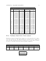
1
FEAP - - A Finite Element Analysis Program
Version 8.4 Parallel User Manual
Robert L. Taylor & Sanjay Govindjee
Department of Civil and Environmental Engineering
University of California at Berkeley
Berkeley, California 94720-1710, USA
E-Mail: [email protected] or s [email protected]
May 2013
Contents
1 Introduction
1.1 General features . . . . . . . . . . . . . . . . .
1.2 Problem solution . . . . . . . . . . . . . . . .
1.3 Graph partitioning . . . . . . . . . . . . . . .
1.3.1 METIS version . . . . . . . . . . . . .
1.3.2 ParMETIS: Parallel graph partitioning
1.3.3 Structure of parallel meshes . . . . . .
.
.
.
.
.
.
1
1
2
2
2
3
5
.
.
.
.
.
.
.
.
.
.
7
7
7
9
9
9
9
10
11
11
12
3 Solution process
3.1 Command language statements . . . . . . . . . . . . . . . . . . . . . .
3.1.1 PETSc Command . . . . . . . . . . . . . . . . . . . . . . . . . .
3.2 Solution of linear equations . . . . . . . . . . . . . . . . . . . . . . . .
3.2.1 Tolerance for iterative equation methods . . . . . . . . . . . . .
3.2.2 GLIST & GNODE: Output of results with global node numbers
3.3 Eigenproblem solution for modal problems . . . . . . . . . . . . . . . .
3.3.1 Subspace method solutions . . . . . . . . . . . . . . . . . . . . .
3.3.2 Arnoldi/Lanczos method solutions . . . . . . . . . . . . . . . .
3.4 Graphics output . . . . . . . . . . . . . . . . . . . . . . . . . . . . . . .
3.4.1 GPLOt command . . . . . . . . . . . . . . . . . . . . . . . . . .
3.4.2 NDATa command . . . . . . . . . . . . . . . . . . . . . . . . . .
3.4.3 Paraview . . . . . . . . . . . . . . . . . . . . . . . . . . . . . . .
13
14
14
15
16
16
17
18
18
19
19
20
20
.
.
.
.
.
.
.
.
.
.
.
.
.
.
.
.
.
.
.
.
.
.
.
.
.
.
.
.
.
.
.
.
.
.
.
.
.
.
.
.
.
.
.
.
.
.
.
.
2 Input files for parallel solution
2.1 Basic structure of parallel file . . . . . . . . . . . . . . . . .
2.1.1 DOMAIN - Domain description . . . . . . . . . . . .
2.1.2 FORMat - Format of matrix equations . . . . . . . .
2.1.3 BCIN BLOCked - Boundary equations in assembly .
2.1.4 LOCal to GLOBal node numbering . . . . . . . . . .
2.1.5 GETData and SENDdata - Ghost node get and send
2.1.6 MATRix storage – equation structure . . . . . . . . .
2.1.7 EQUAtion number data . . . . . . . . . . . . . . . .
2.1.8 END DOMAIN record . . . . . . . . . . . . . . . . .
2.1.9 Initial conditions . . . . . . . . . . . . . . . . . . . .
i
.
.
.
.
.
.
.
.
.
.
.
.
.
.
.
.
.
.
.
.
.
.
.
.
.
.
.
.
.
.
.
.
.
.
.
.
.
.
.
.
.
.
.
.
.
.
.
.
.
.
.
.
.
.
.
.
.
.
.
.
.
.
.
.
.
.
.
.
.
.
.
.
.
.
.
.
.
.
.
.
CONTENTS
ii
A Installation
A.1 Installing PETSc . . . . . . . . . . . . . . . . . . . . . . . . . . . . . .
A.2 Installing parallel FEAP . . . . . . . . . . . . . . . . . . . . . . . . . .
23
23
24
B Solution Command Manual
25
C Program structure
C.1 Introduction . . . . . . . . . . . . . . . . . . . . . . . . . . . . . . . . .
39
39
D Parallel Validation
D.1 Timing Tests . . . . . . . . . . . . . . . . . . . .
D.1.1 Linear Elastic Block . . . . . . . . . . . .
D.1.2 Nonlinear Elastic Block . . . . . . . . . . .
D.1.3 Plasticity . . . . . . . . . . . . . . . . . .
D.1.4 Box Beam: Shells . . . . . . . . . . . . . .
D.1.5 Linear Elastic Block: 10-node Tets . . . .
D.1.6 Transient . . . . . . . . . . . . . . . . . .
D.1.7 Mock turbine . . . . . . . . . . . . . . . .
D.1.8 Mock turbine Small . . . . . . . . . . . . .
D.1.9 Mock turbine Tets . . . . . . . . . . . . .
D.1.10 Eigenmodes of Mock Turbine . . . . . . .
D.2 Serial to Parallel Verification . . . . . . . . . . . .
D.2.1 Linear elastic block . . . . . . . . . . . . .
D.2.2 Box Beam . . . . . . . . . . . . . . . . . .
D.2.3 Linear Elastic Block: Tets . . . . . . . . .
D.2.4 Mock Turbine: Modal Analysis . . . . . .
D.2.5 Transient . . . . . . . . . . . . . . . . . .
D.2.6 Nonlinear elastic block: Static analysis . .
D.2.7 Nonlinear elastic block: Dynamic analysis
D.2.8 Plastic plate . . . . . . . . . . . . . . . . .
D.2.9 Transient plastic . . . . . . . . . . . . . .
40
41
41
41
41
42
42
43
43
44
44
45
45
45
46
47
48
51
54
55
55
56
.
.
.
.
.
.
.
.
.
.
.
.
.
.
.
.
.
.
.
.
.
.
.
.
.
.
.
.
.
.
.
.
.
.
.
.
.
.
.
.
.
.
.
.
.
.
.
.
.
.
.
.
.
.
.
.
.
.
.
.
.
.
.
.
.
.
.
.
.
.
.
.
.
.
.
.
.
.
.
.
.
.
.
.
.
.
.
.
.
.
.
.
.
.
.
.
.
.
.
.
.
.
.
.
.
.
.
.
.
.
.
.
.
.
.
.
.
.
.
.
.
.
.
.
.
.
.
.
.
.
.
.
.
.
.
.
.
.
.
.
.
.
.
.
.
.
.
.
.
.
.
.
.
.
.
.
.
.
.
.
.
.
.
.
.
.
.
.
.
.
.
.
.
.
.
.
.
.
.
.
.
.
.
.
.
.
.
.
.
.
.
.
.
.
.
.
.
.
.
.
.
.
.
.
.
.
.
.
.
.
.
.
.
.
.
.
.
.
.
.
.
.
.
.
.
.
.
.
.
.
.
.
.
.
.
.
.
.
.
.
.
.
.
.
.
.
.
.
.
.
.
.
List of Figures
1.1
Structure of stiffness matrix in partitioned equations.
. . . . . . . . .
6
2.1
Input file structure for parallel solution.
. . . . . . . . . . . . . . . . .
8
D.1 Comparison of Serial (left) to Parallel (right) mode shape 1 degree of
freedom 1. . . . . . . . . . . . . . . . . . . . . . . . . . . . . . . . . . .
D.2 Comparison of Serial (left) to Parallel (right) mode shape 2 degree of
freedom 2. . . . . . . . . . . . . . . . . . . . . . . . . . . . . . . . . . .
D.3 Comparison of Serial (left) to Parallel (right) mode shape 3 degree of
freedom 3. . . . . . . . . . . . . . . . . . . . . . . . . . . . . . . . . . .
D.4 Comparison of Serial (left) to Parallel (right) mode shape 4 degree of
freedom 1. . . . . . . . . . . . . . . . . . . . . . . . . . . . . . . . . . .
D.5 Comparison of Serial (left) to Parallel (right) mode shape 5 degree of
freedom 2. . . . . . . . . . . . . . . . . . . . . . . . . . . . . . . . . . .
D.6 Comparison of Serial (left) to Parallel (right) mode shape 1 degree of
freedom 1. . . . . . . . . . . . . . . . . . . . . . . . . . . . . . . . . . .
D.7 Comparison of Serial (left) to Parallel (right) mode shape 2 degree of
freedom 2. . . . . . . . . . . . . . . . . . . . . . . . . . . . . . . . . . .
D.8 Comparison of Serial (left) to Parallel (right) mode shape 3 degree of
freedom 3. . . . . . . . . . . . . . . . . . . . . . . . . . . . . . . . . . .
D.9 Comparison of Serial (left) to Parallel (right) mode shape 4 degree of
freedom 1. . . . . . . . . . . . . . . . . . . . . . . . . . . . . . . . . . .
D.10 Comparison of Serial (left) to Parallel (right) mode shape 5 degree of
freedom 2. . . . . . . . . . . . . . . . . . . . . . . . . . . . . . . . . . .
D.11 von Mises stresses at the end of the loading. (left) serial, (right) parallel
D.12 Z-displacement for the node located at (0.6, 1.0, 1.0). . . . . . . . . .
D.13 11-component of the stress in the element nearest (1.6, 0.2, 0.8). . . . .
D.14 1st principal stress at the node located at (1.6, 0.2, 0.8). . . . . . . . .
D.15 von Mises stress at the node located at (1.6, 0.2, 0.8). . . . . . . . . . .
iii
49
49
49
50
50
51
51
52
52
52
56
57
58
58
59
Chapter 1
INTRODUCTION
1.1
General features
This manual describes features for the parallel version of the general purpose Finite
Element Analysis Program (FEAP). It is assumed that the reader of this manual is
familiar with the use of the serial version of FEAP as described in the basic user
manual.[1] It is also assumed that the reader of this manual is familiar with the finite
element method as describe in standard reference books on the subject (e.g., The Finite
Element Method, 6th edition, by O.C. Zienkiewicz, R.L. Taylor, et al. [2, 3, 4]).
The current version of the parallel code modifies the serial version of FEAP to interface to the PETSc library system (version 3.3) available from Argonne National
Laboratories.[5, 6] In addition the METIS[7] and ParMETIS[8] libraries are used to partition each mesh for parallel solution. The present parallel version of FEAP may
only be used in a UNIX/Linux (including Mac OS X) environment and includes an
integrated set of modules to perform:
1. Input of data describing a finite element model;
2. An interface to METIS[7] to perform a graph partitioning of the mesh nodes. A
stand alone module exists to also use ParMETIS[8] to perform the graph partitioning for very large problems;
3. An interface to PETSc[5, 6, 9] to perform the parallel solution steps;
4. Construction of solution algorithms to address a wide range of applications; and
5. Graphical and numerical output of solution results.
1
CHAPTER 1. INTRODUCTION
1.2
2
Problem solution
The solution of a problem using the parallel versions starts from a standard input
file for a serial solution. This file must contain all the data necessary to define nodal
coordinate, element connection, boundary condition codes, loading conditions, and
material property data. That is, if it were possible, this file must be capable of solving
the problem using the serial version. However, at this stage of problem solving the only
solution commands included in the file are those necessary to partition the problem for
the number of processors to be used in the parallel solution steps.
1.3
Graph partitioning
To use the parallel version of FEAP it is first necessary to construct a standard input
file for the serial version of FEAP. Preparation of this file is described in the FEAP
User Manual.[1]
1.3.1
METIS version
After the file is constructed and its validity checked, a serial execution of the parallel
FEAP program built in the parfeap directory may be performed. Using the GRAPh
solution command statement followed by an OUTDomains solution command will generate the needed parallel execution input files. To use this option a basic form for the
input file is given as:
FEAP * * Start record and title
...
Control and mesh description data
...
END mesh
<Initial condition data for transient problems>
BATCh
GRAPh node numd
OUTDomains
END batch
...
STOP
! METIS partitions ’numd’ nodal domains
! Creates ’numd’ partitioned meshes
CHAPTER 1. INTRODUCTION
3
where the node on the GRAPh command is optional. Options for OUTDomains are explained below in Sect. 1.3.3 Using these commands, METIS [7] will split a problem
into numd partitions by partitioning the node graph and output numd input files for a
subsequent parallel solution of the problem.
The initial condition data is only required for transient solutions in which inital data
is non-zero. Otherwise this data is omitted. The form of the initial condition data is
described in the basic User manual.[1]
For efficiency of assembly, it is necessary to pre-allocate matrix memory requirements.
In PETSc, there are two basic matrix formats: AIJ and BAIJ. By default FEAP
stores the pre-allocation information in the partitioned input files in the AIJ format
when using OUTDomains. This format is compatible with most of PETSc’s solver options. However, if one wishes to use a solver that requires (or benefits) from the BAIJ
(blocked) format, then one can issue the command
OUTDomains,BAIJ
The block size can optionally be controlled by:
OUTDomains,BAIJ,,<nsbk>
The block size nsbk can be any (integer) factor of ndf and defaults to ndf if not
specified. Note that in the BAIJ format, degrees of freedom with Dirichlet boundary
are included in the matrix assembly. Issuing OUTDomains,AIJ forces AIJ format. In
this format it is also possible to include the degrees of freedom with Dirichlet boundary
conditions in the matrix assembly (as is required for certain PETSc solvers). This is
done by setting the boundary equation flag to unity:
OUTDomains,AIJ,1,<nsbk>
In this format, one can optionally provide PETSc with a hint to the equation block
size nsbk. As with BAIJ, this value defaults to ndf if not specified.
1.3.2
ParMETIS: Parallel graph partitioning
A stand alone parallel graph partitioner also exists.1 The parallel partitioner, partition
(located in the $(FEAPHOME8 4)/parfeap/partition subdirectory), uses ParMETIS [8]
to perform the construction of the nodal split. To use this program it is necessary to
have a FEAP input file that contains all the nodal coordinate and all the element
connection records. That is, there must be a file with the form:
1
This is only needed for problems so large that they can not be partitioned with METIS.
CHAPTER 1. INTRODUCTION
4
FEAP * * Start record and title
Control record
COORdinates
All nodal coordinate records
...
ELEMent
All element connection records
...
remaining mesh statemnts
...
END mesh
The flat form for an input file may be created from any FEAP input file using the
solution command:
OUTMesh
This creates an input file with the same name and the extender ”.rev”. If a TIE
mesh manipulation command is used the output mesh will remove unused nodes and
renumber the node numbers.
Once the flat input file exists a parallel partitioning is performed by executing the
command
mpirun -n nump partition numd Ifile
where nump is the number of processors that ParMETIS uses, numd is the number of
mesh partitions to create and Ifile is the name of the flat FEAP input file. For
an input file originally named Ifile, the program creates a graph file with the name
graph.file. The graph file contains the following information:
1. The processor assignment for each node (numnp)
2. The pointer array for the nodal graph (numnp+1)
3. The adjacency lists for the nodal graph
To create the partitioned mesh input files the flat input file is used again (in the
same directory containing the graph.file) in a serial execution of the parallel FEAP
together with the solution commands
CHAPTER 1. INTRODUCTION
5
GRAPh FILE
OUTDomains
See the next section for a discussion of possible options for OUTDomains.
It is usually also possible to also create the graph.file in parallel without separately
running partition from the command line by using the command set
OUTMesh
GRAPh PARTition numd
OUTDomains
where numd is the number of domains to create. For this to work the program mpirun
must be in your path. Here, the parameter nump is equal to numd.2 The use of the
command OUTMesh is required to ensure that a flat input file is available and after
execution it is destroyed.
1.3.3
Structure of parallel meshes
It is assumed that numd represents the number of processors to be used in the parallel
solution. Each partition is assigned numpn nodes. The number can differ slightly among
the various partitions but is approximately the total number of nodes in the problem
divided by numd. In the current release, no weights are assigned to the node or the node
graph edges to reflect possible differences in solution or communication effort. Each
partitioned input file also contains ghost nodes for effecting the evaluation of element
residuals. The sum of the nodes in a partition (numpn) and its ghost nodes defines the
total number of nodes in each partitioned data file (i.e., the total number of nodes,
numnp, in each mesh partition).
In the parallel solution the global equations are numbered sequentially from 1 to the
total number of equations in the problem (numteq). The nodes in partition 1 are
associated with the first set of equations, the nodes in partition 2 the second set, etc.
For each partition, the stiffness and/or the mass matrix is also partitioned and each
partition matrix has two parts: (a) a diagonal block for all the nodes in the partition
(i.e., numpn nodes) and, (b) off diagonal blocks associated with the ghost nodes as
shown in Figure 1.1. In solving a set of linear equations
K du = R
associated with an implicit solution step, the solution vector du and the residual R
are also split according to each partition. The residual for each partition contains only
2
Use of this command set requires the path to the location of the partition program to be set in
the pstart.F file located in the parfeap directory.
CHAPTER 1. INTRODUCTION
6
the terms associated with the equations of the partition. The solution vector, however,
has both the terms associated with the partition as well as those associated with the
equations of its ghost nodes. In this way, it is only necessary to exchange values for the
displacement quantities associated with the respective ghost nodes after each solution
iteration. This optimizes the communication costs.
In the next chapter we describe how the input data files for each partition are organized.
K11
K1g
K2g
K22
K
3g
Processor 1
K2g
K
33
Processor 2
K
3g
Processor 3
Figure 1.1: Structure of stiffness matrix in partitioned equations.
Chapter 2
Input files for parallel solution
After using the METIS or the ParMETIS partitioning algorithm on the total problem
(for example, that given by say the mesh file Ifilename) FEAP produces numd files
for the partitions and these serve as input for the parallel solution. Each new input
file is named Ifilename 0001, etc. up to the number of partitions specified (i.e., numd
partitions).
The first part of each file contains a standard FEAP input file for the nodes and
elements belonging to the partition. This is followed by a set of commands that begin
with DOMAin and end with END DOMAin. All of the data contained between the DOMAin
and END DOMAin is produced automatically by FEAP when using OUTDomains.
The file structure for a parallel solution is shown in Figure 2.1 and is provided only to
describe how the necessary data is given to each partition. No changes are allowed to
be made to these statements.
2.1
Basic structure of parallel file
Each part of the data following the END MESH statement performs a specific task in the
parallel solution. It is important that the data not be altered in any way as this can
adversely affect the solution process. Below we describe the role each data set plays
during the solution.
2.1.1
DOMAIN - Domain description
The DOMAIN data defines the number of nodes belonging to this partition (numpn), the
number of total nodes in the problem (numtn) and the number of total equations in the
7
CHAPTER 2. INPUT FILES FOR PARALLEL SOLUTION
FEAP * * Start record and title
...
Control and mesh description data for a partition
...
END MESH
DOMAin
numpn
numtn
numteq
FORMat <AIJ,BAIJ>
<BCIN BLOCked nsbk>
(Required for BAIJ)
LOCAl to GLOBal node numbers
...
GETData POINter
...
nget_pnt
GETData VALUes
...
nget_val
SENDdata POINter
...
nsend_pnt
SENDdata VALUes
...
nsend_val
MATRix storage
...
<EQUAtion> numbers (If BCIN is not present)
...
END DOMAIN
BATCh ! Optional initial conditions
INITial DISPlacements
END BATCH
... List of initial conditions
INCLude solve.filename
STOP
Figure 2.1: Input file structure for parallel solution.
8
CHAPTER 2. INPUT FILES FOR PARALLEL SOLUTION
9
problem (numteq). Note that the number of nodes in the partition (numpn) is always
less or equal to the number of nodes given on the control record (numnp) due to the
presence of the ghost nodes. The sum over all partitions of the number of nodes in
each partition (numpn) is equal to the total number of nodes in the problem (numtn).
2.1.2
FORMat - Format of matrix equations
This data set defines the format assumed for the matrix pre-allocation data as well as
the local to global node number data. The valid options are AIJ and BAIJ; AIJ is the
default.
2.1.3
BCIN BLOCked - Boundary equations in assembly
This data set is optional. For matrix formats that include the degrees of freedom
associated with Dirichlet boundary conditions in the matrix assembly, this command
will be present. It takes a single numerical parameter indicating the blocking size which
is always an (integer) factor of ndf.
2.1.4
LOCal to GLOBal node numbering
Each record in this set defines three values: (1) a local node number in the partition;
(2) the global node associated with the local number; and (3) the global equation block
number associated with the local node. The first numpn records in the set are the nodes
associated with the current partition the remaining records with the ghost nodes.
2.1.5
GETData and SENDdata - Ghost node get and send
The current partition retrieves (GETData) the solution values for its ghost nodes from
other partitions. The data is divided into two parts: (1) A POINTER part which defines
the number of values to obtain from each partition and (2) The VALUes list of local
node numbers needing values. The pointer data is given as
GETData POINter nparts
np_1
np_2
...
np_nparts
CHAPTER 2. INPUT FILES FOR PARALLEL SOLUTION
10
where np i defines the number of values to get from partition-i (note the number should
always be a zero for the current partition). The nodal values list is given as
GETData VALUes nvalue
local_node_1
local_node_2
...
local_node_nvalue
The local node i numbers are grouped so that the first np 1 are obtained from processor 1, the next np 2 from processor 2, etc. The local node 1 is the number of a
local ghost node to be obtained from another processor and may appear only once in
the list of GETData VALUes.
A corresponding pair of lists is given for the data to be sent (SENDdata) to the other
processors. The lists have identical structure to the GETData lists and are given by
SENDdata POINter nparts
np_1
np_2
...
np_nparts
and
SENDdata VALUes nvalue
local_node_1
local_node_2
...
local_node_nvalue
where again the local node i numbers are grouped so that the first np 1 are sent to
processor 1, the next np 2 to processor 2, etc. It is possible for a local node number
to appear more than once in the SENDdata VALUes list as it could be a ghost node for
more than one other partition. np i should be zero for input file Ifilename 000i.
2.1.6
MATRix storage – equation structure
Each equation in the global matrix consists of the number of terms that are associated
with the current partition and the number of terms associated with other partitions.
This information is provided for each equation (or equation block when in BAIJ format)
CHAPTER 2. INPUT FILES FOR PARALLEL SOLUTION
11
by the MATRix storage data set. Each record in the set is given by the global equation
number followed by the number of terms associated with the current partition and then
the number of terms associated with other partitions. The use of this data is critical to
obtain rapid assembly of the global matrices by PETSc. If it is incorrect the assembly
time will be very large compared to the time needed to compute the matrix coefficients
or even solve the equations.
When the matrix format is BAIJ the data is given for each block equation. Thus, the
first nsbk equations are associated with block 1, the second with block 2, etc. The
total number of equations numteq for this form is numtn × nsbk. Here, each record of
the MATRix storage data is given by the global block number, the number of blocks
associated with the current partition and the number of blocks associated with other
partitions.
When the optional BCIN command is present, every node has ndf equations independent
of any boundary conditions. If a degree-of-freedom (DOF) is of displacement type we
assemble a unit value on the diagonal and all off-diagonal entries are zero. That is, the
equations for any DOF a that are fixed will be assembled as:
1 dua = Ra = dū
where dū denotes a specified valued for the solution. In some cases, this can improve the
efficiency of the solver and for some solvers it is required, e.g. the Prometheus multigrid pre-conditioner and GAMG the geometric-algebraic multi-grid pre-conditioner.
2.1.7
EQUAtion number data
This data set is not present when the boundary equations are assembled (BCIN). However, when the equations are in AIJ format and BCIN has not been set, then it is
necessary to fully describe the equation numbering associated with each node in the
partition. This is provided by the EQUAtion number data set. The set consists of
numnp records which contain the local node number followed by the global equation
number for every degree-of-freedom associated with the node. If a degree-of-freedom
is restrained (i.e., of displacement or Dirichlet type) the equation is not active and a
zero appears. This form results in fewer unknown values but may not be used with
any equation solution requiring all equations to be present (in particular, Prometheus
and GAMG).
2.1.8
END DOMAIN record
The parallel domain data is terminated by the END DOMAIN record. It is followed by
the solution commands.
CHAPTER 2. INPUT FILES FOR PARALLEL SOLUTION
2.1.9
12
Initial conditions
Following the domain data the list of any initial conditions applied to a transient
problem will appear. The initial conditions must be fully specified in the original input
data file.
Initial conditions for displacements will appear as shown in Fig. 2.1. However, if rate
type conditions are applied the data will appear as
BATCh
! Initial rate conditions
TRANsient type c1 c2 c3
INITial RATE
END BATCH
.... List of rate conditions
where type is one of the standard feap transient solution algorithms and c1,c2,c3 are
the values of the transient solution parameters. For example, if the Newmark method
is used then type will be output as NEWMark and c1,c2 will be the values of the β, γ
Newmark parameters. The final parameter c3 is not used by Newark but appears as
unity.
If both initial displacements and intial rates are specified then both BATCh--END pairs
of data will appear in the domain input file.
Chapter 3
Solution process
Once the parallel input mesh files are created an execution of the parallel version of
feap may be performed using, for example, the command line statement
mpirun -n $NPROC $FEAPHOME8_4/parfeap/feap -ksp_type cg -pc_type jacobi
or the command line statement
mpirun -n $NPROC $FEAPHOME8_4/parfeap/feap -ksp_type cg -pc_type prometheus
(for details on using other solvers as well as optional parameters for these choices
see the makefile in the parfeap subdirectory). The parameters setting the number
of processors (NPROC) and the execution path (FEAPHOME8 4) must be defined before
issuing the command. This can be done by setting shell environment variables.
Once parallel FEAP starts, the input file should be set to Ifilename 0001 where
filename is the name of the solution file to be solved. Each processor reads its input
file up to the END DOMAIN statement and then starts processing command language
statements.
In a parallel solution using FEAP the same command language statements must be
provided for each partition. This is accomplished by the statement
INCLude solve.filename
appearing after the END DOMAin statement, where filename is the name of the input
data file with the leading I and the trailing partition number removed. Thus for the file
named Iblock 0001 the command is given as solve.block. All solution commands
are then placed in a file with this name and can include both BATCh and INTEractive
commands. For example a simple solution may be given by the commands
13
CHAPTER 3. SOLUTION PROCESS
14
BATCh
PETSc ON
TOL ITER 1.d-07 1.d-08 1.d+20
TANGent,,1
END
INTEractive
placed in the solve.filename file. Note that both batch and interactive modes of
solution are optionally included. Interactive commands need only be entered once and
are sent to other processors automatically. In the subsequent subsections we describe
some of the special commands that control the parallel execution mode of FEAP
3.1
Command language statements
Most of the standard command language statements available in the serial version of
FEAP (see users manual [1]) may be used in the parallel version of feap. New commands are available also that are specifically related to performing a parallel solution.
3.1.1
PETSc Command
The PETSc command is used to activate the parallel solution process. The command
PETSc <ON,OFF>
may be used to turn on and off the parallel execution. It is only required for single
processor solutions and is optional when two or more processors are used in the solution process. When required, it should always be the first solution command. It is
automatically included in the default solve.filename generated by OUTDomains.
The command may also be used with the VIEW parameter to create outputs for the
tangent matrix, solution residual or mass matrix. Thus, use as
PETSc VIEW
MASS
PETSc NOVIew
will create a file named mass.m that contains all the non-zero values of the total mass
matrix. The parameter VIEW turns on output arrays and this remains in effect for all
CHAPTER 3. SOLUTION PROCESS
15
commands until the command is given with the NOVIew parameter. The file is created
in a format that may be directly used by MATLAB.[11] This command should only be
used with small problems to verify the correctness of results as large files will result
otherwise.
3.2
Solution of linear equations
The parallel version of FEAP can use most all of the SLES (linear solvers) available in
PETSc as well as the parallel multigrid solvers, Prometheus[10] and GAMG. This also
includes most of the direct solvers that can optionally be built with PETSc. The actual
type of linear solver used is specified on the mpirun line and several useful examples
are contained in the makefile located in the parfeap directory (see, Sect. 3 above).
Once the solution is initiated the solution of linear equations is performed whenever a
TANG,,1 or SOLVe command is given.
The types of solvers and the associated pre-conditioners tested to date are described
in Table 3.1. This is only a small sampling of the many options available in PETSc.
Solver
CG
CG
CG
CG
CG
Preconditioner
Jacobi
Prometheus
Hypre with Boomerang
ML/Trilinos
GAMG
MINRES
MINRES
GMRES
GMRES
GMRES
GMRES
SuperLU
Jacobi
Prometheus
Jacobi
Prometheus
Block Jacobi
ASM(ILU)
(direct)
Spooles
MUMPS
(direct)
(direct)
Matrix format/Notes
AIJ and BAIJ formats
BAIJ format
AIJ format
AIJ format
Successor to Prometheus, AIJ with BCIN
format
AIJ and BAIJ formats
BAIJ format
AIJ and BAIJ formats
BAIJ format
Often gives indefinite factor.
AIJ format (has BLAS conflict on Mac OS
X ≥ 10.7.5)
AIJ format
AIJ format
Table 3.1: Linear solvers and pre-conditioners tested.
The solvers, together with the necessary options for preconditioning are specified on
the mpirun line. For convenience, it is recommended to place these in the provided
CHAPTER 3. SOLUTION PROCESS
16
makefile and to run them with the make command. Several options are pre-provided
in the distributed makefile.
3.2.1
Tolerance for iterative equation methods
The basic form of iterative solution for linear equations in PETSc is a Krylov subspace
scheme. These methods terminate their iterations based on assumed tolerances and
can be changed as desired.
Termination tolerances for the solvers are given by either
TOL ITER rtol atol dtol
or
ITER TOL rtol atol dtol
where rtol is the tolerance for the preconditioned equations, atol the tolerance for
the original equations and dtol a value at which divergence is assumed. The default
values are:
rtol = 1.d − 8 ;
atol = 1.d − 16 and dtol = 1.d + 16
For many problems it is advisable to check that the actual solution is accurate when
using iterative methods since termination of the iterative solution is performed based
on the rtol value. A check should be performed using the command sequence
TANG,,1
LOOP,,1
FORM
SOLV
NEXT
since the TANG command has significant set up costs, especially for multi-grid methods.
Indeed, for some problems more than one iteration is needed in the loop.
3.2.2
GLIST & GNODE: Output of results with global node
numbers
In normal execution each partition creates its own output file (e.g., Ofilename 0001,
etc.) with printed data given with the local node and element numbers of the processor’s input data file. In some cases the global node numbers are known and it is desired
CHAPTER 3. SOLUTION PROCESS
17
to identify which processor to which the node is associated. This may be accomplished
by including a GLISt command in the solution statements along with the list of global
node numbers to be output. The option is restricted to 3 lists, each with a maximum
of 100 nodes. The command sequence is given by:
BATCh
GLISt,,<1,2,3>
END
list of global node numbers, 8 per record
! blank termination record
The list will be converted by each processor into the local node numbers to be output
using the command
DISP LIST <1,2,3>
The command may also be used with VELOcity, ACCEleration, and STREss; see the
relevant manual pages in the FEAP Users Manual.[1]
It is also possible to directly output the global node number associated with individual
local node numbers using the command statement
DISP GNODe nstart nend ninc
where nstart and nend are global node numbers. This command form also may be
used with VELOcity, ACCEleration, and STREss.
3.3
Eigenproblem solution for modal problems
The computation of the natural modes and frequencies of free vibration of an undamped
linear structural problem requires the solution of the general linear eigenproblem
KΦ = MΦΛ
In the above K and M are the stiffness and mass matrices, respectively, and Φ and Λ
are the normal modes and frequencies squared. Normally, the constraint
ΦT M Φ = I
is used to scale the eigenvectors. In this case one also obtains the relation
ΦT K Φ = Λ
CHAPTER 3. SOLUTION PROCESS
3.3.1
18
Subspace method solutions
The subspace algorithm contained in FEAP has been extended to solve the above
problem in a parallel mode. The use of the subspace algorithm requires a linear solution
of the equations
Kx = y
for each vector in the subspace and for each subspace iteration. The parallel subspace
solution is performed using the command set
TANGent
MASS <LUMPed,CONSistent>
PSUBspace <print> nmodes <nadded>
where nmodes is the desired number of modes, nadded is the number of extra vectors
used to accelerate the convergence (default is maximum of nmodes and 8) and print
produces a print of the subspace projections of K and M. The accuracy of the computed eigenvalues is the maximum of 1.d − 12 and the value set by the TOL solution
command. The method may be used with either a lumped or a consistend mass matrix.
If it is desired to extract 10 eigenvectors with 8 added vectors and 20 iterations are
needed to converge to an acceptable error it is necessary to perform 360 solutions of the
linear equations. Thus, for large problems the method will be very time consuming.
3.3.2
Arnoldi/Lanczos method solutions
In order to reduce the computational effort for eigenproblems the Arnoldi/Lanczos
methods implemented in the ARPACK module available from Rice University[12] has
been modified to work with the parallel version of FEAP.
Two modes of the ARPACK solution methods are included in the program:
1. Mode 1: Solves the problem reformed as
M−1/2 K M−1/2 Ψ = Ψ Λ
where
Φ = M−1/2 Ψ
This form is most efficient when the mass matrix is diagonal (lumped) and, thus,
in the current release of parallel FEAP is implemented only for diagonal (lumped)
mass forms. This mode form is specified by the solution command set
CHAPTER 3. SOLUTION PROCESS
TANGent
MASS LUMPed
PARPack LUMPed
19
nmodes <maxiters> <eigtol>
where nmodes is the number of desired modes. Optionally, maxiters is the
number of iterations to perform (default is 300) and eigtol the solution tolerance
on eigenvalues (default is the maximum of 1.d − 12 and the values set by the
command TOL).
2. Mode 3: Solves the general linear eigenproblem directly and requires solution of
the linear problem
Kx = y
for each iteration. Fewer iterations are normally required than in the subspace
method, however, the method is generally far less efficient than the Mode 1 form
described above. This form is given by the set of commands
TANGent
MASS <LUMPed,CONSistent>
PARPack <SYMMetric> nmodes <maxiters> <eigtol>
Use of the command MASS alone also will employ a consistent mass (or the mass
produced by the quadrature specified).
3.4
Graphics output
During a solution the graphics commands may be given in a standard manner. However,
each processor will open a graphics window and display only the parts that belong to
that processor. Scaling is also done processor by processor unless the PLOT RANGe
command is used to set the range for the plot values.
3.4.1
GPLOt command
An option does exist to collect all the results together and present on a single graphics
window. This option also permits postscript outputs to be constructed and saved in
files. To collect the results together it is necessary to write the results to disk for each
item to be graphically presented. This is accomplished using the GPLOt command.
This command has the options
GPLOt DISPlacement n
GPLOt STREss
n
GPLOt PSTRess
n
CHAPTER 3. SOLUTION PROCESS
20
where n denotes the component of a displacement (DISP), nodal stress (STRE) or principal stress (PSTRE). Each use of the command creates a file for each processor with
the form
Gproblem_domain.xyyyy
where problem domain is the name of the problem file for the domain; x is d, s or p
for a displacement, stress or principal stress, respectively; and yyyy is a unique plot
number (it will be between 0001 and 9999).
3.4.2
NDATa command
Once the GPLOt files have been created they may be plotted using a serial execution of
the parallel FEAP program (i.e., using the original pre-partioning step file Ifilename).
The command may be given in INTEractive mode only as one of the options:
Plot > NDATa DISPl
n
Plot > NDATa STREss n
Plot > NDATa PSTRess n
where n is the value of yyyy used to write the file.
WARNING: Plots by FEAP use substantial memory and thus this option may not
work for very large problems. One should minimize the number of commands used
during input of the problem description (i.e., remove input commands in the mesh
that create new memory).
3.4.3
Paraview
An alternate scheme for plotting parallel solutions can be achieved by use of the Paraview1 system. This is a convenient open source tool that can be used with FEAP.
This integration is provided as a user macro extension to the program and can be
downloaded from http://www.ce.berkeley.edu/∼sanjay/FEAP/feap.html.
1
See http://www.paraview.org.
Bibliography
[1] R.L. Taylor. FEAP - A Finite Element Analysis Program, User Manual. University of California, Berkeley.
.
http://www.ce.berkeley.edu/feap.
[2] O.C. Zienkiewicz, R.L. Taylor, and J.Z. Zhu. The Finite Element Method: Its
Basis and Fundamentals. Elsevier, Oxford, 6th edition, 2005.
[3] O.C. Zienkiewicz and R.L. Taylor. The Finite Element Method for Solid and
Structural Mechanics. Elsevier, Oxford, 6th edition, 2005.
[4] O.C. Zienkiewicz, R.L. Taylor, and P. Nithiarasu. The Finite Element Method for
Fluid Dynamics. Elsevier, Oxford, 6th edition, 2005.
[5] S. Balay, K. Buschelman, W.D. Gropp, D. Kaushik, M.G. Knepley,
L.C. McInnes, B.F. Smith, and H. Zhang.
PETSc Web page, 2001.
http://www.mcs.anl.gov/petsc.
[6] S. Balay, K. Buschelman, V. Eijkhout, W.D. Gropp, D. Kaushik, M.G. Knepley,
L.C. McInnes, B.F. Smith, and H. Zhang. PETSc users manual. Technical Report
ANL-95/11 - Revision 2.1.5, Argonne National Laboratory, 2004.
[7] G. Karypis. METIS: Family of multilevel partitioning algorithms. http://wwwusers.ce.umn.edu/˜karypis/metis/.
[8] G. Karypis. ParMETIS parallel graph partitioning. (see internet address:
http://www-users.cs.unm.edu/~karypis/metis/parmetis/), 2003.
[9] S. Balay, W.D. Gropp, L.C. McInnes, and B.F. Smith. Efficient management
of parallelism in object oriented numerical software libraries. In E. Arge, A. M.
Bruaset, and H. P. Langtangen, editors, Modern Software Tools in Scientific Computing, pages 163–202. Birkhäuser Press, 1997.
[10] M. Adams. PROMETHEUS: Parallel multigrid solver library for unstructured
finite element problems. http://www.columbia.edu/˜ma2325.
21
BIBLIOGRAPHY
22
[11] MATLAB. www.mathworks.com, 2011.
[12] R. Lehoucq, K. Maschhoff, D. Sorensen, and C. Yang. ARPACK: Arnoldi/lanczos
package for eigensolutions. http://www.caam.rice.edu/software/ARPACK/.
[13] J. Demmel, J. Dongarra, and et al. LAPACK – Linear Algebra PACKage, June
2010. http://netlib.org/lapack.
[14] G. Karypis. ParMETIS parallel graph partitioning. (see internet address:
http://www-users.cs.unm.edu/~karypis/metis/parmetis/), 2003.
[15] R.L. Taylor. FEAP - A Finite Element Analysis Program, Installation Manual.
University of California, Berkeley.
. http://www.ce.berkeley.edu/feap.
Appendix A
Installation
The installation of the parallel version of FEAP is accomplished after first building
a serial version (see FEAP Installation Manual for instructions to build the serial
version).
A.1
Installing PETSc
In order to build the parallel version it is necessary to have an installed version of
PETSc[5, 6] that includes Metis, and ParMetis[14] . It is further important to install
several of the optional pre-conditioner and solver packages.
In the appropriate “.bash xxx” file it is useful (but not necessary) to insert lines similar
to
export PETSC_DIR=/Users/rlt/Software/petsc-3.3-p5
export PETSC_ARCH=gnu-opt
This saves on some typing later on.
The files, manuals, and installation instruction for PETSc may be downloaded from:
http://www.mcs.anl.gov/petsc
However in short, after downloading and unpacking the source file the PETSc libraries
need to be built (and tested). Our typical (non-debugging) installation is performed
as follows:
23
APPENDIX A. INSTALLATION
24
export PETSC_DIR=/Users/rlt/Software/petsc-3.3-p5
export PETSC_ARCH=gnu-opt
cd $PETSC_DIR
./configure --download-{spooles,parmetis,superlu_dist,prometheus, \
mpich,ml,hypre,metis,mumps,scalapack,blacs} --with-debugging=0
Once the configuration is completed the PETSc library is compiled using:
make PETSC_DIR=/Users/rlt/Software/petsc-3.3-p5 PETSC_ARCH=gnu-opt all
and tested using
make PETSC_DIR=/Users/rlt/Software/petsc-3.3-p5 PETSC_ARCH=gnu-opt test
This will create a PETSc system that includes Metis, ParMetis, Spooles, SuperLU,
MUMPS, Prometheus, ML/Trilinos, Hypre as well as an MPI environment. (ScaLapack
and BLACS are needed by MUMPS.) Of these only Metis and ParMetis are required –
assuming you already have an MPI environment. Leave off the --with-debugging=0
flag if you want to build a debugging version. In general it is best to build both a
debugging and non-debugging version.
The above instructions assume use of a bash shell. For other operating systems or
shells see the PETSc documentation at [6]. Not all the listed packages are needed but
these tend to be useful for a wide variety of problem classes.
A.2
Installing parallel FEAP
Optionally one can include the ARPAck modules in the build. To do so, first build the
archive archivelib.a in the directory packages/arpack/archive using the command
make install. Then build the archive parpacklib.a in the directory parfeap/packages/arpack
using the command make install.
With the PETSc libraries available the parallel executable for FEAP is built from the
parfeap subdirectory using the command
make install
If the ARPAck libraries have been built one should edit the makefile to ensure that
they are linked by uncommenting the appropriate lines.
Appendix B
Solution Command Manual Pages
FEAP has a few options that are used only to solve parallel problems. The commands
are additions to the command language approach in which users write each step using
available commands. The following pages summarize the commands currently added
to the parallel version of FEAP.
25
APPENDIX B. SOLUTION COMMAND MANUAL
DISPlacements
26
FEAP COMMAND INPUT COMMAND MANUAL
disp,gnod,<n1,n2,n3>
Other options of this command are described in the FEAP User Manual. The command DISPlacement may be used to print the current values of the solution generalized
displacement vector associated with the global node numbers of the original mesh. The
command is given as
disp,gnod,n1,n2,n3
prints out the current solution vector for global nodes n1 to n2 at increments of n3
(default increment = 1). If n2 is not specified only the value of node n1 is output. If
both n1 and n2 are not specified only the first node solution is reported.
APPENDIX B. SOLUTION COMMAND MANUAL
GLISt
27
FEAP COMMAND INPUT COMMAND MANUAL
glist,,n1
<values>
The command GLISt is used to specify lists of global node numbers for output of
nodal values. It is possible to specify up to three different lists where the list number
corresponds to n1 (default = 1). The list of nodes to be output is input with up to
8 values per record. The input terminates when less than 8 values are specified or a
blank record is encountered. No more than 100 items may be placed in any one list.
List outputs are then obtained by specifying the command:
name,list,n1
where name may be DISPlacement,VELOcity,ACCEleration, or STREss and n1 is the desired
list number.
Example:
BATCh
GLISt,,1
END
1,5,8,20
BATCh
DISP,LIST,1
...
END
The global list of nodes is processed to determine the processor and the associated
local node number. Each processor then outputs its active values (if any) and gives
both the local node number in the partition as well as the global node number.
APPENDIX B. SOLUTION COMMAND MANUAL
GPLOt
gplo
gplo
gplo
gplo
28
FEAP COMMAND INPUT COMMAND MANUAL
disp
velo
acce
stre
n
n
n
n
Use of plot commands during execution of the parallel version of FEAP create the same
number of graphic windows as processors used to solve the problem. Each window
contains only the part of the problem contained on that processor.
The use of the GPLOt command is used to save files containing the results for all nodal
dispacements, velocities, accelerations or stresses in the total problem. The only action
occuring after the use of this command is the creation of a file containing the current
results for the quantity specified. Repeated use of the command creates files with
different names.
These results may be processed by a serial run of the problem using the mesh for the
total problem. To display the nodal values command NDATa is used. See manual page
on NDATa.
APPENDIX B. SOLUTION COMMAND MANUAL
GRAPh
29
FEAP COMMAND INPUT COMMAND MANUAL
grap,,num d
grap node num d
grap file
grap part num d
The use of the GRAPh command activates the interface to the METIS multilevel partioner. The graph partition into num d parts is performed based on a nodal graph. The
nodal partition divides the total number of nodes (i.e., numnp values) into num d nearly
equal parts.
If the GRAPh command is given with the option file the graph data is input from the
file graph.filename where filename is the same as the input file without the leading
I character. The data contained in the graph.filename is created using the stand
alone partitioner program which employs the PARMETIS multilevel partitioner.
It is also possible to execute PARMETIS to perform the partitioning directly during
a mesh input. It is necessary to have a mesh which contains all the nodal coordinate
and element data in the input file. This is accomplished using the command set
OUTMesh
GRAPh PARTition num_d
OUTDomains
where num d is the number of domains to create. The command OUTMesh creates a
file with all the nodal and element data and is destroyed after execution of the GRAPh
command.
APPENDIX B. SOLUTION COMMAND MANUAL
ITERative
30
FEAP COMMAND INPUT COMMAND MANUAL
iter,,,icgit
iter,bpcg,v1,icgit
iter,ppcg,v1,icgit
iter,tol,v1,v2,v3
The ITERative command sets the mode of solution to iterative for the linear algebraic
equations generated by a TANGent. Currently, iterative options exist only for symmetric,
positive definite tangent arrays, consequently the use of the UTANgent command should
be avoided. An iterative solution requires the sparse matrix form of the tangent matrix
to fit within the available memory of the computer.
Serial solutions
In the serial version the solution of the equations is governed by the relative residual for
the problem (i.e., the ratio of the current residual to the first iteration in the current
time step). The tolerance for convergence may be set using the ITER,TOL,v1,v2 option.
The parameter v1 controls the relative residual error given by
1/2
(RT R)i
1/2
≤ v1 (RT R)0
and, for implementations using PETSc the parameter v2 controls the absolute residual
error given by
1/2
(RT R)i ≤ v2
The default for v1 is 1.0d-08 and for v2 is 1.0d-16. By default the maximum number
of iterations allowed is equal to the number of equations to be solved, however, this
may be reduced or increased by specifying a positive value of the paramter icgit.
The symmetric equations are solved by a preconditioned conjugate gradient method.
Without options, the preconditioner is taken as the diagonal of the tangent matrix.
Options exist to use the diagonal nodal blocks (i.e., the ndf × ndf nodal blocks, or
reduced size blocks if displacement boundary conditions are imposed) as the preconditioner. This option is used if the command is given as ITERative,BPCG. Another option
is to use a banded preconditioner where the non-zero profile inside a specified half band
is used. This option is used if the command is given as ITERative,PPCG,v1, where v1 is
the size of the half band to use for the preconditioner.
The iterative solution options currently available are not very effective for poorly conditioned problems. Poor conditioning occurs when the material model is highly non-
APPENDIX B. SOLUTION COMMAND MANUAL
31
linear (e.g., plasticity); the model has a long thin structure (like a beam); or when
structural elements such as frame, plate, or shell elements are employed. For compact
three dimensional bodies with linear elastic material behavior the iterative solution is
often very effective.
Another option is to solve the equations using a direct method (see, the DIREct command language manual page).
Parallel solutions
For the parallel version the control of the PETSc preconditioned iterative solvers is
controlled by the command
ITER TOL itol atol dtol
where itol is the tolerance for the preconditioned equations (default 1.d − 08), atol
is the tolerance for the original equations (default 1.d − 16) and dtol is a divergence
protection when the equations do not converge (default 1.d + 16).
APPENDIX B. SOLUTION COMMAND MANUAL
NDATa
32
FEAP COMMAND INPUT COMMAND MANUAL
ndat
ndat
ndat
ndat
disp
velo
acce
stre
n
n
n
n
This command is used in a serial execution of parallel FEAP using the mesh for the
total problem. It is necessary for files to be created during a parallel execution using
the GPLOt command (See manual page on GPLOt).
The command is given by
NDATa DISPlacement num
where the parameter num is the number corresponding to the order the DISPlacement
are created. Thus, the command sequence
NDATa DISPlacement 2
NDATa STREss
2
would display the results for the second files created for the displacements and stresses.
Note this command is Plot level command.
APPENDIX B. SOLUTION COMMAND MANUAL
OUTDomains
33
FEAP COMMAND INPUT COMMAND MANUAL
outd,<aij>
outd,aij,1,<bsize>
outd,baij,,<bsize>
The use of the OUTDomains command may only be used after the GRAPh command
partitions the mesh into num d parts (see GRAPh command language page for details).
Using the command OUTDomains,AIJ or OUTDomains,BAIJ creates num d input files
for a subsequent parallel solution in which the matrix format will be created in AIJ or
BAIJ format, respectively; AIJ is the default.
The parameter bsize defines the block size and must be an integer divisor of ndf.
That is if ndf = 6 then bsize may be 1, 2, 3, or 6. By default each block in the
equations has a size ndf. The setting of the block size can significantly reduce the
amount of storage needed to store the sparse coefficient matrix created by TANGent
or UTANgent when a problem has a mix of element types and the matrix is in BAIJ
format. For example if a problem has a large number of solid elements with 3 degrees
of freedom per node and additional frame or shell elements with 6 degrees of freedom
per node, specifying bsize = 3 can save considerable memory. Further the setting of
the block size can improve the rate of convergence of iterative and direct solvers.
The use of the unity flag in OUTDomains,AIJ,1 forces the inclusion of all, even prescribed, degrees of freedom in the matrix assembly for AIJ format. This permits the
use of blocking for AIJ format matrices – something that is in general not possible if
prescribed degrees of freedom are not assembled. This is the default behavior for BAIJ
format matrices.
APPENDIX B. SOLUTION COMMAND MANUAL
PETSc
pets
pets
pets
pets
pets
34
FEAP COMMAND INPUT COMMAND MANUAL
on
off
view
noview
The use of the PETSc command activates(on) or deactivates(off) parallel solution options, respectively. To turn on parallel computing the command may be given in the
simple form: PETSc. When more than one partition is created, i.e., the number of
solution processors is 2 or more, the PETSc option is on by default. The command
must be the first command of the command language program when only 1 processor
is used.
The option PETSc VIEW will result in the creation of debug files containing important
parallel matrices and vectors. The output is in MATLAB sparse format. This option
should only be used for very small problems to check that a formulation produces
correct results (i.e., there is another set of terms to which a comparison is to be made).
The option is turned off using the statement PETSc NOVIew. The default is NOVIew.
APPENDIX B. SOLUTION COMMAND MANUAL
STREss
35
FEAP COMMAND INPUT COMMAND MANUAL
stre,gnod,<n1,n2,n3>
Other options for this command are given in the FEAP User Manual. The STREss
command is used to output nodal stress results at global node numbers n1 to n2 at
increments of n2 (default = 1).
The command specified as:
stre,gnode,n1,n2,n3
prints out the stresses for global nodes n1 to n2 at increments of n3 (default increment
= 1). If n2 is not specified only the value of node n1 is output. If both n1 and n2 are
not specified only the first node solution is reported.
APPENDIX B. SOLUTION COMMAND MANUAL
TOLerance
36
FEAP COMMAND INPUT COMMAND MANUAL
tol,,v1
tol,ener,v1
tol,emax,v1
tol,iter,v1,v2,v3
The TOL command is used to specify the solution tolerance values to be used at various
stages in the analysis. Uses include:
1. Convergence of nonlinear problems in terms of the norm of energy in the current
iterate (the inner, dot, product of the displacement increment and the solution
residual vectors).
2. Convergence of iterative solution of linear equations.
3. Convergence of the subspace eigenpair solution which is measured in terms of the
change in subsequent eigenvalues computed.
The basic command, TOL,,tol, without any arguments sets the parameter tol used in
the solution of non-linear problems where the command sequence
LOOP,,30
TANG,,1
NEXT
is given. In this case, the loop is terminated either when the number of iterations
reaches 30 (or whatever number is given in this position) or when the energy error is
less than tol. The energy error is given by
Ei = (duT R)i ≤ tol (duT R)0 = E0
in which R is the residual of the equatons and du is the solution increment. The default
value of tol for the solution of nonlinear problems is 1.0d-16.
The TOL command also permits setting a value for the energy below which convergence
is assumed to occur. The command is issued as TOL,ENERgy,v1 where v1 is the value of
the converged energy (i.e., it is equivalent to the tolerance times the maximum energy
value). Normally, FEAP performs nonlinear iterations until the value of the energy
is less than the TOLerance value times the value of the energy from the first iteration
APPENDIX B. SOLUTION COMMAND MANUAL
37
as shown above. However, for some transient problems the value of the initial energy
is approaching zero (e.g., for highly damped solutions which are converging to some
steady state limit). In this case, it is useful to specify the energy for convergence
relative to early time steps in the solution. Convergence will be assumed if either the
normal convergence criteria or the one relative to the specified maximum energy is
satisfied.
The TOL command also permits setting the maximum energy value used for convergence. The command is issued as
TOL,EMAXimum,v1
where v1 is the value of the maximum energy quantity. Note that the TIME command
sets the maximum energy to zero, thus, the value of EMAXimum must be reset after
each time step using, for example, a set of commands:
LOOP,time,n
TIME
TOL,EMAX,5.e+3
LOOP,newton,m
TANG,,1
NEXT
etc.
NEXT
to force convergence check against a specified maximum energy. The above two forms
for setting the convergence are nearly equivalent; however, the ENERgy tolerance form
can be set once whereas the EMAXimum form must be reset after each time command.
The command
TOL ITERation itol atol dtol
is used to control the solution accuracy when an iterative solution process is used to
solve the equations
K du = R
In this case the parameter itol sets the relative error for the solution accuracy, i.e.,
when
1/2
1/2
(RT R)i ≤ itol (RT R)0
The parameter atol is only used when solutions are performed using the KSP schemes
in a PETSc implementation to control the absolute residual error
1/2
(RT R)i
≤ atol
APPENDIX B. SOLUTION COMMAND MANUAL
38
The dtol parameter is used to terminate the solution when divergence occurs. The
default for itol is 1.0d-08, that for atol is 1.0d-16 and for dtol is 1.0d+16.
Appendix C
Program structure
C.1
Introduction
This section describes the parallel infrastructure for the general purpose finite element
program, FEAP.[1] The current version of the parallel code modifies the serial version
of FEAP to interface to the PETSc library system available from Argonne National
Laboratories.[5, 6] In addition the METIS[7] and ParMETIS[8] libraries are used to partition each mesh for parallel solution.
The necessary modifications and additions for the parallel features are contained in the
directory parfeap. There are four sub-directories contained in parfeap:
1. packages: Contains the subdirectory arpack with the files needed for the (optional) ARPACK eigen solution module (see Section 3.3).
2. partition: Contains the program and include file used to construct the nodal
graph partition using ParMETIS (see Section 1.3).
3. unix: Contains the subprogram files for UNIX based systems.
39
Appendix D
Parallel Validation
The validation of the parallel portion of FEAP has been performed on a number of
different basic problems to verify that the parallel extension of FEAP will solve such
problems and that the parallel version performs properly in the sense that it scales
with processor number in an acceptable manner. Furthermore, a series of comparison
tests have been performed to verify that the parallel version of the program produces
the same answers as the serial version. Because of the enormous variety of analyses
that one can perform with FEAP, it is not possible to provide parallel tests for all
possible combinations of program features. Nonetheless, below one will find some
basic validation tests that highlight the performance of the parallel version of the code
on a variety of problems.
All validation tests were performed on a cluster of AMD Opteron 250 processors,
connected together via a Quadrics QsNet II interconnect. Code performance is often
strongly related to the computational sub-systems employed. All tests reported utilized
GCC v3.3.4, MPI v1.2.4, PETSc v2.3.2-p3, AMD ACML (BLAS/LAPACK) v3.5.0,
c
ParMetis v3.1, Prometheus v1.8.5, and ARPACK 2001.
The batch scheduler assures
that no other jobs are running on the same compute nodes during the runs. All runs
have utilized the algebraic multigrid solver Prometheus in blocked form with coordinate
information. Run times are as reported from PETSc summary statistics from a single
run; Mflops are those associated with PETSc’s KSPsolve object; Number of solves is
the total number of Ax = b solves during the KSP iterations in the total problem, and
Scaling % of ideal is computed as (Mflopsnp /np)/(Mflops2 /2) × 100.
40
APPENDIX D. PARALLEL VALIDATION
D.1
D.1.1
41
Timing Tests
Linear Elastic Block
In this test a linear elastic unit block discretized into 70×70×70 8-node brick elements
is clamped on one face and loaded on the opposite face with a uniform load in all
coordinate directions. In blocked form there are 1,073,733 equations in this problem.
Number
Processors
2
4
8
16
32
D.1.2
Time (sec)
129.20
71.69
35.77
21.30
13.19
Mflops
(KSP Solve)
1241
2171
4646
8347
14561
Number
Scaling
Solves % Ideal
13
13
87
14
94
14
84
14
73
Nonlinear Elastic Block
In this test a nonlinear neohookean unit block discretized into 50 × 50 × 50 8-node
brick elements is clamped on one face and loaded on the opposite face with a uniform
load in all coordinate directions. In blocked form there are 397,953 equations in this
problem. To solve the problem, to default tolerances, takes 4 Newton iterations within
which there are on average 12 KSP iterations.
Number
Processors
2
4
8
16
32
D.1.3
Time (sec)
166.7
82.66
43.48
27.15
15.58
Mflops
(KSP Solve)
1142
2356
4642
7846
13988
Number Scaling
Solves % Ideal
53
54
103
53
102
56
86
52
77
Plasticity
In this test one-quarter of a plate with a hole is modeled using 364500 8-node brick
elements and pulled in tension beyond yield. The problem involves 10 uniform size load
steps which drives the plate well into the plastic range; each load step takes between
3 and 10 Newton iterations. There are 1,183,728 equations. Due to the large number
APPENDIX D. PARALLEL VALIDATION
42
of overall KSP iterations needed for this problem, it has only been solved using 8, 16,
and 32 processors. Scaling is thus computed relative to the 8 processor run.
Number
Processors
2
4
8
16
32
D.1.4
Time (sec)
220.80
107.70
59.03
Mflops
(KSP Solve)
4434
8425
15645
Number Scaling
Solves % Ideal
2973
2908
95
2868
88
Box Beam: Shells
In this test a box beam is modeled using 40000 linear elastic 4-node shell elements (6dof per node). The beam has a 1 to 1 aspect ratio with each face modeled by 100 × 100
elements. One end is fully clamped and the other is loaded with equal forces in the
three coordinate directions. There are 242,400 equations; the block size is 6 × 6.
Number
Processors
2
4
8
16
32
D.1.5
Time (sec)
49.43
16.37
12.46
5.03
3.28
Mflops
(KSP Solve)
510
1619
1972
5246
8177
Number Scaling
Solves % Ideal
195
190
159
188
97
181
129
184
100
Linear Elastic Block: 10-node Tets
In this test the linear elastic unit block from the first test is re-discretized using 10-node
tetrahedral elements. As in the 8-node brick case, there are 1,073,733 equations in this
problem. In the table below, we also provide the ratio of times for the “same” problem when solved using 8-node brick elements. This indicates the difficulty in solving
problems (iteratively) that emanate from quadratic approximations. Essentially, per
dof, tets solve in the ideal case 1.5 times slower.
APPENDIX D. PARALLEL VALIDATION
Number
Processors
2
4
8
16
32
D.1.6
Time (sec)
216.8
110.4
56.62
31.44
17.07
Mflops
(KSP Solve)
1299
2615
5059
9370
17659
43
Number Scaling Slow down
Solves % Ideal
vs. Brick
30
1.7
30
101
1.5
29
97
1.6
30
90
1.5
28
85
1.3
Transient
In this test a short (2 to 1 aspect ratio) neohookean beam is subjected to a step
displacement in the axial direction. The modeling employs symmetry boundary conditions on three orthogonal planes. The beam is discretized into uniform size 8-node
brick elements 10 × 10 × 20 for a total of 7623 equations. The dynamic vibrations of
the material are followed for 40 time steps using Newmark’s method. The steep drop
off in performance should be noted. This is due to the small problems size. There is
too little work for each processor to be effectively utilized here.
Number
Processors
2
4
8
16
32
D.1.7
Time (sec)
95.37
58.91
39.03
32.15
33.61
Mflops
(KSP Solve)
1079
1687
2645
3138
3123
Number Scaling
Solves % Ideal
1385
1420
78
1382
61
1376
36
1371
18
Mock turbine
In this test we model a mock turbine fan blade with 12 fins. The system is loaded using
an Rω 2 body force term which is computed consistently. Overall there are 1,080,000
8-node brick elements in the mesh and 3,415,320 equations. It should be noted that
problem, at roughly 3.5 million equations, provides enough work for the processors that
even at 32 processors there is no degradation of performance. The scaling is perfect.
APPENDIX D. PARALLEL VALIDATION
Number
Processors
2
4
8
16
32
D.1.8
Time (sec)
854.3
362.4
172.9
88.99
46.68
Mflops
(KSP Solve)
806
1931
4085
8232
16159
44
Number Scaling
Solves % Ideal
116
112
120
110
127
115
128
112
125
Mock turbine Small
In this test we model again a mock turbine fan blade with 12 fins. The system is loaded
using an Rω 2 body force term which is computed consistently. Overall, however, there
are only 552960 8-node brick elements in the mesh and 1,771,488 equations.
Number
Processors
2
4
8
16
32
D.1.9
Time (sec)
347.40
199.50
91.63
47.68
26.32
Mflops
(KSP Solve)
1097
1878
4064
8024
15400
Number Scaling
Solves % Ideal
125
132
86
122
93
126
91
119
88
Mock turbine Tets
In this test we model again a mock turbine fan blade with 12 fins. The system is loaded
using an Rω 2 body force term which is computed consistently. This time however we
utilize 10-node tetrahedral elements with a model that has 1,771,488 equations. This
computation can be directly compared to the small mock turbine benchmark. The
slow down is given in the last column of the table below.
Number
Processors
2
4
8
16
32
Time (sec)
507.7
304.2
131.0
70.01
41.83
Mflops
Number Scaling Slow Down
(KSP Solve)
Solves % Ideal
vs. Brick
1193
126
1.5
1934
129
81
1.5
4675
131
98
1.4
8860
134
93
1.5
16238
127
85
1.6
APPENDIX D. PARALLEL VALIDATION
D.1.10
45
Eigenmodes of Mock Turbine
In this test we look at the computation of the first 5 eigen modes of the small (552960
element) mock turbine model. Again, the mesh is composed of 8-node brick elements
and the model has 1,771,488 equations. A lumped mass is utilized and the algorithm
tested is the ARPA symmetric option. Due to the large number of inner-outer iterations
the timing runs are done only for 8, 16, and 32 processors. Scaling is thus computed
relative to the 8 processor run.
Number
Processors
2
4
8
16
32
D.2
Time (sec)
916.9
507.1
248.3
Mflops
(KSP Solve)
3757
7122
14042
Number Scaling
Solves % Ideal
2744
2876
95
2723
93
Serial to Parallel Verification
Serial to parallel code verification is reported upon below. For all test run, the program
is run in serial mode (with a direct solver) and in parallel mode on 4 processors (forcing
inter- and intra-node communications). Then various computation output quantities
are compared between the parallel and serial runs. In all cases, it is observed that the
outputs match to the computed accuracy.
D.2.1
Linear elastic block
In this test a linear elastic unit block discretized into 5 × 5 × 5 8-node brick elements
is clamped on one face and loaded on the opposite face with a uniform load in all
coordinate directions. The displacements are compared at global nodes 100 and 200
and the maximum overall principal stress is also determined from both runs. All values
are seen to be identical. For the parallel runs, the processor number containing the
value is given in parenthesis and the reported node number is the local processor node
number.
Node
100
200
Serial Displacements
x-coor
y-coor
z-coor
x-disp
y-disp
z-disp
6.00E-01 8.00E-01 4.00E-01 -1.3778E-01 1.1198E+00 1.1241E+00
2.00E-01 6.00E-01 1.00E+00 -4.1519E-01 2.3568E-01 2.6592E-01
APPENDIX D. PARALLEL VALIDATION
46
Serial Max Principal Stress
Node
Stress
1
4.0881E+02
(P)Node
(4)49
(2)38
Parallel Displacements
x-coor
y-coor
z-coor
x-disp
y-disp
z-disp
6.00E-01 8.00E-01 4.00E-01 -1.3778E-01 1.1198E+00 1.1241E+00
2.00E-01 6.00E-01 1.00E+00 -4.1519E-01 2.3568E-01 2.6592E-01
Parallel Max Principal Stress
(P)Node
Stress
(3)1
4.0881E+02
Note: Processor 3’s local node 1 corresponds to global node 1.
D.2.2
Box Beam
In this test a linear elastic unit box-beam discretized into 4 × 20 × 20 4-node shell
elements is clamped on one face and loaded on the opposite face with a uniform load
in all coordinate directions. The displacements are compared at global nodes 500 and
1000 and the maximum overall principal bending moment is also determined from both
runs. All values are seen to be identical. For the parallel runs, the processor number
containing the value is given in parenthesis and the reported node number is the local
processor node number.
Node
500
1000
Serial Displacements/Rotations
x-coor
y-coor
z-coor
x-disp
y-disp
z-disp
x-rot
y-rot
z-rot
8.00E-01 1.00E-01 1.00E+00 3.6632E-03 -3.2924E-03 2.3266E-03
4.4272E-02 -7.3033E-04 -2.1595E-02
1.00E+00 3.00E-01 2.00E-01 2.2972E-02 1.5303E-03 1.6876E-02
4.8140E-02 2.8224E-02 -1.3278E-01
Serial Max Principal
Bending Moment
Node
Stress
1
1.7091E+01
APPENDIX D. PARALLEL VALIDATION
(P)Node
(1)29
(2)280
47
Parallel Displacements/Rotations
x-coor
y-coor
z-coor
x-disp
y-disp
z-disp
x-rot
y-rot
z-rot
8.00E-01 1.00E-01 1.00E+00 3.6632E-03 -3.2924E-03 2.3266E-03
4.4272E-02 -7.3033E-04 -2.1595E-02
1.00E+00 3.00E-01 2.00E-01 2.2972E-02 1.5303E-03 1.6876E-02
4.8140E-02 2.8224E-02 -1.3278E-01
Parallel Max Principal
Bending Moment
(P)Node
Stress
(4)1 1.7091E+01
Note: Processor 4’s local node 1 corresponds to global node 1.
D.2.3
Linear Elastic Block: Tets
In this test a linear elastic unit block discretized into 162 10-node tetrahedral elements
is clamped on one face and loaded on the opposite face with a uniform load in all
coordinate directions. The displacements are compared at global nodes 55 and 160
and the maximum overall principal stress is also determined from both runs. All
values are seen to be identical. For the parallel runs, the processor number containing
the value is given in parenthesis and the reported node number is the local processor
node number.
Node
55
160
Serial Displacements
x-coor
y-coor
z-coor
x-disp
y-disp
z-disp
8.33E-01 0.00E+00 1.67E-01 4.9509E-01 4.3175E-01 4.2867E-01
8.33E-01 1.67E-01 5.00E-01 2.1305E-01 4.2030E-01 4.1548E-01
Serial Max
Principal Stress
Node
Stress
8 9.0048E+01
(P)Node
(3)23
(1)17
Parallel Displacements
x-coor
y-coor
z-coor
x-disp
y-disp
z-disp
8.33E-01 0.00E+00 1.67E-01 4.9509E-01 4.3175E-01 4.2867E-01
8.33E-01 1.67E-01 5.00E-01 2.1305E-01 4.2030E-01 4.1548E-01
APPENDIX D. PARALLEL VALIDATION
48
Parallel Max
Principal Stress
(P)Node
Stress
(4)6 9.0048E+01
Note: Processor 4’s local node 6 corresponds to global node 8.
D.2.4
Mock Turbine: Modal Analysis
In this test we examine a small mock turbine model with 30528 equations, where the
discretization is made with 8-node brick elements. We compute using the serial code
(subspace method) the first 5 eigenvalues using a lumped mass. With the parallel
code, we compute the same eigenvalues using a parallel eigensolve (implicitly restarted
Arnoldi). The computed frequencies and from the first 5 modes are compared and seen
to be the same within the accuracy of the computation.
Serial Eigenvalues (rad/sec)2
Mode 1
Mode 2
Mode 3
Mode 4
Mode 5
8.10609997E-02 8.13523152E-02 8.13523152E-02 9.33393875E-02 9.33393875E-02
Parallel Eigenvalues (rad/sec)2
8.10609790E-02 8.13522933E-02 8.13522972E-02 9.33393392E-02 9.33393864E-02
The comparison of eigenvectors is a bit harder for this problem because of repeated
eigenvalues. The first eigenvalue is not repeated and it can easily be seen that the serial and parallel codes have produced the same eigenmode (up to an arbitrary scaling
factor). Eigenvalues 2 and 3 are repeated and thus the vectors computed are, permissibly, drawn from a subspace and thus direct comparison is not evident. The same
holds for eigenvalues 4 and 5; though, it can be observed that vector 4 from the serial
computation does closely resemble vector 5 from the parallel computations – i.e. they
appear to be drawn from a similar region of the subspace.
As a test of the claim of differing eigenmodes due to selection of different eigenvectors
from a subspace, we also compute the first 5 modes of an asymmetric structure that
does not possess repeated eigenvalues. The basic geometry is that of perturbed cube.
The first 5 eigenvalues and modes are compared and show proper agreement to within
the accuracy of the computations for both the eigenvalues and the eigenmodes.
APPENDIX D. PARALLEL VALIDATION
_________________
DISPLACEMENT 1
-7.23E-02
-6.02E-02
-4.82E-02
-3.61E-02
-2.41E-02
-1.20E-02
8.68E-14
1.20E-02
2.41E-02
3.61E-02
4.82E-02
6.02E-02
7.23E-02
Value = 4.53E-02 Hz.
49
_________________
EIGENV
1
-3.45E-04
-2.88E-04
-2.30E-04
-1.73E-04
-1.15E-04
-5.75E-05
9.00E-12
5.75E-05
1.15E-04
1.73E-04
2.30E-04
2.88E-04
3.45E-04
Time = 0.00E+00
Figure D.1: Comparison of Serial (left) to Parallel (right) mode shape 1 degree of
freedom 1.
_________________
DISPLACEMENT 2
-7.07E-02
-5.89E-02
-4.72E-02
-3.54E-02
-2.36E-02
-1.18E-02
-4.54E-05
1.17E-02
2.35E-02
3.53E-02
4.71E-02
5.88E-02
7.06E-02
Value = 4.54E-02 Hz.
_________________
EIGENV
2
-3.04E-04
-2.54E-04
-2.03E-04
-1.52E-04
-1.01E-04
-5.07E-05
6.36E-08
5.08E-05
1.02E-04
1.52E-04
2.03E-04
2.54E-04
3.04E-04
Time = 0.00E+00
Figure D.2: Comparison of Serial (left) to Parallel (right) mode shape 2 degree of
freedom 2.
_________________
DISPLACEMENT 3
-1.00E+00
-8.33E-01
-6.67E-01
-5.00E-01
-3.33E-01
-1.67E-01
3.91E-10
1.67E-01
3.33E-01
5.00E-01
6.67E-01
8.33E-01
1.00E+00
Value = 4.54E-02 Hz.
_________________
EIGENV
3
-6.77E-03
-5.64E-03
-4.51E-03
-3.38E-03
-2.26E-03
-1.13E-03
4.33E-08
1.13E-03
2.26E-03
3.39E-03
4.51E-03
5.64E-03
6.77E-03
Time = 0.00E+00
Figure D.3: Comparison of Serial (left) to Parallel (right) mode shape 3 degree of
freedom 3.
APPENDIX D. PARALLEL VALIDATION
_________________
DISPLACEMENT 1
-5.53E-02
-4.61E-02
-3.69E-02
-2.77E-02
-1.84E-02
-9.22E-03
-5.87E-12
9.22E-03
1.84E-02
2.77E-02
3.69E-02
4.61E-02
5.53E-02
Value = 4.86E-02 Hz.
50
_________________
EIGENV
4
-4.94E-04
-4.12E-04
-3.30E-04
-2.47E-04
-1.65E-04
-8.24E-05
4.72E-10
8.24E-05
1.65E-04
2.47E-04
3.30E-04
4.12E-04
4.94E-04
Time = 0.00E+00
Figure D.4: Comparison of Serial (left) to Parallel (right) mode shape 4 degree of
freedom 1.
_________________
DISPLACEMENT 2
-6.98E-02
-5.82E-02
-4.65E-02
-3.49E-02
-2.33E-02
-1.16E-02
5.23E-12
1.16E-02
2.33E-02
3.49E-02
4.65E-02
5.82E-02
6.98E-02
Value = 4.86E-02 Hz.
_________________
EIGENV
5
-3.70E-04
-3.08E-04
-2.47E-04
-1.85E-04
-1.23E-04
-6.17E-05
-8.57E-09
6.17E-05
1.23E-04
1.85E-04
2.47E-04
3.08E-04
3.70E-04
Time = 0.00E+00
Figure D.5: Comparison of Serial (left) to Parallel (right) mode shape 5 degree of
freedom 2.
APPENDIX D. PARALLEL VALIDATION
_________________
DISPLACEMENT 1
-5.42E-01
-4.46E-01
-3.50E-01
-2.54E-01
-1.58E-01
-6.15E-02
3.47E-02
1.31E-01
2.27E-01
3.23E-01
4.20E-01
5.16E-01
6.12E-01
Value = 1.06E+00 Hz.
51
_________________
EIGENV
1
-8.82E-01
-7.26E-01
-5.69E-01
-4.13E-01
-2.56E-01
-1.00E-01
5.65E-02
2.13E-01
3.69E-01
5.26E-01
6.82E-01
8.39E-01
9.95E-01
Time = 0.00E+00
Figure D.6: Comparison of Serial (left) to Parallel (right) mode shape 1 degree of
freedom 1.
_________________
DISPLACEMENT 2
-4.59E-01
-4.21E-01
-3.83E-01
-3.45E-01
-3.06E-01
-2.68E-01
-2.30E-01
-1.91E-01
-1.53E-01
-1.15E-01
-7.66E-02
-3.83E-02
0.00E+00
Value = 1.07E+00 Hz.
_________________
EIGENV
2
-1.67E-09
6.18E-02
1.24E-01
1.85E-01
2.47E-01
3.09E-01
3.71E-01
4.32E-01
4.94E-01
5.56E-01
6.18E-01
6.80E-01
7.41E-01
Time = 0.00E+00
Figure D.7: Comparison of Serial (left) to Parallel (right) mode shape 2 degree of
freedom 2.
Serial Eigenvalues (rad/sec)2
Mode 1
Mode 2
Mode 3
Mode 4
Mode 5
4.46503673E+01 4.52047021E+01 9.08496135E+01 2.32244552E+02 3.04152767E+02
Parallel Eigenvalues (rad/sec)2
4.46503674E+01 4.52047021E+01 9.08496136E+01 2.32244552E+02 3.04152767E+02
D.2.5
Transient
This test involves a mixed element test with shells, bricks, and beams under a random
dynamic load. The basic geometry consists of a cantilever shell with a brick block above
it which has an embedded beam protruding from it. The loading is randomly prescribed
on the top of the structure and the time histories are followed and compared for the
displacements at a particular point, the first stress component in a given element, and
the 1st principal stress and von Mises stress at a particular node. The time history is
followed for 20 time steps. The time integration is performed using Newmark’s method.
Agreement is seen to be perfect to the accuracy of the computations.
APPENDIX D. PARALLEL VALIDATION
_________________
DISPLACEMENT 3
-1.00E+00
-8.36E-01
-6.71E-01
-5.07E-01
-3.43E-01
-1.78E-01
-1.38E-02
1.51E-01
3.15E-01
4.79E-01
6.44E-01
8.08E-01
9.72E-01
Value = 1.52E+00 Hz.
52
_________________
EIGENV
3
-1.71E+00
-1.42E+00
-1.13E+00
-8.43E-01
-5.54E-01
-2.65E-01
2.42E-02
3.13E-01
6.02E-01
8.91E-01
1.18E+00
1.47E+00
1.76E+00
Time = 0.00E+00
Figure D.8: Comparison of Serial (left) to Parallel (right) mode shape 3 degree of
freedom 3.
_________________
DISPLACEMENT 1
0.00E+00
8.33E-02
1.67E-01
2.50E-01
3.33E-01
4.17E-01
5.00E-01
5.83E-01
6.67E-01
7.50E-01
8.33E-01
9.17E-01
1.00E+00
Value = 2.43E+00 Hz.
_________________
EIGENV
4
-5.18E-09
1.34E-01
2.69E-01
4.03E-01
5.38E-01
6.72E-01
8.06E-01
9.41E-01
1.08E+00
1.21E+00
1.34E+00
1.48E+00
1.61E+00
Time = 0.00E+00
Figure D.9: Comparison of Serial (left) to Parallel (right) mode shape 4 degree of
freedom 1.
_________________
DISPLACEMENT 2
-3.11E-01
-2.54E-01
-1.98E-01
-1.42E-01
-8.53E-02
-2.89E-02
2.75E-02
8.38E-02
1.40E-01
1.97E-01
2.53E-01
3.09E-01
3.66E-01
Value = 2.78E+00 Hz.
_________________
EIGENV
5
-1.07E+00
-9.01E-01
-7.37E-01
-5.73E-01
-4.08E-01
-2.44E-01
-8.00E-02
8.43E-02
2.49E-01
4.13E-01
5.77E-01
7.41E-01
9.06E-01
Time = 0.00E+00
Figure D.10: Comparison of Serial (left) to Parallel (right) mode shape 5 degree of
freedom 2.
APPENDIX D. PARALLEL VALIDATION
Time
0.0000E+00
2.5000E-01
5.0000E-01
7.5000E-01
1.0000E+00
1.2500E+00
1.5000E+00
1.7500E+00
2.0000E+00
2.2500E+00
2.5000E+00
2.7500E+00
3.0000E+00
3.2500E+00
3.5000E+00
3.7500E+00
4.0000E+00
4.2500E+00
4.5000E+00
4.7500E+00
5.0000E+00
z-Displacement at (0.6,1,1)
Serial Value Parallel Value
0.0000E+00
0.0000E+00
2.5181E-04
2.5181E-04
6.0174E-04
6.0174E-04
8.3328E-04
8.3328E-04
1.1250E-03
1.1250E-03
4.2010E-04
4.2010E-04
-7.1610E-04
-7.1610E-04
-1.3485E-03
-1.3485E-03
-2.2463E-03
-2.2463E-03
-1.8943E-03
-1.8943E-03
-9.1891E-04
-9.1891E-04
-6.8862E-04
-6.8862E-04
3.8305E-05
3.8306E-05
7.4499E-05
7.4499E-05
-1.4893E-04
-1.4893E-04
1.9767E-04
1.9767E-04
-1.8873E-04
-1.8873E-04
5.7747E-04
5.7747E-04
1.3268E-03
1.3268E-03
1.3859E-03
1.3859E-03
2.5241E-03
2.5241E-03
53
σxx in Element 1
Serial Value Parallel Value
0.0000E+00
0.0000E+00
3.9640E-02
3.9640E-02
1.3681E-01
1.3681E-01
1.9837E-01
1.9837E-01
2.2532E-01
2.2532E-01
1.5061E-01
1.5061E-01
-1.5312E-01
-1.5312E-01
-3.7978E-01
-3.7978E-01
-4.2376E-01
-4.2376E-01
-4.4457E-01
-4.4457E-01
-2.9013E-01
-2.9013E-01
-1.4539E-02
-1.4539E-02
1.1134E-03
1.1139E-03
-1.1587E-01
-1.1587E-01
1.1732E-01
1.1732E-01
4.3679E-02
4.3678E-02
-2.1461E-01
-2.1461E-01
2.6870E-01
2.6871E-01
3.2132E-01
3.2132E-01
1.3378E-01
1.3378E-01
6.6854E-01
6.6854E-01
APPENDIX D. PARALLEL VALIDATION
Time
Step
1
2
3
4
5
6
7
8
9
10
11
12
13
14
15
16
17
18
19
20
D.2.6
Stresses at Global Node 1
Serial Values
Parallel
I1 Principal
von Mises I1 Principal
7.5561E-02 9.5922E-02
7.5561E-02
2.4364E-01 3.0328E-01
2.4364E-01
3.4447E-01 4.2623E-01
3.4447E-01
4.0833E-01 5.1265E-01
4.0833E-01
2.5260E-01 3.1018E-01
2.5260E-01
1.5934E-01 3.6208E-01
1.5934E-01
3.5077E-01 7.7659E-01
3.5077E-01
4.3971E-01 9.8767E-01
4.3971E-01
4.4131E-01 9.8761E-01
4.4131E-01
2.5587E-01 5.6437E-01
2.5587E-01
1.2681E-01 2.3667E-01
1.2681E-01
2.3099E-02 3.6287E-02
2.3099E-02
9.8640E-02 2.2004E-01
9.8640E-02
2.0000E-01 2.4597E-01
2.0000E-01
1.1798E-01 1.6039E-01
1.1798E-01
1.8668E-01 4.2255E-01
1.8668E-01
4.3432E-01 5.2267E-01
4.3432E-01
5.8732E-01 7.3503E-01
5.8732E-01
2.7197E-01 3.7066E-01
2.7197E-01
1.1706E+00 1.4434E+00 1.1706E+00
54
Values
von Mises
9.5922E-02
3.0328E-01
4.2623E-01
5.1265E-01
3.1018E-01
3.6208E-01
7.7659E-01
9.8767E-01
9.8761E-01
5.6437E-01
2.3667E-01
3.6286E-02
2.2004E-01
2.4597E-01
1.6039E-01
4.2255E-01
5.2267E-01
7.3503E-01
3.7066E-01
1.4434E+00
Nonlinear elastic block: Static analysis
In this test a unit neo-hookean block is clamped on one side and subjected to surface
load on the opposite side. The displacements at two random nodes are compared as
well as the max equivalent shear stress (von Mises) over the entire mesh. All values
are seen to be the same between the serial and parallel computation.
Node
50
100
Serial Displacements
x-coor
y-coor
z-coor
x-disp
y-disp
z-disp
0.00E+00 0.00E+00 1.67E-01 0.0000E+00 0.0000E+00 0.0000E+00
1.67E-01 0.00E+00 3.33E-01
5.6861E-04 1.0501E-04 1.5672E-04
Serial Maximum
Equivalent Shear
0.881
APPENDIX D. PARALLEL VALIDATION
(P)Node
(2) 27
(2) 54
55
Parallel Displacements
x-coor
y-coor
z-coor
x-disp
y-disp
z-disp
0.00E+00 0.00E+00 1.67E-01 5.8777E-17 4.9956E-18 -6.3059E-17
1.67E-01 0.00E+00 3.33E-01 5.6861E-04 1.0501E-04 1.5672E-04
Note: Processor 2’s nodes 27 and 54 correspond to global nodes 50 and 100.
Parallel Maximum
Equivalent Shear
0.881
D.2.7
Nonlinear elastic block: Dynamic analysis
In this test a non-linear neo-hookean block is subjected to a step displacement at one
end while the other is end is clamped. The time history of the displacement at the
center of the block is followed. The time integration is performed using Newmark’s
method. Agreement is seen to be perfect to the accuracy of the computation.
Time
0.0000E+00
1.0000E-02
2.0000E-02
3.0000E-02
4.0000E-02
5.0000E-02
6.0000E-02
7.0000E-02
8.0000E-02
9.0000E-02
1.0000E-01
x-Displacement
Serial Run
Parallel Run
(Node 172)
(Node 25, Processor 3)
0.0000E+00
0.0000E+00
-6.6173E-07
-6.6173E-07
1.1588E-05
1.1588E-05
-4.8502E-05
-4.8502E-05
-4.8177E-05
-4.8177E-05
2.6189E-04
2.6189E-04
7.8251E-04
7.8251E-04
1.0785E-03
1.0785E-03
9.7015E-04
9.7015E-04
7.7567E-04
7.7567E-04
8.2252E-04
8.2252E-04
Note: Local node 25 of processor 3 corresponds to global node 172.
D.2.8
Plastic plate
In this test a small version of the quarter plastic plate from the timing runs is used with
4500 8-node brick elements. The problem involves 10 uniform size load steps which
APPENDIX D. PARALLEL VALIDATION
_________________
Mises Stress
56
_________________
PSTRESS
6
5.53E+01
5.53E+01
8.82E+01
1.21E+02
8.82E+01
1.21E+02
1.54E+02
1.54E+02
1.87E+02
2.20E+02
1.87E+02
2.20E+02
2.53E+02
2.53E+02
2.86E+02
3.18E+02
2.86E+02
3.18E+02
3.51E+02
3.51E+02
3.84E+02
4.17E+02
3.84E+02
4.17E+02
4.50E+02
4.50E+02
Time = 1.00E+00
Time = 1.00E+00
Figure D.11: von Mises stresses at the end of the loading. (left) serial, (right) parallel
drives the plate well into the plastic range. The displacement history is followed for a
point on the loaded edge of the plate. As seen in the tables the parallel and serial runs
match. Also shown are the contours of the von Mises stresses at the end of the run
with the plastic zone emanating from the plate hole; these also match perfectly within
the accuracy of the computation.
Load
Step
0.0000E+00
1.0000E-01
2.0000E-01
3.0000E-01
4.0000E-01
5.0000E-01
6.0000E-01
7.0000E-01
8.0000E-01
9.0000E-01
1.0000E+00
y-Displacement
Serial Run
Parallel Run
(Node 5700) (Node 1376, Part. 4)
0.0000E+00
0.0000E+00
1.5260E-02
1.5260E-02
3.0520E-02
3.0520E-02
4.5780E-02
4.5780E-02
6.1039E-02
6.1039E-02
7.6308E-02
7.6308E-02
9.1639E-02
9.1639E-02
1.0707E-01
1.0707E-01
1.2264E-01
1.2264E-01
1.3848E-01
1.3848E-01
1.5519E-01
1.5519E-01
Note: Local node 1376 on processor 4 corresponds to global node 5700.
D.2.9
Transient plastic
This test involves a mixed element test with shells, bricks, and beams under a random
dynamic load with load sufficient to cause extensive plastic yielding in the system. The
basic geometry consists of a cantilever shell with a brick block above it which has a an
embedded beam protruding from it. The loading is randomly prescribed on the top of
APPENDIX D. PARALLEL VALIDATION
z−Disp at (0.6,1.0,1.0)
−4
12
57
x 10
Elastic
Plastic Serial
Plastic Parallel
10
8
Displacement
6
4
2
0
−2
−4
−6
−8
0
0.5
Time
1
1.5
Figure D.12: Z-displacement for the node located at (0.6, 1.0, 1.0).
the structure and the time histories are followed and compared for the displacements at
a particular point, the first stress component in a given element, and the 1st principal
stress and von Mises stress at a particular node. The time history is followed for
150 time steps. The time integration is performed using Newmark’s method. As a
benchmark the elastic response (from the serial computation) is also shown in each
figure. The agreement between the parallel and serial runs is seen to be perfect.
APPENDIX D. PARALLEL VALIDATION
58
σ11 in element nearest (1.6,0.2,0.8)
0.6
Elastic
Plastic Serial
Plastic Parallel
0.4
0.2
Stress
0
−0.2
−0.4
−0.6
−0.8
0
0.5
Time
1
1.5
Figure D.13: 11-component of the stress in the element nearest (1.6, 0.2, 0.8).
σ at (1.6,0.2,0.8)
I
0.7
Elastic
Plastic Serial
Plastic Parallel
0.6
0.5
Stress
0.4
0.3
0.2
0.1
0
0
50
Time Step
100
150
Figure D.14: 1st principal stress at the node located at (1.6, 0.2, 0.8).
APPENDIX D. PARALLEL VALIDATION
59
Von Mises Stress at (1.6,0.2,0.8)
1.4
Elastic
Plastic Serial
Plastic Parallel
1.2
1
Stress
0.8
0.6
0.4
0.2
0
0
50
Time Step
100
150
Figure D.15: von Mises stress at the node located at (1.6, 0.2, 0.8).
Index
Command language solution, 25
Eigensolution
Arnoldi/Lanczos method, 18
Subspace method, 18
Equation structure, 10, 11
Graph partitioning, 2
METIS, 2
ParMETIS, 3
GRAPh partitions
During solution, 29
Initial conditions, 12
Linear equation solution
Iterative, 30, 36
Mesh
Input file form, 7
Structure, 5
Mesh command
BCIN, 7, 9
DOMAin, 7, 11
EQUAtion, 7, 11
FORMat, 7, 9
GETData, 7, 9
LOCAl, 7, 9
MATRix, 7, 10
SENDdata, 7, 9
Parallel solution control, 34
Paraview, 20
Plots
Graphic outputs, 19
Solution command
DISPlacements, 26
GLISt, 16, 27
GNODe, 16
GPLOt, 19, 28
GRAPh, 2, 4
GRAPh partitions, 29
ITER, 16
ITERative, 30
NDATa, 20, 32
OUTDomains, 2, 4, 33
PARPack, 18
PETSc, 14, 34
PSUBspace, 18
STREss, 35
TOL, 16
TOLerance, 36
Solution process, 13
PETSc activation, 13, 14
PETSc array output, 14
Tolerances, 16
Nonlinear equation solution
Tolerance, 36
Output domain meshes
During solution, 33
Output with global node numbers, 16
60