1
OptaDOS: User Guide
Version 1.0.370
Andrew J. Morris, Rebecca J. Nicholls, Chris J. Pickard, Jonathan R. Yates
Department of Physics
University of Cambridge
19 J. J. Thomson Ave
Cambridge CB3 0FF
UK,
Department of Materials
University of Oxford
Parks Road
Oxford OX1 3PH
UK
and
Department of Physics and Astronomy
University College London
Gower Street
London WC1E 6BT
UK
January 2014
University of Cambridge, University of Oxford and University College London
c 2013-2014 A. J. Morris, R. J. Nicholls, C. J. Pickard and J. R. Yates.
First published 2010
This edition 2014
10 9 8 7 6 5 4 3 2 1
Part of this work published in:
XXXXX (2014)
Further information about OptaDOS may be obtained from:
www.optados.org
Nota bene: OptaDOS, optados or OptaDOS, but never OPTADOS.
Font: Computer Modern, 11pt
Typeset by the authors using LATEX
Contents
1 Introduction
7
1.1
Background . . . . . . . . . . . . . . . . . . . . . . . . . . . . . . . . . . . . .
7
1.2
Features . . . . . . . . . . . . . . . . . . . . . . . . . . . . . . . . . . . . . . .
7
2 Theoretical Background
9
2.1
Integrals over the Brillouin Zone . . . . . . . . . . . . . . . . . . . . . . . . .
9
2.2
Brillouin Zone Sampling Schemes . . . . . . . . . . . . . . . . . . . . . . . . .
9
2.3
Density of Electronic States . . . . . . . . . . . . . . . . . . . . . . . . . . . .
11
2.4
Dielectric response . . . . . . . . . . . . . . . . . . . . . . . . . . . . . . . . .
11
3 Getting Started
15
3.1
Installation . . . . . . . . . . . . . . . . . . . . . . . . . . . . . . . . . . . . .
15
3.2
Usage . . . . . . . . . . . . . . . . . . . . . . . . . . . . . . . . . . . . . . . .
16
4 Structure of the Program
17
5 Parameters
19
5.1
seedname.odi File . . . . . . . . . . . . . . . . . . . . . . . . . . . . . . . . .
19
5.2
General Parameters
. . . . . . . . . . . . . . . . . . . . . . . . . . . . . . . .
20
5.3
DOS Parameters . . . . . . . . . . . . . . . . . . . . . . . . . . . . . . . . . .
23
5.4
JDOS Parameters
. . . . . . . . . . . . . . . . . . . . . . . . . . . . . . . . .
24
5.5
PDOS Parameters . . . . . . . . . . . . . . . . . . . . . . . . . . . . . . . . .
25
5.6
Optics Parameters . . . . . . . . . . . . . . . . . . . . . . . . . . . . . . . . .
25
5.7
Core-level Parameters . . . . . . . . . . . . . . . . . . . . . . . . . . . . . . .
26
3
4
OptaDOS: User Guide
6 Examples
29
6.1
Density of States . . . . . . . . . . . . . . . . . . . . . . . . . . . . . . . . . .
29
6.2
Projected Density of States . . . . . . . . . . . . . . . . . . . . . . . . . . . .
33
6.3
JDOS . . . . . . . . . . . . . . . . . . . . . . . . . . . . . . . . . . . . . . . .
35
6.4
OPTICS . . . . . . . . . . . . . . . . . . . . . . . . . . . . . . . . . . . . . . .
36
6.5
CORE . . . . . . . . . . . . . . . . . . . . . . . . . . . . . . . . . . . . . . . .
37
7 Frequently Asked Questions
41
OptaDOS crashes complaining that it can’t read the seed.bands or seed.cst ome
file. . . . . . . . . . . . . . . . . . . . . . . . . . . . . . . . . . . . . . . . . . .
41
7.2
The examples do not work and I’m using castep version 6.0 . . . . . . . . .
41
7.3
I’m getting odd results for my PDOS calculation when using castep version 6.0 41
7.4
I’d like OptaDOS to do X as well . . . . . . . . . . . . . . . . . . . . . . . .
42
7.5
I’d like to help, what can I do? . . . . . . . . . . . . . . . . . . . . . . . . . .
42
7.6
I think I’ve found a bug: what should I do? . . . . . . . . . . . . . . . . . . .
42
7.1
A Interface with other codes
A.1 .bands file
43
. . . . . . . . . . . . . . . . . . . . . . . . . . . . . . . . . . . . .
43
A.2 .ome bin file . . . . . . . . . . . . . . . . . . . . . . . . . . . . . . . . . . . .
44
A.3 .pdos bin file . . . . . . . . . . . . . . . . . . . . . . . . . . . . . . . . . . . .
45
A.4 .elnes bin file . . . . . . . . . . . . . . . . . . . . . . . . . . . . . . . . . . .
47
We would like to thank Phil Hasnip and Keith Refson for very helpful discussions and Gareth
Griffiths and Kane O’Donnell for extensive beta testing. AJM, RJN and CJP acknowledge
support from the EPSRC. Additionally AJM acknowledges the Winton programme for the
physics of sustainability and RJN the ERC (Grant ERC-2009-StG-240500). JRY acknowledges support from the Royal Society through a University Research fellowship.
AJM, RJN, CJP and JRY
September 2013
Chapter 1
Introduction
1.1
Background
OptaDOS is a code for calculating optical, core-level excitation spectra along with full, partial
and joint electronic density of states (DOS). The code was developed by merging the LinDOS
code of Andrew Morris and Chris Pickard at University College London with the optical
properties code of Rebecca Nicholls and Jonathan Yates at Oxford University. OptaDOS is
written in Fortran 95 and may be run in parallel using MPI. At present OptaDOS interfaces
with castep and onetep output files, although it is extendable to perform calculations on
any set of band eigenvalues and their derivatives generated by any electronic structure code.
The code is freely available through the GPL licence with the request that the following
citation (quoted in full) is required in any publication resulting from the use of OptaDOS.
Andrew J. Morris, R. J. Nicholls, C. J. Pickard and Jonathan R. Yates, OptaDOS: A Tool
for Obtaining Density of States, Core-level and Optical Spectra from Electronic Structure
Codes, Insert Journal Here (201X).
Further information and examples can be found at
www.optados.org
1.2
Features
OptaDOS generates optical, core-level excitation spectra along with full, partial and joint
electronic DOS. The DOS, PDOS and JDOS take advantage of the linear and adaptive broadening schemes which are more accurate than standard Gaussian broadening since they exploit
knowledge of the gradients of the bands at each k-point in the Brillouin zone. These DOS
are the basis of the more advanced functionality of OptaDOS, the core and optical spectra.
Along with data text files OptaDOS also generates .agr files of results to be read by grace.
7
Chapter 2
Theoretical Background
2.1
Integrals over the Brillouin Zone
Many energy-resolved spectral properties of a material take the form of an integration of
some function, Fnm (k) in reciprocal space over the BZ; where Fnm (k) are the elements of a
periodic operator which commutes with the crystal translational symmetry. Perhaps the two
simplest examples of integrals, hereinafter referred to as type (a) and type (b), take the form
at T= 0 K of,
XZ
dk
(a)
F (k)δ(Enk − E),
(2.1)
I (E) =
3 nn
(2π)
BZ
n
and,
I (b) (E) =
occ unocc
X
X Z
n
m
BZ
dk
Fnm (k)δ(E − (Emk − Enk )),
(2π)3
(2.2)
where Enk are the energy eigenvalues of the system. They are also extendable to integration
over spin-polarised channels in a straightforward way.
2.2
Brillouin Zone Sampling Schemes
Since the crystal momentum, k, is a continuous quantum number the band structure in an
ab initio calculation is approximated using specific k-points within the first Brillouin zone.
These k-points may be chosen through symmetry perhaps using a Monkhorst-Pack grid [9]
or the multi-k-point generalisation to the Baldereschi scheme[14, 10].
Obtaining the energy bands from a set of eigenenergies at discrete k-points is non-trivial. This
simplest way of assigning bands, by counting eigenvalues at k-points, implicitly assumes that
there are no band crossings in the BZ. This is further complicated by “band kissing” where
bands approach, but due to small interactions between the bands breaking the degeneracy
they remain continuous[2, 12]. Considering band coefficients and the overlap matrix it has
been shown how to assign bands to individual eigenenergies[19, 15], however these still require
a broadening scheme to obtain a DOS. Below we detail some approaches to obtaining a DOS
from a set of eigenenergies.
9
10
2.2.1
OptaDOS: User Guide
Gaussian broadening
The reciprocal space is discretised into sub-cells each containing a k-point which contributes
to the integral corresponding to the energy of the k-point at their centre. Band dispersion may
be crudely approximated by smearing each sub-cell’s contribution by a fixed-width Gaussian
function, of some width, ω,
1
1
δ(Enk − E) → √ exp − ((Enk − E)/ω)2 .
2
ω 2π
(2.3)
This approach requires a large number of k-points to converge the DOS since when choosing ω
there is a trade-off between representing the sharp features, such as van Hove singularities[17]
and not introducing spurious oscillations due to the limited k-point sampling. The band
crossing problem is not present since the bands are modelled as dispersionless.
Fixed-width Gaussian broadening may be chosen for OptaDOS calculations with, broadening
: fixed.
2.2.2
Interpolative schemes
In the linear tetrahedron interpolative scheme the BZ is divided into roughly equal size tetrahedra with the band energy calculated at each vertex [6]. The DOS contribution of each
tetrahedron is then calculated analytically by linear interpolation.
Linear interpolation suffers from the band crossing problem, since the interpolation always
joins the lowest energy bands together, which has the effect of avoiding all band crossing and
kissing. The method also does not describe van Hove singularities well since the interpolation
is linear.
Higher-order interpolation schemes, such as the quadratic tetrahedron scheme, have been
proposed which converge the singularities more rapidly than the linear scheme [3, 7, 8], but
these still require a high-density k-point grid to mitigate the band-crossing problem.
2.2.3
Extrapolative schemes
Extrapolating from each k-point rather than interpolating between adjacent points eliminates
the band-crossing problem. M¨
uller and Wilkins show that for free electron bands the DOS is
a smooth parabola when using the extrapolative method and a rough unconverged spectrum
with the interpolative approach when using the same k-point mesh [11].
The linear extrapolative scheme still does not represent van Hove singularities as well as a
second-order approach. Band curvatures may be combined with L¨
owdin perturbation theory
to extrapolate to higher order [12, 13].
Linear extrapolative broadening may be chosen for OptaDOS calculations with, broadening
: linear.
OptaDOS: User Guide
2.2.4
11
Adaptive broadening schemes
An approximation to linear extrapolation method was proposed by Yates et al. [18]. Each
sub-cell’s contribution to the DOS is broadened by a Gaussian function whose width, ω,
is proportional to the energy band gradient as its k-point. This simple approach removes
the spurious oscillations of the fixed broadening whilst maintaining the sharper features. The
adaptive broadening scheme was introduced in Ref [18] in the context of Wannier interpolation
of BZ quantities. However, the scheme is more general that this, and with OptaDOS we
apply adaptive broadening directly to the quantities obtained from the electronic structure
calculation.
Adaptive broadening may be chosen for OptaDOS calculations with, broadening :
2.3
adaptive.
Density of Electronic States
When Fnm (k) = 1 the type (a) integral represents the electronic density of states (DOS) at E
and the total ground-state energy, Egs is obtained by integrating over the occupied energies,
Egs =
Z
0
EF
I (a) (E; Fnm (k) = 1)dE,
(2.4)
where EF is the Fermi energy.
The DOS is plotted with OptaDOS using the task : dos command.
The partial, or projected DOS (PDOS), Iµ is obtained by projecting the DOS onto local
orbitals, µ, at each atomic site[16]. In this case,
n
o
†
Fµn (k) = ℜ Tµn
(k)Tνn (k)Sνµ (k)−1 ,
(2.5)
where Tµn (k) = hΨn (k)|φµ (k)i are the overlap matrices between LCAO (linear combination
of atomic orbitals) basis, φµ and planewave states, Ψn , and Sµn (k) = hφn (k)|φµ (k)i, the
overlap matrices of the LCAO basis.
The PDOS is plotted with OptaDOS using the task : pdos command. The projection is
defined using the pdos keyword as described in the user manual.
In the case of the type (b) integral when Fnm (k) = 1, we obtain the joint-DOS, (JDOS), for
frequency, ω. The JDOS is plotted with OptaDOS using the task : jdos command.
2.4
Dielectric response
Core-level spectra and optical properties are related to the complex dielectric function ε1 +iε2 .
Within the random phase approximation, the imaginary part of the dielectric function is
ε2 (ω) =
2
πe2 1 c −iq.r v
hψ
|e
|ψ
i
k
k+q ,
ε0 Ω q 2
(2.6)
12
OptaDOS: User Guide
where e is the charge on an electron, ε0 is the permittivity of free space, Ω is the volume of
the unit cell and q is the momentum transfer [4]. Using the dipole approximation, expressing
ˆ and taking the limit that q → 0, ε2 can be written as an integral of type (b),
q as q u
ε2 (ω) =
πe2 (b)
I (¯hω) ,
ε0 Ω
(2.7)
where,
Fnm (k) = |hψkc |ˆ
u · r|ψkv i|2 .
(2.8)
Once ε2 is known, it is possible to use the Kramers-Kronig relations to obtain ε1 and hence
obtain an expression for the full dielectric function. The dielectric function is a tensor and
in OptaDOS it is either possible to output the full dielectric tensor or calculate dielectric
function for the isotropic average of q, a particular direction of q or the average of q over a
plane perpendicular to a given direction. Once the dielectric function has been calculated,
core-level spectra and optical properties can be calculated.
Core-level and low-loss EELS spectra are all related to the loss function, which is defined as
[5]:
−1
Λ=ℑ
.
(2.9)
ε1 + iε2
2.4.1
Core-level spectra
For core-level spectroscopy (core-loss EELS and x-ray absorption near edge spectroscopy
(XANES)) the incident perturbation is far from resonance and since ε1 ≈ 1 and ε2 ≫ 1
equation 2.9 reduces to Λ = ε2 [5]. The type (b) integral in equation 2.7 becomes a type (a)
integral as the energy of the core state is fixed. Emission spectra (transitions from valence
to core XAS) can also be calculated by considering a sum over the occupied rather than
unoccupied states. Core-level spectra are calculated in OptaDOS using the task : core
command.
Several different experimental geometries are possible for core-level experiments and OptaDOS allows the calculation of spectra with q in a particular direction or an isotropic average.
In core-level absorption spectra there are several sources of broadening coming from the experimental set up and lifetime effects. These can be included in OptaDOS by broadening the
theoretical spectrum using a combination of Gaussian and Lorentzian functions. To include
instrumentation and lifetime effects, core_LAI_broadening should be set to true.
2.4.2
Optical properties
In the low-loss EELS regime, the approximations used for core-level spectroscopy do not hold
and the full form of the loss function needs to be calculated. This is done by calculating ε2
using equations 2.7 and 2.8 and then using the Kramers-Kronig relations to find ε1 . Once
the dielectric function has been calculated, the loss-function is simulated (without local field
effects) using equation 2.9. As the dielectric function has been calculated, several other optical
properties (which are listed below) can also be computed [4].
OptaDOS: User Guide
13
Conductivity, in units of Sm−1 , is computed using:
σ1 = ε0 ε2 ω,
(2.10)
σ2 = ε0 (1 − ε1 ) ω.
(2.11)
The refractive index is calculated using:
N = n + ik
(2.12)
where n and k are obtained from,
1
1
n2 = ([ε21 + ε22 ] 2 + ε1 )
2
and
k2 =
1
1 2
([ε1 + ε22 ] 2 − ε1 ).
2
(2.13)
The absorption coefficient, (in units of m−1 ), is computed using
2kω
,
c
(2.14)
(n − 1)2 + k2
.
(n + 1)2 + k2
(2.15)
η=
and reflection coefficient, R, from,
R=
All optical properties are calculated in OptaDOS using the task : optics command.
2.4.3
Intraband term
For metals it is necessary to consider an intraband contribution to the optical response, i.e.
a term when n = m in equation 2.2 [4, 1]. The contribution to ε can be written as a type (a)
integral with h
¯ ω set to EF ,
εintra
(ω) = 1 −
1
εintra
(ω) =
2
where Γ denotes the relaxation rate.
1
e2
I (a) (EF ) ,
ε0 Ω (ω 2 + Γ2 )
e2
Γ
I (a) (EF ) ,
2
ε0 Ω ω(ω + Γ2 )
(2.16)
(2.17)
Chapter 3
Getting Started
3.1
Installation
OptaDOS is usually obtained in a gzipped tarball, optados-X.X.tar.gz. Extract this (
tar -xzf optados-X.X.tar.gz) in the desired directory. Inside the optados/ directory
are a number of sub directories, documents/, examples/ and tools/. The code may be
compiled using the Makefile in the optados/ directory. The SYSTEM, BUILD, COMMS_ARCH
and PREFIX flags must be set, either in the makefile.system, or from the command line (for
example make BUILD=fast).
3.1.1
SYSTEM
Choose which compiler to use to make OptaDOS. The valid values are:
– g95 (default)
– gfortran
– ifort
– nag
– pathscale
– pgf90
– sun
3.1.2
BUILD
Choose the level of optimisations required when making OptaDOS. The valid values are:
– fast (default) All optimisations
15
16
OptaDOS: User Guide
– debug No optimisations, full debug information
3.1.3
COMMS ARCH
Whether to compile for serial or parallel execution. The valid values are:
– serial (default)
– mpi
3.1.4
PREFIX
Choose where to place the OptaDOS binary. The default is the OptaDOS directory.
3.2
Usage
optados.x86 64 [seedname]
• seedname: If a seedname string is given the code will read its input from a file seedname.odi.
The default value is castep.
Chapter 4
Structure of the Program
The schematic structure of the program is outlined in Fig. 4.1. Each rounded-cornered box
represents a Fortran95 module and the lines represent module dependencies. Modules only
use data and subroutines from lower modules in the diagram. The modules are grouped into
functional, structural, utility and low level. Low level modules set up the environment for
communication in serial or parallel between nodes and to disk. The utility modules are not
context dependent on the problem, and contain general algorithms and an interface to write
xmgrace input files. Structural modules define data structures, hold data and perform lowlevel operations on them. The functional modules perform the higher-level data operations
and generate output.
A description of the purpose of each module is given below.
• algorithms: subroutines not specific to electronic structure
• cell: real and reciprocal space data manipulation and storage, (e.g. cell vectors and
k-points)
• comms: interfaces to parallel libraries
• constants: definition of constants and conversion factors
• core: perform core-level calculation
• dos: perform DOS calculation
• dos utils: perform type (a) integral evaluation
• electronic: read electronic eigenvalue data. Store electronic data variables
• io: error handling, timing, and input and output units
• jdos: perform JDOS calculation
• jdos utils: perform type (b) integral evaluation
• optados: main program
17
18
OptaDOS: User Guide
Functional
jdos
pdos
optics
jdos_utils
dos_utils
Structural
electronic
cell
Utility
Low Level
io
comms
Figure 4.1: Schematic structure of the program
• optics: calculate dielectric function then generate optical properties
• parameters: read, store and check input file parameters
• pdos: perform PDOS calculation
• xmgrace utils: routines to write out data in xmgr format
Chapter 5
Parameters
5.1
seedname.odi File
The OptaDOS input file seedname.odi has a flexible free-form structure.
The ordering of the keywords is not significant. Case is ignored (so smearing_width is the
same as Smearing_Width). Characters after !, or # are treated as comments. Most keywords
have a default value that is used unless the keyword is given in seedname.odi. Keywords
may be set in any of the following ways
smearing width = 0.4
smearing width :
0.4
smearing width 0.4
A logical keyword can be set to .true. using any of the following strings: T, true, .true..
19
20
OptaDOS: User Guide
5.2
5.2.1
General Parameters
character(len=20) ::
task
Tells the code what to compute.
The valid options for this parameter are:
– dos (default)
– compare_dos
– compare_jdos
– jdos
– pdos
– optics
– core
– all
Several tasks can be specified e.g. to compute dos and jdos use task : dos jdos. However,
the compare_dos and compare_jdos tasks can only be combined with each other, and no
additional tasks. compare_dos and compare_jdos calculate the DOS and JDOS respectively
using all broadening schemes. It is good practice to check the quality of the underlying DOS
before other tasks are requested.
5.2.2
character(len=50) ::
broadening
Specified the scheme used to broaden a discrete sampling of the Brillouin Zone to a continuous
spectral function.
The valid options for this parameter are:
– adaptive (default)
– fixed
– linear
– quad (not currently implemented)
5.2.3
integer ::
iprint
This indicates the level of verbosity of the output from 1, the bare minimum: 2, with progress
reports: to 3, which corresponds to full debugging output.
The default value is 1.
OptaDOS: User Guide
5.2.4
21
character(len=20) ::
energy unit
The energy unit to be used for writing quantities in the output files.
The valid options for this parameter are:
– eV (default)
– Ry
– Ha
5.2.5
logical ::
legacy file format
– TRUE Read castep input compatible with versions < 6.0.
– FALSE (Default) Read castep input compatible for use with castep versions 6.0+ and
generated with the castep spectral task.
5.2.6
real(kind=dp) ::
adaptive smearing
Set the relative smearing in the adaptive scheme.
Default value is 0.4
5.2.7
real(kind=dp) ::
fixed smearing
Smearing width for fixed broadening.
If spectral_scheme = fixed default value is 0.3eV.
5.2.8
real(kind=dp) ::
linear smearing
Smear the linear broadening with a Gaussian of this width.
Default value is 0.0.
5.2.9
character(len=20) ::
efermi
Choose which Fermi energy to use.
The valid options for this parameter are:
– optados (default) OptaDOS recalculates the Fermi energy by performing a DOS calculation.
– file Take the value from the output of the ab-initio calculation.
22
OptaDOS: User Guide
– insulator Assume that the material is an insulator and counts filled bands to find the
Fermi energy.
– <real number> User supplied value.
The default value is optados.
5.2.10
character(len=20) ::
output format
Format in which to output data.
The valid options for this parameter are:
– gnuplot
– grace (default)
5.2.11
logical ::
finite bin correction
Force each Gaussian to be larger than a single energy bin. (Useful for adaptive smearing and
semi-core states when numerical_intdos=TRUE).
Default value TRUE.
5.2.12
logical ::
numerical intdos
Calculate the integrated dos by numerical integration instead of semi-analytically. (Useful for
comparison with LinDOS.)
Default value FALSE.
5.2.13
logical ::
hybrid linear
Switch from linear broadening scheme to adaptive broadening when band gradient less than
hybrid_linear_grad_tol. This allows for a good description of very flat bands such as
defect and semi-core states. May also be used in conjunction with finite_bin_correction
further improving the DOS and band energy
Default value FALSE.
5.2.14
real(kind=dp) ::
hybrid linear grad tol
Tolerance for switching from linear to adaptive broadening when using hybrid linear option.
The default value is 0.01eV/˚
A.
OptaDOS: User Guide
5.2.15
23
character(len=50) ::
devel flag
Not a regular keyword. Its purpose is to allow a developer to pass a string into the code to
be used inside a new routine as it is developed.
No default.
5.3
5.3.1
DOS Parameters
logical ::
compute band energy
Compute the band energy by summing bands both using castep’s eigenvalue and OptaDOS’s density of states.
Default value TRUE.
5.3.2
logical ::
compute band gap
Compute the optical, thermal and average band gap.
Default value FALSE.
5.3.3
logical ::
dos per volume
Present DOS per simulation cell volume.
Default value FALSE.
5.3.4
real(kind=dp) ::
dos min energy
Lower energy range for DOS and related properties.
Default value is 5eV below the lowest eigenvalue in the bands file.
5.3.5
real(kind=dp) ::
dos max energy
Upper energy range for DOS and related properties.
Default value is 5eV above the highest eigenvalue in the bands file.
5.3.6
real(kind=dp) ::
dos nbins
Instead of setting a Default value dos_spacing the total number of DOS bins may be given.
(Useful for comparison with LinDOS.)
24
5.3.7
OptaDOS: User Guide
real(kind=dp) ::
dos spacing
Resolution at which to compute the DOS and related properties.
Default value is 0.1eV
5.3.8
logical ::
set efermi zero
Shift energy scales so that the Fermi energy is at 0.
Default value FALSE.
5.4
5.4.1
JDOS Parameters
real(kind=dp) ::
jdos max energy
Upper energy range for JDOS and related properties.
Default value is the difference between the valence band maximum (or Fermi level) and the
highest eigenvalue in the bands file.
5.4.2
real(kind=dp) ::
jdos spacing
Resolution at which to compute the DOS and related properties.
Default value is 0.01eV.
5.4.3
real(kind=dp) ::
scissor op
Value of the scissor operator.
Default value is 0 eV (i.e. not used)
5.4.4
real(kind=dp) ::
exclude bands
This allows a list of bands which are NOT to be included in the JDOS or OPTICS calculation to be specified. The bands 1, 2, 4, 5, 6, for example, can be specified using
exclude_bands = 1,2,4-6.
OptaDOS: User Guide
5.5
5.5.1
25
PDOS Parameters
character ::
pdos
Defines which components to include in the pdos analysis:
– angular (decompose as s,p,d etc.)
– species (decompose onto atomic species C, H etc.)
– sites (decompose onto atomic sites C1, H1, H2 etc.)
– species_ang (decompose onto angular momentum channels and species Cs, Cp etc.)
– C:H (decompose onto Carbon and Hydrogen sites)
– C1:C3:C4-C8 (decompose onto atoms C1, C2 and C4,C5,C6,C7,C8)
– Si1(s;d) (decompose onto ’s’ and ’d’ channels for atom Si1)
– sum:C1:C3:C4-C8 (decompose onto atoms C1, C2 and C4,C5,C6,C7,C8 and combine
into the single projection)
5.6
Optics Parameters
5.6.1
character(len=20) ::
optics geom
Specifies the geometry for the optics calculation. Possible options:
– polycrystalline (Isotropic average)
– polarized
– unpolarized
– tensor (Full dielectric tensor)
The default is polycrystalline.
5.6.2
real(kind=dp) ::
optics qdir(3)
Direction of polarisation. Must be specified if optics_geom = polarized or optics_geom = unpolarized.
There is no default value
26
OptaDOS: User Guide
5.6.3
logical ::
optics intraband
If true, the intraband contribution to the dielectric function will be calculated. (Important
for metals.)
The default is FALSE.
5.6.4
real(kind=dp) ::
optics drude broadening
Value of broadening included in the Drude term expressed in s−1 .
The default value is 1E-14.
5.6.5
real(kind=dp) ::
optics lossfn broadening
FWHM of Gaussian used to broaden the loss function.
The default value is 0 (i.e. no broadening is used).
5.7
5.7.1
Core-level Parameters
character(len=20) ::
core type
Determines if we want absorption (transition from core to conduction ELNES / XANES) or
emission (transition from valence to core XAS). It is also possible to plot both.
– absorption (default)
– emission
– all
5.7.2
character(len=20) ::
core geom
Specifies the geometry for the core-spectra calculation. Possible options:
– polycrystalline (Isotropic average)
– polarized
The default is polycrystalline.
OptaDOS: User Guide
5.7.3
27
real(kind=dp) ::
core qdir(3)
Direction of polarisation. Must be specified if core_geom = polarized.
There is no default value.
5.7.4
logical ::
core LAI broadening
Include life-time and instrumentation broadening.
The default is FALSE.
5.7.5
real(kind=dp) ::
LAI gaussian width
FWHM of Gaussian function used to broaden spectrum.
The default value, if core_LAI_broadening = true, is 0 (i.e. no Gaussian used).
5.7.6
real(kind=dp) ::
LAI lorentzian width
FWHM of fixed Lorentzian function used to broaden spectrum.
The default value, if core_LAI_broadening = true, is 0 (i.e. no fixed Lorentzian used).
5.7.7
real(kind=dp) ::
LAI lorentzian scale
Variation of Lorentzian function with energy i.e. the width of the Lorentzian is (energy above
the Fermi level x core_lorentzian_scale). If set to zero, no energy dependent broadening
is included. If core_lorentzian_scale and core_lorentzian_width are both specified, the
total width of the Lorentzian used will be core_lorentzian_width + (energy above the
Fermi level x core_lorentzian_scale).
The default value, if core_LAI_broadening = true, is 0.1.
5.7.8
real(kind=dp) ::
LAI lorentzian offset
Energy (in eV) above the Fermi level that the energy dependent broadening starts.
The default value, if core_LAI_broadening = true, is 0.
Chapter 6
Examples
Each example in the examples/ directory contains example castep input files and a sample
OptaDOS input file. To keep the OptaDOS distribution light castep output files for the
examples have not been provided. You need to run castep on the castep input files before
running OptaDOS on the examples.
6.1
Density of States
• Outline : This is a simple example of using OptaDOS for calculating electronic density
of states of crystalline silicon in a 2 atom cell.
• Input Files:
– examples/Si2_DOS/Si2_dos.cell - The castep cell file containing information
about the simulation cell.
– examples/Si2_DOS/Si2_dos.param - The castep param file containing information about the parameters for the SCF and spectral calculations.
– examples/Si2_DOS/Si2_dos.odi - The OptaDOS input file, containing the parameters necessary to run OptaDOS.
1. Perform a castep calculation on the bulk silicon using the Si2_dos.cell and Si2_dos.param
input files.
$ castep Si2
This should take a couple of seconds to run. More help can be found in the tutorials
on the castep website www.castep.org.
2. Perform an OptaDOS calculation. Add LEGACY_FILE_FORMAT : true in the Si2_DOS.odi
input file, if the castep version you are using is before 6.0. Then execute:
$ optados.<SYSTEM>.<BUILD>.<COMMS_ARCH>.x86_64 Si2
This generates 3 files:
29
30
OptaDOS: User Guide
• Si2.odo – OptaDOS general output file.
• Si2.adaptive.dat – The adaptive broadened DOS raw output data.
• Si2.adaptive.agr – The adaptive broadened DOS in a file suitable to be plotted
by xmgrace.
3. Open the Si2.odo file in a text editor (e.g. vi or emacs). OptaDOS has performed a
Density of States calculation.
+------------------------ Fermi Energy Analysis ------------------------------+
| From Adaptive broadening
|
|
Spin Component : 1 occupation between
3.99961 and
4.00003
<- Oc |
|
Spin Component : 2 occupation between
3.99961 and
4.00003
<- Oc |
|
Fermi energy (Adaptive broadening) :
5.4109 eV
<- EfA |
+-----------------------------------------------------------------------------+
It has used the integrated DOS to work out the Fermi level, and has suggested the error
in the integration by indicating the number of electrons at the Fermi level. Since we
had 4 up electrons and 4 down in the input file this analysis seems satisfactory.
+----------------------- Electronic Data ------------------------------------+
| Number of Bands
:
23
|
| Grid size
:
10 x 10 x 10
|
| Number of K-points
:
110
|
| Spin-Polarised Calculation
:
True
|
| Number of up-spin electrons
:
4.00
|
| Number of down-spin electrons
:
4.00
|
+----------------------------------------------------------------------------+
Since we had efermi : optados, OptaDOS sets the internal value of the Fermi level
to the one it has derived from the DOS. This is important for subsequent calculations.
Other valid options are file, where OptaDOS uses the value calculated by the electronic structure code that generated the eigenvalues; insulator, where OptaDOS uses
a value calculated from assuming the system is non-metallic; or a value set by the user.
OptaDOS now performs some analysis of the DOS at the Fermi level,
+----------------------- DOS at Fermi Energy Analysis ------------------------+
|
Fermi energy used :
5.4109 eV
|
| From Adaptive broadening
|
|
Spin Component : 1
DOS at Fermi Energy :
0.0011 eln/cell
<- DEA |
|
Spin Component : 2
DOS at Fermi Energy :
0.0011 eln/cell
<- DEA |
+-----------------------------------------------------------------------------+
From this we may assume that there is a band gap.
Importantly, then OptaDOS calculates the band energy from the DOS is has calculated.
OptaDOS: User Guide
31
+--------------------------- Band Energy Analysis ----------------------------+
|
Band energy (Adaptive broadening) :
1.3609 eV
<- BEA |
|
Band energy (From CASTEP) :
1.3622 eV
<- BEC |
+-----------------------------------------------------------------------------+
As the quality of the OptaDOS calculation is increased these two values should converge
to the same answer.
Finally OptaDOS shifts the Fermi level to 0 eV, for the output files.
4. The DOS is outputted to Si2.adaptive.dat. This contains 5 columns as described in
the header of the file:
########################################################################
#
#
O p t a D O S
o u t p u t
f i l e
#
#
Density of States using adaptive broadening
# Generated on 12 Feb 2012 at 16:50:37
# Column
Data
#
1
Energy (eV)
#
2
Up-spin DOS (electrons per eV)
#
3
Down-spin DOS (electrons per eV)
#
4
Up-spin Integrated DOS (electrons)
#
5
Down-spin Integrated DOS (electrons)
#
########################################################################
This file can be plotted by your favourite graph-plotting software. However, OptaDOS
has made things easy and generated a Si2.adaptive.agr file which is directly plottable
using xmgrace as shown in Fig. 6.1.
$ xmgrace Si2.adaptive.agr.
5. We now try again with a better sampling of the DOS, by setting DOS_SPACING : 0.001
and also analyse the band gap, by setting COMPUTE_BAND_GAP : true. You can remove
all of the OptaDOS output files by using ./tools/optados_clean in your working
directory. If you have a parallel version of OptaDOS compiled, now might be the time
to try it out, if not, the serial version will be fine, but just take a bit longer. You can
set IPRINT : 2 to see a progress report in Si2.odo. In parallel:
$ mpirun -np <nprocs> optados.SYSTEM.BUILD.COMMS_ARCH.x86_64 Si2
but your MPI implementation may be different.
6. In Si2.odo we now have a new section analysing the band gap in various ways.
+----------------------------- Bandgap Analysis ------------------------------+
|
Number of kpoints at
VBM
CBM
|
|
Spin :
1 :
1
1
|
|
Spin :
2 :
1
1
|
32
OptaDOS: User Guide
Electronic Density of States
Generated by OptaDOS
up-spin channel
down-spin channel
eDOS
0.5
0
-0.5
-10
0
10
Energy eV
20
30
Figure 6.1: Density of States of Silicon generated by adaptive broadening and a very coarse
energy sampling of 0.1 eV.
|
Thermal Bandgap :
0.6676272107 eV
<- TBg |
|
Between VBM kpoint :
0.05000
0.05000
0.05000
|
|
and CBM kpoint:
-0.45000
-0.05000
-0.45000
|
|
==> Indirect Gap
|
+-----------------------------------------------------------------------------+
|
Optical Bandgap
|
|
Spin :
1 :
2.5542517447 eV
<- OBg |
|
Spin :
2 :
2.5542463024 eV
<- OBg |
|
Number of kpoints with this gap
|
|
Spin :
1 :
1
|
|
Spin :
2 :
1
|
+-----------------------------------------------------------------------------+
|
Average Bandgap
|
|
Spin :
1 :
3.8121372691 eV
<- ABg |
|
Spin :
2 :
3.8121342659 eV
<- ABg |
|
Weighted Average :
3.8121357675 eV
<- wAB |
+-----------------------------------------------------------------------------+
OptaDOS is very careful in its band gap analysis. It uses the bare eigenvalues (unbroadened) and works out the nature and size of the thermal gap, optical gap and the
average gap over all of the Brillouin zone. In cases of multi-valleyed semiconductors
OptaDOS will report the number of conduction band minima or valence band maxima
with identical energies, but will not report the nature of the gap.
Increasing the number of integration points has improved the band energy of the adaptive smearing:
|
Band energy (Adaptive broadening) :
1.3623 eV
<- BEA |
OptaDOS: User Guide
33
7. Now set TASK : compare dos and re-run OptaDOS. OptaDOS will calculate DOS
using all the broadening methods, this is good practice to see whether the broadening
widths are appropriate before more advanced tasks are carried out, such as Joint-DOS,
core and optical calculations.
Plotting the linear broadened DOS over the adaptive we see that the default adaptive
broadening is appropriate,
xmgrace Si2.adaptive.agr -nxy Si2.linear.dat
Linear broadening, although a massive improvement over fixed broadening, sometimes
appears noisy if used with very low numbers of k-points. Linear and adaptive DOS
should be compared and ADAPTIVE_SMEARING may be tuned by eye until the adaptive
DOS contains the features of the linear DOS, but with less noise. Adding a random shift
to a k-point mesh can greatly increase the quality of the DOS, especially if the k-point
set contained the Γ-point. It generally pays off in computational time to have a coarse
mesh at low symmetry points, than a fine mesh centred on high symmetry points.
Both fixed and adaptive broadening can fail to plot the sharpest features, such as semicore states, if the bin widths are too broad. These sharp features may be forced to
be present using the narrowest Gaussian still reproducible by the chosen bin widths by
setting FINITE_BIN_CORRECTION : true.
Linear broadening may also be improved by using HYBRID_LINEAR : true. Van Hove
singularities and other sharp features are now described at the adaptive broadening
level if the bands are flatter than HYBRID_LINEAR_GRAD_TOL. Hybrid linear may also
take advantage of the finite bin correction if required.
8. Compare the fixed and adaptive DOS and see the advantage of adaptive broadening
over standard Gaussian smearing.
6.2
Projected Density of States
We assume the reader is familiar with the previous section on Density of States calculations
and is now familiar with choosing broadening widths, and running OptaDOS.
• Outline : This is a simple example of using OptaDOS for calculating electronic density
of states of 2 atoms of crystalline silicon projected onto LCAO basis states.
• Input Files:
– examples/Si2_PDOS/Si2_dos.cell - The castep cell file containing information
about the simulation cell.
– examples/Si2_PDOS/Si2_dos.param - The castep param file containing information about the parameters for the SCF and spectral calculations.
– examples/Si2_PDOS/Si2_dos.odi - The OptaDOS input file, containing the parameters necessary to run OptaDOS.
34
OptaDOS: User Guide
1. Choose a broadening scheme for the projected-DOS calculation and test using TASK :
compare dos as explained in the previous example. Checking that the DOS SPACING is
sufficiently fine for the band energies to match.
2. Once the DOS looks suitable, switch to TASK : pdos. We choose to decompose the DOS
into angular momentum channels (PDOS : angular) and as in the previous example we
choose to recalculate the Fermi level using the calculated DOS, rather than use the
Fermi level suggested by castep.
3. Execute OptaDOS.
4. The output can be found in Si2.pdos.dat.
##############################################################################
#
#
O p t a D O S
o u t p u t
f i l e
#
# Generated on 13 Feb 2012 at 10:15:10
##############################################################################
#+----------------------------------------------------------------------------+
#|
Partial Density of States -- Projectors
|
#+----------------------------------------------------------------------------+
#| Projector:
1 contains:
|
#|
Atom
AngM Channel
|
#|
Si
1
s
|
#|
Si
2
s
|
#+----------------------------------------------------------------------------+
#| Projector:
2 contains:
|
#|
Atom
AngM Channel
|
#|
Si
1
p
|
#|
Si
2
p
|
#+----------------------------------------------------------------------------+
#| Projector:
3 contains:
|
#|
Atom
AngM Channel
|
#|
Si
1
d
|
#|
Si
2
d
|
#+----------------------------------------------------------------------------+
#| Projector:
4 contains:
|
#|
Atom
AngM Channel
|
#|
Si
1
f
|
#|
Si
2
f
|
#+----------------------------------------------------------------------------+
The header shows that there are four projectors described below. The first containing
the s-channels of both silicon atoms, the second the p-channels etc.
5. The output is easily plotted using xmgrace:
xmgrace -nxy Si2.pdos.dat
OptaDOS: User Guide
35
1.5
Projected eDOS
s-channel
p-channel
1
0.5
0
-5
0
Energy eV
5
10
Figure 6.2: Density of States of Silicon generated by adaptive broadening projected onto
LCAO momentum states.
6. Setting DOS SPACING : 0.001 gives a high quality plot, as shown in Fig 6.2
7. Other things to try are:
– PDOS : Si1;Si2(s) – Output the PDOS on Si atom 1 and the PDOS on the
s-channel of Si atom 2. (Resulting in two projectors)
– PDOS : sum:Si1-2(s) – Output the sum of the s-channels on the two Si atoms.
(Resulting in one projector)
– PDOS : Si1(p) – Output the p-channel on Si atom 1. (Resulting in one projector)
6.3
JDOS
See examples/Si2_JDOS/. This is a simple example of using OptaDOS for calculating joint
electronic density of states. We choose to recalculate the Fermi level using the calculated DOS,
rather than use the Fermi level suggested by castep and so EFERMI: OPTADOS is included in
the Si2.odi file.
1. Execute OptaDOS using the example files. The JDOS is outputted to Si2.jadaptive.dat.
A file suitable for plotting using xmgrace is written to Si2.jadaptive.agr.
2. Check the effect of changing the sampling by increasing and decreasing the value of
JDOS_SPACING in the Si2.odi file.
3. If TASK : compare jdos is used instead, OptaDOS will calculate the JDOS using all
the broadening methods. This is good practice to see whether the broadening widths
are appropriate before more advanced tasks are carried out.
36
OptaDOS: User Guide
6.4
OPTICS
Two sets of example files are provided for calculations of optical properties. For each example,
the castep files containing all the cell and simulation parameters are included, along with
an OptaDOS input file. We assume that the reader is familiar with the previous sections on
DOS and JDOS.
– examples/Si2_OPTICS/ This is a simple example of using OptaDOS to calculate the
optical properties of crystalline silicon, which is an insulator.
– examples/Al_OPTICS/ This is a simple example of using OptaDOS to calculate the
optical properties of a metal, aluminium.
6.4.1
Silicon
1. Choose a broadening scheme for the JDOS as explained in the JDOS example. Once
the JDOS looks suitable, switch the task from JDOS to OPTICS and execute OptaDOS
to calculate the optical properties. Several *.dat files are produced:
– Si2_OPTICS_absorption.dat : This file contains the absorption coefficient (second column) as function of energy (first column).
– Si2_OPTICS_conductivity.dat : This file contains the conductivity outputted in
SI units (Siemens per metre). The columns are the energy, real part and imaginary
part of the conductivity respectively.
– Si2_OPTICS_epsilon.dat : This file contains the dielectric function. The columns
are the energy and real and imaginary parts of the dielectric
function respectively.
R ′
The file header also includes the result of the sum rule oω Imǫ(ω)dω = Nef f (ω ′ ).
Nef f is the effective number of electrons contributing to the absorption process,
and is a function of energy.
– Si2_OPTICS_loss_fn.dat : This file contains the loss function (second column)
as a function of energy (first column). The header of the file
the results of
shows
R ω′
−1
the two sum rules associated with the loss function o Im ǫ(ω) ω dω = Nef f (ω ′ )
and
R ω′
o
Im
−1
ǫ(ω)
1
ω
dω = π2 .
– Si2_OPTICS_reflection.dat : This file contains the reflection coefficient (second
column) as a function of energy (first column).
– Si2_OPTICS_refractive_index.dat : This file contains the refractive index. The
columns are the energy and real and imaginary parts of the refractive index respectively.
Corresponding *.agr files are also generated which can be plotted easily using xmgrace.
2. Change parameters JDOS_SPACING and JDOS_MAX and check the effect on the optical
properties. Note: all of the other optical properties are derived from the dielectric
function.
OptaDOS: User Guide
37
3. The OptaDOS input file has been set up to calculate the optical properties in the
polycrystalline geometry (optics_geom = polycrystalline). It is possible to calculate either polarised or unpolarised geometries, or to calculate the full dielectric tensor.
To calculate the full dielectric tensor set optics_geom = tensor. This time only the
file Si2_OPTICS_epsilon.dat is generated. The format of this file is the same as before
(the columns are the energy and the real and imaginary parts of the dielectric function respectively), but this time the six different components of the tensor are listed
sequentially in the order ǫxx , ǫyy , ǫzz , ǫxy , ǫxz and ǫyz .
4. Additional broadening can be included in the calculation of the loss function. This is
done by including the keyword optics_lossfn_broadening in the OptaDOS input
file. If you include this keyword and re-run OptaDOS, you will find that the file
Si2_OPTICS_loss_fn.dat now has three columns. These are the energy, unbroadened
spectrum and broadened spectrum respectively.
6.4.2
Aluminium
1. As for the silicon example, a broadening scheme for the JDOS should first be determined.
2. Aluminium is a metal so we need to include both the interband and intraband contributions to the dielectric function. To include the intraband contribution optics_intraband
= true must be included in the OptaDOS input file. When you run OptaDOS the
same files are generated as when only the interband term is included.
The Al_OPTICS_epsilon.dat file has the same format as before, but it now contains
sequentially the interband contribution, the intraband contribution and the total dielectric function. (The file Al_OPTICS_epsilon.agr only contains the interband term.) In
the same way, Al_OPTICS_loss_fn.dat contains the interband contribution, intraband
contribution and total loss function. All other optical properties are calculated from
the total dielectric function and the format of the output files remains the same.
3. In the case where the dielectric tensor is calculated and the intraband term is included,
only the Al_OPTICS_epsilon.dat file is generated. As before it contains each component, but this time it lists sequentially the interband contribution, intraband contribution and total dielectric function for each component.
4. This time, if additional broadening for the loss function is included by using the key
word optics_lossfn_broadening, AL_OPTICS_loss_fn.dat will contains four sequential data sets. These are the interband contribution, the intraband contribution, the
total loss function without the additional broadening and the broadened total loss function.
6.5
CORE
See examples/Si2_CORE/. This is a simple example of using OptaDOS for calculating core
level absorption spectra for crystalline silicon. We assume that the reader is familiar with the
previous section on calculating DOS.
38
OptaDOS: User Guide
1. We begin by running a castep calculation using the files provided in examples/Si2_CORE.
Note that we do not specify pseudopotentials in the Si2_CORE.cell file hence require
castep to generate on-the-fly pseudopotentials. This is important as most pseudopotential formats do not contain enough information for the PAW reconstruction needed
for a CORE calculation. For any atom a CORE spectra is to be calculated an On-the-fly
pseudopotential must be used.
Execute OptaDOS using the OptaDOS input file provided and the file Si2_CORE_core_edge.dat
will be created. The file contains two columns, the first is the energy and the second is
the spectrum. This file contains the following edges:
#
#
#
#
#
#
Si
Si
Si
Si
Si
Si
1
1
1
2
2
2
K1
L1
L2,3
K1
L1
L2,3
i.e. all edges from all atoms are produced.
2. To include a core-hole in the calculation, first one atom is chosen to have the excitation.
To begin, we will keep two atoms in the unit cell and distinguish one atom by changing
the %BLOCK POSITIONS_FRAC
%BLOCK POSITIONS_FRAC
Si:exi
0.0000000000
Si
0.2500000000
%ENDBLOCK POSITIONS_FRAC
0.0000000000
0.2500000000
0.0000000000
0.2500000000
in the Si2_CORE.cell file. The atom Si:exi is the one to have a core-hole. To create a
core-hole we remove a 1s electrons from the electronic configuration used in the generation of the pseudopotential. We have already generated an on-the-fly pseudopotential
without a core-hole in the previous section. Information about the pseudopotentials is
included at the top of the Si2_CORE.castep file.
============================================================
| Pseudopotential Report - Date of generation 16-05-2012
|
-----------------------------------------------------------| Element: Si Ionic charge: 4.00 Level of theory: LDA
|
|
|
|
Reference Electronic Structure
|
|
Orbital
Occupation
Energy
|
|
3s
2.000
-0.400
|
|
3p
2.000
-0.153
|
|
|
|
Pseudopotential Definition
|
|
Beta
l
e
Rc
scheme
norm
|
OptaDOS: User Guide
39
|
1
0
-0.400
1.797
qc
0
|
|
2
0
0.250
1.797
qc
0
|
|
3
1
-0.153
1.797
qc
0
|
|
4
1
0.250
1.797
qc
0
|
|
loc
2
0.000
1.797
pn
0
|
|
|
| Augmentation charge Rinner = 1.298
|
| Partial core correction Rc = 1.298
|
-----------------------------------------------------------| "2|1.8|1.8|1.3|2|3|4|30:31:32LGG(qc=4)"
|
-----------------------------------------------------------|
Author: Chris J. Pickard, Cambridge University
|
============================================================
The line
2|1.8|1.8|1.3|2|3|4|30:31:32LGG(qc=4)
specifies the parameters used to create the pseudopotential. We use this as the starting
point and then remove one of the core 1s electrons to create a core-hole pseudopotential.
This is done by including {1s1.00} in the pseudopotential string as shown:
2|1.8|1.8|1.3|2|3|4|30:31:32LGG{1s1.00}(qc=4)
If, instead of removing a 1s electron, we wanted to remove a 2s electron from the core,
we would have included {2s1.00} instead of {1s1.00} in the pseudopotential string.
We are only interested in the spectra from the atom with the core-hole and so copy the
pseudopotential file generated by the previous calculation (Si_OFT.usp) to Si_LDA.usp.
Then include
%BLOCK SPECIES_POT
Si:exi
2|1.8|1.8|1.3|2|3|4|30:31:32LGG{1s1.00}(qc=4)
Si
Si_LDA.usp
%ENDBLOCK SPECIES_POT
in the castep Si2_CORE.cell file.
To maintain the neutrality of the cell, we include
CHARGE : +1
in the Si2_CORE.param file. Run the calculation. This time the Si2_CORE_core_edge.dat
file will contain only the edges from the core-hole atom. Compare the K-edge from the
core-hole calculation with the previous non-core-hole calculation.
3. The periodic images of the core-hole will interact with one another. As this is unphysical,
we need to increase the distance between the core-holes. This is done by creating a
supercell. To start with we use a face-centred unit cell rather than the primitive unit
cell. This is done by changing the lattice parameters and fractional co-ordinates to:
40
OptaDOS: User Guide
%BLOCK LATTICE_CART
5.46 0.00 0.00
0.00 5.46 0.00
0.00 0.00 5.46
%ENDBLOCK LATTICE_CART
%BLOCK POSITIONS_FRAC
Si:exi
0.0000000000
Si
0.5000000000
Si
0.5000000000
Si
0.0000000000
Si
0.2500000000
Si
0.7500000000
Si
0.2500000000
Si
0.7500000000
%ENDBLOCK POSITIONS_FRAC
0.0000000000
0.5000000000
0.0000000000
0.5000000000
0.2500000000
0.2500000000
0.7500000000
0.7500000000
0.0000000000
0.0000000000
0.5000000000
0.5000000000
0.2500000000
0.7500000000
0.7500000000
0.2500000000
Run OptaDOS and compare the spectrum from the face-centred unit cell with that
from the primitive unit cell. Continue constructing larger unit cells until the core-hole
spectrum stops changing with increasing separation between the periodic images.
4. Other things to try include
– Changing the geometry from polycrystalline to polarised
– Including life-time and instrumentation broadening
Chapter 7
Frequently Asked Questions
7.1
OptaDOS crashes complaining that it can’t read the seed.bands
or seed.cst ome file.
Which version of castep are you using? See Sect. 5.2.5.
7.2
The examples do not work and I’m using castep version
6.0
castep version 6.0 was released during the transition of the spectral module and features.
The easiest way to solve this is to obtain a copy of castep > 6.0, where OptaDOS will
work “out of the box”. However, to make the examples work with castep 6.0 the OptaDOS
examples require a few tweaks outlined below.
• Replace SPECTRAL_KPOINTS_MP_GRID in the cell file with BS_KPOINTS_MP_GRID and
OPTICS_KPOINTS_MP_GRID.
• Remove SPECTRAL_TASK : DOS from the param file.
• Add DEVEL_FLAG:old_filename to the odi file.
• Read Section 7.3 if you are planning to do a partial density of states calculation.
7.3
I’m getting odd results for my PDOS calculation when
using castep version 6.0
The spectral module in castep 6.0 generates the pdos weights commensurate with the optics
grid you have chosen. However this gets overwritten by the main routines. Hence to get the
right PDOS weights you must set PDOS_CALCULATE_WEIGHTS : FALSE in the param file.
41
42
OptaDOS: User Guide
7.4
I’d like OptaDOS to do X as well
Contact the developers we’re always interested in discussing new functionality.
7.5
I’d like to help, what can I do?
Contact the developers, there’s always more functionality that we’d like to add to the code.
7.6
I think I’ve found a bug: what should I do?
• Check and re-check that it is a bug.
• Check the output of the electronic structure code.
• Check that you’re using the latest version of OptaDOS.
• Email the developers the input and output files with iprint : 3 and as much information about the problem as possible.
Appendix A
Interface with other codes
Currently OptaDOS is interfaced with castep and onetep. This appendix consists of
Fortran95 code which defines the input files for OptaDOS so as to aid its interfacing with
other electronic structure codes. Presented below are the type declaration statements and
write statements that may be used in other electronic structure codes or converters to generate
the .bands, .ome bin, .pos bin and .elnes bin files used as inputs to OptaDOS. These code
snippets are also available in the tools/ directory of the OptaDOS distribution.
A.1
.bands file
The .bands file is necessary for any calculation using OptaDOS it contains the energy
eigenvalues at each k-point and data about the electronic properties of the system. The
bands file is a formatted file.
integer,parameter:: dp=selected_real_kind(15,300) ! Define double precision
integer:: num_kpoints
! Number of kpoints
integer:: num_spins
! Number of spins
integer:: max_eigenv
! Number of bands included in matrix elements
integer:: num_electrons(num_spins)
! Number of electrons of each spin
integer:: num_eigenvalues(num_spins) ! Number of eigenvalues of each spin
real(dp):: efermi(num_spins)
! Fermi level calculated from electronic
! structure code for each spin
real(dp):: cell_lattice(1:3,1:3)
! Real-space lattice vectors
real(dp):: kpoint_positions(num_kpoints,1:3) ! K-point position vectors in
! fractions of Brillouin Zone
real(dp):: kpoint_weight(num_kpoints)
! K-point weight
real(dp):: band_energy(max_eigenv, num_spins, num_kpoints) ! Energy eigenvalue
! list
write (band_unit,’(a,i4)’) ’Number of k-points ’, num_kpoints
write (band_unit,’(a,i1)’) ’Number of spin components ’, num_spins
if(num_spins>1) then
43
44
OptaDOS: User Guide
write (band_unit,’(a,2g10.4)’),’Number of electrons ’, num_electrons(:)
else
write (band_unit,’(a,g10.4)’),’Number of electrons ’, num_electrons(:)
endif
if(num_spins>1) then
write (band_unit,’(a,2i4)’),’Number of eigenvalues ’, num_eigenvalues(:)
else
write (band_unit,’(a,i4)’),’Number of eigenvalues ’, num_eigenvalues(:)
endif
if(num_spins>1) then
write (band_unit,’(a,2f12.6)’)’Fermi energy (in atomic units) ’, efermi(:)
else
write (band_unit,’(a,f12.6)’)’Fermi energies (in atomic units) ’, efermi(:)
endif
write(band_unit,’(a)’) ’Unit cell vectors’
write(band_unit,’(3f12.6)’) cell_lattice(1,:)
write(band_unit,’(3f12.6)’) cell_lattice(2,:)
write(band_unit,’(3f12.6)’) cell_lattice(3,:)
do ik=1,num_kpoints
write (band_unit,’(a,i4,4f12.8)’) ’K-point ’, ik, &
& kpoint_positions(num_kpoints,1:3), kpoint_weight(num_kpoints)
do is=1,num_spins
write(band_unit,’(a,i1)’)’Spin component ’,is
do ib=1,num_eigenvalues(is)
write (band_unit,*) band_energy(ib,is,ik)
end do
end do
end do
A.2
.ome bin file
The .ome bin file is required for adaptive and linear broadening, and for optics calculations.
Note that a .dome file is just the diagonal elements of the .ome. The .ome bin file is an
unformatted file.
integer,parameter:: dp=selected_real_kind(15,300) ! Define double precision
real(dp):: file_version=1.0_dp
! File version
character(len=80):: file_header
! File header comment
integer:: num_kpoints
! Number of k-points
integer:: num_spins
! Number of spins
integer:: max_eigenv
! Number of bands included in matrix elements
integer:: num_eigenvalues(1:num_spins)
! Number of eigenvalues per spin channel
complex(dp):: optical_mat(max_eigenv,max_eigenv,1:3,1:num_kpoints,num_spins)! OMEs
OptaDOS: User Guide
45
write(ome_unit) file_version
write(ome_unit) file_header
do ik=1,num_kpoints
do is=1,num_spins
write(ome_unit) (((optical_mat(ib,jb,i,ik,is),ib=1,num_eigenvalues(is)), &
&jb=1,num_eigenvalues(is)),i=1,3)
end do
end do
A.3
.pdos bin file
The .pdos bin file is required for PDOS calculations. The .pdos bin file is an unformatted
file.
integer,parameter:: dp=selected_real_kind(15,300) ! Define double precision
integer:: num_kpoints
! Number of k-points
integer:: num_spins
! Number of spins
integer:: num_popn_orb
! Number of LCAO projectors
integer:: max_eigenv
! Number of bands included in matrix elements
real(dp):: file_version=1.0_dp
! File version
integer:: species(1:num_popn_orb)! Atomic species associated with each projector
integer:: ion(1:num_popn_orb)
! Ion associated with each projector
integer:: am_channel(1:num_popn_orb)
! Angular momentum channel
integer:: num_eigenvalues(1:num_spins)
! Number of eigenvalues per spin channel
real(dp):: kpoint_positions(1:num_kpoints,1:3) ! k_x, k_y, k_z in fractions of BZ
real(dp):: pdos_weights(1:num_popn_orb,max_eigenv,num_kpoints,num_spins)!Matrix elements
character(len=80):: file_header ! File header comment
write(pdos_file)
write(pdos_file)
write(pdos_file)
write(pdos_file)
write(pdos_file)
write(pdos_file)
write(pdos_file)
write(pdos_file)
write(pdos_file)
file_header
file_version
num_kpoints
num_spins
num_popn_orb
max_eigenv
species(1_:num_popn_orb)
ion(1:num_popn_orb)
am_channel(1:num_popn_orb)
do nk=1,num_kpoints
write(pdos_file) nk, kpoint_positions(nk,:)
do ns = 1,num_spins
write(pdos_file) ns
write(pdos_file) num_eigenvalues(ns)
do nb = 1,num_eigenvalues(ns)
46
OptaDOS: User Guide
write(pdos_file) real(pdos_weights(num_popn_orb,nb,nk,ns))
end do
end do
end do
.elnes bin file
The .elnes bin file is required for ELNES calculations. The .elnes bin file is an unformatted file.
integer,parameter:: dp=selected_real_kind(15,300) ! Define double precision
integer:: tot_core_projectors ! Total number of core states included in matrix elements
integer:: max_eigenvalues
! Number of bands included in matrix elements
integer:: num_kpoints
! Number of k-points
integer:: num_spins
! Number of spins
integer:: num_eigenvalues(1:num_spins)
! Number of eigenvalues
integer:: species(1:tot_core_projectors) ! Atomic species associated with each projector
integer:: ion(1:tot_core_projectors)
! Ion associated with each projector
integer:: n(1:tot_core_projectors)
! Principal quantum number associated with each projector
integer:: lm(1:tot_core_projectors)
! Angular momentum quantum number associated with each projector
real(dp):: elnes_mat(tot_core_projectors,max_eigenvalues,3,num_kpoints,num_spins) ! matrix elements
write(elnes_file)
write(elnes_file)
write(elnes_file)
write(elnes_file)
write(elnes_file)
write(elnes_file)
write(elnes_file)
write(elnes_file)
OptaDOS: User Guide
A.4
tot_core_projectors
max_eigenvalues
num_kpoints
num_spins
species(1:tot_core_projectors)
ion(1:tot_core_projectors)
n(1:tot_core_projectors)
lm(1:tot_core_projectors)
do nk = 1,num_kpoints
do ns = 1, num_spins
write(elnes_file) (((elnes_mat(orb,nb,indx,nk,ns),orb=1,&
&tot_core_projectors),nb=1,num_eigenvalues(ns)),indx=1,3)
end do
end do
47
Bibliography
[1] C. Ambrosch-Draxl and J.O. Sofo. Comput. Phys. Commun., 175:1, 2006.
[2] P. E. Bl¨ochl, O. Jepsen, and O. K. Andersen. Phys. Rev. B, 49(23):16223, 1994.
[3] M. Boon, M. Methfessel, and F. Mueller. J. Phys. C, 19:5337, 1986.
[4] M. Dressel and G. Gr¨
uner. Electrodynamics of Solids. C.U.P., 2002.
[5] R.F. Egerton. Electron Energy-Loss Spectoscopy in the Electron Microscope. Plenum
Press, 1996.
[6] G. Lehmann and M. Taut. Phys. Stat. Sol. (b), 54:469, 1972.
[7] M. Methfessel, M. Boon, and F. Mueller. J. Phys. C, 16:1949, 1983.
[8] M. Methfessel, M. Boon, and F. Mueller. J. Phys. C, 20:1069, 1987.
[9] H.J. Monkhorst and J.D. Pack. Phys. Rev. B, 13:5188, 1976.
[10] A. J. Morris, C. J. Pickard, and R. J. Needs. Phys. Rev. B, 78:184102, 2008.
[11] J. E. M¨
uller and J. W. Wilkins. Phys. Rev. B, 8:4331, 1984.
[12] C. J. Pickard and M. C. Payne. Phys. Rev. B, 59(7):4685, 1999.
[13] C. J. Pickard and M. C. Payne. Phys. Rev. B, 62(7):4383, 2000.
[14] G. Rajagopal, R. J. Needs, S. Kenny, W. M. C. Foulkes, and A. James. Phys. Rev. Lett.,
73:1959, 1994.
[15] K. Refson. orbitals2bands program. see www.castep.org.
[16] M. D. Segall, C. J. Pickard, R. Shah, and M. C. Payne. Mol. Phys., 89(2):571, 1996.
[17] J. Van Hove. Phys. Rev., 89(6):1189, 1953.
[18] J. R. Yates, X. Wang, D. Vanderbilt, and Souza I. Phys. Rev. B, 75:195121, 2007.
[19] Oleg V. Yazyev, Konstantin N. Kudin, and Gustavo E. Scuseria. Phys. Rev. B, 65:205117,
2002.
49