Download ON GROUPING IN RELATIONAL ALGEBRA 1. Introduction The

International Journal of Foundations of Computer Science
c World Scientific Publishing Company
ON GROUPING IN RELATIONAL ALGEBRA
KIM S. LARSEN
Department of Mathematics and Computer Science
University of Southern Denmark, main campus: Odense University
Campusvej 55, DK-5230 Odense M, Denmark
Received (received date)
Revised (revised date)
Communicated by Editor’s name
ABSTRACT
The concept of grouping in relational algebra is well-known from its connection to
aggregation. In this paper we generalize the grouping notion by defining a simultaneous grouping of more than one relation, and we discuss the application of operations
on grouping elements other than just arithmetic aggregation. Finally we show that this
grouping mechanism can be added to relational algebra without increasing its computational power.
1. Introduction
The concept of grouping in relational algebra is well-known from its connection
to aggregation, and grouping constructs such as group by 3,4 have been defined in
order to incorporate the ideas into relational languages.
However, there is no reason why the use of grouping should be limited to a simple
addition, counting, or maximization of a collection of domain values. It might be
natural to perform relational computations on groups of a relation before, or even
without, applying aggregation. We extend the grouping mechanism to more than
one relational argument, and discuss grouping as a general mechanism for posing
queries.
A query language 7,8 which offers this more general grouping mechanism has
been used for a number of years for teaching and minor administrational tasks at
some Danish universities.
In this paper we discuss the essence of such a query language, focusing on the
grouping mechanism and the extra possibilities it offers as an addition to relational
algebra. Since we extend relational algebra, we also show that the computational
power is unchanged. It is of great interest to extend relational algebra in the
direction of adding more computational power, but this is a separate issue; it should
not be a side-effect of the decisions concerning the issues under consideration here.
We show that the computational power is unchanged by giving a translation of
1
our grouping mechanism into relational calculus. Since the nesting operator 9,5 also
involves grouping, a translation for unary grouping can be derived from 10 .
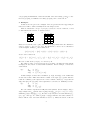
2. Examples
In this section we give some examples. All concepts and notation appearing in
this section will be defined formally in the following sections.
First we discuss the concept of grouping of relations. Let two relations, r1 and
r2 with schemas R1 and R2 , be as listed below.
r1 :
A
a1
a2
a3
r2 :
B
b1
b2
b3
B
b2
b2
b3
b4
C
c1
c2
c3
c4
D
d1
d2
d3
d4
First we note that R1 ∩ R2 = {B}, and that the (tuple) values in the B-columns are
πB (r1 ) ∪ πB (r2 ) = {[b1 ], [b2 ], [b3 ], [b4 ]}. We shall write r1 and r2 as a combination
of the B-tuples. Clearly, r1 can be written as
{[b1 ]} × {[a1 ]} ∪ {[b2 ]} × {[a2 ]} ∪ {[b3 ]} × {[a3 ]} ∪ {[b4 ]} × {}
and r2 can be written as
{[b1 ]} × {} ∪ {[b2 ]} × {[c1 , d1 ], [c2 , d2 ]} ∪ {[b3 ]} × {[c3 , d3 ]} ∪ {[b4 ]} × {[c4 , d4 ]}
We refer to this as the grouping of r1 and r2 by B.
We define a class of environments from a grouping. As usual an environment
is simply an association of values with identifiers. As an example, consider the
environment
η[b2 ] :
#
@(1)
@(2)
7→
7→
7
→
[b2 ]
{[a2 ]}
{[c1 , d1 ], [c2 , d2 ]}
In this example, we have three identifiers, #, @(1), and @(2), each of which has
an associated value. This environment consists of the tuple [b2 ] together with the
relations consisting of the tuples from r1 and r2 which contain [b2 ]; except that in
@(1) and @(2), the [b2 ]-parts of the tuples have been removed. Similarly, we have
η[b4 ] :
#
@(1)
@(2)
7→
7→
7→
[b4 ]
{}
{[c4 , d4 ]}
We can evaluate expressions in different environments. As an example, @(1) ×
@(2) evaluated in η[b2 ] (this is denoted [[@(1)×@(2)]]η[b2 ] ) is {[a2 , c1 , d1 ], [a2 , c2 , d2 ]}.
Similarly, [[@(1) × @(2)]]η[b4 ] = {}. Because of the way the four environments η[b1 ] ,
η[b2 ] , η[b3 ] , and η[b4 ] are defined, [[@(1) × @(2)]]η will have the same schema, no
matter which of the four environments we use for η. Thus, the union of all four
2
(partial) results is well-defined. The expression
group r1 , r2 by B do @(1) × @(2)
denotes exactly this value, {[a2 , c1 , d1 ], [a2 , c2 , d2 ], [a3 , c3 , d3 ]}. In fact, by this example, we have given an informal semantics of the grouping operator. In standard relational algebra, the relation just computed could have been expressed by
πX (r1 ✶ r2 ), where X = (R1 \ R2 ) ∪ (R2 \ R1 ).
We move on to an example using aggregation. We use the notation SUMA (r),
where r is a relation which has an integer attribute A. This expression evaluates to
the sum of the integers in column A of r.
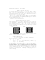
Consider the relation Sales with schema
{SalesPerson, District, Customer, Amount},
which contains information about sales by different salespersons, i.e., which salesperson, which district, to whom, and the total value of the sale. In the following,
we use the initial letters: S, D, C, and A. Also for brevity, let Jones denote
πDCA (σS=Jones (Sales)), and let Miller denote πDCA (σS=Miller (Sales)). We use the
following example data:
Jones:
D
2
7
7
7
8
C
Smith
Lee
O’Neil
Brown
Chang
Miller:
A
17
20
12
2
7
D
7
8
8
13
C
Clark
Morrison
Kent
Hansen
A
25
9
9
12
Now for each of the districts numbered from 5 through 20, we want to find the
difference of their sales. This can be expressed by
group Jones,Miller by D do
(5 ≤ D) ∧ (D ≤ 20)? {# [V : SUMA (@(1)) − SUMA (@(2))]}
A typical environment looks like this:
η:
#
@(1)
@(2)
7→
7→
7→
[D : 7]
{[C : Lee, A : 20], [C : O’Neil, A : 12], [C : Brown, A : 2]}
{[C : Clark, A : 25]}
For this environment, the boolean expression (5 ≤ D) ∧ (D ≤ 20) evaluates to
true. This means that we proceed to evaluate the expression following the question
mark. Had it evaluated to false, the result of the whole evaluation (for this particular
environment) would be the empty relation (with schema {D, V }). As it is, we obtain
a relation consisting of one tuple, which is the concatenation of [D : 7] (the value
of #) and [V : 9] (the value of [V : SUMA (@(1)) − SUMA (@(2))]). In total, we
obtain the following:
3
D
7
8
13
V
9
−11
−12
For each district, we can find the number of customers that Jones have dealt
with, but Miller has not as follows:
group Jones, Miller by D do {# [V : COUNTA (πC (@(1)) − πC (@(2)))]}
Of course, the minus here is relation difference.
New possibilities arise when nesting is allowed. Consider division, usually defined as:
r1 /r2 = {t | {t} × r2 ⊆ r1 }
We can write
group r1 , r2 by R2 do group @(1) by R1 \ R2 do {#} × r2 ⊆ r1 ? {#}
Here grouping is with respect to more than one attribute name (R2 and R1 \ R2
should of course really be written out as a sequence of attribute names). The first
grouping provides us with @(1)’s consisting of tuples from r1 with schema R1 \ R2 .
The second group runs through these tuples one by one and includes them in the
result if they pass the test. The second grouping is basically a forall-construction,
since we group on the entire schema of the (one) argument relation.
3. Notation
We use standard relational algebra and calculus as defined in the original paper 1
or in textbooks 11 . In this section we specify which variants we are using.
We fix a domain D of all constants that can appear in relations and expressions, and an infinite set A of attribute names. In this paper there is no reason to
distinguish between different types, so schemas are simply finite subsets of A.
We fix the letters we use as names for various entities:
• a, a1 , a2 , . . . ranges over D and expressions of that type.
• A, A1 , A2 , . . . , B, C range over A.
• X, Y range over finite subsets of A.
• t, t1 , t2 , . . . , u, x, x1 , x2 , . . . range over tuples.
• r, r1 , r2 , . . . , e, e1 , e2 , . . . range over relation names and expressions.
• R, R1 , R2 , . . . , E, E1 , E2 , . . . range over schemas of relations and expressions.
• c, c1 , c2 range over Boolean expressions (conditionals).
4
A tuple is a total function from a schema into D. We write t.A for t’s value
on the attribute name A. Constant tuples are listed using square brackets, so
[A1 : a1 , . . . Ak : ak ] is the tuple such that t.Ai = ai , 1 ≤ i ≤ k. The empty tuple
(the function defined on the empty schema), is written [ ].
A relation is a schema R and a finite set of tuples r. The schema of every tuple
t ∈ r must be R. The notation R(r) is used to indicate that relation r has schema
R. As usual, we sometimes overload notation and let r refer to the relation R(r).
We need a notation for empty relations with different schemas: if Z is a set of
attribute names (a schema), then we let Z(∅) denote the relation with schema Z,
but no tuples. Thus, ∅(∅) is the empty relation with the empty schema. There are
exactly two different relations with the empty schema, namely ∅(∅) and ∅({[ ]}) (the
latter is the neutral element with respect to Cartesian product and natural join).
If e is a relational expression, then we always let the corresponding capital letter,
E, denote the schema of the relation, the value of which the expression e denotes.
If t is a tuple, {t} denotes the corresponding singleton relation.
We use standard symbols for the relational operators: ∪, −, ×, σ, π, and δ for
union, difference, Cartesian product, selection, projection, and renaming, respectively. Select conditions consist of a single equality or inequality between two attribute names or an attribute name and a constant. If t = [A1 : a1 , . . . Ak : ak ] and
{A1 , . . . , Ak } ⊆ R, then we use σt (r) as short for σAk =ak (· · · σA2 =a2 (σA1 =a1 (r)) · · ·).
This could equivalently be written {t} ✶ r. We also use the derived operator natural
join, ✶ .
Finally, it will be convenient for us to allow projection on an empty set of
attribute names. The obvious generalization is that π∅ (r) is ∅(∅), if r is empty, and
∅({[ ]}), otherwise.
For relational calculus, we use a tuple-based variant.
The atomic formulas are t ∈ r, where r is a relation, as well as t.A θ t.B and
t.A θ a, where A and B are attribute names, a is a constant, and θ is one of <, >,
=, 6=, ≤, and ≥.
A formula is an atomic formula, or one of ¬p, p ∧ q, p ∨ q, ∃t : p or ∀t : p, where
p and q are formulas.
If X is a subset of the schema of some tuple t, then t[X] denotes the tuple t
restricted to X, i.e., its schema is X, and for every A ∈ X : t[X].A = t.A. As a
special case, t[∅] is the empty tuple.
A tuple relational query is an expression of the form {t | p}, where p is a formula,
and t is the only free variable in p. We use the convention that t is defined on any
attribute mentioned in connection with t in the query, e.g., if t.A and t[X] appears
in p, then t is defined on {A} ∪ X.
4. Relational Algebra with Grouping
To make the presentation clearer, we initially omit nested groupings and computations on domain values, including aggregation. In the last sections, we discuss
how these restrictions are removed. We define the extension of relational algebra
which is specified in Fig. 1 using BNF-notation.
5
<atom> ::= a | #.A
<tup> ::= [ ] | [A : <atom>] | #
<rel> ::= r | Z(∅) | {<tup>} | <cond>? <rel> | @(1) | @(2) | . . . |
<rel> ∪ <rel> | <rel> − <rel> | <rel> × <rel> |
σAθC (<rel>) | πA1 ...Ak (<rel>) | δA→B (<rel>)
<cond> ::= <atom> ≤ <atom> | <rel> ⊆ <rel> |
<cond> ∧ <cond> | <cond> ∨ <cond> | ¬<cond>
Figure 1: Grammar for the extended language.
<atom>, <tup>, <rel>, and <cond> stand for atomic expression, tuple expression,
relational expression, and conditional expression, respectively.
An atomic expression can be a constant or a tuple selection.
A tuple expression can be the empty tuple, a constant tuple, or a grouping tuple.
A relational expression can be a relation name, the empty relation with schema
Z, a singleton relation containing only the one specified tuple, a gate expression
(which evaluates to its relational argument if the condition evaluates to true), grouping relations, or a standard relational operator applied to relational expressions.
There is the additional syntactical restriction that # must appear in the scope
(in the do-part) of a grouping expression, and @(i) must appear in the scope of a
grouping expression with at least i arguments.
A conditional expression can be a comparison between domain values or relational values, or it can be a Boolean formula over conditional expression.
In order to focus on what is essential, we have left out unnecessary constructions.
For instance, all the usual six comparison operators can be expressed using ≤ and
the Boolean connectives. Similarly for containment of relations, ⊆.
Also, tuple concatenation has been used in the examples, but since the expression in the grouping construction must be relational, tuples can be converted
into singleton relations sooner, and Cartesian product can be used instead. For
instance, {# [R : SUMA (@(1)) − SUMA (@(2))]} from an earlier example can be
written {#} × {[R : SUMA (@(1)) − SUMA (@(2))]}.
Finally, in the examples, an attribute name A has denoted the value of the
current grouping tuple on A. In the grammar, we require that the explicit form
#.A is used instead.
For now, until we allowed nested applications of grouping, we discuss the language where we have only one grouping construct with a relational expression,
defined by the BNF-grammar, in the do-part:
group r1 , . . . , rn by A1 , . . . , Ak do <rel>
We require that every attribute Aj in the by-part appears in every schema Ri .
T
In other words, {A1 , . . . , Ak } ⊆ i Ri .
We now formally define the meaning of such an expression. We do this in terms
of the standard relational operators, but notice that this does not define a standard
6
relational algebra expression, since, among other things, we use a data dependent
number of unions. Compare with the first example in Section 2.
Definition 1 Let F = group r1 , . . . , rn by A1 , . . . , Ak do e, where
\
X = {A1 , . . . , Ak } ⊆
Ri
i
The semantics of F is denoted [[F]] and defined by
[
[[F]] =
[[e]]ηt
t∈bF
where bF =
S
i
πX (ri ), and for each t ∈ bF and i ∈ {1, . . . , n},
i,t
= πRi \X (σt (ri ))
rF
and, finally, for each t ∈ bF , we define the environment ηt by
ηt :
#
@(1)
..
.
7→
7→
..
.
1,t
rF
@(n)
7→
n,t
rF
t
..
.
Note that # is always bound to a tuple value with schema X, and @(i) is a
relation with schema Ri \ X.
5. Computational Power Is Preserved
We show how a grouping expression can be translated into relational calculus.
Since relational algebra and calculus are equivalent 2 , this shows that grouping
expressions can also be translated into relational algebra. Since the grouping expressions contain a complete 2 version of relational algebra, grouping expressions
are equivalent to relational algebra.
An expression group r1 , . . . , rn by A1 , . . . , Ak do e is translated into
_
{x | ∃t# :
(∃ti : ti ∈ ri ∧ ti [X] = t# ) ∧ T (e)}
i
where the translation of e, T (e), is defined in Fig. 2.
In that table, we use t# for values corresponding to #, and ti for tuples belonging
to the relation ri . Additionally, we use X for the set A1 , . . . , Ak , i.e., the schema of
t# (and #).
With regards to scope of variables, we assume that in each step of a recursive
translation, parenthesis are used around the entire formula in the right column of
the table. The scope of universal and existential quantification extends as far to
the right as it is meaningful, i.e., to the first unmatched right parenthesis.
Finally, we use the following convention in order to make the table readable.
The translation is compositional, so the translation of a composite expression is
7
given in terms of the translations of the components. Expressions are translated
into formulas with exactly one free variable. When a composite expression is to be
translated, we assume that the first expression is translated into a formula, where
the only free variable is x1 , and the second expression is translated into a formula,
where the only free variable is x2 . For the only free variable in the result, we use
the variable x. When translating a formula recursively, this means that after a
subexpression has been translated, the free variable, x, must be renamed to x1
(other occurrences of x1 should first be renamed to some new variable).
exp
T (exp)
Domain expressions
a
a
#.A
t# .A
Tuple expressions
[]
x = []
[A : a]
x.A = T (a)
#
x = t#
Relation expressions
ri
x ∈ ri
Z(∅)
false
{u}
T (u) ∧ x = x1
@(i)
∃ti : ti ∈ ri ∧ t# = ti [X] ∧ x = ti [Ri \ X]
c? e1
T (c) ∧ ∃x1 : T (e1 ) ∧ x = x1
e1 ∪ e2
(∃x1 : T (e1 ) ∧ x = x1 ) ∨ (∃x2 : T (e2 ) ∧ x = x2 )
e1 − e2
(∃x1 : T (e1 ) ∧ x = x1 ) ∧ ¬(∃x2 : T (e2 ) ∧ x = x2 )
e1 × e2
∃x1 : ∃x2 : T (e1 ) ∧ T (e2 ) ∧ x[E1 ] = x1 ∧ x[E2 ] = x2
σA θ a (e1 ) ∃x1 : T (e1 ) ∧ x = x1 ∧ x.A θ a
σAθB (e1 ) ∃x1 : T (e1 ) ∧ x = x1 ∧ x.A θ x.B
πY (e1 )
∃x1 : T (e1 ) ∧ x = x1 [Y ]
δA→B (e1 ) ∃x1 : T (e1 ) ∧ x = x1 [E1 \ {A}] ∧ x.B = x1 .A
Conditional expressions
a1 ≤ a2
T (a1 ) ≤ T (a2 )
e1 ⊆ e2
∀x1 : T (e1 ) ⇒ ∃x2 : T (e2 ) ∧ x1 = x2
c1 ∧ c2
T (c1 ) ∧ T (c2 )
c1 ∨ c2
T (c1 ) ∨ T (c2 )
¬c1
¬T (c1 )
Figure 2: Translation into relational calculus.
Example 1 Consider the following expression:
group r1 , r2 by R1 ∩ R2 do @(1) × @(2)
In relational algebra, this would be expressed as:
π(R1 ∪R2 )\(R1 ∩R2 ) (r1 ✶ r2 )
8
In both cases, the attributes on which to group or project would be given explicitly,
though. Let X be the set of attributes R1 ∩ R2 .
Changing variable names whenever necessary, the translation defined above results in:
W
{x | ∃t# :
i (∃ti : ti ∈ ri ∧ ti [X] = t# ) ∧
∃x1 : ∃x2 :
∃t1 : t1 ∈ r1 ∧ t# = t1 [X] ∧ x1 = t1 [R1 \ X]
∧ ∃t2 : t2 ∈ r2 ∧ t# = t2 [X] ∧ x2 = t2 [R2 \ X]
∧ x[R1 \ R2 ] = x1 ∧ x[R2 \ R1 ] = x2 }
We state the following result.
Theorem 1 For any sequence of relations, r1 , . . . , rn , any set of attribute names
T
X ⊆ i Ri , and any relation expression e,
_
[[group r1 , . . . , rn by X do e]] = {x | ∃t# :
(∃ti : ti ∈ ri ∧ ti [X] = t# ) ∧ T (e)}
i
W
Proof. Note that t# ∈ i πX (ri ) if and only if i (∃ti : ti ∈ ri ∧ ti [X] = t# ) is
true. Thus, the result can be established by showing that for all environments, ηt′ ,
S
where t′ ∈ i πX (ri ), we have that [[e]]ηt′ = {x | t# = t′ ∧ T (e)}.
This equality can be shown by an induction argument, by going through the
translations defined in Fig. 2. The proof is simple, but lengthy, and has been
omitted.
✷
S
6. Nested Groupings
In this section we briefly consider the necessary and desired additions when
nested groupings are allowed, and we give the extensions to the semantics and to
the translation into relational calculus.
First the BNF-grammar from Fig. 2 is extended with the following:
<rel> ::= group <rel>, . . . , <rel> by A1 , . . . , Ak do <rel> |
\@(1) | \@(2) | · · · | \\@(1) | \\@(2) | · · ·
<tup> ::= \# | \\# | · · ·
So now groupings can appear anywhere a relational expression is expected.
When a grouping is used in the do-part of another grouping, two sets of grouping tuples and grouping relations are active at a time. The intention is that # and
the @(i)’s refer to the nearest grouping and \# and the \@(i)’s refer to the grouping
one level further out. So we must require that if, for instance, \@(i) is used, then
the grouping one level out has at least i arguments. In general, the number of \’s
specifies the level relatively to the current.
As an example, consider the query
group r1 , r2 by Y do group @(2), r3 by Z do @(2) × \@(1)
where Y and Z are some sets of attribute names. Here the first @(2) comes from
r2 , the second @(2) comes from r3 , and \@(1) comes from r1 .
To be precise about the meaning of a nested query, we extend the definition
of the semantics of grouping. First, if η is an environment, then we let \η denote
9
the environment where all names have been equipped with an extra \, e.g., if η
was defined on the set of names {#, @(1), \#, \@(1), \@(2)}, then \η is defined on
{\#, \@(1), \\#, \\@(1), \\@(2)}. Assuming that η ′ and η ′′ are defined on disjoint
sets of names, we use η = η ′ ⊕η ′′ to denote the combination of the two environments,
where η is defined on the union of the two sets of names, and the value on a given
name is the value from either η ′ or η ′′ .
When extending Definition 1, the crucial change is that grouping can now appear in the expression e. Thus, we must be able to evaluate a grouping construction in an environment. Using the notation just defined, the semantics of
S
[[group r1 , . . . , rn by X do e]]η should be t∈bF [[e]](\η ⊕ ηt ).
When defining the translation of nested queries into relational calculus, we must
introduce a variable t′# for each nested grouping. This should be a new variable
name each time since we want it to be in the scope of the t# ’s defined at levels
further out. Translation of #’s preceded by a number of \’s, is then simply a
matter of using the correct t′# . Grouping relations are handled similarly.
7. Aggregation and Computation on Domain Values
We extend the BNF-grammar from Fig. 1 with the following:
<atom> ::= AGGRA (<rel>) | <atom> op <atom>
Thus, an atomic expression can now also be an aggregation of a given attribute
over a given relation. Here, AGGR could be any of the usual aggregate functions,
i.e., SUM, COUNT, MAXIMUM, etc. Furthermore, an atomic expression could be
some operation applied to other atomic expressions, e.g., one of the usual arithmetic
operations addition, subtraction, multiplication, or division.
Since we have seen how we can translate any relational expression into relational
calculus, we can also express the result of an aggregation, assuming that relational
calculus is extended with some appropriate construction for this 6 . We could use a
construction such as ∃tSUMA : p, where t is the only free variable in p. The value
of this expression is the sum of the t.A’s for all t which fulfill p.
The translation does not, in principle, become any harder. However, since relation expressions can now appear inside tuple expressions (via domain expressions),
we cannot just use a compositional translation as in Fig. 2. Instead, we have to define a separate analysis and translation of tuples. This is simple, but cumbersome,
and has been omitted.
Acknowledgments
The author would like to thank an anonymous referee for suggesting that the
translation of the extended relational algebra be made into relational calculus instead of into relational algebra.
References
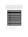
1. E. F. Codd, “A Relational Model of Data for Large Shared Data Bases”, Communications of the ACM, 13(6) (1970) 377–387.
10
2. E. F. Codd, “Relational Completeness of Data Base Sublanguages”, In: Data Base
Systems, Randall Rustin (ed.), 65–98 (Prentice-Hall, 1972).
3. Peter M. D. Gray, “The GROUP BY Operation in Relational Algebra”, In:
Databases, S. M. Deen, P. Hammersley (eds.), 84–98 (Pentech Press Limited, 1981).
4. Peter M. D. Gray, “Logic, Algebra and Databases”, (Ellis Horwood Limited, 1984).
5. G. Jaeschke, H. J. Schek, “Remarks on the Algebra on Non First Normal Form Relations”, In: Proceedings of the 1st ACM SIGACT-SIGMOD-SIGART Symposium
on Principles of Database Systems, 124–138 (ACM Press, 1982).
6. Anthony Klug, “Equivalence of Relational Algebra and Relational Calculus Query
Languages Having Aggregate Functions”, Journal of the ACM, 29(3) (1982) 699–
717.
7. Kim S. Larsen, “RASMUS User’s Manual”, MD-60, Computer Science Department,
Aarhus University, 1992.
8. Kim S. Larsen, Michael I. Schwartzbach, Erik M. Schmidt, “A New Formalism for
Relational Algebra”, Information Processing Letters, 41(3) (1992) 163–168.
9. Akifumi Makinouchi, “A Consideration on Normal Form of Not-NecessarilyNormalized Relations in the Relational Data Model”, In: Proceedings of the Third
International Conference on Very Large Data Bases, 447–453 (IEEE Computer Society Press, 1977).
10. Jan Paredaens, Dirk van Gucht, “Converting Nested Algebra Expressions into Flat
Algebra Expressions”, ACM Transactions on Database Systems, 17(1) (1992) 65–93.
11. J. D. Ullman, “Principles of Database and Knowledge-Base Systems, Vol. 1”, (Computer Science Press, 1988).
11