Download Chapter 7_Transient

7 Setting up and Execution of
Transient Simulations
.....
Chapter 7: Setting up and execution of transient simulations
7.1
7.2
7.3
7.4
Introduction..........................................................................................................................................7-3
Opening a transient data set................................................................................................................7-3
Transient options..................................................................................................................................7-4
Definition of transient parameters........................................................................................................7-5
7.4.1 Introduction..................................................................................................................................7-5
7.4.2 Definition by user defined stress inputs.......................................................................................7-6
7.4.3 Definition by time series allocation...............................................................................................7-7
7.4.4 Definition of precipitation excess from Fluzo...............................................................................7-9
7.5 Definition of a transient calibration file...............................................................................................7-10
7.6 Definition of a time series output file..................................................................................................7-10
7.7 Simulation options..............................................................................................................................7-11
7.8 Executing the transient simulation.....................................................................................................7-12
7.9 Viewing output results........................................................................................................................7-12
Royal Haskoning
Triwaco User's Manual
7.1 Introduction
Apart from steady-state simulations, Triwaco also allows the user to carry out time dependent or transient
model simulations. Transient simulations are based on data defined in one of the steady-state simulation
data sets, a 'Calibration' data set, a 'Scenario' data set or a 'Final' data set, and may even be based on
another 'Transient' data set. In addition to the steady-state parameters some additional parameters have to
be defined:
•
•
•
the effective porosity of the top-aquifer (PE), when phreatic;
the storage coefficient for each aquifer (SCi, with i = 1,,N);
the initial conditions for the groundwater head (HT and HHi, with i = 1,,N).
All steady-state parameters, inherited from another data set, may be replaced by time dependent or transient
parameter sets. For example, where the water level HR1 of the rivers is essentially constant in time for
steady-state calculations, it may in fact vary in time. In that case, the inherited parameter set is replaced by a
time dependent parameter set.
At the moment Transient simulations using ModFlow is not supported. To carry out Transient simulations
using ModFlow contact the Triwaco helpdesk. Depending on the need by users this option can be
incorperated in a custom made version.
7.2 Opening a transient data set
The 'Transient data set' is created similarly to the other data sets by selecting 'Add' from the 'Dataset' pulldown menu and 'Transient data' from the 'create new dataset' dialog window. As usual, the user is
prompted to provide a description, the sub-directory name and the (unsaturated zone) data set and grid this
'Transient data set' is based on. A transient data set can be based on: a 'Calibration', a 'Scenario' data set.
As soon as the user has confirmed the choices for the Transient data set, by pressing the
-button, the
Transient options window will appear. The window contains two tab-sheets: 'Transient options' and
'Calculation options'. The 'Transient options' tab-sheet is used for the definition of the calculation period and
the so-called 'stress input times'. The 'Calculation options' tab-sheet various 'simulation options' are set.
7 Setting up and Execution of Transient Simulations-3
Royal Haskoning
Triwaco User's Manual
7.3 Transient options
The tab-sheet, labeled 'Transient options', is used to define the simulation period (start and end date) as
well as the time step size used in the simulation.
Definition of the simulation period
The simulation period is defined by the following paramters:
The start and end times is defined in
'dd/mm/yyyy hh:mm' and can be
selected from the drop-box.
The resulting length of the calculation period is calculated and displayed in gray.
Selecting the -icon will display a
calendar, which enables the user to easily
select the starting or end date required,
scrolling back and forth with
and
.
Double clicking on the month or the year
results in a list of months or a ruler for
selecting the year. The hours and
minutes of start and end times can be
selected by using the hour rulers at the
right.
Definition of stress input times
The stress input defines the times at which new parameter data input may be defined and output data are
generated. The stress input times may be defined in two ways:
•
Stress input times are generated automatically
From the time step specified the program computes successive input times beginning at the calculation's
start time. The time step has to be given in days. If hourly values are required these should be entered as
a fraction of a day (e.g. 1/24 day = 0.042 day). If input is required for every decade (approximately 10-day
period), as is often the case for precipitation and evaporation data, the stress input should read 10.146
days, resulting in 36 stress periods per year.
7 Setting up and Execution of Transient Simulations-4
Royal Haskoning
•
Triwaco User's Manual
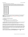
Stress input times are read from a so-called TIM-file
Choosing this option the user should specify name and location of the TIM-file to be used. This file
contains a series of dates and times, in the format specified before, that should be within the range
defined by the start and end time of the calculation. For each successive date and time the total time (in
days) since the start time is being computed. In example TIM stress input times file is given below.
After having defined the start and end time and the stress input times the user confirms his choice with the
-button. The 'Transient data set' is now added to the 'project window'. The 'Transient data
options window' may be reopened selecting 'Options' from the 'Transient' pull-down menu while the
Transient data set window is active.
7.4 Definition of transient parameters
7.4.1 Introduction
In the transient data set two types of allocation may be distinguished:
- allocation in space, which is the same as for steady-state calculations;
- allocation in time, needed for all time dependent input parameters.
For allocation in space the same allocators are used for parameter allocation within the other data sets (such
as Arpadi, InvDist, etc). Transient data set parameters for which allocation in space is sufficient are the
initial heads, the effective porosity and the storage coefficient for each aquifer.
In simulations where a phreatic aquifer is used Triwaco automatically decides when the effective porosity
(PE) or storage coefficient (SC1) for the uppermost aquifer applies. Where PHI1<RL1 (waterlevel <
groundlevel) PE is applies, when PHI1>RL1 SC1 applies. For all other layers a storage coefficient applies.
Because transient calculations need time dependent input, allocation in time is introduced here. (Allocation in
time will also be used in the 'Unsaturated data set, chapter 13'). Allocation in time and in space is combined
to generate transient parameter sets. For instance for the groundwater recharge time allocation is used to
produce 10-day values and allocation in space is carried out to interpolate between points and to generate
the distributed parameter sets.
In general the parameters displayed in the 'Modified parameters' tab-sheet are essentially time dependent
parameters, whereas the parameters from the 'Inherited parameters' tab-sheet are not time dependent.
Therefore, time allocation is carried out only for the 'modified' parameters.
7 Setting up and Execution of Transient Simulations-5
Royal Haskoning
Triwaco User's Manual
For the allocation and definition of the time dependent input parameters Triwaco uses two different methods:
- parameter input may be given at User defined stress inputs;
- parameter input may be defined by Time series allocation.
Selecting 'User defined stress inputs' the user can specify at which time steps changes in input parameters
will take effect (c.f. change in controlled water levels of polders). For the various ways of 'time series
allocation' a so-called TIM-file is needed. Time series allocation is introduced to be able to enter parameter
data, which are available in time series (c.f. meteorological data).
7.4.2 Definition by user defined stress inputs
At the left-hand side of the 'Time ruler window' the possible stress input times are presented as 'time
boxes'. Next to the time boxes the date, time and number of time step is given.
The tick-boxes in the time ruler can be checked . Whenever a box is checked the input parameter will be
loaded, during the transient calculation, at the corresponding time. The first time box is checked by default,
because most of the parameters are needed from the start of the calculation. If a parameter has to be used
for the whole calculation, it is not necessary to check all the time boxes; in fact this parameter is treated as a
steady-state input parameter. In this case it is sufficient to only check the first time box.
The groundwater flow simulation program reads parameters successively; once a parameter value is loaded
this value can only be changed overwriting it with a new set of parameter values, which will be done only at
input and output times mentioned in the input file. Hence, the parameter can not be switched off using the
'Time ruler'!
To be able to change parameter values using the 'Time ruler' a special parameter name is introduced,
consisting of the standard Triwaco parameter name followed by a '~' and a descriptive text string. The
groundwater flow program interprets the name as if only the part preceding the '~' existed.
For instance, changing abstracion rate or turning off an abstraction well can be accomplished by using the
following parameter names: 'SQ2~ON' and 'SQ2~OFF'.
The '~' in the parameter name causes the simulation program to neglect the remaining part, thus using the
parameter SQ2~ON' for the parameter SQ2 when it appears in the input file. Similarly, the program uses
'SQ2~OFF' if this parameter name is found in the flairs.fli input file. The values, however, are read from the
proper parameter files: RP5~on.ado and RP5~off.ado.
Thus, using the 'Time ruler' one can specify at which (input) times the parameter value should switch from
'SQ2~ON' to 'SQ2~OFF', vice versa. If the parameter 'SQ2~ON' is loaded at e.g. 01/01/1997, by checking the
appropriate time box, the parameter's values will be overwritten if the time box for 'SQ2~OFF' is checked at
12/03/1997 . Thus, wells in aquifer 2 are active (when defined in SQ~ON) from 01/01/1997 until 12/03/1997,
and well defined to be inactive (when defined in SQ2~OFF) from 12/03/1997 onwards.
Once the stress input times are defined in the 'Time ruler', the parameter can be allocated in the same way
as in the 'Calibration' or the 'Scenario' data sets. Using the option 'user defined stress inputs' thus results
in one single adore set for the parameter considered.
Transient parameters that do not change with time, like the effective porosity (PE), the storage coefficient
7 Setting up and Execution of Transient Simulations-6
Royal Haskoning
Triwaco User's Manual
(SC1, SC2 etc.) and the initial conditions (HT, HH1 etc.), can best be introduced using this option with the
first time box of the 'Time ruler' checked. For the definition of the initial conditions most often the calculation
results of a steady-state data set will be used. This is simply done using the expression allocator and
referring to the Result parameter in question. For example, if the initial conditions for the top-system have to
be read from the 'Calibration dataset' “calib1” one should define the parameter HT by the expression:
calib1$PHIT. See also chapter 5.1.5 for the definition of initial head parameters.
7.4.3 Definition by time series allocation
The 'Time series allocation' option is introduced to define input data given in a time series (e.g.
meteorological data, abstraction rates or surface water levels). Time series allocation is only possible for
those parameters displayed in the 'Modified parameters' tab-sheet.
The 'Time series allocation' type has to be activated at the right-hand side of the 'Time ruler' of a
parameter. Three types of 'Time series allocation' (TSA) are available:
TIM with parameter values
to be converted to intensities
TIM with parameter values
to be averaged
The input times in the TIM-file do not correspond with the stress input
times.
Parameter values are given as total for the successive time periods and
should be converted to an average intensity for the stress input time
period.
Example: precipitation values for a month, input required in daily values.
The input times in the TIM-file do not correspond with the stress input
times.
Parameter values are given for successive times or time periods and
should be converted to an average value for each stress input time period.
Example: Surface water levels at given times, input required a constant
level each stress input time
If one of the 'Time series allocation' types is switched on 'User defined stress input' is automatically
switched off and the stress-input list at the left-hand side of the 'Time ruler' window is disabled (graying it
out). There is no need to check the time boxes, because input is generated for every stress-input. The stressinput times are computed by the program from the start and end time and from the 'stress input in days'
defined in the 'Transient dataset options window' or read from the TIM-file specified
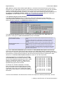
Transient parameters to be allocated with the 'Time
series allocation' option should be defined by a map
file and a time-dependent parameter file, the so-called
TIM-file. A TIM-file (with extension *.tim) has to be
generated by the user, which is easily done using a
spreadsheet program and a text editor.
An example of a TIM-file is displayed on the right.
Every set consists of the ID of the object in the map
file and a number of lines containing a date, time and
a parameter value. Every set is closed with the label
'END' and the total TIM-file is closed with an additional
label 'END'.
The time interval defined in the TIM-file does not have to be equal to the stress input time step. The time
7 Setting up and Execution of Transient Simulations-7
Royal Haskoning
Triwaco User's Manual
series allocator implemented in Triwaco interpolates between successive time intervals and adds input
values, if needed, to generate the proper values for each stress-input time step. The start and end of the
calculation, defined in the 'Transient dataset options window', should be within the range defined by the
first and last time of the TIM-file. Parameter values in the TIM-file should be given in the appropriate units
(e.g. monthly values of precipitation should be in meters). The output data sets, after time series allocation,
are given as intensity (e.g. precipitation intensity is computed in meters/day) or given in the same units as the
TIM-file, depending on the allocation type selected.
The TIM-file has to be defined in the 'Transient parameter information' window, which can be accessed
selecting 'Info' from the 'Parameter' pull-down menu. The TIM-file can be edited selecting 'View' 'TIM file'
from the 'Parameter' pull-down menu or 'View/Edit Tim File' from the parameter pop-up menu.
A time series parameter input file (or TIM-file) can easily be generated using a spreadsheet program (using
the MS Excel program one should use format: custom; dd/mm/yy hh:mm to properly format the date and time
columns). After the last 'END' the program expects a 'CARIAGE RETURN' or an 'ENTER'.
7 Setting up and Execution of Transient Simulations-8
Royal Haskoning
Triwaco User's Manual
As can be seen from the example TIM-file, a time series and corresponding parameter values should be
defined for each object in the map file (each having a unique ID). After 'Time series allocation' is selected
and the TIM-file is defined, allocation can be carried out.
All usual methods for allocation in space can be used in combination with the time series allocation. In fact
the TIM-file replaces the usual par file. Prior to the actual allocation, one can select 'Test Generate TSA file'.
An intermediate file is created in which the result of the conversion to average values or intensities for each
stress input time is given. Selecting 'Allocate' from the 'Parameter' pull-down or pop-up menu runs the actual
allocation program and the result is written to a file containing multiple adore sets. The parameter names of
the various adore sets consists of the 'usual' parameter name followed by the text string ",TIME=" and the
stress input time in days, relative to the start time of the calculation. Thus, the first adore set is labeled
"par,TIME= 0.00", with for par the standard Triwaco parameter name.
Note that if any one of the start or end time of calculation or the stress input period is changed (in the
'Transient dataset options window') all time dependent parameters in the 'Modified parameters' tabsheet have to be allocated again.
7.4.4 Definition of precipitation excess from Fluzo
For Transient simulations often time-dependent groundwater recharge is required. The module FLUZO
(explained in more detail in chapter 12, not yet available) simulates groundwater flow in the unsatureted zone
and determines the effective groundwater recharge. The effective groundwater recharge is one of the
parameters of the topsystem. The effective groundwater recharge is written to a file named fluzo.fzo. The
parameter RP1 is used to define the effective groundwater recharge in the Transient data set.
The transient groundwater recharge has to be defined in the 'Transient parameter information' window,
which can be accessed selecting 'Info' from the 'Parameter' pull-down menu. The fluzo result file fluzo.fzo has
a the standard adore file format. Select fluzo.fzo from the Fluzo directory (search for *.fzo). The definition of
RP1.ung, RP1.par can be neglected. Next activate the 'Time series allocation' type 'TIM with parameter
values to be converted to intensities' at the right-hand side of the 'Time ruler'. There is no need to allocate
this parameter since the resulting groundwater recharge is already in the appropiate adore format (fluzo.fzofile). To prevent from accidental allocation select None as allocator.
It is important to realise that the simulation period (start and end-date) as well as the timestep size have to be
identical for both the Fluzo simulation and for the Transient simulation.
7 Setting up and Execution of Transient Simulations-9
Royal Haskoning
Triwaco User's Manual
7.5 Definition of a transient calibration file
If a calibration file (calib.chi) is present, Triwaco automatically compares calculated hydraulic heads with
the data from observation wells. After comparison Triwaco will calculate the average deviation, the average
absolute deviation, the squared average deviation, the minimum deviation and the maximum deviation. To
view or edit the calibration file select 'Calibration'|'Calibration'|'View/Create Input' from the pull down menu.
The input file has a fixed format described in chapter 10. The output of the calibration can be viewed as table
('Calibration'|'Calibration'|'View Output') or as a background map in Triplot ('Calibration'|'Calibration'|View
Map'). A comprehensive description on the usage of the calibration (calib.chi) file is given in chapter 10.
7.6 Definition of a time series output file
Time series of simulated groundwater heads for user defined locations, defined by its coordinates, may be
optained by defining a graphnode input file. The resulting graphnode output file is a comma delimited file and
can be imported in a standard spreadsheet program to generate time graphs of groundwater heads. For all
locations after each successive iteration step calculated results are written to the output file.
The graphnode input file is defined in the Transient options window under the Calculation options tabsheet. The graphnode input file is defined as a standard Triwaco map file, i.e. ungenerated graphnode.ung
file, by which user defined points are defined (see below) or a calib.chi file as used in a steady state
simulation.
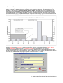
The output file contains a short descriptive heading of four records, the title for each output parameter and a
series of records with the values for the output parameters. The example shown below gives the output for
one user defined location for a model with one aquifers (A01). The values for the (phreatic) head in the topsystem is found in the column for A00. Example Time series output file: Graphnode.out
To generate time series for an arbitrary result parameter, transient simulation result or time dependent input
parameter an auxiliary program is available (mikado). The program reads a standard Triwaco calibration file
(calib.chi, for a steady-state thus without the time of observation) and the flairs.flo output file and creates an
output file with, for each output time, the parameter name (e.g. "PHI1,TIME: 10.0000") followed by the
calculated parameter values at the location of the observation wells.
7 Setting up and Execution of Transient Simulations-10
Royal Haskoning
Triwaco User's Manual
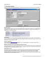
7.7 Simulation options
The sheet, labeled 'Calculation parameters', displays the parameters for the definition of the calculation
scheme:
Iteration options
In this section the number of inner and outer iterations are set, as well as the criterion for convergence and
the value for the relaxation factor. These parameters may be adopted from steady-state calculations in a
'Calibration' or 'Scenario dataset'.
Description
Inner iteration
Outer iteration
Function
Sets the maximum number of inner iterations
Sets the maximum number of outer iterations
Convergence
Sets the criterion for convergence
Relaxation
Sets the relaxation factor
Print options
In this section the user may specify the parameters that will be written to the output file. For each layer the
desired output has to be checked
. By default all output parameters will be printed. Output is placed in the
flairs.flo file using the Adore format.
Points for time lines
In this section the graphnode input file is defined. The use and application is explained in the previous
section paragraph 7.6.
Maximum allowed change in groundwater head per time step
This parameter defines the way simulation program determines the iteration time step size. The default value
for this parameter is set to 0.25 m. However, in case of strongly varying surface water levels (during a flood)
one might choose to increase this value to e.g. 5 m.
Initial time step size
The initial time step size is used by the simulation program every time new (time dependent) data is read.
The default value for this parameter is set to 0.1 day. However, in case of a strongly varying situation
(temporary abstraction from wells) one might choose to decrease this value to ensure a more stable
calculation process. This however is not a necessity since the simulation program will automatically choose
the best value during the simulation process.
7 Setting up and Execution of Transient Simulations-11
Royal Haskoning
Triwaco User's Manual
Effective porosity vs storage coefficient
In simulations where a phreatic aquifer is used Triwaco automatically decides when the effective porosity
(PE) or storage coefficient (SC1) for the uppermost aquifer applies. Where PHI1<RL1 (waterlevel <
groundlevel) PE is applies, when PHI1>RL1 SC1 applies. For all other layers a storage coefficient applies.
7.8 Executing the transient simulation
Selecting 'Generate input' from the 'Transient' pull-down menu will create the main input file for transient
groundwater flow calculations. This file has by default the name flairs.fli. The file differs from the steadystate input files by different calculation flags in the second line of the input file. Moreover, at the end of the
input file a number of records are added to define the stress-input and the corresponding time dependent
parameters for the transient calculations. A complete overview of the flairs.fli input file is given in chapter 5.
Selecting 'Run simulation' from the 'Transient' pull-down menu will start the transient groundwater flow
computations.
After termination of the computations, the results may be viewed graphically using TriPlot. The calculation
process and the results are summarised in the output files: flairs.flg, flairs.flp and flairs.flo described in
chapter 5.2.6
All output is gathered in one and the same flairs.flo output file, and no 'Result parameters' tab-sheet will
appear. Output is only generated at the stress-input times for which input data is defined. If a user wants to
create more output times, one and the same parameter must be loaded at the desired times.
7.9 Viewing output results
Selecting 'View' 'Results' from the Calibration pull down menu starts the graphical presentation program
TriPlot, loads the grid information and displays the layout of the model area. Alternatively, the user can select
one of the parameters from the 'result parameters' sheet and viewing the parameter separately selecting
'View' 'Adore' from the Parameter pull down menu or 'View Adore file' from the pop-up menu (right hand
mouse button). Adding other parameters (selecting 'Param' 'Load' from theTriPlot menu bar) gives the user
7 Setting up and Execution of Transient Simulations-12
Royal Haskoning
Triwaco User's Manual
the opportunity to compare result parameters with model input parameters.
Contouring or classifying transient results is similar to that of a steady state simulation result. Creating an
animation from contoured or classified results is explained in chapter 9. Creating time series graphs for any
transient parameter is also explained in chapter 9.
7 Setting up and Execution of Transient Simulations-13