1
Residential New Construction (RNC)
Programs Impact Evaluation
Appendices to Volume I.
California Investor-Owned Utilities’ Residential New
Construction Program Evaluation for Program Years 20062008
Study ID: CPU0030.02
Final Evaluation Report - Prepared by:
KEMA, Inc.
The Cadmus Group, Inc.
Itron, Inc.
Nexus Market Research, Inc.
Prepared for:
California Public Utilities Commission – Energy Division
February 8, 2010
Experience you can trust
Experience you can trust
Appendices
Table of Contents
A.
B.
Calculation of Adjusted Tracking Savings Estimates......................................................... A-1
A.1 Orientation Adjustments ........................................................................................... A-1
A.2 Ratio Estimation and B-Ratios.................................................................................. A-1
A.3 Summary of Results ................................................................................................. A-2
A.4 Interpretation and Conclusions................................................................................. A-2
A.5 Single Family Adjusted Gross Energy Savings ........................................................ A-3
Residential New Construction Onsite Data Collection ....................................................... B-1
B.1 Building Characteristics ............................................................................................ B-1
B.2
Performance Testing ................................................................................................ B-7
B.2.1 Whole House Infiltration................................................................................ B-7
B.2.2 Total Duct Leakage Protocol ...................................................................... B-13
B.3 End Use Meter Data Collection .............................................................................. B-17
B.3.1 Cooling Equipment End Use Metering........................................................ B-17
B.3.2 Domestic Hot Water End Use Metering...................................................... B-21
B.3.3 Heating Equipment End Use Metering ....................................................... B-26
C. End Use Meter Data Analysis ............................................................................................ C-1
C.1 End Use Equipment Meter Data............................................................................... C-1
C.1.1 Cooling Equipment ....................................................................................... C-1
C.1.2 Water Heating Equipment............................................................................. C-4
C.1.3 Space Heating End Use Energy ................................................................... C-5
C.2 Data Summary.......................................................................................................... C-6
D. Net Savings: Difference-of-Differences Calculation Methodology and Comparison
Groupings .......................................................................................................................... D-1
D.1 Methodology and Equations for Computing Net Savings ......................................... D-1
E. The RNC Interface ............................................................................................................. E-1
E.1
E.2
F.
Introduction............................................................................................................... E-1
Overview of the RNC Interface................................................................................. E-1
E.2.1 MICROPAS Version 4.5, 5.1, 6.0, 6.5, 7.0, and 7.3 ..................................... E-2
E.2.2 Developing MICROPAS Inputs from the On-Site Survey Data..................... E-2
E.2.3 Features of the RNC Interface...................................................................... E-3
E.3 Testing the RNC Interface ........................................................................................ E-4
Baseline Study Results .......................................................................................................F-1
F.1 Newly Built Single Family Homes over Time.............................................................F-4
California Public Utilities Commission
i
February 8, 2010
Appendices
Table of Contents
F.2 Fenestration Baseline Results...................................................................................F-6
F.3 Space Heating Systems Baseline Results ................................................................F-8
F.4 Space Cooling System Baseline Results ..................................................................F-9
F.5 Multiple HVAC Systems and Thermostat Types Baseline Results..........................F-10
F.6 Water Heating Baseline Results..............................................................................F-11
F.7 Percent Duct Leakage Baseline Results .................................................................F-13
G. Verification-Guided Programs............................................................................................ G-1
G.1 California Multifamily New Homes – Net to Gross Results...................................... G-1
H.
I.
J.
K.
L.
California Multifamily New Homes Net-to-Gross Interview Guide...................................... H-1
Designed for Comfort Onsite Inspection Forms...................................................................I-1
California Multifamily New Homes Detail Tables ................................................................ J-1
Baseline Study and RNC Evaluation Recruitment Details ................................................. K-1
Public Comments on the Draft Evaluation Report with Responses ....................................L-1
List of Exhibits:
Figure B-1: Installation of Blower Door Frame.......................................................................... B-8
Figure B-2: Placement of Green Pressure Tubing.................................................................... B-9
Figure B-3: Installation of Blower Door Fan .............................................................................. B-9
Figure B-4: Attach the Fan to the Cross Bar........................................................................... B-10
Figure B-5: Attach Pressure Gauge........................................................................................ B-10
Figure B-6: Attaching the Pressure Tubing to the Pressure Gauge........................................ B-11
Figure B-7: Connecting Power to the Blower Door Fan.......................................................... B-12
Figure B-8: Fan Direction Switch ............................................................................................ B-12
Figure B-9: Installing the Duct Blaster .................................................................................... B-14
Figure B-10: Connecting the Pressure Tubing to the Pressure Gauge................................... B-15
Figure B-11: Placing Static Pressure Probe in Supply Register ............................................. B-15
Figure B-12: Connect Red Pressure Tube to Duct Blaster Fan .............................................. B-16
Figure B-13: Connect Controller to Duct Blaster Fan ............................................................. B-16
Figure B-14: Onset 0-50A CTV-B Current Transducer ........................................................... B-18
Figure B-15: Hobo U12-006 4-Channel External Logger........................................................ B-18
Figure B-16: Owl 400 Data Logger ......................................................................................... B-20
Figure B-17: Circuit Details ..................................................................................................... B-22
California Public Utilities Commission
ii
February 8, 2010
Appendices
Table of Contents
Figure B-18: Domestic Hot Water Data Logger Installation .................................................... B-23
Figure B-19: G4 Gas Sub-Meter ............................................................................................. B-25
Figure B-20: Typical Logger Installation for Forced Air Furnaces........................................... B-27
Figure B-21: Typical Switch Diagram...................................................................................... B-29
Figure F-1: Single Family Homes Built in California since 1998 ............................................... F-5
Figure F-2: Percentage of SF Homes with 2-paned Vinyl, Low-E Windows ............................. F-8
Figure F-3: AFUE Distribution – Average Statewide................................................................. F-9
Figure F-4: SEER Distribution – Average Statewide .............................................................. F-10
Figure F-5: Multiple HVAC System – Statewide Average ....................................................... F-11
Figure F-6: Percentage of Instantaneous Water Heaters (Gas and Electric).......................... F-12
Figure F-7: Homes with More than One Water-Heating Unit .................................................. F-12
Figure F-8: Percentage of Homes with Radiant Barriers ........................................................ F-13
Table A-1: B-ratios for Orientation Adjustments ....................................................................... A-2
Table A-2: Single Family Tracking Savings and Orientation Adjusted Savings ........................ A-3
Table B-1: Testo 327-1 Combustion Analyzer Specifications ................................................. B-28
Table C-1: Single Family Metering Summary ........................................................................... C-6
Table F-1: California Single Family Home Construction and Participation ............................... F-5
Table F-2: Percent Glazing ....................................................................................................... F-6
Table F-3: Distribution of Window Types – Detached Single Family Homes............................ F-7
Table F-4: Central Gas Space Heating System Efficiency ....................................................... F-8
Table F-5: Average SEER ........................................................................................................ F-9
Table F-6: Average Percent Duct Leakage............................................................................. F-14
Table F-7:................................................................................................................................ F-14
Table G-1: Performance Track Net to Gross Values for Each Project......................................G-1
Table G-2: Appliance Track Net-to-Gross Values for Each Project ..........................................G-2
Table J-1: Performance Track Net to Gross Values for Each Project........................................J-1
Table J-2: Performance Track Net to Gross Values for Each Project........................................J-2
Table J-3: Appliance Track Net-to-Gross Values for Each Project ............................................J-1
Table K-1: RNC Site Recruitment Sample Disposition ............................................................. K-2
Table L-1: Comments on the Draft Report with Responses ......................................................L-1
California Public Utilities Commission
iii
February 8, 2010
Appendices
A.
Calculation of Adjusted Tracking Savings
Estimates
A.1
Orientation Adjustments
Orientation adjustments were only necessary for homes recorded in the CalCERTS registry.
The orientation of a home can significantly affect its space cooling and heating energy
requirements, chiefly due to solar gain through windows. However, when RNC participating
homes are built and entered into the tracking registries (CHEERS and CalCERTS) their actual
orientations are not recorded. Instead, production builders design homes which are built in all
possible orientations, usually dependent upon the layout of the streets in a development. To
accommodate this style of planning and to satisfy the RNC program requirements, builders
model their homes in north, east, south, and west orientations to show that energy consumption
meets minimum program requirements in all four “cardinal” orientations. The CHEERS registry
contains the modeled energy consumption for all four orientations, and the average was used to
calculate the gross energy savings for each home.
The CalCERTS registry only contains modeled energy for each plans’ worst orientation, but
clearly not all homes are actually built in the worst possible orientation. To adjust for this, the
CHEERS data were used to estimate “average” orientation energy as a function of worst
orientation energy. Unique orientation adjustment b-ratios were estimated for the single family
homes.
A.2
Ratio Estimation and B-Ratios
Ratio estimation was used to adjust gross tracking energy savings through the use of b-ratios in
six stratum: three end uses (heating, cooling, and water heating) in each of three climate
regions (inland, coastal and high desert).1 The target variable of analysis, denoted y, is the
energy use of the project (home). The primary stratification variable, the estimated energy
savings of the project, is denoted x, and is obtained from the tracking database. A ratio model
1
A home was classified as either coastal, desert or inland based on its CEC climate zone. Homes modeled (or built)
in CEC climate zones 1-7 were classified as coastal, homes in CEC climate zone 15 was classified as desert, and
homes modeled in CEC climate zones 8-14 and 16 were classified as inland.
California Public Utilities Commission
A-1
February 8, 2010
Appendices
was formulated to describe the relationship between y and x for all projects in the population,
such that y = βx. In statistical jargon, the ratio model is a (usually) heteroscedastic regression
model with zero intercept. Beta (β) is referred to as a b-ratio. In the case of orientation
adjustment, β is the sum of all homes’ average orientation energy savings divided by the sum all
homes’ worst orientation energy savings within a stratum. A thorough description of ratio
estimation can be found in the 2004 California Evaluation Framework. 2
The orientation adjustments are based on a sample size of over 5,500 single family homes from
the CHEERS registry.
A.3
Summary of Results
Orientation adjustment results are presented in Table A-1.
Table A-1: B-ratios for Orientation Adjustments
Climate
Region
Coastal
Desert
Inland
Heating
Cooling
1.11
1.16
1.14
1.28
1.06
1.29
B-ratios less than one indicate less energy savings than computed from the tracking data, while
b-ratios greater than one yield increased savings. All of the B-ratios were greater then one
implying that the worst orientation reports less savings then the average orientations used in the
CHEERS registry.
A.4
Interpretation and Conclusions
These findings, although not the focus of this report, are very significant. For example, the
orientation results show that inland energy savings can be increased by 29% for space cooling,
and 14% for space heating, by orienting a home from its worst energy orientation to its average
2
TecMarket Works, 2004. The California Evaluation Framework. Prepared for the California Public Utilities
Commission and the Project Advisory Group
California Public Utilities Commission
A-2
February 8, 2010
Appendices
energy orientation. 3 Even greater energy savings could be achieved by orienting homes to
their best orientation or by selecting designs specific to the orientation of the site. This is not a
“new” discovery, as the advantages of passive solar design and home orientation have been
known for centuries, but the orientation adjustment b-ratios, based on analysis of thousands of
homes, provide a quantitative estimate of the energy “cost” to builders of ignoring orientation.
Conversely, water heating orientation b-ratios are 1.0, since the orientation of a home does not
impact modeled energy water heating usage.
A.5
Single Family Adjusted Gross Energy Savings
B-ratios were multiplied by gross savings from CalCERTS tracking data to arrive at the
Orientation Adjusted Tracking Savings.
The overall impact of the orientation adjustment on gross tracking savings is presented in Table
A-2. Gross tracking savings from the raw data (for which savings estimates could be obtained)
increases by 6.42% as a result of the adjustment. We multiplied the CalCERTS portion of gross
savings by the b-ratios for orientation adjustments to arrive at the orientation adjusted gross
savings.
Table A-2: Single Family Tracking Savings and Orientation Adjusted Savings
Utility
PG&E
SCE
SCG
Total
Single
Family
Dwelling
Units
5,244
414
67
5,725
Tracking before
orientation
adjustment
(source kBtu)
87,816,143
7,513,120
1,455,735
96,784,998
Tracking after
orientation
adjustment
(source kBtu)
93,393,552
8,146,578
1,455,735
102,995,866
%
change
6.35%
8.43%
0.00%
6.42%
Note that the percent change was zero for SCG . This is because all of SCG participants were
on the CHEERS database and no adjustments were needed.
3
Although coastal space cooling savings increases by a dramatic 28% with orientation adjustment, the actual energy
savings due to this adjustment are small since the coastal region has much smaller cooling loads and many fewer
new homes.
California Public Utilities Commission
A-3
February 8, 2010
Appendices
B.
Residential New Construction Onsite Data
Collection
B.1
Building Characteristics
Data collection for each site includes information on the building’s characteristics, HVAC
equipment serving the home, lighting, and major appliances per the IOU’s prescriptive
measures. This data will be used to inform Micropas input files. The details of these input
parameters are described below.
For a given residential site, modeling parameters fall into the following hierarchy.
1) Site Overview Information
a) Overall floor area
b) Number of floors
c) Type of residence (single family, attached, etc)
d) Vintage of Residence
e) Number of bedrooms/bathrooms
f)
City (CIMIS weather data)
g) Utility Meters and Accounts
h) Title 24 Documents if available
i)
Builder/Development Information
j)
Age and Number of Residents
k) Number of residents home during the day time
2) HVAC and Ventilation Systems
a) Primary Heating and Cooling Systems
California Public Utilities Commission
B-1
February 8, 2010
Appendices
i)
System type (central, room unit, hydronic, etc.)
ii) Equipment type (split, packaged, heat pump, furnace, baseboard, etc.)
iii) Manufacturer
iv) Model number (Indoor and Outdoor for split systems)
v) Cooling capacity
vi) Cooling efficiency (SEER and EER)
vii) TXV (thermostatic expansion valve) or non-TXV
viii) Refrigerant Type (R-22, R-410a)
ix) Heating capacity (kBtuh)
x) Heating efficiency (AFUE, HSPF, or COP)
xi) Evaporative cooling
xii) Supply fan type (CV, two-speed, ECM, VSD)
xiii) Presence of whole house fan, Smart Vent/Economizer, mechanical
ventilation
xiv) Indoor fan motor HP if available
b) HVAC Schedules (for each system)
i)
Thermostat Manufacturer/Type
ii) Thermostat Model Number
iii) Thermostat set points for heating and cooling during occupied and
unoccupied periods
c) Duct Systems
i)
Location of Ducts
ii) Location of Registers
California Public Utilities Commission
B-2
February 8, 2010
Appendices
iii) Duct Types
iv) Duct Sealant Types
v) Insulation R-Value
vi) Duct and Plenum Condition
vii) Total duct leakage (duct blaster test)
3) Envelope Characteristics
a) Exterior Walls
i)
Exterior wall construction Type
ii) Surface Type
iii) R-value
iv) Orientation (N, S, E, W)
v) Shading
vi) Number and Type of Doors
vii) Wall Area
b) Windows
i)
Number of panes
ii) Glass type (clear, tinted, reflective, LowE (using EKT detector))
iii) Frame type (metal, vinyl, wood)
iv) Frame Style (fixed, slider, etc)
v) Height and width of each window
vi) Quantity of each type
vii) Internal/External Shading
California Public Utilities Commission
B-3
February 8, 2010
Appendices
viii) Orientation
c) Interior Walls
i)
Height and width
d) Roofs
i)
1. Type
ii) 2. Surface area
iii) 3. Surface (Tile, Shingle, etc)
iv) 4. Color
v) 5. Ceiling insulation R-value or type
e) Floors
i)
Number of Floors
ii) Total Conditioned Floor Area
(1) Ground Floor Area
iii) Construction Type (slab, crawl space, open)
iv) Area of Exposed Slab or perimeter
v) Area Over Unconditioned Garage
vi) Raised floor R-Value if available
4) Lighting
a) Interior Lighting (to be catalogued in Title 24 spaces defined by usage)
The following parameters will be collected for all interior lights:
i)
Fixture type
ii) Fixture wattage
California Public Utilities Commission
B-4
February 8, 2010
Appendices
iii) Lamps per fixture
iv) Lamp wattage
v) Mounting type (recessed, direct, indirect, direct-indirect, track, plug in
task, or furniture integrated task)
vi) Control strategy (switch, dimmer, occupancy sensor, etc.)
b) Exterior Lighting
The following parameters will be collected for all exterior lights:
i)
Fixture type
ii) Fixture wattage
iii) Control strategy
5) Appliances and Other Equipment
a) Hot Water Heaters
i)
Type (storage, instantaneous, heat pump)
ii) Manufacturer
iii) Model number
iv) Tank capacity
v) Input [kBtuh gas, kW electric]
vi) Fuel type
vii) Location
viii) Insulation Jacket
ix) Insulation on pipes
x) Presence of hot water reclaim
xi) Efficiency, %
California Public Utilities Commission
B-5
February 8, 2010
Appendices
xii) Low flow fixtures
xiii) Temperature settings (low, medium, high)
xiv) Recirculation control type and pump HP
b) Refrigerators and Freezers
i)
Manufacturer
ii) Model Number
iii) Configuration (top mount freezer, side-by-side, etc)
iv) Location (conditioned, unconditioned space)
v) Volume
vi) Age
vii) Energy Star
viii) Presence of through-the-door water or ice
ix) Automatic ice maker
x) Energy Factor (ft3/kWh/day)
c) Dishwasher
i)
Manufacturer
ii) Model Number
iii) Energy Star
iv) Builder Installed, Purchased New, Installed Used
d) Clothes Washer/Dryer
i)
Manufacturer
ii) Model Number
California Public Utilities Commission
B-6
February 8, 2010
Appendices
iii) Energy Star
iv) Builder Installed, Purchased New, Installed Used
v) Axis Type/Fuel Type
e) Oven, Range, Pool/Spa Heater
i)
f)
Fuel Type
Pool Pump
i)
HP
ii) Speed
g) Number of televisions and size, and number of computers
h) Number of non-lamped ceiling fans and location
B.2
Performance Testing
B.2.1
Whole House Infiltration
To measure the infiltration of a home we used the Minneapolis blower door ™. The Minneapolis
blower door ™ uses a fan and frame assembly that is temporarily sealed into an exterior
doorway. The testing was performed at a pressure difference of 50 Pa (0.2 inches of water
column) to create a slight pressure difference between the inside of the home and outside.
Using a digital pressure gauge to measure the air flow that is required to maintain 50 Pa, the air
tightness of the house can be gauged.
B.2.1.1
Setup Procedure for Blower Door Test
1) Close all windows and doors to the outside.
2) Open all interior doors and supply registers.
3) Close all dampers and doors on wood stoves and fireplaces. Seal fireplace or
woodstove as necessary to prevent ash blowback into occupied spaces.
4) Make certain furnace and water heater cannot come on during test.
California Public Utilities Commission
B-7
February 8, 2010
Appendices
5) Put water heater and/or gas fireplace on “pilot” setting if they are within the
conditioned space.
6) Make certain all exhaust fans and clothes dryer are off.
7) Make certain any other combustion appliances will not be backdrafted by the
blower door.
8) Make certain doors to interior furnace cabinets are closed.
9) Also make certain crawlspace hatch is on, even if it is an outside access.
10) Check attic hatch position.
11) Put garage door in normal position.
12) If dryer is not installed seal off dryer vent.
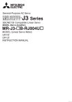
Performing Blower Door Test Setup
1) Setup and install Blower door frame in an exterior doorway- do not put fan in
opening yet (see Figure B-1).
Figure B-1: Installation of Blower Door Frame
California Public Utilities Commission
B-8
February 8, 2010
Appendices
2) Put the Green pressure tubing through one of the opening in the door, run it
approximately 3-5 feet away making sure that the end of the tubing is placed well
away from the exhaust flow of the Blower Door fan (see Figure B-2).
Figure B-2: Placement of Green Pressure Tubing
3) Install the Blower door fan in the opening making certain the elastic band fits
snuggly around the fan with the collar resting in between the two sides of the
electrical box (see Figure B-3).
Figure B-3: Installation of Blower Door Fan
California Public Utilities Commission
B-9
February 8, 2010
Appendices
4) Attach the fan to the cross bar with the Velcro strap- the fan should now be
suspended in the door with the flow plate side facing towards you (see Figure
B-4).
Figure B-4: Attach the Fan to the Cross Bar
5) Attach pressure gauge to mounting board and put on gauge hanger (see Figure
B-5).
Figure B-5: Attach Pressure Gauge
6) Connect the Red pressure tubing to the Channel B Input Tap and connect the
other end to the pressure tap located on the blower door fan (see Figure B-6).
California Public Utilities Commission
B-10
February 8, 2010
Appendices
7) Connect the Green pressure tubing to the Channel A Reference Tap (see
Figure B-6).
Figure B-6: Attaching the Pressure Tubing to the Pressure Gauge
California Public Utilities Commission
B-11
February 8, 2010
Appendices
8) Insert plug into blower door fan and connect to power supply-Make certain the
fan speed controller is off when connecting to power (see Figure B-7).
Figure B-7: Connecting Power to the Blower Door Fan
9) Make certain fan direction switch is positioned towards the direction of airflow
(see Figure B-8. Connecting power to the blower door fan
Figure B-8: Fan Direction Switch
10) Perform Blower Door Test.
B.2.1.2
Blower Door Depressurization Test Procedures Using the DG-700
1) Press the Mode button twice for PR/FL@50.
2) If BD3 is not displayed on Channel A push Device until BD3 is displayed.
3) Push Configure button to select a flow ring displayed on Channel B. Typically
you should start with ring B2 (Open= No Ring A1= ring A, B1= ring B) the rings
on the blower door fan are labeled as such.
California Public Utilities Commission
B-12
February 8, 2010
Appendices
4) If you cannot get an accurate flow you will need to add or remove flow rings
on the blower door fan as well as change the Config for the appropriate ring. If
LO appears in the Channel B window it means that the gauge cannot
accurately calculate and a different flow ring should be used.
5) Turn on Fan and increase the fan speed until you get a pressure reading on
Channel A between -45 and -55 Pa. The gauge when in PR/FL@50 mode
will automatically adjust, so don’t worry about getting exactly to 50 Pa.
6) Once you have reached a pressure that is acceptable press the Hold button.
7) Record the BD ring used, House pressure near -50Pa on Channel A and
the BD CFM@50 value on Channel B.
8) Press HOLD Button again to release and PRESS MODE button to PR/PR and
record BD FAN PRESSURE value from CHANNEL B.
9) Repeat test at 25Pa and QC using the flow exponent equation (make sure to
set the Mode to PR/FL@25).
10) If Flow exponent checks out no further tests are required.
To check test, calculate the flow exponent, n. Use the following formula, n =
ln(Q50/Q25)/ln(P50/P25). Note Q50 and Q25 are the flows through the blower door at the testing
pressures (which are denoted P50 and P25. Depending on the test, you may not get the house to
exactly –50 or –25 Pa WRT outside. Use the exact ∆P you measure when checking the flow
exponent. For example, if the house gets to –48 Pa for the high ∆P, use this as the P50 in the
equation. If the flow exponent is not between 0.50 and 0.75, repeat the test.
Note testing conditions (if windy, inaccessible room(s), garage door open or closed, etc).
B.2.2
Total Duct Leakage Protocol
To measure the HVAC system duct leakage, a Minneapolis Duct Blaster® was used. The
Minneapolis Duct Blaster® measures the amount of leakage in the duct system by pressurizing
the ducts with a calibrated fan and simultaneously measuring the air flow through the fan. The
duct blaster fan is connected directly to the duct system in a house, typically at a central return,
or at the air handler cabinet. The remaining registers and grilles are taped off. The duct system
is then pressurized to 25 Pa and duct system leakage is measured using a digital pressure
California Public Utilities Commission
B-13
February 8, 2010
Appendices
gauge. The test is done in order to measure total duct leakage, which includes leakage inside
the thermal envelope of the home.
B.2.2.1
Setup Procedure for Total Duct Pressurization Test
1) Make sure HVAC is turned off and blower compartment door is in place.
•
Remove all air filters.
•
Tape all registers. Use appropriate tape (Long Mask) for friable surfaces.
Performing Total Duct Pressurization Test Setup
1) Install the duct blaster at the duct system at the central return or air handler
cabinet (the return will be the most common installation; see Figure B-9). In the
case of multiply returns seal off the smaller return and use the largest return for
test.
Figure B-9: Installing the Duct Blaster
2) Connect the Green pressure tubing to the Input tap on Channel A and the Red
pressure tubing to the Input tap on Channel B (see Figure B-10).
California Public Utilities Commission
B-14
February 8, 2010
Appendices
Figure B-10: Connecting the Pressure Tubing to the Pressure Gauge
3) Connect the other end of the Green pressure tube to the static pressure probe
and insert probe into a supply register and re-tape to secure probe in place
(see Figure B-11).
Figure B-11: Placing Static Pressure Probe in Supply Register
4) Connect the other end of the Red pressure tube to the duct blaster fan (see
Figure B-12).
California Public Utilities Commission
B-15
February 8, 2010
Appendices
Figure B-12: Connect Red Pressure Tube to Duct Blaster Fan
5) Next connect the controller to the duct blaster fan by the female power receptacle
and plug into power supply (see Figure B-13). Make certain fan controller is
off when connecting to power.
Figure B-13: Connect Controller to Duct Blaster Fan
6) Perform Duct Leakage Test.
B.2.2.2
Total Duct Pressurization Test Procedures Using the DG700
1) Turn on Duct blaster Fan and Pressure Gauge
2) Push Mode button to PR/FL
3) Push the Device button until DB B is displayed on the Channel A side
California Public Utilities Commission
B-16
February 8, 2010
Appendices
4) Next push the Config button to select a flow ring (Open= no ring,A1=ring 1,
B2=ring 2,C3=ring 3)
5) Adjust duct blaster fan speed control until Channel A reads 25 PA or as close
as possible
6) Record values
7) Repeat steps 1-6 with duct blaster test pressure of 50 PA
8) Record values and check flow exponent.
9) If flow exponent is within range test is complete.
10) Note any unusual testing conditions (wind, etc.):
11) If flow exponent is within range test is complete.
12) Note any unusual testing conditions (wind, etc.):
To check each test, calculate flow exponent as for the blower door test (previous page). The
flow exponent, n, = ln(Q50/Q25)/ln(P50/P25). If flow exponent not between 0.50 and 0.75, repeat
test.
B.3
End Use Meter Data Collection
This plan entails equipment monitoring at the primary residence(s) for the following equipment
comprising the three Title 24 end-uses over the course of one year:
1) Central and wall air conditioning units
2) Domestic hot water heaters and boilers
3) Central and wall heating systems
B.3.1
Cooling Equipment End Use Metering
1) Data points to be metered
a) Time series current logging of the unit
California Public Utilities Commission
B-17
February 8, 2010
Appendices
2) Monitoring equipment to be used
a) Hobo U12-006 4-channel logger with appropriate
Or
b) Owl 400 with appropriate CT for current monitoring
3) Sampling interval and Duration of metering
a) Loggers are typically set at 15 or 20 minute sampling interval
b) Duration of metering is for a full year
4) Hobo U12-006 Logger and Associated Sensors (see Figure B-14. Onset 050A CTV-B Current Transducer
Figure B-14: Onset 0-50A CTV-B Current Transducer
Figure B-15: Hobo U12-006 4-Channel External Logger
California Public Utilities Commission
B-18
February 8, 2010
Appendices
Data Logger Properties
•
U12 4-External Channel Logger accepts a wide range of external sensors,
including temperature, AC current, AC voltage, CO2, 4-20mA, and 0-2.5
VDC. 12-bit resolution provides great data accuracy.
•
One channel will be used for real-time amp monitoring of the AC unit
Installation Procedure
•
Connect the CT to channel 1 of the logger.
•
Open up the CT, and slip in the CT in one leg of the HVAC unit. Select the
leg that includes supply/condenser fan
•
Logger will launch using delay launch settings set in the office before bringing
to the field
5) OWL 400 Data Logger
Data Logger Properties
•
These loggers combine with a 50A current transducer to measure AC current.
•
To setup the Owl 400 data logger you must have ACR trend reader software
installed and running on your computer.
•
Used in conjunction with either Hobo Micro Station or Hobo Temperature
loggers.
California Public Utilities Commission
B-19
February 8, 2010
Appendices
Figure B-16: Owl 400 Data Logger
Installation Procedure
1) First, make sure that the secondary end of the Sentran current transducer is
plugged into the data port of OWL400.
2) Open up the split core CT, and slip in the CT in one leg of the HVAC unit. Select
the leg that includes supply/condenser fan
3) Logger will launch using delay launch settings set in the office before bringing to
the field
Additionally, one-time hand recorded field measurements will be collected for the following:
1) Air conditioner condenser unit amps
2) Air conditioner power factor
3) Premise voltage
Spot power reading and ambient air temperature (from weather station) measurements will be
taken while on site. Two spot power measurements will be taken, and the average of the two
will be used in the analysis.
California Public Utilities Commission
B-20
February 8, 2010
Appendices
The amperage draw of each central air conditioning condenser unit will logged at the electrical
disconnect and will be representative of all power consumed for wall units and the split-system
outdoor components including compressor, condenser fan, and controls.
For split systems, this amperage data in conjunction with the instantaneous readings of the
unit’s voltage and power factor along with nameplate fan power draw are used to calculate
kilowatt and kilowatt hour energy use for cooling. If multiple air conditioning units are found at a
site, all units will be summed together to produce the measure of total unit usage.
B.3.2
Domestic Hot Water End Use Metering
B.3.2.1
Gas Storage DHW
A storage tank heater maintains a set volume of hot water at a specified temperature at all times
regardless of need. It operates by releasing hot water from the top of the tank when a hot water
tap is turned on. To replace that hot water, cold water enters at the bottom of the tank, ensuring
that the tank is always full. A thermostat monitors the water temperature and enables the
burner to fire when the temperature drops below a pre-defined set point.
Installing an inline gas meter to precisely measure the annual gas consumption of water heaters
would not have been cost effective. An economical and accurate way to measure the gas
consumption is to record annual runtime of the burner. The temperature of the water heater flue
is an indicator that the burner is firing; therefore, we logged the temperature of the exhaust flue
to give the number of fires and duration of each firing of the hot water burner. We developed an
approach to measure the temperature of the exhaust flue with help of a negative temperature
coefficient (NTC) thermistor that provides a reliable and consistent indicator of burner run time.
Hobo Micro Station along with a 0 – 5 Volt adapter and a voltage divider was used to monitor
the temperature of the exhaust flue of the water heater. The voltage divider (bridge circuit) was
used to determine the resistance of the G type 10 K ohm @ 25°C NTC thermistor (Rt). The
balance resistor used with this bridge circuit is a fixed precision 2.2k ohm resistor (Rb). One end
of the thermistor was connected to the ground terminal of the Onset 0-5 Volt Adapter and the
other end was connected to the voltage input terminal of the adapter. One end of the balance
resistor was connected to the Trig. Source terminal of the volt adapter. Trig. Source provides
voltage from the logger’s battery to power the bridge circuit. The other end of the voltage
adapter was connected to a Hobo Micro Station logger. The details of the circuit are shown in
Figure B-17 below.
California Public Utilities Commission
B-21
February 8, 2010
Appendices
Figure B-17: Circuit Details
The HOBO Micro Station logger’s excitation voltage (Vexc) is the "switched DC output" coming
from the logger. Vexc provides 1 mA current at 2.5 volt DC. The 1 mA current flows through the
resistors to provide voltage across the bridge circuit. The voltage output from our bridge circuit
as seen by the logger input is (Vout). Thermistor to balance resistor ratio is Rt / Rb = Vout /
(Vexc-Vout). Now multiply the value of our Balance resistor (Rb) by this ratio to get the
resistance of the thermistor (Rt). To derive temperature from thermistor resistance plug values
into the Steinhart-Hart equation. The Steinhart and Hart equation is an empirical expression that
is used to determine the resistance temperature relationship of NTC thermistors. An Excel
spreadsheet developed by the vendor named 'Thermistor-hotplate' can be used to convert
voltage recorded by your Onset HOBO logger into temperature.
Field Installation
1) Drill a 3 /8” hole on the exhaust flue of the hot water and insert the 2” threaded
end of the thermistor into the flue and cover it with metal tape to secure the
thermistor for the duration of the study. Make sure the thermistor is in the
exhaust air stream and not making contact with the sides of the flue.
2) Insert PC interface cable to the communication port of the Hobo Micro Station to
configure the logger.
3) Follow the step-by-step process to setup the logger
a) Open the Hobo pro status window by double clicking the task bar or the
logger icon
California Public Utilities Commission
B-22
February 8, 2010
Appendices
b) Once status menu is displayed select launch logger option from device menu
c) Set the sample monitoring interval to 90 seconds
d) Then select launch options such as instant start, delayed start or push button
e) To start the logging session select the launch button
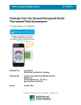
4) The HOBO Micro Station data loggers record an instantaneous flue temperature
every ninety seconds. The ninety second logging configuration permits 350 days
of monitored data. The loggers are configured to stop recording data when the
memory reaches capacity to avoid overwriting previously collected data. Figure
B-18 shows the typical logger installation implemented for storage domestic hot
water heaters with a standard flue.
5) Record the name plate information of the hot water heater such as make, model
number, serial number and nominal input (Btuh),
Note that the manifold (main burner) pressure will be measured on several units during the pilot
sites to verify proper delivery pressure.
Figure B-18: Domestic Hot Water Data Logger Installation
California Public Utilities Commission
B-23
February 8, 2010
Appendices
Data Processing
The recorded voltage data from the logger shall be downloaded to a PC. The voltage data is
converted into temperature with the help of 'Thermistor-hotplate' Excel spreadsheet for further
analysis.
B.3.2.2
Tankless Water Heaters
Instantaneous (tankless) water heaters operate without storage tanks. Cold water travels
through a pipe into the unit, and either a gas burner or an electric element heats the water only
when needed. As there are multiple controls to regulate the gas flow to the burner and the flow
is variable, the most economical and accurate way to measure the annual gas consumption is to
install an inline gas sub meter at the gas supply pipe of the water heater.
We used Elster Amco G4 gas meters to measure the annual gas consumption of the water
heater. This meter's small size and lightweight design is ideally suited for sub metering
applications. The G4 is a 200 cubic foot per hour, non-temperature compensated gas meter
with a cyclometer register. Despite its small size, the G4 is accurate and reliable when
measuring either natural or LP gas.
The design of the G4 consists of four measuring chambers separated by synthetic diaphragms.
The chambers are filled and emptied periodically and the movement of the diaphragm is
transferred via a gear to the crankshaft. This shaft moves valves that measure the volumetric
gas flow. Rotations of the gear are transferred via a magnetic coupling to the index, thus
assuring proper sealing of the meter’s internal mechanisms. Figure B-19 shows the G4 gas
meter.
California Public Utilities Commission
B-24
February 8, 2010
Appendices
Figure B-19: G4 Gas Sub-Meter
Field Installation
Authorized plumbers were hired to install the gas meter on the water heater. All gas safety
codes and regulations will abide by all terms and conditions imposed by the utilities and
governmental authorities.
1) Turn off the gas service to the house and cut the gas pipe before it enters the
tankless water heater.
2) Blowout the gas service line before the meter is installed, so that no dirt, debris
or liquids of any kind can be carried into the meter when gas is flowing through
the pipe.
3) Place a new connection washer on each open end of the gas pipe
4) Support the meter so that both hubs are against the connection washers and run
the connection nuts down hand tight.
5) In alternating fashion, tighten the nuts to an appropriate torque for the connection
size.
6) Before turning the gas on in a new installation, check the system downstream of
the meter to be sure that all connections are made up and tight or that the
downstream valve, if there is one, is closed.
7) Now reset the gas meter’s odometer and make sure that it reads zero.
California Public Utilities Commission
B-25
February 8, 2010
Appendices
8) Note down the date and time of installation
9) Record the nameplate information of the hot water heater such as make, model
number, serial number and nominal input (Btuh).
10) At the end of the monitoring period, record the cubic feet on the meter and also
the date and time of retrieval.
B.3.3
Heating Equipment End Use Metering
B.3.3.1
Forced Air Furnace
Heating systems monitored may include central forced air furnaces and central heat pumps.
Owl 400 data loggers are used for heat pump heating mode, and Owl 200 data loggers are used
for forced air furnaces. Considering the safety concerns and difficulty of measuring natural gas
consumption, a unique approach is necessary to capture the forced air furnace run-time. Inside
the air handler section of each furnace there is a low voltage (24 VAC) control board with a
terminal block consisting of separate relay contacts for heating, cooling, and fan operation.
Upon receiving a call for heat signal from the thermostat, the heating relay contact undergoes a
change of state resulting in the operation of the furnace. KEMA determined that by “slaving” a
small relay off of the call for heating circuit, and logging the change of state of the heating relay
contact, we were able to precisely log the percentage run-time of the furnace on an hourly
basis.
The furnace nominal input Btuh was obtained from the manufacturers’ specifications and utilized
to inform the run-time data with actual gas input. During the pilot sites the main burner gas
pressure was tested at each furnace unit to verify that the gas supply pressure was within the
manufacturer’s specifications. By doing this, we demonstrated that the gas supply pressure is
sufficient and RLW can confidently use the nameplate input Btuh rating for the fuel consumption
calculations.
Field Installation
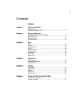
Figure B-20 below shows the typical logger installation implemented for forced air furnaces. For
two stage heating units, we installed a second relay and OWL 200 to capture run-time for each
stage.
California Public Utilities Commission
B-26
February 8, 2010
Appendices
Figure B-20: Typical Logger Installation for Forced Air Furnaces
90+AFUE Forced Air Furnace
Method A- Additional Measurements
Measurement of furnace inlet gas flow can performed during both high and low burn stages.
This could then be used to compute approximate gas usage.
Using the flue gas analysis kit, the combustion efficiency will be analyzed to ensure that the
furnace is operating near its rated efficiency. This is not equivalent to an AFUE rating. The flue
gas analysis kit determines O2, CO, probe temp., draft, and diff. pressure then calculates CO2,
CO-Air Free and Combustion Efficiency. The Testo 327-1 Combustion Analyzer specifications
are presented in Table B-1.
California Public Utilities Commission
B-27
February 8, 2010
Appendices
Table B-1: Testo 327-1 Combustion Analyzer Specifications
Parameter
Range
Resolution
O2
0 – 21%
0.1%
CO
0 – 4,000 ppm
1 ppm
Probe temp.
-40°F to +932°F
0.1°F
Draft
±16" H2O
0.001" H2O
Diff. pressure
±80" H2O
0.01" H2O
CO2
(Calculated)
0 – CO2 max
0.01%
In addition to the gas flow meter and flue gas analyzer, a relay and insulation piercing connector
was attached to the gas fuel value to measure the gas flow time (Flame-on). The flame on-times
was then compared with the times of the call-on events as recorded by the existing installed
meter. The difference between these two times under various firing regimes (e.g. the CPU
determined firing rate associated with prior short vs. long calls for heat) can be used to reduce
the furnace operating time as recorded over the entire metering period.
While the lag time for many furnaces has been published, our experience has shown that actual
lag times can vary substantially from published values. On average, the lag times were 144% of
published values, but they were as long as 183% for one furnace. The variation in lag time will
make it difficult to convert runtimes to gas use rates. One work-around is to use the average
observed value. This value varies from 9 second less to 23 seconds greater. For an average
cycle time of about 7 minutes, the error induced would be up to 5%, but would be lower in most
cases. While the improved observations of lag would improve the overall calculation, a greater
source of uncertainty relates to the CPU-controlled firing of stages.
There is significant uncertainty around the duration and frequency of low fire and high fire
events from two stage units. The determination of the cycle and the shift from low fire to high
fire, in some cases, is controlled by proprietary algorithms programmed into the furnaces control
circuitry. While the theory is relatively consistent – the programmed logic “learns” the demands
of the space and will respond consistently to calls from the thermostat based on the past calls –
a precise reproducible model appears to be unachievable, and despite numerous attempts, we
have been unable to gain access to the proprietary algorithms from manufacturers.
One way in which it might be possible to check the operational delay of low versus high output
modes is to modify the DIP switches in accordance with the furnace owners manual. See
Figure B-21 below for a typical switch diagram. In two-stage mode, this particular furnace will
California Public Utilities Commission
B-28
February 8, 2010
Appendices
have a 1-12 minute delay which will vary based on previous usage. The other DIP option will
produce a 5 minute delay between low and high firing modes regardless of previous usage.
Unfortunately, this solution will not work for all makes and models. The lack of a clear resolution
to this issue is why KEMA focused its efforts on a Method B as described below.
Figure B-21: Typical Switch Diagram
Method B- DOE Calculations
ASHRAE Standard 103 describes a methodology to determine a single stage equivalency for
modulating and 2-stage furnaces which will allow different models to be analyzed together. For
this method we first investigated if all the variables were available to determine estimated
consumption and low/high stage runtimes. Such variables include; ratio of blower on-time to
average burner on-time, fraction of heating load at reduced fuel input rate operating mode,
annual household heating load, and blower motor electrical power consumption.
California Public Utilities Commission
B-29
February 8, 2010
Appendices
According to resources from EERE, DOE calculated the gas consumed by the burner and
electricity consumed by the circulating air blower motor at the two firing rates. This calculation
method is based on the procedure in the ASHRAE Standard 103.
Summaries of the methodology are available at the following sites.
Uniform Test Method for Measuring the Energy Consumption of Furnaces:
http://www.fire.nist.gov/bfrlpubs/build02/PDF/b02022.pdf
http://www1.eere.energy.gov/buildings/appliance_standards/residential/pdfs/furnaces_boilers/fur
nace_boiler_app7_7.pdf
http://www1.eere.energy.gov/buildings/appliance_standards/residential/pdfs/furnrbod.pdf
http://edocket.access.gpo.gov/cfr_2009/janqtr/pdf/10cfr430BAppN.pdf
Using the equations and explanations available above and also through ASHRAE Standard
103, the AFUE of the furnace can be calculated. This procedure will also allow calculation of
the estimated gas usage of the furnace on an annual basis, which can be found by dividing the
annual household heating load by the AFUE and converting from BTUs to therms.
California Public Utilities Commission
B-30
February 8, 2010
Appendices
C.
End Use Meter Data Analysis
C.1
End Use Equipment Meter Data
C.1.1
Cooling Equipment
C.1.1.1
Split System Air Conditioner and Heat Pump
•
AC monitoring relies on data loggers recording average amperage every 20 minutes
using current transducers. The current draw data are combined with an instantaneous
power measurement (spot-watt) taken at the time of the meter installation.
•
It is then possible to translate these current readings into estimates of annual energy
consumption (kWh) of the air conditioner or heat pump.
•
Fan kWh is estimated by estimating the fraction of each period that the AC is running
and multiplying it by the kW input of the fan. To inform the run-time data with actual
power demand, a onetime spot power measurement of the condensing unit is taken
using a Fluke 31 power meter.
The air conditioner monitoring approach is to record total condenser run-time utilizing the OWL
400 data logger with a 0-2.5 vdc output 50 amp split core current transducer (CT). This
monitoring configuration operates by converting the analog signal of the 50 amp CT to a digital
signal usable by the OWL 400.
Energy consumption of blower fans for central cooling systems will not be metered explicitly, but
the fan is assumed to draw constant power during any condenser run period. The runtime for
air conditioning and heat pump systems will then multiplied by the fan power draw to determine
fan energy consumption. Cooling runtime for air conditioner and heat pump systems will
calculate using the data and equipment performance curves.
Cooling Runtime was calculated as follows:
1) First translate the measured amperage information into an estimate of runtime.
AMP = Average Amp data, 20-minute interval (OWL Data)
odb = condenser inlet dry bulb temperature (°F) (Hourly Data)
California Public Utilities Commission
C-1
February 8, 2010
Appendices
ewb = evaporator inlet wet bulb temperature (°F) (Assumed constant at 67 F)
2) Use the DOE-2 Bi-Quadratic performance curves for split systems.
Tonnage = nominal system capacity in tons (Based on nameplate and matching)
Cap = (nominal cooling capacity)= 12000•Tonnage (Btuh)
EER = System efficiency at standard conditions (Based on nameplate and
matching)
[The EER for each system was determined from the ARI Database of system
efficiencies based on the particular condenser and coil match. If no match could
be found the average EER for that SEER level across all manufacturers was
used. The EER is the amount of cooling delivered in kBtu/h divided by the power
input in kW at the standard condition of 95 F odb, and 67 F ewb.]
EIRARI = 3.412• (1/EER)
3) The bi-quadratic performance curves for cooling delivered and energy input ratio
as functions of condenser entering dry-bulb temperature (odb) and evaporator
entering wet bulb temperature (ewb) are presented below.
⎡1.191422708− 0.01965• (ewb ) + 0.000315625• (ewb ) 2
⎤
SysCool = Cap × ⎢
⎥
2
⎢⎣+ 0.0030587499• (odb ) − 0.00000933333 • (odb ) − 0.00007824999 • (ewb ) • (odb )⎥⎦
⎡- 0.06818927+ 0.0222843749 • (ewb ) - 0.00011718749 • (ewb )²
⎤
SysEIR = EIRARI× ⎢
⎥ ⎣+ 0.001059333 • (odb ) + 0.000148166 • (odb )² − 0.0002099999 • (ewb ) • (odb )]⎦
4) The results were then translated into power draw by multiplying the energy input
ratio by the amount of cooling delivered and converting the units back to Watts
from Btu/h. The equation below incorporates the unit conversion in the
determination power draw.
POWER=0.29308324•SYSEIR•SYSCOOL (Watts)
The power expected for a particular system with known efficiency and cooling
capacity at any given hour for a particular location is now known.
California Public Utilities Commission
C-2
February 8, 2010
Appendices
5) By combining the spot measurements taken at the time of meter installation, we
can then calculate the expected amperage draw given the local weather
conditions.
V = Volts from Spot Watt Data
PF = Power Factor from Spot Watt Data
AMPA=POWER / (V * PF)
6) If the unit was running for only a portion of the 20 minute interval the average
amps divided by the expected amps will yield the percentage of the interval the
unit was running at full power. Multiplying the percentage by one-third of an hour
(20 minutes) [or ¼, if at 15-min intervals] allowed for runtimes to be calculated in
units of hours. The equation below will be used for this analysis.
RUNTIME20 = (AMP/AMPA) * (1/3) (Hours)
7) The system’s energy consumption can then be calculated as the measure energy
consumption plus the fan energy consumption. The fan kW draw is assumed
constant and will be taken from nameplate data. The equations below show how
energy is computed using measured time series amperage data and
instantaneous power factor and voltage data along with computed runtime and
nameplate fan power.
FANKW = Fan Power for the system from nameplate data
ENERGY = (1/3) * AMP * PF * V + RUNTIME20 * FANKW
Heat Pump Separation Methodology
There were only six heat pumps installed at the 454 homes that were visited. None of these
homes were selected for metering, and therefore no Heat Pump methodology was used in this
analysis.
Filling in values for missing dates: Meter Data on Air Conditioners
For the meters that were collected before a full year had passed between the time of
installation, a method for filling in the missing data to create an annual usage profile was
California Public Utilities Commission
C-3
February 8, 2010
Appendices
needed. In light of this, weather normalization techniques were developed for the cooling end
uses to fill in the missing data for loggers with less than a year of recorded usage.
To calculate a year of data, a regression analysis was done based on the average daily
temperature and daily kWh. Cooling Degree Days (CDD) were calculated using the reference
temperature of 65 degrees F, and were used in the regression against kWh. Daily total usage
for the missing data was estimated using the equation below where β0 and β1 are constants
based on the regression analysis: β0 is the average daily baseline usage and β1 is the
temperature response of temperature-dependant cooling usage.
Daily Total Usage SITE = β0 + β1 *CDD.
The predicted Average Daily Usages were combined with the actual Average Daily Usage to
create a full year of daily usage for each site. For the meter adjustment factor estimation, these
daily usages were aggregated into annual kWh.
C.1.2
Water Heating Equipment
C.1.2.1
Storage Tank Domestic Hot Water (DHW) Heater
Temperature Cutoff Methodology (DHW heater). The voltage readings from the DHW loggers
were converted into temperatures using the following equation:
Temperature(C ) = (1/(0.001126733 + (log(2200 * (VDC/(2.5 - VDC)))) * 0.000234594) +
(0.0000000850781 * (log(2200 * (VDC/(2.5 - VDC)))) 3 + - 273.15 ))
The Temperature values were converted to Fahrenheit from Celsius and after a careful
examination of the Temperature profiles converted from the logger data, a cut-point of 185 8F
was established to differentiate between the on and off periods.
From the estimated on and off periods, an hourly percent runtime was calculated for each
heater. For the adjustment factor analysis, these hourly usage totals will be summed for the
8760 hours following the meter installation date to yield an annual total usage for the study
period. For sites that had less than a year of data, the usage was extrapolated to estimate the
annual usage. It was determined that the seasonal
California Public Utilities Commission
C-4
February 8, 2010
Appendices
C.1.2.2
Instantaneous Non Storage Domestic Hot Water (DHW) Heater
The G4 gas meter provided the total cubic feet gas consumed per year. We multiplied the total
cubic feet of natural gas by 1,020 to obtain total gas consumption of the water heater during the
installation period. This usage was then extrapolated based on the installation period and the
removal date to get an annualized estimate of gas consumption
C.1.3
Space Heating End Use Energy
C.1.3.1
Forced Air Furnace
The gas input and fan power draw was taken from nameplate data and applied to the unit
runtime to determine energy consumption. By “slaving” a small relay off of the call for heating
circuit we were able to precisely log the duration of a heating cycle. The relay contact change of
state indicates runtimes.
The final stored data was percent time “on” during each 20 minute interval. The furnace
nominal gas input rate (Btu/h) was obtained from the manufacturers’ specifications and utilized
to inform the run-time data with actual gas input. The runtimes were multiplied by the input
rating to estimate hourly gas consumption.
Filling in values for missing dates: Meter Data on Furnaces
A handful of meters were collected before a full year had passed between the time of
installation. For the purposes of the analysis, a full year of metered data was required in order
to create an accurate comparison with the modeled usages. In light of this, weather
normalization techniques were developed for the heating and cooling end uses to fill in the
missing data for loggers with less than a year of recorded usage.
To calculate a year of data, a regression analysis was done based on the average daily
temperature and daily kBtu. Heating Degree Days (HDD) were calculated using the reference
temperature of 65 degrees F, and were used in the regression against kBtu. Daily total usage
for the missing data was estimated using the equation below or similar form thereof where β0
and β1 are constants based on the regression analysis: β0 is the average daily baseline usage
and β1 is the temperature response of temperature-dependant heating usage.
Daily Total Usage SITE = β0 + β1 *HDD.
California Public Utilities Commission
C-5
February 8, 2010
Appendices
The predicted Average Daily Usages were combined with the actual Average Daily Usage to
create a full year of daily usage for each site. For the meter adjustment factor estimation, these
daily usages were aggregated into annual kBtu heating usages for the 365 days following the
meter installation date.
C.1.3.2
Heat Pump
There were no Heat Pumps in the meter data sample, so no methodology was developed or
used.
C.1.3.3
Hydronic Heating System
The data analysis developed a methodology to determine if hot water usage was attributed to
the space heating or domestic hot water end uses.
Hydronic Separation Methodology:
Note: Only one site was identified as having a hydronic heating system. Additionally, there was
an issue with the site data that failed to pass the QC standards set for the analysis.
Subsequently, the site was dropped.
C.2
Data Summary
The actual number of each type of system and the status and quality of the data obtained are
described in the following tables. As mentioned previously, single family homes used the same
metering approach for the three end uses at every site. Table C-1 below describes the number
of installed loggers for each end use and the status of the data obtained.
Table C-1: Single Family Metering Summary
Installed/ Bad/
Used in
Unit Type Retrived
Missing Analysis
142
20
122
AC
96
7
89
Furnace
57
0
57
DHW
There were a few reasons that sites were removed from the end use analysis. A handful of
loggers appeared to contain corrupt or incorrect data. A few appeared to be improperly installed
or configured. Another QC measure was based on the system tracking data. If a site appeared
to contain multiple units (AC or Furnace), but there were fewer loggers than systems, the entire
California Public Utilities Commission
C-6
February 8, 2010
Appendices
site had to be removed in order to ensure that the level of usage in the metered data was
consistent with the estimated model usage. It should be noted that the necessity of removing a
site from one of the end use analyses does not require that the site be removed from all the end
uses analyses. Each end use was analyzed separately, so bad data from one end use did not
affect the integrity of the other end use analyses.
California Public Utilities Commission
C-7
February 8, 2010
Appendices
D.
Net Savings: Difference-of-Differences Calculation
Methodology and Comparison Groupings
D.1
Methodology and Equations for Computing Net Savings
The essence of the “difference-of-differences” analysis is to compare participant homes to nonparticipant homes’ standard construction practices. While gross savings is defined as the
difference between standard (package D) and proposed modeled energy consumption, net
savings is defined as the gross savings less naturally occurring savings (due to industry
standard practice). If for one home,
Sp4 = Participant CF-1R standard energy use (kBTU/sf-yr)
Pp = Participant CF-1R proposed energy use (kBTU/sf-yr)
Snp = Non-participant CF-1R standard energy use (kBTU/sf-yr)
Pnp = Non-participant CF-1R proposed energy use (kBTU/sf-yr)
SF = Conditioned floor area of the home
Then, the
Net Savings = (Gross savings) – (Natural savings) = (Sp-Pp)*SF – (Snp-Pnp)*SF,
And the equation can be seen to motivate the name, as the net savings is indeed a
difference-of-differences.
(Snp–Pnp)*SF represents “the naturally occurring non-participant energy savings due to current
standard building practice.” Unfortunately, Snp and Pnp do not exist, since non-participant homes
of the exact same size, location and other building characteristics were not constructed. To
estimate them, a baseline sample of 422 residential new construction homes, inspected by
KEMA, was utilized.
4
The subscript p is used to denote Participants, and np is used for Non-Participants.
California Public Utilities Commission
D-1
February 8, 2010
Appendices
The Net savings of the population of participant homes was calculated as follows:
1) Net savings = [savings of participant homes above standard] –
[naturally occurring savings due to current practice]
2) Savings of participant homes above standard = [ N p * SF p * S p * CM p ], and
3) Estimated naturally occurring savings = [ N p * SF p * S p * CM np ]
4) So, Net Savings = [ N p * SF p * S p * CM p ] − [ N p * SF p * S p * CM np ]
5) = N p * SF p * S p * [CM
p
− CM np ]
Where:
N p = Number of participant homes
Np
SF p = Participant homes’ average conditioned floor area =
∑ SF
i =1
pi
Np
Np
∑S
i =1
Np
S p = Participant homes’ weighted average Standard energy consumption =
pi
SFpi
∑ SF
i =1
Np
CM
p
5
= Participant homes’ weighted average Compliance Margin =
∑ (S
i =1
pi
− Ppi ) SF pi
Np
∑S
i =1
5
pi
pi
* SF pi
Participant weighted average Compliance Margin is weighted by conditioned floor area of each home.
California Public Utilities Commission
D-2
February 8, 2010
Appendices
N np
6
CM np = Non-participant weighted average Compliance Margin =
∑ (S
i =1
− Pnpi ) SFnpi
npi
.
N np
∑S
i =1
npi
* SFnpi
These compliance margins were computed and compared separately for each CEC
climate zone. The savings from each climate zone were then aggregated for each end
use.
What is the justification for equation (2)?
The Total Savings of the participant homes above standard must equal the sum of the savings
of each individual home, or
Np
Savings of the participant homes above standard =
∑ (S
i =1
pi
− Ppi ) SFpi
Is this equal to equation (2)? Is,
Np
N p * SF p * S p * CM
p
=
∑ (S
i =1
pi
− Ppi ) SFpi ?
By substitution into (2),
Np
Savings of participant homes above Standard = N p
∑ SF
i =1
Np
Np
pi
*
∑S
i =1
Np
pi
Np
∑ SF
i =1
Np
∑ (S
i =1
pi
* SFpi
pi
*
∑ (S
i =1
pi
− Ppi ) SFpi
=
Np
∑S
i =1
pi
* SFpi
− Ppi ) SFpi , so yes.
Similarly equation (3) is derived, and the difference between the two sums in (4) is justified as
the Net Savings.
6
The non-participant weighted average Compliance Margin is also weighted by conditioned floor area of each home.
California Public Utilities Commission
D-3
February 8, 2010
Appendices
Comparisons for compliance margins were done CEC-to-CEC climate zone. For example,
participants from CEC climate zone 2 were compared to non-participants from CEC climate
zones 2. The difference in the compliance margins between the participant and the nonparticipant homes is the key factor driving estimated savings using the difference of differences
methodology. This difference is positive for most comparison groups for heating, cooling and
water heating, indicating positive savings in most climate zones.
California Public Utilities Commission
D-4
February 8, 2010
Appendices
E.
The RNC Interface
E.1
Introduction
This section briefly describes the development and testing of the RNC Interface. The RNC
Interface was first developed in 2000, during the first year of the Statewide RNC Baseline Study.
The primary purpose of the RNC Interface is to generate MICROPAS7 compliance runs, which
are then used to examine the compliance status for each residential building and to explore the
energy conservation potential of some key energy saving technologies. Since the RNC
Interface was initially developed, it has been updated and upgraded during the two subsequent
RNC Baseline studies and for various other work relating to California’s Title 24 Low-Rise
Residential Energy Standards, the California ENERGY STAR New Homes Program, and the
statewide energy savings potential in constructing more energy efficient residential buildings.
E.2
Overview of the RNC Interface
The RNC Interface uses the data collected from on-site surveys to create a MICROPAS input
file. This is accomplished by interpreting the on-site survey data then “writing” it to a file in the
required MICROPAS input format. The RNC Interface then passes the input file to MICROPAS.
Then it runs a MICROPAS simulation and stores the simulation results into a database table for
further analysis. The interface stores the results in fields that correspond to the C-2R or the
CF1R forms used for compliance documentation.
The interface was initially designed to batch process many sites at one time. During the first
RNC Baseline Study (2000), 800 on-site surveys of low-rise residential buildings were
conducted. Instead of using the MICROPAS interface to develop each input file by hand, one at
a time, a decision was made to automate the process. The system that was developed became
extremely useful during the last few months of the project when the focus changed to include
analyzing the then upcoming 2001 Standards. Without the RNC Interface, it would have been
necessary to manipulate each MICROPAS input file one at a time to run under the new version
7
MICROPAS was chosen as the compliance tool because it is the tool of choice among energy consultants for
performing low-rise residential compliance analysis. Interviews with MICROPAS developers indicate that more than
75% of energy professionals use their product. Further, two subsequent studies by Itron indicate that more than 90%
of energy compliance documentation was completed using MICROPAS.
California Public Utilities Commission
E-1
February 8, 2010
Appendices
of MICROPAS. Similarly, over the last four years requests have been made for new types of
analysis that would have been either impossible or extremely costly to conduct without the many
capabilities of the interface. Specifically, the interface was designed to do the following:
•
•
•
•
•
•
E.2.1
Translate the on-site survey data into MICROPAS input files,
Run MICROPAS in a batch mode,
Facilitate the use of either MICROPAS 4.5 (1995 Stds.), 5.1 (1998 Stds.), 6.0 &6.5 (2001
Stds.) or 7.0 & 7.3 (2005 Stds.)
Extract the MICROPAS compliance results, and
Provide a platform for the technical potential analysis, and
Conduct several other “what if” analyses.
MICROPAS Version 4.5, 5.1, 6.0, 6.5, 7.0, and 7.3
It was recognized early on that the RNC Interface needed to be able to generate results for
multiple versions of MICROPAS. At first it was designed to use two versions of MICROPAS:
MICROPAS4 (v4.5) for the 1995 Standards and MICROPAS5 (v5.1) for the 1998 Standards.
The Residential Standards are normally revised on a three-year cycle. However, during the first
year of the project, emergency revisions were made to the Standards under AB 970. 8
Therefore, the capability to generate results for a third version of MICROPAS using the 2001
standards, MICROPAS6 (v6.0 & v6.5), was added to the interface. These standards were
implemented in January 2002 for all low-rise residential homes and superseded the 1998
Standards. Then, in order to evaluate the 2005 Standards, adopted in November of 2005, the
RNC Interface was again upgraded to generate results using MICROPAS6 (v6.58) and
MICROPAS7 (v7.0 & v7.3). MICROPAS7, version 7.3 is the version used to generate the 2005
results for this study. The 2001 Standards results were generated using MICROPAS6, version
6.5.
E.2.2
Developing MICROPAS Inputs from the On-Site Survey Data
The on-site survey database contains detailed information on HVAC and water heating
equipment and building envelope characteristics. Some of these data were taken directly out of
the database and written to the MICROPAS input file. However, the on-site survey did not
8
Assembly Bill 970 is a measure passed by the California State Legislature in January 2001. Contractor’s Report
2001 Update Assembly Bill 970. CEC Volume 1 – Summary. November 2000.
California Public Utilities Commission
E-2
February 8, 2010
Appendices
collect all of the information needed to create a valid MICROPAS input file. Where possible,
changes were made to the survey instrument for Project Year #2 (2001) and Project Year #3
(2003) to collect additional information in order to limit the number of defaults required. Even
with the changes, some of the information needed to create the input file was not able to be
collected at some sites or had to be manipulated in order to be utilized in the MICROPAS run.
As such, the transformation of survey data to MICROPAS inputs can be characterized in the
following three categories.
•
Direct Inputs. These values, types, etc., are mapped directly from the survey database
into the MICROPAS input file. Examples of direct inputs include square footage, heating
and cooling equipment efficiencies, and roof and wall insulation values.
•
Default Inputs. These values, types, etc., are required MICROPAS inputs, including
MICROPAS run parameters, for which no equivalent direct or indirect survey data value
exists. Examples of default inputs include slab thickness and thermal performance
characteristics.
•
Direct Defaults. These are defaults for direct values that are required MICROPAS
inputs, but for which no value was entered on the survey form (missing data). Examples
of direct defaults include roof insulation, wall insulation, and HVAC and water heating
equipment efficiencies.
Direct inputs are inserted directly into the MICROPAS input files. The methods and sources
used to develop default inputs and direct defaults include the use of algorithms and mapping
tables, the MICROPAS User’s Guide, consultation with industry experts, building department C2R forms, and on-site survey data. Each input type is used by the RNC Interface to generate
the MICROPAS input files.
E.2.3
Features of the RNC Interface
The ability to do batch compliance runs for a large number of sites from outside MICROPAS,
and to be able to easily extract the results for these runs, is critical to performing the runs
efficiently. The RNC Interface controls the execution of each MICROPAS run, then imports the
run results into an Access database table automatically as each run is completed. In addition to
performing batch runs, the RNC Interface has several other useful capabilities:
•
•
Select individual or multiple sites,
Select the version of MICROPAS (4.5, 5, 6, 6.5, 7.0 or 7.3),
California Public Utilities Commission
E-3
February 8, 2010
Appendices
•
•
•
E.3
Select whether to run a Cardinal, 9
Select the weather data set to use – FullYear or ReducedYear,10 and
Specify the source input database (this feature was used for the testing phase and
during the Statewide Multifamily Study to read in building department C-2R data).
Testing the RNC Interface
Considerable effort was made in 2000 to ensure that the RNC Interface produced accurate
MICROPAS simulation results given the limitations of the available data and the design of the
RNC Interface. A testing procedure was developed to evaluate the default parameters,
underlying algorithms, and structure of the RNC Interface. Building department compliance
forms (C-2Rs) were collected for a sample of the sites surveyed and the data was mapped to
the 2000 on-site database.11 These data then were passed through the RNC Interface. The
error band used in 2000 was calculated by comparing the compliance margins from these runs
to the compliance margins from the C-2R forms.
As noted above, the Interface has been updated with each change to Title 24 and each new
version of MICROPAS.
9
A Cardinal run is actually four runs—a run is performed for the home facing each of the four cardinal directions
(North/East/South/West) and compliance is determined by the run with the smallest margin.
10
“MICROPAS can be run using full-year weather data (365 days) or reduced-year data (42 days). The reduced-year
run performs only one-eighth of the calculations of the full-year run. Because of the reduced calculation time, the
reduced-year weather data is used for most compliance work … Very small differences in results may occur between
reduced and full year calculations.” MICROPAS4 User’s Manual.
11
For details on the testing procedure, please see the RNC 2003 Baseline Study (Itron, Inc. 2004. Residential New
Construction baseline Study of Building Characteristics Homes Built after 2001 Codes, prepared for PG&E, available
from www.calmac.org).
California Public Utilities Commission
E-4
February 8, 2010
Appendices
F.
Baseline Study Results
The results of the Baseline Study informed the Residential New Construction Evaluation, the
Codes & Standards Evaluation and the Residential Market Effects Study (described in a
separate report). No single, comprehensive document reporting all the baseline study results is
planned. Instead, the analysis and results are described with the evaluation to which they were
applied, located in the various volumes of this report. The Residential Market Effects Study
report is a separate report
(http://www.energydataweb.com/cpucFiles/topics/7/RNCMarketEffectsPhaseI_FinalReportt_052
12009.pdf). The following paragraphs describe the various applications of the baseline data and
where the analyses and results can be found. This appendix goes on to report additional results
not reported elsewhere.
Residential Market Effects Study. In January 2009, the Study Team conducted an initial
analysis of the building characteristics found during the on-site surveys conducted during Phase
1 of the Baseline Study in preparation for the RNC Market Effects Report.12 The report contains
information on the 422 completed homes. The purpose of this analysis for the RNC Market
Effects report was to summarize historic building characteristics over the last ten years using
data from on-sites conducted under the three previous Residential New Construction Baseline
Studies13 and the current 2008 Residential New Construction Baseline Study.
Phase II of the Residential New Construction Market Effects Study will use the baseline of nonprogram homes to estimate the gross energy and demand savings associated with observed
above-code practices (compared to code) and the savings associated with observed homes just
meeting code (compared to the average noncompliant home) and apply the savings to the
number of non-program homes. These will provide estimates of gross energy and demand
savings for two of the three primary ways in which IOU programs can lead to the ultimate goal of
reduced energy use, demand, and emissions, i.e., market effects: 1) by facilitating construction
that is more efficient than required by the current code, and 2) by improving compliance with
existing code (a third way is by contributing to code upgrades). Delphi panels of Title 24
12
KEMA, Nexus Market Research, Inc., Summit Blue Consulting, Itron, Inc., The Cadmus Group, Inc..
2009. Phase I Report: Residential New Construction (Single Family Home) Market Effects Study.
Available at http://www.energydataweb.com/cpuc/default.aspx
13
Residential New Construction Study (RER 2001) for details of the sample design.
California Public Utilities Commission
F-1
February 8, 2010
Appendices
Consultants and building industry experts will be used to estimate the proportion of gross
savings attributable to the IOU programs (i.e., net savings). Phase II is expected to be
completed in Spring of 2010.
Codes & Standards. The RNC baseline study carried out onsite surveys of program participant
and non participant homes. The site survey information of 194 non-participant samples was
provided to C&S to be used in comparative energy software modeling to derive compliance
rates. A subset of this population was used to compare Title 24 compliance as-permitted vs. asbuilt. The sample of 194 was also part of a lighting survey which was used to derive compliance
rates for the residential hardwire lighting building standard.
Detailed information on how the baseline study results were used in the C&S evaluation is
presented in the NCCS report Vol III, section 5.2.2.
Residential New Construction Evaluation. A subset of baseline study on-site homes, in
addition to the standard on-site data collection, had one or more major end-use (air
conditioning, heating or water heating) metered. The energy use for these homes was also
modeled using software typically used to determine compliance with California’s Title 24
building code. The RNC evaluation used this information to estimate the ratio between metered
energy use and modeled energy use. These ratios (calculated by climate region) were used to
adjust the modeled energy that was available for all participant homes to more accurately reflect
actual usage patterns.
Detailed information on how the baseline study data were analyzed and used for the RNC
evaluation is reported in the NCCS report, Vol I, sections 3.1 (methodology) and 3.4.3 (results).
This appendix presents additional information of interest that was not included in the other
analyses. The information is similar to that included in the Phase 1 RNC Market Effects
Report14, but has been updated to include all 422 on-sites completed as part of the Baseline
Study.
•
Glazing
14
Refer to the Residential New Construction Market Effects Study - Phase I Draft Report (March 2009) for
background information on the detailed methodology and the building characteristics listed relate to the Residential
Title 24 Standards.
California Public Utilities Commission
F-2
February 8, 2010
Appendices
–
–
•
The average percent of glazing in new homes fell from 17% in homes built under
the 1995 standards to 14% in homes built under the 2005 standards
The percentage of glass that was two-paned vinyl and low-e increased from 5%
in homes built under the 1995 standards to 95% in homes built under the 2005
standards
Space heating
–
–
The average furnace efficiency increased from 80% in homes built under the
1995 standards to 83% in homes built under the 2005 standards
The percentage of 90%+ AFUE furnaces increased from 2% in homes built under
the 1995 standards to 19% in homes built under the 2005 standards
•
Space cooling
– The average central air conditioner SEER level increased from 10.5 SEER in
homes built under the 1995 standards to 13.3 SEER in homes built under the
2005 standards; 13 SEER became the federal minimum standard in January of
2006
– The percentage of central air conditioners with SEER levels greater than 13
increased from 0% in homes built under the 1995 standards to 34% in homes
built under the 2005 standards
•
Water heating
– The percentage of water heaters that were instantaneous increased from 0% in
homes built under the 1995 standards to 24% in homes built under the 2005
standards
•
Ceiling insulation
– The average R-value of ceiling insulation increased from 29.1 in homes built
under the 1995 standards to 33.1 in homes built under the 2005 standards
•
Radiant barriers
– The percentage of homes with radiant barriers increased from 2% of homes built
under the 1995 standards to 16% of homes built under the 2005 standards
•
Duct leakage
– The average duct leakage decreased from 13.5% in homes built under the 1995
standards to 11.4% of homes built under the 2005 standards
California Public Utilities Commission
F-3
February 8, 2010
Appendices
F.1
Newly Built Single Family Homes over Time
Figure F-1 presents the total number of single family homes built in California by year since
1998.15
Table F-1 shows the number of homes built under the ENERGY STAR Homes program for the
same time period.16 Prior to 2004, the CA IOUs worked closely with the EPA to develop
California ENERGY STAR Homes specifications. The CA IOU’s 2004-2005 RNC Programs
even incorporated ENERGY STAR in the name of the statewide program: ENERGY STAR New
Homes Program (CESNHP). As can be seen in the table below, there is significant overlap
between the ENERGY STAR New Homes and the IOU Program Participants.17
When reviewing the table, it is important to point out that there are inherent lag times in the data
presented. The CIRB represents permit data, which for single family homes can have a lag of 6
months to 2 years before the home is completed; typically a 6 month lag is assumed. The
Whole House Participants row has two different lags represented. Between 2002 and 2005, the
numbers represent the number of participant homes that were committed under the Programs,
not actually constructed during that time frame. However, for the 2006-2008 Program Cycle,
the CPUC required the IOUs to only report units that were completed. Therefore, there is no lag
for the 2006 and 2007 Whole House Participants.
15
16
Construction Industry Research Board (CIRB).
Participant data was collected from the following sources:
EVALUATION, MEASUREMENT AND VERIFICATION OF THE 2002 & 2003 CALIFORNIA STATEWIDE ENERGY
STAR® NEW HOMES PROGRAM. June 2006. RLW Analytics.
EVALUATION, MEASUREMENT, AND VERIFICATION OF THE 2004 & 2005 CALIFORNIA STATEWIDE ENERGY
STAR® NEW HOMES PROGRAM. July 2007. RLW Analytics.
California IOU program tracking data for 2006-2007.
17
RAISING THE BAR: THE EFFECT OF THE CALIFORNIA 2005 ENERGY EFFICIENCY STANDARDS ON
RESIDENTIAL NEW CONSTRUCTION PROGRAM DESIGN – 2006 AESP. Harcharik, Wolf, Blanke.
California Public Utilities Commission
F-4
February 8, 2010
Appendices
Figure F-1: Single Family Homes Built in California since 1998
180,000
160,000
140,000
120,000
100,000
80,000
60,000
40,000
20,000
0
1998
1999
2000
2001
2002
2003
2004
2005
2006
2007
2008
Single Family Homes
Table F-1: California Single Family Home Construction and Participation
ENERGY
STAR Homes
Whole House
Participants
% of New
Home Market
All New
Homes IOU
Territories
All SF New
Homes
1998
38
93,585
94,236
1999
612
100,800
101,615
2000
567
104,673
105,546
2001
1,563
105,727
106,498
2002
6,450
1,043
0.8%
122,741
123,815
2003
15,291
5,807
4.2%
137,407
138,706
2004
14,455
13,461
9.0%
149,676
151,332
2005
18,956
17,652
11.5%
153,667
155,222
2006**
18,534
419
0.4%
106,479
107,939
2007**
6,365
1,226
1.8%
67,645
68,348
2008**
5,381
3,947
12.1%
32,664
33,204
* Data represents new permits (Construction Industry Research Board (CIRB)).
** For 2006-2008 PY, only completed units are reported. In prior Program years it was the practice to include
completed and “committed” units in the annual reports.
California Public Utilities Commission
F-5
February 8, 2010
Appendices
F.2
Fenestration Baseline Results
Percent Glazing
Percent glazing refers to the total glazing area of a home expressed as a percent of the total
conditioned floor area. Average percent glazing values are presented in Table F-2 by region18.
As can be seen, the average percentage of glazing has decreased in all regions, for homes built
under the 2001 and again for homes built under the 2005 Standards. (A lower percentage
glazing allows less solar heat gains and less heat loss and is therefore more compliant with the
Standards.)
Table F-2: Percent Glazing
Analysis Parameter Description
Statewide
Region 1
Region 2
Region 3
Region 4
Region 5
Percentage of Higher Performance Glazing
Homes Built under 1995 Standards
64%
62%
65%
96%
44%
39%
Homes Built under 1998 Standards
58%
63%
87%
73%
42%
34%
Homes Built under 2001 Standards
68%
50%
85%
84%
59%
68%
Homes Built under 2005 Standards
58%
63%
70%
64%
48%
69%
Homes Built under 1995 Standards
17.0%
18.0%
19.0%
16.0%
17.0%
17.0%
Homes Built under 1998 Standards
17.4%
18.0%
16.5%
18.0%
16.8%
18.5%
Homes Built under 2001 Standards
15.7%
17.6%
16.3%
15.6%
15.4%
15.0%
Homes Built under 2005 Standards
14.3%
16.1%
15.7%
14.0%
13.6%
14.1%
Average % Glazing
18
All of the housing characteristics are broken into 5 climate “regions” instead of 16 CEC climate zones. The climate
zones were collapsed in to regions because they share similar requirements in Title 24 prescriptive path compliance,
and because this allows us to keep the sample sizes large enough. Using this approach, climate zones were
aggregated as follows:
─
Region 1 encompasses CEC Climate Zones 1, 2, 3, 4, and 5
─
Region 2 encompasses CEC Climate Zones 6 and 7
─
Region 3 encompasses CEC Climate Zones 8, 9, and 10
─
Region 4 encompasses CEC Climate Zones 11, 12, and 13
─
Region 5 encompasses CEC Climate Zones 14, 15, and 16
California Public Utilities Commission
F-6
February 8, 2010
Appendices
Window Types
Table F-3 presents the prevalence of vinyl framed, dual-paned, clear and Low-E glass windows
for single family homes built under the four sets of Standards. Although there are other types of
windows, only these two types are presented because together they make up the vast majority
of the windows installed in residential new constructions, and because they most clearly
demonstrate the shift from less efficient to more efficient (Low-E) fenestration practices.
Table F-3: Distribution of Window Types – Detached Single Family Homes
Window Types
(# of panes, frame type, glass type)
Statewide
Region 1
Region 2
Region 3
Region 4
Region 5
2-paned Vinyl, Clear Glass
Homes Built under 1995 Standards
88%
86%
91%
91%
86%
82%
Homes Built under 1998 Standards
75%
86%
99%
97%
48%
97%
Homes Built under 2001 Standards
14%
28%
28%
25%
6%
3%
Homes Built under 2005 Standards
5%
7%
2%
1%
10%
5%
Homes Built under 1995 Standards
5%
8%
3%
1%
8%
5%
Homes Built under 1998 Standards
8%
7%
-
1%
15%
-
Homes Built under 2001 Standards
79%
60%
56%
70%
87%
95%
Homes Built under 2005 Standards
95%
93%
98%
99%
90%
95%
2-paned Vinyl, Low-E
The percentage of homes built with vinyl framed, dual-paned, clear glass windows decreased
dramatically for home built under the 2001 Standards, and then fell again under the 2005
Standards, compared to homes built under the two previous Standards. Coinciding with the
decrease in the vinyl framed, dual-paned, clear glass windows is an increase in the percentage
of vinyl framed, dual-paned windows with Low-E glass. Only 5% of homes statewide built under
the 2005 Standards have clear glass windows, whereas 95% of homes in California built under
the 2005 Standards had these higher efficiency windows. The increase in Low-E windows is
illustrated in Figure F-2.
California Public Utilities Commission
F-7
February 8, 2010
Appendices
Figure F-2: Percentage of SF Homes with 2-paned Vinyl, Low-E Windows
100%
80%
60%
40%
20%
0%
Homes Built Under
1995 Standards
Statewide
F.3
Homes Built Under
1998 Standards
Region 1
Region 2
Homes Built Under
2001 Standards
Region 3
Homes Built Under
2005 Standards
Region 4
Region 5
Space Heating Systems Baseline Results
Table F-4 presents a summary of gas space heating system efficiencies for detached single
family homes. The average AFUE has increased slightly for homes in every region.
Table F-4: Central Gas Space Heating System Efficiency
Analysis Parameter Description
Statewide
Region
1
Region
2
Region
3
Region
4
Region
5
Average Efficiency (AFUE)
Homes Built under 1995 Standards
80%
80%
80%
80%
81%
80%
Homes Built under 1998 Standards
81%
81%
80%
80%
81%
80%
Homes Built under 2001 Standards
81%
85%
82%
80%
81%
81%
Homes Built under 2005 Standards
83%
85%
82%
82%
83%
83%
Figure F-3 presents the distribution of AFUEs under the four Standards for the entire state of
California. The portion of space heating with the lowest level of efficiency has fallen, while the
highest level of efficiency has increased.
California Public Utilities Commission
F-8
February 8, 2010
Appendices
Figure F-3: AFUE Distribution – Average Statewide
100%
80%
60%
40%
20%
0%
Homes Built Under
1995 Standards
> 90% AFUE
F.4
Homes Built Under
1998 Standards
Homes Built Under
2001 Standards
> 80% and <=90% AFUE
Homes Built Under
2005 Standards
>=78% and <=80% AFUE
Space Cooling System Baseline Results
Results for cooling system efficiencies are presented in Table F-5 for detached single family
homes. As can be seen, the average SEER increased significantly for homes built under the
2005 Standards, and all regional averages are now greater than 13 SEER. This is due to the
Federal regulation stating that all air conditioning units manufactured after January 2006 must
have a SEER of at least 13.
Table F-5: Average SEER
Analysis Parameter Description
Statewide
Region
1
Region
2
Region
3
Region
4
Region
5
Average Efficiency (SEER)
Homes Built under 1995 Standards
10.5
10.4
10.2
10.2
11.0
10.9
Homes Built under 1998 Standards
10.6
10.5
10.2
10.2
11.0
10.5
Homes Built under 2001 Standards
10.9
10.5
10.3
10.5
10.9
11.5
Homes Built under 2005 Standards
13.3
13.5
13.3
13.1
13.4
13.2
California Public Utilities Commission
F-9
February 8, 2010
Appendices
Figure F-4 illustrates the distribution of efficiency levels for air conditioning units statewide.
When comparing the distribution to the minimum SEER levels available at the time,
approximately half of the homes built under any given Standard are installing the minimum
allowable SEER level.
Figure F-4: SEER Distribution – Average Statewide
100%
80%
60%
40%
20%
0%
Homes Built Under
1995 Standards
% > 14 SEER
% > 11 and <= 12 SEER
F.5
Homes Built Under
Homes Built Under
Homes Built Under
1998 Standards
2001 Standards
2005 Standards
% > 13 and <= 14 SEER
% > 12 and <= 13 SEER
% > 10 and <= 11 SEER
<= 10 SEER
Multiple HVAC Systems and Thermostat Types Baseline
Results
A summary of the percent of homes with multiple units is presented in Figure F-5 for detached
single family homes. The number of homes with multiple HVAC systems has increased
between homes built under the 2001 Standards and the 2005 Standards.
California Public Utilities Commission
F-10
February 8, 2010
Appendices
Figure F-5: Multiple HVAC System – Statewide Average
100%
80%
60%
40%
20%
0%
Homes Built Under
1995 Standards
4 HVAC Systems
F.6
Homes Built Under
1998 Standards
3 HVAC Systems
Homes Built Under
2001 Standards
2 HVAC Systems
Homes Built Under
2005 Standards
1 HVAC System
Water Heating Baseline Results
Figure F-6 presents the saturation of instantaneous water heaters (both gas and electric) in new
homes built under the four sets of Standards. The percentage of homes with instantaneous
water heaters increased greatly under the 2005 Standards. Many of the homes with
instantaneous water heaters also had storage water heaters.
California Public Utilities Commission
F-11
February 8, 2010
Appendices
Figure F-6: Percentage of Instantaneous Water Heaters (Gas and Electric)
50%
40%
30%
20%
10%
0%
Homes Built Under
1995 Standards
Statewide
Homes Built Under
1998 Standards
Region 1
Region 2
Homes Built Under
2001 Standards
Region 3
Homes Built Under
2005 Standards
Region 4
Region 5
Figure F-7 presents the percentage of homes with multiple water heating units, which increased
for homes built under the 2005 Standards. Approximately two-thirds of the homes with more
than one water heater have instantaneous water heaters. Region 2 has the highest percentage
of homes with multiple water heating units.
Figure F-7: Homes with More than One Water-Heating Unit
20%
15%
10%
5%
0%
Homes Built Under
1995 Standards
Statewide
Region 1
California Public Utilities Commission
Homes Built Under
1998 Standards
Region 2
F-12
Region 3
Homes Built Under
2005 Standards
Region 4
Region 5
February 8, 2010
Appendices
Radiant Barriers
Figure F-8 presents the percentage of homes with radiant barriers for homes built under the four
sets of Standards. For homes built under the 2005 Standards, Region 5 had the greatest
percentage of homes with radiant barriers, with radiant barriers being present in one-fourth of
the homes. Statewide, 16% of home built under the 2005 Standards has radiant barriers.
Figure F-8: Percentage of Homes with Radiant Barriers
30%
25%
20%
15%
10%
5%
0%
Homes Built Under
1995 Standards
Statewide
F.7
Homes Built Under
1998 Standards
Region 1
Region 2
Homes Built Under
2001 Standards
Region 3
Region 4
Homes Built Under
2005 Standards
Region 5
Percent Duct Leakage Baseline Results
Duct blaster tests to determine duct leakage rates were conducted for a sub-sample of the sites
surveyed for homes built under the 1995, 1998 and 2005 Standards. They were not performed
on homes built under the 2001 Standards. An estimate of percent duct leakage requires that
the total supply fan system flow rate be known. Percent duct leakage is the ratio of the
measured duct leakage rate over the total supply fan system flow rate. The percent of duct
leakage decreased between homes built under the 1998 Standards and the 2005 Standards, in
all regions except for region 5.
Test results are contained in Table F-6, which presents the average percent duct leakage by
region. The percent duct leakage decreased statewide and in most regions between the homes
built under the 1998 and 2005 Standards. Of the homes duct tested in the most recent round of
on-sites, one-fifth had leakage of 6% or less.
California Public Utilities Commission
F-13
February 8, 2010
Appendices
Table F-6: Average Percent Duct Leakage
Analysis Parameter Description
Statewide
Region
1
Region
2
Region
3
Region
4
Region
5
10
19
20
7
Homes Built under 1995 Standards
Number of Sites
Average % Duct Leakage (valid tests)
72
16
13.5%
19.9%
70
14
13.3%
15.4%
16.6%
11.7%
11.4%
19.3%
Homes Built under 1998 Standards
Number of Sites
Average % Duct Leakage (valid tests)
12
12.4%
17
12.9%
22
5
13.7%
8.9%
Homes Built under 2005 Standards
Number of Sites
132
8
Average % Duct Leakage (valid tests)
11.4%
9.6%
24
11.8%
47
12.5%
32
21
11.1%
10.5%
Table F-7: Percent of Homes by Percent Duct Leakage
Statewide
Region
1
Region
2
Region
3
Region
4
Region
5
6% Duct Leakage or Less
20%
25%
25%
21%
9%
29%
Greater than 6% to 12%
45%
38%
46%
36%
56%
52%
Greater than 12% Duct Leakage
34%
29%
43%
34%
19%
Analysis Parameter Description
Homes Built under 2005 Standards
California Public Utilities Commission
F-14
38%
February 8, 2010
Appendices
G.
Verification-Guided Programs
G.1
California Multifamily New Homes – Net to Gross Results
Table G-1 displays the question responses and calculated values that feed into the NTG
estimate for each performance track project.
Table G-1: Performance Track Net to Gross Values for Each Project
(Performance Track projects)
Final Freerider
Allocation
Question
C3—
estimated
percent
above
code of
the
original
plans
Question
C7—
made
changes
due to
HMG’s
review
10
Non
-5%
Yes
20%
1.33
Non
10
Non
-5%
Yes
20%
1.33
10
Pure
5
Partial
-12%
Yes
32%
2.13
4
4
Partial
8
Partial
12%
Yes
19%
1.27
5
3
Partial
7
Partial
10%
Yes
6%
0.82
6
9
Pure
5
Partial
20%
Yes
8%
0.65
7
5
Partial
7
Partial
17%
No
0.60
8
4
Partial
5
Partial
20%
No
0.55
9
4
Partial
4
Partial
36%
No
0.50
10
8
Pure
8
Partial
15%
DK
0.50
11
10
Pure
3
Partial
20%
Yes
5%
0.43
12
8
Pure
3
Partial
15%
Yes
0%
0.25
13
10
Pure
0
Pure
20%
No
0.00
14
8
Pure
0
Pure
18%
No
0.00
15
9
Pure
0
Pure
35%
No
0.00
16
10
Pure
2
Pure
15%
No
0.00
17
10
Pure
DK
Pure
23%
No
0.00
Question
C5c—
likelihood to
have built to
program
requirements
in absence of
program
Initial FreeRider
Allocation
1
0
Non
2
0
3
Project
California Public Utilities Commission
Question
C16—level of
agreement
that program
was critical to
the decision
to build to
program
requirements
G-1
Question
C8b—
percent
change
due to
HMG
review
NTG
February 8, 2010
Appendices
Table G-2 displays the question responses and calculated values that feed into the NTG
estimate for each appliance-track project.
Table G-2: Appliance Track Net-to-Gross Values for Each Project
(Appliance Track projects) Appliance Question Question FR3 FR1 – – Made Status of changes to plans plans in when order to learned meet of program program requirements Question FR4 – likelihood of purchasing same efficiency level of appliances without program Question FR5 ‐ likelihood of purchasing same quantity of efficient appliances without program Initial Free‐
Rider Allocation Question Question Question FR6 – FR8 – FR7 – Agreement Agreement Agreement Final that the that the that would Free‐
program program have paid Rider was a was not full cost Allocation critical necessary without factor in for program decision purchase NTG Dishwasher 4 No 0 0 Pure 5 0 0 Partial 0.90 Dishwasher 4 0 Non 3 3 3 Partial 0.78 4 Yes Yes 2 Refrigerator 2 0 Non 3 3 3 Partial 0.78 6 10 Partial 3 4 5 Partial 0.44 Clothes Washer Dishwasher 3 Yes 2 No 6 10 Partial 3 6 4 Partial 0.42 Refrigerator 2 No 6 10 Partial 3 6 4 Partial 0.42 Refrigerator 1 No 7 10 Partial 2 8 3 Partial 0.40 Dishwasher 3 No 10 2 Partial 7 8 4 Partial 0.38 Dishwasher 3 No 8 10 Pure 3 5 7 Partial 0.34 Refrigerator 3 Yes 8 8 Pure 0 8 9 Partial 0.34 Refrigerator 3 No 8 10 Pure 3 5 7 Partial 0.34 Refrigerator 2 No 10 10 Pure 5 5 5 Partial 0.30 Dishwasher 4 No 8 10 Pure 6 7 7 Partial 0.24 Dishwasher 4 No 8 8 Pure 5 10 7 Partial 0.24 8 8 Pure 5 10 7 Partial 0.24 Refrigerator 4 No Refrigerator 4 No 8 10 Pure 6 7 7 Partial 0.24 Refrigerator Dishwasher 3 No 10 10 Pure 8 3 8 Partial 0.22 3 No 10 10 Pure 5 8 8 Partial 0.18 1 No 10 10 Pure 3 10 10 Partial 0.14 10 10 Pure 10 10 10 Pure 0.00 Dishwasher Clothes Washer Dishwasher 4 No 4 No 10 10 Pure 10 10 10 Pure 0.00 Dishwasher 4 No 10 10 Pure 10 10 10 Pure 0.00 Lighting Refrigerator 4 No 10 10 Pure 10 10 10 Pure 0.00 3 No 10 10 Pure 10 10 10 Pure 0.00 4 No 10 10 Pure 10 10 10 Pure 0.00 Refrigerator California Public Utilities Commission
G-2
February 8, 2010
Appendices
(Appliance Track projects) Appliance Question Question FR3 FR1 – – Made Status of changes to plans plans in when order to learned meet of program program requirements Question FR4 – likelihood of purchasing same efficiency level of appliances without program Question FR5 ‐ likelihood of purchasing same quantity of efficient appliances without program Initial Free‐
Rider Allocation Question Question Question FR6 – FR8 – FR7 – Agreement Agreement Agreement Final that the that the that would Free‐
program program have paid Rider was a was not full cost Allocation critical necessary without factor in for program decision purchase NTG Refrigerator 3 No 10 10 Pure 10 10 10 Pure 0.00 Refrigerator 3 No 10 10 Pure 5 9 10 Pure 0.00 California Public Utilities Commission
G-3
February 8, 2010
Appendices
H.
California Multifamily New Homes Net-to-Gross
Interview Guide
California Public Utilities Commission
H-1
February 8, 2010
Appendices
CMFNC Participant Interview Guide
Date _____________________________
Interviewer ________________________
Name ____________________________
Organization _______________________
Title ______________________________
Phone ____________________________
Email _____________________________
Program Track: 1. Performance
2. Appliance
3. Performance + Appliance
My name is ____ calling from Nexus Market Research on behalf of the California Public Utilities
Commission. I’m calling to discuss the ________ project, which was part of the California
Multifamily New Construction program (CMFNC) operated by Heschong-Mahone Group (HMG).
You are listed as the primary contact person for this project—is that correct? [IF NO,
ARRANGE TO INTERVIEW THE PROPER PERSON.]
Were you responsible for recommending that this project participate in the CMFNC program?
[IF NO, GET CONTACT INFORMATION FOR THE CORRECT PERSON]
Were you responsible for developing the building plans? [IF NO, GET CONTACT
INFORMATION FOR THE CORRECT PERSON]
Were you responsible for modeling the Title 24 calculations? [IF NO, GET CONTACT
INFORMATION FOR THE CORRECT PERSON]
Did you work with HMG to ensure that the project met program requirements? [IF NO, GET
CONTACT INFORMATION FOR THE CORRECT PERSON]
[Ideally, we would find the single person who is responsible for all the above areas. If not, then
the person responsible for recommending participation should be able to answer all of the
survey except the Code NTG section. The Code NTG section should be completed by the
person who was responsible for the Title-24 modeling and worked with HMG; this person is
likely the Title-24 consultant.]
I am part of the evaluation team, and our job is to determine how people involved in the program
think it is operating, and to what extent the program influenced the efficiency of your project.
California Public Utilities Commission
H-2
February 8, 2010
Appendices
Please be aware that the information you provide will be held completely confidential. The
interview will take about 20 minutes.
PROJECT BACKGROUND
PB1.
What were/are your roles and responsibilities with the _________ project?
PB2.
Can you confirm some basic information about the _____ project?
1. Town or city:
2.
3.
4.
5.
6.
7.
PB3.
Number of buildings:
Number of housing units:
Approximate size in square feet of all units:
Type of housing units – Apartments, condos, other:
Affordable/market rate/senior/special needs:
Anything unique about the buildings?
[IF APPLIANCE TRACK] According to program records, the ______ project received the
following appliance and/or lighting incentives. Can you confirm that this information is
correct?
Appliance Type
PB4.
Number of Units
Total $ Incentive
[IF PERFORMANCE TRACK] According to program records, the ______ project
received the following performance incentives. Can you confirm that this information is
correct?
# HSG UNITS _______; TOTAL $ INCENTIVE _________
HERS RATER INCENTIVE, TOTAL $ ________
ENERGY CONSULTANT INCENTIVE, TOTAL $ _________
PB5.
What stage of participation in the CMFNC Program has been completed to date? (i.e.,
installed measures, received incentive payments, etc.)
California Public Utilities Commission
H-3
February 8, 2010
Appendices
PB6.
What stages in the design and construction process have been completed to date? (i.e.,
building is under construction, completed construction, occupied, etc)
PB7.
How many multifamily new construction projects in California have you been involved in
since the _______ project?
ENTER #:
PB8.
-98.
Don’t Know
-99.
Refused
Have any of these projects participated in the CMFNC program? Other energy
efficiency programs? Which programs?
AWARENESS/PARTICIPATION
AP1.
When did you first learn about the CMFNC Program?
AP2.
Did you learn about the program before or after you developed the building plans?
1. Before
2. After
-98.
-99.
Don’t Know
Refused
AP3.
How did you first learn about the CMFNC Program? Where else did you get information
about the program?
AP4.
What aspects of the program were most important in your decision to participate?
AP5.
Were there any aspects of the program that caused you concern? What helped you
overcome your concerns enough to participate?
AP6.
What benefits did you receive from participating in the program?
SATISFACTION
S1.
[IF APPLIANCE TRACK] How satisfied were you with the types of energy-efficient
appliances that were covered by the program?
California Public Utilities Commission
H-4
February 8, 2010
Appendices
a.
b.
c.
d.
e.
Extremely dissatisfied
Dissatisfied
Neither satisfied nor dissatisfied
Satisfied
Extremely satisfied
S2.
[IF APPLIANCE TRACK] Why do you say that?
S3.
[IF APPLIANCE TRACK] How satisfied were you with the amounts of the incentives for
each of the following energy-efficient appliances and/or lighting? (READ ONLY
APPLIANCE TYPES CONFIRMED IN PB3)
DW
a.
Extremely dissatisfied
b.
Dissatisfied
c.
Neither satisfied nor dissatisfied
d.
Satisfied
e.
Extremely satisfied
CW
RF
CD
Lighting
S4.
[IF APPLIANCE TRACK] Why do you say that? {IF LEVELS OF SATISFACTION ARE
DIFFERENT FOR DIFFERENT APPLIANCES, ASK ABOOUT INDIVIDUAL LEVELS}
S5.
[IF PERFORMANCE TRACK] What type of design/technical assistance did the program
provide to your project?
S6.
[IF PERFORMANCE TRACK] How satisfied were you with the design/technical
assistance provided through the program?
a.
b.
c.
d.
e.
Extremely dissatisfied
Dissatisfied
Neither satisfied nor dissatisfied
Satisfied
Extremely satisfied
S7.
[IF PERFORMANCE TRACK] Why do you say that?
S8.
Taking everything into consideration, how satisfied are you overall with the CMFNC
Program?
California Public Utilities Commission
H-5
February 8, 2010
Appendices
a.
b.
c.
d.
e.
S9.
Extremely dissatisfied
Dissatisfied
Neither satisfied nor dissatisfied
Satisfied
Extremely satisfied
Why do you say that?
APPLIANCE FREERIDERSHIP – FOR PROJECTS WITH APPLIANCE INCENTIVES
[PRODUCT TYPE]
[MEASURE]
Program
Criteria
Energy
Efficiency
Criteria
[ASSISTANCE]
Dishwasher
(Fed Std EF=0.46)
ENERGY STAR
dishwasher
CEE Tier 1
CEE Tier 2
EF>=0.65
EF>=0.68
$30/unit
$50/unit
Clothes washer
(Fed Std MEF=1.26)
ENERGY STAR
clothes washer
CEE Tier 2
MEF >= 2.0,
WF<= 6.0
MEF >= 2.2,
WF<= 4.5
$35/unit
Exceed Fed Std
by 20%
$50/unit
CEE Tier 3
$75/unit
Refrigerator
ENERGY STAR
refrigerator
ENERGY
STAR
Clothes dryer
Natural Gas clothes
dryer
Include
moisture
sensor
$50/unit
Hard-wired interior
light fixture w/control
High efficacy hardwired interior light
fixture w/control
Exceed T24
requirements
$10/fixture
[Randomly select up to two appliances for this section. We will monitor completed interviews to
ensure that all appliances are reasonably represented]
I would like to ask you some questions about the [APPLIANCE #1] and [APPLIANCE #2] you
installed through the program.
APPLIANCE #1
FR1.
At the time that you first heard about the [assistance] from the program for [measure],
had you…? {READ LIST}
California Public Utilities Commission
H-6
February 8, 2010
Appendices
1.
2.
3.
4.
5.
6.
Not done any research on [product type]?
Already been thinking about purchasing [product type]?
Already begun collecting information about [product type]?
Already selected the [measure] you were going to get?
Already installed the energy efficient [measure]? {SKIP TO FR21}
{DON’T READ} Other: __________________
-98.
-99.
FR3.
{DON’T READ} Don’t Know
{DON’T READ} Refused
Did you have to make any changes to your existing plans for [product type] in order to
receive this [assistance] through the program?
1. Yes
2. No {SKIP TO FR3C}
-98.
Don’t Know {SKIP TO FR3C}
-99.
Refused {SKIP TO FR3C}
FR3B. How did your plans change?
FR3C. [IF FR3 = 2, 98, 99] Did you intentionally develop your original plans for [product type]
in order to meet program requirements?
1. Yes
2. No
-98.
-99.
Don’t Know
Refused
[IF FR1= 4 OR 5 AND FR3C=1: You said that you had already selected or installed the
[measures] before learning of the program, yet you intentionally developed the original plans in
order to meet program requirements. How so?]
FR4.
On a 0 to 10 scale, with 0 being not at all likely and 10 being very likely, how likely is it
that you would have bought the same efficiency level of [measures] if you had not
received any [assistance] from the program?
{RECORD RESPONSE (0-10)} ________
-98.
-99.
Don’t Know
Refused
California Public Utilities Commission
H-7
February 8, 2010
Appendices
[IF FR1= 4 OR 5 AND FR4 < 8: You said that you already selected or installed the [measures]
before learning of the program, yet you were not likely to have bought the same efficiency of
[measure] without the [assistance] from the program. How so?]
[IF FR3=2 AND FR3C=2 AND FR4 <8: You said that you did not develop your original plans to
qualify for program and you made no changes to your original plans, yet you were not likely to
have bought the same efficiency of [measure] without the [assistance] from the program. How
so?]
FR5.
How likely is it that you would have bought the same quantity of [measures] if you had
not received any [assistance] from the program? Please use the same scale.
{RECORD RESPONSE (0-10)} ________
-98.
-99.
Don’t Know
Refused
Now I’m going to read several statements about how you came to choose your [product
type]. On a scale of 0 to 10, where 0 is strongly disagree and 10 is strongly agree, how
much do you agree with each statement?
FR6.
The [assistance] from the program was a critical factor in my decision to purchase the
high efficiency product.
{RECORD RESPONSE (0-10)} ________
-98.
-99.
Don’t Know
Refused
[IF FR6 CONTRADICTS FR4/FR5: Earlier you indicated that you were (un)likely to have bought
the same quantity of [measures] without [assistance] from the program, but now you say the
program was (not) a critical factor in your decision to purchase the [measure]. How so?]
FR7.
If I had not had any assistance from the program, I would have paid the additional
[amount of program incentive/subsidy] to buy the [measure] on my own?
{RECORD RESPONSE (0-10)} ________
-98.
Don’t Know
California Public Utilities Commission
H-8
February 8, 2010
Appendices
-99.
Refused
[IF FR7 CONTRADICTS FR4/FR5: Earlier you indicated that you were (un)likely to have bought
the same quantity of [measures] without [assistance] from the program, but now you say you
would (not) have paid the additional [incentive] to buy the [measure]. How so?]
FR8.
At the time I bought my new [product type], the [assistance] from the program was not
necessary to persuade me to purchase the higher efficiency product.
{RECORD RESPONSE (0-10)} ________
-98.
-99.
Don’t Know
Refused
[IF FR8 CONTRADICTS FR4/FR5: Earlier you indicated that you were (un)likely to have bought
the same quantity of [measures] without [assistance] from the program, but now you say the
program was (not) necessary to persuade you to buy the [measure]. How so?]
APPLIANCE #2
FR21. At the time that you first heard about the [assistance] from the program for [measure],
had you…? {READ LIST}
1. Not done any research on [product type]?
7. Already been thinking about purchasing [product type]?
8. Already begun collecting information about [product type]?
9. Already selected the [measure] you were going to get?
10. Already installed the energy efficient [measure]? {SKIP TO C1}
11. {DON’T READ} Other: __________________
-98.
{DON’T READ} Don’t Know
-99.
{DON’T READ} Refused
FR23. Did you have to make any changes to your existing plans for [product type] in order to
receive this [assistance] through the program?
1. Yes
2. No {SKIP TO FR23C}
-98.
Don’t Know {SKIP TO FR23C}
-99.
Refused {SKIP TO FR23C}
California Public Utilities Commission
H-9
February 8, 2010
Appendices
FR23B. How did your plans change?
FR23C. [IF FR23 = 2, 98, 99] Did you intentionally develop your original plans for [product
type] in order to meet program requirements?
1. Yes
2. No
-98.
-99.
Don’t Know
Refused
[IF FR21= 4 OR 5 AND FR23C=1: You said that you had already selected or installed the
[measures] before learning of the program, yet you intentionally developed the original plans in
order to meet program requirements. How so?]
FR24. On a 0 to 10 scale, with 0 being not at all likely and 10 being very likely, how likely is it
that you would have bought the same efficiency level of [measures] if you had not
received any [assistance] from the program?
{RECORD RESPONSE (0-10)} ________
-98.
Don’t Know
-99.
Refused
[IF FR21= 4 OR 5 AND FR24 < 8: You said that you already selected or installed the
[measures] before learning of the program, yet you were not likely to have bought the same
efficiency of [measure] without the [assistance] from the program. How so?]
[IF FR23=2 AND FR23C=2 AND FR24 <8: You said that you did not develop your original plans
to qualify for program and you made no changes to your original plans, yet you were not likely to
have bought the same efficiency of [measure] without the [assistance] from the program. How
so?]
FR25. How likely is it that you would have bought the same quantity of [measures] if you had
not received any [assistance] from the program? Please use the same scale.
{RECORD RESPONSE (0-10)} ________
-98.
Don’t Know
-99.
Refused
California Public Utilities Commission
H-10
February 8, 2010
Appendices
Now I’m going to read several statements about how you came to choose your [product
type]. On a scale of 0 to 10, where 0 is strongly disagree and 10 is strongly agree, how
much do you agree with each statement?
FR26. The [assistance] from the program was a critical factor in my decision to purchase the
high efficiency product.
{RECORD RESPONSE (0-10)} ________
-98.
-99.
Don’t Know
Refused
[IF FR26 CONTRADICTS FR24/FR25: Earlier you indicated that you were (un)likely to have
bought the same quantity of [measures] without [assistance] from the program, but now you say
the program was (not) a critical factor in your decision to purchase the [measure]. How so?]
FR27. If I had not had any assistance from the program, I would have paid the additional
[amount of program incentive/subsidy] to buy the [measure] on my own?
{RECORD RESPONSE (0-10)} ________
-98.
Don’t Know
-99.
Refused
[IF FR27 CONTRADICTS FR24/FR25: Earlier you indicated that you were (un)likely to have
bought the same quantity of [measures] without [assistance] from the program, but now you say
you would (not) have paid the additional [incentive] to buy the [measure]. How so?]
FR28. At the time I bought my new [product type], the [assistance] from the program was not
necessary to persuade me to purchase the higher efficiency product.
{RECORD RESPONSE (0-10)} ________
-98.
-99.
Don’t Know
Refused
[IF FR28 CONTRADICTS FR24/FR25: Earlier you indicated that you were (un)likely to have
bought the same quantity of [measures] without [assistance] from the program, but now you say
the program was (not) necessary to persuade you to buy the [measure]. How so?]
California Public Utilities Commission
H-11
February 8, 2010
Appendices
CODE NTG – FOR PROJECTS WITH PERFORMANCE INCENTIVES
[REVIEW PLAN CHECK DOCUMENTS FROM HMG PRIOR TO INTERVIEW IN ORDER TO
INFORM QUESTIONS AND PROBES]
C1.
Were the original building plans submitted to HMG for review above, below, or just
meeting 2005 Title 24 code for the _____ project?
1. Above code
2. Below code
3. Just meeting code {SKIP TO C5}
-98.
Don’t Know {SKIP TO C5}
-99.
Refused {SKIP TO C5}
C2.
What aspects of the plan contributed to the design being above/below code? [Probe
issues identified in plan check documents, also percent glazing, water heater efficiency,
occupancy assumptions]
C3.
What percent above/below code were these plans? PROBE FOR BEST ESTIMATE
ENTER %:
-98.
-99.
Don’t Know
Refused
C4.
Why were the plans above/below code?
C5.
Was this original plan consistent with your standard practice for multifamily buildings
prior to the HMG plan check?
1.
2.
Yes
No
-98.
-99.
Don’t Know
Refused
C5_1. [ASK IF C5 = 2] How and why was it different from your standard practice?
C5a
[ASK IF C1 = 1] Before the HMG review, did your original plan meet the CMFNC
program requirements to exceed code by 15%?
1.
Yes
California Public Utilities Commission
H-12
February 8, 2010
Appendices
2.
No
-98.
-99.
Don’t Know
Refused
[IF C5a= 1 AND C3<15%: You said that your original plans met program requirements, which
are 15% above code, but earlier you said that the plans exceeded code by less than 15%.
Which is correct?]
C5b
[IF C5a=1] Did you intentionally try to develop your original plans in order to meet
program requirements?
1.
2.
C5c
Yes
No
-98.
-99.
Don’t Know
Refused
On a scale of 0-10, how likely would you have been to build this project at or above the
program standard (15% above Title 24 code) had there been no review and assistance
from the CMFNC program?
{RECORD RESPONSE (0-10)} ________
98.
Don’t Know
-99.
Refused
[PROBE FOR EXPLANATION IF AP2= 2 AND C5A=1 AND C5C<=4: You said earlier that you
became aware of the program after developing your building plans, and that your original plans
met program requirements but you were unlikely to have built to program requirements in the
absence of the program. How so?]
[PROBE FOR EXPLANATION IF C1= 2 OR 3 AND C5C>5: You said that your original plans
were at or below T24 code, but you were likely to have built to program requirements in the
absence of the program. How so?]
[IF C5B=1 AND C5C>5: You said that you intentionally developed your plans to meet program
requirements, but you were likely to have built to program requirements in the absence of the
program. How so?]
C6.
What type of feedback did HMG provide from their review of your original plans?
California Public Utilities Commission
H-13
February 8, 2010
Appendices
C7.
Did their feedback cause you to revise your original plans?
1.
2.
Yes
No {SKIP TO C11}
-98.
Don’t Know {SKIP TO C11}
-99.
Refused {SKIP TO C11}
[PROBE FOR EXPLANATION IF C5A= 1 AND C7=1]
C8A.
What were the three most significant design changes that you made as a result of
HMG’s feedback? [Probe the type of equipment or designs involved]
[CATEGORIZE INTO DESIGN CHANGES #1, #2, #3]
Design Change #1 _____________________________________
Design Change #2 _____________________________________
Design Change #3 _____________________________________
C8B.
Relative to code, by what percentage did all of the revisions alter your original plans?
For example, if the revisions altered the plans from 5% below code to 15% above code,
the total percentage change equals 20%. PROBE FOR BEST ESTIMATE
ENTER %:
98.
-99.
C11.
Don’t Know
Refused
Were there any other factors that influenced changes to your design after it was
submitted to HMG for review?
1.
2.
Yes
No {SKIP TO C16}
-98.
-99.
Don’t Know {SKIP TO C16}
Refused {SKIP TO C16}
C12.
What other factors influenced the design changes?
C13.
What were the three most significant design changes that you made as a result of these
factors? [Probe the type of equipment or designs involved]
California Public Utilities Commission
H-14
February 8, 2010
Appendices
Design Change #1 _____________________________________
Design Change #2 _____________________________________
Design Change #3 _____________________________________
C14.
Relative to code, by what percentage did all of these revisions alter your original plans?
For example, if the revisions altered the plans from 5% below code to 15% above code,
the total percentage change equals 20%. PROBE FOR BEST ESTIMATE
ENTER %:
C16.
On a scale of 0 to 10, where 0 is strongly disagree and 10 is strongly agree, how much
do you agree with the following statement? The review and [assistance] from the
program was a critical factor in your decision to build to program requirements (15%
above Title 24 code).
{RECORD RESPONSE (0-10)} ________
-98.
Don’t Know
-99.
Refused
[IF C16 CONTRADICTS C5C: Earlier you said were (un)likely to have built to program
requirements in the absence of the program, but now you say the program was (not) a critical
factor in your decision to build to program requirements. How so?]
C17.
Subsequent to your participation in the CMFNC program, has what you learned about
multifamily energy code from the HMG plan review affected your design of any nonprogram multifamily buildings?
1.
2.
Yes
No {SKIP TO W1}
-98.
-99.
Don’t Know {SKIP TO W1}
Refused {SKIP TO W1}
C19.
How has (have) the design(s) been affected?
C18.
How many multifamily building designs have been affected? How many housing units
are in each of these buildings?
California Public Utilities Commission
H-15
February 8, 2010
Appendices
WRAP-UP
I have just a few more questions then we are done with the interview.
W1.
Overall, what aspects of the CMFNC Program do you think work best?
W2.
What about the program needs the most improvement?
W3.
Is there anything else you would like to tell me about the program?
THANK YOU VERY MUCH!
California Public Utilities Commission
H-16
February 8, 2010
Appendices
I.
Designed for Comfort Onsite Inspection Forms
California Public Utilities Commission
I-1
February 8, 2010
Appendices
CPUC/DFC Onsite Verification Survey Form
MiraVista/Pepperwood
1.11 Case:
1.12 Project:
1.14 Housing Unit #:
1.13 Bldg #:
1.15# of Bdrms
1.16Lg/Small (MiraVista)
1.17 Field Staff Name:
1.18 Date: (mm/dd/yy)
1.19 Time:
1.20 Occupied:
1.21 Bldg mgr have any problems with installed units? Yes/No
1.22 Comments if 1.21 is yes:
California Public Utilities Commission
I-2
February 8, 2010
Appendices
CPUC/DFC Onsite Verification Survey Form
Heating and Cooling System Data
2.11 Enter type unit (Packaged at Pepperwood; ASHP at MiraVista
2.12 Matches Manufacturer’s data (Y/N)
2.13 Indication of Recent Service (Y/N)
2.14 If Yes, Date of recent service (mm/dd/yyyy)
2.15 % of visible duct work not sealed:
2.16 Programmable Thermostat (Y/N):
2.17 Occupant controlled thermostat (Y/N):
2.18 Thermostat setting heat (F):
2.19 Thermostat setting cool (F):
2.20 Hot air output (Y/N)
2.21 Cool air output (Y/N)
2.22 Unusual Sounds (Y/N)
2.23 % of wall grille area obstructed (MiraVista only)
2.24 % of inadequate wall seal around packaged unit (Pepperwood):
2.25 Thermostat location (Describe)
Comments:
California Public Utilities Commission
I-3
February 8, 2010
Appendices
CPUC/DFC Onsite Verification Survey Form
Unit Water Heating Data
3.11 % inadequate visible pipe insulation:
3.12 Temperature setting (Describe scale and set point)
3.13 Water temperature (F)
3.14 Matches manufacturer’s data (Y/N)
3.15 Indication of recent service (Y/N)
3.16 If 3.15 yes, Date of recent service (mm/dd/yyyy)
3.17 Unusual Sounds (Y/N)
3.18 Comments:
California Public Utilities Commission
I-4
February 8, 2010
Appendices
CPUC/DFC Onsite Verification Survey Form
Windows
4.11 Model information if visually available:
4.12 # of windows that are not different from old windows:
4.13 # of windows that are not double-paned:
4.14 # of windows that do not open properly:
4.15 # of windows that do not have adequate interior seal:
4.16 # of windows that do not have adequate exterior seal:
4.17 # of windows not securely installed to building frame:
4.18 # of total windows in unit:
4.19 Comments:
California Public Utilities Commission
I-5
February 8, 2010
Appendices
CPUC/DFC Onsite Verification Survey Form
Building Data
5.11 Project:
5.12 Bldg #:
5.13 Field Staff Name:
5.14 Date: (mm/dd/yy)
5.15 Time:
5.16 Comments:
California Public Utilities Commission
I-6
February 8, 2010
Appendices
CPUC/DFC Onsite Verification Survey Form
MiraVista/Pepperwood: Attic Insulation
6.11 Enter material
[fiberglass/foam/
cellulose]
6.12 Enter material
[fiberglass/foam/cellulose]
6.14 Enter average depth of insulated attic space [Enter number of
inches]
6.13 Enter material
[fiberglass/foam/cellulose]
6.15 % of space with inadequate insulation depth [Enter percent]
6.16 % of inadequate corner/eave/roofline coverage [Enter percent]
6.17 Enter approximate R-Value of insulated attic space [Enter number]
6.18 % of ventilation systems obscured
[Enter percent]
6.19 Comments
California Public Utilities Commission
I-7
February 8, 2010
Appendices
CPUC/DFC Onsite Verification Survey Form
MiraVista Only: Central Water Heating Data
7.11 Percent of inadequate visible pipe
insulation [Enter Percent]
7.12 Temperature setting [Describe
scale and set point]
7.14 Indication of recent service? [Yes/
No]
7.15 [IF YES] Date of recent service
[mm/dd/yyyy]
7.13 Matches manufacturer's data? [Yes/No]
7.16 Comments
California Public Utilities Commission
I-8
February 8, 2010
Appendices
J.
California Multifamily New Homes Detail Tables
Table J-1: Performance Track Net to Gross Values for Each Project
(Performance Track Projects)
Question
C16—level of
agreement
that program
was critical
to the
decision to
build to
program
requirements
Question
C5c—
likelihood to
have built to
program
requirements
in absence
of program
Initial
FreeRider
Allocation
1
0
Non
10
Non
2
0
Non
10
3
10
Pure
4
4
5
Question
C3—
estimated
percent
above
code of
the
original
plans
Question
C7—
made
changes
due to
HMG’s
review
Question
C8b—
percent
change
due to
HMG
review
-5%
Yes
20%
1.33
Non
-5%
Yes
20%
1.33
5
Partial
-12%
Yes
32%
2.13
Partial
8
Partial
12%
Yes
19%
1.27
3
Partial
7
Partial
10%
Yes
6%
0.82
6
9
Pure
5
Partial
20%
Yes
8%
0.65
7
5
Partial
7
Partial
17%
No
0.60
8
4
Partial
5
Partial
20%
No
0.55
9
4
Partial
4
Partial
36%
No
0.50
10
8
Pure
8
Partial
15%
DK
0.50
11
10
Pure
3
Partial
20%
Yes
5%
0.43
12
8
Pure
3
Partial
15%
Yes
0%
0.25
13
10
Pure
0
Pure
20%
No
0.00
14
8
Pure
0
Pure
18%
No
0.00
15
9
Pure
0
Pure
35%
No
0.00
16
10
Pure
2
Pure
15%
No
0.00
17
10
Pure
DK
Pure
23%
No
0.00
Project
California Public Utilities Commission
Final
Free-rider
Allocation
J-1
NTG
February 8, 2010
Appendices
Table J-2: Performance Track Net to Gross Values for Each Project
(Performance Track Projects)
Project Question C5c—
likelihood to have built to program requirements in absence of program Initial Free‐
Rider Allocation Question C16—level of agreement that program was critical to the decision to build to program requirements Final Free‐
rider Allocation Question C3—
estimated percent above code of the original plans Question C7—
made changes due to HMG’s review Question C8b—
percent change due to HMG review NTG 1 0 Non 10 Non ‐5% Yes 20% 1.33 2 0 Non 10 Non ‐5% Yes 20% 1.33 3 10 Pure 5 Partial ‐12% Yes 32% 2.13 4 4
Partial 8 Partial 12% Yes 19% 1.27 5 3 Partial 7 Partial 10% Yes 6% 0.82 6 9 Pure 5 Partial 20% Yes 8% 0.65 7 5 Partial 7 Partial 17% No 0.60 8 4 Partial 5 Partial 20% No 0.55 9 4 Partial 4 Partial 36% No 0.50 10 8 Pure 8 Partial 15% DK 0.50 11 10 Pure 3 Partial 20% Yes 5% 0.43 12 8 Pure 3 Partial 15% Yes 0% 0.25 13 10 Pure 0 Pure 20% No 0.00 14 8 Pure 0 Pure 18% No 0.00 15 9 Pure 0 Pure 35% No 0.00 16 10 Pure 2 Pure 15% No 0.00 17 10 Pure DK Pure 23% No 0.00 California Public Utilities Commission
J-2
February 8, 2010
Appendices
Table J-3: Appliance Track Net-to-Gross Values for Each Project
(Appliance Track projects)
Appliance
Question
FR1 –
Status of
plans
when
learned
of
program
Dishwasher
4
No
Dishwasher
4
Refrigerator
4
Yes
Yes
Clothes
Washer
Dishwasher
3
Question FR3
– Made
changes to
plans in order
to meet
program
requirements
Yes
Question
FR4 –
likelihood
of
purchasing
same
efficiency
level of
appliances
without
program
0
Question
FR5 likelihood
of
purchasing
same
quantity of
efficient
appliances
without
program
0
Initial
Free-Rider
Allocation
Question
FR6 –
Agreement
that the
program
was a
critical
factor in
decision
Question
FR7 –
Agreement
that would
have paid
full cost
without
program
Question
FR8 –
Agreement
that the
program
was not
necessary
for
purchase
Final FreeRider
Allocation
NTG
Pure
5
0
0
Partial
0.90
2
0
Non
3
3
3
Partial
0.78
2
0
Non
3
3
3
Partial
0.78
6
10
Partial
3
4
5
Partial
0.44
2
No
6
10
Partial
3
6
4
Partial
0.42
2
No
6
10
Partial
3
6
4
Partial
0.42
Refrigerator
1
No
7
10
Partial
2
8
3
Partial
0.40
Dishwasher
3
No
10
2
Partial
7
8
4
Partial
0.38
Dishwasher
3
No
8
10
Pure
3
5
7
Partial
0.34
Refrigerator
3
Yes
8
8
Pure
0
8
9
Partial
0.34
Refrigerator
3
No
8
10
Pure
3
5
7
Partial
0.34
Refrigerator
2
No
10
10
Pure
5
5
5
Partial
0.30
Dishwasher
4
No
8
10
Pure
6
7
7
Partial
0.24
Dishwasher
4
No
8
8
Pure
5
10
7
Partial
0.24
Refrigerator
4
No
8
8
Pure
5
10
7
Partial
0.24
Refrigerator
4
No
8
10
Pure
6
7
7
Partial
0.24
3
No
10
10
Pure
8
3
8
Partial
0.22
3
No
10
10
Pure
5
8
8
Partial
0.18
1
No
10
10
Pure
3
10
10
Partial
0.14
Refrigerator
Refrigerator
Dishwasher
Dishwasher
California Public Utilities Commission
J-1
February 8, 2010
Appendices
(Appliance Track projects)
Appliance
Clothes
Washer
Dishwasher
Question
FR1 –
Status of
plans
when
learned
of
program
4
Question FR3
– Made
changes to
plans in order
to meet
program
requirements
No
Question
FR4 –
likelihood
of
purchasing
same
efficiency
level of
appliances
without
program
Question
FR5 likelihood
of
purchasing
same
quantity of
efficient
appliances
without
program
Initial
Free-Rider
Allocation
Question
FR6 –
Agreement
that the
program
was a
critical
factor in
decision
Question
FR7 –
Agreement
that would
have paid
full cost
without
program
Question
FR8 –
Agreement
that the
program
was not
necessary
for
purchase
Final FreeRider
Allocation
NTG
10
10
Pure
10
10
10
Pure
0.00
4
No
10
10
Pure
10
10
10
Pure
0.00
4
No
10
10
Pure
10
10
10
Pure
0.00
4
No
10
10
Pure
10
10
10
Pure
0.00
3
No
10
10
Pure
10
10
10
Pure
0.00
Refrigerator
4
No
10
10
Pure
10
10
10
Pure
0.00
Refrigerator
3
No
10
10
Pure
10
10
10
Pure
0.00
Refrigerator
3
No
10
10
Pure
5
9
10
Pure
0.00
Dishwasher
Lighting
Refrigerator
California Public Utilities Commission
J-2
February 8, 2010
Appendices
K.
Baseline Study and RNC Evaluation Recruitment
Details
We took a number of measures to minimize the potential for systematic biases in who had the
opportunity/willingness to be metered/visited for on-site surveys. Recruitment efforts were
conducted using a Computer Aided Telephone Interview (CATI) system. We attempted to
contact a household multiple times over different times of the day (up until 8 pm), different days
of the week, including weekends, and different weeks of the recruiting periods. In addition, we
offered incentives of $50 and $10 to the occupants in order to overcome any lack of interest on
their part, thus making it less likely we would only attract a biased subset of respondents.
Detailed disposition codes were updated after each attempted contact. The final disposition of
the sample is shown in Table K-1.
California Public Utilities Commission
K-1
February 8, 2010
Appendices
Table K-1: RNC Site Recruitment Sample Disposition
Total Sample Sent
Max Attempts
Refuse
Unobtainable
Designated Respondent Not Available
Language
Wrong Bldg Type
Wrong Address
Not a Residence
Quota Full
Other
Completed Phone Survey
Recruited for Visit
Recruited for Metering
Metering completed (participants
and nonparticipants)
*Subset of recruited for visit
**Percent of completed phone survey
California Public Utilities Commission
Total Sample
Number of
% of
Households
Sample
11,287
3,103
27%
1,633
14%
1,285
11%
1,372
12%
490
4%
300
3%
324
3%
384
3%
253
2%
949
8%
1,194
11%
588
49%**
353*
30%**
162
PG&E
Number of
% of
Households
Sample
3,971
1,059
27%
546
14%
412
10%
670
17%
170
4%
53
1%
99
2%
178
4%
89
2%
257
6%
438
11%
200
46%**
121
28%**
14%**
56
K-2
13%**
SDG&E
Number of
% of
Households
Sample
1,898
611
32%
317
17%
143
8%
51
3%
58
3%
157
8%
57
3%
14
1%
47
2%
243
13%
200
11%
117
59%**
65
33%**
42
21%**
SCE and SCG
Number of
% of
Households
Sample
5,418
1,433
26%
770
14%
730
13%
651
12%
262
5%
90
2%
168
3%
192
4%
117
2%
449
8%
556
10%
271
49%**
167
30%**
64
12%**
February 8, 2010
Appendices
L.
Public Comments on the Draft Evaluation Report with Responses
Table L-1: Comments on the Draft Report with Responses
1
SOURCE
Subject:
PGE
Appliance
savings
Section
/ Page:
Type
Comment or Question
Question 1
Please explain how the gross savings estimates were adjusted because of difference with
DEER numbers.
Response 1
The evaluation team was directed by ED to make sure that savings numbers, where
applicable, conformed to the latest DEER numbers. The team searched the DEER
database (version 2008.2.05, posted December 16, 2008) for products with a similar size,
features, and efficiency level to the products eligible for the CMFNH program. If a similar
DEER model was available, we compared the annual electricity and gas usage per unit
between DEER and program assumptions. The team found similar DEER models only for
clothes washers and refrigerators, where DEER savings values were higher and lower,
respectively. The team believes these discrepancies are due to the fact that HMG
developed program assumptions using an earlier version of the DEER database. Next, the
team multiplied the difference in energy savings per unit by the number of incentivized units.
There was a net decrease in gross program savings because the program incentivized
many more refrigerators than clothes washers.
2
PGE
Explanatio
n of
results
Table 17
Question 2
Ex post KWh realization rates are shown (Table 1-7) to range from 1.5 to 4.67. Given that
the KWh metered-to-modeled ratios (Table 3-9) only range from 1.06 to 1.4, can the
evaluators explain why the realization rates are so high? We expect that this ties into the
baseline study. However, the baseline study is so briefly documented that we are unable to
confirm or deny this assumption.
Response 2
While the metered to modeled ratios influence the final realization rates, they are not directly
associated with each other. So the fact that the ranges of values between the realization
rates and the metered to modeled ratios are fairly different is not an issue.
There are a number of possible explanations for the high realization rates. The metered to
modeled ratios for kWh are greater than 1. This indicates that the Micropas models are
California Public Utilities Commission
L-1
February 8, 2010
Appendices
SOURCE
Subject:
Section
/ Page:
Type
Comment or Question
underestimating the cooling based usage and therefore understating the savings associated
with the cooling end use. Additionally, the Net-to-Gross ratios (for PG&E) were greater than
1 for kWh. This implies that there was a lower level of compliance among the nonparticipant homes, and therefore, a higher level of savings over baseline. Finally, the exante savings estimates for the program may have been understated. These three factors all
contribute to the high realization rates: increased savings due to underestimated usage in
the models, increased savings due to low levels of compliance among baseline homes, and
low ex-ante savings estimates.
3
4
PGE
PGE
MF Micropas
results
3.4.1
MF - Selfreport
analysis
California Public Utilities Commission
Question 3
The residential new construction metering results showed large kWh and kW realization
rates, purportedly due to inaccuracies in Title 24 simulations. Shouldn't those same
realization rate findings be applicable to the multifamily gross savings estimates, for MF
projects using Micropas (primarily low-rise)?
Response 3
Multifamily buildings, even low-rise buildings, have significantly different energy
characteristics than single-family homes, typically having less glazing, shared walls, etc. We
do not believe that it is appropriate to apply single-family results to multifamily buildings.
Question 4
Were any secondary sources used to confirm participant responses? It appears that all
results are solely based on participant interviews/surveys.
Response 4
The evaluation team also reviewed program documents regarding the HMG review of the
projects’ Title 24 energy modeling analyses in order to guide the decision-maker survey.
Most useful were the files that included the HMG reviewer’s comments regarding the
discrepancies, questions, or other feedback provided to the T24 consultant. However, these
comments were not available for every project. In most cases, the respondents provided a
reasonably accurate description of the level of feedback – whether it was major or minor,
but without the details listed in the HMG review documents.
L-2
February 8, 2010
Appendices
5
6
SOURCE
Subject:
Section
/ Page:
Type
Comment or Question
PGE
MF - Selfreport
analysis
4.5.2
Question 5
Program managers' experience working with participants strongly differs from the selfreported experiences. Given the weaknesses in a self-report method administered several
years after the fact, shouldn't the managers' experience be given some credence, especially
as it was backed with records of program interactions with customers? Doesn't the selfreport method as applied tend to bias the findings in a consistently downward direction?
Response 5
We recognize that the impressions of program staff in working with participants may differ
from the experience reported by the participants themselves. However, the evaluation team
believes that the participants know their own motivations better than program staff does,
even if the interview occurred a year or more after project completion. Note that some
respondents clearly reported that the program strongly influenced their project design,
though likely not as many participants as the program staff may believe. The evaluation
team believes that self-report interviews were the appropriate methodological choice for
assessing NTG for this program, and did not find information to support the contention that
the self-report method yields reduced estimates of program influence.
The methods we developed were consistent with the Evaluator Protocols adopted by the
Commission, and build upon methods employed in prior evaluations. The methods also
include checks for internal consistency and reliability both in the course of conducting the
interviews and the analysis and calculation of the results. We believe that the reliability of
these methods are an improvement upon past studies and the consistency in approaches
makes the reliability across the portfolio greater.
Question 6
Can you provide more detail on the H-factor analysis? We were not given enough
information to review the analysis. Do the evaluators have enough confidence in the Hfactors used for the CPUC to rely upon the results?
Response 6
Under the original sample plan, the size of the metered participant sample would have
been large enough to conduct an independent verification of kW savings. Unfortunately,
with the reduction in the sample size of metered participants’ homes for reasons detailed in
the report, this was not possible. Instead, KEMA used a simplified approach, called the Hfactor approach. This approach has been used in previous studies where kW verification
was not a goal of the study. The H-factor approach is quite simple. KEMA used utility
PGE
Net
savings
1.1.6
California Public Utilities Commission
L-3
February 8, 2010
Appendices
SOURCE
Subject:
Section
/ Page:
Type
Comment or Question
tracking data for gross per-unit kWh and gross per-unit kW to calculate the ratio of kW to
kWh that was assumed by the utilities for their program planning. These ratios are called Hfactors. KEMA then estimated ex-post net kW savings by applying these H-factors to the expost net energy savings value.
This method does not provide any independent verification of actual kW savings. It is only
as accurate as the IOU ex ante calculations were, and only adheres to the definition of
demand reduction definition in DEER to the extent that the IOU claimed savings did. For
example, the gross coincident peak demand reduction per unit for coastal PG&E homes
from program tracking data was 0.61 kW. The gross annual energy savings per unit from
tracking data was 259.81. The H-factor was calculated as 0.61/258.81, or 0.00233. So to
get ex-post kWs for PG&E coastal homes, we multiplied the ex-post kWh by 0.00233.
7
PGE
Sample/P
1.1.4,
Table 13, p1-7
Question 7
Why so few PG&E participants in the study, if there were 4500 in the program?
Response 7
KEMA used all of the participant compliance information from the tracking database in our
study, so in that sense all PG&E participants were included in the analysis.
Based on our original sample plan, we were going to meter 170 participant sites and 170
nonparticipant sites.
KEMA proposed, and ED agreed, to modify the methodology so that metered-to-modeled
ratios from nonparticipants would be applied to both participants and non-participants,
negating the need for the participant sample. Data collection for participants was halted and
the sample plan for non-participants was revised. In the end, results for the 31 participant
sites that were metered were combined with 131 non-participant metered sites.
8
PGE
Time for
review
General
California Public Utilities Commission
Comment 8
We would like to thank the ED and its evaluators for their obvious hard work and diligence,
for their rapid responses to our data requests following the webinar, and for their open and
thoughtful approach to this study. Despite ED's commendable efforts, the very abbreviated
two week review period was wholly inadequate to complete a meaningful review of the
evaluation. The time was only adequate to read the reports and ask questions. It became
L-4
February 8, 2010
Appendices
SOURCE
Subject:
Section
/ Page:
Type
Comment or Question
apparent the report left out much of the important explanation and data that would be
needed for that purpose. The abbreviated review time forces hurried data requests and
though the ED responded with admirable swiftness, there was hardly time to digest and sift
through the numbers provided before these comments were due to be filed. In addition, we
are left with the distinct impression that the evaluators are still scrambling to complete their
findings. An e-mail from Ms. Osman on Dec 15th indicated that the NRNC whole building
analysis had been found to have errors requiring that the models be re-run. This occurred
during the final review period, mere days before the comment period was set to close. As of
COB Dec 18th, the results of this re-analysis were still unpublished. Meanwhile, additional
appendix material was only first made available by that date. Comments were due a mere
two working days later and, given our own requirements for the review of those comments,
there was virtually no opportunity to review these late-posted materials. PG&E requested a
time extension to 12/31, but only two additional business days were granted (12/18 to
12/22). We are greatly concerned that the ED's own deadlines are being only partially met in
the rush to complete. If the final results are to be relied on, an adequate review period must
be provided following the publication of a thorough report which includes all necessary
appendices and supporting data to support the findings.
9
PGE
RNC
Baseline
Study
Appendi
xF
California Public Utilities Commission
Response 8
We appreciate the utilities time and effort spent in reviewing and commenting on the draft
evaluation reports. However, ED is working under strict deadlines as set by the
Commission, and that transferred into the scheduled review period.
Question 9
The Baseline study consumed hundreds of thousands of evaluation dollars and its results
affect the RNC, C&S and other evaluation findings. It will be invaluable in planning future
RNC efforts and in steering toward the statewide strategic goals. Appendix F provides a
mere 16 pages of summary information on this important study. When will a complete and
detailed report on the Baseline be prepared and published?
L-5
February 8, 2010
Appendices
SOURCE
Subject:
Section
/ Page:
Type
Comment or Question
Response 9
In addition to the RNC report appendix, baseline results are included in the body of the RNC
volume, in the Codes and Standards volume, and in the Market Effects report. All of these
publications are available on http://www.energydataweb.com/cpuc/default.aspx
http://www.energydataweb.com/cpucFiles/topics/7/RNCMarketEffectsPhaseI_FinalReportt_
05212009.pdf
It was not a part of the scope of this project to produce a complete stand-alone baseline
report.
We amended Appendix F to refer readers to the various reports that detail different aspects
of the baseline results and to include additional data..
The complete data from the baseline study are available for further analysis for those who
wish to pursue it.
10
11
SCE
PGE,
SCE
Clarificatio
n of
Baseline
results
Gross
savings
1.1.5
California Public Utilities Commission
Question 10
Please provide more detailed information from Baseline study on std. practice in RNC,
including but not limited to, how it relates to code compliance, how is it applied to C&S and
how is it applied to RNC. What are the implications for how the IOUs allocate savings
between programs?
Response 10
The usage of the baseline results in the RNC analysis and in the Codes and Standards
analysis are detailed in those volumes. We added text to Appendix F that provides an
overview to these results and how they were used, and refers the reader to the appropriate
reports.
Question 11
Can you provide more detail on how error bound was calculated?
Response 11
The methodology for the calculating the relative precision and error bounds were taken from
‘The California Evaluation Framework’. A basic breakdown of the calculation is presented
below.
> ratio = sum(xi)/sum(yi)
> se = sqrt(sum((xi - ratio*yi)^2))/sum(xi)
> rp = (se*1.645)/ratio
Where,
L-6
February 8, 2010
Appendices
SOURCE
Subject:
Section
/ Page:
Type
Comment or Question
xi is the metered data,
yi is the modeled data,
ratio is the meter to modeled ratio,
se is the standard error, and rp is the relative precision.
12
PGE,
SCE
metered to
modeled
ratios
3.4.3
Question 12
The metered-to-modeled rates for RNC are not explained very well, except to assert that
Micropas does a very poor job of estimating actual energy use. On average, this is shown
to be true. However, in the detailed scatter plots of metered to modeled results, a huge
variability is evident in the actual energy use, compared to Micropas. Although the
averages end up being substantially different from reality, there are significant numbers of
houses where Micropas overestimates electricity use (or under estimates gas use). Can
you provide more explanation of why this is the case? How can these results be used to
improve future program efforts and ex ante estimates? Are they reliable enough for the
program managers to change the way they estimate their savings? Please provide your
recommendations.
Response 12
There is variability. The compliance models (Micropas) take building characteristics as
inputs, but underlying the model are behavioral assumptions (occupancy and set-points)
that are fixed. Of course, in reality, behavior can vary widely from household to household.
We believe that the gap between metered and modeled usage has its origins primarily in the
way orientation is treated and the gap between actual behavior and modeled behavior.
The compliance models are designed to determine whether a building complies with the
building code and are not designed to accurately predict energy use.
For future program efforts: There are alternatives to using Micropas for modeling building
energy use. The Department of Energy's DOE2 and EnergyPlus simulation tools are two
such options. Since the data collected in this study were based on field work, they can be
used in the future to test alternative simulation tools in order to find one that aligns more
closely with metered usage over the range of California climates.
California Public Utilities Commission
L-7
February 8, 2010
Appendices
13
14
15
SOURCE
Subject:
Section
/ Page:
Type
Comment or Question
PGE,
SCE
program
participati
on
table
3.5
Question 13
What was the market penetration of the program for each IOU?
Response 13
We feel that the utilities are in the best position to answer this question.
Question 14
One key finding of the study is that there are very high kWh and kW realization rates, and
low therm realization rates. This indicates that ex ante estimates are far off, both low and
high. Please discuss your recommendations based on this result. How can the research be
applied to support the development of new ex-ante estimates? Should program managers
increase and decrease their ex ante estimates appropriately? Would you recommend
applying the 06-08 realization rates as-is?
Response 14
There are alternatives to using Micropas for modeling building energy use. The Department
of Energy's DOE2 and EnergyPlus simulation tools are two such options. The IOUs could
use the data from this study to test alternative simulation tools in order to find one that
aligns more closely with metered usage over the range of California climates, and thus to
provide more reliable ex ante expectations.
Question 15
Section 1.1.2 describes the development sample designs, but never makes clear how the
designs were actually executed. It is conventional to report on the plan(s), the number of
attempts to recruit, the number of refusals, the numbers of final surveys, and the numbers
used in the final analysis, with explanations for how and why reality deviated from the ideal.
In this case, these would be broken out by surveyed, on-sites, metered, by utility. This is
typically related to the population, with the sample weights indicated. In this case, it would
also be useful to show how these varied by utility, and by whole building/systems
analysis/industrial participants. Can this information be included and clearly explained in
the report?
Response 15
We added an Appendix (K) to the final version of the report that provides these statistics.
The second to last sentence of the comment seems to be written for non-residential; while
we can break out these statistics by utility, all the residential participants were whole-house
participants.
PGE
SCE
RNC
Realizatio
n Rates
Sample
design
Table 315
1.1.2 /
p. 1-3
California Public Utilities Commission
L-8
February 8, 2010
Appendices
16
17
18
SOURCE
Subject:
Section
/ Page:
Type
Comment or Question
PGE,
SCE
selfselection
bias
3.3
Question 16
How was self-selection bias addressed?
Response 16
We took a number of measures to minimize the potential for systematic biases in who had
the opportunity/willingness to be metered/visited for on-site surveys. First, we offered $50$100 in incentives to overcome resistance from less interested occupants. Further, .
recruitment efforts were conducted using a Computer Aided Telephone Interview (CATI)
system. We attempted to contact a household multiple times over different times of the day
(up until 8 pm), different days of the week, including weekends, and different weeks of the
recruiting periods. Detailed disposition codes were updated after each attempted contact.
Question 17
There needs to be an analysis in the report or in an appendix that includes the calculations
used to derive H factors for each of the IOUs.
Response 17
The following text has been added to the report: "The H-factor approach is quite simple.
KEMA used utility tracking data for gross per-unit kWh and gross per-unit kW to calculate
the ratio of kW to kWh that was assumed by the utilities for their program planning. These
ratios are called H-factors. KEMA then estimated ex-post net kW savings by applying these
H-factors to the ex-post net energy savings value. This method does not provide any
independent verification of actual kW savings. It is only as accurate as the IOU ex ante
calculations were, and only adheres to the definition of demand reduction definition in DEER
to the extent that the IOU claimed savings did."
Question 18
Table 3-4 does not include the original sample size for non-metered. Please include that
information in the final report.
Response 18
All participant on-sites called for metering. That is, the number of planned non-metered
participant sites was zero. We have amended the table to reflect this.
SCE
SCE
H Factor
Inputs
Sample
Page 341
Pg.3-16
The two unmetered participant sites were unplanned, i.e., when a homeowner backed out of
the agreement to allow metering when staff was already on site.
California Public Utilities Commission
L-9
February 8, 2010
Appendices
19
SOURCE
Subject:
Section
/ Page:
Type
Comment or Question
SCE
Sample
size
Pg.1-11
Question 19
The report states that “the reduced savings did not justify the level of rigor that had originally
been planned for the evaluation and the CPUC ED approved calling a halt to participant onsites after only 33 on-sites out of the original 170 planned participants.” This seems like an
arbitrary approach to arriving at a final sample size, particularly given that the participant
samples for SCE were either a 1 or 0 (with an original sample target of 45). We would have
expected that the evaluation team would have developed a new sampling plan with a
"reasonable" sample size for each IOU, rather than accepting a sample size arrived at
based on an arbitrary date in time. How is this defensible based on the M&E protocols and
standards of good judgment and best practice in the program evaluation field? At the very
least, we feel that there should be notations in the report that explain how the sample you
arrived at impacts the reliability and validity of the findings.
Response 19
The only planned purpose for the participant metered data in the analysis was to calculate
participant metered-to-modeled ratios. All participant modeled information was available
from program records. Once the decision was made to use the non-participant ratios for
both participants and non-participants, the sample design for the metered participant
sample became moot. It is not necessary to have a statistically representative sample for
data that you do not intend to use.
In the end, the participant and non-participant data were combined to calculate the meter
ratios in order to maximize the pool of available data.
20
SCE
Savings
Estimates
Page 36
California Public Utilities Commission
Question 20
In the report it states that "SCE’s per unit savings were not broken down by region, and
therefore the weighted average of estimates was applied across the Inland and Coastal
regions." In our 4th Quarter report, we provided per unit ex ante estimates that were climate
zone dependent and therefore did vary by region. If you can't find that information, can you
please submit a data request to SCE so we can provide that to you again to have it
addressed in the final report?
L-10
February 8, 2010
Appendices
SOURCE
21
SDGE/S
CG
Subject:
Complianc
e Models
Section
/ Page:
p 1-20
Type
Comment or Question
Response 20
Our copy of the SCE 4th Quarter report, downloaded from the EEGA website, does not
show measures by region for SCE 2505 whole building measures. We did see inland,
coastal, and desert measures for some measures for SCE 2510 and SCE 2517, but not for
SCE 2505. We have double checked the report posted on the website, and found nothing to
contradict our findings in any of our tracking data sources.
Question 21
The result from the compliance models, relative to the metered data, suggests that the
models are highly inaccurate and subject to relatively wide variation, much of which is
unexplained. The authors of the study note this directly on page 1-20. Specifically, they
state:
“The metered data indicate that the MICROPAS compliance software, on average,
overestimates the amount of heating energy consumed at a site and underestimates the
amount of cooling energy consumed. Because the baseline for the utilities’ ex ante
estimates of energy savings is a home that meets the minimum of California’s building code,
and the compliance software that is used to estimate baseline energy use for this purpose
does not accurately predict energy use, ex ante energy savings from the utility tracking
databases may not reflect actual savings.”
This raises serious questions concerning the reliability of the study. Can this be corrected?
If not, should this study continue to be used in the VRT process?
California Public Utilities Commission
L-11
February 8, 2010
Appendices
SOURCE
Subject:
Section
/ Page:
Type
Comment or Question
Response 21
To clear up some confusion in regards to the quote of the report used in the comment.
The last sentence in the quote states: “… ex ante energy savings from the utility tracking
databases may not reflect actual savings.” This should be revised in the report to say: “…
ex ante energy savings from the utility tracking DO not accurately reflect actual savings.”
The ex ante estimates, which are created by the program managers and utilities to estimate
site level savings during implementation, are used to estimate program savings. These are
un-verified, inaccurate estimates. The entire point of doing the evaluation was to verify the
program savings and provide a method to adjust the ex ante estimates to better reflect real
world savings. If anything, the finding that the ex ante estimates do not accurately reflect
actual savings demonstrates the need for the study.
22
SDGE/S
CG
Participant
/Non-Part
Behaviors
California Public Utilities Commission
Question 22
(1) Samples sizes are extremely small, which raises the question of whether any real
inference can be drawn about the population. This issue is heightened when small statelevel sample sizes are used to make inferences about specific utility service territories
and/or specific climate zones. Moreover, because the study was forced to reduce the
sample size due to the economic downturn, the target precision for the meter-to-model
ratios were significantly reduced. Specifically, the original plan (prior to the reduction in
sample size) called for target precision for the calculation of meter-to model ratios of 25% at
the 90% level of confidence (90/25). However, due to the small actual sample sizes the
achieved level of precision for the meter-to model ratio was only 70% to 18% at the 90%
confidence level. Thus, the small sample sizes added a significant amount of uncertainty to
the meter-to-model ratios and cast doubt on the validity of the results. Do the authors agree
with this interpretation? If so, should the study continue to be used in the VRT process?
(2) The application of the non-participant meter-to-model ratio to participants undermines
the notion that participants are different from non-participants. That is, one would expect
that participants have characteristics and behaviors that separate them from nonparticipants. If that is not the case, how do we explain participation for some individuals and
not others? This casts doubt on the results since there is no data available to inform us as
to whether this is a valid assumption or how the results would vary with alternative
L-12
February 8, 2010
Appendices
SOURCE
Subject:
Section
/ Page:
Type
Comment or Question
assumptions. Again, should the study continue to be used in the VRT process?
Response 22
(1) In this evaluation study, the original sample plan was drawn up based upon our past
experiences with RNC EM&V. Based upon the costs and precision of past studies, an
estimate of precision and the required sample size for this study was made based on the
budget available. Unfortunately, past performance does not guarantee future results.
When participation in the program turned out to be lower than expected, the amount of
claimed savings from this program dropped. Instead of allocating resources and budget to
study programs that were saving less energy, we decided to revise our sample plan.
Despite the revised sample plan, the desired relative precision was achieved on 3 out of the
6 meter-to-model ratios (See Table 3.13) Additionally, the two end use/climate region
combinations with the largest relative precisions were for combinations that contributed the
lowest amount of savings to the overall total savings (the AC Coastal and Heat Coastal
combinations both had small savings compared to total savings) reducing the impact of the
larger relative precisions. So while the effects of revising the sample plan appear to have
increased the uncertainty of the results, it does not compromise the validity of the results.
(2) The variation in the metered-to-modeled ratio hinges on occupant behavior. Occupants
are not program participants. The participants in the program are builders. A builder builds a
participating home, and then sells it. Depending on how it is marketed, it may or may not be
sold to an energy-conscious occupant. And an energy-conscious purchaser may or may not
have different behavior on average—he/she might have average or greater need for heating
and cooling services and simply want to reduce his energy costs. So the connection
between participation and occupant behavior is not a direct one.
The question is, do people who buy homes from participating builders behave differently
than people who buy from non-participating builders?
The evaluation of the 04-05 California Energy Star Homes Program found that almost half of
California Public Utilities Commission
L-13
February 8, 2010
Appendices
SOURCE
Subject:
Section
/ Page:
Type
Comment or Question
Energy Star homes owners did not know that their home was Energy Star at the time they
purchased it (from "Evaluation, Measurement, and Verification of the 2004 & 2005 California
Statewide Energy Star® New Homes Program:
"Twenty nine respondents currently knew their home was an ENERGY STAR® home, and
fourteen did not. However, when asked if they knew their home was an ENERGY STAR®
home before they purchased or rented it, only 24 said they knew their home was an
ENERGY STAR® home while 19 said they did not know.") We can assume that those who
did not know--who did not purposefully choose a high efficiency home--have the same
behavior, on average, as owners of non-participating homes. Of the ones who did know, we
do not know what percentage would actually behave differently than non-participants.
The two main behavioral factors in home energy use are occupancy and set-points. One
would not expect occupancy to vary by energy and environmental attitudes. Set-points,
however, could vary significantly. Of the two effects, however, occupancy is much more
significant. Based on these factors, we believe that the difference in behavior between
participants and non-participants is relatively small and unknown in direction.
California Public Utilities Commission
L-14
February 8, 2010