Download CF program User manual

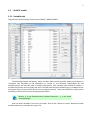
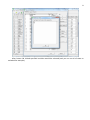
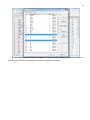
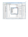
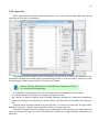
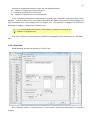
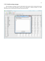
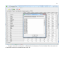
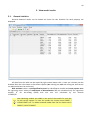
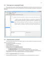
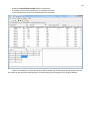
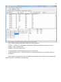
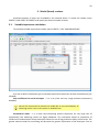
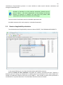
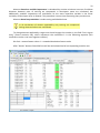
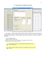
 CF program User manual (for working with RandomForest projects) 2
Changes: Date (program version) 03.02.09
(1.27)
Chapter First release version.
1
27.02.09
(1.28)
6
4
18.03.09
(1.29)
11.06.09
(2.00)
25.09.09
(2.03)
05.11.09
(2.04)
21.11.09
(2.05)
10.01.10
(2.06)
Description 1
Predicted values for oob-set compounds can now
be viewed on the “Forest statistics” tab.
Working with case set files was improved.
Specified model can be deleted from the model list
(menu FOREST / DELETE FOREST)
New chapter was inserted.
“Options” menu with various settings was added
to the program.
Loading of multiple models to the same forest list
are allowed now.
Y randomization procedure was implemented.
Possibility of analysis of multi-target models was
added.
Each Y (property) can have its own weight at model
construction process.
Menu “Statistics” has been removed.
Menu “Rebuild forest” has been disabled.
Visualization of model statistics and details has
been changed and can be displayed for each Y
(property) separately.
Data-files can now contain missing values marked
as NAN.
RF algorithm speed was significantly boosted
Some interface elements were optimized for
working with numerous data
Two domain applicability measures were
implemented:
1) based on variable importance values (in
descriptor space considering their relative
importance)
2) based on each tree prediction (in space of
models)
Multi-threads calculation was implemented, which
can speed up very intensive calculation steps
Improve statistics calculation.
Found memory leaks were eliminated
Structure of the manual was considerably revised,
new chapters were added and obsolete ones were
deleted.
3
Content
1.
Creation of the first RandomForest project. .....................................................................................4
1.1. Load data file..............................................................................................................................4
1.2. Build RF model ...........................................................................................................................7
1.2.1.
Variables tab ......................................................................................................................7
1.2.2.
Cases tab ..........................................................................................................................11
1.2.3.
Forest tab .........................................................................................................................12
1.2.4.
Possible warning messages..............................................................................................14
2. View model results ..........................................................................................................................16
2.1. General statistics......................................................................................................................16
2.2. View single trees composing RF model ...................................................................................17
2.3. Detailed statistics and results ..................................................................................................17
3. Model (forest) routines....................................................................................................................20
3.1. Variable importance calculation ..............................................................................................20
3.2. Domain of applicability calculation..........................................................................................21
4. “Preset mode” of model construction.............................................................................................23
5. Model (files) routines.......................................................................................................................24
5.1. Saving model............................................................................................................................24
5.2. Opening model(s).....................................................................................................................24
6. Prediction of compounds properties which are in an external data-file. .......................................25
7. General information. .......................................................................................................................26
8. Afterword.........................................................................................................................................27
Important remarks are marked in such style.
Advices are marked in such style.
4
1. Creation of the first RandomForest project. 1.1. Load data file To create RandomForest project choose menu FILE / NEW PROJECT / NEW RANDOM FOREST
PROJECT
Select a file with source data in the dialog:
- rfd-file, this is own file format of CF program,
- dat-file, this is file format of MDA1 program from HiT-QSAR Software package,
- txt-file, plain text format, descriptors are in columns, cases (compounds) are in rows (see
example below). First row and column contain descriptors names and molecules names
correspondingly. If some values are missing then they should be represented as NAN textual value or
leave empty. Such missed descriptor values automatically replaced with special NAN value. Descriptor
values should be numerical only (restriction of the current version) else an error message will be
displayed and file will not be opened. (Program does not check all possible errors in txt-file, so be
careful and be sure that there are no errors in your data file).
If txt-file has been chosen to create new project following dialog window would be displayed.
One should select appropriate settings to load txt-file. If variables (descriptors) names are absent in
the first line of the file (uncheck corresponding box) program will give names automatically (Var1,
Var2 etc). Analogous procedure will be executed if case names are absent.
5
6
After successful loading of source data it will be displayed on “Data” tab.
There is no possibility to edit data.
7
1.2. Build RF model 1.2.1. Variables tab To grow forest (build model) choose menu FOREST / GROW FOREST.
The following window will appear. Select variables which will be used for model construction on
“Variables” tab. Variables can be dependent (Y, several Y’s are allowed), independent (X) and
excluded (which will not take part in model construction). Also variables type should be chosen. Y
variable can possess all three types (but each Y should have identical variable type), X variables can be
continuous type only (restriction of the current program version). To do these operation simply select
variable(s) in the list and click on the appropriate button.
Buttons Y, X and Excluded have keyboard shortcuts - y, x and space
correspondingly.
One can select variables in the list by its names. Click on the “Select by names” button and input
variables names (one variable name per line).
8
After button OK clicked specified variables would be selected (and you can set all of them as
excluded for example).
9
If you choose several Y’s then “Y weights…” button will be enabled and weights for each Y
(property) will be able to be assigned. All positive numbers are allowed.
10
11
1.2.2. Cases tab Select appropriate set of each case (compound) on the “Cases” tab. Possible values are training
(working) set, test set or excluded set.
The program allows to define up to 10 separate test sets. To set a case to the wanted test set
(second for example) one should specify corresponding number in “test set number” field (in our case
it is 2) and then select the case and click “External test” button.
Buttons Training, External test и Excluded have keyboard shortcuts –
w, t and space correspondingly.
It is possible to load and save case sets. Case sets saves simultaneously in two formats:
- rfs, internal format of CF program (it supports multiple test sets);
- wsf, format of MDA1 program from HiT-QSAR Software package for backward compatibility
purpose (it supports only one test set, all test sets (if more than one) are saved as one entire test
set).
Program keeps 10 latest loaded and saved set-files. To view list of them click by right mouse
button on “Load set…” button. Latest used files will be on the top of the list.
Full path to selected set file in popup menu are displayed in the status bar just under the list of
cases. If opened set file was not find in its location the respective message would be appeared in the
status bar.
12
-
Statistics of compound numbers in each set are displayed below:
ws – number of compounds in the training set;
ts – number of compounds in all test sets;
exc – number of compounds in the excluded set.
If one Y variable selected and it has ranked or nominal type (“Variables” tab) then button “Class
weights…” will be enabled. Click it and following window will appear where one can define weights of
each compound class. Case weights can be integers only. This window is analogous to previously
described “Y weights…” dialog from “Variable” tab.
It is recommended to leave all values equal to 1 because testing of this
option is in progress now.
Function of “Select by names” button is absolutely analogous to the same button on “Variables”
tab.
1.2.3. Forest tab Model building settings are defined on “Forest” tab.
Here “Ordinary mode” » is described only. “Preset mode” will be described below in a separate
chapter.
13
It should be input in the table:
- Trees – the number of trees in the Random Forest model;
- Vars – the number of variables (descriptors) which will be used for splitting in each node of
trees. If one input this value which will be greater then available descriptors number this value will be
reduced automatically at the calculation step.
- Min parent and Min child – it is a minimum number of cases (compounds) in the parent or
child nodes. It can not be greater then 1/3 from the number of training set compounds. Otherwise
warning message will appear and this model will not be constructed.
In the original algorithm there are no such restriction parameters. All
trees are growing for their maximum size. So we recommend to use 1
as a value of “Min child” and “Min parent” fields for classification tasks.
For regression task to greater numbers can be assigned for these
values to increase calculation speed (for example Min parent = 5),
usually it has no influence on model quality
- Models – it is the number of models which will be constructed according to specified settings.
When all fields in one row are filled with non-zero values another row is appeared. This new row
one can fill with new settings. Thus a queue (package) of tasks is formed. Press Ctrl+Del to delete
selected row in the table.
In the case of very big datasets (thousands of cases and variables)
models construction consumes considerable memory size. So be
careful when you choose forest growth settings. And be sure that you
have enough memory to complete all your needed operations.
A method of training set formation of each tree is specified in the OOB set mode options dialog:
- Bootstrap – it as a classical mode of formation of training and out-of-bag sets for each tree
construction (with replacement).
- Custom – user can specify parts of cases of training and out-of-bag sets (without replacement).
Experience is shown that models which constructed in the second
(custom) mode have not appreciable changes in their quality. In
addition there is only little difference in model construction time. So
we recommend to choose the first (classical) mode (bootstrap).
Each model can be constructed with randomized Y values (Y randomization). To define part of Y
values which will be shuffled at model building one should check “Mix” field and choose
corresponding value from the range 0-100. If 100% value was chosen it would be Y scrambling
procedure. This procedure is used to prove that obtained model isn’t random.
14
1.2.4. Possible warning messages After OK button is pressed, if there are descriptors with constant and/or missing values among
X’s then a list with those descriptors names will be appeared in separate windows. All these
descriptors will be removed from the model construction process.
15
Progress of model construction is displayed in the bottom of main window. After that statistics
of obtained model is calculated for each case set.
16
2. View model results 2.1. General statistics General obtained results can be looked on Forest list tab. Statistics for each property are
displayed.
All data from this table can be copied by right mouse button click. A case set is shown into the
brackets after the value name in the column caption (ws–training set, oob–out-of-bag set, ts–first test
set, ts2–second test set and so on).
Risk estimate value is a misclassification error for classification models and mean square error
for regression ones. Values of coefficients of determination (R2) are calculated only for regression
models. R2 for out-of-bag (OOB) and test sets are calculated by the formula
1-PRESS/SS.
New obtaining models are added to the end of the models list until the
list will not be cleared. To clear the models list choose menu FOREST /
CLEAR FOREST LIST. To delete selected model from the list choose menu
FOREST / DELETE FOREST
17
2.2. View single trees composing RF model To do that select model in the list by left-click and switch to Trees tab. Each tree in the list can
be selected and viewed. Due to of a little importance of such information only general information is
displayed.
2.3. Detailed statistics and results To do that make double click on the model in the list or select model in the list by left-click and
switch to Forest Statistics tab.
The following information are displayed:
1) compound name
2) set to which compound belongs
3) observed values of investigated properties
4) predicted values of investigated properties
- for regression models it is a mean of all single tree predictions;
- for classification models it is a class having majority of votes (one tree–one vote).
5) is compound inside (sing “+”) or outside (sing “-“) of domain of applicability (several domain
of applicability measures were implemented and will discussed separately)
Additional regression model specific information:
1) standard deviation (StdDev) – it is calculated from set of predicted values by each tree
18
Additional classification model specific information:
1) number of each class predictions (in separate columns)
2) misclassification matrix (on the bottom of the window)
There is a possibility to filter results by property and/or set. Selecting certain property from the
list allows to see detailed model property corresponding specified property (see figure below).
19
For regression models following measures are calculated:
1) R2 – determination coefficient (reliable for training set only)
2) R2test – coefficient is calculated as 1-PRESS/SS (reliable for OOB, test and external sets)
3) MSE – mean standard error
4) RMSE –root mean square error
For classification models following measures are calculated:
1) Misclassification error – ratio of number of erroneous predictions to the whole number of
predictions
When domain of applicability was calculated corresponding values based on set of compounds
inside of domain of applicability are displayed.
20
3. Model (forest) routines. Unlimited number of trees can be added to the selected forest. To make this choose menu
FOREST / ADD TREES TO FOREST and specify the desired number of trees.
3.1. Variable importance calculation To calculate variable importances choose menu FOREST / CALC VAR IMPORTANCE.
User has to define calculation type of variable importances (selection of both simultaneously are
allowed).
Sum coefficients for each descriptor – it is a very fast and very rough estimate (temporarily
disabled).
We do not recommend to choose this mode due to very low adequacy of
obtaining results. Due to this option is disabled now.
Permutation mode – it is a more time-consuming process (especially for very large sets of
compounds). But obtaining results are highly adequate. This calculation based on estimation of
influence of randomization of each descriptor values on out-of-bag prediction ability of the forest. The
greater statistic values for out-of-bag set decrease the greater importance of the descriptor. Due to
21
randomness of permutation process it is more reliable to make several iterative calculation and
average of obtained result.
Numbers of iterations is a fully arbitrary parameter. However we can
give an advice – the more compounds in the training set the less
number of iterations is needed. For huge data sets (about 1000
compounds and more) one iteration can be enough.
To view results of calculation switch to Variable importance tab.
Variables importance for each property is calculated separately.
3.2. Domain of applicability calculation To calculate domain of applicability measures choose FOREST / CALC DOMAIN APPLICABILITY
In the opened dialog you can select desired domain applicability measure.
Measure based on trees prediction calculated by creation minimum-cost-tree. Distance s
between pairs of training set compounds in models space are considered. That is each model has T
number of predictions made by each tree in the model (T - total number of trees). Each prediction is
considered as a separate dimension. Thus Euclidean distance can be calculated.
22
Measure based on variable importance is calculated by creation minimum-cost-tree. Euclidean
distances between pairs of training set compounds in descriptors space are calculated, but
additionally variables importance are considered. So the more important variable is the lesser
variability of descriptor value is allowed. This procedure is more time-consuming than previous one.
Measure based on proximities is under testing and disabled now.
In all calculations of domain applicability only training set compounds
having observed values are considered.
To change domain applicability ranges one should change the number in the field “DA in sigma
units” (Forest statistics tab), which represents the coefficient k in the following equation (this
coefficient can be a real non-negative number).
DA limit = mean distance value + k × standard deviation distance value After “Recalc” button clicked DA limit will be recalculated and all corresponding statistics too.
23
4. “Preset mode” of model construction. This option is needed to collect statistics of huge number of models on the base of predefined
settings (possibility of saving of individual models is absent in this mode). This procedure is useful to
investigate forest behavior in a wide range of setup variables (number of trees and number of
descriptors).
-
There should be defined:
number of models of each type;
possible number of trees and descriptors for splitting (one value per line);
log-file name, where all results are saved.
In this mode “Min parent” and “Min child” parameters equal 1 and
cannot be changed.
Data is saved in the log-file as soon as it is produced. So there is no risk to
lost data.
24
5. Model (files) routines. 5.1. Saving model One can save model in a file by choosing FILE / SAVE PROJECT. Model saves into several separate
files:
1) .rf file – has a plain text format and contains general information, which can be useful for user
2) .t file – has a binary file format and contains all trees composing the model
3) .bin - has a binary file format and contains all data concerning the model and all statistics for
training, OOB and test sets (information and statistics of external set doesn’t save in the file)
4) .imp - has a binary file format and contains information concerning variable importances (if
they are calculated of course)
All these files are needed for model opening and should be stored in the same directory.
If the source file of the data set is not an rfd-file then at saving one should specify rfd-file name
(which will be contain a data set) and then rf-file name (which will be contain model information).
Rfd-file has an associated rfn-file of the same name. Both of them are
store source data and needed to successful data loading.
If rfd-file was created once try to use only it to create new projects for
the same data set. This can keep free space on HDD. Otherwise each
time new rfd-dile will be created.
5.2. Opening model(s) To open model use standard menu FILE / OPEN PROJECT
To open model it is necessary that data file (rfd-file) is in its initial directory (where it has been
saved first time) or in the same directory with rf-file.
1) one can freely move models on the computer, if place of corresponding rfd-file will be initial
2) one can copy model to USB stick and transfer it to another computer, but it is necessary to
copy all model files and associated rfd/rfn-files into the same directory
One could add saved models to the current forest list if they have identical associated data-file
(rfd-file).
1) if one try to open model file and data-file name will be identical to already opened model
then the new model will be added to the list.
2) if one model has been already opened than one can select menu FILE / ADD MODELS TO THE
CURRENT LIST to proceed. In opened dialog only models having according associated data-file
will be displayed. Selection of multiple files is allowed.
25
6. Prediction of compounds properties which are in an external data‐file. To make prediction of compounds in an external data-file select the desired model in the model
list and choose menu PREDICTION / PREDICT DATA FROM FILE.
If the open file has a variable with the same name as a target property then this file will be
recognized as an external test set and the corresponding statistics will be calculated.
After prediction process was complete new set named “ext1” will be added to the list of model
sets on Forest statistics tab. There one can select this set from the list, or select certain property to
look for detailed statistics. As results of external data prediction don’t save to model file one can find
it useful to copy and paste this information in external editor.
26
7. General information. To copy data from various lists and tables one can often use right-mouse clicking and chosing
appropriate item in popup menu.
Current program version is displayed in window which is call via menu ABOUT.
27
8. Afterword. Do not hesitate to contact us if you found mistakes, faults, unusual program behavior or
program failure or had any questions or ideas to improve program algorithm or interface! Any advices
are welcome and will be taking in consideration at next version development!
28
ABOUT............................................................ 25
ADD MODELS TO THE CURRENT LIST............. 23
ADD TREES TO FOREST................................... 19
CALC DOMAIN APPLICABILITY........................ 20
CALC VAR IMPORTANCE ................................ 19
CLEAR FOREST LIST......................................... 15
DELETE FOREST .............................................. 15
GROW FOREST ................................................. 7
NEW FANDOM FOREST PROJECT......................4
NEW PROJECT ...................................................4
OPEN PROJECT ................................................23
Ordinary mode................................................11
PREDICT DATA FROM FILE ..............................24
Preset mode....................................................22
SAVE PROJECT.................................................23