Download MANUEL D`UTILISATION ISIDA

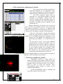
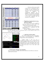
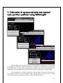
USER MANUAL
FOURCHES Denis
2006
1
Summary
-
1. Data Preparation
o Data randomization
o Duplicates search
o Scrambling
-
2. Calculation of descriptors
o Calculation of molecular fragments
o Variables selection
o How to split an entire dataset into a training/test sets
o Export data and convert them into different files formats.
-
3. Data and descriptors analysis
o According to property classes
o According to descriptors classes
o Statistical criteria of descriptors
o Correlation matrix of descriptors
o Replacement of a descriptor by another correlated one.
-
4. Principal Components Analysis (PCA)
o Settings – Parameters of calculations
o 3D view and tools
o Color compounds according a property or a cluster analysis
-
5. Cluster Analysis (“clustering”) using ISIDA/Cluster
o Setting – Parameters of calculations
o Dendogram representation and tools
o Clusters explorer
o Proximity maps (IPM/FPM)
o Export clusters and data
o Property explorer
-
6. QSPR modelling using ISIDA/kNN
o Initial parameters – Mode “Advanced user”
o Selection of predictive models
o Property predictions of external set compounds using selected models
o Load/Save kNN models
-
7. Calculation of aqueous solubility and octanol/water partition coefficient using
ISIDA/LogPS
-
8. ISIDA/DC models : (in progress)
o Modelling architect
2
1. Data Preparation
o Data randomization
Most of the SD files containing molecules libraries are sorted, i.e. the compounds inside a SD
file are ranked according to a parameter. ISIDA includes a randomization option to avoid any
problem.
To randomize your data, please click on “Descriptors” in the ISIDA wizard. Select your SD
file with the “Open SD FILE” button, and click on “Randomize”. A new SD file is created,
having the same name than the previous one, but the extension “_R.sdf” is added.
o Duplicates search
Detecting duplicates in a large database is not a common task and cannot be done without a
computational help.
To search duplicates, be sure that you have the SD file and a corresponding SMF file
(containing descriptors) in the same directory. Select the SMF file with the “Open” button and
the name of the property. Click on “Analyse” to launch the procedure.
To go from one duplicate to another, use the control panel. Be careful: the program finds also
isomers.
o Scrambling (not finished and not available outside ISIDA/DC models)
3
2. Calculations of descriptors
o Calculation of molecular fragments
Click on the “Descriptors” button in the top of the
wizard. Select your SD file in the “Descriptors”
window.
All molecular fragments are available in the
“Fragmentation settings”. User can select and/or
unselect a given type of fragments, and modify
the range of their length (from 2 to 6 by default).
The “All Fragments” checkbox allows user to
select in only one click ALL types of molecular
fragments.
The “External descriptors” checkbox activates the
so-called name groupbox, in order to select a file
containing columns of external descriptors for
this dataset. [At this time, this option is only
available in the ISIDA/cluster v1 and not in ISIDA/cluster v2]
The “Calculate Fragments” button launches the fragmentation of compounds, and creates a
SMF (Substructural Molecular Fragments) file. At the end of calculations, the number of
compounds and descriptors are written in the memo, and then, two buttons are visible:
“Variables selection” and “Files convertor”.
o Variables selection
The variables selection suite of ISIDA includes several approaches and options, which can be
used successively.
4
-
Checkbox 1: suppress fragments which have an positive occurrence in less than m
molecules, m being a user-defined threshold;
Checkbox 2: keep only fragments which are present in the CFR file (selected by user),
corresponding to the list of fragments involved in a linear QSPR model performed by
ISIDA/QSPR;
Checkbox 3: keep only fragments selected by the Unsupervised Forward Selection
(UFS);
Checkbox 4: suppress high correlated fragments (R2 > user defined threshold);
Checkbox 5: suppress low correlated fragments with the studied property (R2 < user
defined threshold) [Click on “Files convertor” to select the property]
Checkbox 6: calculate the p principal components of the variables and keep only the p
variables in the SMF file. [Available in ISIDA v1; not finished in ISIDA v2].
Click on the “Create Files” button to launch the selection of variables. The new SMF is
created automatically and has a new extension “_SEL.SMF”.
Recommendation: use the “Files convertor” together with the “Variables selection”.
o Splitting data into training/test sets
Click on the “Files convertor” button to access to all available options, and click on the
“Mask Editor” button.
In the left part of the window, a grid of white squares represents the compounds of the entire
set. The Mask Editor allows user to split the data into subsets.
The “MANUAL SELECTION ON/OFF” button (des-) activates the manual selection of compounds
with the mouse. A left click on any compound colors the corresponding square in gray, and
puts the selected compound into the test set.
5
WHITE = training set
-
GRAY = test set
Radiobutton 1: put each ith compound in the test set starting from the number j.
Radiobutton 2: put the first i compounds in the test set.
Radiobutton 3: put the last i compounds in the test set.
Random selection: user can also indicate the number of compounds in the test set, or the
percentage of compounds on the entire set. From this number, the program selects randomly
the desired number of compounds.
[The random selection for the external set is not finished]
When the splitting is terminated, two saving modes are available:
- Using a msk file: if user wants to create input files for ASNN, WEKA, or ISIDA/QSPR,
he has to save his work in a *.msk file using the “SAVE MSK FILE” button.
- Using SD files: if user wants to use ISIDA/kNN or ISIDA/Cluster, he has to save his
work in two SD files (one including compounds of the training set, another one for the
test set) using the two buttons: “Training Set : export SDF” and “Test Set : export SDF”.
[The “External Set : export SDF” button is not finished].
Clusters: not finished.
o Export data – Convert into different formats
Click on “Files convertor” and select the property, the mask file and the formats of output
files (SMF is always created). Press “Create Files”.
The new files have been written in the same directory than the initial SD and SMF files.
6
3. Data and descriptors analysis
o According to property classes
The Data Analysis module of ISIDA allows one to split its data according to a numerical
property: property classes. This feature is useful to visualize the distribution of a dataset of
compounds according to the studied property or activity.
To perform the analysis, select the dataset and the property. Specify the number of classes (10
by default) and click on “Analyse”.
The X axis corresponds to the property and the Y axis corresponds to the number of
compounds. Each histogram represents an ensemble of compounds having similar property
values. The scale of the X axis is derived automatically from the desired number of classes.
If the user wants classes with a given range of property, he has to enter this value in the edit
under the “Fixed scaling” checkbox (has to be checked) and then “Analyse” again.
If the user wants to change the minimal and the maximal value of the X axis, he has to enter
the corresponding values in the two edits under the “Fixed Min/Max Property” checkbox (has
to be checked) and then “Analyse” again.
7
o According to descriptors classes
One click on the “Analysis of descriptors” button opens another part of the data analysis
module of ISIDA, performing a splitting of data according to descriptor classes (the SMF file
and the SD file having the same name have to be in the same directory. Else, a SMF file has
to be created).
“DISTRIBUTION MODE’: the program reads the SMF file and fills the left tree view with
the list of calculated descriptors for the set. If the user clicks on a particular fragment,
compounds are sorted according to the occurrence of the fragment: several histograms are
drawn corresponding to the different occurrences (X axis) that take the studied fragment, in
order to show the number of compounds (Y axis) having each occurrence.
A given histogram can be selected using the “Select Mode” button. Then, the compounds
having this occurrence of the studied fragment are displayed in the right listbox with their
experimental property. User can also look at structures by clicking one compound in the list.
The “Hide zero fragment” hides the compounds having not the studied fragment. This option
leads to a new scale of the Y axis.
“QSAR
VIEW
MODE”:
the
experimental property is projected on
the X axis and the number of
occurrences of the selected fragment
on the Y axis. Each red point is a
compound, whose the structure can be
seen with a mouse move on it.
8
This QSAR view represents a graphical mode to detect correlations between an experimental
property and variables.
The program includes also the ability to treat external descriptors. If they are not fragments,
and take real values, the occurrences are replaced by ranges in the “DISTRIBUTION
MODE”, and by real values in the “QSAR VIEW MODE”. [Available in ISIDA v1; not
finished in ISIDA v2]
o Statistical criteria of descriptors
Click on “Calculate Statistics” and “Save File”. A text file is created in the work directory
including:
-
the name of the set;
the number of compounds;
the number of fragments;
the name of the studied property;
for each descriptor:
 the symbol of the fragment (ex : C – C – C);
 the number of descriptors classes (= number of different occurrences taken
by the descriptor)
 the correlation coefficient R (and R2) between the descriptor and the
property
 the frequency of the fragment in the set
 the number of compounds having this fragment
 the total number of occurrences of this fragment
 a warning if less than only 5 compounds in the set have this fragment.
9
The “Sort descriptors” procedure is not finished. Click
CORRELATION” to see the correlation matrix between descriptors.
on
“DESCRIPTORS
o Correlation matrix of descriptors
ISIDA builds the correlation matrix between descriptors after one click on “Analyse”. User
can easily detect pairs of high correlated variables.
o Replacement of a given descriptor by another correlated one.
10
If user wants to search correlated variables for a given descriptor, ISIDA allows one to filter
the variables and visualize the correlation (X axis: studied descriptor; Y axis: correlated
descriptor). Results can be saved in the “Correlated_Descs_List.txt”.
11
4. Principal Components Analysis (PCA)
o Settings – Parameters of calculations
SD and SMF files have to be in the same directory and use the “Open SDF/SMF” button to
select one of them. If no information appears in the “Available Data” combobox, it means that
no previous PCA calculations are available for this set in the work directory.
The “Calculate” button can be clicked if user has entered a number of components (3 by
default).
If previous calculations are available, select the corresponding line in the combobox and click
on the “DISPLAY” button.
o 3D view and tools
12
To rotate the points, the left button of the mouse has to be down, and the rotation is made
according to the mouse move.
To zoom in or out of the points, the right button of the mouse has to be down, and the zoom
coefficient is calculated according to the mouse move.
User can assign one of the calculated components to one (or more) axis. By default, the X axis
corresponds to the first principal component; the Y axis corresponds to the second principal
component, and the Z axis to the third principal component. For each component, the program
calculates the percentage of the total variance of variables expressed by the given component.
A graphical representation can be displayed by clicking on the “VAR” button, and the
percentages are written in green near the selected components.
o Coloring points according to a property value or to clusters
13
Color by property: there is a dedicated combobox (under the “Select property” label) to
select the property. Then, select “Color by property” in the Color settings combobox. User
can adjust the number of property classes with the appropriate trackbar.
Color by clusters: ISIDA/Cluster creates FCL files (File of Classes) to save the results
(contents of clusters) for each clustering. Click on “Open FCL file” to select the FCL
corresponding to the studied set, and then, select “Color by cluster” in the Color settings
combobox.
Remark: the “Use reduced SMF” checkbox can be used to calculate PCA with the selected
variables of a “******_SEL.SMF” (see variables selection).
14
5. Cluster Analysis (“clustering”) using ISIDA/Cluster
o Settings – Parameters of calculations
 if the SMF file is available:
Click on the “Clustering” button in the ISIDA wizard, and select the SMF with the “Open
SMF file”. The number of compounds, the type of fragments and the number of fragments are
displayed under the name of the SMF file.
 if the SMF file is not available:
Click on the “Descriptors” button in the ISIDA wizard to calculate fragments for the studied
dataset. Once the SMF file has been created (see 2.Calculation of descriptors), click on the
“Clustering” button in the ISIDA wizard, and select the SMF with the “Open SMF file”. The
number of compounds, the type of fragments and the number of fragments are displayed
under the name of the SMF file.
Several parameters are required for cluster analysis.
By default, the clustering is entirely hierarchical,
with a Euclidian metric between compounds, and a
complete link between clusters, descriptors are not
normalized and no modified metric is employed.
User can modify these parameters using the menu on
the top of the ISIDA window.
In the “metric between compounds” menu, the
“Tanimoto similarity” corresponds to the distance
calculated as:
Dist(i,j) = 1 – TANIMOTO(i,j)
The calculations begin if the „launch” button is pressed.
15
o Dendogram representation and tools
When the calculations stop, click on the “View Dendogram” button. A new window is
maximized and the resulting dendogram is drawn.
The exploration of any part of the dendogram is easy with the small dynamic circles placed on
the dendogram itself. A left click on any circle (the circle is activated -> blue color) results in
the display of the list of compounds (in the left listview of the window) deriving from this
circle.
If the circle is activated (blue), a right click on this circle
leads to the display of a popup window, including the
option to define cluster.
When a cluster is defined, all the selected compounds are
assigned to this cluster. User can also define sub-clusters
which are clusters included in bigger clusters (nonexclusive clustering): that means that a particular compound
can eventually belong to several clusters.
The list of selected clusters is shown in the left listview, near the color pattern. To explore in
details the contents of the clusters, click on “Show clusters” after the selection of clusters.
16
o Clusters explorer
The clusters explorer is dedicated to see in details the contents of the selected clusters, with
histograms of the clusters sizes, two control panels to explore the clusters and the molecules
inside one given cluster, Tanimoto similarity calculator for clusters …
o Export clusters
The clustering program saves the results in FCL file containing the IDs of compounds for
each cluster, and a COF file containing the different parameters used to perform the cluster
analysis.
User can also save in SD files the contents of clusters using the “Export SDF” page in the
Clusters explorer.
17
To save one cluster, write the ID of the cluster (example: write 1 for cluster 1) and the name
of the SD file. Click “Ok”.
o Proximity maps (IPM/FPM)
IPM
FPM
Click on the “First Proximity Matrix Explorer” button to launch the viewer of proximity
maps. This viewer is dedicated to the visualization of the proximity matrix of compounds
before the clustering (IPM: Initial Proximity Matrix) when compounds are not sorted, and
after the clustering (FPM: Final Proximity Matrix) when compounds are sorted according to
the final arrangement from the cluster analysis.
18
Each point of the map represents the distance between the compounds i and j. The IPM is first
displayed. Click on the “Clustering effects” button to visualize the FPM, and click on the
“Tanimoto Visualisation” to color the FPM with a Tanimoto similarity color pattern.
DISTANCE MODE: red -> blue corresponds to “small distances” -> “big distances”
TANIMOTO MODE: red -> blue corresponds to “non similar” -> “very similar”
Histograms on the right represent the distribution of distances for all pairs of compounds. In
the example below, there are a low number of minimal and maximal distances, but a huge
number of intermediate distances.
o Property explorer
User can search for a cluster having an
homogeneous activity. The property
explorer allows one to show the
property classes inside each cluster.
Select the property and a number of
classes, and click on “Show Property”.
This module is not finished.
19
6. Perform QSPR modelling using ISIDA/kNN
Fig. X: Control panel of the ISIDA/kNN program.
o Initial parameters
Three sets are required for the modelling: (i) the training set, (ii) the internal test set
and (iii) the external set. Three Open Dialog boxes can be opened by clicking on the Open
buttons, in order to select the corresponding datasets in the appropriate directory. Then, the
program analyses the SD file to search for all available fields. Thus, the user can choose the
property (in the ComboBox) for the modelling.
To launch the kNN calculations with parameters by default, the “Run new
calculation” button has to be clicked.
o Mode “Advanced user”
This mode allows user to modify the settings used for the kNN calculations. The full
window appears after that the checkbox “Advanced user” has been clicked.
The “Descriptors” page is dedicated to the type
of molecular fragments taken into account for the
calculations, and also the minimal and the maximal
number of variables that models can contain.
The “kNN settings” page allows user to select
the type of normalization (none by default) to apply to
descriptors, the range of nearest neighbors to examine
(from 2 to 5 by default), the randomization key (0 by
default), the metric between compounds (euclidian by
default).
The “Variable selection” page is split in two
parts: the left part concerns the deletion of variables
before kNN calculations: correlated fragments, constant
fragments or with low variance etc. The right part
concerns the variables selection for the kNN
calculations: user can modify the maximal number of
iterations between two steps of the forward stepwise
variable selection (1000 by default).
The “Property” and “Compounds” pages are
only accessible at the end of calculations.
To launch kNN calculations, the “Run new calculation” button has to be clicked.
20
o kNN calculations: displaying of results
The program starts with the calculation of
molecular fragments for all compounds. Then,
some of these descriptors are deleted due to their
high correlated coefficient or their low variance.
The kNN procedure begins with the
generation of a user-defined number of models
involving m descriptors. Among them, the
stepwise variable selection algorithm selects the
best ones according to Q2 (LOO procedure), or
optionally, according to the R2 obtained for the
internal test set.
During calculations, at any time, the user has an
entire access to the available models: a list of the tenth
best models (according to their Q2) is displayed and
updated each time that a new model having a best Q 2 ever
is discovered. The number of models is also displayed.
This list of “hit models” contains the statistical
criteria for each model: the number of involved
variables; the number of neighbors; Q2 and RMSE for the LOO procedure (on the
training set); R2, RMSE, the coefficients of the
linear regression: PRED = a + b* EXP for the test
set.
On the “BATCH CURVES” page, some graphical
representations of results are available: curves of
statistical criteria versus the number of iterations;
R2 (for the test set) versus Q2 (for the training set)
for all available models; the calculated (LOO)
property values versus the experimental ones for
the training set; the predicted property values
versus the experimental ones for the test set.
Calculations stop when the maximal number of variables has been reached, or
when the “STOP” button has been clicked.
o Selection of predictive models
ISIDA/kNN produces a huge number of
models with high or low predictive abilities. In order
to select the most predictive ones, the user can choose
adequate values of Q2 and R2 in the “FILTER MODELS”
panel in order to make the selection. These
corresponding models appear in yellow on the
graphical representation.
On the “ListMODELS” page, a worksheet has
been filled with the selected models.
21
If the user clicks on any model
in the list, the “Compounds” page is
available: for each compound of the
test or the external set, it is possible to
visualize
its
neighbors,
the
experimental
properties
of
its
neighbors, the similarity coefficients.
Thus, user can assess if it is reasonable
or not to predict the studied property
of the given compound with the
properties of its neighbors.
o Prediction of external set using
selected models
The selected models can be applied to
screen the external set, with a click on the
“Apply models to external set” button.
A new worksheet is filled with each line
corresponding to a compound and each
column for a model.
Press the “Mean/SD” button to calculate,
for each compound, the mean (“consensus model”) of the predicted values by all
models and the standard deviation.
o Load/Save kNN models
User can save model one by one, or all together.
Each model is saved individually in a *.MOD file.
Saving models is done instantaneously.
Loading models is also very easy to
accomplish: the program must be restarted and the
“LOAD MODELS” button pressed. Then you can
reload models one by one or all together. (Be careful:
the SD files of the training, test and external sets, and
the MOD files have to be in the same work
directory).
o PCA/Cluster Analysis (in progress)
These two options are available when some models have been filtered, or when one
model has been selected.
22
7. Calculation of aqueous solubility and octanol/
water partition coefficient using ISIDA/LogPS
ISIDA/LogPS reads mol and SD files. User can launch calculations of logP and logS
by clicking the “Calculate” button. During the calculations, the distribution of compounds
according to their corresponding calculated logS or logP is represented with histograms and
updated at every compound. User can choose to visualize the histograms of logP or logS.
Once calculations are ended, one click on “Show Results” leads to the displaying of
the predicted values for each compound. The “Update SD file” allows user to insert
automatically these predicted values as new fields in the studied SD file:
23
-
a numeric field containing the predicted logS value;
a numeric field containing the predicted logP value;
a textual field containing “Soluble” or “Insoluble”.
24
8. ISIDA/DC models (in progress)
25