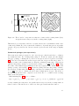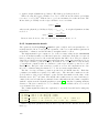
1
Physics Physics Department, Technical University of Denmark 2800 Kongens Lyngby, Denmark Component Manual for the Neutron Ray-Tracing Package McStas, version 2.1 P. Willendrup, E. Farhi, E. Knudsen, U. Filges, K. Lefmann September, 2014 The software package McStas is a tool for carrying out Monte Carlo ray-tracing simulations of neutron scattering instruments with high complexity and precision. The simulations can compute all aspects of the performance of instruments and can thus be used to optimize the use of existing equipment, design new instrumentation, and carry out virtual experiments for e.g. training, experimental planning or data analysis. McStas is based on a unique design where an automatic compilation process translates high-level textual instrument descriptions into efficient ISO-C code. This design makes it simple to set up typical simulations and also gives essentially unlimited freedom to handle more unusual cases. This report constitutes the reference manual for McStas, and, together with the manual for the McStas components, it contains documentation of most aspects of the program. It covers the various ways to compile and run simulations, a description of the meta-language used to define simulations, and some example simulations performed with the program. This report documents McStas version 2.1, released September, 2014 The authors are: Peter Kjær Willendrup <[email protected]> Physics Department, Technical University of Denmark, Kongens Lyngby, Denmark Emmanuel Farhi <[email protected]> Institut Laue-Langevin, Grenoble, France Erik Knudsen <[email protected]> Physics Department, Technical University of Denmark, Kongens Lyngby, Denmark Kim Lefmann <[email protected]> Niels Bohr Institute, University of Copenhagen, Denmark as well as authors who left the project: Peter Christiansen <[email protected]> Materials Research Department, Risø National Laboratory, Roskilde, Denmark Present address: University of Lund, Lund, Sweden Klaus Lieutenant <[email protected]> Institut Laue-Langevin, Grenoble, France Present address: Helmotlz Zentrum Berlin, Germany Kristian Nielsen <[email protected]> Materials Research Department, Risø National Laboratory, Roskilde, Denmark Presently associated with: MySQL AB, Sweden ISBN 978–87–550–3680–2 ISSN 0106–2840 Information Service Department · Risø DTU · 2015 Contents . Preface and acknowledgements 1. About the component library 1.1. Authorship . . . . . . . . . . . . . 1.2. Symbols for neutron scattering and 1.3. Component coordinate system . . . 1.4. About data files . . . . . . . . . . . 1.5. Component source code . . . . . . 1.6. Documentation . . . . . . . . . . . 1.7. Component validation . . . . . . . 1.8. Disclaimer, bugs . . . . . . . . . . 10 . . . . . . . simulation . . . . . . . . . . . . . . . . . . . . . . . . . . . . . . . . . . . . . . . . . . . . . . . . . . . . . . . . . . . . . . . . . . . . . . . . . . . . . . . . . . . . . . . . . . . . . . . . . . 2. Monte Carlo Techniques and simulation strategy 2.1. Neutron spectrometer simulations . . . . . . . . . . . . . . . 2.1.1. Monte Carlo ray tracing simulations . . . . . . . . . 2.2. The neutron weight . . . . . . . . . . . . . . . . . . . . . . . 2.2.1. Statistical errors of non-integer counts . . . . . . . . 2.3. Weight factor transformations during a Monte Carlo choice 2.3.1. Direction focusing . . . . . . . . . . . . . . . . . . . 2.4. Adaptive and Stratified sampling . . . . . . . . . . . . . . . 2.5. Accuracy of Monte Carlo simulations . . . . . . . . . . . . . . . . . . . . . . . . . . . . . . . . . . . . . . . . . . . . . . . . . . . . . . . . . . . . . . . . . . . . . . . . . . . . . . . . . . . . . . . . . . . . . . . . . . . . . . . . . . . . . . . . . . . . . . . . . . . . . 3. Source components 3.0.1. Neutron flux . . . . . . . . . . . . . . . . . . . . . . . . . . . . . 3.1. Source simple: A simple continuous source with a flat energy/wavelength spectrum . . . . . . . . . . . . . . . . . . . . . . . . . . . . . . . . . . . 3.2. Source div: A continuous source with specified divergence . . . . . . . . 3.3. Source Maxwell 3: A continuous source with a Maxwellian spectrum . . 3.4. Source gen: A general continuous source . . . . . . . . . . . . . . . . . . 3.5. Moderator: A time-of-flight source (pulsed) . . . . . . . . . . . . . . . . 3.6. ISIS moderator: ISIS pulsed moderators . . . . . . . . . . . . . . . . . . 3.6.1. Introduction . . . . . . . . . . . . . . . . . . . . . . . . . . . . . 3.6.2. Using the McStas Module . . . . . . . . . . . . . . . . . . . . . . 3.6.3. Comparing TS1 and TS2 . . . . . . . . . . . . . . . . . . . . . . 3.6.4. Bugs . . . . . . . . . . . . . . . . . . . . . . . . . . . . . . . . . . 3.7. Source adapt: A neutron source with adaptive importance sampling . . 3.7.1. Optimization disclaimer . . . . . . . . . . . . . . . . . . . . . . . . . . . . . . . 12 12 12 13 13 13 14 16 17 . . . . . . . . 18 18 18 19 19 20 21 21 22 24 . 24 . . . . . . . . . . . . 26 26 27 28 30 31 31 32 33 33 35 36 5 3.7.2. The adaption algorithm . . . . . . . . . . . . . . . . . . . . . . . 3.7.3. The implementation . . . . . . . . . . . . . . . . . . . . . . . . . 3.8. Adapt check: The adaptive importance sampling monitor . . . . . . . . 3.9. Source Optimizer: A general Optimizer for McStas . . . . . . . . . . . . 3.9.1. The optimization algorithm . . . . . . . . . . . . . . . . . . . . . 3.9.2. Using the Source Optimizer . . . . . . . . . . . . . . . . . . . . . 3.10. Monitor Optimizer: Optimization locations for the Source Optimizer . . . . . . . . . . . . . . . . . . . . . . . . . . . . . . . 3.11. Other sources components: contributed pulsed sources, virtual sources (event files) . . . . . . . . . . . . . . . . . . . . . . . . . . . . . . . . . . 4. Beam optical components: Arms, slits, collimators, and filters 4.1. Arm: The generic component . . . . . . . . . . . . . . . . . 4.2. Slit: A beam defining diaphragm . . . . . . . . . . . . . . . 4.3. Beamstop: A neutron absorbing area . . . . . . . . . . . . . 4.4. Filter gen: A general filter using a transmission table . . . . 4.5. Collimator linear: The simple Soller blade collimator . . . . 4.5.1. Collimator transmission . . . . . . . . . . . . . . . . 4.5.2. Algorithm . . . . . . . . . . . . . . . . . . . . . . . . 4.6. Collimator radial: A radial Soller blade collimator . . . . . . . . . . . 36 38 38 40 40 41 . 42 . 43 . . . . . . . . 44 44 44 45 45 47 47 47 48 5. Reflecting optical components: mirrors, and guides 5.1. Mirror: The single mirror . . . . . . . . . . . . . . . . . . . . . . . . . . 5.1.1. Mirror reflectivity . . . . . . . . . . . . . . . . . . . . . . . . . . 5.1.2. Algorithm . . . . . . . . . . . . . . . . . . . . . . . . . . . . . . . 5.2. Guide: The guide section . . . . . . . . . . . . . . . . . . . . . . . . . . 5.2.1. Guide geometry and reflection . . . . . . . . . . . . . . . . . . . 5.2.2. Algorithm . . . . . . . . . . . . . . . . . . . . . . . . . . . . . . . 5.3. Guide channeled: A guide section component with multiple channels . . 5.3.1. Algorithm . . . . . . . . . . . . . . . . . . . . . . . . . . . . . . . 5.3.2. Known problems . . . . . . . . . . . . . . . . . . . . . . . . . . . 5.4. Guide gravity: A guide with multiple channels and gravitation handling 5.5. Bender: a bender model (non polarizing) . . . . . . . . . . . . . . . . . . 5.6. Curved guides . . . . . . . . . . . . . . . . . . . . . . . . . . . . . . . . . . . . . . . . . . . . . 50 50 50 51 52 53 54 55 55 55 56 56 57 6. Moving optical components: Choppers and velocity selectors 6.1. DiskChopper: The disc chopper . . . . . . . . . . . . . . . . . . . . 6.2. FermiChopper: The Fermi-chopper . . . . . . . . . . . . . . . . . . 6.2.1. The chopper geometry and parameters . . . . . . . . . . . . 6.2.2. Propagation in the Fermi-chopper . . . . . . . . . . . . . . 6.3. Vitess ChopperFermi: The Fermi Chopper from Vitess . . . . . . . 6.4. V selector: A rotating velocity selector . . . . . . . . . . . . . . . . 6.4.1. Velocity selector transmission . . . . . . . . . . . . . . . . . 6.5. Selector: another approach to describe a rotating velocity selector . . . . . . . . 59 59 62 63 63 67 70 71 71 6 . . . . . . . . . . . . . . . . . . . . . . . . . . . . . . . . . . . . . . . . . . . . . . . . . . . . . . . . . . . . . . . . . . . . . . . . . . . . . . . . 7. Monochromators 7.1. Monochromator flat: An infinitely thin, flat mosaic crystal with a single scattering vector . . . . . . . . . . . . . . . . . . . . . . . . . . . . . . . 7.1.1. Monochromator physics and algorithm . . . . . . . . . . . . . . . 7.2. Monochromator curved: A curved mosaic crystal with a single scattering vector . . . . . . . . . . . . . . . . . . . . . . . . . . . . . . . . . . . . . 7.3. Single crystal: Thick single crystal monochromator plate with multiple scattering . . . . . . . . . . . . . . . . . . . . . . . . . . . . . . . . . . . 7.4. Phase space transformer - moving monochromator . . . . . . . . . . . . 8. Samples 8.0.1. Neutron scattering notation . . . . . . . . . . . . . . . . . . 8.0.2. Weight transformation in samples; focusing . . . . . . . . . 8.0.3. Future development of sample components . . . . . . . . . 8.1. Incoherent: An incoherent scatterer, the V-sample . . . . . . . . . 8.1.1. Physics and algorithm . . . . . . . . . . . . . . . . . . . . . 8.1.2. Remark on functionality . . . . . . . . . . . . . . . . . . . . 8.2. Tunneling sample: An incoherent inelastic scatterer . . . . . . . . . 8.3. PowderN: A general powder sample . . . . . . . . . . . . . . . . . . 8.3.1. Files formats: powder structures . . . . . . . . . . . . . . . 8.3.2. Geometry, physical properties, concentricity . . . . . . . . . 8.3.3. Powder scattering . . . . . . . . . . . . . . . . . . . . . . . 8.3.4. Algorithm . . . . . . . . . . . . . . . . . . . . . . . . . . . . 8.4. Single crystal: The single crystal component . . . . . . . . . . . . . 8.4.1. The physical model . . . . . . . . . . . . . . . . . . . . . . . 8.4.2. The algorithm . . . . . . . . . . . . . . . . . . . . . . . . . 8.4.3. Choosing the outgoing wave vector . . . . . . . . . . . . . . 8.4.4. Computing the total coherent cross-section . . . . . . . . . 8.4.5. Implementation details . . . . . . . . . . . . . . . . . . . . . 8.5. Sans spheres: A sample of hard spheres for small-angle scattering . 8.5.1. Small-angle scattering cross section . . . . . . . . . . . . . . 8.5.2. Algorithm . . . . . . . . . . . . . . . . . . . . . . . . . . . . 8.5.3. Calculating the weight factor . . . . . . . . . . . . . . . . . 8.6. Phonon simple: A simple phonon sample . . . . . . . . . . . . . . . 8.6.1. The phonon cross section . . . . . . . . . . . . . . . . . . . 8.6.2. The algorithm . . . . . . . . . . . . . . . . . . . . . . . . . 8.6.3. The weight transformation . . . . . . . . . . . . . . . . . . 8.7. Isotropic Sqw: A general S(q, ω) coherent and incoherent scatterer 8.7.1. Neutron interaction with matter - overview . . . . . . . . . 8.7.2. Theoretical side . . . . . . . . . . . . . . . . . . . . . . . . . 8.7.3. Theoretical side - scattering in the sample . . . . . . . . . . 8.7.4. The implementation . . . . . . . . . . . . . . . . . . . . . . 8.7.5. Validation . . . . . . . . . . . . . . . . . . . . . . . . . . . . . . . . . . . . . . . . . . . . . . . . . . . . . . . . . . . . . . . . . . . . . . . . . . . . . . . . . . . . . . . . . . . . . . . . . . . . . . . . . . . . . . . . . . . . . . . . . . . . 73 . 73 . 73 . 76 . 78 . 78 . . . . . . . . . . . . . . . . . . . . . . . . . . . . . . . . 80 80 81 83 83 84 85 86 88 89 90 90 92 94 96 98 99 101 102 104 104 105 105 106 107 107 108 109 111 111 113 119 123 7 9. Monitors and detectors 9.1. TOF monitor: The time-of-flight monitor . . . . . . . . . . . . . . . . 9.2. TOF2E monitor: A time-of-flight monitor with simple energy analysis 9.3. E monitor: The energy-sensitive monitor . . . . . . . . . . . . . . . . . 9.4. L monitor: The wavelength sensitive monitor . . . . . . . . . . . . . . 9.5. PSD monitor: The PSD monitor . . . . . . . . . . . . . . . . . . . . . 9.6. Divergence monitor: A divergence sensitive monitor . . . . . . . . . . 9.7. DivPos monitor: A divergence and position sensitive monitor . . . . . 9.8. Monitor nD: A general Monitor for 0D/1D/2D records . . . . . . . . . 9.8.1. The Monitor nD geometry . . . . . . . . . . . . . . . . . . . . . 9.8.2. The neutron parameters that can be monitored . . . . . . . . . 9.8.3. Important options . . . . . . . . . . . . . . . . . . . . . . . . . 9.8.4. The output files . . . . . . . . . . . . . . . . . . . . . . . . . . 9.8.5. Monitor equivalences . . . . . . . . . . . . . . . . . . . . . . . . 9.8.6. Usage examples . . . . . . . . . . . . . . . . . . . . . . . . . . . 9.8.7. Monitoring user variables . . . . . . . . . . . . . . . . . . . . . 9.8.8. Monitoring neutron parameter correlations, PreMonitor nD . . . . . . . . . . . . . . . . . . 125 . 126 . 126 . 127 . 128 . 128 . 129 . 129 . 131 . 132 . 133 . 133 . 134 . 134 . 134 . 136 . 138 10.Special-purpose components 140 10.1. Virtual output: Saving the first part of a split simulation . . . . . . . . . 141 10.2. Virtual input: Starting the second part of a split simulation . . . . . . . . 141 10.3. Res sample: A sample-like component for resolution calculation . . . . . . 143 10.4. TOF Res sample: A sample-like component for TOF resolution calculation144 10.5. Res monitor: The monitor for resolution calculation . . . . . . . . . . . . 145 10.6. Progress bar: Simulation progress and automatic saving . . . . . . . . . . 147 10.7. Beam spy: A beam analyzer . . . . . . . . . . . . . . . . . . . . . . . . . . 147 A. Polarization in McStas A.1. Introduction . . . . . . . . . . . . . . . . . . A.2. The Polarization Vector . . . . . . . . . . . A.2.1. Example: Magnetic fields . . . . . . A.3. Polarized Neutron Scattering . . . . . . . . A.3.1. Example: Nuclear scattering . . . . A.3.2. Example: Polarizing Monochromator A.4. New McStas Components . . . . . . . . . . A.4.1. Polarizers . . . . . . . . . . . . . . . A.4.2. Detectors . . . . . . . . . . . . . . . A.4.3. Magnetic fields . . . . . . . . . . . . A.4.4. Samples . . . . . . . . . . . . . . . . A.5. Tests With New Components . . . . . . . . . . . . . . . . . . . . . . . . . . . . . . . . . . . . . . . . . . . and Guides . . . . . . . . . . . . . . . . . . . . . . . . . . . . . . . . . . . . . . . . . . . . . . . . . . . . . . . . . . . . . . . . . . . . . . . . . . . . . . . . . . . . . . . . . . . . . . . . . . . . . . . . . . . . . . . . . . . . . . . . . . . . . . . . . . . . . . . . . . . . . . . . . . . . . . . . . . . . . . . . . . 148 148 148 150 151 152 153 155 155 156 157 157 157 B. Libraries and constants 159 B.1. Run-time calls and functions (mcstas-r) . . . . . . . . . . . . . . . . . . . 159 B.1.1. Neutron propagation . . . . . . . . . . . . . . . . . . . . . . . . . . 159 8 B.2. B.3. B.4. B.5. B.6. B.1.2. Coordinate and component variable retrieval . . . . . . . . . . . B.1.3. Coordinate transformations . . . . . . . . . . . . . . . . . . . . . B.1.4. Mathematical routines . . . . . . . . . . . . . . . . . . . . . . . . B.1.5. Output from detectors . . . . . . . . . . . . . . . . . . . . . . . . B.1.6. Ray-geometry intersections . . . . . . . . . . . . . . . . . . . . . B.1.7. Random numbers . . . . . . . . . . . . . . . . . . . . . . . . . . . Reading a data file into a vector/matrix (Table input, read table-lib) Monitor nD Library . . . . . . . . . . . . . . . . . . . . . . . . . . . . . Adaptive importance sampling Library . . . . . . . . . . . . . . . . . . . Vitess import/export Library . . . . . . . . . . . . . . . . . . . . . . . . Constants for unit conversion etc. . . . . . . . . . . . . . . . . . . . . . . C. The McStas terminology . . . . . . . . . . . 160 162 162 162 163 163 164 167 167 167 167 169 9 Preface and acknowledgements This document contains information on the neutron scattering components which are the building blocks for defining instruments in the Monte Carlo neutron ray-tracing program McStas version 2.1. The initial release in October 1998 of version 1.0 was presented in Ref. [LN99] and further developed though version 2.0 as presented in Ref. [Wil+14]. The reader of this document is not supposed to have specific knowledge of neutron scattering, but some basic understanding of physics is helpful in understanding the theoretical background for the component functionality. For details about setting up and running simulations, we refer to the McStas system manual [Wil+05]. We assume familiarity with the use of the C programming language. It is a pleasure to thank Dir. Kurt N. Clausen, PSI, for his continuous support to McStas and for having initiated the project. Continuous support to McStas has also come from Prof. Robert McGreevy, ISIS. Apart from the authors of this manual, also Per-Olof Åstrand, NTNU Trondheim, has contributed to the development of the McStas system. We have further benefited from discussions with many other people in the neutron scattering community, too numerous to mention here. The users who contributed components to this manual are acknowledged as authors of the individual components. We encourage other users to contribute components with manual entries for inclusion in future versions of McStas. In case of errors, questions, or suggestions, do not hesitate to contact the authors at [email protected] or consult the McStas home page [Mcs]. A special bug/request reporting service is available [Mcz]. Important developments on the component side in McStas version 2.1 as compared to version 1.4 (the last version of the component manual; then a section of the system manual) include • Validation of most components against analytical formula, and benchmarking in simple cases • Newly added, realistic source components – ISIS_moderator ISIS source model based on MCNPX (D. Champion and S. Ansell, ISIS) – Virtual_tripoli4_input/output Trioli4 (similar to MCNP) files reading/writing (G. Campioni, LLB) – SNS_source SNS source model based on MCNPX (G. Granroth, SNS) – Source_gen ILL sources Maxwellian parameters (E. Farhi/N. Kernavanois/H. Bordallo, ILL) 10 – ESS_moderator_short Calculated source model for the short pulse target station of the ESS project (K. Lefmann, Risø) – ESS_moderator_long Calculated source model for the long pulse target station of the ESS project (K. Lefmann, Risø) • Newly added, optical components – Radial_collimator Radial collimator with both approximated and exact options (E. Farhi, ILL) – FermiChopper and Vitess_ChopperFermi Two Fermi Chopper components (M. Poehlmann, G. Zsigmond, ILL and PSI) – Guide_tapering A rectangular tapered guide (U. Filges, PSI) – Guide_curved Non-focusing curved neutron guide (R. Stewart, ILL) • A suite of sample components – Inelastic_Incoherent Inelastic incoherent sample with quasielastic and elastic contributions (K. Lefmann, Risø) – Phonon_simple An isotropic acoustic phonon (K. Lefmann, Risø) – PowderN. N lines powder diffraction (P.K. Willendrup, Risø) – Sans_spheres hard spheres in thin solution, mono disperse (L. Arleth, the Royal Veterinary and Agricultural University (DK), K. Lefmann, Risø) – Isotropic_Sqw isotropic inelastic sample (powder, liquid, glass) elastic/inelastic scattering from S(q, ω) data (E. Farhi, V. Hugouvieux, ILL) – SANS_* A collection of samples for SANS (H. Frielinghaus, FZ-Jülich) We would like to kindly thank all McStas component contributors. This is the way we improve the software alltogether. The McStas project has been supported by the European Union, initially through the XENNI program and the RTD “Cool Neutrons” program in FP4, In FP5, McStas was supported strongly through the “SCANS” program. Currently, in FP6, McStas is supported through the Joint Research Activity “MCNSI” under the Integrated Infrastructure Initiative “NMI3”, see the WWW home pages [Mcna; Nmi]. If you appreciate this software, please subscribe to the [email protected] email list, send us a smiley message, and contribute to the package. We also encourage you to refer to this software when publishing results, with the following citations: • K. Lefmann and K. Nielsen, Neutron News 10/3, 20, (1999). • P. Willendrup, E. Farhi and K. Lefmann, Physica B, 350, 735 (2004). 11 1. About the component library This McStas Component Manual consists of the following major parts: • An introduction to the use of Monte Carlo methods in McStas. • A thorough description of system components, with one chapter per major category: Sources, optics, monochromators, samples, monitors, and other components. • The McStas library functions and definitions that aid in the writing of simulations and components in Appendix B. • An explanation of the McStas terminology in Appendix C. Additionally, you may refer to the list of example instruments from the library in the McStas User Manual. 1.1. Authorship The component library is maintained by the McStas system group. A number of basic components “belongs” the McStas system, and are supported and tested by the McStas team. Other components are contributed by specific authors, who are listed in the code for each component they contribute as well as in this manual. McStas users are encouraged to send their contributions to us for inclusion in future releases. Some contributed components have later been taken over for further development by the McStas system group, with permission from the original authors. The original authors will still appear both in the component code and in the McStas manual. 1.2. Symbols for neutron scattering and simulation In the description of the theory behind the component functionality we will use the usual symbols r for the position (x, y, z) of the particle (unit m), and v for the particle velocity (vx , vy , vz ) (unit m/s). Another essential quantity is the neutron wave vector k = mn v/~ , where mn is the neutron mass. k is usually given in Å−1 , while neutron energies are given in meV. The neutron wavelength is the reciprocal wave vector, λ = 2π/k. In general, vectors are denoted by boldface symbols. Subscripts ”i” and ”f” denotes “initial” and “final”, respectively, and are used in connection with the neutron state before and after an interaction with the component in question. 12 The spin of the neutron is given a special treatment. Despite the fact that each physical neutron has a well defined spin value, the McStas spin vector s can have any length between zero (unpolarized beam) and unity (totally polarized beam). Further, all three cartesian components of the spin vector are present simultaneously, although this is physically not permitted by quantum mechanics. For further details about polarization handling, you may refer to the Appendix A. 1.3. Component coordinate system All mentioning of component geometry refer to the local coordinate system of the individual component. The axis convention is so that the z axis is along the neutron propagation axis, the y axis is vertical up, and the x axis points left when looking along the z-axis, completing a right-handed coordinate system. Most components ’position’ (as specified in the instrument description with the AT keyword) corresponds to their input side at the nominal beam position. However, a few components are radial and thus positioned in their centre. Components are usually not designed to overlap. This may lead to loss of neutron rays. Warnings will be issued during simulation if sections of the instrument are not reached by any neutron rays, or if neutrons are removed. This is usually the sign of either overlapping components or a very low intensity. 1.4. About data files Some components require external data files, e.g. lattice crystallographic definitions for Laue and powder pattern diffraction, S(q, ω) tables for inelastic scattering, neutron events files for virtual sources, transmission and reflectivity files, etc. Such files distributed with McStas are located in the data sub-directory of the McStas library. Components that make use of the McStas file system, including the read-table library (see section B.2) may access all McStas data files without making local copies. Of course, you are welcome to define your own data files, and eventually contribute to McStas if you find them useful. File extensions are not compulsory but help in identifying relevant files per application. We list powder and liquid data files from the McStas library in Tables 1.2 and 1.3. These files contain an extensive header describing physical properties with references, and are specially suited for the PowderN (see 8.3) and Isotropic Sqw components (see 8.7). McStas itself generates both simulation and monitor data files, which structure is explained in the User Manual (see end of chapter ’Running McStas’). 1.5. Component source code Source code for all components may be found in the MCSTAS library subdirectory of the McStas installation; the default is /usr/local/lib/mcstas/ on Unix-like systems 13 MCSTAS/data *.lau Description Laue pattern file, as issued from Crystallographica. For use with Single crystal, PowderN, and Isotropic Sqw. Data: [ h k l Mult. d-space 2Theta F-squared ] Powder pattern file, as obtained from Lazy/ICSD. For use with PowderN, Isotropic Sqw and possibly Single crystal. transmission file, typically for monochromator crystals and filters. Data: [ k (Angs-1) , Transmission (0-1) ] reflectivity file, typically for mirrors and monochromator crystals. Data: [ k (Angs-1) , Reflectivity (0-1) ] S(q, ω) files for Isotropic Sqw component. Data: [q] [ω] [S(q, ω)] *.laz *.trm *.rfl *.sqw Table 1.1.: Data files of the McStas library. and C:\mcstas\lib on Windows systems, but it may be changed using the MCSTAS environment variable. In case users only require to add new features, preserving the existing features of a component, using the EXTEND keyword in the instrument description file is recommended. For larger modification of a component, it is advised to make a copy of the component file into the working directory. A component file in the local directory will in McStas take precedence over a library component of the same name. 1.6. Documentation As a complement to this Component Manual, we encourage users to use the mcdoc front-end which enables to display both the catalog of the McStas library, e.g using: 1 mcdoc as well as the documentation of specific components, e.g with: 1 2 mcdoc −−t e x t <name> mcdoc < f i l e . comp> The first line will search for all components matching the name, and display their help section as text. For instance, mcdoc .laz will list all available Lazy data files, whereas mcdoc --text Monitor will list most Monitors. The second example will display the help corresponding to the file.comp component, using your BROWSER setting, or as text if unset. The --help option will display the command help, as usual. An overview of the component library is also given at the McStas home page [Mcs] and in the User Manual [Wil+05]. 14 MCSTAS/data File name Ag.laz Al2O3 sapphire.laz Al.laz Au.laz B4C.laz Ba.laz Be.laz BeO.laz Bi.laz C60.lau C diamond.laz C graphite.laz Cd.laz Cr.laz Cs.laz Cu.laz Fe.laz Ga.laz Gd.laz Ge.laz H2O ice 1h.laz Hg.laz I2.laz In.laz K.laz LiF.laz Li.laz Nb.laz Ni.laz Pb.laz Pd.laz Pt.laz Rb.laz Se alpha.laz Se beta.laz Si.laz SiO2 quartza.laz SiO2 quartzb.laz Sn alpha.laz Sn beta.laz Ti.laz Tl.laz V.laz Zn.laz Zr.laz σcoh [barns] 4.407 15.683 1.495 7.32 19.71 3.23 7.63 11.85 9.148 5.551 5.551 5.551 3.04 1.660 3.69 7.485 11.22 6.675 29.3 8.42 7.75 20.24 7.0 2.08 .69 4.46 0.454 8.57 13.3 11.115 4.39 11.58 6.32 7.98 7.98 2.163 10.625 10.625 4.871 4.871 1.485 9.678 .0184 4.054 6.44 σinc [barns] 0.58 0.0188 0.0082 0.43 6.801 0.15 0.0018 0.003 0.0084 0.001 0.001 0.001 3.46 1.83 0.21 0.55 0.4 0.16 151 0.18 160.52 6.6 0.62 0.54 0.27 0.921 0.92 0.0024 5.2 0.003 0.093 0.13 0.5 0.32 0.32 0.004 0.0056 0.0056 0.022 0.022 2.87 0.21 4.935 0.077 0.02 σabs [barns] 63.3 0.4625 0.231 98.65 3068 29.0 0.0076 0.008 0.0338 0.0035 0.0035 0.0035 2520 3.05 29.0 3.78 2.56 2.75 49700 2.2 0.6652 372.3 12.3 193.8 2.1 70.51 70.5 1.15 4.49 0.171 6.9 10.3 0.38 11.7 11.7 0.171 0.1714 0.1714 0.626 0.626 6.09 3.43 5.08 1.11 0.185 Tm [K] 1234.9 2273 933.5 1337.4 2718 1000 1560 2650 544.5 4400 3800 594.2 2180 301.6 1357.8 1811 302.91 1585 1211.4 273 234.32 386.85 429.75 336.53 1140 453.69 2750 1728 600.61 1828.05 2041.4 312.46 494 494 1687 846 1140 505.08 505.08 1941 577 2183 692.68 2128 c [m/s] 2600 Note 5100 1740 .lau 1620 13000 .lau 1790 18350 18350 2310 5940 1090 3570 4910 2740 2680 5400 .lau .lau c in liquid 1407 1215 2000 6000 3480 4970 1260 3070 2680 1300 3350 3350 2200 .lau .lau 2500 4140 818 4560 3700 3800 Table 1.2.: Powders of the McStas library [Ics; DL03]. Low c and high σabs materials are highlighted. Files are given in LAZY format, but may exist as well in Crystallographica .lau format as well. 15 MCSTAS/data File name Cs liq tot.sqw Ge liq coh.sqw and Ge liq inc.sqw He4 liq coh.sqw Ne liq tot.sqw Rb liq coh.sqw and Rb liq inc.sqw Rb liq tot.sqw σcoh [barns] 3.69 8.42 1.34 2.62 6.32 6.32 σinc [barns] 0.21 0.18 0 0.008 0.5 0.5 σabs [barns] 29.0 2.2 0.00747 0.039 0.38 0.38 Tm [K] 301.6 1211.4 0 24.56 312.46 312.46 c [m/s] 1090 5400 240 591 1300 1300 Note Measured Ab-initio MD Measured Measured Classical MD Measured Table 1.3.: Liquids of the McStas library [Ics; DL03]. Low c and high σabs materials are highlighted. 1.7. Component validation Some components were checked for release 1.9: the Fermi choppers, the velocity selectors, 2 of the guide components and Source gen. The results are sumarized in a talk available online (http://www.ill.fr/tas/mcstas/doc/ValMcStas.pdf). Velocity selector and Fermi chopper were treated as black boxes and the resulting line shapes cross-checked against analytical functions for some cases. The component ’Selector’ showed no dependence on the distance between guide and selector axe. This is corrected at the moment. Apart from that the component yielded correct results. That was different with the Fermi chopper components. The component ’Chopper Fermi’, which has been part of the McStas distribution for a long time, gave wrong results and was removed from the package. The new ’Vitess ChopperFermi’ (transferred from the VITESS package) showed mainly correct behaviour. Little bugs were corrected after the first tests. At the moment, there is only the problem left that it underestimates the influence of a shadowing cylinder. With the contributed ’FermiChopper’ component, there were also minor problems, which are all corrected in the meantime. For the guides, several trajectories through different kinds of guides (straight, convergent, divergent) were calculated analytically and positions, directions and losses of reflections compared to the values calculated in the components. This was done for ’Guide’ and ’Guide gravity’; in the latter case calculations were performed with and without gravity. Additionally a cross-check against the VITESS guide module was performed. Waviness, chamfers and channels were not checked. After correction of a bug in ’Guide gravity’, both components worked perfectly (within the conditions tested). ’Source gen’ was cross-checked against the VITESS source module for the case of 3 Maxwellians describing the moderator characteristic and typical sizes the guide and its distance to the moderator. It showed the same line shape as a functions of wavelength and divergence and the same absolute values. 16 1.8. Disclaimer, bugs We would like to emphasize that the usage of both the McStas software, as well as its components are the responsability of the users. Indeed, obtaining accurate and reliable results requires a substantial work when writing instrument descriptions. This also means that users should read carefully both the documentation from the manuals [Wil+05] and from the component itself (using mcdoc comp) before reporting errors. Most anomalous results often originate from a wrong usage of some part of the package. Anyway, if you find that either the documentation is not clear, or the behavior of the simulation is undoubtedly anomalous, you should report this to us at [email protected] and refer to our special bug/request reporting service [Mcz]. 17 2. Monte Carlo Techniques and simulation strategy This chapter explains the simulation strategy and the Monte Carlo techniques used in McStas. We first explain the concept of the neutron weight factor, and discuss the statistical errors in dealing with sums of neutron weights. Secondly, we give an expression for how the weight factor transforms under a Monte Carlo choice and specialize this to the concept of direction focusing. Finally, we present a way of generating random numbers with arbitrary distributions. More details are available in the Appendix concerning random numbers. 2.1. Neutron spectrometer simulations 2.1.1. Monte Carlo ray tracing simulations The behavior of a neutron scattering instrument can in principle be described by a complex integral over all relevant parameters, like initial neutron energy and divergence, scattering vector and position in the sample, etc. However, in most relevant cases, these integrals are not solvable analytically, and we hence turn to Monte Carlo methods. The neutron ray-tracing Monte Carlo method has been used widely for guide studies [Cop93; Far+02; Sch+04], instrument optimization and design [ZLa04; Lie05]. Most of the time, the conclusions and general behavior of such studies may be obtained using the classical analytic approaches, but accurate estimates for the flux, resolution and generally the optimum parameter set, benefit considerably from MC methods. Mathematically, the Monte-Carlo method is an application of the law of large numbers [Jam80; GRR92]. Let f (u) be a finite continuous integrable function of parameter u for which an integral estimate is desirable. The discrete statistical mean value of f (computed as a series) in the uniformly sampled interval a < u < b converges to the mathematical mean value of f over the same interval. 1 lim n→∞ n n X i=1,a≤ui ≤b 1 f (ui ) = b−a Z b f (u)du (2.1) a In the case were the ui values are regularly sampled, we come to the well known midpoint integration rule. In the case were the ui values are randomly (but uniformly) sampled, this is the Monte-Carlo integration technique. As random generators are not perfect, we rather talk about quasi -Monte-Carlo technique. We encourage the reader to consult James [Jam80] for a detailed review on the Monte-Carlo method. 18 2.2. The neutron weight A totally realistic semi-classical simulation will require that each neutron is at any time either present or lost. In many instruments, only a very small fraction of the initial neutrons will ever be detected, and simulations of this kind will therefore waste much time in dealing with neutrons that never hit the relevant detector or monitor. An important way of speeding up calculations is to introduce a neutron ”weight factor” for each simulated neutron ray and to adjust this weight according to the path of the ray. If e.g. the reflectivity of a certain optical component is 10%, and only reflected neutrons ray are considered later in the simulations, the neutron weight will be multiplied by 0.10 when passing this component, but every neutron is allowed to reflect in the component. In contrast, the totally realistic simulation of the component would require in average ten incoming neutrons for each reflected one. Let the initial neutron weight be p0 and let us denote the weight multiplication factor in the j’th component by πj . The resulting weight factor for the neutron ray after passage of the n components in the instrument becomes the product of all contributions p = pn = p0 n Y πj . (2.2) j=1 Each adjustment factor should be 0 < πj < 1, except in special circumstances, so that total flux can only decrease through the simulation, see section 2.3. For convenience, the value of p is updated (within each component) during the simulation. Simulation by weight adjustment is performed whenever possible. This includes • Transmission through filters and windows. • Transmission through Soller blade collimators and velocity selectors (in the approximation which does not take each blade into account). • Reflection from monochromator (and analyzer) crystals with finite reflectivity and mosaicity. • Reflection from guide walls. • Passage of a continuous beam through a chopper. • Scattering from all types of samples. 2.2.1. Statistical errors of non-integer counts In a typical simulation, the result will consist of a count of neutrons histories (”rays”) with different weights. The sum of these weights is an estimate of the mean number of neutrons hitting the monitor (or detector) per second in a “real” experiment. One may write the counting result as X I= pi = N p, (2.3) i 19 where N is the number of rays hitting the detector and the horizontal bar denotes averaging. By performing the weight transformations, the (statistical) mean value of I is unchanged. However, N will in general be enhanced, and this will improve the accuracy of the simulation. To give an estimate of the statistical error, we proceed as follows: Let us first for simplicity assume that all the counted neutron weights are almost equal, pi ≈ p, and that we observe a large number of neutrons, √ N ≥ 10. Then N almost follows a normal distribution with the uncertainty σ(N ) = N 1 . Hence, the statistical uncertainty of the observed intensity becomes √ √ σ(I) = N p = I/ N , (2.4) as is used in real neutron experiments (where p ≡ 1). For a better approximation we return to Eq. (2.3). Allowing variations in both N and p, we calculate the variance of the resulting intensity, assuming that the two variables are statistically independent: σ 2 (I) = σ 2 (N )p2 + N 2 σ 2 (p). (2.5) Assuming as before that N follows a normal distribution, we reach σ 2 (N )p2 = N p2 . Further, assuming that the individual weights, pi , follow a Gaussian distribution (which P in some cases is far from the truth) we have N 2 σ 2 (p) = σ 2 ( i pi ) = N σ 2 (pi ) and reach σ 2 (I) = N p2 + σ 2 (pi ) . (2.6) P The statistical variance of the pi ’s is estimated by σ 2 (pi ) ≈ ( i p2i − N p2 )/(N − 1). The resulting variance then reads ! X N σ 2 (I) = (2.7) p2i − p2 . N −1 i For almost any positive value of N , this is very well approximated by the simple expression X σ 2 (I) ≈ p2i . (2.8) i As a consistency check, we note that for all pi equal, this reduces to eq. (2.4) In order to compute the intensities and compoP 2 P uncertainties, P 1 the monitor/detector 0 nents in McStas will keep track of N = i pi , I = i pi , and M2 = i pi . 2.3. Weight factor transformations during a Monte Carlo choice When a Monte Carlo choice must be performed, e.g. when the initial energy and direction of the neutron ray is decided at the source, it is important to adjust the neutron weight 1 This is not correct in a situation where the detector counts a large fraction of the neutron rays in the simulation, but we will neglect that for now. 20 so that the combined effect of neutron weight change and Monte Carlo probability of making this particular choice equals the actual physical properties we like to model. Let us follow up on the simple example of transmission. The probability of transmitting the real neutron is P , but we make the Monte Carlo choice of transmitting the neutron ray each time: fMC = 1. This must be reflected on the choice of weight multiplier πj = P . Of course, one could simulate without weight factor transformation, in our notation written as fMC = P, πj = 1. To generalize, weight factor transformations are given by the master equation fMC πj = P. (2.9) This probability rule is general, and holds also if, e.g., it is decided to transmit only half of the rays (fMC = 0.5). An important different example is elastic scattering from a powder sample, where the Monte-Carlo choices are the particular powder line to scatter from, the scattering position within the sample and the final neutron direction within the Debye-Scherrer cone. This weight transformation is much more complex than described above, but still boils down to obeying the master transformation rule 2.9. 2.3.1. Direction focusing An important application of weight transformation is direction focusing. Assume that the sample scatters the neutron rays in many directions. In general, only neutron rays in some of these directions will stand any chance of being detected. These directions we call the interesting directions. The idea in focusing is to avoid wasting computation time on neutrons scattered in the other directions. This trick is an instance of what in Monte Carlo terminology is known as importance sampling. If e.g. a sample scatters isotropically over the whole 4π solid angle, and all interesting directions are known to be contained within a certain solid angle interval ∆Ω, only these solid angles are used for the Monte Carlo choice of scattering direction. This implies fMC (∆Ω) = 1. However, if the physical events are distributed uniformly over the unit sphere, we would have P (∆Ω) = ∆Ω/(4π), according to Eq. (2.9). One thus ensures that the mean simulated intensity is unchanged during a ”correct” direction focusing, while a too narrow focusing will result in a lower (i.e. wrong) intensity, since we cut neutrons rays that should have reached the final detector. 2.4. Adaptive and Stratified sampling Another strategy to improve sampling in simulations is adaptive importance sampling (also called variance reduction technique), where McStas during the simulations will determine the most interesting directions and gradually change the focusing according to that. Implementation of this idea is found in the Source adapt and Source Optimizer components. An other class of efficiency improvement technique is the so-called stratified sampling. It consists in partitioning the event distributions in representative sub-spaces, which are then all sampled individually. The advantage is that we are then sure that each sub-space 21 Figure 2.1.: Illustration of the effect of direction focusing in McStas. Weights of neutrons emitted into a certain solid angle are scaled down by the full unit sphere area. is well represented in the final integrals. This means that instead of shooting N events, we define D partitions and shoot r = N/D events in each partition. In conjunction with adaptive sampling, we may define partitions so that they represent ’interesting’ distributions, e.g. from events scattered on a monochromator or a sample. The sum of partitions should equal the total space integrated by the Monte Carlo method, and each partition must be sampled randomly. In the case of McStas, an ad-hoc implementation of adaptive stratified is used when repeating events, such as in the Virtual sources (Virtual input, Vitess input, Virtual mcnp input, Virtual tripoli4 input) and when using the SPLIT keyword in the TRACE section on instrument descriptions. We emphasize here that the number of repetitions r should not exceed the dimensionality of the Monte Carlo integration space (which is d = 10 for neutron events) and the dimensionality of the partition spaces, i.e. the number of random generators following the stratified sampling location in the instrument. 2.5. Accuracy of Monte Carlo simulations When running a Monte Carlo, the meaningful quantities are obtained by integrating random events into a single value (e.g. flux), or onto an histogram grid. The theory [Jam80] shows that the accuracy of these estimates is a function of the space dimension d and the number of events N . For large √ numbers N , the central limit theorem provides an estimate of the relative error as 1/ N . However, the exact expression depends on the random distributions. 22 Records 103 104 105 106 107 Accuracy 10 % 2.5 % 1% 0.25 % 0.05 % Table 2.1.: Accuracy estimate as a function of the number of statistical events used to estimate an integral with McStas. McStas uses a space with d = 10 parameters to describe neutrons (position, velocity, spin, time). We show in Table 2.1 a rough estimate of the accuracy on integrals as a function of the number of records reaching the integration point. This stands both for integrated flux, as well as for histogram bins - for which the number of events per bin should be used for N . 23 3. Source components McStas contains a number of different source components, and any simulation will usually contain exactly one of these sources. The main function of a source is to determine a set of initial parameters (r, v, t) for each neutron ray. This is done by Monte Carlo choices from suitable distributions. For example, in most present sources the initial position is found from a uniform distribution over the source surface, which can be chosen to be either circular or rectangular. The initial neutron velocity is selected within an interval of either the corresponding energy or the corresponding wavelength. Polarization is not relevant for sources, and we initialize the neutron average spin to zero: s = (0, 0, 0). For time-of-flight sources, the choice of the emission time, t, is being made on basis of detailed analytical expressions. For other sources, t is set to zero. In the case one would like to use a steady state source with time-of-flight settings, the emission time of each neutron ray should be determined using a Monte Carlo choice. This may be achieved by the EXTEND keyword in the instrument description source as in the example below: 1 2 3 4 5 6 7 TRACE COMPONENT MySource=S o u r c e g e n ( . . . ) AT ( . . . ) EXTEND %{ t = 1 e −3∗randpm1 ( ) ; /∗ s e t time t o +/− 1 ms ∗/ %} 3.0.1. Neutron flux The flux of the sources deserves special attention. The total neutron intensity is defined as the sum of weights of all emitted neutron rays during one simulation (the unit of total neutron weight is thus neutrons per second). The flux, ψ, at an instrument is defined as intensity per area perpendicular to the beam direction. The source flux, Φ, is defined in different units: the number of neutrons emitted per second from a 1 cm2 area on the source surface, with direction within a 1 ster. solid angle, and with wavelength within a 1 Å interval. The total intensity of real neutrons emitted towards a given diaphragm (units: n/sec) is therefore (for constant Φ): Itotal = ΦA∆Ω∆λ, (3.1) where A is the source area, ∆Ω is the solid angle of the diaphragm as seen from the source surface, and ∆λ is the width of the wavelength interval in which neutrons are emitted (assuming a uniform wavelength spectrum). 24 sources 0.1 y/[m] 0.05 0 −0.05 3 2 1 z/[m] 0−0.05 0 0.050.1 x/[m] Figure 3.1.: A circular source component (at z=0) emitting neutron events randomly, either from a model, or from a data file. The simulations are performed so that detector intensities are independent of the number of neutron histories simulated (although more neutron histories will give better statistics). If Nsim denotes the number of neutron histories to simulate, the initial neutron weight p0 must be set to p0 = Ntotal Φ(λ) = AΩ∆λ, Nsim Nsim (3.2) where the source flux is now given a λ-dependence. As a start, we recommend new McStas users to use the Source simple component. Slightly more realistic sources are Source Maxwell 3 for continuous sources or Moderator for time-of-flight sources. Optimizers can dramatically improve the statistics, but may occasionally give wrong results, due to misleaded optimization. You should always check such simulations with (shorter) non-optimized ones. Other ways to speed-up simulations are to read events from a file. See section 3.11 for details. 25 3.1. Source simple: A simple continuous source with a flat energy/wavelength spectrum Input Parameters for component Source_simple from sources 1 2 3 4 5 6 7 8 9 10 11 12 13 14 15 16 17 18 <Parameter = v a l u e >, [ Unit ] , D e s c r i p t i o n <r a d i u s =0.1 >: [m] Radius o f c i r c l e i n ( x , y , 0 ) p l a n e where n e u t r o n s are generated . <y h e i g h t =0>: [m] Heig ht o f r e c t a n g l e i n ( x , y , 0 ) p l a n e where n e u t r o n s are generated . <xwidth=0>: [m] Width o f r e c t a n g l e i n ( x , y , 0 ) p l a n e where n e u t r o n s are generated . < d i s t =0>: [m] D i s t a n c e t o t a r g e t a l o n g z a x i s . <f o c u s x w =.045 >: [m] Width o f t a r g e t <f o c u s y h =.12 >: [m] He ight o f t a r g e t <E0=0>: [ meV ] Mean e n e r g y o f n e u t r o n s . <dE=0>: [ meV ] Energy h a l f s p r e a d o f n e u t r o n s ( f l a t or g a u s s i a n sigma ) . <lambda0=0>: [AA] Mean w a v e l e n g t h o f n e u t r o n s . <dlambda=0>: [AA] Wavelength h a l f s p r e a d o f n e u t r o n s . <f l u x =1>: [ 1 / ( s ∗cm∗∗2∗ s t ∗ e n e r g y u n i t ) ] f l u x p e r e n e r g y u n i t , Angs or meV i f f l u x =0 , t h e s o u r c e e m i t s 1 i n 4∗ PI whole s p a c e . <g a u s s =0>: [ 1 ] Gaussian ( 1 ) or F l a t ( 0 ) e n e r g y / w a v e l e n g t h d i s t r i b u t i o n <t a r g e t i n d e x =+1>: [ 1 ] r e l a t i v e i n d e x o f component t o f o c u s at , e . g . nex t i s +1 19 t h i s i s used t o compute ’ d i s t ’ a u t o m a t i c a l l y . This component is a simple source with an energy distribution which is uniform in the range E0 ± dE (alternatively: a wavelength distribution in the range λ0 ± dλ). This component is not used for detailed time-of-flight simulations, so we put t = 0 for all neutron rays. The initial neutron ray position is chosen randomly from within a circle of radius rs in the z = 0 plane. This geometry is a fair approximation of a cylindrical cold/thermal source with the beam going out along the cylinder axis. The initial neutron ray direction is focused onto a rectangular target of width w, height h, parallel to the xy plane placed at (0, 0, zfoc ). The initial weight of the created neutron ray, p0 , is set to the energy-integrated flux, Ψ, times the source area, πrs2 times a solid-angle factor, which is basically the solid angle of the focusing rectangle. See also the section 3.0.1 on source flux. This component replaces the obsolete components Source flux lambda, Source flat, Source flat lambda, and Source flux. 3.2. Source div: A continuous source with specified divergence Input Parameters for component Source_div from sources 1 <Parameter = v a l u e >, [ Unit ] , D e s c r i p t i o n 2 <xwidth >: [m] Width o f s o u r c e 3 <y h e i g h t >: [m] Hei ght o f s o u r c e 26 4 <f o c u s a w >: [ deg ] FWHM ( Gaussian ) or maximal ( uni for m ) h o r z . width divergence 5 <f o c u s a h >: [ deg ] FWHM ( Gaussian ) or maximal ( uni for m ) v e r t . h e i g h t divergence 6 <E0=0.0 >: [ meV ] Mean e n e r g y o f n e u t r o n s . 7 <dE=0.0 >: [ meV ] Energy h a l f s p r e a d o f n e u t r o n s . 8 <lambda0 =0.0 >: [ Ang ] Mean w a v e l e n g t h o f n e u t r o n s ( o n l y r e l e v a n t f o r E0=0) 9 <dlambda =0.0 >: [ Ang ] Wavelength h a l f s p r e a d o f n e u t r o n s . 10 <g a u s s =0>: [ 0 | 1 ] C r i t e r i o n : 0 : uniform , 1 : Gaussian d i s t r i b u t i o n s 11 <f l u x =1>: [ 1 / ( s ∗cm∗∗2∗ s t ∗ e n e r g y u n i t ) ] f l u x p e r e n e r g y u n i t , Angs or meV Source div is a rectangular source, w×h, which emits a beam of a specified divergence around the direction of the z axis. The beam intensity is uniform over the whole of the source, and the energy (or wavelength) distribution of the beam is uniform over the specified energy range E0 ± ∆E (in meV), or alternatively the wavelength range λ0 ± δλ (in Å). The source divergences are δh and δv (FWHM in degrees). If the gauss flag is set to 0 (default), the divergence distribution is uniform, otherwise it is Gaussian. This component may be used as a simple model of the beam profile at the end of a guide or at the sample position. 3.3. Source Maxwell 3: A continuous source with a Maxwellian spectrum Input Parameters for component Source_Maxwell_3 from sources 1 2 3 4 5 6 7 8 9 10 11 12 13 14 15 16 <Parameter = v a l u e >, [ Unit ] , D e s c r i p t i o n < s i z e =0>: [m] Edge o f cube shaped s o u r c e ( f o r backward c o m p a t i b i l i t y ) <y h e i g h t =0>: [m] Heig ht o f r e c t a n g u l a r s o u r c e <xwidth=0>: [m] Width o f r e c t a n g u l a r s o u r c e <Lmin>: [AA] Lower edge o f lambda d i s t r i b u t i o n <Lmax>: [AA] Upper edge o f lambda d i s t r i b u t i o n <d i s t >: [m] D i s t a n c e from s o u r c e t o f o c u s i n g r e c t a n g l e ; a t ( 0 , 0 , d i s t ) <f o c u s x w >: [m] Width o f f o c u s i n g r e c t a n g l e <f o c u s y h >: [m] Heig ht o f f o c u s i n g r e c t a n g l e <T1>: [K] 1 s t t e m p e r a t u r e o f t h e r m a l d i s t r i b u t i o n <T2=300>: [K] 2nd t e m p e r a t u r e o f t h e r m a l d i s t r i b u t i o n <T3=300>: [K] 3nd t e m p e r a t u r e o f − − − <I1 >: [ i n f l u x u n i t s , s e e above ] [ 1 / ( cm∗∗2∗ s t ∗AA) ] f l u x , 1 <I 2 =0>: [ i n f l u x u n i t s , s e e above ] [ 1 / ( cm∗∗2∗ s t ∗AA) ] f l u x , 2 <I 3 =0>: [ 1 / ( cm∗∗2∗ s t ∗AA) ] f l u x , 3 − − − <t a r g e t i n d e x =+1>: [ 1 ] r e l a t i v e i n d e x o f component t o f o c u s at , e . g . next i s +1 17 t h i s i s used t o compute ’ d i s t ’ a u t o m a t i c a l l y . 18 <lambda0=0>: [AA] Mean w a v e l e n g t h o f n e u t r o n s . 19 <dlambda=0>: [AA] Wavelength s p r e a d o f n e u t r o n s . This component is a source with a Maxwellian energy/wavelength distribution sampled in the range λlow to λhigh . The initial neutron ray position is chosen randomly from 27 within a rectangle of area h × w in the z = 0 plane. The initial neutron ray direction is focused within a solid angle, defined by a rectangular target of width xw, height yh, parallel to the xy plane placed at (0, 0, dfoc ). The energy distribution used is a sum of 1, 2, or 3 Maxwellians with temperatures T1 to T3 and integrated intensities I1 to I3 . For one single Maxwellian, the intensity in a small wavelength interval [λ, λ + dλ] is I1 M (λ, T1 )dλ where M (λ, T1 ) = 2α2 exp(−α/λ2 )/λ5 is the normalized Maxwell distribution (α = 949.0 K Å2 /T1 ). The initial weight ofP the created neutron ray, p0 , is calculated according to Eq. (3.2), with Ψ(λ) replaced by 3j=1 Ij M (λ, Tj ). The component Source gen (see section 3.4) works on the same principle, but provides more options concerning wavelength/energy range specifications, shape, etc. Maxwellian parameters for some continuous sources are given in Table 4.1. As nobody knows exactly the characteristics of the sources (it is not easy to measure spectrum there), these figures should be used with caution. 3.4. Source gen: A general continuous source Input Parameters for component Source_gen from sources 1 <Parameter = v a l u e >, [ Unit ] , D e s c r i p t i o n 2 < f l u x f i l e =”NULL” >: [ s t r ] Name o f a two columns [ lambda f l u x ] t e x t f i l e that contains 3 t h e w a v e l e n g t h d i s t r i b u t i o n o f t h e f l u x i n <b>e i t h e r </b> [ 1 / ( s ∗cm∗∗2∗ s t ) ] < b>or</b> [ 1 / ( s ∗cm∗∗2∗ s t ∗AA) ] ( s e e f l u x f i l e p e r A A f l a g ) 4 c o m p a t i b l e with McStas /PGPLOT w a v e l e n g t h monitor f i l e s . 5 When s p e c i f i e d , t e m p e r a t u r e and i n t e n s i t y v a l u e s a r e i g n o r e d . 6 < x d i v f i l e=”NULL” >: [ s t r ] Name o f t h e x−h o r i z . d i v e r g e n c e d i s t r i b u t i o n f i l e , given as a 7 f r e e format t e x t matrix , p r e c e e d e d with a l i n e 8 < y d i v f i l e=”NULL” >: [ s t r ] Name o f t h e y−v e r t . d i v e r g e n c e d i s t r i b u t i o n f i l e , given as a 9 f r e e format t e x t matrix , p r e c e e d e d with a l i n e 10 <r a d i u s =0.0 >: [m] Radius o f c i r c l e i n ( x , y , 0 ) p l a n e where n e u t r o n s 11 a r e g e n e r a t e d . You may a l s o u s e ’ y h e i g h t ’ and ’ xwidth ’ f o r a s q u a r e s o u r c e 12 < d i s t =0>: [m] D i s t a n c e t o t a r g e t a l o n g z a x i s . 13 <f o c u s x w =0.045 >: [m] Width o f t a r g e t . 14 <f o c u s y h =0.12 >: [m] H eigh t o f t a r g e t . 15 <f o c u s a w =0>: [ deg ] maximal ( u nif orm ) h o r z . width d i v e r g e n c e 16 <f o c u s a h =0>: [ deg ] maximal ( u nif orm ) v e r t . h e i g h t d i v e r g e n c e 17 <E0=0>: [ meV ] Mean e n e r g y o f n e u t r o n s . 18 <dE=0>: [ meV ] Energy s p r e a d o f n e u t r o n s , h a l f width . 19 <lambda0=0>: [AA] Mean w a v e l e n g t h o f n e u t r o n s . 20 <dlambda=0>: [AA] Wavelength s p r e a d o f n e u t r o n s , h a l f width 21 <I 1 =1>: [ 1 / ( cm∗∗2∗ s r ∗AA) ] S o u r c e f l u x p e r s o l i d a n g l e , a r e a and Angstrom 22 i f I 1 =0, t h e s o u r c e e m i t s 1 i n 4∗ PI whole s p a c e . 23 <y h e i g h t =0.1 >: [m] S o u r c e y−h e i g h t , then d o e s not u s e r a d i u s parameter 24 <xwidth =0.1 >: [m] S o u r c e x−width , then d o e s not u s e r a d i u s parameter 25 <v e r b o s e =0>: [ 0 / 1 ] d i s p l a y i n f o about t h e s o u r c e . −1 u n a c t i v a t e s o u r c e . 26 <T1=0>: [K] Temperature o f t h e Maxwellian s o u r c e , 0=none 28 Source Name PSI cold source ILL VCS (H1) ILL HCS (H5) ILL Thermal(H2) ILL Hot source T1 150.4 216.8 413.5 683.7 1695 I1 3.67e11 1.24e13 10.22e12 5.874e12 1.74e13 T2 38.74 33.9 145.8 257.7 708 I2 3.64e11 1.02e13 3.44e13 2.51e13 3.9e12 T3 14.84 16.7 40.1 16.7 I3 0.95e11 3.042e12 2.78e13 1.034e12 factor * Itarget (mA) /2.25 Table 3.1.: Flux parameters for present sources used in components Source gen and Source Maxwell 3. For some cases, a correction factor to the intensity should be used to reach measured data; for the PSI cold source, this correction factor is the beam current, Itarget , which is currently of the order 1.2 mA. 27 <f l u x f i l e p e r A A =0>: [ 1 ] When true ( 1 ) , i n d i c a t e s t h a t f l u x f i l e data i s already per 28 Angstroem . I f f a l s e , f i l e data i s p e r w a v e l e n g t h b i n . 29 < f l u x f i l e l o g =0>: [ 1 ] When true , w i l l t r a n s f o r m t h e f l u x t a b l e i n l o g s c a l e to 30 improve t h e s a m p l i n g . 31 <Lmin=0>: [AA] Minimum w a v e l e n g t h o f n e u t r o n s 32 <Lmax=0>: [AA] Maximum w a v e l e n g t h o f n e u t r o n s 33 <Emin=0>: [ meV ] Minimum e n e r g y o f n e u t r o n s 34 <Emax=0>: [ meV ] Maximum e n e r g y o f n e u t r o n s 35 <T2=0>: [K] Second Maxwellian s o u r c e Temperature , 0=none 36 <I 2 =0>: [ 1 / ( cm∗∗2∗ s r ∗AA) ] Second Maxwellian S o u r c e f l u x 37 <T3=0>: [K] Third Maxwellian s o u r c e Temperature , 0=none 38 <I 3 =0>: [ 1 / ( cm∗∗2∗ s r ∗AA) ] Third Maxwellian S o u r c e f l u x 39 <zdepth =0>: [m] S o u r c e z−zdepth , not anymore f l a t 40 <t a r g e t i n d e x =+1>: [ 1 ] r e l a t i v e i n d e x o f component t o f o c u s at , e . g . next i s +1 41 t h i s i s used t o compute ’ d i s t ’ a u t o m a t i c a l l y . This component is a continuous neutron source (rectangular or circular), which aims at a rectangular target centered at the beam. The angular divergence is given by the dimensions of the target. The shape may be rectangular (dimension h and w), or a disk of radius r. The wavelength/energy range to emit is specified either using center and half width, or using minimum and maximum boundaries, alternatively for energy and wavelength. The flux spectrum is specified with the same Maxwellian parameters as in component Source Maxwell 3 (refer to section 3.3). Maxwellian parameters for some continuous sources are given in Table 3.1. As nobody knows exactly the characteristics of the sources (it is not easy to measure spectrum there), these figures should be used with caution. 29 3.5. Moderator: A time-of-flight source (pulsed) Name: Moderator Author: (System) Mark Hagen, SNS Input parameters rs , E0 , E1 , zf , w, h, τ0 , Ec , γ Optional parameters Notes Input Parameters for component Moderator from sources 1 <Parameter = v a l u e >, [ Unit ] , D e s c r i p t i o n 2 < i s l e f t =0.9 >: [ 1 ] F r a c t i o n o f t h e r m a l n e u t r o n s g e n e r a t e d a t t h e ” l e f t ” moderator s l a b i n case o f ” 2013 ” or ” 2014 ” 3 <Lmin>: [AA] Lower edge o f w a v e l e n g t h d i s t r i b u t i o n 4 <Lmax>: [AA] Upper edge o f w a v e l e n g t h d i s t r i b u t i o n 5 < c o l d f r a c =1.0 >: [ 1 ] F r a c t i o n o f n e u t r o n s t a t i s t i c s from c o l d s o u r c e . I t i s i m p l i c i t e l y assumed 6 t h a t s u p e r m i r r o r a l l o w s each b e a m l i n e t o c h o o s e t h e d e s i r e d f r a c t i o n 7 o f c o l d and t h e r m a l n e u t r o n s ( i . e . extreme i d e a l i z a t i o n ) . 8 < d i s t =0>: [m] D i s t a n c e from s o u r c e t o f o c u s i n g r e c t a n g l e ; a t ( 0 , 0 , d i s t ) 9 <f o c u s x w >: [m] Width o f f o c u s i n g r e c t a n g l e 10 <f o c u s y h >: [m] Heig ht o f f o c u s i n g r e c t a n g l e 11 <t a r g e t i n d e x =0>: [ 1 ] r e l a t i v e i n d e x o f component t o f o c u s at , e . g . next i s +1 12 t h i s i s used t o compute ’ d i s t ’ a u t o m a t i c a l l y . 13 <t m a x m u l t i p l i e r =3>: [ 1 ] D e f i n e d maximum e m i s s i o n time a t moderator , tmax= t m a x m u l t i p l i e r ∗ ESS PULSE DURATION . Only i n c o m b i n a t i o n with s o u r c e d e f=” 2013 ” , ” 2014 ” or ” 2015 ” 14 <y h e i g h t c =0.12 >: [m] H eig ht o f t h e c o l d s o u r c e 15 <y h e i g h t t =0.12 >: [m] H eig ht o f t h e t h e r m a l s o u r c e 16 <n p u l s e s =1>: [ 1 ] Number o f p u l s e s s i m u l a t e d . 0 and 1 c r e a t e s one p u l s e . 17 The i n t e g r a t e d i n t e n s i t y i s c o n s t a n t 18 <a c c p o w e r =5>: [MW] A c c e l e r a t o r power i n MW 19 <b e a m p o r t a n g l e=−1>: [ deg ] D i r e c t i o n w i t h i n t h e beamport s e c t o r ( 0 < a n g l e < e x t r a c t i o n o p e n i n g f o r 2 0 1 4 , −e x t r a c t i o n o p e n i n g /2 < a n g l e < e x t r a c t i o n o p e n i n g /2 f o r 2 0 1 5 ) t o d i r e c t n e u t r o n s . For s o u r c e d e f=” 2015 ” , t h e o n l y a l l o w e d v a l u e s a r e 5 , 1 5 , . . . , 5 5 d e g r e e s measured from t h e central point . 20 <s o u r c e d e f=” 2014 ” >: [ s t r i n g ] ESS s o u r c e ” d a t a b a s e ” , v a l u e s : ”TDR” , ” 2001 ” , ” 2013 ” , ” 2014 ” , ” 2015 ” 21 <x w i d t h c =0.1 >: [m] Width / arc−l e n g t h o p e n i n g o f t h e c o l d s o u r c e . 22 <x w i d t h t =0.18 >: [m] Edge o f t h e r m a l s o u r c e 23 <e x t r a c t i o n o p e n i n g =120>: [ deg ] Width o f e x t r a c t i o n −a r e a i n d e g r e e s ( 6 0 or 120 d e g r e e s ) . 120 deg o n l y i n c o m b i n a t i o n with s o u r c e d e f=” 2014 ” and ” 2015 ” . The simple time-of-flight source component Moderator resembles the source component Source simple described in 3.1. Moderator is circular with radius rs and focuses on a rectangular target of area w × h in a distance zf . The initial velocity is chosen with a linear distribution within an interval, defined by the minimum and maximum energies, E0 and E1 , respectively. The initial time of the neutron is determined on basis of a simple heuristical model 30 for the time dependence of the neutron intensity from a time-of-flight source. For all neutron energies, the flux decay is assumed to be exponential, Ψ(E, t) = exp(−t/τ (E)), (3.3) where the decay constant is given by τ (E) = τ0 ; E < Ec τ0 /[1 + (E − Ec )2 /γ 2 ] ; E ≥ Ec (3.4) The decay parameters are τ0 (in µs), Ec , and γ (both in meV). Other pulsed source models are available from contributed components. See section 3.11. 3.6. ISIS moderator: ISIS pulsed moderators Input Parameters for component ISIS_moderator from sources 1 <Parameter = v a l u e >, [ Unit ] , D e s c r i p t i o n 3.6.1. Introduction The following document describes the functions obtained for models of TS2 as described in Table 3.2: target reflector Composite Moderator Coupled Poisoned Moderator Decoupled PreModerators 3.4cm diameter tantalum clad tungsten Be + D2 O (80:20) at 300K H2 + CH4 Groove: 3x8.3̇ cm 26K solid-CH4 Hydrogen: 12x11cm 22K liquid H2 solid-CH4 26K Narrow: Gd poison at 2.4 cm - 8 vanes Broad: 3.3 cm – not fully decoupled 0.85 cm and 0.75 cm H2 O Table 3.2.: Description of Models TS1 model is from the tungsten target as currently installed and positioned. The model also includes the MERLIN moderator, this makes no significant difference to the other moderator faces. 31 3.6.2. Using the McStas Module You MUST first set the environment variable ‘MCTABLES’ to be the full path of the directory containing the table files: 1 BASH: export MCTABLES=/u s r / l o c a l / l i b / mcstas / c o n t r i b / I S I S t a b l e s / 2 TCSH: s e t e n v MCTABLES / u s r / l o c a l / l i b / mcstas / c o n t r i b / I S I S t a b l e s / In Windows this can be done using the ‘My Computer’ properties and selecting the ‘Advanced’ tab and the Environment variables button. This can of course be overridden by placing the appropriate moderator (h.face) files in the working directory. The module requires a set of variables listed in Table 3.3 and described below. The Face variable determines the moderator surface that will be viewed. There are two types of Face variable: i) Views from the centre of each moderator face defined by the name of the moderator, for TS1: Water, H2, CH4, Merlin and TS2: Hydrogen, Groove, Narrow, Broad. ii) Views seen by each beamline, for TS1: Prisma, Maps, crisp etc. and for TS2: E1-E9 (East) and W1-W9 (West). The McStas distribution includes some example moderator files for TS1 (water,h2,ch4) and TS2 (broad, narrow, hydrogen, groove), but others are available at http://www.isis.rl.ac.uk/Computing/Software/MC/, including instrument specific models. Variables E0 and E1 define an energy window for sampled neutrons. This can be used to increase the statistical accuracy of chopper and mirrored instruments. However, E0 and E1 cannot be equal (although they can be close). By default these arguments select energy in meV, if negative values are given, selection will be in terms of Angstroms. Variables dist, xw and yh are the three component which will determine the directional acceptance window. They define a rectangle with centre at (0,0,dist) from the moderator position and with width xw meters and height yh meters. The initial direction of all the neutrons are chosen (randomly) to originate from a point on the moderator surface and along a vector, such that without obstruction (and gravitational effects), they would pass through the rectangle. This should be used as a directional guide. All the neutrons start from the surface of the moderator and will be diverted/absorbed if they encountered other components. The guide system can be turned off by setting dist to zero. The CAngle variable is used to rotate the viewed direction of the moderator and reduces the effective solid angle of the moderator face. Currently it is only for the horizontal plane. This is redundant since there are beamline specific h.face files. The two variables modYsize and modXsize allow the moderators to be effectively reduced/increased. If these variables are given negative or zero values then they default to the actual visible surface size of the moderators. The last variable SAC will correct for the different solid angle seen by two focussing windows which are at different distances from the moderator surface. The normal measurement of flux is in neutrons/second/Å/cm2 /str, but in a detector it is measured in neutrons/second. Therefore if all other denominators in the flux are multiplied out then the flux at a point-sized focus window should follow an inverse square law. This solid angle correction is made if the SAC variable is set equal to 1, it will not be calculated 32 Variable Face (TS2) Type char* Face (TS1) char* E0 float Options i) Hydrogen Groove Narrow Broad, ii) E1-E9 W1-W9 i) H2 CH4 Merlin Water, ii) Maps Crisp Gem EVS HET HRPD Iris Mari Polaris Prisma Sandals Surf SXD Tosca 0<E0<E1 Units – Description String which designates the name of the face – String which designates the name of the face meV (Å) meV (Å) m Only neutrons above this energy are sampled Only neutrons below this energy are sampled Distance of focus window from face of moderator x width of the focus window y height of the focus window Horizontal angle from the normal to the moderator surface Horizontal size of the moderator (defaults to actual size) Vertical size of the moderator (defaults to actual size) Solid Angle Correction E1 float E0<E1<1e10 dist float 0 < dist < ∞ xw yh CAngle float float float 0 < xw < ∞ 0 < yh < ∞ -360 < CAngle < 360 m m modXsize float 0 < modXsize < ∞ m modYsize float 0 < modY size < ∞ m SAC int 0,1 n/a o Table 3.3.: Brief Description of Variables if SAC is set to zero. It is advisable to select this variable at all times as it will give the most realistic results 3.6.3. Comparing TS1 and TS2 The Flux data provided in both sets of h.face files is for 60 µAmp sources. To compare TS1 and TS2, the TS1 data must be multiplied by three (current average strength of TS1 source 180 µAmps). When the 300 µAmp upgrade happens this factor should be revised accordingly. 3.6.4. Bugs Sometimes if a particularly long wavelength ( > 20 Å) is requested there may be problems with sampling the data. In general the data used for long wavelengths should only be taken as a guide and not used for accurate simulations. At 9 Åthere is a kink in the 33 distribution which is also to do with the MCNPX model changing. If this energy is sampled over then the results should be considered carefully. 34 3.7. Source adapt: A neutron source with adaptive importance sampling Input Parameters for component Source_adapt from sources 1 2 3 4 5 6 7 8 9 10 11 12 13 14 15 16 17 18 19 20 <Parameter = v a l u e >, [ Unit ] , D e s c r i p t i o n <N E=20>: [ 1 ] Number o f b i n s i n e n e r g y ( or w a v e l e n g t h ) d i m e n s i o n <N xpos=20>: [ 1 ] Number o f b i n s i n h o r i z o n t a l p o s i t i o n <N xdiv =20>: [ 1 ] Number o f b i n s i n h o r i z o n t a l d i v e r g e n c e <xmin=0>: [m] L e f t edge o f r e c t a n g u l a r s o u r c e <xmax=0>: [m] Right edge <ymin=0>: [m] Lower edge <ymax=0>: [m] Upper edge <xwidth=0>: <y h e i g h t =0>: <f i l e n a m e =0>: [ s t r i n g ] O p t i o n a l f i l e n a m e f o r a d a p t i v e d i s t r i b u t i o n output < d i s t =0>: [m] D i s t a n c e t o t a r g e t r e c t a n g l e a l o n g z a x i s <f o c u s x w =0.05 >: [m] Width o f t a r g e t <f o c u s y h =0.1 >: [m] Hei ght o f t a r g e t <E0=0>: [ meV ] Mean e n e r g y o f n e u t r o n s <dE=0>: [ meV ] Energy s p r e a d ( e n e r g y r a n g e i s from E0−dE t o E0+dE) <lambda0=0>: [AA] Mean w a v e l e n g t h o f n e u t r o n s ( i f e n e r g y not s p e c i f i e d ) <dlambda=0>: [AA] Wavelength s p r e a d h a l f width <f l u x =1e13 >: [ 1 / ( cm∗∗2∗AA∗∗ s t ) ] A b s o l u t e s o u r c e f l u x <t a r g e t i n d e x =+1>: [ 1 ] r e l a t i v e i n d e x o f component t o f o c u s at , e . g . next i s +1 21 t h i s i s used t o compute ’ d i s t ’ a u t o m a t i c a l l y . 22 <a l p h a =0.25 >: [ 1 ] L e a r n i n g cut−o f f f a c t o r ( 0 < a l p h a <= 1 ) 23 <b e t a =0.25 >: [ 1 ] A g g r e s s i v e n e s s o f a d a p t i v e a l g o r i t h m ( 0 < b e t a <= 1 ) Source adapt is a neutron source that uses adaptive importance sampling to improve the efficiency of the simulations. It works by changing on-the-fly the probability distributions from which the initial neutron state is sampled so that samples in regions that contribute much to the accuracy of the overall result are preferred over samples that contribute little. The method can achieve improvements of a factor of ten or sometimes several hundred in simulations where only a small part of the initial phase space contains useful neutrons. This component uses the correlation between neutron energy, initial direction and initial position. The physical characteristics of the source are similar to those of Source simple (see section 3.1). The source is a thin rectangle in the x-y plane with a flat energy spectrum in a user-specified range. The flux, Φ, per area per steradian per Ångstrøm per second is specified by the user. The initial neutron weight is given by Eq. (3.2) using ∆λ as the total wavelength range of the source. A later version of this component will probably include a λ-dependence of the flux. We use the input parameters dist, xw, and yh to set the focusing as for Source simple (section 3.1). The energy range will be from E0 −dE to E0 +dE. filename is used to give the name of a file in which to output the final sampling destribution, see below. Neng , 35 Npos , and Ndiv are used to set the number of bins in each dimensions. Good generalpurpose values for the optimization parameters are α = β = 0.25. The number of bins to choose will depend on the application. More bins will allow better adaption of the sampling, but will require more neutron histories to be simulated before a good adaption is obtained. The output of the sampling distribution is only meant for debugging, and the units on the axis are not necessarily meaningful. Setting the filename to NULL disables the output of the sampling distribution. 3.7.1. Optimization disclaimer A warning is in place here regarding potentially wrong results using optimization techniques. It is highly recommended in any case to benchmark ’optimized’ simulations against non-optimized ones, checking that obtained results are the same, but hopefully with a much improved statistics. 3.7.2. The adaption algorithm The adaptive importance sampling works by subdividing the initial neutron phase space into a number of equal-sized bins. The division is done on the three dimensions of energy, horizontal position, and horizontal divergence, using Neng , Npos , and Ndiv number of bins in each dimension, respectively. The total number of bins is therefore Nbin = Neng Npos Ndiv (3.5) Each bin i is assigned a sampling weight wi ; the probability of emitting a neutron within bin i is wi P (i) = PN (3.6) bin j=1 wj In order to avoid false learning, the sampling weight of a bin is kept larger than wmin , defined as Nbin β X wmin = wj , 0≤β≤1 (3.7) Nbin j=1 This way a (small) fraction β of the neutrons are sampled uniformly from all bins, while the fraction (1 − β) are sampled in an adaptive way. Compared to a uniform sampling of the phase space (where the probability of each bin is 1/Nbin ), the neutron weight must be adjusted as given by (??) π1 = P1 fMC,1 PNbin 1/Nbin j=1 wj = = , P (i) Nbin wi (3.8) where P1 is understood by the ”natural” uniform sampling. In order to set the criteria for adaption, the Adapt check component is used (see section 3.8). The source attemps to sample only from bins from which neutrons are not absorbed prior to the position in the instrument at which Adapt check is placed. Among 36 those bins, the algorithm attemps to minimize the variance of the neutron weights at the Adapt check position. Thus bins that would give high weights at the Adapt check position are sampled more often (lowering the weights), while those with low weights are sampled less often. Let π = pac /p0 denote the ratio between the neutron weight p1 at the Adapt check position and the initial weight p0 just after the source. For each bin, the component keeps track of the sum Σ of π’s as well as of the total number of neutrons ni from that bin. The average weight at the Adapt source position of bin i is thus Σi /ni . We now distribute a total sampling weight of β uniformly among all the bins, and a total weight of (1 − β) among bins in proportion to their average weight Σi /ni at the Adapt source position: wi = β Σi /ni + (1 − β) PN bins Nbin j=1 Σj /nj (3.9) After each neutron event originating from bin i, the sampling weight wi is updated. This basic idea can be improved with a small modification. The problem is that until the source has had the time to learn the right sampling weights, neutrons may be emitted with high neutron weights (but low probability). These low probability neutrons may account for a large fraction of the total intensity in detectors, causing large variances in the result. To avoid this, the component emits early neutrons with a lower weight, and later neutrons with a higher weight to compensate. This way the neutrons that are emitted with the best adaption contribute the most to the result. The factor with which the neutron weights are adjusted is given by a logistic curve y0 F (j) = C (3.10) y0 + (1 − y0 )e−r0 j where j is the index of the particular neutron history, 1 ≤ j ≤ Nhist . The constants y0 , r0 , and C are given by 2 Nbin 1 − y0 1 1 log r0 = α Nhist y0 1 − y0 −r0 Nhist C = 1 + log y0 + e Nhist y0 = (3.11) (3.12) (3.13) The number α is given by the user and specifies (as a fraction between zero and one) the point at which the adaption is considered good. The initial fraction α of neutron histories are emitted with low weight; the rest are emitted with high weight: PNbin Φ j=1 wj AΩ∆λ F (j) (3.14) p0 (j) = Nsim Nbin wi The choice of the constants y0 , r0 , and C ensure that Z Nhist F (j) = 1 (3.15) t=0 37 so that the total intensity over the whole simulation will be correct Similarly, the adjustment of sampling weights is modified so that the actual formula used is ψi /ni β y0 (3.16) wi (j) = + (1 − β) P N −r j bins Nbin y0 + (1 − y0 )e 0 j=1 ψj /nj 3.7.3. The implementation The heart of the algorithm is a discrete distribution p. The distribution has N bins, PN 1 . . . N . Each bin has a value vi ; the probability of bin i is then vi /( j=1 vj ). Two basic operations are possible on the distribution. An update adds a number a to a bin, setting vinew = viold + a. A search finds, for given input b, the minimum i such that i X b≤ vj . (3.17) j=1 The search operation is used to sample from P the distribution p. If r is a uniformly distributed random number on the interval [0; N j=1 vj ] then i = search(r) is a random number distributed according to p. This is seen from the inequality i−1 X vj < r ≤ j=1 i X vj , (3.18) j=1 Pi−1 P from which r ∈ [ i−1 j=1 vj ] which is an interval of length vi . Hence the j=1 vj ; vi + PN probability of i is vi /( j=1 vj ). The update operation is used to adapt the distribution to the problem at hand during a simulation. Both the update and the add operation can be performed very efficiently. As an alternative, you may use the Source Optimizer component (see section 3.9). 3.8. Adapt check: The adaptive importance sampling monitor Input Parameters for component Adapt_check from sources 1 <Parameter = v a l u e >, [ Unit ] , D e s c r i p t i o n The component Adapt check is used together with the Source adapt component see section 3.7 for details. When placed somewhere in an instrument using Source adapt as a source, the source will optimize for neutrons that reach that point without being absorbed (regardless of neutron position, divergence, wavelength, etc). The Adapt check component takes as single input parameter source comp the name of the Source adapt component instance, for example: 1 ... 2 COMPONENT mysource = S o u r c e a d a p t ( . . . ) 3 ... 38 4 COMPONENT mycheck = Adapt check ( s o ur c e c om p = mysource ) 5 ... Only one instance of Adapt check is allowed in an instrument. We suggest, as alternative method, to make use of the SPLIT keyword, as described in the McStas User Manual. 39 3.9. Source Optimizer: A general Optimizer for McStas Input Parameters for component Source_Optimizer from sources 1 2 3 4 5 <Parameter = v a l u e >, [ Unit ] , D e s c r i p t i o n <b i n s =10>: [ 1 ] Number o f c e l l s f o r s a m p l i n g n e u t r o n s t a t e s . <s t e p =0.1 >: [0 −100] O p t i m i z e r s t e p i n p e r c e n t o f s i m u l a t i o n . <keep =0.1 >: [0 −100] P e r c e n t a g e o f i n i t i a l s o u r c e d i s t r i b u t i o n t h a t i s kept . <o p t i o n s =0>: [ s t r ] s t r i n g o f o p t i o n s . See <b>D e s c r i p t i o n <b> The component Source Optimizer is not exactly a source, but rather a neutron beam modifier. It should be positioned after the source, anywhere in the instrument description. The component optimizes the whole neutron flux in order to achieve better statistics at each Monitor Optimizer location(s) (see section 3.10 for this latter component). It acts on any incoming neutron beam (from any source type), and more than one optimization criteria location can be placed along the instrument. The usage of the optimizer is very simple, and usually does not require any configuration parameter. Anyway the user can still customize the optimization through various options. In contrast to Source adapt, this optimizer does not record correlations between neutron parameters. Nevertheless it is rather efficient, enabling the user to increase the number of events at optimization criteria locations by typically a factor of 20. Hence, the signal error bars will decrease by a factor 4.5, since the overall flux remains unchanged. 3.9.1. The optimization algorithm When a neutron reaches the Monitor Optimizer location(s), the component records its previous position (x, y) and speed (vx , vy , vz ) when it passed in the Source Optimizer. Some distribution tables of good neutrons characteristics are then built. When a bad neutron comes to the Source Optimizer (it would then have few chances to reach Monitor Optimizer), it is changed into a better one. That means that its position and velocity coordinates are translated to better q values according to the good neutrons distribution tables. The neutron energy ( vx2 + vy2 + vz2 ) is kept (as far as possible). The Source Optimizer works as follow: 1. First of all, the Source Optimizer determines some limits (min and max) for variables x, y, vx , vy , vz . 2. Then the component records the non-optimized flux distributions in arrays with bins cells (default is 10 cells). This constitutes the Reference source. 3. The Monitor Optimizer records the good neutrons (that reach it) and communicate an Optimized beam requirement to the Source Optimizer. However, retains ’keep’ percent of the original Reference source is sent unmodified (default is 10 %). The Optimized source is thus: 40 Optimized = + keep * Reference (1 - keep) [Neutrons that will reach monitor]. 4. The Source Optimizer transforms the bad neutrons into good ones from the Optimized source. The resulting optimised flux is normalised to the non-optimized one: Reference poptimized = pinitial , (3.19) Optimized and thus the overall flux at Monitor Optimizer location is the same as without the optimizer. Usually, the process sends more good neutrons from the Optimized source than that in the Reference one. The energy (and velocity) spectra of neutron beam is also kept, as far as possible. For instance, an optimization of vz will induce a modification of vx or vy to try to keep |v| constant. 5. When the continuous optimization option is activated (by default), the process loops to Step (3) every ’step’ percent of the simulation. This parameter is computed automatically (usually around 10 %) in auto mode, but can also be set by user. During steps (1) and (2), some non-optimized neutrons with original weight pinitial may lead to spikes on detector signals. This is greatly improved by lowering the weight p during these steps, with the smooth option. The component optimizes the neutron parameters on the basis of independant variables (1D phase-space optimization). However, it usually does work fine when these variables are correlated (which is often the case in the course of the instrument simulation). The memory requirements of the component are very low, as no big n-dimensional array is needed. 3.9.2. Using the Source Optimizer To use this component, just install the Source Optimizer after a source (but any location is possible afterwards in principle), and use the Monitor Optimizer at a location where you want to reach better statistics. 1 2 3 4 5 6 7 8 9 10 /∗ where t o a c t on n e u t r o n beam ∗/ COMPONENT o p t i m s = S o u r c e O p t i m i z e r ( o p t i o n s=” ” ) ... /∗ where t o have b e t t e r s t a t i s t i c s ∗/ COMPONENT optim m = M o n i t o r O p t i m i z e r ( xmin = −0.05 , xmax = 0 . 0 5 , ymin = −0.05 , ymax = 0 . 0 5 , optim comp = o p t i m s ) ... /∗ u s i n g more than one M o n i t o r O p t i m i z e r i s p o s s i b l e ∗/ The input parameter for Source Optimizer is a single options string that can contain some specific optimizer configuration settings in clear language. The formatting of the options parameter is free, as long as it contains some specific keywords, that can be sometimes followed by values. The default configuration (equivalent to options = ””) is 41 options = ”continuous optimization, auto setting, keep = 0.1, bins = 0.1, smooth spikes, SetXY+SetDivV+SetDivS”. Parameters keep and step should be between 0 and 1. Additionally, you may restrict the optimization to only some of the neutron parameters, using the SetXY, SetV, SetS, SetDivV, SetDivS keywords. The keyword modifiers no or not revert the next option. Other options not shown here are: 1 verbose 2 unactivate 3 f i l e =[name ] d i s p l a y s o p t i m i z a t i o n p r o c e s s ( debug p u r p o s e ) . to unactivate the Optimizer . Filename where t o s a v e o p t i m i z e d s o u r c e d i s t r i b u t i o n s The file option will save the source distributions at the end of the optimization. If no name is given the component name will be used, and a ’.src’ extension will be added. By default, no file is generated. The file format is in a McStas 2D record style. As an alternative, you may use the Source adapt component (see section 3.7) which performs a 3D phase-space optimization. 3.10. Monitor Optimizer: Optimization locations for the Source Optimizer Input Parameters for component Monitor_Optimizer from sources 1 2 3 4 5 6 7 8 9 <Parameter = v a l u e >, [ Unit ] , D e s c r i p t i o n <optim comp >: [ no q u o t e s ] name o f t h e S o u r c e O p t i m i z e r component i n t h e i n s t r u m e n t d e f i n i t i o n . Do not u s e q u o t e s <xmin=−0.1>: [m] Lower x bound o f monitor o p e n i n g <xmax=0.1 >: [m] Upper x bound o f monitor o p e n i n g <ymin=−0.1>: [m] Lower y bound o f monitor o p e n i n g <ymax=0.1 >: [m] Upper y bound o f monitor o p e n i n g <xwidth=0>: [m] Width o f monitor . O v e r r i d e s xmin , xmax . <y h e i g h t =0>: [m] Heig ht o f monitor . O v e r r i d e s ymin , ymax . The Monitor Optimizer component works with the Source Optimizer component. See section 3.9 for usage. The input parameters for Monitor Optimizer are the rectangular shaped opening coordinates xmin , xmax , ymin , ymax , and the name of the associated instance of Source Optimizer used in the instrument description file (one word, without quotes). As many Monitor Optimizer instances as required may be used in an instrument, for possibly more than one optimization location. Multiple instances may all have an effect on the total intensity. 42 3.11. Other sources components: contributed pulsed sources, virtual sources (event files) There are many other source definitions in McStas. Detailed pulsed source components are available for new facilities in a number of contributed components: • SNS (contrib/SNS source), • ISIS (contrib/ISIS moderator) see section 3.6, • ESS-project (ESS moderator long and ESS moderator short). When no analytical model (e.g. a Maxwellian distribution) exits, one may have access to measurements, estimated flux distributions, event files, and - better - to MCNP/Triploli4 neutron event records. The following components are then useful: • misc/Virtual input can read a McStas event file (in text or binary format), often bringing an order-of-magnitude speed-up. See section 10.2. • contrib/Virtual tripoli4 input does the same, but from event files (text format) obtained from the Tripoli4 [Tri] reactor simulation program. Such files are usually huge. • contrib/Virtual mcnp input can read MCNP ”PTRAC” event files (text format) obtained from the MCNP [Mcnb] reactor simulation program. Such files are usually huge. • misc/Vitess input can read Vitess [Vit] neutron event binary files. • optics/Filter gen reads a 1D distribution from a file, and may either modify or set the flux according to it. See section 4.4. 43 4. Beam optical components: Arms, slits, collimators, and filters This chapter contains a number of optical components that is used to modify the neutron beam in various ways, as well as the “generic” component Arm. 4.1. Arm: The generic component Name: Author: Input parameters Optional parameters Notes Arm System (none) (none) The component Arm is empty; is resembles an optical bench and has no effect on the neutron ray. The purpose of this component is only to provide a standard means of defining a local coordinate system within the instrument definition. Other components may then be positioned relative to the Arm component using the McStas meta-language. The use of Arm components in the instrument definitions is not required but is recommended for clarity. Arm has no input parameters. The first Arm instance in an instrument definition may be changed into a Progress_bar component in order to display on the fly the simulation progress, and possibly save intermediate results. 4.2. Slit: A beam defining diaphragm Input Parameters for component Slit from optics 1 <Parameter = v a l u e >, [ Unit ] , D e s c r i p t i o n The component Slit is a very simple construction. It sets up an opening at z = 0, and propagates the neutrons onto this plane (by the kernel call PROP Z0). Neutrons within the slit opening are unaffected, while all other neutrons are discarded by the kernel call ABSORB. By using Slit, some neutrons contributing to the background in a real experiment will be neglected. These are the ones that scatter off the inner side of the slit, penetrates the slit material, or clear the outer edges of the slit. 44 The input parameters of Slit are the four coordinates, (xmin , xmax , ymin , ymax ) defining the opening of the rectangle, or the radius r of a circular opening, depending on which parameters are specified. The slit component can also be used to discard insignificant (i.e. very low weight) neutron rays, that in some simulations may be very abundant and therefore time consuming. If the optional parameter pcut is set, all neutron rays with p < pcut are ABSORB’ed. This use is recommended in connection with Virtual output. 4.3. Beamstop: A neutron absorbing area Input Parameters for component Beamstop from optics 1 <Parameter = v a l u e >, [ Unit ] , D e s c r i p t i o n The component Beamstop can be seen as the reverse of the Slit component. It sets up an area at the z = 0 plane, and propagates the neutrons onto this plane (by the kernel call PROP Z0). Neutrons within this area are ABSORB’ed, while all other neutrons are unaffected. By using this component, some neutrons contributing to the background in a real experiment will be neglected. These are the ones that scatter off the side of the beamstop, or penetrates the absorbing material. Further, the holder of the beamstop is not simulated. Beamstop can be either circular or rectangular. The input parameters of Beamstop are the four coordinates, (xmin , xmax , ymin , ymax ) defining the opening of a rectangle, or the radius r of a circle, depending on which parameters are specified. If the ”direct beam” (e.g. after a monochromator or sample) should not be simulated, it is possible to emulate an ideal beamstop so that only the scattered beam is left; without the use of Beamstop: This method is useful for instance in the case where only neutrons scattered from a sample are of interest. The example below removes the direct beam and any background signal from other parts of the instrument 1 2 3 4 5 COMPONENT MySample=V sample ( . . . ) AT ( . . . ) EXTEND %{ i f ( !SCATTERED) ABSORB; %} 4.4. Filter gen: A general filter using a transmission table Input Parameters for component Filter from optics 1 <Parameter = v a l u e >, [ Unit ] , D e s c r i p t i o n This component is an ideal flat filter that changes the neutron flux according to a 1D input table (text file). 45 File name Be.trm HOPG.trm Sapphire.trm Description Berylium filter for cold neutron spectrometers (e.g. k < 1.55 Å−1 ) Highly oriented pyrolithic graphite for λ/2 filtering (e.g. thermal beam at k = 1.64, 2.662, and 4.1 Å−1 ) Sapphire (Al2 O3 ) filter for fast neutrons (k > 6 Å−1 ) Table 4.1.: Some transmission data files to be used with e.g. the Filter gen component Filter gen may act as a source (options=”set”) or a filter (options=”multiply”, default mode). The table itself is a 2 column free format file which accept comment lines. The first table column represents wavevector, energy, or wavelength, as specified in the options parameter, whereas the second column is the transmission/weight modifier. A usage example as a source would use options="wavelength, set", if the first column in the data is supposted to be λ (in Å). Another example using the component as a filter would be options="energy, multiply" if the first column is E (in meV). The input parameters are the filter window size xmin , xmax , ymin , ymax , the behaviour specification string options and the file to use f ile. Additionally, rescaling can be made automatic with the scaling and relative thickness parameters. If for instance the transmission data file corresponds to a 5 cm thick filter, and one would like to simulate a 10 cm thick filter, then use thickness = 2. Some example data files are given with McStas in the MCSTAS/data directory as *.trm files for transmission. The filter geometry is a flat plane. A geometry with finite thickness can be simulated by surrounding this component with two slits. 46 4.5. Collimator linear: The simple Soller blade collimator Input Parameters for component Collimator_linear from optics 1 2 3 4 5 6 7 8 9 <Parameter = v a l u e >, [ Unit ] , D e s c r i p t i o n <xmin=−0.02>: [m] Lower x bound on s l i t s <xmax=0.02 >: [m] Upper x bound on s l i t s <ymin=−0.05>: [m] Lower y bound on s l i t s <ymax=0.05 >: [m] Upper y bound on s l i t s <xwidth=0>: [m] Width o f s l i t s <y h e i g h t =0>: [m] Heig ht o f s l i t s <l e n g t h =0.3 >: [m] D i s t a n c e between i n p u t and <d i v e r g e n c e =40>: [ minutes o f a r c ] D i v e r g e n c e a s atan ( d/ l e n g t h ) , 10 where d i s t h e b l a d e s p a c i n g ) 11 <t r a n s m i s s i o n =1>: [ 1 ] T r a n s m i s s i o n o f S o l l e r 12 <d i v e r g e n c e V =0>: [ minutes o f a r c ] D i v e r g e n c e output s l i t s horizontal angle ( calculated (0<=t <=1) v e r t i c a l angle Collimator linear models a standard linear Soller blade collimator. The collimator has two identical rectangular openings, defined by the x and y values. Neutrons not clearing both openings are ABSORB’ed. The length of the collimator blades is denoted L, while the distance between blades is called d. The collimating effect is taken care of by employing an approximately triangular transmission through the collimator of width (FWHM) δ, which is given in arc minutes, i.e. δ = 60 is one degree. If δ = 0, the collimating effect is disabled, so that the component only consists of two rectangular apertures. For a more detailed Soller collimator simulation, taking every blade into account, it is possible to use Channeled guide with absorbing walls, see section 5.3. 4.5.1. Collimator transmission The horizontal divergence, ηh , is defined as the angle between the neutron path and the vertical y − z plane along the collimator axis. We then define the collimation angle as the maximal allowed horizontal divergence: δ = tan−1 (d/L), see Fig. 4.1. Neutrons with a horizontal divergence angle |ηh | ≥ δ will always hit at least one collimator blade and will thus be ABSORB’ed. For smaller divergence angles, |ηh | < δ, the fate of the neutron depends on its exact entry point. Assuming that a typical collimator has many blades, the absolute position of each blade perpendicular to the collimator axis is thus mostly unimportant. A simple statistical consideration now shows that the transmission probability is T = 1 − tan |ηh |/ tan δ. Often, the approximation T ≈ 1 − |ηh |/δ is used, giving a triangular transmission profile. 4.5.2. Algorithm The algorithm of Collimator linear is roughly as follows: 1. Check by propagation if the neutron ray clear the entry and exit slits, otherwise ABSORB. 47 y delta ymax L z L ymin x xmin xmax d Figure 4.1.: The geometry of a simple Soller blade collimators: The real Soller collimator, seen from the top (left), and a sketch of the component Soller (right). The symbols are defined in the text. 2. Check if |ηh | < δ, otherwise ABSORB. 3. Simulate the collimator transmission by a weight transformation: πi = T = 1 − tan |ηh |/ tan δ, (4.1) 4.6. Collimator radial: A radial Soller blade collimator Name: Author: Input parameters Optional parameters Notes Collimator radial (System) E.Farhi, ILL w1 , h1 , w2 , h2 , len, θmin , θmax , nchan, radius divergence, nblades, roc and others Validated This radial collimator works either using an analytical approximation like Collimator linear (see section 4.5), or with an exact model. The input parameters are the inner radius radius, the radial length len, the input and output window dimensions w1 , h1 , w2 , h2 , the number of Soller channels nchan (each of them being a single linear collimator) covering the angular interval [θmin , θmax ] angle with respect to the z-axis. If the divergence parameter is defined, the approximation level is used as in Collimator linear (see section 4.5). On the other hand, if you perfer to describe exactly the 48 y/[m] Radial collimator 0.1 0 −0.1 1 2 3 4 z/[m] 5 0.5 1 1.5 2 x/[m] Figure 4.2.: A radial collimator number of blades nblades assembled to build a single collimator channel, then the model is exact, and traces the neutron trajectory inside each Soller. The computing efficiency is then lowered by a factor 2. The component can be made oscillating with an amplitude of roc times ±w1 , which supresses the channels shadow. As an alternative, you may use the Exact radial coll contributed component. For a rectangular shaped collimator, instead of cylindrical/radial, you may use the Guide channeled and the Guide gravity components. 49 5. Reflecting optical components: mirrors, and guides This section describes advanced neutron optical components such as supermirrors and guides as well as various rotating choppers. A description of the reflectivity of a supermirror is found in section 5.1. This section describes advanced neutron optical components such as supermirrors and guides. A description of the reflectivity of a supermirror is found in section 5.1. 5.1. Mirror: The single mirror Name: Author: Input parameters Optional parameters Notes Mirror System l, h, m R0 , Qc , W, α, ref lect validated, no gravitation support The component Mirror models a single rectangular neutron mirror plate. It can be used as a sample component or to e.g. assemble a complete neutron guide by putting multiple mirror components at appropriate locations and orientations in the instrument definition, much like a real guide is build from individual mirrors. In the local coordinate system, the mirror lies in the first quadrant of the x-y plane, with one corner at (0, 0, 0). The input parameters of this component are the rectangular mirror dimensions (l, h) and the values of R0 , m, Qc , W , and α for the mirror reflectivity. As a special case, if m = 0 then the reflectivity is zero for all Q, i.e. the surface is completely absorbing. This component may produce wrong results with gravitation. 5.1.1. Mirror reflectivity To compute the reflectivity of the supermirrors, we use an empirical formula derived from experimental data [Cla+98], see Fig. 5.1. The reflectivity is given by R0 if Q ≤ Qc R= (5.1) 1 R (1 − tanh[(Q − mQ )/W ])(1 − α(Q − Q )) if Q > Qc c c 2 0 Here Q is the length of the scattering vector (in Å−1 ) defined by Q = |ki − kf | = 50 mn |vi − vf |, ~ (5.2) mn being the neutron mass. The number m in (5.1) is a parameter determined by the mirror materials, the bilayer sequence, and the number of bilayers. As can be seen, R = R0 for Q < Qc , where Qc is the critical scattering wave vector for a single layer of the mirror material. At higher values of Q, the reflectivity starts falling linearly with a slope α until a ”soft cut-off” at Q = mQc . The width of this cut-off is denoted W . See the example reflection curve in figure 5.1. It is important to notice that when m < 1, the reflectivity remains constant at R = R0 up to q = Qc, and not m.Qc . This means that m < 1 parameters behave like m = 1 materials. Alternatively, the Mirror, Guide and Guide gravity components may use a reflectivity table ref lect, which 1st column is q [Å−1 ] and 2nd column as the reflectivity R in [0-1]. For this purpose, we provide m = 2 and m = 3 reflectivity files from SwissNeutronics (supermirror_m2.rfl and supermirror_m3.rfl in MCSTAS/lib/data/). 5.1.2. Algorithm The function of the component can be described as 1. Propagate the neutron ray to the plane of the mirror. 2. If the neutron trajectory intersects the mirror plate, it is reflected, otherwise it is left untouched. 3. Reflection of the incident velocity vi = (vx , vy , vz ) gives the final velocity vf = (vx , vy , −vz ). 4. Calculate Q = 2mn vz /~. 5. The neutron weight is adjusted with the amount πi = R(Q). 6. To avoid spending large amounts of computation time on very low-weight neutrons, neutrons for which the reflectivity is lower than about 10−10 are ABSORB’ed. 51 Supermirror reflectivity, m = 4 1.4 1.2 Reflectivity p 1 0.8 0.6 0.4 0.2 0 0 0.01 0.02 0.03 0.04 0.05 0.06 Momentum transfer Q [Å−1] 0.07 0.08 0.09 0.1 Figure 5.1.: A typical reflectivity curve for a supermirror, Eq. (5.2). The used values are m = 4, R0 = 1, Qc = 0.02 Å−1 , α = 6.49 Å, W = 1/300 Å−1 . 5.2. Guide: The guide section Input Parameters for component Guide from optics 1 2 3 4 5 6 7 8 9 10 11 12 13 14 <Parameter = v a l u e >, [ Unit ] , D e s c r i p t i o n < r e f l e c t =0>: [ s t r ] R e f l e c t i v i t y f i l e name . Format [ q ( Angs −1) R(0 −1) ] <w1>: [m] Width a t t h e g u i d e e n t r y <h1 >: [m] Heig ht a t t h e g u i d e e n t r y <w2=0>: [m] Width a t t h e g u i d e e x i t <h2=0>: [m] Heig ht a t t h e g u i d e e x i t <l >: [m] l e n g t h o f g u i d e <R0=0.99 >: [ 1 ] Low−a n g l e r e f l e c t i v i t y <Qc=0.0219 >: [AA−1] C r i t i c a l s c a t t e r i n g v e c t o r <a l p h a =6.07 >: [AA] S l o p e o f r e f l e c t i v i t y <m=2>: [ 1 ] m−v a l u e o f m a t e r i a l . Zero means c o m p l e t e l y a b s o r b i n g . g l a s s / SiO2 S i Ni Ni58 s u p e r m i r r o r Be Diamond m= 0 . 6 5 0.47 1 1 . 1 8 2−6 1.01 1.12 <W=0.003 >: [AA−1] Width o f s u p e r m i r r o r cut−o f f The component Guide models a guide tube consisting of four flat mirrors. The guide is centered on the z axis with rectangular entrance and exit openings parallel to the x-y plane. The entrance has the dimensions (w1 , h1 ) and placed at z = 0. The exit is of dimensions (w2 , h2 ) and is placed at z = l where l is the guide length. See figure 5.2. The reflecting properties are given by the values of R0 , m, Qc , W , and α, as for Mirror, or alternatively from the reflectivity file ref lect. Guide may produce wrong results with gravitation support. Use Guide gravity 52 Y X w2 h1 Z h2 w1 Figure 5.2.: The geometry used for the guide component. (section 5.4) in this case, or the Guide channeled in section 5.3. 5.2.1. Guide geometry and reflection For computations on the guide geometry, we define the planes of the four guide sides by giving their normal vectors (pointing into the guide) and a point lying in the plane: nv1 nv2 nh1 nh2 = = = = (l, 0, (w2 − w1 )/2) (−l, 0, (w2 − w1 )/2) (0, l, (h2 − h1 )/2) (0, −l, (h2 − h1 )/2) Ov1 Ov2 Oh1 Oh2 = = = = (−w1 /2, 0, 0) (w1 /2, 0, 0) (0, −h1 /2, 0) (0, h1 /2, 0) In the following, we refer to an arbitrary guide side by its origin O and normal n. With these definitions, the time of intersection of the neutron with a guide side can be computed by considering the projection onto the normal: tαβ = (Oαβ − r0 ) · nαβ v · nαβ , (5.3) where α and β are indices for the different guide walls, assuming the values (h,v) and (1,2), respectively. For a neutron that leaves the guide directly through the guide exit we have l − z0 texit = (5.4) vz The reflected velocity vf of the neutron with incoming velocity vi is computed by the formula vi vf = vi − 2n · n (5.5) |n|2 This expression is arrived at by again considering the projection onto the mirror normal (see figure 5.3). The reflectivity of the mirror is taken into account as explained in section 5.1. 53 n - n . vi n n 2 vf vi Figure 5.3.: Neutron reflecting from mirror. vi and vf are the initial and final velocities, respectively, and n is a vector normal to the mirror surface. 5.2.2. Algorithm 1. The neutron is initially propagated to the z = 0 plane of the guide entrance. 2. If it misses the entrance, it is ABSORB’ed. 3. Otherwise, repeatedly compute the time of intersection with the four mirror sides and the guide exit. 4. The smallest positive t thus found gives the time of the next intersection with the guide (or in the case of the guide exit, the time when the neutron leaves the guide). 5. Propagated the neutron ray to this point. 6. Compute the reflection from the side. 7. Update the neutron weight factor by the amount πi = R(Q). 8. Repeat this process until the neutron leaves the guide. There are a few optimizations possible here to avoid redundant computations. Since the neutron is always inside the guide during the computations, we always have (O − r0 ) · n ≤ 0. Thus t ≤ 0 if v · n ≥ 0, so in this case there is no need to actually compute t. Some redundant computations are also avoided by utilizing symmetry and the fact that many components of n and O are zero. 54 5.3. Guide channeled: A guide section component with multiple channels Name: Author: Input parameters Optional parameters Notes Guide channeled System w1 , h1 , w2 , h2 , l, k, mx , my d, R0 , Qcx , Qcy , W, αx , αy validated, no gravitation support The component Guide channeled is a more complex variation of Guide described in the previous section. It allows the specification of different supermirror parameters for the horizontal and vertical mirrors, and also implements guides with multiple channels as used in neutron bender devices. By setting the m value of the supermirror coatings to zero, nonreflecting walls are simulated; this may be used for a very detailed simulation of a Soller collimator, see section 4.5. The input parameters are w1 , h1 , w2 , h2 , and l to set the guide dimensions as for Guide (entry window, exit window, and length); k to set the number of channels; d to set the thickness of the channel walls; and R0 , W , Qcx , Qcy , αx , αy , mx , and my to set the supermirror parameters as described under Guide (the names with x denote the vertical mirrors, and those with y denote the horizontal ones). 5.3.1. Algorithm The implementation is based on that of Guide. 1. Calculate the channel which the neutron will enter. 2. Shift the x coordinate so that the channel can be simulated as a single instance of the Guide component. 3. (do the same as in Guide.) 4. Restore the coordinates when the neutron exits the guide or is absorbed. 5.3.2. Known problems • This component may produce wrong results with gravitation support. Use Guide gravity (section 5.4) in this case. • The focusing channeled geometry (for k > 1 and different values of w1 and w2 ) is buggy (wall slopes are not computed correctly, and the component ’leaks’ neutrons). 55 5.4. Guide gravity: A guide with multiple channels and gravitation handling Name: Author: Input parameters Optional parameters Notes Guide gravity System w1 , h1 , w2 , h2 , l, k, m d, R0 , Qc , W, α, wavy, chamfers, kh , n, G validated, with gravitation support, rotating mode This component is a variation of Guide channeled (section 5.3) with the ability to handle gravitation effects and functional channeled focusing geometry. Channels can be specified in two dimensions, producing a 2D array (k, kh ) of smaller rectangular guide channels. The coating is specified as for the Guide and Mirror components by mean of the parameters R0 , m, Qc , W , and α, or alternatively from the reflectivity file ref lect. Waviness effects, supposed to be randomly distributed (i.e. non-periodic waviness) can be specified globally, or for each part of the guide section. Additionally, chamfers may be defined the same way. Chamfers originate from the substrate manufacturing, so that operators do not harm themselves with cutting edges. Usual dimensions are about tens of millimeters. They are treated as absorbing edges around guide plates, both on the input and output surfaces, but also aside each mirror. The straight section of length l may be divided into n bits of same length within which chamfers are taken into account. The component has also the capability to rotate at a given frequenccy in order to approximate a Fermi Chopper, including phase shift. The approximation resides in the fact that the component is considered fixed during neutron propagation inside slits. Beware that this component is then located at its entry window (not centered as the other Fermi choppers). To activate gravitation support, either select the McStas gravitation support (mcrun --gravitatio or from the Run dialog of mcgui), or set the gravitation field strength G (e.g. -9.81 on Earth). This component is about 50 % slower than the Guide component, but has much more capabilities. A contributed version Guide honeycomb of this component exists with a honeycomb geometry. 5.5. Bender: a bender model (non polarizing) Name: Author: Input parameters Optional parameters Notes 56 Bender Philipp Bernhardt r, Win , l, w, h k, d, R0[a,i,s] , α[a,i,s] , m[a,i,s] , Qc[a,i,s] , W[a,i,s] partly validated, no gravitation support The Bender component is simulating an ideal curved neutron guide (bender). It is bent to the negative X-axis and behaves like a parallel guide in the Y axis. Opposite curvature may be achieved by a (0, 0, 180) rotation (along Z-axis). Bender radius r, entrance width w and height h are required parameters. To define the length, you may either enter the deviation angle Win or the length l. Three different reflectivity profiles R0 , Qc , W, m, α can be given (see section 5.1): for outer walls (index a), for inner walls (index i) and for the top and bottom walls (index s). To get a better transmission coefficient, it is possible to split the bender into k channels which are separated by partitions with the thickness of d. The partitioning walls have the same coating as the exterior walls. Because the angle of reflection doesn’t change, the routine calculates the reflection coefficent for the concave and, if necessary, for the convex wall only onces, together with the number of reflections. Nevertheless the exact position, the time, and the divergence is calculated at the end of the bender, so there aren’t any approximations. The component is shown straight on geometrical views (mcdisplay/Trace), and the next component may be placed directly at distance r.Win = l without rotation. Results have been compared succesfully with analytical formula in the case of an ideal reflection and cross-checked with the program haupt. An other implementation of the Bender is available as the contributed component Guide curved. 5.6. Curved guides Real curved guides are usually made of many straight elements (about 1 m long) separated with small gaps (e.g. 1 mm). Sections of about 10 m long are separated with bigger gaps for accessibility and pumping purposes. We give here an example description of such a section. Let us have a curved guide of total length L, made of n elements with a curvature radius R. Gaps of size d separate elements from each other. The rotation angle of individual straight guide elements is αz = (L + d)/R ∗ 180/π in degrees. In order to build an independent curved guide section, we define Arm components at the begining and end of it. 1 2 3 4 5 6 7 8 9 10 COMPONENT CG In = Arm( ) AT ( . . . ) COMPONENT CG 1 = G u i d e g r a v i t y ( l=L/n , AT ( 0 , 0 , 0 ) RELATIVE PREVIOUS ...) COMPONENT CG 2 = G u i d e g r a v i t y ( l=L/n , . . . ) AT ( 0 , 0 , L/n+d ) RELATIVE PREVIOUS ROTATED ( 0 , (L/n+d ) /R∗180/ PI , 0 ) RELATIVE PREVIOUS ... COMPONENT CG Out = Arm( ) AT ( 0 , 0 , L/n ) RELATIVE PREVIOUS The Guide component should be duplicated n times by copy-paste, but changing the instance name, e.g. CG 1, CG 2, ..., CG n. This may be automated with the COPY or 57 the JUMP ITERATE mechanisms (see User manual). An implementation of a continuous curved guide has been contributed as component Guide curved. 58 6. Moving optical components: Choppers and velocity selectors We list in this chapter some moving optical components, like choppers, that may be used for TOF class instrument simulations, and velocity selector used for partially monochromatize continuous beams. 6.1. DiskChopper: The disc chopper Input Parameters for component DiskChopper from optics 1 2 3 4 5 6 7 8 9 10 11 12 13 14 15 16 <Parameter = v a l u e >, [ Unit ] , D e s c r i p t i o n <t h e t a 0 =0>: [ deg ] Angular width o f t h e s l i t s . <r a d i u s =0.5 >: [m] Radius o f t h e d i s c <y h e i g h t >: [m] S l i t h e i g h t ( i f = 0 , e q u a l t o r a d i u s ) . Auto c e n t e r i n g o f beam a t h a l f h e i g h t . <nu>: [ Hz ] Frequency o f t h e Chopper , omega=2∗PI ∗nu ( a l g e b r a i c s i g n d e f i n e s the d i r e c t i o n of r o t a t i o n ) < n s l i t =3>: [ 1 ] Number o f s l i t s , r e g u l a r l y a r r a n g e d around t h e d i s k < j i t t e r =0>: [ s ] J i t t e r i n t h e time phase <d e l a y =0>: [ s ] Time ’ d e l a y ’ . < i s f i r s t =0>: [ 0 / 1 ] S e t i t t o 1 f o r t h e f i r s t chopper p o s i t i o n i n a cw source ( i t then s p r e a d s t h e n e u t r o n time d i s t r i b u t i o n ) <n p u l s e =1>: [ 1 ] Number o f p u l s e s ( Only i f i s f i r s t ) <a b s o u t =1>: [ 0 / 1 ] Absorb n e u t r o n s h i t t i n g o u t s i d e o f chopper r a d i u s ? <phase =0>: [ deg ] Angular ’ d e l a y ’ ( o v e r r i d e s d e l a y ) <xwidth=0>: [m] H o r i z o n t a l s l i t width o p e n i n g a t beam c e n t e r <v e r b o s e =0>: [ 1 ] S e t t o 1 t o d i s p l a y Disk chopper c o n f i g u r a t i o n To cut a continuous neutron beam into short pulses, or to control the pulse shape (in time) from a pulsed source, one can use a disc chopper (see figure 6.1). This is a fast rotating disc with the rotating axis parallel to the neutron beam. The disk consists of neutron absorbing materials. To form the pulses the disk has openings through which the neutrons can pass. Component DiskChopper is an infinately thin, absorbing disc of radius R with n slit openings of height h and angular width θ0 . The slits are symmetrically disposed on the disc. If unset, the slit height h will extend to the centre of the disc (h = R). The DiskChopper is self-centering, meaning that the centre of the slit openings will automatically be positioned at the centre of the beam axis (see figure 6.1). To override this behaviour, set the paramter compat = 1, positioning the chopper centre at height −R - as implemented in the original Chopper component. 59 Optionally, each slit can have a central, absorbing insert - a beamstop of angular width θ1 . For more exotic chopper definitions, use the GROUP keyword, see below for an example. The direction of rotation can be controlled, which allows to simulate e.g. counterrotating choppers. The phase or time-delay t0 (in seconds) is defined by the time where the first of the n slits is positioned at the top. As an alternative, an angular phase can be given using the φ0 parameter. By default, neutrons hitting outside the physical extent of the disc are absorbed. This behaviour can be overruled by setting parameter abs out = 0. y Optional beamstop of width θ 1 θ0 Slit x h R Disk ω Figure 6.1.: Sketch of a disc chopper with geometry parameters When simulating the chopping of a continuous beam, most of the neutrons could easily be lost. To improve efficiency, one can set the flag IsFirst, which will allow every neutron ray to pass the DiskChopper, but modify the time, t, to a (random) time at which it is possible to pass. Of course, there should be only one “first chopper” in any simulation. To simulate frame overlap from a “first chopper”, one can specify the number of frames to study by the parameter npulse . 60 For more advanced chopper geometries than those mentioned above, it is possible to set up a GROUP of choppers: 1 2 3 4 5 6 7 8 COMPONENT Chop1 = DiskChopper ( omega =2500 , R=0.3 , h =0.2 , t h e t a 0 =20 , n=1) AT ( 0 , 0 , 1 . 1 ) RELATIVE S o u r c e GROUP Choppers COMPONENT Chop2 = DiskChopper ( omega =2500 , R=0.3 , h =0.2 , t h e t a 0 =20 , n=1 , p h i 0 =40) AT ( 0 , 0 , 1 . 1 ) RELATIVE S o u r c e GROUP Choppers The result of such a DiskChopper GROUPing can be seen in figure 6.2 DiskChopper GROUP arrangement 0.2 0.1 0 −0.1 −0.2 −0.3 −0.4 0.3 0.2 0.1 0 −0.1 −0.2 Figure 6.2.: mcdisplay rendering and monitor output from a DiskChopper GROUP 61 Z’ δ Al−Cd−slit package Z length w R 0.04 0.02 1 23...................................Nslit Z(m) −X’ 0 −0.02 Absorbing Chopper walls −0.04 −0.04 −0.02 0 X(m) 0.02 0.04 Figure 6.3.: Geometry of the Fermi-chopper (left) and Neutrons in the chopper (right). 6.2. FermiChopper: The Fermi-chopper Input Parameters for component FermiChopper from optics 1 2 3 4 5 6 7 8 9 10 11 12 13 14 15 16 17 18 19 20 <Parameter = v a l u e >, [ Unit ] , D e s c r i p t i o n <phase =0>: [ deg ] chopper phase a t t=0 <r a d i u s =0.04 >: [m] chopper c y l i n d e r r a d i u s <nu=100>: [ Hz ] chopper f r e q u e n c y . Omega=2∗PI ∗nu i n rad / s , nu ∗60 i n rpm . P o s i t i v e v a l u e c o r r e s p o n d s t o a c l o c k w i s e r o t a t i o n from X towards Z from above ( y>0) . <w=0.00022475 >: [m] width o f one chopper s l i t < n s l i t =200>: [ 1 ] number o f chopper s l i t s <R0=0.0 >: [ 1 ] low−a n g l e r e f l e c t i v i t y <Qc=0.02176 >: [AA−1] c r i t i c a l s c a t t e r i n g v e c t o r <a l p h a =2.33 >: [AA] s l o p e o f r e f l e c t i v i t y <m=0.0 >: [ 1 ] m−v a l u e o f m a t e r i a l . Zero means c o m p l e t e l y a b s o r b i n g . <W=2e −3>: [AA−1] width o f s u p e r m i r r o r cut−o f f <l e n g t h =0.012 >: [m] c h a n n e l l e n g t h o f t h e Fermi chopper < e f f =0.95 >: [ 1 ] e f f i c i e n c y = t r a n s m i s s i o n x f r a c t i o n o f t r a n s p a r e n t material <z e r o t i m e =0>: [ 1 ] s e t time t o z e r o : 0=no , 1=once p e r h a l f c y c l e , 2=auto a d j u s t phase <xwidth=0>: [m] o p t i o n a l t o t a l width o f s l i t package <v e r b o s e =0>: [ 1 ] s e t t o 1 , 2 or 3 g i v e s debugging i n f o r m a t i o n <y h e i g h t =0.08 >: [m] h e i g h t o f s l i t package <c u r v a t u r e =0>: [m−1] Curvature o f s l i t s ( 1 / r a d i u s o f c u r v a t u r e ) . <d e l a y =0>: [ s ] s e t s phase s o t h a t t r a n s m i s i o n i s c e n t e r e d on ’ d e l a y ’ 62 6.2.1. The chopper geometry and parameters The Fermi chopper is a rotating vertical cylinder containing a set of collimating slits (slit package). Main geometry parameters are the radius R, minimum and maximum height ymin and ymax (see Fig. 6.3). In this implementation, the slits are by default straight, but may be coated with super-mirror, and curved. Main parameters for the slits are the number of slits N slit, the length length and width w of each slit, the width of the separating Cd-blades is neglected. The slit walls reflectivity is modelled just like in guide components by the m-value (m > 1 for super mirrors), the critical scattering vector Qc , the slope of reflectivity α, the low-angle reflectivity R0 and the width of supermirror cut-off W . For m = 0 the blades are completly absorbing. The AT position of the component is its center. The angular speed of the chopper is ω = 2πν, where ν is the rotation frequency. The angle phase for which the chopper is in the ’open’ state for most of the neutrons coming in (z’ axis of the rotating frame parallel to the z axis of the static frame) is also an input parameter. The time window may optionally be shifted to zero when setting the zero_time=1 option. A phase guess value may be set automatically using the zero_time=2 option. The curvature of the slit channels is specified with the curvature parameter. Positive sign indicates that the deviation ’bump’ due to curvature is in the x0 positive side, and the center of curvature is in the x0 negative side. The optimal radius of curvature R is related to frequency ν and neutron velocity v with: v = 4πRν. The component was validated extensively by K. Lieutenant. As an alternative, one may use the Vitess ChopperFermi component (eventhough slower and without supermirror support) or the FermiChopper ILL contributed component. The Guide gravity component has also a rotating mode, using an approximation of a Fermi Chopper. 6.2.2. Propagation in the Fermi-chopper As can be seen in figure 6.3, neutrons first propagate onto the cylinder surface of the chopper (yellow curve). Then the program checks the interaction with the entrance of the slit package (orange line) and calculates which slit is hit. If the slit coating is reflecting (m > 0), multiple reflections are calculated (green, blue and maroon circles), otherwise the neutrons are absorbed as soon as they interact with the blades. Finally the remaining neutrons propagate to the exit of the chopper (red curve). The rotation of the chopper is characterized by the angle δ between the rotating z’ and the static z-axis. δ(t) is defined by: d δ(t) = z, z 0 = ω.(t − t0 ) = ω.t + φ0 where t is the absolute time, t0 is the chopper delay, and φ0 is the chopper phase. The chopper should better be time focussing: slow neutrons should pass before the fast ones, so that they finally hit the detectors at the same time. Therefore the signs of ω and δ are very important: For t > t0 , δ is positive and points anti-clockwise. 63 Parameter radius ymin ymax Nslit length w nu phase zero time curvature m alpha Qc W R0 unit [m] [m] [m] [1] [m] [m] [Hz] [deg] [1] [m−1 ] [1] [Å] [Å−1 ] [Å−1 ] [1] meaning chopper cylinder radius lower y bound of cylinder upper y bound of cylinder number of chopper slits channel length of the Fermi chopper width of one chopper slit. May also be specified as width=w*Nslit for total width of slit package. chopper frequency chopper phase at t=0 shit time window around 0 if true Curvature of slits (1/radius of curvature) slit coating parameters. See section 5.1.1 Table 6.1.: FermiChopper component parameters Since the rotation is applied along the y - axis, we can simplify the problem to two dimensions. The orthogonal transformation matrix T from the static (zx) to the rotating frame (z 0 x0 ) is: cos(δ) sin(δ) (6.1) Tzx→z 0 x0 = − sin(δ) cos(δ) Together with the equation for a non-accelerated, linear propagation ~r = r~0 + ~v t the orthogonal transformation produces a curve in the Z’-X’-plane known as archidemic spiral, as can be seen in figure 6.4. The two vector components s(t) = (z 0 , x0 ) follow the equation: 0 z z(t) (z0 + vz .t)cos(δ(t)) + (x0 + vx .t)sin(δ(t)) s(t) = = T. = . x0 x(t) −(z0 + vz .t)sin(δ(t)) + (x0 + vx .t)cos(δ(t)) (6.2) For a fixed chopper rotation speed, the neutron trajectory tends to strech from a spiral curve for slow neutrons to a straight line for fast neutrons. For real Fermi chopper settings ν (about 100 Hz on IN6 at the ILL), neutron trajectories are found to be nearly straight for 1000 m/s neutron velocities [Bla83]. The basis of the algorithm is to find the intersections of these spiral trajectories with the chopper outer cylinder and then the slit package, in the rotating frame. For this purpose, the Ridders’s root finding method was implemented [Pre+02] in order to solve x0 (t) = d or z 0 (t) = d (6.3) 64 50.00000 −50.00000 −100 X(t)/Z(t) Z ’(m) Z’−Component X’−Component −50.00000 0 Time t X’ (m) Figure 6.4.: The x’ and z’ component as a function of time in the rotating frame (left). A typical neutron trajectory in the rotating frame (right). This method provides faster and more accurate intersection determination than other common algorithms. E.g. the secant method fails more often and may give wrong results (outside chopper) whereas the bisection method (a.k.a Picard dichotomy) is slightly slower. Standard slit packages (non super-mirror) The neutrons are first propagated to the outer chopper cylinder and their coordinates are transformed into the rotating frame using T . Neutrons outside the slit channel (chopper opening), or hitting the top and bottom caps are absorbed (yellow dots in Fig. 6.3). The side from which the neutron approaches the chopper is known (positive or negative z’-axis of the rotating frame) so that the calculation of the time of interaction with the slit package entrance t1 is performed solving z 0 = ± length in Eq. (6.2). Using 2 the result of the numerical algorithms the neutron propagates to the entrance of the slit package (orange circles in Fig. 6.3). Neutrons getting aside the slit package entrance are absorbed. Additionally, the slit package exit time t2 is estimated the same way with z 0 = ∓ length 2 , in order to evaluate the whole time-of-flight in the chopper. The index of the slit which was hit is also computed, as we know the x0 coordinate in the rotating frame at the slit entrance. Differentiating Eq. (6.2) for x coordinate ẋ0 (t) = vx0 (t) = [vx − ω.(z + vz .t)] cos(ω(t − t0 )) − [vz + ω.(x + vx .t)] sin(ω(t − t0 )) (6.4) we may estimate the tangents to the spiral neutron trajectory in the rotating frame at times t1 and t2 . The intersection of these two lines gives an intermediate time t3 . 65 t3 t1 t2 Figure 6.5.: The different steps in the algorithm (left). A neutron trajectory in a slit (right) If the neutron remains in the same slit at this point, then there is no intersection with the slit walls (direct flight), and the neutron may be propagated to the slit output, and then to the cylinder output. A last check is made for the neutron to pass the chopper aperture in the cylinder. If the neutron changes of slit channel at this point, we may determine the intersection time of the neutron trajectory within [t1 , t3 ] or [t3 , t2 ], as seen in Fig. 6.5. If walls are not reflecting, we just absorb neutrons here. The reflections (super-mirror slits) If slit walls are reflecting, neutron is first propagated to the slit separating surface. Then the velocity in the rotating frame is computed using Eq. (6.2). Perpendicular velocity vx0 is reverted for reflection, and inverse T transformation is performed. Reflected intensity is computed the same way as for the guide component (see section 5.1). The remaining time t2 to the slit output is estimated and the tangent intersection process is iterated, until neutron exits. Remember that super mirror m < 1 parameters behave like m = 1 materials (see section 5.1.1). Selecting m = 0 sets the blabes absorbing. The propagation is finalized when determining the intersection of the neutron trajectory with the outer surface of the chopper cylinder. The neutron must then pass its aperture, else it is absorbed. Curved slit packages The effect of curvature can significantly improve the flux and energy resolution shape. As all (zx) cordinates are transformed into (z 0 x0 ), the most efficient way to take into account the curvature is to include it in the transformation Eq. (6.2) by ’morphing’ the curved rotating real space to a straight still frame. We use parabolic curvature for slits. 66 Then instead of solving x0 (t) = d − ∆x0 (z 0 ) where ∆x0 (z 0 ) = Rslit .(1 − p 1 − (z 0 /Rslit )2 ) (6.5) with ∆ being the gap between the straight tangent line at the slit center and the real slit shape, we perform the additional transformation x0 → x0 + ∆x0 (z 0 ) (6.6) The additional transformation counter-balances the real curvature so that the rest of the algorithm is written as if slits were straight. This applies to all computations in the rotating frame, and thus as well to reflections on super mirror coatings. 6.3. Vitess ChopperFermi: The Fermi Chopper from Vitess Input Parameters for component Vitess_ChopperFermi from optics 1 2 3 4 5 6 7 8 9 10 11 12 13 14 <Parameter = v a l u e >, [ Unit ] , D e s c r i p t i o n <sGeomFileName=0>: [ s t r ] name o f output f i l e f o r geometry i n f o r m a t i o n <GeomOption=0>: [ 1 ] o p t i o n : 0 : s t r a i g h t 1 : p a r a b o l i c 2 : c i r c u l a r <z e r o t i m e =0>: [ 1 ] o p t i o n : 1 : ’ s e t time t o z e r o ’ 0 : ’ do not ’ <Nchannels =20>: [ 1 ] number o f c h a n n e l s o f t h e Fermi chopper <Ngates =4>: [ 1 ] number o f g a t e s d e f i n i n g t h e c h a n n e l : 4=default , 6 or 8 f o r long w a v e l e n g t h s <f r e q =300.0 >: [ Hz ] number o f r o t a t i o n s p e r s e c o n d <h e i g h t =0.05 >: [m] h e i g h t o f t h e Fermi chopper <width =0.04 >: [m] t o t a l width o f t h e Fermi chopper <depth =0.03 >: [m] c h a n n e l l e n g t h o f t h e Fermi chopper <r c u r v =0.5 >: [m] r a d i u s o f c u r v a t u r e o f t h e curved Fermi chopper <d i a m e t e r =0.071 >: [m] d i a m e t e r o f t h e shadowing c y l i n d e r <Phase =0.0 >: [ deg ] d e p h a s i n g a n g l e a t z e r o time <w a l l w i d t h =0.0002 >: [m] t h i c k n e s s o f w a l l s s e p a r a t i n g t h e c h a n n e l s The component Vitess ChopperFermi simulates a Fermi chopper with absorbing walls. The shape of the channels can be straight, curved with circular, or curved with ideal (i.e. close to a parabolic) shape. This is determined by the parameter ’GeomOption’. In the option ’straight Fermi chopper’, the very fast neutrons are transmitted with only a time modulation and lower speed neutrons are modulated both in time of flight and wavelength. If the channels are curved, the highest transmission occurs for a wavelength λopt = 3956[mÅ/s] 2ωrcurv (6.7) with ω = 2πf (6.8) The optimal shape is calculated in an exact way and is close to parabolic; in this case, transmission is as high for the optimal wavelength as in the case of a straight Fermi 67 chopper for the limit λ → 0. In the more realistic case of circular shapes channels, the transmission is slightly lower. In general, neutrons are transmitted through a curved Fermi chopper with a time AND wavelength modulation . The rotation axis is vertical (y-axis), i.e. the path length through the channels is given by the length l along the z-axis. The inital orientation is given by the phase φ of the chopper - φ = 0 means transmission orientation. Geometry for straight and circular channels: The geometry of the chopper consists of a rectangular shaped object with a channel system. In transmission position, there are Ngates slits of width wslit each along the x-axis, separated by absorbing walls of thickness wwall (see figure 6.6). The total width wtot is given by wtot = Ngates wslit + (Ngates + 1)wwall (6.9) The rectangular channel system is surrounded by a so-called shadowing cylinder; it is a part of a cylinder with vertical symmetry axis and diameter d≥ q 2 l2 + wtot (6.10) It serves to prevent transmission of neutrons which do not fly through the channels; but it also reduces the transmission, because the cylinder removes neutrons in front of the channel entrance or behind the channel exit (see figure 6.6). Figure 6.6.: geometry of a staight Fermi chopper Geometry for parabolic channels: In this case, the Fermi chopper is supposed to be a full cylinder, i.e. the central channels are longer than those on the edges. The other features are the same as for the other options. (see figure 6.7). The algorithm works with a rotating chopper framework. Neutrons hitting the channel walls are absorbed. The channels are approximated by Ngates gates. If the trajectory takes a course through all the gates, the neutron passes the Fermi chopper. There are gates at the entrance and the exit of the channel. The other gates are situated close to the centre of the Fermic chopper. Precision of the simulation increases with the number 68 Figure 6.7.: geometry of a curved Fermi chopper of gates, but also the computing time needed. The use of four channels already gives exact transmission shapes for lower wavelengths (λ < 6 Å) and good approximation for higher ones. It is recommended to use larger number of channels only for a check. The option ’zerotime’ may be used to reset the time at the chopper position. The time is set to a value between -Tp /2 and +Tp /2 (with Tp being the maximal pulse length), depending on the phase of the chopper at the moment of passing the chopper centre. The result is the generation of only 1 pulse instead of several; this is useful for TOF instruments on continuous sources. This component is about twice slower than the FermiChopper component. The component must be placed after a component which sets a non zero flight path to the Fermi Chopper (e.g. not an Arm). 69 Velocity selector 0.1 y/[m] 0 −0.1 −0.2 0 0.5 z/[m] 1 −0.1 0 0.1 Figure 6.8.: A velocity selector 6.4. V selector: A rotating velocity selector Input Parameters for component V_selector from optics 1 2 3 4 5 6 7 8 9 10 11 <Parameter = v a l u e >, [ Unit ] , D e s c r i p t i o n <xwidth =0.03 >: [m] Width o f e n t r y a p e r t u r e <y h e i g h t =0.05 >: [m] H eigh t o f e n t r y a p e r t u r e <zdepth =0.30 >: [m] D i s t a n c e between a p e r t u r e s , f o r h o u s i n g c o n t a i n i n g t h e rotor <r a d i u s =0.12 >: [m] H eig ht from a p e r t u r e c e n t r e t o r o t a t i o n a x i s <a l p h a =48.298 >: [ deg ] Twist a n g l e a l o n g t h e c y l i n d e r <l e n g t h =0.25 >: [m] Length o f c y l i n d e r / r o t o r ( l e s s than zdepth ) <d=0.0004 >: [m] T h i c k n e s s o f b l a d e s <nu=300>: [ Hz ] C y l i n d e r r o t a t i o n speed , c o u n t e r −c l o c k w i s e , which i s i d e a l l y 3956∗ a l p h a ∗DEG2RAD/2/ PI / lambda / l e n g t h < n s l i t =72>: [ 1 ] Number o f S o l l e r b l a d e s The component V selector models a rotating velocity selector constructed from N collimator blades arranged radially on an axis. Two identical slits (height × width) at a 12 o’clock position allow neutron passage at the position of the blades. The blades are ”twisted” on the axis so that a stationary velocity selector does not transmit neutrons; the total twist angle is denoted φ (in degrees). Further input parameters for V selector the distance between apertures, L0 , the 70 length of the collimator blades, L1 , the height from rotation axix to the slit centre, r0 , the rotation speed ω (in rpm), and the blade thickness t. The local coordinate system has its Origo at the slit centre. The component Selector produces equivalent results. 6.4.1. Velocity selector transmission By rotating the selector you allow transmittance of neutrons rays with velocities around a nominal value, given by V0 = ωL/φ, (6.11) which means that the selector has turned the twist angle φ during the typical neutron flight time L/V0 . The actual twist angle is φ0 = ωt = ωL/V . Neutrons having a velocity slightly different from V0 will either be transmitted or absorbed depending on the exact position of the rotator blades when the neutron enters the selector. Assuming this position to be unknown and integrating over all possible positions (assuming zero thickness of blades), we arrive at a transmission factor T = 1 − (N/2π)|φ − ωL/V | if (N/2π)|φ − ωL/V | < 1 0 otherwise (6.12) where N is the number of collimator blades. A horisontal divergence changes the above formula because of the angular difference between the entry and exit points of the neutron. The resulting transmittance resembles the one above, only with V replaced by Vz and φ replaced by (φ + ψ), where ψ is the angular difference due to the divergence. An additional vertical divergence does not change this formula, but it may contribute to ψ. (We have here ignored the very small non-linearity of ψ along the neutron path in case of both vertical and horisontal divergence). Adding the effect of a finite blade thickness, t, reduces the transmission by the overall factor Nt 1− , (6.13) 2πr where r is the distance from the rotation axis. We ignore the variation of r along the neutron path and use just the average value. 6.5. Selector: another approach to describe a rotating velocity selector Input Parameters for component Selector from optics 1 <Parameter = v a l u e >, [ Unit ] , D e s c r i p t i o n 71 The component Selector describes the same kind of rotating velocity selector as V selector - compare description there - but it uses different parameters and a different algorithm: The position of the apertures relative to the z-axis (usually the beam centre) is defined by the four parameters xmin, xmax, ymin, ymax. Entry and exit apertures are always identical and situated directly before and behind the rotor. There are num blades of thickness width twisted by the angle α (in degrees) on a length len. The selector rotates with a speed f eq (in rotation per second); its axle is in a distance radius below the z-axis. First the neutron is propagated to the entrance window. The loss of neutrons hitting the thin side of the blades is taken into account by multiplying the neutron weight by a factor p(r) = θi (r)/θo (6.14) θo = 360o /num (6.15) θi is the opening between two blades for the distance r between the neutron position (at the entrance) and the selector axle. The difference between θo and θi is determined by the blade thickness. The neutron is now propagated to the exit window. If it is outside the regarded channel (between the two actual blades), it is lost; otherwise it remains in the exit plane. WARNING - Differences between Selector and V selector: • Selector has a different coordinate system than V selector; in Selector the origin lies in the entrance plane of the selector. • The blades are twisted to the other side, i.e. to the left above the axle in Selector. • Speed of rotation is given in rotation per second, not in rotations per minute as in V selector. 72 7. Monochromators In this class of components, we are concerned with elastic Bragg scattering from monochromators. Monochromator flat models a flat thin mosaic crystal with a single scattering vector perpendicular to the surface. The component Monochromator curved is physically similar, but models a singly or doubly bend monochromator crystal arrangement. A much more general model of scattering from a single crystal is found in the component Single crystal, which is presented under Samples, chapter 8. 7.1. Monochromator flat: An infinitely thin, flat mosaic crystal with a single scattering vector Input Parameters for component Monochromator_flat from optics 1 2 3 4 5 6 7 8 9 10 11 12 <Parameter = v a l u e >, [ Unit ] , D e s c r i p t i o n <zmin=−0.05>: [m] Lower h o r i z o n t a l ( z ) bound o f c r y s t a l <zmax=0.05 >: [m] Upper h o r i z o n t a l ( z ) bound o f c r y s t a l <ymin=−0.05>: [m] Lower v e r t i c a l ( y ) bound o f c r y s t a l <ymax=0.05 >: [m] Upper v e r t i c a l ( y ) bound o f c r y s t a l <zwidth =0>: [m] Width o f c r y s t a l , i n s t e a d o f zmin and zmax <y h e i g h t =0>: [m] Heig ht o f c r y s t a l , i n s t e a d o f ymin and ymax <mosaich =30.0 >: [ a r c minutes ] H o r i z o n t a l mosaic ( i n z d i r e c t i o n ) (FWHM) <mosaicv =30.0 >: [ a r c minutes ] V e r t i c a l mosaic ( i n y d i r e c t i o n ) (FWHM) <r 0 =0.7 >: [ 1 ] Maximum r e f l e c t i v i t y <Q=1.8734 >: [ 1 / angstrom ] Magnitude o f s c a t t e r i n g v e c t o r <DM=0>: [ angstrom ] monochromator d−s p a c i n g , i n s t e a d o f Q = 2∗ p i /DM This component simulates an infinitely thin single crystal with a single scattering vector, Q0 = 2π/dm , perpendicular to the surface. A typical use for this component is to simulate a simple monochromator or analyzer. The monochromator dimensions are given by the length, zw , and the height, yh . As the parameter names indicate, the monochromator is placed in the z−y plane of the local coordinate system. This definition is made to ensure that the physical monochromator angle (often denoted A1) will equal the McStas rotation angle of the Monochromator component around the y-axis. R0 is the maximal reflectivity and ηh and ηv are the horizontal and vertical mosaicities, respectively, see explanation below. 7.1.1. Monochromator physics and algorithm The physical model used in Monochromator flat is a rectangular piece of material composed of a large number of small micro-crystals. The orientation of the micro- 73 crystals deviates from the nominal crystal orientation so that the probability of a given micro-crystal orientation is proportional to a Gaussian in the angle between the given and the nominal orientation. The width of the Gaussian is given by the mosaic spread, η, of the crystal (given in units of arc minutes). η is assumed to be large compared to the inherent Bragg width of the scattering vector (often a few arc seconds). (The mosaicity gives rise to a Gaussian reflectivity profile of width similar to - but not equal - the intrinsic mosaicity. In this component, and in real life, the mosaicity given is that of the reflectivity signal.) As a further simplification, the crystal is assumed to be infinitely thin. This means that multiple scattering effects are not simulated. It also means that the total reflectivity, r0 is used as a parameter for the model rather than the atomic scattering cross section, implying that the scattering efficiency does not vary with neutron wavelength. The variance of the lattice spacing (∆d/d) is assumed to be zero, so this component is not suitable for simulating backscattering instruments (use the component Single crystal in section 8.4 for that). When a neutron trajectory intersects the crystal, the first step in the computation is to determine the probability of scattering. This probability is then used in a Monte Carlo choice deciding whether to scatter or transmit the neutron. The physical scattering probability is the sum of the probabilities of first- second-, and higher-order scattering up to the highest order possible for the given neutron wavelength. However, in most cases at most one order will have a significant scattering probability, and the computation thus considers only the order that best matches the neutron wavelength. The scattering of neutrons from a crystal is governed by Bragg’s law: nQ0 = 2ki sin θ (7.1) The scattering order is specified by the integer n. We seek only one value of n, namely the one which makes nQ0 closest to the projection of 2ki onto Q0 (see figure 7.1). Once n has been determined, the Bragg angle θ can be computed. The angle α is the amount one would need to turn the nominal scattering vector Q0 for the monochromator to be in Bragg scattering condition. We now use α to compute the probability of reflection from the mosaic crystal preflect = R0 e−α 2 /2η 2 , (7.2) The probability preflect is used in a Monte Carlo choice to decide whether the neutron is transmitted or reflected. In the case of reflection, the neutron will be scattered into the Debye-Scherrer cone, with the probability of each point on the cone being determined by the mosaic. The Debye-Scherrer cone can be described by the equation kf = ki cos 2θ + sin 2θ(c cos ϕ + b sin ϕ), ϕ ∈ [−π; π], (7.3) where b is a vector perpendicular to ki and Q0 , c is perpendicular to ki and b, and both b and c have the same length as ki (see figure 7.2). When choosing ϕ (and thereby kf ), 74 4Q0 3Q0 2Q0 theta Q0 ki Figure 7.1.: Selection of the Bragg order (“2” in this case). only a small part of the full [−π; π] range will have appreciable scattering probability in non-backscattering configurations. The best statistics is thus obtained by sampling ϕ only from a suitably narrow range. The (small) deviation angle α of the nominal scattering vector nQ0 corresponds to a ∆q of ∆q ≈ α2k sin θ. (7.4) The angle ϕ corresponds to a ∆kf (and hence ∆q) of ∆q ≈ ϕk sin(2θ) (7.5) (see figure 7.2). Hence we may sample ϕ from a Gaussian with standard deviation α 2k sin θ 2k sin θ α =α = k sin(2θ) 2k sin θ cos θ cos θ (7.6) to get good statistics. What remains is to determine the neutron weight. The distribution from which the α scattering event is sampled is a Gaussian in ϕ of width cos θ, fMC (ϕ) = √ 1 2 2 e−ϕ /2(σ/ cos θ) 2π(σ/ cos θ) (7.7) In the physical model, the probability of the scattering event is proportional to a Gaussian in the angle between the nominal scattering vector Q0 and the actual scattering vector q. The normalization condition is that the integral over all ϕ should be 1. Thus the probability of the scattering event in the physical model is Z π −d(ϕ)2 −d(ϕ)2 2 2σ / e 2σ2 dϕ (7.8) Π(ϕ) = e −π 75 nQ0 kf q 2ksin2t th ki Figure 7.2.: Scattering into the part of the Debye-Scherrer cone covered by the mosaic. where d(ϕ) denotes the angle between the nominal scattering vector and the actual scattering vector corresponding to ϕ. According to equation (??), the weight adjustment πj is then given by πj = Π(ϕ)/fMC (ϕ). (7.9) In the implementation, the integral in (7.8) is computed using a 15-order Gaussian quadrature formula, with the integral restricted to an interval of width 5σ/ cos θ for the same reasons discussed above on the sampling of ϕ. 7.2. Monochromator curved: A curved mosaic crystal with a single scattering vector Input Parameters for component Monochromator_curved from optics 1 <Parameter = v a l u e >, [ Unit ] , D e s c r i p t i o n 2 < r e f l e c t =”NULL” >: [ s t r ] r e f l e c t i v i t y f i l e name o f t e x t f i l e a s 2 columns [ k , R] 3 <t r a n s m i t=”NULL” >: [ s t r ] t r a n s m i s s i o n f i l e name o f t e x t f i l e a s 2 columns [ k , T] 4 <zwidth =0.01 >: [m] h o r i z o n t a l width o f an i n d i v i d u a l s l a b 5 <y h e i g h t =0.01 >: [m] v e r t i c a l h e i g h t o f an i n d i v i d u a l s l a b 6 <gap =0.0005 >: [m] t y p i c a l gap between a d j a c e n t s l a b s 7 <NH=11>: [ columns ] number o f s l a b s h o r i z o n t a l 8 <NV=11>: [ rows ] number o f s l a b s v e r t i c a l 9 <mosaich =30.0 >: [ a r c minutes ] H o r i s o n t a l mosaic FWHM 10 <mosaicv =30.0 >: [ a r c minutes ] V e r t i c a l mosaic FWHM 11 <r 0 =0.7 >: [ 1 ] Maximum r e f l e c t i v i t y . O u n a c t i v a t e s component 76 Monochromator curved y/[m] 0.05 0 2.95 −0.05 3 3.05 z/[m] x/[m] Figure 7.3.: A curved monochromator 12 13 14 15 16 17 18 19 20 21 <t 0 =1.0 >: [ 1 ] t r a n s m i s s i o n e f f i c i e n c y <Q=1.8734 >: [AA−1] S c a t t e r i n g v e c t o r <RV=0>: [m] r a d i u s o f v e r t i c a l f o c u s s i n g . f l a t f o r 0 <RH=0>: [m] r a d i u s o f h o r i z o n t a l f o c u s s i n g . f l a t f o r 0 <DM=0>: [ Angstrom ] monochromator d−s p a c i n g i n s t e a d o f Q=2∗ p i /DM <mosaic =0>: [ a r c minutes ] s e t s mosaich=mosaicv <width=0>: [m] t o t a l width o f monochromator <h e i g h t =0>: [m] t o t a l h e i g h t o f monochromator <v e r b o s e =0>: [ 0 / 1 ] v e r b o s i t y l e v e l <o r d e r =0>: [ 1 ] s p e c i f y t h e d i f f r a c t i o n o r d e r , 1 i s u s u a l l y p r e f e r e d . Use 0 for a l l This component simulates an array of infinitely thin single crystals with a single scattering vector perpendicular to the surface and a mosaic spread. This component is used to simulate a singly or doubly curved monochromator or analyzer in reflecting geometry. The component uses rectangular pieces of monochromator material as described in Monochromator curved. The scattering vector is named Q, and as described in Monochromator flat, multiples of Q will be applied. Other important parameters are the piece height and width, yh and zw , respectively, the horizontal and vertical mosaicities, ηh and ηv , respectively. If just one mosaicity, η, is specified, this the same for both directions. The number of pieces vertically and horizontally are called nv and nh , respectively, 77 and the vertical and horizontal radii of curvature are named rv and rh , respectively. All single crystals are positioned in the same vertical plane, but tilted accordingly to the curvature radius. The constant monochromator reflectivity, R0 can be replaced by a file of tabulated reflectivities ref lect (*.rfl in MCSTAS/data). In the same sense, the transmission can be modeled by a tabulated file transmit (for non-reflected neutrons, *.trm in MCSTAS/data). The most useful of these files for Monochromator curved are HOPG.rlf and HOPG.trm. As for Monochromator flat, the crystal is assumed to be infinitely thin, and the variation in lattice spacing, (∆d/d), is assumed to be zero. Hence, this component is not suitable for simulating backscattering instruments or to investigate multiple scattering effects. The theory and algorithm for scattering from the individual blades is described under Monochromator flat. 7.3. Single crystal: Thick single crystal monochromator plate with multiple scattering The Single crystal component may be used to study more complex monochromators, including incoherent scattering, thickness and multiple scattering. Please refer to section 8.4. 7.4. Phase space transformer - moving monochromator Eventhough there exist a few attempts to write dedicated phase space transformer components, there is an elegant way to put a monochromator into move, by mean of the EXTEND keyword. If you define a SPEED parameter for the instrument, the idea is to change the coordinate system before the monochromator, and restore it afterwards, as follow in the TRACE section: 1 2 3 4 5 6 7 8 9 10 11 12 13 14 15 16 DEFINE INSTRUMENT PST(SPEED=200 , . . . ) (...) TRACE (...) COMPONENT Mono PST on=Arm( ) AT . . . EXTEND %{ vx = vx + SPEED ; // monochromator moves t r a n s v e r s a l y by SPPED m/ s %} COMPONENT Mono=Monochromator ( . . . ) AT ( 0 , 0 , 0 ) RELATIVE PREVIOUS COMPONENT Mono PST off=Arm AT ( 0 , 0 , 0 ) RELATIVE PREVIOUS EXTEND %{ 78 17 vz = vz − SPEED ; // p u t s b a c k n e u t r o n i n s t a t i c c o o r d i n a t e frame 18 %} This solution does not contain acceleration, but is far enough for most studies, and it is very simple. In the latter example, the instance Mono_PST_on should itself be rotated to reflect according to a Bragg law. 79 8. Samples This class of components models the sample of the experiment. This is by far the most challenging part of a neutron scattering instrument to model. However, for purpose of simulating instrument performance, details of the samples are rather unimportant, allowing for simple approximations. On the contrary, for full virtual experiments it is of importance to have realistic and detailed sample descriptions. McStas contains both simple and detailed samples. We first consider incoherent scattering. The simple component V-sample performs both incoherent scattering and absorption. An important component class is elastic Bragg scattering from an ideal powder. The component PowderN models a powder scatterer with reflections given in an input file. To scatter on a single Bragg peak, the Powder1 component may be used. The component includes absorption, incoherent scattering, direct beam transmission and can assume concentric shape, i.e. can be used for modelling sample enviroments. Next type is Bragg scattering from single crystals. The simplest single crystals are in fact the monochromator components like Monochromator flat, presented in section 7.1. The monochromators are models of a thin mosaic crystal with a single scattering vector perpendicular to the surface. Much more advanced, the component Single crystal is a general single crystal sample (with multiple scattering) that allows the input of an arbitrary unit cell and a list of structure factors, read from a LAZY / Crystallographica file. This component also allows anisotropic mosaicity and ∆d/d lattice space variation. Isotropic small-angle scattering is simulated in Sans Spheres, which models scattering from a collection of hard spheres (dilute colloids). Inelastic scattering from a dispersion is exemplified by the component Phonon simple, which models scattering from a single acoustic phonon branch. For a more general sample model, the Isotropic Sqw component is able to simulate all kinds of isotropic materials: Liquids, glasses, polymers, powders, etc, with S(q, ω) table specified by an input file. Physical processes include coherent/incoherent scattering, both elastic and inelastic, with absorption and multiple scattering. Moreover, this component may be used concentrically, to model a sample environment. Thus it may handle most samples except single crystals. 8.0.1. Neutron scattering notation In sample components, we use the notation common for neutron scattering, where the wave vector transfer is denoted the scattering vector q ≡ ki − kf . 80 (8.1) Sample Process Phonon simple Isotropic Sqw Powder1 PowderN Sans spheres Single crystal V sample Tunneling sample Coherent Elastic Inelastic X X X 1 line N lines colloid X Incoherent Elastic Inelastic X X X X X X X X QE broad. QE broad. Absorption 1 2 1 1 1 2 1 1 Multi. Scatt. X X Table 8.1.: Processes implemented in sample components. Absorption: 1=single only, 2=with secondary In analygo, the energy transfer is given by ~ω ≡ Ei − Ef = ~2 ki2 − kf2 . 2mn (8.2) 8.0.2. Weight transformation in samples; focusing Within many samples, the incident beam is attenuated by scattering and absorption, so that the illumination varies considerably throughout the sample. For single crystals, this phenomenon is known as secondary extinction [Bac75], but the effect is important for all samples. In analytical treatments, attenuation is difficult to deal with, and is thus often ignored, making a thin sample approximation. In Monte Carlo simulations, the beam attenuation is easily taken care of, as will be shown below. In the description, we ignore multiple scattering, which is however implemented in some sample components. The sample has an absorption cross section per unit cell of σca and a scattering cross section per unit cell of σcs . The neutron path length in the sample before the scattering event is denoted by l1 , and the path length within the sample after the scattering is denoted by l2 , see figure 8.1. We then define the inverse penetration lengths as µs = σcs /Vc and µa = σca /Vc , where Vc is the volume of a unit cell. Physically, the attenuation along this path follows fatt (l) = exp(−l(µs + µa )), (8.3) where the normalization fatt (0) = 1. The probability for a given neutron ray to be scattered from within the interval [l1 ; l1 + dl] will be P (l1 )dl = µs fatt (l1 )dl, (8.4) while the probability for a neutron to be scattered from within this interval into the solid angle Ω and not being scattered further or absorbed on the way out of the sample is P (l1 , Ω)dldΩ = µs fatt (l1 )fatt (l2 )γ(Ω)dΩdl, (8.5) 81 l2 l1 lfull Figure 8.1.: The geometry of a scattering event within a powder sample. where γ(Ω) is the directional distribution of the scattered neutrons, and l2 is determined by Monte Carlo chocies of l1 , Ω, and from the sample geometry, see e.g. figure 8.1. In our Monte-Carlo simulations, we may choose the scattering parameters by making a Monte-Carlo choice of l1 and Ω from a distribution different from P (l1 , Ω). By doing this, we must adjust πi according to the probability transformation rule (??). If we e.g. choose the scattering depth, l1 , from a flat distribution in [0; lfull ], and choose the directional dependence from g(Ω), we have a Monte Carlo probability f (l1 , Ω) = g(Ω)/lfull , (8.6) lfull is here the path length through the sample as taken by a non-scattered neutron (although we here assume that all simulated neutrons are being scattered). According to (??), the neutron weight factor is now adjusted by the amount πi (l1 , Ω) = µs lfull exp [−(l1 + l2 )(µa + µs )] γ(Ω) . g(Ω) (8.7) In analogy with the source components, it is possible to define ”interesting” directions for the scattering. One will then try to focus the scattered neutrons, choosing a g(Ω), which peaks around these directions. To do this, one uses (8.7), where the fraction γ(Ω)/g(Ω) corrects for the focusing. One must choose a proper distribution so that g(Ω) > 0 in every interesting direction. If this is not the case, the Monte Carlo simulation gives incorrect results. All samples have been constructed with a focusing and a nonfocusing option. 82 8.0.3. Future development of sample components There is still room for much more development of functionality in McStas samples. A more general SANS sample is under development. In addition, a reflectometry sample will soon be developed. In the mean time, you may use the SiC contributed component. In general, all samples are assumed to be homogeneous. There would also be potential in developing an inhomogeneous sample, e.g. with spatially varying lattice constant, relevant for stress/strain scanners. Inhomogeneously absorbing sample for tomography could also be possible. Further, no polarization effects are yet taken into account in any of the samples. 8.1. Incoherent: An incoherent scatterer, the V-sample Input Parameters for component Incoherent from samples 1 <Parameter = v a l u e >, [ Unit ] , D e s c r i p t i o n 2 <geometry=0>: [ s t r ] Name o f an Obje ct F i l e Format (OFF) or PLY f i l e f o r complex geometry . 3 The OFF/PLY f i l e may be g e n e r a t e d from XYZ c o o r d i n a t e s using q h u l l / powercrust 4 <r a d i u s =0>: [m] Outer r a d i u s o f sample i n ( x , z ) p l a n e 5 <xwidth=0>: [m] H o r i z . d i m e n s i o n o f sample ( bounding box i f o f f f i l e ) , a s a width 6 <y h e i g h t =0>: [m] Vert . d i m e n s i o n o f sample ( bounding box i f o f f f i l e ) , a s a height . 7 A s p h e r e shape i s used when 0 and r a d i u s i s s e t 8 <zdepth =0>: [m] Depth o f sample ( bounding box i f o f f f i l e ) 9 <t h i c k n e s s =0>: [m] T h i c k n e s s o f h o l l o w sample 10 <t a r g e t x =0>: [ −] 11 <t a r g e t y =0>: [m] p o s i t i o n o f t a r g e t t o f o c u s a t 12 <t a r g e t z =0>: [ −] 13 <f o c u s r =0>: [m] Radius o f d i s k c o n t a i n i n g t a r g e t . Use 0 f o r f u l l s p a c e 14 <f o c u s x w =0>: [m] h o r i z . d i m e n s i o n o f a r e c t a n g u l a r a r e a 15 <f o c u s y h =0>: [m] v e r t . dimension o f a r e c t a n g u l a r area 16 <f o c u s a w =0>: [ deg ] h o r i z . a n g u l a r d i m e n s i o n o f a r e c t a n g u l a r a r e a 17 <f o c u s a h =0>: [ deg ] v e r t . angular dimension o f a r e c t a n g u l a r area 18 <t a r g e t i n d e x =0>: [ 1 ] R e l a t i v e i n d e x o f component t o f o c u s at , e . g . next i s +1 19 <pack=1>: [ 1 ] Packing f a c t o r 20 <p i n t e r a c t =1>: [ 1 ] MC P r o b a b i l i t y f o r s c a t t e r i n g t h e ray ; o t h e r w i s e transmit 21 <f QE=0>: [ 1 ] F r a c t i o n o f q u a s i e l a s t i c s c a t t e r i n g ( r e s t i s e l a s t i c ) 22 <gamma=0>: [ 1 ] L o r e n t z i a n width o f q u a s i e l a s t i c b r o a d e n i n g (HWHM) 23 <s i g m a a b s =5.08 >: [ b a r n s ] A b s o r p t i o n c r o s s s e c t i o n pr . u n i t c e l l a t 2200 m/ s 24 <s i g m a i n c =5.08 >: [ b a r n s ] I n c o h e r e n t s c a t t e r i n g c r o s s s e c t i o n pr . u n i t c e l l 25 <Vc=13.827 >: [AAˆ 3 ] Unit c e l l volume 26 <c o n c e n t r i c =0>: [ 1 ] I n d i c a t e t h a t t h i s component has a h o l l o w geometry 27 and may c o n t a i n o t h e r components . I t s h o u l d then be d u p l i c a t e d 83 ri ro h Figure 8.2.: The geometry of the hollow-cylinder vanadium sample. 28 a f t e r t h e i n s i d e p a r t ( o n l y f o r box , c y l i n d e r , s p h e r e ) 29 <o r d e r =0>: [ −] L i m i t m u l t i p l e s c a t t e r i n g up t o g i v e n o r d e r A sample with incoherent scattering, e.g. vanadium, is frequently used for calibration purposes, as this gives an isotropic, elastically scattered beam. The component V sample has only absorption and incoherent elastic scattering. For the sample geometry, we default use a hollow cylinder (which has the solid cylinder as a limiting case). The sample dimensions are: Inner radius ri , outer radius ro , and height h, see figure 8.2. Alternatively, the sample geometry can be made rectangular by specifying the width, wx , the height, hy , and the thickness, tz . The incoherent and absorption cross sections for V are default for the component. For other choices, the parameters σinc , σabs , and the unit cell volume V0 should be specified. For a loosely packed sample, also the packing factor, fpack can be specified (default value of 1). 8.1.1. Physics and algorithm The incoherent scattering gives a uniform angular distribution of the scattered neutrons from each nucleus: γ(Ω) = 1/4π. For the focusing we choose to have a uniform distribution on a target sphere of radius rfoc , at the position (xtarget , ytarget , ztarget ) in the local coordinate system. This gives an angular distribution (in a small angle approximation) of 1 x2t + yt2 + zt2 g(Ω) = . (8.8) 4π (πrt2 ) The focusing can alternatively be performed on a rectangle with dimensions wfocus , hfocus , or uniformly in angular space (in a small-angle approximation), using wfoc,angle , hfoc,angle . The focusing location can be picked to be a downstream component by speci- 84 fying target_index. When calculating the neutron path length within the cylinder, the kernel function cylinder_intersect is used twice, once for the outer radius and once for the inner radius. Multiple scattering is not included in this component. To obtain intensities similar to real measured ones, we therefore do not take attenuation from scattering into account for the outgoing neutron ray. 8.1.2. Remark on functionality When simulating a realistic incoherent hollow cylinder sample one finds that the resulting direction dependence of the scattered intensity is not isotropic. This is explained by the variation of attenuation with scattering angle. One test result is shown in the instrument example chapter of the McStas User Manual. The Samples_vanadium and Samples_incoherent test/example instruments exist in the distribution for this component. 85 8.2. Tunneling sample: An incoherent inelastic scatterer Input Parameters for component Tunneling_sample from samples 1 2 3 4 5 6 7 8 9 10 11 12 13 14 15 16 17 18 19 20 21 22 23 <Parameter = v a l u e >, [ Unit ] , D e s c r i p t i o n <t h i c k n e s s =0>: [m] T h i c k n e s s o f c y l i n d r i c a l sample i n ( x , z ) p l a n e <r a d i u s =0.01 >: [m] Outer r a d i u s o f sample i n ( x , z ) p l a n e <f o c u s r =0>: [m] Radius o f d i s k c o n t a i n i n g t a r g e t . Use 0 f o r f u l l s p a c e <p i n t e r a c t =1>: [ 1 ] MC P r o b a b i l i t y f o r s c a t t e r i n g t h e ray ; o t h e r w i s e transmit <f QE=0>: [ 1 ] F r a c t i o n o f q u a s i e l a s t i c s c a t t e r i n g <f t u n =0>: [ 1 ] F r a c t i o n o f t u n n e l i n g s c a t t e r i n g ( f QE+f t u n < 1 ) <gamma=0>: [ meV ] L o r e n t z i a n width o f q u a s i e l a s t i c b r o a d e n i n g (HWHM) <E tun=0>: [ meV ] Tunneling e n e r g y <t a r g e t x =0>: [ −] <t a r g e t y =0>: [m] p o s i t i o n o f t a r g e t t o f o c u s a t <t a r g e t z =0.235 >: [ −] <f o c u s x w =0>: [m] h o r i z . d i m e n s i o n o f a r e c t a n g u l a r a r e a <f o c u s y h =0>: [m] v e r t . dimension o f a r e c t a n g u l a r area <f o c u s a w =0>: [ deg ] h o r i z . a n g u l a r d i m e n s i o n o f a r e c t a n g u l a r a r e a <f o c u s a h =0>: [ deg ] v e r t . angular dimension o f a r e c t a n g u l a r area <xwidth=0>: [m] h o r i z . d i m e n s i o n o f sample , a s a width <y h e i g h t =0.05 >: [m] v e r t . d i m e n s i o n o f sample , a s a h e i g h t <zdepth =0>: [m] depth o f sample <s i g m a a b s =5.08 >: [ b a r n s ] A b s o r b t i o n c r o s s s e c t i o n pr . u n i t c e l l <s i g m a i n c =4.935 >: [ b a r n s ] T o t a l i n c o h e r e n t s c a t t e r i n g c r o s s s e c t i o n pr . unit c e l l <Vc=13.827 >: [AAˆ 3 ] Unit c e l l volume <t a r g e t i n d e x =0>: [ 1 ] r e l a t i v e i n d e x o f component t o f o c u s at , e . g . next i s +1 The component Tunneling sample displays incoherent inelastic scattering as found in a number of systems, e.g. containing mobile hydrogen. For the sample geometry, we default use a hollow cylinder (which has the solid cylinder as a limiting case). The sample dimensions are: Inner radius ri , outer radius ro , and height h. This geometry is the same as the default for V sample, see figure 8.2. As for V sample, the sample geometry can be made rectangular by specifying the width, wx , the height, hy , and the thickness, tz . Also the focusing properties are the same as for V sample. For the focusing is performed as a uniform distribution on a target sphere of radius rfoc , at the position (xtarget , ytarget , ztarget ) in the local coordinate system. The focusing can alternatively be performed on a rectangle with dimensions wfocus , hfocus , or uniformly in angular space (in a small-angle approximation), using wfoc,angle , hfoc,angle . The focusing location can be picked to be a downstream component by specifying target_index. The incoherent and absorption cross sections for V are default for the component. For other choices, the parameters σinc , σabs , and the unit cell volume V0 should be specified. For a loosely packed sample, also the packing factor, fpack can be specified (default value of 1). The inelastic scattering takes place as a quasielastic (Lorentzian) component, which 86 is chosen with probability fQE . The broadening of the signal is given by Γ (HWHM). In addition, a tunneling signal is present with a probability of ftun and a tunneling energy of ±Etun . The tunneling peaks are weighted by the usual factor kf /ki . The total scattering cross section is given by d2 σ σinc (q, ω) = × {(1 − fQE − finel )δ(~ω) dΩdEf 4π finel kf Γ + [δ(~ω − E ) + δ(~ω + E )] + fQE tun tun (~ω)2 + Γ2 2 fi (8.9) The component takes care that fQE + ftun ≤ 1, otherwise an error is returned. The component accounts for absorption, but not multiple scattering. To obtain intensities similar to real measured ones, we therefore do not take attenuation from scattering into account for the outgoing neutron ray. 87 8.3. PowderN: A general powder sample Input Parameters for component PowderN from samples 1 <Parameter = v a l u e >, [ Unit ] , D e s c r i p t i o n 2 <format=Undefined >: [ no q u o t e s ] Name o f t h e format , or l i s t o f column indexes 3 ( see Description ) . 4 < r e f l e c t i o n s=”NULL” >: [ s t r i n g ] Input f i l e f o r r e f l e c t i o n s . 5 Use o n l y i n c o h e r e n t s c a t t e r i n g i f NULL or ” ” 6 <geometry=”NULL” >: [ s t r ] Name o f an Ob jec t F i l e Format (OFF) or PLY f i l e f o r complex geometry . 7 The OFF/PLY f i l e may be g e n e r a t e d from XYZ c o o r d i n a t e s using q h u l l / powercrust 8 <r a d i u s =0>: [m] Outer r a d i u s o f sample i n ( x , z ) p l a n e 9 <y h e i g h t =0>: [m] Heig ht o f sample y d i r e c t i o n 10 <xwidth=0>: [m] H o r i z . d i m e n s i o n o f sample , a s a width 11 <zdepth =0>: [m] Depth o f box sample 12 <t h i c k n e s s =0>: [m] T h i c k n e s s o f h o l l o w sample . 13 N e g a t i v e v a l u e e x t e n d s t h e h o l l o w volume o u t s i d e o f t h e box / c y l i n d e r . 14 <pack=1>: [ 1 ] Packing f a c t o r 15 <Vc=0>: [AAˆ 3 ] Volume o f u n i t c e l l =nb atoms p e r c e l l / d e n s i t y o f atoms 16 <s i g m a a b s =0>: [ b a r n s ] A b s o r p t i o n c r o s s s e c t i o n p e r u n i t c e l l a t 2200 m/ s . Use a n e g a t i v e v a l u e t o u n a c t i v a t e i t 17 <s i g m a i n c =0>: [ b a r n s ] I n c o h e r e n t c r o s s s e c t i o n p e r u n i t c e l l . Use a negative value to unactivate i t 18 <d e l t a d d =0>: [0 −1] G l o b a l r e l a t i v e d e l t a d d /d b r o a d e n i n g when t h e ’w ’ column 19 i s not a v a i l a b l e . Use 0 i f i d e a l . 20 <p i n c =0.1 >: [ 1 ] F r a c t i o n o f i n c o h e r e n t l y s c a t t e r e d n e u t r o n r a y s 21 <p t r a n s m i t =0.1 >: [ 1 ] F r a c t i o n o f t r a n s m i t t e d ( o n l y a t t e n u a t e d ) n e u t r o n rays 22 <DW=0>: [ 1 ] G l o b a l Debey−Waller f a c t o r when t h e ’DW’ column 23 i s not a v a i l a b l e . Use 1 i f i n c l u d e d i n F2 24 <nb atoms=1>: [ 1 ] Number o f sub−u n i t p e r u n i t c e l l , t h a t i s r a t i o o f sigma f o r c h e m i c a l f o r m u l a t o sigma p e r u n i t c e l l 25 <d p h i =0>: [ deg ,0 −180] Angle c o r r e s p o n d i n g t o t h e v e r t i c a l a n g u l a r r a n g e 26 t o f o c u s to , e . g . d e t e c t o r h e i g h t . 0 f o r no f o c u s i n g 27 <p i n t e r a c t =0>: [ 1 ] F r a c t i o n o f e v e n t s i n t e r a c t i n g with sample , e . g . 1− p t r a n s m i t −p i n c 28 <c o n c e n t r i c =0>: [ 1 ] I n d i c a t e t h a t t h i s component has a h o l l o w geometry 29 and may c o n t a i n o t h e r components . I t s h o u l d then be d u p l i c a t e d 30 a f t e r t h e i n s i d e p a r t ( o n l y f o r box , c y l i n d e r , s p h e r e ) 31 <d e n s i t y =0>: [ g /cm ˆ 3 ] D e n s i t y o f m a t e r i a l . rho=d e n s i t y / w e i g h t /1 e24 ∗N A . 32 <w e i g h t =0>: [ g /mol ] Atomic / m o l e c u l a r w e i g h t o f m a t e r i a l 33 <b a r n s =1>: [ 1 ] Flag t o i n d i c a t e i f | F | ˆ 2 from ’ r e f l e c t i o n s ’ i s i n b a r n s or fmˆ2 34 ( b a r n s=1 f o r l a z , b a r n s=0 f o r l a u type f i l e s ) . 35 <S t r a i n =0>: [ ppm ] G l o b a l r e l a t i v e d e l t a d d /d s h i f t when t h e ’ S t r a i n ’ column 36 i s not a v a i l a b l e . Use 0 i f i d e a l . The powder diffraction component PowderN models a powder sample with back- 88 ground coming only from incoherent scattering and no multiple scattering. At the users choice, a given percentage of the incoming events may be transmitted (attenuated) to model the direct beam. The component can also assume concentric shape, i.e. be used for describing sample environment (cryostat, sample container etc.). The description of the powder comes from a file in one of the standard output formats LAZY, FULLPROF, or CRYSTALLOGRAPHICA. A usage example of this component can be found in the Neutron site/Tutorial/templateDIFF instrument from the mcgui. 8.3.1. Files formats: powder structures Data files of type lau and laz in the McStas distribution data directory are selfdocumented in their header. A list of common powder definition files is available in Table 1.2 (page 15). They do not need any additional parameters to be used, as in the example: 1 PowderN(<geometry parameters >, f i l e n a m e=” Al . l a z ” ) Other column-based file formats may also be imported e.g. with parameters such as: 1 2 3 f o r m a t=C r y s t a l l o g r a p h i c a f o r m a t=F u l l p r o f format ={1 ,2 ,3 ,4 ,0 ,0 ,0 ,0} In the latter case, the indices define order of columns parameters multiplicity, lattice spacing, F 2 , Debye-Waller factor and intrinsic line width. The column signification may as well explicitely be set in the data file header using any of the lines: 1 2 3 4 5 6 7 8 #c o l u m n j #column d #column F2 #column F #column DW #column Dd #col umn in v2d #column q <i n d e x <i n d e x <i n d e x <i n d e x <i n d e x <i n d e x <i n d e x <i n d e x of of of of of of of of the the the the the the the the m u l t i p l i c i t y ’ j ’ column> d−s p a c i n g ’ d ’ column> s q u a r e d s t r . f a c t o r ’ | F | ˆ 2 ’ column [ b]> s t r u c t u r e f a c t o r norm ’ | F | ’ column> Debye−Waller f a c t o r ’DW’ column> r e l a t i v e l i n e width D e l t a d /d ’Dd ’ column> 1/2d=s i n ( t h e t a ) / lambda ’ inv2d ’ column> s c a t t e r i n g w a v e v e c t o r ’ q ’ column> Other component parameters may as well be specified in the data file header with lines e.g.: 1 2 3 4 5 6 7 8 9 #V rho #Vc #s i g m a a b s #s i g m a i n c #Debye Waller #D e l t a d /d #d e n s i t y #w e i g h t #nb atoms <v a l u e <v a l u e <v a l u e <v a l u e <v a l u e <v a l u e <v a l u e <v a l u e <v a l u e of of of of of of of of of atom number d e n s i t y [ a t /Angsˆ3] > u n i t c e l l volume Vc [ Angsˆ3] > A b s o r p t i o n c r o s s s e c t i o n [ b a r n s ]> I n c o h e r e n t c r o s s s e c t i o n [ b a r n s ]> Debye−Waller f a c t o r DW> D e t l a d /d width f o r a l l l i n e s > m a t e r i a l d e n s i t y [ g /cmˆ3] > m a t e r i a l molar w e i g h t [ g /mol]> number o f atoms p e r u n i t c e l l > Further details on file formats are available in the mcdoc page of the component. 89 8.3.2. Geometry, physical properties, concentricity The sample has the shape of a solid cylinder, radius r and height h or a box-shaped sample of size xwidth x yheight x zdepth. At the users choice, an inner ’hollow’ can be specified using the parameter thickness. As the Isotropic Sqw component 8.7, PowderN assumes concentric shape, i.e. can contain other components inside the inner hollow. To allow this, two almost identical copies of the PowderN components must be set up around the internal component(s), for example: 1 COMPONENT Cryo = PowderN ( r e f l e c t i o n s=” Al . l a z ” , r a d i u s = 0 . 0 1 , t h i c k n e s s = 0.001 , 2 c o n c e n t r i c = 1) 3 AT ( 0 , 0 , 0 ) RELATIVE Somewhere 4 5 COMPONENT Sample = some ot her co mpon ent ( with geometry FULLY e n c l o s e d i n t h e hollow ) 6 AT ( 0 , 0 , 0 ) RELATIVE Somewhere 7 8 COMPONENT Cryo2 = COPY( Cryo ) ( c o n c e n t r i c = 0 ) 9 AT ( 0 , 0 , 0 ) RELATIVE Somewhere As outlined, the first instance of PowderN must have concentric = 1 and the instance must have concentric = 0. Furthermore, the component(s) inside the hollow must have a geometry which can be fully contained inside the hollow. In addition to the coherent scattering specified in the reflections file, absorptionand incoherent cross sections can be given using the input parameters σca and σis . The Bragg scattering from the powder, σcs is calculated from the input file, with the parameters Q, |F (Q)|2 , and j for the scattering vector, structure factor, and multiplicity, respectively. The volume of the unit cell is denoted V c, while the sample packing factor is fpack . Focusing is performed by only scattering into one angular interval, dφ of the DebyeScherrer circle. The center of this interval is located at the point where the DebyeScherrer circle intersects the half-plane defined by the initial velocity, vi , and a userspecified vector, f. 8.3.3. Powder scattering An ideal powder sample consists of many small crystallites, although each crystallite is sufficiently large not to cause measurable size broadening. The orientation of the crystallites is evenly distributed, and there is thus always a large number of crystallites oriented to fulfill the Bragg condition nλ = 2d sin θ, (8.10) where n is the order of the scattering (an integer), λ is the neutron wavelength, d is the lattice spacing of the sample, and 2θ is the scattering angle, see figure 8.3. As all 90 2theta Figure 8.3.: The scattering geometry of a powder sample showing part of the DebyeScherrer cone (solid lines) and the Debye-Scherrer circle (grey). crystal orientations are realised in a powder sample, the neutrons are scattered within a Debye-Scherrer cone of opening angle 4θ [Bac75]. Equation (8.10) may be cast into the form |Q| = 2|k| sin θ, (8.11) where Q is a vector of the reciprocal lattice, and k is the wave vector of the neutron. It is seen that only reciprocal vectors fulfilling |Q| < 2|k| contribute to the scattering. For a complete treatment of the powder sample, one needs to take into account all these Q-values, since each of them contribute to the attenuation. The strength of the Bragg reflections is given by their structure factors 2 X bj exp(Rj · Q) , (8.12) j where the sum runs over all atoms in one unit cell. This structure factor is non-zero only when Q equals a reciprocal lattice vector. The textbook expression for the scattering cross section corresponding to one DebyeScherrer cone reads [Squ78, ch.3.6], with V = N V0 being the total sample volume: σcone = V λ3 X |F (Q)|2 . V02 4 sin θ (8.13) Q For our purpose, this expression should be changed slightly. Firstly, the sum over structure factors for a particular Q is replaced by the sum over essentially different reflections 91 multiplied by their multiplicity, j. Then, a finite packing factor, f , is defined for the powder, and finally, the Debye-Waller factor is multiplied on the elastic cross section to take lattice vibrations into account (no inelastic background is simulated, however). We then reach V λ3 |F (Q)|2 V02 4 sin θ N 4π 3 jQ |F (Q)|2 = f exp(−2W ) V0 k 2 Q σcone,Q = jQ f exp(−2W ) (8.14) (8.15) in the thin sample approximation. For samples of finite thickness, the beam is being attenuated by the attenuation coefficient µQ = σcone,Q /V. (8.16) For calibration it may be useful to consider the total intensity scattered into a detector of effective height h, covering only one reflection [Squ78, ch.3.6]. A cut though the DebyeScherrer cone perpendicular to its axis is a circle. At the distance r from the sample, the radius of this circle is r sin(2θ). Thus, the detector (in a small angle approximation) counts a fraction h/(2πr sin(2θ)) of the scattered neutrons, giving a resulting count intensity: h I = Ψσcone,Q , (8.17) 2πr sin(2θ) where Ψ is the flux at the sample position. For clarity we repeat the meaning and unit of the symbols: 1 2 3 4 5 6 7 8 9 10 11 12 13 \ b e g i n { t a b u l a r }{ c c l } $ \ P s i $ & s $ ˆ{−1}$m$ˆ{−2}$ & Incoming i n t e n s i t y o f n e u t r o n s \\ $I$ & s $ ˆ{−1}$ & D e t e c t e d i n t e n s i t y o f n e u t r o n s \\ $h$ & m & He igh t o f d e t e c t o r \\ $r$ & m & D i s t a n c e from sample t o d e t e c t o r \\ $f$ & 1 & Packing f a c t o r o f t h e powder \\ $j$ & 1 & M u l t i p l i c i t y o f t h e r e f l e c t i o n \\ $V 0$ & m$ˆ{3} $ & Volume o f u n i t c e l l \\ $ | F( { \ b f Q} ) | ˆ 2 $ & m$ˆ2 $ & S t r u c t u r e f a c t o r \\ $ \ exp(−2W) $ & 1 & Debye−Waller f a c t o r \\ $ \mu {\rm Q} $ & m$ˆ{−1}$ & L i n e a r a t t e n u a t i o n f a c t o r due t o s c a t t e r i n g from one powder l i n e . \\ \ end { t a b u l a r } A powder sample will in general have several allowed reflections Qj , which will all contribute to the attenuation. These reflections will have different values of |F (Qj )|2 (and hence of Qj ), jj , exp(−2Wj ), and θj .PThe total attenuation through the sample due to scattering is given by µs = µsinc + j µsj , where µsinc represents the incoherent scattering. 8.3.4. Algorithm The algorithm of PowderN can be summarized as 92 • Check if the neutron ray intersects the sample (otherwise ignore the following). • Calculate the attenuation coefficients for scattering and absorption. • Perform Monte Carlo choices to determine the scattering position, scattering type (coherent/incoherent), and the outgoing direction. • Perform the necessary weight factor transformation. 93 8.4. Single crystal: The single crystal component Input Parameters for component Single_crystal from samples 1 <Parameter = v a l u e >, [ Unit ] , D e s c r i p t i o n 2 <mosaic AB=Mosaic AB Undefined >: [ a r c m i n u t e s , a r c m i n u t e s , 1 , 1 , 1 , 1 , 1 , 1 ] In Plane mosaic r o t a t i o n and p l a n e v e c t o r s ( a n i s o t r o p i c ) , 3 mosaic A , mosaic B , A h , A k , A l , B h , B k , B l . Puts t h e c r y s t a l i n 4 t h e in−p l a n e mosaic s t a t e . V e c t o r s A and B d e f i n e p l a n e i n which 5 t h e c r y s t a l r o a t i o n i s d e f i n e d , and mosaic A , mosaic B , d e n o t e s t h e 6 r e s p . m o s a i c i t i e s ( g a u s s i a n RMS) with r e s p e c t t o t h e t h e two 7 r e f l e c t i o n s c h o s e n by A and B ( M i l l e r i n d i c e s ) . 8 < r e f l e c t i o n s =0>: [ s t r i n g ] F i l e name c o n t a i n i n g s t r u c t u r e f a c t o r s o f r e f l e c t i o n s . Use 9 empty ( ” ” ) or NULL f o r i n c o h e r e n t s c a t t e r i n g o n l y 10 <geometry=0>: [ s t r ] Name o f an O bje ct F i l e Format (OFF) or PLY f i l e f o r complex geometry . 11 The OFF/PLY f i l e may be g e n e r a t e d from XYZ c o o r d i n a t e s using q h u l l / powercrust 12 <xwidth=0>: [m] Width o f c r y s t a l 13 <y h e i g h t =0>: [m] Heig ht o f c r y s t a l 14 <zdepth =0>: [m] Depth o f c r y s t a l ( no e x t i n c t i o n s i m u l a t e d ) 15 <r a d i u s =0>: [m] Outer r a d i u s o f sample i n ( x , z ) p l a n e 16 <d e l t a d d =1e −4>: [ 1 ] L a t t i c e s p a c i n g v a r i a n c e , g a u s s i a n RMS 17 <mosaic=−1>: [ a r c minutes ] C r y s t a l mosaic ( i s o t r o p i c ) , g a u s s i a n RMS. Puts the c r y s t a l in the 18 i s o t r o p i c mosaic model s t a t e , t h u s d i s r e g a r d i n g o t h e r m o s a i c i t y p a r a m e t e r s . 19 <m o s a i c a=−1>: [ a r c minutes ] H o r i z o n t a l ( r o t a t i o n around l a t t i c e v e c t o r a ) mosaic ( a n i s o t r o p i c ) , g a u s s i a n RMS. 20 Put t h e c r y s t a l i n t h e a n i s o t r o p i c c r y s t a l v e c t o r s t a t e . I . e . model mosaicity 21 through r o t a t i o n around t h e c r y s t a l l a t t i c e v e c t o r s . Has p r e c e d e n c e o v e r 22 in−p l a n e mosaic model . 23 <m o s a i c b=−1>: [ a r c minutes ] V e r t i c a l ( r o t a t i o n around l a t t i c e v e c t o r b ) mosaic ( a n i s o t r o p i c ) , 24 g a u s s i a n RMS. 25 <m o s a i c c =−1>: [ a r c minutes ] Out−o f −p l a n e ( R o t a t i o n around l a t t i c e v e c t o r c ) mosaic ( a n i s o t r o p i c ) , 26 g a u s s i a n RMS 27 < r e c i p c e l l =0>: [ 1 ] Choice o f d i r e c t / r e c i p r o c a l ( 0 / 1 ) u n i t c e l l d e f i n i t i o n 28 <b a r n s =0>: [ 1 ] Flag t o i n d i c a t e i f | F | ˆ 2 from ’ r e f l e c t i o n s ’ i s i n b a r n s or fm ˆ 2 . 29 b a r n s=1 f o r l a z and i s o t r o p i c c o n s t a n t e l a s t i c s c a t t e r i n g ( r e f l e c t i o n s=NULL ), 30 b a r n s=0 f o r l a u type f i l e s 31 <ax=0>: [AA or AAˆ −1] C o o r d i n a t e s o f f i r s t ( d i r e c t / r e c i p ) u n i t c e l l v e c t o r 32 <ay=0>: [ −] a on y a x i s 33 <az=0>: [ −] a on z a x i s 34 <bx=0>: [AA or AAˆ −1] C o o r d i n a t e s o f s e c o n d ( d i r e c t / r e c i p ) u n i t c e l l v e c t o r 35 <by=0>: [ −] b on y a x i s 36 <bz=0>: [ −] b on z a x i s 37 <cx=0>: [AA or AAˆ −1] C o o r d i n a t e s o f t h i r d ( d i r e c t / r e c i p ) u n i t c e l l v e c t o r 38 <cy=0>: [ −] c on y a x i s 94 <c z =0>: [ −] c on z a x i s <p t r a n s m i t =−1>: [ 1 ] Monte C a r l o p r o b a b i l i t y f o r n e u t r o n s t o be t r a n s m i t t e d w i t h o u t any s c a t t e r i n g . Used t o improve s t a t i s t i c s from weak r e f l e c t i o n s <s i g m a a b s =0>: [ b a r n s ] A b s o r p t i o n c r o s s −s e c t i o n p e r u n i t c e l l a t 2200 m/ s <s i g m a i n c =0>: [ b a r n s ] I n c o h e r e n t s c a t t e r i n g c r o s s −s e c t i o n p e r u n i t c e l l Use −1 t o u n a c t i v a t e <aa=0>: [ deg ] Unit c e l l a n g l e s alpha , b e t a and gamma . Then u s e s norms o f v e c t o r s a , b and c a s l a t t i c e p a r a m e t e r s <bb=0>: [ deg ] Beta a n g l e <c c =0>: [ −] Gamma a n g l e [ deg ] . <o r d e r =0>: [ 1 ] L i m i t m u l t i p l e s c a t t e r i n g up t o g i v e n o r d e r ( 0 : a l l , 1 : f i r s t , 2 : second , . . . ) <RX=0>: [m] Radius o f h o r i z o n t a l a l o n g X l a t t i c e c u r v a t u r e . f l a t f o r 0 <RY=0>: [m] Radius o f v e r t i c a l l a t t i c e c u r v a t u r e . f l a t f o r 0 <RZ=0>: [m] Radius o f h o r i z o n t a l a l o n g Z l a t t i c e c u r v a t u r e . f l a t f o r 0 <powder=0>: [ 1 ] Flag t o i n d i c a t e powder mode , f o r s i m u l a t i o n o f Debye− S c h e r r e r c o n e s v i a random c r y s t a l l i t e o r i e n t a t i o n 56 <PG=0>: [ 1 ] Flag t o i n d i c a t e ” P y r o l y t i c G r a p h i t e ” mode , o n l y m e a n i n g f u l with c h o i c e o f G r a p h i t e . lau , models PG c r y s t a l 39 40 41 42 43 44 45 46 47 48 49 50 51 52 53 54 55 The Single crystal component models a thick, flat single crystal with multiple scattering and absorption with elastic coherent scattering. An elastic incoherent background may also be simulated. It may be used to describe samples for diffraction, but also for accurate monochromator descriptions. The component is currently under further review. The current documentation is outdated, especially with respect to the model of crystal mosaicity. The input parameters for the component are xwidth, yheight, and zdepth to define the dimensions of the crystal in meters (area is centered); delta d d to give the value of ∆d/d (no unit); (ax, ay, az), (bx, by, bz), and (cx, cy, cz) to define the axes of the direct lattice of the crystal (the sides of the unit cell) in units of Ångstrøm; and reflections, a string giving the name of the file with the list of structure factors to consider. The mosaic is specified either isotropically as mosaic, or anisotropically as mosaic h (rotation around the Y axis), mosaic v (rotation around the Z axis), and mosaic n (rotation around the X axis); in all cases in units of full-width-half-maximum minutes of arc. Optionally, the absorption cross-section at 2200 m/s and the incoherent cross-section may be given as absorption and incoherent (in barns), with default of zero; and p transmit may be assigned a fixed Monte Carlo probability for transmission through the crystal without any interaction. The user must specify a list of reciprocal lattice vectors τ to consider along with their structure factors |Fτ |2 . The user must also specify the coordinates (in direct space) of the unit cell axes a, b, and c, from which the reciprocal lattice will be computed. See section 8.4.5 for file format specifications. In addition to coherent scattering, Single crystal also handles incoherent scattering and absorption. The incoherent scattering cross-section is supplied by the user as a constant σinc . The absorption cross-section is supplied by the user at 2200 m/s, so the actual cross-section for a neutron of velocity v is σabs = σ2200 2200v m/s . 95 8.4.1. The physical model The textbook expression for the scattering cross-section of a crystal is [Squ78, ch.3]: dσ dΩ =N coh.el. (2π)3 X δ(τ − κ)|Fτ |2 V0 τ (8.18) Here |Fτ |2 is the structure factor (defined in section 8.3), N is the number of unit cells, V0 is the volume of an individual unit cell, and κ(= ki − kf ) is the scattering vector. δ(x) is a 3-dimensional delta function in reciprocal space, so for given incoming wave vector ki and lattice vector τ , only a single final wave vector kf is allowed. In general, this wavevector will not fulfill the conditions for elastic scattering (kf = ki ). In a real crystal, however, reflections are not perfectly sharp. Because of imperfection and finitesize effects, there will be a small region around τ in reciprocal space of possible scattering vectors. Single crystal simulates a crystal with a mosaic spread η and a lattice plane spacing uncertainty ∆d/d. In such crystals the reflections will not be completely sharp; there will be a small region around each reciprocal lattice point of the crystal that contains valid scattering vectors. We model the mosaicity and ∆d/d of the crystal with 3-dimensional Gaussian functions in reciprocal space (see figure 8.4). Two of the axes of the Gaussian are perpendicular to the reciprocal lattice vector τ and model the mosaicity. The third one is parallel to τ and models ∆d/d. We assume that the mosaicity is small so that the possible directions of the scattering vector may be approximated with a Gaussian in rectangular coordinates. If the mosaic is isotropic (the same in all directions), the two Gaussian axes perpendicular to τ are simply arbitrary normal vectors of equal length given by the mosaic. But if the mosaic is anisotropic, the two perpendicular axes will in general be different for each scattering vector. In the absence of anything better, Single crystal uses a model which is at least mathematically plausible and which works as expected in the two common cases: (1) isotropic mosaic, and (2) two mosaic directions (“horizontal and vertical mosaic”) perpendicular to a scattering vector. The basis for the model is a three-dimensional Gaussian distribution in Euler angles giving the orientation probability distribution for the micro-crystals; that is, the misorientation is given by small rotations around the X, Y , and Z axes, with the rotation angles having (in general different) Gaussian probability distributions. For given scattering vector τ , a rotation of the micro-crystals around an axis parallel to τ has no effect on the direction of the scattering vector. Suppose we form the intersection between the three-dimensional Gaussian in Euler angles and a plane through the origin perpendicular to τ . This gives a two-dimensional Gaussian, say with axes defined by unit vectors g 1 and g 2 and mosaic widths η1 and η2 . We now let the mosaic for τ be defined by rotations around g 1 and g 2 with angles having Gaussian distributions of widths η1 and η2 . Since g 1 , g 2 , and τ are perpendicular, a small rotation of τ around g 1 will change τ in the direction of g 2 . The two axes of 96 Ewald Sphere del-d-d mosaic kf ki tau Figure 8.4.: Ewald sphere construction for a single neutron showing the Gaussian broadening of reciprocal lattice points in their local coordinate system. the Gaussian mosaic in reciprocal space that are perpendicular to τ will thus be given by τ η2 g 1 and τ η1 g 2 . We now derive a quantitative expression for the scattering cross-section of the crystal in the model. For this, we introduce a local coordinate system for each reciprocal lattice point τ and use x for vectors written in local coordinates. The origin is τ , the first axis is parallel to τ and the other two axes are perpendicular to τ . In the local coordinate system, the 3-dimensional Gaussian is given by x2 x2 x2 − 12 ( 12 + 22 + 32 ) 1 1 σ1 σ2 σ3 G(x1 , x2 , x3 ) = √ e 3 σ σ σ ( 2π) 1 2 3 (8.19) The axes of the Gaussian are σ1 = τ ∆d/d and σ2 = σ3 = ητ . Here we used the assumption that η is small, so that tan η ≈ η (with η given in radians). By introducing the diagonal matrix 1 2 0 0 2 σ1 1 2 0 D= 0 2 σ2 1 2 0 0 2 σ3 equation (8.19) can be written as 1 1 T G(x) = √ e−x Dx 3 σ σ σ ( 2π) 1 2 3 (8.20) 97 again with x = (x1 , x2 , x3 ) written in local coordinates. To get an expression in the coordinates of the reciprocal lattice of the crystal, we introduce a matrix U such that if y = (y1 , y2 , y3 ) are the global coordinates of a point in the crystal reciprocal lattice, then U (y + τ ) are the coordinates in the local coordinate system for τ . The matrix U is given by U T = (û1 , û2 , û3 ), where û1 , û2 , and û3 are the axes of the local coordinate system, written in the global coordinates of the reciprocal lattice. Thus û1 = τ /τ , and û2 and û3 are unit vectors perpendicular to û1 and to each other. The matrix U is unitarian, that is U −1 = U T . The translation between global and local coordinates is x = U (y + τ ) y = U Tx − τ The expression for the 3-dimensional Gaussian in global coordinates is 1 1 T G(y) = √ e−(U (y+τ )) D(U (y+τ )) 3 ( 2π) σ1 σ2 σ3 The elastic coherent cross-section is then given by dσ (2π)3 X =N G(τ − κ)|Fτ |2 dΩ coh.el. V0 τ (8.21) (8.22) 8.4.2. The algorithm The overview of the algorithm used in the Single crystal component is as follows: 1. Check if the neutron intersects the crystal. If not, no action is taken. 2. Search through a list of reciprocal lattice points of interest, selecting those that are close enough to the Ewald sphere to have a non-vanishing scattering probability. From these, compute the total coherent cross-section σcoh (see below), the absorption cross-section σabs = σ2200 2200v m/s , and the total cross-section σtot = σcoh + σinc + σabs . 3. The transmission probability is exp(− σVtot `) where ` is the length of the flight path 0 through the crystal. A Monte Carlo choice is performed to determine whether the neutron is transmitted. Optionally, the user may set a fixed Monte Carlo probability for the first scattering event, for example to boost the statistics for a weak reflection. 4. For non-transmission, the position at which the neutron will interact is selected from an exponential distribution. A Monte Carlo choice is made of whether to scatter coherently or incoherently. Absorption is treated by weight adjustment (see below). 98 Ewald kf Sphere rho Tangential ki plane x tau Figure 8.5.: The scattering triangle in the single crystal. 5. For incoherent scattering, the outgoing wave vector kf is selected with a random direction. 6. For coherent scattering, a reciprocal lattice vector is selected by a Monte Carlo choice, and kf is found (see below). 7. Adjust the neutron weight as dictated by the Monte Carlo choices made. 8. Repeat from (2) until the neutron is transmitted (to simulate multiple scattering). For point 2, the distance dist between a reciprocal lattice point and the Ewald sphere is considered small enough to allow scattering if it is less than five times the maximum axis of the Gaussian, dist ≤ 5 max(σ1 , σ2 , σ3 ). 8.4.3. Choosing the outgoing wave vector The final wave vector kf must lie on the intersection between the Ewald sphere and the Gaussian ellipsoid. Since η and ∆d/d are assumed small, the intersection can be approximated with a plane tangential to the sphere, see figure 8.5. The tangential point is taken to lie on the line between the center of the Ewald sphere −ki and the reciprocal lattice point τ . Since the radius of the Ewald sphere is ki , this point is o = (ki /ρ − 1)ρ − τ where ρ = ki − τ . 99 The equation for the plane is P (t) = o + Bt, t ∈ R2 (8.23) Here B = (b1 , b2 ) is a 3 × 2 matrix with the two generators for the plane b1 and b2 . These are (arbitrary) unit vectors in the plane, being perpendicular to each other and to the plane normal n = ρ/ρ. Each t defines a potential final wave vector kf (t) = ki + P (t). The value of the 3-dimensional Gaussian for this kf is 1 1 T e−x(t) Dx(t) G(x(t)) = √ 3 σ σ σ ( 2π) 1 2 3 (8.24) where x(t) = τ − (ki − kf (t)) is given in local coordinates for τ . It can be shown that equation (8.24) can be re-written as 1 1 T G(x(t)) = √ e−α e−(t−t0 ) M (t−t0 ) 3 σ σ σ ( 2π) 1 2 3 (8.25) where M = B T DB is a 2 × 2 symmetric and positive definite matrix, t0 = −M −1 B T Do T is a 2-vector, and α = −tT 0 M t0 + o Do is a real number. Note that this is a twodimensional Gaussian (not necessarily normalized) in t with center t0 and axis defined by M . To choose kf we sample t from the 2-dimensional Gaussian distribution (8.25). To do this, we first construct the Cholesky decomposition of the matrix ( 12 M −1 ). This gives a 2 × 2 matrix L such that LLT = 21 M −1 and is possible since M is symmetric and positive definite. It is given by ! √ ν11 q 0 1 −1 ν11 ν12 L= where M = ν2 ν12 ν22 √ν12 2 ν22 − ν12 ν 11 11 Now let g = (g1 , g2 ) be two random numbers drawn form a Gaussian distribution with mean 0 and standard deviation 1, and let t = Lg + t0 . The probability of a particular t is then P (t)dt = = = 1 − 1 gT g e 2 dg 2π 1 1 − 1 (L−1 (t−t0 ))T (L−1 (t−t0 )) e 2 dt 2π det L 1 1 −(t−t0 )T M (t−t0 ) e dt 2π det L (8.26) (8.27) (8.28) where we used that g = L−1 (t − t0 ) so that dg = det1 L dt. This is just the normalized form of (8.25). Finally we set k0f = ki + P (t) and kf = (ki /kf0 )k0f to normalize the length of kf to correct for the (small) error introduced by approximating the Ewald sphere with a plane. 100 8.4.4. Computing the total coherent cross-section To determine the total coherent scattering cross-section, the differential cross-section must be integrated over the Ewald sphere: Z dσ σcoh = dΩ Ewald dΩ coh.el. For small mosaic we may approximate the sphere with the tangential plane, and we thus get from (8.22) and (8.25): Z (2π)3 G(τ − κ)|Fτ |2 dΩ (8.29) σcoh,τ = N V0 Z 1 (2π)3 1 e−α T 2 √ = e−(t−t0 ) M (t−t0 ) dt (8.30) N |F | τ 2 V0 ( 2π)3 σ1 σ2 σ3 ki Z 1 T 1 (2π)3/2 e−α = det(L) 2 N |Fτ |2 e− 2 g g dg (8.31) V σ σ σ ki 0 1 2 3 = 2π det(L) 1 (2π)3/2 e−α |Fτ |2 2N V σ σ σ ki 0 1 2 3 det(L) (2π)5/2 e−α |Fτ |2 2 N V σ σ σ k 0 1 2 3 Xi = σcoh,τ = σcoh (8.32) (8.33) (8.34) τ As before, we let g = L−1 (t − t0 ) so that dt = det(L)dg. Neutron weight factor adjustment We now calculate the correct neutron weight adjustment for the Monte Carlo choices made. In three cases is a Monte Carlo choice made with a probability different from the probability of the corresponding physical event: When deciding whether to transmit the neutron or not, when simulating absorption, and when selecting the reciprocal lattice vector τ to scatter from. If the user has choosen a fixed transmission probability f (transmit) = ptransmit , the neutron weight must be adjusted by π(transmit) = P (transmit) f (transmit) `) is the physical transmission probability. Likewise, for where P (transmit) = exp(− σVtot 0 non-transmission the adjustment is π(no transmission) = 1 − P (transmit) . 1 − f (transmit) Absorption is never explicitly simulated, so the Monte Carlo probability of coherent or incoherent scattering is f (coh) + f (inc) = 1. The physical probability of coherent or incoherent scattering is σcoh + σinc P (coh) + P (inc) = , σtot 101 so again a weight adjustment π(coh|inc) = Π(coh|inc)/f (coh|inc) is needed. When choosing the reciprocal lattice vector τ to scatter from, the relative probability for τ is rτ = σcoh,τ /|Fτ |2 . This is done to get better statistics for weak reflections. The Monte Carlo probability for the reciprocal lattice vector τ is thus rτ f (τ ) = P τ rτ whereas the physical probability is P (τ ) = σcoh,τ /σcoh . A weight adjustment is thus needed of P σcoh,τ τ rτ P (τ ) π(τ ) = . = f (τ ) σcoh rτ In most cases, however, only one reflection is possible, whence π = 1. 8.4.5. Implementation details The equations describing Single crystal are quite complex, and consequently the code is fairly sizeable. Most of it is just the expansion of the vector and matrix equations in individual coordinates, and should thus be straightforward to follow. The implementation pre-computes a lot of the necessary values in the INITIALIZE section. It is thus actually very efficient despite the complexity. If the list of reciprocal lattice points is big, however, the search through the list will be slow. The precomputed data is stored in the structures hkl info and in an array of hkl data structures (one for each reciprocal lattice point in the list). In addition, for every neutron event an array of tau data is computed with one element for each reciprocal lattice point close to the Ewald sphere. Except for the search for possible τ vectors, all computations are done in local coordinates using the matrix U to do the necessary transformations. The list of reciprocal lattice points is specified in an ASCII data file. Each line contains seven numbers, separated by white space. The first three numbers are the (h, k, l) indices of the reciprocal lattice point, and the last number is the value of the structure factor |Fτ |2 , in barns. The middle three numbers are not used and may be omitted; they are nevertheless recommended since this makes the file format compatible with the output from the Crystallographica program [Cry]. Any line beginning with any character of #;/% is considered to be a comment, and lines which can not be read as vectors/matrices are ignored. The column signification may also explicitely be set in the data file header using any of the lines: 1 2 3 4 5 #column h <i n d e x o f t h e Bragg Qh column> #column k <i n d e x o f t h e Bragg Qk column> #c o l u m n l <i n d e x o f t h e Bragg Ql column> #column F2 <i n d e x o f t h e s q u a r e d s t r . f a c t o r ’ | F | ˆ 2 ’ column [ b]> #column F <i n d e x o f t h e s t r u c t u r e f a c t o r norm ’ | F | ’ column> Other component parameters may as well be specified in the data file header with lines e.g.: 102 1 2 3 4 5 6 7 8 9 #s i g m a a b s <v a l u e o f A b s o r p t i o n c r o s s s e c t i o n [ b a r n s ]> #s i g m a i n c <v a l u e o f I n c o h e r e n t c r o s s s e c t i o n [ b a r n s ]> #D e l t a d /d <v a l u e o f D e t l a d /d width f o r a l l l i n e s > #l a t t i c e a <v a l u e o f t h e a l a t t i c e parameter [ Angs]> #l a t t i c e a <v a l u e o f t h e b l a t t i c e parameter [ Angs]> #l a t t i c e a <v a l u e o f t h e c l a t t i c e parameter [ Angs]> #l a t t i c e a a <v a l u e o f t h e a l p h a l a t t i c e a n g l e [ deg ]> #l a t t i c e b b <v a l u e o f t h e b e t a l a t t i c e a n g l e [ deg ]> #l a t t i c e c c <v a l u e o f t h e gamma l a t t i c e a n g l e [ deg ]> Example data *.lau files are given in directory MCSTAS/data. These files contain an extensive self-documented header defining most the sample parameters, so that only the file name and mosaicity should be given to the component: 1 2 S i n g l e c r y s t a l ( xwidth =0.01 , y h e i g h t =0.01 , zdepth =0.01 , mosaic = 5 , r e f l e c t i o n s=”YBaCuO . l a u ” ) Powder files from ICSD/LAZY [Ics] and Fullprof [Ful] may also be used (see Table 1.2, page 15). We do not recommend to use these as the equivalent ~q vectors are superposed, not all Bragg spots will be simulated, and the intensity will not be scaled by the multiplicity for each spot. 103 8.5. Sans spheres: A sample of hard spheres for small-angle scattering Input Parameters for component Sans_spheres from samples 1 2 3 4 5 6 7 8 9 10 11 12 13 14 15 16 17 18 <Parameter = v a l u e >, [ Unit ] , D e s c r i p t i o n <R=100>: [AA] Radius o f s c a t t e r i n g hard s p h e r e s <Phi=1e −3>: [ 1 ] P a r t i c l e volume f r a c t i o n <D e l t a r h o =0.6 >: [ fm/AAˆ 3 ] E x c e s s s c a t t e r i n g l e n g t h d e n s i t y <s i g m a a b s =0.50 >: [mˆ −1] A b s o r p t i o n c r o s s s e c t i o n d e n s i t y a t 2200 m/ s <xwidth=0>: [m] h o r i z . d i m e n s i o n o f sample , a s a width <y h e i g h t =0>: [m] v e r t . d i m e n s i o n o f sample , a s a h e i g h t f o r c y l i n d e r / box <zdepth =0>: [m] depth o f sample <r a d i u s =0>: [m] Outer r a d i u s o f sample i n ( x , z ) p l a n e f o r c y l i n d e r / s p h e r e <t a r g e t x =0>: [ −] <t a r g e t y =0>: [m] p o s i t i o n o f t a r g e t t o f o c u s a t <t a r g e t z =6>: [ −] <t a r g e t i n d e x =0>: [ 1 ] R e l a t i v e i n d e x o f component t o f o c u s at , e . g . next i s +1 <f o c u s x w =0>: [m] h o r i z . d i m e n s i o n o f a r e c t a n g u l a r a r e a <f o c u s y h =0>: [m] v e r t . dimension o f a r e c t a n g u l a r area <f o c u s a w =0>: [ deg ] h o r i z . a n g u l a r d i m e n s i o n o f a r e c t a n g u l a r a r e a <f o c u s a h =0>: [ deg ] v e r t . angular dimension o f a r e c t a n g u l a r area <f o c u s r =0>: [m] D e t e c t o r ( d i s k −shaped ) r a d i u s The component Sans spheres models a sample of small independent spheres of radius R, which are uniformly distributed in a rectangular volume xw × yh × zt with a volume fraction φ. The absorption cross section density for the spheres is σa (in units of m−1 ), specified for neutrons at 2200 m/s. Absorption and incoherent scattering from the medium is neglected. The difference in scattering length density (the contrast) between the hard spheres and the medium is called ∆ρ. d denotes the distance to the (presumed circular) SANS detector of radius R. A usage example of this component can be found in the Neutron site/tests/SANS instrument from the mcgui. 8.5.1. Small-angle scattering cross section The neutron intensity scattered into a solid angle ∆Ω for a flat isotropic SANS sample in transmission geometry is given by [DL03]: dσv (q), (8.35) dΩ where Ψ is the neutron flux, T is the sample transmission, A is the illuminated sample area, and zmax the length of the neutron path through the sample. In this component, we consider only scattering from a thin solution of monodisperse hard spheres of radius R, where the volume-specific scattering cross section is given by [DL03] dσv (q) = n(∆ρ)2 V 2 f (q), (8.36) dΩ Is (q) = Ψ∆ΩT Azmax 104 2 cos(qR) where f (q) = 3 sin(qR)−qR , n is the number density of spheres, and V = 4/3πR3 (qR)3 is the sphere volume. (The density is thus n = φ/V .) Multiple scattering is ignored. 8.5.2. Algorithm All neutrons, which hit the sample volume, are scattered. (Hence, no direct beam is simulated.) For scattered neutrons, the following steps are taken: 1. Choose a value of q uniformly in the interval [0; qmax ]. 2. Choose a polar angle, α, for the q-vector uniformly in [0; π]. 3. Scatter the neutron according to (q, α). 4. Calculate and apply the correct weight factor correction. 8.5.3. Calculating the weight factor The scattering position is found by a Monte Carlo choice uniformly along the whole (unscattered) beam path with the sample, length lfull , giving fl = 1/lfull . The direction 2 ). focusing on the detector gives (in an small angle approximation) fΩ = d2 /(πRdet Hence, the total weight tranformation factor becomes 2 /d2 )/(4π)n(∆ρ)2 V 2 f (q) exp(−µa l), πj = lfull (πRdet (8.37) where µa is the linear attenuation factor due to absorption and l is the total neutron path length within the sample. This component does NOT simulate absolute intensities. This latter depends on the detector parameters. Some alternative implementations exist as contributed components. The SANS test/example instrument exists in the distribution for this component. 105 8.6. Phonon simple: A simple phonon sample Input Parameters for component Phonon_simple from samples 1 2 3 4 5 6 7 8 9 10 11 12 13 14 15 16 17 18 19 20 <Parameter = v a l u e >, [ Unit ] , D e s c r i p t i o n <r a d i u s >: [m] Outer r a d i u s o f sample i n ( x , z ) p l a n e <y h e i g h t >: [m] Hei ght o f sample i n y d i r e c t i o n <s i g m a a b s >: [ b a r n s ] A b s o r p t i o n c r o s s s e c t i o n a t 2200 m/ s p e r atom <s i g m a i n c >: [ b a r n s ] I n c o h e r e n t s c a t t e r i n g c r o s s s e c t i o n p e r atom <a >: [AA] f c c L a t t i c e c o n s t a n t <b>: [ fm ] S c a t t e r i n g l e n g t h <M>: [ a . u . ] Atomic mass <c >: [ meV/AAˆ( −1) ] V e l o c i t y o f sound <DW>: [ 1 ] Debye−Waller f a c t o r <T>: [K] Temperature <t a r g e t x =0>: [m] p o s i t i o n o f t a r g e t t o f o c u s a t . T r a n s v e r s e c o o r d i n a t e <t a r g e t y =0>: [m] p o s i t i o n o f t a r g e t t o f o c u s a t . V e r t i c a l c o o r d i n a t e <t a r g e t z =0>: [m] p o s i t i o n o f t a r g e t t o f o c u s a t . S t r a i g h t ahead . <t a r g e t i n d e x =0>: [ 1 ] r e l a t i v e i n d e x o f component t o f o c u s at , e . g . next i s +1 <f o c u s r =0>: [m] Radius o f s p h e r e c o n t a i n i n g t a r g e t . <f o c u s x w =0>: [m] h o r i z . d i m e n s i o n o f a r e c t a n g u l a r a r e a <f o c u s y h =0>: [m] v e r t . dimension o f a r e c t a n g u l a r area <f o c u s a w =0>: [ deg ] h o r i z . a n g u l a r d i m e n s i o n o f a r e c t a n g u l a r a r e a <f o c u s a h =0>: [ deg ] v e r t . angular dimension o f a r e c t a n g u l a r area This component models a simple phonon signal from a single crystal of a pure element in an fcc crystal structure. Only one isotropic acoustic phonon branch is modelled, and the longitudinal and transverse dispersions are identical with the velocity of sound being c. Other physical parameters are the atomic mass, M , the lattice parameter, a, the scattering length, b, the Debye-Waller factor, DW, and the temperature, T . Incoherent scattering and absorption are taken into account by the cross sections σabs and σinc . The sample can have the form of a cylinder with height h and radius r0 , or a box with dimensions wx , hy , tz . Phonons are emitted into a specific range of solid angles, specified by the location (xt , yt , zt ) and the focusing radius, r0 . Alternatively, the focusing is given by a rectangle, wfocus and hfocus , and the focus point is given by the index of a down-stream component, target_index. Multiple scattering is not included in this component. A usage example of this component can be found in the Neutron site/tests/Test_Phonon instrument from the mcgui. 106 8.6.1. The phonon cross section The inelastic phonon cross section for a Bravais crystal of a pure element is given by Ref. [Squ78, ch.3 ] d2 σ 0 dΩdEf kf (2π)3 1 exp(−2W ) ki V0 2M X (κ · eq,p )2 1 1 nq,p + ∓ δ(ω ± ωq,p )δ(κ ± q − τ ), × ωq,p 2 2 τ,q,p = b2 (8.38) where both annihilation and creation of one phonon is considered (represented by the plus and minus sign in the dispersion delta functions, respectively). In the equation, exp(−2W ) is the Debye-Waller factor, DW and V0 is the volume of the unit cell. The sum runs over the reciprocal lattice vectors, τ , over the polarisation index, p, and the N allowed wave vectors q within the Brillouin zone (where N is the number of unit cells in the crystal). Further, eq,p is the polarization unit vectors, ωq,p the phonon dispersion, and the Bose factor is hnq,p i = (~ exp(|ωq,p |/kB T ) − 1)−1 . We have simplified P this expression by assuming no polarization dependence of the dispersion, giving p (κ · eq,p )2 = κ2 . We assume that the inter-atomic interaction is nearest-neighbour-only so that the phonon dispersion becomes: p d1 (q) = c1 /a z − sq , (8.39) P where z = 12 is the number of nearest neighbours and sq = nn cos(q · rnn ), where in turn rnn is the lattice positions of the nearest neighbours. This dispersion relation may be modified with a small effort, since it is given as a separate c-function attatched to the component. To calculate dσ/dΩ we need R to transform the q sum into an integral over the Brillouin P zone by q → N Vc (2π)−3 BZ d3 q. The κ sum can now be removed by expanding the q integral to infinity. All in all, the partial differential cross section reads Z d2 σ 0 ~κ2 1 1 2 kf 1 (κ, ω) = N b nq + ∓ δ(ω ± ωq )δ(κ ± q)d3 q dΩdEf ki 2M ~ωq 2 2 2 2 1 1 2 kf ~ κ = Nb δ(~ω ± d1 (κ)). (8.40) nκ + ± ki 2M ~ωq 2 2 8.6.2. The algorithm All neutrons, which hit the sample volume, are scattered into a particular range of solid angle, ∆Ω, like many other components. One of the difficult things in scattering from a dispersion is to take care to fulfill the dispersion criteria and to find the correct weight transformation. In Phonon simple, the following steps are taken: 1. If the sample is hit, calculate the total path length inside the sample, otherwise leave the neutron ray unchanged. 107 2. Choose a scattering point inside the sample 3. Choose a direction for the final wave vector, k̂f within ∆Ω. 4. Calculate possible values of kf so that the dispersion relation is fulfilled for the corresponding value of kf . (There is always at least one possible kf value [Bac75].) 5. Choose one of the calculated kf values. 6. Propagate the neutron to the scattering point and adjust the neutron velocity according to kf . 7. Calculate and apply the correct weight factor correction, see below. 8.6.3. The weight transformation Before making the weight transformation, we need to calculate the probability for scattering along one certain direction Ω from one phonon mode. To do this, we must integrate out the delta functions in the cross section (8.40). We here use that ~ωq = R ~2 (ki2 − kf2 )/(2mN ), κ = ki − kf k̂f , and the integration rule δ(f (x)) = (df /dx)(0)−1 . Now, we reach 0 Z dσ d2 σ 0 ~2 κ2 1 1 2 kf = dEf = N b nκ + ± . (8.41) dΩ j dΩdEf ki 2M d1 (κj )J(kf,j ) 2 2 where the Jacobian reads J =1− mN ∂ (d1 (κ)) . kf ~2 ∂kf (8.42) k A rough order-of-magnitude consideration gives kf,ji ≈ 1, J ≈ 1, hnκ + 12 ± 12 i ≈ 1, ~2 κ2 m dσ 2m 2M d1 (κ) ≈ M . Hence, dΩ j ≈ N b M , and the phonon cross section becomes a fraction of the total scattering cross section 4πN b2 , as it must be. The differential cross section per unit volume is found from (8.41) by replacing N with 1/V0 . The total weight transformation now becomes ~2 κ 1 1 2 kf,j πi = alin lmax ns ∆Ωb nκ + ± , (8.43) ki 2V0 M d1 (κ)J(kf,j ) 2 2 where ns is the number of possible dispersion values in the chosen direction. The Test_Phonon test/example instrument exists in the distribution for this component. 108 8.7. Isotropic Sqw: A general S(q, ω) coherent and incoherent scatterer Input Parameters for component Isotropic_Sqw from samples 1 <Parameter = v a l u e >, [ Unit ] , D e s c r i p t i o n 2 <pow der fo rmat=Undefined >: [ no q u o t e s ] name or d e f i n i t i o n o f column i n d e x e s in f i l e 3 <Sqw coh=0>: [ s t r ] Name o f t h e f i l e c o n t a i n i n g t h e v a l u e s o f Q, w and S (Q, w ) 4 Coherent p a r t ; Q i n Angs −1, E i n meV, S ( q , w) i n meV−1. 5 Use 0 , NULL or ” ” t o d i s a b l e . 6 <Sqw inc =0>: [ s t r ] Name o f t h e f i l e c o n t a i n i n g t h e v a l u e s o f Q, w and S (Q, w ). 7 Incoherent ( s e l f ) part . 8 Use 0 , NULL or ” ” t o s c a t t e r i s o t r o p i c a l l y (V−l i k e ) . 9 <geometry=0>: [ s t r ] Name o f an Obje ct F i l e Format (OFF) or PLY f i l e f o r complex geometry . 10 The OFF/PLY f i l e may be g e n e r a t e d from XYZ c o o r d i n a t e s using q h u l l / powercrust 11 <r a d i u s =0>: [m] Outer r a d i u s o f sample i n ( x , z ) p l a n e . c y l i n d e r / s p h e r e . 12 <t h i c k n e s s =0>: [m] T h i c k n e s s o f h o l l o w sample 13 N e g a t i v e v a l u e e x t e n d s t h e h o l l o w volume o u t s i d e o f t h e box / c y l i n d e r . 14 <xwidth=0>: [m] width f o r a box sample shape 15 <y h e i g h t =0>: [m] Heig ht o f sample i n v e r t i c a l d i r e c t i o n f o r box / c y l i n d e r 16 s h a p e s 17 <zdepth =0>: [m] depth f o r a box sample shape 18 <t h r e s h o l d =1e −20>: [ 1 ] Value under which S (Q, w) i s not a c c o u n t e d f o r . 19 t o s e t a c c o r d i n g t o t h e S (Q, w) v a l u e s , i . e . not t o o low . 20 <o r d e r =0>: [ 1 ] L i m i t m u l t i p l e s c a t t e r i n g up t o g i v e n o r d e r 21 <T=0>: [K] Temperature o f sample , d e t a i l e d b a l a n c e . Use T=0 t o d i s a b l e i t . 22 and T=−1 t o a u t o m a t i c a l l y s e t i t from non− c l a s s i c a l S ( q , w) . 23 <v e r b o s e =1>: [ 1 ] V e r b o s i t y l e v e l ( 0 : s i l e n t , 1 : normal , 2 : v e r b o s e , 3 : debug ) . 24 A v e r b o s i t y >1 a l s o computes d i s p e r s i o n s and S ( q , w) a n a l y s i s . 25 <d p h i =0>: [ deg ] s c a t t e r i n g v e r t i c a l a n g u l a r s p r e a d i n g ( u s u a l l y t h e h e i g h t 26 o f t h e nex t component / d e t e c t o r ) . Use 0 f o r f u l l s p a c e . 27 This i s o n l y r e l e v a n t f o r s i n g l e s c a t t e r i n g ( o r d e r =1) . 28 <c o n c e n t r i c =0>: [ 1 ] I n d i c a t e t h a t t h i s component has a h o l l o w geometry and 29 may c o n t a i n o t h e r components . I t s h o u l d then be d u p l i c a t e d 30 a f t e r t h e i n s i d e p a r t ( o n l y f o r box , c y l i n d e r , s p h e r e ) [ 1 ] 31 See d e s c r i p t i o n f o r an example . 32 <rho =0>: [AA−3] D e n s i t y o f s c a t t e r i n g e l e m e n t s ( nb atoms / u n i t c e l l V 0 ) . 33 <s i g m a a b s =0>: [ b a r n s ] A b s o r p t i o n c r o s s −s e c t i o n a t 2200 m/ s . Use −1 t o unactivate . 34 <s i g m a c o h =0>: [ b a r n s ] Coherent S c a t t e r i n g c r o s s −s e c t i o n . Use −1 t o unactivate . 35 <s i g m a i n c =0>: [ b a r n s ] I n c o h e r e n t S c a t t e r i n g c r o s s −s e c t i o n . Use −1 t o unactivate . 36 < c l a s s i c a l =−1>: [ 1 ] Assumes t h e S ( q , w) data from t h e f i l e s i s a c l a s s i c a l S ( q , w) , 37 and m u l t i p l y t h a t data by exp (hw/2kT) on up/down e n e r g y s i d e s . 38 Use 0 when o b t a i n e d from raw e x p e r i m e n t s , 1 from m o l e c u l a r dynamics . 39 Use −1 t o g u e s s from a data s e t i n c l u d i n g both e n e r g y s i d e s . 109 Isotropic Sqw (concentric arrangement) −3 x 10 y/[m] 0.98 5 0 −5 0.99 −0.02 1 −0.01 1.01 0 0.01 x/[m] z/[m] 0.02 1.02 Figure 8.6.: An l−4 He sample in a cryostat, simulated with the Isotropic Sqw component in concentric geometry. 40 41 42 43 44 45 46 47 48 49 50 <powder Dd=0>: [ 1 ] g l o b a l D e l t a d /d s p r e a d i n g , or 0 i f i d e a l . <powder DW=0>: [ 1 ] g l o b a l Debey−Waller f a c t o r , i f not i n | F2 | or 1 . <powder Vc=0>: [AAˆ 3 ] volume o f t h e u n i t c e l l <d e n s i t y =0>: [ g /cm ˆ 3 ] d e n s i t y o f m a t e r i a l . V rho=d e n s i t y / w e i g h t /1 e24 ∗N A <w e i g h t =0>: [ g /mol ] atomic / m o l e c u l a r w e i g h t o f m a t e r i a l <p i n t e r a c t =−1>: [ 1 ] Force a g i v e n f r a c t i o n o f t h e beam t o s c a t t e r , k e e p i n g i n t e n s i t y r i g h t , t o enhance s m a l l s i g n a l s (−1 u n a c t i v a t e ) . <norm=−1>: [ 1 ] N o rm a l i ze S ( q , w) when −1 ( default ) . Use raw data when 0 , m u l t i p l y S ( q , w) when norm >0. <p ow d er b ar n s =1>: [ 1 ] 0 when | F2 | data i n powder f i l e a r e fm ˆ 2 , 1 when i n b a r n s ( b a r n s=1 f o r l a z , b a r n s=0 f o r l a u type f i l e s ) . The sample component Isotropic Sqw has been developed in order to simulate neutron scattering from any isotropic material such as liquids, glasses (amorphous systems), polymers and powders (currently, mono-crystals cannot be handled). The component treats coherent and incoherent neutron scattering and may be used to model most materials, including sample environments with concentric geometries. The structure and dynamics of isotropic samples can be characterised by the dynamic structure factor S(q, ω), which determines the interaction between neutrons and the sample and therefore can be used as a probability distribution of ω-energy and q-momentum transfers. It handles coherent 110 and incoherent processes, both for elastic and inelastic interactions. The main input for the component is S(q, ω) tables, or powder structure files. Usage examples of this component can be found in the Neutron site/tests/Test_Isotropic_Sqw, the Neutron site/ILL/ILL_H15_IN6 and the ILL_TOF_Env instruments from the mcgui. 8.7.1. Neutron interaction with matter - overview When a neutron enters a material, according to usual models, it ’sees’ atoms as disks with a surface equal to the total cross section of the material σtot . The latter includes absorption, coherent and incoherent contributions, which all depend on the incoming neutron energy. The transmission probability follows an exponential decay law accounting for the total cross section. For the neutron which is not transmitted, we select a scattering position along the path, taking into account the secondary extinction and absorption probability. In this process, the neutron is considered to be a particle or an attenuated wave. Once a scattering position has been assigned, the neutron interacts with a material excitation. Here we turn to the wave description of the neutron, which interacts with the whole sample volume. The distribution of excitations, which determines their relative intensity in the scattered beam, is simply the dynamic structure factor - or scattering law - S(q, ω). We shall build probability distributions from the scattering law in order to improve the efficiency of the method by favoring the (q, ω) choice towards high S(q, ω) regions. The neutron leaves the scattering point when a suitable (q, ω) choice has been found to satisfy the conservation laws. The method is iterated until the neutron leaves the volume of the material, therefore allowing multiple scattering contributions, which will be considered in more details below. No experimental method makes it possible to accurately measure the multiple scattering contribution, even though it can become significant at low q transfers (below the first diffraction maximum), where the single scattering coherent signal is weak in most materials. This is why attemps have been made to reduce the multiple scattering contribution by partitioning the sample with absorbing layers. However, this is not always applicable thus makiong the simulation approach very valuable. The method presented here for handling neutron interaction with isotropic materials is similar in many respects to the earlier MSC [FMW72], Discus [Johrc] and MSCAT [Cop74] methods, but the implementation presented here is part of a more general treatment of a sample in an instrument. 8.7.2. Theoretical side Pair correlation function g(r) and Dynamic structure factor S(q, ω) In the following, we consider an isotropic medium irradiated with a cold or thermal neutron beam. We ignore the possible thermal fission events and assume that the incoming 111 neutron energy does not correspond to a Breit-Wigner resonance in the material. Furthermore, we do not take into account quantum effects in the material, nor refraction and primary extinction. Following Squires [Squ78], the experimental counterpart of the scattering law S(q, ω) is the neutron double differential scattering cross section for both coherent and incoherent processes: d2 σ σ kf N S(q, ω) (8.44) = dΩdEf 4π ki which describes the amount of neutrons scattered per unit solid angle dΩ and per unit final energy dEf . In this equation, N = ρV is the number of atoms in the scattering volume V with atomic number density ρ, Ef , Ei , kf , ki are the kinetic energy and wavevectors of final and initial states respectively, σ is the bound atom scattering crosssection, Ω is the solid angle and q, ω are the wave-vector and energy transfer at the sample. In practice, the double differential cross section is a linear combinaison of the coherent and incoherent parts as: σS(q, ω) = σcoh Scoh (q, ω) + σinc Sinc (q, ω) (8.45) where the subscripts coh and inc stand for the coherent and incoherent contributions respectively. We define its norm on a selected q range: ZZ |S| = S(q, ω)dqdω. (8.46) The norm limq→∞ |S| ' q for large q values, and can only be defined on a restricted q range. Some easily measureable coherent quantities in a liquid are the static pair correlation function g(r) and the structure factor S(q), defined as: N 1 XX ρg(~r) = hδ(~r + ~ri − ~rj )i N i=1 j6=i Z S(~q) = S(~q, ω)dω Z = 1 + ρ [g(~r) − 1]ei~q.~r d~r ZV∞ sin(qr) [g(r) − 1] = 1+ρ 4πr2 dr in isotropic materials. qr 0 The latter expression, in isotropic materials, may be Fourier transformed as: Z ∞ 1 sin(qr) g(r) − 1 = 2 q 2 [S(q) − 1] dq 2π ρ 0 qr (8.47) (8.48) (8.49) (8.50) (8.51) Both g(r) and S(q) converge to unity for large r and q values respectively, and they are representative of the atoms spatial distribution. In a liquid limq→0 S(q) = ρkB T χT 112 ∂ρ where χT = ( ∂P )V,T is the compressibility [Ege67; FBS06]. In perfect gases, S(q) = 1 for all q. These quantities are obtained experimentally from diffractometers. In principle, Sinc (q) = 1 in all materials, but a q dependence is rather usual, partly due to the 2 2 Debye-Waller factor e−q hu i . Anyway, Sinc (q) converges to unity at high q. The static pair correlation function g(r) is the probability to find a neighbouring atom at a given distance (unitless). Since g(0) = 0, Eq. (8.51) provides a useful normalisation sum-rule for coherent S(q): Z ∞ q 2 [S(q) − 1]dq = −2π 2 ρ for coherent contribution. (8.52) 0 This means that the integrated oscillations (around 1) of Scoh (q) are directly related to the density of the material ρ. In practice, the function S(q) is often known on a restricted range q ∈ [0, qmax ], due to either limitations in the sample molecular dynamics simulation, or the measurement itself. In first approximation we consider that Eq. (8.52) can be applied in this range, i.e. we neglect the large q contributions provided S(q) − 1 converges faster than 1/q 2 . This is usually true after 2-3 oscillations of S(q) in liquids. Then, in isotropic liquid-like materials, Eq. (8.52) provides a normalisation sum-rule for S. 8.7.3. Theoretical side - scattering in the sample The Eq. 8.44 controls the scattering in the whole sample volume. Its implementation in a propagative Monte Carlo neutron code such as McStas can be summarised as follows: 1. Compute the propagation path length in the material by geometrical intersections between the neutron trajectory and the sample volume. 2. Evaluate the total cross section from the integration of the scattering law over the accessible dynamical range (Section 8.7.3). 3. Use the total cross section to determine the probability of interaction for each neutron along the path length, and select a scattering position. 4. Weight neutron interaction with the absorption probability and select the type of interaction (coherent or incoherent). 5. Select the wave vector and energy transfer from the dynamic structure factor S(q, ω) used as a probability distribution (Section 8.7.3). Apply the detailed balance. 6. Check whether selection rules can be solved (Section 8.7.3). If they cannot, repeat (5). This procedure is iterated until the neutron leaves the sample. We shall now detail the key steps of this implementation. 113 Evaluating the cross sections and interaction probability Following Sears [Sea75], the total scattering cross section for incoming neutrons with initial energy Ei is ZZ σs (Ei ) = d2 σ Nσ dΩdEf = dΩdEf 4π ZZ kf S(q, ω)dΩdEf ki (8.53) where the integration runs over the entire space and all final neutron energies. As the dynamic structure factor is defined in the q, ω space, the integration requires a variable change. Using the momentum conservation law and the solid angle relation Ω = 2π(1 − cosθ), were θ is the solid angle opening, we draw: ZZ σs (Ei ) = N σS(q, ω)q dqdω. 2ki2 (8.54) This integration runs over the whole accessible q, ω dynamical range for each incoming neutron. In practice, the knowledge of the dynamic structure factor is defined over a limited area with q ∈ [qmin , qmax ] and ω ∈ [ωmin , ωmax ] which is constrained by the method for obtaining S(q, ω), i.e. from previous experiments, molecular dynamics simulations, and analytical models. It is desirable that this area be as large as possible, starting from 0 for both ranges. If we use ωmin → 0, qmin → 0, ωmax > 4Ei and qmax > 2ki , we completely describe all scattering processes for incoming neutrons with wavevector ki [FMW72]. This means that in order to correctly estimate the total intensity and multiple scattering, the knowledge of S(q, ω) must be wider (at least twice in q, as stated previously) than the measurable range in the corresponding experiment. As a side effect, a self consistent iterative method for finding the true scattering law from the measurement itself is not theorically feasible, except for providing crude approximations. However, that measured dynamic structure factor may be used to estimate the multiple scattering for a further measurement using longer wavelength neutrons. In that case, extrapolating the scattering law beyond the accessible measurement ranges might improve substantially the accuracy of the method, but this discussion is beyond the scope of this paper. Consequently, limiting the q integration in Eq. 8.54 to the maximum momentum transfer for elastic processes 2ki , we write the total scattering cross section as N σs (Ei ) ' 2 2ki Z 2ki qσS(q)dq. (8.55) 0 Using Eq. 8.45, it is possible to define similar expressions for the coherent and incoherent terms σcoh (Ei ) and σinc (Ei ) respectively. These integrated cross sections are usually quite different from the tabulated values [DL03] since the latter are bound scattering cross sections. Except for a few materials with absorption resonances in the cold-thermal p energy range, the absorption cross section for an incoming neutron of velocity vi = 2Ei /m, 114 2200m/s 2200 is 2200 √ , where σabs where m is the neutron mass, is computed as σabs (Ei ) = σabs 2Ei /m obtained from the literature [DL03]. We now determine the total cross section accounting for both scattering and absorption σtot (Ei ) = σabs (Ei ) + σs (Ei). (8.56) The neutron trajectory intersection with the sample geometry provides the total path length in the sample dexit to the exit. Defining the linear attenuation µ(Ei ) = ρσtot (Ei ), the probability that the neutron event is transmitted along path dexit is e−µ(Ei )dexit . If the neutron event is transmitted, it leaves the sample. In previous Monte Carlo codes such as DISCUSS [Johrc], MSC [FMW72] and MSCAT [Cop74], each neutron event is forced to scatter to the detector area in order to improve the sample scattering simulation statistics and reduce the computing time. The corresponding instrument model is limited to a neutron event source, a sample and a detector. It is equaly possible in the current implementation to ’force’ neutron events to scatter by applying a correction factor π0 = 1 − e−µ(Ei )dexit to the neutron statistical weight. However, the McStas instrument model is often build from a large sequence of components. Eventhough the instrument description starts as well with a neutron event source, more than one sample may be encountered in the course of the neutron propagation and multiple detectors may be positioned anywhere in space, as well as other instrument components (e.g. neutron optics). This implies that neutron events scattered from a sample volume should not focus to a single area. Indeed, transmitted events may reach other scattering materials and it is not desirable to force all neutron events to scatter. The correction factor π0 is then not applied, and neutron events can be transmitted through the sample volume. The simulation efficiency for the scattering then drops significantly, but enables to model much more complex arrangements such as concentric sample environments, magnets and monochromator mechanical parts, and neutron filters. If the neutron is not transmitted, the neutron statistical weight is multiplied by a factor σs (Ei ) π1 = (8.57) σtot (Ei ) to account for the fraction of absorbed neutrons along the path, and we may in the following treat the event as a scattering event. Additionally, the type of interaction (coherent or incoherent) is chosen randomly with fractions σcoh (Ei ) and σinc (Ei ). The position of the neutron scattering event along the neutron trajectory length dexit is determined by [MPC77; Johrc] ds = − 1 ln(1 − ξ[1 − e−µ(Ei )dexit ]) µ(Ei ) (8.58) where ξ is a random number in [0,1]. This expression takes into account secondary extinction, originating from the decrease of the beam intensity through the sample (self shielding). 115 Choosing the q and ω transfer from S(q, ω) The choice of the (q, ω) wavevector-energy transfer pair could be done randomly, as in the first event of the second order scattering evaluation in DISCUS [Johrc], but it is somewhat inefficient except for materials showing a broad quasi-elastic signal. As the scattering originates from structural peaks and excitations in the material S(q, ω), it is usual [Cop74] to adopt an importance sampling scheme by focusing the (q, ω) choice to areas where the intensity of S(q, ω) is high. In practice, this means that the neutron event should scatter preferably on e.g. Bragg peaks, quasielastic contribution and phonons. The main idea to implement the scattering from S(q, ω) is to cast two consecutive Monte Carlo choices, using probability distribution built from the dynamic structure factor. We define first the probability Pω (ω) as the unweighted fraction of modes whose energy lies between ω and ω + dω R qmax qS(q, ω)dq Pω (ω)dω = 0 , (8.59) |S| RR where |S| = S(q, ω)dqdω is the norm of S(q, ω) in the available dynamical range Rq ∈ [qmin , qmax ] and ω ∈ [ωmin , ωmax ]. The probability Pω (ω) is normalised to unity, Pω (ω)dω = 1, and is a probability distribution of mode energies in the material. We then choose randomly an energy transfer ω from this distribution. Similarly, in order to focus the wavevector transfer choice, we define the probability distribution of wavevector Pq (q | ω) for the selected energy transfer lying between ω and ω + dω qS(q, ω) , (8.60) Pq (q | ω) = S(q) from which we choose randomly a wavevector transfer q, knowing the energy transfer ω. These two probability distributions extracted from S(q, ω) are shown in Fig. 8.7, for a model S(q, ω) function built from the l-4 He elementary excitation (Data from Donnelly). Then a selection between energy gain and loss is performed with the detailed balance ratio e−~ω/kB T . In the case of Stokes processes, the neutron can not loose more than its own energy to the sample dynamics, so that ~ω < Ei . This condition breaks the symmetry between up-scattering and down-scattering. Solving selection rules and choosing the scattered wave vector The next step is to check that the conservation laws ~ω = Ei − Ef = ~q = ~ki − ~kf ~2 2 (k − kf2 ) 2m i (8.61) (8.62) can be satisfied. These conditions are closely related to the method for selecting the outgoing wave vector direction. 116 Figure 8.7.: Centre: Model of dynamic structure factor S(q, ω) for l-4 He ; left: probability distribution gω (horizontal axis) of energy transfers (vertical axis, density of states) ; right : probability distribution gq (ω) (vertical axis) of momentum transfers (horizontal axis) for a given energy transfer ~ω ∼ 1.1 meV. When the final wave vector has to be computed, the quantities ~ki , ~ω and q = |~q| are known. We solve the energy conservation law Eq. (8.61) and we select randomly kf as one of the two roots. The scattering angle θ from the initial ki direction is determined from the momentum conservation law cos(θ) = (ki2 + kf2 − q 2 )/(2ki kf ), which defines a scattering cone. We then choose randomly a direction on the cone. If the selection rules can not be verified (namely |cos(θ)| > 1), a new (q, ω) random choice is performed (see Section 8.7.3). It might appear inefficient to select the energy and momentum tranfers first and check the selection rules afterwards. However, in practice, the number of iterations to actually scatter on a high probability process and satisfy these rules is limited, usually below 10. Moreover, as these two steps are simple, the whole process requires a limited number of computer operations. As mentioned in Section 8.7.3, previous multiple scattering estimation codes [FMW72; Cop74; Johrc] force the outgoing neutron event to come into the detector area and time window, thus improving dramatically the code efficiency. This choice sets the measurable energy and momentum transfers for the last scattering event in the sample, so that the choice of the scattering excitation actually requires a more complex sampling mechanism for the dynamic structure factor. As the present implementation makes no assumption on the simulated instrument part which is behind the sample, we can not apply this method. Consequently, the efficiency of the sample scattering code is certainly lower than previous codes, but on the other hand it does not depend on the type of instrument simulation. In particular, it may be used to model any material in the course of the neutron propagation along the instrument model (filters, mechanical parts, samples, shields, radiation protections). 117 Once the scattering probability and position, the energy and momentum transfers and the neutron momentum after scattering have all been defined, the whole process is iterated until the neutron is transmitted and exits the sample volume. Extension to powder elastic scattering In principle, the component can work in purely elastic mode if only the ω = 0 column is available in S. Anyway, in the diffractionists world, people do not usually define scattering with S(q) (Eq. 8.48), but through the scattering vector τ , multiplicity z(τ ) (for powders), and |F 2 | structure factors including Debye-Waller factors, as in Eq. 8.18. When doing diffraction, and neglecting inelastic contribution as first approximation, we may integrate Eq. 8.44, keeping ki = kf . dσ dΩ ∞ d2 σcoh N σcoh dEf = Scoh (q) dΩdEf 4π 0 (2π)3 X = N δ(τ − q)|Fτ |2 from Eq. (8.18) V0 τ Z (|q|) = coh.el. (8.63) (8.64) with V0 = 1/ρ being the volume of a lattice unit cell. Then we come to the formal equivalence, in the powder case [Squ78] (integration over Debye-Scherrer cones): Scoh (q) = πρ z(q) |Fq |2 in a powder. 2σcoh q 2 (8.65) for each lattice Bragg peak wave vector q. The normalisation rule Eq. (8.52) can not R 2 usually be applied for powders, as the S(q) is a set of Dirac peaks for which the q S(q)dq is difficult to compute, and S(q) does not converge to unity for large q. Each 2 F Dirac contribution may be broaden when specifiying a diffraction peak width. Of course, the component PowderN (see section 8.3) can handle powder samples efficiently (faster, better accuracy), but does not take into account multiple scattering, nor secondary extinction (which is significant for materials with large absorption cross sections). On the other side, the current Isotropic Sqw component assumes a powder packing factor of 1 (massive sample). To change into a lower packing factor, use a lower powder density. Important remarks and limitations Since the choice of the interaction type, we know that the neutron must scatter, with an appropriate ~kf outgoing wave vector. If any of the choices in the method fails: 1. the two roots kf+ and kf− are imaginary, which means that conservation laws can not be satisfied and for instance the selected energy transfer is higher than the incoming neutron energy 2. the radius of the target circle is imaginary, that is |cos(θ)| > 1. 118 then a new (q, ω) set is drawn, and the process is iterated until success or - at last removal of the neutron event. These latter absorptions are then reported at the end of the simulation, as it never occurs in reality - neutrons that scatter do find a suitable (q, ω) set. The S(q, ω) data sets should be as wide a possible in q and ω range, else scattering conditions will be limited by the reduced data set (specially multiple scattering estimates). On the other hand, when q and ω ranges are too large, some Monte Carlo choices lead to scattering temptatives in non useful regions of S, which reduces dramatically the algorithm efficiency. The best settings are: 1. to have the widest q and ω range for S(q, ω) data sets, 2. to either set wmax and qmax to the maximum scatterable energy and wavevectors, 3. or alternatively request the automatic range optimisation by setting parameter auto_qw=1. This is recommended, but may sometimes miss a few neutrons if the q, ω beam range has been guessed too small. Focusing the q and ω range (e.g. with ’auto qw=1’), to the one being able to scatter the incoming beam, when using the component does improve significantly the speed of the computation. Additionally, if you restrict the scattering to the first order only (parameter ’order=1’), then you may specify the angular vertical extension dφ of the scattering area to gain optimised focusing. This option does not apply when handling multiple scattering (which emits in 4π many times before exiting the sample). A bilinear interpolation for the q, ω determination is used to improve the accuracy on the scattered intensity, but it may be unactivated when setting parameter interpolate=0. This will often result in a discrete q, ω sampling. As indicated in the previous section, the Isotropic Sqw component is not as efficient as PowderN for powder single scattering, but handles scattering processes in a more accurate way (secondary extinction, multiple scattering). 8.7.4. The implementation Geometry The geometry for the component may be box, cylinder and sphere shaped, either filled or hollow. Relevant parameters for this purpose are as follow: • box: dimensions are xwidth × yheight × zdepth . • box, hollow: idem, and the side wall thickness is set with thickness. • cylinder: dimensions are r for the radius and yheight for the height. • cylinder, hollow: idem, and hollow part is set with thickness. • sphere: dimension is r for the radius. 119 Parameter Sqw coh type string Sqw inc string sigma coh sigma inc sigma abs V rho [barns] [barns] [barns] [Å−3 ] T xwidth yheight zdepth radius o radius i thickness auto qw [K] [m] [m] [m] [m] [m] [m] boolean auto norm order concentric scalar integer boolean meaning Coherent scattering data file name. Use 0, NULL or ”” to disable Incoherent scattering data file name. Use 0, NULL or ”” to scatter isotropically (Vanadium like) Coherent scattering cross-section. -1 to disable Incoherent scattering cross-section. -1 to disable Absorption cross-section. -1 to disable atomic number density. May also be specified with molar weight weight in [g/mol] and material density in [g/cm3 ] Temperature. 0 disables detailed balance dimensions of a box shaped geometry dimensions of a cylinder shaped geometry sphere geometry if radius i=0 thickness of hollow shape Automatically optimise probability tables during simulation Normalize S(q, ω) when -1, use raw data when 0, multiply S by given value when positive Limit multiple scattering up to given order. 0 means all orders Enables to ’enter’ inside concentric hollow geometries Table 8.2.: Main Isotropic Sqw component parameters 120 • sphere, hollow: idem, and hollow part is set with thickness. The AT position corresponds to the centre of the sample. Hollow shapes are particularly useful to model complex sample environments. Refer to the dedicated section below for more details on this topic. Dynamical structure factor The material behaviour is specified through the total scattering cross-sections σcoh , σinc , σabs , and the S(q, ω) data files. If you are lucky enough to have access to separated coherent and incoherent contributions (e.g. from material simulation), simply set Sqw coh and Sqw inc parameter to the files names. If on the other hand you have access to a global data set containing incoherent scattering as well (e.g. the result of a previous experiment), use Sqw coh parameter, set the σcoh parameter to the sum of both contributions σcoh + σinc , and set σinc = −1. This way we only use one of the two implemented scattering channels. Such global data sets may originate from previous experiments, as far as you have applied all known corrections (multiple scattering, geometry, ...). In any case, the accuracy of the S(q, ω) data limits the q and ω resolution of the simulation, eventhough a bilinear interpolation is performed in order to smooth binning. The sampling of data files should then be as thin as possible. If the Sqw inc parameter is left unset but the σinc is not zero, an isotropic incoherent elastic scattering is used, just like the V sample component (see section 8.1). Anyway, as explained below, it is also possible to simulate the elastic scattering from a powder file (see below). File formats: S(q, ω) inelastic scattering The format of the data files is free text, consisting of three numerical blocks, separated by empty lines or comments, in the following order 1. A vector of length m containing wavevector q values, in Å−1 . 2. A vector of length n containing energy ω values, in meV. 3. A matrix of size m rows by n columns, of S(q, ω) values, in meV−1 . Any line beginning with any character of #;/% is considered to be a comment, and lines which can not be read as vectors/matrices are ignored. The file header may optionally contain parameter settings for the material, as comments, with keywords as in the following example: 1 2 3 4 5 6 #V 0 #V rho #s i g m a a b s #s i g m a i n c #s i g m a c o h #Temperature 35 0.07 5 4.8 1 10 c e l l volume [ Angs ˆ 3 ] atom number d e n s i t y [ a t /Angs ˆ 3 ] absorption c r o s s s e c t i o n [ barns ] i n c o h e r e n t c r o s s s e c t i o n [ barns ] coherent cross section [ barns ] f o r d e t a i l e d b a l a n c e [K] 121 7 8 9 #d e n s i t y #w e i g h t #nb atoms 1 18 6 m a t e r i a l d e n s i t y [ g /cm ˆ 3 ] m a t e r i a l molar w e i g h t [ g /mol ] number o f atoms p e r u n i t c e l l Some sqw data files are included in the McStas distribution data directory, and they contain material parameter settings in their header, so that you may use: 1 I s o t r o p i c S q w (<geometry parameters >, Sqw coh=” H e 4 l i q c o h . sqw” , T=4) Example files are listed as *.sqw files in directory MCSTAS/data. A table of S(q, ω) data files for a few liquids are listed in Table 1.3 (page 16). File formats: S(q) liquids This file format provides a mean to import directly an S(q) data set, when setting parameters: 1 powder format=qSq The ’Sqw coh’ (or ’Sqw inc’) file should contains a single numerical block, which column assignment is defaulted as q and S(q) being the first and second column respectively. This may be overridden from the file header with ’#column’ keywords, as in the example: 1 2 #column q 2 #column Sq 1 Such files can only handle elastic scattering. File formats: powder structures (LAZY, Fullprof, Crystallographica) Data files as used by the component PowderN may also be read. Data files of type lau and laz in the McStas distribution data directory are self-documented in their header. They do not need any additional parameters to be used, as in the example: 1 I s o t r o p i c S q w (<geometry parameters >, Sqw coh=” Al . l a z ” ) Other column-based file formats may also be imported e.g. with parameters such as: 1 2 3 4 powder format=C r y s t a l l o g r a p h i c a powder format=F u l l p r o f powder Dd =0 powder DW =1 The last two parameters may as well be specified in the data file header with lines: 1 2 #Debye Waller 1 #D e l t a d /d 1 e−3 The powder description is then translated into S(q) by using Eq. (8.65). In this case, the density ρ = n/V0 is the number of atoms in the inverse volume of the unit cell. 122 As the component builds an S(q) from the powder structure description, the accuracy of the Isotropic Sqw component is limited by the binning during that conversion. This is usually enough to describe sample environments including powders (aluminium, copper, ...), but it is recommended to rather use PowderN for faster and accurate powder diffraction, eventthough this latter does not implement multiple scattering. Such files can only handle elastic scattering. A list of common powder definition files is available in Table 1.2 (page 15). Concentric geometries, sample environment The component has been designed in a way which enables to describe complex imbricated set-ups, i.e. what you need to simulate sample environments. To do so, one has first to use hollow shapes, then keep in mind that each surrounding geometry should be first declared before the central position (usually the sample) with the concentric=1 parameter, but also duplicated (with an other instance name) at a symmetric position with regards to the centre as in the example (shown in Fig. 8.6): 1 2 3 4 5 6 7 8 9 10 11 12 13 14 COMPONENT s i n=I s o t r o p i c S q w ( t h i c k n e s s =0.001 , r a d i u s =0.02 , y h e i g h t =0.015 , Sqw coh=” Al . l a z ” , c o n c e n t r i c =1) AT ( 0 , 0 , 1 ) RELATIVE a COMPONENT sample=I s o t r o p i c S q w ( xwidth =0.01 , y h e i g h t =0.01 , zdepth =0.01 , Sqw coh=” R b l i q c o h . sqw” ) AT ( 0 , 0 , 1 ) RELATIVE a COMPONENT s o u t=I s o t r o p i c S q w ( t h i c k n e s s =0.001 , r a d i u s =0.02 , y h e i g h t =0.015 , Sqw coh=” Al . l a z ” ) AT ( 0 , 0 , 1 ) RELATIVE a Central component may be of any type, not specifically an Isotropic Sqw instance. It could be for instance a Single crystal or a PowderN. In principle, the number of surrounding shells is not restricted. The only restriction is that neutrons that scatter (in 4π) can not come back in the instrument description, so that some of the multiple scattering events are lost. Namely, in the previous example, neutrons scattered by the outer wall of the cryostat s_out can not come back to the sample or to the other cryostat wall s_in. As these neutrons have usually few chances to reach the rest of the simulation, we expect that the approximation is fair. 8.7.5. Validation For constant incoherent scattering mode, V sample, PowderN, Single crystal and Isotropic Sqw produce equivalent results, eventhough the two later are more accurate (geometry, multiple scattering). Execution times are equivalent. Compared with the PowderN component, the S(q) method is twice slower in computation time, and intensity is usually lower by typically 20 % (depending on scattering 123 cross sections), the difference arising from multiple scattering and secondary extinction (not handled in PowderN). The PowderN component is intrinsically more accurate in q as each Bragg peak is handled separately as an exact Dirac peak, with optional ∆q spreading. In Isotropic Sqw, an approximated S(q) table is built from the F 2 data, and is coarser. Still, differences in the diffraction pattern are limited. The Isotropic Sqw component has been benchmarked against real experiment for liquid Rubidium (Copley, 1974) and liquid Cesium (Bodensteiner and Dorner, 1989), and the agreement is excellent. The Test_Isotropic_Sqw test/example instrument exists in the distribution for this component. 124 9. Monitors and detectors In real neutron experiments, detectors and monitors play quite different roles. One wants the detectors to be as efficient as possible, counting all neutrons (absorbing them in the process), while the monitors measure the intensity of the incoming beam, and must as such be almost transparent, interacting only with (roughly) 0.1-1% of the neutrons passing by. In computer simulations, it is of course possible to detect every neutron ray without absorbing it or disturbing any of its parameters. Hence, the two components have very similar functions in the simulations, and we do not distinguish between them. For simplicity, they are from here on just called monitors. Another important difference between computer simulations and real experiments is that one may allow the monitor to be sensitive to any neutron property, as e.g. direction, energy, and divergence, in addition to what is found in real-world detectors (space and time). One may, in fact, let the monitor record correlations between these properties, as seen for example in the divergence/position sensitive monitor in section 9.7. When a monitor detects a neutron ray, a number counting variable is incremented: ni = ni−1 +1. In addition, the neutron weight pi is added to the weight counting variable: Ii = Ii−1 + pi , and the second moment of the weight is updated: M2,i = M2,i−1 + p2i . As also discussed chapter 2, after a simulation of N rays q the detected intensity (in units of 2 . neutrons/sec.) is IN , while the estimated errorbar is M2,N Many different monitor components have been developed for McStas, but we have decided to support only the most important ones. One example of the monitors we have omitted is the single monitor, Monitor, that measures just one number (with errorbars) per simulation. This effect is mirrored by any of the 1- or 2-dimensional components we support, e.g. the PSD monitor. In case additional functionality of monitors is required, the few code lines of existing monitors can easily be modified. However, the ultimate solution is the use of the “Swiss army knife” of monitors, Monitor nD, that can face almost any simulation requirement, but will prove challenging for users who like to perform own modifications. 125 9.1. TOF monitor: The time-of-flight monitor Input Parameters for component TOF_monitor from monitors 1 2 3 4 5 6 7 8 9 10 11 12 13 14 <Parameter = v a l u e >, [ Unit ] , D e s c r i p t i o n <nx=90>: [ 1 ] Number o f p i x e l columns <ny=90>: [ 1 ] Number o f p i x e l rows <nt =10>: [ 1 ] Number o f TOF b i n s <f i l e n a m e >: [ t e x t ] Name o f f i l e i n which t o s t o r e t h e d e t e c t o r image <r e s t o r e n e u t r o n =0>: [ 1 ] I f s e t , t h e monitor d o e s not i n f l u e n c e t h e n e u t r o n state <xmin=0>: [m] Lower x bound o f d e t e c t o r o p e n i n g <xmax=0>: [m] Upper x bound o f d e t e c t o r o p e n i n g <ymin=0>: [m] Lower y bound o f d e t e c t o r o p e n i n g <ymax=0>: [m] Upper y bound o f d e t e c t o r o p e n i n g <xwidth=0>: [m] Width/ d i a m e t e r o f d e t e c t o r ( x ) . O v e r r i d e s xmin , xmax . <y h e i g h t =0>: [m] Heig ht o f d e t e c t o r ( y ) . O v e r r i d e s ymin , ymax . <tmin=0>: [ mu−s ] Lower time bound <tmax=0>: [ mu−s ] Upper time bound The component TOF monitor has a rectangular opening in the (x, y) plane, given by the x and y parameters, like for Slit. The neutron ray is propagated to the plane of the monitor by the kernel call PROP Z0. A neutron ray is counted if it passes within the rectangular opening given by the x and y limits. Special about TOF monitor is that it is sensitive to the arrival time, t, of the neutron ray. Like in a real time-of-flight detector, the time dimension is binned into small time intervals. Hence this monitor maintains a one-dimensional histogram of counts. The nchan time intervals begin at t0 and end at t1 (alternatively, the interval length is specified by ∆t). As usual in time-of-flight analysis, all times are given in units of µs. The output parameters from TOF monitor are the three count numbers, N, I, and M2 for the total counts in the monitor. In addition, a file, filename, is produced with a list of the same three data divided in different TOF bins. This file can be read and plotted by the mcplot tool; see the System Manual. 9.2. TOF2E monitor: A time-of-flight monitor with simple energy analysis Input Parameters for component TOF2E_monitor from monitors 1 2 3 4 5 6 7 8 9 <Parameter = v a l u e >, [ Unit ] , D e s c r i p t i o n <nE=20>: [ 1 ] Number o f e n e r g y c h a n n e l s <f i l e n a m e =0>: [ t e x t ] Name o f f i l e i n which t o s t o r e t h e d e t e c t o r image <xmin=−0.05>: [m] Lower x bound o f d e t e c t o r o p e n i n g <xmax=0.05 >: [m] Upper x bound o f d e t e c t o r o p e n i n g <ymin=−0.05>: [m] Lower y bound o f d e t e c t o r o p e n i n g <ymax=0.05 >: [m] Upper y bound o f d e t e c t o r o p e n i n g <xwidth=0>: [m] Width o f d e t e c t o r . O v e r r i d e s xmin , xmax . <y h e i g h t =0>: [m] Heig ht o f d e t e c t o r . O v e r r i d e s ymin , ymax . 126 10 11 12 13 14 <Emin>: [ meV ] Minimum e n e r g y t o d e t e c t <Emax>: [ meV ] Maximum e n e r g y t o d e t e c t <T zero >: [ s ] Zero p o i n t i n time <L f l i g h t >: [m] f l i g h t l e n g t h u s e r i n c o n v e r s i o n <r e s t o r e n e u t r o n =0>: [ 1 ] I f s e t , t h e monitor d o e s not i n f l u e n c e t h e n e u t r o n state The component TOF2E monitor resembles TOF monitor to a very large extent. Only this monitor converts the neutron flight time to energy - as would be done in an experiment. The apparent neutron energy, Eapp is calculated from the apparent velocity, given by Lflight vapp = , (9.1) t − t0 where the time offset, t0 defaults to zero. Eapp is binned in nchan bins between Emin and Emax (in meV). The output parameters from TOF2E monitor are the total counts, and a file with 1-dimensional data vs. Eapp , similar to TOF monitor. 9.3. E monitor: The energy-sensitive monitor Input Parameters for component E_monitor from monitors 1 2 3 4 5 6 7 8 9 10 11 12 13 14 15 16 <Parameter = v a l u e >, [ Unit ] , D e s c r i p t i o n <nlam=101>: [ 1 ] Number o f b i n s i n w a v e l e n g t h <nt =1001>: [ 1 ] Number o f b i n s i n TOF <f i l e n a m e >: [ s t r i n g ] D e f i n e s f i l e n a m e s f o r t h e d e t e c t o r images . S t o r e d a s :< br>Peak &l t ; f i l e n a m e&g t ; and Mean &l t ; f i l e n a m e&g t ; <t 0 =0>: [ us ] Minimum time <t 1 =20000>: [ us ] Maximum time <s r c a r e a =1>: [ cm ˆ 2 ] S o u r c e a r e a <lambda 0=0>: [AA] Minimum w a v e l e n g t h d e t e c t e d <lambda 1 =20>: [AA] Maximum w a v e l e n g t h d e t e c t e d <r e s t o r e n e u t r o n =0>: [ 1 ] I f s e t , t h e monitor d o e s not i n f l u e n c e t h e n e u t r o n state <Freq >: [ Hz ] S o u r c e f r e q u e n c y . Use f r e q =1 f o r r e a c t o r s o u r c e <t o f c u t s =0>: [ 1 ] Flag t o g e n e r a t e TOF−d i s t r i b u t i o n s a s f u n c t i o n o f wavelength <t o f l a m b d a =0>: [ 1 ] Flag t o g e n e r a t e TOF−lambda d i s t r i b u t i o n output <xwidth =0.01 >: [m] width o f monitor <y h e i g h t =0.01 >: [m] h e i g h t o f monitor < s o u r c e d i s t =1>: [m] D i s t a n c e from s o u r c e . Beware when t r a n s p o r t i n g through neutron o p t i c s ! The component E monitor resembles TOF monitor to a very large extent. Only this monitor is sensitive to the neutron energy, which in binned in nchan bins between Emin and Emax (in meV). The output parameters from E monitor are the total counts, and a file with 1dimensional data vs. E, similar to TOF monitor. 127 9.4. L monitor: The wavelength sensitive monitor Input Parameters for component L_monitor from monitors 1 2 3 4 5 6 7 8 9 10 11 12 <Parameter = v a l u e >, [ Unit ] , D e s c r i p t i o n <nL=20>: [ 1 ] Number o f w a v e l e n g t h c h a n n e l s <f i l e n a m e =0>: [ t e x t ] Name o f f i l e i n which t o s t o r e t h e d e t e c t o r image <xmin=−0.05>: [m] Lower x bound o f d e t e c t o r o p e n i n g <xmax=0.05 >: [m] Upper x bound o f d e t e c t o r o p e n i n g <ymin=−0.05>: [m] Lower y bound o f d e t e c t o r o p e n i n g <ymax=0.05 >: [m] Upper y bound o f d e t e c t o r o p e n i n g <xwidth=0>: [m] Width o f d e t e c t o r . O v e r r i d e s xmin , xmax . <y h e i g h t =0>: [m] Heig ht o f d e t e c t o r . O v e r r i d e s ymin , ymax . <Lmin>: [AA] Minimum w a v e l e n g t h t o d e t e c t <Lmax>: [AA] Maximum w a v e l e n g t h t o d e t e c t <r e s t o r e n e u t r o n =0>: [ 1 ] I f s e t , t h e monitor d o e s not i n f l u e n c e t h e n e u t r o n state The component L monitor is very similar to TOF monitor and E monitor. This component is just sensitive to the neutron wavelength. The wavelength spectrum is output in a one-dimensional histogram. between λmin and λmax (measured in Å). As for the two other 1-dimensional monitors, this component outputs the total counts and a file with the histogram. 9.5. PSD monitor: The PSD monitor Input Parameters for component PSD_monitor from monitors 1 2 3 4 5 6 7 8 9 10 11 12 13 <Parameter = v a l u e >, [ Unit ] , D e s c r i p t i o n <nx=20>: [ 1 ] Number o f p i x e l columns i n s c a t t e r i n g p l a n e <nE=20>: [ 1 ] Number o f e n e r g y b i n s <f i l e n a m e =0>: [ t e x t ] Name o f f i l e i n which t o s t o r e t h e d e t e c t o r image <xmin=−0.05>: [m] Lower x bound o f d e t e c t o r o p e n i n g <xmax=0.05 >: [m] Upper x bound o f d e t e c t o r o p e n i n g <ymin=−0.05>: [m] Lower y bound o f d e t e c t o r o p e n i n g <ymax=0.05 >: [m] Upper y bound o f d e t e c t o r o p e n i n g <xwidth=0>: [m] Width o f d e t e c t o r . O v e r r i d e s xmin , xmax . <y h e i g h t =0>: [m] Heig ht o f d e t e c t o r . O v e r r i d e s ymin , ymax . <Emin>: [ meV ] Lower bound o f e n e r g y <Emax>: [ meV ] Upper bound o f e n e r g y <r e s t o r e n e u t r o n =0>: [ 1 ] I f s e t , t h e monitor d o e s not i n f l u e n c e t h e n e u t r o n state The component PSD monitor resembles other monitors, e.g. TOF Monitor, and also propagates the neutron ray to the detector surface in the (x, y)-plane, where the detector window is set by the x and y input coordinates. The PSD monitor, though, is not sensitive to the arrival time of the neutron ray, but rather to its position. The rectangular monitor window, given by the x and y limits is divided into nx × ny pixels. 128 The output from PSD monitor is the integrated counts, n, I, M2 , as well as three two-dimensional arrays of counts: n(x, y), I(x, y), M2 (x, y). The arrays are written to a file, filename, and can be read e.g. by the tool mcplot, see the system manual. 9.6. Divergence monitor: A divergence sensitive monitor Input Parameters for component Divergence_monitor from monitors 1 2 3 4 5 6 7 8 9 10 11 12 13 <Parameter = v a l u e >, [ Unit ] , D e s c r i p t i o n <nh=20>: [ 1 ] Number o f p i x e l rows <nv=20>: [ 1 ] Number o f p i x e l columns <f i l e n a m e =0>: [ t e x t ] Name o f f i l e i n which t o s t o r e t h e d e t e c t o r image <xmin=−0.05>: [m] Lower x bound o f d e t e c t o r o p e n i n g <xmax=0.05 >: [m] Upper x bound o f d e t e c t o r o p e n i n g <ymin=−0.05>: [m] Lower y bound o f d e t e c t o r o p e n i n g <ymax=0.05 >: [m] Upper y bound o f d e t e c t o r o p e n i n g <xwidth=0>: [m] Width o f d e t e c t o r . O v e r r i d e s xmin , xmax . <y h e i g h t =0>: [m] Heig ht o f d e t e c t o r . O v e r r i d e s ymin , ymax . <maxdiv h=2>: [ d e g r e e s ] Maximal v e r t i c a l d i v e r g e n c e d e t e c t e d <maxdiv v=2>: [ d e g r e e s ] Maximal v e r t i c a l d i v e r g e n c e d e t e c t e d <r e s t o r e n e u t r o n =0>: [ 1 ] I f s e t , t h e monitor d o e s not i n f l u e n c e t h e n e u t r o n state 14 <nx=0>: [ 1 ] 15 <ny=0>: [ 1 ] Vector d e f i n i t i o n o f ” f o r w a r d ” d i r e c t i o n wrt . d i v e r g e n c e , t o be used e . g . when t h e monitor i s r o t a t e d i n t o t h e h o r i z o n t a l p l a n e . 16 <nz=1>: [ 1 ] The component Divergence monitor is a two-dimensional monitor, which resembles PSD Monitor. As for this component, the detector window is set by the x and y input coordinates. Divergence monitor is sensitive to the neutron divergence, defined by ηh = tan−1 (vx /vz ) and ηv = tan−1 (vy /vz ). The neutron counts are being histogrammed into nv × nh pixels. The divergence range accepted is in the vertical direction [−ηv,max ; ηv,max ], and similar for the horizontal direction. The output from PSD monitor is the integrated counts, n, I, M2 , as well as three two-dimensional arrays of counts: n(ηv , ηh ), I(ηv , ηh ), M2 (ηv , ηh ). The arrays are written to a file, filename, and can be read e.g. by the tool MC plot, see the system manual. 9.7. DivPos monitor: A divergence and position sensitive monitor Input Parameters for component DivPos_monitor from monitors 1 2 3 4 5 6 <Parameter = v a l u e >, [ Unit ] , D e s c r i p t i o n <nh=20>: [ 1 ] Number o f b i n s i n p o s i t i o n <nd iv =20>: [ 1 ] Number o f b i n s i n d i v e r g e n c e <f i l e n a m e =0>: [ s t r i n g ] Name o f f i l e i n which t o s t o r e t h e d e t e c t o r image <xmin=−0.05>: [m] Lower x bound o f d e t e c t o r o p e n i n g <xmax=0.05 >: [m] Upper x bound o f d e t e c t o r o p e n i n g 129 7 8 9 10 11 12 <ymin=−0.05>: [m] Lower y bound o f d e t e c t o r o p e n i n g <ymax=0.05 >: [m] Upper y bound o f d e t e c t o r o p e n i n g <xwidth=0>: [m] Width o f d e t e c t o r . O v e r r i d e s xmin , xmax . <y h e i g h t =0>: [m] Heig ht o f d e t e c t o r . O v e r r i d e s ymin , ymax . <maxdiv h=2>: [ d e g r e e s ] Maximal h o r i z o n t a l d i v e r g e n c e d e t e c t e d <r e s t o r e n e u t r o n =0>: [ 1 ] I f s e t , t h e monitor d o e s not i n f l u e n c e t h e n e u t r o n state 13 <nx=0>: [ 1 ] 14 <ny=0>: [ 1 ] Vector d e f i n i t i o n o f ” f o r w a r d ” d i r e c t i o n wrt . d i v e r g e n c e , t o be used e . g . when t h e monitor i s r o t a t e d i n t o t h e h o r i z o n t a l p l a n e . 15 <nz=1>: [ 1 ] DivPos monitor is a two-dimensional monitor component, which is sensitive to both horizontal position (x) and horizontal divergence defined by ηh = tan−1 (vx /vz ). The detector window is set by the x and y input coordinates. The neutron counts are being histogrammed into nx × nh pixels. The horizontal divergence range accepted is [−ηh,max ; ηh,max ], and the horizontal position range is the size of the detector. The output from PSD monitor is the integrated counts, n, I, M2 , as well as three two-dimensional arrays of counts: n(x, ηh ), I(x, ηh ), M2 (x, ηh ). The arrays are written to a file and can be read e.g. by the tool mcplot, see the system manual. This component can be used for measuring acceptance diagrams [Cus03]. PSD monitor can easily be changed into being sensitive to y and vertical divergence by a 90 degree rotation around the z-axis. 130 9.8. Monitor nD: A general Monitor for 0D/1D/2D records Input Parameters for component Monitor_nD from monitors 1 2 3 4 5 6 7 8 9 10 11 12 13 14 15 16 17 18 19 20 21 22 23 24 25 26 27 28 29 <Parameter = v a l u e >, [ Unit ] , D e s c r i p t i o n <u s e r 1=FLT MAX>: [ v a r i a b l e ] V a r i a b l e a s s i g n e d t o User1 <u s e r 2=FLT MAX>: [ v a r i a b l e ] V a r i a b l e a s s i g n e d t o User2 <u s e r 3=FLT MAX>: [ v a r i a b l e ] V a r i a b l e a s s i g n e d t o User3 <xwidth=0>: [m] Width o f d e t e c t o r . <y h e i g h t =0>: [m] Heig ht o f d e t e c t o r . <zdepth =0>: [m] T h i c k n e s s o f d e t e c t o r ( z ) . <xmin=0>: [m] Lower x bound o f o p e n i n g <xmax=0>: [m] Upper x bound o f o p e n i n g <ymin=0>: [m] Lower y bound o f o p e n i n g <ymax=0>: [m] Upper y bound o f o p e n i n g <zmin=0>: [m] Lower z bound o f o p e n i n g <zmax=0>: [m] Upper z bound o f o p e n i n g <b i n s =0>: [ 1 ] Number o f b i n s t o f o r c e f o r a l l v a r i a b l e s . Use ’ b i n s ’ keyword i n ’ o p t i o n s ’ f o r h e t e r o g e n e o u s b i n s <min=−1e40 >: [ u ] Minimum r a n g e v a l u e t o f o r c e f o r a l l v a r i a b l e s Use ’ min ’ or ’ l i m i t s ’ keyword i n ’ o p t i o n s ’ f o r o t h e r l i m i t s <max=1e40 >: [ u ] Maximum r a n g e v a l u e t o f o r c e f o r a l l v a r i a b l e s Use ’max ’ or ’ l i m i t s ’ keyword i n ’ o p t i o n s ’ f o r o t h e r l i m i t s <r e s t o r e n e u t r o n =0>: [ 0 | 1 ] I f s e t , t h e monitor d o e s not i n f l u e n c e t h e neutron s t a t e . Equivalent to s e t t i n g the ’ p a r a l l e l ’ option . <r a d i u s =0>: [m] Radius o f s p h e r e / banana shape monitor <o p t i o n s=”NULL” >: [ s t r ] S t r i n g t h a t s p e c i f i e s t h e c o n f i g u r a t i o n o f t h e monitor The g e n e r a l s y n t a x i s ” [ x ] o p t i o n s . . . ” ( s e e <b>Descr . </b>) . <f i l e n a m e=”NULL” >: [ s t r ] Output f i l e name ( o v e r r i d e s f i l e =XX o p t i o n ) . <geometry=”NULL” >: [ s t r ] Name o f an OFF f i l e t o s p e c i f y a complex geometry detector <username1=”NULL” >: [ s t r ] Name a s s i g n e d t o User1 <username2=”NULL” >: [ s t r ] Name a s s i g n e d t o User2 <username3=”NULL” >: [ s t r ] Name a s s i g n e d t o User3 The component Monitor nD is a general Monitor that may output any set of physical parameters regarding the passing neutrons. The generated files are either a set of 1D signals ([Intensity] vs. [Variable]), or a single 2D signal ([Intensity] vs. [Variable 1] vs. [Variable 1]), and possibly a simple long list of selected physical parameters for each neutron. The input parameters for Monitor nD are its dimensions xmin , xmax , ymin , ymax (in meters) and an options string describing what to detect, and what to do with the signals, in clear language. The xwidth , yheight , zdepth may also be used to enter dimensions. Eventhough the possibilities of Monitor nD are numerous, its usage remains as simple as possible, specially in the options parameter, which ’understands’ normal language. The formatting of the options parameter is free, as long as it contains some specific keywords, that can be sometimes followed by values. The no or not option modifier will revert next option. The all option can also affect a set of monitor configuration 131 parameters (see below). As the usage of this component enables to monitor virtually anything, and thus the combinations of options and parameters is infinite, we shall only present the most basic configuration. The reader should refer to the on-line component help, using e.g. mcdoc Monitor_nD.comp. 9.8.1. The Monitor nD geometry The monitor shape can be selected among seven geometries: 1. (square) The default geometry is flat rectangular in (xy) plane with dimensions xmin , xmax , ymin , ymax , or xwidth , yheight . 2. (box) A rectangular box with dimensions xwidth , yheight , zdepth . 3. (disk) When choosing this geometry, the detector is a flat disk in (xy) plane. The radius is then radius = max(abs [xmin , xmax , ymin , ymax , xwidth /2, yheight /2]). (9.2) 4. (sphere) The detector is a sphere with the same radius as for the disk geometry. 5. (cylinder) The detector is a cylinder with revolution axis along y (vertical). The radius in (xz) plane is radius = max(abs [xmin , xmax , xwidth /2]), (9.3) and the height along y is height = |ymax − ymax |oryheight . (9.4) 6. (banana) The same as the cylinder, but without the top/bottom caps, and on a restricted angular range. The angular range is specified using a theta variable limit specification in the options. 7. (previous) The detector has the shape of the previous component. This may be a surface or a volume. In this case, the neutron is detected on previous component, and there is not neutron propagation. By default, the monitor is flat, rectangular. Of course, you can choose the orientation of the Monitor nD in the instrument description file with the usual ROTATED modifier. For the box, sphere and cylinder, the outgoing neutrons are monitored by default, but you can choose to monitor incoming neutron with the incoming option. At last, the slit or absorb option will ask the component to absorb the neutrons that do not intersect the monitor. The exclusive option word removes neutrons which are similarly outside the monitor limits (that may be other than geometrical). The parallel option keyword is of common use in the case where the Monitor nD is superposed with other components. It ensures that neutrons are detected independently of other geometrical constrains. This is generally the case when you need e.g. to place more than one monitor at the same place. 132 9.8.2. The neutron parameters that can be monitored There are many different variables that can be monitored at the same time and position. Some can have more than one name (e.g. energy or omega). 1 2 3 4 5 6 7 8 9 10 11 12 13 14 15 kx ky kz k w a v e v e c t o r vx vy vz v x y z kxy vxy xy r a d i u s t time e n e r g y omega lambda w a v e l e n g t h p intensity flux ncounts sx sy s z v d i v y d i v dy hd iv d i v e r g e n c e x d i v angle theta longitude phi lattitude [ Angs −1] [m/ s ] [m] [m] [s] [ meV ] [ Angs ] [ n/ s ] or [1] [1] [ deg ] [ deg ] [ deg ] [ deg ] [ deg ] ( usually axis are x=h o r z . , y=v e r t . , z=on a x i s ) Distance , P o s i t i o n R a d i a l wavevector , v e l o c i t y and p o s i t i o n Time o f F l i g h t [ n/cmˆ2/ s ] Spin v e r t i c a l divergence (y) horizontal divergence (x) d i v e r g e n c e from d i r e c t i o n l o n g i t u d e ( x/ z ) [ f o r s p h e r e and c y l i n d e r ] l a t t i t u d e ( y/ z ) [ f o r s p h e r e and c y l i n d e r ] as well as two other special variables 1 user user1 2 user2 user3 w i l l monitor t h e [ Mon Name ] V a r s . U s e r V a r i a b l e { 1 | 2 } t o be a s s i g n e d i n an o t h e r component ( s e e below ) To tell the component what you want to monitor, just add the variable names in the options parameter. The data will be sorted into bins cells (default is 20), between some default limits, that can also be set by user. The auto option will automatically determine what limits should be used to have a good sampling of signals. 9.8.3. Important options Each monitoring records the flux (sum of weights p) versus the given variables, except if the signal=<variable> word is used in the options. The cm2 option will ask to normalize the flux to the monitor section surface, and the capture option uses the gold foil integrated ’capture’ flux weightening (up to the cadmium cut-off): Z 0.5eV dΦ λ Φc = dλ (9.5) dλ λ2200m/s 0 The auto option is probably the most useful one: it asks the monitor to determine automatically the best limits for each variable, in order to obtain the most significant monitored histogram. This option should preceed each variable, or be located after all variables in which case they are all affected. On the other hand, one may manually set the limits with the limits=[min max] option. The log and abs options should be positioned before each variable to specify logarithmic binning and absolute value respectively. The borders option will monitor variables that are outside the limits. These values are then accumulated on the ’borders’ of the signal. 133 9.8.4. The output files By default, the file names will be the component name, followed by a time stamp and automatic extensions showing what was monitored (such as MyMonitor.x). You can also set the filename in options with the file keyword followed by the file name that you want. The extension will then be added if the name does not contain a dot (.). Finally, the f ilename parameter may also be used. The output files format are standard 1D or 2D McStas detector files. The no file option will unactivate monitor, and make it a single 0D monitor detecting integrated flux and counts. The verbose option will display the nature of the monitor, and the names of the generated files. The 2D output When you ask the Monitor nD to monitor only two variables (e.g. options = ”x y”), a single 2D file of intensity versus these two correlated variables will be created. The 1D output The Monitor nD can produce a set of 1D files, one for each monitored variable, when using 1 or more than 2 variables, or when specifying the multiple keyword option. The List output The Monitor nD can additionally produce a list of variable values for neutrons that pass into the monitor. This feature is additive to the 1D or 2D output. By default only 1000 events will be recorded in the file, but you can specify for instance ”list 3000 neutrons” or ”list all neutrons”. This last option might require a lot of memory and generate huge files. 9.8.5. Monitor equivalences In the following table 9.1, we show how the Monitor nD may substitute any other McStas monitor. 9.8.6. Usage examples • 1 COMPONENT MyMonitor = 2 xmin = −0.1 , xmax 3 ymin = −0.1 , ymax 4 options = ” energy Monitor nD ( = 0.1 , = 0.1 , auto l i m i t s ” ) will monitor the neutron energy in a single 1D file (a kind of E monitor) • options = "banana, theta limits=[10,130], bins=120, y bins=30" is a theta/height banana detector. 134 McStas monitor Divergence monitor Monitor nD equivalent options=”dx bins=ndiv limits=[−α/2α/2], lambda bins=nlam limits=[λ0 λ1 ] file=f ile” DivLambda monitor options=”dx bins=nh limits=[−hmax /2hmax /2], dy bins=nv limits=[−vmax /2vmax /2]” filename=f ile DivPos monitor options=”dx bins=ndiv limits=[−α/2α/2], x bins=npos” xmin=xmin xmax=xmax E monitor options=”energy bins=nchan limits=[Emin Emax ]” EPSD monitor options=”energy bins=nE limits=[Emin Emax ], x bins=nx” xmin=xmin xmax=xmax Hdiv monitor options=”dx bins=nh limits=[−hmax /2hmax /2]” filename=f ile L monitor options=”lambda bins=nh limits=[−λmax /2λmax /2]” filename=f ile Monitor 4PI options=”sphere” Monitor options=”unactivate” PSDcyl monitor options=”theta bins=nr,y bins=ny, cylinder” filename=f ile yheight=height xwidth=2*radius PSDlin monitor options=”x bins=nx” xmin=xmin xmax=xmax ymin=ymin ymax=ymax filename=f ile PSD monitor 4PI options=”theta y, sphere” PSD monitor options=”x bins=nx, y bins=ny” xmin=xmin xmax=xmax ymin=ymin ymax=ymax filename=f ile TOF cylPSD monitor options=”theta bins=nφ , time bins=nt limits=[t0 , t1 ], cylinder” filename=f ile yheight=height xwidth=2*radius TOFLambda monitor options=”lambda bins=nλ limits=[λ0 λ1 ], time bins=nt limits=[t0 , t1 ]” filename=f ile TOFlog mon options=”log time bins=nt limits=[t0 , t1 ]” TOF monitor options=”time bins=nt limits=[t0 , t1 ]” Table 9.1.: Using Monitor nD in place of other components. All limits specifications may be advantageously replaced by an auto word preceeding each monitored variable. Not all file and dimension specifications are indicated (e.g. filename, xmin, xmax, ymin, ymax). 135 • options = "banana, theta limits=[10,130], auto time" is a theta/time-of-flight banana detector. • options="x bins=30 limits=[-0.05 0.05] ; y" will set the monitor to look at x and y. For y, default bins (20) and limits values (monitor dimensions) are used. • options="x y, auto, all bins=30" will determine itself the required limits for x and y. • options="multiple x bins=30, y limits=[-0.05 0.05], all auto" will monitor the neutron x and y in two 1D files. • options="x y z kx ky kz, all auto" will monitor each of theses variables in six 1D files. • options="x y z kx ky kz, list all, all auto" will monitor all theses neutron variables in one long list, one row per neutron event. • options="multiple x y z kx ky kz, and list 2000, all auto" will monitor all theses neutron variables in one list of 2000 events and in six 1D files. • options="signal=energy, x y" is a PSD monitor recording the mean energy of the beam as a function of x and y. 9.8.7. Monitoring user variables There are two ways to monitor any quantity with Monitor nD. This may be e.g. the number of neutron bounces in a guide, or the wavevector and energy transfer at a sample. The only requirement is to define the user1 (and optionally user2,user3) variables of a given Monitor nD instance. Directly setting the user variables (simple) The first method uses directly the user1 and username1 component parameters to directly transfer the value and label, such as in the following example: 1 TRACE 2 (...) 3 COMPONENT UserMonitor = Monitor nD ( 4 user1 = l o g ( t ) , username1=”Log ( time ) ” , 5 o p t i o n s =” auto u s e r 1 ” ) The values to assign to user2 and user3 must be global instrument variables, or a component output variables as in user1=MC_GETPAR(some_comp, outpar). Similarly, the user2,user3 and username2,username3 parameters may be used to control the second and third user variable, to produce eventually 2D/3D user variable correlation data and custom event lists. 136 Indirectly setting the user variables (only for professionals) It is possible to control the user variables of a given Monitor nD instance anywhere in the instrument description. This method requires more coding, but has the advantage that a variable may be defined to store the result of a computation locally, and then transfer it into the UserMonitor, all fitting in an EXTEND block. This is performed in a 4 steps process: 1. Declare that you intend to monitor user variables in a Monitor nD instance (defined in TRACE): 1 DECLARE 2 %{ ( . . . ) 3 %i n c l u d e ” monitor nd−l i b ” 4 MONND DECLARE( UserMonitor ) ; // w i l l monitor custom t h i n g s i n UserMonitor 5 %} 2. Initialize the label of the user variable (optional): 1 INITIALIZE 2 %{ 3 (...) 4 MONND USER TITLE( UserMonitor , 1 , ”Log ( time ) ” ) ; 5 %} The value ’1’ could be ’2’ or ’3’ for the user2,user3 variable. 3. Set the user variable value in a TRACE component EXTEND block: 1 2 3 4 5 TRACE (...) COMPONENT b l a h = blah comp ( . . . ) EXTEND %{ // a t t a c h a v a l u e t o u s e r 1 i n UserMonitor , c o u l d be much more comlex h e r e . 6 MONND USER VALUE( UserMonitor , 1 , l o g ( t ) ) ; 7 %} 8 (...) 4. Tell the Monitor nD instance to record user variables: 1 2 3 4 TRACE (...) COMPONENT UserMonitor = Monitor nD ( o p t i o n s=” auto u s e r 1 ” ) (...) Setting the user variable values may either make use of the neutron parameters (x,y,z, vx,vy,vz, t, sx,sy,sz, p), access the internal variables of the component that sets the user variables (in this example, those from the blah instance), access any component OUTPUT parameter using the MC_GETPAR C macro(see chapter B), or simply use a global instrument variable. Instrument parameters can not be used directly. 137 Example: Number of neutron bounces in a guide In the following example, we show how the number of bounces in a polygonal guide may be monitored. Let us have a guide made of many Guide gravity instances. We declare a global simulation variable nbounces, set it to 0 for each neutron entering the guide, and sum-up all bounces from each section, accessing the Gvars OUTPUT variable of component Guide gravity. Then we ask Monitor nD to look at that value. 1 2 3 4 5 6 7 8 9 10 11 12 13 14 15 16 17 18 19 20 21 22 23 24 25 26 27 28 29 DECLARE %{ double nbounces ; %} TRACE (...) COMPONENT G u i d e i n = Arm( ) AT ( . . . ) EXTEND %{ nbounces = 0 ; %} COMPONENT Guide1 = G u i d e g r a v i t y ( . . . ) EXTEND %{ i f (SCATTERED) nbounces += GVars . N %} ( . . . many g u i d e i n s t a n c e s , copy / p a s t e COMPONENT COPY( Guide1 ) = COPY( Guide1 ) EXTEND %{ i f (SCATTERED) nbounces += GVars . N %} AT ( . . . ) RELATIVE PREVIOUS reflection [ 0 ] ; and change names a u t o m a t i c a l l y . . . ) AT ( . . . ) RELATIVE PREVIOUS reflection [ 0 ] ; // monitor nbounces COMPONENT UserMonitor = Monitor nD ( u s e r 1=nbounces , username1=”Number o f bounces ” , o p t i o n s=” auto u s e r 1 ” ) AT ( . . . ) (...) 9.8.8. Monitoring neutron parameter correlations, PreMonitor nD The first imediate usage of the Monitor nD component is when one requires to identify cross-correlations between some neutron parameters, e.g. position and divergence (aka phase-space diagram). This latter monitor would be merely obtained with: 1 o p t i o n s=”x dx , auto ” , b i n s =30 This example records the correlation between position and divergence of neutrons at a given instrument location. 138 Name: Author: Input parameters Optional parameters Notes PreMonitor nD System, E. Farhi comp But it is also possible to search for cross-correlation between two part of the instrument simulation. One example is the acceptance phase-diagram, which shows the neutron caracteristics at the input required to reach the end of the simulation. This spatial correlation may be revealed using the PreMonitor nD component. This latter stores the neutron parameters at a given instrument location, to be used at an other Monitor nD location for monitoring. The only parameter of PreMonitor nD is the name of the associated Monitor nD instance, which should use the premonitor option, as in the following example: 1 2 3 4 5 6 7 8 COMPONENT C o r r e l a t i o n L o c a t i o n = PreMonitor nD ( comp = C o r r e l a t i o n M o n i t o r ) AT ( . . . ) ( . . . e . g . a g u i d e system ) COMPONENT C o r r e l a t i o n M o n i t o r = Monitor nD ( o p t i o n s=”x dx , auto , a l l b i n s =30 , p r e m o n i t o r ” ) AT ( . . . ) which performs the same monitoring as the previous example, but with a spatial correlation constrain. Indeed, it records the position vs the divergence of neutrons at the correlation location, but only if they reach the monitoring position. All usual Monitor nD variables may be used, except the user variables. These latter may be defined as described in section 9.8.7 in an EXTEND block. 139 10. Special-purpose components The chapter deals with components that are not easily included in any of the other chapters because of their special nature, but which are still part of the McStas system. One part of these components deals with splitting simulations into two (or more) stages. For example, a guide system is often not changed much, and a long simulation of neutron rays “surviving” through the guide system could be reused for several simulations of the instrument back-end, speeding up the simulations by (typically) one or two orders of magnitude. The components for doing this trick is Virtual input and Virtual output, which stores and reads neutron rays, respectively. Other components perform the simulation of the instrument resolution functions. These are Res sample and TOF Res sample, which are to be placed at the sample position, and Res monitor, that should be localized at the position of the instrument detector. Progress bar is a simulation utility that displays the simulation status, but assumes the form of a component. 140 10.1. Virtual output: Saving the first part of a split simulation Input Parameters for component Virtual_output from sources 1 2 3 4 5 <Parameter = v a l u e >, [ Unit ] , D e s c r i p t i o n <f i l e n a m e =0>: [ s t r ] Name o f n e u t r o n f i l e t o w r i t e . D e f a u l t i s s t a n d a r d output [ s t r i n g ] . I f not g i v e n , a un ique name w i l l be used . <b u f s i z e =0>: [ 1 ] S i z e o f n e u t r o n output b u f f e r default i s 0 , i . e . s a v e a l l − recommended . The component Virtual output stores the neutron ray parameters at the end of the first part of a split simulation. The idea is to let the next part of the split simulation be performed by another instrument file, which reads the stored neutron ray parameters by the component Virtual input. All neutron ray parameters are saved to the output file, which is by default of “text” type, but can also assume the binary formats “float” or “double”. The storing of neutron rays continues until the specified number of simulations have been performed. buffer-size may be used to limit the size of the output file, but absolute intentities are then likely to be wrong. Exept when using MPI, we recommend to use the default value of zero, saving all neutron rays. The size of the file is then controlled indirectly with the general ncounts parameter. 10.2. Virtual input: Starting the second part of a split simulation Input Parameters for component Virtual_input from sources 1 <Parameter = v a l u e >, [ Unit ] , D e s c r i p t i o n 2 <f i l e n a m e =0>: [ s t r ] Name o f t h e n e u t r o n i n p u t f i l e . Empty s t r i n g ” ” u n a c t i v a t e s component 3 <v e r b o s e =0>: [ 0 / 1 ] D i s p l a y a d d i t i o n a l i n f o r m a t i o n about s o u r c e , recommended 4 <r e p e a t c o u n t =1>: [ 1 ] Number o f t i m e s t h e s o u r c e must be g e n e r a t e d / r e p e a t e d 5 <smooth=1>: [ 0 / 1 ] Smooth s p a r s e d e v e n t f i l e s f o r f i l e n a m e r e p e t i t i o n s . Use t h i s o p t i o n with MPI . 6 This w i l l a p ply g a u s s i a n d i s t r i b u t i o n s around i n i t i a l e v e n t s from t h e f i l e 7 <d i s p l a y =1>: The component Virtual input resumes a split simulation where the first part has been performed by another instrument and the neutron ray parameters have been stored by the component Virtual output. All neutron ray parameters are read from the input file, which is by default of “text” type, but can also assume the binary formats “float” and “double”. The reading of neutron rays continues until the specified number of rays have been simulated or till the file has been exhausted. If desirable, the input file can be reused a number of times, determined by the optional parameter “repeat-count”. This is only useful if the present simulation makes use of MC choices, otherwise the same outcome will result for each repetition of the simulation (see Appendix 2). 141 Care should be taken when dealing with absolute intensities, which will be correct only when the input file has been exhausted at least once. The simulation ends with either the end of the repeated file counts, or with the normal end with ncount McStas simulation events. We recommend to control the simulation on repeat-count by using a very larger ncount value. 142 10.3. Res sample: A sample-like component for resolution calculation Input Parameters for component Res_sample from misc 1 2 3 4 5 6 7 8 9 10 11 12 13 14 15 16 17 <Parameter = v a l u e >, [ Unit ] , D e s c r i p t i o n <t h i c k n e s s =0>: [ −] T h i c k n e s s o f h o l l o w c y l i n d e r i n ( x , z ) p l a n e <r a d i u s =0.01 >: [m] Outer r a d i u s o f h o l l o w c y l i n d e r <f o c u s r =0.05 >: [m] Radius o f s p h e r e c o n t a i n i n g t a r g e t . <E0=14>: [ meV ] Center o f s c a t t e r e d e n e r g y r a n g e <dE=2>: [ meV ] h a l f width o f s c a t t e r e d e n e r g y r a n g e <t a r g e t x =0>: [ −] <t a r g e t y =0>: [m] p o s i t i o n o f t a r g e t t o f o c u s a t <t a r g e t z =.5 >: [ −] <f o c u s x w =0>: [m] h o r i z . d i m e n s i o n o f a r e c t a n g u l a r a r e a <f o c u s y h =0>: [m] v e r t . d i m e n s i o n o f a r e c t a n g u l a r a r e a <f o c u s a w =0>: [ deg ] h o r i z . a n g u l a r d i m e n s i o n o f a r e c t a n g u l a r a r e a <f o c u s a h =0>: [ deg ] v e r t . a n g u l a r d i m e n s i o n o f a r e c t a n g u l a r a r e a <xwidth=0>: [m] h o r i z . d i m e n s i o n o f sample , a s a width <y h e i g h t =0.05 >: [m] v e r t . d i m e n s i o n o f sample , a s a h e i g h t <zdepth =0>: [m] depth o f sample <t a r g e t i n d e x =0>: [ 1 ] r e l a t i v e i n d e x o f component t o f o c u s at , e . g . next i s +1 The component Res sample scatters neutron rays isotropically in direction and uniformly in energy. Regardless of the state of the incoming neutron ray, all directions and energies for the scattered ray have the same probability, within specified intervals. The component is meant for computation of the resolution function, but may also be used for test and debugging purposes. For actual calculations of the resolution function, Res sample should be used together with Res monitor, described in section 10.5. The shape of Res sample is either a hollow cylinder or a rectangular box. The hollow cylinder shape is specified with the outer radius, r and thickness, respectively, and the height, h. If these parameters are unspecified, the shape is instead a box of dimensions xw , yh , and zd . The component only propagates neutron rays that are scattered; other rays are absorbed. The scattering probability is proportional to the neutron flight path length inside the sample, to make a true volume weighting of the sample. The reason for this is that the resolution function of an instrument is independent of any sample properties such as scattering and absorbtion cross sections but will in general depend on sample size and shape. The point of scattering inside the sample is chosen uniformly along the neutron flight path inside the sample, and the scattered neutron ray is given a random energy and direction. This energy is selected in the interval [E0 − ∆E; E0 + ∆E] which hence must be chosen large enough to cover all interesting neutron energies. Similarly, the scattered direction is chosen in a user-specified range, either within a sphere of radius rfocus , within a rectangular target with measures (xfocus , yfocus ) or in the specified angular range. This target is positioned at the xtarget , ytarget , ztarget point in space, or using the target index for which e.g. 1 is the further component, -1 is the previous, etc... 143 A special feature, used when computing resolution functions, is that the component stores complete information about the scattering event in the output parameter res struct. The information includes initial and final wave vectors, the coordinates of the scattering point, and the neutron weight after the scattering event. From this information the scattering parameters (Q, ω) can be recorded for every scattering event and used to compute the resolution function. For an example of using the information in the output parameter, see the description of the Res monitor component in section 10.5. 10.4. TOF Res sample: A sample-like component for TOF resolution calculation Input Parameters for component TOFRes_sample from misc 1 2 3 4 5 6 7 8 9 10 11 12 13 14 15 16 17 <Parameter = v a l u e >, [ Unit ] , D e s c r i p t i o n <t h i c k n e s s =0>: [ −] T h i c k n e s s o f h o l l o w c y l i n d e r i n ( x , z ) p l a n e <r a d i u s =0.01 >: [m] Outer r a d i u s o f h o l l o w c y l i n d e r <y h e i g h t =0.05 >: [m] v e r t . d i m e n s i o n o f sample , a s a h e i g h t <f o c u s r =0.05 >: [m] Radius o f s p h e r e c o n t a i n i n g t a r g e t . <t i m e b i n =20000>: [ us ] p o s i t i o n o f time b i n <t i m e w i d t h =10>: [ us ] width o f time b i n <t a r g e t x =0>: [ −] <t a r g e t y =0>: [m] p o s i t i o n o f t a r g e t t o f o c u s a t <t a r g e t z =.5 >: [ −] <f o c u s x w =0>: [m] h o r i z . d i m e n s i o n o f a r e c t a n g u l a r a r e a <f o c u s y h =0>: [m] v e r t . dimension o f a r e c t a n g u l a r area <f o c u s a w =0>: [ deg ] h o r i z . a n g u l a r d i m e n s i o n o f a r e c t a n g u l a r a r e a <f o c u s a h =0>: [ deg ] v e r t . angular dimension o f a r e c t a n g u l a r area <xwidth=0>: [m] h o r i z . d i m e n s i o n o f sample , a s a width <zdepth =0>: [m] depth o f sample <t a r g e t i n d e x =0>: [ 1 ] r e l a t i v e i n d e x o f component t o f o c u s at , e . g . next i s +1 The component TOF Res sample scatters neutron rays isotropically in position within a specified angular range. As for Res sample, this component is meant for computation of the resolution function, but in this case for one time bin in a time-offlight (TOF) instrument. The component selects uniformly the neutron energy so that neutron arrival time at the TOF detector lies within one time bin, specified by t0 and ∆t. For actual calculations of the resolution function, TOF Res sample should be used together with Res monitor, described in section 10.5. The shape of TOF Res sample is either a hollow cylinder or a rectangular box. The hollow cylinder shape is specified with the inner and outer radius, ri and ro , respectively, and the height, h. If these parameters are unspecified, the shape is instead a box of dimensions xw , yh , and zt . The component only propagates neutron rays that are scattered; other rays are absorbed. As for Res sample, the scattering probability is proportional to the neutron flight path length inside the sample. The point of scattering in the sample is chosen uniformly along the neutron flight path inside the sample, and the scattered direction is 144 chosen in a user-specified range, either within a sphere of radius rfoc , within a rectangular target with measures (xfocus , yfocus ) or in the specified angular range. This target is positioned at the xtarget , ytarget , ztarget point in space, or using target index. This component stores complete information about the scattering event in the output parameter res struct, see Res Sample. 10.5. Res monitor: The monitor for resolution calculation Input Parameters for component Res_monitor from misc 1 <Parameter = v a l u e >, [ Unit ] , D e s c r i p t i o n 2 <r e s s a m p l e c o m p >: [ no q u o t e s ] Name o f Res sample component i n t h e instrument 3 definition 4 <f i l e n a m e =0>: [ s t r i n g ] Name o f output f i l e . I f unset , u s e a u t o m a t i c name 5 <o p t i o n s =0>: [ s t r ] S t r i n g t h a t s p e c i f i e s t h e geometry o f t h e monitor 6 <xwidth =.1 >: [m] Width/ d i a m e t e r o f d e t e c t o r 7 <y h e i g h t =.1 >: [m] H eigh t o f d e t e c t o r 8 <zdepth =0>: [m] T h i c h n e s s o f d e t e c t o r 9 <r a d i u s =0>: [m] Radius o f s p h e r e / c y l i n d e r monitor 10 <xmin=0>: [m] Lower x bound o f d e t e c t o r o p e n i n g 11 <xmax=0>: [m] Upper x bound o f d e t e c t o r o p e n i n g 12 <ymin=0>: [m] Lower y bound o f d e t e c t o r o p e n i n g 13 <ymax=0>: [m] Upper y bound o f d e t e c t o r o p e n i n g 14 <zmin=0>: [m] Lower z bound o f d e t e c t o r o p e n i n g 15 <zmax=0>: [m] Upper z bound o f d e t e c t o r o p e n i n g 16 <b u f s i z e =0>: [ 1 ] Number o f e v e n t s t o s t o r e . Use 0 t o s t o r e a l l 17 <r e s t o r e n e u t r o n =0>: [ 1 ] : I f s e t , t h e monitor d o e s not i n f l u e n c e t h e neutron s t a t e The component Res monitor is used for calculating the resolution function of a particular instrument with detector of the given shape, size, and position. The shape of Res monitor is by default rectangular, but can be a box, a sphere, a disk, or a cylinder, depending on the parameter “options”. The component works like a normal monitor, but also records all scattering events and stores them to a file that can later be read by the McStas frontend tool mcresplot. For time-of-flight (TOF) instruments, Res monitor should be understood as giving the resolution of one time bin of the TOF-detector only; the bin properties being specified in the preceding TOF Res sample. As described in section 10.3, the Res monitor should be used in connection with one of the components Res sample or TOF Res sample, the name of which should be passed as an input parameter to Res monitor. For example 1 2 3 4 COMPONENT mysample = Res sample ( . . . ) ... COMPONENT d e t = R e s m o n i t o r ( r e s s a m p l e c o m p = mysample , ... ...) 145 The output file is in ASCII format, one line per scattering event, with the following columns: • ki , the three components of the initial wave vector. • kf , the three components of the final wave vector. • r, the three components of the position of the scattering event in the sample. • pi , the neutron weight just after the scattering event. • pf , the relative neutron weight adjustment from sample to detector (so the total weight in the detector is pi pf ). From ki and kf , we may compute the scattering parameters κ = ki − kf and ~ω = ~2 /(2mn )(k2i −k2f ). The vectors are given in the local coordinate system of the resolution −1 sample component. The wave vectors are in units of Å , the energy transfer in meV. The output parameters from Res monitor are the three count numbers, Nsum, psum, and p2sum, and the handle file of the output file. 146 10.6. Progress bar: Simulation progress and automatic saving Name: Author: Input parameters Optional parameters Notes Progress bar System percent, flag save, profile This component displays the simulation progress and status but does not affect the neutron parameters. The display is updated in regular intervals of the full simulation; the default step size is 10 %, but it may be changed using the percent parameter (from 0 to 100). The estimated computation time is displayed at the begining and actual simulation time is shown at the end. Additionally, setting the flag_save to 1 results in a regular save of the data files during the simulation. This means that is is possible to view the data before the end of the computation, and have also a trace of it in case of computer crash. The achieved percentage of the simulation is stored in these temporary data files. Technically, this save is equivalent to sending regularly a USR2 signal to the running simulation. The optional ’profile’ parameter, when set to a file name, will produce the number of statistical events reaching each component in the simulation. This may be used to identify positions where events are lost. 10.7. Beam spy: A beam analyzer Name: Author: Input parameters Optional parameters Notes Beam spy System should overlap previous component This component is at the same time an Arm and a simple Monitor. It analyzes all neutrons reaching it, and computes statistics for the beam, as well as the intensity. This component does not affect the neutron beam, and does not contain any propagation call. Thus it gets neutrons from the previous component in the instrument description, and should better be placed at the same position, with AT (0,0,0) RELATIVE PREVIOUS. 147 A. Polarization in McStas P. Christiansen (Risø) May 29, 2015 A.1. Introduction In the current release of McStas there are components with polarization capabilities. At the moment all such components should be understood as under development as the amount of testing and debugging of these components is small, and there are known problems. Here, we shall report on what have been done so far. We first describe the polarization vector and how it is related to the neutron wavefunction (section A.2) and then the physics of simple components that we need in McStas is reviewed (section A.3). In the last two sections the actual McStas polarization components are first described (section A.4) and a list of test instruments in McStas is given (section A.5). We rely heavily on the books [Lov84; Wil88] for the physics where the detailed calculations can be found. The notation used here (and in [Wil88]) is P (scalar), P (vector), P̃ (unit-vector), σ̂ (operator), and σ̂ (vector of operators). A.2. The Polarization Vector The spin of the neutron is represented by an operator ŝ for which only a single component can be measured at one time. Each single measurement will give a value ±1/2, but if we could make a large number of measurements on the same neutron state, in each of the three axis directions, and then make the average we get hŝi. The polarization vector, P, is then defined as: hŝi P= , (A.1) s so that −1 ≤ |P| ≤ +1 For a neutron beam which contains N neutrons, each with a polarization Pi , the beam polarization is defined as: P Pi P= i . (A.2) N 148 If we have one common quantization direction (e.g. a magnetic field direction) each neutron will either be spin up, ↑, or spin down, ↓, and the polarization can be expressed as: P = n↑ − n↓ , n↑ + n↓ (A.3) where ν (n↓ ) is the number of neutrons with spin up (down). For a given neutron the probability of the neutron being spin up, P (↑), is: P (↑) = n↑ + (n↓ − n↓ )/2 n↑ 1+P = = , n↑ + n↓ n↑ + n↓ 2 (A.4) and P (↓) = 1 − P (↑) = (1 − P )/2. The expectation value of the ’spin’ operator, σ̂, which can be expressed by the Pauli matrices, is the polarization vector P, P = hσ̂i ≡ hχ|σ̂|χi. The most general form of the spin wave-function χ for a neutron (spin 1/2) is: χ = aχ↑ + bχ↓ , (A.5) where χ↑ and χ↓ are eigenfunction of σ̂ z , and the complex coefficients a and b satisfy |a|2 + |b|2 = 1. By calculation we find: Px = hχ|σ̂x |χi = 2Re(a∗ b) ∗ Py = hχ|σ̂y |χi = 2Im(a b) 2 Pz = hχ|σ̂z |χi = |a| − |b| 2 (A.6) (A.7) (A.8) This shows the relation of the polarization vector to the neutron wave function. The neutron magnetic moment operator can be expressed in terms of σ̂, as: µ̂n = µn σ̂, (A.9) which, as shown above, is related to the polarization vector. In our simulation we represent the polarization by the vector S = (sx , sy , sz ) which is propagated through the different components so it has the correct relative orientation in each component. The probability for the spin to be parallel a given direction n is then: P (↑ |n) = 1+n·S . 2 (A.10) This equation (from [SD01]) is easy to understand. The average spin along n is n · S and the probability then follows from Eq. A.4. For an unpolarized beam, S = 0 and all directions are equally probable (50 %). Note that in our approach we do not decide if the neutron is up or down after a given component, but instead keep track of as much information for as long as possible. 149 In the following we will use P to denote the polarization vector. The most important variables used are: κ Scattering vector. P Polarization before a component (ingoing). P⊥ Polarization perpendicular to scattering vector, P⊥ = κ̃ × (P × κ̃). P0 Polarization after a component (outgoing). η̃ Unit vector in direction of atomic spin (η̃ · B̃ = −1 for a ferromagnet). FN (κ) Unit cell nuclear structure factor. FM (κ) Unit cell magnetic structure factor. The unit cell nuclear structure factor is defined as: FN (κ) = X exp(iκ · d)bd , (A.11) d where the d is the position of the d’th atom within the unit cell, and bd is the average of bd . In the simple case of a single atom Bravais crystal one finds FN (κ) = b. The unit cell magnetic structure factor is useful when the atoms in the crystal only have spin orbital angular momentum, and simple when the magnet is saturated (all spins are parallel or anti-parallel to one direction, σd = ±1). It is then given as: FM (κ) = γn r0 X d µ0 e2 4π me 1 exp(iκ · d) gd Fd (κ)hŜd iσd , 2 (A.12) 10−15 m, where r0 = = 2.818 × g = 2 is the Landé splitting factor, and Fd (κ) is the magnetic form factor, which is the Fourier transform of the magnetization density (normalized so that Fd (0) = 1), and hŜd i is the thermal average of the ordered atomic spin. In the following the Debye-Weller factor (exp(−Wd )) have been ignored in all cross sections. A.2.1. Example: Magnetic fields The magnetic moment operator of the neutron is µ̂n = γn ŝ, where γn = 2µn = −3.826 is the gyromagnetic ratio (spin and magnetic moment is anti-parallel as for an electron) 1 A magnetic field, B, will exert a torque, σ = ds/dt = (1/γn )dµ/dt, on the neutron magnetic moment: 1 dµ =µ×B (A.13) γn dt The magnetic moment µ can be related to the polarization as µ = γn P/2, and inserting in Eq. A.13 we find: dP = γn P × B dt 1 (A.14) Note that if we had used S (with values S = ±1) to define γn we would get γn = −1.913 which is also commonly used. 150 In the simple case where B = (0, 0, B), we find the solution ([Wil88] p. 18) : PX (t) = cos(ωL t)PX (0) − sin(ωL t)PY (0) PY (t) = sin(ωL t)PX (0) + cos(ωL t)PY (0) (A.15) PZ (t) = PZ (0), where ωL = −γn B/~ is the Larmor frequency. The equations above were checked against the equations in the “polarimetrie neutronique” notes by Francis Tasset and found to be consistent. There can be sign differences between different publications depending on whether they use a right-handed (like e.g. McStas) or a left-handed (like e.g. NISP) coordinate system. A.3. Polarized Neutron Scattering First we will give a short introduction to how calculations are done and then quote some results which are important for implementing the first McStas components. All the potentials (nuclear, magnetic, and electric) we will be interested in can be written on the form: v̂ = β̂ + α̂ · σ̂ (A.16) The first term does not affect the spin, while the second term can change the spin. Let us just remind here that: σ̂x χ↑ = χ↓ , σ̂y χ↑ = iχ↓ , σ̂z χ↑ = χ↑ , σ̂x χ↓ = χ↑ , σ̂y χ↓ = −iχ↑ , σ̂z χ↓ = −χ↓ . (A.17) So that the interaction proportional to σ̂x and σ̂y results in spin flips, while the interactions with σ̂z conserves the spin. It turns out to be smart to define a density matrix operator: 2 1 |a| ab∗ † ρ̂ = χχ = = (I + P · σ̂), (A.18) ∗ 2 ba |b| 2 where χ is the neutron wave function (Eq. A.5), and I is the unit matrix. Using the density matrix the elastic cross section can be written as ([Lov84], Eq. 10.31): X dσ pλ Trρ̂hλ|V̂ † (κ)|λ0 ihλ0 |V̂ (κ)|λiδ(Eλ − Eλ0 ), = Trρ̂v̂ † v̂ = dΩ 0 (A.19) λ,λ where V̂ is the interaction potential and it is understood that the trace is to be taken with respect only to the neutron spin coordinates. The outgoing polarization is given 151 as: P0 X dσ pλ Trρ̂hλ|V̂ † (κ)|λ0 iσ̂hλ0 |V̂ (κ)|λiδ(Eλ − Eλ0 ) = Trρ̂v̂ † σ̂v̂ = dΩ 0 (A.20) λ,λ Inserting Eq. A.16 in Eq. A.19 and Eq. A.20 results in the two master equations for polarized neutron scattering: Trρ̂v̂ † v̂ = α̂† · α̂ + β̂ † β̂ + β̂ † (α̂ · P) + (α̂† · P)β̂ + iP · (α̂† × α̂), (A.21) and Trρ̂v̂ † σ̂v̂ = β̂ † α̂+α̂† β̂+β̂ † β̂P+α̂† (α̂·P)+(α̂† ·P)α̂−P(α̂† ·α̂)−iα̂† ×α̂+iβ̂ † (α̂×P)+i(P×α̂† )β̂. (A.22) Based on these two equations and the interaction potentials all the results presented in the following are derived in [Lov84]. A.3.1. Example: Nuclear scattering The nuclear scattering potential for a crystal is: V̂N (κ) = X l,d 1 exp(iκ · Rld )(Ald + Bld σ̂ · Îld ), 2 (A.23) so that α̂ = X β̂ = X l,d 1 exp(iκ · Rld ) Bld Îld 2 (A.24) exp(iκ · Rld )Ald , (A.25) l,d where Î is the nuclear spin operator and the constants A and B are related to the nuclear scattering lengths b+ and b− as A = ((I + 1)b+ + Ib− )/(2I + 1) and B = (b+ + b− )/(2I + 1). To calculate the polarization cross section and outgoing polarization we have to average over the nuclear spin (which we assume is random oriented), so that terms linear in α̂ (three last terms in Eq. A.21) disappears. The scattering cross section ends up being (see [Lov84] p. 159): X dσ 1 = exp(iκ · (Rld − Rl0 d0 ))(|Ad |2 + δl,l0 δd,d0 [|Ad |2 − |Ad |2 + |Bd |2 Id (Id + 1)]) dΩ 4 0 0 l,d,l ,d (A.26) 152 where the first term is the coherent cross-section and the second term is the siteincoherent cross-section. Both terms are independent of P as expected for a system without a preferred internal direction. The polarization in the final state is: P0 X dσ 1 = exp(iκ·(Rld −Rl0 d0 ))P0 (|Ad |2 +δl,l0 δd,d0 [|Ad |2 −|Ad |2 − |Bd |2 Id (Id +1)]) dΩ 12 0 0 l,d,l ,d (A.27) Comparing Eq. A.26 and Eq. A.27 we find that: 1) The nuclear coherent polarization is the same as the initial polarization. 2) The same is true for the incoherent scattering due to the random isotope distribution. 3) The nuclear incoherent scattering due to the random nuclear spin orientations has polarization P0 = −1/3P (for a random nuclear spin the associated Pauli matrix will 2/3 of the time point in the direction of σ̂x and σ̂y which according to Eq. A.17 flips the spin). For Vanadium, where there is only one isotope and coherent scattering is negligible, we find P0 = −1/3P. There is however one catch. If the probability for multiple scattering is large one has to take into account that after two scattering one has: P0 (2) = 1/9P, and so forth. The average polarization after a thick vanadium target is therefore a sum of different contributions. A.3.2. Example: Polarizing Monochromator and Guides B P=+1 P=−1 κ 111111111111111111111 000000000000000000000 000000000000000000000 111111111111111111111 000000000000000000000 111111111111111111111 000000000000000000000 111111111111111111111 000000000000000000000 111111111111111111111 000000000000000000000 111111111111111111111 000000000000000000000 111111111111111111111 000000000000000000000 111111111111111111111 000000000000000000000 111111111111111111111 η Figure A.1.: Principle and geometry of a polarizing monochromator. 153 In a polarized monochromator and polarizing guides we have a ferromagnetic crystal in an external magnetic field. The scattering potential is now both nuclear (no internal direction) and magnetic (internal direction), so in general the outgoing polarization can be quite complex. However, as illustrated in Figure A.1, the typical setup has many geometrical constraints: η̃ · κ̃ = 0, η̃ · P⊥ = η̃ · P, and κ × (η̃ × κ) = η̃, which simplifies the problem. In [Lov84] the calculation for a centrosymmetric ferromagnetic crystal is done, and inserting the constraints above one finds ([Lov84], Eq. 10.96 and Eq. 10.110): dσ/dΩ = FN (κ)2 + 2FN (κ)FM (κ)(P · η̃) + FM (κ)2 0 2 2 (A.28) 2 P dσ/dΩ = P[FN (κ) − FM (κ) ] + η̃[2FN (κ)FM (κ) + 2(η̃ · P)FM (κ) ](A.29) NB! Note that in [Wil88] Eq. 2.2.25 there is a minus in front of the second term in Eq. A.28. We have not been able to understand this discrepancy, which is probably due to notation. Most other authors agree with the minus in front of the second term (e.g. Squires and Francis Tasset). For a beam which is initially unpolarized we find the outgoing polarization to be: P0 = η̃2FN (κ)FM (κ) 2FN (κ)FM (κ) = η̃, dσ/dΩ FN (κ)2 + FM (κ)2 (A.30) so that the beam is fully polarized along η̃ if FN (κ) = ±FM (κ). What we use to characterize the polarizing monochromator in practice is not FN (κ) and FM (κ), but instead the reflection probabilities R↑ and R↓ (for the reflection of interest). If we assume that the reflection probabilities are directly proportional to the cross sections (with proportionality constant k), i.e., R↑ = kdσ/dΩ(P = +η̃) and R↓ = kdσ/dΩ(P = −η̃) then we can use Eq. A.28 to determine FN (κ) and FM (κ): R↑ = k(FN (κ) + FM (κ))2 , (A.31) 2 R↓ = k(FN (κ) − FM (κ)) . (A.32) √ The values of kFN (κ) and kFM (κ) are then between -1 and +1 and unit less like the reflection probabilities. In the following we ignore k and just talk about FN (κ) and FM (κ). In principle there are four solutions for FN (κ) pand FM (κ), so in the code we currently p choose the values where FN (κ) + FM (κ) = + R↑ and FN (κ) − FM (κ) = + R↓ (so that FN (κ) > 0 and FN (κ) > FM (κ)). We then find: √ FN (κ) = FM (κ) = 154 p p R↑ + R↓ , 2p p R↑ − R↓ . 2 (A.33) (A.34) When FN (κ) and FM (κ) are determined from these equations, Eq. A.28 and Eq. A.29 can easily be used to handle any situation. This solution is both used for monochromators and guides. It is not clear that this solution is correct. If we make a simple example with R↑ = 1 and R↓ = 0.25 then we could in principle have four solutions, but let us just quote the two where FN (κ) is positive since the last two are found by inserting a minus before all the solutions and this does not change the physics. The two solutions are FN (κ) = 0.75, FM (κ) = 0.25 and FM (κ) = 0.75, FN (κ) = 0.25. All solutions gives the same cross section, but if the incoming beam is polarized (and only then) the outgoing beam will have two different polarization values, since P[FN (κ)2 − FM (κ)2 ] and η̃2(η̃ · P)FM (κ)2 are different for the two solutions. It seems that one needs some additional information to choose between the two solutions. NB! The simplifying geometry shown in Figure A.1 only applies for the sides of the guide wall and not the top and bottom (assuming that the magnetizing field is pointing up or down), so there another set of equations should really be used. The same physics could also be used for a polarizing powder or single crystal sample if FN (κ) and FM (κ) can be calculated with some other program, but one would have to use the general form of Eq. A.28 and Eq. A.29 without the simplifying geometrical constraints for monochromators and guides. A.4. New McStas Components The components written so far can be divided into four groups: • Polarizers: Components used to make the beam polarized. • Monitors: Unphysical detectors that can measure the polarization of the neutrons. • Magnetic fields: Components used to handle magnetic fields. • Samples: Samples that affects the polarization. A.4.1. Polarizers Some of the most common ways of polarizing a beam have been implemented. • Set pol: This unphysical component can be used in two ways. Either to hard code the polarization to the vector (px, py, pz) or when randomOn!=0 to set the polarization vector to a random vector on the unit sphere. 155 • Monochromator pol: A monochromator that only does the n = 1 reflection. For each neutron it calculates the wavelength which would give Bragg reflection, λBragg , and it then calculates, based on one mosaicity and one d-spread, the reflection probability given the neutrons actual λ. The reflection probability is a Gaussian in ∆λ = λ − λBragg , with the peak reflectivity and polarization calculated as described in section A.3.2. NB! Note that this monochromator reflects the neutrons billiard-like. In Monochromator flat the mosaicity of the reflecting crystal is taken into account, but the d-spread is not taken into account. One should implement d-spread and mosaicity in a way similar to what is done in Single crystal. • Pol mirror: Plane with a reflection probability for up and down. There are 3 options: always reflect, always transmit, or random select transmit/reflect. NB! Note that at the moment the plane only reflects from one side (because it uses PROP Z0. • Pol bender: Curved guide with the possibilities to insert multiple slits, and have the end gap parallel to the entrance or following the guide angle. It is possible to select different coatings (mirror parameters) for each of the four sides. • Pol guide vmirror: Straight guide with non-polarizing coatings with two polarizing super mirrors sitting in a V shape inside. Note that for all the polarizing guides it is possible to define analytical functions or use tables for the up and down reflectivity descriptions. A.4.2. Detectors • Pol monitor: One defines a vector m = (mx, my, mz) for the monitor and measures the projection of the spin along this vector i.e. m · S. • PolLambda monitor: Measures the projection of the spin along the defined vector m (see Pol monitor) as a function of the wavelength λ. • MeanPolLambda monitor: Measures the average projection of the spin along the defined vector m (see Pol monitor) as a function of the wavelength λ. p NB! currently the error on the mean is shown (σ/ (N )), but it might make more sense to show the spread (σ). 156 A.4.3. Magnetic fields Much inspiration for the components and the tests have been found in [SD01]. • Pol constBfield: A rectangular box with a constant magnetic field in the ydirection. The x- and z-components of the spin precess with the Larmor frequency ωL . It is possible to define the field in terms of a wavelength so that the spin will precess 180 degrees for the given wavelength. The component can be rotated to have the field along another axis. • Pol simpleBfield: The first attempt at a component for handling general magnetic fields. It is a concentric component where you define a start and stop component for each field, but this allows other components, e.g. monitors, to be put inside the field. The component overloads the propagation routines so that numerical spin propagation is done for analytical magnetic fields. NB! At the moment both components does not really check the boundaries of the field on the sides, but merely assumes that the field starts at the entrance plane and stops at the exit plane. Also, some optimization remains for the numerical component and it would be nice to support tabulated magnetic field files. However, the framework developed for Pol simpleBfield is very general and should easily facilitate these changes. A.4.4. Samples • V sample: Modified the sample so that the scattered neutron has P0 = −1/3P. Note that this component does not handle multiple scattering, so this approach is correct. If the components handled multiple scattering the polarization should be set to P0 = (−1/3)n P, where n is the number of scatterings. A.5. Tests With New Components All the test instruments can be found in the McStas examples folder (go to “Neutron site/tests” in mcgui). There are basically two kind of tests. The first kind of tests shows that the polarizing component can reproduce the same results as a similar non-polarizing component: • Test Monochromators.instr : Intercomparison of Monochromator flat and Monochromator pol. • Test Pol Bender Vs Guide Curved.instr : Intercomparison of Guide curved and Pol bender. 157 The second type of test illustrates the polarizing capabilities of the component: • Test Magnetic Constant.instr : Constant magnetic field. • Test Magnetic Majorana.instr : Linearly decreasing field with small transverse component. • Test Magnetic Rotation.instr : Rotating magnetic field. • Test Magnetic Userdefined.instr : Example of how to make a user defined analytic magnetic field that can also depend on time. • Test Pol Bender.instr : Illustrates beam polarization with the Pol bender. • Test Pol Set.instr : Tests Pol set. • Test Pol Guide Vmirror.instr : Illustrates beam polarization with the Pol guide vmirror. • Test Pol Mirror.instr : Illustrates beam polarization with the Pol mirror. • Test Pol TripleAxis.instr : An example of a triple axis spectrometer with polarizing monochromators, a vanadium sample, and a spin flipper. 158 B. Libraries and constants The McStas Library contains a number of built-in functions and conversion constants which are useful when constructing components. These are stored in the share directory of the MCSTAS library. Within these functions, the ’Run-time’ part is available for all component/instrument descriptions. The other parts are dynamic, that is they are not pre-loaded, but only imported once when a component requests it using the %include McStas keyword. For instance, within a component C code block, (usually SHARE or DECLARE): 1 %i n c l u d e ” r e a d t a b l e −l i b ” will include the ’read table-lib.h’ file, and the ’read table-lib.c’ (unless the --no-runtime option is used with mcstas). Similarly, 1 %i n c l u d e ” r e a d t a b l e −l i b . h” will only include the ’read table-lib.h’. The library embedding is done only once for all components (like the SHARE section). For an example of implementation, see Res monitor. In this Appendix, we present a short list of both each of the library contents and the run-time features. B.1. Run-time calls and functions (mcstas-r) Here we list a number of preprogrammed macros which may ease the task of writing component and instrument definitions. B.1.1. Neutron propagation Propagation routines perform all necessary operations to transport neutron rays from one point to an other. Except when using the special ALLOW_BACKPROP; call prior to executing any PROP_* propagation, the neutron rays which have negative propagation times are removed automatically. • ABSORB. This macro issues an order to the overall McStas simulator to interrupt the simulation of the current neutron history and to start a new one. • PROP Z0. Propagates the neutron to the z = 0 plane, by adjusting (x, y, z) and t accordingly from knowledge of the neutron velocity (vx, vy, vz). If the propagation time is negative, the neutron ray is absorbed, except if a ALLOW_BACKPROP; preceeds it. 159 For components that are centered along the z-axis, use the _intersect functions to determine intersection time(s), and then a PROP_DT call. • PROP DT(dt). Propagates the neutron through the time interval dt, adjusting (x, y, z) and t accordingly from knowledge of the neutron velocity. This macro automatically calls PROP GRAV DT when the --gravitation option has been set for the whole simulation. • PROP GRAV DT(dt, Ax, Ay, Az). Like PROP DT, but it also includes gravity using the acceleration (Ax, Ay, Az). In addition to adjusting (x, y, z) and t, also (vx, vy, vz) is modified. • ALLOW BACKPROP. Indicates that the next propagation routine will not remove the neutron ray, even if negative propagation times are found. Subsequent propagations are not affected. • SCATTER. This macro is used to denote a scattering event inside a component. It should be used e.g to indicate that a component has interacted with the neutron ray (e.g. scattered or detected). This does not affect the simulation (see, however, Beamstop), and it is mainly used by the MCDISPLAY section and the GROUP modifier See also the SCATTERED variable (below). B.1.2. Coordinate and component variable retrieval • MC GETPAR(comp, outpar). This may be used in e.g. the FINALLY section of an instrument definition to reference the output parameters of a component. • NAME CURRENT COMP gives the name of the current component as a string. • POS A CURRENT COMP gives the absolute position of the current component. A component of the vector is referred to as POS A CURRENT COMP.i where i is x, y or z. • ROT A CURRENT COMP and ROT R CURRENT COMP give the orientation of the current component as rotation matrices (absolute orientation and the orientation relative to the previous component, respectively). A component of a rotation matrix is referred to as ROT A CURRENT COMP[m][n], where m and n are 0, 1, or 2 standing for x, y and z coordinates respectively. • POS A COMP(comp) gives the absolute position of the component with the name comp. Note that comp is not given as a string. A component of the vector is referred to as POS A COMP(comp).i where i is x, y or z. • ROT A COMP(comp) and ROT R COMP(comp) give the orientation of the component comp as rotation matrices (absolute orientation and the orientation relative to its previous component, respectively). Note that comp is not given as a 160 string. A component of a rotation matrice is referred to as ROT A COMP(comp)[m][n], where m and n are 0, 1, or 2. • INDEX CURRENT COMP is the number (index) of the current component (starting from 1). • POS A COMP INDEX(index) is the absolute position of component index. POS A COMP INDEX (INDEX CURRENT COMP) is the same as POS A CURRENT COMP. You may use POS A COMP INDEX (INDEX CURRENT COMP+1) to make, for instance, your component access the position of the next component (this is usefull for automatic targeting). A component of the vector is referred to as POS A COMP INDEX(index).i where i is x, y or z. • POS R COMP INDEX works the same as above, but with relative coordinates. • STORE NEUTRON(index, x, y, z, vx, vy, vz, t, sx, sy, sz, p) stores the current neutron state in the trace-history table, in local coordinate system. index is usually INDEX CURRENT COMP. This is automatically done when entering each component of an instrument. • RESTORE NEUTRON(index, x, y, z, vx, vy, vz, t, sx, sy, sz, p) restores the neutron state to the one at the input of the component index. To ignore a component effect, use RESTORE NEUTRON (INDEX CURRENT COMP, x, y, z, vx, vy, vz, t, sx, sy, sz, p) at the end of its TRACE section, or in its EXTEND section. These neutron states are in the local component coordinate systems. • SCATTERED is a variable set to 0 when entering a component, which is incremented each time a SCATTER event occurs. This may be used in the EXTEND sections to determine whether the component interacted with the current neutron ray. • extend list(n, &arr, &len, elemsize). Given an array arr with len elements each of size elemsize, make sure that the array is big enough to hold at least n elements, by extending arr and len if necessary. Typically used when reading a list of numbers from a data file when the length of the file is not known in advance. • mcset ncount(n). Sets the number of neutron histories to simulate to n. • mcget ncount(). Returns the number of neutron histories to simulate (usually set by option -n). • mcget run num(). Returns the number of neutron histories that have been simulated until now. 161 B.1.3. Coordinate transformations • coords set(x, y, z) returns a Coord structure (like POS A CURRENT COMP) with x, y and z members. • coords get(P, &x, &y, &z) copies the x, y and z members of the Coord structure P into x, y, z variables. • coords add(a, b), coords sub(a, b), coords neg(a) enable to operate on coordinates, and return the resulting Coord structure. • rot set rotation(Rotation t, φx , φy , φz ) Get transformation matrix for rotation first φx around x axis, then φy around y, and last φz around z. t should be a ’Rotation’ ([3][3] ’double’ matrix). • rot mul(Rotation t1, Rotation t2, Rotation t3) performs t3 = t1.t2. • rot copy(Rotation dest, Rotation src) performs dest = src for Rotation arrays. • rot transpose(Rotation src, Rotation dest) performs dest = srct . • rot apply(Rotation t, Coords a) returns a Coord structure which is t.a B.1.4. Mathematical routines • NORM(x, y, z). Normalizes the vector (x, y, z) to have length 1. • scalar prod(ax , ay , az , bx , by , bz ). Returns the scalar product of the two vectors (ax , ay , az ) and (bx , by , bz ). • vec prod(&ax ,&ay ,&az , bx ,by ,bz , cx ,cy ,cz ). Sets (ax , ay , az ) equal to the vector product (bx , by , bz ) × (cx , cy , cz ). • rotate(&x,&y,&z, vx ,vy ,vz , ϕ, ax ,ay ,az ). Set (x, y, z) to the result of rotating the vector (vx , vy , vz ) the angle ϕ (in radians) around the vector (ax , ay , az ). • normal vec(&nx , &ny , &nz , x, y, z). Computes a unit vector (nx , ny , nz ) normal to the vector (x, y, z). • solve 2nd order(*t, A, B, C). Solves the 2nd order equation At2 + Bt + C = 0 and returns the smallest positive solution into pointer *t. B.1.5. Output from detectors Details about using these functions are given in the McStas User Manual. • DETECTOR OUT 0D(...). Used to output the results from a single detector. The name of the detector is output together with the simulated intensity and estimated statistical error. The output is produced in a format that can be read by McStas front-end programs. 162 • DETECTOR OUT 1D(...). Used to output the results from a one-dimensional detector. Integrated intensities error etc. is also reported as for DETECTOR OUT 0D. • DETECTOR OUT 2D(...). Used to output the results from a two-dimentional detector. Integrated intensities error etc. is also reported as for DETECTOR OUT 0D. • DETECTOR OUT 3D(...). Used to output the results from a three-dimentional detector. Arguments are the same as in DETECTOR OUT 2D, but with an additional z axis. Resulting data files are treated as 2D data, but the 3rd dimension is specified in the type field. Integrated intensities error etc. is also reported as for DETECTOR OUT 0D. • mcinfo simulation(FILE *f, mcformat, char *pre, char *name) is used to append the simulation parameters into file f (see for instance Res monitor). Internal variable mcf ormat should be used as specified. Please contact the authors for further information. B.1.6. Ray-geometry intersections • inside rectangle(&x, &y, x, xw, yh). Return 1 if −xw/2 ≤ x ≤ xw/2 AND −yh/2 ≤ y ≤ yh/2. Else return 0. • box intersect(&t1 , &t2 , x, y, z, vx , vy , vz , dx , dy , dz ). Calculates the (0, 1, or 2) intersections between the neutron path and a box of dimensions dx , dy , and dz , centered at the origin for a neutron with the parameters (x, y, z, vx , vy , vz ). The times of intersection are returned in the variables t1 and t2 , with t1 < t2 . In the case of less than two intersections, t1 (and possibly t2 ) are set to zero. The function returns true if the neutron intersects the box, false otherwise. • cylinder intersect(&t1 , &t2 , x, y, z, vx , vy , vz , r, h). Similar to box intersect, but using a cylinder of height h and radius r, centered at the origin. • sphere intersect(&t1 , &t2 , x, y, z, vx , vy , vz , r). Similar to box intersect, but using a sphere of radius r. B.1.7. Random numbers • rand01(). Returns a random number distributed uniformly between 0 and 1. • randnorm(). Returns a random number from a normal distribution centered around 0 and with σ = 1. The algorithm used to sample the normal distribution is explained in Ref. [Pre+86, ch.7]. • randpm1(). Returns a random number distributed uniformly between -1 and 1. • randtriangle(). Returns a random number from a triangular distribution between -1 and 1. 163 • randvec target circle(&vx , &vy , &vz , &dΩ, aimx , aimy , aimz , rf ). Generates a random vector (vx , vy , vz ), of the same length as (aimx , aimy , aimz ), which is targeted at a disk centered at (aimx , aimy , aimz ) with radius rf (in meters), and perpendicular to the aim vector.. All directions that intersect the circle are chosen with equal probability. The solid angle of the circle as seen from the position of the neutron is returned in dΩ. This routine was previously called randvec target sphere (which still works). • randvec target rect angular(&vx , &vy , &vz , &dΩ, aimx , aimy , aimz ,h, w, Rot) does the same as randvec target circle but targetting at a rectangle with angular dimensions h and w (in radians, not in degrees as other angles). The rotation matrix Rot is the coordinate system orientation in the absolute frame, usually ROT A CURRENT COMP. • randvec target rect(&vx , &vy , &vz , &dΩ, aimx , aimy , aimz ,height, width, Rot) is the same as randvec target rect angular but height and width dimensions are given in meters. This function is useful to e.g. target at a guide entry window or analyzer blade. B.2. Reading a data file into a vector/matrix (Table input, read table-lib) The read_table-lib provides functionalities for reading text (and binary) data files. To use this library, add a %include "read_table-lib" in your component definition DECLARE or SHARE section. Tables are structures of type t_Table (see read_table-lib.h file for details): 1 2 3 4 5 6 7 8 /∗ t T a b l e s t r u c t u r e double ∗ data ; /∗ long rows ; /∗ long columns ; /∗ char ∗ header ; /∗ char ∗ f i l e n a m e ; /∗ double min x ; /∗ double max x ; /∗ ( most i m p o r t a n t members ) ∗/ Use T a b l e I n d e x ( Table , i j ) t o g e t e l e m e n t [ i , j ] ∗/ number o f rows ∗/ number o f columns ∗/ t h e h e a d e r w i t h comments ∗/ f i l e name or t i t l e ∗/ minimum v a l u e o f 1 s t column / v e c t o r ∗/ maximum v a l u e o f 1 s t column / v e c t o r ∗/ Available functions to read a single vector/matrix are: • Table Init(&T able, rows, columns) returns an allocated Table structure. Use rows = columns = 0 not to allocate memory and return an empty table. Calls to Table Init are optional, since initialization is being performed by other functions already. • Table Read(&T able, f ilename, block) reads numerical block number block (0 to concatenate all) data from text file f ilename into T able, which is as well initialized in the process. The block number changes when the numerical data changes its size, or a comment is encoutered (lines starting by ’# ; % /’). If the data could 164 not be read, then T able.data is NULL and T able.rows = 0. You may then try to read it using Table Read Offset Binary. Return value is the number of elements read. • Table Read Offset(&T able, f ilename, block, &offset, nrows ) does the same as Table Read except that it starts at offset offset (0 means begining of file) and reads nrows lines (0 for all). The offset is returned as the final offset reached after reading the nrows lines. • Table Read Offset Binary(&T able, f ilename, type, block, &offset, nrows , ncolumns ) does the same as Table Read Offset, but also specifies the type of the file (may be ”float” or ”double”), the number nrows of rows to read, each of them having ncolumns elements. No text header should be present in the file. • Table Rebin(&T able) rebins all T able rows with increasing, evenly spaced first column (index 0), e.g. before using Table Value. Linear interpolation is performed for all other columns. The number of bins for the rebinned table is determined from the smallest first column step. • Table Info(T able) print information about the table T able. • Table Index(T able, m, n) reads the T able[m][n] element. • Table Value(T able, x, n) looks for the closest x value in the first column (index 0), and extracts in this row the n-th element (starting from 0). The first column is thus the ’x’ axis for the data. • Table Free(&T able) free allocated memory blocks. • Table Value2d(T able, X, Y ) Uses 2D linear interpolation on a Table, from (X,Y) coordinates and returns the corresponding value. Available functions to read an array of vectors/matrices in a text file are: • Table Read Array(F ile, &n) read and split f ile into as many blocks as necessary and return a t_Table array. Each block contains a single vector/matrix. This only works for text files. The number of blocks is put into n. • Table Free Array(&T able) free the T able array. • Table Info Array(&T able) display information about all data blocks. The format of text files is free. Lines starting by ’# ; % /’ characters are considered to be comments, and stored in T able.header. Data blocks are vectors and matrices. Block numbers are counted starting from 1, and changing when a comment is found, or the column number changes. For instance, the file ’MCSTAS/data/BeO.trm’ (Transmission of a Berylium filter) looks like: 165 1 2 3 4 5 6 7 8 # BeO t r a n s m i s s i o n , a s measured on IN12 # T h i c k n e s s : 0 . 0 5 [m] # [ k ( Angs −1) T r a n s m i s s i o n (0 −1) ] # wavevector multiply 1.0500 0.74441 1.0750 0.76727 1.1000 0.80680 ... Binary files should be of type ”float” (i.e. REAL*32) and ”double” (i.e. REAL*64), and should not contain text header lines. These files are platform dependent (little or big endian). The f ilename is first searched into the current directory (and all user additional locations specified using the -I option, see the ’Running McStas’ chapter in the User Manual), and if not found, in the data sub-directory of the MCSTAS library location. This way, you do not need to have local copies of the McStas Library Data files (see table 1.1). A usage example for this library part may be: 1 2 3 4 5 6 7 8 9 10 11 12 t T a b l e Table ; // d e c l a r e a t T a b l e s t r u c t u r e char f i l e [ ] = ”BeO . trm” ; // a f i l e name double x , y ; Table Read(&Table , f i l e , 1 ) ; block T a b l e I n f o ( Table ) ; ... x = T a b l e I n d e x ( Table , 2 , 5 ) ; // i n i t i a l i z e and r e a d t h e f i r s t n u m e r i c a l // d i s p l a y t a b l e i n f o r m a t i o n s // r e a d t h e 3 rd row , 6 t h column e l e m e n t // o f t h e t a b l e . I n d e x e s s t a r t a t z e r o i n C . y = T a b l e V a l u e ( Table , 1 . 4 5 , 1 ) ; // l o o k f o r v a l u e 1 . 4 5 i n 1 s t column ( x axis ) // and e x t r a c t 2nd column v a l u e o f t h a t row T a b l e F r e e (&Table ) ; // f r e e a l l o c a t e d memory f o r t a b l e Additionally, if the block number (3rd) argument of Table Read is 0, all blocks will be concatenated. The Table Value function assumes that the ’x’ axis is the first column (index 0). Other functions are used the same way with a few additional parameters, e.g. specifying an offset for reading files, or reading binary data. This other example for text files shows how to read many data blocks: 1 2 3 4 5 6 t T a b l e ∗ Table ; long n; double y ; // d e c l a r e a t T a b l e s t r u c t u r e a r r a y Table = Table Read Array ( ” f i l e . dat ” , &n ) ; // i n i t i a l i z e and r e a d t h e a l l numerical b l o c k n = T a b l e I n f o A r r a y ( Table ) ; // d i s p l a y i n f o r m a t i o n s f o r a l l b l o c k s ( also returns n) 7 166 8 9 10 y = T a b l e I n d e x ( Table [ 0 ] , 2 , 5 ) ; column e l e m e n t T a b l e F r e e A r r a y ( Table ) ; // r e a d i n 1 s t b l o c k t h e 3 rd row , 6 t h // ONLY u s e T a b l e [ i ] w i t h i < n ! // f r e e a l l o c a t e d memory f o r T a b l e You may look into, for instance, the source files for Monochromator curved or Virtual input for other implementation examples. B.3. Monitor nD Library This library gathers a few functions used by a set of monitors e.g. Monitor nD, Res monitor, Virtual output, etc. It may monitor any kind of data, create the data files, and may display many geometries (for mcdisplay). Refer to these components for implementation examples, and ask the authors for more details. B.4. Adaptive importance sampling Library This library is currently only used by the components Source adapt and Adapt check. It performs adaptive importance sampling of neutrons for simulation efficiency optimization. Refer to these components for implementation examples, and ask the authors for more details. B.5. Vitess import/export Library This library is used by the components Vitess input and Vitess output, as well as the mcstas2vitess utility. Refer to these components for implementation examples, and ask the authors for more details. B.6. Constants for unit conversion etc. The following predefined constants are useful for conversion between units 167 Name DEG2RAD RAD2DEG MIN2RAD RAD2MIN V2K K2V VS2E SE2V FWHM2RMS Value 2π/360 360/(2π) 2π/(360 · 60) (360 · 60)/(2π) 1010 · mN /~ 10−10 · ~/mN mN /(2e) Conversion from Degrees Radians Minutes of arc Radians Velocity (m/s) k-vector (Å−1 ) Velocity squared (m2 s−2 ) p 2e/mN Square root of neutron energy (meV1/2 ) Full width half maximum 1/ p 8 log(2) RMS2FWHM p 8 log(2) MNEUTRON HBAR PI FLT MAX 1.67492 · 10−27 kg 1.05459 · 10−34 Js 3.14159265... 3.40282347E+38F 168 Root mean square (standard deviation) Neutron mass, mn Planck constant, ~ π a big float value Conversion to Radians Degrees Radians Minutes of arc k-vector (Å−1 ) Velocity (m/s) Neutron energy (meV) Velocity (m/s) Root mean square (standard deviation) Full width half maximum C. The McStas terminology This is a short explanation of phrases and terms which have a specific meaning within McStas. We have tried to keep the list as short as possible with the risk that the reader may occasionally miss an explanation. In this case, you are more than welcome to contact the McStas core team. • Arm A generic McStas component which defines a frame of reference for other components. • Component One unit (e.g. optical element) in a neutron spectrometer. These are considered as Types of elements to be instantiated in an Instrument description. • Component instance A named Component (of a given Type) inserted in an Instrument description. • Definition parameter An input parameter for a component. For example the radius of a sample component or the divergence of a collimator. • Input parameter For a component, either a definition parameter or a setting parameter. These parameters are supplied by the user to define the characteristics of the particular instance of the component definition. For an instrument, a parameter that can be changed at simulation run-time. • Instrument An assembly of McStas components defining a neutron spectrometer. • Kernel The McStas meta-language definition and the associated compiler mcstas. • McStas Monte Carlo Simulation of Triple Axis Spectrometers (the name of this package). Pronunciation ranges from mex-tas, to mac-stas and m-c-stas. • Output parameter An output parameter for a component. For example the counts in a monitor. An output parameter may be accessed from the instrument in which the component is used using MC_GETPAR. • Run-time C code, contained in the files mcstas-r.c and mcstas-r.h included in the McStas distribution, that declare functions and variables used by the generated simulations. • Setting parameter Similar to a definition parameter, but with the restriction that the value of the parameter must be a number. 169