1
On the affine skeleton of 3D models of the human body
by Vasileios Zografos
2003
Supervisor: Prof. Bernard Buxton
This report is submitted as part requirement for the MRes Degree in Computer Vision,
Image Processing, Graphics and Simulation at University College London. It is substan
tially the result of my own work except where explicitly indicated in the text. The report
may be freely copied and distributed provided the source is explicitly acknowledged. ABSTRACT
The skeleton of a shape in 2d or object in 3d, is a simplified representation of that shape or object. It
has been the focus of research in many different fields and has found a variety of application areas,
in computer graphics, machine vision, medical image processing, robotic navigation, document pro
cessing and so on. The most common skeleton is the medial axis, originally defined by Blum and
has been the standard for many years. However, it has certain inherent disadvantages such as being
very sensitive to boundary and volumetric noise and also not invariant under affine transformations.
Recently, Betelu et al. have proposed the theory and algorithm for creating the 3d affine invariant
skeleton by means of 3d affine erosion. In this project, we have studied the proposed algorithm and
introduced further improvements in order to build the software for affine erosion of 3d objects. We
have used this software in a number of 3d primitives but more importantly in 3d models of the hu
man body, and compared the results with common 3d skeletonisation methods. We examined
whether this skeleton fulfils the requirements for noise resistance and affine invariance, and went on
to discuss some possible application areas for this type of skeleton. We identified the limitations of
this algorithm and proposed some ideas on how it can be further improved in the future.
2
CONTENTS
ABSTRACT.......................................................................................................................................2
1 INTRODUCTION...........................................................................................................................5
1.1 BACKGROUND.......................................................................................................................5
1.2 PROBLEM STATEMENT........................................................................................................8
1.3 AIM..........................................................................................................................................10
1.4 CONTRIBUTIONS.................................................................................................................11
1.5 CONTENT AND STRUCTURE.............................................................................................12
2 LITERATURE REVIEW ............................................................................................................14
2.1 TRADITIONAL SKELETONISATION METHODS............................................................14
2.1.1 Direct Computation Method............................................................................................14
2.1.2 Distance Field Method ....................................................................................................19
2.2 THE AFFINE INVARIANT SKELETON..............................................................................20
2.2.1 In 2 Dimensions ..............................................................................................................21
2.2.2 In 3 Dimensions...............................................................................................................23
2.3 RECENT SKELETONISATION METHODS........................................................................25
3 SKELETONISATION ALGORITHM.......................................................................................28
3.1 COMPUTATIONAL GEOMETRY ISSUES.........................................................................28
3.2 EXISTING ALGORITHM......................................................................................................31
3.2.1 Erosion.............................................................................................................................31
3.2.2 Shocks..............................................................................................................................35
3.3 OUR IMPROVED ALGORITHM..........................................................................................37
3.4 SHOCK COMPUTATION......................................................................................................44
4 ANALYSIS AND DESIGN...........................................................................................................48
4.1 REQUIREMENTS AND SPECIFICATION..........................................................................48
4.1.1 Dataflow Models.............................................................................................................48
4.1.2 Requirements Definition And Specification....................................................................50
4.2 SOFTWARE DESIGN............................................................................................................52
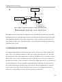
4.2.1 Object Oriented Design....................................................................................................52
5 IMPLEMENTATION AND TESTING......................................................................................55
5.1 IMPLEMENTATION ISSUES...............................................................................................55
3
5.1.1 Algorithm Complexity.....................................................................................................57
5.2 STRESS TESTING..................................................................................................................60
6 EXPERIMENTS AND RESULTS...............................................................................................63
6.1 ARTIFICIAL DATA...............................................................................................................63
6.2 REAL DATA...........................................................................................................................68
6.2.1 Triangulation....................................................................................................................69
6.2.2 Mean Curvature Threshold..............................................................................................71
6.2.3 Comparison With Other Methods ...................................................................................71
6.3 NOISE RESISTANCE............................................................................................................74
6.4 AFFINE INVARIANCE..........................................................................................................76
6.5 LIMITATIONS........................................................................................................................78
6.5.1 Cutting Planes..................................................................................................................78
6.5.2 Execution Time................................................................................................................80
7 CONCLUSION..............................................................................................................................81
7.1 SUMMARY.............................................................................................................................81
7.2 FURTHER WORK..................................................................................................................82
REFERENCES................................................................................................................................84
APPENDIX A...................................................................................................................................89
APPENDIX B...................................................................................................................................92
B.1 THE ZUCKERHUMMEL GRADIENT OPERATOR.........................................................92
B.2 3D SOBEL GRADIENT OPERATOR MASKS....................................................................92
B.3 SYSTEM AND USER MANUAL..........................................................................................93
4
1 Introduction
1 INTRODUCTION
This chapter begins with a brief background introduction on the skeleton of a shape (or object in
3D), some of the most common skeletonisation methods and popular application areas. It then goes
on to describe the main problems associated with using a skeleton in computer graphics and how
this project aims to contribute towards the solution of some of these shortcomings. Any such contri
butions and advances are briefly described here. Finally, this chapter concludes with the structure
and content of the report.
1.1 BACKGROUND
Starting with the definition of the skeleton, it can be said that a skeleton of a shape in two dimen
sions, or of an object in three, is simply the result of a skeletonisation process on this shape or ob
ject. Such a skeletonisation process is one where discrete sample points are gradually removed
from the object or shape, while preserving its continuity and connectivity, in order to generate a
more simple representation of the object or shape. There are of course alternative definitions for the
skeleton and as a result different kinds of skeletons. However, the general effects are similar as are
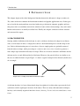
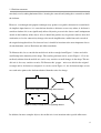
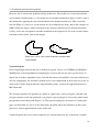
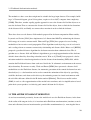
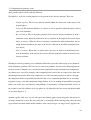
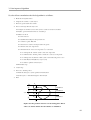
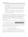
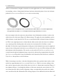
the uses to which skeletons are put. Figure 1.1 shows a typical example of the skeleton (medial axis)
of a rectangle.
Figure 1.1 A rectangle (left) and its medial axis (right)
A skeleton therefore is a lower dimensional shape description of an object that represents the local
symmetries and the topological structure of the object. There are many skeletonisation techniques,
but they can be broadly organised into three classes, thinning, Voronoi skeletons and distance trans
forms. 5
1.1 Background
Thinning, or morphological erosion, are methods based on Blum's grassfire formulation [Blu64],
[Blu73], and operate by successively eroding points from the boundary of the object, while retain
ing the end points of line segments, until no more thinning is possible. When this is accomplished,
what remains is an approximation to the skeleton. This class of operations are quite sensitive to the
most important geometrical transformations (translation, rotation and scaling) and typically cannot
localise skeletal points accurately.
Voronoi skeletons are the result of a different class of skeletonisation operations, which are based
on a special property of the Voronoi diagram. More specifically, it has been shown [Sch89] that, un
der appropriately chosen smoothness conditions and as the sampling rate increases, the vertices of
the Voronoi diagram of a set of boundary points will converge to the exact skeleton. This idea has
been used successfully [Ogn93], [SPB96] in developing skeletonisation algorithms in 2D and 3D.
This method can preserve the topology and accurately localise skeletal points but only if the bound
ary is sampled densely enough. Unfortunately, however, the practical results of Voronoi skeleton
isation methods are not invariant under Euclidean transformations and can require an additional op
timisation step, which in 3D can have a high computational complexity.
The final class of skeletonisation methods, the distance functions, are based on the fact that the
locus of the skeletal points are coincidental with the singularities (creases or curvature discontinuit
ies, also known as shocks) of a distance function to the boundary. An appropriate distance metric
(such as Euclidean, cityblock or chessboard distance) is first used to calculate the distance trans
form of the object. The local maxima of this distance function or the corresponding discontinuities
in its derivatives are then detected, each of which indicates a skeleton point. The numerical detec
tion of these singularities, however, is in itself a nontrivial problem. Whereas it may be possible to
have good localisation of the skeleton points, ensuring homotopy with the original object is diffi
cult.
In digital spaces only an approximation to the true skeleton can be extracted. Therefore, these ap
proximations need to fulfil two main requirements if they are to be considered as true approxima
tions to the skeleton. The first is topological, which is the requirement that the skeleton will retain
6
1.1 Background
the topology of the original object (i.e. properties of objects which are preserved through deforma
tions, twistings, and stretchings). The second is geometrical, which requires that the skeleton is as
thin as possible, connected, in the middle of the object and invariant under the most important geo
metrical transformations, including rotation, translation and scaling. Of course these requirements are not exhaustive and may differ for different application areas. For
example, object recognition requires thin skeletons with primitive features in order for similarity
comparisons to take place. On the other hand, skeletons with detailed geometric information are ne
cessary for surface reconstruction applications, so that the approximation error in the reconstruction
process is minimized.
There are indeed many application areas where the skeleton of an object or shape can be used. Some
of them are:
•
Fast object recognition and tracking: This is the process of determining which, if any, of
a given set of objects appear in a given image or image sequence. Since the skeleton re
tains shape information and is a reduced representation of the original shape it can be
used to match shapes/objects much faster than conventional methods, because of the few
er number of points in the skeleton. The same idea lies behind the use of feature tracking,
which is actually the correlation of an extracted object from one data set to the next. See
[Su03] and references therein.
•
Animation control: Animation usually consists of three steps: modelling, deformation and
rendering. The step of deformation for polygon based animation is carried out with the
help of skeletons. The animator moves the skeleton which in turn causes the object to de
form in the same way. See [GKS98] and [Oli03].
•
Surface reconstruction: This is an important process in geometric modelling for generat
ing piecewise smooth surfaces from data captured from real objects. A medial axis trans
form (MAT) skeleton performs well in this case because it retains all the boundary in
formation of the original object. Therefore, by applying the inverse transformation, it is
7
1.1 Background
possible to reconstruct the surface of the object. See [ACK01] and [DG03].
•
Shape abstraction: Skeletonisation from thinning gives a set of unconnected voxels,
which can then be connected into a skeleton tree. By using the distance transform values
of these voxels, it is possible to construct a graph, the minimum spanning tree (MST) of
which will automatically connect the voxels. The MST contains shape information, and is
subject to processing by standard, well known algorithms for searching, traversal and
shortest path discovery. This in itself greatly expands the use of a skeleton to several do
mains. See [GS98].
•
Text processingcharacter recognition: This is the process of identifying machine printed
and handwritten characters in an automated or a semiautomated manner. Given a charac
ter image its skeleton is extracted and then compared with a set of templates (or proto
types). See [MP90] and [AW02].
•
Automatic navigation: By using skeletonisation, the centreline of an object can be detec
ted quite accurately and then can be used as a path for camera navigation in computer
graphics and animation, or for path navigation in robotics. If the skeleton is centred, colli
sions with the object boundaries are avoided. See [WDK01].
1.2 PROBLEM STATEMENT
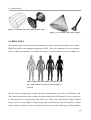
Articulation and animation of 3d human body models, such as these produced by the Body Lines
scanner [Hor95], are dependent upon an underlying skeleton, which most often requires some
manual intervention from the animator. It is possible, however, to automatically produce such skel
etons by using traditional image processing techniques (such as the medial axis transform) which
can be extended to 3d. Alternative techniques, such as principal components analysis (PCA) may be
used to detect the main limb axes and be used as a precursor to the body skeleton, with little or no
intervention. For example, Oliveira and Buxton [OB01] have approximated the medial axis of a hu
8
1.2 Problem statement
man body scan by taking horizontal slices, locating the centroid and joining these centroids to build
the skeleton.
However, even though such popular techniques may produce acceptable skeletons for certain kinds
of simplistic input datasets, it is soon obvious that these skeletons are not very robust. A skeleton is
considered robust if it is not significantly affected by noise present in the data or small, unimportant
details on the boundary of the object. Also, it should not produce any degenerate surfaces after skel
etonisation, or lead to connectivity changes after mesh simplification, subdivision and remesh of
the original triangulated data. Last but not least, it should be invariant to the most important classes
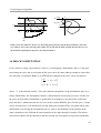
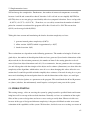
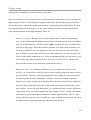
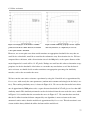
of transformation, such as Euclidean and affine transforms. To illustrate this, let us consider the medial axis of the rectangle from Figure 1.1 above and add a
small bump in the boundary of the shape. The resulting skeleton can be seen in Figure 1.2. It is im
mediately obvious that the medial axis can be very sensitive to small changes in the shape. The me
dial axis is also very sensitive to noise. To illustrate this “pepper “ noise was added to the original
rectangle and its skeleton was computed. As can be seen in Figure 1.3, the skeleton attempts to con
nect each noise point to the skeleton obtained from the noise free image.
Figure 1.2 Rectangle with small bump and its skeleton
Figure 1.3 Noisy rectangle and corresponding skeleton
In addition, for more complex objects, the medial axis is not invariant under special affine trans
9
1.2 Problem statement
formations (nonsingular linear transformations composed with translations). The PCA skeleton can
suffer similar noiserelated effects, since spurious values in the boundary may throw off the skelet
onisation process and produce limb axes that do not fall in the centre of the object. Such effects are
exaggerated by the wellknown sensitivity of least squares techniques, which PCA being equivalent
to Pearson's regression effectively, is to outliers. To overcome such problems, it is necessary to in
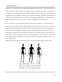
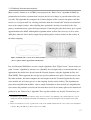
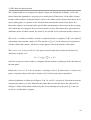
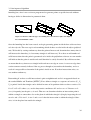
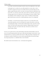
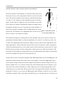
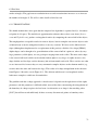
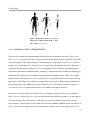
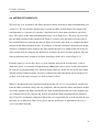
troduce additional image processing steps (such as smoothing) before skeletonisation. The same applies to 3d objects and in particular 3d body scans. In Figure 1.4, the medial axis of a
relatively noise free human body is compared with the skeletons from the same body, but with some
random surface and random volume noise added. As the illustration shows, the skeleton produced
from the body scan to which surface noise has been added (the one in the middle) will reflect the
surface noise with branches in the skeleton, resulting in a more complex structure. These effects are
more emphasised when the noise is inside the object (volume noise), where even for a small amount
of Gaussian noise the resulting skeleton can change considerably (rightmost skeleton) and even be
come discontinuous. More detailed results that demonstrate the effects of noise on medial skeletons together with Figure 1.4 Skeleton from a body scan (left) and
skeletons after addition of surface and volumetric
noise the the scan (centre and right respectively).
description of how they behave under affine transformations are presented later in this report and in
10
1.2 Problem statement
the appendices.
1.3 AIM
A solution to the problems associated with the medial axis has been proposed by Betelu et al
[Bet00] which produces affine invariant skeletons of 2d shapes that are not affected by noise. Re
cently [Bet01], this solution has been extended in 3d with promising results for simple objects al
though albeit quite time consuming, computationally expensive and numerically unstable process.
The primary aim of this project is to examine the application of this theory to human body scans
and other objects in general, and to determine if the proposed algorithm has any benefits over exist
ing popular and newly developed skeletonisation techniques. Part of this examination, will be to de
termine if and to what extent the affine invariance and noise resistance properties that worked so
well in 2d, work in 3dimensions. A secondary aim is to further improve the algorithm by reducing
its running time, but also to produce an implementation that can be used with more conventional 3d
formats, such as triangulated OFF files (3d data and connectivity information).
1.4 CONTRIBUTIONS
Perhaps the most significant contribution of this study on skeleton research, has been the use of the
3d affine invariant skeleton on models of the human body. So far, amongst its type of skeletons,
only the medial axis has been used in body scans, which as mentioned previously is not robust nor
invariant under affine transformations, unlike other onedimensional affine invariant skeletons, a
topic that will be analysed more in the next chapter.
Also, this is an important application of a theory that has been quite successful in two dimensions,
but whose extension in three is not so straightforward and has not been tested thoroughly. This pro
ject attempts to test an implementation of a specific skeletonisation process (based on 3d affine
erosion) with real and artificial input data and to determine whether it is indeed invariant to com
mon transformations, how and to what extent it is affected by noise, whether it can have the poten
tial for practical applications in object animation and how it compares with more recent advances in
the area.
11
1.4 Contributions
As far as the skeletonisation algorithm is concerned, some improvements have been implemented
and others introduced, that reduce the overall running time of the skeletonisation process and per
haps the overall quality of the end result.
1.5 CONTENT AND STRUCTURE
This report is organised into seven chapters together with the bibliography and appendices. Chapter 2 reviews the relevant literature on the subject of skeletonisation, together with any relevant
background information. More specifically, the geometric concepts of the medial axis, medial sur
face, Voronoi skeletons and the theory behind the 3d affine invariant skeleton (based on affine
erosion) is more thoroughly investigated. In addition, state of the art, alternative skeletonisation
methods and their potential uses in modelling and animation are reviewed.
Chapter 3 goes a step further and describes the algorithm behind the affine invariant skeleton the
ory, which was presented in the previous chapter. The problems and limitations of the original al
gorithm are explained together with the methods proposed for their solutions and improvements to
the algorithm, their impact on the running time, complexity and the overall quality of results. Com
putational geometry issues are also briefly included in this chapter.
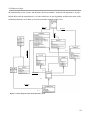
In chapter 4 the software engineering aspects of the project are presented, that is, the requirements
specification, analysis and design. Design or implementation problems are mentioned, and the way
they were solved is discussed. Furthermore, this chapter compares the different choices for al
gorithms and data structures used and the way they affected the overall quality of the results. In ad
dition, any appropriate system diagrams are included in this chapter.
Chapter 5 contains a number of software validation tests together with their results, which help es
tablish that the software is working correctly and that the algorithms are stable and efficient with
different kinds of input datasets.
Chapter 6 contains the various experiments carried out with the algorithms implemented, and the
12
1.5 Content and structure
results obtained. Both real data produced from a body scanner and artificial data where used to test
the fitness of the algorithm for creating affine invariant, noise resistant skeletons. These results are
then compared with the results of typical skeletonisation algorithms and appropriate conclusions are
drawn.
Chapter 7 summarises the research and presents the overall conclusions. Suggestions for further re
search together with theoretical and algorithmic improvements to this specific approach are dis
cussed.
Finally, we have included the appendices which contain a variety of test results and the necessary
computational geometry theory, together with the planning and execution of the project and the sig
nificance of this research. The source code of this implementation has also been included.
13
2 Literature review 2 LITERATURE REVIEW Skeletons are already widely adopted in a variety of areas. Recently, application fields such as ob
ject matching [Hil01], computer animation [WP02], collision detection and mesh editing, have
shown an increasing interest in the use of skeletons. In addition, because skeletons are better per
ceived by humans than other shape descriptions, they are best suited for humancomputer interac
tion applications.
This chapter describes both traditionally used and recently developed skeletonisation methods, their
theoretical concepts, advantages and problems, citing relevant publications as necessary. A special
type of skeleton, the affine invariant skeleton, is more closely examined and the theory behind the
algorithm used in this project is presented. Advances in the area of affine invariant skeletons, espe
cially since the implementation of this project are also included as an alternative to our chosen al
gorithm.
2.1 TRADITIONAL SKELETONISATION METHODS
Traditionally, there are two kinds of approaches to constructing the skeleton of an object. One is to
compute the skeleton directly from the object surface points, and the other to extract the skeleton by
constructing a distance field of an object. Some typical examples of both of these methods are ex
amined here.
2.1.1 DIRECT COMPUTATION METHOD
The medial axis
Perhaps the most commonly used skeleton is the medial axis, derived from Blum's original work.
Empirically, the medial axis can be thought of as a branching geometric centreline of a 2d shape. In
three dimensions, it becomes a centralised surface and the term medial surface is used instead. The
medial axis is defined as the locus of the centres of all the maximal disks, that are inside the shape
and intersect the boundary of the shape in at least two different points. Similarly, for 3d, the medial
14
2.1 Traditional skeletonisation methods
surface is the locus of the centres of the maximal spheres. Both of these concepts can be extended to
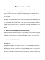
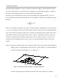
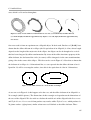
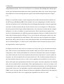
higher dimensions. Figure 2.1 shows how discrete points on the skeleton are computed via maxim
um inscribed circles, and also the medial surface in 3d (solid lines).
Figure 2.1 Left: Maximal circles interior to the rectangle with their centres. The centres are points on
the medial axis. Right: 3d medial surface of a box
Together with the medial axis, we often store the radii of the maximal disks (or spheres). The idea
behind this, is that we can use this extra information to reconstruct the original object. The medial
axis in conjunction with this distance function defines the medial axis transform (MAT). The ob
ject's boundary and its MAT are equivalent, and one can be computed from the other. Usually, a 2
dimensional shape will be transformed into a 1dimensional structure, while a 3dimensional object
will be transformed into a 2d surface. The medial axis has been studied extensively, especially as a means for shape representation
[NP85], [WOL92], object decomposition for mesh generation [She96], shape morphing and anima
tion [Teic98] and motion planning [Wil99]. This theory however, is not without problems. We have
briefly seen in the introduction, how the MAT produced undesirable skeleton branches when the
curvature of the object surface varies everywhere (noisy surface). Since this is a morphologically
meaningless property of the MAT, some studies have focused on the simplification of a noisy MAT
by means of pruning [SB98],[Ogn95].
15
2.1 Traditional skeletonisation methods
However, this is not the only problem with the medial axis. The medial axis is not invariant under
special affine transformations (i.e. the medial axis of an affinetransformed shape is not the same as
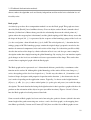
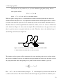
that obtained by applying the same transformation to the original medial axis). This is best illus
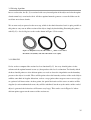
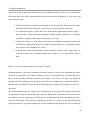
trated in Figure 2.2, where we see the medial axis of an elliptical pie shape, akin to the examples in
[JB01]. When the shape is affinetransformed, the calculated medial axis has additional branches.
Clearly, it does not correspond to an affinetransform of the original axis. We will revisit the affine
transform in more detail, later in this chapter.
Figure 2.2 A concave curve and its medial axis, and after affine
transformation
Voronoi diagram
Exact computation of the medial axis is difficult in general. Culver et al. [CKM99] and Hoffman
[Hof90] have created algorithms for computing the exact medial axis for some special classes of
shapes but even these algorithms had to deal with the numerical instabilities associated with the me
dial axis computation. An alternative method for the exact computation of the medial axis is the cre
ation of the Voronoi diagram from the shape boundary points, and then the approximation of the
MAT from that.
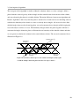
The Voronoi diagram is the partition of n points in a plane into n convex polygons such that each
polygon contains exactly one point and every point in a given polygon is closer to the point in that
polygon than to any other point (Figure 2.3). The generated polygons are known as Voronoi poly
gons, and from what we can see in the illustration, the points where the boundaries of these poly
gons meet, form an approximation to the medial axis.
Voronoi diagrams have been widely adopted in the construction of 2d and 3d skeletons [Ogn92].
16
2.1 Traditional skeletonisation methods
More recently, Amenta et al. [ACK01], have proposed the “Power Crust” algorithm for MAT ap
proximation and surface reconstruction, based on the idea of shapes (a generalisation of the con
vex hull). The algorithm first computes the Voronoi diagram of the scattered data points, and then
retrieves a set of polar balls1 by selecting candidates from the Voronoi balls2 that have maximal dis
tance to the sampled surface. After labelling these polar balls, the object described by the data
points is transformed into a polar ball representation. Connecting the polar ball centres gives a good
approximation to the MAT. Although this algorithm works well on dense data sets, it faces some
difficulties when the data is under sampled by producing holes or other artefacts in the vicinity of
the undersampling. Figure 2.3 On the left a convex curve and its medial axis, and on the right the Voronoi diagram of the
curve, together with its approximated medial axis.
Dey and Goswami [DG03]have created a simple algorithm called “Tight Cocone” (based on the ori
ginal “Cocone” algorithm by Amenta et al. [Ame02]) for watertight surface reconstruction that can
approximate the medial axis directly from the Voronoi diagram, using the algorithm by Dey and
Zhao [DZ02]. Their approach does not pay any special attention to the poles (Voronoi vertices) un
like other methods, but rather computes the subcomplex from the Voronoi diagram that lies close
to the medial axis and converges to it as the sampling density reaches infinity. The algorithm em
ploys mesh simplification methods, such as sample decimation or direct medial axis simplification,
to overcome the problems caused by the fact that there tend to be too many spikes in the medial axis
produced by the “Power Crust” algorithm. This, together with the way that the Voronoi facets are
1 The MAT is approximated by a subset V of the Voronoi vertices of S, called the poles, which (where S is a good
sample) lie near the medial axis. The balls surrounding the poles and touching the nearest samples are the polar
balls.
2 The Voronoi balls for a a set S of points in R³ , is the set B of balls centred at the Voronoi vertices of S such that B
= Vor(S). The polar balls are a subset of the Voronoi balls .
17
2.1 Traditional skeletonisation methods
chosen, makes the algorithm scale and density independent and the medial axis calculation less af
fected by noise.
Reeb graph
A relatively uptodate direct computation method is to use the Reeb graph. This graph was intro
duced by Reeb [Ree46], based on Morse theory. Given an object surface M and a smooth valued
function ƒ defined on it, Morse theory provides the relationship between the critical points of ƒ
(points where the tangent plane is horizontal) and the global topology of M. Morse theory states that
the shape of the pair (M, ƒ) is represented by the sequence of the homology groups of the level sets
(i.e. the set of points x from M such that ƒ(x)<k, k∈ℝ. The critical points of ƒ determine the ho
mology groups of M. The homology groups contain the original shape's properties encoded as the
number of connected components, holes and cavities of the shape. Its is therefore possible to fully
describe the surface of the shape by a finite collection of levelsets, and also get a more complete
description rather than simply knowing the global homology. By varying k we can introduce topolo
gical changes on the levelsets and obtain a discrete representation of the shape. This can be then
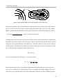
encoded into a topological graph called the Reeb graph. The Reeb graph can be represented as a 1dimensional skeleton, provided by a continuous scalar
function on the surface M. Although the global homology of the surface M does not change as ƒ
varies, the topology of the levelsets depends on ƒ. In this way, the choice of ƒ determines a col
lection of shape descriptors with properties dependent on the function ƒ that characterise the ob
ject's surface depending on the application context. Typically, f is chosen as the height function
(∀p=(x,y,z) ∈ℝ3, f(x,y,z)=z) whose critical points (i.e. peaks, pits and passes) are useful for shape
description. The main drawback of using the height function is that it produces graphs which are de
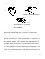
pendent on the orientation of the object in space (not affine invariant). Figures 2.4 and 2.5 show
how the Reeb graphs of real and generated data look.
Some research on Reeb graphs, has been carried out using the geodesic distance (which is the min
imum length of the paths connecting two vertices u and v of a finite graph ) as the mapping func
tion. More specifically, Lazarus and Verroust [LV99], have used the idea of Reeb graphs to con
18
2.1 Traditional skeletonisation methods
struct a skeleton called the LevelSet Diagram, in which the geodesic distance from a source point is
used as the function h. Their solution however, is dependent on the choice of source points, and for
that reason it is not unique. Different LevelSet Diagrams can be produced for the same model. Hil
aga et al. [Hil01], have defined the Multiresolutional Reeb Graph based on the geodesic distance,
and used it as a search key for topology matching. The have developed a series of Reeb graphs for
an object at various level of details, partitioning the object into regions using the height function at
every level.
Figure 2.4 Reeb skeleton (bold) of real
3d data (only the boundary of the object
is shown here for simplicity)
Figure 2.5 Reeb graph of a torus (bold lines).
The graph will correspond to the topology of
the object. The skeleton produced by the Reed graph has some interesting properties that make is especially
useful as an object recognition and matching key. Firstly, a Reeb graph will always be a 1dimen
sional graph structure and will never have any higherdimensional components such as degenerate
surfaces. Secondly, by correct choice of the continuous function f, it is possible to obtain a Reeb
graph that is invariant to translations, rotations and connectivity changes that occur from simplifica
tion, subdivision and remesh. The remeshing property also helps to ensure that such a Reeb graph
is quite resistant to noise.
2.1.2 DISTANCE FIELD METHOD 19
2.1 Traditional skeletonisation methods
The methods we have seen above might not be suitable for large input datasets. For example, build
ing a 3d Voronoi diagram, given N data points, requires at least O(N2) computer time complexity
[GN00]. Therefore, another equally popular approach is to use the distance field of the object to ex
tract the skeleton. First we construct the distance field of the object, then we find the local maxima
of the distance field, and finally we connect these maxima in order to find the skeleton.
There have been several distance field methods proposed for skeleton computation. Most notably,
Leymarie and Levine [LL92] have implemented a 2dimensional MAT by minimising the distance
field energy of an active contour model. Zhou and Toga [ZT99] have proposed a voxelcoding
method based on recursive voxel propagation. Their algorithm works by using a set of seed voxels
and a coding scheme to construct connectivity relationship and distance fields. Bitter et al. [BKS01]
proposed a penalizeddistance algorithm for skeleton extraction from volumetric data. The al
gorithm uses a distance field and Dijkstra's algorithm to get a rough approximation of the skeleton,
which is then refined by discarding redundant voxels. Wan et al. [Wan01] have proposed a skelet
onisation method for virtual navigation based on the distance from boundary (DFB) field, which
contains the Euclidean distance from each voxel inside the 3d volumetric environment to the nearest
object boundary. Even more recently, Wade and Parent [WP02] have presented a distance field
method that uses the Euclidean distance, for automatic generation of the control skeleton of an artic
ulated object (i.e. a skeleton that can be used to control the animation of the object by specifying
sticklike skeletons, and often used in this way for animating avatars in virtual environments with
the stick like skeletons defined in the HAnim standard [HAnim]). The discrete medial surface
(DMS) is used as a first approximation of the medial axis transform, and via simplification of voxel
paths their system produces a relatively good control skeleton for 3d objects.
2.2 THE AFFINE INVARIANT SKELETON
As we have mentioned previously, because the medial axis uses the Euclidean distance, in the form
of the radius of bitangent circles, it is invariant under Euclidean transformations (rotations, transla
tions and reflexions) but not invariant under special affine transformations (i.e. nonsingular linear
20
2.2 The affine invariant skeleton
transformations composed with translations). Therefore, we can define an affine invariant skeleton
as being invariant under the special affine transformation
X'=AX+T
where X,X' and T are vectors and A is a 2x2 matrix (or 3x3 in the case of 3d skeletons). The trans
formation is volume and orientation preserving with determinant equal to 1 rather than 1. In prac
tical terms, this means that if a shape is deformed by such an affine transformation, and then its
skeleton is computed, that skeleton should be the same as the skeleton computed from the original
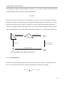
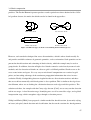
shape and transformed via the same affine transformation. Figure 2.6 is an illustration of this idea.
Affine transform
Skeletonise
Skeletonise
These skeletons must be the same
Affine transform
Figure 2.6 Definition of the affine invariant skeleton
2.2.1 IN 2 DIMENSIONS In [SG98], Giblin and Sapiro defined the affine distance between a point x and a point C(s) on a
curve, as the area between the curve and the chord from C(s) that passes through x:
C s
1
d x , s= ∫ C−x × dC
2 C s '
21
2.2 The affine invariant skeleton
where × is the z component of the cross product of two vectors, and C(s) and C(s') are the points in
the curve that define the chord, which contains x. This can be seen in Figure 2.7. C(s)
X
C(s')
Figure 2.7 Affine distance of a closed
Figure 2.8 Affine skeleton of concave curve and after affine
curve
transformation
From here onwards, the definition of the skeleton is similar to that of the medial axis. Thus, a point
x is said to be on the affine invariant skeleton if and only if there exist two different points C(s1)
and C(s2) which define two different chords that contain x and have equal areas d(x,s1)=d(x,s2),
provided that these distances are defined and they are global minimum. If the distances are just local
extrema, point X is said to be on the affine area symmetry sets of the curve. This definition of the
skeleton is more resistant to noise than the MAT because the computation of the area averages out
noise to some extent. Betelu et al. [Bet00] have proposed a numerical implementation of the affine
skeleton, the results of which we can see in Figure 2.8. Note that it deforms correctly under affine
transformation, unlike the MAT from Figure 2.2 above.
In the same publication, Betelu et al. have defined the affine erosion E(C,A) of a convex curve C as
the set of points x of the interior of C that satisfy E(C,A) := {x ℝ2 : ƒ(x)≥A≥0}
where ƒ(x) is the minimum distance from a point x to the curve f x =inf {d x , s s ∈ D} , where
D is the domain of d(x,s) for a fixed value of x. For a specific ƒ(x)=A, we can get the eroded curve
C(A) which is the boundary of the affine erosion. C(A) := {x ℝ2 : ƒ(x)=A}
If we now consider the area A to be a time parameter, ƒ(x) represents the time the eroded curve takes
22
2.2 The affine invariant skeleton
to reach the point x. When A=0 we have the original curve, and as A increases we get the eroded
curve which is inside the original.
There is a close relationship between the affine erosion of a curve and the skeleton, more specific
ally, a shock point (point of singularity) on the erosion is a skeleton point. This is easy to under
stand for example for the affine skeleton, if you consider that a shock point x is a point on the
eroded curve where two different chords (C(s1), C(s'1)) and (C(s2), C(s'2)) of equal area A intersect.
x will be equidistant from the curve with d(x,s1)=d(x,s2), since the two chords cut equal area, but
also the distance will be a global minimum at s1. This is because x belongs to the eroded curve C(A)
and so by the definitions of C(A) and f(x) above, f(x)=inf{d(x,s), s ∈D} = A. This ensures that the
shock point x is on the affine skeleton.
Recently, Estrozi, Costa and Giblin [LCG03] in order to tackle the affine skeleton for nonconvex
curves have used polar coordinates to define the curve and redefined the chordal area as 1
A=
2
∫ r2 d
where is the angle of the chord and r=r() is the polar equation of the curve. The skeleton defined
this way may produce disconnected axes owing
to inflexions in the curve.
2.2.2 IN 3 DIMENSIONS
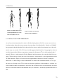
There has been an attempt to approximate the 3d affine skeleton by M.S.Jeong and B.Buxton
[JB01] in 3d human body scans. Their approach was to calculate the affine skeleton for 2d horizont
al crosssections of the body and then from that create the affine skeleton. Their preliminary results
have shown that the produced skeleton is less sensitive to noise than the medial axis, and seems to
deformed appropriately under linear transformations.
23
2.2 The affine invariant skeleton
The 3dimensional case was proposed by Betelu, Sapiro and Tennebaum in [Bet01], and it is the
theory behind the algorithm we are going to use in this project. Extended to 3d, the affine distance
becomes affine volume (or chordal volume), and it is the volume enclosed between the object and a
chord (cutting plane) at a point X, in the direction outwards from the interior of the object. It is
known that volumes are invariant under special affine transformation, and because of the averaging
effect when they are computed, they are also insensitive to noise. The authors have given three key
definitions for the 3d affine erosion, the chord set, the erosion levelset function and the erosionset.
The chord set is defined as follows: Assume a volume (bounded set of points) V⊂ℝ3, and a plane ∏
with normal n that contains a point x∈V. The chordal set ∑(x,n,V) is the connected set of points in
side the volume that contain x and that are on the opposite side of the normal n of the plane.
The erosion levelset function E(x,V) is the greatest lower bound of the volume of all chord sets
defined by all points x∈V. E x , V =inf v ∑ x , n , V
n∈S
where the inf (greatest lower bound) is computed with the normals n pointing at all the directions of
the unit sphere.
Finally, the erosionset v is the set of points x satisfying vE(x,V). In other words, we remove any
points x from the volume of the object, that have E(x,V) below some chosen threshold v.
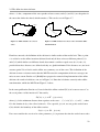
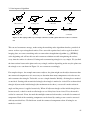
All three definitions are illustrated in Figures 2.10, 2.9, and 2.11 respectively. Note that because the
volume of the chord set is only defined for the points that are inside the object and connected to x,
in Figure 2.10 the small volume (indicated by the arrow) although cut by the plane ∏, is not con
nected to x and therefore is ignored.
24
2.2 The affine invariant skeleton
Ignored volume
(x,n,V)
∏1
∏2
∑(x,n2)
∏
x
x
n
∑(x,n1)
n2
n1
Figure 2.9 The erosion levelset function, will be the
Figure 2.10 The chordal set (shaded) at point x
smallest chordal set at point x
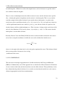
E(x',V)<v
x'
E(x',V)>v
E(x',V)=v
Figure 2.11 The erosion set v is the set of all the
points where the erosion levelset function E(x,V) is
above a certain threshold.
So, in this case and in an analogous way to the 2d case, the 3d affine invariant skeleton is defined as
the shocks (or the discontinuities on the normals of the erosion set) of the contour surfaces E(x,V)=const (corners of erosion sets).
According to Betelu et al. [Bet01], the results from the 3d affine erosion seem quite robust even for
objects with complex topologies (e.g. with holes). The approximation of the skeleton however, has
proven to be a rather more problematic goal to achieve, owing to the inherent difficulty in comput
ing the shock points. Furthermore, because we are now not dealing with Euclidean distances but
with volumes, which are slower to compute, the overall computation of the erosion is affected.
More specifically, with implementation proposed by Betelu et al. it was estimated that the erosion is
O(N5/3), where N is the number of voxels in the volume. The bulk of the computation time is spend
on computing the erosion levelset function for the volume, and in the next chapter we discuss some
ways that we can reduce the running time of the algorithm, and also some ideas on how to deal with
the shock computation.
25
2.2 The affine invariant skeleton
2.3 RECENT SKELETONISATION METHODS
Since the beginning of this project, there have been a few interesting advances in the area of skelet
onisation and affine skeletons and it seems that there is particular interest in the study of thin, tree
structured 1dimensional skeletons for use in object recognition or animation, in distinction to the
2d surface like skeletons such as the affine skeleton and the medial axis in 3d.
Perhaps the most significant development in the area of affine invariant skeletons is that of Mortara
and Patané [MP02] who they have extended the theory of Reeb graphs to produce 1d affine invari
ant skeletons. Even though many extensions to the Morse theory have been proposed, the Reeb
graph suffers of at least two problems. First it depends on the choice of function ƒ and second there
is no distinction between small and large features of the shape, owing to the fact that connected
components are collapsed into the same class without any distinction of their sizes. Furthremore, as
we have already noted, Mortara and Patané argue that the choice of the height function as the gener
ic function for constructing the Reeb graph, will produce graphs that are dependent on the orienta
tion of the object in space. They propose a definition of the Reeb graph using topological distance
from global features, defined by source points in high curvature regions to guarantee that the result
is affine invariant, and therefore, not dependent on the orientation of the object in space. Compared
with skeletons produced by using the height function, their approach is affine invariant because the
chosen function ƒ does not rely on either the coordinate system nor on the surface embeddings.
However, if the curvature evaluation process, which is an intrinsic step of their algorithm, does not
recognise at least one feature region, their approach is not useful for extracting a description of the
shape. On the contrary, the height function always guarantees a result.
Even more recent publications are those from WC Ma et al. [MWO03] and [Wu03]. In the first,
the authors attempt to extract the skeleton from 3d objects by building its distance field by using
Radial Basis Functions (RBFs). They then apply a gradient descent algorithm to locate the local ex
trema in the RBFs which indicate branching or termination nodes of the skeleton. RBFs are continu
ous functions which is a good property for use in gradient descent, but construction of an appropri
ate RBF which preserves the geometrical properties of arbitrary 3d models is still under considera
26
2.3 Recent skeletonisation methods
tion. In their second publication [Wu03], they use a different approach, based on what they call the Vis
ible Repulsive Force (VRF) to locate local extrema. The author provide three definitions. The first is the visible set V(x). Assume a point x in the interior of a surface S, so V(x)={vi | vi x, vi ∈ S} (ab denotes that a is visible to point b). Then the VRF is defined as:
VRF x =∑ f ∥v i −x∥⋅
v i −x
where vi∈V(x) and f(r)=r2 is used as as the Newtonian potential function.
Finally, they define the Visual Domain Skeleton (VDS) of the object as D(S)=(Q,M)
where Q represents the set of local minima in VRF, and M an operator used to describe the topolo
gical relationship in Q. The local minima of VRF are located by first using a radial parametrisation
process and then a shrinking procedure. The authors name each of the local minima as VDS nodes,
and have determined that each point on the surface S will converge to a VDS node. Connecting
these nodes based on their neighbourhood relationship on the surface, will produce the skeleton. Al
though the skeleton produced has both topological and morphological information of the shape, the
skeletonisation process is not fully automated, since undesirable connections need to be removed by
hand. Furthermore, locating the VRF minima takes 95% of the execution time and for large models
it can prove rather a computationally expensive process.
27
3 Skeletonisation algorithm
3 SKELETONISATION ALGORITHM
Now that we have covered the theory behind the 3d affine invariant skeleton we will see how it can
be implemented in discrete mathematics. This of course presents its own problems since as we will
see, even simple arithmetic operations can have many pitfalls when implemented on a floatingpoint
computer system. In this chapter we briefly describe such computational geometry issues and exam
ine the 3d affine erosion algorithm more closely. Problems associated with this algorithm, such as
speed and accuracy, and what causes them are identified, and addressed in the section algorithm im
provements. Finally, we conclude with a discussion on the issues of computing shock points.
3.1 COMPUTATIONAL GEOMETRY ISSUES
In previous chapters we have seen the theory behind the medial axis construction and other skelet
onisation methods, given in the context of continuous geometry. In continuous geometry, an object
is defined using a continuous representation, usually as a polygon, polyhedron or some closed curve
or surface. Skeletons such as the medial axis and Voronoi graphs are defined using curves, surfaces
or continuous approximations of them (e.g. with polygonal meshes).
When the same ideas are applied in computational geometry, there are more approximations in
volved. An object analytically defined in continuous space, will need to be approximated as a set of
discrete points in a rectilinear grid, and in a Cartesian coordinate system. In 2d, the object is said to
be pixelised, whereas in 3d it is said to be voxelised.
The skeleton of the object must be approximated as well, and typically, it will be a subset of the
points of the discrete object, if we consider the object as a volume and not only as a boundary. The
mathematical definition of the skeleton results in a computation of a unique skeleton for any given
object. In the discrete case however, there are different approximation methods for constructing the
skeleton, and since there is no uniform mathematical definition, there can be noticeable differences
between the skeleton of the same object constructed with different algorithms. In addition, whereas
the continuous skeleton has the same topological structure as the continuous object, there is no
guarantee that the discrete skeleton will preserve the topology of the discrete object. In fact, it is
28
3.1 Computational geometry issues
quite possible that it will be radically different. Nevertheless, we desire certain properties to be present in the discrete skeleton. These are:
•
Similar topology: The discrete skeleton should exhibit the same basic connectivity as the
original object. •
Centered: The skeleton should be as centred as well as possible within the object, with re
spect to its boundary.
•
Reconstruction: The set of points generated by the inverse distance transform (if such a
transform exists) should be identical to the set of points of the original discretised object.
•
Affine invariance: When the discrete skeleton is submitted to affine deformation, the res
ulting skeleton should be the same as the discrete skeleton of the affine transformed dis
crete object.
•
Noise resistance: When there is surface noise (presence or absence of individual pixels
near the boundary of the object) the discrete skeleton should be similar to the noisefree
discrete skeleton.
Working in discrete geometry poses additional difficulties especially when trying to use formulas
from continuous geometry. We have faced a variety of problems, because of the floatingpoint nu
merical system a computer uses, and the fact that computation results and numerical comparisons
are almost never exact. For example, when comparing two vertices that we expect to be equal but
which might for instance have been computed as a result of an intersection or a split of a triangle,
the comparison will most probably fail. Besides that, every computing platform has its own float
ingpoint system, a fact that complicates things further, if we are looking for portability across plat
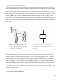
forms. One of the ways to counteract such problems is to introduce a distance threshold, and see if
the second vertex falls within a circle (or sphere in 3d) defined by the first vertex and the threshold
as its radius (Figure 3.1). Another equally valid way, is to try and bypass the floatingpoint system altogether and convert to
an integer numerical system. The way to do that, is to multiply all the floatingpoint values by an in
teger constant and then roundoff the numbers at the closest integer. As long as this is applied con
29
3.1 Computational geometry issues
sistently throughout, we should be able to avoid most of the problems associated with floatingpoint
numbers in computational geometry.
d
V0
V1 = V0
d'
V2 ≠ V0
Figure 3.1 Comparing vertices with a threshold. If d ≤ r then V0=V1
Most geometric algorithms are formulated in terms of real numbers, and the problem when trying to
implement algorithms in a floatingpoint system, is the fact that not all real numbers can be repres
ented as floatingpoint numbers. If we assume that r ∈ℝ and f(r) is its floatingpoint representation,
and in order to get from a real number to a floatingpoint r has been truncated or roundedoff to the
nearest floatingpoint, the absolute roundoff error will be ∣ f r −r∣ .
Arithmetic operators such as addition and multiplication when carried out on floatingpoint num
bers can also introduce numerical errors that will not appear in real number operations. For ex
ample, if r,s ∈ℝ and s ≠ 0, then r+s≠r. However, it is possible that f(r)+f(s)=f(r) when f(r) is
much larger than f(s). Even the properties of addition such as commutativity and associativity can
be affected when dealing with floatingpoint numbers. It is not always true for example that
f r f s f t = f r f s f t
If f(r) is much larger in magnitude than f(s) and f(t), it is possible that f(r)+f(s)=f(r) and
f(r)+f(t)=f(r). Then, f r f s f t = f r f t = f r
which is obviously not equal to f r f s f t .
There are many examples like the above, so it is essential not to rely only on mathematical logic
when implementing an algorithm. That is why many times the algorithm might appear to be radic
ally different from the actual mathematical theory on which it is based.
30
3.1 Computational geometry issues
3.2 EXISTING ALGORITHM
The algorithm proposed by Betelu et al. based on the theory we have seen in the previous chapter,
has two distinct parts. The first is the erosion of the object and the second the computation of the
shock points, or more precisely, first the computation of the erosion levelset function for every
point x' in the volume, and second the computation of the discontinuities on the normals of the sur
faces where E(x,V)=constant. We will attempt to describe these two operations distinctly, since it is
more efficient to implement and execute them separately from each other. The first operation will
erode the object and the second will detect the singularities of the eroded volume.
3.2.1 EROSION
Erosion is a fundamental operation in mathematical morphology, based on Minkowski's subtraction,
where the structuring element is a circle (or sphere in the 3d case). However, the affine erosion has
a completely different definition, with the majority of the execution involving computation of
chordal volumes.
Once we have computed the erosion levelset function E(x,V) for every point inside the volume, the
erosion step will be finished, and in principle this could be achieved by computing the volumes of
all the chord sets ∑(x,n,V) for every x∈V in all possible directions n on the unit sphere and taking
the minimum, just as in the 2d case already defined by Betelu et al. [Bet00] This solution of course,
is far from ideal and not very feasible. The number of points in the volume is very large and, when
multiplied by the number of possible orientations n we could choose, makes this approach very
computationally expensive from a practical point of view. So, Betelu et al. proposed triangulating
the surface of the object and using the inwardspointing normals of the triangles as possible orienta
tions for computing the volumes of ∑(x,n,V). This together with the fact that the volume of a chord
∑(x,n,V) is the same for all the points lying on the same plane can simplify the computation pro
cess.
31
3.2 Existing algorithm
The input to their algorithm is a surface enclosing a connected volume V, given implicitly in terms
of a levelset function F(x), and discretised in a volumetric array. This kind of surface, is similar to
the surface representation of objects used for medical image applications.
The first step is to triangulate the surface using the marching cubes algorithm [LC87]. Once we
have a polyhedral representation of the object, we can compute its volume using a boundary integral
formula:
n
v 0≈
1
∑ xi⋅ S i
3 i=1
where n is the number of triangles, Si is the area of the triangle Ti multiplied by its inwards normal
ni and xi is the triangle's centre of mass. The volume calculated in this way is just an approximation
to the actual volume of the object obtained by “breaking” the polyhedral representation of the object
with tetrahedra with bases the triangles of the object's surface , computing the volumes of these tet
rahedra, and summing them. The more triangles there are in the object's surface (i.e. the finer the
resolution of the triangulation of the surface), the closest the approximation will be to the actual
volume.
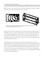
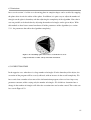
Now we can start an iteration, and for every triangle Ti on the surface of the object do the following:
•
Define a plane that contains the centre of mass xi of the triangle Ti , with normal that of
the inwards normal of the triangle n=- ni (Figure 3.2). Centre of mass xi
Triangle Ti
∏0
Plane normal n∏
Figure 3.2 Starting point of the algorithm, creating the cutting plane
•
Advance this plane along its normal towards the inside of the volume, by a distance
32
3.2 Existing algorithm
d=min(x,y, z), where x,y, z is the volumetric grid point spacing. The ad
vanced plane will be:
' ⇒ x−x il ⋅ni =0
where x li =x i ni l d and l is an iteration counter.
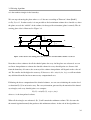
While the plane is being moved, we should find the connected chordal points that are inside the
volume and under the plane. It is very important to mention that the chordal points must be connec
ted with xi and inside the object or else the volume they enclose is not defined. What this means is,
that there must be a connected path inside the volume to connect x and x' if x' is to be a member of a
valid chordal set. Figure 3.3 shows such an example. The valid chordal set is the greyed area, since
there is a path to connect every point inside the set with x. Therefore, there is the additional step of
determining such connected components.
x
∏
x''
x'
Figure 3.3 Connected components example. x' is connected with x, unlike
x'' which is inside the volume but not connected with x.
The boundary of these points will be triangulated (by using marching cubes again) and the volume
they enclose computed by means of a boundary integral formula like before, only this time its is for
an open polyhedron, where the opening face is planar. So the enclosed volume is given by: m
1
v ≈ ∑ x k −x il ⋅ S bk
3 k=1
l
Here S bk is the area of the boundary triangles T bk each multiplied by their inwards normal and
xk is their centre of mass. The letter b indicates that the triangles are part of the new boundary, and
33
3.2 Existing algorithm
m is the number triangles in the boundary.
We can stop advancing the plane when vi≥v0/2 because according to Theorem 3 from [Bet01],
0≤E(x,V)≤v0/2 . In other words, it is not possible to find a minimum volume for a chordal set, when
the plane exceeds the “middle” of the volume, for that specific orientation (plane's normal). The ad
vancing plane idea is illustrated in Figure 3.4.
xi
d
xi1
d
0
}v
1
xi2
}v
2
1
2
v0 / 2
Figure 3.4 We advance the cutting plane and calculate the chordal volumes until we reach v0/2
Now that we have volumes for all the chordal points for every d the plane was advanced, we can
use linear interpolation to estimate the chordal volume for every chordal point at a distance ld
from the boundary. Of course, the accuracy of the volume interpolation will depend on the value of
d. The smaller d the higher the accuracy. If, however, d < min(x,y, z), we will not obtain
any additional benefits but incur unnecessary computational cost.
Following the above computation of the chordal volumes, we can start calculating the erosion level
set function E(x,V) in an iterative way. For every orientation generated by the normals of the bound
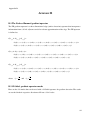
ary triangles, and every chordal point x we compute:
E(x,V) = min(E(x,V), uint((xxi)•ni))
where uint is the interpolated volume.
When all the triangles are exhausted, E(x,V) will contain the minimum volume. We also store the
the normal (optimal normal) that produces this minimum volume. At the end of the algorithm, we
34
3.2 Existing algorithm
have a scalar value, the E(x,V), associated with every internal point of the object and also the optim
al unit normal n(x) associated with it. All these optimal normals generate a vector field that can be
used later on to detect shocks.
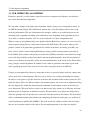
We are now ready to proceed to the next step, which is the shock detection, but it is quite possible at
this point to carry out an affine erosion of the object simply by thresholding. Retaining the points x
with E(x,V) > threshold gives us the results shown in Figure 3.5 for a torus:
Figure 3.5 Original torus (left) with volume v0 , affine erosion with a
threshold v0/10 (middle) and with a threshold of v0/7 (right).
3.2.2 SHOCKS
So far, we have computed the erosion levelset function E(x,V) for every chordal point x in the
volume and the optimal normal vector n(x) that produces this levelset function. To identify which
of these chordal points are also skeleton points, we need to detect the singularities on the boundary
present as the object is eroded. These will be points where the boundary surface of the eroded object
exhibits some kind of singular behaviour, such as a cusp (point where tangent vector reverses sign)
or a point of selfintersection. At these points, the partial derivatives of the curve or surface will be
singular (in strict mathematical terms, they will be undefined, but the way the surface of the eroded
object is generated the derivatives will become very large). This can be seen in Figure 3.6 where
skeleton points appear on the corners of the erosion sets.
35
3.2 Existing algorithm
Shock points
Figure 3.6 Shock points (thick dots) generated from the erosion of the curve
Detecting such points can be accomplished by computing the mean curvature H(x) of the surfaces
E(x,V)=constant as the object erodes, and by keeping those where ∣H(x)∣>threshold. The authors
[Bet01], propose that the threshold is of the order of the inverse of the discretisation size. That is,
threshold=
where is of the order of unity.
min x , y , z
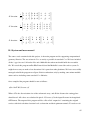
Computing the mean curvature for the surface from the surface of the eroded object is troublesome. Fortunately, the mean curvature is the divergence of the vector field of the optimal normals, and the
divergence can be approximated by finite differences. The finite difference is the discrete analogue
of the derivative (an infinitesimal change in the function with respect to whatever parameter it may
have). The divergence computed by finite differences is:
H(x) =∇.n(x)
where in 3 dimensions, the divergence is, in Cartesian form:
∇ . n x =
n x n y nz
,
,
x y z
Each of the partial derivatives may then be approximated by finite differences in the usual way
since n(x) is available over a regular grid of vectors. According to the authors [Bet01], the easiest
and fastest way to calculate them is to use the intermediate difference operator. With this operator,
36
3.2 Existing algorithm
for each axis we look at the neighbour and the optimal normal of the current voxel, thus giving us a
total of two voxels from which to sample. So, for the xaxis the operator is:
nx
x
=
n x x x−n x x
x
and can be extended in the y and z axes in a similar way. There other operators that can be used that
sample from a bigger neighbourhood and thus produce better results, such as the central difference
operator nx
x
=
n x x x−n x x− x
2x
where we look at the two neighbours at each direction
and ignore the value at the current voxel. Therefore we sample from six neighbouring voxels. Other
operators, such as the 3d Sobel, Prewitt and Zucker and Hummel, sample from even larger neigh
bourhoods, producing better results but have a slightly higher execution speed3. We will examine
such operators later on this chapter.
In conclusion, these are the two steps necessary for computing the skeleton. However, there are two
important drawbacks of this algorithm that can affect the computation of the 3d affine skeleton. The
first is associated with the erosion and its computational complexity. According to the authors
[Bet01], the algorithm is of O(N5/3) with computation time being distributed as: triangulation of the
boundary of the chord sets by means of the marching cubes algorithm 33%, connected components
53%, and computation of chordal volumes 14%.
The second problem is associated with the calculation of the shocks and concerns accurate computa
tion of the divergence. It is quite difficult to accurately isolate shock points by using a discrete ap
proximation of the mean curvature. This is because sometimes discretisation effects can lead to very
high value of the derivative estimates with the result that points can be mistakenly chosen as points
of high curvature and thus as skeleton points. In the next sections we look at some alternative ways
of alleviating some of these problems, and improving the algorithm.
3 For example the central difference operator is four times faster than the ZuckerHummel or Sobel 3D.
37
3.3 Our improved algorithm
3.3 OUR IMPROVED ALGORITHM
From here onwards, we will examine some ideas on how to improve the efficiency and effective
ness of the skeletonisation algorithm.
We start with a change to the input to the algorithm, which is going to be a triangulated surface in
an OFF file format [Geom]. The OFF format contains the vertex data followed by the faces (con
nectivity) information. This precalculation of the triangles, enables us to avoid having to use the
marching cubes algorithm. Avoiding such calculations at the beginning of the algorithm and also
every time we advance the plane, will save us an estimated 33% of the computation time
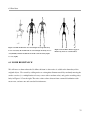
When it comes to using human body scans produced by the Body Line scanner, it is necessary to do
some preprocessing before we could convert them to the OFF format. The scanner software will
produce a cloud of 3d points that approximate the surface of the body. According to [OJ03], any
noisy vertices will be removed through filtering by using a model cleaning software provided by
Laura Dekker. This software will produce inventor files [SGIInv] with either a hierarchical or single
mesh, with the possibility of there being holes and nonmanifold portions. Joao Oliveira produced
software to read these inventor files, delete any nonmanifold parts of the mesh, and to fill the holes
using a simple centroid algorithm. In addition, Joao's software performs some minor repair work
such as pushing out dents in the arms and so on, before saving the mesh in an OFF file.
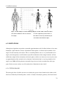
Using a pretriangulated file however, means that we have to generate points inside the volume that
will be used later as chordal points. The best way to do this is by creating a bounding box around
the object, create points at specific intervals in the box and determine which of these points are also
inside the object. There are different choices for bounding boxes, the easiest one to implement being
the axisaligned box, which has dimensions the minimum and maximum vertices of the object in
every dimension. This may however enclose an unnecessary large volume so if efficiency and com
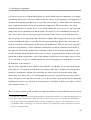
putation speed are important, it should be avoided. The next choice is an objectaxisaligned box,
where the principal axes of the object are used to fit a box that encloses the volume. The best choice
will be a minimum bounding box obtained by computing the diameter of the point set, such that de
scribed by Barequet and HarPeled [BP01]. This will enclose the smallest volume and so will pro
duce the fewest points outside of the object. For our implementation we used the axis aligned
38
3.3 Our improved algorithm
bounding box, since it was easiest to program and to generate points at specific intervals without
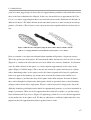
having to define its dimensions in parametric form.
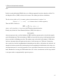
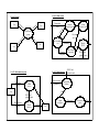
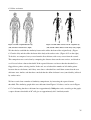
Figure 3.7 The three different types of bounding boxes. From left to right: axis alligned,
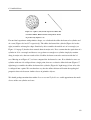
PCA and minimum volume Once the bounding box has been created, we begin generating points inside the box at discrete inter
vals x=y=z. The next step is to determining which of these are also inside the object (polyhed
ron). We do this by casting random rays from the point of interest and determine how many times it
will intersect the boundary (i.e. how many triangles it will intersect). If we have an odd number of
valid intersections then the point is guaranteed to be inside the polyhedron, whereas an even number
will indicate that the point is outside and could therefore be safely discarded. By valid intersection,
we mean that the ray intersects a triangle inside and not at an edge or vertex. A vertex or edge inter
section cannot accurately indicate if the ray passes through or just touches the boundary, and as a
result it is not possible to determine if the point is inside or not. If such an intersection exists, we
cast another random ray.
Determining if we have a valid intersection is quite straightforward and it is an approach based on
the work of Möller and Trumbore [MTT97]. If we define a triangle as a sequence of vertices (V0, V1,
V2) a point P inside the triangle can be defined in terms of its position relative to theses vertices. So:
P=wV0+uV1+vV2 where w,u,v are the barycentric coordinates of P and w+u+v=1. Because w=1
(u+v), frequently just the pair u,v is used. Thus we can determine whether an intersection point is
within a triangle or somewhere else on the plane in which the triangle is lying by inspecting the val
ues of u and v. If 0 ≤ u≤ 1, 0 ≤v≤ 1 and u+v≤ 1 then the intersection is within the triangle. Other
wise, it is in the plane but outside the triangle.
39
3.3 Our improved algorithm
The next part of the algorithm is similar to Betelu's solution, where we select a triangle, define a
plane from the centre of gravity of that triangle and the normal towards the interior of the volume,
and start advancing the plane in a similar fashion. The major difference between our algorithm and
Betelu's algorithm is that every time the plane is advanced we do not need to use marching cubes to
calculate the boundary of the chord set, since we already have triangles. All we need to do is find
which triangles intersect the advancing plane, cut and reconstruct these triangles while keeping the
rest of the object's surface as it was. The boundary triangles below the plane together with the re
constructed triangles below the plane, will form the new boundary of the chordal volume and then
we can go on to calculate the volume in the same fashion as before. The cut and reconstruct idea is
illustrated in Figure 3.8.
Cutting plane ∏
Discarded triangles
n
Reconstructed triangles
Preserved triangles
Figure 3.8 Cut and reconstruct process. Reconstructed triangles (bold) togeth
er with the triangles under the plane form the new object's surface.
40
3.3 Our improved algorithm
1: Reconstruct
2: Keep new
3: Discard
4: Keep
(Plane containment)
5: Keep new
6: Keep
7: Discard
8: Discard
Figure 3.9 The eight possible ways a triangle can intersect with a plane and how it can be reconstruc
ted
This cut and reconstruct strategy, makes using the marching cubes algorithm obsolete, provided of
course we have a pretriangulated surface. If we start with a point cloud, such as typical medical
imaging data, we can use marching cubes or some other triangulation algorithm (e.g. [PWH98])
at the beginning and still use this cut and reconstruct solution to avoid triangulating the surface
every time the surface is advanced. Cutting and reconstructing triangles is very simple. We just find
the intersections between the plane and every triangle, and then depending on the way the plane cuts
the triangle as we can shown in Figure 3.9, we reconstruct accordingly. For complex shapes, for example nonconvex objects, the plane might cut the object into more than
one connected component so it is necessary to determine how many components exist after we cut
and reconstruct the triangles. To do this, we use a simple formula. Initially, all triangles are marked
as unvisited. Starting with an unvisited triangle, the triangle is marked as visited. For each unvisited
triangle adjacent to the initial triangle (the maximum can be three), a traversal is made to that tri
angle and the process is applied recursively. When all adjacent triangles of the initial triangle have
been traversed, a check is made on all triangles to see if they have been visited. If so, the mesh is
said to be connected. If not, the mesh has multiple connected submeshes, each called a connected
component. Each of the remaining components can be found by starting a new recursive traversal
with any unvisited face. We finish our search for connected components when all triangles are
marked as visited.
41
3.3 Our improved algorithm
It is now necessary to see which chordal points are inside which connected component, so a simple
containment check can be used here, similar to that used above, at the beginning of our approach, to
determine the bounding box. However, it is possible that the point xi,, which defines the advancing
plane, might be outside the object or any connected components. This means there is no chord
defined and therefore no volume. So, if we can check whether this is true or not, we can avoid com
puting unnecessary containment of chordal points. We could test xi for containment in exactly the
same way as above, but we have to pay special attention because in this case the boundary of the
chord is going to be an open polyhedron. Therefore a slightly different approach is necessary, which
involves including the plane as a possible lid to the open polyhedron. Before that, an attempt was
made to reconstruct and triangulate the lid of the open polyhedron4. This was successful, regardless
of the increased difficulty5, but the additional computation cost did not counteract any benefits of
this approach. We therefore modified the containment check to deal with open polyhedrons, and
used the boundary integral formula from section 3.2 above, to approximate the volume of the open
polyhedron without any problems. Also, if the random ray will intersect any triangle edge or vertex
as we seen before, we just cast another random ray, instead of trying to determine if the ray crosses
the boundary or just touches it.
The rest of the algorithm is quite similar to that of Betelu et al. [Bet01], and we stop advancing the
plane when vl≥ v0/2 which is the half of the total volume of the object. Another interesting point to
mention, is that Betelu's solution does not include any other criteria for when the cutting plane
should stop. So in theory, the v0/2 criterion might never be met, especially for nonconvex objects
where the plane can exit the object but still vl <v0/2. It is therefore, quite possible that the algorithm
implemented in such a way will keep on iterating forever. See Figure 3.10 for a case when vl will al
ways remain less than v0/2. There are many solutions to this problem, the simplest of which is to check that l∆d does not exceed
4 Note that after cutting and reconstructing the triangles the polyhedron will remain open where the cutting plane was.
5 In 3dimensional computational geometry intersections between points and rays do not really exist. Such intersec
tions are approximated with minimum distances. Trying to triangulate a polygon in such circumstances, is a very
complicated and time consuming process, where the problems of computational geometry described previously in
section 3.1 are fully realised.
42
3.3 Our improved algorithm
the main diagonal of our bounding box, and when it does, we can stop advancing the plane. We call
this method the diagonal distance. The other way, is to cast a ray from the current point xi and inter
sect it with the sides of the bounding box, making sure that the distance of the line segment between
xi and the intersection point has not been exceeded by l∆d. Another way, which is the one we have
implemented, is when xi exits the volume, to cast a ray in the same direction as the normal of xi, and
see if there are any reentry points to the volume. If reentry points are found, we can advance the
plane П directly to the first reentry point. This of course will require us to check for intersections
between the ray and every triangle in the boundary of the object, every time xi exits the volume. If
the object contains many triangles, this might not be the best choice, since intersection checking can
take a long time. An even more efficient way would be to determine the entry and exit points of xi
at the beginning, before we start advancing the plane, so we know that when the number of entries
have been exhausted, xi will never be back in the volume, and thus we could safely stop the itera
tion with that specific triangle and carry on to the next. An illustration of the diagonal distance and
raycasting solutions are provided in Figure 3.11.
This is a very important issue, because it can considerably improve the running time of the al
gorithm and even if the vl≥ v0/2 criterion is met, we can still see substantial improvements, where
the plane can be advanced straight to the next entry point. Table 3.1 shows just how this solution
can affect the running time of the algorithm. Note that the improvement increases are not uniform
from one object to the other, but rather that they depend on the topology of the object (voids inside
the object, how many times xil exits and reenters and so on). So using the raycasting method in
stead of the diagonal distance on a sphere is not expected to bring about any noticeable improve
ment.
Execution time
Method
Body (292 triangles, Δ d=200
Torus (256 triangles, Δ d=200
pixels)
pixels )
Previous algorithm
Infinite loop
Infinite loop
Diagonal distance
6h 37m 2 sec
3 h 18 m 37 sec
47 m
5 m 34 sec
Raycasting
Table 3.1 Different methods for stopping the advancing plane and their impact on execution time6.
6 The program was executed on a dual Celeron 550 Mhz PC with 194MBytes of RAM.
43
3.3 Our improved algorithm
So, after all our emendations the final algorithm is as follows:
1. Read the triangulated data
2. Compute the volume v0 of the object
3. Generate points inside the volume
4. For each triangle Ti in the object do
4.1.Compute its normal ni and centre of mass xi and set iteration variable l
4.2.Define a plane П with normal ni containing xi
4.3.While v<v0/2 do
4.3.1.Increment l
4.3.2.If l∆d >bounding box diagonal break
4.3.3.Advance plane П by ∆d
4.3.4.Cut and reconstruct triangles under the plane
4.3.5.Find connected components
4.3.6.Find in which connected component xil is contained
4.3.6.1.Compute the volume of this connected component
4.3.6.2.Find all the chordal points x' inside the connected component
4.3.6.3.Interpolate to find the volume of the chord when the plane is at x'
4.3.6.4.Set E(x,V)=min(E(x,V), uint((xxi)∙ni)) 4.3.6.5.Store optimal normal n for x'
4.4.End while loop
5. end for loop
6. For every chordal point x'
6.1.Find the divergence of the optimal normal N field
6.2.If divergence > threshold output to skeleton file
7. End
∏0
xi
∏1
v0/2
∏2
xi1
∏3
xi2
∏4
xi3
} undefined
} undefined
} undefined
}undefined
Figure 3.10 The problem of the foreveradvancing plane. This is
when xi is outside and the chordal volumes are undefined
44
3.3 Our improved algorithm
xi
∏0
v0/2
∏1
xi1
∏2
xi2
∏0 entry
xi
Stop here
exit
diagonal
v0/2
Stop here
Figure 3.11 Some solutions to the forever advancing plane problem. Using the diagonal distance (left) and
raycasting to detect entry and exit points (right). It is obvious that from the example sketched, the raycast
ing method is in principle far superior to the diagonal distance.
3.4 SHOCK COMPUTATION
Let us consider a shape represented by a curve C0(s) undergoing a deformation, where s is the para
meter along the curve and let each point of this curve move by some arbitrary amount in some arbit
rary direction, according to Kimia et al. [KTZ95] the evolution of the curve can be described as:
{
C
= s , t n
t
C s , 0 = C 0 s
}
where n is the outward normal, t is the time duration (magnitude) of the deformation and is ar
bitrary. Furthermore, the deformation could be a linear function of curvature =0+1. In this case,
the space of all possible deformations is spanned by two parameters: the ratio of the coefficients
0/1 and time t, which constitute the two axes of the reactiondiffusion space. In this space, a shape
can be described by a set of shocks that develop during the evolution. These are points where some
information is lost during the deformation process, such as discontinuities of the normals of the
shape's boundary or the collision of remote portions of the shape through its interior. The connec
tion between shocks and the skeleton is that the reaction axis corresponds to a grassfire simulation,
45
3.4 Shock computation
and the set of shocks that form along that axis, give us Blum's skeleton. There are also shocks that
form along other axes of the reactiondiffusion space and according to Kimia et al., they can be clas
sified into four types:
1. A firstorder shock is a point of discontinuity in orientation of the boundary of the shape.
Intuitively the shock is formed by a protrusion or corner point in the boundary.
2. A secondorder shock is a point where two distinct nonneighbouring boundary points
joint, but none of their immediate neighbours collapse together. Intuitively, it is formed
just before a splitting of the shape into two parts at a “neck”.
3. A thirdorder shock is a point where two distinct nonneighbouring boundary points join
such that the neighbouring points also collapse together. Intuitively, a collection of third
order shocks can be thought of as a bend.
4. A fourthorder shock is formed when a closed boundary collapses into a single point. In
tuitively, in terms of the evolution a fourthorder shock is a “seed” from which a shape is
born.
Figure 3.12 shows typical examples of all types of shocks.
Although intuitively, the above definitions of shocks cannot be easily used in algorithms for shock
detection, it is possible to use standard techniques such as central differences or gradient operators.
However, these methods will only detect firstorder shocks. As we have seen above, the original al
gorithm used finite differences for shock detection. We used a slightly better method, the Zucker
Hummel operator [ZH81] to detect the gradient and therefore compute the derivatives in the x,y,z
directions.
The ZuckerHummel operator samples all 27 neighbours in a 3x3x3 grid and smooths out the gradi
ents much better than the central differences operator. Furthermore, preliminary tests with our data
have shown it to better approximate the divergence and the behaviour of the thresholding used to
detect skeleton points seem to be more stable than previously, in a variety of data. Results from this
gradient operator are presented in chapter 6, and the definition of the operator can be seen in the ap
46
3.4 Shock computation
pendixes. The ZuckerHummel operator produces results equivalent to those obtained with a 3d So
bel gradient detector, the masks for which can also be found in the appendices.
d
P
d
Firstorder shock
P
Thirdorder shock
P
Secondorder shock
P
Fourthorder shock
Figure 3.12 The four types of shocks created during the deformation process
However, such standard techniques blur across discontinuities, which is where shocks usually lie,
and provide unreliable estimates of geometric quantities, such as orientation. Such quantities are im
portant for shock detection and estimating of shock velocity, which for example may be used to
group shocks. In addition, detection of higher level shocks cannot be carried out by means of such
methods, and also detection of shocks on a discrete grid is a difficult problem. Shocks occur as dis
crete events in time and space. It is very easy to miss them if computations are restricted to grid
points, and not taking advantage of the continuous propagation information that exists in curve
evolution. Finally, distinguishing between singularities that are discretisation artefacts and those
that are weak but structurally valid shock points is also a problem. This is similar to the edge detec
tion dilemma, where we are looking for a distinction between weak edges and false positives. The
solution used there, for example with the Canny edge detector [Ca86], was to carry out the detection
task in two stages. A local detection stage, identifying true as well as some false edges, and a global
interpretation stage, which strengthens edges through a relaxation process. Siddiqi and Kimia [SK96], have proposed a similar method for shock detection, by not only relying
on better (subpixel) shock detection and classification, but also on the creation of a shock grammar
47
3.4 Shock computation
to detect global interactions between them. This shock grammar enables us to rule out impossible
combinations and to group shocks into connected components. This can lead to a hierarchical rep
resentation, functionally related to the object's parts, protrusions and bends. Even more recently, Siddiqi et al. [Sid99] have introduced a new algorithm for divergence based
skeletonisation by simulating the eikonalequation. Their method is based on Hamiltonian physics
that offers a number of computational and conceptual advantages for shock tracking. Although the
resulting skeleton is not affine invariant, they proposed a more efficient and robust algorithm for di
vergence computation and shock detection. Their idea is based on the fact that when shocks are
formed, the conservation of energy principle in the Hamiltonian system will be violated and energy
will be absorbed. This loss of energy can be used to detect shocks. By using the divergence theor
em, it is possible to detect the net outward flux per unit volume (when considering a volume with an
enclosed surface). Where the flux is negative, indicated areas where energy is lost (sink points).
These sink points are also the shock points. However, there is considerable work to be done in this
area especially in the simulation of the eikonalequation in 3d and also on the proposed algorithm
for divergence calculation. We have tried to use their idea instead of using a gradient operator, but
the results where not that satisfactory, as we will examine in later chapters.
48
4 Analysis and design
4 ANALYSIS AND DESIGN
This chapter describes the introductory phases of our software engineering process, in which the re
quirements for the software are established and specified in detail for further development. We start
with a dataflow model, to illustrate how data is processed by the system. We continue with the re
quirements definition, which is an abstract description of the services the software should provide
and the constraints under which it must operate. We conclude with the design of the software, fol
lowed by a brief discussion of why the particular design was chosen over competing methodologies,
and any problems we had to overcome.
4.1 REQUIREMENTS AND SPECIFICATION
4.1.1 DATAFLOW MODELS
What follows is a series of dataflow models, produced as part of the analysis process which help
depict the relationships between the system components and the system and its environment. Fur
thermore, they depict how data flows through a sequence of processing steps, and how it is trans
formed at each step before moving to the next stage. We start with the context diagram, where the
overall skeletonisation system is illustrated together with the data that moves in and out of its
boundaries, to the environment (the user). The triangulated object and the skeletonisation paramet
ers are passed as input, they are processed by the system and the output is the skeleton, with the op
tion of the eroded object as well. If we pay closer attention to the skeletonisation system (level 1) we can see that it is composed of
two main processes, the affine erosion and the shock detection. The skeletonisation process will cal
culate the erosion levelset function (E.L.S.F.) for every chordal point x' and the optimal normals
that produce this E.L.S.F. These data are passed to the next process, which together with parameters
input by the user, are used to detect the shocks and thus the skeleton points. Going down to a final
level of detail (level 2), we can see the subprocesses for affine erosion and shock computation.
These are selfexplanatory, since they follow the logic of the algorithm given in section 3.3.
49
Level 2: Affine erosion
User
User
Tri
ang
u
obj lated et
n
tio
a
s
i
on ers
let met
e
Sk para
leto
Ske
n
Triangulated
object
User
l
na
er ts
t
In oin
p
Skeletonisation
system
E
(o ros
pt io
io n
na
l)
Generate
internal points
lse
a
e/F
ru
Do containment
test
User
T
Triangulated
object
Level 2: Shock detection
User
E.L.S.F. and optimal normals
Skeletonisation
paramaters
Skeletonisation
parameters
Affine
erosion
Shock
detection
E
(o ros
pt ion
im
al)
Skeleton
Reconstructed
object
True/False
Connected
components
Level 1: Skeletonisation system
Cut and
reconstruct object
Find connected
components
c.c
Context diagram
Erode
Calculate E.L.S.F.
E.L.S.F. And
optimal normals
E.L.S.F. And
optimal normals
Approximate
gradient
Gradient
Compute
divergence
User
Divergence
Find skeleton
points
Skeleton
4.1 Requirements and specification
4.1.2 REQUIREMENTS DEFINITION AND SPECIFICATION
Having a basic system model with which to work, we will now examine the requirements of this
system. This is basically a more precise description of the functionality of the system, and under
what constraints it should operate. We will start with the definition of the requirements, which only
depicts the external behaviour of the system and are not concerned with any design characteristics.
We have divided requirements into functional, which are just statements of the system services, and
how the system should react to particular inputs, and to nonfunctional, which are constraints im
posed on the functionality of the system and the development process.
Functional requirements
Read input data from user
The system should have the ability to read and process input parameters from the user and
also read a triangulated polyhedron from an OFF file. It should store the OFF file in com
puter memory in such a way that it can be processed later by other parts of the system.
(1)The user inputs erosion and skeletonisation parameters together with the triangulated ob
ject when running the program.
(2)The system stores the parameters in appropriate variables for later processing.
(3)The OFF file is opened, the data is read and stored so that processing (such as fast se
quential access, copying and so on) is facilitated.
Erosion
The system should use the stored object data and by following the steps that the algorithm
stipulates, it must calculate the E.L.S.F.s for every point inside the object and if the user re
quires it to erode the shape, it must do so.
(1)Access the stored triangulated object data, and carry out what is describe in the algorithm,
in computational geometry, without affecting the original data.
(2)Provide functionality, including to other parts of the system, such as: point containment
testing, volume approximation, connected components detection, shape reconstruction
51
4.1 Requirements and specification
and E.L.S.F. computation for every chordal point.
(3)Store the output of the processing (E.L.S.F. and optimal normals) to a file, or in memory
so that it can be accessed by the skeletonisation subsystem.
(4)If necessary, erode the shape and output the eroded data to a file in an appropriate format
(e.g. 3d vertex data), so that is could be displayed by conventional 3d data viewers such
as [GLD03].
Detect shocks
The system should read the eroded data (E.L.S.F. and optimal normals) and by using an ap
propriate gradient operator or other method detect which points are shock points. This shock
points should then be written to a file.
(1)Read the optimal normals and use a 3d gradient operator to approximate the divergence.
(2)Detect the shock points by using a simple threshold.
(3)Write these shock points to a file, in a conventional format.
Nonfunctional requirements
Usability: Based on projects of similar size and functionality we have concluded that since the sys
tem requires no user interaction and supervision, apart from the initial data and parameter input,
users should be able to use all the system functions with minimal training. Portability:The system should be implemented in a language where it would be possible to compile
it for different platforms. The obvious choice would be STD C++, and if possible ISO C++.
Reliability: Based on current systems and user requirements, the system must have a mean time to
failure of 4 weeks of continuous execution, considering that most 3d objects with medium to high
level of detail, will take >1 week to compute.
Delivery: The software must be completed on schedule and all the necessary testing and documenta
tion must be carried out. On schedule here means by the submission deadline of the CVIPGS MRes
52
4.1 Requirements and specification
project dissertations.
Robustness: There must be zero probability that the of the original data might be corrupted, and low
probability of corruption of the produced data, after failure.
Speed: The design and implementation of the system (together with choice of language) should not
considerably increase the estimated execution time of the algorithm.
4.2 SOFTWARE DESIGN
At the beginning of the design process, we chose a procedural design for our software, similar to the
one suggested by Betelu [Bet01]. However, it was obvious in that stage, that many parts of the sys
tem required input and functionality from other parts, and this proved to be quite complicated for a
procedural design to handle. Furthermore, as the scale of the design increased, and many portions of
the system were constantly reused, we soon realised that perhaps it would have been better to use an
objectoriented (OO) methodology to capture this complexity, the communication needs and code
reuse requirements. In addition to that, this project is largely based on computational geometry,
which itself is built from simple components such as points, lines, angles, and so on, which are
combined in order to build a more complex structure. OO design can capture this behaviour easily
because of its special characteristics, such as inheritance, aggregation, data abstraction and so on.
4.2.1 OBJECT ORIENTED DESIGN
So, what follows is a a class diagram (Figure 4.1), which contains the set of classes, and their rela
tionships. This diagram aims to capture the static design view of the system. What is interesting to
note from this diagram, is that akin to the bottomup way that computational geometry is built, so is
our system. We can see the Vertex3D class as being the building block of our system, and from that,
almost all other classes emanate. Another thing to note, is the Polyhedron class, which has most of
53
4.2 Software design
the functionality of our system, and therefore the most attributes, methods and importance. A poly
hedral object and the operation on it, was the main focus of our algorithm, and therefore most of the
implementation time and effort was based around the methods of this class. Test for
Test for
Test for
1
Generate
3..*
1
1,2
1
2
has inside
3
1..*
Contains
1..*
Figure 4.1 Class diagram of the skeletonisation system
54
4.2 Software design
The next figure (4.2), is an object collaboration diagram, which shows the organisation of the ob
jects that participate in an interaction, in an attempt to capture the dynamic view of the system. We
have only modelled the calculation of the E.L.S.F. since that is the most important and complex op
eration. We can see the messages between the objects been passed in the appropriate sequence, to
generate one iteration of our algorithm (i.e. one advancement of the cutting plane). As we can see
here, the polyhedron object is the main object in computing the erosion, and most of the processing
is done by function calls instantiated by the object itself. As we can see from the two diagrams,
most of the other objects are not directly associated with the actual execution of the algorithm, but
through the attributes and methods of the polyhedron and cutting plane. It would be equally valid, instead of using a bottomup approach and starting from the vertices and
triangles, to use a topdown methodology and create only a few highlevel classes (such as the poly
hedron) and include the vertices, triangles and so on, as attributes. Although this idea would work, it
would resemble a procedural design, and so defeat the point of using an objectoriented methodo
logy in the first place. Scaling a system of that procedural type would be quite difficult, especially if
we discover during the implementation that using a polyhedron is not practical. Using a building
block idea like that describe above, enables us to add and remove classes from our system as neces
sary and to make alterations without affecting other classes. Furthermore, it is easier to port the sys
tem, as a collection of libraries, to another platform, to insert new libraries (such as polygons, tetra
hedra etc) that follow this bottomup approach or even to be used as new building components in
another system that uses computational geometry. 55
5 Implementation and testing
5 datafile:OFFfile
1 generatePoly()
4 cutNReconstruct()
cuttingPlane:Plane3D
3 advance()
poly1:Polyhedron
2 volume()
5 getConnected()
6 pointInPolyhedron() Figure 4.2 Object collaboration diagram for compute ELSF functionality
IMPLEMENTATION AND TESTING
This chapter presents some of the most important issues and difficulties we had to face during the
implementation process, and what steps we took to overcome them. We go on to discuss the details
of the algorithm complexity and attempt to approximate it using a qualitative approach. We con
clude with the testing results, which aim to expose errors in the implementation and determine the
capabilities of the system.
5.1 IMPLEMENTATION ISSUES
Our implementation follows the initial design quite closely, with only a few minor modifications
made, such as a few additional attributes in some classes, like boolean flags and so on. We origin
ally implemented a linkedlist template that we could use with different types of variables and store
different data, such as vertices, boundary data and so on. Because most of message and parameter
passing between objects is done via pointers, our linkedlist template proved to be very unstable un
der such circumstances and caused random segmentation faults. Furthermore, because of the fact
that it allocated memory for variable storage, but did not deallocate it appropriately, it generated
severe memory leaks. If we consider that the program executes over a long period of time, this
would cause serious problems and even cause the operating system to halt. 56
5.1 Implementation issues
We therefore decided to overhaul the whole system and use the C++ standard template library
(STL) and most specifically the vector class. This is a linkedlist template similar to ours but
without the serious memory leak problems. There are still a few minor memory leak, but there are
so small that they do not pose any immediate threat to the execution of the program, even if it is has
been running for a considerable amount of time (Table 5.1). In the first three rows we can see the
average number of bytes allocated in every main iteration (approx. 1.8Mb) which are stabilised
from iteration to iteration, and the growth is insignificant. This growth, can be seen in the identified
memory leak, which is 4Kbytes x 2 of nonreoccurring memory loss. This happens once the bound
ing box is created, and a 24byte x 2 reoccurring once in every major iteration. For a modern work
station with hundreds of Mbytes of memory, a 48byte leak is really not a problem. We could easily
fix this problem, but considering Pareto's law its probably not worth the actual effort.
For some parts of our implementation, we had to use the theory and algorithms from [SE03] that we
adjusted and added to our existing system. Particularly, we used libraries for intersections, connec
ted components detection and some definitions of primitives in computational geometry. The fact
that we had designed our system using OO methodology, proved a good strategy when using other
open source libraries.
Number of allocations (approx.)
802
Bytes/Allocation (approx.)
2225.61
Total Bytes (approx.)
1784940
Memory leaks
24 bytes (reoccurring at every main iteration)
double maximum(double array[], int); from extraMath.h
4 Kbytes (once at the creation of the bounding box) double maximum(double array[], int); from extraMath.h
24 bytes (reoccurring at every main iteration)
double minimum(double array[], int); from extraMath.h
4 Kbytes (once at the creation of the bounding box)
double minimum(double array[], int); from extraMath.h
Table 5.1 Table showing the average number of bytes allocated and the memory leaks
One thing we mentioned before is the fact that computational geometry is quite different from ana
lytic geometry. This has been particularly realised here, in the implementation stage, where because
of small approximation errors, arithmetic operations produce unexpected results. Such occurrences
where in the detection of connected components. This is carried out by comparing the sides of tri
57
5.1 Implementation issues
angles to see if they match and therefore form a mesh. At the beginning, when the object was com
plete, there is no problem with such comparisons, but when we cut and reconstruct the object, the
new triangles might not fall exactly next to each other. This leads to detection of more connected
components than normal. We therefore had to manually examine every vertex of every triangle of
every identified connected component, to check for any degeneracies or triangles that were almost
connected. From carrying out all this laborious checks, we managed to extract an appropriate
threshold to counteract these computational geometry problems.
Similar such thresholds were introduced throughout different functions of the software, such as in
tersections and vertex comparisons, and as a result (because of the buildingblock approach of con
structing our geometry) they are interdependent. What this means is that changing one threshold
might cause another to fail, and by causing a chainreaction effect, cause the system to produce the
wrong results. We therefore had to find a balance between them, based on trial and error. We exper
imented with data, where we knew the results already, and adjusted the thresholds to get the expec
ted output.
5.1.1 ALGORITHM COMPLEXITY
In this section we will present an estimation of the algorithm complexity as a way to characterise its
efficiency. We have estimated the efficiency as the function f(n) representing the maximum number
of primitive operations required for an input of size n, and given in bigO notation. The approach
we used for this estimation, was to consider the fundamental components of the system, approxim
ate their individual complexities and then work upwards to get the overall algorithm complexity.
Our methodology for complexity estimation is based around a qualitative approach proposed by
[Che03], which has shown to lead to the final asymptotic complexity as the traditional formal ana
lysis techniques do.
We considered the system as two distinct components, the affine erosion and the shocks detection.
Estimating the complexity for the shocks detection was quite straightforward. It is O(N3), since we
have to traverse the whole volumetric array and loop three times to access every chordal point.
58
5.1 Implementation issues
However, since we already have the chordal points stored in lexicographic order, it is quite easy to
convert to O(N) by using one iteration, but considering that even with O(N3) the skeletonisation pro
cess takes only a few seconds to complete, it was decided to keep the current solution.
The next part, the affine erosion, was the most difficult part of the system to estimate. We have
identified the following processes as being the most significant for affecting the overall complexity.
Their respective complexities are also shown:
•
bBox(): generate a bounding box to enclose the volume. Complexity= O(N) where N is
the number of triangles in the original object.
•
pointInPolyhedron(): test a single point if it is inside a general polyhedron. Complexity=
O(N) where N is the number of triangles in the original object.
•
generatePoints(): traverse the bounding box and generate points inside it at specific inter
vals t in all directions. While the points are being generated we use the point in poly
hedron method to test for containment. Complexity= O(KJLN) where
K=
Xbounds
Ybounds
Zbounds
and N is the number of triangles in the
, J=
, L=
t
t
t
original object. In the case that Xbounds=Ybounds=Zbounds (bounding cube) then the
complexity becomes O(M3N). Note that this complexity contains the complexities of the
two previous operations (bBox() and pointInPolyhedron()) and although necessary for the
erosion, it can be implemented as a standalone program. It is even possible not include
this function in our system all and read the precomputed internal points from a file.
Therefore, we will include this complexity as a separate entity, when we calculate the
total complexity at the end.
•
CutNReconstruct(): cut the boundary by a plane and reconstruct only those that the plane
intersects. Complexity= O(N) where N is the number of triangles in the original object.
•
FindAdjacent(): find the adjacent triangles of a given triangle in a boundary.
Complexity= O(N) where N is the number of triangles in the original object.
59
5.1 Implementation issues
•
FlagConnected(): recursive function that looks if a triangle has adjacent triangles, and if
so sets their connected flag to true. Complexity= O(N) where N is the number of triangles
in the original object.
•
GetConnected(): find the connected components in a given polyhedron.. Complexity =
O(N2) where N is the number of triangles in the original object. Note that this function
makes use of FlagConnected() and FindAdjacent() and so it includes their respective
complexities.
•
pointInOpenPolyhedron(): similar function to pointInPolyhedron() that tests a single
point for being inside a general, open polyhedron. Complexity= O(N) where N is the
number of triangles in the original object.
Any operations such as assignment, comparison, multiplication, addition and so on, and any se
quential combination of those where no iteration is involved (e.g. an intersection between a line and
a triangle), have been estimated as having constant complexities of O(1) and therefore have been
merged with linear, quadratic and cubic complexities, since O(1)⊂O(N)⊂O(N2) and so on.
Going back to the main function and considering all the above calculated complexities the final
complexity will be:
[ [
O M 3 N O N O L
generatePoints
ON
main loop while loop CutNReconstruct
O N 2
GetConnected
O K
for loop
where N is the number of triangles in the object, L=
ON
pointInOpenPolyhedron
O R O N O S
for loop
for loop
for loop
Xbounds t 2 Ybounds t 2 Zbounds t 2
d
]]
,
t is the volume discretisation size, d is the distance we advance the plane in every iteration, K is
the number of connected components, R is the number of chordal points x' inside the volume and S
the number of reentry points identified by our intersection test.
By doing the calculations and merging complexities we get:
O M 3 N O N 3 LO L N 2 RK O NLS
Remember the first term O(M3N) is the complexity of the generatePoints() function and we do not
wish to merge this as we mentioned before. Now, considering that 2<S<<N because the reentry
points will never be as many as the number of triangles for a closed volume, we can say that N3L >
60
5.1 Implementation issues
NLS and merge the complexities. Furthermore, the number of connected components are usually
between 1 and 10 and so much less than N, therefore 1<K<<N and we can simplify O(LN2RK) to
O(LN2R) since we are not going to considerably affect its asymptotic behaviour. So we end up with
O M 3 N O N 3 LO L N 2 R . From here, we can safely assume that the number of chordal
points for a normal execution of the program will be R>>N and so N3< N2R. This means that
O(N3L) can be merged with O(LN2R). Taking this into account and introducing the shocks detection complexity we have:
1. generate internal points complexity: O(M3N)
2. affine erosion: O(LN2R) which is approximately > O(N4)
3. shocks detection: O(N)
These estimations are dependent on the following parameters. The number of triangles N in the ori
ginal object, the number of chordal points R that we have generated (based on the dimensions of the
object and the t discretisation parameter), the number of times L the cutting plane has to be ad
vanced (based on object dimensions and d ). So, to summarise, the two parameters the user inputs
(t and d) together with the triangles of the object and its volume (dimensions) are what affect the
complexity of the algorithm, which makes sense if we see how changing this values affect the exe
cution time. It would be possible to further simplify these estimates, if instead of using t as a para
meter and calculating the internal points from t and the dimensions of the object, we could pass
the number of desired points as a parameter to the program. This would make the M and R paramet
ers (above) obsolete, but unfortunately would require a redesign of some parts of the system.
5.2 STRESS TESTING
This testing strategy, relies on stressing the system by going beyond its specified limits and determ
ining how well it can cope with overload situations. Normally, we have an estimation of the capab
ilities of the system at design time and we use stress testing to verify them. However in this case,
because of the type of design and inherent complexity, it has proved difficult to make an accurate
estimation of the capabilities of the system. We therefore, decided to use stress testing as a means of
61
5.2 Stress testing
exploring these capabilities and not so much to verify them.
Since we can only test the system as a whole, we have no choice but to make test cases by using the
input parameters. These are the number of triangles in the object, the bounding box discretisation
size t, the distance d that the cutting plane advances, and the dimensions of the object. We have
been experimenting with very high or very low values of these parameters and managed to find
some operational limits of our implementation. These are:
•
Number of triangles: Having tested a variety of input objects with increasing triangle
size, we can conclude that the implementation copes well with datasets of up to 21500 tri
angles. It will fail however, with data sets of 24000+ triangles and cease execution at the
input file reading stage. This indicates that it probably exceeds the allowed memory size
for storing a linkedlist so a new approach is necessary that will store the data in other
parts of memory or in the hard disk and access only portions of it at a time, instead of try
ing to read the whole chunk in one go. As far as minimum triangles are concerned, it can
successfully cope with a tetrahedron (N=4) and even execute for (N=3), which is not a
closed volume and the results will not be geometrically correct.
•
Dimensions of the object:When the dimensions are very small from minX= minY=
minZ= 0, to maxX=maxY=maxZ=0.8 then in order to get the program to work we haver
to set t below 1. In that case the program appears to be working, but does not generate
the internal points correctly. Although it calculates correctly the number of points it
should create, it does actually not create them. This is because traversal in the volumetric
array uses integer arithmetic (discretised) and cannot work when the dimensions and t
are less than 1. As for very large dimensions, we experimented with a variety of different
values and we have seen that for sufficiently large numbers (>8∙107) it affects the volume
calculation, by generating negative numbers for volume approximations. This is a quite
strange behaviour, the exact cause of which we cannot establish at the moment, but it may
be related with the capacity of floattype variables being exceeded.
62
5.2 Stress testing
•
t: We have tested the discretisation size with a variety of very high and very low values
to determine how it can affect the system. Most notably, for extreme values, such as
t=±1025 the program still executes successfully but has no practical meaning since the
number of generated points will be zero (unless of course the object has dimensions in the
order of 1025). At even more extreme values (order of 1050) we noticed the system was not
iterating properly because the dimensions of the bounding box became undefined. This is
most probably associated with the the storage capacity of a double precision floating
point variable being exceeded. For t=0 the program goes into a never ending loop.
•
d: Finally, we tested the distance the plane advanced at every iteration. The results
seemed quite promising, since for very high values (negative and positive are the same,
the only thing that changes is the direction in which the plane travels (upwards or down
wards). For d=0, the the program worked normally, although without any practical
meaning since the plane was outside of the object, did not move and there were no
chordal volumes defined.
So now we can say that we have a better understanding of what the operational limits of our soft
ware are. It would be quite possible at this stage to either adjust the program so that when in a stress
situation like above, to degrade gracefully instead of just crashing and perhaps corrupting the data.
An alternative would be to make the user aware of these operational limits, and ensure the input
data and passed parameters, are within the limits we have identified.
The detailed tests for each of the above cases can be found at the appendices.
63
6 Experiments and results
6 EXPERIMENTS AND RESULTS
This chapter contains a summary of the different experiments we run with our skeletonisation soft
ware, both on artificial and real 3d data (human body scans). Details of such experiments, such as
the parameters chosen and the execution time, together with their results are also presented. These
results are compared with other skeletonisation methods, such as the 3d medial axis and the 3d af
fine skeleton approximation by Jeong and Buxton [JB01] We go on to discuss whether or not the
skeletons produced by our software are indeed affine invariant and noise resistant. We conclude this
chapter with a discussion on the limitations of our algorithm.
6.1 ARTIFICIAL DATA
We chose to experiment with artificial data obtained by Joao Oliveira [OJ03] or generated in freely
available software [W3D03]. This data was a variety of triangulated primitive objects with manifold
meshes in OFF format. We used such data primarily for its simplicity while we were developing
and testing the software, but also to determine how the affine skeleton can compare with the medial
axis, since the medial axis has already being studied in primitive 3d shapes.
Our first example, which can be seen on the left of Figure 6.1 is a triangulated torus with 256 tri
angles. Our skeletonisation program produces the affine skeleton (second image from the left). As
we can see its a 2d flat surface, which is similar to the results of the medial axis transform on a 3d
object. That is, the medial axis of a 3d object will be a surface, apart from rare cases where degen
eracies are produced. Nevertheless, it is interesting to see the results of popular 3d medial axis ap
proximation software, such as [ACK01] and [DG03], that we mentioned in chapter 2 above. The
second picture from the right is the result from TightCocone and the rightmost picture is the result
of medial axis approximation with Powercrust. Although Powercrust cannot produce a connected
skeleton in this case, we can clearly see that both software try to produce a 1dimensional skeleton.
We would like to emphasise the fact that these software do not follow the theory for calculation of
the 3d medial axis but only provide an approximation of it. What this means is that there is a possib
ility that the approximated medial axis is 1dimensional, unlike the affine skeleton that is always a
64
6.1 Artificial data
surface in 2 dimensions. It might be desirable in certain application areas, such as animation and ob
ject matching, to have 1dimensional skeletons, but from a theoretical point of view, the skeletons
produced by Powercrust and TightCocone are not very interesting.
Figure 6.1 (Left) A triangulated torus, (second from left) its affine skeleton, (second from right) medial
axis approximated by TightCocone and (right) medial axis approximated by PowerCrust.
Our next example, takes the same torus and performs a local deformation such that, it reduces the
width of one side of the torus (Figure 6.2 leftmost image). We apply the same algorithm to get the
affine skeleton (second from the left). We can see now that the affine skeleton becomes disconnec
ted. This is not surprising because we know that the affine erosion erodes the object in a uniform
way, removing all the chordal points with erosion levelset function E(x,V) bellow a certain
threshold. It is therefore expected that points in thin parts of the deformed torus may be completely
removed since all the points inside these areas will have E(x,V)<threshold. The skeleton will reflect
this behaviour with discontinuities. We can also see the results of TightCocone and Powercrust
(second from the right and rightmost images respectively) when trying to approximate the medial
axis. Powercrust still produces large discontinuities in the boundary of the medial axis, unlike the
TightCocone that produces a closed skeleton. What is interesting to note here, is that the deformation of the torus, produced some surfaces in the
medial axes approximations by Powercrust and TightCocone. What is even more striking is that
these surfaces appear in places where before there used to be a 1dimensional centreline (Figure 6.1
two rightmost images), even though the thickness of the torus remains the same in both cases. We
can assume therefore, that by locally deforming a shape, we might affect the medial axis in other
areas, not affected by this deformation. This strange property is not exhibited by the the affine skel
65
6.1 Artificial data
eton, which is a 2d surface throughout.
Figure 6.2 (Left) A torus with a local deformation at one side, (second from left) its affine skeleton,
(second from right) medial axis approximated by TightCocone and (right) medial axis approximated by
PowerCrust.
Our next result is from an experiment on a ellipsoid object. In their work, Betelu et al. [Bet00], have
shown that the affine skeleton of en ellipse (the 2d equivalent of an ellipsoid) is a line, whose length
depends on the length of the major axis of the ellipse. An ellipse can also be thought of as a circle
that has been elongated by affine transformation. By virtue of the affine invariance property of the
affine skeleton, the skeleton of the circle (its centre) will be elongated via the same transformation,
giving a line in the centre of the ellipse . This idea can be seen in Figure 6.3. Now that we know that
the skeleton of an ellipse is a 1dimensional line, we can expected that the affine skeleton of an el
lipsoid in 3d, will be a rectangular surface, since this is the equivalent of a line in 3 dimensions.
Figure 6.3 The affine skeleton of a circle an that of an ellipse As we can see in Figure 6.4, this happens to be the case, and the affine skeleton of an ellipsoid is a
2d rectangle (middle picture). The dimensions of this rectangle are dependent on the dimensions of
the axes of the ellipsoid. We also tried to calculate the medial axis of the ellipsoid with Powercrust
and TightCocone. Powercrust did not produce any results, unlike TightCocone, which produced a
2d planar surface (right picture) similar to but not as well defined as the affine skeleton. There
66
6.1 Artificial data
seem to be more jugged edges in the medial axis approximation, probably related with either surface
noise or the low resolution of the ellipsoid. In this case, the medial axis as approximated by Tight
Cocone is a surface suggesting that there is no consistency between the dimensions of skeletons of
different 3d objects. The affine skeleton on the other hand seems to be more consistent and always
produce a 2d surface. This of course is not a proven fact but our opinion which is based on our res
ults.
Figure 6.4 On the left a triangulated ellipsoid and its affine skeleton (middle). On the
right we see an approximation of its medial axis by the TightCocone software.
Now we examine a case where our skeletonisation algorithm will produce a degenerate surface.
This is the special case of the sphere. We know that the affine skeleton of a circle in 2d is its centre
(Figure 6.3), similar to the 2d medial axis of a circle which is its centre by definition. In 3d dimen
sions, the affine skeleton of the sphere, is a cluster of points approximately in the centre of the
sphere (Figure 6.5 middle image). This is because the erosion of a sphere will always be a sphere
with a diminishing radius. As the sphere erodes, this cluster of points will always be equidistant
from every point in the boundary (by distance here we mean the volume of the chordal set as
defined in chapter 3) and therefore they will be points in the affine skeleton. In terms of shocks,
these can be though of as fourthorder shock points, which are generated when a closed boundary
collapses under erosion into a single point. We have a cluster instead of a single point, due to the
difficulty identifying such higherorder shocks in computational geometry, as we have mentioned in
chapter 3 previously. When we tried to approximate the medial axis as before, we got this strange
linear skeleton from TightCocone (Figure 6.5 right image), while Powercrust could not approxim
ate the medial axis of our sphere at all. We have to admit that we could not explain why these very
popular medial axis approximation software produced these results.
67
6.1 Artificial data
Figure 6.5 A sphere (left) and its degenerate affine skel
eton in the middle. On the left the strange linear skelet
on produced by TightCocone.
For our final experiment with primitive shapes, we calculated the affine skeletons of a cylinder and
of a cone (Figures 6.6 and 6.7 respectively). The affine skeleton of the cylinder (Figure 6.6 on the
right) resembles an hourglass shape. Intuitively, this resembles the medial axis of a rectangle (see
Figure 1.1 in page 5) that has been rotated about its major axis. If we assume that the equivalent of a
cylinder in 2d is a rectangle and that we can go from a rectangle to a cylinder simply by rotation
along its major axis, then our results of the 3d affine skeleton seem to be consistent with the 2d
case. Moving on to Figure 6.7, we have computed the skeleton of a cone. If we think of a cone as a
cylinder with one side collapsed into a single point, then we see that its affine skeleton (Figure 6.7
right image) resembles the affine skeleton of the cylinder (Figure 6.6 right image) if one of its side
is collapsed into a point. We can therefore say, that the affine skeleton will retain the topological
properties that exist between similar classes of primitive objects. We should perhaps mention that neither Powercrust nor TightCocone could approximate the medi
al axes of the our cylinder and cone.
68
6.1 Artificial data
Figure 6.6 A cylinder (left) and its affine skeleton (right)
Figure 6.7 A cone and its affine skeleton (right)
6.2 REAL DATA
We will now apply our skeletonisation algorithm to real data, captured by the Body Lines scanner
[Hor95] available at the computing department in UCL. These are triangulated 3d scans of human
bodies at different resolutions (i.e. number of triangles). A small sample can be seen in Figure 6.8.
Figure 6.8 Human bodies in different resolutions. From
left to right: with 292, 500, 1000 and 5000 triangles re
spectively
The first results of applying the 3d affine skeleton to human body scans can be seen in Figure 6.10.
This is the skeleton from a low resolution triangulated body with 292 triangles. The first results are
far from perfect, but seem quite promising. We can see a front view of the skeleton (Figure 6.10 left
image) and a side view (Figure 6.10 right image) that clearly illustrates that the skeleton is 2dimen
sional, consistent with the results we produced in the previous section. The biggest visible problem
69
6.2 Real data
with this skeleton is that it contains numerous discontinuities.
We believe that these discontinuities are caused by both a practical and theoretical problems. The
theoretical of course is the computation of shocks as we have mentioned many time throughout this
report. The practical problem is the parameters with which the program is running. As we have seen
is section 5.1.1 the complexity of the algorithm depends on the three parameters. The number of tri
angles N in the body, the volumetric array discretisation size t and the distance d the plane
travels with every iteration. The higher the number of triangles and lower t and d are, the longer
the program will take to execute. To produce the results in Figure 6.10 we had to use a model with a
relatively low number of triangles (292) and high number for t and d (200 pixels and 200 pixels
Figure 6.9 The affine skeleton
respectively). We did this to save computation time, because as we will see later the skeletonisation
process can take a very long time to finish.
of a 500 triangle human body.
The drawback of using low resolution objects with such high values for t and d, is that the ap
proximation of chordal volumes via linear interpolation (see section 3.2.1) will be very crude, and
so will be the computation of the skeleton. In addition, because an object with a high number of tri
angles approximates volume much better than an object with a few triangles, volume computations
(which are fundamental processes in 3d affine erosion) will be much more accurate when N is large.
Finally, the more triangles, the more cutting planes will be generated at different orientations. This
means that we will sample the chordal points closer to the theoretically large number of orientations
necessary to compute the erosion levelset function E(x,V).
To prove this, we have executed the program with a 500 triangle model and t=d=200 pixels, and
calculated its affine skeleton. The results can be seen in Figure 6.9. Not that a 500 triangle model
can be defined as high resolution, but still the improvement from the skeleton in Figure 6.10 is sig
nificant. Straight away, we see that the connectivity of the skeleton points has been improved, espe
cially in the torso, head and shoulders area. This slight increase in resolution brought about a sub
stantial increase in execution time. Whereas the first the 292 triangle model in Figure 6.10 took ap
proximately 35 min 41 sec to execute, the 500 triangle model in Figure 6.9 took in excess of 1 hour
and 45min to complete. This is more than a threefold increase in execution time for a 2.5 increase in
70
6.2 Real data
surface triangles. The gap between resolution increase and execution time increases as we increase
the number of triangles N. We will see more details of this later on.
6.2.1 TRIANGULATION
We should mention here once again that the output of our algorithm is a point cloud (i.e. disconnec
ted points in 3d space). The medial axis approximation software that we have seen above (Power
crust and TightCocone) produce a triangulated surface by computing the convex hull of the object.
This might produce acceptable results for convex objects, but for complex nonconvex objects such
as human body scans the triangulated surface is not very accurate. We have used a different tech
nique (although not implemented as a requirement of this project) called the 3d shape [EM94].
Alpha shapes can be thought of as generalizations of the convex hull of a point set, where by vary
ing a parameter (called alpha), we can get shapes ranging from crude to fine. The most crude shape
is the convex hull itself, which can be obtained when alpha is very large. As alpha decreases, the
shape shrinks and develops cavities that may join to form tunnels and voids. These cavities are what
we are interested in, because they are very common in complex objects such as human models (e.g.
cavities under the arms and between the legs). The results of shape triangulation in the skeleton
from Figure 6.10 can be seen in Figure 6.11. The skeleton which now is a triangulated surface,
looks more complete, with fewer discontinuities.
The problem with the shape approach, is that because it depends on the right choice of the alpha
parameter, and this parameter is difficult to find, most of the times constructing the triangulation of
the boundary of a shape requires trial and error. An alternative to shape is the marching cubes
[LC87] but will not work sufficiently if there are many disconnected points or boundary noise.
71
6.2 Real data
Figure 6.10 Affine skeleton of a
292 triangle human body. (left)
Figure 6.11 The same skeleton
that has been triangulated .
front and (right) side view.
6.2.2 MEAN CURVATURE THRESHOLD
As we have already mentioned, in order to find the shock points in E(x,V)=constant we need to se
lect those points where the mean curvature is greater than a fixed threshold . Betelu et al. [Bet01]
have proposed that this threshold is in the order of the inverse of the discretisation size of the volu
metric array (see section 3.2.2). We have tried this approach and found it to be appropriate when we
used the intermediate difference operator to compute the divergence ∇.n(x) of the optimal chord
normals. However, when using the ZuckerHummel gradient operator, the same threshold does not
apply. We therefore used trial and error to find another that produced a good approximation of the
3d affine skeleton. Figure 6.12 shows how the approximated skeleton is affected by different
choices for . After trying a variety of thresholds, we came to the conclusion that for =7 we get
the most eyepleasing results. We are not sure what the significance of this number is, and how it is
related with the choices of parameters t and d, but we found it to be consistent among all experi
ments we carried out with real and artificial data (see section 6.1), and always produced the best res
ults. 72
6.2 Real data
Figure 6.12 The affine skeleton of a 292 tri
angle body, for different thresholds (from
left to right) =9, =7, =6
6.2.3 COMPARISON WITH OTHER METHODS We have also computed an approximation of the medial axis skeleton by using the TightCocone
and Powercrust programs, in order to compare them with our affine skeletons. Initially we used the
same 292 triangles body model (Figure 6.8 leftmost image). Surprisingly, TightCocone could not
produce any results whatsoever, whereas Powercrust produced the leftmost skeleton in Figure 6.13.
Compared with our results in Figure 6.11, it is straightforward to see that our algorithm performs
much better with lower resolution models, producing a skeleton that still resembles the topology of
the human body. When we used a higher resolution model with 500 triangles (Figure 6.8 second
image from the left) both the Powercrust and TightCocone produced much better results with very
good connectivity (Figure 6.13 middle and right images respectively). When compared with the af
fine skeleton of the same 500 triangle body in Figure 6.9 it is clear that the skeletons from Power
crust and TightCocone perform much better as the number of triangles increases. Note however, that the skeletons in Figure 6.13 are triangulated whereas ours is not, and further
more, Powercrust and TightCocone are specifically built and adjusted to produce eyepleasing me
dial axis skeletons. These skeletons are subjected to a variety of enhancing procedures (such as
noise removal) and do not necessarily follow the extension of Blum's [Blu64] medial axis theory in
3d (i.e. using maximal spheres to detect skeleton points). This becomes more apparent if we do a
73
6.2 Real data
comparison between the Powercrust and TightCocone skeletons. Even though they should repres
ent the same skeletonisation method and in theory should look similar, they do not. Note the signi
ficant differences between the hip and head regions in the middle and right skeletons of Figure
6.13. Finally, we would like to make a visual comparison of our affine invariant skeleton, with the one
by M.S.Jeong and B.Buxton [JB01]. Their method is based on computing the 2d affine invariant
skeletons of horizontal slices of the human body and bringing them together to form an approxima
tion of the 3d affine invariant skeleton. Such a skeleton can be seen in Figure 6.14. This skeleton
has been produced form a high resolution human body scan, much more detailed than our example
in Figure 6.8, in and so it exhibits very good connectivity. The 3d skeleton that is produced by
means of 2d skeletonisation, has different geometrical properties from our 3d affine skeleton. If we
look at the left skeleton picture in Figure 6.14, we can see that the skeleton parts of the head, arms
and legs have approximately the same thickness. This clearly does not correspond to the original
human body model, where the head is much ticker than the limbs. Our skeletonisation method pro
duces a skeleton (Figure 6.11) with areas of variable thickness that correspond to the parts where
the original body is thick respectively.
In addition, note that the arms and (if we examine very closely) the legs are disconnected from the
body. This is because of the limitation of their method, which can only deal with one connected
component at a time. Cutting a horizontal slice at the torso will produce three connected compon
ents, which will be the closed curves formed by the intersection of the object's vertices and the cut
ting plane, and will correspond to the two arms and the torso. The 2d affine invariant skeleton can
not cope with more than one curves at a time, and so, applying such a method in a 3d nonconvex
objects will require the segmentation of the object into separate connected components (for a human
body, the torso with the head, and the limbs). This segmentation process is not easy or unique, since
a human body can be captured in many different orientations and positions, and will require manual
intervention. In that sense, our algorithm is superior to that proposed by M.S.Jeong and B.Buxton
[JB01], since it can cope with any amount of connected components without the need for manual in
tervention, provided of course we are applying the algorithm at one object at a time.
74
6.2 Real data
Figure 6.13 The medial axis of a 292 triangle model produced by
Powercrust (left), the medial axis of a 500 triangle model by Power
crust(middle) and the medial axis from the same model by Tight
Figure 6.14 3d affine skeleton approx
imation by 2d crosssectional slices
Cocone (right).
6.3 NOISE RESISTANCE
We will now see how robust the 3d affine skeleton is when noise is added to the boundary of the
original object. We started by adding noise to a triangulated human model by randomly moving the
surface vertices (i.e. multiplication of every vertex with a random value) and got the resulting noisy
body in Figure 6.15 on the right. The noise values where chosen from a normal distribution with
mean zero, variance one and standard deviation one.
75
6.3 Noise resistance
Figure 6.15 The original human body
Figure 6.16 The affine skeleton of the original body
(left) and after random noise (right)
(left) and the affine skeleton of the noisy body (right)
We then had to establish the similarity between the affine skeleton of the original body ( Figure
6.15 on the left) and the affine skeleton of the body with surface noise (Figure 6.15 on the right).
To do this, we compared every vertex from the first skeleton, with every vertex from the second.
This comparison was carried out by computing the distance between the two vertices, and check to
see if it was below a chosen threshold. If the squared distance was lower than the threshold, we
flagged these points as being similar. In the end, we calculated the number of all similar points
between the two skeletons, and if they were above a threshold we could then assume that the two
skeletons were similar, and therefore conclude that the affine skeleton is not (considerably) affected
by surface noise.
We have carried out a number of similarity comparisons, by increasing the square distance
threshold. The similarity graph of the two skeletons from Figure 6.16 above, can be seen in Figure
6.17. Considering that these skeletons have approximately 5000 points each, according to the graph,
a square distance threshold of 108 will give us approximately 94% similarity match. 76
6.3 Noise resistance
Figure 6.17 Graph plot of the number of similar
Figure 6.18 The similarity graph plot for the original
points between the two affine skeletons, in relation
and noisy skeletons, as computed by Powercrust.
to the square distance threshold.
However, we are not quite sure what would constitute an appropriate threshold. One way that we
could devise a threshold, would be to consider the volumetric array discretisation size t. We have
computed these skeletons, with a discretisation size of t=200 pixels, so the square distance of the
major diagonal of a voxel will be 1.2∙105 pixels. Perhaps we could use this value to determine an ap
propriate size for the threshold. Also before we can make any conclusions as to if the skeleton is
noise resistant, we should decide on what constitutes an appropriate percentage for similarity
matches, such as the area under the curve.
We have run the same noise resistance experiment by using the 3d medial axis as approximated by
Powercrust, with exactly the same parameters (random noise amount and triangles in the body's sur
face). The resulting similarity curve, is drawn in Figure 6.18. We can see that for medial axis skelet
ons of approximately 5000 points each, a square distance threshold of 108 will give us less than 90%
similarity match. This similarity mismatch can also be inferred from the area under the curve, which
in Figure 6.18 is smaller than the area under the curve in Figure 6.17. We cant therefore conclude,
that the 3d affine invariant skeleton computed by our algorithm, is more resistant to the same
amount of surface noise, than the medial axis approximated by Powercrust. This observation is con
sistent with the theory behind the affine skeleton and the medial axis.
77
6.3 Noise resistance
6.4 AFFINE INVARIANCE
The next step, is to determine if the affine skeleton is indeed invariant to affine transformations (see
section 2.2). We first deform a human body scan with an affine transformation. We compose this
transformation as a sequence of a rotation, a translation and a shear about an arbitrary axis of the
body. The results of this affine transformation can be seen in Figure 6.19. The next step is to com
pute the affine skeleton of the original body (Figure 6.19 on the left) and subject it to the same af
fine transformation we subjected the body on Figure 6.19 on the right. Next, we compute the affine
skeleton of the affine transformed body, and compare it with the transformed skeleton of the origin
al body we computed before (Figure 6.20). The comparison process is similar to the one in the pre
vious section when we compared the skeletons to determine the noise resistance property. The sim
ilarity graph between the compared skeletons from Figure 6.20 can be seen in Figure 6.21.
From the graph, we can see that there is a great similarity between the two skeletons, so for ex
ample like before, for skeletons of approximately 5000 points each, a square distance threshold of
108 will give us an approximate 98% similarity match. However, before we can decide if the affine
skeleton is indeed affine invariant, we have to consider how these thresholds can be interpreted, as
we have seen in the noise resistance test from section 6.3 above.
When we attempted the same experiment with the medial axis, Powercrust produced a medial axis
from the affine transformed body, that was completely different from the affine transformed medial
axis of the original body. More specifically, the affine transformed medial axis of the original body
was contained 4821 pixels, whereas the medial axis from the affine transformed body contained
only 373 pixels. A arithmetic comparison like before was not possible but even the fact that the two
skeletons are so different in terms of size proves that the medial axis as approximated by Power
crust is not affine invariant.
78
6.4 Affine invariance
Figure 6.19 The original body
Figure 6.20 The affine transformed skelet
Figure 6.21 The similarity graph from the compar
(left) and its affine transforma
ison of the two skeletons.
on of the original body (left) and the af
tion (right).
fine skeleton of the body deformed by the
same affine transformation (right).
6.5 LIMITATIONS
Although our algorithm can produce reasonable approximation to the 3d affine skeleton, it has some
limitations. Apart from the accurate calculation of shock points, it is limited by the number of tri
angles N in the boundary of an object. This is a twofold problem, since a very small number of tri
angles (and subsequently a small number of possible orientations of the triangle normals) will not
sufficiently sample all the orientations of the unit sphere, which as we know are necessary for accur
ate approximation of the erosion levelset function. On the other hand, a very large number of tri
angles (over 5000) will bring about an unusually large increase in the execution time of the pro
gram. In the next two sections we will examine these limitations in more detail.
6.5.1 CUTTING PLANES
The main goal of the 3d affine erosion is to calculate the greatest lower bound of the volume of all
chord sets defined by all chordal points x inside a 3d object. In analytic geometry, this lower bound
79
6.5 Limitations
is computed by rotating a cutting plane , defined on x in all the possible orientations of the sphere.
In computational geometry, this solution is not feasible, so we have resulted in using the inward
normals of the object's boundary as an alternative, hoping that they have a sufficiently large variety
of orientations that can approximate the possible orientations of a sphere. The algorithm that we described in chapter 3, in its current form, cannot cope with shapes where the
number of triangles is very small and have little variety in the orientations of their normals. There
fore the computation of the 3d affine erosion for primitive objects such as a cube or a tetrahedron
will not be accurate. Betelu et al. [Bet01] have proposed the introduction of more cutting planes
when we are dealing with objects with little orientation variety of boundary triangle normals. They
used a Monte Carlo technique to create random orientations and use them to rotate the cutting plane
about a chordal point x. This method introduces a richer distribution of the normals to sample the
object. When the number of triangles on the surface is sufficiently large, then the effect of the
Monte Carlo technique is not noticeable.
We would like to propose a different method for introducing additional normal orientations, which
is much faster and easier to control and configure than random ray generation. Our idea involves
enclosing the object in a triangulated sphere, centred about the centre of gravity of the object and
with radius equal to the major diagonal of the object's bounding box Figure 6.22. We will then use
the inwards facing normals of the boundary triangles of the sphere as orientations for the cutting
planes, while ignoring the triangles of the actual enclosed object. Since all the inwards facing nor
mals will point towards the centre of the sphere, this method can guarantee a good sampling density
independent of the number of triangles in the object, but only on the triangles of the sphere. The
more triangles on the boundary of the sphere the better our sampling rate is. Even though this meth
od cannot provide a solution for computing the affine erosion that is completely independent of the
number of triangles in the object (only the generation of cutting planes will be independent, whereas
the object's triangles are used in other processes such as chordal volumes computation and contain
ment testing) it can reduce the overall complexity of the algorithm. Apart from that, it has other desirable properties. By using the bounding sphere, the problems we
80
6.5 Limitations
have seen in section 3.1 of the everadvancing plane in complex shapes can be avoided by stopping
the plane when it exits the radius of the sphere. In addition, it is quite easy to adjust the number of
triangles on the sphere's boundary and thus adjusting the complexity of the algorithm. Note, that it
was not possible to do that before by adjusting the number of triangles on the given object. With
this method we have better control on almost all of the parameters of the algorithm (see section
5.1.1. for parameters that affect the algorithm complexity).
Figure 6.22 A bounding sphere that encloses a tetrahedron as an at
tempt to introduce a richer variety of normal orientations.
6.5.2 EXECUTION TIME
In the opposite case, when there is a large number of triangles N in the boundary of the object, the
execution of the program will be severely affected, with an increase in the overall complexity. We
have carried out a number of test runs of the skeletonisation program, where we have kept every
parameter constant, while varying only the number of triangles. We did this to determine how a
change in the number of triangles will affect the execution time and to what extend. The results can
bee seen in Figure 6.23.
81
6.5 Limitations
Figure 6.23 Graph plot of how the execution time is affected by the
number of triangles
We can see that the execution time increases geometrically as the number of triangles is increased.
Note that the reason why the graph might appear as linear at the end, is because after 1500 triangles,
we had to extrapolate the data, based on preliminary results. It was simply not possible to wait in
excess of 180 hours for a 5000 triangle model to complete. The results where carried out on a dual
Celeron 550 Mhz PC with 194MBytes of RAM.
82
7 Conclusion
7 CONCLUSION
This is the final chapter of our report and it contains the summary of our work so far and the overall
conclusions. In addition to that, we discuss certain ideas about possible future work on how to im
prove the 3d affine invariant algorithm, and possible application areas and extensions.
7.1 SUMMARY
Starting by reviewing our experiments and results from the previous chapters, we could say that we
have gained a better idea of how the affine invariant skeleton looks in a variety of different objects.
This is quite important because this is the first time the 3d affine invariant skeleton has been subjec
ted to such rigorous testing with a variety of data. We have established that, for 3d objects the af
fine skeleton will be a 2d surface in similar way to the 3d medial axis skeleton. The exception to
this rule are a few 3d objects whose skeleton will contain degenerate surfaces, such as the sphere. The 3d affine invariant skeleton, is fundamentally different from skeletons produced by other skel
etonisation methods such as the Reeb graph, which produces 1dimensional skeletons. This property
of the affine skeleton, does not make it very good for applications such as object recognition and
tracking and animation of articulated objects. It is however possible to use this kind of skeleton as a
starting point for surface reconstruction, similar to the inverse medial axis transform. The only
problem is that so far a definition for the inverse of the 3d affine invariant erosion (e.g. the 3d affine
dilation) does not exist. Unlike the medial axis transform where we could completely recreate the
surface by means of the skeleton and its distance transform, such an approach for reconstructing
surfaces with the use of the affine skeleton may not be possible. We have also examined the appearance of the 3d affine skeleton when computed from 3d human
body scans, and compared our results with other skeletonisation methods. Those skeletons we used
for comparisons where computed by popular software, such as the Powercrust and the Tight
Cocone. 83
7.1 Summary
We also proved by experiments that the fundamental properties of the affine skeleton, which are
noise resistance and invariance under affine transformations, indeed extend to 3 dimensions. We
have shown this, not simply by using an intuitive approach such as the way the skeleton looks, but
based on detailed arithmetic calculations and comparisons. We have estimated an overall complexity of our algorithm and seen how the number of triangles
can affect the execution time, which grows geometrically as the number of triangles increases.
This project is a continuation and extension to research previously undertaken in the computing de
partment of UCL by M.S.Jeong and B.Buxton [JB01]. Their algorithm required manual intervention
for segmentation and also requires that the human body was given in appropriate sliced format. We
managed to build robust software, that can be used instead, with improved results, without manual
intervention and more importantly able to work with more conventional formats [Geom] and data
that is more similar to the one produced by the Body Lines 3d scanner available at the department.
If we consider the fact that our algorithm does not include any additional stages for noise removal,
connectivity adjustments or generally any procedures that aim to improve the appearance of the res
ulting skeleton, we can claim that our implementation, is a pure approximation of the affine invari
ant skeleton in computational geometry and closely follows the theory proposed by Betelu et al.
[Bet01]. From this point of view, the skeletons our algorithm produces have potential theoretical in
terest from research into surface evolution, shock generation and detection and the effects of 3d af
fine erosion. On the other hand, it is always possible to add any improvements similar to what other
popular skeletonisation algorithms have. We can do so if there is a need to generate affine invariant
skeletons that have more practical use.
7.2 FURTHER WORK
There is a lot of potential for future work in the subject of 3d affine skeletons. The biggest challenge
would be to further reduce the computation time of the algorithm. We have given some ideas
84
7.2 Further work
throughout this project than can reduce its running time, but there is still a long way to go before
this skeletonisation method becomes practically useful. The next area where there is room for improvement, is the computation of shock points. We have
used a basic method for computing these singular points but lately, there have been alternative ap
proaches [SK96] , [Sid99] for better approximation of shocks that if incorporated to our algorithm
may produce better results. Also some of the issues that we did not manage to address in this project, is whether or not the af
fine skeleton is affected by remesh and mesh simplification processes on the original object. The
results of such processes could be manifested as discontinuities on the skeleton, something we have
experienced with human bodies of different resolutions (i.e. that have been simplified to get to a
representation with fewer triangles), but were not able to test and prove accurately. Finally, there is
always the possibility of surface reconstruction with the use of the 3d affine skeleton. Research
could be carried out on ways to go from the skeleton to the original surface, via the inverse of the 3d
erosion. Furthermore, because of the amount of time our algorithm takes to execute, we did not
have a chance to fully experiment on more detailed human body scans. As a result, we could not
fully appreciate the properties and appearance of the affine invariant skeleton. It would be an inter
esting extension to experiment on bodies with higher resolutions.
Since the beginning of our project, we have seen some very interesting new approaches on how to
compute skeletons and also alternative solutions for the computation of the 3d affine invariant skel
eton, that might produce more eye pleasing skeletons. We still believe however, that the 3d affine
invariant skeleton based on the affine erosion, has some inherent properties that distinguish it from
other skeletons in other application areas. We are confident that even though practical application
for this type of skeleton might not be very obvious, with the necessary research it is possible to get
over the major shortcomings of this method. Research is never in vain and should be carried out
even when a subject might appear to have little practical use.
85
REFERENCES
[ACK01]
N.Amenta, S.Choi and R.Kolluri, "The Power Crust", Proceedings of the sixth ACM
Symposium on Solid Modelling and Applications, pp.249260, 2001
[Ame02]
N.Amenta et al, "A simple algorithm for homeomorphic surface reconstruction",
International Journal of Comp. Geom. & Applications, pp.125141, 2002
[AW02]
M.Ahmed and R.Ward , "A Rotation Invariant RuleBased Thinning Algorithm for
Character Recognition", IEEE Transactions on Pattern Analysis and Machine
Intelligence, pp.16721678, 2002
[Bet00]
Betelu S., Sapiro G., Tannenbaum A., Giblin P., "Noiseresistant affine skeletons of
planar curves", ECCV 2000, pp.742754, 2000
[Bet01]
Betelu S., Sapiro G., Tannenbaum A., "Affine invariant erosion of 3d shapes",
Proceedings of the Eighth International Conference On Computer Vision, pp.174180,
2001
[BKS01]
I.Bitter, A.Kaufman and M.Sato, "Penalizeddistance volumetric skeleton algorithm",
IEEE Transactions on Visualization and Computer Graphics, pp.195206, 2001
[Blu64]
H. Blum, "A transformation for extracting new descriptions of shape", Symposium on
Models for the Perception of speech and Visual form, pp., 1964
[Blu73]
H. Blum, "Biological shape and visual science", Journal of Theoretical Biology, pp.,
1973
[BP01]
G.Barequet and S.HalPeled, "Efficiently approximating the minimumvolume
bounding box of a point set in 3 dimensions", Proc. 10th ACMSIAM Sympos.
Discrete Algorithms, pp.8291, 2001
[Ca86]
J. Canny, "A Computational Approach to Edge Detection", IEEE Transactions on
Pattern Analysis and Machine Intelligence, Vol. 8, No. 6, pp.n/a, 1986
[Che03]
S.Y.Chen, "Complexity Estimation. Building the intuition behind algorithm analysis",
http://www.atkinson.yorku.ca/~sychen/ITEC2620/ComplexityEstimation.pdf, pp.n/a,
2003
86
[CKM99]
T.Culver, j.Keyser and D.Manocha, "Accurate computation of the medial axis of a
polyhedron", Solid Modeling '99, pp.179190, 1999
[DG03]
T.Dey and S.Goswami, "Tight Cocone: A Watertight Surface Reconstructor",
Proceedings of the eighth ACM symposium on Solid modeling and applications,
pp.127 134 , 2003
[DZ02]
T.Dey and W.Zhao, "Approximate medial axis as a Voronoi subcomplex",
Proceedings of the seventh ACM symposium on Solid modeling and applications,
pp.356 366, 2002
[Geom]
The Geometry Center , "A Sample Geomview Data File",
http://www.geom.uiuc.edu/projects/visualization/hexbarcoords.html, pp.n/a, n/a
[GKS98]
N.Gagvani, D.KenchammanaHosekote and D. Silver, "Volume Animation Using the
Skeleton Tree", Proceedings of the IEEE Symposium on Volume Visualization,
pp.n/a, 1998
[GLD03]
open source, "glDataOpenGL 3D data point viewer", http://gldata.sourceforge.net/,
pp., [GN00]
M.Golin and HS Na, "On the average complexity of 3DVoronoi diagrams of random
points on convex polytopes", Proc. of the 12th Annual Canadian Conference on
Computational Geometry, pp.127135, 2000
[GS98]
N.Gagvani and D.Silver, "Parameter controlled skeletons for 3D visualization ",
Proceedings IEEE Symposium on Volume Visualization, pp.n/a, 1998
[HAnim]
Humanoid Animation Working Group of the WEB3D Consortium, "The HAnim
2001 specification", http://hanim.org/, pp., 2001
[Hil01]
M.Hilaga et al, "Topology matching for fully automatic similarity estimation of 3d
shapes", SIGGRAPH 2001 Conference proceedings, pp.203212, 2001
[Hof90]
C.Hoffman, "How to construct the skeleton of CSG objects", Proc. Fourth IMA Conf.,
The Mathematics of Surfaces, pp., 1990
[Hor95]
C. Horiguchi, "Sensors that detect shape", Adv. Automation Technology, pp.210216,
1995
87
[JB01]
M.S.Jeong and B.Buxton, "The affine skeleton of crosssectional 3d human body scan
data", Preprint, University College of London, pp.n/a, 2001
[KTZ95]
B.Kimia, A.Tannenbaum and S.Zucker, "Shapes, shocks and deformations, I:The
components of shape and the reactiondiffusion space", International Journal of
Computer Vision, pp.189224, 1995
[LC87]
W.Lorensen and H.Cline, "Marching cubes: A high resolution 3D surface
construction algorithm", ACM/SIGGRAPH Computer Graphics, pp.163169, 1987
[LCG03]
L.Estrozi, L.Costa and P.Giblin, "Affine Area Parallels and Symmetry Sets", Preprint
for submission to ICCV2003, pp.n/a, 2003
[LL92]
F.Leymarie and M.Levin, "Simulating the Grassfire Transform Using an Active
Contour Model", IEEE Transactions on Pattern Analysis and Machine Intelligence,
pp.5675, 1992
[LV99]
F.Lazarus and A.Verroust, "Level Set Diagrams of Polyhedral Objects", Proceedings
of the fifth ACM Symposium on Solid Modelling and Applications, pp.130140, 1999
[MP02]
M.Mortara and G.Patané, "Affineinvariant skeleton of 3D shapes", Proceedings of
Shape Modeling International 2002, pp.245278, 2002
[MP90]
G.Martin and J.Pittman, "Recognizing handprinted letters and digits.", Advances in
neural information processing systems 2, Morgan Kaufmann Publishers Inc., pp.n/a,
1990
[MTT97]
T. Möller and B.Trumbore, "Fast, minimum storage raytriangle intersection",
Journal of Graphics Tools, pp.2128, 1997
[MWO03]
W.C.Ma, F.C.Wu and M.Ouhyoung, "Skeleton extraction of 3d objects with radial
basic funcitons", Proceedings of shape modeling international 2003 (to appear),
pp.n/a, 2003
[NP85]
L. Nackman and S. Pizer, "ThreeDimensional Shape Description Using the
Symmetric Axis Transform I:Theory", IEEE Transactions on Pattern Analysis and
Machine Intelligence, pp.187202, 1985
[OB01]
J.Oliveira and B.Buxton, "Light weight virtual humans", EUROGRAPHICSUK,
88
pp.4552, 2001
[Ogn92]
R.Ogniewicz and M.Ilg., "Voronoi Skeletons: Theory and Applications", Proceedings
of the IEEE Conference on Computer Vision and Pattern Recognition, pp.6369, 1992
[Ogn93]
Ogniewicz R.L, "Discrete Voronoi Skeletons", , pp., 1993
[Ogn95]
R. Ogniewicz, "Automatic Medial Axis Pruning by Mapping Characteristics of
Boundaries Evolving Under the Euclidean Geometric Heat Flow onto Voronoi
Skeletons", Harvard Robotics Laboratory Technical Report, pp., 1995
[OJ03]
J.Oliveira, "Private communication", n/a, pp.n/a, 2003
[Oli03]
J.Oliveira et al., "Animating scanned human models", WSCG, Vol.11, No.1, pp.n/a,
2003
[PWH98]
T.Poston , T.T. Wong and P.A.Heng, "Multiresolution Isosurface Extraction with
Adaptive Skeleton Climbing", Computer Graphics Forum, pp.137148, 1998
[Ree46]
G.Reeb, "Sur les points singuliers d'une forme de Pfaff completement integrable ou
d'une fonction numerique", Comptes Rendus Acad. Science Paris, pp.847849, 1946
[SB98]
D.Shaked and A. Bruckstein, "Pruning Medial Axes", Computer Vision and Image
Understanding, pp.156169, 1998
[Sch89]
M. Schmitt, "Some examples of algorithms in computational geometry by means of
mathematical morphological techniques", Lecture Notes in Computer Science,
Geometry and Robotics, pp.225246, 1989
[SE03]
P.Schneider and D.Eberly, "Geometric Tools for Computer Graphics", Morgan
Kaufmann, www.magicsoftware.com , pp.n/a, 2003
[SG98]
P.Giblin and G.Sapiro, "Affine invariant distances, envelopes and symmetry sets",
Geom. Ded. 71, pp.237261, 1998
[SGIInv]
SGI, "SGI Inventor file format",
http://netghost.narod.ru/gff/graphics/summary/sgiinv.htm, pp.n/a, n/a
[She96]
D.Sheeny et al, "Shape Description by Medial Axis Construction", IEEE Transactions
on Vizualisation anc Computer Graphics, pp.6272, 1996
89
[Sid99]
K. Siddiqi et al., "The HamiltonJacobi Skeleton", International Conference on
Computer Vision , pp.828834, 1999
[SK96]
K. Siddiqi and B. Kimia, "Toward a Shock Grammar for Recognition", EEE Conf.
on Computer Vision and Pattern Recognition, pp.n/a, 1996
[SPB96]
E. C. Sherbrooke, N. Patrikalakis, and E. Brisson, "An algorithm for the medial axis
transform of 3d polyhedral solids", IEEE Transactions on Visualization and Computer
Graphics, pp.4461, 1996
[Su03]
H. Sundar et al, "Skeleton Based Shape Matching and Retrieval", Proceedings, Shape
Modelling and Applications Conference, SMI , pp.n/a, 2003
[Teic98]
M.Teichman and S.Teller, "Assisted Articulation of Closed Polygonal Models", Proc.
9th Eurographics Workshop on Animation and Simulation, pp., 1998
[Wan01]
M.Wang et al, "Distancefield based skeletons for virtual navigation", IEEE
Proceedings of the conference on Visualization 2001, pp., 2001
[WDK01]
M.Wan, F.Dachille and A. Kaufman, "DistanceFieldBased Skeletons for Virtual
Navigation", Proceedings of the 12th IEEE Visualization Conference, pp.n/a, 2001
[Wil99]
S. Wilmarth et al, "Motion Planning for rigid body using random networks on the
medial axis of the free space", ACM Symp. on Computational Geometry, pp., 1999
[WOL92]
F. Wolter, "Cut Locus and Medial Axis in Global Shape Interrogation and
Representation", MIT Sea grant report, pp., 1992
[WP02]
L.Wade and R.E. Parent, "Automated Generation of Control Skeletons for Use in
Animation", The Visual Computer, pp.97110, 2002
[Wu03]
F.C. Wu et al, "Skeleton extraction of 3d objects with visible repulsive force",
Eurographics Symposium on Geometry processing (2003), pp.n/a, 2003
[ZH81]
S. W. Zucker and R. A. Hummel, "A Three Dimensional Edge Operator", IEEE
Transactions on Pattern Analysis and Machine Intelligence, PAMI, pp.324331, 1981
[ZT99]
Y.Zhou and A.Toga, "Efficient Skeletonization of Volumetric Objects", IEEE
Transactions on Visualization and Computer Graphics, pp.195206, 1999
90
Appendix A APPENDIX A
PLANNING AND EXECUTION OF THE RESEARCH
The main aim of this research was to study the effects and properties of the 3d affine invariant skel
eton in a variety of 3d objects but more importantly on 3d models of the human body. I therefore
had to study the available algorithm in the literature, build the software to carry out the skeletonisa
tion based on this algorithm, experiment on different object and human body scans and critically
evaluate the results of my experiments and the properties of this algorithm.
I begun this project by creating a detailed waterfalltype plan, that would help me to organise my
resources, time and effort appropriately. I come from a software engineering background, and I am
used to creating such procedural plans when I need to build a software project. This however, was a
different kind of project, a research project, and therefore I was sure how to approach it and whether
or not my usual methods would suffice. After consultation with my project supervisor, I had a better
idea on how to proceed and what where the major tasks I had to complete throughout the duration of
this project. My original plan, which was a Gannt chart, contained the following major tasks. Research into vari
ous popular skeletonisation methodologies, followed by detailed study of the theory and algorithm
of the 3d affine invariant skeleton. The next task was to use this algorithm and build a working pro
totype of a program that could be used to compute the skeleton of primitive 3d models. Once both
myself and my supervisor where happy with the preliminary results, I could move on to finalising
the software and improving so that it could work with more complex object, and thus compute the
skeleton of human body scans (which are topologically complicated). The next stage was verifying
that the implemented program was stable and without any major errors. When I was confident that it
was stable and working properly, it was time to move on to experimenting on complicated 3d ob
91
Appendix A jects. The final tasks was the writing of this dissertation, with a contingency time of approximately
2 weeks.
I therefore started with the most important stage, which was background literature research into the
general areas of skeletonisation. This was a time consuming process considering that I did not know
much about this specific research area. Sooner than later, I realised that I was slightly falling behind
my original schedule. I overcame this problem by going back and slightly adjusting the durations of
the any subsequent tasks. I also had to use up some of my planned contingency time.
Throughout the duration of this project, I kept a detailed journal of all my thoughts on the theory,
problems, solution and interesting topics I happened to come across. The reason for this was that I
soon realised that when the time came to write up my dissertation I could draw upon these journal
entries as a way of retracing my steps and thoughts. In addition, because the amount of new theory
was too much to handle in such a limited period of time, I wanted to use it as a repository and keep
everything in a convenient place. As my project moved on into the software development stage, I realised that the original waterfall
type of plane that I had originally designed, did not suit my needs very well. I found myself, need
ing to go back and and revisit some previous stages, such as carrying out more literature research,
when I could not understand how some parts of the algorithm worked. I therefore decided to chose a
different type of plan, which allows a number of iterations between stages of the project. Since this
is a research project, where sometimes even the question you are trying to answer and the path you
have to follow may not be very well defined, a waterfall plan could not fully capture my needs.
They are best suited for engineering tasks, where there is a linear path from task to task. My new plan, allowed me to better organise my effort and resources, by iterating and completing
more than on task in small intervals and in parallel. From there on, everything run smoothly on av
erage an I managed to complete all our requirements in due time. Because of the way I planned my
research, I had some extra time, that I used to introduce improvements to the original algorithm, that
allowed my program to execute faster and more efficiently than the original algorithm stipulated.
92
Appendix A SIGNIFICANCE OF THE RESEARCH
The most significant aspect of my research has been the use of the 3d affine invariant skeleton on
models of the human body. So far, amongst its type of skeletons, only the medial axis has been used
in body scans, which is not robust nor invariant under affine transformations, unlike other onedi
mensional affine invariant skeletons.
As far as the skeletonisation algorithm is concerned, some improvements have been implemented
and others introduced, that reduce the overall running time of the skeletonisation process and per
haps the overall quality of the end result.
As far as we know, this is the first time the 3d affine invariant skeleton has been subjected to such
rigorous testing with a variety of data. We have established that, for 3d objects the affine skeleton
will be a 2d surface in similar way to the 3d medial axis skeleton. We also proved by experiments
that the fundamental properties of the affine skeleton, which are noise resistance and invariance un
der affine transformations, indeed extend to 3 dimensions. We have shown this, not simply by using
an intuitive approach such as the way the skeleton looks, but based on detailed arithmetic calcula
tions and comparisons. This project was a continuation and extension to research previously undertaken in the computing
department of UCL by M.S.Jeong and B.Buxton [JB01]. Their algorithm required manual interven
tion for segmentation and also requires that the human body was given in appropriate sliced format.
We managed to build robust software, that can be used instead, with improved results, without
manual intervention and more importantly able to work with more conventional formats [Geom]
and data that is more similar to the one produced by the Body Lines 3d scanner available at the de
partment.
93
Appendix B APPENDIX B
B.1 The ZuckerHummel gradient operator
The ZH gradient operator is a threedimensional edge (surface detection) operator that incorporates
information from a 3x3x3 adjacent voxels for a better approximation of the edge. The ZH operator
is defined as:
G(xi,j,k)= d(i+1,j,k)d(i1,j,k)+
k1(d(i+1,j+1,k+1)d(i1,j+1,k+1)+d(i+1,j1,k+1)d(i1,j1,k+1)+d(i+1,j+1,k1)d(i1,j+1,k1)+d(i+1,j1,k1)d(i1,j1,k1))+
k2(d(i+1,j,k+1)d(i1,j,k+1)+d(i+1,j+1,k+1)d(i1,j+1,k+1)+d(i+1,j,k1)d(i1,j,k1)+d(i+1,j1,k)d(i1,j1,k))
G(yi,j,k)= d(i,j+1,k)d(i,j1,k)+
k1(d(i1,j+1,k1)d(i1,j1,k+1)+d(i+1,j1,k+1)d(i+1,j1,k+1)+d(i1,j+1,k1)d(i1,j1,k1)+d(i+1,j+1,k1)d(i+1,j1,k1))+
k2(d(i,j+1,k+1)d(i1,j,k+1)+d(i+1,j+1,k)d(i+1,j+1,k)+d(i,+1j,k1)d(i,j1,k1)+d(i+1,j1,k)d(i+1,j1,k))
G(zi,j,k)= d(i,j,k+1)d(i,j,k1)+
k1(d(i1,j+1,k+1)d(i1,j+1,k1)+d(i+1,j+1,k+1)d(i+1,j+1,k1)+d(i1,j1,k+1)d(i1,j1,k1)+d(i+1,j1,k+1)d(i+1,j1,k1))+
k2(d(i,j+1,k+1)d(i,j+1,k+1)+d(i,j1,k+1)d(i,j1,k1)+d(i+1,j,k+1)d(i+1,j,k1)+d(i1,j,k+1)d(i1,j,k1))
where k 1=
3
3
and k 2 =
2
2
B.2 3D Sobel gradient operator masks
Here are the 3x3 masks that can be used with a 3d Sobel operator, for gradient detection. The stacks
are stacked in their respective direction to fill out a 3x3x3 cube.
94
{[ ] [ ] [
{[ ] [ ] [
{[ ] [ ] [
1 2 1
1
X direction: 32 2 4 2
1 2 1
0 0 0
2 0 0
0 0 0
−1 −2 −1
−2 −4 −2
−1 −2 −1
x
x−1
x1
−1 0 1
1
−2
0 2
Y direction: 32
−1 0 1
−2 0 2
−4 0 4
−2 0 2
−1 0 1
−2 0 2
−1 0 1
y
y−1
y1
1 2 1
1
Z direction: 32 0 0 0
1 2 1
]}
]}
2
4 0
0
0 0
−2 −4 0
1
2
1
0
0
0
−1 −2 −1
z
z−1
z1
]}
B.3 System and user manual
The source code contained with this project, is the main program and its supporting computational
geometry libraries. The are written in C++ as nearly as possible in standard C++. We have included
all the *.cpp class and *.h header files and a Makefile that when run should build the executable
file. We tested this program on RedHat Linux 9.0 and the Makefile is tuned for such a system. It
might be necessary to make a few alterations if it is ported on other platforms. We have successfully
managed to build the program on a Sparc Solaris workstation, only by making some minor modific
ations such as including some standard C++ libriaries.
Once complied the program should be run as follows:
affine3d dT dD filename.off
Where dT is the discretisation size of the volumetric array, and dD the distance the cutting plane
should travel. All values are calculated in pixels. Filename.off is the input file name in triangulated
OFF format. The output of this program will be a file called “output.dat” containing the original
vertices with their calculated erosion levelset function and their optimum normals. To erode or cal
95
culate the skeleton it is necessary to uncomment the last part of the program, recompile and pass the
“output.dat” file with the appropriate thresholds for erosion of skeletonisation.
96