Download LoggerNet Instruction Manual - Bad Request

INSTRUCTION MANUAL
LoggerNet
Version 4.3
Revision: 9/15
C o p y r i g h t © 1 9 9 9 - 2 0 1 5
C a m p b e l l S c i e n t i f i c , I n c .
Campbell Scientific, Inc.
Software End User License Agreement
(EULA)
NOTICE OF AGREEMENT: This software is copyrighted software. Please
carefully read this EULA. By installing or using this software, you are agreeing
to comply with the following terms and conditions. If you do not want to be
bound by this EULA, you must promptly return the software, any copies, and
accompanying documentation in its original packaging to Campbell Scientific
or its representative.
This software can be installed as a trial version or as a fully licensed copy. All
terms and conditions contained herein apply to both versions of software unless
explicitly stated.
TRIAL VERSION: Campbell Scientific distributes a trial version of this
software free of charge to enable users to work with Campbell Scientific data
acquisition equipment. You may use the trial version of this software for 30
days on a single computer. After that period has ended, to continue using this
product you must purchase a fully licensed version.
This trial may be freely copied. However, you are prohibited from charging in
any way for any such copies and from distributing the software and/or the
documentation with any other products (commercial or otherwise) without
prior written permission from Campbell Scientific.
LICENSE FOR USE: Campbell Scientific grants you a non-exclusive license
to use this software in accordance with the following:
(1) The purchase of this software allows you to install and use a single
instance of the software on one physical computer or one virtual machine
only.
(2) This software cannot be loaded on a network server for the purposes of
distribution or for access to the software by multiple operators. If the
software can be used from any computer other than the computer on which
it is installed, you must license a copy of the software for each additional
computer from which the software may be accessed.
(3) If this copy of the software is an upgrade from a previous version, you
must possess a valid license for the earlier version of software. You may
continue to use the earlier copy of software only if the upgrade copy and
earlier version are installed and used on the same computer. The earlier
version of software may not be installed and used on a separate computer
or transferred to another party.
(4) This software package is licensed as a single product. Its component parts
may not be separated for use on more than one computer.
(5) You may make one (1) backup copy of this software onto media similar to
the original distribution, to protect your investment in the software in case
of damage or loss. This backup copy can be used only to replace an
unusable copy of the original installation media.
WARRANTIES: The following warranties are in effect for ninety (90) days
from the date of shipment of the original purchase. These warranties are not
extended by the installation of upgrades or patches offered free of charge.
Campbell Scientific warrants that the installation media on which the software
is recorded and the documentation provided with it are free from physical
defects in materials and workmanship under normal use. The warranty does not
cover any installation media that has been damaged, lost, or abused. You are
urged to make a backup copy (as set forth above) to protect your investment.
Damaged or lost media is the sole responsibility of the licensee and will not be
replaced by Campbell Scientific.
Campbell Scientific warrants that the software itself will perform substantially
in accordance with the specifications set forth in the instruction manual when
properly installed and used in a manner consistent with the published
recommendations, including recommended system requirements. Campbell
Scientific does not warrant that the software will meet licensee’s requirements
for use, or that the software or documentation are error free, or that the
operation of the software will be uninterrupted.
Campbell Scientific will either replace or correct any software that does not
perform substantially according to the specifications set forth in the instruction
manual with a corrected copy of the software or corrective code. In the case of
significant error in the installation media or documentation, Campbell
Scientific will correct errors without charge by providing new media, addenda,
or substitute pages. If Campbell Scientific is unable to replace defective media
or documentation, or if it is unable to provide corrected software or corrected
documentation within a reasonable time, it will either replace the software with
a functionally similar program or refund the purchase price paid for the
software.
All warranties of merchantability and fitness for a particular purpose are
disclaimed and excluded. Campbell Scientific shall not in any case be liable for
special, incidental, consequential, indirect, or other similar damages even if
Campbell Scientific has been advised of the possibility of such damages.
Campbell Scientific is not responsible for any costs incurred as a result of lost
profits or revenue, loss of use of the software, loss of data, cost of re-creating
lost data, the cost of any substitute program, telecommunication access costs,
claims by any party other than licensee, or for other similar costs.
This warranty does not cover any software that has been altered or changed in
any way by anyone other than Campbell Scientific. Campbell Scientific is not
responsible for problems caused by computer hardware, computer operating
systems, or the use of Campbell Scientific’s software with non-Campbell
Scientific software.
Licensee’s sole and exclusive remedy is set forth in this limited warranty.
Campbell Scientific’s aggregate liability arising from or relating to this
agreement or the software or documentation (regardless of the form of action;
e.g., contract, tort, computer malpractice, fraud and/or otherwise) is limited to
the purchase price paid by the licensee.
COPYRIGHT: This software is protected by United States copyright law and
international copyright treaty provisions. This software may not be sold,
included or redistributed in any other software, or altered in any way without
prior written permission from Campbell Scientific. All copyright notices and
labeling must be left intact.
Table of Contents
PDF viewers: These page numbers refer to the printed version of this document. Use the
PDF reader bookmarks tab for links to specific sections.
Preface — What’s New in LoggerNet 4? ....................... xv
1. System Requirements ............................................. 1-1
1.1
1.2
Hardware and Software .................................................................... 1-1
TCP/IP Service................................................................................. 1-1
2. Installation, Operation and Backup Procedures ... 2-1
2.1
2.2
2.3
CD-ROM Installation ....................................................................... 2-1
Upgrade Notes ................................................................................. 2-2
LoggerNet Operations and Backup Procedures ............................... 2-2
2.3.1 LoggerNet Directory Structure and File Descriptions .............. 2-2
2.3.1.1 Program Directory .......................................................... 2-2
2.3.1.2 Working Directories ....................................................... 2-3
2.3.2 Backing up the Network Map and Data Files ........................... 2-5
2.3.2.1 Performing a Manual Backup......................................... 2-5
2.3.2.2 Performing Scheduled Backups ..................................... 2-6
2.3.2.3 Performing Backups from the Task Master .................... 2-6
2.3.2.4 Restoring the Network from a Backup File .................... 2-7
2.3.3 Loss of Computer Power .......................................................... 2-7
2.3.4 Program Crashes ....................................................................... 2-8
2.4
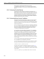
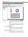
Installing/Running LoggerNet as a Service ..................................... 2-8
2.4.1 Issues with Running LoggerNet as a Service ............................ 2-9
2.4.1.1 Write Access .................................................................. 2-9
2.4.1.2 Network Drives ............................................................ 2-10
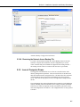
2.5
Special Note on Windows XP Service Pack 2 ............................... 2-10
3. Introduction .............................................................. 3-1
3.1
What is LoggerNet? ......................................................................... 3-1
3.1.1 What Next? ............................................................................... 3-1
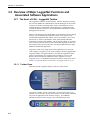
3.2
Overview of Major LoggerNet Functions and Associated
Software Applications .................................................................. 3-2
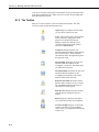
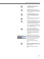
3.2.1 The Heart of it All – LoggerNet Toolbar .................................. 3-2
3.2.1.1 Toolbar Views ................................................................ 3-2
3.2.1.2 Favorites Category ......................................................... 3-3
3.2.1.3 Toolbar Menus ............................................................... 3-4
3.2.1.4 Command Line Arguments ............................................ 3-4
3.2.1.5 Alternate Language Support ........................................... 3-5
3.2.2 LoggerNet Admin/LoggerNet Remote ..................................... 3-6
3.2.3 Setting Up Datalogger Communication Networks.................... 3-6
3.2.4 Real Time Tools........................................................................ 3-7
3.2.5 Network Status and Problem Solving ....................................... 3-7
3.2.6 Network Management Tools..................................................... 3-8
3.2.7 Creating and Editing Datalogger Programs .............................. 3-8
3.2.8 Working with Data Files ........................................................... 3-9
3.2.9 Automating Tasks with Task Master ...................................... 3-10
3.2.10 Managing External Data Storage Devices .............................. 3-10
i
Table of Contents
3.2.11 Optional Client Products Compatible with LoggerNet ........... 3-10
3.2.11.1 LoggerNetData ............................................................. 3-10
3.2.11.2 Data Display Clients ..................................................... 3-11
3.2.11.3 Baler ............................................................................. 3-11
3.2.11.4 CSIOPC Server (PC-OPC) ........................................... 3-11
3.2.11.5 Software Development Kit ........................................... 3-11
3.3
Getting Help for LoggerNet Applications ...................................... 3-11
4. Setting up Datalogger Networks ............................ 4-1
4.1
4.2
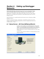
Setup Screen – EZ View (EZSetup Wizard) .................................... 4-1
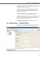
Setup Screen — Standard View ....................................................... 4-3
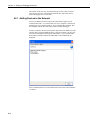
4.2.1 Adding Devices to the Network ................................................ 4-4
4.2.2 Applying Changes, Undo and Redo .......................................... 4-6
4.2.3 Renaming Network Devices...................................................... 4-7
4.2.4 Device Settings ......................................................................... 4-7
4.2.4.1 ComPort.......................................................................... 4-7
4.2.4.2 IPPort (Internet Protocol Serial Port).............................. 4-8
4.2.4.3 TAPIPort (Telephony API)............................................. 4-9
4.2.4.4 Datalogger or Recording Device .................................. 4-11
4.2.4.4.1 Hardware Tab .................................................... 4-11
4.2.4.4.2 Schedule Tab ..................................................... 4-13
4.2.4.4.3 Final Storage Area 1 and 2 Tab (Edlog
Dataloggers with Mixed-array Operating
System) ........................................................... 4-17
4.2.4.4.4 Data Files Tab (CRBasic Dataloggers, and
Edlog Dataloggers with Table Data and
PakBus Operating systems) ............................ 4-18
4.2.4.4.5 Clock Tab .......................................................... 4-21
4.2.4.4.6 Program Tab ...................................................... 4-22
4.2.4.4.7 File Retrieval Tab (CR1000, CR3000,
CR800 Series, CR6 Series, and Edlog
Dataloggers with PakBus Operating
Systems) ......................................................... 4-22
4.2.4.5 PhoneBase .................................................................... 4-23
4.2.4.6 PhoneRemote ................................................................ 4-24
4.2.4.7 RFBase ......................................................................... 4-25
4.2.4.8 RFRemote ..................................................................... 4-26
4.2.4.9 RFBase-TD ................................................................... 4-27
4.2.4.10 RF RemoteTD .............................................................. 4-31
4.2.4.11 RFRemote-PB............................................................... 4-31
4.2.4.12 MD9 Base ..................................................................... 4-32
4.2.4.13 MD9 Remote ................................................................ 4-34
4.2.4.14 RF400 ........................................................................... 4-35
4.2.4.15 RF400 Remote .............................................................. 4-36
4.2.4.16 Generic Modem ............................................................ 4-38
4.2.4.17 PakBusPort ................................................................... 4-39
4.2.4.18 PakBus Router .............................................................. 4-42
4.2.4.19 PakBusPort HD ............................................................ 4-43
4.2.4.20 PakBusTcpServer ......................................................... 4-44
4.2.4.21 SerialPortPool ............................................................... 4-46
4.2.4.22 TerminalPortPool.......................................................... 4-49
4.2.5 Setting Up Scheduled Data Collection .................................... 4-52
4.2.5.1 Data Collection Scheduling Considerations ................. 4-52
4.2.5.2 Intervals ........................................................................ 4-53
4.2.5.2.1 Datalogger Program Intervals ............................ 4-53
ii
Table of Contents
4.2.5.2.2 Data Collection Setting Intervals ....................... 4-53
4.2.5.2.3 Communications Path Considerations ............... 4-54
4.2.5.3 Setting Up Scheduled Data Collection ......................... 4-54
4.2.6 Setting the Clock ..................................................................... 4-56
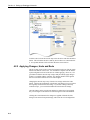
4.2.7 Sending a Program to the Datalogger from Setup................... 4-57
4.2.8 Setup’s Tools Menu ................................................................ 4-57
4.2.8.1 LoggerNet Server Settings ........................................... 4-57
4.2.8.1.1 LoggerNet Settings ............................................ 4-57
4.2.8.1.2 PakBus Settings ................................................. 4-58
4.2.8.1.3 LoggerNet Defaults ........................................... 4-58
4.2.8.1.4 IPManager Settings ........................................... 4-58
4.2.8.2 Copy Device Settings ................................................... 4-59
4.2.8.3 Troubleshooter ............................................................. 4-60
4.2.9 Setup’s Backup Menu ............................................................. 4-60
4.2.10 Selecting a Remote Server ...................................................... 4-60
4.2.11 Selecting a View ..................................................................... 4-60
4.3
Network Planner ............................................................................ 4-62
4.3.1 Functional Overview............................................................... 4-62
4.3.2 The Drawing Canvas .............................................................. 4-62
4.3.2.1 Adding a Background Image ........................................ 4-63
4.3.2.2 Scrolling the Drawing Canvas ...................................... 4-63
4.3.2.3 Changing the Canvas Scale .......................................... 4-65
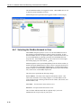
4.3.3 Adding Stations to the Network .............................................. 4-65
4.3.4 Adding Peripherals to a Station .............................................. 4-65
4.3.5 Adding Stations Links............................................................. 4-66
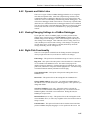
4.3.6 Adding Activities .................................................................... 4-68
4.3.7 The Station Summary ............................................................. 4-71
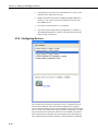
4.3.8 Configuring Devices ............................................................... 4-72
4.3.8.1 Configuring Using the Device Configuration
Protocol .................................................................... 4-73
4.3.8.1.1 Avoiding Conflicts with the LoggerNet
Server ............................................................. 4-74
4.3.8.1.2 Settings Generated ............................................. 4-75
4.3.8.2 Configuring a LoggerNet Server .................................. 4-75
4.3.9 Saving Your Work .................................................................. 4-78
4.3.10 Arranging Screen Components ............................................... 4-79
4.4
Device Configuration Utility.......................................................... 4-79
5. Real-Time Tools ....................................................... 5-1
5.1
The Connect Screen ......................................................................... 5-1
5.1.1 Connecting to the Datalogger — or Not ................................... 5-1
5.1.2 Data Collection ......................................................................... 5-3
5.1.2.1 Collect Now ................................................................... 5-3
5.1.2.2 Custom Collection .......................................................... 5-4
5.1.2.2.1 Mixed-array Dataloggers ..................................... 5-4
5.1.2.2.2 Table-based Dataloggers ..................................... 5-5
5.1.3 Ports and Flags .......................................................................... 5-8
5.1.4 Datalogger Clock .................................................................... 5-10
5.1.5 Program Management ............................................................. 5-10
5.1.5.1 Sending a Datalogger Program..................................... 5-11
5.1.5.2 CR200 Series Programs................................................ 5-11
5.1.5.3 Retrieving Datalogger Programs .................................. 5-11
5.1.6 Program Association ............................................................... 5-12
5.1.7 Data Displays .......................................................................... 5-12
5.1.7.1 Data Display Limitations.............................................. 5-13
iii
Table of Contents
5.1.7.2 Numeric Display Screens ............................................. 5-14
5.1.7.2.1 Adding and Removing Values ........................... 5-14
5.1.7.2.2 Display Options ................................................. 5-16
5.1.7.2.3 Right Click Menu Options ................................. 5-17
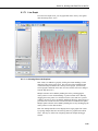
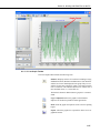
5.1.7.3 Graphical Display Screens............................................ 5-17
5.1.7.3.1 Displaying Values on a Graph ........................... 5-18
5.1.7.3.2 Graph Options.................................................... 5-19
5.1.7.3.3 Trace Options .................................................... 5-24
5.1.7.3.4 Right Click Menu Options ................................. 5-25
5.1.7.3.5 Additional Capabilities ...................................... 5-27
5.1.8 Table Monitor ......................................................................... 5-27
5.1.9 File Control for CR5000, CR1000, CR800 Series, CR6
Series, CR3000, and CR9000 Dataloggers .......................... 5-27
5.1.10 Terminal Emulator .................................................................. 5-32
5.1.11 Station Status........................................................................... 5-32
5.1.12 Calibration Wizard .................................................................. 5-34
5.2
Real-Time Monitoring and Control ................................................ 5-34
5.2.1 Development Mode ................................................................. 5-35
5.2.1.1 The RTMC Workspace ................................................. 5-36
5.2.1.2 Display Components..................................................... 5-36
5.2.1.3 Functions Available from the RTMC Menus ............... 5-38
5.2.1.4 Expressions ................................................................... 5-43
5.2.1.4.1 Operators ........................................................... 5-45
5.2.1.4.2 Order of Precedence .......................................... 5-46
5.2.1.4.3 Predefined Constants ......................................... 5-46
5.2.1.4.4 Predefined Time Constants ................................ 5-46
5.2.1.4.5 Functions ........................................................... 5-47
5.2.1.4.6 Logical Functions .............................................. 5-48
5.2.1.4.7 String Functions ................................................. 5-49
5.2.1.4.8 Conversion Functions ........................................ 5-49
5.2.1.4.9 Time Functions .................................................. 5-50
5.2.1.4.10 Start Option Functions ....................................... 5-50
5.2.1.4.11 Statistical Functions ........................................... 5-51
5.2.1.5 Remote Connection ...................................................... 5-52
5.2.2 RTMC Run-Time .................................................................... 5-52
6. Network Status and Resolving Communication
Problems ............................................................... 6-1
6.1
Status Monitor .................................................................................. 6-1
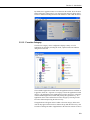
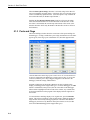
6.1.1 Visual Status Indicators............................................................. 6-2
6.1.2 Status Monitor Functions .......................................................... 6-3
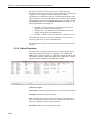
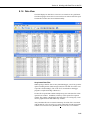
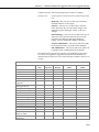
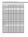
6.1.2.1 Selecting Columns .......................................................... 6-3
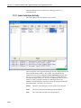
6.1.2.2 Display/Subnet ............................................................... 6-8
6.1.2.3 Toggle Collection On/Off ............................................... 6-8
6.1.2.4 Reset Device ................................................................... 6-8
6.1.2.5 Collect Now/Stop Collection .......................................... 6-8
6.1.2.6 Pool Statistics ................................................................. 6-9
6.1.2.7 Pool Devices ................................................................... 6-9
6.1.2.8 State of Operations ....................................................... 6-10
6.2
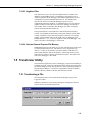
LogTool .......................................................................................... 6-12
6.2.1 Log Types ............................................................................... 6-12
6.2.2 Using LogTool ........................................................................ 6-12
6.2.3 Saving Logs to File ................................................................. 6-13
iv
Table of Contents
6.3
6.4
Comm Test ..................................................................................... 6-14
PakBus Graph ................................................................................ 6-15
6.4.1 Selecting the PakBus Network to View .................................. 6-16
6.4.2 Dynamic and Static Links ....................................................... 6-17
6.4.3 Viewing/Changing Settings in a PakBus Datalogger .............. 6-17
6.4.4 Right-Click Functionality ....................................................... 6-17
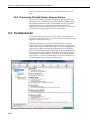
6.4.5 Discovering Probable Routes between Devices ...................... 6-18
6.5
Troubleshooter ............................................................................... 6-18
6.5.1 Status Information................................................................... 6-19
6.5.2 Buttons .................................................................................... 6-19
6.5.3 TD-RF Test ............................................................................. 6-20
6.5.3.1 RF Link Quality Test.................................................... 6-23
6.5.3.2 TD-RF Quality Report.................................................. 6-23
6.5.3.3 Advanced Features ....................................................... 6-26
6.5.4 Archiving Troubleshooter Results .......................................... 6-26
6.5.5 Other Tools in Troubleshooter ................................................ 6-27
6.6
LoggerNet Server Monitor ............................................................. 6-27
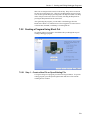
7. Creating and Editing Datalogger Programs .......... 7-1
7.1
7.2
Review of CSI Datalogger Models .................................................. 7-1
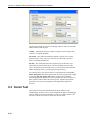
Short Cut .......................................................................................... 7-2
7.2.1 Overview................................................................................... 7-2
7.2.2 Creating a Program Using Short Cut ........................................ 7-3
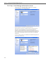
7.2.2.1 Step 1 – Create a New File or Open Existing File.......... 7-3
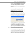
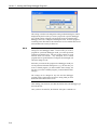
7.2.2.2 Step 2 – Select Datalogger and Specify Scan Interval ... 7-4
7.2.2.3 Step 3 – Choose Sensors to Monitor .............................. 7-7
7.2.2.4 Step 4 – Setup Output Tables ....................................... 7-14
7.2.2.5 Step 5 – Generate the Program in the Format
Required by the Datalogger ...................................... 7-17
7.2.3 Short Cut Settings ................................................................... 7-18
7.2.3.1 Program Security .......................................................... 7-18
7.2.3.2 Datalogger ID ............................................................... 7-18
7.2.3.3 Power-up Settings ........................................................ 7-18
7.2.3.4 Select CR200 Compiler ................................................ 7-19
7.2.3.5 Sensor Support ............................................................. 7-19
7.2.3.6 Integration/First Notch Frequency (fN1) ....................... 7-20
7.2.3.7 Font .............................................................................. 7-20
7.2.3.8 Set Working Directory ................................................. 7-20
7.2.3.9 Enable Creation of Custom Sensor Files ...................... 7-20
7.2.4 Editing Programs Created by Short Cut .................................. 7-20
7.2.5 New Sensor Files .................................................................... 7-21
7.2.6 Custom Sensor Files ............................................................... 7-21
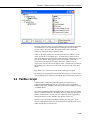
7.3
CRBasic Editor .............................................................................. 7-21
7.3.1 Overview................................................................................. 7-21
7.3.2 Inserting Instructions .............................................................. 7-22
7.3.2.1 Parameter Dialog Box .................................................. 7-22
7.3.2.2 Right-Click Functionality ............................................. 7-24
7.3.3 Toolbar .................................................................................... 7-25
7.3.3.1 Compile ........................................................................ 7-27
7.3.3.2 Compile, Save, and Send .............................................. 7-27
7.3.3.3 Conditional Compile and Save ..................................... 7-31
7.3.3.4 Templates ..................................................................... 7-31
7.3.3.5 Program Navigation using BookMarks and GoTo ....... 7-32
7.3.3.6 CRBasic Editor File Menu ........................................... 7-32
7.3.3.7 CRBasic Editor Edit Menu ........................................... 7-33
v
Table of Contents
7.3.3.7.1 Other Options .................................................... 7-33
7.3.3.8 CRBasic Editor View Menu ......................................... 7-33
7.3.3.8.1 Editor Preferences .............................................. 7-33
7.3.3.8.2 Instruction Panel Preferences............................. 7-35
7.3.3.8.3 Other Options .................................................... 7-35
7.3.3.9 CRBasic Editor Tools Menu ......................................... 7-36
7.3.3.9.1 Edit Instruction Categories ................................ 7-36
7.3.3.9.2 Constant Customization ..................................... 7-37
7.3.3.9.3 Other Options .................................................... 7-39
7.3.3.10 Available Help Information .......................................... 7-40
7.3.4 CRBasic Programming............................................................ 7-40
7.3.4.1 Programming Sequence ................................................ 7-40
7.3.4.2 Program Declarations ................................................... 7-41
7.3.4.3 Mathematical Expressions ............................................ 7-42
7.3.4.4 Measurement and Output Processing Instructions ........ 7-42
7.3.4.5 Line Continuation ......................................................... 7-43
7.3.4.6 Inserting Comments Into Program................................ 7-43
7.3.4.7 Example Program ......................................................... 7-44
7.3.4.8 Data Tables ................................................................... 7-44
7.3.4.9 The Scan — Measurement Timing and Processing ...... 7-46
7.3.4.10 Numerical Entries ......................................................... 7-47
7.3.4.11 Logical Expression Evaluation ..................................... 7-47
7.3.4.11.1 What is True?..................................................... 7-47
7.3.4.11.2 Expression Evaluation ....................................... 7-48
7.3.4.11.3 Numeric Results of Expression Evaluation ....... 7-48
7.3.4.12 Flags ............................................................................. 7-49
7.3.4.13 Parameter Types ........................................................... 7-49
7.3.4.13.1 Expressions in Parameters ................................. 7-49
7.3.4.13.2 Arrays of Multipliers and Offsets for Sensor
Calibration ...................................................... 7-50
7.3.4.14 Program Access to Data Tables .................................... 7-50
7.4
Edlog .............................................................................................. 7-51
7.4.1 Overview ................................................................................. 7-51
7.4.1.1 Precompiler................................................................... 7-51
7.4.1.2 Context-sensitive Help ................................................. 7-52
7.4.1.3 Programming Efficiency............................................... 7-52
7.4.1.4 Input Location Labels ................................................... 7-52
7.4.1.5 Final Storage Label Editor ............................................ 7-52
7.4.1.6 Expression Compiler .................................................... 7-52
7.4.2 Creating a New Edlog Program .............................................. 7-53
7.4.2.1 Program Structure ......................................................... 7-54
7.4.2.2 Edlog File Types........................................................... 7-55
7.4.2.3 Inserting Instructions into the Program ........................ 7-56
7.4.2.4 Entering Parameters for the Instructions ...................... 7-57
7.4.2.5 Program Comments ...................................................... 7-57
7.4.2.6 Expressions ................................................................... 7-58
7.4.2.7 Editing an Existing Program......................................... 7-63
7.4.2.8 Editing Comments, Instructions, and Expressions ....... 7-65
7.4.2.9 Cut, Copy, Paste, and Clipboard Options ..................... 7-65
7.4.3 Library Files ............................................................................ 7-65
7.4.4 Documenting a DLD File ........................................................ 7-65
7.4.5 Display Options....................................................................... 7-66
7.4.5.1 Graphical Toolbar ......................................................... 7-66
7.4.5.2 Renumbering the Instructions ....................................... 7-67
7.4.5.3 Compress VIEW ........................................................... 7-67
7.4.5.4 Indention ....................................................................... 7-67
vi
Table of Contents
7.4.6 Input Locations ....................................................................... 7-67
7.4.7 Entering Input Locations......................................................... 7-68
7.4.8 Repetitions .............................................................................. 7-68
7.4.9 Input Location Editor .............................................................. 7-69
7.4.10 Input Location Anomalies....................................................... 7-70
7.4.11 Final Storage Labels ............................................................... 7-71
7.4.12 Datalogger Settings Stored in the DLD File ........................... 7-73
7.4.13 Program Security .................................................................... 7-73
7.4.13.1 Setting Passwords in the DLD...................................... 7-73
7.4.13.2 Disabling Passwords .................................................... 7-73
7.4.14 Final Storage Area 2 ............................................................... 7-74
7.4.15 DLD File Labels ..................................................................... 7-74
7.4.15.1 Mixed-array Dataloggers .............................................. 7-74
7.4.15.2 Table-Based Dataloggers ............................................. 7-74
7.4.16 Power Up Settings/Compile Settings ...................................... 7-75
7.4.17 Datalogger Serial Port Settings ............................................... 7-75
7.4.18 PakBus Settings ...................................................................... 7-75
7.4.18.1 Network ........................................................................ 7-76
7.4.18.2 Beacon Intervals ........................................................... 7-76
7.4.18.3 Neighbor Filter ............................................................. 7-77
7.4.18.4 Allocate General Purpose File Memory ....................... 7-77
7.5
Transformer Utility ........................................................................ 7-77
7.5.1 Transforming a File ................................................................ 7-77
7.5.2 Controls................................................................................... 7-79
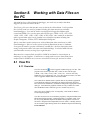
8. Working with Data Files on the PC......................... 8-1
8.1
View Pro .......................................................................................... 8-1
8.1.1 Overview................................................................................... 8-1
8.1.2 The Toolbar............................................................................... 8-2
8.1.3 Opening a File........................................................................... 8-4
8.1.3.1 Opening a Data File........................................................ 8-4
8.1.3.2 Opening Other Types of Files ........................................ 8-4
8.1.3.3 Opening a File in Hexadecimal Format.......................... 8-4
8.1.4 Viewing a LoggerNet Database Table ...................................... 8-4
8.1.4.1 Selecting a Database....................................................... 8-4
8.1.4.2 Selecting a Table ............................................................ 8-8
8.1.5 Importing a CSV File ................................................................ 8-8
8.1.6 Data View ............................................................................... 8-11
8.1.6.1 Column Size ................................................................. 8-12
8.1.6.2 Header Information ...................................................... 8-12
8.1.6.3 Row Shading ................................................................ 8-12
8.1.6.4 Locking the TimeStamp Column ................................. 8-12
8.1.6.5 File Information............................................................ 8-12
8.1.6.6 Background Color ........................................................ 8-12
8.1.6.7 Font .............................................................................. 8-12
8.1.6.8 Window Arrangement .................................................. 8-13
8.1.7 Graphs ..................................................................................... 8-13
8.1.7.1 Line Graph ................................................................... 8-15
8.1.7.1.1 Selecting Data to be Graphed ............................ 8-15
8.1.7.1.2 Graph Width ...................................................... 8-16
8.1.7.1.3 Scrolling ............................................................ 8-16
8.1.7.1.4 Graph Cursor ..................................................... 8-16
8.1.7.1.5 Line Graph Toolbar ........................................... 8-17
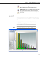
8.1.7.2 Histogram ..................................................................... 8-19
8.1.7.2.1 Selecting Data to be Viewed ............................. 8-20
vii
Table of Contents
8.1.7.2.2 Options............................................................... 8-21
8.1.7.2.3 Histogram Toolbar ............................................. 8-21
8.1.7.3 XY Plot ......................................................................... 8-22
8.1.7.3.1 Selecting Data to be Plotted ............................... 8-23
8.1.7.3.2 XY Plot Toolbar ................................................ 8-23
8.1.7.4 Rainflow Histogram ..................................................... 8-24
8.1.7.4.1 Selecting Data to be View ................................. 8-25
8.1.7.4.2 Options............................................................... 8-26
8.1.7.4.3 Rainflow Histogram Toolbar ............................. 8-26
8.1.7.5 FFT ............................................................................... 8-27
8.1.7.5.1 Selecting Data to be Graphed ............................ 8-28
8.1.7.5.2 Options............................................................... 8-29
8.1.7.5.3 FFT Toolbar ....................................................... 8-29
8.1.8 Right-click-Menus................................................................... 8-30
8.1.8.1 Data View ..................................................................... 8-30
8.1.8.2 Graphs .......................................................................... 8-32
8.1.8.3 Traces ........................................................................... 8-32
8.1.9 Printing Options ...................................................................... 8-32
8.1.9.1 Print Setup .................................................................... 8-32
8.1.9.2 Printing Text ................................................................. 8-33
8.1.9.3 Printing Graphs ............................................................. 8-33
8.1.10 View Pro Online Help ............................................................. 8-33
8.1.11 Assigning Data Files to View.................................................. 8-33
8.2
Split ................................................................................................ 8-33
8.2.1 Functional Overview ............................................................... 8-33
8.2.2 Getting Started ........................................................................ 8-34
8.2.3 Split Parameter File Entries..................................................... 8-40
8.2.3.1 Input Files ..................................................................... 8-40
8.2.3.1.1 File Info ............................................................. 8-41
8.2.3.1.2 File Offset/Options ............................................ 8-42
8.2.3.1.3 Start Condition ................................................... 8-45
8.2.3.1.4 Stop Condition ................................................... 8-47
8.2.3.1.5 Copy .................................................................. 8-51
8.2.3.1.6 Select ................................................................. 8-52
8.2.3.1.7 Ranges ............................................................... 8-52
8.2.3.1.8 Variables ............................................................ 8-53
8.2.3.1.9 Numerical Limitations ....................................... 8-54
8.2.3.1.10 Mathematical Functions, Details, and
Examples ........................................................ 8-54
8.2.3.1.11 Time Series Functions, Details, and Examples .. 8-56
8.2.3.1.12 Special Functions, Details, and Examples ......... 8-61
8.2.3.1.13 Split Functions Example .................................... 8-66
8.2.3.1.14 Summary of Select Line Syntax Rules .............. 8-68
8.2.3.1.15 Time Synchronization ........................................ 8-69
8.2.3.2 Output Files .................................................................. 8-72
8.2.3.2.1 Description of Output Option Commands ......... 8-73
8.2.3.2.2 Report Headings ................................................ 8-78
8.2.3.2.3 Column Headings .............................................. 8-78
8.2.4 Help Option ............................................................................. 8-78
8.2.5 Editing Commands .................................................................. 8-79
8.2.6 Running Split From a Command Line .................................... 8-79
8.2.6.1 Splitr Command Line Switches .................................... 8-79
8.2.6.1.1 Closing the Splitr.exe Program After
Execution (/R or /Q Switch) ........................... 8-79
8.2.6.1.2 Running Splitr in a Hidden or Minimized
State (/H Switch) ............................................ 8-79
viii
Table of Contents
8.2.6.1.3
Running Multiple Copies of Splitr (/M
Switch) ........................................................... 8-80
8.2.6.2 Using Splitr.exe in Batch Files ..................................... 8-80
8.2.6.3 Processing Alternate Files ............................................ 8-80
8.2.6.3.1 Input/Output File Command Line Switches
for Processing Alternate Files ........................ 8-81
8.2.6.4 Processing Multiple Parameter Files with One
Command Line ......................................................... 8-84
8.2.7 Log Files ................................................................................. 8-84
8.3
CardConvert ................................................................................... 8-84
8.3.1 Input/Output File Settings ....................................................... 8-85
8.3.2 Destination File Options ......................................................... 8-85
8.3.2.1 File Format ................................................................... 8-86
8.3.2.2 File Processing ............................................................. 8-86
8.3.2.3 File Naming .................................................................. 8-87
8.3.2.4 TOA5/TOB1 Format .................................................... 8-88
8.3.3 Converting the File ................................................................. 8-88
8.3.3.1 Repairing/Converting Corrupted Files ......................... 8-88
8.3.4 Viewing a Converted File ....................................................... 8-89
8.3.5 Running CardConvert From a Command Line ....................... 8-89
9. Automating Tasks with Task Master ...................... 9-1
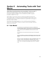
9.1
Task Master ...................................................................................... 9-1
9.1.1 Setup Tab .................................................................................. 9-2
9.1.1.1 Adding Tasks.................................................................. 9-2
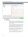
9.1.1.2 Logger Event Tasks ........................................................ 9-3
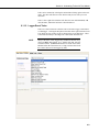
9.1.1.3 Scheduled Event Tasks................................................... 9-6
9.1.1.3.1 Interval Tasks ...................................................... 9-6
9.1.1.3.2 Calendar .............................................................. 9-7
9.1.1.4 Define What the Task Does............................................ 9-9
9.1.2 Status Tab ............................................................................... 9-14
9.1.3 Remote Administration of the Task Master ............................ 9-16
9.1.4 Task Master Logs.................................................................... 9-16
10. Utilities Installed with LoggerNet ......................... 10-1
10.1 Device Configuration Utility.......................................................... 10-1
10.1.1 Overview................................................................................. 10-1
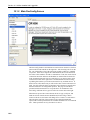
10.1.2 Main DevConfig Screen ......................................................... 10-2
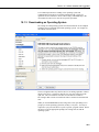
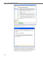
10.1.3 Downloading an Operating System ........................................ 10-3
10.1.4 Terminal Tab........................................................................... 10-5
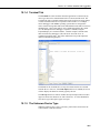
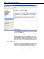
10.1.5 The Unknown Device Type .................................................... 10-5
10.1.6 Off-line Mode ......................................................................... 10-6
10.2 CoraScript ...................................................................................... 10-7
10.2.1 CoraScript Fundamentals ........................................................ 10-7
10.2.2 Useful CoraScript Operations ................................................. 10-7
10.2.2.1 Connecting to the LoggerNet Server ............................ 10-8
10.2.2.2 Checking and Setting Device Settings ......................... 10-8
10.2.2.3 Creating and using a Network Backup File .................. 10-8
10.2.2.4 Hole Management ........................................................ 10-9
10.2.2.5 Scripting CoraScript Commands ................................ 10-10
10.3 RWIS Administrator .................................................................... 10-10
10.3.1 Overview............................................................................... 10-10
10.3.2 Adding a New RWIS Station ................................................ 10-11
10.3.3 Editing Station Settings......................................................... 10-12
ix
Table of Contents
10.3.3.1 Station Communication Settings ................................ 10-12
10.3.3.2 Schedule Settings........................................................ 10-13
10.3.3.3 Snapshots Settings ...................................................... 10-15
10.3.3.4 Clock Settings ............................................................. 10-16
10.3.3.5 Data Tab ..................................................................... 10-18
10.3.4 Deleting a Station .................................................................. 10-18
10.3.5 Organization of RWIS Data in LoggerNet ............................ 10-18
10.4 File Format Convert ..................................................................... 10-19
10.4.1 Overview ............................................................................... 10-19
10.4.2 Options .................................................................................. 10-20
10.5 Toa_to_tob1 ................................................................................. 10-22
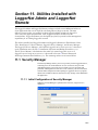
11. Utilities Installed with LoggerNet Admin and
LoggerNet Remote .............................................. 11-1
11.1 Security Manager ........................................................................... 11-1
11.1.1 Initial Configuration of Security Manager .............................. 11-1
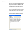
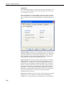
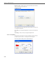
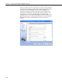
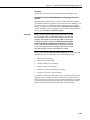
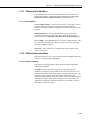
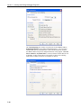
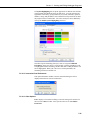
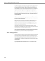
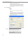
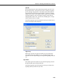
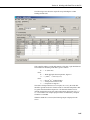
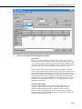
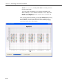
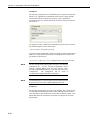
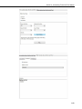
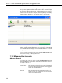
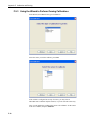
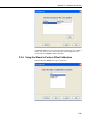
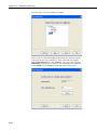
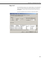
11.1.2 Managing User Accounts ........................................................ 11-2
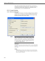
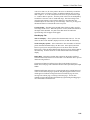
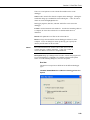
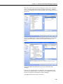
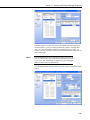
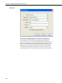
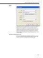
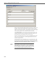
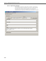
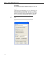
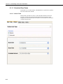
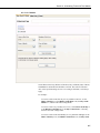
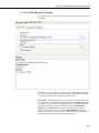
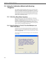
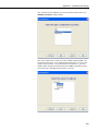
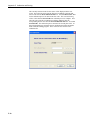
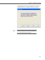
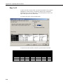
Adding an Account ....................................................................... 11-2
Deleting an Account ..................................................................... 11-5
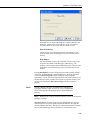
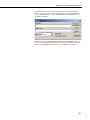
Editing a Password ....................................................................... 11-5
Changing Security Levels ............................................................. 11-5
Special Access .............................................................................. 11-5
11.1.3 Resetting Security ................................................................... 11-5
11.1.4 Remote Task Management ...................................................... 11-5
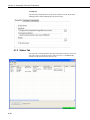
11.2 Hole Monitor .................................................................................. 11-5
11.2.1 Hole Collection Activity ......................................................... 11-6
11.2.2 Message Log ........................................................................... 11-7
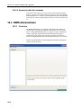
11.3 Data Filer ........................................................................................ 11-8
11.3.1 Data Filer Requirements.......................................................... 11-8
11.3.2 Using the Data Filer ................................................................ 11-8
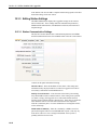
11.3.2.1 Connecting to a Computer Running the LoggerNet
Server Software......................................................... 11-8
11.3.2.1.1 Setting Up the Data Filer ................................... 11-9
11.3.2.2 Collection Options ........................................................ 11-9
11.3.3 The Collected Data ................................................................ 11-11
11.3.4 Determining the Data Available in the Data Cache .............. 11-11
11.3.5 Record Number Anomalies ................................................... 11-12
11.3.6 Communication Status .......................................................... 11-12
11.4 Data Export .................................................................................. 11-12
11.4.1 Functional Overview ............................................................. 11-12
11.4.2 Theory of Operation .............................................................. 11-14
11.4.3 Custom Data Retrieval Client ............................................... 11-15
11.4.4 Custom Client/Data Export Interface Description................. 11-15
11.4.5 RTMS Format Description .................................................... 11-20
11.4.6 Standard Format Description ................................................ 11-21
12. Optional Client Applications Available for
LoggerNet ............................................................ 12-1
12.1
12.2
12.3
12.4
12.5
Allowing Remote Connections to the LoggerNet Server ............... 12-1
LoggerNetData ............................................................................... 12-1
RTMC Run-Time ........................................................................... 12-2
RTMC Pro ...................................................................................... 12-2
LNDB ............................................................................................. 12-2
x
Table of Contents
12.6
12.7
12.8
Baler ............................................................................................... 12-2
CSIOPC Server (PC-OPC)............................................................. 12-3
Software Development Kit............................................................. 12-3
13. Implementing Advanced Communications
Links ..................................................................... 13-1
13.1 Phone to RF.................................................................................... 13-1
13.1.1 Setup ....................................................................................... 13-1
13.1.2 Operational Considerations ..................................................... 13-2
13.1.2.1 Scheduled Data Collection ........................................... 13-2
13.1.2.2 Extra Response Time.................................................... 13-2
13.1.2.3 RF Address ................................................................... 13-2
13.1.2.4 Max Time Online ......................................................... 13-2
13.1.3 Attaching a Datalogger to the RF Base ................................... 13-2
13.1.3.1 Hardware Setup ............................................................ 13-3
13.1.3.2 Network Setup in LoggerNet ....................................... 13-3
13.2 Phone to MD9 ................................................................................ 13-3
13.2.1 Setup ....................................................................................... 13-3
13.2.2 Operational Considerations ..................................................... 13-4
13.2.2.1 Scheduled Data Collection ........................................... 13-4
13.2.2.2 MD9 Addresses ............................................................ 13-4
13.2.2.3 Extra Response Time.................................................... 13-4
13.2.2.4 Max Time Online ......................................................... 13-4
13.2.2.5 Grounding .................................................................... 13-5
13.3 TCP/IP to RF.................................................................................. 13-5
13.3.1 Setup ....................................................................................... 13-5
13.3.2 Operational Considerations ..................................................... 13-5
13.3.3 Special Considerations ............................................................ 13-6
14. Troubleshooting Guide ......................................... 14-1
14.1 What’s Changed? ........................................................................... 14-1
14.2 LoggerNet Server Problems ........................................................... 14-1
14.2.1 Starting LoggerNet and Connecting to the Server .................. 14-1
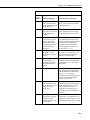
14.2.2 Socket Errors........................................................................... 14-2
14.2.3 Data Collection Issues............................................................. 14-4
14.3 Application Screen Problems ......................................................... 14-4
14.4 General Communication Link Problems ........................................ 14-4
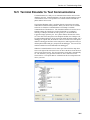
14.5 Terminal Emulator to Test Communications ................................. 14-5
14.6 RF Communication Link Issues ..................................................... 14-8
14.6.1 Checking RF Components and Connections........................... 14-9
14.6.2 RF Signal Strength Testing ..................................................... 14-9
14.6.3 Troubleshooting with Attenuation Pads ................................ 14-11
14.7 Using Data Table Monitor ........................................................... 14-13
14.8 Troubleshooting PakBus Communications .................................. 14-17
Appendices
A. Glossary of Terms .................................................. A-1
B. Campbell Scientific File Formats .......................... B-1
B.1
PC File Data Formats ....................................................................... B-1
B.1.1 Comma Separated ..................................................................... B-1
xi
Table of Contents
B.1.2 ASCII Printable ........................................................................ B-2
B.1.3 TOACI1 ................................................................................... B-2
B.1.3.1 Field Name Suffixes ...................................................... B-3
B.1.4 TOA5 ....................................................................................... B-4
B.1.5 TOB1........................................................................................ B-4
B.1.6 Array Compatible CSV ............................................................ B-6
B.1.7 CSIXML................................................................................... B-6
B.1.7.1 A Short Introduction to XML ........................................ B-7
B.1.7.2 File Syntax ..................................................................... B-8
B.1.7.3 The csixml Element ..................................................... B-10
B.1.7.3.1 The head Element ................................................ B-10
B.1.7.3.2 The data Element ................................................. B-12
B.1.7.4 File Example ................................................................ B-13
B.1.8 CSIJSON ................................................................................ B-14
B.1.8.1 A Short Introduction to JSON ..................................... B-14
B.1.8.2 File Syntax ................................................................... B-15
B.1.8.2.1 The head Object ................................................... B-15
B.1.8.2.2 The data Array ..................................................... B-17
B.1.8.3 File Example ................................................................ B-17
B.2
Datalogger Data Formats............................................................... B-18
B.2.1 TOB2 or TOB3 ...................................................................... B-18
B.3
Binary Data Value Types .............................................................. B-20
B.3.1 FP2 (2 Byte Low Resolution Format) .................................... B-20
B.3.2 FP4 (4 Byte High Resolution Format) ................................... B-20
B.3.3 IEEE4 ..................................................................................... B-20
B.3.4 IEEE8 ..................................................................................... B-20
B.4
Converting Binary File Formats .................................................... B-20
B.4.1 Split ........................................................................................ B-21
B.4.2 View Pro ................................................................................ B-21
B.4.3 CardConvert ........................................................................... B-21
B.4.4 File Format Convert ............................................................... B-21
B.4.5 TOB32.EXE ........................................................................... B-21
B.5
RTMS Format Description ............................................................ B-21
C. Table-Based Dataloggers ....................................... C-1
C.1
Memory Allocation for Final Storage ............................................. C-1
C.1.1 CR10X-TD Family Table-Based Dataloggers ......................... C-1
C.1.2 CR5000/CR1000/CR6 Series/CR3000/CR800/CR9000
Memory for Programs and Data Storage .............................. C-2
C.1.3 CR200 Series Dataloggers ....................................................... C-2
C.2
Converting an Array-Based Program to a CR10X-TD TableBased Program using Edlog ......................................................... C-3
C.2.1 Steps for Program Conversion ................................................. C-3
C.2.2 Program Instruction Changes ................................................... C-4
C.3
Table Data Overview....................................................................... C-5
C.4
Default Tables ................................................................................. C-6
D. Software Organization ............................................ D-1
D.1
D.2
LoggerNet/Client Architecture ........................................................ D-1
LoggerNet Server Data Cache ......................................................... D-1
D.2.1 Organization ............................................................................. D-1
D.2.2 Operation .................................................................................. D-1
D.2.3 Retrieving Data from the Cache ............................................... D-2
D.2.4 Updating Table Definitions ...................................................... D-2
xii
Table of Contents
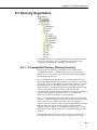
D.3
Directory Organization ................................................................... D-3
D.3.1 C:\CampbellSci Directory (Working Directory) ...................... D-3
D.3.2 C:\Program Files\CampbellSci\LoggerNet Directory
(Program File Directory) ...................................................... D-4
E. Log Files .................................................................. E-1
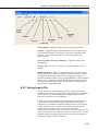
E.1
Event Logging .................................................................................. E-1
E.1.1 Log Categories .......................................................................... E-1
E.1.2 Enabling Log Files .................................................................... E-2
E.1.3 Log File Message Formats ........................................................ E-2
E.1.3.1 General File Format Information.................................... E-2
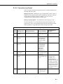
E.1.3.2 Transaction Log Format ................................................. E-3
E.1.3.3 Communications Status Log Format ............................ E-18
E.1.3.4 Object State Log Format .............................................. E-21
E.2
CQR Log (RF Link) ....................................................................... E-22
F. Calibration and Zeroing.......................................... F-1
F.1
F.2
F.3
F.4
F.5
F.6
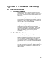
Calibration Essentials ....................................................................... F-1
F.1.1 Definition of Calibration ........................................................... F-1
F.1.2 Basic Calibration Process ......................................................... F-1
Writing Calibration Programs with the CRBasic Editor .................. F-2
F.2.1 The FieldCal Instruction ........................................................... F-2
F.2.2 Calibration File Details ............................................................. F-3
Four Kinds of Calibration ................................................................ F-3
F.3.1 Zeroing ...................................................................................... F-3
F.3.2 Offset Calibration ..................................................................... F-4
F.3.3 Two-Point Multiplier and Offset Calibration ............................ F-4
F.3.4 Two-Point Multiplier Only Calibration .................................... F-5
Performing a Manual Calibration..................................................... F-5
F.4.1 How to Use the Mode Variable for Calibration Status
and Control ............................................................................ F-5
F.4.2 Using the Mode Variable for Manual Single-Point
Calibration ............................................................................. F-6
F.4.3 Using the Mode Variable for Manual Two-Point Calibration .. F-7
Using the Calibration Wizard with Running Programs .................... F-8
F.5.1 Calibration Wizard Basic Operation ......................................... F-8
F.5.2 Using the Wizard to Perform Two-Point Multiplier and
Offset Calibrations ................................................................ F-8
F.5.3 Using the Wizard to Perform Zeroing Calibrations ................ F-12
F.5.4 Using the Wizard to Perform Offset Calibrations ................... F-13
Strain and Shunt Calibration .......................................................... F-15
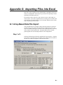
G. Importing Files into Excel ...................................... G-1
G.1
G.2
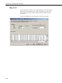
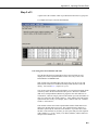
Array-Based Data File Import ......................................................... G-1
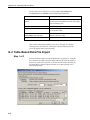
Table-Based Data File Import ......................................................... G-4
7-1.
7-2.
7-3.
7-4.
7-5.
Formats for Output Data ................................................................ 7-46
Formats for Entering Numbers in CRBasic ................................... 7-47
Synonyms for True and False ........................................................ 7-48
Rules for Names ............................................................................. 7-49
Operators and Functions ................................................................ 7-59
Tables
xiii
Table of Contents
7-6.
8-1.
Editor Keystrokes ........................................................................... 7-64
Comma Separated, Field Formatted, Printable ASCII, and
Table Oriented ASCII Input File Format Types ......................... 8-40
8-2. Example of Event Driven Test Data Set......................................... 8-49
8-3. Processed Data File Using Option C .............................................. 8-50
8-4. Input File Entries to Process the First Data Point for each Test ..... 8-51
8-5. Effects of Out of Range Values for Given Output Options ............ 8-53
8-6. Split Operators and Math Functions ............................................... 8-54
8-7. Time Series Functions .................................................................... 8-56
8-8. Split SPECIAL FUNCTIONS ........................................................ 8-61
8-9. Definition of Blank or Bad Data for each Data File Format .......... 8-75
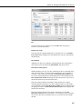
11-1. Security Manager Access Table ..................................................... 11-3
14-1. Socket Error Messages ................................................................... 14-3
B-1. Output Instruction Suffixes ............................................................. B-3
B-2. Pre-Defined XML Entities .............................................................. B-7
B-3. Field Data Types ........................................................................... B-11
C-1. Example of Status Table Entries (CR10T) ...................................... C-7
E-1. Transaction Log Messages ............................................................... E-3
E-2. Communication Status Log Messages............................................ E-19
F-1. The FieldCal Instruction “Family” ................................................... F-2
xiv
Preface — What’s New in LoggerNet 4?
Product History
LoggerNet 4 continues the original design of client-server functionality that
first appeared when Version 1.0 was released for Windows to replace Real
Time Monitoring Software (RTMS) that ran on OS/2 operating systems.
Versions in the 1.x series supported only table-based dataloggers and provided
large network users with sophisticated capabilities to develop clients to the
server to move data without having to store it in interim files.
Version 2.0 added support for dataloggers with mixed-array operating systems,
the CRBasic dataloggers, and additional communications devices. It also
supported client applications’ requests for data via TCP/IP, and automatically
created files on the PC for final storage data. Subsequent revisions in the 2.x
series added support for hardware as it was released and refined the clientserver architecture to make it more robust and flexible. Software development
kits and standalone clients were released to provide additional functionality.
One of the main efforts in the development of LoggerNet 3.1 was to
incorporate support for the CR1000 datalogger. This included datalogger
management (connect, collect data, set clock, send program, etc.) in
LoggerNet, as well as programming support in CRBasic and Short Cut. To
help with creating CR1000 programs, a Transformer utility was developed to
convert existing CR10X Edlog programs to CR1000 CRBasic programs.
LoggerNet 3.2 added support for our new CR3000 datalogger. In addition,
LoggerNet Admin and LoggerNet Remote were developed, which provide
tools to support larger networks. These tools include security and remote
management capabilities, and the ability to run LoggerNet as a service.
LoggerNet 3.3 added support for the CR800 datalogger. A new file output
option was also added for table-based dataloggers. This CSV file format
option allows the creation of data files similar to those from mixed array
dataloggers.
LoggerNet 3.4 improved LoggerNet’s performance on Windows Vista. In
addition, changes were made to the user interface of the Numeric Display and
Graphs.
NOTE
Beginning with LoggerNet 3.4, Windows NT is no longer
supported.
LoggerNet 4.0 introduces a new look and feel to the LoggerNet Toolbar.
Applications are divided into categories to make navigating the Toolbar easier.
You can also organize a Favorites category for the applications that you use
most often. A new file viewing application, View Pro, is introduced which
allows multiple data files to be opened, multiple graphs to be created, and
graphing in a variety of formats (Line Graph, X-Y Plot, Histogram, Rainflow
Histogram, and FFT). Another new application, the Network Planner, is
included. This is a graphical application that assists the user in designing
PakBus datalogger networks. It allows the development of a model of the
xv
Preface — What’s New in LoggerNet 4?
PakBus network, proposes and verifies valid connections between devices, and
allows integration of the model directly into LoggerNet 4.0.
See below for more details on what is new in LoggerNet 4.0 and each
individual application.
One of the main efforts in the development of LoggerNet 4.1 was the ability to
use LNDB databases with View Pro. The ability to lock the timestamp column
on the left of the data file has also been added to View Pro. This keeps the
timestamp visible as you scroll through columns of data. The Device
Configuration Utility adds an off-line mode which allows you to look at the
settings for a certain device type without actually being connected to a device.
The CRBasic Editor now has the capability to open a read-only copy of any
file. This gives you the ability to open multiple copies of a program and
examine multiple areas of a very large program at the same time. You can also
now continue an instruction onto multiple lines by placing the line continuation
indicator (a single space followed by an underscore “_”) at the end of the each
line that is to be continued. Also, bookmarks in a CRBasic program are now
persistent from session to session. In the Troubleshooter and the Setup Screen
(Standard View), you can now click on a potential problem to bring up a menu
that allows you to go the Setup Screen or Status Monitor to fix the potential
problem, bring up help describing the problem, or in some cases fix the
problem directly. Campbell Scientific’s new wireless sensors have been added
to the Network Planner. An option to provide feedback on LoggerNet is now
available from the LoggerNet Toolbar’s Help menu.
NOTE
Beginning with LoggerNet 4.1, Windows 2000 is no longer
supported.
LoggerNet 4.2 adds support for IPv6 addresses. IPv6 addresses are written as
eight two-byte address blocks separated by colons and surrounded by brackets
(e.g., [2620:24:8080:8600:85a1:fcf2:2172:11bf]). Prior to LoggerNet 4.2, only
IPv4 addresses were supported. IPv4 addresses are written in dotted decimal
notation (e.g., 192.168.11.197). Leading zeroes are stripped for both IPv4 and
IPv6 addresses. Note that while LoggerNet now supports IPv6 addresses and
they can be used to specify servers, CR1000/CR3000/CR800 series dataloggers
will not support IPv6 until a future OS release. Check the OS revision history
on our website to determine when IPv6 support is added to the OS. (Starting in
LoggerNet 4.2.1, IPv6 connections are disabled by default. They can be
enabled from LoggerNet’s Tools | Options menu item.)
LoggerNet now supports display and input of Unicode characters/strings in
many areas of the product. Unicode is a universal system for encoding
characters. It allows LoggerNet to display characters in the same way across
multiple languages and countries. See Unicode in the LoggerNet help file index
for more information on Unicode and what applications support Unicode
characters. To support Unicode, an Insert Symbol dialog box has been added to
the CRBasic Editor. This allows you to insert Unicode symbols into your
CRBasic program for use in Strings and Units declarations.
The ability to set up subnets of the network map has been added to LoggerNet
Admin. The Setup Screen’s View | Configure Subnets menu item is used to
configure the subnets. Within each subnet, you can also specify groups of
dataloggers. The datalogger groups create folders than can be collapsed or
expanded when viewing the subnet. Once subnets have been configured, you
xvi
Preface — What’s New in LoggerNet 4?
can choose to view a subnet rather that the entire network in the Setup Screen,
Connect Screen, and Status Monitor.
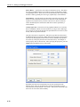
You can now set up defaults for the Setup Screen’s Schedule, Data Files,
Clock, and File Retrieval tabs that will be used when new stations are added to
the network. There is also the ability to copy these defaults to existing stations.
The ability to use 24:00 (rather than the default of 00:00) for the timestamp at
midnight has been added. (This is accessed from the
button next to the
Output Format field on the datalogger’s Data Files tab in the Setup Screen. It is
also available in the Connect Screen’s Custom Collection options.)
PakBus Encryption is now supported for communication between LoggerNet
and CR1000, CR3000, and CR800 series dataloggers. Note that the datalogger
must be running OS 26 or later in order for PakBus Encryption to be used. A
PakBus Encryption Key must be entered in both the datalogger’s device
settings and LoggerNet’s Setup Screen. AES-128 encryption is used.
Two new root devices, SerialPortPool and TerminalServerPool, have been
added to allow for modem pooling (Pooled Devices may be useful in cases
where LoggerNet is used to call, by phone, multiple remote dataloggers and
there is more than one modem and phone line available to make the
connections.)
You can now access a datalogger’s Settings Editor from the Connect Screen
either by right-clicking on the datalogger or from the Datalogger menu. You
can also manually set the datalogger’s clock from the Connect Screen either by
double-clicking in the Station Date/Time field or from the Datalogger menu.
Boolean values displayed in the Connect Screen’s Numeric Display now have
an LED icon next to them to allow for easy toggle.
You can now view additional statistics in the Status Monitor for table-based
dataloggers including watchdog errors, skipped scans, and battery errors. (Note
that there is a Poll for Statistics check box on the datalogger’s Schedule tab in
the Setup Screen that must be enabled to poll for these statistics.)
The Task Master has been integrated into the LoggerNet server. This allows for
remote administration of the Task Master. (See Section 9.1.3, Remote
Administration of the Task Master (p. 9-16), for conditions that must be met for
remote administration of the Task Master.)
NOTE
Integrating the Task Master into the server involved extensive
changes. When upgrading to LoggerNet 4.2 from a previous
version, an attempt will be made to import all previouslyconfigured tasks. However, imports have only been tested back to
LoggerNet 3.4.1. After upgrading (from any previous version of
LoggerNet), you should verify that all of your tasks have imported
correctly.
Calendar-based scheduling has been added to the Task Master. This allows for
non-interval task execution (including data collection). See Example #3 in
Section 9.1.1.4, Define What the Task Does (p. 9-9), for an example of calendarbased data collection.
xvii
Preface — What’s New in LoggerNet 4?
A Constant Customization feature has been added to the CRBasic Editor. This
allows you to define values for one or more constants in a program prior to
performing a conditional compile. The constants can be set up with an edit box,
a spin box field for selecting/entering a value, or with a list box. A step
increase/decrease can be defined for the spin box, as well as maximum and
minimum values.
The CRBasic Editor now allows you to Save and Open Display Settings.
Display settings affect the look and feel of the CRBasic Editor. This includes
font and background, as well as syntax highlighting.
View Pro has a new View Record option in the right-click menu that can be
used to view an entire record in a new window.
The main effort in the development of LoggerNet 4.3 has been support for the
new CR6 Series datalogger. Support was also added for the CRS451 Series
Water Level Recording Sensor and the CRVW Series Vibrating Wire
Recording Interface.
LoggerNet Products
Campbell Scientific offers four LoggerNet software packages, LoggerNet,
LoggerNetData, LoggerNet Admin, and LoggerNet Remote and several
standalone client products. Each of these packages is purchased separately.
LoggerNet is the main software application and comes with all of the
applications needed to set up and configure a network of dataloggers including
tools to write programs and monitor retrieved data. LoggerNetData is a
complementary product that includes applications that can be used on a remote
computer to monitor data, or retrieve, view, and analyze data that was collected
by LoggerNet into a file. LoggerNet Admin and LoggerNet Remote enhance
the capabilities of LoggerNet by providing management tools for more
complex networks. The difference in the two is that LoggerNet Admin offers a
complete LoggerNet package, while LoggerNet Remote, which was designed
to be run remotely, does not include the LoggerNet server.
New and Improved Applications
Several new applications, as well as improvements to previously available
applications, are included with the release of LoggerNet 4.0.
Toolbar
The LoggerNet 4.0 Toolbar has a completely new look and feel. Applications
are divided into categories to make navigating the Toolbar easier. You can also
organize a Favorites category for the applications that you use most often.
Then, if you prefer a smaller version of the toolbar, you can select Favorites
View from the View menu. This will switch to a small view of the toolbar
containing only icons for applications in the Favorites category.
Additional options are available including the ability to show a LoggerNet
system tray icon (either whenever LoggerNet is running or only when
LoggerNet is minimized), the option of hiding the LoggerNet taskbar button
when LoggerNet is minimized and the system tray icon is showing, the option
of whether or not to minimize clients when the Toolbar is minimized, and the
ability to hide or show the main menu.
xviii
Preface — What’s New in LoggerNet 4?
Setup Screen
The Setup Screen now has the option of being used in an EZ View or a
Standard View. The Standard View is similar to the Setup Screen in older
versions of LoggerNet. In the EZ View, the EZ Setup Wizard is used to add
dataloggers and edit their settings.
Standard View Changes
A new menu item has been added to enable a Stations Only view. When this is
enabled, only stations will be shown in the Network Map and they will be
listed in alphabetical order. This can be especially helpful, when working with
a large network.
A Scheduled Backup menu item has also been added. This opens a dialog box
from which you can setup automatic backups of LoggerNet on a user-defined
schedule.
A new root device, the PakBus TcpServer, has been added. This device can
accommodate multiple incoming PakBus/TCP connections to service the
stations attached to it. Therefore, it allows the same IP port to be used to listen
for incoming connections from multiple dataloggers. The device has a Routing
tab that can be used to specify IP addresses and port numbers to be used for
outgoing connections to specific dataloggers attached to the PakBus TcpServer.
The Routing tab can also be used to cause LoggerNet to maintain a connection
with a range of dataloggers, once an incoming connection has been established.
An Image Files tab has been added to the Setup Screen for the CR1000,
CR3000, and CR800 Series dataloggers. This tab provides an easy way to
retrieve image files from the datalogger on a specified interval. (Note this tab
is renamed File Retrieval in LoggerNet 4.1.)
A Notes tab has been added to all devices to allow the user to keep notes about
the device for future reference. This is purely for the user’s convenience. (The
information in a datalogger’s Notes tab is displayed in the Connect Screen,
when that datalogger is selected.)
A new File Output Format option, CSIXML, has been added. When this option
is selected, data is stored in XML format with Campbell Scientific defined
elements and attributes.
Individual devices and/or device branches of the Network Map can be copied
and pasted into the network.
Various other settings have been added including BMP1 Station ID, BMP1
Low Level Delay, PakBus Verify Interval, TCP Password, Enable Automatic
Hole Collection, Stay on Collect Schedule, and Collect At Most. See Section
4.2.4, Device Settings (p. 4-7), or LoggerNet’s online help for information about
these settings and what devices they apply to.
xix
Preface — What’s New in LoggerNet 4?
Connect Screen
The Connect Screen has been reorganized with most of the buttons now
residing on a toolbar at the top of the window.
A Table Monitor has been added in the middle of the window that can be used
to monitor the values for one entire table.
A Notes field has been added that displays the information from the Setup
Screen’s Notes tab of the selected datalogger.
A connection made in the Connect Screen is now subject to the Maximum
Time On-Line configured in the Setup Screen. (See the Device Settings help in
Section 4, Setting up Datalogger Networks (p. 4-1), for information on how the
Maximum Time On-Line setting will affect a connection made using
LoggerNet Admin or LoggerNet Remote 4.0 to connect to a remote server
running an older version of LoggerNet.)
The Pause Data Displays option has been moved to the Edit menu. (In previous
versions it was available as a check box on the Connect Screen.)
The Update Interval for data displays has been moved from the Options dialog
to the display’s main window.
New options added to the data displays include an Auto Format option (rather
than specifying the number of decimal places to display), the ability to format
the timestamp for numeric displays, and the ability to specify what will happen
when a NAN is encountered in a graph.
The configuration of the data displays can now be saved.
A new File Format option, CSIXML, has been added to Custom Collection.
When this option is selected, data is stored in XML format with Campbell
Scientific defined elements and attributes. For Custom Collection, you also
now have the option of whether or not to include timestamps and/or record
numbers.
Status Monitor
Two new statistics are now available to be monitored: Link Time Remaining
(the time remaining, in milliseconds, until Maximum Time On-Line is reached
and the device is automatically disconnected) and RFTD Blacklisted (indicates
that a station has been blacklisted by an RF Base because of a failed
communication attempt).
Task Master
A new event type, After File Closed, has been added to the Task Master. Using
this event type, a task will be executed anytime a data file being written to is
closed.
Along with the above event type, FTP and SFTP capabilities have been added
which allow the just closed file to be transferred to a designated FTP server.
xx
Preface — What’s New in LoggerNet 4?
Short Cut
Support has been added to Short Cut for the CR9000X datalogger, the ET107
Evapotranspiration Monitoring Station, and the AVW200 Two-Channel
Vibrating Wire Spectrum Analyzer.
New sensor files have been added for the CMP3 Pyranometer, the IRR-P
Precision Infrared Temperature Sensor, the JC Ultrasonic Depth Sensor, the
CNR2 Net Radiometer, the CS106 Barometric Pressure Sensor, the OBS-3+
Turbidity Sensor, the 03002 Wind Speed and Direction Sensor, the 105E
(chromel-constantan) Thermocouple, the WindSonic1 (RS-232) TwoDimensional Ultrasonic Wind Sensor, the WindSonic4 (SDI-12) TwoDimensional Ultrasonic Wind Sensor, the HMP155 Temperature and Relative
Humidity Sensor, the SR50A Sonic Ranging Sensor (SDI-12 Output), the
CS450/455 Pressure Transducer, a Vibrating Wire Sensor (for generic
vibrating wire sensors and the AVW200), and a saturation vapor pressure
calculation
An Advanced tab has been added to the Finish screen for CRBasic dataloggers,
which allows the user to view the CRBasic code and launch the CRBasic
Editor.
There is now an option to send the program to the datalogger from the Results
tab on the Finish screen.
The user now has the ability to create custom sensor files using existing sensor
files as templates.
The user can now manually set advanced outputs to high or low resolution.
The Add Device button has been removed. Peripheral devices are now listed in
and selected directly from the Available Sensors and Devices tree.
CRBasic Editor
The CRBasic Editor now gives you the option to Save and Encrypt a file.
Encrypted files can be compiled in the datalogger but cannot be read by a user.
Dim variables can now be declared within a subroutine or function and are
local to that subroutine or function. The same variable name can be used within
other subroutines or functions or as a global variable without conflict. The F9
and F10 pop-up pick list will include the local variables for a specific
subroutine or function if the cursor is within that subroutine or function.
F11 can now be used to bring up a pop-up pick list that contains all userdefined functions found in the program.
A new button has been added to the toolbar (blue arrow) which takes the cursor
to user-defined functions and subroutines.
A new shortcut, CTRL-Y, has been added that will delete the current line.
Several options have been added to the Editor Preferences dialog box
including:
xxi
Preface — What’s New in LoggerNet 4?
Variable Name Matching – When enabled variable names will be
capitalized based on how they are declared in the program, regardless of
how the user may have typed them.
Create .TDF File at Compile – The user can then associate a .TDF file
with a datalogger. This can be useful if communication is taking place
over a slow or unreliable communication link where the attempt to receive
table definitions back from the datalogger fails.
Clear Undo/Redo List on File Save – Clears the change tracking in the
program when the file is saved. Otherwise change tracking is kept until
the file is closed.
Syntax Highlighting for Variables and Local Variables – Variables and
Local Variables can now be given their own syntax highlighting to make
them easier to identify.
You can now drag and drop a file onto the CRBasic Editor workspace to open
the file. Also, multiple files can be selected from the File | Open dialog box.
All selected files will be opened.
Support has been added for custom voice files for the VoiceSpeak instruction.
When inserting a VoiceSpeak instruction, the user then has the option of
choosing words from the standard Voice.txt file or from a user-created custom
voice file.
The CRBasic Editor now has alternate language support, if a separate
LoggerNet language package has been installed.
RTMC
Many new functions have been added that may be used when building
expressions in RTMC. These include string functions, time functions, start
option functions, and function with state. The ability to declare aliases for data
values used in expressions has also been added. See Section 5.2.1.4,
Expressions (p. 5-43), or the Expressions topic in RTMC’s online help for more
information.
RTMC has a new Layout Toolbar which gives quick access to the Align, Space
Evenly, Make Same Size, Center, and Order menu items from RTMC’s
Component menu.
Graphics Options have been added to the Edit | Preferences menu item that
allow you to choose the maximum number of frames per second, whether
animation is enabled, and whether high quality or high speed is more
important. From this menu item, you can also choose the visual theme for
RTMC. This determines the look and feel of the application (i.e. colors, button
appearance, etc.). These options are available in both RTMC Development and
RTMC Run-Time.
An Edit | Customize menu item has been added which allows you to customize
RTMC’s toolbars and menus. This menu item is available in both RTMC
Development and RTMC Run-Time.
Panning functionality has been added to charts in RTMC Run-Time.
xxii
Preface — What’s New in LoggerNet 4?
In RTMC Run-Time, all alarms on a screen can be acknowledged by rightclicking on the screen and then choosing “Acknowledge All On-Screen
Alarms”.
Miscellaneous other changes have been made to the settings for specific
components.
View Pro
View Pro is included for the first time in LoggerNet 4.0. It maintains the ease
of use of our former data file viewer with greatly enhanced capabilities.
Large files can be loaded more quickly. Scrolling is more responsive for large
files.
View Pro allows you to have multiple data files opened at one time. Multiple
graphs can be created from the same file or from multiple files. There is no
limit to the number of traces per graph. Data can be graphed in a variety of
formats including a Line Graph, X-Y Plot, Histogram, Rainflow Histogram, or
FFT (2D or 3D).
You have the ability to create a Line Graph containing multiple strip charts.
This allows you to simultaneously display data from multiple files (one strip
chart per file) to compare data from multiple stations. The X-axes (timestamps)
of the strip charts can be synchronized to facilitate cross file comparisons.
A Line Graph can use record numbers rather than timestamps on the X-Axis.
This allows you to display data files containing gaps in the timestamps.
From the toolbar of a Line Graph, you can bring up a Statistics box which
shows the average, standard deviation, minimum, and maximum of the
displayed points. From the toolbar you can also add a graph cursor to a Line
Graph. The cursor can be scrolled across the graph and the data values and
timestamp at the current cursor position will be shown.
View Pro has zoom capability to allow you to zoom in on a certain area of a
graph. You can also scroll a graph either from the graph itself or from the
opened data file.
You can print a graph either from a preview screen or directly from the graph
toolbar. The graph can also be saved in a variety of formats (BMP, JPEG,
WMF, EMF, or PCX).
Binary files (TOB1, TOB2, TOB3) can be opened directly in View Pro.
Split
A Time Offset option has been added. This allows the user to specify a time
offset that will be applied to each item on the Select line that uses the Date or
Edate function to output a date. This may be useful when adjusting for different
time zones.
Split now maintains a log file, splitr.log, each time Splitr is run. The main
purpose of this log file is to enable users running Splitr in command line mode
to identify what happened with each execution of Splitr. If a second instance of
xxiii
Preface — What’s New in LoggerNet 4?
Splitr is started when one is already running, another log file, splitrunning.log,
will be written. This file simply identifies the time that the second instance of
Splitr was started and that Splitr was already running.
CardConvert
A new File Format option, CSIXML, has been added to the Destination File
Options. When this option is selected, data is stored in XML format with
Campbell Scientific defined elements and attributes.
Troubleshooter
The Troubleshooter now allows the user to customize the possible problems for
which warnings will be given. In addition, you can click on any highlighted
warning to bring up additional information about the warning.
For array-based dataloggers, you now have the option to do a full hardware
reset. You can also now bring up Station Status information for array-based
dataloggers. (Previously this was only available for table-based dataloggers.)
Capability has been added to the Comm Test to report Invalid Datalogger
Security and Invalid LoggerNet Security.
Network Planner
The Network Planner, a graphical application that assists the user in designing
PakBus datalogger networks, is introduced for the first time in LoggerNet 4.0.
The Network Planner allows the development of a model of the PakBus
network, proposes and verifies valid connections between devices, and allows
integration of the model directly into LoggerNet 4.0.
Data Filer
A new File Format option, CSIXML, has been added. When this option is
selected, data is stored in XML format with Campbell Scientific defined
elements and attributes.
You now have the option of whether or not to include timestamps and/or
record numbers in the data file.
RWIS Administrator
RWIS Administrator is a new application that has been added to LoggerNet
which provides support for communication with RWIS (Road Weather
Information Systems) weather stations.
Alternate Language Support
Certain LoggerNet clients can display the user interface component text (for
buttons, dialog boxes, etc.) in a language other than English if a separate
LoggerNet language package has been installed. If a language package is
installed on your machine, you will see the language in the list for the
Languages menu (Options | Languages).
In LoggerNet 4.0, additional applications now have alternate language support.
The applications that now support alternate languages are Setup, Connect,
xxiv
Preface — What’s New in LoggerNet 4?
Status Monitor, Task Master, Short Cut, CRBasic Editor, View Pro, Card
Convert, TroubleShooter, Network Planner, PakBus Graph, LogTool, the
Device Configuration Utility, Data Export, and the RWIS Administrator.
NOTE
Available alternate language packages are provided by Campbell
Scientific’s international representatives or on the CSI website.
They are not included in a standard LoggerNet installation.
xxv
Preface — What’s New in LoggerNet 4?
xxvi
Section 1. System Requirements
1.1 Hardware and Software
LoggerNet is a collection of 32-bit programs designed to run on Intel-based
computers running Microsoft Windows operating systems. The recommended
minimum computer configuration for running LoggerNet is Windows XP,
Windows Vista, Windows 7, or Windows 8 because they offer the most stable
operating environment. LoggerNet runs on both 32-bit and 64-bit versions of
these operating systems.
NOTE
PROTECT YOUR INVESTMENT. Make a back-up copy of your
LoggerNet software and record your CD key. Campbell Scientific
does not replace lost or damaged software. The CD key will be
required for any future installation of the software.
1.2 TCP/IP Service
TCP/IP service must be installed and enabled on the computer for LoggerNet
to run. Contact your IT department for help with enabling TCP/IP service.
1-1
Section 1. System Requirements
1-2
Section 2. Installation, Operation and
Backup Procedures
2.1 CD-ROM Installation
Place the installation disk in your computer’s CD-ROM drive. If autorun is
enabled for the drive, the LoggerNet installation will start automatically. If the
installation does not start automatically, select Start | Run from the Windows’
Start menu. Type D:\Setup.exe (assuming D is your CD-ROM drive letter) in
the Open field. Alternately, use the Browse button to access the CD-ROM
drive and select the Setup.exe file from the disk.
The first screen displayed by the installation is a Welcome screen. Click Next
to proceed to the licensing agreement. After reading the licensing agreement,
select the “I Accept…” option and select Next to proceed to the User
Information screen. At the bottom of the User Information screen is a field for
entering the CD key for the software. The CD key is found on the back of the
CD case in which LoggerNet is shipped. Use the drop-down list box for the
first part of the CD key to select the software being installed: LGRNET
(LoggerNet), LGNADM (LoggerNet Admin), or LGNRMT (LoggerNet
Remote). Note that you must select the correct LoggerNet version for your CD
key or you cannot proceed further in the installation. After entering the CD
key, select Next and continue through the remaining screens, following the onscreen prompts to complete the installation.
Items are added to your computer’s Start menu under Programs | Campbell
Scientific | LoggerNet that start the Toolbar and some other selected utilities.
At the end of installation you also have the option to add a desktop shortcut to
LoggerNet.
By default, the installation copies the LoggerNet program files to the
C:\Program Files\CampbellSci\LoggerNet directory. Many operating system
configurations will require the user name under which the software is installed
to have administrative privileges to the computer. After the software is
installed, administrative privileges are not required by the user to run the
software.
In addition to placing files in the Program Files directory of your computer, the
installation also creates working directories for the LoggerNet server and the
individual LoggerNet applications under C:\CampbellSci. Section 2.3.1,
LoggerNet Directory Structure and File Descriptions (p. 2-2), provides more
detail on the directories that are created.
If you are installing the trial version of LoggerNet, you will have 30 days to
use this fully functional trial version. Each time you run LoggerNet, you will
be advised as to how many days are remaining on your trial version. At the end
of the 30 days, the trial version of LoggerNet will no longer function.
If you choose to purchase LoggerNet, you will need to uninstall the trial
version, run the install program on the LoggerNet CD, and input the CD Key
from the back of your CD case. This can be done either before or after the 30day trial period has expired.
2-1
Section 2. Installation, Operation and Backup Procedures
Note that the trial version will install applications in the C:\Program
Files\Campbellsci\Demo directory. When the purchased version of LoggerNet
is installed, the applications will each be installed in their own directory under
C:\Program Files\Campbellsci.
2.2 Upgrade Notes
If you have any version of LoggerNet 3 installed on your computer, when you
run the installation the existing version will be updated with the new files. If
you have any version of LoggerNet 2 installed, you can choose to upgrade that
installation, or install LoggerNet 4.x separately while leaving the previous
version intact.
When you upgrade an existing installation, LoggerNet will continue to use the
network map, data collection schedules, data file locations, etc., of the existing
installation. Essentially, you will be able to “pick up where you left off” the
last time you used LoggerNet.
LoggerNet 4.x can readily use the network map from LoggerNet 2.x or 3.x.
However, network maps are not backwards compatible. If you upgrade your
existing version, once LoggerNet 4.x is opened, the network map will no
longer be compatible with LoggerNet 2.x or 3.x. For this reason the upgrade
installation will automatically make a copy of the
<WorkingDirectory>\LoggerNet\sys directory and all of its contents. The copy
will reside in <WorkingDirectory>\LoggerNet\
NetworkMapBackup\<version>\sys. If it then becomes necessary to revert
back to a previous version of LoggerNet, you will need to remove the
<WorkingDirectory>\LoggerNet\sys directory and replace it with the
<WorkingDirectory>\LoggerNet\NetworkMapBackup\<version>\sys directory.
If it does become necessary to revert back to an older version of LoggerNet,
you must first uninstall LoggerNet 4.x and follow all prompts given while
uninstalling, including rebooting your computer. You can then install the
previous version of LoggerNet. Note that you cannot expect a backup made in
LoggerNet 4.x to restore properly in an older version of LoggerNet. Also, as
noted above, network maps are not backwards compatible. Trying to use a 4.x
network map in an older version of LoggerNet may corrupt the network map
such that it can no longer be used in LoggerNet 4.x.
2.3 LoggerNet Operations and Backup Procedures
This section describes some of the concepts and procedures recommended for
routine operation and security of the LoggerNet software. If software and
computer systems were perfect this section would not be necessary. However,
since this software is required to run with predictable results in the real world
on real computers, the following guidelines and procedures will be helpful in
minimizing possible problems that may occur.
2.3.1 LoggerNet Directory Structure and File Descriptions
2.3.1.1 Program Directory
As described in the installation procedures, all of the files for program
execution are stored in the C:\Program Files\Campbellsci\LoggerNet directory.
This includes the executables, DLLs, and most of the application help files.
2-2
Section 2. Installation, Operation and Backup Procedures
This directory does not need to be included in back up efforts. LoggerNet and
its applications rely on registry entries to run correctly; therefore, any
restoration of the program should be done by reinstalling the software from the
original CD.
2.3.1.2 Working Directories
In this version of LoggerNet, each major application keeps its own working
directory. The working directory holds the user files created by the
application, as well as configuration and initialization (*.INI) files. Because of
this working directory scheme (implemented in version 3.0), when you use File
| Open in Edlog, CRBasic Editor, Split, etc., you may find yourself in an
unfamiliar directory and may have to navigate to a different directory to find
existing data files, datalogger programs, etc.
This scheme was implemented because we use the underlying tools and many
of the applications (the server itself, library files, datalogger program editors,
etc.) in a number of different products. By providing a common working
directory for each major application, we hope to make it easier to keep track of
files and information as you move from one product to another.
The following figure shows the typical working directories for LoggerNet if
the default options were selected during installation.
2-3
Section 2. Installation, Operation and Backup Procedures
By default, the files that you create in each of the applications will be stored in
their respective folders in the working directory. You can override that default
and store the files in a different location. Each application “remembers” the
last directory in which a file was saved and will default to that directory until a
different directory is selected.
Note that most all applications have one or more subdirectories in which
configuration files are saved.
Lib directory – The Lib directory is a library directory for several of the
LoggerNet applications. The Compilers folder holds all of the compilers for
the CRBasic Editor, except for the CR200 compilers, which are stored in the
CR200Compilers directory. The CRBasicDefFiles folder holds the definition
2-4
Section 2. Installation, Operation and Backup Procedures
files and help files for all dataloggers supported by the CRBasic Editor. The
definition files are the files which provide the unique instructions and
parameters for each datalogger. The RTMCMediaLib directory contains all of
the media files that can be used by RTMC to provide graphics and sound for
your RTMC projects. Any custom graphics or sounds that you create and wish
to use in your project should be stored in one of these directories.
DevConfig and DevConfigLib directories – These directories contain the
files for each datalogger that will be used by the Device Configuration Utility.
LoggerNet directory – The ASCII data files that are saved to disk as a result
of data collection from the dataloggers are stored to the LoggerNet directory
with a *.dat extension. The Logs directory holds the logs that are created when
communication takes place between the LoggerNet server and client
applications, and the LoggerNet server and the dataloggers. These logs are
used to help troubleshoot communication problems.
The Sys directory holds the network map description (CsiLgrNet.xml) and the
binary data cache. (The data cache is a repository for the data which is
collected from the dataloggers by the LoggerNet server, and which each client
application accesses when processing that data. In the example above, folders
20, 28, and 33 represent the data caches for different dataloggers. See
Appendix D, Software Organization (p. D-1), for additional information.)
2.3.2 Backing up the Network Map and Data Files
As with any computer system that contains important information, the data
stored in the LoggerNet working directory should be backed up to a secure
archive on a regular basis. This is a prudent measure in case the hard disk
crashes or the computer suffers some other hardware failure that prevents
access to the stored data on the disk.
The maximum interval for backing up data files depends primarily on the
amount of data maintained in the datalogger memory. The datalogger’s final
storage is configured as ring memory that will overwrite itself once the storage
area or table is full. If the data is backed up more often than the oldest records
in the datalogger are overwritten, a complete data record can still be maintained
by restoring the data from the backup and then re-collecting the newest records
from the datalogger.
2.3.2.1 Performing a Manual Backup
LoggerNet provides a simple way to back up the network map, the LoggerNet
data cache, and user created files such as program files (CSI, DLD, or CR*),
Split report files (PAR), or ASCII data files (DAT). From the Setup Screen’s
menu, choose Backup | Manual Backup. This opens the Backup wizard that
steps you through the process of creating the backup file.
You can choose to back up only the network map, or to back up the network
map and data cache. The network map will restore all settings and data
collection pointers for the dataloggers and other devices in the network. The
data cache is the binary database which contains the collected data from the
datalogger. Other files can be added as well.
2-5
Section 2. Installation, Operation and Backup Procedures
The backup file is named LoggerNet.bkp and is stored in the
C:\CampbellSci\LoggerNet directory (if you installed LoggerNet using the
default directory structure). You can, however, provide a different file name if
desired.
2.3.2.2 Performing Scheduled Backups
LoggerNet also provides a simple way of backing up your network on a
specified interval. From the Setup Screen’s menu, choose Backup | Scheduled
Backup. When this menu item is chosen, the subsequent dialog box allows you
to specify the backup base date and time, the backup interval, any files to be
backed up in addition to the network map, whether the backup includes the
LoggerNet cache, the name of the backup file, and the number of backup files
that will be kept before the oldest is overwritten
2.3.2.3 Performing Backups from the Task Master
A backup can be performed automatically by setting up a task in LoggerNet’s
Task Master. This can be useful to perform a backup every time a certain
event type occurs. It may also be used to perform a scheduled backup, but that
function is performed more easily from the Setup Screen’s Scheduled Backup
function as described above.
The files included in the backup will be based on a saved backup configuration
file. To save a backup configuration, choose Backup | Manual Backup from the
Setup Screen’s menu. Proceed through the Backup wizard. At the last step,
choose Save Configuration For Later. The configuration will be saved to
C:\Campbellsci\LoggerNet\Backup.Configuration.
To set up the task, open the Task Master and add a task. For an “Add After”
task, choose the event type that will trigger the backup. For a scheduled task,
enter the interval on which you want the backup to be performed. Press the
Configure Task button and enable the Execute File check box. In the File
Name field, type (or browse for) the file LNBackup.exe. Make sure to include
the path (if LoggerNet was installed with the default directory structure, this
will be C:\Program Files\CampbellSci\LoggerNet\LNBackup.exe). Once the
changes have been applied, the backup will be performed based on the defined
event or schedule.
To create a unique filename based on date and time each time the task is run,
enter –AppendTime in the Command Line options field.
If you are running LoggerNet Admin and have security enabled, the command
line options must also include the username and password as shown below:
-username=“username” –password=“password”
If you have used a LoggerNet command line argument (see Section 3.2.1.4,
Command Line Arguments (p. 3-4)) to change LoggerNet’s default port number,
the command line options must also include the server address and port number
as shown below:
-server=server_address:port (e.g. LocalHost:6700 or 192.168.7.123:6700)
2-6
Section 2. Installation, Operation and Backup Procedures
Automatic Backup Configured in Task Master
2.3.2.4 Restoring the Network from a Backup File
To restore a network from a backup file, choose Backup | Restore Network.
Select the *.bkp file that contains the network configuration you want to
restore. Note that this process DOES NOT append to the existing network —
the existing network will be overwritten when the restore is performed.
2.3.3 Loss of Computer Power
The LoggerNet communications server writes to several files in the \SYS
directory during normal operations. The most critical files are the data cache
table files and the network configuration files. The data cache files contain all
of the data that has been collected from the dataloggers by the LoggerNet
server. These files are kept open (or active) as long as data is being stored to
the file.
The configuration files contain information about each device in the datalogger
network, including collection schedules, device settings, and other parameters.
These files are written to frequently to make sure that they reflect the current
state and configuration of each device. The configuration files are only opened
as needed.
2-7
Section 2. Installation, Operation and Backup Procedures
If computer system power is lost while the LoggerNet server is writing data to
the active files, the files can become corrupted, making the files inaccessible to
the server.
While loss of power won’t always cause a file problem, having files backed up
as described above will allow you to recover if a problem occurs. If a file does
get corrupted, all of the server’s working files need to be restored from backup
to maintain the synchronization in the server state.
2.3.4 Program Crashes
If the communication server crashes, there is a possibility that files can be
corrupted (note, however, that corruption is much less likely with a program
crash than during a power loss, since the computer operating system remains in
control and can close the files left open by the failed program). If, after a
program crash, the server does not run properly, you may need to restore the
data from backup.
If you have problems restarting the LoggerNet server after a program crash or
it crashes as soon as it starts, make sure that the LoggerNet server has not left a
process running. You can check this by going to the Windows Task Manager
and selecting the Process tab. In the list of processes look for the Toolbar or
one of the client applications. If one of these processes exists but the Toolbar
is not running, select this process and click “End Process”; you will be asked to
confirm the end process.
2.4 Installing/Running LoggerNet as a Service
If you have LoggerNet Admin, you can install and run LoggerNet as a service.
The advantage of running a software application as a service is that the
software will run even when no user is logged in to the computer system. Some
users may desire to run LoggerNet as a service, so that in the event of a loss of
computer system power LoggerNet will resume data collection and scheduled
task activities when power is restored to the computer and it “boots up”.
LoggerNet Admin includes LoggerNet Service Manager, which is used to
install and control LoggerNet when running as a service. The LoggerNet
Service Manager is opened from the Windows Start menu (Start | Programs |
Campbell Scientific | LoggerNet | LoggerNet Service Manager). The
LoggerNet Service Status box at the top of the LoggerNet Service Manager
window indicates whether or not LoggerNet is installed as a service and
whether or not the service is running. When you first open the LoggerNet
Service Manager, if LoggerNet has not been installed as a service you will
need to select the Install button. Note that LoggerNet must be closed to install
it as a service. If it is opened, you will be prompted to close it before you can
continue.
Once LoggerNet is installed as a service, you can use LoggerNet Service
Manager to Start the service (or Stop it if it is enabled). The LoggerNet service
can be uninstalled by selecting the Uninstall button.
One caveat to running LoggerNet as a service is if LoggerNet uses system
resources (such as a COM port that is continuously open waiting for datalogger
call-back attempts) these resources will be unavailable to other applications
until the service is stopped.
2-8
Section 2. Installation, Operation and Backup Procedures
Note that when running LoggerNet as a service, tasks being run by the Task
Master cannot interact with the desktop. Therefore, any tasks set up in the
Task Master should not require any user interaction.
If LoggerNet is installed as a service, the service must be running for
LoggerNet to run (either automatically or manually). You will be prompted to
start the service if you try to launch LoggerNet manually when the service is
installed but not running.
The first time LoggerNet is installed as a service, a LoggerNet user account is
created. The LoggerNet service is run under this LoggerNet user account. This
allows the LoggerNet Service to always run in the same environment with
known user rights. You will be asked to enter and confirm a password for the
LoggerNet user account. The password you enter can later be used to log in to
the computer as the LoggerNet user. The password can be changed by pressing
the Options button and then pressing Change Password.
NOTE
If the machine has a preexisting LoggerNet user account created
from LoggerNet 3.4, it will be necessary to stop, uninstall the
service, then reinstall the service in order to setup the password.
NOTE
The LoggerNet user account will not show up in your list of users
when logging on to your computer. It can be viewed from the
Windows Control Panel. (In Windows 7, for example, from the
Control Panel, click User Accounts | Manage User Accounts |
Advanced tab | Advanced button, and then select Users from the
list of Local Users and Groups.) Although it is not available in the
drop-down list when logging on to your computer, you can
manually enter the user name (LoggerNet), enter the password,
and then select your local machine. (In Windows 7, the local
machine name is entered with the user name, i.e.,
machine_name\LoggerNet.)
2.4.1 Issues with Running LoggerNet as a Service
By default, the LoggerNet service is run under the LoggerNet user account.
This may cause some issues with write access and network drives. The issues,
along with their solutions, are described below:
2.4.1.1 Write Access
The LoggerNet user has write access only to the CampbellSci directories.
Therefore, if a task requires something to be written or done in a different
directory or on the desktop, the LoggerNet user does not have sufficient access
and the process will end in an error. This can be solved by giving the
LoggerNet user write access to the necessary directories.
2-9
Section 2. Installation, Operation and Backup Procedures
Giving the LoggerNet user write access
This is the process for giving the LoggerNet user write access to a designated
directory in Windows XP. The process in other operating systems is similar.
•
Right-click on the directory in Windows Explorer and choose
Properties.
•
Go to the Security tab of the Properties dialog box and select Add. This
will open the Select Users, Computers, or Groups dialog box.
•
From the Select Users, Computers, or Groups dialog box press the
Locations button. This will open the Locations dialog box.
•
In the Locations dialog box, select the computer name and press OK.
•
From the Select Users, Computers, or Groups dialog box press the
Advanced button. Then press the Find Now button. Select LoggerNet in
the list of names that appears at the bottom of the dialog box and press
OK. Note that <COMPUTER-NAME>/LoggerNet has been added to the
Object Names on the Select Users, Computers, or Groups dialog box.
Press the OK button to close the Select Users, Computers, or Groups
dialog box.
•
The LoggerNet user should now be highlighted on the Properties dialog
box. Select the Full Control Allow check box to give LoggerNet full
permissions for the directory. Press the Apply button to apply the changes.
Press OK to close the dialog box.
•
The LoggerNet user should now have full access to the designated
directory.
2.4.1.2 Network Drives
Network drive mappings are associated with individual user accounts.
Therefore, they cannot be used when running LoggerNet as a service. To use
network drives when running LoggerNet as a service, you must use the full
UNC path (e.g., \\computer_name\directory\filename). Note that the ability to
write to the network drives will be governed by Windows security. It will be
necessary to configure the LoggerNet service to run under an account that has
network privileges. This requires changes to the properties of the LoggerNet
service in Windows. Contact your network administrator for assistance.
2.5 Special Note on Windows XP Service Pack 2
With Service Pack 2, Microsoft has automatically enabled a firewall
application on each individual PC. This was done to protect PCs from invasion
by outside, unauthorized programs that may try to connect via a socket using
TCP/IP.
Remember, however, that LoggerNet is a client-server application that uses
TCP/IP as the link between clients and the server. This means that windows
such as Setup, Connect, Status Monitor, RTMC, etc., get their access to devices
and data only through the LoggerNet server. While, in the basic LoggerNet
installation most of these clients typically access the server on the same PC
2-10
Section 2. Installation, Operation and Backup Procedures
(which will already be “behind” the PC’s local firewall), the server is capable
of distributing the same information to similar clients connected via TCP/IP
from anywhere in the world, revealing the true power of the client-server
design. If, for example, you want others to use RTMC or Data Filer to get data
from your LoggerNet PC, you can enable this remote connection by selecting
the Allow Remote Connections check box on the dialog box opened from
LoggerNet’s Tools | Options menu item. This causes the server to open a
socket on a specific port (default is port 6789) to listen for requests for data
from its clients. This is usually quite safe since: 1) no other application should
be trying to use this port, and 2) the server will only respond to LoggerNetspecific messages on this port (it will not run viruses or other unauthorized bits
of code). If you allow remote connections, however, the firewall in Windows
XP SP2 will put up a window telling you that it has blocked “Toolbar” and
asking if you wish to unblock Toolbar from Campbell Scientific. At this point,
if you click “Unblock”, Windows XP will make an exception for LoggerNet
and you should not have to unblock it each time you start it. You can reverse
this decision by opening the Windows Control Panel, selecting Windows
Firewall, and deleting Toolbar from the list of exceptions.
2-11
Section 2. Installation, Operation and Backup Procedures
2-12
Section 3. Introduction
3.1 What is LoggerNet?
LoggerNet is a software application that enables users to set up, configure, and
retrieve data from a network of Campbell Scientific dataloggers and share this
data over an Ethernet communications network. This software application is
designed to run under Windows XP, Windows Vista, and Windows 7.
LoggerNet software supports communication and data collection for Edlog
dataloggers including the CR500, CR510, CR10, CR10X, 21X, CR23X, and
CR7 in any of their mixed-array, table data, or PakBus operating systems, and
the CRBasic dataloggers including the CR200 Series, CR1000, CR3000,
CR800 Series, CR6 Series, CR5000, CR9000, and CR9000X.
The LoggerNet software is written using advanced “client-server” architecture.
The server software engine runs in the background handling all of the
datalogger communications. The server also takes care of storing the data and
providing information to manage the datalogger network. In turn, the client
applications connect to the server to access the information collected from the
dataloggers.
One significant benefit of the software design is that some of the client
applications (RTMC, for instance) can be run on any computer that connects to
the main computer by a TCP/IP network connection. Some examples of these
networks are Local Area Network (LAN), Wide Area Network (WAN), or the
Internet. If you have LoggerNet Admin or LoggerNet Remote, any of the
client applications can log on to a remote LoggerNet server. Another benefit is
the efficiency that is gained, since several client applications can
simultaneously request and receive information from the software server.
LoggerNet is an ideal solution for users wanting a reliable data collection
system that is also flexible enough to meet a variety of needs.
3.1.1 What Next?
The ultimate goal with most datalogging applications is to retrieve data to a
computer for further analysis and manipulation. Now that you have installed
LoggerNet on your computer, how do you reach that goal?
The first step is to set up a communication link between your computer and the
datalogger station. This step may also include the configuration of peripheral
communication devices. Next you’ll need to develop a program for the
datalogger, and then send the program to the datalogger and ensure that
measurement results are viable. Once the datalogger has been storing data for
a period of time, you will want to collect that data and store it to a file on your
computer for further analysis.
LoggerNet provides the tools to accomplish these steps, as well as tools to
resolve problems along the way if they should arise. The remainder of this
section briefly reviews the steps and the various tools that can be used to
accomplish them. More detailed information is provided in the subsequent
sections of this manual.
3-1
Section 3. Introduction
3.2 Overview of Major LoggerNet Functions and
Associated Software Applications
3.2.1 The Heart of it All – LoggerNet Toolbar
The LoggerNet Toolbar has several functions. The most important is starting
the server that handles all communications with the dataloggers in the network.
As long as the Toolbar is running, either visible or minimized, the server is
working and able to communicate with the dataloggers. Shutting down the
Toolbar also shuts down the server and suspends all communications with the
dataloggers in the network.
When you run LoggerNet from the Window’s Program menu or from a desktop
shortcut, you are launching the LoggerNet Toolbar. Some options on the
Toolbar launch applications that connect to the server and allow you to set up
the network or view the collected data. Other options launch stand-alone
applications to perform other functions, such as program editing. As you hover
over a category in the list on the left side of the toolbar, applications related to
that category will be shown on the right. Selecting an application in the righthand list will launch the application.
LoggerNet’s client-server design allows client applications to be run on the
same computer as LoggerNet, or on remote computers running LoggerNetData,
LoggerNet Admin, or LoggerNet Remote. Note that the LoggerNet Toolbar
must be up and running (or LoggerNet must be running as a service) and
Remote Connections must be enabled for remote computers to access a
LoggerNet server. For additional information on Remote Connections, refer to
Section 12.1, Allowing Remote Connections to the LoggerNet Server (p. 12-1).
3.2.1.1 Toolbar Views
When first opened, LoggerNet displays a full view of the Toolbar.
If you prefer a smaller version of the toolbar, you can select Favorites View
from the View menu. This will switch to a small view of the toolbar containing
only icons for applications in the Favorites category. (For additional
information on the Favorites category, refer to the following section.)
3-2
Section 3. Introduction
By default, the LoggerNet menus are not shown on the toolbar. Press the arrow
button in the upper right corner to view the LoggerNet menus as shown below.
The arrow button will change direction and can then be used to hide the menus.
3.2.1.2 Favorites Category
The Favorites category can be configured to display as many or as few
applications as desired by selecting the Tools | Options menu item and then
using the Favorites tab.
The Available Applications column shows all applications that are available in
LoggerNet. (Press the + sign next to a category to show the applications in that
category.) An application can be added to the Favorites category by selecting it
in the Available Applications column and pressing the right arrow key. An
application can be removed from the Favorites category by selecting it in the
Favorites column and pressing the left arrow key.
The applications will appear on the Toolbar’s Favorites category in the same
order as they appear in the Favorites column. The up and down arrow keys can
be used to rearrange the order of applications in the Favorites column. To move
3-3
Section 3. Introduction
an application up in the Favorites column, select the application and press the
up arrow until the application is in the desired location. Use the down arrow
key in a similar manner to move the application down in the Favorites column.
3.2.1.3 Toolbar Menus
The following options are available from LoggerNet’s menu:
File Menu
Exit – Closes the LoggerNet application.
View Menu
Full View – This option is only available when in Favorites View and brings
up the full view of the Toolbar.
Favorites View – This option is only available when in Full View. It switches
from a full view of the Toolbar to a smaller view which shows icons for only
the Favorites category.
Hide Main Menu – Hides LoggerNet’s main menu. The main menu can be
displayed again by pressing the arrow key in the upper right-hand corner of the
Toolbar.
Tools Menu
Options – This option bring up the LoggerNet Options dialog box. From this
dialog box you can specify various options such as whether the toolbar always
stays on top, the behavior of the system tray icon, language, whether remote
connections are allowed, and whether IPv6 connections are allowed. You are
also able to specify which applications are included in the Favorites category.
Launch Menu
Provides a drop-down list of all the categories on the LoggerNet toolbar.
Hovering over a category will display a list of applications related to that
category. When an application is selected from this list, it will be started.
Help Menu
LoggerNet Help – Opens the LoggerNet on-line help file.
Check for Updates – Opens Campbell Scientific’s website to check for updates
to LoggerNet.
Give Feedback on LoggerNet – Opens a form on our website which allows you
to provide feedback on LoggerNet to Campbell Scientific.
About LoggerNet – Displays version and copyright information for LoggerNet.
3.2.1.4 Command Line Arguments
Command line arguments allow you to change LoggerNet’s default behavior
when it is started from a shortcut.
3-4
Section 3. Introduction
Currently, there are three command line arguments:
/WorkDir Sets the working directory to something other than the default.
Usage:
“C:\Program Files\CampbellSci\LoggerNet\ToolBar.exe”
/WorkDir=C:\CampbellSci\test
where “C:\Program Files\CampbellSci\LoggerNet\ToolBar.exe”
is the directory and filename for the LoggerNet Toolbar (which
essentially is the LoggerNet server) and C:\CampbellSci\test is the
working directory to be used.
/M
Launches LoggerNet in a minimized state. Usage:
“C:\Program Files\CampbellSci\LoggerNet\ToolBar.exe” /m
/IPPORT=XXXXX Causes the server to use port XXXXX for TCP/IP
communications with clients. Handy if some other software is
using the default port of 6789. Usage:
“C:\Program Files\CampbellSci\LoggerNet\ToolBar.exe” /ipport=12345
NOTE
If you are running LoggerNet Admin, which requires that you log
in to a particular sever with each client, you must specify this
alternate port number when entering the server address in the login
window (e.g., LocalHost:6700 or 192.168.7.123:6700).
NOTE
If LoggerNet is being run as a service (available in LoggerNet
Admin), you use LoggerNet Service Manager to specify an
alternate working directory or IP port.
3.2.1.5 Alternate Language Support
Certain LoggerNet clients can display the user interface component text (for
buttons, dialog boxes, etc.) in a language other than English if a separate
LoggerNet language package has been installed. If a language package is
installed on your machine, you will see the language in the list at Tools |
Options | Languages. When a new language is chosen, the Toolbar will
immediately reflect the change. Opened clients will not reflect the change until
they are closed and reopened.
Applications that support alternate languages are Setup, Connect, Status
Monitor, Task Master, Short Cut, CRBasic Editor, View Pro, CardConvert,
TroubleShooter, Network Planner, PakBus Graph, LogTool, the Device
Configuration Utility, Data Export, and the RWIS Administrator.
NOTE
Available alternate language packages are provided by Campbell
Scientific’s international representatives or on the CSI website.
They are not included in a standard LoggerNet installation.
3-5
Section 3. Introduction
3.2.2 LoggerNet Admin/LoggerNet Remote
LoggerNet Admin and LoggerNet Remote add functionality to aid in the
management of networks. One of these additions is the ability to access a
LoggerNet server from a remote computer. To do this, you need to “log in” to
the remote server. All of the standard LoggerNet clients that are capable of
accessing remote servers (such as Setup, Connect, or Status) include a Select
Server dialog box under the application’s File menu. This allows the user to
specify the TCP/IP address, as well as a user name and password if security is
enabled, for the remote server.
LoggerNet Admin and LoggerNet Remote also have the ability to launch more
than one of the same client screens. In LoggerNet, you can open only one client
window at a time. In LoggerNet Admin/LoggerNet Remote, if Launch Multiple
Clients is selected on the Toolbar’s Option menu, you can open two or more of
the same window. For instance, you can open one Connect Screen and connect
to datalogger A, and open a second Connect Screen and connect to datalogger
B.
3.2.3 Setting Up Datalogger Communication Networks
Network setup tools allow you to define and configure the dataloggers in the
network, how they are connected to the computer, and what data should be
collected.
The most basic tool in setting up your network is the Setup Screen. The Setup
Screen can be used in either an EZ View or a Standard View. (For simplicity,
in this manual, references to the Setup Screen that do not specify EZ View or
Standard View, will refer to the Standard View of the Setup Screen.)
The EZ View of the Setup Screen uses the EZSetup Wizard which provides a
simple step-by-step sequence of screens, with on-screen help and many pre-set
values that make it easy to add a new datalogger and communications devices
to your LoggerNet network. You start with the type of datalogger you wish to
add, and then enter the settings for the communications devices used to reach
it, ending with a communications test and an opportunity to set the clock, send
a program, and set up an automatic data collection schedule.
The Standard View of the Setup Screen accomplishes the same tasks, but
allows you a bit more control when setting up your network, and allows for
more complex network configurations.
The Device Configuration Utility, or DevConfig, uses a direct serial port or IP
connection to set the settings in a device (such as the PakBus address or routing
information for a datalogger, or RF400 radio information) so that LoggerNet
can communicate with it. It can also be used to send a new operating system to
devices that accept a downloadable OS. DevConfig supports all CSI
dataloggers, as well as configurable communication devices such as RF400
radios, MD485s, and NL100s.
The Network Planner is a graphical application that assists the user in
designing a datalogger network. The user interacts with a drawing canvas on
which he places his stations and adds peripheral devices to those stations. He
then creates links between stations and specifies the nature of those links.
Finally, he specifies the activities that will take place between various devices
within the network. As the user does these things, the Network Planner
3-6
Section 3. Introduction
automatically specifies many individual device settings such as PakBus
address, neighbor lists, verify intervals, network parameters, etc. The Network
Planner also provides an interface to allow the user to actually configure the
dataloggers and peripheral devices in his network as well as the LoggerNet
server.
LoggerNet also ships with a command line scripting tool, CoraScript, which
can be used to configure the datalogger network from a command prompt.
LoggerNet’s Scheduled Backup, Manual Backup, and Restore Network tools
are useful for backing up the entire datalogger network (refer to Section 2.3.2,
Backing up the Network Map and Data Files (p. 2-5)).
3.2.4 Real Time Tools
LoggerNet’s real-time tools are used to connect to a datalogger, set the clock
and send a program to the datalogger, and view the data being collected from
the datalogger by the LoggerNet server. These tools include the Connect
Screen and RTMC.
The Connect Screen is used primarily for initializing or checking operation of a
datalogger and manually collecting data. This screen provides near real-time
communication with a datalogger. Utilities are available for sending programs
to or retrieving programs from a datalogger, checking or setting a datalogger
clock, and getting status information from the datalogger. There are windows
for displaying data either graphically or in numeric format, as well as setting
input locations, ports, and flags. You can also manually retrieve data in
various formats, and communicate with a datalogger in terminal emulation
mode.
RTMC is used to for real-time data displays of the data collected by the
LoggerNet server. You can create customized graphic displays that include
graphs, tables, dials, alarms, digital values and other graphic elements. These
displays automatically update when LoggerNet collects new data. Graphical
elements are also available for toggling ports or flags, or setting variables (or
input locations) in a datalogger. The displays created in RTMC can be
distributed to other users who have licenses to run RTMC Run-time software
(purchased separately). This allows a remote computer, accessible via TCP/IP,
to connect to the LoggerNet server and display the real-time data.
3.2.5 Network Status and Problem Solving
Since communications invariably fail at some point, LoggerNet includes
several tools to pinpoint where the problem lies.
The Status Monitor is used to monitor the health of datalogger network
communications. The integrity of the communications link can be verified
quickly from the color of the status icon for each device. A Communications
History graphic shows the success of communications over the last 24 hours.
Columns can be set up to display detailed statistics on communications quality
and data collection. For troubleshooting purposes, The LogTool application is
available to view operational log messages for the server as well as the lowlevel communication between the datalogger and the server. A Comm Test
window can also be launched from the Status Monitor.
3-7
Section 3. Introduction
Troubleshooter is used to identify possible problems disrupting
communications or data collection. You can narrow the display to show only
the dataloggers in the network, or expand it to view the entire network.
Problems are highlighted in different colors to indicate levels of severity. You
can click on a potential problem to bring up a menu that allows you to go to the
Setup Screen or Status Monitor to fix the problem, bring up help on the
problem, or in some cases fix the problem directly. Finding a problem, you
can launch a separate Communications Test utility or open the server logs.
PakBus Graph provides a graphical display of a PakBus network, and quick
access to the PakBus settings in LoggerNet and other PakBus devices. PakBus
is a packet-switched protocol developed by Campbell Scientific that facilitates
communications between PakBus-capable devices, including dataloggers, some
communications peripherals (NL100s, RF400s, etc.), and LoggerNet itself.
Among the advantages of PakBus are: more robust communications due to
packet-based communications, multi-threading of communications (e.g., you
can use a keyboard/display at the same time as a PC is collecting data via
telecommunications; or two PCs can request data from a datalogger at the same
time), peer-to-peer communications (PakBus dataloggers can send to or request
data from other PakBus dataloggers without a PC involved), and dynamic
routing (PakBus devices can be configured as “routers” and learn about the
presence of other PakBus devices or alternative routes to those devices as they
come on line or routes change).
In addition to these tools, a Troubleshooting guide is provided in this manual.
Refer to Section 14, Troubleshooting Guide (p. 14-1).
3.2.6 Network Management Tools
LoggerNet Admin includes some tools which are useful when managing large
networks, or when you need to manage networks with several users.
The LoggerNet Service Manager is a utility that allows you to install and run
LoggerNet as a service. Refer to Section 2.4, Installing/Running LoggerNet as
a Service (p. 2-8), for additional information.
The Security Manager allows a LoggerNet network administrator to set up
accounts for each user on a system, and then allow each user access rights to
LoggerNet under one of five levels of security. The Security Manager is
available only with LoggerNet Admin or LoggerNet Remote. Refer to Section
11, Utilities Installed with LoggerNet Admin and LoggerNet Remote (p. 11-1), for
details.
The Hole Monitor utility is used to monitor the hole collection activity in
LoggerNet. Holes are instances in the data cache where records are missing.
Holes are most often seen in large RF networks where data is being collected
via a data advise operation.
3.2.7 Creating and Editing Datalogger Programs
LoggerNet offers two programs editors (one for CRBasic datalogger programs
and one for Edlog datalogger programs), and a program generator (which
supports both programming language types).
3-8
Section 3. Introduction
For straightforward “measurement/control/data storage” datalogger programs,
the Short Cut program generator is an excellent choice for datalogger program
creation. Short Cut prompts you for the type of datalogger, scan interval,
sensors to be measured (including those on multiplexers and other peripherals),
and desired final storage output. It then creates the program for you, along
with a wiring diagram showing how each of the sensors should be connected to
the datalogger. Short Cut’s resulting programs can even be imported into
Edlog or CRBasic Editor when you want to get a head start on more elaborate
programs. Short Cut is also available from the Campbell Scientific website
(www.campbellsci.com) so you can update it with newer sensor files as they
become available.
NOTE
While Short Cut programs can be imported into Edlog or the
CRBasic Editor, once they have been edited in one of these
programs, the modified program cannot be imported back into
Short Cut.
The CRBasic Editor is a program editor for the CR200 Series, CR1000,
CR3000, CR800 Series, CR6 Series, CR5000, and CR9000 dataloggers.
Instructions are included for sensor measurement, program and peripheral
control, data storage, and peer-to-peer data transfer. The editor checks for
program validity and offers many user-configurable options to make editing
long programs easier.
Edlog is the tool to create and edit datalogger programs for all Campbell
Scientific dataloggers except the CR200 Series, CR1000, CR3000, CR6 Series,
CR5000, CR800 Series, and CR9000. Instructions are available for sensor
measurement, intermediate processing, program and peripheral control, and
data storage. The built-in precompiler provides error checking and warns of
potential problems in the program. For Edlog dataloggers with PakBus
operating systems, you can include settings for PakBus routing in the
datalogger program itself.
For those users of CR10X or CR510 dataloggers and Edlog programming who
are switching to CR1000 dataloggers (or CR23X users switching to CR3000
dataloggers), a Transformer utility has been developed. The Transformer reads
in an Edlog CSI or DLD file and generates a CRBasic program file. The two
files are displayed side-by-side for comparison purposes; double-click an
instruction in the Edlog program, and the associated instruction is highlighted
in the CRBasic program. Edlog program instructions that cannot be converted
directly to a CRBasic program instruction are listed in a Messages window and
are included as commented text in the CR* file. After conversion, the newly
created CR* file can be opened in the CRBasic Editor for further editing.
3.2.8 Working with Data Files
LoggerNet includes applications that allow you to view and process the data
collected from the dataloggers. These include the file viewer, View Pro, a
report generation tool, Split, and CardConvert (a binary data file file
converter).
View Pro is used to inspect data files, from either mixed-array or table data
dataloggers. You can also view data from an LNDB database. The data is
displayed in a tabular format by record or array. Data values can then be
chosen to display graphically on a line graph, histogram, XY plot, rainflow
3-9
Section 3. Introduction
histogram, or FFT as appropriate for the data type. You can also print graphs
or save them to disk in a variety of formats.
Split is used to post process and generate reports from collected data files from
either mixed-array or table-based dataloggers. Traditionally it has been used to
separate mixed-array data files into individual files based on the array ID, but it
can also create files in custom formats for use in reports or as input to other
data applications, including converting mixed-array datalogger time stamps
(year, Julian day, Hour/Minute) to more conventional date/time stamp formats.
Split includes time series function, which can be used to provide summary
information from more frequent data (e.g., hourly summaries from one-minute
data).
The CardConvert file converter is used to convert TOB1, TOB2, and TOB3
files to TOA5, Array Compatible CSV, or CSIXML format (TOB2/TOB3 files
can also be converted to TOB1 format). TOB files are binary files that are
either created by LoggerNet during collection or are collected directly from a
compact flash, microSD, or PCMCIA card installed in a CRX000 datalogger.
A command line file converter, toA_to_tob1, is also included in LoggerNet.
(Refer to Appendix B, Campbell Scientific File Formats (p. B-1), for additional
information on File Formats.)
3.2.9 Automating Tasks with Task Master
The Task Master is used to set up a Task that can be triggered on a defined
schedule or upon a data collection event from a datalogger. A Task can be data
collection from another datalogger, the transfer of a just collected data file to a
designated FTP directory, or anything that can be executed in a computing
environment (i.e., a command line operation, a program executable, a batch
file, or a script).
3.2.10 Managing External Data Storage Devices
CardConvert is used to retrieve binary data from a compact flash, microSD, or
PCMCIA card, convert it to an ASCII or binary file, and save it to disk.
CardConvert supports binary data generated by CRX000 dataloggers.
The File Control functionality, accessed from the Connect Screen, can be used
to manage files created by CRX000 dataloggers on other, non proprietary
formatted, PC cards.
3.2.11 Optional Client Products Compatible with LoggerNet
3.2.11.1 LoggerNetData
LoggerNetData consists of client applications that can be installed and run
from a remote computer connected by TCP/IP to the computer running
LoggerNet. This connection could be a local area network (LAN) or the
Internet. LoggerNetData provides you with tools to remotely monitor collected
data, retrieve data, and view or process it on the remote PC.
The applications included with LoggerNetData are RTMC, View, Split, and
Data Filer. RTMC, View, and Split are described above. Data Filer is an
application used to manually collect data from LoggerNet’s data cache, and
store the collected data to a file on a remote computer. Data Filer does not
collect data from a datalogger directly, but from the data cache. Therefore,
3-10
Section 3. Introduction
data collection must occur in LoggerNet (either by a scheduled or manual data
collection), for the data to be available to the Data Filer.
3.2.11.2 Data Display Clients
RTMC Run-Time is available separately from LoggerNet. It allows you to run
forms created in RTMC so that data can be displayed on a remote computer.
The CSI Web Server is used to display RTMC projects using a web browser.
Once the web server is in place, the only thing required to view the data is a
browser such as Internet Explorer or Firefox.
3.2.11.3 Baler
The Baler is another remote data retrieval client that creates “bales” of files
based on the date and time stamp of the collected data, and stores those files on
the remote PC. The individual baled files are saved to disk using part of this
date and time stamp for the name.
3.2.11.4 CSIOPC Server (PC-OPC)
CSIOPC is a client that can be run on a remote PC or the same PC as
LoggerNet. It makes data available from the LoggerNet server in an OPC
format. This allows use of the data by third party software applications that
communicate using the OPC protocol.
3.2.11.5 Software Development Kit
LoggerNet SDK, the LoggerNet Software Development kit, allows developers
to create custom applications to communicate with the LoggerNet server. The
kit includes ActiveX controls, along with a beginner’s guide, programmer’s
reference, and examples. Note that the SDK includes the development tools
only; LoggerNet must be purchased separately.
NOTE
Access to the LoggerNet server by remote clients requires that
Remote Connections be enabled in LoggerNet. See Section 12.1,
Allowing Remote Connections to the LoggerNet Server (p. 12-1).
3.3 Getting Help for LoggerNet Applications
Detailed information on each application is included in subsequent sections of
this manual. Each application also has an on-line help system. On-line help
can be accessed by pressing the F1 key or by selecting Help from the
application’s menu. Additionally, Edlog and CRBasic program editors have
context sensitive help that can be displayed by right-clicking an instruction or
parameter.
Popup hints are available for many of the on-screen controls. Let the mouse
pointer hover over the control, text box or other screen feature; the hint will
appear automatically and remain visible for a few seconds. These hints will
often explain the purpose of a control or a suggested action. For text boxes
where some of the text is hidden, the full text will appear in the hint.
3-11
Section 3. Introduction
3-12
Section 4. Setting up Datalogger
Networks
The EZ and Standard Views of the Setup Screen provide ways to create and maintain the
communications link and data collection schedules for a network of dataloggers. The EZ
View uses the EZSetup Wizard which walks you through the setup step-by-step. In the
Standard View, you add devices and configure their settings on your own. Either method
will result in a network map with all of the devices and communications links to reach the
datalogger stations.
The Network Planner is a graphical application that assists the user in designing a PakBus
datalogger network.
The Device Configuration Utility, or DevConfig, is a stand-alone tool that can be used to
configure settings in the dataloggers themselves, as well as in communication devices such
as RF400 radios or NL100s.
4.1 Setup Screen – EZ View (EZSetup Wizard)
The EZ View of the Setup Screen uses the EZSetup Wizard. The wizard was
designed to walk you through the setup and configuration of your datalogger
network. As you work through the steps for the Wizard, each screen has fields
that are completed with the pertinent information about your station. In
addition to setting up a new station, the EZSetup Wizard can be used to edit an
existing station.
Open the wizard by pressing the Add button. The EZSetup Wizard starts with
the page shown below.
4-1
Section 4. Setting up Datalogger Networks
Subsequent pages are similar. Previous and Next buttons are provided to move
through each step of the wizard. Progress is shown by the blue arrow next to
each step displayed at the left. Field descriptions and helpful tips are displayed
on the wizard page. If additional help is needed, the on-line help can be
opened by pressing F1 or the Help button on the bottom right of each page.
In the Communication Setup step you first select the datalogger type and give
it a name. (This name will also become the default file name for data files
collected from that datalogger.) Next you choose the connection type from the
possible communications methods supported for that datalogger. EZSetup
Wizard fills in as many communications settings as possible; in many cases
you can use the default settings. It also provides fields for user-entered
communications settings such as phone numbers and RF radio addresses.
The Datalogger Settings step is provided for fine tuning the connection to the
datalogger. The baud rate offered is typically the maximum baud rate
supported by that datalogger and communications medium; lower rates may be
required for cell phones or noisy telephone links. Enter a Security Code or
PakBus Encryption Key only if the datalogger is configured to use it. Note that
the default Max Time On-Line setting for most communications links is zero
(“0 d 00 h 00 m”), which means that LoggerNet will never hang up until you
click Disconnect. For telephone links, the default Max Time On-Line setting
is 10 minutes in order to reduce the possibility of inadvertent and expensive
long distance or cellular telephone charges. There are, however, other links
that can result in expensive connection charges, such as digital cellular links
using TCP/IP that charge by the byte. Leaving the datalogger connected also
uses battery power, so if the datalogger power supply is not recharged from a
reliable source, it may discharge its battery below safe levels. Be sure,
therefore, that you do not leave the datalogger connected beyond the time
necessary to do the tasks you need to do.
The Setup Summary step provides a list of the settings entered. You can use
the Previous button to return to a page and change these settings if necessary.
The Communications Test step allows you to test the communications link
before going any further. If the datalogger is not installed, you can skip this
and the next two steps.
If communication succeeds, you can move to the Datalogger Clock step where
you can check or set the datalogger’s clock to match the PC’s system time. If
the datalogger is in a different time zone, you can enter an offset in hours and
minutes.
The Send Program step allows you to send a program to the datalogger. This
may be a program you created with Short Cut, Edlog or the CRBasic Editor or
a program supplied by someone else. If it is a mixed-array datalogger, and the
datalogger is already running a program, you should associate the .DLD file so
that LoggerNet will use the labels for input locations and final storage.
Dataloggers with table-based operating systems (TD, PakBus, and CRx000)
will know their program if one is running and will provide table definitions that
contain the labels. If you don’t have a program for the datalogger you can skip
this step and send a program later from the Setup Screen or Connect Screen.
The Data Files step is where you define what data tables, or final storage areas,
should be collected by LoggerNet and saved to disk. If you used the EZSetup
Wizard to send a program to a table-based datalogger, the software will already
4-2
Section 4. Setting up Datalogger Networks
be aware of the data tables that exist in the datalogger. If the program was
already loaded, or for some reason no tables are displayed, press the Get Tables
Definition button to retrieve the table names.
The Data Files step also has a Table Collected During Data Collection (or
Enabled for Scheduled Collection) field. When enabled, LoggerNet will
collect that table or final storage area from the datalogger on a manual or
scheduled data collection attempt.
The Scheduled Collection step is where you can define a schedule on which
LoggerNet will automatically call the datalogger and collect data.
Once a datalogger station has been configured, it can be edited by pressing the
Edit button to open the EZSetup Wizard. When editing in the EZSetup
Wizard, click a step in the Progress column to go directly to that step, or walk
through each wizard page using the Next button.
A datalogger can be deleted or renamed by highlighting the station and
pressing the Rename or Delete button.
4.2 Setup Screen — Standard View
The Standard View of the Setup Screen is divided into two parts: the Network
Map (left side of the screen) and the set up tabs (right side of the screen).
4-3
Section 4. Setting up Datalogger Networks
The number of tabs will vary, based upon the type of device that is selected.
Some devices may have only hardware and notes tabs, while other devices,
such as dataloggers, have several tabs.
4.2.1 Adding Devices to the Network
Devices are added to the device map in the order that they appear in your
communications link. Let’s assume that your server computer is connected to
the datalogger via a telephone modem. You would first add a ComPort, then
the telephone modem, the remote phone modem, and the datalogger.
To add a ComPort to the network map either right click in the blank area of the
network map or click the Add Root button. Once the ComPort is in place you
can click the Add button to bring up the Add window. If you used the Add
Root button to add the ComPort, the Add window will automatically be
displayed.
Select Communications to see all communication devices that can be added to
a ComPort.
4-4
Section 4. Setting up Datalogger Networks
The contents of the Add Device window will change as each device is added to
the network map. Only those devices that are valid components to add to the
last device added will be shown. Continue to add devices in this manner until
your network map is complete.
An alternative to the Add Device window is to press the right mouse button
while your cursor is on a device within the main device map window. A
shortcut menu like the one shown below will appear that will provide a list of
valid devices for connection to the device you have right clicked. For instance,
if you right click within the white space of the device map, the list will present
options for root devices such as ComPorts or IPPorts. When you right click a
ComPort, only valid connections for ComPorts will be presented.
4-5
Section 4. Setting up Datalogger Networks
To delete a device from the network map select the device and click the Delete
button. This will delete the device and any devices that were connected below
it. A keyboard shortcut Ctrl+D will also delete the selected device.
4.2.2 Applying Changes, Undo and Redo
The device map is not saved or entered in LoggerNet until you click the Apply
button at the bottom of the screen. You can build a complete network and set
up the configurations for all of the devices without applying. However, it is a
good idea to build the network map in stages and periodically apply changes.
If there is a problem with the computer, any changes that have been applied
have been saved and will not have to be entered again.
Changing the network map or any of the device settings enables the Undo
button. Clicking the Undo button will roll back each change in reverse order to
the originally saved network and settings. If you undo a change and really
wanted to keep it, you can click the Redo button and restore the change.
Once the changes to the network map and device settings have been applied,
they can no longer be rolled back or restored using the Undo or Redo button.
Clicking the Cancel button before changes are applied will undo all of the
changes to the network map and settings, and restore the saved configuration.
4-6
Section 4. Setting up Datalogger Networks
4.2.3 Renaming Network Devices
The names of all of the devices can be changed as desired. Rename a device
by selecting the device and either clicking again with the left mouse button on
the selected device or clicking the Rename button. The name of the selected
device will change to a text edit box and the new device name can be entered.
Valid names consist of letters, numbers and the underscore (_). The device
name must be unique in the network and the first character must be a letter.
Device names can reflect a location, layout, or physical location of network
devices. Think carefully when naming the devices since these names are used
throughout LoggerNet to refer to the devices.
4.2.4 Device Settings
When you highlight any device on the network shown on the left side of the
Setup Screen, configuration tabs appear on the right side with the relevant
settings. These settings are different for different devices and are described in
detail below. Some of the tabs have a Standard section and an Advanced
section. The Standard section contains information that must be reviewed to
ensure it matches the settings for the device. The Advanced section contains
settings that can be left at the default for most applications.
All devices have a Notes tab which is only for the user’s convenience. It may
be used to keep notes about the device for future reference.
As with changes to the network map, the changes made to the device settings
are not used until they have been applied.
4.2.4.1 ComPort
The ComPort (or serial port) has only Hardware and Notes tabs. Following is
an explanation of each of the fields on the Hardware tab.
Standard
Communications Enabled – Before communications can take place, all
devices in the communications chain must be enabled. The default setting for
this check box is Enabled.
ComPort Connection – This field designates the communications port
through which you will be connecting to the datalogger. Select the arrow to
the right of the field with a mouse to display a list containing the ComPorts that
are set up on your computer.
Advanced
Call-Back Enabled – Enabling call-back tells LoggerNet to watch for a callback from the datalogger on this port. If there is a phone modem attached it
will be set to accept incoming calls.
Dataloggers depicted in the Setup Screen must be configured for call-back as
well. For mixed array dataloggers, set the Call-Back ID to some value other
than 0 to accomplish this. For CRBasic dataloggers, enable the Call-Back
Enabled check box for those dataloggers which should be enabled for callback.
4-7
Section 4. Setting up Datalogger Networks
Extra Response Time – LoggerNet is preconfigured to allow time for
responses based on type of device and baud rates. In this field, specify only the
additional time that LoggerNet should delay before terminating the
communications link if there is no response from the serial port. Additional
time may be needed in instances where the communications link is noisy or
network traffic is heavy. If extra response time is needed, it is typically set to 1
or 2 seconds.
Delay Hangup – The amount of time, in seconds and milliseconds, that
LoggerNet should delay before hanging up the link to the device. If a new
command to the device is issued before the delay has expired, communication
will not be terminated.
COM Port Communication Delay – The amount of time, in milliseconds,
that LoggerNet will wait after opening a communication port and before
sending data to the device. This can be useful when addressing drivers that
require a short delay before accepting data (such as an IRDA port driver).
NOTE
LoggerNet waits a certain amount of time for a response from each
device in a communications path. The extra response times
defined for the communications link are cumulative. Therefore,
the amount of time spent waiting for a device to respond is the
sum of all Extra Response Times defined, plus the default
response time for each device in the link. Add only the minimum
time necessary since very long response times can delay other
scheduled events while waiting for a device that is not responding.
4.2.4.2 IPPort (Internet Protocol Serial Port)
Like the standard serial port, configuration for the IPPort has only Hardware
and Notes tabs. Following is an explanation of each of the fields on the
Hardware tab.
Standard
Communications Enabled – Before communication can take place, all
devices in the chain must be enabled. When this box is selected, the Internet
protocol serial port is enabled for communication.
Internet IP Address – In this field, enter the TCP/IP address and port through
which LoggerNet will communicate with the datalogger network. The address
is entered in the form ###.###.###.### for an IPv4 address or
[XXXX:XXXX:XXXX:XXXX:XXXX:XXXX:XXXX:XXXX] for an IPv6
address. (Alternately, a valid machine name can be entered.) The port is in the
form of :####. A typical IPv4 entry might be 123.123.123.123:1024. A
typical IPv6 entry might be [2620:24:8080:8600:85a1:fcf2:2172:11bf]:1024.
NOTE
4-8
By default, IPv6 connections are not allowed. They can be
enabled from LoggerNet’s Tools | Options menu item.
Section 4. Setting up Datalogger Networks
Advanced
Call-back Enabled – Enabling call-back tells LoggerNet to watch for a callback from the datalogger on this port.
Dataloggers depicted in the Setup Screen must be configured for call-back as
well. For mixed array dataloggers, set the Call-Back ID to some value other
than 0 to accomplish this. For CRBasic dataloggers, enable the Call-Back
Enabled check box for those dataloggers which should be enabled for callback.
TCP Listen Only – When selected, LoggerNet will never attempt to make an
outgoing TCP Link on this IPPort. It will only listen for an incoming TCP callback. This option is useful for a datalogger doing TCP call-back from behind a
firewall. In this case, it is not possible to create a TCP connection from
LoggerNet to the datalogger and any time spent attempting to do so will be
wasted and may result in missing incoming connection attempts.
Extra Response Time – In this field, specify the additional time that
LoggerNet should delay before terminating the communications link if there is
no response from the IPPort. Additional time may be needed in instances
where the communications link is noisy or network traffic is heavy.
Delay Hangup – The amount of time, in seconds and milliseconds, that
LoggerNet should delay before hanging up the link to the device. If a new
command to the device is issued before the delay has expired, communication
will not be terminated.
IP Port Used for Call-back – If call-back is enabled for the IP port, enter the
port number that LoggerNet should open and monitor for incoming call-back
messages.
AirLink Modem Name – If an AirLink modem is being used, enter the Device
ID set in it. By default, this is the 11-digit Electronic Serial Number of the
device.
NOTES
When entering the IP address, do not use leading zeros for the
address numbers. For example use 123.123.2.34 instead of
123.123.002.034.
LoggerNet waits a certain amount of time for a response from each
device in a communications path. The extra response times
defined for the communications link are cumulative. Therefore,
the amount of time spent waiting for a device to respond is the
sum of all Extra Response Times defined, plus the default
response time for each device in the link. Add the minimum time
necessary since very long response times can delay other
scheduled events while waiting for a device that is not responding.
4.2.4.3 TAPIPort (Telephony API)
The TAPI port uses the phone modems that have been installed and configured
in Windows. This eliminates the need for LoggerNet to specify the modem
type or work with initialization strings. Like the standard serial port,
configuration for the TAPI port has only Hardware and Notes tabs. Following
is an explanation of each of the fields on the Hardware tab.
4-9
Section 4. Setting up Datalogger Networks
Standard
Communications Enabled – Before communication can take place, all
devices in the chain must be enabled. When this box is selected, the Internet
protocol serial port is enabled for communication.
TAPI Line – Select the modem you want to use for communication. The
modems listed are defined by Windows as part of the computer’s Modem
Setup. All of the parameters for the modem, including the baud rate have to be
set using the Windows Modem Setup dialog. If you are using the same modem
for dialup access you may have to change the settings for the different
applications.
Advanced
Call-back Enabled – Enabling call-back tells LoggerNet to watch for a callback from the datalogger on this port. If there is a phone modem attached it
will be set to monitor for incoming calls.
Dataloggers depicted in the Setup Screen must be configured for call-back as
well. For mixed array dataloggers, set the Call-Back ID to some value other
than 0 to accomplish this. For CRBasic dataloggers, enable the Call-Back
Enabled check box for those dataloggers which should be enabled for callback.
Extra Response Time – In this field, specify the additional time that
LoggerNet should delay before terminating the communications link if there is
no response from the IPPort. Additional time may be needed in instances
where the communications link is noisy or network traffic is heavy.
Delay Hangup – The amount of time, in seconds and milliseconds, that
LoggerNet should delay before hanging up the link to the device. If a new
command to the device is issued before the delay has expired, communication
will not be terminated.
NOTES
To communicate with dataloggers using the TAPI modem you
have to set the baud rate to match the communication capability
of the devices in the link. If you are using COM200 modems, the
baud rate must be set to 9600 on the TAPI modem. For use over
cell phone modems 1200 or 4800 baud may be required.
LoggerNet waits a certain amount of time for a response from each
device in a communications path. The extra response times
defined for the communications link are cumulative. Therefore,
the amount of time spent waiting for a device to respond is the
sum of all Extra Response Times defined, plus the default
response time for each device in the link. Add the minimum time
necessary since very long response times can delay other
scheduled events while waiting for a device that is not responding.
4-10
Section 4. Setting up Datalogger Networks
4.2.4.4 Datalogger or Recording Device
Dataloggers have several different tabs. Similar to the serial port, a hardware
tab is completed to specify communications settings. There are also tabs to
define the data to be collected, how often data should be collected, whether to
automatically update the datalogger’s clock, and a tab to send a program. Note
that not all dataloggers will have all the settings described below.
4.2.4.4.1 Hardware Tab
Standard
Communications Enabled – Before communication can take place, all
devices in the chain must be enabled. When this box is selected, the datalogger
is enabled for communication.
Call-back Enabled – Enabling call-back tells LoggerNet to watch for a callback from this datalogger. The parent PakBus port will be set up to receive
incoming calls.
The communication port (i.e., the root device) must be configured for call-back
as well. Enable the root device’s Call-Back Enabled check box to accomplish
this.
Maximum Time On-Line – This field is used to define a time limit for
maintaining a connection to the device. (This may be useful in avoiding costly
communication costs, in the event that a connection to a station is inadvertently
maintained for a long period of time.) Maximum Time On-Line applies to both
scheduled connections and manual connections. However, for manual
connections from the Connect Screen, it is always best to manually disconnect
rather than relying on LoggerNet to disconnect for you.
When the device is contacted on a schedule, communication with the device
will be terminated once this time limit is exceeded. A value of 0 in this field
indicates that there is no time limit on maintaining a connection to the device.
When the device is connected in the Connect Screen and the time limit
approaches, a dialog box is displayed warning the user that Max Time On-Line
is about to be exceeded. The dialog box has Reset Max Time and Don’t Reset
buttons. If the Reset Max Time button is pressed, the Max Time On-Line
counter will be reset. If the Don’t Reset button is pressed or if no button is
pressed, the connection will be terminated when Max Time On-Line is
reached.
The format for this field is 00 h(ours) 00 m(inutes) 00 s(econds).
4-11
Section 4. Setting up Datalogger Networks
NOTE
If you are using LoggerNet Admin or LoggerNet Remote 4.0 and
using the Connect Screen to connect to a remote server that is
running an older version of LoggerNet, the behavior will be
different than described above. When connecting to a LoggerNet
3.4.1 server, you will be disconnected with no advanced warning
when Max Time On-Line is reached. A message will be displayed
indicating that Max Time On-Line has been reached. When
connecting to servers older than LoggerNet 3.4.1, the behavior
will be variable. Generally, you will be disconnected at some
point, but the timing of the disconnect will not be predictable.
Maximum Baud Rate – Select the arrow to the right of this field to choose a
maximum baud rate for communication with this datalogger. Note that the
actual rate of communication may be limited by the capability of other devices
in the communications chain.
PakBus Address – Each device in a PakBus network has a unique address.
Valid addresses are 1 through 4094. 4094 is a broadcast address, and is
therefore reserved for the LoggerNet PC.
Advanced
Extra Response Time – In this field, specify the additional time that
LoggerNet should delay before terminating the communications link if there is
no response from the datalogger. Additional time may be needed in instances
where the communications link is noisy or network traffic is heavy.
Maximum Packet Size – Data is transferred in “chunks” called packets. For
most devices the default value is 2048 byes. The value entered in this field can
be changed in 32 byte increments. If a communications link is marginal,
reducing the packet size may improve reliability.
Security Code – A datalogger can have a security code to restrict access to the
datalogger. This helps prevent inadvertent changes to the datalogger’s program
or memory. A valid security code is any four digit, non-zero number. The
security code is set by the datalogger program, through a keyboard display, or
the remote keyboard utility. If a datalogger program that sets or changes
security is loaded into the datalogger, the Security Code in LoggerNet must be
changed to match so that the server can access the datalogger. (Security is not
available in the CR5000, CR9000, and CR200 Series dataloggers.)
Call-back ID – Call-back is a mode supported by some dataloggers where an
instruction in the datalogger program can initiate a call to the computer. The
call-back ID is sent by the datalogger to identify itself when contacting the host
computer. LoggerNet uses this value to know which datalogger initiated the
call-back.
Delay Hangup – The amount of time, in seconds and milliseconds, that
LoggerNet should delay before hanging up the link to the device. If a new
command to the device is issued before the delay has expired, communication
will not be terminated.
4-12
Section 4. Setting up Datalogger Networks
BMP1 Station ID – The address that will be used for the device in the BMP1
network. When adding a new device to the network, this field will not show up
until after the Apply button has been pressed. The ID will be assigned
automatically by LoggerNet, but can be changed by the user. This allows the
user to designate unique addresses for all BMP1 devices across multiple
LoggerNet networks.
BMP1 Low Level Delay – the amount of time, in milliseconds, that LoggerNet
should delay after receiving a valid low level serial acknowledgement package
before sending out the next low level serial query packet. If the value is zero,
the query packet will be sent immediately.
This setting is useful in high-latency networks such as those involving the
RF95T. It can reduce the network bandwidth consumed by low level
exchanges which do not result in any new data.
PakBus Encryption Key ─ This setting specifies text that will be used to
generate the key for encrypting PakBus messages sent to or received from this
device. The key entered here must match the PakBus Encryption Key setting
in the device. (The device setting is entered using DevConfig, PakBus Graph,
Network Planner, or a CR1000KD.)
The PakBus Encryption Key can be up to 63 bytes long and can include any
character with the exception of the Null character. Note that if Unicode
characters are included in the key, those characters may take up to three bytes
each.
If the PakBus Encryption Key device setting is specified as an empty string, the
device will not use PakBus encryption. If the PakBus Encryption Key device
setting is specified as a non-empty string, however, the device will not respond
to any PakBus message unless that message has been encrypted. AES-128
encryption is used.
NOTES
LoggerNet waits a certain amount of time for a response from each
device in a communications path. The extra response times
defined for the communications link are cumulative. Therefore,
the amount of time spent waiting for a device to respond is the
sum of all Extra Response Times defined, plus the default
response time for each device in the link. Add the minimum time
necessary since very long response times can delay other
scheduled events while waiting for a device that is not responding.
Refer to your datalogger operator’s manual for complete
information on its security functions.
4.2.4.4.2 Schedule Tab
The Schedule tab defines when LoggerNet will automatically check the
datalogger for new data.
Scheduled Collection Enabled – This check box activates the data collection
schedule defined on this tab. No data will be automatically collected if the
schedule is disabled.
4-13
Section 4. Setting up Datalogger Networks
Apply to Other Stations – This button allows the schedule setup for this
datalogger to be copied to other stations in the network. Clicking the button
brings up a window that lists all of the dataloggers in the network. You can
select one or more dataloggers and then press OK to use the entered schedule.
To select more than one datalogger, hold down the Ctrl key while clicking the
dataloggers to select.
Base Date – The base date field is used to define the first date for scheduled
data retrieval. If the date entered in this field has already passed, a data
collection attempt will be made when the schedule is enabled and applied.
Base Time – This field is used to define the first time for scheduled data
retrieval. As with the Base Date field, if the time has already passed, a data
collection attempt will be made when the schedule is enabled and applied.
This setting is also used with the Collection Interval to determine the time data
collection will be performed.
CAUTION
Entering a zero for any of the intervals below will cause
LoggerNet to try and collect as fast as possible.
Collection Interval – This is the interval at which the datalogger will be
checked for new data. If this interval is set at 1 hour, new data will be
collected from the datalogger every hour.
Example: If the Base Date and Time are 1/1/99, 12:15 p.m., with an
interval of one hour, data collection attempts will be made at 15 minutes
past the hour, each hour.
Primary Retry Interval – If a data collection attempt is made but fails, you
can specify an interval on which another attempt will be made. This primary
retry interval starts at the time of failure, not on the original calling time and
interval. “Failures” may be caused by busy phone lines, noisy RF
environments, low batteries, damaged hardware, etc.
Number of Primary Retries – The number entered into this field is the
number of times the server will attempt to contact the datalogger on the
Primary Retry Interval. If all the collection attempts fail, then the server will
commence calling on the Secondary Retry Interval if it is enabled.
Secondary Retry Interval – If the secondary retry interval box is checked, the
specified interval is a calling interval that will be followed if all Primary
Retries fail. Data collection attempts will continue on the Secondary Interval
until a data collection attempt is successful, at which time, all retry statistics
are reset. The Secondary Retry Interval is based on the initial date and time
settings, not the time of the last failure. If the box is not checked the collection
schedule will return to the normal collection schedule and continue through the
primary retry schedule until communications are restored.
Typical use is to set the Primary Retries fairly close together, and the
Secondary Retry at a longer interval. For instance, if you are calling on an
hourly basis, the Primary Retries might be set to three tries, spaced five
minutes apart. The Secondary Interval then might be set at 2 hours.
4-14
Section 4. Setting up Datalogger Networks
Stay On Collect Schedule – By default, when LoggerNet has missed a
scheduled collection because of some condition (i.e. LoggerNet was closed,
scheduled collection was disabled, the schedule was paused from the Status
Monitor, etc.), once the condition that prevented collection is no longer true, if
an entire collection interval has elapsed since the last collection attempt,
LoggerNet will immediately try to perform a collection. In some cases, this
may not be the desired behavior. Selecting the Stay On Collect Schedule check
box will cause LoggerNet to always wait until the next even Collection Interval
to perform a collection.
Reschedule On Data – When this box is selected, each time that data is
received for a station, the data collection schedule will be reset using the
current system time as the base time.
In bandwidth constrained networks, particularly those involving RF-TD
protocols, One Way Data and Data Advise are the primary means of collecting
data from network stations. When these mechanisms are used, users will
typically not enable scheduled collection. This has the disadvantage of not
providing the information needed by the LoggerNet Status Monitor and
Troubleshooter applications to help the user recognize when data collection for
a station has fallen seriously behind. By using the Reschedule on Data setting,
the data collection schedule can be enabled for a station with the associated
interval set to be greater than or equal to the longest expected interval at which
data will be sent by the station. Since the schedule is restarted each time that
new data is received, scheduled collection will not take place as long as the
flow of data continues from that station. If, however, communication is
interrupted from the station and no data is received, the server will start a
collection attempt when the schedule fires.
Poll for statistics ─ The Status Monitor displays information about datalogger
data collection and communication status. There are some potential useful
statistics (columns) that are available for some dataloggers that are not
available for other datalogger types. Sometimes there are statistics obtained
automatically as part of data collection for some dataloggers but can be only
obtained with additional communication commands for other dataloggers. In
this latter case, these statistics are not retrieved by default as users with slow or
expensive communication may not wish to incur the additional cost or time
associated with the extra commands. In cases where the user does want to
retrieve the additional statistics, the Poll for Statistics setting can be enabled to
request that the statistics are retrieved. The statistics will be retrieved during
scheduled or manual data collection.
When Poll for Statistics is enabled, the Status Monitor can show the following
statistics even if the Status Table is not being collected:
Status Table Values
Server Statistic
(displayed in
Status Monitor)
CR1000
CR800 Series
CR3000
CR6 Series
WatchDog Err
WatchDogErrors WatchDogCnt WatchDog
WatchDogErrors
Prog Overrun
SkippedScan
SkippedScan
Low Volt
Stopped
Low12VCount
Low 5V
Low5VCount
Lith Batt Volt
LithiumBattery
CR200
SkipScan
CR10XPB
CR23XPB
CR510PB CR5000
Overruns
CR9000X
CRS451 Series
WatchDogCnt
SkippedScan SkipScan
CRVW Series
WatchdogErrors
Skipped Scan
Low10_5V_Count
LithBat
LithiumBattery
Battery
LithiumVoltage RTC_Battery
4-15
Section 4. Setting up Datalogger Networks
NOTE
If the above Server Statistic columns are not currently being
displayed in the Status Monitor, you can add them by selecting
Edit | Select Columns from the Status Monitor menu.
Collect Ports and Flags – If this box is checked, the current state of the ports
and flags is collected and stored in LoggerNet’s internal data cache. This
allows functions such as the Numeric Display and view ports and flags to get
updated data with scheduled data collection.
When the Server’s Table Definitions are Invalid – This option determines
what action should be taken in the data cache during scheduled data collection
(or upon the arrival of a One Way Data or Data Advise record) when
LoggerNet determines that the table definitions it has stored for a table-based
datalogger and the table definitions actually in the datalogger do not match.
•
Automatically Reset Changed Tables – LoggerNet will reset (delete and
recreate) any tables that have changed. Unchanged tables will not be reset.
Scheduled data collection will continue without action from the user.
•
Stop Collection Until Manually Updated – Scheduled data collection will
be halted until the user manually updates the table definitions (Setup
Screen, Data Files tab, Get Table Definitions button). At that time, the
user will be prompted to Merge or Reset the table definitions.
Data Advise/One Way Data Hole Collection – A discontinuity in collected
data is referred to as a hole. Data Advise or One Way Data hole collection does
not apply to holes collected during manual data collection or scheduled data
collection since the default behavior of those collection methods will always
retrieve the records needed from the datalogger and store them in the data
cache in sequential order. However, there are settings in LoggerNet and other
data collection methods that can produce missing records in the data cache.
One Way Data and Data Advise are two collection methods that can produce
holes. These collection methods both rely on the datalogger to send records to
LoggerNet. Since the transmission of these records is unacknowledged, there is
a possibility that the data will be lost. If LoggerNet doesn’t receive a record for
any reason, a hole is created. If the Data Advise or One Way Data hole
collection check box is selected, LoggerNet will attempt to contact the
datalogger and request the missing records. Otherwise, LoggerNet will not
attempt to collect records missing from the data cache.
Please note that LoggerNet puts records from Data Advise or One Way Data
hole collection in the .dat files as they are received. If there are holes in the
data that are retrieved later, the records will not be in sequential order in the
.dat file created by LoggerNet.
NOTE
Data Advise or One Way Data hole collection will not occur at a
time when doing so would force the communication link to be
dialed.
Additional Field Available in LoggerNet Admin/LoggerNet Remote
4-16
Section 4. Setting up Datalogger Networks
Collect Via Data Advise – When this option is enabled, an agreement is
established between the LoggerNet server and the datalogger. As part of the
Data Advise agreement, LoggerNet reports the tables that are marked for
collection and the datalogger stores that information in memory. When the
datalogger receives a communication packet of any kind, it checks for new
records in the tables marked for collection. If a new record exists, it is sent by
the datalogger to the LoggerNet server.
Data Advise is used within RF telemetry networks to increase the speed of data
collection. The RF polling process using the TD-RF (“Time-division polling”)
PROM or OS can take advantage of the Data Advise agreement to collect data
very quickly by broadcasting a communication packet to all dataloggers in the
RFBase-TD network concurrently. This broadcast packet triggers all
dataloggers to check for and send any new records at once. The records are
simultaneously stored in the individual RF remote modems (RFRemote-TD)
until retrieved through the RF polling process (initiated by the RFBase-TD).
4.2.4.4.3 Final Storage Area 1 and 2 Tab (Edlog Dataloggers with Mixed-array Operating
System)
Mixed-array dataloggers include the 21X, CR500, CR510, CR10, CR10X,
21X, CR23X, and CR7. When the datalogger program stores data in a mixedarray datalogger, the data arrays are stored in a final storage area. Some
dataloggers, such as the CR10X, have two final storage areas while others,
such as the 21X, have only one. This tab is used to define the output file name
and location, the data file format and other output options for the data stored in
the final storage area.
Enabled for Collection – The specified final storage area will be included in
the collected data if this box is checked.
Output File Name – This is the name and directory path for the output file
where the final storage data will be saved after being collected from the
datalogger during manual data collection from the Connect Screen or during
scheduled data collection.
Use Default File Name – Checking this box will set the collected data file
name to the default value, which consists of the name of the station and
number of the final storage area.
File Output Option – This option allows you to choose whether new data
collected from the station is appended to the data file, overwrites the old data in
the data file, or is not stored to a data file. The default option is to append to
the data file so the old data is not lost. If the data file is used only for a realtime display or such that only the last data collected is needed, overwrite can
be used to replace the old data with the new collected data. If the data is only
going to be used within LoggerNet for display on the Connect Screen graph or
numeric display, or for RTMC, you can choose no output file and a limited
amount of data will be kept in LoggerNet’s internal data cache.
Output Format – Select the format for the output file.
−
ASCII, Comma separated writes data to the file in ASCII text format one
record per line with commas between the data values. This file can be
opened in LoggerNet View, a text editor, processed using Split, or brought
into a spreadsheet application.
4-17
Section 4. Setting up Datalogger Networks
−
ASCII, Printable writes data to the file in ASCII text format separated
into columns separated by tabs. The column number precedes each data
value in the record. Only 80 characters will be placed on each line,
columns that don’t fit the 80 characters are placed on the next line. This
file format can be opened in LoggerNet View, a text editor, or processed
using Split. See the example data file below.
01+0109. 02+2002. 03+0038. 04+1639. 05+15.00 06+13.20 07+24.79 08+073.9
09+269.0 10–1.000
01+0109. 02+2002. 03+0038. 04+1639. 05+25.00 06+13.20 07+24.79 08+073.9
09+279.0 10–.988
01+0109. 02+2002. 03+0038. 04+1639. 05+35.00 06+13.20 07+24.79 08+074.0
09+289.0 10–.946
01+0109. 02+2002. 03+0038. 04+1639. 05+45.00 06+13.20 07+24.79 08+074.0
09+299.0 10–.875
01+0109. 02+2002. 03+0038. 04+1639. 05+55.00 06+13.20 07+24.79 08+074.0
09+309.0 10–.777
01+0112. 02+2002. 03+0038. 04+1640. 05+0.000 06+13.20 07+24.79 08+074.0
09+074.1 10+1638. 11+18.00 12+13.19
01+0109. 02+2002. 03+0038. 04+1640. 05+5.000 06+13.20 07+24.78 08+074.0
09+319.0 10–.656
−
Binary writes the data to a file in a binary format. The advantage of the
binary format is that it is more compact so the size of the file is much
smaller than for the ASCII based files. The disadvantage is that it’s
unreadable except using View or by post-processing with Split.
Collect Mode – The collect mode allows you to choose how much data to
collect when getting data from the datalogger.
•
Data Logged Since Last Collection – When LoggerNet calls the
datalogger to collect data, it will try to get all of the data stored by the
datalogger since the previous call. If this is the first call to a datalogger
there might be a lot of historical data stored. When Collect All on First
Collection is checked, LoggerNet will collect all data in the datalogger the
first time data is collected. If Collect All on First Collection is not
checked, the first call to the datalogger will collect the number of arrays
specified in the Arrays to Collect on First Collection field. This allows
you to avoid keeping communications tied up while all the historical data
is collected.
•
Most Recently Logged Arrays – This option is used when you are
interested in only the most recently stored data. When this option is
selected you can specify how many arrays back from the most recent array
should be included when data is collected from the datalogger.
4.2.4.4.4 Data Files Tab (CRBasic Dataloggers, and Edlog Dataloggers with Table Data
and PakBus Operating systems)
Table-based dataloggers include the CR10T, CR510TD, CR10X-TD,
CR23X-TD, CR1000, CR6 Series, CR800 Series, CR3000, CR5000, CR9000,
and CR200 Series. Data output to final storage is stored as records in tables.
The Data Files tab is used to define what data tables will be collected from the
datalogger, along with the output file name and format.
4-18
Section 4. Setting up Datalogger Networks
Tables to be Collected – All of the available tables in the datalogger are listed
in the column on the left. If no tables are listed, click the Get Table Definitions
button. The tables selected for collection are shown with a green check mark
and the excluded tables are shown with a red ‘X’. Data from the selected
tables will be collected from the datalogger during scheduled data collection.
The individual tables can be highlighted by clicking the table name. The
settings on the right side of the window apply to the highlighted table. The
name of the highlighted table appears at the top of the settings. Double
clicking a table name will toggle collection of that table on or off.
Included for Scheduled Collection – If this box is checked the specified table
is included in data collection. This can be changed either by clicking the check
box or double clicking the name of the table in the list.
Output File Name – This setting defines the file name and path for the output
data file that contains the data collected from the datalogger. Clicking the
browse button ( … ) at the right of the box will allow you to choose another
directory or file name for the collected data. The data from each table is stored
in a separate output file.
Use Default File Name – Checking this box will set the collected data file
name to the default value, which consists of the name of the station and the
name of the table.
File Output Option – This option allows you to choose whether new data
collected from the station is appended to the data file, overwrites the old data in
the data file, creates a new data file with a unique name, or is not stored to a
data file. The default option is to append to the data file so the old data is not
lost.
If the data file is used only for a real-time display or such that only the last data
collected is needed, overwrite will replace the old data with the newly collected
data.
If the data is only going to be used within LoggerNet for display on the
Connect Screen graph or Numeric Display, or for RTMC, you can choose no
output file and the data will only be kept in LoggerNet’s internal data cache
(see Appendix D.2, LoggerNet Server Data Cache (p. D-1), for more about the
data cache).
Output Format – Select the format for the output file.
ASCII, table data, no header – The data is output with timestamp
and data values separated by commas with no header. When this
option is selected, the Browse button to the right of the Output
Format field becomes available. It launches a dialog box from
which to specify if a timestamp and record number should be
included, if strings should be surrounded by quotation marks,
and whether midnight is specified as 2400 or 0000.
ASCII table data, short header (TOACI1) – The data is output in
Table Oriented ASCII format type 1 which has a two line header
and data formatted the same as the ASCII table format.
4-19
Section 4. Setting up Datalogger Networks
ASCII table data, long header (TOA5) – The data is output in
Table Oriented ASCII format type 5 which has a multi-line
header and data values separated by commas. When this option
is selected, the Browse button to the right of the Output Format
field becomes available. It launches a dialog box from which to
specify if a timestamp and record number should be included,
and whether midnight is specified as 2400 or 0000.
Binary table data (TOB1) – The data is stored in Table Oriented
Binary format type 1. When this option is selected, the Browse
button to the right of the Output Format field becomes available.
It launches a dialog box from which to specify if a timestamp
and record number should be included.
Array Compatible CSV – This option allows for the
customization of the output file. It is used most often to produce
files compatible with our mixed array datalogger types. When
this option is selected the Browse button to the right of the
Output Format field becomes available. It launches a dialog box
from which to select the custom output options.
CSIXML – The data is stored in XML format with Campbell
Scientific defined elements and attributes. Refer to Appendix B,
Campbell Scientific File Formats (p. B-1), for more information.
When this option is selected, the Browse button to the right of
the Output Format field becomes available. It launches a dialog
box from which to specify if a timestamp and record number
should be included, and whether midnight is specified as 2400 or
0000.
Collect Mode – The collect mode allows you to choose how much data to
collect when getting data from the datalogger.
4-20
•
Data Logged Since Last Collection – When LoggerNet calls the
datalogger to collect data, it will try to get all of the data stored by the
datalogger since the previous call. If this is the first call to a datalogger
there might be a lot of historical data stored. When Collect All on First
Collection is checked, LoggerNet will collect all data in the datalogger the
first time data is collected. If Collect All on First Collection is not
checked, the first call to the datalogger will collect the number of records
specified in the Records to Collect on First Collection field. This allows
you to avoid keeping communications tied up while all the historical data
is collected.
•
Most Recently Logged Records – This option is used when you are
interested in only the most recently stored data. During each data
collection, the number of records specified in the Records to Collect field
will be collected.
•
Collect At Most – During each data collection, LoggerNet will collect up
to the number of records specified in the Records to Collect field. In
contrast to the Most Recently Logged Records mode, the Collect At Most
mode will not duplicate records previously collected. Therefore, fewer
records than the number specified may be collected.
Section 4. Setting up Datalogger Networks
Get Table Definitions – When this button is pressed, LoggerNet will query the
datalogger for its table definitions. This should only be needed the first time
connecting to a station or when the datalogger program has changed. New
table definitions will cause the previous output data file to be saved with a
different name and a new data file will be created to save the data.
Use Reported Station Name – Enabling this check box will cause the station
name from the Status Table to be used in the header of the data files. If this
check box is not enabled, the network map station name will be used.
NOTE
This check box affects only the header of the data files. It has no
effect on the filenames.
4.2.4.4.5 Clock Tab
Time Zone Offset – A value can be entered into this field to set an offset for
the datalogger’s clock from the server’s clock, any time a clock set is
performed (manual or automatic). A positive value sets the datalogger’s clock
ahead of the PC’s clock; a negative value sets the datalogger’s clock behind the
PC’s clock. This may be useful if the server and the datalogger are in different
time zones.
Enabled – Select this box to automatically compare the datalogger’s clock to
the LoggerNet server PC’s clock based on the schedule defined by the other
parameters on this tab. If the datalogger’s time differs from the server’s time
by more than a specified amount, the datalogger’s clock will be set to the
server’s time.
A separate call to the datalogger will not be made exclusively to process a
clock check. A clock check will be made when the server contacts the
datalogger for some other function.
Setting up a clock check may not be desirable. It is possible to end up with
missing data or duplicate data if the datalogger’s clock is set forward or
backward enough to skip or duplicate a data storage event. Special
consideration should be given if the PC clock automatically adjusts for
Daylight Savings Time.
Refer to Section 4.2.6, Setting the Clock (p. 4-56), for additional information on
setting and checking the clock.
Initial Date – The initial date field is used to define the date on which the first
clock check will occur. If the date entered in this field has already passed, the
datalogger’s clock will be checked at the next scheduled data collection.
Initial Time – This field is used to define the time at which the first clock
check will occur. As with the Initial Date field, if the time has already passed,
the clock will be checked at the next scheduled data collection.
Interval – The interval at which a clock check should be performed is
specified in the Interval field. If this interval is set at 1 day, the datalogger’s
clock will be checked daily, based on the initial date and time.
4-21
Section 4. Setting up Datalogger Networks
Allowed Clock Deviation – The Allowed Clock Deviation field is used to
specify the number of seconds the datalogger’s clock can differ from the
server’s before the server resets the datalogger’s clock.
Check Clocks – Press this button to manually initiate a clock check of the
LoggerNet server and datalogger clocks. The two values are displayed in the
Adjusted Server Date/Time and Station Date/Time fields, respectively.
Set Station Clock – Press this button to manually set the clock to that of the
LoggerNet server.
NOTE
The Allowed Clock Deviation setting will prevent a manual clock
set from being carried out if the difference between the
datalogger’s and server’s clocks is less than the specified
deviation.
4.2.4.4.6 Program Tab
The program tab displays the name of the program currently running in the
datalogger, if it is known by the LoggerNet server. Table-based dataloggers
store program information in the table definitions. If the table definitions have
been retrieved from the datalogger, LoggerNet should know the name of the
running program. However, mixed-array dataloggers do not store the program
name internally. LoggerNet is made aware of the program name and output
table information when a new program is sent, or when a DLD file that
contains this information is associated with the datalogger. To send a new
program to the datalogger, press the Send button. To associate a program
name with the datalogger, press the Associate button. See Section 5.1.6,
Program Association (p. 5-12), for more information.
4.2.4.4.7 File Retrieval Tab (CR1000, CR3000, CR800 Series, CR6 Series, and Edlog
Dataloggers with PakBus Operating Systems)
Retrieval Mode – This option determines the schedule for file retrieval.
Disabled – No files are retrieved.
Follow Scheduled Data Collection – Files will be retrieved on the same
schedule that has been set up for scheduled data collection on the
Schedule tab. An attempt to retrieve the files will be made at the
scheduled time, only if scheduled collection is enabled. However,
regardless of whether or not scheduled collection is enabled, an attempt to
retrieve the files will take place when a manual poll is performed using a
Collect Now button, when a call-back occurs, or when a task calls the
station.
New Schedule – Files will be retrieved based on the Base Date and Time
and Collection Interval defined below. Only the new schedule will
trigger file retrieval. Attempts to retrieve files will be made following the
new schedule, whether or not scheduled collection is enabled.
Base Date/Time – Enter a date and a time that the first file retrieval attempt for
the device should occur. If the date and time reflected by these fields has
already passed, retrieval will be attempted immediately when the schedule is
enabled.
4-22
Section 4. Setting up Datalogger Networks
Retrieval Interval – Enter the interval on which files should be retrieved from
the device. The retrieval interval is relative to the Base Date and Time entries.
For instance, if the Base Time is set at 12:15 and the interval is set for 1 hour,
file retrieval will be attempted at 12:15, 1:15, 2:15, etc. The format for this
field is 00 d(ays) 00 h(ours) 00 m(inutes) 00 s(econds) 00 m(illi)s(econds).
Delete Files After Retrieval – When this box is selected, the files will be
deleted from the datalogger after they are retrieved.
Add New – When this button is pressed, a new pattern is added to the list of
files to be retrieved. The user must then designate the File Pattern, Output
Directory, Max Files, Force Retrieval, and Record If Skipped fields for this
pattern.
Delete – When this button is pressed, the selected pattern is deleted from the
list of files to be retrieved.
Edit File Pattern – Specifies a file pattern that will select the files that will be
retrieved. Select an option from the drop-down list or type it in directly. This
can be an exact filename or it can contain the wildcard characters “*” or “?”.
The asterisk is able to replace zero or more characters while the question mark
replaces exactly one character. The file pattern can also have a prefix indicating
the drive from which to retrieve the files. For example, USR:*.jpg will select
all .jpg files on the USR drive. Note that the file pattern is case insensitive.
Output Directory – Enter the directory to store the retrieved files. It can be
entered into the field directly, or you can press the browse button to the right of
the field to select a path from the Explorer window.
Max Files – Specifies the maximum number of files that can be retrieved on
each retrieval. The newest files will be retrieved.
Force Retrieval – When this box is selected, a file that matches the file pattern
will be retrieved regardless of the file’s timestamp or whether the file has
already been retrieved.
Record If Skipped – When this box is selected, the names and dates of any
files that are not retrieved because of the Max Files parameter will be recorded
and they will not be retrieved later. If this box is not selected, the skipped files
can be retrieved in a later attempt.
4.2.4.5 PhoneBase
The PhoneBase is a telephone modem connected to one of the server’s
ComPorts to provide access to other devices in the datalogger network. The
PhoneBase has only Hardware and Notes tabs. This device must be properly
installed and configured in the operating system to use one of the computer’s
ComPorts before it can be used by LoggerNet.
Standard
Communications Enabled – Before communications can take place, all
devices in the chain must have the Communications Enabled box checked.
When this box is selected, communications to the phone modem are enabled.
4-23
Section 4. Setting up Datalogger Networks
Maximum Baud Rate – Select the arrow to the right of this field to choose a
maximum baud rate for communication with this device. Note that the actual
rate of communication may be limited by the capability of other devices in the
communications chain.
Edit Modem Database – The modem connected to the server computer may
not be listed in the database, or the user may desire to change the modem
configurations. When the Edit Modem Database button is selected, the reset
and initialization strings for the selected modem are displayed. You can
change these settings or add a custom modem to the list. If you change the
settings for one of the standard modems you will have to save it to a new name
to use it. The only modems that can be deleted from the list are modems that
have been added by the user.
Modem Type – Use the drop down list box to select the type of modem that is
attached to the server computer’s communications port. In most instances, the
<default modem> should work.
Advanced
Extra Response Time – In this field, specify the additional time that the
LoggerNet server should delay before terminating the communications link if
there is no response from the phone modem. Additional time may be needed in
instances where the communications link is noisy or network traffic is heavy.
Delay Hangup – The amount of time, in seconds and milliseconds, that
LoggerNet should delay before hanging up the link to the device. If a new
command to the device is issued before the delay has expired, communication
will not be terminated.
NOTE
LoggerNet waits a certain amount of time for a response from each
device in a communications path. The extra response times
defined for the communications link are cumulative. Therefore,
the amount of time spent waiting for a device to respond is the
sum of all Extra Response Times defined, plus the default
response time for each device in the link. Add the minimum time
necessary since very long response times can delay other
scheduled events while waiting for a device that is not responding.
4.2.4.6 PhoneRemote
The Hardware tab of the remote phone modem is used to set up the dialing
string for the attached remote device. It has the following controls:
Communications Enabled – Before communication can take place, all
devices in the chain must have the Communications Enabled box checked.
When this box is selected, communication to the remote phone modem is
enabled.
Phone Number/Delay Field – This field is used to enter the telephone
numbers or dialing strings for the remote modem. To add a number to the list
simply click the <add phone number> field and type in the number. Spaces,
dashes and parentheses are usually ignored by the modem. To remove or
change a number, highlight the number and delete or click the number and use
backspace.
4-24
Section 4. Setting up Datalogger Networks
Multiple phone numbers are allowed to accommodate entry of access codes,
credit card numbers, or other numbers that may be needed for communication
to the remote modem and its attached device. As an entry is created a new line
is added for additional entries as needed. The first phone number will be
dialed following the specified delay. The next number will then be dialed after
the delay specified. The amount of time to delay is in milliseconds so a 5second delay would be entered as 5000 milliseconds.
NOTES
If the answering phone is a voice modem, a code must be entered
at the end of the dial string to put the modem into data mode. Use
*9 for a VS1 or 9 for a COM300/310/320. The code should be sent
after the modem has answered and the communication link has
been negotiated. Use the Delay field or insert one or more commas
(resulting in a 2 second delay for each comma) to pause before
sending the code. A typical dial string in this instance might be 1435-555-1212,,,,,9. The COM320 may require an additional 9 to
ensure that the 9 is received, e.g., 1-435-555-1212,,,,,,9,9.
Precede the phone number with a P to change from Tone to Pulse
dialing.
4.2.4.7 RFBase
The RF base modem acts as a gateway device that provides RF communication
with the remote RF modems connected to dataloggers at the field site.
Standard
Communications Enabled – Before communications can take place, all
devices in the chain must have the Communications Enabled box checked.
When this box is selected, communication to the RF base is enabled.
Maximum Time On-Line – This field is used to define a time limit for
maintaining a connection to the device. (This may be useful in avoiding costly
communication costs, in the event that a connection to a station is inadvertently
maintained for a long period of time.) Maximum Time On-Line applies to both
scheduled connections and manual connections. However, for manual
connections from the Connect Screen, it is always best to manually disconnect
rather than relying on LoggerNet to disconnect for you.
When the device is contacted on a schedule, communication with the device
will be terminated once this time limit is exceeded. A value of 0 in this field
indicates that there is no time limit on maintaining a connection to the device.
When the device is connected in the Connect Screen and the time limit
approaches, a dialog box is displayed warning the user that Max Time On-Line
is about to be exceeded. The dialog box has Reset Max Time and Don’t Reset
buttons. If the Reset Max Time button is pressed, the Max Time On-Line
counter will be reset. If the Don’t Reset button is pressed or if no button is
pressed, the connection will be terminated when Max Time On-Line is
reached.
The format for this field is 00 h(ours) 00 m(inutes) 00 s(econds).
4-25
Section 4. Setting up Datalogger Networks
NOTE
If you are using LoggerNet Admin or LoggerNet Remote 4.0 and
using the Connect Screen to connect to a remote server that is
running an older version of LoggerNet, the behavior will be
different than described above. When connecting to a LoggerNet
3.4.1 server, you will be disconnected with no advanced warning
when Max Time On-Line is reached. A message will be displayed
indicating that Max Time On-Line has been reached. When
connecting to servers older than LoggerNet 3.4.1, the behavior
will be variable. Generally, you will be disconnected at some
point, but the timing of the disconnect will not be predictable.
Maximum Baud Rate – Select the arrow to the right of this field to choose a
maximum baud rate for communication with this device. Note that the actual
rate of communication may be limited by the capability of other devices in the
communications chain.
Advanced
Extra Response Time – In this field, specify the additional time that
LoggerNet should delay before terminating the communications link if there is
no response from the RFBase. Additional time may be needed in instances
where the communications link is noisy or network traffic is heavy.
Maximum Packet Size – Data is transferred in “chunks” called packets. For
most devices the default value is 2048 byes. The value entered in this field can
be changed in 32 byte increments. If a communications link is marginal,
reducing the packet size may improve reliability.
Delay Hangup – The amount of time, in seconds and milliseconds, that
LoggerNet should delay before hanging up the link to the device. If a new
command to the device is issued before the delay has expired, communication
will not be terminated.
NOTE
The RFBase device is not used for RF400 radios.
4.2.4.8 RFRemote
The RF remote has only Hardware and Notes tabs.
Standard
Communications Enabled – Before communications can take place, all
devices in the chain must have the Communications Enabled box checked.
When this box is selected, communication to the RF modem is enabled.
Address – The hardware for each RF modem is configured for a certain
address with internal switches. This address acts as an identification for the
device in an RF network. Each RF modem in the network must have a unique
address; this number is entered in the Address field. Each RF modem used as a
repeater only site still needs its own unique Address.
4-26
Section 4. Setting up Datalogger Networks
Advanced
Use F Command – The “F” command forces the baud rate to 9600. In the
modem enabled (ME) state, the serial I/O port of the end-of-link modem will
communicate with the datalogger at 9600 baud with the “F” command. In the
synchronous device communication (SDC) state, the baud rate from the
computer to the start-of-link modem will be 9600.
Use U Command – The “U” command will force RF communication between
radios to 2400 baud rather than 3000 baud. DC95s purchased before February
1989 can only be used at 2400 baud. For further information see Appendix F
in the Radiotelemetry Network Instruction Manual.
Use W Command – The “W” command will force the RF modem to wait until
there is no carrier detect before transmitting. This option is used when the
computer is connected to more than one RF base.
Custom Dial String – The custom dial string is specifically used to send
commands to an RF95 modem. The values entered into this field will be
inserted between the S command and the string of switch identifiers sent when
the modem is dialed.
4.2.4.9 RFBase-TD
The RFBase-TD device is used to represent a radio base-station modem which
uses the Time Division Polling (TDP) protocol to act as a communications link
between LoggerNet and remote-telemetry radio-datalogger stations. The base
modem hardware must run the Time Division Polling protocol via a TD PROM
or TD-enabled operating system. Hardware that can act as an RFBase-TD
includes the RF500M, RF500B, RF310M, RF310B, and RF315M. The
standard use of the Time Division Polling protocol is to communicate with
PakBus dataloggers using the OneWayData record output method or with table
data dataloggers (CR10X-TD, CR23X-TD, CR510-TD, CR10T) using the Data
Advise record output method.
The child devices of an RFBase-TD are remote radio modems. A child device
can be an RFRemote-TD (table data) or RFRemote-PB (PakBus) depending
upon the type of datalogger connected to the remote radio station’s modem.
When collecting data via radio using the TDP protocol, an RF Polling Interval
is used in conjunction with an RF Poll Offset and a Computer Offset. The
remote radio modems (RFRemote-TD or RFRemote-PB) query the dataloggers
on a time slot given to them by the base modem (RFBase-TD). The base
modem queries the remote modems for data on the specified RF Polling
Interval, factoring in the RF Poll Offset. The base modem buffers this data
until it is queried by the LoggerNet communications server. LoggerNet uses
the RF Polling Interval plus the Computer Offset when collecting the data from
the base modem.
If it is desired to have LoggerNet poll the RFBase-TD for data more frequently
than the interval established by the RF Polling Interval and Computer Offset
settings, the Computer Poll Interval should be set to a non-zero value. In this
case, how often LoggerNet polls the RFBase-TD for data will be determined
by the setting of the Computer Poll Interval, but when LoggerNet polls the RF
Base will be based on the Computer Offset setting.
4-27
Section 4. Setting up Datalogger Networks
For Example:
If:
RF Polling Interval = 5 minutes
RF Poll Offset = X
Computer Offset = 4 minutes 47 seconds
Computer Poll Interval = 0
LoggerNet will query the RF Base 12 times per hour at:
XX:04:47, XX:09:47, XX:14:47, XX:19:47, XX:24:47, XX:29:47,
XX:34:47, XX:39:47, XX:44:47, XX:49:47, XX:54:47, XX:59:47
If:
RF Polling Interval = 5 minutes
RF Poll Offset = X
Computer Offset = 4 minutes 47 seconds
Computer Poll Interval = 3
LoggerNet will query the RF Base 20 times per hour at:
XX:01:47, XX:04:47, XX:07:47, XX:10:47, XX:13:47, XX:16:47,
XX:19:47, XX:22:47, XX:25:47, XX:28:47, XX:31:47, XX:34:47,
XX:37:47, XX:40:47, XX:43:47, XX:46:47, XX:49:47, XX:52:47,
XX:55:47, XX:58:47
NOTE
Neither the Computer Offset nor the Computer Poll Interval has
any effect on when, or how often, the RF Base polls the RF
Remotes for data. The polling of the RF Remotes is determined
solely by the settings of the RF Polling Interval and RF Poll Offset.
Hardware Tab
Standard
Communications Enabled – Before communications can take place, all
devices in the chain must have the Communications Enabled box checked.
When this box is selected, communication to the RF modem is enabled.
Maximum Time On-Line – This field is used to define a time limit for
maintaining a connection to the device. (This may be useful in avoiding costly
communication costs, in the event that a connection to a station is inadvertently
maintained for a long period of time.) Maximum Time On-Line applies to both
scheduled connections and manual connections. However, for manual
connections from the Connect Screen, it is always best to manually disconnect
rather than relying on LoggerNet to disconnect for you.
When the device is contacted on a schedule, communication with the device
will be terminated once this time limit is exceeded. A value of 0 in this field
indicates that there is no time limit on maintaining a connection to the device.
4-28
Section 4. Setting up Datalogger Networks
When the device is connected in the Connect Screen and the time limit
approaches, a dialog box is displayed warning the user that Max Time On-Line
is about to be exceeded. The dialog box has Reset Max Time and Don’t Reset
buttons. If the Reset Max Time button is pressed, the Max Time On-Line
counter will be reset. If the Don’t Reset button is pressed or if no button is
pressed, the connection will be terminated when Max Time On-Line is
reached.
The format for this field is 00 h(ours) 00 m(inutes) 00 s(econds).
NOTE
If you are using LoggerNet Admin or LoggerNet Remote 4.0 and
using the Connect Screen to connect to a remote server that is
running an older version of LoggerNet, the behavior will be
different than described above. When connecting to a LoggerNet
3.4.1 server, you will be disconnected with no advanced warning
when Max Time On-Line is reached. A message will be displayed
indicating that Max Time On-Line has been reached. When
connecting to servers older than LoggerNet 3.4.1, the behavior
will be variable. Generally, you will be disconnected at some
point, but the timing of the disconnect will not be predictable.
Maximum Baud Rate – Select the arrow to the right of this field to choose a
maximum baud rate for communication with this device. Note that the actual
rate of communication may be limited by the capability of other devices in the
communications chain.
Advanced
Extra Response Time – In this field, specify the additional time that
LoggerNet should delay before terminating the communications link if there is
no response from the RF95T. Additional time may be needed in instances
where the communications link is noisy or network traffic is heavy.
Maximum Packet Size – Data is transferred in “chunks” called packets. For
most devices the default value is 2048 byes. The value entered in this field can
be changed in 32 byte increments. If a communications link is marginal,
reducing the packet size may improve reliability.
RF Polling Interval – The time interval on which the RF network should be
queried for data. The interval cannot be greater than 20 minutes.
RF Poll Offset –The time into the Polling Interval that the RFBase should
query the RFRemotes for new data. The data is held in the RFBase’s buffer
until it is queried by LoggerNet for the data.
Computer Offset – The time into the Polling Interval that LoggerNet should
query the RFBase for data.
Computer Poll Interval – The time interval on which LoggerNet will contact
the RFBase-TD for data. When this setting is at its default value of 0,
LoggerNet will contact the RFBase-TD at the RF Polling Interval plus the
Computer Offset. If this setting is changed to a non-zero value, LoggerNet will
query the RFBase-TD for data at this interval. The timing of the queries will
be based on the Computer Offset.
4-29
Section 4. Setting up Datalogger Networks
Delay Hangup – The amount of time, in seconds and milliseconds, that
LoggerNet should delay before hanging up the link to the device. If a new
command to the device is issued before the delay has expired, communication
will not be terminated.
BMP1 Station ID – The address that will be used for the device in the BMP1
network. When adding a new device to the network, this field will not show up
until after the Apply button has been pressed. The ID will be assigned
automatically by LoggerNet, but can be changed by the user. This allows the
user to designate unique addresses for all BMP1 devices across multiple
LoggerNet networks.
Clock Tab
Time Zone Offset – Enter an amount of time to offset the RFBase’s clock
from the PC’s clock when it is set. This feature is useful if the RFBase is
located in a different time zone than the PC, and you want the datalogger to
reflect the local time when the clock is set.
Automated Clock Check – A schedule can be set up to compare the
computer’s clock with the RFBase’s clock, and automatically set the RFBase’s
clock if it varies by a certain amount. This option should be used with caution
since the change could result in data with missing or duplicate time stamps.
Enabled – This check box is used to turn the clock check schedule on or off.
Initial Date/Initial Time – These fields are used to specify when the first
scheduled clock check should occur. If the time reflected by these fields has
already occurred, a clock check will be performed during the next data
collection attempt with the network.
Interval – Enter an interval for how often a clock check should be performed.
Allowed Clock Deviation – Enter the amount of time, in seconds, that the
RFBase’s clock can differ from the computer’s clock before the RFBase’s
clock is corrected. If 0 is entered, the clock will be checked but not set. The
Last Clk Chk and Last Clk Diff statistics can be viewed in the Status monitor
to determine the time of the last clock check and the amount of deviation when
this value is set to 0.
4-30
CAUTION
If your computer automatically adjusts for daylight savings
time, then your RFBase’s clock will be adjusted accordingly
if the Automated Clock Check is enabled.
NOTE
A device will not be contacted by LoggerNet only for a clock
check. If a clock check interval occurs outside of a scheduled data
collection interval, the clock check will be executed the next time
data collection is attempted.
Section 4. Setting up Datalogger Networks
Adjusted Server Date/Time – Displays the date and time for the computer on
which the LoggerNet server is running. This value will be displayed/updated
only when the Check Clocks button is pressed.
Station Date/Time – Displays the date and time for the RFBase. This value
will be displayed/updated only when the Check Clocks button is pressed.
The RFBase’s clock can be set to that of the PC’s by pressing the Set Station
Clock button.
4.2.4.10 RF RemoteTD
This device is used to configure the remote modem in an RF-TD network.
This option is used when the datalogger attached to the remote modem has a
table-data operating system.
Standard
Communications Enabled – Before communications can take place, all
devices in the chain must have the Communications Enabled box checked.
When this box is selected, communication to the RF modem is enabled.
Address – The hardware for each RF modem is configured for a certain
address with internal switches. This address acts as an identification for the
device in an RF network. Each RF modem in the network must have a unique
address; this number is entered in the Address field. Each RF modem used as a
repeater only site still needs its own unique Address.
Advanced
Extra Response Time – In this field, specify the additional time that
LoggerNet should delay before terminating the communications link if there is
no response from the RF95T remote. Additional time may be needed in
instances where the communications link is noisy or network traffic is heavy.
Maximum Packet Size – Data is transferred in “chunks” called packets. For
most devices the default value is 2048 byes. The value entered in this field can
be changed in 32 byte increments. If a communications link is marginal,
reducing the packet size may improve reliability.
4.2.4.11 RFRemote-PB
This device is used to configure the remote modem in an RFBase-TD network
when the datalogger attached to the remote has a PakBus operating system.
Standard
Communications Enabled – This check box is used to turn communication on
or off. This check box must be enabled for any communication to take place
over the RF modem.
Address – Enter the unique address for the RF radio.
PakBus Verify Interval – The amount of time that will be used as the link
verification interval in the PakBus hello transaction messages. If no
communication has taken place during the specified interval, LoggerNet will
initiate a hello exchange with the datalogger. A verify interval of zero causes
4-31
Section 4. Setting up Datalogger Networks
LoggerNet to use a default verify interval of 2.5 times the beacon interval. If
the beacon interval is also zero, the default verify interval is 5 minutes.
The format for this field is 00 h(ours) 00 m(inutes) 00 s(econds).
Advanced
Extra Response Time – The amount of additional time, in seconds, that
LoggerNet should wait for this device to respond. Note that Extra Response
Time is cumulative for all devices in the network.
PakBus Address – This field reflects the address of the LoggerNet server.
BMP1 Station ID – The address that will be used for the device in the BMP1
network. When adding a new device to the network, this field will not show up
until after the Apply button has been pressed. The ID will be assigned
automatically by LoggerNet, but can be changed by the user. This allows the
user to designate unique addresses for all BMP1 devices across multiple
LoggerNet networks.
4.2.4.12 MD9 Base
The MD9 base modem has only Hardware and Notes tabs.
NOTE
LoggerNet assumes an MD9 base modem address of 255.
Therefore, the MD9 base modem must have the hardware switch
ID set to 255 for communication to work.
NOTE
A PakBus datalogger is added to an MD9 network by attaching a
PakBusPortHD to an MD9 Remote. The PakBus datalogger is
then attached to the PakBusPortHD. Note that this communication
link may be slow. It may take several minutes for the link to be
dropped, once communication is complete. Therefore, you will
not be able to make fast transitions between communication links.
Also, the Status Monitor will reflect this communication link as
marginal.
Standard
Communications Enabled – Before communications can take place, all
devices in the chain must have the Communications Enabled box checked.
When this box is selected, communication to the MD9 base is enabled.
Maximum Time On-Line – This field is used to define a time limit for
maintaining a connection to the device. (This may be useful in avoiding costly
communication costs, in the event that a connection to a station is inadvertently
maintained for a long period of time.) Maximum Time On-Line applies to both
scheduled connections and manual connections. However, for manual
connections from the Connect Screen, it is always best to manually disconnect
rather than relying on LoggerNet to disconnect for you.
4-32
Section 4. Setting up Datalogger Networks
When the device is contacted on a schedule, communication with the device
will be terminated once this time limit is exceeded. A value of 0 in this field
indicates that there is no time limit on maintaining a connection to the device.
When the device is connected in the Connect Screen and the time limit
approaches, a dialog box is displayed warning the user that Max Time On-Line
is about to be exceeded. The dialog box has Reset Max Time and Don’t Reset
buttons. If the Reset Max Time button is pressed, the Max Time On-Line
counter will be reset. If the Don’t Reset button is pressed or if no button is
pressed, the connection will be terminated when Max Time On-Line is
reached.
The format for this field is 00 h(ours) 00 m(inutes) 00 s(econds).
NOTE
If you are using LoggerNet Admin or LoggerNet Remote 4.0 and
using the Connect Screen to connect to a remote server that is
running an older version of LoggerNet, the behavior will be
different than described above. When connecting to a LoggerNet
3.4.1 server, you will be disconnected with no advanced warning
when Max Time On-Line is reached. A message will be displayed
indicating that Max Time On-Line has been reached. When
connecting to servers older than LoggerNet 3.4.1, the behavior
will be variable. Generally, you will be disconnected at some
point, but the timing of the disconnect will not be predictable.
Maximum Baud Rate – Select the arrow to the right of this field to choose a
maximum baud rate for communication with this device. Note that the actual
rate of communication may be limited by the capability of other devices in the
communications chain.
Advanced
Extra Response Time – In this field, specify the additional time that
LoggerNet should delay before terminating the communications link if there is
no response from the MD9. Additional time may be needed in instances where
the communications link is noisy or network traffic is heavy.
Maximum Packet Size – Data is transferred in “chunks” called packets. For
most devices the default value is 2048 byes. The value entered in this field can
be changed in 32 byte increments. If a communications link is marginal,
reducing the packet size may improve reliability.
Delay Hangup – The amount of time, in seconds and milliseconds, that
LoggerNet should delay before hanging up the link to the device. If a new
command to the device is issued before the delay has expired, communication
will not be terminated.
4-33
Section 4. Setting up Datalogger Networks
4.2.4.13 MD9 Remote
The MD9 remote is the MD9 modem device that is connected to the datalogger
at the field site. It has Hardware and Notes tabs only.
NOTE
A PakBus datalogger is added to an MD9 network by attaching a
PakBusPortHD to an MD9 Remote. The PakBus datalogger is
then attached to the PakBusPortHD. Note that this communication
link may be slow. It may take several minutes for the link to be
dropped, once communication is complete. Therefore, you will
not be able to make fast transitions between communication links.
Also, the Status Monitor will reflect this communication link as
marginal.
Standard
Communications Enabled – Before communications can take place, all
devices in the chain must have the Communications Enabled box checked.
When this box is selected, communications to the MD9 modem are enabled.
Address – The hardware for each MD9 modem is configured for a certain
address using internal hardware switches. This address acts as an identification
for the device in an MD9 network. Each MD9 modem in the network must
have a unique address; this number is entered in the Address field.
Maximum Time On-Line – This field is used to define a time limit for
maintaining a connection to the device. (This may be useful in avoiding costly
communication costs, in the event that a connection to a station is inadvertently
maintained for a long period of time.) Maximum Time On-Line applies to both
scheduled connections and manual connections. However, for manual
connections from the Connect Screen, it is always best to manually disconnect
rather than relying on LoggerNet to disconnect for you.
When the device is contacted on a schedule, communication with the device
will be terminated once this time limit is exceeded. A value of 0 in this field
indicates that there is no time limit on maintaining a connection to the device.
When the device is connected in the Connect Screen and the time limit
approaches, a dialog box is displayed warning the user that Max Time On-Line
is about to be exceeded. The dialog box has Reset Max Time and Don’t Reset
buttons. If the Reset Max Time button is pressed, the Max Time On-Line
counter will be reset. If the Don’t Reset button is pressed or if no button is
pressed, the connection will be terminated when Max Time On-Line is
reached.
The format for this field is 00 h(ours) 00 m(inutes) 00 s(econds).
4-34
Section 4. Setting up Datalogger Networks
NOTE
If you are using LoggerNet Admin or LoggerNet Remote 4.0 and
using the Connect Screen to connect to a remote server that is
running an older version of LoggerNet, the behavior will be
different than described above. When connecting to a LoggerNet
3.4.1 server, you will be disconnected with no advanced warning
when Max Time On-Line is reached. A message will be displayed
indicating that Max Time On-Line has been reached. When
connecting to servers older than LoggerNet 3.4.1, the behavior
will be variable. Generally, you will be disconnected at some
point, but the timing of the disconnect will not be predictable.
Maximum Baud Rate – Select the arrow to the right of this field to choose a
maximum baud rate for communication with this device. Note that the actual
rate of communication may be limited by the capability of other devices in the
communications chain.
Advanced
Extra Response Time – In this field, specify the additional time that
LoggerNet should delay before terminating the communications link if there is
no response from the MD9. Additional time may be needed in instances where
the communications link is noisy or network traffic is heavy.
Maximum Packet Size – Data is transferred in “chunks” called packets. For
most devices the default value is 2048 byes. The value entered in this field can
be changed in 32 byte increments. If a communications link is marginal,
reducing the packet size may improve reliability.
4.2.4.14 RF400
If the RF400 is being used in a point-to-point network (one base radio to one
remote radio) or in a PakBus network, where all of the settings in the radios are
identical, then the communications link can be depicted on the device map as a
direct connection (COM Port with datalogger or PakBus routing device
attached — no RF400s shown in the device map). However, in a point-tomultipoint network where all remote radios have a separate address, the
RF400s are depicted on the device map. Refer to the RF400 Users Manual for
complete information on RF400 radio setup.
The RF400 has only Hardware and Notes tabs.
Standard
Communication Enabled – Before communication can take place, all devices
in the chain must be enabled. When this box is selected, the RF400 radio is
enabled for communication.
Maximum Time On-Line – This field is used to define a time limit for
maintaining a connection to the device. (This may be useful in avoiding costly
communication costs, in the event that a connection to a station is inadvertently
maintained for a long period of time.) Maximum Time On-Line applies to both
scheduled connections and manual connections. However, for manual
connections from the Connect Screen, it is always best to manually disconnect
rather than relying on LoggerNet to disconnect for you.
4-35
Section 4. Setting up Datalogger Networks
When the device is contacted on a schedule, communication with the device
will be terminated once this time limit is exceeded. A value of 0 in this field
indicates that there is no time limit on maintaining a connection to the device.
When the device is connected in the Connect Screen and the time limit
approaches, a dialog box is displayed warning the user that Max Time On-Line
is about to be exceeded. The dialog box has Reset Max Time and Don’t Reset
buttons. If the Reset Max Time button is pressed, the Max Time On-Line
counter will be reset. If the Don’t Reset button is pressed or if no button is
pressed, the connection will be terminated when Max Time On-Line is
reached.
The format for this field is 00 h(ours) 00 m(inutes) 00 s(econds).
NOTE
If you are using LoggerNet Admin or LoggerNet Remote 4.0 and
using the Connect Screen to connect to a remote server that is
running an older version of LoggerNet, the behavior will be
different than described above. When connecting to a LoggerNet
3.4.1 server, you will be disconnected with no advanced warning
when Max Time On-Line is reached. A message will be displayed
indicating that Max Time On-Line has been reached. When
connecting to servers older than LoggerNet 3.4.1, the behavior
will be variable. Generally, you will be disconnected at some
point, but the timing of the disconnect will not be predictable.
Attention Character – Enter the character that will be used to reset the RF400
modem. By default, the radios are programmed to use the + character as the
Attention Character. However, if the RF400 is being used in a
communications link that includes a phone modem, you will most likely need
to change this character in the RF400 radio setup and on LoggerNet’s Setup
Screen. Most phone modems use + as the reset character, and sending this
character unexpectedly will reset the modem and terminate the
communications link.
Advanced
Maximum Packet Size – Data is transferred in “chunks” called packets. For
most devices the default value is 2048 byes. The value entered in this field can
be changed in 32 byte increments. If a communications link is marginal,
reducing the packet size may improve reliability.
4.2.4.15 RF400 Remote
This device is used to set up the RF remote in a point-to-multipoint RF
communication network containing CSI’s RF400 modems. It has only
Hardware and Notes tabs.
Standard
Communication Enabled – Before communication can take place, all devices
in the chain must be enabled. When this box is selected, the RF400 radio is
enabled for communication.
4-36
Section 4. Setting up Datalogger Networks
Maximum Time On-Line – This field is used to define a time limit for
maintaining a connection to the device. (This may be useful in avoiding costly
communication costs, in the event that a connection to a station is inadvertently
maintained for a long period of time.) Maximum Time On-Line applies to both
scheduled connections and manual connections. However, for manual
connections from the Connect Screen, it is always best to manually disconnect
rather than relying on LoggerNet to disconnect for you.
When the device is contacted on a schedule, communication with the device
will be terminated once this time limit is exceeded. A value of 0 in this field
indicates that there is no time limit on maintaining a connection to the device.
When the device is connected in the Connect Screen and the time limit
approaches, a dialog box is displayed warning the user that Max Time On-Line
is about to be exceeded. The dialog box has Reset Max Time and Don’t Reset
buttons. If the Reset Max Time button is pressed, the Max Time On-Line
counter will be reset. If the Don’t Reset button is pressed or if no button is
pressed, the connection will be terminated when Max Time On-Line is
reached.
The format for this field is 00 h(ours) 00 m(inutes) 00 s(econds).
NOTE
If you are using LoggerNet Admin or LoggerNet Remote 4.0 and
using the Connect Screen to connect to a remote server that is
running an older version of LoggerNet, the behavior will be
different than described above. When connecting to a LoggerNet
3.4.1 server, you will be disconnected with no advanced warning
when Max Time On-Line is reached. A message will be displayed
indicating that Max Time On-Line has been reached. When
connecting to servers older than LoggerNet 3.4.1, the behavior
will be variable. Generally, you will be disconnected at some
point, but the timing of the disconnect will not be predictable.
Network Address – Enter the network address that is set up in the RF400
radio. A unique network address is required only if there is more than one
network of dataloggers within the communication range of the network you are
configuring; otherwise, the default of 0 can be used. All devices in a network
must have the same radio network address. Valid Radio Net Addresses are 0
through 63.
Radio Address – This is the unique radio address for the RF400 remote. Valid
addresses are 0 through 65,535.
Advanced
Maximum Packet Size – Data is transferred in “chunks” called packets. For
most devices the default value is 2048 byes. The value entered in this field can
be changed in 32 byte increments. If a communications link is marginal,
reducing the packet size may improve reliability.
4-37
Section 4. Setting up Datalogger Networks
4.2.4.16 Generic Modem
The Generic Modem is used to set up any device in the communications
network whose behavior is controlled by scripts. No default strings (such as
reset and initialization strings) are sent; therefore, all commands must be
entered by the user.
Hardware Tab, Standard
Communications Enabled – Before communications can take place, all
devices in the chain must have the Communications Enabled box checked.
When this box is selected, communications to the generic modem are enabled.
Maximum Time On-Line – This field is used to define a time limit for
maintaining a connection to the device. (This may be useful in avoiding costly
communication costs, in the event that a connection to a station is inadvertently
maintained for a long period of time.) Maximum Time On-Line applies to both
scheduled connections and manual connections. However, for manual
connections from the Connect Screen, it is always best to manually disconnect
rather than relying on LoggerNet to disconnect for you.
When the device is contacted on a schedule, communication with the device
will be terminated once this time limit is exceeded. A value of 0 in this field
indicates that there is no time limit on maintaining a connection to the device.
When the device is connected in the Connect Screen and the time limit
approaches, a dialog box is displayed warning the user that Max Time On-Line
is about to be exceeded. The dialog box has Reset Max Time and Don’t Reset
buttons. If the Reset Max Time button is pressed, the Max Time On-Line
counter will be reset. If the Don’t Reset button is pressed or if no button is
pressed, the connection will be terminated when Max Time On-Line is
reached.
The format for this field is 00 h(ours) 00 m(inutes) 00 s(econds).
NOTE
If you are using LoggerNet Admin or LoggerNet Remote 4.0 and
using the Connect Screen to connect to a remote server that is
running an older version of LoggerNet, the behavior will be
different than described above. When connecting to a LoggerNet
3.4.1 server, you will be disconnected with no advanced warning
when Max Time On-Line is reached. A message will be displayed
indicating that Max Time On-Line has been reached. When
connecting to servers older than LoggerNet 3.4.1, the behavior
will be variable. Generally, you will be disconnected at some
point, but the timing of the disconnect will not be predictable.
Maximum Baud Rate – Select the arrow to the right of this field to choose a
maximum baud rate for communication with this device. Note that the actual
rate of communication may be limited by the capability of other devices in the
communications chain.
4-38
Section 4. Setting up Datalogger Networks
Hardware Tab, Advanced
Extra Response Time – In this field, specify the additional time that
LoggerNet should delay before terminating the communications link if there is
no response from the generic modem. Additional time may be needed in
instances where the communications link is noisy or network traffic is heavy.
Maximum Packet Size – Data is transferred in “chunks” called packets. For
most devices the default value is 2048 byes. The value entered in this field can
be changed in 32 byte increments. If a communications link is marginal,
reducing the packet size may improve reliability.
Delay Hangup – The amount of time, in seconds and milliseconds, that
LoggerNet should delay before hanging up the link to the device. If a new
command to the device is issued before the delay has expired, communication
will not be terminated.
Modem Tab
Dial script – Enter the complete ASCII text string (initialization commands,
telephone number, etc.) that is required to set up the device for communication.
End script – Enter the reset string that should be sent at the end of
communication with this device. Care should be taken to ensure that the script
puts the device in an off-line state.
Half Duplex – Select this check box to enable half-duplex communication.
This means that communication will take place in one direction at a time;
therefore, it will significantly slow the communication speed.
Raise DTR – Select this check box to set the DTR (data terminal ready) line
high. This tells the remote device that the computer is ready to receive data.
RTS CTS use – Determines what mode to use for Request to Send/Clear to
Send functions:
•
Hardware handshaking will be enabled – The computer uses the RTS and
CTS hardware lines to control the flow of data between the computer and
the remote device. Most newer modems support hardware flow control.
•
The RTS line will be raised – Sets the RTS (ready to send) line high. This
tells the remote device that the computer is ready to send data.
•
The RTS line will be lowered – Sets the RTS line low.
4.2.4.17 PakBusPort
A PakBusPort must be added to the network map if you want to add a
datalogger capable of PakBus communication (CR510-PB, CR10X-PB,
CR23X-PB, CR1000, CR3000, CR800, CR6 Series, or CR200 Series). PakBus
is a packet-based communications protocol developed by CSI for its
dataloggers and some communications peripherals. PakBus offers a robust,
efficient means of communication within larger datalogger networks, and
allows routing of data from one datalogger (or other PakBus device) to another
within the network. All PakBus devices within the network are assigned a
unique address. Transmissions within the network can be broadcast to all
devices or to only one device using the unique address.
4-39
Section 4. Setting up Datalogger Networks
PakBus Graph can be used to visually monitor and retrieve settings from
devices in a PakBus network.
Refer to Campbell Scientific’s PakBus Networking Guide for more
information about setting up PakBus networks.
Hardware Tab, Standard
Communications Enabled – Before communication can take place, all
devices in the chain must be enabled. When this box is selected, the PakBus
port is enabled for communication.
PakBus Port Always Open – The computer running the LoggerNet server is
included as a PakBus device in the network. Because of the nature of
broadcast messages within the Pakbus network, the computer can keep the
PakBus port open, and therefore, can “listen” for transmissions from other
PakBus devices. In most instances, keeping this port open is not an issue.
However, if there are other hardware or software components on your
computer that must have access to the physical port to which the PakBus port is
attached, you will want to clear the PakBusPort Always Open box so that
LoggerNet opens the port only when communication is initiated as part of
scheduled data collection or manually by the user. This way, the port remains
available for other uses, except when it is in use by LoggerNet.
Maximum Time On-Line – This field is used to define a time limit for
maintaining a connection to the device. (This may be useful in avoiding costly
communication costs, in the event that a connection to a station is inadvertently
maintained for a long period of time.) Maximum Time On-Line applies to both
scheduled connections and manual connections. However, for manual
connections from the Connect Screen, it is always best to manually disconnect
rather than relying on LoggerNet to disconnect for you.
When the device is contacted on a schedule, communication with the device
will be terminated once this time limit is exceeded. A value of 0 in this field
indicates that there is no time limit on maintaining a connection to the device.
When the device is connected in the Connect Screen and the time limit
approaches, a dialog box is displayed warning the user that Max Time On-Line
is about to be exceeded. The dialog box has Reset Max Time and Don’t Reset
buttons. If the Reset Max Time button is pressed, the Max Time On-Line
counter will be reset. If the Don’t Reset button is pressed or if no button is
pressed, the connection will be terminated when Max Time On-Line is
reached.
The format for this field is 00 h(ours) 00 m(inutes) 00 s(econds).
4-40
Section 4. Setting up Datalogger Networks
NOTE
If you are using LoggerNet Admin or LoggerNet Remote 4.0 and
using the Connect Screen to connect to a remote server that is
running an older version of LoggerNet, the behavior will be
different than described above. When connecting to a LoggerNet
3.4.1 server, you will be disconnected with no advanced warning
when Max Time On-Line is reached. A message will be displayed
indicating that Max Time On-Line has been reached. When
connecting to servers older than LoggerNet 3.4.1, the behavior
will be variable. Generally, you will be disconnected at some
point, but the timing of the disconnect will not be predictable.
Maximum Baud Rate – Select the arrow to the right of this field to choose a
maximum baud rate for communication with this datalogger. Note that the
actual rate of communication may be limited by the capability of other devices
in the communications chain.
Beacon Interval – Routing devices in a PakBus network are capable of
“learning” about other devices in the network. To learn about other devices in
the network the router can be configured to send out a beacon, and any devices
in the PakBus network that can “hear” the broadcast will respond with an
identification message. The beacon interval is how often the computer will
send out a beacon to the PakBus network. If the PakBus Port is Dialed check
box is enabled, the beacon will not be transmitted at the specified interval
unless LoggerNet is actively communicating over the PakBus Port.
PakBus Verify Interval – The amount of time, in seconds, that will be used as
the link verification interval in the PakBus hello transaction messages. If no
communication has taken place during the specified interval, LoggerNet will
initiate a hello exchange with the datalogger. A verify interval of zero causes
LoggerNet to use a default verify interval of 2.5 times the beacon interval. If
the beacon interval is also zero, the default verify interval is 5 minutes.
The format for this field is 00 h(ours) 00 m(inutes) 00 s(econds).
Hardware Tab, Advanced
Extra Response Time – In this field, specify the additional time that
LoggerNet should delay before breaking the communications link if there is no
response from the datalogger. Additional time may be needed in instances
where the communications link is noisy or network traffic is heavy.
PakBus Address – This read-only field displays the address that has been
assigned to the PakBus port. In most instances, the LoggerNet server has only
one PakBus address that is used for all PakBus ports; however, if you want to
have multiple independent PakBus networks, you can set the PakBus address
for each port separately. Multiple PakBus ports can be assigned individual
addresses using the Options | LoggerNet PakBus Settings menu option.
Delay Hangup – The amount of time, in seconds and milliseconds, that
LoggerNet should delay before hanging up the link to the device. If a new
command to the device is issued before the delay has expired, communication
will not be terminated.
4-41
Section 4. Setting up Datalogger Networks
TCP Password – This is a password that is used to control IP access to a
datalogger. Passwords are assigned through the Device Configuration Utility
or through the datalogger’s settings which can be edited through PakBus Graph
or the Device Configuration Utility.
New PakBus Nodes Tab
The New PakBus Nodes tab displays the address and device type of PakBus
devices that LoggerNet has discovered (from direct communication or from the
routing table of another device), but are not yet added to the network map.
Select a PakBus port in the device map and press Start Search to have
LoggerNet query the network for devices. When a device is found, its PakBus
address will be added to the Node PakBus ID column. When Get Device Type
is pressed, the type of device (e.g., CR1000, CR10X-PB) will be displayed in
the Device Type column. To automatically add a device to the network map,
highlight it and press Add To Network Map. The datalogger will be added to
the network as the correct device type and PakBus ID.
4.2.4.18 PakBus Router
A PakBus Router can be another datalogger, an NL100, or any other device
that can be assigned a PakBus address and handle PakBus communication in a
datalogger network.
Standard
Communication Enabled – This check box is used to turn communication on
or off. This check box must be enabled for any communication to take place
over the PakBus router.
PakBus Address – The address of the device in the PakBus network. Valid
ranges are 1 through 4093.
Advanced
Maximum Packet Size – Data is transferred in “chunks” called packets. The
default value is 1000 bytes; however, the value entered in this field can be
between 32 and 2048 bytes, in 32 byte increments. If a communication link is
marginal, reducing the packet size may improve the success rate.
PakBus Encryption Key – This setting specifies text that will be used to
generate the key for encrypting PakBus messages sent to or received from this
device. The key entered here must match the PakBus Encryption Key setting in
the device. (The device setting is entered using DevConfig, PakBus Graph,
Network Planner, or a CR1000KD.)
The PakBus Encryption Key can be up to 63 bytes long and can include any
character with the exception of the Null character. Note that if Unicode
characters are included in the key, those characters may take up to three bytes
each.
If the PakBus Encryption Key device setting is specified as an empty string, the
device will not use PakBus encryption. If the PakBus Encryption Key device
setting is specified as a non-empty string, however, the device will not respond
to any PakBus message unless that message has been encrypted. AES-128
encryption is used.
4-42
Section 4. Setting up Datalogger Networks
4.2.4.19 PakBusPort HD
This virtual device is used to facilitate communication with a PakBus
datalogger in an RF95 or RF232 radio network or in an MD9 network.
Standard
Communications Enabled – This check box is used to turn communication on
or off. This check box must be enabled for any communication to take place
over the PakBus node.
Maximum Time On-Line – This field is used to define a time limit for
maintaining a connection to the device. (This may be useful in avoiding costly
communication costs, in the event that a connection to a station is inadvertently
maintained for a long period of time.) Maximum Time On-Line applies to both
scheduled connections and manual connections. However, for manual
connections from the Connect Screen, it is always best to manually disconnect
rather than relying on LoggerNet to disconnect for you.
When the device is contacted on a schedule, communication with the device
will be terminated once this time limit is exceeded. A value of 0 in this field
indicates that there is no time limit on maintaining a connection to the device.
When the device is connected in the Connect Screen and the time limit
approaches, a dialog box is displayed warning the user that Max Time On-Line
is about to be exceeded. The dialog box has Reset Max Time and Don’t Reset
buttons. If the Reset Max Time button is pressed, the Max Time On-Line
counter will be reset. If the Don’t Reset button is pressed or if no button is
pressed, the connection will be terminated when Max Time On-Line is
reached.
The format for this field is 00 h(ours) 00 m(inutes) 00 s(econds).
NOTE
If you are using LoggerNet Admin or LoggerNet Remote 4.0 and
using the Connect Screen to connect to a remote server that is
running an older version of LoggerNet, the behavior will be
different than described above. When connecting to a LoggerNet
3.4.1 server, you will be disconnected with no advanced warning
when Max Time On-Line is reached. A message will be displayed
indicating that Max Time On-Line has been reached. When
connecting to servers older than LoggerNet 3.4.1, the behavior
will be variable. Generally, you will be disconnected at some
point, but the timing of the disconnect will not be predictable.
Maximum Baud Rate – The maximum baud rate at which communication
will take place with this device.
PakBus Verify Interval – The amount of time, in seconds, that will be used as
the link verification interval in the PakBus hello transaction messages. If no
communication has taken place during the specified interval, LoggerNet will
initiate a hello exchange with the datalogger. A verify interval of zero causes
LoggerNet to use a default verify interval of 2.5 times the beacon interval. If
the beacon interval is also zero, the default verify interval is 5 minutes.
The format for this field is 00 h(ours) 00 m(inutes) 00 s(econds).
4-43
Section 4. Setting up Datalogger Networks
Advanced
Extra Response Time – The amount of additional time, in seconds, that
LoggerNet should wait for this device to respond. Note that Extra Response
Time is cumulative for all devices in the network.
PakBus Address – This field is for display only. It shows the PakBus address
that has been set up for the PakBus Port. This address can be changed by going
to the Setup Screen’s Options | LoggerNet PakBus Settings menu item.
4.2.4.20 PakBusTcpServer
The PakBus TcpServer can accommodate multiple incoming PakBus/TCP
connections to service the stations attached to it. Therefore, the same IP port
can be used to listen for incoming connections from multiple dataloggers.
The Outbound PakBus Connections portion of the Routing tab can be used to
specify IP addresses and port numbers to be used for outgoing connections to
specific dataloggers attached to the PakBus TcpServer. The Maintained Nodes
portion of the Routing tab can be used to cause LoggerNet to maintain a
connection with a range of these dataloggers, once an incoming connection has
been established.
Hardware Tab, Standard
Communications Enabled – This check box is used to turn communication on
or off. This check box must be enabled for any communication to take place
over the PakBus TcpServer.
PakBus Port Always Open – By default, a port is only active when
communication is taking place with a device. Selecting this option will keep
the port always open for each datalogger attached to the PakBus TcpServer.
Maximum Time On-Line – This field is used to define a time limit for
maintaining a connection to the device. (This may be useful in avoiding costly
communication costs, in the event that a connection to a station is inadvertently
maintained for a long period of time.) Maximum Time On-Line applies to both
scheduled connections and manual connections. However, for manual
connections from the Connect Screen, it is always best to manually disconnect
rather than relying on LoggerNet to disconnect for you.
When the device is contacted on a schedule, communication with the device
will be terminated once this time limit is exceeded. A value of 0 in this field
indicates that there is no time limit on maintaining a connection to the device.
When the device is connected in the Connect Screen and the time limit
approaches, a dialog box is displayed warning the user that Max Time On-Line
is about to be exceeded. The dialog box has Reset Max Time and Don’t Reset
buttons. If the Reset Max Time button is pressed, the Max Time On-Line
counter will be reset. If the Don’t Reset button is pressed or if no button is
pressed, the connection will be terminated when Max Time On-Line is
reached.
The format for this field is 00 h(ours) 00 m(inutes) 00 s(econds).
4-44
Section 4. Setting up Datalogger Networks
NOTE
If you are using LoggerNet Admin or LoggerNet Remote 4.0 and
using the Connect Screen to connect to a remote server that is
running an older version of LoggerNet, the behavior will be
different than described above. When connecting to a LoggerNet
3.4.1 server, you will be disconnected with no advanced warning
when Max Time On-Line is reached. A message will be displayed
indicating that Max Time On-Line has been reached. When
connecting to servers older than LoggerNet 3.4.1, the behavior
will be variable. Generally, you will be disconnected at some
point, but the timing of the disconnect will not be predictable.
Beacon Interval – The time interval on which the PakBus node should
transmit its routing table information in the PakBus network.
PakBus Verify Interval – The amount of time, in seconds, that will be used as
the link verification interval in the PakBus hello transaction messages. If no
communication has taken place during the specified interval, LoggerNet will
initiate a hello exchange with the datalogger. A verify interval of zero causes
LoggerNet to use a default verify interval of 2.5 times the beacon interval. If
the beacon interval is also zero, the default verify interval is 5 minutes.
The format for this field is 00 h(ours) 00 m(inutes) 00 s(econds).
Hardware Tab, Advanced
Extra Response Time – The amount of additional time, in seconds, that
LoggerNet should wait for this device to respond. Note that Extra Response
Time is cumulative for all devices in the network.
PakBus Address – This field is for display only. It shows the PakBus address
that has been set up for the PakBus TcpServer. This address can be changed by
going to the Setup Screen’s Options | LoggerNet PakBus Settings menu item.
Delay Hangup – The amount of time, in seconds and milliseconds, that
LoggerNet should delay before hanging up the link to the device. If a new
command to the device is issued before the delay has expired, communication
will not be terminated.
IP Port Used for Call-Back – Enter the port number that LoggerNet should
open and monitor for incoming call-back messages. If a value of zero is
entered, LoggerNet will make an outbound TCP connection and then listen on
that connection until validated data is received.
TCP Password – This is a password that is used to control IP access to a
datalogger. Passwords are assigned through the Device Configuration Utility or
through the datalogger’s settings which can be edited through PakBus Graph or
the Device Configuration Utility.
Routing Tab
Outbound PakBus Connections
This box is used to specify IP addresses and port numbers for outbound
connections to any of the dataloggers attached to the PakBus TcpServer.
4-45
Section 4. Setting up Datalogger Networks
To add a connection, enter the PakBus Address and IP Address in the fields
below the Outbound PakBus Connections box. Then press the Add
Connection button. To remove a connection, highlight the connection to
remove in the Outbound PakBus Connections box and press the Remove
Connection button.
PakBus Address – The address of the device in the PakBus network. This
must match the PakBus address specified on the Hardware tab of the
datalogger.
IP Address – Enter the IP address and port number that is assigned to the
device to which you will be connecting. The address and port are entered in
decimal form in the format XXX.XXX.XXX:YYYY, where the Xs represent
the IP network number and the Ys represent the port number. Leading 0s
should not be entered (e.g., 123.45.6.789:6789; note that 45 was entered
instead of 045, and 6 instead of 006).
Maintained Nodes
This box is used to cause LoggerNet to maintain a connection with a range of
dataloggers attached to the PakBus TcpServer. LoggerNet waits for an
incoming connection from a datalogger in the range. Once an incoming
connection has been established with a datalogger in the range, the connection
is maintained. Multiple ranges can be specified.
To add a range, enter the Range Begin and Range End in the fields below the
Maintained Nodes box. Then press the Add Range button. To remove a
range, highlight the range to remove in the Maintained Nodes box and press the
Remove Range button.
Range Begin – The beginning of the range of PakBus addresses for which a
connection should be maintained.
Range End – The ending of the range of PakBus address for which a
connection should be maintained.
4.2.4.21 SerialPortPool
The SerialPortPool is used to allow LoggerNet to call, by phone, multiple
remote dataloggers, when there is more than one phone line and modem
available to make the connections. With pooled devices, multiple com
port/phone modem combinations can be specified for each datalogger. That
way, LoggerNet is not restricted to the use of a single base modem when
calling a particular station. When calling a station, LoggerNet will decide
which modem from a group (pool) of modems to use. Preference will be given
to a modem based on availability and past performance.
Each remote phone modem and datalogger has its own SerialPortPool device.
4-46
Section 4. Setting up Datalogger Networks
When configuring a SerialPortPool, use the Serial Ports tab to add all the serial
ports that are connected to base modems that can be used to call this site. The
dialing string entered in the phone remote must work in conjunction with any
of the modems connected to the serial ports added to the pool for this
datalogger.
For more information on modem pooling, refer to LoggerNet’s online help.
NOTE
When using pooled modems, the modems should all be such that
any of the modems/phone lines could be used in conjunction with
any device that has it as part of its modem pool. Using the same
type – brand of modem is suggested. Also ensure that there is no
preference for phone lines that may be used (e.g., long distance
rates).
Hardware Tab
Standard
Communications Enabled – This check box is used to turn communication on
or off. This check box must be enabled for any communication to take place
over the SerialPortPool.
4-47
Section 4. Setting up Datalogger Networks
Maximum Time On-Line – Enter a time limit for maintaining a connection to
the device. (This may be useful in avoiding costly communication costs, in the
event that a connection to a station is inadvertently maintained for a long
period of time.) Maximum Time On-Line applies to both scheduled
connections and manual connections. However, for manual connections from
the Connect Screen, it is always best to manually disconnect rather than relying
on LoggerNet to disconnect for you.
When the device is contacted on a schedule, communication with the device
will be terminated once this time limit is exceeded. A value of 0 in this field
indicates that there is no time limit on maintaining a connection to the device.
When the device is connected in the Connect Screen and the time limit
approaches, a dialog box is displayed warning the user that Max Time On-Line
is about to be exceeded. The dialog box has Reset Max Time and Don’t
Reset buttons. If the Reset Max Time button is pressed, the Max Time OnLine counter will be reset. If the Don’t Reset button is pressed or if no button
is pressed, the connection will be terminated when Max Time On-Line is
reached.
The format for this field is 00 h(ours) 00 m(inutes) 00 s(econds).
NOTE
If you are using LoggerNet Admin or LoggerNet Remote 4.0 and
using the Connect Screen to connect to a remote server that is
running an older version of LoggerNet, the behavior will be
different than described above. When connecting to a LoggerNet
3.4.1 server, you will be disconnected with no advanced warning
when Max Time On-Line is reached. A message will be displayed
indicating that Max Time On-Line has been reached. When
connecting to servers older than LoggerNet 3.4.1, the behavior
will be variable. Generally, you will be disconnected at some
point, but the timing of the disconnect will not be predictable.
Maximum Baud Rate – The maximum baud rate at which communication
will take place with this device.
Advanced
Extra Response Time – The amount of additional time, in seconds, that
LoggerNet should wait for this device to respond. Note that Extra Response
Time is cumulative for all devices in the network.
Delay Hangup – The amount of time, in seconds and milliseconds, that
LoggerNet should delay before hanging up the link to the device. If a new
command to the device is issued before the delay has expired, communication
will not be terminated.
Serial Ports
The Serial Ports tab is used to add all of the serial ports that are connected to
base modems that can be used to call this site. The dialing string entered in the
phone remote under the SerialPortPool must work in conjunction with any of
the modems connected to the serial ports added to the pool.
4-48
Section 4. Setting up Datalogger Networks
All of the COM ports which are set up and recognized by Windows will be
shown in the Available Ports list. Select a COM port from the list and press
Add Port to add the port to the modem pool. To delete a COM port from the
pool, select it in the Serial Port Pool box and press Remove Port.
NOTE
When a SerialPortPool is added, LoggerNet will search for other
SerialPortPools in the network map and add all of the serial ports
specified in the existing SerialPortPools to the new
SerialPortPool.
4.2.4.22 TerminalPortPool
The TerminalServerPool is used to allow LoggerNet to call, by phone, multiple
remote dataloggers, when there is more than one phone line and modem
available to make the connections.
The TerminalServerPool uses an IP connection to reach a modem. This type of
modem pooling is generally accomplished using devices known as terminal
servers. Examples of this kind of device include the following:
•
•
•
NOTE
Lantronix EDS8PR
Cisco 2500 Series
PC Micro Net Modem Software
When these products are used, software is often installed on the
host computer (LoggerNet PC) that will define a local serial port
(virtual serial port) that redirects to the IP-based service provided
by the terminal server. Serial Port Pooling is used when virtual
serial ports are installed.
Terminal Server Pooling is an alternative to using redirected serial ports. In
Terminal Server Pooling, TCP/IP is used to communicate with one or more
terminal servers. In this case, the LoggerNet server makes TCP connections to
the terminal server and sends commands to the modem. If the terminal server
supports the serial port protocol RFC 2217, select the check box. This allows
LoggerNet to use additional commands to control serial port characteristics
such as baud rate, word length, stop bits, and handshaking. Using the terminal
servers directly may simplify the use of the system in that it would eliminate
the driver that would otherwise be used to redirect a serial port. Since
implementations of terminal servers (including those that support RFC 2217)
can vary, it may make sense to verify compatibility before purchasing
hardware.
With pooled devices, multiple terminal server/phone modem combinations can
be specified for each datalogger. That way, LoggerNet is not restricted to the
use of a single base modem when calling a particular station. When calling a
station, LoggerNet will decide which modem from a group (pool) of modems
to use. Preference will be given to a modem based on availability and past
performance.
Each remote phone modem and datalogger has its own TerminalServerPool
device.
4-49
Section 4. Setting up Datalogger Networks
When configuring a TerminalServerPool, use the Terminal Servers tab to add
all the terminal servers that are connected to base modems that can be used to
call this site. The dialing string entered in the phone remote must work in
conjunction with any of the modems connected to the terminal servers added to
the pool for this datalogger.
For more information on modem pooling, refer to LoggerNet’s online help.
NOTE
When using pooled modems, the modems should all be such that
any of the modems/phone lines could be used in conjunction with
any device that has it as part of its modem pool. Using the same
type – brand of modem is suggested. Also ensure that there is no
preference for phone lines that may be used (e.g. long distance
rates).
Hardware Tab
Standard
Communications Enabled – This check box is used to turn communication on
or off. This check box must be enabled for any communication to take place
over the TerminalServerPool.
Maximum Time On-Line – Enter a time limit for maintaining a connection to
the device. (This may be useful in avoiding costly communication costs, in the
event that a connection to a station is inadvertently maintained for a long
4-50
Section 4. Setting up Datalogger Networks
period of time.) Maximum Time On-Line applies to both scheduled
connections and manual connections. However, for manual connections from
the Connect Screen, it is always best to manually disconnect rather than relying
on LoggerNet to disconnect for you.
When the device is contacted on a schedule, communication with the device
will be terminated once this time limit is exceeded. A value of 0 in this field
indicates that there is no time limit on maintaining a connection to the device.
When the device is connected in the Connect Screen and the time limit
approaches, a dialog box is displayed warning the user that Max Time On-Line
is about to be exceeded. The dialog box has Reset Max Time and Don’t
Reset buttons. If the Reset Max Time button is pressed, the Max Time OnLine counter will be reset. If the Don’t Reset button is pressed or if no button
is pressed, the connection will be terminated when Max Time On-Line is
reached.
The format for this field is 00 h(ours) 00 m(inutes) 00 s(econds).
NOTE
If you are using LoggerNet Admin or LoggerNet Remote 4.0 and
using the Connect Screen to connect to a remote server that is
running an older version of LoggerNet, the behavior will be
different than described above. When connecting to a LoggerNet
3.4.1 server, you will be disconnected with no advanced warning
when Max Time On-Line is reached. A message will be displayed
indicating that Max Time On-Line has been reached. When
connecting to servers older than LoggerNet 3.4.1, the behavior
will be variable. Generally, you will be disconnected at some
point, but the timing of the disconnect will not be predictable.
Maximum Baud Rate – The maximum baud rate at which communication
will take place with this device.
Advanced
Extra Response Time – The amount of additional time, in seconds, that
LoggerNet should wait for this device to respond. Note that Extra Response
Time is cumulative for all devices in the network.
Delay Hangup – The amount of time, in seconds and milliseconds, which
LoggerNet should delay before hanging up the link to the device. If a new
command to the device is issued before the delay has expired, communication
will not be terminated.
Terminal Servers
The Terminal Servers tab is used to add all of the terminal servers that are
connected to base modems that can be used to call this site. The dialing string
entered in the phone remote under the TerminalServerPool must work in
conjunction with any of the modems connected to the terminal servers added to
the pool.
4-51
Section 4. Setting up Datalogger Networks
To add a terminal server to the pool, type in the address of the terminal server
port in the Terminal Server field and press the Add button. The address
consists of an IP or DNS address followed by a colon followed by the TCP port
number (e.g., 192.168.7.14:10001 or
[2620:24:8080:8600:85a1:fcf2:2172:11bf]:10001). After the terminal server
has been added to the pool, there will be check box next to it in the Terminal
Server Pool box. Select this check box to use serial control protocol (RFC
2217).
To delete a terminal server from the pool, select it in the Terminal Server Pool
box and press Remove.
NOTE
When a TerminalServerPool is added, LoggerNet will search for
other TerminalServerPools in the network map and add all of the
terminal servers specified in the existing TerminalServerPools to
the new TerminalServerPool.
4.2.5 Setting Up Scheduled Data Collection
4.2.5.1 Data Collection Scheduling Considerations
One of the goals in datalogging applications is to retrieve the data from the
datalogger’s memory to a computer so that it can be analyzed further.
LoggerNet can be used to retrieve the data from the datalogger manually, on
demand, or you can set up an automatic data collection schedule. When the
schedule is enabled and LoggerNet is up and running, the LoggerNet server
will initiate calls to the datalogger on the defined schedule and collect its data.
Remember that what data is collected, and how it is stored, is configured on the
datalogger’s Data Files or Final Storage Area tab. When the data is collected,
it is stored to a file (unless the No File option is chosen when setting up what
data to collect), and it is also stored in LoggerNet’s data cache. LoggerNet
client applications, such as the Numeric and Graphical Displays or RTMC,
retrieve their information from this data cache.
In some cases, LoggerNet client applications display only data that has been
collected. In other cases, LoggerNet initiates the retrieval of data to display.
These cases are described below:
Numeric Displays and Graphs (opened from the Connect Screen)
Mixed Array Dataloggers
Final storage data from mixed array dataloggers is retrieved only when
data collection from the datalogger occurs (initiated manually from the
Connect Screen or based on a schedule). Therefore, the final storage
information on the data displays will be updated only as often as data
collection is performed for these dataloggers. Input locations do not have
to be scheduled for collection to be displayed. When connected, these
values are updated based on the update interval of the display (but limited
by how fast measurements are actually being made in the datalogger).
4-52
Section 4. Setting up Datalogger Networks
Table Data Dataloggers
When connected, data from table data dataloggers is updated based on the
Update Interval. (This is referred to as real time monitoring.) Note that
data can be updated no faster than the data values are being generated by
the datalogger. When not connected, data from table data dataloggers is
updated only as often as data collection is performed. (This is referred to
as passive monitoring.) Therefore, for input locations or public variables
to be updated when not connected, they must be included for scheduled
collection.
RTMC
In RTMC, data displays will be updated no more frequently than data is being
collected from the datalogger, either manually or on a schedule.
4.2.5.2 Intervals
One of the most significant considerations for setting up data collection is all of
the intervals associated with reading, storing, and retrieving data. The intervals
and their significance for data handling are described below.
4.2.5.2.1 Datalogger Program Intervals
There are two types of intervals written into the datalogger program which
affect the availability and collection of data:
•
Program Execution Interval – The execution, or scan, interval
determines how often the datalogger carries out the instructions in the
datalogger program. It is specified in seconds and determines the
fundamental rate at which data is available. In typical programs the sensor
readings are taken at this rate and the values are stored in corresponding
Input Locations or variables. This execution interval is the fastest that data
measurements can be updated and data stored. (Depending on how the
program is written, sensor readings may occur at specified intervals and
not on every program execution.)
•
Table Storage Interval or Output Data Interval – Most data tables or
final storage arrays are set up to store data records at regular intervals.
The data record consists of a record number and time stamp, followed by
the output processing (i.e., sample, average, min, max, etc.) of the input
location or variable values. This interval must be a multiple of the
program execution interval or storage intervals will be skipped. For
example, if the program execution interval is 5 seconds and the table
interval is set to 3 seconds, there will only be an entry in the table every 15
seconds. The interval specified determines the fastest rate the server can
collect new data that is stored to the datalogger’s final storage memory.
4.2.5.2.2 Data Collection Setting Intervals
The collection interval at which the LoggerNet server requests new data from
the datalogger is set up on the Schedule tab for that datalogger in the Setup
Screen. If the collection interval is faster than the rate at which data is being
stored to a data table by the datalogger program, data will not be collected
every call, but only at intervals when new data is available.
4-53
Section 4. Setting up Datalogger Networks
If data collection is enabled for input location data (Inlocs) on the
CR10X-TD/PB family dataloggers or Public tables on CR1000, CR6 Series,
CR3000, CR800, CR5000 or CR9000 dataloggers, the current values will be
collected every time a scheduled collection occurs, whether or not the values
have been updated. Therefore if your scan interval were one minute in the
datalogger program, and the data collection interval were 30 seconds, you
would get two identical records in the Public table for each one minute scan.
4.2.5.2.3 Communications Path Considerations
When setting up data collection intervals for the dataloggers you should
consider the communications path to the datalogger, and its affect on how often
you can retrieve data.
Phone modems require anywhere from 10 – 30 seconds or more to establish
communication, negotiate baud rate, and start transferring data. Therefore, it is
not a good idea to schedule collection by phone modem more often than once
every two minutes. The time to make a call and start communications should
be considered when you are collecting from multiple stations by phone.
Sufficient time should be allowed for the server to dial the station, retrieve the
data, and then contact the next station. There should be enough time between
calls to the first station that the calls to the other stations using the same
modem can be completed. Otherwise the collection schedule will be delayed
waiting for the previous stations to finish.
RF networks with repeaters also add time delays since each modem must be
contacted and then pass the message on to the next RF modem and so on. Each
of these operations takes time so the time schedule for RF networks with
repeaters should allow enough time for the link to be established with the
datalogger and collect the data.
Consideration should also be given to other operations such as clock sets,
program downloads, or manual data requests to the datalogger. These require
significantly more time and can affect RF network responsiveness.
Any network setup using a phone to RF should be reviewed for collection
scheduling issues due to the combinations of time delays associated with RF
data collection.
4.2.5.3 Setting Up Scheduled Data Collection
The data to be collected and the output file locations and format are specified
on the datalogger’s Data File or Final Storage tab. The Schedule tab is used to
define the interval on which the LoggerNet server will check the datalogger for
new data. If new data exists, it will be stored in the data files and the
LoggerNet data cache.
To set up a data collection schedule for a datalogger, first ensure that your
device map has been configured with all of the devices listed as they actually
exist. Next, determine which tables or final storage areas should be collected
from the datalogger each time a data collection attempt is made. If no tables
are selected on the Data Files tab or the Final Storage Area is not enabled for
collection, no data will be collected from the datalogger.
4-54
Section 4. Setting up Datalogger Networks
You should check the directory path and the data file options to make sure the
files are where you want them and in the right format. Note that for tablebased dataloggers, each table must be configured separately (i.e., selected for
collection, file name provided, file format specified, etc.).
NOTE
For table-based dataloggers, if no table names appear on the Data
Files Tab, click the Get Table Definitions button.
The data collection schedule should be set up next. Set the initial date and time
to when you would like the first data collection attempt to occur and set the
interval at which subsequent data collection attempts should occur. Make sure
that communications are enabled for all devices in the communications path,
and that scheduled collection is enabled. If the initial date and time is set to a
time that has already passed, data collection will begin immediately.
The Status Monitor screen (Section 6, Network Status and Resolving
Communication Problems (p. 6-1)) can be used to ensure that data collection is
occurring on the defined schedule. Some issues will also be identified by the
Troubleshooter (Section 6, Network Status and Resolving Communication
Problems (p. 6-1)). If data is not being collected, check the following:
•
The Scheduled Collection Enabled box on the Schedule tab for the
datalogger must be selected. This turns the schedule “on”. You can
temporarily disable data collection by clearing this check box and applying
the change.
•
The tables or final storage areas from which you desire data should be
enabled for collection in the Data Files or Final Storage Area tab of the
Setup Screen.
•
All devices in the communications path to the datalogger must have the
Communications Enabled check box on the Hardware tab selected.
•
Unsuccessful attempts to communicate with the datalogger may exhaust
the number of Primary Retries specified so that the Secondary Retry
interval is in effect. Check the date and time listed for the next data
collection in the Status Monitor.
•
Look at the collection state data for the datalogger in the Status Monitor.
This is displayed as one of four states.
− Normal collection
− Primary retry
− Secondary retry
− Collection disabled
•
Check the Status window and ensure the Pause Schedule check box is
cleared.
•
For table-based dataloggers, ensure the table definitions have been
retrieved from the datalogger and are current.
4-55
Section 4. Setting up Datalogger Networks
4.2.6 Setting the Clock
A datalogger’s Clock tab can be used to define a schedule at which an
automatic clock check will be performed. The datalogger’s clock will be set if
it varies from the LoggerNet server’s clock more than the amount of time
specified in the Allowed Clock Deviation field.
Because it is important to maintain accurate time stamping of your data, there
are a few things to take into consideration when setting up a clock check
schedule.
Your datalogger clock should deviate no more than ±1 minute per month.
Typically, this drift is less than what will be experienced with a personal
computer. Therefore, unless you have a scheduled task on your computer
which synchronizes your computer’s clock with an atomic clock or other
accurate time keeping device, the datalogger’s clock may be more accurate
than the PC’s clock.
Another point to consider is how the clock checks may affect the time stamp
for your data. Let’s say, for instance, that you have a data collection schedule
of one minute with a clock set if the two clocks deviate more than two minutes.
Over time, the clocks may drift sufficiently that the datalogger’s clock is set. If
the datalogger’s clock is 12:02:00, and the LoggerNet computer clock is
12:04:15 the datalogger’s clock will be set to 12:04:15. Therefore, there will
be no data for the time stamps 12:03 and 12:04. Conversely, if the datalogger’s
clock is a few minutes faster than the LoggerNet computer’s clock, the result
would be duplicate time stamps that contained different data.
NOTES
For the CR10X-TD family of dataloggers, when an instruction
P84 Output Record is executed in the datalogger program to create
an interval based table and a record is stored, the time stamp is not
stored along with the record. Instead, when data is retrieved from
the datalogger, the datalogger uses the time stamp of the last
record stored and the table interval to calculate the time stamp for
any previous records. This calculated time stamp is then stored by
the server as part of the data record along with the other data
values when data is collected. Because of this time stamping
method, if the datalogger clock is changed such that it passes an
output interval a discontinuity could occur in the records that
could cause the time stamps to be incorrect. Event-based data
storage does not rely on a calculated time stamp. Data stored to a
table based on an event includes a time stamp in the table.
In table-based dataloggers the record number can be used along
with the time stamp to assure that records are in order, and no data
has been missed.
Changing the computer system clock while the display screens are
running will terminate the connection for most of the screens.
This can also affect LoggerNet operations or even crash the
program.
4-56
Section 4. Setting up Datalogger Networks
4.2.7 Sending a Program to the Datalogger from Setup
In most instances, you will send a new program to the datalogger from the
Connect Screen. Once the program is sent from Connect, you can launch a
Numeric Display from that window to view measurements and ensure the
program is working correctly. However, for convenience when configuring a
datalogger for communication and data collection, a program can also be sent
from the Setup Screen.
Select the Program tab for the highlighted datalogger. If a program exists in
the datalogger that LoggerNet has knowledge of, it will be displayed in the
Current Program fields. To send a new program, press the Send button.
For mixed-array dataloggers, if the datalogger currently has a program running
in it but LoggerNet is not aware of that program, you can Associate a program
with the datalogger. When a program is associated with a datalogger, input
location labels and final storage values will be available for viewing on
LoggerNet’s Numeric and Graphical Displays.
CR1000, CR3000, CR800 Series, and CR6 Series dataloggers also have an
Associate button. This may be used to associate a TDF file with a datalogger.
TDF stands for Table Definitions File. When a program is compiled for a
CR1000, CR3000, CR800 Series, or CR6 Series datalogger a
program_name.TDF file is created along with the original program file. This
file contains the table definitions (table size, variable names, data types, etc.)
for that program. Associating the TDF file with a datalogger can be useful if
communication is taking place over a slow or unreliable communications link
where the attempt to receive table definitions back from the datalogger fails.
4.2.8 Setup’s Tools Menu
4.2.8.1 LoggerNet Server Settings
4.2.8.1.1 LoggerNet Settings
LoggerNet Clock Settings
LoggerNet allows you to select the time option that will be used for the
LoggerNet server. There are three options:
Use local time without correction for daylight saving time – The
LoggerNet server will use the clock from the computer on which
LoggerNet is running. When the time changes to daylight saving time, the
server’s time is not affected.
Use local time with correction for daylight saving time – The
LoggerNet server will use the clock from the computer on which
LoggerNet is running. When the time changes to daylight saving time, the
server’s time will be adjusted.
Use Greenwich Mean Time (GMT) – The LoggerNet server will use
Greenwich Mean Time, regardless of whether daylight saving time is
applicable.
4-57
Section 4. Setting up Datalogger Networks
Data File Settings
This box is used to set a maximum size, in bytes, for data files. When the
maximum file size is reached, the current file will be archived (with an
incrementing number and a .backup extension) and a new file will be created.
Entering a value of 0 or less indicates that no maximum data file size should be
enforced.
4.2.8.1.2 PakBus Settings
The LoggerNet PakBus Settings are used to set up the PakBus ID for one or
more PakBus ports in LoggerNet. LoggerNet can be configured so that each
PakBus port in the network map will be an independent PakBus network
(where communication between PakBus devices exists only in that network),
or so that all PakBus ports in the network map are part of one PakBus network.
To link — or “bridge” — all of the PakBus networks, select the Bridge PakBus
Ports check box. The PakBus ID for LoggerNet is then entered into the
PakBus ID for Global PakBus Router field.
If the PakBus ports are set up as separate networks, the PakBus ID for each
PakBusPort is entered in the PakBus ID/PakBus Port table.
Valid PakBus IDs are 1 through 4094, though typically numbers greater than
3999 are used for PakBus ports. This is because, when a neighbor filter is set
up, a PakBus datalogger will answer a Hello message from any device with an
ID greater than 3999, but will ignore devices with IDs less than 4000 that are
not in their neighbor list.
4.2.8.1.3 LoggerNet Defaults
This screen is used to set default values for the Schedule, Data Files, Clock,
and File Retrieval tabs that will be used when new stations are added to the
network.
You can also use the Copy Defaults to Existing Stations button to apply these
defaults to existing stations. You will be asked to select the default settings to
apply and the stations to apply them to.
If you have changed settings on the LoggerNet Defaults screen, you can press
the Restore Original Defaults button to restore the settings to the original
LoggerNet defaults.
4.2.8.1.4 IPManager Settings
These settings are used to configure LoggerNet for receiving incoming
transmissions from an AirLink digital cell phone (Raven or PinPoint) with a
dynamic IP address.
LoggerNet will “listen” for update notification messages from the modem, and
change the IP address for a device based on the information received. A
setting in the modem defines the interval at which transmissions to LoggerNet
will be made.
The IP Manager Port is the UDP port on which LoggerNet will “listen” for an
incoming transmission. If this setting is left at the default of 0, LoggerNet will
not listen for incoming notifications. The default value for AirLink modems is
4-58
Section 4. Setting up Datalogger Networks
17338. However, if a firewall is in use, the port value may be changed when
passed through the firewall.
The IP Manager Key is the 128-bit encryption key used for decoding
transmissions from all AirLink modems used in the datalogger network. This
setting must match the setting in the modems for the transmission to be
successfully interpreted. LoggerNet’s default value in the IP Manager Key
field is the default for the AirLink modems.
Note that in addition to these settings, an ID for each modem is set on the
IPPort’s Hardware tab of the Setup Screen (AirLink Modem Name).
4.2.8.1.4.1 Troubleshooting Tips
If the computer on which the LoggerNet server is running is set up behind a
firewall, the administrator of that firewall must open a hole in the firewall to
allow the incoming notifications to reach the server.
LoggerNet will be unable to open the UDP port if another process is using it.
To determine what ports are being used by processes on the system, the
following command can be issued at a command prompt:
netstat -a -p UDP -n
where:
-a
Displays all connections and listening ports
-p UDP
Specifies to show connections for UDP protocol
-n
Returns addresses and port numbers in numerical form
4.2.8.2 Copy Device Settings
4-59
Section 4. Setting up Datalogger Networks
This dialog box allows you to copy setting(s) from the device currently
selected in the network map to other devices in the network. The list on the left
side shows the settings that can be copied. The list on the right side shows the
available devices in the datalogger network. Select the setting(s) you wish to
copy and the device(s) you wish to copy the settings to. You can press the
Select All (or Clear All) button under the Selected Settings list to select all (or
clear all) of the possible settings. You can press the Select All (or Clear All)
button under the Copy Settings to list to select all (or clear all) of the possible
devices. After selecting the desired settings and stations, press OK to copy the
settings.
4.2.8.3 Troubleshooter
This menu item opens the Troubleshooter application. This application is used
to help discover the cause of communication problems in a datalogger network.
From the application you can launch a communication test, search for PakBus
devices in the network, view the Status Table for PakBus dataloggers, or open
the LogTool Client. Refer to Section 6.5, Troubleshooter (p. 6-18), for more
information.
4.2.9 Setup’s Backup Menu
The menu options in the Backup menu can be used to create a backup of the
network, and then restore the network, if necessary. See Section 2.3.2, Backing
up the Network Map and Data Files (p. 2-5), for more information.
4.2.10 Selecting a Remote Server
If you are using LoggerNet Admin or LoggerNet remote, you can connect to a
LoggerNet server running on a different computer over a TCP/IP connection.
This functionality allows you to add dataloggers, modify the data collection
schedule, or make other changes to the datalogger network.
Choose File | Select Server from the Setup Screen’s toolbar to open a dialog
box in which to type the IP address of the server. If security has been enabled
on that server you will need to enter a user name and password as well. This
option is not available if you are running a standard version of LoggerNet.
4.2.11 Selecting a View
The Display button on the Setup’s Screen toolbar can be used to determine
what is shown in your network map. You can choose to view only your
dataloggers by selecting Stations Only. Selecting All Devices will show your
entire network including root devices, communication devices, etc.
In LoggerNet Admin, you can use the View | Configure Subnets menu item to
configure subnets of the dataloggers in your network map. You can then use
the Subnet button to view a subnet rather that the entire network in the Setup
Screen, Connect Screen, or Status Monitor.
4-60
Section 4. Setting up Datalogger Networks
Press the New Subnet button to add a new subnet. You will be asked to enter
a name for the subnet. All of the dataloggers that are not assigned to a subnet
will be shown in the Unassigned Dataloggers column. Select a datalogger
and press the right arrow key to add it to the current subnet. It will be moved
to the Assigned Dataloggers Column. (You can also add a datalogger to the
subnet by dragging and dropping it from the Unassigned Dataloggers column
to the Assigned Dataloggers column.) You can remove a datalogger from the
current subnet by selecting the datalogger in the Assigned Dataloggers column
and pressing the left arrow key or by dragging and dropping it from the
Assigned Dataloggers column to the Unassigned Dataloggers column.
Dataloggers in the Assigned Dataloggers column can be rearranged by
dragging and dropping a datalogger to a new location in the list.
The New Group button can be pressed to add groups to your subnet. Groups
are a way to group dataloggers together within a subnet. Note that groups only
show up, when viewing the network map in “Stations Only” view.
To add another subnet, press the Add Subnet button again. By default, only
the dataloggers that are not a part of another subnet will be shown in the
Unassigned Dataloggers column. Select the Show Dataloggers Assigned to
other Subnets check box to show all dataloggers.
A subnet can be renamed by selecting it in the Subnet list, pressing Rename
Subnet, and typing in a new name. A subnet can be deleted by selecting it in
the Subnet list and pressing Delete Subnet.
4-61
Section 4. Setting up Datalogger Networks
4.3 Network Planner
The Network Planner is a graphical application that assists you in designing
PakBus datalogger networks. You interact with a drawing canvas on which you
place stations and add peripheral devices to those stations. You then create
links between stations and specify the nature of those links. Finally, you
specify the activities that will take place between various devices within the
network. As you do these things, the Network Planner automatically specifies
many individual device settings such as PakBus address, neighbor lists, verify
intervals, network parameters, etc.
4.3.1 Functional Overview
A Network Planner model is made up of stations, links between these stations,
and activities that occur over these links.
The first step in developing a Network Planner model is to create the stations.
A station is created by adding a root device to the Drawing Canvas. Examples
of root devices include PakBus dataloggers, the LoggerNet server, as well as
radio and phone modems. Once the root device is added to the model, any
peripherals that connect to the root device are added. After adding the stations
to your network, you must identify links between stations and the activities that
occur over those links.
After the stations, peripherals, links, and activities have been added, all items
on the Configure Devices list will need to be completed in order to configure
the devices in the system. Check boxes are provided that allow items to be
checked off as an indication that they have been completed.
At anytime, details about a station can be viewed and edited by selecting the
station on the Drawing Canvas and viewing the Station Summary.
Each of these steps in creating a Network Planner model is described in detail
below. Refer to the online help for a step-by-step example of creating a simple
Network Planner model. The online help also has a step-by-step example of
creating a model for a simple wireless sensor network.
4.3.2 The Drawing Canvas
The Drawing Canvas is the large section in the center of the Network Planner
window that is highlighted in the figure below. As stations are added to the
network, they are placed on the drawing canvas. As links are added between
stations, they are indicated on the drawing canvas as lines between the stations.
4-62
Section 4. Setting up Datalogger Networks
4.3.2.1 Adding a Background Image
A background image can be associated with the model by using the Options |
Change the Background Image menu item. When you select this menu item,
a file selection dialog will be shown and you will be allowed to select a bitmap
image file for the background. Alternatively, the background image can be
pasted from the clipboard using the Options | Paste the Background Image
menu item. This item will only be enabled if there is an image object on the
clipboard. You can clear the background image by selecting the Options |
Clear the Background Image menu item.
Background images offer significant value in that they allow you to see the
layout of your network related to the geography that you are trying to cover. A
good image can show landmarks and/or topographical locations that guide
placement of things like radio repeaters. That said, the Network Planner does
not derive any intelligence from the background image. It is present strictly to
satisfy user aesthetics.
4.3.2.2 Scrolling the Drawing Canvas
The drawing canvas is designed so that it has no real boundaries. Rather than
using traditional scroll bars, the Network Planner provides two means of
changing the canvas viewing window: the scroll buttons and the model
overview. In addition to these features, when stations are selected in the
Station List, the canvas will be scrolled so that the selected station is visible.
Finally, you can scroll the canvas directly using the mouse.
4-63
Section 4. Setting up Datalogger Networks
Using the Scroll Buttons
Navigation buttons that can be used to scroll the model canvas are highlighted
in the image below.
The following buttons and features are associated with this control:
Arrow Buttons–Pressing any arrow button will scroll the drawing canvas
in the direction of the arrow.
Center Button–Pressing the center button will reposition the drawing
canvas at the graph origin.
Collapse Button–The small black arrow in the upper left hand corner of
the scroll button area allows you to hide the navigation buttons. When this
is done, the black arrow will remain but point in the opposite direction
and, if clicked on, will expand the scroll button area.
Using the Model Overview
The model overview is a small square area in the lower right hand corner of the
canvas. If a background bitmap is associated with the model, a miniature
version of that bitmap will appear in the overview. The positions of stations on
the canvas are represented with red dots. A black rectangle is used within this
area to show the current viewing area. If you click the left mouse button while
the pointer is anywhere within this area, the canvas will be scrolled so that the
center of the canvas is positioned relative to the mouse position within the
overview area. If you depress the left mouse button and drag the mouse
pointer, the canvas will be scrolled as you move the mouse. If you click on the
small black arrow on the lower left hand corner of the overview area, most of
the area will be hidden although the arrow will remain with a reversed
direction. Pressing the arrow will make the model overview area visible again.
Using the Station List
If the station list is shown and you select a station in this list, that station will
be selected in the drawing canvas. If the station is not currently visible at that
time. The canvas will be scrolled until the station is shown on the canvas.
4-64
Section 4. Setting up Datalogger Networks
Using the Mouse
While the Hand Tool is selected by pressing the hand icon on the toolbar, you
can scroll the drawing canvas by holding down the left mouse button while the
mouse pointer is over a blank area of the canvas and dragging the mouse in the
desired direction.
4.3.2.3 Changing the Canvas Scale
The scale of the drawing canvas can be changed using the toolbar controls
highlighted in the above figure. The red button with the minus symbol
decreases the zoom factor and the green button with the plus symbol increases
the zoom factor. The combo-box to the right of these buttons allows the zoom
factor to be selected directly. The Network Planner expresses zoom factors as
percentages and supports 25%, 50%, 100%, 125%, 150%, 200%, 400%, 800%,
1600%, 3200%, and 6400%.
4.3.3 Adding Stations to the Network
A station can be added to the canvas by first clicking on the appropriate device
type in the Device Palette. The mouse cursor will then change to finger
pointing to a plus sign surrounded by a square drawn with dashed lines. While
the canvas is in this mode, the station will be created when you click on an
empty part of the canvas. When this is done, a new icon for that station will
appear on the canvas. The appearance of that icon will either be a small image
of that station’s root device or a balloon shape depending upon the state of the
View | Show Device Images menu item. The name of the station will be
shown under that station. A default, unique name will be generated when the
station is first created and can be changed by pressing the F2 key while the
station is selected. A station is selected by clicking on it with the left mouse
pointer. The selected station will be highlighted in the Configure Devices list
and will be shown in the Station Summary.
You can delete a station by pressing the Delete key with the station selected.
4.3.4 Adding Peripherals to a Station
The process of adding a peripheral device to a station is similar to that of
creating a station in the first place. You select the appropriate device type for
the peripheral in the Device Palette and then position the mouse cursor over the
top of the station icon. If a compatible interface for connecting to any of the
devices in that station is available, the dashed square around the mouse cursor
will disappear and small “+” icon will appear in the center of that station’s
icon. If you then click the left mouse button, the dialog box shown below will
appear.
4-65
Section 4. Setting up Datalogger Networks
You must select the communication interface for the new peripheral from the
dialog list box. These interfaces are prioritized by the Network Planner, such
that the links considered the best are listed at the top. Note that the Network
Planner simplifies the task of selecting a link by hiding, by default, all of the
links except those that have the highest priority. You still have the option of
seeing all available choices by clicking on the Show all possible links check
box. The peripheral will not be added to the station until an appropriate link
type is selected and the OK button is pressed.
4.3.5 Adding Stations Links
You can create links between stations by clicking on the Link Tool icon
highlighted below.
4-66
Section 4. Setting up Datalogger Networks
When the canvas is operating in this mode, the mouse cursor changes from a
hand to a jagged line. While in this mode, you can click on a station icon to
indicate the first device in the link. If that device can support a new link, a
small green “+” icon will appear in the center of that station icon and, as you
move the mouse, a green rubber-band line will follow the mouse cursor. At this
point, when you move the mouse cursor over the icon for another station that
has an interface that can be linked to the first station, another green “+” icon
will appear in the middle of that station. If the mouse cursor is hovering over a
station that does not have any compatible interface, a red “-” icon will appear
in the center of that station icon. You can complete the link by clicking the left
mouse button again, when the cursor is over another station with a small green
“+” icon indicating a compatible interface. At this point, the dialog shown
below will appear.
As with adding peripherals to stations, you must select the appropriate kind of
link. The dialog presents possible combinations between all the devices in both
stations. The list of link types is prioritized by the Network Planner, such that
the links considered the best are listed at the top. Note that the Network
Planner simplifies the task of selecting a link by hiding, by default, all of the
links except those that have the highest priority. You still have the option of
seeing all available choices by clicking on the Show all possible links check
box. The link will not be added until an appropriate link type is selected and
the OK button is pressed.
Station links are shown as lines between “connection points” on or around the
station icons. The end points of the link lines are small icons that represent the
nature of the link. An example of this is shown in the figure below of an RF401
based link.
4-67
Section 4. Setting up Datalogger Networks
In this instance, for radio based links, the icon is a small yagi antenna. If you
hover the mouse cursor over the top of this connection point icon with the
station selected, a tool-tip type window will appear that gives specific details
about that link.
4.3.6 Adding Activities
The Network Planner provides a means for you to specify that certain kinds of
activities take place between station devices on a regular interval. These
activities include the following:
4-68
•
Scheduled polling from LoggerNet to a datalogger
•
Initiation of call-back data polling from a datalogger to LoggerNet (this is
a specialization of the set variable transaction)
•
Transmission of one-way data messages from a datalogger to either
LoggerNet or to another datalogger
•
Set or get variable transactions from one datalogger to another datalogger.
Section 4. Setting up Datalogger Networks
Aside from providing a means of documentation, activities in the Network
Planner model serve an important role in specifying the intervals at which data
will be expected to be transmitted over network links. The Network Planner
will use these intervals to determine appropriate values for neighbor
verification interval settings
Activities can be added to the model by using the Activity Tool icon
highlighted below, or by choosing Add Activity from the context menu that
results from right-clicking on a station.
When the Add Activity mode is selected, the mouse cursor will change to
indicate a linking mode and you will be expected to click on the station that
contains the device that should originate the activity. When the mouse cursor
hovers over a station in this mode and that station has a device that is capable
of originating an activity, a small “green plus” symbol will appear in the
middle of the station’s icon. When the mouse cursor hovers over a station that
does not contain devices capable of originating activities, a small “red cross”
symbol will appear in the middle of that station’s icon. You can specify the
origin of the activity by clicking the left mouse button while the mouse cursor
is over a station. At this point, a rubber band line will follow the mouse cursor
and you will be expected to click on a second station to indicate the target of
the activity. As with selecting a source station, the icon for the target station
will show the “green plus” symbol if the station contains a device that is able to
receive activities from the source station. Once the target station has been
selected, the dialog shown below will appear. This dialog will also be shown
when you add an activity from a station’s context menu.
The purpose of this dialog is to allow you to specify the devices that will act as
the source and target of the intended activity and also to select the type of
activity that will take place. (Note that if the add activity icon was used to add
the activity, the source and target devices will already be designated in the
dialog box.)
4-69
Section 4. Setting up Datalogger Networks
Source Device – Specifies the device that will initiate the activity. This choice
box will be populated with the list of all devices in the model that are capable
of originating activities. These devices will be identified by their station names
and device names (generally the device type) separated by a colon character.
Target Device – Specifies the device that will be targeted by the activity. This
choice box will be populated with the list of all devices in the model that are
capable of receiving an activity. Like the source devices, devices in this list
will be identified by their station names and devices names separated by a
colon character.
Activity Types List – This list box will be populated with the set of activities
that are compatible with the two selected devices serving as source and target.
If a given type of activity has already been specified between two devices, that
activity will not be present in this list.
Once the source device, target device, and activity type has been chosen and
the OK button has been pressed, another dialog box will appear which requires
you to specify the properties for that activity. At the minimum, the properties
for an activity will specify the time interval for that activity. An example of
such a property sheet is shown below. After specifying the properties, press the
Apply button the add the activity to the model.
By default, activities between station devices are not represented on the
drawing canvas. They can be displayed by selecting Layers/Show Activity
Links from the Network Planner’s View menu. The activities associated with a
station can be seen in the station summary.
4-70
Section 4. Setting up Datalogger Networks
4.3.7 The Station Summary
The station summary is a view that displays details about the station that is
currently selected on the drawing canvas. By default, it is shown in the lower
right-corner of the Network Planner window. This view provides the following
features:
•
An Edit Station Properties link that, if clicked, will present you with a
dialog that contains property sheets for all of the devices and/or links in
the station.
•
A list of links to the parts of the report that describe the each of the devices
in the station.
•
A description of each device in the station. This description includes the
following:
•
The same image that is used as an icon for the device.
•
The “official” description of the device.
•
A link to edit the properties for the device.
•
A link to delete the device (does not appear for the station root device)
•
An optional link to perform the Configure Devices list item for the
device.
4-71
Section 4. Setting up Datalogger Networks
•
A description of any activities for which this device is a source. This
includes a link to delete those activities.
•
PakBus information for the device including its PakBus address(es),
the device’s role (router or leaf node), and the routes used to reach
other PakBus devices.
•
List of links for which the device is an end-point.
•
Any device specific details that may be applicable. For example, on
the COM220 and the RF310, a table will be shown that specifies the
jumper settings for the device.
4.3.8 Configuring Devices
The Configure Devices panel lists tasks that need to be completed before the
network can be deployed. These tasks include configuring any LoggerNet
servers and writing settings to devices. The Configure Devices panel is divided
into two sections. The list box at the top lists all of the Configure Devices items
and provides check-boxes that allow these items to be checked off to indicate
when an item has been completed. The bottom portion of the panel displays a
more detailed description of the selected item. If the item has been completed,
4-72
Section 4. Setting up Datalogger Networks
the description will include the date and time when it was completed. Unless
the selected item must be performed manually (setting a dip-switch on a
COM220, for instance), the item description will also contain a link that can be
followed to initiate the action associated with that item. When the selected
station on the drawing canvas changes, the selected item in the Configure
Devices list box will also change to the item, if any, associated with the root
device of that station.
4.3.8.1 Configuring Using the Device Configuration Protocol
The majority of device types that are supported by the Network Planner can be
set up using the same protocol as is used by the Device Configuration Utility.
The figure below shows a screen shot of the dialog that supports this action.
This dialog has the following controls:
Serial Port – Specifies the PC serial port that should be used for
communication with the device.
Baud rate – Specifies the baud rate at which communication should take place
with the device.
Revert to Defaults First – Specifies whether all of the device settings should
be automatically set to their factory default values before writing the settings
generated by the Network Planner. Typically, the Network Planner does not
generate every possible setting for a device but, rather, generates the minimal
set needed to express the model parameters.
Connect – When clicked, this button will disable the dialog controls and
initiate communication with the device in order to transmit the settings. In
order to accomplish this, the Network Planner uses its own private LoggerNet
server.
4-73
Section 4. Setting up Datalogger Networks
Save – This button allows you to save the generated settings for the device into
an XML file that can be read by the Device Configuration Utility as well as the
PakBus Graph LoggerNet client. This presents an alternate means of loading
settings into the device.
Connect Instructions – The HTML control in the upper right hand corner of
the dialog shows the instructions to connect to the device. These instructions
are obtained from the Device Configuration library and will thus always be the
same as is shown in the Device Configuration Utility.
Generated Settings Summary – The HTML control in the lower right hand
corner of the dialog shows a summary of the settings that have been generated
for the device. The format of this summary is exactly the same as that can be
seen when connecting to the device from within the Device Configuration
Utility or from within PakBus Graph.
4.3.8.1.1 Avoiding Conflicts with the LoggerNet Server
If the Network Planner was started by the LoggerNet tool bar and a local
LoggerNet server is reported to be running, the dialog box shown below will
appear.
4-74
Section 4. Setting up Datalogger Networks
This dialog allows you to specify a user name and password for an
administrative account on the local server and, if you click on the OK button,
will perform the following actions:
•
The dialog will connect to the local server and scan its network map for
any serial port devices that use the same serial port name as that specified
in the device configuration dialog.
•
For any local LoggerNet device that matches the criteria listed above, the
dialog will attempt to override the communications enabled setting for that
device to a value of false.
•
The dialog will wait for the Line State statistics for all matching devices to
report an off-line state.
•
The dialog will close once all of the Line State statistics report an off-line
state. At this point, communications will be initiated with the device. The
settings override(s) explained above will be released once configuration of
the device has been completed.
•
If you click on the Cancel button at any time while the dialog is waiting
for the local LoggerNet devices, the dialog will be closed and all overrides
cancelled.
If you click on the Bypass button rather than on the OK button, no
communication with the local LoggerNet server will take place. If the Bypass
button is used and LoggerNet is actively using the selected serial port, the
Network Planner’s attempt to use that serial port will fail. Thus, the Bypass
button should only be used if you are certain that conflicts do not exist.
This dialog will not be shown if the Network Planner is launched outside of the
LoggerNet tool bar or if there is no local server reported to be running.
4.3.8.1.2 Settings Generated
The settings for the device will be generated from information contained in the
Network Planner model including device links and activities between devices.
The Network Planner will typically not generate the value for every
conceivable setting for the device but will rather only generate the value for
settings for which it has relevant information. Since each device type has its
own unique set of settings and behaviors, the settings generated will be specific
to each device type.
4.3.8.2 Configuring a LoggerNet Server
The LoggerNet device type is configured using the LoggerNet server protocol
rather than using the device configuration protocol. The dialog that is shown
appears when you start the action of configuring a LoggerNet Server.
4-75
Section 4. Setting up Datalogger Networks
This dialog has the following controls:
Model Prefix – This field allows you to enter a string that will be placed at the
beginning of the name for every device in LoggerNet’s network map that the
Network Planner generates. If specified, this value will appear in the names
followed by an underscore character. This feature allows you to use several
different Network Planner models with the same LoggerNet server by keeping
the generated devices separate.
Server Address – This field specifies the IP address or domain name of the
computer that is running the LoggerNet server. In order to configure
LoggerNet on a remote computer, that instance of LoggerNet must allow
remote connections and must also be reachable from the computer hosting the
Network Planner.
User Name & Password – These fields allow you to specify the account that
should be used when connecting to the LoggerNet server. The account used
should have at least Network Manager privileges. If security is not
configured on the server, these values will be ignored.
Remember Password – This check box can be checked (the default) if the
user name and password specified should be saved as part of the information
for the LoggerNet device in the model.
Connect – When this button is clicked, the Network Planner will initiate the
connection to the LoggerNet server.
Cancel – If this button is clicked, the configuration dialog will be dismissed
and the configuration attempt cancelled.
4-76
Section 4. Setting up Datalogger Networks
Help Window – The HTML window in the upper right corner of the dialog
shows context sensitive help about the control that has the current keyboard
focus.
Generated Devices and Settings – The HTML window in the lower right
corner of the dialog shows a summary of the devices that will be created in
LoggerNet’s network map as well as the settings associated with those devices.
This summary is presented in an indented list form where the level of
indentation depends upon device links. Since the dialog has not yet
communicated with the server, this summary shows only the expected structure
and does not reflect any devices in the actual network map.
If you click on the Connect button in the Configure LoggerNet dialog, the
Network Planner will attempt to connect to the specified server address and
will log in using the specified user name and password. Once attached, the
dialog will attempt to reconcile the structure and settings that it has generated
with the structure and settings currently in LoggerNet’s network map. The
result of this reconciliation is a set of changes that will be made to the current
LoggerNet network map. An example of this set of changes is shown below.
4-77
Section 4. Setting up Datalogger Networks
The colors of items in this dialog indicate the impact they may have on the
operation of devices that are already in the LoggerNet network map.
These are coded as follows:
Green – The change is merely additive (adding new devices, for instance) and
is unlikely to have any noticeable impact on the workings of existing devices.
Blue – The change involves making changes to settings of existing devices.
Red – The change will alter the structure of the network map and will relocate
existing devices.
If it becomes necessary to delete an existing device in order to reconcile the
LoggerNet network map with the generated configuration, an error will be
reported. In order to avoid loss of data, the Network Planner will not delete any
existing devices from the network map.
4.3.9 Saving Your Work
The Network Planner model can be saved to a file by one of several
interactions:
•
By clicking on the Save or Save As tool bar button highlighted below.
•
By selecting the Save or Save As item from the File menu.
•
By using the Ctrl-S or Ctrl-Shift-S keyboard shortcut.
The Network Planner will store all of the information about the model in an
NWP file. By default these files will be written to the
C:\CampbellSci\NetworkPlanner directory but you can select any other
directory. Along with model information, the model file will also store the
background image if there was any associated with the model. Screen layout
and zoom options will not be stored in the model file.
The structure of these files is such that they can be easily transferred to another
computer. If a Network Planner model is created on one computer and then
used on another computer, some machine specific properties, such as IP
addresses and serial port identifiers may have to be adjusted to account for
differences between the two computers.
4-78
Section 4. Setting up Datalogger Networks
4.3.10 Arranging Screen Components
The Network Planner user interface has been designed so that you can exercise
a great deal of control over the placement and sizes of the various user
interface components. User interface components including the toolbar, the
Device Palette, the Station Summary, and the Configure Devices panel can be
detached from the application frame, re-anchored to the frame in a different
location, resized, or hidden altogether.
Once a component is detached from the application frame, it will be shown in a
separate window that can be moved to any location on your desktop. This
feature is particularly valuable where more than one monitor is available since
it allows the drawing canvas to occupy one monitor and the other components
to be arranged on the other thus maximizing the space available for viewing the
network. It should be noted, however, that a user interface component, once
detached from the application frame, will “float” over the frame when the
windows overlap.
A detached component can be re-attached, or “docked”, to the frame by
dragging that component’s title bar over the top of the frame borders or the
borders of other docked components. When the component is dragged over one
of these boundaries, a blue rectangle will be drawn showing the boundaries of
that component if the mouse button is released in that position. When the
component is docked thus, the size of the drawing canvas may be reduced in
order to accommodate the component. A docked component can be resized by
dragging on either its right or bottom borders. Doing this will also affect the
size of the drawing canvas.
The Network Planner will “remember” the layout of components between
sessions by storing the layout information in the application’s INI file. This
layout will remain constant as different models are loaded.
The View menu can be used to show or hide various user interface components
including the toolbar. It also includes an entry, Restore Default View, that can
be used to restore the application layout to the “standard” layout.
4.4 Device Configuration Utility
The Device Configuration is used to set up PakBus information in PakBuscapable dataloggers and to configure peripheral communication devices. Refer
to Section 10, Utilities Installed with LoggerNet (p. 10-1), for information on the
Device Configuration Utility.
4-79
Section 4. Setting up Datalogger Networks
4-80
Section 5. Real-Time Tools
LoggerNet’s real-time tools are used to manage your stations in the datalogger network.
Tools are provided for sending new programs, setting the clock, toggling ports and flags,
collecting data, and displaying data numerically and graphically.
5.1 The Connect Screen
The Connect Screen provides a real-time connection to a datalogger in the
datalogger network. Tools are provided for transferring programs to the
datalogger, manually setting the datalogger’s clock, viewing and collecting
data, and communicating with the datalogger in terminal mode.
These tasks can be accomplished while actively connected to a station in the
datalogger network, or, if you are not actively connected, LoggerNet will make
the connection, perform the desired action, and then end communication with
the station.
NOTE
If you have LoggerNet Admin or LoggerNet Remote installed,
you have the ability to set up security so that access to certain
functions in LoggerNet is limited. If security is enabled, you may
be unable to access certain functions in the Connect Screen.
5.1.1 Connecting to the Datalogger — or Not
The Connect Screen works with and displays data from only one datalogger at
a time. (LoggerNet Admin and LoggerNet Remote allow you to launch
multiple Connect Screens. Therefore, you can connect to more than one
datalogger at a time.) The name of the selected datalogger and the datalogger
type appear in the title bar at the top of the window. For ease of use in large
networks of many dataloggers you can list the dataloggers in alphabetical order
by selecting the List Alphabetically check box. All the station names will be
listed alphabetically to make it easier to find a specific station.
5-1
Section 5. Real-Time Tools
As noted above, you can work with a datalogger station while actively
connected to it or when you are in a disconnected state. Even when not
actively connected, you can choose to collect data, check or set the clock, etc.
When a button is pushed, LoggerNet will attempt to contact the datalogger,
performed the desired action, and then terminate communication.
If you want to perform only one task, such as collecting new data, it may be
more efficient not to actively connect to the datalogger. LoggerNet will merely
contact the datalogger, collect the data, and end communication. If you were
actively connected, LoggerNet would also update the clock displays during this
process, which, when collecting large amounts of data over a slow
communication link, could affect the speed of data collection. If you want to
perform multiple tasks — e.g., send a new program and view measurements on
a Numeric Display to ensure the program is running correctly — then it is
usually more efficient to establish an active connection, perform the tasks, and
then terminate the connection yourself. Otherwise, LoggerNet must establish
communication with the datalogger twice. Over remote communication links,
this connect/disconnect/connect sequence will increase the time to complete the
tasks.
When you select the Connect button the animated graphic will indicate an
active connection state. It will show that LoggerNet is trying to establish the
connection; the two connectors join together when the connection is made.
You can also connect to the datalogger by double clicking the datalogger name
or selecting Connect from the File menu.
5-2
Section 5. Real-Time Tools
Once the datalogger connection is established, an elapsed time for the
connection will be shown on the bottom left of the window. This counter will
continue as long as the datalogger connection is maintained. The user should
be aware of the how long the Connect Screen is connected to the datalogger. A
manually initiated connection to a datalogger takes priority over other
communication in the network map. Other devices that share any part of the
communication path will not be contacted, even for scheduled data collection.
NOTE
Once a connection is made to a datalogger with the Connect
Screen, this connection takes precedence and will prevent
communication with other devices sharing the same serial port or
base modem.
To disconnect from the datalogger, click the button that now reads Disconnect.
To work with another datalogger you must disconnect from the first one
(unless you have installed LoggerNet Admin or LoggerNet Remote). Double
clicking another datalogger will disconnect from the first datalogger and
connect to the new one without prompting.
If LoggerNet fails to make a connection to the datalogger, it will time out and
display an error message that it could not connect. It will immediately attempt
the connection again and will continue trying until the user clicks Cancel.
5.1.2 Data Collection
The Collect Now and Custom buttons of the Connect Screen allows you initiate
a manual data collection from the datalogger. LoggerNet keeps track of two
separate data collection pointers for each datalogger: (1) the pointer for
scheduled data collection and manual data collection from the Connect
Screen’s Collect Now button, and (2) the pointer for manual data collection
from the Custom Collection window.
The data for each of these two pointers is, by default, stored in two separate
data files on the computer. The default directory for scheduled data
collection/manual data collection is C:\Campbellsci\LoggerNet. The default
directory for data collection via the Custom Collection window is
C:\Campbellsci\LoggerNet\Data. Because different pointers are kept in
LoggerNet for each of these collection options, if you select Collect Now from
the main Connect Screen, and your Setup option is set to collect only new data,
and then you do a Custom Collection and also choose to collect only new data,
the new data collected using the Custom Collection window is the new data
since the last time you collected using this window. Similarly, new data
collected using Collect Now from the main Connect Screen is the new data
since the last time you chose Collect Now, or since the last scheduled data
collection.
5.1.2.1 Collect Now
The Collect Now function is the equivalent of doing a scheduled data
collection for the datalogger without waiting for the scheduled time. Clicking
the Collect Now button will initiate a call to the datalogger and any available
data will be collected and stored as specified on the Setup Screen. This
function is often used to manually update data collection to see the latest data
in a Numeric Display or a Graph; or before data files are copied for processing.
5-3
Section 5. Real-Time Tools
Once you have started data collection with Collect Now, you can stop it by
clicking the Cancel button on the animated screen. This might be necessary if
you started a data collection that is bringing in more data than you really
wanted, especially over a slow communications link.
5.1.2.2 Custom Collection
5.1.2.2.1 Mixed-array Dataloggers
Clicking the Custom button for a mixed-array datalogger brings up the dialog
box shown below. The options you can specify include the file format and
whether to overwrite or append to the existing file, how much data to collect
and which final storage areas you want to collect.
NOTE
While retrieving data from the datalogger using Custom
Collection, scheduled data collection will be suspended. The
directory where the files are stored for custom collection is
separate from the files for scheduled collection data and by default
is a Data directory under the LoggerNet directory (e.g.,
C:\CampbellSci\LoggerNet\Data).
File Format
This option is used to select the file format in which to store the collected data.
Appendix B, Campbell Scientific File Formats (p. B-1), provides information on
File Formats.
Collect
−
5-4
Collect All will get all of the data available in the selected final storage
areas. For a datalogger that has a lot of data stored, this could result in a
large file and take a long time.
Section 5. Real-Time Tools
−
Collect All Since Last Collection – When this option is selected,
LoggerNet will attempt to collect all the data since the last Custom
Collection from the datalogger. Note that separate data collection pointers
are kept for the Custom Collection option; therefore, collecting from this
window will not affect data files created by scheduled data collection or a
manually initiated collection from the main Connect Screen.
−
Last Number of Arrays specifies how many of the last stored records
will be retrieved from the datalogger.
−
Advanced allows the user to specify the memory pointer address for each
of the final storage areas. Data collection will begin at the specified
memory pointer and go through the last record collected. Use of this
option depends on knowing the memory pointer values for data collection.
Pointers can be manually reset but are updated and stored with each data
collection.
File Mode
The File Mode determines if the data to be collected will be added to the end of
the data file, if it exists, or if it will overwrite an existing data file. This option
only applies if a file with the same name exists in the directory specified.
−
Append to End of File – When this option is selected, the data collected
using the Custom Collection option will be appended to the end of the file
from previous Custom Collection.
−
Overwrite Existing File – When this option is selected, the newly
collected data file will overwrite any existing file with the same name.
Select Final Storage Areas
The Final Storage Area section on the dialog selects which final storage areas
to collect data from. The file name and directory show where the collected
data will be saved. Clicking the browse button ( … ) next to the file name will
bring up the file select dialog.
NOTE
CR500, CR7, and 21X dataloggers have only one final storage
area.
5.1.2.2.2 Table-based Dataloggers
Clicking the Custom button for a table-based datalogger brings up the dialog
box shown below. The options you can specify include how much data to
collect; the file format; whether to overwrite, append or create a new file; and
the tables you want to collect. With table-based dataloggers you also have the
option of choosing specific records or a time interval to collect.
Each table is saved in a separate file so there will be one file created for each
table that is selected.
5-5
Section 5. Real-Time Tools
NOTE
While retrieving data from the datalogger using Custom
Collection, scheduled data collection will be suspended. The
default data file names for custom collection are separate from the
files for scheduled collection data and by default are placed in a
Data directory under the LoggerNet directory.
Collect Mode
5-6
−
Newest Number of Records will retrieve the number of records specified
in the Starting Record Information area going back from the last record
collected.
−
Specific Records will retrieve the specified number of records beginning
with the Starting Record # as specified in the Starting Record Information
area.
Section 5. Real-Time Tools
−
Data Since Last Collection will retrieve the data stored since the last time
a custom collection was performed. LoggerNet keeps track of the records
collected from each table every time a custom collection is executed. This
option will work even if the last custom collection used a different option.
−
All the Data will get from the datalogger all the data available from all of
the selected tables. If the datalogger is full this could take a long time,
especially with large memory dataloggers or over slow communication
links.
−
Data From Selected Date and Time uses the starting and ending time and
dates to get the data from the datalogger stored between those times. If the
datalogger does not have data for the specified time range a blank file will
be created. (CR5000, CR9000, CR9000X, and CR200 Series dataloggers
do not support this collection option.)
Starting/Ending Date and Time
The Starting and Ending Date and Time are used to specify the timestamp
range for the selected date and time option. The date can be chosen from the
drop down calendar and the time can be entered or edited using the arrows to
the right of the control.
Starting Record Information
−
Starting Record # is used to specify a range of records to collect. The
data collection will begin at this record number and get the number of
records specified in the Number of Records.
−
Number of Records is used to specify a range of records or the number of
records to go back from the last record stored in the datalogger.
File Mode
File Mode is used to choose whether the collected data should be appended to
the file if it exists, overwrite the existing file, or create a new file. If Create
New File is selected and the named file exists, a new file will be created with
the specified file name and a sequence number added to it.
File Format
This option is used to select the file format in which to store the collected data.
Appendix B, Campbell Scientific File Formats (p. B-1), provides information on
File Formats.
Format Options
Select the Include Timestamp check box to have timestamps included in your
data. If the check box is not selected, timestamps will not be included.
Select the Include Record Number check box to have record numbers
included in your data. If the check box is not selected, record numbers will not
be included.
When Midnight is 2400 is selected, the timestamp will reflect midnight as the
current date with 2400 for the Hour/Minutes. Otherwise, the timestamp will
reflect midnight as the next day's date, with the Hours/Minutes as 0000.
5-7
Section 5. Real-Time Tools
When the Don’t Quote Strings check box is selected, strings in the data will
not be surrounded by quotation marks. If the check box is not selected, strings
will be surrounded by quotation marks. (Note this option is only available for
the ASCII Table Data, No Header Output Format.)
Enabling the Use Reported Station Name check box will cause the station
name from the Status Table to be used in the header of the data files. If this
check box is not enabled, the network map station name will be used. (Note
that this check box affects only the header of the data files. It has no effect on
the filenames.)
5.1.3 Ports and Flags
The Ports and Flags window shows the current state of the ports and flags for
the datalogger. If a flag is enabled or a port is high, the button next to the name
appears green; if the flag or port is disabled or low, the button appears black.
Click the button next to the flag or port to turn it on or off. You do not have to
be actively connected to the datalogger to toggle a port or flag. If you are not
connected, when the port or flag is toggled, LoggerNet will connect to the
datalogger, make the change, and disconnect.
Program variables that are declared as Boolean can also be placed on this
display, for dataloggers that support data types. For these dataloggers, an Add
button is available that, when pressed, lists all of the tables in the datalogger.
When a table is highlighted on the left side of the window, any variables that
are declared as Boolean in the program will be displayed on the right side of
the window.
To return the Ports and Flags display to its original state, press the Defaults
button. This will reset all labels to their original names, update the number of
flags based on the currently running program (for CR6 Series and CRX000
dataloggers), and remove any Boolean values placed on the screen (for CR6
Series and CRX000 dataloggers that support data types).
5-8
Section 5. Real-Time Tools
Different datalogger models have a different number of ports and flags. The
Ports and Flags dialog box will display only those ports and flags available for
the datalogger type. Behaviors for each datalogger type are shown below.
•
Mixed array dataloggers have a fixed number of ports and user flags that
are available. The ports and flags dialog box will display only the ports
and flags supported by the datalogger; no additional values can be added.
The Defaults button will reset any user-defined labels that have been
typed in.
•
CR1000, CR3000, CR800, CR6 Series, CR5000, and CR9000X
dataloggers do not have predefined flags. The first time a program is sent
to a datalogger, LoggerNet will look for a Public array with the name of
Flag in the program. If a Flag array is found, the declared flags will be
added to the Ports and Flags dialog box. The number of flags that will be
added is limited by the number of cells available on the Ports and Flags
display. CR800, CR1000, CR6 Series, and CR3000 dataloggers have
ports that can be toggled from this display; they will be displayed in the
first column and the remaining cells will be available to display flags and
other Boolean values in the program. The CR5000’s and CR9000X’s
ports cannot be controlled from this display, so all cells will be available
for Flags and Boolean values. For these five dataloggers, pressing
Defaults will reset all labels to their original names, update the number of
flags based on the currently running program, and remove any Boolean
values placed on the screen.
•
CR9000 and CR200 dataloggers do not have ports that can be toggled
from this display. They also do not have predefined flags or support the
declaration of variables as Boolean. The Ports and Flags dialog will
display one to three columns, depending upon the number of flags defined
in the program. Pressing Defaults will reset all labels to their original
names and update the number of flags based on the currently running
program.
NOTE
A Boolean variable is a variable that can have one of two states:
high/low, off/on, –1/0, true/false. Variables for CRBasic
dataloggers can be declared as Boolean with the Public or Dim
statement.
NOTE
A control port must first be configured for output in the datalogger
program before it can be toggled on or off. Consequently, if you
select a port and it doesn’t appear to change, your program may
not have the port configured for output (refer to your datalogger
operator’s manual). The CR500 and CR510 have two control
ports, but only one of the ports, control port 1, can be configured
for output. Therefore, control port 2 cannot be toggled on or off.
It is included on the display so that you can monitor its status.
Ports on the CR5000 and CR9000X cannot be controlled directly
with the Ports and Flags window. For these dataloggers, special
Flag settings tied to the ports must be set up in the datalogger
program to achieve the desired control.
5-9
Section 5. Real-Time Tools
You can customize the labels for the Ports and Flags display by clicking within
the label field and typing the desired text.
5.1.4 Datalogger Clock
If a connection to a datalogger is established, the datalogger’s clock is checked
continuously and displayed along with the computer’s clock as updates are
received. The clock update can be paused by selecting the check box next to
Pause Clock Update. In some situations it is desirable to pause the clock
update to minimize data traffic over the communications link.
You can set the clock by clicking the Set button. LoggerNet attempts to set the
datalogger clock as closely as possible to the computer clock. A slight
difference in the clocks might exist after the clock is set because of the
communications time delay. Over some communication links it is impossible
to match the computer clock exactly. LoggerNet uses advanced compensation
to get the best possible synchronization between the computer and the
datalogger clocks.
Double-clicking in the Station Date/Time field makes it an editable field and
allows you to manually edit the station's clock. The date/time should be
entered in the same form as it is displayed. When you press Enter on your
keyboard, the datalogger’s clock will be updated.
If you are not connected to the datalogger, or if you are connected but the clock
update is paused, you can press the Check button and LoggerNet will check
both the datalogger’s clock and the computer’s clock and display the results on
the screen.
An automatic scheduled clock check can be set up in the Setup Screen (see
Section 4.2.4.4.5, Clock Tab (p. 4-21)).
Setting the clock may affect the time stamps assigned to your data. Refer to
Section 4.2.6, Setting the Clock (p. 4-56), for further discussion.
5.1.5 Program Management
The Current Program section on the Connect Screen is used to send programs
to or retrieve programs from dataloggers in the network. Edlog is used to
create programs for the CR7, 21X, and the CR10(X), CR510, and CR23X
Series dataloggers (CRXX, CRXX-TD, and CRXX-PB). The CRBasic Editor
is used to create programs for the CR5000, CR9000, CR1000, CR3000, CR800
Series, CR6 Series, and CR200 Series dataloggers. Short Cut can be used to
create programs for any datalogger type. After a program is created in one of
the program editors, the Connect Screen is used to transfer it to the datalogger.
(Program editors are discussed in Section 7, Creating and Editing Datalogger
Programs (p. 7-1).)
NOTE
5-10
Programs for the CR7, 21X, and the CR10(X), CR510, and
CR23X Series dataloggers must be compiled in the editor to create
the *.dld file that is downloaded to the datalogger. The CR200
Series datalogger also requires a precompiled file (*.bin), which
can be done in the editor or when the program is sent using
LoggerNet. CR6 Series and CRX000 dataloggers compile their
program on-board.
Section 5. Real-Time Tools
5.1.5.1 Sending a Datalogger Program
To transfer a program, press the Send New button. A standard file select
dialog box will come up so you can choose the file to send. The Files of Type
selector at the bottom of the dialog can be used to filter the files that are
displayed. This filter is set to the appropriate file type for each datalogger
automatically (*.dld for CR7, 21X, CR10(X), CR510, and CR23X dataloggers,
and *.CR# for the CR5000, CR1000, CR800 Series, CR6 Series, CR3000,
CR9000, and CR200 Series dataloggers).
After selecting a datalogger program file a warning will appear to remind you
that data may be lost when the new program is sent. (For mixed-array
dataloggers data is not lost if the memory configuration does not change;
sending a new program to table-based dataloggers always clears all data
memory.) If there is any data in the datalogger that has not been collected,
click Cancel to stop the program send, and collect the needed data.
If OK is selected at the warning, the progress bar will come up with the
program transfer progress. Once the program has been sent, the text changes to
Compiling Program. When the datalogger finishes compiling the program the
progress box will close and a Compile Results box will open. For CRBasicprogrammed dataloggers (excluding the CR200 Series), this box will have a
Details button that can be pressed to bring up information about files and tables
stored in the datalogger.
NOTE
If a program downloaded to the datalogger sets or changes the
active security code, make sure to change the security setting for
the datalogger in Setup Screen. Otherwise, access to the
datalogger may be limited or completely denied.
5.1.5.2 CR200 Series Programs
Programs for the CR200 Series dataloggers must be precompiled before being
sent to the datalogger. The compiled file is a binary image file with a *.bin
extension. Unlike the other dataloggers, CR200 Series dataloggers do not have
an on-board compiler. Consequently, the *.bin file must be generated with a
version of the precompiler that matches the operating system in the datalogger,
either during program creation in the CRBasic Editor, or when the file is
downloaded to the datalogger by LoggerNet. If a *.bin file is downloaded to a
CR200, and the version of that binary file does not match the datalogger’s OS,
the download will fail and an error will be returned.
The LoggerNet installation includes all of the compilers for the CR200 that
were available at the date of release. When sending a program, if you choose
to send the *.CR2 file, LoggerNet will first check the OS version of the
datalogger and then attempt to compile the *.CR2 file with the matching
compiler. If you choose to send the *.bin file, LoggerNet will not check the
CR200’s OS or precompile the file, it will just send the *.bin file. In this
instance, it is up to you to ensure that the *.bin file was created with the correct
precompiler.
5.1.5.3 Retrieving Datalogger Programs
The program running in the datalogger can be retrieved and saved to a file by
pressing the Retrieve button. You will be prompted for a name and directory
5-11
Section 5. Real-Time Tools
in which to store the retrieved file. Files for the CRBasic dataloggers (e.g.,
CR1) can be opened directly in the CRBasic Editor. A retrieved *.dld file can
be imported into Edlog for editing by using Edlog’s Document DLD feature
(Section 7, Creating and Editing Datalogger Programs (p. 7-1)). The binary
image files (*.bin) for the CR200 Series dataloggers cannot be retrieved.
This feature is useful if the original file has been corrupted, lost, or erased.
Note that programs may not be reliably retrieved over noisy or slow
communications links.
5.1.6 Program Association
A table-based datalogger maintains final storage table information internally —
this is referred to as the datalogger’s table definitions. The LoggerNet server
uses this information for the Add dialog box when you select values to view on
a Numeric or Graphical display and for the LoggerNetData applications.
Mixed-array dataloggers do not store final storage information internally.
However, this information is contained in the *.dld file as commented text.
When you download a program to a datalogger, LoggerNet uses the input
location and final storage information from this file. If you communicate with
a datalogger that already has a program in it, you can use the Datalogger |
Associate Program option to select a *.dld file from which LoggerNet should
get this information. A program file can also be associated with a datalogger
from the Setup Screen’s Program tab.
Programs created with Edlog version 2.0 and greater include both the input
location information and the final storage information in the *.dld file.
Previous versions of Edlog stored only the input location information in the
*.dld. If final storage information is not available for viewing in LoggerNet
after associating the file, you may need to recompile the program file with a
version of Edlog that stores this information in the *.dld file.
NOTE
If you are using Edlog Version 2.0 or greater and labels are still
not available for use, check Edlog’s Options | DLD File Labels
menu item and ensure that labels are being stored in the file when
the program is compiled.
For CR1000, CR3000, CR6 Series, and CR800 Series dataloggers, you can use
the Associate Program option (either from the Connect Screen’s Datalogger
menu or from the Setup Screen’s Program tab) to associate a TDF file with a
datalogger. TDF stands for Table Definitions File. When a program is
compiled for a CR1000, CR3000, CR6 Series, or CR800 Series datalogger a
program_name.TDF file is created along with the original program file. This
file contains the table definitions for that program. Associating the TDF file
with a datalogger can be useful if communication is taking place over a slow or
unreliable communications link where the attempt to receive table definitions
back from the datalogger fails.
5.1.7 Data Displays
The Connect Screen’s Data Displays provide display screens to monitor
numeric values collected from the datalogger or to view the collected values
graphically.
5-12
Section 5. Real-Time Tools
Data being monitored in a data display is updated as follows:
Mixed Array Dataloggers
Final storage data from mixed array dataloggers is retrieved only when
data collection from the datalogger occurs (initiated manually from the
Connect Screen or based on a schedule). Therefore, the final storage
information on the data displays will be updated only as often as data
collection is performed for these dataloggers. Input locations do not have
to be scheduled for collection to be displayed. When connected, these
values are updated based on the update interval of the display (but limited
by how fast measurements are actually being made in the datalogger).
Table Data Dataloggers
When connected, data from table data dataloggers is updated based on the
Update Interval. (This is referred to as real time monitoring.) Note that
data can be updated no faster than the data values are being generated by
the datalogger. When not connected, data from table data dataloggers is
updated only as often as data collection is performed. (This is referred to
as passive monitoring.) Therefore, for input locations or public variables
to be updated when not connected, they must be included for scheduled
collection.
Updates to the displays can be suspended by selecting Pause Data Displays
from the Connect Screen’s Edit menu. This will stop the updates to all
displays even though new data may be coming in to LoggerNet.
NOTE
If clock updates and display updates are paused while connected
to a datalogger, the connection may time out and terminate the
connection.
There are three Numeric Display screens and three Graphical Display screens.
Each screen is launched as a separate window that can be moved or resized as
needed. The display screens are not minimized if the Connect Screen is
minimized, but they can be minimized independently.
5.1.7.1 Data Display Limitations
There are limits to the number of Input Locations that can be retrieved for
display from some of the dataloggers. Older mixed-array dataloggers can
transfer 62 input location values at a time. The newer mixed-array dataloggers
can transfer up to 500 input locations. The CR10X-TD family of dataloggers is
limited to a maximum of 500 input locations by packet size and record format.
CR5000, CR1000, CR3000, CR800 Series, CR6 Series, and CR9000
dataloggers don’t have practical limits for the number of Public Variables that
can be requested or displayed.
Both mixed-array and CRBasic dataloggers will transfer only the requested
input locations or public variables. However, CR10X-TD type dataloggers
must transfer the entire input locations record in one packet. Because of packet
size, if more than 500 input locations are used in the datalogger program the
record cannot be collected.
5-13
Section 5. Real-Time Tools
5.1.7.2 Numeric Display Screens
Data values collected from the datalogger can be displayed in numerical format
on the Numeric Displays. Pressing the Num Display button and selecting one
of the numbered displays from the drop-down list will bring up a Numeric
Display screen. Each of the three Numeric Displays is configured separately,
and all three can be active at the same time if desired. The settings and
selected data values for a display are saved when the display, Connect Screen,
or LoggerNet is closed. The display settings for each datalogger are also saved
independently, so a different datalogger will have different settings.
An example of a Numeric Display is shown below. If a Numeric Display is
already active but hidden behind other windows, selecting it from the dropdown list will bring it to the front.
NOTE
A mixed-array datalogger’s final storage data must be collected
by LoggerNet before it can be displayed.
NOTE
When a value declared as a Long is being displayed,
–2147483648 (the most negative long value) is used to indicate
NAN (Not A Number).
5.1.7.2.1 Adding and Removing Values
The Numeric Display is initially blank when opened; the fields to be displayed
must be selected. Press the Add button to bring up the Add Selection dialog
box that lists the data fields for the available datalogger tables or final storage
arrays.
5-14
Section 5. Real-Time Tools
NOTES
Table-based dataloggers – If the Add Selection dialog box is
empty, return to the Setup Screen’s Data Files table and select Get
Table Definitions.
Mixed-array dataloggers ─ If no array IDs are listed and the input
locations are listed as InputLocation_# instead of with labels,
return to the Setup Screen’s Program tab and associate a DLD file
with the datalogger.
Selecting a table name or final storage array ID will bring up a list of data
fields in the right hand window. Select the fields to add by clicking the data
field names. Multiple data fields can be selected by holding down the Shift or
Ctrl key while clicking additional names. An entire table or array can be
selected by clicking the table name.
The selected data fields can be added to the display either by clicking the Paste
button to enter them on the display starting at the selected cell, or dragging the
selected fields to the display cells. The Add Selection dialog can be kept in
front of other windows by clicking the Stay on Top check box.
For mixed-array dataloggers that have an associated datalogger program, the
final storage labels and input locations names are available to select and add to
the display. If the datalogger doesn’t have an associated file, generic labels for
up to 28 input locations are still displayed in the Fields pane of the window.
Additional input locations can be displayed by clicking the Select Input
Locations button at the bottom of the screen. The numbers of the input
locations to display can then be entered using dashes to indicate ranges and
5-15
Section 5. Real-Time Tools
commas to separate numbers. For example 2-4,6,14-17 would add eight input
locations to the display: input locations 2,3,4,6,14,15,16, and 17.
Once the fields have been added to the Numeric Display and the Start button
has been pressed, they will update automatically as new data is collected from
the datalogger. Once Start has been pressed, the name of the button changes to
Stop, and it can then be pressed to stop monitoring the data values.
To display any units that have been assigned to data values, select the Show
Units check box.
To delete data fields from the Numeric Display, select the data fields on the
display and press the Delete button. You can delete all data fields from the
display using the Delete All button. Adding new data fields on top of existing
fields in the display will overwrite the existing fields.
5.1.7.2.2 Display Options
The appearance of a Numeric Display can be customized by selecting the
Options button. The Options feature allows you to set up how the data should
appear, set visual alarms, and set the number of rows and columns. Options
will be set for the cell(s) selected when the Options button is pressed.
Display Tab
Format – Allows you to specify the format in which the data value is
displayed. You can choose to have it automatically formatted, to specify the
number of decimal places up to a maximum of seven, or to display the data
value as a timestamp.
Boolean Options
True Text/False Text – Allows you to choose the text that will be displayed
for Boolean values (such as ports and flags, or variables declared as Boolean).
By default the strings are True/False, though they could be set to High/Low,
On/Off, etc.
Timestamp Options
Show Dates – When this check box is enabled, the date will be included in
timestamps that are displayed on the numeric monitor. Otherwise, only the
time will be displayed.
Show Milliseconds – When this check box is enabled, milliseconds will be
included in the timestamps that are displayed on the numeric display.
Otherwise, milliseconds will not be displayed.
Color Options
Cell Color – Defines the color to be used for the background of the data value
name. Press the button to the right of the color square to define a new color.
Text Color – Defines the color to be used for the data value name. Press the
button to the right of the color square to define a new color.
5-16
Section 5. Real-Time Tools
Data Cell Justification
Field Name – Determines whether the data labels will be flush with the right
or left side of the cell.
Data Value – Determines whether the data value will be flush with the right or
left side of the cell.
Alarms Tab
Enable Alarms – Alarms can be set to turn the background of a field a
different color depending on the value of a data point. Select the Enable
Alarms check box to turn on the alarm feature. The alarm levels can be set for
one or more selected cells by entering a value in the High Alarm Trigger Value
field and the Low Alarm Trigger Value field. When the data value displayed
in a cell exceeds the limits set, the cell color will change based on the colors
selected for each of the alarm values. If the Enable Sound check box is
selected, the indicated sound file will be executed when an alarm is triggered.
The sound file will be repeated based on the Sound Alarm Interval while the
alarm is active.
Setup Tab
Number of Rows/Columns – Allows you to configure the number of rows or
columns for a numeric display. The maximum number of rows is 100. The
maximum number of columns is 10. The maximum number of total cells is
300. After changing the number of rows or columns, you may need to resize
the numeric display window (by dragging one of the window’s corners) for the
font size and cell size to properly accommodate the values.
Restore Defaults – Select this button to restore the numeric display to the
default configuration of 18 rows and 3 columns.
Save Config/Load Config – Allows you to save the current configuration of
the data display to a file that can be loaded in the future to restore the current
configuration.
5.1.7.2.3 Right Click Menu Options
Press the right mouse button when your cursor is within a cell to display a short
cut menu. This menu contains short cuts for the Add, Delete, and Options
buttons, as well as a Rename menu item that enables a label for editing, a
Select All menu item that highlights all of the cells in the numeric monitor, a
Delete All menu item that removes all data values that have been added to the
display, a View/Modify Value menu item that displays the value in a separate
dialog box and allows you to change the value (if it is editable), and a Help
menu item that brings up help for the Numeric Display.
5.1.7.3 Graphical Display Screens
Data values collected from the datalogger can be plotted on a line graph in the
Graphical Display. Like the Numeric Display, there are three graphs and all of
them can be active at the same time if desired. The settings and selected data
values for a graph are saved when the graph, Connect Screen, or LoggerNet is
closed. The graph settings for each datalogger are also saved independently, so
a different datalogger will have different settings.
5-17
Section 5. Real-Time Tools
Pressing the Graphs button and selecting one of the numbered graphs will bring
up a graphical display. An example is shown below. If a Graphical Display
screen is already active but hidden behind other windows, selecting it from the
drop-down list will bring it to the front.
NOTE
A mixed-array datalogger’s final storage data must be collected
by LoggerNet before it can be displayed.
NOTE
When a value declared as a Long is being graphed, –2147483648
(the most negative long value) is used to indicate NAN (Not A
Number).
5.1.7.3.1 Displaying Values on a Graph
A graph is initially blank when opened; the fields to be plotted must be
selected. Press the Add button to bring up the Add Selection dialog box that
lists the data fields for the available datalogger tables or final storage arrays.
Up to twelve data fields can be graphed simultaneously. Data values are added
to a graph in the same way they are added to the numeric display. Refer to the
discussion above about adding values to a display using the Add Selection
dialog box.
5-18
Section 5. Real-Time Tools
NOTES
Table-based dataloggers – If the Add Selection dialog box is
empty, return to the Setup Screen’s Data Files table and select Get
Table Definitions.
Mixed-array dataloggers – If no array IDs are listed and the input
locations are listed as InputLocation_# instead of with labels,
return to the Setup Screen’s Program tab and associate a DLD file
with the datalogger.
Once data fields have been added and the Start button has been pressed, the
graph will start plotting data automatically. If there is historical data for the
selected fields in the data cache, it will be displayed on the graph. Note that
Input Location or Public table data does not have history stored in the data
cache; therefore, no historical data will be displayed.
To delete data fields from the Graphical Display, select the data fields on the
Graphical Display and press the Delete button. Existing data fields can be
replaced by adding new data fields to the same cells.
Once the Start button has been pressed, the name of the button changes to Stop,
and the plotting of data can then be temporarily stopped by pressing this
button. The name of the button then changes back to Start, and it can be
pressed to resume plotting. The contents of the graph can be cleared by
pressing the Clear button.
The Rescale button is used to bring outlying data values back within the
vertical axis of the graph when using one of the Powers of 10 scaling options
(see below for information on Powers of 10 scaling).
The Graph Width field determines the amount of time displayed across the
width of the graph. The default setting of 1 minute will display 1 minute of
data. If larger graph widths are specified the graph will backfill to plot
whatever data is available in the data cache.
The Drawing Mode determines how data is plotted on the graph. The choices
are Strip Chart or Shift Data. In Strip Chart mode, the data will stream across
the graph. After the graph is filled, the oldest points will fall off the left edge
of the graph as new points are added to the right edge. If Shift Data is chosen,
the data will be positioned in a static location. Once the graph is filled, the data
on the graph will be shifted over. The size of this shift and, therefore, the
amount of data that will be removed from the graph is determined by the
percentage specified in the Shift % field.
To display any units that have been assigned to data values, select the Show
Units check box.
5.1.7.3.2 Graph Options
To customize the Graphical Display, press the Options button. The Graph
Display Options dialog box has five tabs: Scaling, Data Display, Visual
Display, NAN Options, and Configuration.
5-19
Section 5. Real-Time Tools
Scaling Tab
The Scaling options has tabs to set up the scale for the left and right axes. The
axes can be scaled automatically, fixed to a specific range, or set to Powers of
0 to 10 or Powers of –10 to 10.
The left and right axes are set independently. Data values can be set to graph
relative to the right or left axis by customizing the Trace Options (see below).
The axes scales are only shown on the graph if there are data fields linked with
them.
Automatic Scaling – Adjusts the axis according to the values currently being
displayed on the graph. The maximum and minimum will be set to display the
largest and smallest values of all the fields being graphed. If there are values
that are much larger or much smaller than the others, they can dominate the
scaling and make variations in the other fields harder to see.
Powers of 10: 0 to 10 – Data values will be scaled so that they fit on a graph
ranging from 0 to 10. Negative values will not be displayed. Each trace is
scaled based on its maximum value. If that value is greater than 10, all of the
points in the series are divided by 10 until the maximum value is less than or
equal to 10. If the maximum value is greater than 0 but less than or equal to 1,
all of the points in the series are multiplied by 10 until the maximum value is
greater than 1. Note that scaling occurs when the Apply button is pressed on
the dialog box. Rescaling does not automatically occur if the maximum value
goes out of the range. However, you may press the Rescale button to
recalculate the scale at any time.
Powers of 10: –10 to 10 – Data values will be scaled so that they fit on a graph
ranging from –10 to 10. Each trace is scaled based on its maximum and
minimum values. If the maximum value is greater than 10 or if the minimum
5-20
Section 5. Real-Time Tools
value is less than –10, all of the points in the series are divided by 10 until the
maximum value is less than or equal to 10 and the minimum value is greater
than or equal to –10. If all of the points in the series are greater than or equal
to –1 and less than or equal to 1, all of the points in the series are multiplied by
10 until the at least one value is outside that range. Note that scaling occurs
when the Apply button is pressed on the dialog box. Rescaling does not
automatically occur if the values go out of the range. However, you may press
the Rescale button to recalculate the scale at any time.
Custom Scaling – The Max Value and Min Value fields are used to specify a
fixed range for the Y axis. When this option is in effect, the Rescale button on
the Graph will be disabled. Any data values that do not fall within the
specified range will not appear on the graph.
Data Display Tab
Time Axis Display ─ These options affect the horizontal time axis. You can
choose to Show Time and Date, Display Just Time, or Hide the Timestamp.
Numeric Display Options – Select Automatic to have the number of decimal
places determined automatically by the data value. Select Specify Decimal
Places to specify how many decimal places will be shown in the Decimal
Places field. Check the Show Milliseconds check box to show milliseconds for
the timestamp. Clear the check box to omit milliseconds on the timestamp
display.
Buffer Data – Determines whether data coming into the graph is buffered.
Select the Buffer Data check box to buffer data. Clear the check box to prevent
data from being buffered.
The amount of data to be buffered is specified in the Number of Pages to
Buffer field. Each page will contain the amount of data specified by the Graph
Width.
When the Buffer Data option is on, a stopped graph can be scrolled backward
in time for the amount of pages specified. The paused graph will have arrows
which appear to facilitate moving backward or forward one page at a time,
moving to the earliest page, or moving to the latest page. You can also
manually navigate through the buffered data by right-clicking and dragging to
move backward or forward in time.
5-21
Section 5. Real-Time Tools
Visual Display Tab
The Visual Display options allow the user set the appearance of the graph. The
colors for the grids and background as well as how the trace should appear can
be set here. Titles can also be added to the graph.
5-22
Section 5. Real-Time Tools
Display Options – These options are used to set the look of the graph itself.
The Background Color selects the color of the graph background. This is white
by default. Be careful to select a background color that does not make any of
the data traces disappear.
The Left / Right Grid Colors select the color of the grid lines that go with the
left or right axis scale. The X-Axis color sets the color of the X-Axis.
Data Direction – This option determines how the data values will populate the
graph – right to left (oldest data on the left and newest data on the right) or left
to right (oldest data on the right and newest data on the left).
Title – Allows you to place a descriptive title over the top edge of the graph
and for each axis. Enter the text of the title in the text box, then click the Show
Title check box to make the title visible. Click the Font button to choose the
font style, size and color for the title.
NAN Options Tab
The NAN Options tab of the Graph Display Options dialog box is used to
specify how NAN (Not-A-Number) values will be represented in the graph.
Ignore NAN – If this option is selected, the NAN is not represented on the
graph. There will be one continuous line in which the data points adjoining the
NAN values will be bridged
Plot NAN as gap – When this option is selected any NAN value in the data
will be represented by a discontinuity. This means that the data points on either
side of the NAN will not be connected by a line. There will be breaks in the
line for each NAN in the data.
5-23
Section 5. Real-Time Tools
Plot NAN as value – With this option is selected, each NAN value in the data
will be represented by the specified value.
Configuration Tab
The Configuration tab of the Graph Display Options dialog box is used to Save
or Load graph configurations.
Save Config – Saves the graph configuration to a file that can be loaded in the
future.
Load Config – Loads a previously saved graph configuration file.
5.1.7.3.3 Trace Options
The appearance of the data traces can only be changed by selecting a cell and
pressing the right mouse button. A floating menu will be displayed.
Select Trace Options to display the Trace Options dialog box:
5-24
Section 5. Real-Time Tools
Display Tab
Color – Sets the color of the trace and the data points. The user can choose
from the Windows color palette for the color. The color for this trace is shown
in the color window.
Select Axis – Sets whether the data trace is displayed on the left or right axis.
Line Width – Sets the width of the trace. Wider traces are easier to see but
may obscure other traces or small variations of the data.
Line Style – Selects the style for the line.
Symbol Style – Selects the appearance of the individual data points. Data
points are displayed on the line in the Graph Options, Visual Display tab (see
Graph Options above).
Show Symbol – Determines whether symbols are displayed for this data value.
Select the check box to have symbols displayed. If the check box is cleared, no
symbols will be displayed.
Marks Tab
Marks are the labels for the data points on the graph. The items on this tab
affect how the marks appear on the graph.
Show Marks – When selected, the labels for the data points are displayed on
the graph. When cleared, they are not displayed and all other items on this tab
are disabled.
Draw Every – Determines how often the data points should be labeled. When
set to 1, every data point will be labeled. When set to 2, every second data
point will be labeled, and so on.
Round Frame – When selected, the frame that surrounds the data label will
have rounded corners. When cleared, the frame will have angled corners.
Transparent – When selected, a frame will not be displayed for the data
labels.
Color – Defines the color of the background for framed data labels. Press the
button to the right of the color square to define a new color.
Data – Determines the type of label to be displayed for data point. Value
displays the numeric value for the data point. Timestamp displays the time for
the data point. Value and Timestamp displays the time and the numeric value
for the data point.
5.1.7.3.4 Right Click Menu Options
Pressing the right mouse button will bring up a short cut menu relative to
where your mouse pointer is on the graphical display.
Right Click Within the Graph – Displays a short cut menu with items for
saving, printing, and formatting the graph:
5-25
Section 5. Real-Time Tools
Save As – Allows you to save a picture of the current graph in a BMP or
WMF format.
Copy – Save a copy of the current graph image to the Window’s
clipboard. This copy can then be pasted into another application.
Options – Opens the Graph Display Options dialog box.
Clear – Erases the existing traces on the graph.
Rescale – Scales the data values so they are all displayed within the graph
boundaries. This option is available only when Powers of 10 Scaling is
chosen for the graph.
Start/Stop – Starts the graphing of data when a graph is currently
stopped. Stops the retrieving and graphing of data, when a graph is
currently running.
Print Preview – Displays a preview of the printed page with the ability to
set the paper orientation, page margins, and other print properties.
Print – Brings up the standard windows Print dialog box so that the graph
can be printed.
View Statistics – Displays the average value, minimum, maximum, and
number of data points for each data value being displayed. (Note that
these values are for the default graph view, i.e., not zoomed or panned.)
Right Click on a Table Cell – Displays a short cut menu with options specific
to traces.
Add – Brings up the Add Selection dialog box from which you can add a
trace to the graph.
Delete – Removes the trace from the graph.
Rename – Sets the name of the field to a state in which it can be edited.
Do Not Plot – Stops the trace from being plotted on the graph. A check
mark appears beside the Do Not Plot menu item for a trace that will not be
plotted. Record numbers and timestamps are not plotted.
Delete All – Resets all settings for the traces on the graph. This will
remove all traces from the graph.
Select All – Selects all traces on the graph. This allows options for all
traces to be set at once.
Show Symbol – Determines whether symbols are displayed for this data
value (symbols are configured from the Trace Options dialog box.)
View/Modify Value – Displays the value in a separate dialog box and
allows you to change the value (if it is editable).
5-26
Section 5. Real-Time Tools
Trace Options – Displays a dialog box that lets you set the color and
appearance of the trace.
Help – Brings up help for the Graph.
5.1.7.3.5 Additional Capabilities
Vertical Line Marker – Double-clicking a point on the graph will bring up a
vertical line marker on the screen that moves with the cursor. As the vertical
bar is moved across the graph, the Selected Fields box will display the data
value(s) corresponding to the timestamp of the vertical marker. (If a vertical
line marker is brought up while graphing is underway, the graph will be
automatically paused. It will be necessary to push Start to resume graphing.)
Zoom and Scroll – An area of the graph can be zoomed in on by using the
mouse pointer to draw a box around the area to be viewed. (Place the mouse
cursor in the area for the upper left of the box, press the mouse button, and hold
and drag the mouse pointer to the desired bottom right corner of the box.) To
return to normal view, press the Undo Zoom button in the upper right corner
of the graph. (You may also press the mouse button, hold and drag the mouse
pointer up and to the left to return to normal view.)
If you have stopped a graph and zoom in to a region, you can use the right
mouse button to drag the screen and thus scroll to other locations of the graph
at the current zoom level.
5.1.8 Table Monitor
The Table Monitor in the center of the Connect Screen can be used to monitor
the values for one entire table.
To begin, select the table you wish to monitor from the drop-down list. The
fields of the specified table will be displayed in the Field/Value grid.
When data is being monitored, you can press the Stop button to stop the
monitoring of data. The text on the button will change to Start and it can be
pressed to start monitoring data again.
The Interval determines how often data in the table monitor will be updated.
This interval controls how often the table monitor is updated, only when you
are actively connected to a station (by pressing the Connect button).
When you are not actively connected to a station, the table monitor will be
updated only when data is collected (on a schedule or by pressing the Collect
Now or Custom buttons).
Double-clicking on a value in the Table Monitor will display the value in a
separate dialog box and allow you to change the value (if it is editable).
5.1.9 File Control for CR5000, CR1000, CR800 Series, CR6
Series, CR3000, and CR9000 Dataloggers
CR5000, CR1000, CR3000, CR800 Series, CR6 Series, and CR9000
dataloggers have a built in file system much like a computer hard disk.
Multiple files can be stored in the datalogger’s memory or on a PC card,
including data files and datalogger programs. Note that unlike other
5-27
Section 5. Real-Time Tools
dataloggers, these dataloggers retain in memory programs that have been
downloaded to them unless the programs are specifically deleted or the
datalogger memory is completely reset.
File Control is used to manage all the files on these dataloggers. File Control is
opened from a button on the Connect Screen or from the Connect Screen’s
Datalogger | File Control menu item.
The File Control window displays a list of files stored on the datalogger’s
CPU, PC card, USB, or USR drive. The window on the left lists all of the data
storage devices available for the selected datalogger (CPU, CRD, USB, or
USR). Selecting a device shows a list of the files stored there.
NOTE
The USR drive is a user-created drive in the CR1000, CR800
Series, CR6 Series, and CR3000 dataloggers. It can be set up by
assigning a value to the datalogger’s UsrDriveSize setting. This
drive must be set to at least 8192 bytes, in 512 byte increments (if
the value entered is not a multiple of 512 bytes, the size will be
rounded up).
The Run Options for a file indicate whether it is set to running, power up, or
both. The currently executing program is indicated by the running attribute.
The file that will be run when the datalogger is powered up is indicated by
power up. The file size is displayed, as well as the last time the file was
modified and the file attributes which indicate whether the file is Read Only
(R) or Read/Write (RW). Note that the Size, Modified date, and Attributes
may not be available for all dataloggers.
At the bottom of the right-hand side of the window is a summary box that
indicates the Running Program, the Run On Power Up Program, the current
Program State (running, stopped, or no program), and the last compile results.
5-28
Section 5. Real-Time Tools
There are several options to work with the files and directories on the
datalogger.
Send is used to transfer files from the computer to the datalogger. Clicking the
Send button brings up a standard file selection dialog box. A new file can be
chosen to send to the highlighted device.
Datalogger programs, data files, and other ASCII files can be sent to the
datalogger.
Format is used to format the selected device. Just like the formatting a disk on
a computer, all of the files on the device are deleted and the device is
initialized.
Refresh will update the list of files for the selected device.
Retrieve will get the selected file from the datalogger and store it on the
computer. A Save As dialog box comes up allowing you to specify the
directory and file name for the saved file.
NOTE
File Control should not be used to retrieve data from a CF card
created using the CardOut instruction. Using File Control to
retrieve the data file can result in a corrupted data file.
Run Options brings up a dialog box that is used to control what program will
be run in the datalogger. Highlight a file, and then select the Run Options
button. From the resulting dialog box, select the run options.
Run Now
The Run Now run options are different for the different datalogger
types.
CR1000/CR3000/CR800 Series/CR6 Series Datalogger Run Now
Options
5-29
Section 5. Real-Time Tools
When Run Now is checked, the program is compiled and run in the
datalogger. You may choose to preserve existing data tables on the
datalogger’s CPU if there has been no change to the data tables
(Preserve data if no table changed) or to delete data tables on the
CPU that have the same name as tables declared in the new program
(Delete associated data tables).
CAUTION
Neither of these options affects existing data files on a card
if one is being used. If a data table exists on the card that
has the same name as one being output with the new
program, the message will be returned “Data on Card is from
a different program or corrupted”. Data will not be written to
the card until the existing table is deleted. Data tables on
the card that have different names than those declared in
the new program will be maintained and will not affect card
data storage when the new program is running.
When using the Preserve data if no table changed option, existing
data and data table structures are retained unless one of the following
occurs:
•
Data table name(s) change
•
Data interval or offset change
•
Number of fields per record change
•
Number of bytes per field change
•
Number of records per table (table size) change
•
Field type, size, name, or position change
To summarize, any change in data table structure will delete all tables
on the datalogger’s CPU, regardless of whether or not the Preserve
Data option was chosen. If the Preserve Data option was chosen but
the datalogger was unable to retain the existing data, the following
message will appear in the Compile Results: Warning: Internal Data
Storage Memory was re-initialized.
CR9000(X)/CR5000 Datalogger Run Now Options
The Run Now options and behavior for the CR9000(X) and CR5000
dataloggers are different from the CR1000, CR3000, CR6 Series, and
CR800 Series dataloggers. Below is a dialog box for a CR5000
datalogger.
5-30
Section 5. Real-Time Tools
When Run Now is checked, the program is compiled and run in the
datalogger. All data tables on the CPU are erased. You have the
option of whether or not to erase data files stored on a card.
Run On Power-up
The file will be sent with the Run On Power-up attribute set. The
program will be run if the datalogger loses power and then powers
back up.
Run Always
Run Now and Run On Power-up can both be selected. This sets the
program’s file attribute in the datalogger as Run Always. The
program will be compiled and run immediately and it will also be the
program that runs if the datalogger is powered down and powered
back up.
Pressing Run Options to restart a stopped program in the CR1000, CR3000,
CR6 Series, or CR800 displays a different dialog box. From the dialog box
you choose Restart Program to begin running the selected program
immediately. You can also select an option button to determine whether or not
the data tables previously created by the program are erased or retained. Note
that you cannot change the Run on Power-up option when restarting a
program.
NOTE
CR1000, CR3000, CR6 Series, and CR800 Series Dataloggers —
A program marked as “Run on power up” can be disabled when
power is first applied to the datalogger by pressing and holding the
DEL key.
Delete – Highlight a file and press the delete button to remove the file from the
datalogger’s memory.
Stop Program halts execution of the currently running datalogger program.
Select the option to stop the program and retain the data files, or to stop the
program and delete data files. The option to retain or delete data files includes
those in internal datalogger memory and those on a card written by the
5-31
Section 5. Real-Time Tools
CardOut instruction. In most cases, data written to a card using the TableFile
instruction will not be erased. However, when writing data to the card using
the TableFile instruction with option 64, the file currently in use will be erased
while other files will be maintained.
If you select the option to Delete Data, you also have the option of whether or
not to clear the Run On Power-up option for the file. Select the check box to
clear the Run On Power-up option. Clear the check box to leave the Run On
Power-up option of the file unchanged.
If a CR1000, CR3000, CR6 Series, or CR800 program has been stopped, you
can use the Run Options button to restart it. If data files were not deleted
when the program was stopped, you will once again be able to choose whether
to retain or erase the data files. You will also be able to choose whether to run
this program on power-up. Instead of restarting the stopped program, you can
choose a new program file to run by selecting a different file in the File Name
field before pressing Run Options.
Right Click Menu Options
When a file name is selected, pressing the right mouse button displays a menu
with the Retrieve File, Delete File, Rename File, View File (retrieves the file
and opens it in the CRBasic Editor), Run Options, and Stop Program options.
NOTE
The View File option can be used to edit a program on your
datalogger. After making the desired edits and saving it to your
computer, you will need to send the edited program to the
datalogger.
5.1.10 Terminal Emulator
The datalogger can be put into a remote terminal mode so that the user can
send low level communication instructions to the datalogger. Often this is used
for troubleshooting applications, such as viewing memory settings in the
datalogger or changing the program execution interval temporarily. When
terminal emulation is active, all other communication with the datalogger is
suspended, including scheduled data collection. Information on
communicating with the datalogger in terminal mode is provided in the
datalogger user’s manual.
To activate the remote keyboard select Datalogger | Terminal Emulator from
the menu.
CAUTION
The remote terminal mode should be used with care. It is
possible to affect the settings of the datalogger, such as
changing the datalogger program and tables. Changes of
this type will cause data collection to be suspended and
possibly result in lost data.
5.1.11 Station Status
Station Status contains information about the datalogger type; OS version, date
and signature; program statistical information; etc.
5-32
Section 5. Real-Time Tools
To view Station Status press the Station Status button or select Datalogger |
Station Status from the menu on the Connect Screen. A window similar to the
one below will be displayed.
The window has three tabs. The Summary tab provides an overview of
important status information in the datalogger, including the information about
the datalogger model and its firmware, program details, battery voltage levels,
and card memory (if one is present).
NOTE
Only the summary tab is available for array-based dataloggers.
The Table Fill Times tab lists the tables in the datalogger, along with the
maximum number of records the table can hold and the estimated amount of
time that it will take the table to fill. A data table can be reset from this
window by pressing the Reset Tables button.
NOTE
Resetting a table will erase the data in the datalogger and in the
data cache.
5-33
Section 5. Real-Time Tools
NOTES
No Table Fill Times will be shown for a CR200 Series datalogger,
because they cannot be calculated for this datalogger model.
For the CR10XTD, CR10XPB, CR510TD, CR510XP,
CR23XTD, and CR23XPB, the time of fill will not be shown and
you will not have the option to reset tables.
The Status Table tab lists all of the status table fields in the datalogger along
with their values. By default, all of the fields in the status table are displayed.
To select only certain status data to be viewed, press the Select Fields button.
This will display a list of the status data available in the datalogger. Select one
or more of the fields and then press OK. The current values will be displayed in
the table. If you select a cell within the status table and right click, a short cut
menu will be displayed. From this menu, you can select fields or view/modify
a value (if it is a writable value).
Press Refresh to prompt LoggerNet to query the datalogger and update the
values again, the Print button to print the information in the current tab, or the
Save button to save the information in the tab being displayed to a file. (Note
that you cannot save or print the information on the Table Fill Times tab.)
Refer to individual datalogger manuals for a list of fields included in the Status
Table for each datalogger and a description of each.
5.1.12 Calibration Wizard
The Calibration wizard, opened from the Connect Screen’s Datalogger menu,
is used to assist in the calibration of one or more variables in the datalogger
program. This calibration tool is available only for the CR800, CR1000,
CR3000, CR6 Series, CR5000, and CR9000X dataloggers that support the
FieldCal instruction.
The program running in the datalogger must contain one or more FieldCal or
FieldCalStrain instructions for the variables you wish to calibrate. One
function of this instruction is to write a programname.cal file to datalogger
memory that contains information on the variables to be calibrated and the
most recent calibration values. The Calibration wizard looks for a *.cal file
with a name that matches the program currently running in the datalogger. If a
matching file is found, the calibration wizard will use the information from that
file to walk you through each step of the calibration. Calibration options
offered in the FieldCal instruction are zeroing, offset, two-point multiplier and
offset, and two-point multiplier only. Calibration options offered in the
FieldCalStrain instruction are zeroing, 1/4 bridge strain shunt, bending 1/2
bridge strain shunt, and bending full bridge strain shunt.
More information on calibration and zeroing is found in Appendix F,
Calibration and Zeroing (p. F-1). Also, refer to the datalogger’s CRBasic help
file for additional information on the FieldCal and FieldCalStrain instructions,
and to the LoggerNet help file if help is needed while using the Calibration
wizard.
5.2 Real-Time Monitoring and Control
The Real-Time Monitoring and Control (RTMC) software provides the ability
to create and run graphical screens to display real-time data as LoggerNet
5-34
Section 5. Real-Time Tools
collects it from the dataloggers. Controls are also provided to view and set
datalogger ports and flags, as well as input locations or variables. RTMC can
combine data from multiple dataloggers on a single display. As LoggerNet
collects data from the dataloggers, the displays in RTMC are automatically
updated.
RTMC has two operating modes: Development and Run-Time. The
Development mode allows you to create and edit a real-time graphic display
screen to display the data collected from the dataloggers. Once the screen is
built and saved as a file, the screen can be displayed using RTMC Run-Time.
This allows graphic display screens to run on other computers with just the
RTMC Run-Time program. One copy of RTMC Run-Time is provided with
LoggerNet; additional copies to run on remote machines can be purchased
separately.
NOTE
Scheduled data collection must be enabled in LoggerNet, or
RTMC’s display will never update.
5.2.1 Development Mode
RTMC Development is a graphic display editor that allows the user to easily
place graphical components on the display screen and associate them with data
values.
The RTMC Development window, as shown below, has three sections.
Project Component List – The panel on the left shows the hierarchy of the
display components and how they are associated with each other. Every
component of the display screen is shown in this list and it provides a shortcut
to get to any graphical component.
Project Workspace – The right panel is the display screen workspace. The
graphic components are placed in the workspace, as they should appear on the
final display.
Component Toolbox – The toolbox on the top contains the display screen
components that can be placed in the workspace. Selecting a component and
clicking in the workspace places the component and brings up the Properties
window for that component.
RTMC was designed to be easy and straightforward to use. Experiment with
different combinations and options to get the display results you are looking
for.
5-35
Section 5. Real-Time Tools
As seen in the example screen above, different types of graphical components
can be combined to create an attractive real-time display. Company logos,
maps, or any image stored in a standard graphic file format can be placed on
the screen.
Many images have been included with RTMC. The directory in which these
files are stored is C:\Campbellsci\Lib\RTMCMediaLib. Custom images can be
used as well; these should be placed in the media library directory to make
them available for RTMC’s use.
5.2.1.1 The RTMC Workspace
The RTMC workspace is a container for holding one or more display screens.
As new display screens are added (Project | Add New Screen) they appear as
tabs in the project. The size of the workspace (and the resulting run-time
window) can be changed by selecting Project | Configure WorkSpace.
5.2.1.2 Display Components
Display components are the objects that are used to display data. To add a
component to the workspace, click an item on the Component Toolbox and
then click anywhere in the workspace. The component’s Properties window is
automatically displayed when the object is first placed in the work area. The
5-36
Section 5. Real-Time Tools
Properties window is used to set colors, scale values, text, etc., and to assign
the data value to be displayed by the component.
NOTE
When a display component is linked to a data value, the value will
be automatically updated on the display when data is collected by
LoggerNet on a schedule. If scheduled data collection is not set
up in LoggerNet or the selected data value is excluded from
scheduled collection, the values will not update and an
exclamation point will appear in the upper right corner of the
component. Input locations, ports and flags for mixed-array
dataloggers are collected at the scheduled collection interval or
any time a manual collection is done.
After a component’s properties have been set, select OK to enable the changes
and close the Properties window. Once the link to the data value has been
applied, if there is data available from LoggerNet for the component, the value
on the display will update.
To make changes to display component settings, the Properties window can be
opened by double clicking the component. If you make changes to a
component’s properties but then decide to reject those changes, press the
Cancel button to return the properties to the last applied state. If Cancel is
selected when a component is first placed in the work area (and OK has not
been pressed), the display component will be removed from the screen.
Available Components
The following is an overview of the display components available. The online
help has detailed information about each of the components and their
properties.
Pointer returns the cursor to a normal selection tool.
Status Bar depicts the selected data value as a single vertical bar.
Digital depicts the selected data value as a numeric value, text string,
or Boolean.
Alarm provides visual and/or audible notification that a data value
has exceeded a defined limit. An audible alarm can be disabled by
right-clicking the component with your mouse and selecting
Acknowledge Alarm.
Slider depicts the selected data value as a single horizontal bar. The
data value can also be set to a new value by moving the slider.
Label displays a text string that can be used to label other
components.
5-37
Section 5. Real-Time Tools
Switch indicates the state of a port, flag, input location, or Boolean
value. A 0 is considered Off (false); any non-zero number is
considered On (True). In run-time mode, right-click a switch to
change its state. The option to change the state of a switch with a
double-click can be enabled in the Properties window.
Image allows you to place a static image on the display.
Chart displays one or more traces on a line graph. The time stamp on
the X axis reflects the server clock. Note that a difference in the
server clock and the datalogger clock, coupled with a small time
window for the chart, could result in no data being displayed.
CommStatus Alarm provides a visual and/or audible alarm when
scheduled collection is disabled in the Setup Screen, the schedule is
paused from the Status Monitor, or communication has failed a
sufficient number of times to put the datalogger into a Primary or
Secondary Retry mode (the retry mode used is based on the
Sensitivity property for the component). An audible alarm can be
disabled by right-clicking the component with your mouse.
Time displays the server time, server time at last data collection,
station time, station time of last record stored, or PC time.
SetPoint depicts the selected data value as a numeric value, text
string, or Boolean. A data value can also be set to a new value by
double-clicking the component and entering a new value in the
resulting dialog box.
Gauge displays the selected data value on a gauge.
Table Display displays the data from a datalogger table in a row and
column format.
Value Forwarder reads a value in a datalogger and writes to another
value in that datalogger or a different datalogger. The value that is
written can be the value read, a 0 or –1, or a specified constant.
Thermometer displays the data value on the image of a
thermometer.
Compass provide an eight-point compass on which to display data.
5.2.1.3 Functions Available from the RTMC Menus
All of the RTMC operations are available from the menus at the top of the
Development window. Many of the options are also available as buttons on the
toolbar, or by right clicking the components or other parts of the window.
5-38
Section 5. Real-Time Tools
File Menu
New Project starts a new RTMC project. The currently opened project will be
closed. If there are changes that have not been saved the user will be prompted
to save changes.
Open brings up the File Open dialog to open a previously saved project.
Save will save the changes in the current project to the RTMC project file. If
this is the first time the project has been saved, a Save As dialog will open to
select the file name and directory for the project file.
Save As brings up the Save As dialog to save the current project with another
name or in a different directory.
Save and Run Project saves the changes in the current project and displays it
in the run-time window.
Exit closes RTMC. If there are unsaved changes, the user will be prompted to
save changes before exiting.
Edit Menu
Cut/Copy/Paste are standard editing operations to take selected objects to the
Windows clipboard and paste them into RTMC or other applications.
Undo cancels the last change made to the project.
Redo repeats the change that was just undone.
Select All selects all of the components in the workspace. The components can
then be cut, copied, deleted, grouped, etc.
Clear Selection clears the selection of components currently highlighted on the
active screen.
The Preferences menu item is used to change some global settings that affect
all projects in RTMC. The Visual Theme determines the look and feel of the
application (i.e., colors, button appearance, etc.). The Working Directory is the
directory in which to store RTMC project files. By default, this is
C:\Campbellsci\RTMC. Press the Change Default Font button to set a new font
for components that have text (numeric value text, graph titles and axes labels,
etc.).
Component summaries are small boxes that are displayed on the screen beside
a component when your mouse cursor hovers over the component for a few
seconds. The box displays information on the type of component, the data
value linked to the component, images used, traces plotted, etc. Select the Show
Component Summaries box to display these hint boxes or clear the box to turn
off the display of the information.
The Grid Options settings allow you to turn on or disable the display of a grid
in the project workspace, and lets you see the size of the grid.
With the Graphics Options settings, you can control the maximum number of
times the RTMC screens will be updated per second, disable animation when a
5-39
Section 5. Real-Time Tools
data value changes, and specify whether high quality or high speed is more
important. (Disabling animation disables the smooth transition between values
on gauges, status bars, etc. When a data value changes, the component will
jump to the new value. This greatly enhances performance when dealing with
fast data or large, complex projects.)
The Customize menu item allows you to customize RTMC’s toolbars and
menus.
View Menu
All of the View menu items are toggles. When a check mark appears to the left
of the menu item, it is enabled. When the check mark is absent, the option is
disabled. If an option is off (unchecked), select it once to turn it on (checked)
and vice versa.
Full Screen Mode expands the RTMC workspace to fill the entire computer
screen. This provides more space to work with in designing your RTMC
project. In this mode, you must use the right-click menus to add components
and perform other functions available from RTMC’s toolbar. Press the Esc key
to exit this mode.
Show Project Tree hides or displays the RTMC Project Tree (left pane of the
default window).
Show Toolbox hides or displays the RTMC Component Toolbar.
Show Layout Toolbar hides or displays the Layout Toolbar which gives quick
access to the Align, Space Evenly, Make Same Size, Center, and Order menu
items of RTMC’s Component menu.
Show Tabs hides or displays the tabs which allow the user to switch between
screens. When tabs are not displayed, you can switch between screens by
selecting a screen from the Project Tree.
Show Standard Toolbar hides or displays the Standard Toolbar.
Show Status Bar hides or displays the Status bar at the bottom of the screen.
The Status Bar provides hints on objects, window size, and the server
connection.
Show Grid hides or displays a grid background for the workspace.
Project Menu
Project Menu options work with the whole project or workspace.
Configure Workspace allows you to specify the size of the development
workspace and whether the Run-Time display screen is is auto sized or fixed
size.
Change Server Connection allows you to connect to a LoggerNet server on
the same or a remote PC. The server name is the network name or IP address
of the computer where LoggerNet is running. If you are connecting to a
version of LoggerNet that supports server security, and security is enabled, you
will need to enter the username and password. By default, LoggerNet’s port
5-40
Section 5. Real-Time Tools
number is 6789. Note that the remote LoggerNet server must have Remote
Connections enabled (Tools | Options | Allow Remote Connections) for RTMC
to be able to display remote data. See below for additional information.
Configure Auto Tabbing lets you enable or disable the automatic switching
between project tabs when an RTMC form is run, and set the rate at which a
new tab will be displayed. When RTMC is in AutoTab mode, it will display a
tab for a set amount of time and then display the next tab.
Add New Screen adds a new screen to the project.
Change Screen Order allows you to change the order that the screens will
appear, left to right, in the project.
Screen Menu
Screen Menu options work with the tabbed screens in the project. The Screen
Menu is also available by right clicking any blank area of the workspace.
Screen Properties brings up the dialog to choose the background image and
color for the current screen.
Delete Screen removes the current screen from the project. If there are
components on the screen, they will also be removed.
Rename Screen brings up a dialog to change the name of the current screen.
This is the name that appears on the screen tab in run-time mode.
Duplicate Screen creates a duplicate of the active screen. Once the duplicate
screen is created, it can be modified as needed. This allows you to easily
create multiple similar screens, for example, screens that display the same
information for different stations.
Paste places a copy of the Windows clipboard content on the active screen.
(Note that only valid XML code can be pasted into RTMC.)
Insert New brings up a submenu allowing you select one of the components to
insert on the screen. When the component is added to the screen the Properties
window for the new component will come up.
Component Menu
The Component Menu is used to set the component properties, placement and
alignment. The Component Menu is also available by right clicking any of the
components in the workspace.
Properties brings up the Properties window for the selected component.
Delete Selection removes the selected component from the workspace.
Lock Aspect Ratio allows you to drag the object to a new size without
distorting the look of the component. If the height of a component is changed,
the width will automatically be changed as well.
Rename Component lets you change the name of the component in the list
tree.
5-41
Section 5. Real-Time Tools
Manual Resize lets you set the size and position of the selected component.
Cut deletes the selected component and places a copy on the Windows
clipboard.
Copy places a copy of the selected component on the Windows clipboard.
Paste places a copy of the Windows clipboard content on the active screen.
(Note that only valid XML code can be pasted into RTMC.)
Align provides some options for lining up a group of components with the last
component selected. Select two or more components by using the cursor to
click and drag a bounding box around the desired components. Components
can also be selected by selecting the first component and then selecting the
other components while holding down the <ctrl> key. With the components
selected choose one of the alignment options. The components will be aligned
based on the last component selected. The last component is identified by dark
blue handles and by dark blue highlighting in the Project Tree. The other
selected components have handles with blue outlines and are highlighted in
light blue in the Project Tree.
NOTE
Be careful about the alignment you choose. Selecting Top Align
for a group of components that are arranged vertically will cause
all the components to end up on top of each other.
Space Evenly will evenly distribute the selected components horizontally
across or vertically down the page.
Make Same Size allows you to set two or more objects to the same overall
size, width or height as the last object selected. Select one or more components
by using the cursor to click and drag a bounding box around the desired
components. The components can also be selected by selecting the first
component and then selecting the other components while holding down the
<ctrl> key. The last component is identified by dark blue handles and by dark
blue highlighting in the Project Tree. The other selected components have
handles with blue outlines and are highlighted in light blue in the Project Tree.
Center will center the selected component(s) either vertically or horizontally
on the page.
Order is used to manage the position of graphic objects on the workspace.
Displays are often a combination of a background graphic and data display
objects in front. Objects added to the workspace are, by default, placed on top
of any existing objects. These operations are used to determine the order in
which objects are displayed.
Group Selection allows you to group components together. They can then be
moved, copied, ordered, etc. as a single object. Select the components to be
grouped by holding the Ctrl key and clicking the components with the primary
mouse button. Then choose the Group Selection item from the Component
menu or the Component right-click menu. You must have at least two
components selected for this menu item to be enabled.
5-42
Section 5. Real-Time Tools
When a component group is selected, the Ungroup Selection menu item will
be enabled. You can undo the component grouping by selecting this menu
item.
When components are grouped, the properties for each of the components will
show up as an item in the Component right-click menu. These menu items can
be used to modify the properties for each component.
If there are multiple screens in the project, the Window Menu will allow you
to change between the screens.
Help Menu provides access to help for all of the features of RTMC.
5.2.1.4 Expressions
Components that display data values either numerically or graphically can be
processed using expressions. These expressions can include simple
mathematical expressions, functions to manipulate strings, or more complex
functions that deal with the state of a data value over time.
For instance, a temperature reading in degrees Celsius can be processed to
display in degrees Fahrenheit using a simple mathematical expression. This is
done by first selecting the data value in the Select Data field, and then entering
the mathematical expression after the defined data value. Using the above
example, if the data value is defined as “Server:CR5000.TempData.Temp1”
(“Source:datalogger.table.variable”), you would enter
“Server:CR5000.TempData.Temp1” * 1.8 + 32
to convert the temperature reading from degrees Celsius to degrees Fahrenheit.
Strings
As shown above, double quotes are used in RTMC to enclose the name of a
data value (or source, datalogger, or table depending on the component).
Therefore, when defining a literal string, a dollar sign is used as a prefix. This
indicates to RTMC that you are defining a literal string rather than a data value.
For example, to search for the position of the sequence abc in the data value
mystring, you would use the following expression:
InStr( 1, “Server:CR1000.hourly.mystring”, $”abc”)
Statistical Functions and Start Options
Expressions can also use Statistical Functions, some of which involve the state
of a data value over a period of time. For instance, you can return the
maximum value of a data value over the past 24 hours using the expression:
MaxRunOverTime(“Server:CR1000.QtrHour.Temp”,Timestamp(“Server:
CR1000.QtrHour.Temp”),nsecPerDay)
When RTMC-RT is launched it begins processing with the newest record by
default. Therefore, using the above expression, a component will not
immediately display the maximum value over the past 24 hours. Rather, it will
display the maximum value since RTMC-RT was launched. The 24-hour
maximum will only be displayed after it has been running for 24 hours. In
5-43
Section 5. Real-Time Tools
order to get a 24 hour maximum immediately, you can use a “Start Option
Function” to cause RTMC to begin processing data at an earlier point. For
example,
StartRelativeToNewest(nsecPerDay,ordercollected);
MaxRunOverTime(“Server:CR1000.QtrHour.Temp”,Timestamp(“Server:
CR1000.QtrHour.Temp”),nsecPerDay)
would begin displaying a 24 hour maximum immediately, provided that the
data is available in the communications server’s data cache.
Aliases
If a data value is used multiple times in an expression, the expression can be
simplified by declaring an alias for the data value at the first of the expression,
in the form:
Alias(alias_name, data_value)
For example,
StartAtOffsetFromNewest(5,OrderCollected);IIF(ABS((“Server:CR1000.MyT
able.Value”ValueAtTime(“Server:CR1000.MyTable.Value”,TimeStamp(“Server:CR1000.
MyTable.Value”),30*nsecPerSec,0))>10 AND
ABS(ValueAtTime(“Server:CR1000.MyTable.Value”,TimeStamp(“Server:CR
1000.MyTable.Value”),30*nsecPerSec,0)ValueAtTime(“Server:CR1000.MyTable.Value”,TimeStamp(“Server:CR1000.
MyTable.Value”),60*nsecPerSec,0)))>10,1,0)
can be replaced by:
Alias(X,”Server:CR1000.MyTable.Value”);StartAtOffsetFromNewest(5,Order
Collected);IIF((ABS(X-ValueAtTime(X,TimeStamp(X),30*nsecPerSec,0))>10
AND ABS(ValueAtTime(X,TimeStamp(X),30*nsecPerSec,0)ValueAtTime(X,TimeStamp(X),60*nsecPerSec,0)))>10,1,0)
Synchronizing Variables
The ValueSynch function can be used to synchronize data values coming from
multiple data sources so that you can display the results of a calculation on
those data values in a single component. The Value Synch function takes the
form:
ValueSynch(synchronized_name, data_value)
Where synchronized_name is the name of a new variable that will be used in a
calculation at the end of the expression and data_value is the name used within
RTMC to access the data value, i.e., Source:datalogger.table.variable.
For example, if you wish to display the average air temperature of two stations
on a chart, the following expression can be used to synchronize the timestamps
of the stations and then calculate the average air temperature:
5-44
Section 5. Real-Time Tools
ValueSynch(air_temp_1,”Server:CR1000_1.SECOND.air_temp”);ValueSynch
(air_temp_2,”Server:CR1000_2.SECOND.air_temp”); (air_temp_1 +
air_temp_2) / 2
NOTES
Timestamps are truncated to seconds prior to synchronization.
Therefore, synchronizing sub-second data is not recommended as
the results will be unpredictable.
If the timestamps of the stations are not the same (for example, if
one datalogger is a few minutes behind the other), the component
will display the exclamation point indicating no data, until the data
sources have common timestamps and, therefore, can be
synchronized.
RTMC will buffer up to 100,000 points of a data value while
waiting for a common timestamp from the other datalogger(s).
Once the buffer reaches 100,000 data points the oldest data value
will be removed from the buffer, each time a new data value is
collected.
All of the functions available in RTMC are described below. For details on a
function, refer to RTMC’s online help.
NOTE
Spaces must be used to delimit the predefined constants and
functions. Operators allow but do not require spaces.
NOTE
An expression can include data values from multiple dataloggers.
5.2.1.4.1 Operators
Operator
Description
()
Prioritizes parts of an expression within the larger expression.
*
Multiply by
/
Divide by
^
Raised to the power of
+
Add
–
Subtract
=
Equal
<>
Not equal
>
Greater than
<
Less than
>=
Greater than or equal to
<=
Less than or equal to
5-45
Section 5. Real-Time Tools
5.2.1.4.2 Order of Precedence
When processing mathematical expressions, the order of precedence is:
•
Anything inside parentheses ( )
•
Exponentiation ^
•
Negation (unary) –
•
Multiplication *, division /
•
Modulo (remainder) MOD
•
Addition +, subtraction –
When consecutive operators have the same priority, the expression evaluates
from left to right. This means that an expression such as a-b-c is evaluated as
(a-b)-c.
5.2.1.4.3 Predefined Constants
Constant
Description
e
2.718282
PI
3.141593
True
–1
False
0
NOPLOT
NAN
NAN
NAN (not a number)
INF
INF (non-finite number)
5.2.1.4.4 Predefined Time Constants
These predefined time constants can be useful as a parameter for the Functions
with State, where the interval parameter must be specified in nanoseconds.
5-46
Constant
Description
nsecPerUSec
Number of nanoseconds in a microsecond
nsecPerMSec
Number of nanoseconds in a millisecond
nsecPerSec
Number of nanoseconds in a second
nsecPerMin
Number of nanoseconds in a minute
nsecPerHour
Number of nanoseconds in an hour
Section 5. Real-Time Tools
nsecPerDay
Number of nanoseconds in a day
nsecPerWeek
Number of nanoseconds in a week
5.2.1.4.5 Functions
The following functions show the use and placement of the numbers the
function operates on. The parentheses are not required unless there are two or
more parameter values. (e.g., ATN2(y,x))
Function
Description
ABS(x)
Returns the absolute value of a number.
ACOS(x)
Returns the arc cosine of a number.
ASIN(x)
Returns the arc sine of a number.
ATN(x)
Returns the arc tangent of a number.
ATN2(y,x)
Returns the arctangent of y/x.
CEILING(x)
Rounds a number up to an integer value.
COS(x)
Returns the cosine of a number.
COSH(x)
Returns the hyperbolic cosine of a number.
CSGN(x)
Changes the sign of a number by multiplying by –1.0.
EXP(x)
Returns e raised to the x power.
FIX(x)
Returns the integer portion of a number. If the number
is a negative, the first negative integer greater than or
equal to the number is returned.
FLOOR(x)
Rounds a number down to an integer value.
FRAC(x)
Returns the fraction part of a number.
FormatFloat(x,y)
Converts a floating point value into a string.
FormatFloatL(x,y)
Converts a floating point value into a string and applies
any rules associated with the locale of the computer
running RTMC.
INT(x)
Returns the integer portion of a number. If the number
is a negative, the first negative integer less than or equal
to the number is returned.
IsFinite(x)
Determines if a number is finite.
LN(x)
Returns the natural log of a number. (Note that LN or
LOG may be used to perform the same function.)
5-47
Section 5. Real-Time Tools
Function
Description
LOG(x)
Returns the natural log of a number. (Note that LN or
LOG may be used to perform the same function.)
LOG10(x)
Returns the logarithm base 10 of a number.
(x)MOD(y)
Performs a modulo divide of two numbers.
PWR(x,y)
Raises constant x to the power of y.
RND
Generates a random number.
ROUND(x,y)
Rounds a number to a higher or lower number.
SGN(x)
Used to find the sign value of a number (–1, 0, or 1).
SIN(x)
Returns the sine of an angle.
SINH(x)
Returns the hyperbolic sine of a number.
SQR(x)
Returns the square root of a number.
TAN(x)
Returns the tangent of an angle.
TANH(x)
Returns the hyperbolic tangent of a number.
5.2.1.4.6 Logical Functions
The following functions perform logical operations.
5-48
Function
Description
(x)AND(y)
Performs a logical conjunction on two numbers.
(x)EQV(y)
Performs a logical equivalence on two numbers.
IIF(x,y,z)
Evaluates an expression (x) and returns one value if true
(y), a different value if false (z).
(x)IMP(y)
Performs a logical implication on two numbers.
NOT(x)
Performs a logical negation on a number.
(x)OR(y)
Performs a logical disjunction on two numbers.
SelectSwitch
Iterates through the set of predicates and values in the
order in which these are specified in its arguments list.
It will return the value associated with the first predicate
that specifies a non-zero integer value. If no asserting
predicate can be found, the function will return the
default_value.
(x)XOR(y)
Performs a logical exclusion on two numbers.
Section 5. Real-Time Tools
5.2.1.4.7 String Functions
Function
Description
Hex
Returns a hexadecimal string representation of an
expression.
HexToDec
Converts a hexadecimal string to a float or integer.
InStr
Finds the location of a string within a string.
InStrRev
Finds the location of a string within a string. (Differs
from InStr in that it searches from the end of the string
rather than from the start of the string.)
Left
Returns a substring that is a defined number of
characters from the left side of the original string.
Len
Returns the number of bytes in a string.
LTrim
Returns a copy of a string with no leading spaces.
Mid
Returns a substring that is within a string.
Replace
Used to search a string for a substring, and replace that
substring with a different string.
Right
Returns a substring that is a defined number of
characters from the right side of the original string.
RTrim
Returns a copy of a string with no trailing spaces.
Space
Returns a string value that is filled with a defined
number of spaces
StrComp
Compares two strings by subtracting the characters in
one string from the characters in another.
StrReverse
Returns a copy of a string with the characters in reverse
order.
Trim
Returns a copy of a string with no leading or trailing
spaces.
5.2.1.4.8 Conversion Functions
Function
Description
ToDate
Converts a value to a date.
ToFloat
Converts a value to a floating point number.
ToInt
Converts a value to an integer.
5-49
Section 5. Real-Time Tools
5.2.1.4.9 Time Functions
Function
Description
FormatTime
Produces a string that formats a timestamp in the
manner specified.
SetTimeStamp
Returns the value specified and sets it timestamp to the
timestamp specified.
SystemTime
Returns the current computer time.
SystemTimeGMT
Returns the current GMT (Greenwich Mean Time)
system time.
Timestamp
Returns the timestamp associated with the record from
which a value is derived.
5.2.1.4.10 Start Option Functions
5-50
Function
Description
StartAfterNewest
No records are processed until a new record has
been collected.
StartAtNewest
Attempts to start processing at the newest record
in the table.
StartAtOffsetFromNewest
Attempts to start processing with the record at
the specified offset back from the newest record
in the table.
StartAtRecord
Attempts to start processing at the specified file
mark and record number. If the specified record
cannot be located, it starts processing at the
oldest record in the source table.
StartAtTime
Attempts to start processing at the record that is
closest to the specified timestamp.
StartRelativeToNewest
Attempts to start processing with the first record
whose timestamp is greater than or equal to the
newest record’s timestamp minus the specified
interval.
Section 5. Real-Time Tools
5.2.1.4.11 Statistical Functions
Function
Description
AvgRun
Returns a running average of up to the last
specified number of values.
AvgRunOverTime
Returns the running average of the specified
value over time.
AvgRunOverTimeWithReset
Returns the running average of the specified
value since the function was reset.
AvgSpa
Returns the average of the specified values.
Last
Stores the specified value and returns the
previous value.
MaxRun
Returns the maximum of all values that it has
considered.
MaxRunOverTime
Returns the maximum of all values whose
timestamps are greater than the newest timestamp
minus the specified interval.
MaxRunOverTimeWithReset
Returns the maximum of all values since the
function was reset.
MaxSpa
Returns the maximum of the specified values.
MedianRun
Returns the median value of up to the last
specified number of values.
MedianRunOverTime
Returns the median value in the set of values
whose timestamps are greater than the newest
timestamp minus the specified interval.
MinRun
Returns the minimum of all values that it has
considered.
MinRunOverTime
Returns the minimum of all values whose
timestamps are greater than the newest timestamp
minus the specified interval.
MinRunOverTimeWithReset
Returns the minimum of all values since the
function was reset.
MinSpa
Returns the minimum of the specified values.
StdDev
Returns the standard deviation of up to the last
specified number of values
StdDevOverTime
Returns the standard deviation of the specified
value over time.
5-51
Section 5. Real-Time Tools
Function
Description
StdDevOverTimeWithReset
Returns the standard deviation of the specified
value since the function was reset.
Total
Returns the total of all values that it has
considered.
TotalOverTime
Returns the total of all values whose timestamps
are greater than the newest timestamp minus the
specified interval.
TotalOverTimeWithReset
Returns the total of all values since the function
was reset.
ValueAtTime
Returns the oldest value in a set of values from a
specified time interval.
5.2.1.5 Remote Connection
RTMC has the ability to connect to LoggerNet software running on another
computer. By default RTMC connects to the computer where it is running, or
the “localhost”.
To set a connection to LoggerNet on another computer, open the server
connection dialog from the Project | Change Server Connection menu item.
The Server Address is the network computer name or IP address. The IP
Address is a number that will have four digits between 0 and 255 separated by
decimal points. An example would be 192.168.4.32. Do not put leading zeros
with the numbers. The default port number for LoggerNet is 6789. If this
default port number is used, it does not need to be specified in RTMC.
Otherwise, it is specified after the server address, separated by a colon. An
example would be 192.168.4.132:3000, where 3000 is LoggerNet’s port
number.
The User Name and Password are only used if you are connecting to a
LoggerNet server that supports security and the network administrator has
implemented security.
Clicking Remember username and password will save the computer address,
username and password as part of the RTMC file so the screen can be run
without requiring the user to know the address or when using RTMC RunTime
NOTE
LoggerNet must be installed with the “Allow Remote
Connections” option enabled for RTMC to be able to connect
remotely.
5.2.2 RTMC Run-Time
The run-time operation allows you to run the real-time graphic display screen
that was created in the developer mode. From the RTMC Development
window you can test the operation of the display screen using the File | Save
5-52
Section 5. Real-Time Tools
and Run Project menu or clicking the Run-Time icon on the toolbar. This will
start the project window with RTMC Run-Time as shown in the window
below.
When the run-time display screen is started, the display components will have
a red exclamation point in the upper right corner until data is received from
LoggerNet. If data is not displayed, check to see that the data is being
collected on a schedule by LoggerNet.
Once a project file has been created, the display screen can be run without
starting the development mode window. Select Data | RTMC Run-Time from
the LoggerNet toolbar. In the Run-Time window select File | Open to select
the RTMC project screen to run.
In Run-time mode, you can print an image of the RTMC display screen by
selecting File | Print Screens. A new form to be run is selected under File |
Open.
A copy of RTMC Run-Time comes with LoggerNet. If you want to run
RTMC projects on remote computers, additional copies of RTMC Run-Time
can be purchased separately. One copy is required for each computer on which
RTMC Run-Time will be used. As noted above, when running RTMC RunTime on a remote computer, the host computer must have Remote Connections
enabled (LoggerNet Toolbar, Tools | Options | Allow Remote Connections).
5-53
Section 5. Real-Time Tools
5-54
Section 6. Network Status and
Resolving Communication Problems
LoggerNet provides several tools for monitoring the status of a datalogger network and
troubleshooting communication problems within that network.
The Status Monitor screen provides a way to monitor communications statistics. Statistics
are displayed for data collection attempts and communication failures. PakBus Graph
provides a visual representation of the devices in a PakBus network and lets you edit
PakBus device setting. The Log Tools utility provides a way to read communication logs
more easily. The Troubleshooter highlights potential problems in a communication network
and provides access to a Communications Test and other troubleshooting tools. The
LoggerNet Server Monitor is used to monitor the communication log for a remote instance
of LoggerNet or when LoggerNet is being run as a service.
Note that a Troubleshooting section is also provided in Section 14, Troubleshooting Guide (p. 14-1).
6.1 Status Monitor
The Status Monitor is opened by pressing the Status Monitor button from the
LoggerNet Toolbar. The leftmost column of the Status Monitor displays the
network map showing the devices in the network. Statistics for each device are
displayed in columns to the right. The display defaults with the most
commonly monitored statistics for each device and can be customized by the
user. See below for a description of the statistics and their meaning.
Information in the Status Monitor window can be sorted by column. Click on a
column heading to sort the devices. For instance, if the Network Map column
is clicked once, the devices will be sorted alphabetically by name. Clicking the
column a second time will sort the devices in reverse alphabetical order, and a
third time will restore the Network map to its original order.
Sorting on a column in the Status window can be an effective means to locate
trouble spots, particularly with a large network. For example, sorting on the
Avg Err% column can bring all those stations with high average error rates to
the top, in order from highest average error rate to lowest average error rate.
Sorting on Collection State can group the stations according to secondary retry
mode, primary retry mode, normal collection schedule, and schedule off.
Sorting on the Holes statistic can indicate the dataloggers having collection
difficulties. Once you have located a station with difficulties, you can rightclick on the station and select TroubleShooter to launch the diagnostic tool for
the station.
Above the display area is a row of buttons providing quick access to many of
the functions available in the Status Monitor (these buttons are discussed in
subsequent sections). Below the display area is the current LoggerNet server
time, an indication of the disk space available on the computer, and a check
box for Pause Schedule. Checking Pause Schedule suspends scheduled data
collection for all of the dataloggers in the network. This can be useful when
trying to isolate specific problems.
6-1
Section 6. Network Status and Resolving Communication Problems
6.1.1 Visual Status Indicators
There are three visual status indicators in the first column of the Status
Monitor.
A Communication Status Image
to the left of each device indicates the
current communication state for that device. The color and letter for the image
are a way to quickly verify the LoggerNet communication server’s connection
with the device. A device has one of four states: Normal (green N), Marginal
(blue M), Critical (red C), or Unknown (gray U). The status image changes to
reflect the device’s current status.
If a critical problem is found when communicating with a device, a Trouble
Indicator icon
will be displayed to the left of that device. The column
heading for the network map will also display the Trouble Indicator icon.
The Communication History
is a chart that is placed to the right
of the device name. This graph shows the state of the communication link with
the device over the previous 24 hour period (it is divided into four 6 hour
periods). A green bar means there have been no retries and no failures for the
period. A blue bar indicates there have been retries but no failures. A red bar
indicates there have been failures. If a bar is gray, there have been no attempts
to contact the device. The height of the bar (as a percentage of the height of the
box) is determined by the following equation:
Height = 25 + 75 *
6-2
( failures + retries )
attempts
Section 6. Network Status and Resolving Communication Problems
where
failures = number of communication failures
retries = number of communication retries
attempts = total number of communication attempts
The Communication History can be displayed in a larger view by right clicking
within the history for a device and selecting Comm History from the short cut
menu. Each segment of time in this larger view represents 10 minute intervals.
Clicking on a segment will display the time period for the interval and the
number of Attempts (A), Retries (R), and Failures (F) during that period. This
information is provided by a popup above the history and by a line below the
Communication History. (The popup can be turned off by clearing the Show
Annotations check box.) The right and left arrow keys can be used to move
right or left one segment at a time. You can zoom in on a particular interval by
clicking and dragging your mouse cursor from the upper left of an area to the
lower right of an area. (To return to normal view, click and drag from the right
to the left.)
One or all of these visual indicators can be toggled on/off from the View menu.
6.1.2 Status Monitor Functions
The Status Monitor includes a number of functions that provide control over
the LoggerNet data collection process, configure the display appearance, or
bring up other applications such as Log Tool. The Status Monitor functions
can also be accessed through the menus at the top of the screen.
6.1.2.1 Selecting Columns
The Status Monitor can be customized to display only those columns
containing statistics of interest. To add columns to the Status Monitor window,
click Edit | Select Columns. The Select Columns window appears. Right
clicking in the middle of the Status Monitor window and choosing Select
Columns will also bring up the Select Columns window.
6-3
Section 6. Network Status and Resolving Communication Problems
Entries in the Available Columns field will not be displayed on the main
screen. Entries in the Selected Columns field will be displayed on the screen.
The arrow buttons are used to move entries between the two columns.
Alternately, an entry can be moved from one column to the other by double
clicking it.
A variety of status information and statistics are available. Note that some
statistics are obtained automatically as part of data collection for some
dataloggers but can be only obtained with additional communication
commands for other dataloggers. In this latter case, these statistics are not
retrieved by default as users with slow or expensive communication may not
wish to incur the additional cost or time associated with the extra commands.
In cases where the user does want to retrieve the additional statistics, the Poll
for Statistics setting (on the datalogger’s Schedule tab in the Setup Screen) can
be enabled to request that the statistics are retrieved. The statistics will be
retrieved during scheduled or manual data collection. These statistics are
shown in the table below. The table also shows how the LoggerNet server
maps these server statistics to the Status Table of each datalogger.
Status Table Values
Server Statistic
(displayed in
Status Monitor)
CR1000
CR800 Series
CR3000
CR6 Series
WatchDog Err
WatchDogErrors WatchDogCnt WatchDog
WatchDogErrors
Prog Overrun
SkippedScan
SkippedScan
Low Volt
Stopped
Low12VCount
Low 5V
Low5VCount
Lith Batt Volt
LithiumBattery
CR10XPB
CR23XPB
CR510PB CR5000
CR200
SkipScan
Overruns
CR9000X
CRS451 Series
WatchDogCnt
SkippedScan SkipScan
CRVW Series
WatchdogErrors
Skipped Scan
Low10_5V_Count
LithBat
LithiumBattery
Battery
LithiumVoltage RTC_Battery
The actual text as displayed on the screen is shown below in parentheses.
•
Average Error Rate (Avg Err %) – A running average of the number of
communication failures and retries. Each failure increments the average
5%. The error rate decreases slowly with more successful
communications. This is done to allow marginal link errors to be
displayed long enough for an administrator to observe.
•
Collection Enabled (Coll Enabled) – Indicates whether or not scheduled
data collection is enabled for the device. (Data collection is set up and
enabled in the Setup Screen.)
•
Collection Retries (Coll Retries) – The total number of data collection
attempts that have occurred under the primary and secondary retry
collection states (Coll State).
•
Collection State (Coll State) – Indicates the current state of scheduled
data collection.
Normal – The normal data collection schedule is active.
Primary Retry – A data collection failure has led to the primary retry
collection schedule.
6-4
Section 6. Network Status and Resolving Communication Problems
Secondary Retry – The number of primary retries set in the Setup Screen
have run out and the secondary retry schedule is now active.
Schedule Off – Scheduled data collection is not enabled for this device.
Comm Disabled – Communications for this device or one of the devices in
the communication link from the computer has been disabled.
Invalid Table Definitions – A change in the table definitions for this
device has been detected. This has caused scheduled collection to be
suspended until LoggerNet has updated table definitions to match the
datalogger.
Network Paused – Scheduled data collection has been suspended for the
whole network.
Unreachable – The device cannot be reached through the network.
•
Communication Enabled (Comm Enabled) – Indicates whether or not
communication is enabled for the device. (Communication is set up and
enabled in the Setup Screen.)
•
Communication Status (Comm Status) ─ The current communication
state of the device: Normal, Marginal, Critical, or Unknown. This value
matches the state of the indicator next to the device name. Marginal is
indicated when warning messages for the device are logged in
communications. Critical is indicated when communication failures are
logged in communications.
•
Final Storage Area 1, 2 Collected (FS1 Collected, FS2Collected) –
(Array-based dataloggers only) This value will show the number of data
values that have been collected from final storage area 1 or 2. In
combination with the FS to Collect statistic this can show progress toward
the completion of data collection.
•
Final Storage Area 1, 2 to Collect (FS1 to Collect, FS2 to Collect) –
(Array-based dataloggers only) When LoggerNet first contacts the
datalogger for data collection, the datalogger indicates how much data
there is to collect from each of the storage areas. This statistic shows the
number of values for the current data collection activity. When the
number of values collected matches the number to collect, all of the data
for this call has been collected.
•
Holes – A “hole” is a discontinuity in record numbers for dataloggers that
support data advise. This statistic is the number of values that are in holes.
•
Last Clock Check (Last Clk Chk) – The computer date and time of the
last time the clock was checked for this device.
•
Last Clock Difference (Last Clk Diff) – The amount of time the
datalogger clock deviated from the LoggerNet computer’s clock when the
last clock check was performed. If the datalogger clock is slower than the
computer clock, this will be a positive value.
6-5
Section 6. Network Status and Resolving Communication Problems
•
Last Clock Set (Last Clk Set) – The computer date and time that the
datalogger’s clock was last set to match the LoggerNet computer’s clock.
•
Last Collect Attempt (Last Col Attempt) – The computer date and time
when data collection was last attempted for this device.
•
Last Data Collection (Last Data Coll) – The date and time that data was
last collected from the device by LoggerNet.
•
Line State – This is an indication of the current communications activity
for the device. In normal communication these will be changing often and
will provide a feel for how the network is working. The possible states are
listed below.
Off-Line – There is no active communication with this device.
On-Line – LoggerNet is actively communicating with this device.
Transparent – The device is being used as a bridge to communicate with
another device.
Hanging Up – LoggerNet has finished communication with this device or
the other devices on the link and is closing down communication.
Comm-Disabled – Communications for this device have been disabled for
this device, a parent device, or the network.
6-6
•
Link Time Remaining – The time remaining, in milliseconds, until the
Maximum Time On-Line is reached and the device is automatically
disconnected. The value is only updated every 10 seconds. A value of
4294967295 indicates that the device is not connected or the Maximum
Time On-Line is not set.
•
Lithium Battery Voltage (Lith Batt Volt) – (Array-based dataloggers
only) The voltage level of the datalogger’s lithium SRAM back-up battery.
•
Logger Version (Logger Ver) – (Array-based dataloggers only) This
number indicates the version level of the datalogger. This number is used
by LoggerNet to adjust communication for older dataloggers.
•
Low 5v Battery Detect (Low 5V) – (CR23X only) A counter that
indicates the number of times the datalogger’s 5V supply has dropped
below 5V. The counter’s maximum limit is 99; it can be reset in the
datalogger’s *B mode.
•
Low Voltage Stopped (Low Volt Stopped) – (Array-based dataloggers
only) The number of times the datalogger program has been halted
because the datalogger’s 12 V power source has dropped below the
minimum power requirement. The counter’s maximum limit is 99; it can
be reset in the datalogger’s *B mode.
•
Memory Code (Mem Code) – (Array-based dataloggers only) This
number is an indication of the amount of memory available in the
datalogger. The amount of memory represented depends on the
datalogger. See the datalogger operator’s manual for more information.
Section 6. Network Status and Resolving Communication Problems
•
Next Data Collection (Next Data Coll) – The date and time of the next
scheduled data collection for the device.
•
Polling Active – True indicates that LoggerNet is currently receiving data
for this device.
•
Program Overrun (Prog Overrun) – (Array-based dataloggers only)
This is the number of table overruns recorded for the running datalogger
program. This is the same number available from *B mode with keyboard
displays or through the terminal mode.
•
RFTD Blacklisted – Indicates that a station has been blacklisted by the
RF Base following a failed communication attempt. The RF Base will not
forward communication attempts originating from LoggerNet to a
blacklisted station. This includes clock checks, getting table definitions,
data collection, program sends, etc. However, the RF Base will continue to
request communications with the blacklisted station on its regular RF
Polling Interval. Once the station has responded to one of these regular RF
polling broadcasts, it will be removed from the blacklist. At that point,
communication attempts originating from LoggerNet will be allowed
again.
•
Table Defs State – Indicates the status of the datalogger’s table
definitions, as known by the LoggerNet server.
None – No table definitions have been retrieved from the datalogger.
Current – The table definitions from the datalogger match what LoggerNet
has stored as the table definitions for the datalogger.
Suspect – A collection attempt has returned an invalid table definitions
code. LoggerNet will attempt to verify the table definitions for the
datalogger.
Getting Table Defs – LoggerNet is in the process of retrieving the table
definitions from the datalogger.
Invalid Table Defs – The table definitions from the datalogger do not
match what LoggerNet has stored as the table definitions for the
datalogger. Table definitions will need to be updated before data
collection can occur.
•
Total Attempts – The total number of communication attempts with the
device since LoggerNet was started or retries were reset.
•
Total Failures – The total number of communication attempts with the
device that have failed since LoggerNet was started or retries were reset.
•
Total Retries – The total number of communication attempts with a
device after the original attempt failed since LoggerNet was started or
retries were reset.
•
Uncoll Holes – The number of values in holes that cannot be collected
from the datalogger (most often, because the data has been overwritten by
newer data).
6-7
Section 6. Network Status and Resolving Communication Problems
•
Values In Last Collect (Vals Last Collect) – The number of values that
were collected during the last data collection attempt. Used in
combination with the Values to Collect the user can get an idea of how
much data is left to collect.
•
Values to Collect (Vals to Collect) – The total number of values to be
collected. When LoggerNet first contacts the datalogger it finds out how
many data values are waiting to be collected.
•
Watchdog Error (Watchdog Err) – (Array-based dataloggers only) This
is the number of Watchdog Errors being reported by the datalogger. This
is the same number that is available from *B mode with keyboard displays
or using the remote keyboard. See the datalogger operator’s manual for
more information.
6.1.2.2 Display/Subnet
The Display button can be used to determine what is shown in your network
map. You can choose to view only your dataloggers by selecting Stations
Only. Selecting All Devices will show your entire network including root
devices, communication devices, etc.
In LoggerNet Admin, you can also use the Subnet button to view a subnet of
your network map. Subnets are configured from the Setup Screen’s View |
Configure Subnets menu item.
6.1.2.3 Toggle Collection On/Off
Pressing the Toggle On/Off button toggles scheduled collection on or off for
the selected datalogger. The change to scheduled collection is reflected on the
Setup Screen for this datalogger. The function is only enabled when a
datalogger is selected in the network map. Collection can also be toggled by
selecting Toggle On/Off from the right-click menu.
6.1.2.4 Reset Device
Resets the collection state and error statistics for the selected device. Reset
Device is done either from the button or selecting Reset Device from the rightclick menu.
6.1.2.5 Collect Now/Stop Collection
Collect Now starts data collection for the selected datalogger. This is the
equivalent of the Collect Now button on the Connect Screen. Data collection
will use the file settings from the Data Files or Final Storage Area 1 or 2 tabs
on the Setup Screen. While data collection is in progress, pressing Stop
Collection will stop the collection. This might be needed if the datalogger has
a lot of uncollected data and it would take too long to get it all. These
functions are available by clicking the buttons or from the right-click menu.
6-8
Section 6. Network Status and Resolving Communication Problems
6.1.2.6 Pool Statistics
The Tools | Pool Statistics menu item opens a new window displaying statistics
for all of the pooled devices in the network. For each pooled device (resource),
the following information is given:
•
•
•
•
Overall Error Rate – This represents the error rate based on all dialing
attempts this device has made.
Available – This indicates if the resource is currently available or if it
is in use.
Percent Used –This gives an indication of how much this resource has
been used. This can assist in organizing pools and devices to
minimize wait time or increase calling rates.
Current Target – This shows the target device of the current call.
6.1.2.7 Pool Devices
6-9
Section 6. Network Status and Resolving Communication Problems
The Tools | Pool Devices menu item opens a new window that offers
information about each pool (root device) and each pooled device that has been
assigned to it. For example, given that a modem pool root device
(SerialPortPool or TerminalServerPool) for a particular station has three serial
ports assigned to it, the specific information for each of the serial port/modems,
based on when it has been used to call that station, can be viewed by selecting
the Modem Pool and in turn each Modem Pool Resource assigned to it. The
following information can be displayed:
•
•
•
Error Rate – This represents the error rate specific to the selected
Modem Pool use of the selected pooled device.
Skipped Count – The number of times this pooled device has been
skipped when using the selected Modem Pool.
Available – Indicates if the selected resource is available or is in use.
The Graph can be used to view the history of attempts to use the selected
resource (pooled device) by the selected Modem Pool.
The Records tab is used to view events associated with the use of the pooled
resources.
6.1.2.8 State of Operations
The Tools | State of Operations menu item opens a window that provides for
monitoring of operations queued by the LoggerNet server for BMP1 and
BMP5 devices in the network map (i.e., CR10X-TD, CR23X-TD, CR510-TD,
CR10X-PB, CR510-PB, CR23X-PB, CR200X series, CR800 series, CR3000,
CR1000, CR6 Series, RFBase-TD, and RFRemote-TD/PB).
Column Descriptions
Device Name – Indicates the name of the device associated with the operation.
Description – Describes the type of operation.
State – Indicates the current state of an active operation, or the most recent
state of a completed operation. Currently active operations are identified by a
green circle displayed to the left of the Device Name.
Start Time – Indicates the time the operation started.
6-10
Section 6. Network Status and Resolving Communication Problems
Priority – Indicates the priority for this operation as a value between 0 and 4.
0.
1.
2.
3.
4.
No priority used
Low priority
Normal priority
High priority
Top priority
Normal priority operations (scheduled collections, etc.) will have a priority of
2. Client sponsored operations will typically have priority of 3 or 4.
Operations such as automatic hole collection will typically have a value of 1.
Transmit Time – Indicates the time the operation last transmitted to the
device.
Receive Time – Indicates the time the operation last received information from
the device.
Timeout Interval – Indicates the time out interval, in milliseconds, for any
datalogger transaction associated with this operation.
Client – If a client application initiated the operation, the name of the client
application is indicated. Otherwise, this field will be empty.
Account – Indicates the logon name or username associated with a client
application. If no username is provided by the client, this field will be empty.
ID # – Indicates the server’s identifier for the operation.
Remove Operations When Finished
When this check box is selected (default), operations that are no longer active
will be deleted from the displayed list. If this box is not selected, the last state
of the operation before completion will continue to be displayed in the list. The
displayed list is limited to a maximum of one thousand lines. After reaching the
limit, the oldest lines are deleted as new lines are added.
Save to File
When this check box is selected, the information provided by the server for
each listed operation is saved to a comma delimited text file
(C:\Campbellsci\LoggerNet\Operations.log). The information logged provides
a record of when the operation was added, changed (updated), and deleted by
the server. For each line in the file, the information is ordered as follows:
Event, Start Time, Device Name, Description, State, Priority, Transmit Time,
Receive Time, Timeout Interval, Client, Account, and ID#. Entries in the file
are limited to twelve thousand lines. After reaching the limit, the oldest four
thousand lines are deleted.
Added, 1/2/2013 8:45:00 AM, CR3000, table poll - OneMin, , 2, , , , , , 1
Added, 1/2/2013 8:45:00 AM, CR1000, table poll - Sec_60, , 2, , , , , , 2
Changed, 1/2/2013 8:45:00 AM, CR3000, table poll - OneMin, requesting focus, 2, , , 1000 ms, , , 1
Changed, 1/2/2013 8:45:00 AM, CR1000, table poll - Sec_60, requesting focus, 2, , , 1000 ms, , , 2
Added, 1/2/2013 8:45:00 AM, CR3000, delay hangup, , 2, , , , , , 3
Changed, 1/2/2013 8:45:00 AM, CR3000, table poll - OneMin, requesting focus, 2, 1/2/2013 8:45:00 AM, , 1000 ms, , , 1
Changed, 1/2/2013 8:45:00 AM, CR3000, table poll - OneMin, requesting focus, 2, 1/2/2013 8:45:00 AM, 1/2/2013 8:45:00 AM, , , , 1
6-11
Section 6. Network Status and Resolving Communication Problems
Changed, 1/2/2013 8:45:00 AM, CR3000, table poll - OneMin, collecting holes between 28827 and 28830, 2, 1/2/2013 8:45:00 AM,
1/2/2013 8:45:00 AM, 1000 ms, , , 1
Changed, 1/2/2013 8:45:00 AM, CR3000, table poll - OneMin, complete, 2, 1/2/2013 8:45:00 AM, 1/2/2013 8:45:00 AM, 1000 ms, , , 1
Deleted, 1/2/2013 8:45:00 AM, CR3000, table poll - OneMin, complete, 2, 1/2/2013 8:45:00 AM, 1/2/2013 8:45:00 AM, 1000 ms, , , 1
Added, 1/2/2013 8:45:00 AM, CR1000, delay hangup, , 2, , , , , , 1
Changed, 1/2/2013 8:45:00 AM, CR1000, table poll - Sec_60, getting newest record, 2, 1/2/2013 8:45:00 AM, , 1000 ms, , , 2
Changed, 1/2/2013 8:45:00 AM, CR1000, table poll - Sec_60, getting newest record, 2, 1/2/2013 8:45:00 AM, 1/2/2013 8:45:00 AM, , , , 2
Changed, 1/2/2013 8:45:00 AM, CR1000, table poll - Sec_60, collecting holes between 29 and 32, 2, 1/2/2013 8:45:00 AM, 1/2/2013
8:45:00 AM, 1000 ms, , , 2
Changed, 1/2/2013 8:45:00 AM, CR1000, table poll - Sec_60, complete, 2, 1/2/2013 8:45:00 AM, 1/2/2013 8:45:00 AM, 1000 ms, , , 2
Deleted, 1/2/2013 8:45:00 AM, CR1000, table poll - Sec_60, complete, 2, 1/2/2013 8:45:00 AM, 1/2/2013 8:45:00 AM, 1000 ms, , , 2
Deleted, 1/2/2013 8:45:00 AM, CR1000, delay hangup, , 2, , , , , , 1
Deleted, 1/2/2013 8:45:00 AM, CR3000, delay hangup, , 2, , , , , , 3
6.2 LogTool
There are four logs kept by LoggerNet that track the operation of the server,
communications with the dataloggers and data collection. These logs can be
used for troubleshooting communication problems. The LogTool utility allows
you to view the communication packets transferred between the computer
running the datalogger support software and other devices in the network.
LogTool can be launched from the Status Monitor, or from the LoggerNet
Toolbar’s Tools category.
Each of the logs is explained here briefly. Operation of the LogTool utility is
also explained. For additional information on interpreting logs, see
Appendix E, Log Files (p. E-1).
6.2.1 Log Types
Transaction Log (tran$.log) – This log includes information on the
transactions that occur between the datalogger support software and devices in
the datalogger network. Examples of these types of events are clock
checks/sets, program downloads, and data collection.
Communication Log (comms$.log) – This log records information on the
quality of communications in the datalogger network. Three types of messages
are recorded: status messages, warning messages, and fault messages.
Object State Log (state$.log) – This log is used for troubleshooting an object
in the datalogger network. The information in this log conveys the state of an
object at a given time.
Low Level I/O Log (io$SerialPort_1) – This log displays low level incoming
and outgoing communications for a root device (i.e., serial port).
6.2.2 Using LogTool
LogTool can be opened from the Status Monitor, the LoggerNet Toolbar’s
Tools category, or the Troubleshooter. When the LogTool is first opened, two
logs are displayed: the transaction log and the communication log. The Object
State log and the Low Level I/O log can be displayed by toggling their
associated button on the toolbar.
6-12
Section 6. Network Status and Resolving Communication Problems
Parsing Options – Toggles the display of the message parsing window.
Toolbars – Toggles the display of an individual tool bar for each of the logs.
You can pause the display of messages for a tool bar by selecting the Pause
check box. You can clear all messages for a log by pressing the Clear
Messages button.
Trans Log, Object State Log, Comms Log – Toggles the display of the
associated Log.
I/O Log – Opens the Low Level I/O log for a specific COM port in a new
window.
TimeStamp Options – Allows you to select the format for the time stamp in
the logs. If none of the options are enabled (an option is enabled if a check
mark appears to the left of the option name), only the time is displayed
(hh:mm:ss AM/PM). If Date is selected, a date (MM/DD/YY) will be added to
the time stamp. If Military is selected, the time stamp will be displayed in 24
hour format instead of 12 hour format. If ms Resolution is chosen, the time
stamp will also include milliseconds.
6.2.3 Saving Logs to File
The log messages currently being displayed on the LogTool screen can be
manually saved to a text file by right-clicking and selecting Save Log Window
to File. Each log must be saved separately. In addition, these logs can be
printed by selecting File | Print Log Windows.
Log files can be saved to individual files automatically by selecting Options |
Log File Settings from the LogTool menu and selecting To Disk for the
appropriate log. In addition to controlling whether the logs are saved to files,
Log File Settings also lets you set the size and number of log files that are
created. One set of log files each is created for the Transaction,
Communication, and Object State logs. For the Low Level I/O logs, one set of
logs will be created for each of the root level devices in the network. Once the
maximum number of logs have been created (set by the File Count) the next
log file created will overwrite the oldest file.
6-13
Section 6. Network Status and Resolving Communication Problems
The following settings are used to save the logs to disk as well as to control the
number and size of the log files.
To Disk – Selecting this check box enables saving the associated logs to files
on the server computer hard disk.
File Count – This setting determines the number of log files to be saved to
disk for this type of log. The server will store up to the number specified
before overwriting the oldest log.
File Size – This setting determines how big the log file is allowed to grow
before being saved to an archived file. The $ sign identifies the active file.
Once a file reaches the specified File Size, it is saved to disk with a sequential
number beginning with 0 (e.g. tran0.log, tran1.log, tran2.log…).
All of the log files in your log file directory can be deleted by selecting File |
Delete All Log Files from the LogTool menu. All of the log files can be zipped
by selecting File | Zip All Log Files. (When working with a Campbell
Scientific applications engineer to resolve a problem, you may be asked to use
these options in order to delete the current log files, reproduce the problem,
then zip the new log files and send them to the applications engineer for
analysis.)
6.3 Comm Test
The Comm Test tool can be launched from the Status Monitor or the
Troubleshooter. It allows you to test the communication links to the datalogger
stations. When Comm Test is launched, you will see a window similar to the
one below with all of your devices in the network map listed.
6-14
Section 6. Network Status and Resolving Communication Problems
The color of the circle to the left of each datalogger station indicates the quality
of communication. The legend displayed on the right side of the window
provides a key to the color codes. The legend can be removed from the
window by clearing the Show Legend check box.
When you first open Comm Test, the state of the devices is unknown, so the
circles for each device will appear grey. To initiate the test, click on one or
more of the datalogger stations to select them (the circles will appear blue), and
press the Test button. The LoggerNet server will attempt to contact the
selected device(s) and perform a simple clock check. While a test is in
progress, the circle for a device will appear yellow. Once the test is performed,
the resulting circle will be green (clock check successful) or red (clock check
failed).
Press Reset Test to clear the test results before running the test again.
By default, the Communication Test window shows all devices in the network.
You can display on the stations by selecting the Show Stations Only check box.
6.4 PakBus Graph
PakBus Graph is a utility that graphically depicts the connections in a
LoggerNet PakBus datalogger network. It provides a look at LoggerNet’s
PakBus routing table. In addition, the utility can be used to change the settings
of a PakBus device.
The window for PakBus graph is divided into three sections: the list of PakBus
devices, a graphical depiction of the PakBus network, and the log messages for
PakBus communication. The list of devices and the log can be toggled off by
clearing the Show List View and Show Log options, respectively.
Software servers are identified in PakBus Graph by the color green. Other
devices remain colorless unless they have been selected with the mouse cursor.
When selected, they are colored cyan.
6-15
Section 6. Network Status and Resolving Communication Problems
The default PakBus address for LoggerNet is 4094. Other PakBus devices will
be shown by name and address, if known.
PakBus Graph can be opened from the LoggerNet Toolbar’s Tools category.
6.4.1 Selecting the PakBus Network to View
When PakBus Graph is opened, it is set to view the first PakBus network on
the computer on which the datalogger support software is running. If more
than one PakBus network is set up on the computer, the different networks can
be viewed individually by selecting a port name from the PakBus Network
drop-down list. If the PakBus ports set up in the software have been bridged,
the resulting single port will be named “__global__”.
PakBus Graph also can be opened independently from the software toolbar, by
double-clicking the PakBusGraph.exe in the software’s program files directory
(e.g., C:\Program Files\CampbellSci\PakBusGraph). If opened independently,
the host computer to which PakBus graph should connect can be selected from
File | Select Server on the PakBus Graph menu.
The Select Server option has the following settings:
Server Address – The name of the computer with which to connect. This
must be the valid name of an existing computer or a TCP/IP address (in the
form ###.###.###.### consisting of the IP network number, ###.###.###, and
the host number, ###).
User Name – Your user name on the software server.
Password – Your password for the software server.
The User Name and Password fields are required only if your server
administrator has set up security on your system.
6-16
Section 6. Network Status and Resolving Communication Problems
6.4.2 Dynamic and Static Links
There are two types of links to PakBus dataloggers that the server recognizes:
static links and dynamic links. Static links (depicted using red lines) are the
communication links to dataloggers that have been set up in the software, but
which have not been confirmed by communicating with the datalogger(s). You
will see these dataloggers listed in the software’s network map. Dynamic links
(black lines) are communication links to dataloggers that have been confirmed.
You may also see links to leaf node dataloggers that have not been set up in the
software, but which the server has “learned about” by querying the PakBus
network.
6.4.3 Viewing/Changing Settings in a PakBus Datalogger
If you right-click a device in PakBus graph, you will be presented with a
floating menu. From this menu, select Edit Settings to display a list of the
PakBus settings for the datalogger. Some of these settings are read-only, but
other settings can be changed. Click within the cell for a setting, enter a new
value, and then press return to make a change. If the change is accepted, the
cell will appear green. If the change was denied (which likely means the
setting is read-only), the cell will appear red.
6.4.4 Right-Click Functionality
There are several options available from the floating menu that is displayed
when you right-click a device (not all devices will have all settings):
Edit Settings – This option shows the PakBus settings of a device (see above).
Ping Node – This option will send a packet to the selected device to determine
if it is reachable in the PakBus network. The results of the ping will be
displayed in the Log Messages. Each ping message will include the size of the
packet sent, and the time of response from the pinged device. The last message
recorded will include summary information from the ping.
Verify Routing Table – This option will request the routing table from a
PakBus device.
Reset Node – This option will reset the routing table in a PakBus device.
Change PakBus Address (server only) – By default, the PakBus address of
the software server is 4093 (PC400) or 4094 (LoggerNet). This option lets you
change this default.
Search for Neighbors (server only) – When this option is selected, the
software server will broadcast a Hello Request every 5 seconds to search for
PakBus neighbors with which it can communicate. During this time, the
PakBus port is kept on-line.
Broadcast Reset (server only) – This option will reset the routing table in the
selected PakBus device, as well as any neighbors of the selected device that are
acting as routers.
Unlock Position – This option will unlock a device that has been locked into
position in PakBus Graph by dragging it to a new position on the screen. All
6-17
Section 6. Network Status and Resolving Communication Problems
devices can be unlocked by selecting View | Unlock All Positions from the
menu.
6.4.5 Discovering Probable Routes between Devices
You can view the probable route that communication will take between two
PakBus devices by sequentially clicking on the two devices in Pakbus Graph.
The probable communication route will be highlighted in cyan. If the Show
Hop Metrics check box is selected, the graph will include the time, in
milliseconds, that communication takes between the two devices. The results
are also displayed in the Log Messages portion of the window.
6.5 Troubleshooter
The Troubleshooter is a tool that can be used to help assess communication
problems in a datalogger network. The Troubleshooter can be opened from the
LoggerNet Toolbar’s Tools category.
When the Troubleshooter is opened, all communication ports, peripheral
communication devices, and dataloggers that have been set up in LoggerNet
will be displayed on the left side of the window. If a device is highlighted, the
right side of the window will display status information for it and for other
devices in its communications link. If Datalogger Network is highlighted, the
status of all devices will be displayed. Note that you can suppress all status
information but potential problems by selecting the Show Potential Problems
Only check box. You can also limit the display to show only dataloggers by
pressing the Display button and choosing Stations Only.
6-18
Section 6. Network Status and Resolving Communication Problems
The information will be different for each device, but may include the type of
device, the device name in the network map, the state of communication with
the device, whether or not scheduled data collection is enabled, whether or not
table definitions are valid, modem type, phone number, device address, and the
error rate.
You can click on a potential problem to bring up a menu that allows you to fix
the potential problem or bring up help on the problem.
6.5.1 Status Information
Much of the status information is self-explanatory. Some information which
may require further definition follows.
Communication State – Communication State will be listed as Unknown until
communication is attempted with a device. Once a communication attempt has
been initiated, it will be listed as Normal (communication is successful),
Marginal (there are some errors in communication, but none that cannot be
recovered from), or Critical (communication failed).
Scheduled Collection – This is the automatic data collection schedule. The
state is either enabled, disabled, or paused. Scheduled data collection is paused
from the Status window (Pause Schedule check box).
Table Definitions – Table-based dataloggers return information on all the data
tables in the datalogger to the LoggerNet server. The state can be Valid or Out
of Date. If table definitions are out of date, they must be updated before data
can be collected from the datalogger (LoggerNet attempts to do this
automatically. Table definitions can be updated manually from the Setup
Screen’s Data File tab for the datalogger.)
Avg Error Rate – A running average, expressed in percent, of the number of
communication failures and retries over a period of time.
6.5.2 Buttons
Subnet – Allows you to choose to view the entire network or a subnet
configured using Setup Screen | View | Configure Subnets. (Available in
LoggerNet Admin Only.)
Display – Allows you to choose to view all devices or stations only.
Comm Test – Pressing the Comm Test button will open the Communication
Test window which is described in Section 6.3, Comm Test (p. 6-14).
TD-RF Test – This option opens a window from which you can perform a
communications test on a table data RF modem link (RFBase-TD, RFRemoteTD, or RFRemote-PB). This test is not applicable for RF400 radios or non-TD
based RF modems. See Section 6.5.3, TD-RF Test (p. 6-20), for more
information.
Station Status – Highlight a datalogger from the list on the left and press the
Station Status button to display the Station Status information from the
datalogger. For additional information on the Station Status see Section 5.1.11,
Station Status (p. 5-32).
6-19
Section 6. Network Status and Resolving Communication Problems
Find PakBus IDs – This option is used to find PakBus devices attached to a
PakBus port within the communication network. Highlight a PakBusPort from
the list on the left and press the Find PakBus IDs button. LoggerNet will
initiate a search for all PakBus devices on that particular PakBus Port. (It may
take a few moments to return a response.) If the PakBus ports are bridged, the
IDs for all PakBus devices found will be returned.
Reset Device – This option is used to reset the Statistics and Collection
Schedule for the selected device.
Log Tool – Pressing the Log Tool button opens the Log Tool application
which is described in Section 6.2, LogTool (p. 6-12).
6.5.3 TD-RF Test
Pressing the TD-RF test button launches the TD-RF Quality Test window from
which one can execute RF Link Quality tests (see Section 6.5.3.1, RF Link
Quality Test (p. 6-23)) and/or activate the Advanced Features (see Section 6.5.3.3,
Advanced Features (p. 6-26)) of the TD-RF modems. The features and functions
accessible through the TD-RF Quality Test window are applicable only to TDRF devices in the network (RFBase-TD, RFRemote-TD, and RFRemote-PB).
The left-hand pane of the TD-RF Quality Test window displays the network
map as configured in LoggerNet, and provides a means of selecting a device or
an RF path to be tested. The branches of the network map can be expanded or
collapsed by clicking the small triangle to the left of the parent device. The
devices in the network map can be individually selected, but cannot be
otherwise manipulated.
The right-hand pane of the TD-RF Quality Test window displays the results of
successful RF Link Quality tests as well as events activating or deactivating the
Advanced Features of the TD-RF modems. The most recent entries are added
to the top of the display. A maximum of one thousand entries are retained in
the display, after which the oldest entries are deleted as new entries are added.
6-20
Section 6. Network Status and Resolving Communication Problems
Column Descriptions
Health – Applicable only to an RF Link Quality test, one of three icons
will appear in this column providing a graphical indicator of the relative
health of the associated RF link
Normal
Marginal
Critical
Timestamp – The server time for when the test response or command
acknowledgement was received.
Path (Sender --> Receiver) – Indicates the relative function of the devices
involved in the associated test or command.
Packet Size – Applicable only to an RF Link Quality test, this is the size
in bytes of the test packet received by the RF modem. (See Section 6.5.3.2,
TD-RF Quality Report (p. 6-23).)
Front 2T – Applicable only to an RF Link Quality test, this is the
minimum transition point of all T2 transitions within the tolerance
window. (See Section 6.5.3.2, TD-RF Quality Report (p. 6-23).)
Back 2T – Applicable only to an RF Link Quality test, this is the
maximum transition point of all T2 transitions within the tolerance
window. (See Section 6.5.3.2, TD-RF Quality Report (p. 6-23).)
Front 1T – Applicable only to an RF Link Quality test, this is the
minimum transition point of all T1 transition within the tolerance window.
(See Section 6.5.3.2, TD-RF Quality Report (p. 6-23).)
Back 1T – Applicable only to an RF Link Quality test, this is the
maximum transition point of all T1 transitions within the tolerance
window. (See Section 6.5.3.2, TD-RF Quality Report (p. 6-23).)
Base Codes – The codes sent to the Base modem to activate the Advanced
Features (see Section 6.5.3.3, Advanced Features (p. 6-26)) or define an RF
path for the RF Link Quality test.
Link Quality – Applicable only to an RF Link Quality test, the Link
Quality indicator provides an intuitive means of quickly determining the
relative merit of RF Links. If tracked over time, one can easily identify
variances and trends in link quality.
The numerical value for Link Quality is derived from the detailed
information contained in the TD-RF Quality Report and has a theoretical
range of 0 to 102, with greater values equating to greater quality. In
practice, the maximum value can only be achieved in a laboratory
environment, and the minimum value will never be returned as it is
indicative of an inability to decode the test pattern; the RF Link Quality
6-21
Section 6. Network Status and Resolving Communication Problems
test would timeout. In the real world, typical values for a viable link will
fall into mid-range.
The following equation is used to derive the Link Quality value:
Q = [102 – (StdDev(F1T,B1T,F2T,B2T))] * (TestPktSize / (237+NumRptrs)
Where:
Q = Link Quality
StdDev() = Population standard deviation
F1T = Front 1T
B1T = Back 1T
F2T = Front 2T
B2T = Back 2T
TestPktSize = Number of bytes reported in the test packet
NumRptrs = Number of RF repeaters in the complete RF path
Save to File – When this checkbox is checked, all entries in the right-hand
pane are also written to a text file in LoggerNet’s working directory
(C:\Campbellsci\LoggerNet\Logs\RFTestResults.log). Entries in the file are
limited to maximum of ten thousand records. After reaching the limit, the
oldest two thousand records are deleted.
"1/3/2013 9:20:14 AM" "RFRemote-PB" "RFBase-TD" 239 44 137 65 169 50.92
"1/3/2013 9:20:14 AM" "RFRemote-PB_2" "RFRemote-PB" 239 46 142 61 171 49.22
"1/3/2013 9:20:14 AM" "RFRemote-PB_3" "RFRemote-PB_2" 239 54 136 65 161 56.46
"1/3/2013 9:20:14 AM" "RFRemote-PB_2" "RFRemote-PB_3(6C67)" 137 50 138 63 164 30.75
Clear – Clicking this button clears the contents of the right-hand pane.
Start Test – The action taken when this button is activated depends on the
device selected in the network map.
With an RFRemote-PB or RFRemote-TD selected: An RF Link Quality
test will execute on the branch of the network map comprising the selected
RFRemote-TD/PB and the associated RFBase-TD.
With an RFBase-TD selected: The RF Base Codes/RFIDs field is enabled
and the entries in this field will determine the action taken. See RF Base
Codes/RFIDs below.
RF Base Codes/RFIDs: - When enabled by selecting an RFBase-TD in the
network map, the RF Base codes or RFIDs entered in this field will determine
the action taken when the Start Test button is activated.
RF Base codes: Entering a supported command string of numeric values,
separated by a space or comma, will activate the associated Advanced
Features in the RFBase-TD or specified RFRemote-TD/PB.
RFIDs: Entering one or more RFIDs, separated by a space or comma,
defining an RF path will initiate an RF Link Quality test on the specified
path. This feature allows one the option of testing an RF path that, with the
exception of the selected RFBase-TD, may or may not be composed of
devices configured in the network map.
6-22
Section 6. Network Status and Resolving Communication Problems
When enabled by selecting an RFBase-TD in the network map, the
Browse button will open the Advanced RF Commands window for
selecting and executing Advanced Features in the RFBase-TD or specified
RFRemote-TD/PB.
6.5.3.1 RF Link Quality Test
Fundamentally, an RF Link Quality test provides an indication of how well the
specific data patterns of an RF test packet have been decoded by each of the
TD-RF modems in the specified RF path. This information, in turn, is
indicative of the relative quality (i.e. Signal to Noise Ratio) of the RF signal
received by the associated FM transceivers.
Before executing an RF Link Quality test, one must first specify the RF path to
be tested. This can be done in one of two ways. If all the devices in the RF path
to be tested are configured in the network map, simply select the RFRemoteTD/PB that represents the end of the path. (Right-clicking the end of path
RFRemote-TD/PB will simultaneously select the RF path and launch a popup
window for selecting Start Test.) If one or more of the RFRemote-TD/PB
devices in the path to be tested is not configured in the network map, one must
specify the RF path by first selecting the RFBase-TD that is configured in the
network map and then manually entering the RFIDs of each TD-RF modem
along the path in the RF Base Codes/RFIDs field. (See RF Base Codes/RFIDs
above.)
Once the RF path has been designated, the RF Link Quality test is initiated by
clicking the Start Test button.
LoggerNet responds by sending an RF Test command packet, containing a
definition of the RF path to be tested, to the RFBase-TD. The RFBase-TD
executes the RF Link Quality test by sending an RF Test Packet across the
network to the RFRemote-TD/PB at the end of the RF path. As the end of path
modem receives the RF Test Packet, it internally logs a TD-RF Quality Report
detailing information about the size of the packet and its ability to decode the
data contained in the packet. (For details, see Section 6.5.3.2, TD-RF Quality
Report (p. 6-23).) The end of path modem will then send the RF Test Packet back
across the network toward the RFBase-TD. As the RF Test Packet makes the
return trip across the network, each RFRemote-TD/PB modem in the path as
well as the RFBase-TD will log a TD-RF Quality Report based on the received
packet. The RFBase-TD then sends a command across the network to collect
the TD-RF Quality Report from each of the modems involved in the test. The
RFBase-TD sends the collected reports to LoggerNet in the RF Test response
packet.
The TD-RF Quality Reports are displayed in the right-hand pane of the TD-RF
Quality Test window in the order (top-down) they were collected; starting with
the end of path modem and ending with the RFBase-TD.
6.5.3.2 TD-RF Quality Report
An RF modem primarily functions as an interface bridging two distinctly
different modes of data transport; the wired medium of dataloggers and PCs,
and the wireless medium of RF transceivers. The RF modem accomplishes this
by converting the serial data stream from the wired medium into a waveform of
proper amplitude and frequency for driving the FM modulator circuits of the
RF transceiver, and vice versa.
6-23
Section 6. Network Status and Resolving Communication Problems
In a process known as line coding, the RF modem encodes the binary data from
the wired data stream onto a 3 KHz waveform. The line coding utilized in
CSI’s TD-RF modems is called Miller Encoding. This encoding scheme
employs a method of differentiating the binary “1s” and “0s” of the data stream
based on the timing of transitions in the waveform from one level to another
within the bit period (approximately 333 microseconds for a 3 KHz bit rate). A
binary “1” is represented by a level transition occurring in the middle of the bit
period. A binary “0” is represented by either there being no transition occurring
within the bit period or, in the case of consecutive “0”s, the transition occurs at
the end of the bit period.
In order to properly decode the encoded data from a received signal, one must
precisely detect when the level transitions are occurring in relation to the
middle and end of the bit period; the T1 and T2 transition points respectively.
The OS in the RF modem does this by establishing a detection window
centered about the time a transition is expected to occur. The detection window
is 204 units wide, so the optimal transition timing would occur in the center of
the window; unit 102. In the real world, the optimal transition timing is not
likely to occur that often so there will always be some deviation to where the
transitions occurs within the detection window. The more noisy the received
signal, the greater the deviations. If the transition occurs outside the detection
window, the proper bit will not be detected and a data error will occur. The
demodulated data stream and the associated detection windows for the T1 and
T2 transition points are illustrated in the graphic below.
6-24
Section 6. Network Status and Resolving Communication Problems
T1
T1
T1
T2
T1
T1
T1
T2
T2
T2
T1
T2
T1
1
1
1
0
1
1
1
0
0
0
1
0
1
+V
0
Demodulated Data Stream
Bit Rate = 3 KHz
102
0
Composite of all T2 Transitions
242
42
MIN
144
2
1
204
Composite of all T1 Transitions
MAX
MIN
102
0
204
4
MAX
54
166
3
4
TD-RF QUALITY REPORT
1
The total number of Data bytes in the test packet. Dynamically adjusted downward in
response to lost or corrupted packets.
2
The location of the Minimum and Maximum of all T2 bit transition points within the
tolerance window.
3
The location of the Minimum and Maximum of all T1 bit transition points within the
tolerance window.
4
For the ideal waveform, bit transitions would occur near the center (point 102) of the
tolerance window. The magnitude of deviation from the center of the window is inversely
proportional to signal quality.
The information recorded in the TD-RF Quality Report includes the location of
the maximum and minimum transition point for the T1 and T2 detection
windows and the size, in bytes, of the received test packet.
As has been mentioned, the magnitude of the T1 and T2 transition point
deviations from the center of the detection window is directly related to the
level of noise in the received signal. The level of noise relative to the level of
the desired information in the received signal is known as the Signal to Noise
Ratio (SNR) and is a prime metric of received RF signal quality; the greater the
level of desired information relative to the level of noise in the received signal,
the greater SNR and the greater the quality of the received signal.
The test packet size is significant as an indicator of lost packets. The over the
air (OTA) communications protocol utilized by the RF modems requires that a
6-25
Section 6. Network Status and Resolving Communication Problems
modem acknowledge the reception of an RF Test Packet. If the sending modem
does not receive an acknowledgment, it will resend the packet. This is known
as a ‘retry’. After executing a number of unacknowledged retries, the sending
modem will decrease the number of bytes in the packet by approximately half
before attempting additional retries. Therefore a decrease in the size of the test
packet is another indication of less than optimal link quality.
The test packet size, as calculated by the TD-RF Quality Report, includes the
packet header. The packet header contains the RFIDs of each modem in the RF
path being tested. Therefore the packet size will be a minimum of 237 for an
RFBase-TD and a single RFRemote-TD/PB, and will increase by one for each
additional RFRemote-TD/PB in the path.
6.5.3.3 Advanced Features
The Advanced Features of the TD-RF modems include functionality that may
be activated for network diagnostics and/or making adjustments to the Time
Division Polling process.
CAUTION
The misapplication of some Advance Features could
severely degrade the performance of the TD-RF Network. It
is recommended that these features be activated only at the
direction of a Campbell Scientific Applications Engineer.
It should be noted that the activation of the Advanced Features is not
persistent; when the modem is reset (i.e. power removed), the functionality will
be discontinued. Additionally, while all of the Advanced Features are available
in TD-RF versions of the RF500M (-PB and -AL OS options), some features
are not available in early versions of the TD-RF PROMs utilized in the RF95
and RF310M modems.
Activation of the Advanced Features is accomplished by one of two methods:
Activation Method 1 – In the TD-RF Quality test window, select the RFBaseTD in the network map, enter the appropriate code string in the RF Base
Codes/RFIDs field and click the Start Test button.
NOTE
Enter the Code string with a ‘space’ separating each value.
Activation Method 2 – In the TD-RF Quality test window, select the RFBaseTD in the network map and click the browse button to the right of the RF Base
Codes/RFIDs to open the Advanced RF Commands window. Select the feature
to be activated using the radio buttons, enter/select any ancillary information
that may be required and click the OK button. The RF Base Codes/RFIDs field
will be populated with the appropriate code string and the feature activated.
6.5.4 Archiving Troubleshooter Results
The information displayed in the Troubleshooter can be saved to a text file or
printed using the Save Analysis to File or Print Analysis option from the File
menu. If Datalogger Network is selected, information for all devices will be
printed or saved. If only one device is selected, only information for that
device is printed or saved.
6-26
Section 6. Network Status and Resolving Communication Problems
6.5.5 Other Tools in Troubleshooter
Other network status tools can be launched from the Troubleshooter utility.
These are the Comm Test and LogTool. These utilities have been explained
previously in this section. A Terminal Emulator can also be opened. Terminal
Emulation is explained in the Troubleshooting section of this manual.
6.6 LoggerNet Server Monitor
The LoggerNet Server Monitor is a utility that is used to monitor the status of
LoggerNet when it is being run as a service or being run on a remote computer.
Once started it can be minimized, where it resides in the Window’s system
tray. An icon, which changes color depending upon network status, provides a
visual indication of communication with the dataloggers in the network and
whether or not the LoggerNet server is running. Multiple instances of the
Server Monitor can be started to monitor multiple LoggerNet servers running
on remote computers.
The Server Monitor is started from the Window’s Start menu, Programs |
Campbell Scientific | LoggerNet | Utilities | LoggerNet Server Monitor.
When first opened, a Login dialog box appears. This dialog is used to specify
the name or address of the computer running the LoggerNet server that you
want to monitor. If the server is running on your local computer, use the default
name of LocalHost. Otherwise, enter the valid name or IP address of the
remote computer running LoggerNet. If security is enabled, you will need to
type in a user name and password.
NOTE
The LoggerNet Server Monitor can be run by a user assigned any
one of the five levels of security.
Once you are connected to a LoggerNet server, the main window of the Server
Monitor will be displayed. This window shows messages related to the activity
of the LoggerNet server that are written to the Comm.log. By default, only
Warning and Fault (failure) messages are displayed. However, you can choose
to monitor Status messages as well by selecting the Options | Show All menu
item. When the Show All option is enabled, a check mark will appear to the
left of the menu item. This option is a toggle. Select it once to enable it; select
it a second time to disable it.
When the LoggerNet Server Monitor is minimized, a Campbell Scientific icon
appears in the Windows systems tray:
.
The icon has three states:
(white background/black text) The LoggerNet server is running, and
no Warnings or Faults have been encountered.
(white background/blue text) The LoggerNet server is running, but
Warnings or Faults have occurred. There have likely been
communication problems with a device in the datalogger network.
6-27
Section 6. Network Status and Resolving Communication Problems
(white background/red text) The LoggerNet server is no longer
running.
If Warnings or Faults have been encountered, you can reset the state of the icon
by right-clicking it and choosing Reset, or by opening the Server Monitor and
choosing Options | Reset. If you select Options | Clear – Reset, the messages
will be cleared from the message window as well.
NOTE
6-28
To increase or decrease the font of the message display, select the
Font + or Font – option from the Font menu.
Section 7. Creating and Editing
Datalogger Programs
Datalogger must be programmed before they can make measurements. LoggerNet offers
three options for programming dataloggers. Short Cut, Edlog, and CRBasic Editor.
Short Cut (also referred to as SCWIN) is an application for generating programs for all of
Campbell Scientific’s dataloggers and preconfigured weather stations except the CR7 and
CR9000. Users do not have to know individual program instructions for each datalogger.
Short Cut not only generates a program for the datalogger, but also a wiring diagram that
can be left with the datalogger for field servicing.
The CRBasic Editor is the full-featured program editor for the CR5000, CR9000,
CR9000X, CR1000, CR6 Series, CR800 Series, CR3000, and CR200 Series dataloggers. It
is a full-featured editor that requires the user to understand the program instructions for
the datalogger, but it can be used to develop more complex programs than what can be
created using SCWIN.
The CR7, CR10, 21X, CR500, CR510, CR10X, and CR23X dataloggers are programmed
using the Edlog editor. Edlog supports all operating systems for these dataloggers,
including the table-data or “TD” and PakBus or “PB” versions. Like the CRBasic Editor,
it requires that the user have more knowledge of datalogger program instructions than
SCWIN.
In addition to the above programming tools, the Transformer utility is offered in LoggerNet
for those users of CR10X or CR23X dataloggers who need to develop programs for the
CR800 Series, CR1000 or CR3000 dataloggers.
7.1 Review of CSI Datalogger Models
Campbell Scientific dataloggers can be broken down into two categories:
Edlog dataloggers and CRBasic dataloggers.
Edlog dataloggers, the 21X, CR7, CR10, CR10X, CR500, CR510, and CR23X,
come by default with operating systems that store data in one or two areas of
final storage, with all intervals typically stored “end-to-end” in the same area of
memory as individual arrays, hence the name “mixed-array” operating systems.
Each array (e.g., 15 minute, hourly, daily) will have its own identifier that
appears as an integer in the first position of the array. This is referred to as the
Array ID. The other “elements” of the array store year, Julian day, hourminute, seconds, and any of a variety of processing of measurements, such as
average air temperature, total rainfall, minimum battery voltage, etc. To
analyze the data, the user may find it useful to post-process the mixed-array
data to extract the interval array of interest. Split (see Section 8, Working with
Data Files on the PC (p. 8-1)) is ideally suited to do this.
Some of these Edlog dataloggers, specifically the CR510, CR10X, and CR23X,
can alternatively be configured with table-data or PakBus operating systems.
In these table-based configurations (CR510-TD, CR510-PB, CR10X-TD,
CR10X-PB, CR23X-TD, and CR23X-PB), they measure the sensors the same
7-1
Section 7. Creating and Editing Datalogger Programs
way, but store the processed data in individual tables instead of arrays. Each
final storage table will contain only data for that interval – e.g., fifteen minute,
hourly, and daily data records will be in different tables. The user can more
closely control the size of these tables (for example to store a “buffer” of
twelve hours of one minute data without taking up all of the available
memory). In addition, the collected data file will have the date/time value in a
single string – e.g.; “2004-05-15 13:50:00” – that is more readable in third
party post-processing software. While there are some differences in
communications between the table-data (TD) and PakBus (PB) operating
systems, their measurement and final storage instructions are the same, so
Short Cut treats them identically.
The alternatives to Edlog dataloggers are CRBasic dataloggers. These include
the CR200 Series, CR1000, CR6 Series, CR3000, CR800 Series, CR5000,
CR9000, and CR9000X. These dataloggers are also table-based, but
programming syntax follows a format more like the Basic programming
language, complete with declarations, scan sequences, and Basic-style logical
statements.
NOTE
Those users who are moving from Edlog to the CRBasic
dataloggers and who also need more control over datalogger
programs, may find Short Cut to be an excellent way to learn
CRBasic. You can follow the same steps in Short Cut for a
CRBasic datalogger as you would for an Edlog datalogger, but
then open the program in the CRBasic Editor to see how Short Cut
created the program.
7.2 Short Cut
7.2.1 Overview
The Short Cut program generator creates programs for Campbell Scientific
dataloggers in five easy-to-follow steps. Using a wizard-like interface, you
create a new or open an existing program, select the datalogger and specify
how often to make measurements, choose which sensors you wish to measure,
select intervals or trigger conditions on which to store data and what processing
to perform on the raw measurements for final storage, and finally generate the
program. Short Cut also generates a wiring diagram for connecting your
sensors to the datalogger.
Short Cut was designed to help the beginning datalogger programmer create
datalogger programs quickly and easily. Short Cut effectively insulates the
user from having to know the nuances of datalogger programming and the
Edlog versus CRBasic programming languages. It supports the most
commonly sold sensors from Campbell Scientific, as well as generic
measurements (such as differential voltage, bridge, and pulse), commonly used
calculation and control functions (such as heat index calculation, alarm
conditions, and simple controls), and multiplexer analog channel expansion
devices.
Short Cut cannot be used to edit existing Edlog, CRBasic, or Short Cut for
DOS programs. Program editing and more complex datalogger programming
functions should be accomplished using our Edlog or CRBasic Editor
programming tools.
7-2
Section 7. Creating and Editing Datalogger Programs
Short Cut was designed with extensive built-in help. Help can be accessed at
any time by pressing the F1 key. There are also Help buttons on most screens.
You can also open the Help by selecting Short Cut Help from Short Cut's Help
menu. Help for each sensor can be accessed by searching the Help Index or
pressing the Help button from the sensor form.
After generating the program, you can send it to the datalogger from the
Results tab of Short Cut’s Finish screen or from LoggerNet’s Connect Screen
or from PC400, PC200W, or RTDAQ’s Clock/Program tab.
7.2.2 Creating a Program Using Short Cut
On opening, Short Cut presents a wizard that walks you through the steps of
creating a datalogger program.
7.2.2.1 Step 1 – Create a New File or Open Existing File
To begin creating a new program, press the New Program button. To open an
existing program, press the Open Program button and select a file from the
resulting browser window.
7-3
Section 7. Creating and Editing Datalogger Programs
7.2.2.2 Step 2 – Select Datalogger and Specify Scan Interval
Click the arrow next to Datalogger Model to display a list of Campbell
Scientific dataloggers. Select the datalogger type.
Set the Scan Interval, or period for each measurement cycle.
When choosing a scan interval, remember that faster scan intervals will use
more power. For most applications, a 10 to 60 second scan interval is
sufficient. If faster scan intervals are required for your application, make sure
there is sufficient time for the execution of all instructions in the program (refer
to the section in the datalogger manual on Execution Intervals for additional
information).
If you are creating a program for a CR9000X, the CR9000X Configuration box
will also appear on this screen.
7-4
Section 7. Creating and Editing Datalogger Programs
From this box, you indicate which CR9000X modules are inserted into which
CR9000X slots. To add a module, select the module by clicking on it in the
Available CR9000X Modules list, select the Slot by clicking on the slot
number, then press the arrow key.
To remove a module, select the slot containing it and then press the Remove
Module button.
NOTE
Whenever you are working with a CR9000X program, this dialog
box can be brought up by choosing Datalogger from the Progress
panel. However, the Remove Module button is only available
when a new program is being created. Once the Next button on
the screen has been pressed, modules can be added but they cannot
be removed.
The next dialog box that is displayed is used to select the type of integration to
apply to the measurements in the program. Integration can be used to filter out
AC signals that might affect the accuracy of your measurements (such as noise
from fluorescent lighting or a generator). Typically 60 Hz rejection is used for
North America and 50 Hz rejection is used for countries following European
standards. Fast (250 µs) integration should be used when you need an
execution speed that cannot be accomplished using one of the other options.
This dialog box will be displayed the very first time you create a program for a
specific datalogger type; it will not be displayed thereafter. With each
subsequent program you create, the integration you chose when the datalogger
was initialized in Short Cut will be used. However, you can change the
integration from the Program menu. If you make this change, the setting will
remain in effect for all programs for that datalogger type (whether they are new
programs or edited programs) until it is changed again.
NOTE
For the CR6 Series, the integration setting is named first notch
frequency (fN1).
The last dialog box displayed is the Sensor Support dialog box. (This dialog
box will not be displayed when creating a CR9000X program.) This is used to
select which group of sensor files will be displayed when creating a program:
Campbell Scientific, Inc. (CSI, USA) or Campbell Scientific, Ltd. (CSL, UK).
The standard set of Short Cut sensor files was created by CSI; however, CSL
has created some additional files that are customized for their client base.
When one option is selected, the sensor files developed specifically for the
other are filtered out.
7-5
Section 7. Creating and Editing Datalogger Programs
This setting is similar to the Integration setting in that the dialog box will be
displayed only the first time you create a program for a specific datalogger
type, and the setting will apply to all programs created or edited for that
datalogger, unless it is changed via the Program menu. Note that programs
containing sensor files that are filtered from the list of Available Sensors will
still load and work correctly in Short Cut.
NOTE
The Integration and the Sensor Support settings are persistent
settings for each datalogger model. The first time you create a
program for a particular datalogger model, you will be presented
with these two dialog boxes. The state of these settings is saved
between Short Cut sessions. Any subsequent new or edited
programs that are generated after a setting has been changed will
reflect the change as well.
Each time you create the first program for a datalogger model you
will be presented with these dialog boxes (e.g., the first time you
create a CR10X program, you must initialize these settings; the
first time you create a CR1000 program, you must initialize these
settings).
The settings can be changed at any time and the datalogger
program will be regenerated to use the new setting when you click
the Finish button on the Home screen.
After making your selections, note that the title bar shows the datalogger type
and scan interval.
Once you have saved the file, the filename will replace “untitled.scw”.
7-6
Section 7. Creating and Editing Datalogger Programs
7.2.2.3 Step 3 – Choose Sensors to Monitor
In step 3, you tell Short Cut which sensors you’ll be measuring. Short Cut
organizes sensors into application groups:
Some major groups have subgroups. Double-clicking the Meteorological
group folder shows several subgroups of meteorological sensors. Double-click
a subgroup to show the available sensors. Refer to the documentation for your
sensors for the name of the sensors you have. If your sensor is not shown, you
may be able to measure it with a generic measurement. Contact your Campbell
Scientific application engineer for more assistance, if needed.
You “add” sensors to your program by double-clicking them or selecting them
and clicking the arrow in the middle of the screen. Most sensors will require
you to at least review the default settings for that measurement, including the
measurement name, units, etc. An example of choosing the CS105 Barometric
Pressure Sensor is below.
7-7
Section 7. Creating and Editing Datalogger Programs
Measurement name
Measurement units
Notes specific to
this sensor
Note that this sensor not only offers a custom name field and units, but also
allows you to correct for sea level, a common practice in measuring
atmospheric pressure. In the middle of the screen, look over the notes (or refer
to the Help for this sensor), for this sensor may require other sensors or have
limitations. When you choose OK, Short Cut adds the necessary instructions
with appropriate multipliers and offsets.
In some cases, multiple sensors of the same type can be added at one time.
These sensors will have a How many sensors? parameter as the first parameter
on the form as shown below. The maximum number of sensors that can be
added will be indicated. The maximum will vary, depending upon the sensor
and the number of other sensors already configured in the program. If the
sensor form includes calibration and/or conversion parameters (e.g., multiplier,
offset, gage factor), there will be a Set button next to these parameters.
Pressing this button will allow you to set unique values for each sensor.
7-8
Section 7. Creating and Editing Datalogger Programs
7-9
Section 7. Creating and Editing Datalogger Programs
Click on the Wiring tab of a sensor’s parameter form to show the wiring for the
sensor (or the first sensor in a sensor group).
Each wire’s caption/color is shown on the left side of the wire. The location
where the wire will be connected to the device is shown on the right side
(under the device). You can change a caption/color by clicking on the
caption/color label. A wiring location can also be changed by clicking on the
wiring location.
NOTE
Changes to the wiring location for a sensor group can only be
made when the group is first added. To make changes to a wiring
location at a later time, you will need to change the number of
sensors to one, press OK, reopen the parameter form, make the
desired wiring location changes, and then change the number of
sensors back to the desired number.
NOTE
Not all sensors support changes to the wire caption/color and
wiring location. When hovering over a wire caption/color or
wiring location, the mouse cursor will change to indicate that the
property can be changed. Changes are generally supported for
generic sensors and other sensors that do not use special wiring
connections.
At any time, you may choose a measurement label on the right side of the
Sensors screen and edit it or remove it.
7-10
Section 7. Creating and Editing Datalogger Programs
In addition to actual sensors, Short Cut provides functionality to perform
various calculations and effect some simple control:
Some of these calculations may require additional sensors, or sensor
measurements stored in particular units. See the help for each calculation to
determine the necessary inputs. Note that there is also a User Entered
calculation available in the Calculations folder. With it you can enter your own
custom calculation.
In the example below, a new measurement, AirTF, is being created by
performing calculations on an existing measurement, AirTC:
Refer to the online help for complete information on creating User Calculation.
7-11
Section 7. Creating and Editing Datalogger Programs
Short Cut provides you with a wiring diagram by clicking on Wiring Diagram
on the left side of the Sensors window. In the example below, Short Cut was
told to measure a CS105 Barometric Pressure sensor, an HMP45C Air
Temperature and Relative Humidity sensor and a 05103 Wind Speed and
Direction sensor. Each sensor was allocated the necessary terminals. Short
Cut will not let you add more sensors than there are terminals on that
datalogger or device. You can print this diagram (or the textual equivalent) by
choosing the Print button. Many users find it handy to leave a printed wiring
diagram in the enclosure with the datalogger in case a sensor has to be
replaced.
7-12
Section 7. Creating and Editing Datalogger Programs
Short Cut can also create programs for dataloggers using a variety of interface
devices, including multiplexers and special interfaces for sensors. Add these
devices by selecting them from the Devices folder in the Available Sensors and
Devices tree.
Once you’ve added a device, such as the AM16/32 multiplexer, a tab is added
to the screen for that device, and the sensors available for that device are
shown:
You can then add sensors to that device just as you would to the main
datalogger.
Note that, once you add a sensor to a multiplexer, it may limit what kind of
sensors can be added thereafter, as each sensor on the multiplexer must share
the same wiring between the multiplexer and the datalogger.
After adding all the desired sensors, click Next.
7-13
Section 7. Creating and Editing Datalogger Programs
7.2.2.4 Step 4 – Setup Output Tables
After selecting the sensors to be measured, you can choose what data to store
from the outputs step:
On the left, Short Cut will show the sensors you’ve added to be measured, with
the measurement labels you’ve used. On the right is a multi-tabbed grid that
shows the output tables. Most users store data as summaries over time –
hourly and daily are common intervals for meteorological stations – but you
can choose the table names (Array ID for Edlog mixed-array dataloggers) and
intervals needed. You can even add additional tables as necessary.
To store a measurement to final storage, simply click on a measurement label
on the left, choose the data processing you want for that measurement by
clicking one of the enabled buttons in the middle, and Short Cut adds the
necessary instructions to save that data. In the example below, average air
temperature, a sample of relative humidity, wind vector outputs, and average
barometric pressure were selected for a 60-minute interval. Short Cut enables
the most logical outputs for each measurement. If you require an output that is
not enabled you can right-click on the measurement to get a pop-up menu
containing all output options. You can also select a block of measurements
(left-click+drag or left-click and shift+left-click) to do the same output on all of
them. Note however that only output options common to all of the selected
measurements will be enabled.
7-14
Section 7. Creating and Editing Datalogger Programs
Note that outputs for a sensor don’t have to be added in the same sequence as
the measurement. You can even drag and drop the outputs to rearrange their
order. Note also that multiple outputs can be added for any one sensor. For
example, you may want to store the maximum and minimum air temperature as
well as the average.
NOTE
Table-based dataloggers have a TableName field as opposed to an
array ID. There is also a check box used to store data to a PC card
or SC115, if that functionality is supported by the datalogger
model (see below for more information).
The Advanced Outputs check box in the lower left corner provides more output
options:
7-15
Section 7. Creating and Editing Datalogger Programs
The Advanced Output allows you to store data based on time, the state of a
flag, the value of a measurement or a data event. Be cautious in using more
than one check box, for the logic for the check boxes in the advanced mode are
inclusive—that is, they must all be true in order for any output to be stored. If
you were to choose to store rain only if both the time and the measurement
logic were chosen, then the very last measurement of rain—in the last 10
seconds—would have to have been greater than zero RIGHT AT 6:00 a.m.
Otherwise, both conditions wouldn’t be true and the value wouldn’t be stored.
The Output tab for dataloggers that can store data to a compact flash, microSD,
or PCMCIA card has a check box which, when selected, will also store the data
table to a card if one is inserted in the datalogger. In addition, the Advanced
Output for these dataloggers allows for control of the number of records stored
in the table.
Table-based dataloggers that support output to an SC115 will have an SC115
CS I/O-to-USB Flash Memory Drive check box. When this check box is
selected, new data will be copied to an SC115 when it is plugged into the CS
I/O port of the datalogger.
The Table Name field is used to assign a unique name for the data table in the
datalogger. The # Records field is used to set up the size of the data table; that
is, the number of records that will be stored to the table before new records
begin overwriting the oldest records. A fixed number can be entered into this
field, or a -1 can be entered. If a -1 is entered, the table is set to auto-allocate,
which means the datalogger will assign all available memory in the datalogger
(or the card) to the table. If multiple tables are defined in the program, the
datalogger will allocate memory to all fixed-size tables first, and then divide
the remaining memory among any tables configured as auto-allocate. In doing
so, the datalogger attempts to set the size of the auto-allocated tables so that
they all fill at about the same time.
When you’ve configured all of your outputs, click Finish.
7-16
Section 7. Creating and Editing Datalogger Programs
7.2.2.5 Step 5 – Generate the Program in the Format Required by the
Datalogger
The Finish button completes the process. If you haven’t yet saved the
program, Short Cut asks for a program name and offers the default directory
within its program working directory (default is C:\Campbellsci\SCWin).
Short Cut also displays a Results, Summary, and Advanced window:
The Results tab provides information on the files that were created. If a
program was created successfully, a Send Program button will also be
displayed which allows you to send the program to the datalogger.
The files generated by Short Cut are as follows:
•
ProgramName.SCW (“Example.SCW” in this example) at the top of the
screen is the file in which Short Cut keeps all of your selections for
datalogger, sensors, outputs, etc.
•
For CR10, CR10X, CR500/510, CR23X, and 21X dataloggers (including
mixed-array, table-data and PakBus operating systems),
ProgramName.DLD is the ASCII text file that must be sent to the
datalogger for it to make the measurements and store the data you want.
For CR1000, CR6 Series, CR3000, CR5000, CR800 Series, and CR9000X
dataloggers, this file will be the .CR1, .CR6, .CR3, .CR5, .CR8, or .C9X
file. For CR200 dataloggers, this file will be a .BIN (binary image) file.
•
ProgramName.DEF is the text file that describes the wiring for the sensors
and devices to the datalogger, measurement labels, flag usage, and the
output expected. You can view the contents of the DEF file by clicking
the Summary button on the Results screen.
•
For mixed-array dataloggers, ProgramName.FSL is a text file containing
output labels (created for mixed-array dataloggers only). This file can be
used by Split or View or other software to provide column headers for the
data file.
7-17
Section 7. Creating and Editing Datalogger Programs
The Summary tab displays the information in the DEF file as described above.
The Advanced tab (for CRBasic dataloggers) displays the CRBasic program
that was generated. It includes a CRBasic Editor button which opens the
program for editing in the CRBasic Editor. Note that any changes made to the
generated program in the CRBasic Editor will not be reflected in Short Cut or
future programs generated by Short Cut.
Note that, while Short Cut can generate a program file for the datalogger, you
must use datalogger communication software to transmit that program to the
datalogger. (This is true even when pressing the “Send Program” button from
Short Cut’s Finish screen. Short Cut relies on the datalogger communication
software to transmit the program.)
7.2.3 Short Cut Settings
The Program and Tools menus on the Short Cut menu offer several settings
that may prove useful.
7.2.3.1 Program Security
Some dataloggers allow you to set security by entering one or more numbers
into their security fields. You can allow different levels of access (e.g.; only
allow data retrieval, or also allow monitoring of values, or also allow sending a
new program or setting the clock) by entering multiple levels.
Datalogger security is not meant to be extremely tight. Rather, it is designed to
prevent honest people from making mistakes.
Notwithstanding its intention, one mistake you can make is to set security and
then forget the values. If you send a program with security set, you will then
need to add that security setting to LoggerNet's Setup Screen or RTDAQ or
PC400’s EZSetup Wizard for that datalogger. If you don’t, you may find that
you can no longer communicate with the datalogger. Should this happen and
you forget the security code and have lost the Short Cut program file, you may
have to visit the datalogger site and cycle power on the datalogger to be able to
communicate with it. Most dataloggers that offer security will communicate
over their CS I/O port directly with a keyboard/display or PC in the first few
seconds of powering up. See the datalogger manual for a full description of the
security features.
7.2.3.2 Datalogger ID
Mixed-array dataloggers keep a memory location available for a datalogger ID
value. This is typically an integer that you can read from within the program
and store into final storage to keep track of the identity of the datalogger that
created the data. Valid Datalogger IDs are 1 through 12 and 14 through 254.
Use the Datalogger ID instruction in Short Cut (found under Miscellaneous
Sensors) to use the ID in the datalogger program.
7.2.3.3 Power-up Settings
Some dataloggers offer the option to retain interim measurements or
calculations or the states of flags or ports when they power-up from a low
battery or loss of power condition. This may be useful when calculations are
used to control devices. You may, for example, want to ensure that pumps or
7-18
Section 7. Creating and Editing Datalogger Programs
controls are off when a datalogger powers up so as to make the control decision
based on a fresh measurement. See the datalogger manual for a full description
of this feature.
7.2.3.4 Select CR200 Compiler
Use this setting to select the directory and executable name that will be used to
pre-compile the CR200/205 program to check for errors.
Most Campbell Scientific dataloggers are sent an ASCII program file, which
they then compile into machine code. The CR200/205 does not have enough
memory and processing capability to do this compilation, so it’s necessary to
compile the program file into the binary version used by the datalogger itself.
This compilation is done by Short Cut to check for errors in the program before
sending it. It’s done again by LoggerNet, RTDAQ, PC400, or PC200W when
sending the program to the datalogger. Compilation is performed using a
special executable that mimics the functions and capability in the datalogger’s
operating system. Therefore, the compiler executable must match the
datalogger’s operating system or the datalogger may fail to run the compiled
binary (*.BIN) program. LoggerNet, RTDAQ, PC400, PC200W, and Short
Cut are installed with precompilers for all of the released versions of the
CR200/205 operating systems. If, at some time in the future, you acquire a
newer CR200/205, or choose to install a later operating system, you must make
sure you also have the compiler executable that matches. These compiler
executables are typically installed in a library directory. By default, this
directory would be installed as:
C:\Campbellsci\Lib\CR200Compilers
If you receive an operating system update, you should copy the compiler
associated with it to this directory. If, for some reason, you put the compiler in
a different directory, this menu item provides a way to choose that compiler
executable.
7.2.3.5 Sensor Support
The Sensor Support option is used to select which group of sensor files will be
displayed when creating a program: Campbell Scientific, Inc., (CSI) or
Campbell Scientific, Ltd. (CSL). The standard set of Short Cut sensor files
was created by CSI; however, CSL has created some additional files that are
customized for their client base. When one option is selected, the sensor files
developed specifically for the other are filtered out.
This dialog box is displayed the very first time you create a program for a
specific datalogger type; it will not be displayed thereafter. With each
subsequent program you create, the group of sensor files that you chose when
the datalogger was initialized in Short Cut will be used. However, you can
change this setting at any time. If you make a change, the setting will remain
in effect for all programs for that datalogger type (whether they are new
programs or edited programs) until it is changed again.
7-19
Section 7. Creating and Editing Datalogger Programs
7.2.3.6 Integration/First Notch Frequency (fN1)
Some dataloggers have parameters available in their measurement instructions
to provide integration for rejection of noise due to AC electrical signals. These
parameters will be used by Short Cut if possible, but the frequency of this noise
varies. In most of North America, the AC frequency is 60 Hz. However, in
many countries the frequency is 50 Hz. If you know the frequency of this AC
noise, you can select one or the other frequency. Fast (250 µs) integration
should be used when you need an execution speed that cannot be accomplished
using one of the other options. This setting remains in effect for other
programs generated by Short Cut until you change it.
NOTE
For the CR6 Series, the integration setting is named first notch
frequency (fN1).
7.2.3.7 Font
This setting is accessed from the Options menu item of the Tools menu. Use
this setting to change the appearance of the font used by Short Cut. Most
windows other than the wiring descriptions (which require a non-proportional
font to make sure wiring diagrams are aligned) will use this font.
7.2.3.8 Set Working Directory
This setting is accessed from the Options menu item of the Tools menu. This
setting changes the directory that Short Cut offers as a default for your
programs. Upon installation, the default is set to C:\CampbellSci\SCWIN.
7.2.3.9 Enable Creation of Custom Sensor Files
This setting is accessed from the Options menu item of the Tools menu. It
allows the user to create custom sensor files as described in Section 7.2.6,
Custom Sensor Files (p. 7-21).
7.2.4 Editing Programs Created by Short Cut
Short Cut is very flexible and has many features. It does not, however, support
all of the functionality in Campbell Scientific dataloggers. Some users will
need to develop programs with capabilities beyond that offered by Short Cut,
but will want to take advantage of the library of instructions and settings
known to a program generator in order to get a head start.
For Edlog dataloggers, the easiest method is to Document the DLD file from
within Edlog (discussed later in this section). Short Cut creates a .DLD file to
send to the datalogger that includes input location and final storage labels.
Documenting a .DLD file causes Edlog to use the same labels and to show you
the individual instructions being used to carry out the program. You can then
add and delete instructions from within Edlog to add functionality to the
program. Short Cut cannot import the files created by Edlog, however. Short
Cut reads only its own SCW-formatted files.
For CRBasic dataloggers, you can use the CRBasic Editor to open the .CR#
files directly. Again, Short Cut will not be able to open the files you’ve edited
with the CRBasic Editor, since they are not an SCW file.
7-20
Section 7. Creating and Editing Datalogger Programs
7.2.5 New Sensor Files
Short Cut was designed with future flexibility in mind. Datalogger and sensor
support is provided as individual files and not part of the SCWIN executable.
As new dataloggers and sensors become available, new definition files will be
created to add and modify the necessary features known to Short Cut. To
update these files, you can download the latest version of Short Cut from the
Campbell Scientific website:
www.campbellsci.com/downloads
It is also possible to have custom sensor files created for sensors your
organization uses that are not included with Short Cut. Contact your Campbell
Scientific applications engineer for details.
7.2.6 Custom Sensor Files
The creation of custom sensor files can be enabled from Short Cut’s Tools |
Options menu item. Once enabled, custom sensor files can be created by rightclicking on a sensor in the Available Sensors and Devices list and choosing
Create Custom Sensor.
The resulting dialog box will allow the user to make changes to the chosen
sensor file and then save it with a new name. (See Short Cut’s Online Help for
additional information on changes that can be made.) By default, custom
sensor files will be created in C:\CampbellSci\SCWin\SENSORS, which is a
different location than that of Short Cut’s included sensor files.
Once the custom sensor file has been saved, it will be added to the Available
Sensors list.
7.3 CRBasic Editor
7.3.1 Overview
The CRBasic Editor is a programming tool which can be used with the
CR1000, CR6 Series, CR3000, CR200 Series, CR800 Series, CR5000,
CR9000 and CR9000X dataloggers. It is intended for use by experienced
datalogger programmers who need more flexibility and control over the
datalogger operation than what can be achieved using Short Cut. This
programming language is similar in syntax, program flow, and logic to the
Structured BASIC programming language.
As shown below, the CRBasic Editor's main window is divided into three
parts: the Program Entry Window, the Instruction Panel, and the Message area.
The Instruction Panel on the right side is a list that comprises the instructions
for a particular datalogger in the CRBasic language. Instructions can be
selected from this list or entered directly into the Program Entry Window on
the left. The Message area at the bottom becomes visible after a program is
compiled and shows results of the compile and any errors detected.
7-21
Section 7. Creating and Editing Datalogger Programs
7.3.2 Inserting Instructions
An instruction can be easily inserted into the program by highlighting it in the
Instruction Panel list and pressing the Insert button or by double-clicking the
instruction name. If an instruction has one or more parameters, an instruction
dialog box will be displayed to facilitate editing the parameters. Complete the
information in the parameter fields and press Insert to paste the instruction into
the program. (You may disable this instruction dialog box by clearing the
option in the View | Instruction Panel Preferences | Show Instruction
Dialog check box.)
You can filter the list of instructions available in the Instruction Panel by
clicking the drop-down arrow to the right of the text box above the list. This
will allow you to display only instructions of a specific type such as
Measurement or Program Structure/Control. This provides a smaller list to
select from and makes it easier to find the instruction you want. Switch back to
All to see all of the instructions available. You can create custom instruction
filter lists as described later in this section.
7.3.2.1 Parameter Dialog Box
The Parameter dialog box will appear when an instruction is added that has
one or more parameters or when the cursor is placed on an existing instruction
and the right mouse button is pressed. This dialog box contains a field for each
of the parameters in the instruction. Edit these fields as necessary and then
press the Insert button to paste the instruction into the program.
7-22
Section 7. Creating and Editing Datalogger Programs
Below is an example of the Parameter dialog box for the differential voltage
instruction (VoltDiff).
The Prev (Previous) and Next buttons can be used to move to the next (or
previous) instruction with the parameter entry box opened.
Short Cuts for Editing the Parameters
Right-clicking or pressing F2 on a parameter that uses a variable as an input
type will display a list of variables that have been defined in the program. A
sample list is shown below.
The variable list is sorted by variable type and then alphabetically by name. In
the list above, the first green A denotes that the variable AIRCOOL is set up as
an Alias.
Constants are listed with a blue C, Dimensioned variables are listed with a red
D, and Public variables are listed with a black P.
At any time you can press F10 to bring up the list of variables, regardless of
the input type for the selected parameter. Also, defined variables can be
selected from the Variables drop-down list box at the upper right of the
Parameter dialog box.
7-23
Section 7. Creating and Editing Datalogger Programs
Pressing F9 at any time will also bring up a list of variables. However, when a
variable is chosen from the list brought up by F9, it will simply be inserted at
the cursor without overwriting anything.
Right-clicking or pressing F2 on a parameter that has a finite number of valid
entries will bring up a list of those available options.
Right-clicking or pressing F2 on a parameter that does not fall within the two
categories above will bring up help for that parameter.
Pressing F1 with any parameter selected will bring up help for that parameter
along with a list of possible options where appropriate.
Changing Default Parameters Values for an Instruction
Each instruction offers default values for each parameter. For instance, in the
Parameter box above, the default for the Range is mV5000. If you wanted to
edit this so that each time you inserted the VoltDiff instruction the Range value
defaulted to mV1000, you would highlight the instruction in the Instruction
Panel, select Instruction | Edit Instruction Defaults from the menu, and
make the change in the resulting dialog box.
7.3.2.2 Right-Click Functionality
The result of a right-click action varies, depending upon your cursor location.
Right-click an instruction name to show the Parameter dialog box to edit the
instruction parameters.
Right-click a parameter that uses a variable as an input type to bring up a list of
variables that have been defined in the program as described in the previous
section.
Right-click a parameter that has a finite number of valid entries to bring up a
list of those available options. You can change the option by clicking the
desired option.
Right-click another type of parameter to bring up help for that parameter.
Right-click a block of text that is highlighted to bring up a short cut menu with
the following options:
7-24
•
Comment/Uncomment Block: Only one of these options will be
available, depending upon the status of the highlighted text. If the text has
been marked as a comment, you can choose to uncomment it. If the text is
not commented, you can chose to make it into a comment. Commented
text has a single quote ( ' ) at the beginning of the line. Comments are
ignored by the datalogger's compiler.
•
Decrease/Increase Indent: You can increase or decrease the indention of
the selected text. The spacing is increased or decreased by one.
•
Cut/Copy/Paste/Delete: Standard editing functions can be accessed
through this menu.
•
Save as .CRB File: Saves highlighted text to a file with a *.CRB
extension. This file is referred to as a “library file”. The file can then be
reused by inserting it into another CRBasic program.
Section 7. Creating and Editing Datalogger Programs
•
Insert File: Inserts a library file into the current program overwriting the
highlighted text.
7.3.3 Toolbar
The toolbar of the CRBasic Editor provides easy access to frequently used
operations.
New – Creates a new program window to start writing a new
program. If you have defined a default template, the new program
will start with the defined template instructions.
Open – Brings up a File Open dialog to select a program file to open.
File extension filters are provided to list only files of a certain type
such as .cr5 files for CR5000 programs. Data files (*.dat) can also
be opened.
Save – Saves any changes to the currently opened program. If this is
a new program and has not been saved yet, a Save As dialog will
prompt you for the file name and location to save the file. A table
definition file (*.tdf) of the same name as the saved program will also
be created. Refer to the online documentation for more information
about using table definition files.
Compile, Save, and Send – Saves any changes to the currently
opened program, checks it for errors with the pre-compiler, and sends
the file to the datalogger via LoggerNet, PC400, or RTDAQ.
LoggerNet, PC400, or RTDAQ must be running for this function to
work properly.
Print – Prints the currently opened program.
Print Preview – Opens a Print Preview screen that will show what
the program will look like when printed. You can check and set the
margins and printer options.
7-25
Section 7. Creating and Editing Datalogger Programs
Undo – Each time the Undo button is clicked it will step back
through the last changes made to the program.
Redo – Cancels the undo and steps forward restoring the changes.
Cut – Removes the selected part of the program and puts it on the
clipboard to be pasted elsewhere.
Copy – Places a copy of the selected part of the program on the
clipboard to be pasted elsewhere.
Paste – Inserts a copy of the contents of the clipboard into the
program at the cursor location.
Find – Brings up a Find dialog to specify a text string to search for in
the program. Click the Find Next button or press F3 to go to
successive occurrences of the text.
Replace – Brings up a Find and Replace dialog that allows you to
specify a text string to search for and a text string to replace it with.
You can replace all occurrences of the text or check them one at a
time to make sure they should be replaced.
Find Next – Finds the next occurrence of the text string specified in
the Find dialog.
Compile – Starts the compiler to check the current program for
errors and consistency. Compile results and errors will be displayed
in the message area at the bottom of the screen.
Save and Compile – Saves and then compiles the opened file.
Previous Error – Moves the cursor to the part of the program where
the previous error was identified.
Next Error – Moves the cursor to the part of the program where the
next error was identified.
Instruction Panel – Controls whether the Instruction Panel is
displayed. Hiding the Instruction Panel allows more room in the
window to view the program.
Toggle Bookmark – Adds a bookmark to the line where the cursor
resides. If a bookmark already exists, it will remove the bookmark.
Previous Bookmark – Moves backward to the previous bookmark
in the program.
Next Bookmark – Moves down to the next bookmark in the
program.
Browse Bookmarks – Displays a list of all bookmarks in the
program. When a bookmark is selected, the cursor moves to that line
in the program.
Clear Bookmarks – Erases all bookmarks from the program.
7-26
Section 7. Creating and Editing Datalogger Programs
GoTo – Moves the cursor to a particular section of the program.
Choose the section type from the list box that appears.
User-Defined Functions and Subroutines – Provides a list box
containing all of the user-defined functions and subroutines.
Functions are identified with a purple F. Subroutines are marked
with a black S. Clicking on a name in the list box moves the cursor
to the start of that function or subroutine.
7.3.3.1 Compile
Compile is a function provided by the CRBasic Editor to help the programmer
catch problems with the datalogger program. Compile is available from the
toolbar and the Compile menu.
When the Compile function is used, the CRBasic Editor checks the program
for syntax errors and other inconsistencies. The results of the check will be
displayed in a message window at the bottom of the main window. If an error
can be traced to a specific line in the program, the line number will be listed
before the error. You can double-click an error preceded by a line number and
that line will be highlighted in the program editing window. To move the
highlight to the next error in the program, press the Next Error button or
choose Next Error from the Compile menu. To move the highlight to the
previous error in the program, press the Previous Error button or choose
Previous Error from the Compile menu.
It is important that the compilers used for checking programs match the OS
version loaded in the datalogger, otherwise errors may be returned when the
program is sent. When a CR200 program is being edited, the Pick CR200
Compiler menu item is available. This item opens a dialog box from which a
compiler can be selected for the CR200 datalogger.
The error window can be closed by selecting the Close Message Window
menu item from the View menu, or by clicking the X in the upper right corner
of the message window.
NOTE
For the CR1000, CR6 Series, CR3000, CR800 series, CR5000 and
CR9000X dataloggers, the Compile function only verifies the
integrity of the program. Actual compilation of the program takes
place in the datalogger. When using the CR200 datalogger,
however, this function creates a binary image of the program to be
loaded to the datalogger at a later time. This function is not
available for the CR9000 datalogger.
7.3.3.2 Compile, Save, and Send
The CRBasic Editor allows you to send a program to a datalogger that has
already been defined on the network map in LoggerNet, PC400, or RTDAQ.
This only works if LoggerNet, PC400, or RTDAQ is running at the time you
attempt to send the program.
This function first checks the program for errors using the pre-compiler, then
saves the program (using the current name, or by prompting the user for a
name if the program is new). After the compile and save, this function sends
the program to a user-specified datalogger. To do this, use the Compile, Save
7-27
Section 7. Creating and Editing Datalogger Programs
and Send item on the File menu or Compile menu, or you can press the
corresponding button on the toolbar.
NOTE
When a file is sent to the datalogger using Compile, Save, and
Send and the software is not actively connected to the datalogger,
the software connects to the datalogger, sends the file, retrieves
table definitions, and then disconnects. There will be little
indication in the software that a connection was established.
When this function is chosen a dialog box is displayed. Below is the dialog box
for a CR1000 datalogger:
The Select the destination list shows all dataloggers configured within
LoggerNet, PC400, or RTDAQ that may receive a program matching the
extension of the current CRBasic program to be sent. Assume, for example,
that you have three CR1000s and some other dataloggers in your LoggerNet,
PC400, or RTDAQ network map. When you send a *.CR1 program, this
screen will show only the three CR1000 dataloggers. Any other dataloggers
will be excluded from the list in this case, even when they are defined in the
network map, because those dataloggers are not associated with *.CR1
programs. A program with the extension of .DLD will be associated with all
CRBasic-programmed datalogger types.
Select the datalogger to send the file to, and then select the Run Options.
7-28
Section 7. Creating and Editing Datalogger Programs
Run Now
The Run Now run options are different for the different datalogger types.
CR1000/CR6 Series/CR3000/CR800 Series Datalogger Run Now
Options
When Run Now is checked, the file will be sent with the Run Now attribute
set. With this attribute, the program is compiled and run in the datalogger. You
may choose to preserve existing data tables on the datalogger's CPU if there
has been no change to the data tables (Preserve data if no table changed) or
to delete data tables on the CPU that have the same name as tables declared in
the new program (Delete associated data tables).
CAUTION
Neither of these options affects existing data files on a card
if one is being used. If a data table exists on the card that
has the same name as one being output with the new
program, the message will be returned "Data on Card is from
a different program or corrupted". Data will not be written
to the card until the existing table is deleted. Data tables
on the card that have different names than those declared
in the new program will be maintained and will not affect
card data storage when the new program is running.
When using the Preserve data if no table changed option, existing data and
data table structures are retained unless one of the following occurs:
•
Data table name(s) change
•
Data interval or offset change
•
Number of fields per record change
•
Number of bytes per field change
•
Number of records per table (table size) change
•
Field type, size, name, or position change
To summarize, any change in data table structure will delete all tables on the
datalogger's CPU, regardless of whether or not the Preserve Data option was
chosen. If the Preserve Data option was chosen but the datalogger was unable
to retain the existing data, the following message will appear in the Compile
Results: Warning: Internal Data Storage Memory was re-initialized.
7-29
Section 7. Creating and Editing Datalogger Programs
CR9000(X)/CR5000 Datalogger Run Now Options
The Run Now options and behavior for the CR9000(X) and CR5000
dataloggers are different from the CR1000, CR6 Series, CR3000, and CR800
Series dataloggers. Below is a dialog box for a CR9000X datalogger.
When Run Now is checked, the file will be sent with the Run Now attribute
set. With this attribute, the program is compiled and run in the datalogger. All
data tables on the CPU are erased. You have the option of whether or not to
erase data files stored on a card.
Run On Power-up
The file will be sent with the Run On Power-up attribute set. The program will
be run if the datalogger loses power and then powers back up.
Run Always
Run Now and Run On Power-up can both be selected. This sets the program's
file attribute in the datalogger as Run Always. The program will be compiled
and run immediately and it will also be the program that runs if the datalogger
is powered down and powered back up.
CR200 Datalogger Run Options
The CR200 does not have an on-board compiler. A compiled binary (*.bin)
file is sent to the datalogger. Run options are not applicable to this datalogger
and are therefore disabled.
Compress File
If the Compress File check box is selected, a renamed version of the CRBasic
program which has all unnecessary spaces, indentation, and comments
removed in order to minimize the file size will be sent to the datalogger
instead of the original program.
7-30
Section 7. Creating and Editing Datalogger Programs
Sending the Program
To send the file and perform the associated functions you have selected in the
screen, press the Send button. If LoggerNet, PC400, or RTDAQ is not
running, an error message will appear indicating that there is no
communications server currently running. If LoggerNet, PC400, or RTDAQ is
running and the program compiles properly on the hardware, you will receive a
message indicating that the program is now running on the datalogger. If
something goes wrong when sending the program, a message will appear
indicating the error conditions. This may be a hardware-level compile error or
another failure as reported to the software by the datalogger’s program load
and run process.
Press Cancel if you do not wish to send the program to the datalogger.
NOTE
When sending a program with the Compile, Save, and Send
feature to a CR9000X datalogger while you are connected to the
datalogger, you may get a disconnect message or similar
notification. This is unique to the CR9000X datalogger and does
not indicate any problem with the sending of the program. You
can simply reconnect to the datalogger and continue your work.
7.3.3.3 Conditional Compile and Save
The Conditional Compile and Save option is used to generate a new CRBasic
program from code that uses conditional compile syntax (#If/Else/ElseIf
statements) or constant customization. (See conditional compilation in the
CRBasic Editor’s online help for more information on conditional compile
syntax. See Section 7.3.3.9.2, Constant Customization (p. 7-37), for more
information on constant customization.)
When a program is compiled that uses conditional syntax, any conditional
compilation statements that do not evaluate as true are removed from the
program and the program is compiled. When a program is compiled that uses
constant customization, the constant values selected in the Tools | Customize
Constants menu item are used when compiling the new program. In either
instance, you are prompted to save the file under a user-specified name or the
file will be saved under the name of the original program with _CC# appended.
The # is a number that increments to create a unique filename. For instance, if
the program name is myprogram.cr1, the first time it is compiled the default
name will be myprogram_CC1.cr1. If myprogram_CC1.cr1 exists, the program
will be named myprogram_CC2.cr1.
7.3.3.4 Templates
The use of templates can be a powerful way to quickly create a set of similar
datalogger programs. All or part of a program can be saved so that it can be
used when creating new programs. These files are called templates. The
Template menu provides access to create and use templates.
Save as Template - Saves the comments and instructions in the active file as a
template. To save part of a program as a template, copy the selected part to a
new program file and then Save as Template.
7-31
Section 7. Creating and Editing Datalogger Programs
Save as Default Template - Saves the comments and instructions in the active
file as a template that will be used each time File | New is selected for that type
of datalogger.
Delete - When selected, a list of all dataloggers is displayed. Select a
datalogger to open a dialog box containing a list of saved templates. A
template can then be highlighted and deleted from disk.
(Datalogger Types) - When a datalogger type is selected, a list of all templates
is displayed.
NOTE
Template files are associated with a specific datalogger type. For
example, templates for a CR5000 cannot be used for CR9000X
programming and vice versa. Each datalogger has its own set of
instructions that may be different than the other.
7.3.3.5 Program Navigation using BookMarks and GoTo
Bookmarks are lines of code in the program that the user marks, which can be
quickly navigated to using the Next, Previous, and Browse Bookmark
functions. Buttons for the bookmark function are available on the toolbar or in
the GoTo | Bookmarks menu. Selecting the Toggle Bookmark option will
add a bookmark to a line. Selecting it a second time will remove the
bookmark. When a line is bookmarked, the entire line will be highlighted with
a color (the color can be changed using the View | Editor Preferences menu
item). You can then navigate from bookmark to bookmark by selecting
Previous or Next. All bookmarks can be removed from the program by
selecting Clear Bookmarks. Bookmarks are persistent when you close a
program (i.e., they are saved and will exist the next time the program is
opened).
All programs have certain common instructions, such as the declaration of
variables, data table definitions, the BeginProg/EndProg statements and
Scan/NextScan. The Goto function is used to move the cursor to the next
occurrence of a common instruction in the program (GoTo | Navigation or
choose the GoTo button from the toolbar). In addition, you can move to a
particular line number in the program by selecting GoTo | Go To Line.
7.3.3.6 CRBasic Editor File Menu
Many of the functions available from the CRBasic Editor Toolbar are found in
this menu. They have been discussed previously. Other options include:
Open as Read-Only - Opens a copy of a program file in read-only view. In
this mode, the file cannot be edited. However, you can copy text from a readonly file into another file. Read-only allows the same program to be opened
twice – once in regular view and once in read-only view. This allows the user
to examine multiple areas of a very large program at the same time.
Save and Encrypt - Encrypts the active file. Encrypted files can be compiled
in the datalogger but cannot be read by a user. (Refer to FileEncrypt in the
CRBasic Editor’s online help for dataloggers that support file encryption.)
7-32
Section 7. Creating and Editing Datalogger Programs
7.3.3.7 CRBasic Editor Edit Menu
This menu item allows you to edit and manipulate the text currently being
displayed in the Editor. Standard text editing functions such as Cut, Copy,
Paste, Delete, Select All, Undo and Redo are found in this menu.
7.3.3.7.1 Other Options
Create Compressed File – Creates a new file with a _str extension. All user
comments and line spacing in the program are removed from the file.
Removing comments and spaces can significantly reduce the file size in larger
programs.
Rebuild Indentation – Reworks the indentation of loops, If/Then/Else
statements and other logic nesting, and removes blank lines based on the
Vertical Spacing rules (Options | Editor Preferences, Vertical Spacing tab).
Save As CRB – Saves highlighted text to a file with a *.CRB extension. This
file is referred to as a library file. The file can then be reused by inserting it
into another CRBasic program.
Insert File – Inserts a library file (*.CRB) into the current program at the
location of the cursor.
7.3.3.8 CRBasic Editor View Menu
This menu item allows you to specify the files used in the CRBasic Editor and
customize its look and syntax highlighting.
7.3.3.8.1 Editor Preferences
This option sets up the appearance options for the text instructions and the
behavior of pop-up hints.
The Editor tab allows the user to toggle on or off the pop-up hints for
parameters in instructions, set the amount of time the cursor must hover over
the instruction before the pop-up hint appears, and the background color of the
pop-up hint. This is also used to choose whether CRBasic automatic
instruction indenting indents using tabs or spaces, and set the number of spaces
if that option is chosen. Other options relating to the use of the tab key, file
compression, capitalization and name checking are also available. Press the
Help button for more information.
7-33
Section 7. Creating and Editing Datalogger Programs
The Vertical Spacing tab is used to set up the rules for the CRBasic Editor's
Rebuild Indentation function (Edit | Rebuild Indentation). You can control
whether blank lines are inserted before or after certain instructions, and how
the CRBasic Editor will process multiple blank lines in the program. If Do Not
Insert or Remove Any Blank Lines is selected, all other fields on this tab will
be disabled. If either of the other two line options is chosen, the remaining
fields will be available for the user to customize as desired.
7-34
Section 7. Creating and Editing Datalogger Programs
The Syntax Highlighting tab sets up the appearance of different text elements
in the program using different font styles and colors. You can customize the
appearance of the text by giving normal text, keywords, comments, operators,
numbers, strings, and parentheses each a different font style and color to make
the program easier to read and edit. Text colors and styles can be disabled by
clearing the Enable Syntax Highlighting check box.
Note that if special formatting (font style, color) is assigned to Matched
Parentheses, when your cursor is on an opening or closing parenthesis it will
be highlighted with the formatting, and the "other half" of that parenthesis will
also be highlighted. When your cursor moves off the parenthesis, the
formatting will return to normal text.
7.3.3.8.2 Instruction Panel Preferences
This option determines whether or not the instruction dialog box will be
displayed when the user inserts an instruction.
7.3.3.8.3 Other Options
Font - Displays a font selection dialog to select the font typeface and size for
the text in the CRBasic Editor. Font style and color are set under Editor
Preferences.
7-35
Section 7. Creating and Editing Datalogger Programs
Background Color - Displays a color selection dialog to set the color of the
CRBasic program window.
Wrap Text When Printing - When this option is selected, long lines that
extend past the right margin will be wrapped to the next line. This option
affects printing, as well as the Print Preview mode. A check mark will appear
next to the option in the menu when it is selected.
Display Last Window Used - When this option is enabled, the program that
was active in the CRBasic Editor when it was last closed will be visible when
the Editor is reopened. If this option is disabled, no program will be loaded
when the Editor is opened. A check mark will appear next to the option in the
menu when it is selected.
Close Message Window – After you have pre-compiled your program with the
Compile | Compile menu item, or using the toolbar, a message window opens
up at the bottom of the CRBasic Editor main screen. This option will close
down that message window.
View Instruction Panel – Select this option to View or Hide the instruction
panel which displays a list of available instructions which can be used in your
datalogger program based on the pre-defined instruction filter selected with the
drop-down selection box.
7.3.3.9 CRBasic Editor Tools Menu
This menu item allows you to use special tools associated with the operation of
the editor.
7.3.3.9.1 Edit Instruction Categories
Edit Instruction Categories allows the user to create one or more custom list
of instructions. If a category of instructions is selected from the Instructions
Panel, the entire list of instructions in the Editor will be filtered to show only
those instructions in the selected category. (Note: The default categories
cannot be edited or deleted.)
To create a new list, first select the Add New Category button and provide a
name for the user-created category. Next, ensure the category name is selected
and click the Edit Category button to bring up the Select Instructions dialog
(shown below). Instructions that should be included in the new list are
indicated by a check in the box to the left of the instruction name. This feature
allows the user to display a filtered instruction list containing only those
instructions most often used. Press OK to save the list.
7-36
Section 7. Creating and Editing Datalogger Programs
7.3.3.9.2 Constant Customization
The Constant Customization feature allows you to define values for one or
more constants in a program prior to performing a conditional compile
(Compile | Conditional Compile and Save menu item). The constants can be
set up with an edit box, a spin box field for selecting/entering a value, or with a
list box. A step increase/decrease can be defined for the spin box, as well as
maximum and minimum values.
To set up Constant Customization, place the cursor on a blank line within the
CRBasic Editor and choose Tools | Set Up Constant Customization Section.
This will insert two comments into the program:
'Start of Constants Customization Section
'End of Constants Customization Section
Within these two comments, define the constants. Following each constant, use
the keywords noted below formatted as a comment, to set up edit boxes, spin
boxes, or list boxes for the constant values. The fields are edit boxes by default.
If a maximum/minimum are defined for a constant, the field will be a spin box.
If a discrete list is defined for the constant, the field will be a list box.
Constant Name=(value)
Sets a default value for a constant
Min=(value)
Sets a minimum value for a spin box control
Max=(value)
Sets a maximum value for a spin box control
Inc=(value)
The number of steps for a value each time the up
or down control on the spin box is selected
Value=(value)
Defines a pick list value
7-37
Section 7. Creating and Editing Datalogger Programs
The Constant Customization syntax may be best understood by looking at an
example. Consider the following program code:
'Start of Constants Customization Section
Const SInterval=10
'Min=5
'Max=60
'Inc=5
Const SUnits = sec
'value=sec
'value=min
Const Reps=1
Const Number=0
'Min=-100
'Max=100
Const TableName="OneSec"
'value="OneMin"
'value="OneHour"
'value="OneDay"
'End of Constants Customization Section
This code will create the following constant customization dialog box:
7-38
Section 7. Creating and Editing Datalogger Programs
The constant SInterval is defined with a default value of 10, a maximum of 60
and a minimum of 5, with a step of 5 each time the up or down control is
selected.
The constant SUnits has a list box with sec and min; sec is the default.
The constant Reps is defined with a default value of 1. It is an edit box, into
which any value can be entered.
The constant Number is defined with a default value of 0, a minimum of -100
and a maximum of 100. The value will increase by 1 each time the up or down
control is selected.
The constant TableName is defined with a list box of “OneSec”, “OneMin”,
“OneHour”, and “OneDay”; the default value is “OneSec”.
Before compiling the program, open the Customize Constants dialog box,
select the constant values you want to compile into the program, and then
perform the Conditional Compile and Save.
7.3.3.9.3 Other Options
Associate Files – This option is used to set up file associations within the
Windows operating system, so that if a program file is double-clicked while in
Windows Explorer, that file with be opened in the CRBasic Editor.
Check one or more boxes for file extension(s) you want to associate and press
the Associate Files button.
Show Keyboard Shortcuts – This option displays a list of the functions of the
CRBasic Editor which are accessible via the keyboard. The list can be copied
to the clipboard for printing or other uses.
Show Tables – This option displays details about the output tables and the
items they store as they are defined in the current CRBasic program. The list
can be copied to the clipboard for printing or other uses.
Insert Symbol – Opens a dialog box that lets you insert Unicode symbols into
your CRBasic program for use in strings and units declarations.
Set DLD Extension – This option selects which datalogger’s pre-compiler will
be used when performing a pre-compile check on a DLD program which uses
conditional compile statements. A CRBasic program must be named with the
DLD extension for this item to be active.
Open Display Settings File – Opens a previously saved display setting file.
Save Display Settings File – The look and feel of the CRBasic Editor can be
changed from the default. The Font and Background can be changed, as well
as the syntax highlighting. These changes can be saved to a file (with an ini
extension) using the Save Display Settings File menu item. The file can be
reloaded on the same or different computer running CRBasic using the Open
Display Settings File.
7-39
Section 7. Creating and Editing Datalogger Programs
7.3.3.10 Available Help Information
Pressing the Help button of the Parameter dialog box will bring up a detailed
help topic for the instruction being edited. Pressing F1 when your cursor is
within a parameter field will bring up help only on that parameter. Some fields
also have text in the Comments column, which provides a short description of
the option that has been selected for the parameter.
7.3.4 CRBasic Programming
CRBasic is a programming language that has some similarities to a structured
BASIC. There are special instructions for making measurements and for
creating tables of output data. The results of all measurements are assigned
variables (given names). Mathematical operations are written out much as they
would be algebraically. This section provides a summary of a program, its
syntax, structure, and sequence. Refer to the datalogger users manual or the
on-line help for detailed information on program instructions.
7.3.4.1 Programming Sequence
The structure of a datalogger program requires that variables, data tables, and
subroutines be declared before they can be used. The best way to do this is to
put all the variable declarations and output table definitions at the beginning,
followed by the subroutines, and then the program. Below is the typical layout
of a program. Note that the online help has example code for each instruction
to demonstrate the use of the instruction in a program.
Declarations
Declare constants
Within this list, include the fixed constants used,
Declare Public variables
Indicate the values that the user is able to view
while the program is running,
Dimension variables
the number of each measurement that will be
made,
Define Aliases
and specific names for any of the measurements.
Define data tables
Describe, in detail, tables of data that will be
saved from the experiment.
Process/store trigger
Set when the data should be stored. Are they
stored when some condition is met? Are data
stored on a fixed interval? Are they stored on
a fixed interval only while some condition is
met?
Table size
Set the size of the table in RAM.
Other on-line storage
devices
Should the data also be sent to the external
storage?
Processing of Data
What data are to be output (current value,
average, maximum, minimum, etc.).
Define Subroutines
7-40
Make a list of what to measure and calculate.
If there is a process or series of calculations
that needs to be repeated several times in the
program, it can be packaged in a subroutine
and called when needed rather than repeating
all the code each time.
Section 7. Creating and Editing Datalogger Programs
Program
Set scan interval
The program section defines the action of
datalogging.
The scan sets the interval for a series of
measurements.
Measurements
Enter the measurements to make.
Processing
Enter any additional processing with the
measurements.
Call Data Table(s)
The Data Table must be called to process output
data.
Initiate controls
Check measurements and Initiate controls if
necessary.
NextScan
Loop back (and wait if necessary) for the next
scan.
End Program
7.3.4.2 Program Declarations
Variables must be declared before they can be used in the program. Variables
declared as Public can be viewed in display software. Variables declared using
Dim cannot be viewed. Variables assigned to a fixed value are used as
constants.
For example, in a CRBasic program there may be multiple temperature (or
other) sensors that are wired to sequential channels. Rather than insert multiple
instructions and several variables, a variable array with one name and many
elements may be used. A thermocouple temperature might be called TCTemp.
With an array of 20 elements the names of the individual temperatures are
TCTemp(1), TCTemp(2), TCTemp(3), ... TCTemp(20). The array notation
allows compact code to perform operations on all the variables. For example,
to convert ten temperatures in a variable array from C to F:
For I=1 to 10
TCTemp(I)=TCTemp(I)*1.8+32
Next I
Aliases can also be created that will allow an element of an array or another
data result to be referred to by a different name. To continue the example
above, TCTemp(3) could be renamed using the following syntax:
Alias TCTemp(3) = AirTemp
In the display software, the more descriptive alias, AirTemp, would be used for
the cell name.
7-41
Section 7. Creating and Editing Datalogger Programs
7.3.4.3 Mathematical Expressions
Mathematical expressions can be entered algebraically into program code to
perform processing on measurements, to be used for logical evaluation, or to be
used in place of some parameters.
As an example of Measurement Processing, to convert a thermocouple
measurement from degrees Celsius to degrees Fahrenheit, you could use the
following expression:
TCTempF=TCTemp(1)*1.8+32
Logical Evaluation expressions could be used to determine the flow of a
program:
If TCTemp(1) > 100 Then
Call Subroutine1
Else
'enter code for main program
End If
Many parameters will allow the entry of expressions. In the following
example, the DataTable will be triggered, and therefore data stored, if
TCTemp(1)>100.
DataTable(TempTable, TCTemp(1)>100, 5000)
7.3.4.4 Measurement and Output Processing Instructions
Measurement instructions are procedures that set up the measurement hardware
to make a measurement and place the results in a variable or a variable array.
Output processing instructions are procedures that store the results of
measurements or calculated values. Output processing includes averaging,
saving maximum or minimum, standard deviation, FFT, etc.
The instructions for making measurements and outputting data are not found in
a standard basic language. The instructions Campbell Scientific has created for
these operations are in the form of procedures. The procedure has a keyword
name and a series of parameters that contain the information needed to
complete the procedure. For example, the instruction for measuring the
temperature of the CR5000 input panel is:
PanelTemp (Dest, Integ)
PanelTemp is the keyword name of the instruction. The two parameters
associated with PanelTemp are: Destination, the name of the variable in which
to put the temperature; and Integration, the length of time to integrate the
measurement. To place the panel temperature in the variable RefTemp (using a
250 microsecond measurement integration time) the code is:
PanelTemp(RefTemp, 250)
7-42
Section 7. Creating and Editing Datalogger Programs
7.3.4.5 Line Continuation
Line continuation allows an instruction or logical line to span one or more
physical lines. This allows you to break up long lines of code into more
readable “chunks”. Line continuation is indicated by one white space character
that immediately precedes a single underscore character as the last character of
a line of text. Following is an example of line continuation:
Public Temp, RH, WindSp, WindDir, _
BatteryV, IntRH, IntTemp, RainTot, _
RainInt, Solar
7.3.4.6 Inserting Comments Into Program
It is often useful to provide comments in your datalogger program so that when
you review the program at a later date, you will know what each section of
code does. Comments can be inserted into the program by preceding the text
with a single quote. When the program is compiled, the datalogger compiler
will ignore any text that is preceded by a single quote. A comment can be
placed at the beginning of a line or it can be placed after program code. If
Syntax Highlighting is enabled (Options | Editor Preferences | Syntax
Highlighting), commented text will appear formatted differently than other
lines of code.
'CR5000
'The following program is used to measure
'4 thermocouples
'VARIABLE DECLARATION
Dim TCTemp(4)
Alias TCTemp(1)=EngineCoolantT
Alias TCTemp(2)=BrakeFluidT
Alias TCTemp(3)=ManifoldT
Alias TCTemp(4)=CabinT
'Dimension TC measurement variable
'Rename variables
In the sample code above, the datalogger compiler will ignore the commented
text.
7-43
Section 7. Creating and Editing Datalogger Programs
7.3.4.7 Example Program
The following program will serve as a programming example in this section to
illustrate the concepts and program structure. This is a program for a CR5000
datalogger. Note that other dataloggers may have slightly different parameters
for some instructions.
Const RevDiff=1
Const Del=0
Const Integ=250
Const Mult=1
Const Offset=0
Declare constants
Public RefTemp
Public TC(6)
Units RefTemp=degC
Units TC=DegC
Declare public variables ,
dimension array, and
declare units.
DataTable (Temp,1,2000)
DataInterval (0,100,mSec,10)
Average (1,RefTemp,FP2,0)
Average (6,TC(),FP2,0)
EndTable
Declarations
Define Data Table
BeginProg
Scan (10,mSec,3,0)
PanelTemp (RefTemp, 250)
TCDiff (TC(),6,mV20C ,1,TypeT,RefTemp,RevDiff,Del,Integ,Mult,Offset)
Measure
CallTable Temp
NextScan
Call Data Table
EndProg
Scan loop
7.3.4.8 Data Tables
Data storage follows a fixed structure in the datalogger in order to optimize the
time and space required. Data are stored in tables such as:
TOA5
TIMESTAMP
TS
1995-02-16 15:15:04.61
1995-02-16 15:15:04.62
1995-02-16 15:15:04.63
1995-02-16 15:15:04.64
StnName Temp
RECORD RefTemp_Avg
RN
degC
Avg
278822 31.08
278823 31.07
278824 31.07
278825 31.07
TC_Avg(1)
DegC
Avg
24.23
24.23
24.2
24.21
TC_Avg(2)
degC
Avg
25.12
25.13
25.09
25.1
TC_Avg(3)
degC
Avg
26.8
26.82
26.8
26.77
TC_Avg(4)
degC
Avg
24.14
24.15
24.11
24.13
TC_Avg(5)
degC
Avg
24.47
24.45
24.45
24.39
TC_Avg(6)
degC
Avg
23.76
23.8
23.75
23.76
The user's program determines the values that are output and their sequence.
The datalogger automatically assigns names to each field in the data table. In
the above table, TIMESTAMP, RECORD, RefTemp_Avg, and TC_Avg(1) are
fieldnames. The fieldnames are a combination of the variable name (or alias if
one exists) and a three letter mnemonic for the processing instruction that
outputs the data. Alternatively, the FieldNames instruction can be used to
override the default names.
7-44
Section 7. Creating and Editing Datalogger Programs
The data table header may also have a row that lists units for the output values.
The units must be declared for the datalogger to fill this row out (e.g., Units
RefTemp = degC). The units are strictly for the user's documentation; the
datalogger makes no checks on their accuracy.
The above table is the result of the data table description in the example
program:
DataTable (Temp,1,2000)
DataInterval(0,10,msec,10)
Average(1,RefTemp,fp2,0)
Average(6,TC(1),fp2,0)
EndTable
All data table descriptions begin with DataTable and end with EndTable.
Within the description are instructions that tell what to output and the
conditions under which output occurs.
DataTable(Name, Trigger, Size)
DataTable (Temp,1,2000)
The DataTable instruction has three parameters: a user specified name for the
table, a trigger condition, and the size to make the table in RAM. The trigger
condition may be a variable, expression, or constant. The trigger is true if it is
not equal to 0. Data are output if the trigger is true and there are no other
conditions to be met. No output occurs if the trigger is false (=0). The size is
the number of records to store in the table. You can specify a fixed number, or
enter –1 to have the datalogger auto allocate the number of records. The
example creates a table name Temp, outputs any time other conditions are met,
and retains 2000 records in RAM.
DataInterval(TintoInt, Interval, Units, Lapses)
DataInterval(0,10,msec,10)
DataInterval is an instruction that modifies the conditions under which data are
stored. The four parameters are the time into the interval, the interval on which
data are stored, the units for time, and the number of lapses or gaps in the
interval to track. The example outputs at 0 time into (on) the interval relative
to real time, the interval is 10 milliseconds, and the table will keep track of 10
lapses. The DataInterval instruction reduces the memory required for the data
table because the time of each record can be calculated from the interval and
the time of the most recent record stored. The DataInterval instruction for the
CR200 does not have lapses.
NOTE
Event driven tables should have a fixed size rather than allowing
them to be allocated automatically. Event driven tables that are
automatically allocated are assumed to have one record stored per
second in calculating the length. Since the datalogger tries to
make the tables fill up at the same time, these event driven tables
will take up most of the memory leaving very little for the other,
longer interval, automatically allocated data tables.
7-45
Section 7. Creating and Editing Datalogger Programs
The output processing instructions included in a data table declaration
determine the values output in the table. The table must be called by the
program using the CallTable (Tablename) instruction in order for the output
processing to take. That is, each time a new measurement is made, the data
table is called. When the table is called, the output processing instructions
within the table process the current inputs. If the trigger conditions for the data
table are true, the processed values are output to the data table. In the example
below, several averages are output.
Average(Reps, Source, DataType, DisableVar)
Average(1,RefTemp,fp2,0)
Average(6,TC(1),fp2,0)
Average is an output processing instruction that will output the average of a
variable over the output interval. The parameters are repetitions (the number
of elements in an array to calculate averages for), the Source variable or array
to average, the data format to store the result in (TABLE 7-1), and a disable
variable that allows excluding readings from the average if conditions are not
met. A reading will not be included in the average if the disable variable is not
equal to 0; the example has 0 entered for the disable variable so all readings are
included in the average.
TABLE 7-1. Formats for Output Data
Code
Data Format
Size
Range
Resolution
FP2
Campbell Scientific floating point
2 bytes
±7999
13 bits (about 4 digits)
IEEE4
IEEE four byte floating point
4 bytes
1.8 E -38 to 1.7 E 38
24 bits (about 7 digits)
LONG
4 byte Signed Integer
4 bytes
-2,147,483,648 to
+2,147,483,647
1 bit (1)
7.3.4.9 The Scan — Measurement Timing and Processing
Once the measurements and calculations have been listed and the output tables
defined, the program itself may be relatively short. The executable program
begins with BeginProg and ends with EndProg. The measurements,
processing, and calls to output tables bracketed by the Scan and NextScan
instructions determine the sequence and timing of the datalogging.
BeginProg
Scan(1,MSEC,3,0)
PanelTemp(RefTemp, 250)
TCDiff(TC(),6,mV50,4,1,TypeT,RefTemp,RevDiff,Del,Integ,Mult,Offset)
CallTable Temp
NextScan
EndProg
7-46
Section 7. Creating and Editing Datalogger Programs
The Scan instruction determines how frequently the measurements within the
scan are made:
Scan(Interval, Units, BufferOption, Count)
Scan(1,MSEC,3,0)
The Scan instruction has four parameters (the CR200 datalogger’s Scan
instruction has only two). The Interval is the time between scans. Units are
the time units for the interval. The BufferSize is the size (in the number of
scans) of a buffer in RAM that holds the raw results of measurements. Using a
buffer allows the processing in the scan to at times lag behind the
measurements without affecting the measurement timing (see the scan
instruction in the CR5000 help for more details). Count is the number of scans
to make before proceeding to the instruction following NextScan. A count of 0
means to continue looping forever (or until ExitScan). In the example the scan
is 1 millisecond, three scans are buffered, and the measurements and output
continue indefinitely.
7.3.4.10 Numerical Entries
In addition to entering regular base 10 numbers there are 3 additional ways to
represent numbers in a program: scientific notation, binary, and hexadecimal
(TABLE 7-2).
TABLE 7-2. Formats for Entering Numbers in CRBasic
Format
Example
Value
Standard
6.832
6.832
Scientific notation
5.67E-8
5.67X10-8
Binary:
&B1101
13
Hexadecimal
&HFF
255
The binary format makes it easy to visualize operations where the ones and
zeros translate into specific commands. For example, a block of ports can be
set with a number, the binary form of which represents the status of the ports
(1= high, 0=low). To set ports 1, 3, 4, and 6 high and 2, 5, 7, and 8 low; the
number is &B00101101. The least significant bit is on the right and represents
port 1. This is much easier to visualize than entering 72, the decimal
equivalent.
7.3.4.11 Logical Expression Evaluation
7.3.4.11.1 What is True?
Several different words are used to describe a condition or the result of a test.
The expression, X>5, is either true or false. However, when describing the
state of a port or flag, on or off or high or low is more intuitive. In CRBasic
there are a number of conditional tests or instruction parameters, the result of
which may be described with one of the words in TABLE 7-3. The datalogger
evaluates the test or parameter as a number; 0 is false, not equal to 0 is true.
7-47
Section 7. Creating and Editing Datalogger Programs
TABLE 7-3. Synonyms for True and False
Predefined Constant
True (-1)
False (0)
Synonym
High
Low
Synonym
On
Off
Synonym
Yes
No
Synonym
Trigger
Do Not Trigger
Number
≠0
0
Digital port
5 Volts
0 Volts
7.3.4.11.2 Expression Evaluation
Conditional tests require the datalogger to evaluate an expression and take one
path if the expression is true and another if the expression is false. For
example:
If X>=5 then Y=0
will set the variable Y to 0 if X is greater than or equal to 5.
The datalogger will also evaluate multiple expressions linked with and or or.
For example:
If X>=5 and Z=2 then Y=0
will set Y=0 only if both X>=5 and Z=2 are true.
If X>=5 or Z=2 then Y=0
will set Y=0 if either X>=5 or Z=2 is true (see And and Or in the help). A
condition can include multiple and and or links.
7.3.4.11.3 Numeric Results of Expression Evaluation
The datalogger’s expression evaluator evaluates an expression and returns a
number. A conditional statement uses the number to decide which way to
branch. The conditional statement is false if the number is 0 and true if the
number is not 0. For example:
If 6 then Y=0,
is always true, Y will be set to 0 any time the conditional statement is executed.
If 0 then Y=0
is always false, Y will never be set to 0 by this conditional statement.
The expression evaluator evaluates the expression, X>=5, and returns -1, if the
expression is true, and 0, if the expression is false.
W=(X>Y)
will set W equal to -1 if X>Y or will set W equal to 0 if X<=Y.
The datalogger uses -1 rather than some other non-zero number because the
and and or operators are the same for logical statements and binary bitwise
comparisons. The number -1 is expressed in binary with all bits equal to 1, the
number 0 has all bits equal to 0. When -1 is anded with any other number the
result is the other number, ensuring that if the other number is non-zero (true),
the result will be non-zero.
7-48
Section 7. Creating and Editing Datalogger Programs
7.3.4.12 Flags
Any variable can be used as a flag as far as logical tests in CRBasic are
concerned. If the value of the variable is non-zero the flag is high. If the value
of the variable is 0 the flag is low. LoggerNet, PC400, or RTDAQ looks for
the variable array with the name Flag when the option to display flag status is
selected from the Connect Screen. If a Flag array is found, as many elements
of that array which can fit will be displayed in the Port and Flags dialog box.
7.3.4.13 Parameter Types
Instruction parameters allow different types of inputs. These types are listed
below and specifically identified in the description of the parameter in the
following sections or in CRBasic help.
Constant
Variable
Variable or Array
Constant, Variable, or Expression
Constant, Variable, Array, or Expression
Name
Name or list of Names
Variable, or Expression
Variable, Array, or Expression
TABLE 7-4 lists the maximum length and allowed characters for the names for
Variables, Arrays, Constants, etc.
TABLE 7-4. Rules for Names
Name for
Maximum Length
(number of characters)
Variable or Array
39 (17 )
Constant
39 (16)
Alias
39 (17 )
Data Table Name
20 (8)
Field name
39 (16)
Allowed characters
Letters A-Z, upper or
lower case, underscore
“_”, and numbers
0-12. The name must
start with a letter.
CRBasic is not case
sensitive.
Values in parentheses refer to the CR5000, CR9000 and CR9000X dataloggers.
7.3.4.13.1 Expressions in Parameters
Many parameters allow the entry of expressions. If an expression is a
comparison, it will return -1 if the comparison is true and 0 if it is false. An
example of the use of this is in the DataTable instruction where the trigger
condition can be entered as an expression. Suppose the variable TC(1) is a
thermocouple temperature:
DataTable(Name, TrigVar, Size)
DataTable(Temp, TC(1)>100, 5000)
7-49
Section 7. Creating and Editing Datalogger Programs
Entering the trigger as the expression, TC(1)>100, will cause the trigger to be
true and data to be stored whenever the temperature TC(1) is greater than 100.
7.3.4.13.2 Arrays of Multipliers and Offsets for Sensor Calibration
If variable arrays are used for the multiplier and offset parameters in
measurements that use repetitions, the instruction will automatically step
through the multiplier and offset arrays as it steps through the channels. This
allows a single measurement instruction to measure a series of individually
calibrated sensors, applying the correct calibration to each sensor. If the
multiplier and offset are not arrays, the same multiplier and offset are used for
each repetition.
VoltSE(Dest,Reps,Range,SEChan,Delay, Integ,Mult,Offset)
'Calibration factors:
Mult(1)=0.123 : Offset(1)= 0.23
Mult(2)=0.115 : Offset(2)= 0.234
Mult(3)=0.114 : Offset(3)= 0.224
VoltSE(Pressure(),3,mV1000,6,1,1,100,Mult(),Offset()
Note that one exception to this is when the Multiplier or Offset points to an
index into the array, then the instruction will not advance to the next Multiplier
or Offset but use the same for each repetition. For instance in the above
example, if Mult(2) and Offset(2) were used, the instruction would use 0.115
and 0.234 for the Multiplier and Offset, respectively, for each repetition. To
force the instruction to advance through the Multiplier and Offset arrays while
still specifying an index into the array, use the syntax Mult(2)() and
Offset(2)().
7.3.4.14 Program Access to Data Tables
Data stored in a table can be accessed from within the program. The format
used is:
Tablename.Fieldname(fieldname index,records back)
Where Tablename is the name of the table in which the desired value is stored.
Fieldname is the name of the field in the table. The fieldname is always an
array even if it consists of only one variable; the fieldname index must always
be specified. Records back is the number of records back in the data table from
the current time (1 is the most recent record stored, 2 is the record stored prior
to the most recent). For example, the expression:
Tdiff=Temp.TC_Avg(1,1)–Temp.TC_Avg(1,101)
could be used in the example program to calculate the change in the 10 ms
average temperature of the first thermocouple between the most recent average
and the one that occurred a second (100 x 10 ms) earlier.
In addition to accessing the data actually output in a table, there are some
pseudo fields related to the data table that can be retrieved:
Tablename.record(1,n) = the record number of the record output n records ago.
Tablename.output(1,1) = 1 if data were output to the table the last time the
table was called, = 0 if data were not output.
7-50
Section 7. Creating and Editing Datalogger Programs
Tablename.timestamp(m,n) = element m of the timestamp output n records ago
where:
timestamp(1,n) = microseconds since 1990
timestamp(2,n) = microseconds into the current year
timestamp(3,n) = microseconds into the current month
timestamp(4,n) = microseconds into the current day
timestamp(5,n) = microseconds into the current hour
timestamp(6,n) = microseconds into the current minute
timestamp(7,n) = microseconds into the current second
Tablename.eventend(1,1) is only valid for a data table using the DataEvent
instruction, Tablename.eventend(1,1) = 1 if the last record of an event occurred
the last time the table was called, = 0 if the data table did not store a record or
if it is in the middle of an event.
TableName.EventCount = the number of data storage events that have occurred
in an event driven DataTable.
TableName.Tablefull = 1 to indicate a fill and stop table is full or a ring-mode
table has begun overwriting its oldest data, = 0 if the data table is not
full/begun overwriting oldest data.
TableName.TableSize = the size allocation, in number of records, of the
selected DataTable.
NOTE
The values of Tablename.output(1,1) and Tablename.eventend
(1,1) are only updated when the tables are called.
7.4 Edlog
7.4.1 Overview
Edlog is a tool for creating, editing, and documenting programs for Campbell
Scientific’s mixed-array dataloggers: CR7, CR500, CR510, CR10, CR10X,
21X, CR23X. Edlog also supports these same dataloggers configured with
table-based operating systems, including the table-data or “TD” and PakBus or
“PB” versions. It provides a dialog box from which to select instructions, with
pick-lists and detailed help for completing the instructions’ options (or
parameters). Edlog checks for errors and potential problems in the program
when pre-compiling the program. Some highlights of Edlog’s features are
listed below.
7.4.1.1 Precompiler
Edlog precompiles the program to check for errors and to create the file that is
downloaded to the datalogger. The precompiler will catch most errors. Errors
that the precompiler misses should be caught by the datalogger when the
program is compiled. The download file (*.DLD) is stripped of comments to
make it more compact. During the precompile step, a Program Trace
Information file (*.PTI), that provides an estimate of program execution time,
is also created. For mixed-array dataloggers the precompiler also creates a
Final Storage Label file (*.FSL) to supply labels for final storage values to be
used by other software applications.
7-51
Section 7. Creating and Editing Datalogger Programs
7.4.1.2 Context-sensitive Help
Pressing the right mouse button with the cursor on a parameter will provide a
pick-list of options or pop-up help for that parameter. More help is available
by pressing <F1> at any time or the Help button in various dialog boxes. Help,
pick lists, and edit functions are also available from the menu bar or toolbar.
7.4.1.3 Programming Efficiency
Several datalogger programs can be opened simultaneously, and instructions
can be copied from one program into another. This simplifies writing different
programs for the same sensor set, or similar programs for different sites. Edlog
will also allow you to save sections of code as “Library Files” which can then
be imported into other programs.
NOTE
We recommend that you do not copy instructions from a program
written for one datalogger to a program for a different type of
datalogger. Instructions may differ between dataloggers and
cause unexpected results when downloaded.
7.4.1.4 Input Location Labels
Though the datalogger uses a number to address input locations, Edlog allows
you to assign labels to these locations for ease of use when programming and
later when reviewing the data on-line. Edlog has several features that aid in the
management of these labels. A new Input Location label is automatically
assigned the next available Input Location number (address). That Input
Location can be picked from a list when needed later in the program for further
calculations or output. The Input Location Editor allows the Input Locations to
be edited (moved, inserted, or deleted); the Input Location numbers are then
automatically updated wherever the labels appear in the program. When a
section of code is pasted into a program, Edlog will automatically use existing
locations for matching labels and assign new locations to new labels. All
location numbers in the pasted code are updated accordingly.
7.4.1.5 Final Storage Label Editor
The Final Storage Label Editor allows you to change the default labels
assigned by Edlog. The labels are stored in the Final Storage Label file for
mixed-array dataloggers and as part of the datalogger program for mixed-array
and table-based (both table-data and PakBus) dataloggers.
7.4.1.6 Expression Compiler
Mathematical calculations can be written algebraically using Input Location
labels as variables. When the program is compiled, Edlog will convert the
expressions to datalogger instructions.
7-52
Section 7. Creating and Editing Datalogger Programs
For example, the following expression could be used to create a new input
location for temperature in degrees Fahrenheit from an existing input location
for temperatures in degrees Celsius.
TempF=TempC*1.8+32
7.4.2 Creating a New Edlog Program
To create a new datalogger program, choose File | New from the Edlog menu
and select the datalogger type from the dialog box. A window similar to the
one shown below appears.
Select the datalogger you are using from the list and click OK. A blank
program template will come up as shown below for a CR10X.
7-53
Section 7. Creating and Editing Datalogger Programs
The first line of text identifies the type of datalogger program to be written.
This is followed by a comment line and the Program Table Headers and
Execution Interval fields. The Program Table Headers and Execution Interval
fields are protected text that cannot be deleted or commented out. (The asterisk
is used to identify the beginning of a program table in the datalogger.) When
the cursor is moved to the Execution Interval line, the field for the execution
interval is highlighted. A numeric value must be entered or the instructions in
the table will never be executed.
Instructions inserted under the Program Table 1 header will be run based on the
execution interval for that table. Likewise, instructions inserted under the
Program Table 2 header will be run based on the execution interval for Program
Table 2. Program Table 3 is reserved for subroutines that are called by either of
the other tables. Most users find they can write the entire program in Program
Table 1, avoiding complications associated with synchronizing two tables.
Program Table 2 is normally used only when portions of the program require a
different execution interval (placed in Program Table 2).
NOTE
Program tables in this section refer strictly to sections of the
datalogger program. Do not confuse these program sections with
the data tables created in table-based dataloggers using P84 to
store output data.
When the program is complete, select File | Save from the Edlog menu. A
standard file dialog box will appear in which to type a file name. Edlog
supports long file names for the datalogger programs. Use descriptive names
to help document the program’s function. After saving the file, you will be
prompted to compile the program. When a program is compiled the code will
be checked for errors. After compiling, the datalogger program can be sent to
the datalogger using the Connect Screen.
7.4.2.1 Program Structure
While Edlog is not a structured programming language there are some standard
programming practices that will help you and others understand what the
datalogger program is intended to do.
Comments – Edlog provides the ability to add comments on any blank line
and to the right of all instructions. Liberal use of descriptive comments makes
the program clearer and will help you remember what you were doing when
you come back to it a year or two later. Especially useful are descriptions of
what sensors are connected and how they are wired to the datalogger.
Program Flow – It is easier to follow a program that is written in distinct
sections, each of which handles a specific type of instruction. The
recommended sequence is:
7-54
−
Measure Sensors – In this first section put all the instructions that get data
from the sensors attached to the datalogger. The sensor readings are stored
in input locations, ready for the next section.
−
Process Measurements – In this section do all the calculations and data
processing to prepare the data for output.
Section 7. Creating and Editing Datalogger Programs
−
Control – Do any control of external hardware or devices.
−
Output Data – Check to see if it is time, or a condition exists, to trigger
output data to be saved in final storage.
Descriptive Labels – Use input location and final storage labels that are
meaningful for the data they contain.
7.4.2.2 Edlog File Types
When a program is saved and compiled, the following files are created:
•
*.CSI – The CSI file is what the user actually edits. When an Edlog
program is saved, Edlog automatically adds a CSI extension to the
program’s name. Existing CSI files can be edited by selecting File | Open.
Although CSI files are ASCII files they require a particular format, so
editing the *.CSI files with some other text editor can corrupt the Edlog
programs so that they no longer load or compile.
•
*.DLD – When Edlog compiles a program (*.CSI), a .DLD file is created.
This is the file that is downloaded to the datalogger, (and also the type of
file that is retrieved from the datalogger). If an existing program file is
edited and compiled, the old DLD file will be overwritten by the new file.
A CSI file can be created from a DLD by choosing File | Document DLD
File.
•
*.PTI – Program Trace Information files show the execution times for each
instruction, block (e.g., subroutine), and program table, as well as the
estimated number of final storage locations used per day. The execution
times are estimates. PTI files do not account for If commands, Else
commands, or repetitions of loops. For some instructions, the execution
times are listed as 0. This occurs when the execution time is unknown
(e.g., P23 – Burst Measurement).
•
*.FSL – Final Storage Label files contain the final storage labels for the
data values in the output data records. This file is used by Split to show
labels for data values in reports, and by View for column headings. FSL
files are not created for table-based dataloggers. Table-based datalogger
program files contain the final storage labels.
Other files that are used in Edlog but are generated by other means than
compiling the program include:
•
NOTE
*.LBR – Library files (*.LBR) are parts of a program that can be retrieved
and used in other Edlog programs. If a programmer often uses an
instruction set in his/her datalogger programs, this partial file can be saved
to disk and inserted into a new program.
Library files that are created for one type of datalogger should not
be used in a different type of datalogger (e.g., do not use an LBR
file created for a CR10X-TD in a CR10X or CR510-TD program).
Instructions differ among dataloggers, and bringing in an invalid
instruction to a datalogger will result in errors.
7-55
Section 7. Creating and Editing Datalogger Programs
•
*.TXT – Printer output files created by Edlog are saved with a TXT
extension. These files can be sent to a printer or viewed with a text editor.
A TXT file is created by selecting File | Print to File.
7.4.2.3 Inserting Instructions into the Program
Instructions are entered into the program table in the order that they should be
executed in the program. There are four ways to insert an instruction:
•
Select Edit | Insert Instruction from the Edlog menu.
•
Press <Shift>+<Insert> on the keyboard.
•
Right click a blank line and select Insert Instruction from the pop-up
menu.
•
Type the instruction number onto a blank line and press enter.
The first three options will open the Insert Instruction dialog box.
To insert an instruction into the program, select it and then choose OK, or
double click the entry in the list. If you need more information on an
instruction, select the instruction and click the Help button.
Note that to the right of each instruction name is a code for the instruction type:
I/O for input/output, Process for instructions that calculate new values, Output
for instructions that write to final storage, or Control for instructions that affect
program flow.
7-56
Section 7. Creating and Editing Datalogger Programs
7.4.2.4 Entering Parameters for the Instructions
When an instruction is inserted, the cursor moves to the first parameter. Type
the parameter’s value and press <Enter> to move to the next parameter. There
are two ways to get help on a parameter:
•
Select the parameter with your mouse and press the right mouse button.
This brings up a dialog box from which to select a value or a pop-up
description of what should be entered.
•
With your cursor anywhere within the instruction, press <F1>. This opens
the help system to a detailed description of the instruction and parameters.
Edlog provides hints for each parameter at the very bottom of the Edlog screen.
These hints often display the valid entries for a field.
NOTE
Many instructions are datalogger specific; refer to the specific
datalogger manual for details on a particular instruction.
Data Entry Warnings
Edlog has a Data Entry Warning function that is accessed from the Options |
Editor menu item. By default, the Data Entry Warning is enabled. When the
Data Entry Warning is active, a warning is displayed immediately after an
invalid input or potentially invalid input has been entered for an instruction’s
parameter. The warning lists the valid inputs. A valid input must be entered
before advancing to the next parameter.
7.4.2.5 Program Comments
Comments can be entered to document the program for the programmer or
future users. Comments are ignored by the compiler; they can be entered on
any blank line or at the right of instruction or parameter text. A semicolon (;)
is used to mark comments. Comments can also be used to temporarily remove
instructions from a program for testing purposes.
In addition to typing a semicolon at the beginning of each line while entering
comments, there are several ways to comment (or uncomment) lines,
instructions, or blocks of code:
•
Select a block of text, press the right mouse button, and select “comment”
or “uncomment” from the right button pop-up menu.
•
Select Edit | Comment or Edit | Uncomment from the Edlog menu.
•
Select a block of text and press <Ctrl>+n to comment text (or
<Shift><Ctrl>+n to uncomment text).
•
Press <End> to automatically insert a semi-colon to the right of the
protected text of an instruction or parameter, and type the desired
comment.
Edlog will not allow a portion of an instruction or the table execution intervals
to be commented out.
7-57
Section 7. Creating and Editing Datalogger Programs
7.4.2.6 Expressions
Algebraic expressions can be used in a program to easily perform processing
on input locations. When a datalogger program that contains an expression is
compiled, the appropriate instructions are automatically incorporated into the
DLD file. As an example, the following expression could be used to convert
temperature in degrees Celsius to temperatures in degrees Fahrenheit:
TempF=TempC*1.8+32
Following are rules for creating expressions:
7-58
•
Expressions must be set equal to the label of the Input Location that will
store the result. The result label must be to the left of the expression.
•
Expressions can have both fixed numbers and Input Location labels. Input
Locations can only be referenced by their label; each number in an expression
is assumed to be a constant.
•
Floating-point numbers are limited to six digits plus the decimal point and
sign.
•
The operator(s) and/or function(s) used in the expression are limited to
those in the Operator and Function list (TABLE 7-5 below).
•
Numbers and labels that appear immediately after a function must be
enclosed in parentheses.
•
Several operators and/or functions can be used in one expression.
Operations and functions that are enclosed in parentheses are calculated
first; the innermost parentheses are evaluated first.
•
To continue an expression to the next line, end the first line with an
underscore ( _ ).
Section 7. Creating and Editing Datalogger Programs
TABLE 7-5. Operators and Functions
Operators
*
multiply
/
divide
+
add
–
subtract
^
raise to the power of; enclose negative values in parentheses
@
modulo divide
E
scientific notation; 6e–1=0.6
Functions
COS
cosine; angle in degrees
SIN
sine; angle in degrees
TAN
tangent; angle in degrees
COTAN
cotangent; angle in degrees
ARCTAN
arctangent; angle in degrees
ARCSIN
arcsine; angle in degrees
ARCCOS
arccosine; angle in degrees
ARCCOT
arccotangent; angle in degrees
SQRT
square root
LN
natural logarithm
EXP
exponent of e; EXP(2) = e2
RCP
reciprocal; RCP(4) = 1/4 = 0.25
ABS
absolute value
FRAC
takes the fraction portion; FRAC(2.78)=.78
INT
takes the integer portion; INT(2.78)=2
Below are examples of valid expressions:
Zee
es
Root
avg
length
TempF
=
=
=
=
=
=
Vee+Ex
tee^(–2)
SQRT(ABS(data))
(data1+data2+data3+data4+data5)/5
SQRT((adj^2)+(opp^2))
(TempC*1.8)+32
The following section of an Edlog program uses an expression to convert
temperature from Celsius to Fahrenheit:
7-59
Section 7. Creating and Editing Datalogger Programs
Execution Interval = 10 sec
;this instruction reads the temperature probe
;the output is in degrees C
1: Temperature (107) (P11)
1: 1
REPS
2: 2
Channel
3: 1
Excitation Channel
4: 2
Loc [TempC]
5: 1
Mult
6: 0
Offset
;the following expression converts TempC to
;a temperature in degrees Fahrenheit
TempF = (TempC*1.8)+32
When this program is compiled, the DLD file contains the following
instructions. The last 5 instructions calculate the expression.
1: Temperature, 107 (P11)
1: 1
2: 2
3: 1
4: 2
5: 1.0
6: 0.0
2: Z=X (P31)
1: 2
2: 5
3: Z=F (P30)
1: 1.8
2: 0
3: 3
4: Z=X*Y (P36)
1: 3
2: 5
3: 5
5: Z=F (P30)
1: 32
2: 0
3: 3
6: Z=X+Y (P33)
1: 3
2: 5
3: 6
7-60
Section 7. Creating and Editing Datalogger Programs
Errors That Can Occur With Expressions
Some of the error messages that occur when using expressions need no further
explanation:
Missing left parenthesis
Missing right parenthesis
Variable name expected
Number expected
Floating point numbers limited to 5 digits
Function expected
New line expected
Equal sign expected
Other errors are explained below.
Variable Name Expected
This message occurs when the expression is not set equal to an Input Location
label. The label must be to the left of the expression and not enclosed in
parentheses. An expression that contains no equal sign causes compiler error
202, “unrecognized text”.
For Example:
“Variable name expected” is displayed when a program contains any of these
expressions:
5=el*(Vee+en)
(lambda) = COS(theta)
10–(zee/2)=bee
These are correct ways of entering the above expressions:
Number Expected
five=el*(Vee+en)
lambda = COS(theta)
bee=10–(zee/2)
Indicates one of the following situations:
(1) An expression with a /, *, or ^ operator is missing a number or label
before and/or after the operator.
(2) An expression with a + or – operator does not have a number or label after
the operator.
(3) An expression with an @ operator does not have a number after the @;
only a fixed number is allowed immediately after the @ operator.
(4) An expression with an @ operator does not have either a number or label
before the @.
(5) There is nothing between a pair of parentheses (e.g., the expression
contains this “()”).
(6) A number is immediately followed by a label or function without an
operator (e.g., an expression containing “8label” gets this error message).
7-61
Section 7. Creating and Editing Datalogger Programs
Floating Point Numbers Limited to 5 Digits
All fixed numbers are limited to five digits not including negative signs and
decimal points.
Function Expected
Letters that are immediately followed by parentheses are assumed to be a
function. If the letters are not on the function list, this error message occurs.
New Line Expected
Indicates one of the following situations:
(1) An expression contains more than one equal sign.
(2) There is no operator between two sets of parentheses.
For Example:
This error message is displayed when a program contains any of these
expressions:
zee=(label1)(label2)
ex=(5)(ARCTAN(data))
eee=(em)(see^2)
These are correct ways of entering the above expressions:
zee=(label1)*(label2)
ex=(5)*(ARCTAN(data))
eee=(em)*(see^2)
(3) There is no operator between a set of parentheses and a number.
For Example:
This error message is displayed when a program contains any of these
expressions:
tee=5(2)
mu=(nu)103
bee=7.52(ef/2)
sigma=–17(RCP(alpha))
These are correct ways of entering the above expressions:
tee=5*(2)
mu=(nu)*103
bee=7.52*(ef/2)
sigma=–17*(RCP(alpha))
(4) A label or function is immediately after a set of parentheses without an
operator.
7-62
Section 7. Creating and Editing Datalogger Programs
For Example:
This error message is displayed when a program contains any of these
expressions:
result=(ex^2)data
gamma=(10–omega)SIN(psi)
dee=(17)number
These are correct ways of entering the above expressions:
result=(ex^2)*data
gamma=(10–omega)*SIN(psi)
dee=(17)*number
Equal Sign Expected
An equal sign MUST immediately follow the label of the Input Location that
stores the results (e.g., label = expression). An expression that contains no
equal sign causes compiler error 202, “unrecognized text”.
For Example:
“Equal sign expected” is displayed when a program contains any of these
expressions:
zee/2=bee
data+number=volt1+volt2
These are correct ways of entering the above expressions:
bee=zee/2
data=volt1+volt2–number
7.4.2.7 Editing an Existing Program
To edit an existing file, load it into Edlog by choosing File | Open from the
Edlog menu. Changes can be made as desired and then the file can be saved
and compiled under the same (File | Save) or a new name (File | Save As).
TABLE 7-6 provides a list of keystrokes that can be used in editing programs
and moving around in Edlog.
7-63
Section 7. Creating and Editing Datalogger Programs
TABLE 7-6. Editor Keystrokes
7-64
PgUp
Page Up
PgDn
Page Down
Up Arrow
Move Up One Line
Down Arrow
Move Down One Line
Right Arrow
Move One Character Right
Left Arrow
Move One Character Left
<Ctrl> Home
Move Cursor to Beginning of File
<Ctrl> End
Move Cursor to End of File
<Ctrl> PgUp
Move Cursor to Top of Screen
<Ctrl> PgDn
Move Cursor to Bottom of Screen
<Enter>
Move to Next Field or Create New Line
<Shift> <Ins>
Select an Instruction from a Dialog Box
<Ctrl> Right Arrow
Move Instruction 1 Tab Right (Cursor on Parameter)
<Ctrl> Left Arrow
Move Instruction 1 Tab left (Cursor on Parameter) or
Move from Input Location label to Input Location
number.
<Ctrl> n
Comment out a Line or Instruction
<Shift> <ctrl> n
Uncomment a Line or Instruction
<End>
Move to end of line, Add a comment if on an
Instruction
<Ctrl>C
Copy selected text
<Ctrl> X
Cut selected text
<Ctrl>V
Paste clipboard
<Del>
Delete character to right or selected text
<Shift> Del
Delete the Instruction or Line Under the Cursor
<Esc>
Close Dialog Box
Section 7. Creating and Editing Datalogger Programs
7.4.2.8 Editing Comments, Instructions, and Expressions
To edit Comments, Expressions, and Instruction parameters, move the cursor
to the appropriate text and retype it. To delete an instruction when the cursor is
somewhere within the instruction, select Edit | Delete Instruction or press
<Shift> <Del>. An instruction or block of instructions can also be selected and
deleted with the delete key. The entire instruction must be selected or an error
message will be returned.
7.4.2.9 Cut, Copy, Paste, and Clipboard Options
Edit | Delete , Edit | Cut, Edit | Copy, and Edit | Paste allow sections of the
program to be deleted, moved, or copied to another area of the program or
between programs. Edit | Show Clipboard shows the contents of the clipboard.
NOTE
You cannot move, copy, delete or comment out protected text
(Tables, Execution Intervals) or partial instructions. To move,
copy or delete an Instruction, the entire instruction, including all
of the parameters, must be selected.
Cutting and pasting between datalogger programs should only be between
programs for the same datalogger type. Instructions and parameters may differ
between dataloggers. The compiler will catch many of these errors; however,
this may be at the expense of much time and confusion.
7.4.3 Library Files
Library files can be created to store portions of programs, which can then be
inserted into a different program. Library files are useful if you want to write
different programs for the same sensor set, or it you have several stations that
have similar, but not identical, sensor sets.
To create a library file, select the text to be stored and then select Edit | Save
To Library File. When the window appears, type in the library file name. To
insert a library file in a program, move the cursor to the desired insertion point
and select Edit | Insert Library File.
NOTE
Library files created for one type of datalogger type should not be
used in programs for a different datalogger type; i.e., a library file
for a CR10X-TD should not be used in a program for a CR10X or
a CR510-TD. Instructions differ among dataloggers, and bringing
in an invalid instruction to a datalogger could result in errors.
7.4.4 Documenting a DLD File
The CSI file is the file created by Edlog that is used to generate the DLD code
and other files. If for some reason your CSI file is missing, you can import the
DLD file into Edlog to create another editable CSI file. From the Edlog menu
select File | Document DLD. Select the DLD file to be imported and remember
to save the file to create a new CSI file.
Programs created with the DOS versions of Edlog earlier than 6.0 were stored
with the instruction description and comments in a *.DOC file instead of a
*.CSI file. The DLD version of these programs can be imported into current
7-65
Section 7. Creating and Editing Datalogger Programs
versions of Edlog by using this Document DLD feature, though any comments
will be lost.
7.4.5 Display Options
7.4.5.1 Graphical Toolbar
A graphical toolbar provides buttons for some of the more frequently used
menu items in Edlog. The toolbar is made visible by choosing Options | Show
Toolbar from the Edlog menu. Conversely, it is removed from the screen by
choosing Options | Hide Toolbar.
Open a new file.
Save the current file to disk and optionally precompile the
program.
Index the parameter that is selected (for information on
indexing, refer to your datalogger operator’s manual).
Open the input location editor.
Display the input location list; allows the user to select and
insert an input location automatically into a parameter.
Open the final storage label editor
Assign a parameter a star 4 value (for information on star 4
values, refer to your datalogger operator’s manual).
Open the on-line help system.
7-66
Section 7. Creating and Editing Datalogger Programs
7.4.5.2 Renumbering the Instructions
When Automatic Renumbering is enabled, the instructions are automatically
renumbered whenever instructions are inserted or deleted. By default,
Automatic Renumbering is enabled. Automatic renumbering can be turned off
by selecting Options | Editor if you have a very large program and auto
renumbering is slowing down editing. If automatic renumbering is disabled,
you can manually renumber the instructions by selecting Display | Renumber.
7.4.5.3 Compress VIEW
When Display | Compress is selected, only the first line of each instruction is
displayed. The compressed view makes it easier to see the program structure
and to move around in the program.
Instructions cannot be edited in the compress view mode. Use Display |
Uncompressed to switch back to the full view or use the <F7> function key to
toggle between the compressed and full views.
7.4.5.4 Indention
Indention is typically used with If Then/Else sequences and loops to provide a
visual key to program flow. Indention is a visual aid; it has no meaning to the
datalogger. If the programmer chooses to use indention, it can be done
automatically or manually.
The settings for indention are found under Options | Editor. Turn on
Automatic Indention by checking the box next to it. The distance for each
indention (in spaces) is set on the same dialog box. To manually indent an
instruction, place the cursor on one of the instruction’s parameters and press
either <Ctrl>+right arrow or <Ctrl>+left arrow; the instruction is indented the
direction the arrow is pointing.
The Display | Rebuild Indention menu item resets all existing indentions and
rebuilds automatic indentions. Automatic indentions may need to be rebuilt
when editing instructions causes the indentions to misalign.
7.4.6 Input Locations
An input location is the space in datalogger memory where the most recent
value is stored for each sensor. Each time a sensor is scanned, the input
location is overwritten with a new value. Input locations are referenced in the
datalogger by number.
In an Edlog program, each Input Location has an Input Location number and a
label that appear whenever the Input Location is referenced in the program.
Edlog automatically assigns Input Location numbers as labels are entered.
7-67
Section 7. Creating and Editing Datalogger Programs
7.4.7 Entering Input Locations
When a parameter requires an Input Location, the cursor automatically
advances to where the label is keyed in. When a new label is entered, the next
available Input Location number is automatically assigned to that label. To
select an existing label from a list, press the right mouse button or <F6>.
You may prefer to enter all input locations into the Edlog program before
writing the program. This makes all the labels available from the input
location pick list, and can help reduce programming errors because of typos.
Labels can have up to 9 characters for mixed-array dataloggers and 14
characters for table-based dataloggers. The first character must be a letter. The
allowed characters are letters, numbers, and the underscore character ( _ ). The
following labels are reserved for expressions and should not be entered by the
user: CSI_R, CSI_2, CSI_3,... CSI_95.
To enter the Input Location number instead of the label, use the mouse or press
<ctrl> left arrow.
7.4.8 Repetitions
Many input/output and output processing instructions have a repetitions
parameter. Repetitions (REPS) allow one programming instruction to measure
several identical sensors or to process data from several Input Locations.
When REPS are greater than 1, the Input Locations are assigned consecutive
numbers (e.g., with REPS of 2 and LOC of 5, the Input Locations are 5 and 6).
Each rep label is the initial label with a “_” and the next consecutive number
(i.e., with 3 REPS and a label of “data” the labels for each REP are: data_1,
data_2, and data_3).
Only the first input location of an instruction is linked to the instruction. Reps
of input/output instructions and output processing instructions are not linked,
so use care if altering their sequence in the Input Locations Editor.
As an example, in the following section of an Edlog program, the TempC and
BatteryV Input Locations are sampled with one sample (P70) instruction, with
the REPS parameter of 2.
10: Temperature (107) (P11)
1: 1
REPS
2: 2
Channel
3: 1
Excitation Channel
4: 1
Loc [TempC]
5: 1
Mult
6: 0
Offset
11: Battery, Volt (P10)
1: 2
Loc [BatteryV]
7-68
Section 7. Creating and Editing Datalogger Programs
12: If time is (P92)
1: 0
minutes into interval
2: 60
minute interval
3: 10
Set high Flag 0(output)
13: Sample (P70)
1: 2
Reps
2: 1
Loc [TempC]
When the program is executed, the datalogger will perform the Sample (P70)
instruction twice. The first time, it will sample the value stored in the TempC
location. The second time, it will sample the value stored in the BatteryV
location.
NOTE
If an Input Location is inserted between the TempC and BatteryV
location, the inserted location will be sampled instead of BatteryV.
7.4.9 Input Location Editor
Input Location labels can be entered and edited by using the Input Location
Editor. To access the Input Location Editor, select Edit | Input Labels or press
<F5>.
7-69
Section 7. Creating and Editing Datalogger Programs
Editing functions are available from the Input Location Editor’s Edit menu and
a hot key:
Insert (<F2>) – Inserts blank Input Locations. This is used to provide space for
new input labels between existing labels. This automatically changes the Input
Location numbers for all of the labels that are after the inserted location.
Delete (<F3>) – Deletes the Input Location label, flags, number of reads and
writes, and block information for a designated location number. Wherever the
datalogger program references a deleted location label, the Input Location’s
number automatically becomes 0.
Move (<F4>) – Moves the Input Location to a different number. This may
change several Input Location numbers.
Toggle Manual (<F5>) – Allows the programmer to manually toggle a location
as “in use”. This is used for burst mode, indexed loops, or other situations
where it’s not clear to Edlog that the locations are being written to. Input
Locations not marked as read, write, or manual are deleted by the Optimize
command.
Optimize (<F6>) – Deletes Input Locations that aren’t read, written to, or
marked as Manual. Optimize tries to reduce the total number of locations used
by moving existing Input Location labels to fill in unused locations. This
might change several Input Location numbers. Any changes in location
number made by the Optimize command are reflected in the Edlog program.
Insert Block (<F7>) – Inserts and labels a block of Input Locations and marks
them as “Manual”. The locations are labeled in the same manner as reps.
Esc – The escape key closes the Input Location Editor and updates the label
assignments in the program.
7.4.10 Input Location Anomalies
In most instances, Edlog will automatically assign Input Locations for
locations which are generated by the datalogger program. An example of this
is Edlog’s handling of Input Locations for the REPS parameter. Though only
one Input Location is specified, if REPS is greater than 1, additional Input
Locations are created by Edlog.
There are certain instructions that generate multiple Input Locations for which
Edlog does not automatically allocate Input Locations. The user should
manually allocate these locations in the Input Location Editor. These are:
7-70
•
Instruction 15, Serial I/O with Control Port
•
Instruction 23, Burst Measurement
•
Instruction 49, Spatial Maximum
•
Instruction 50, Spatial Minimum
•
Instruction 54, Block Move
Section 7. Creating and Editing Datalogger Programs
•
Instruction 75, Histogram
•
Instruction 80, Store Area
•
Instruction 81, Rainflow Histogram
•
Instruction 100, TDR Measurement
•
Instruction 101, SDM-INT8
•
Instruction 105, SDI-12 Recorder
•
Instruction 106, SDI-12 Sensor
•
Instruction 113, SDM-SIO4
•
Instruction 118, SDM CAN
•
Instruction 119, TDR100
•
Instruction 120, Data Transfer to TGT
•
Instruction 127, HDR Goes Status and Diagnostics
•
Instruction 128, SHEF Data Transfer to TGT
•
Instruction 139, Detailed Program Signatures
•
Instruction 188, SDI-IO16
•
Instruction 189, SDM-LI7500
•
Instructions P190–199 PakBus control
•
Indexed input locations in a loop
See Edlog Help for each instruction to get a detailed description of input
location usage. You can also refer to the datalogger user’s manual for more
information on these instructions.
When these instructions are used in a program, the Toggle Manual feature can
be used to manually mark Input Locations for use by the program.
7.4.11 Final Storage Labels
When output processing instructions are added to the datalogger program,
Edlog creates final storage labels for the each of the values that will be stored.
The default labels are normally the input location label with a suffix indicating
the type of output processing instruction that created it. In the example below
BattVolt_AVG is the average battery voltage that is stored as part of array 112.
For mixed-array dataloggers the final storage labels are stored in an *.FSL file
when the program is compiled, as well as in the DLD files. For table-based
dataloggers the final storage labels are included as part of the datalogger
program in the *.DLD file; no FSL file is created. LoggerNet gets the final
storage labels as part of the table definitions from the datalogger. Split, the
Graphical and Numeric Displays, View, and the LoggerNetData applications
use the final storage labels.
7-71
Section 7. Creating and Editing Datalogger Programs
The user can create a custom label to reflect the meaning of the value that is
being stored. Click the FSL Edit button on the toolbar or press F9 to bring up
the Final Storage Label Editor as shown below.
In this example from a mixed-array datalogger, the final storage output data for
Array ID 112 is shown. Each of the columns indicate the essential
characteristics of the data value being stored.
7-72
−
Array ID or Table Name identifies the set of output data instructions the
data is associated with. For mixed-array dataloggers the array ID is at the
beginning of each output record. In table-based dataloggers, the table
name shows the name of the table where the data values will be stored.
−
Output Instruction lists the output instruction that was used to store the
data value.
−
Line Number is the line number in the Edlog program for the output
instruction.
−
Final Storage Label is the label that is associated with this final storage
value. Red labels are associated with automatically created data entries
such as time stamps and record numbers. The red labels cannot be
changed with the Final Storage Label Editor. The green labels are
associated with user programmed sensor data. To change the label, click
in the box and type in the new label.
−
Resolution shows whether the data will be stored in low or high resolution.
(High resolution stores data as a 4-byte floating point number, Low
resolution uses a 2-byte number)
−
Inloc Name is the label of the input location that the final storage data is
based on.
−
Inloc Address is the numeric label for the input location used for the final
storage data value.
Section 7. Creating and Editing Datalogger Programs
NOTE
If changes are made to measurement or output instructions after
custom final storage labels have been created, you should review
the custom final storage labels to make sure the correct labels are
still assigned to the desired output values. Some program changes
involving an increase or decrease in input locations or output
values could cause a label to no longer correspond with the value
being output.
The final storage labels created by Edlog can be restored by selecting the menu
item Edit | Restore Default Labels from the Final Storage Label Editor menu.
7.4.12 Datalogger Settings Stored in the DLD File
Certain settings for the datalogger, which are normally accessed through the
datalogger’s * modes, can be included in the DLD file. These settings include
options such as program security, final storage allocation, the type of labels
saved in the DLD file, power up and compilation settings, and PakBus address
and router settings. When the new program is downloaded to the datalogger
and compiled, the settings will take affect. These settings are accessed using
Edlog’s Options menu.
7.4.13 Program Security
Setting security in the datalogger allows you to restrict access to certain
functions, which helps ensure the program or data are not altered. Security is
unlocked in the datalogger when, upon attempting to connect, LoggerNet sends
the code entered in the Setup Screen.
7.4.13.1 Setting Passwords in the DLD
In the Program Security Dialog Box, there is a field for three levels of security.
Enter a non-zero number in the appropriate field to enable security at the
desired security level. This number is used as a password to unlock the
associated security level when needed. If you choose to set level 02, level 01
must also be set. Likewise, if you set level 03, levels 01 and 02 must be set.
NOTE
CR7 and 21X dataloggers have only 1 level of security.
7.4.13.2 Disabling Passwords
Passwords of 0000 disable the program security. When you disable level 01,
you also disable program security for levels 02 and 03. Similarly, disabling
level 02 disables level 03. All passwords are set to 0000 upon power-up of the
datalogger. When the program is run, security is enabled.
Refer to the datalogger manual or Edlog’s help file for additional information
on Security in the datalogger.
7-73
Section 7. Creating and Editing Datalogger Programs
7.4.14 Final Storage Area 2
The ring memory for CR10, CR10X, CR510, and CR23X dataloggers can be
divided into two final storage areas. By default, all memory is allocated to
final storage area 1. However, the datalogger’s memory can be partitioned into
two final storage areas using this option. To allocate memory to Final Storage
Area 2, enter the number of locations into the Final Storage Area 2 Locations
field.
Final storage area 1 is reduced by the amount of memory allocated to final
storage area 2. Data stored in final storage area 2 is protected when Input
and/or Intermediate Storage is reallocated. Data stored in final storage area 1 is
erased when any of the memory areas are reallocated.
7.4.15 DLD File Labels
This option allows you to determine the labels that are saved in the DLD file
for the datalogger. While labels are useful, they can increase the size of the
datalogger program considerably. If program size is a concern, you can limit
or completely eliminate the labels that are saved in the DLD file.
7.4.15.1 Mixed-array Dataloggers
Mixed-array dataloggers can store the labels for input locations and final
storage output in the DLD file. LoggerNet uses this information on the
Monitor Values displays. If you do not include these labels in the DLD file,
you will see generic names for input locations, and will not be able to display
final storage locations at all.
Options for mixed-array dataloggers are:
Minimize DLD Size – No input location labels or final storage labels are
saved in the DLD file.
Default – Up to 255 input location labels and all final storage labels are
saved in the DLD file.
All – All input location labels and all final storage labels are saved in the
DLD file.
7.4.15.2 Table-Based Dataloggers
Table-based (both TD and PB) dataloggers store all final storage labels in the
DLD file and there is no option to remove or reduce them. If you do not
include input location labels in the DLD file, you will not be able to display
input locations on the displays in the software.
The label options for table-based dataloggers are:
Include All Input Location Labels – All input location labels are saved
in the DLD file.
Include First X Input Location Labels – Allows you to specify a certain
number of input location labels to be saved in the DLD file.
If you are trying to minimize the size of your DLD file but still want to be able
to monitor input locations in the software, you can put all of the labels that you
want to view at the beginning of your list of input locations, and put the labels
for scratch and less important values at the end. Then, use the second option
above to display only those values of interest.
7-74
Section 7. Creating and Editing Datalogger Programs
7.4.16 Power Up Settings/Compile Settings
These two options allow you to clear or retain settings for ports, flags, storage
locations, and timers when the datalogger is powered-up or when a program is
compiled. Whether it is advantageous to clear or retain these settings depends
on your application. For most applications, it is best to keep the default option
of Do not change current datalogger Power-up settings. The affected settings
are:
Port Status – The state of the ports (high/low) the last time the datalogger
was on.
Flag Status – The state of the flags (high/low) the last time the datalogger
was on.
User Timer – Allows you to continue timing events that occurred when
the datalogger was on last.
Input Storage – Allows the values that were stored in the input locations
before you turned the datalogger off to be included in the sample, average,
and total when you turn the datalogger back on.
Intermediate Storage – Allows data processing to continue from when
the datalogger was on last.
NOTE
Not all dataloggers have a Compile Settings option. This option
refers only to the CR510, CR10X, and CR23X.
7.4.17 Datalogger Serial Port Settings
The serial port settings are used to set the baud rate to which the datalogger’s
port(s) should be set when the datalogger is powered-up or when a program is
compiled. If the “Do not change current CS I/O Port settings” option is
selected, the baud rate option used will be that at which the datalogger is
currently using.
When the “Fixed Baud Rate” check box has been selected, the datalogger is
forced to communicate at the baud rate selected. When it is not selected, the
datalogger will first try to use the initial baud rate, but will try the other baud
rates if it cannot connect.
The CR23X has an “RS232 Power Always On” check box. This keeps the
power to the RS232 port on at all times. In some instances, this may be
desirable but it consumes much more power than when the datalogger turns on
the port as needed.
NOTE
Not all dataloggers have a Serial Port Settings option. This option
refers only to the CR510, CR10X, and CR23X.
7.4.18 PakBus Settings
PakBus dataloggers have various settings that allow them to function properly
in a PakBus network. In Edlog dataloggers with PB operating systems, these
options can be set in the datalogger’s *D mode with a keyboard/display, but
they can also be set in the DLD program file
7-75
Section 7. Creating and Editing Datalogger Programs
For any of the options, if the check box Do Not Change Current Settings is
enabled, then those settings will not be changed when the program is
downloaded to the datalogger.
7.4.18.1 Network
The Network option is used to set the PakBus address in the datalogger and to
configure the datalogger as a router if required. This option is the same as the
datalogger’s *D15 mode.
Address – Enter the PakBus address that should be assigned to the
datalogger. Each node (PakBus addressable device) in the PakBus
network should have a unique PakBus address.
Maximum number of nodes – Enter the total number of nodes (including
leaf node and router dataloggers, non-datalogger routers such as NL100s,
and PCs) in the PakBus network.
Maximum number of neighbors – Enter the number of dataloggers in
the PakBus network that the datalogger can communicate with directly
(i.e., without going through another router).
Maximum number of routers – Enter the number in the PakBus
network, including the PC.
While it is possible to calculate the exact number of nodes, neighbors, and
routers in a PakBus network, it is often advisable to build in some “room to
grow”. For example, you might want to add 3–4 nodes, neighbors and routers.
Be aware that each device you add means the datalogger must allocate memory
for its routing table, so if you add too many, the datalogger won’t have enough
memory left to run its program.
7.4.18.2 Beacon Intervals
This option is used to set the interval on which the datalogger will transmit a
beacon out a particular port to the PakBus network. Use the drop-down list
box to select the port over which the beacon will be transmitted, and enter the
desired interval in the Communications Interval field. This option is the same
as the datalogger’s *D18 mode.
NOTE
7-76
In some networks, a beacon interval might interfere with regular
communication in the PakBus network (such as in an RF
network), since the beacon is broadcast to all devices within range.
In such cases, it may be more appropriate to use the Neighbor
Filter instead, which broadcasts a beacon only to those dataloggers
which it has not received communication from within a specified
interval.
Section 7. Creating and Editing Datalogger Programs
7.4.18.3 Neighbor Filter
This option allows you to list expected neighbors that are available to the
datalogger in the PakBus network. The datalogger will attempt to issue a
“hello” command to all the dataloggers listed in the neighbors filter list, and
will transmit an expected communication interval. The communication
interval is the interval on which the datalogger expects to receive
communication from the neighbors. If communication is not received from a
neighbor within 2.25 times this interval, then the datalogger will attempt to
issue another “hello” command to that datalogger only (thus, creating less
network traffic than the Beacon Interval).
The expected interval is entered into the Communication Interval field in
seconds. The neighbors are defined by entering their addresses into the table.
A range of addresses can be entered by using the Swath field. For example,
entering 1 for the address and 5 for the swath will set up dataloggers with
PakBus addresses 1, 2, 3, 4, and 5 as neighbors to the current datalogger. This
option is the same as the datalogger’s *D19 mode.
7.4.18.4 Allocate General Purpose File Memory
PakBus dataloggers have the ability to store files transmitted from an NL100 in
a general purpose memory area. This memory area is configured as ring
memory. A value can be entered to specify the number of 64K blocks of
memory that should be used for this purpose. Final storage memory will be
reduced by the amount of memory specified in this option. This option is the
same as the datalogger’s *D16 mode.
7.5 Transformer Utility
The Transformer application converts a datalogger program created in Edlog to
a CRBasic program. With CSI’s introduction of the CR1000, this program was
specifically designed to help ease the transition from programming in Edlog to
programming in CRBasic. Conversion is supported for CR10X to CR800 or
CR1000, CR510 to CR800 or CR1000, and CR23X to CR3000.
7.5.1 Transforming a File
The Transformer utility can be opened from the Program category of the
LoggerNet toolbar.
When the Transformer is first opened, a dialog box is displayed in which to
enter the Source File and the Program File.
7-77
Section 7. Creating and Editing Datalogger Programs
The Source File is the CSI or DLD file to be converted. The Program File is
the new CR* file that will be created. By default, the resulting file name for
the CR1000, CR800, or CR3000 program that will be created is the name of
the original program with a CR* extension. This can be changed if desired by
typing in a new path and/or file name directly, or by pressing the Browse
button to the right of the Program File field.
When OK is chosen, the Edlog program file — or Source file — is opened up
in the left window of the Transformer. The CRBasic program file is created in
the right window.
7-78
Section 7. Creating and Editing Datalogger Programs
Comments about the conversion are shown in the Action Log (bottom portion
of the window). The Action Log should be reviewed carefully; it provides
useful comments and alerts you to any problems that may exist in the
converted file. To view only the messages related to problems in the field,
enable the Show Only Problem Messages check box.
If a comment in the Action Log is double-clicked, the associated instructions in
both the Edlog program and the CRBasic program will be highlighted. If an
instruction is double-clicked in the Edlog file, the associated instruction in the
CRBasic program will be highlighted. In the window above, the first comment
was selected, resulting in the Edlog instruction and a comment in the CRBasic
program both being highlighted in red.
The transformed file cannot be edited in the Transformer. Once transformed, it
can be opened in the CRBasic Editor or saved under a new file name. To open
the program in the CRBasic Editor, press the CRBasic program icon
at the
top left of the window. To save the file under a different name, choose File |
Program File | Save As.
If an Edlog file previously has been opened in the Transformer, when the file is
opened a second time you will receive a message “This file, <filename>,
already exists. If you overwrite it, the information it contains will be lost. Do
you want to overwrite it?” If you choose Yes, the existing CR1 file will be
overwritten. If you choose No, you will be given the opportunity to provide a
new name for the file. This message can be suppressed by selecting Options |
Suppress “Overwrite File” Warning from the Transformer menu. However,
note that you should strongly consider keeping this message intact to avoid the
possibility of overwriting a file that you transformed and then subsequently
edited in the CRBasic Editor.
7.5.2 Controls
The following buttons are used within the Transformer to move to a different
location in the file, or save or print the file.
Copies the highlighted text to the Windows clipboard. The
information can then be pasted into another application.
Searches for specific text in the file.
Moves the mouse cursor to the beginning of the file.
Moves the mouse cursor to the end of the file.
Jumps to a specific line number in the file.
Prints the contents of the window (Action Log only).
Saves the contents of the window (Action Log only).
7-79
Section 7. Creating and Editing Datalogger Programs
7-80
Section 8. Working with Data Files on
the PC
After data has been collected from the datalogger, you need a way to analyze that data.
LoggerNet provides two tools to do this.
View Pro is a file viewer that provides a way to look at the collected data. It will open data
files (*.DAT) saved in a variety of formats including files from mixed-array and tablebased dataloggers. It can also be used to view data from a LoggerNet database table
created with LNDB. View can also open other CSI file types (*.DLD, *.CSI, *.PTI, *.FSL,
*.LOG, *.CR2, *.CR5, *.CR1, *.CR3, *.CR6, *.CR8, *.CR9). Once a data file or database
table is opened, data values can be graphed in several different formats including Line
Graphs, Histograms, XY Plots, FFTs, and Rainflow Histograms.
Split is a tool that is used to post-process collected data from either mixed-array or tablebased dataloggers. Split can create reports by filtering data based on time or conditions.
It can generate statistics, perform calculations, reformat files, check for data quality (limit
testing), and generate tables with report and column headings. It can also handle the time
synchronization necessary to merge up to eight data files.
Data stored on a compact flash, microSD, or PCMCIA card must be converted prior to
analyzing it on your computer. CardConvert is a utility used to retrieve binary data from a
compact flash or PCMCIA card, convert it to an ASCII or binary file, and save it to disk.
8.1 View Pro
8.1.1 Overview
The View Pro button
on the LoggerNet toolbar brings up View Pro. This
program can be used to open data files (*.DAT) or other CSI file types
(*.DLD, *.CSI, *.FSL, *.LOG, *.CR1, *.CR3, etc.). View Pro can easily
handle files up to 2 Gigabytes in size. View Pro can also be used to view data
from a LoggerNet database table created with LNDB.
Once a data file or database table is opened, data can be printed or graphed in
several different graph types including Line Graphs, Histograms, XY Plots,
FFTs (Fast Fourier Transforms), or Rainflow Histograms as appropriate for the
data type. (Note that these graphical windows are only available for *.DAT
files and database tables. Other file types are viewable only as text.)
Since View Pro is primarily a file viewing utility, a file cannot be edited or
saved using this program.
View Pro can also be run as a stand-alone program by using the Windows Start
Menu and selecting Programs | Campbell Scientific | LoggerNet | Data | View
Pro or by using Windows Explorer and double-clicking on the ViewPro.exe
file in the C:\Program Files\CampbellSci\View Pro folder. A desktop shortcut
can be created by right-clicking on this file in Windows Explorer and choosing
Create Shortcut.
8-1
Section 8. Working with Data Files on the PC
View Pro is closed by selecting File | Exit from the menu or pressing the red X
in the upper right-hand corner. When View Pro is closed, all open graphs and
data files will also be closed.
8.1.2 The Toolbar
Many of View Pro’s features can be accessed from the toolbar. The main
View Pro toolbar includes the following icons:
Open. Brings up a dialog box from which
you can choose a data file to open.
Copy. Copies selected text to the clipboard.
Text is selected by dragging the mouse
pointer across the desired selection.
Multiple columns in a data file can be
selected by dragging the mouse pointer
across the column headings.
Cascade. Rearranges all open, nonminimized data file windows so that the title
bar of each window is visible. Windows
cascade down and to the right starting from
the upper left corner.
Tile Vertically. Rearranges all open, nonminimized data file windows as nonoverlapping vertical tiles. This makes them
all visible at the same time.
Tile Horizontally. Rearranges all open, nonminimized data file windows as nonoverlapping horizontal tiles. This makes
them all visible at the same time.
Refresh Current File. Refreshes an open
data file. This is useful if you are viewing a
file, and additional data has been stored
since the file was first opened.
Print Preview. Displays how the currently
selected data file will appear when it is
printed.
Print. Brings up a dialog box that allows
you to print the currently selected data file.
New Line Graph. Brings up a Line Graph
window from which you can graph data
values on the y-axis against their timestamps
on the x-axis.
8-2
Section 8. Working with Data Files on the PC
New Histogram. Brings up a Histogram
window from which you can view
Histogram data values.
New XY Plot. Brings up an XY Plot
window from which you can plot data values
on the y-axis against another specified data
value on the x-axis.
New Rainflow Histogram. Brings up a
Rainflow Histogram window from which
you can view Rainflow Histogram data
values.
New FFT. Brings up an FFT window from
which you can view FFT data values.
Keep Selected Graph On Top. When data
is being graphed and this option is selected,
the currently selected graph will always be at
the forefront of the View Pro program.
This is a toggle button. The button icon will
have a green check mark through it when the
option is currently selected.
Reset Grid for New Selections. If no
graphs are open, this button will clear all
selections in all open files. If one or more
graphs are open, this button will change the
selected graph to “None” and clear all
selections in all open files for the “None”
selection set.
Selected Graph. Indicates which graph is
currently selected. The drop-down list can be
used to switch the currently selected graph to
a different graph. Selected Graph can also be
set to None in anticipation of making
selections for a new graph.
This control is disabled if no graphs are
opened.
Bring Selected Graph to Front. Brings the
currently selected graph to the forefront of the
View Pro program.
This control is disabled if no graphs are
opened.
8-3
Section 8. Working with Data Files on the PC
8.1.3 Opening a File
View Pro provides three ways to open a file. The one you use depends on the
type of file being opened. Use File | Open to open a data file, File | Open as
Text to open other types of files, or File | Open as Hex to view a binary or text
file in hexadecimal format.
A file that has been recently opened, can be quickly opened again by selecting
it from the File | Recent Files list. The file will be opened in the same format
as it was originally opened (data, text, or hex).
No matter what option is used to open a file, it is closed by selecting File |
Close from the menu or pressing the red X in the upper right-hand corner of the
data file window.
8.1.3.1 Opening a Data File
To open a data file, click the File Open
icon or select File | Open from the
menu. (TOACI1, TOA5, TOB1, TOB2, and TOB3 data files can be opened
with View Pro.) When a file is first opened, it is displayed in the data panel in
a tabular format.
8.1.3.2 Opening Other Types of Files
To open a file that is not a data file (*.DLD, *.CSI, *.PTI, *.FSL, *.LOG,
*.CRX) select File | Open As Text from the menu. Files opened in this mode
cannot be graphed.
A file opened in this mode can be viewed only in its original format (i.e., as
text). This mode is most often used to open files other than data files (or to
quickly open data files, but without any of View Pro’s graphing capabilities).
In text mode, data can be copied to the Windows clipboard and pasted into
other applications. This is done by highlighting the text and choosing Edit |
Copy from the menu.
8.1.3.3 Opening a File in Hexadecimal Format
To open a file in hexadecimal format select File | Open As Hex from the menu.
This may be useful when viewing binary files.
8.1.4 Viewing a LoggerNet Database Table
A LoggerNet database table created using LNDB can be viewed in View Pro
by selecting View LoggerNet Database Table from View Pro’s File menu.
You will need to select a database and then a table from that database.
8.1.4.1 Selecting a Database
The Select Database dialog box comes up the first time you select File | View
LoggerNet Database Table. (After a database has been selected, this menu item
will bring up the Select Table dialog box. To view a table from a different
database, you will need to press the Change Database button on the Select
Table dialog box.)
View Pro supports SQL Server Compact, SQL Server, and MySQL databases.
8-4
Section 8. Working with Data Files on the PC
The information to enter changes depending on the database type as described
below:
SQL Server Compact
SQL Server Compact is an embedded database that just requires the selection
of a filename. Press the Browse button to the right of the Data Source field to
browse to the desired database.
8-5
Section 8. Working with Data Files on the PC
SQL Server
To configure a connection to SQL Server you must select a SQL Server
instance. The list of published SQL Server instances is shown in the Data
Source combo box. You can also type into the Data Source combo box,
because the desired server might not be published. Windows Authentication or
SQL Server Authentication can be selected. Windows Authentication does not
require a username and password, but rather uses Windows user accounts to
authenticate valid users. SQL Server Authentication requires a login ID and
Password and is independent of Windows user accounts. You can select the
<default> database or select a specific database from the Database combo box.
8-6
Section 8. Working with Data Files on the PC
MySQL
The MySQL connection is an ODBC connection. You must use the Windows
ODBC Data Source Administrator to configure the database connection.
Currently only system data sources are supported and show in the Data Source
combo box. The Login ID and Password may be optional. They will be set to
blank in the connection string. It has been found that when set to blank, the
login id and password configured in the system data source are used. You can
select the <default> database (default as configured in the data source) or select
a different database.
Remember and Automatically Login
If you select the Remember and Automatically Login check box, the Login
ID and Password will be remembered and the next time the application starts
an attempt will be made to login without showing the dialog again.
8-7
Section 8. Working with Data Files on the PC
8.1.4.2 Selecting a Table
The Select Table dialog box comes up once a database has been selected.
Select the database table that you wish to view and then press the OK button.
To select a table from a different database, press the Change Database button.
8.1.5 Importing a CSV File
The File | Import CSV menu item can be used to import A CSV (Comma
Separated Value) file into View Pro.
When you select the File | Import CSV menu item, a browser will be displayed
allowing you to browse to the CSV file to be imported. By default, only files
with a .csv extension will be shown. If your file does not have a .csv
extension, you will need to use the drop-down list box to select .txt files or all
files.
8-8
Section 8. Working with Data Files on the PC
File
The name of the file to be imported. Press the File button to bring up a
browser to select the desired file.
Header Line Count
CSV files may have multiple header lines or no header line. Use the Header
Line Count field to designate how many header lines your file contains before
the data begins.
File Delimiter
Although CSV files are by definition comma delimited, other file delimiters
(tab or space) can be selected in the File Delimiter drop-down list box.
Date/Time Format Options
When importing a CSV file, View Pro will attempt to derive a timestamp from
data in the first column, if common timestamp delimiters exist in the data. If
View Pro is able to derive the timestamp, the Has Date/Time Column check
box will be checked and the derived timestamp format will be displayed in the
Derived Date/Time Format field using the codes shown below. Any errors in
the derived format can be corrected in this field.
If the first column contains a timestamp, but does not have the common
timestamp delimiters that allow View Pro to determine that it is a timestamp,
you can manually check the Has Date/Time Column check box and then input
the appropriate codes in the Derived Date/Time Format field to designate the
format of the timestamp.
If the first column of data does not contain a timestamp, leave the Has
Date/Time Column check box unchecked. You will still be able to import the
file into View Pro and view the data. However, you will not be able to graph
the data.
8-9
Section 8. Working with Data Files on the PC
Date and Time Format Codes
yy = Year last 2 digits
yyyy = Year as 4 digits
m = Month number no-leading 0
mm = Month number as 2 digits
mmm = Month using short form (Jan)
mmmm = Month using long form (January)
d = Day number no-leading 0
dd = Day number as 2 digits
ddd = Day using short day names (Sun)
dddd = Day using long day names (Sunday)
h = Hour with no leading 0's
hh = Hour as 2 digits
n = Minute with no leading 0's
nn = Minute as 2 digits
s = Seconds with no leading 0's
ss = Seconds as 2 digits
z = Milli-seconds with no leading 0's
zzz = Milli-seconds as 3 digits
Names
The header line that contains column names is designated by selecting an
option button on the left of the preview grid under Names.
Import
After all of the settings have been specified, press the Import button to import
the CSV file into View Pro.
8-10
Section 8. Working with Data Files on the PC
8.1.6 Data View
The initial display for data files in View Pro is as normal text in a grid format.
The following figure shows the View Pro main screen with two data files open.
The data file windows have been tiled horizontally.
Array-based Data Files
When opening a data file from an array-based datalogger, you will be given the
option of loading an FSL (Final Storage Label) file. The FSL file will be used
to provide column headings. (The *.FSL file is created when a datalogger
program is compiled in Edlog or ShortCut.)
If a data file is opened that contains multiple arrays, the entire data file will be
opened in one window. In addition, each array will be opened in a separate
window. The window containing the entire data file is for viewing only. Data
must be graphed from the individual array windows.
Array-based data files do not contain timestamps. If an FSL file is associated
with the data file, View Pro will try to extract timestamps from the appropriate
columns. You can select Array Definitions from View Pro’s View menu to
8-11
Section 8. Working with Data Files on the PC
specify how the timestamps are created. Note that if no timestamps are used,
data cannot be graphed.
8.1.6.1 Column Size
When a data file is opened, the columns are autosized to fit the data. Column
sizes can be changed by dragging a column divider bar to the desired location.
If column sizes have been changed, they can be returned to the default sizes by
selecting View | Autosize Columns from the menu.
8.1.6.2 Header Information
By default, only column names are shown for each column in the data file.
Selecting View | Show Full Header will show full header information for each
column in the data file, including units and field names, if available in the
*.DAT file.
This is a toggle menu item. There will be a check mark next to the item, when
it is active. Deactivate it by selecting it again.
8.1.6.3 Row Shading
Selecting View | Row Shading will shade every other row in the data file.
This is a toggle menu item. There will be a check mark next to the item, when
it is active. Deactivate it by selecting it again.
8.1.6.4 Locking the TimeStamp Column
Selecting View | Lock TimeStamp Column will lock the timestamp column on
the left of the data file so that it remains visible as you scroll through the
columns in the data file.
This is a toggle menu item. There will be a check mark next to the item, when
it is active. Deactivate it by selecting it again.
8.1.6.5 File Information
Selecting View | View File Information from the menu will display information
on the currently selected data file including file name and file format, and
information about the datalogger and program that generated the data file such
as station name, table name, datalogger model, datalogger OS version, program
name, and program signature.
8.1.6.6 Background Color
The background color used for the currently selected data panel can be changed
by selecting View | Background Color from the menu.
8.1.6.7 Font
The font used for the data panel can be changed with the font selection dialog
box. Select View | Font from the menu to change the font used for the printer
and data panel. Normal font options such as color, bold, underline and italic
are also available.
8-12
Section 8. Working with Data Files on the PC
8.1.6.8 Window Arrangement
When multiple data files are opened, they are arranged so that the title bar of
each window is visible and they cascade down and to the right starting from the
upper left corner. Pressing the Cascade button or choosing Window | Cascade
from the View Pro menu will return the data windows to this default
arrangement at any time.
Windows can be tiled horizontally as non-overlapping horizontal tiles by
pressing the Tile Horizontally button or choosing Window | Tile Horizontally
from the menu. They can be tiled vertically as non-overlapping vertical tiles
by pressing the Tile Vertically button or choosing Window | Tile Vertically
from the menu.
A data window can be moved manually by clicking on the title bar and
dragging it to the desired location.
The data view window can be kept in front of any opened graphs by selecting
View | Keep Data on Top from the menu.
8.1.7 Graphs
Once a data file is opened, data values can be displayed in several different
graphical forms including a Line Graph, Histogram, XY Plot, Rainflow
Histogram, or FFT. Each of these are launched from a button on the View Pro
toolbar. Graph buttons are enabled only if the graph type is appropriate for the
opened data file. For instance, if there is no data appropriate for an FFT, the
FFT button will be disabled on the View Pro toolbar. Multiple instances of
each type of graph can be launched.
Graphing Data from Multiple Data Files
Data from multiple data files can be displayed in a single graph. This is done
by opening multiple data files and selecting data to be graphed as described for
each graph type below. This may be useful when comparing data from
multiple datalogger stations.
Options
Each type of graph has several different options that can be set by the user.
Options that apply to the entire graph are generally set from a dialog box that is
opened by pressing the Options button at the lower-left of the graph window,
by pressing the Graph Options button
on the toolbar, or by right-clicking on
the graph and choosing Options. Note that the XY Plot does not have an
Options button, so the Options dialog box is opened by pressing the Graph
Options button on the toolbar or right-clicking on the graph.
Options that apply to individual traces are set by selecting the trace in the list
of data values being graphed, and then pressing the Edit button located below
that list. The XY Plot does not have user-configurable trace options.
For information on graph options refer to the online help. Help for a graph can
be accessed by pressing the ? button in the upper-right corner of the graph.
8-13
Section 8. Working with Data Files on the PC
Zoom Feature
You can zoom in on a particular area of a graph by holding the left mouse
button and dragging the mouse cursor from top-left to bottom-right over the
area to be zoomed. Dragging the mouse cursor from bottom-right to top-left
will undo the zoom. This can also be accomplished by pressing the Undo
Zoom
button on the toolbar.
For a Rainflow Histogram or for a Histogram or FFT in 3D View, you can also
zoom in and out by using the Page Down and Page Up buttons on your
keyboard.
Rotation
For a Rainflow Histogram or for a Histogram or FFT in 3D View, you can
rotate the graph by using the scroll bars at the bottom and right of the graph.
Keeping Graph on Top
The currently selected graph can be kept in front of the data view window by
selecting View | Keep Graph on Top from the menu or pressing this button
on the main View Pro toolbar .
8-14
Section 8. Working with Data Files on the PC
8.1.7.1 Line Graph
From the Line Graph screen, you can graph data values on the y-axis against
their timestamps on the x-axis.
8.1.7.1.1 Selecting Data to be Graphed
Data value(s) are added to a graph by clicking the column heading(s) in the
data panel with a single mouse click. The selection will be highlighted and
will automatically be added to the currently selected graph. (The currently
selected graph is indicated on the main View Pro toolbar, and can be changed
from the drop-down list.)
Multiple columns can be added by holding the Ctrl key and dragging the
mouse pointer over the column headings. A partial column can be added by
dragging the mouse pointer over the desired values. (Note that once a partial
column is selected, it can be extended by holding the Shift key and clicking at a
point below the current selection. The selection will be extended to that point.)
Multiple partial columns can be added by holding the Ctrl key and dragging the
mouse pointer over the desired values.
Data from multiple data files can be displayed in a single graph. This is done
by opening multiple data files and selecting data to be graphed as described
above. This may be useful when comparing data from multiple datalogger
stations.
8-15
Section 8. Working with Data Files on the PC
Creating Multiple Line Graphs
To open an additional Line Graph, select “None” from the Selected Graph
drop-down menu on the main View Pro toolbar. The highlighting in the data
file will be cleared. Select the data that you would like graphed as described
above and then press the Line Graph button. A new Line Graph will be created
with your selection(s) graphed. You may then continue adding selections to the
Line Graph as described above.
An unlimited number of Line Graphs can be opened using this same process.
You can navigate between multiple graphs by clicking on a graph or by
choosing a graph from the Selected Graph drop-down list on the View Pro
toolbar and pressing the Bring the selected graph to the front button.
NOTE
The highlighted selections in the data files will always indicate the
values being graphed in the currently selected graph
Deleting Traces from a Graph
A data value can be deleted from a graph by selecting it in the list of values
being graphed (on the left side of the graph window) and then pressing the
Delete button, by right-clicking on this name and choosing Delete Selection,
by left-clicking on the column heading in the data panel, or by right-clicking on
the column in the data panel and choosing Clear Selection.
8.1.7.1.2 Graph Width
The Graph Width box is used to set the width of a Line Graph either as a
function of time in days, hours, minutes, seconds, and milliseconds or by the
number of records being displayed. If one of these two field is changed, the
other field will automatically change accordingly when the Apply button is
pressed.
8.1.7.1.3 Scrolling
You can scroll through the graph by using the scroll bar at the bottom of the
graph window. Scrolling the graph will scroll the data on the data panel as
well. Conversely, scrolling through a data panel will also scroll the currently
selected graph.
Graph scrolling can be disabled by pressing the Lock Scrolling icon
on the
toolbar. The icon will change to . Pressing the icon again will re-enable
scrolling.
When locked, the graph will not scroll. However, moving the scroll bar on
either the graph or the data file will still scroll the data file.
8.1.7.1.4 Graph Cursor
Pressing the Graph Cursor icon
on the toolbar will show the graph cursor.
As shown in the following figure, the graph cursor is a vertical line extending
from the top to the bottom of the graph display. When visible, you can click
and drag the cursor across the graph. Data values at the current cursor position
will be shown in the table to the right of the graph.
8-16
Section 8. Working with Data Files on the PC
8.1.7.1.5 Line Graph Toolbar
The Line Graph toolbar includes the following icons:
Statistics. Displays statistics for each trace including Average,
Standard Deviation, Minimum and Maximum. Note that these
statistics are for the data displayed in the graph. They are not
statistics for the entire column(s) of data. Note that an asterisk
next to a statistics value indicates that the trace contains one or
more bad data values (i.e., NAN, INF, etc.).
The Statistics button is disabled when a graph is in a zoomed
stated.
Copy to Clipboard. Places the graphic on the Windows
clipboard. It can then be pasted into other applications.
Print. Prints the graph. Print options can be set before printing
begins.
Export. Allows the graph to be exported in a choice of text or
graphical formats.
8-17
Section 8. Working with Data Files on the PC
Lock Scrolling. Locks and unlocks the scroll bar at the
bottom of the graph.
When unlocked, moving the scroll bar on either the graph or
the data file will scroll both the graph and the data file.
When locked, the graph will not scroll. However, moving the
scroll bar on either the graph or the data file will still scroll the
data file.
This is a toggle button. When the lock is currently enabled,
there will be a lock on top of the icon.
Graph Options. Opens a dialog box from which you can set
properties for the graph including colors, margins, titles,
legend, etc. This dialog box can also be brought up by
pressing the Options button.
Show Table. Brings the main View Pro window in front of
other windows, making the data file(s) visible.
Show/Hide Graph Cursor. A toggle button that shows and
hides the graph cursor. The graph cursor is a vertical line
extending from the top to the bottom of the graph display.
When visible, you can click and drag the cursor across the
graph. Data values at the current cursor position will be shown
in the table.
Show/Hide Gradient. A toggle button that turns on and off
the gradient background of the graph. It may be useful hide
the gradient, when printing the graph.
(Common)
(Independent)
Common/Independent Axes. When multiple data values are
being graphed, determines whether they have common y-axes
or independent y-axes.
When using common y-axes, one scale will apply to all traces
assigned to the left y-axis and one scale will apply to all traces
assigned to the right y-axis.
When using independent y-axes, the scale shown will apply
only to the last selected trace assigned to that axis. (A trace is
selected by clicking on its name in the list above the Edit and
Delete buttons.)
Synchronize Axes. Only enabled when data is being graphed
from multiple data files and all of the data files have an
overlapping time period.
When a graph contains traces from multiple data files, a box
with a drop-down list will appear in the Graph Width options
box. The data file chosen from the drop-down list indicates
which data file and graph will be scrolled by the graph scroll
bar. After using the scroll bar to scroll the indicated graph, the
Synchronize Axes button may be pressed to synchronize the
timestamps of the remaining graph(s) and data file(s) so that
they are all displaying data from the same time period.
8-18
Section 8. Working with Data Files on the PC
When the data panels and graphs are currently synchronized,
the button icon will have a check mark in the bottom right
corner.
Undo Zoom. Returns the graph to its original state after
zooming.
8.1.7.2 Histogram
From the Histogram screen, you can view histogram data. The Histogram
button on the toolbar will be enabled if there is at least one valid histogram in
the currently selected data file.
NOTE
View Pro does not create histogram data from time series
information. It only displays histogram data contained in a *.DAT
file. Histogram data in a *.DAT file is created by using the
CRBasic Histogram instruction in a CRBASIC program Data
Table.
NOTE
View Pro cannot display histograms from a TOACI1 file.
8-19
Section 8. Working with Data Files on the PC
8.1.7.2.1 Selecting Data to be Viewed
From a Histogram Screen
When a Histogram screen is first opened with no histogram records selected in
the data file, the Histogram Setup dialog box will open which allows you to set
up the Histogram. The first option is a drop-down list that shows the available
histograms in the currently selected data file. Select the histogram that you
would like to view. The second option allows you to choose which record of
the histogram you would like to view initially. Type in a number directly or use
the arrow keys to the right of the box to change the value.
This dialog box can also be opened from a button,
, on the Histogram
toolbar. This allows you to change the options for the histogram record that is
selected in the list on the left side of the Histogram screen.
Additional histogram records can be added by pressing the New button. (These
additional records can be from either the same histogram or a different
histogram in your data file.) You can then choose which histogram record is
being displayed by selecting it in the list.
From the Data Grid
You can also select histogram records directly from a data file to be displayed
on a Histogram screen. Clicking on any data value in a histogram record will
select that histogram record. Histogram records can be selected before the
Histogram screen is opened with the Selected Graph set to None. When the
Histogram screen is opened, all selected histogram records will be listed on the
left side of the Histogram screen. A histogram record can then be displayed by
clicking on it in the list. Once the Histogram screen is opened, additional
histogram records can be added to the Histogram screen by selecting them in
the data file as described above.
8-20
Section 8. Working with Data Files on the PC
NOTE
All histogram records from the same histogram will have the same
default name in the list. They can be distinguished by the colored
boxes next to their names. Each box is the same color with which
that histogram record is highlighted in the data file. It is also the
color with which that histogram record is displayed if the “Use
Selection Color” option is chosen in the Selection Properties
dialog box. The color associated with a histogram record can also
be changed from this dialog box. (The Selection Properties dialog
box is opened by clicking on the histogram record in the list and
then pressing the Edit button.)
Deleting Records from a Histogram Display
A Histogram can be deleted from a graph by selecting it in the list of values
being graphed (on the left side of the graph window) and then pressing the
Delete button, by right-clicking on this name and choosing Delete Selection, or
by right-clicking on the record in the data panel and choosing Clear Selection.
8.1.7.2.2 Options
From the main Histogram screen, you can set the Histogram type to Area,
Histogram, Line, or Bar. You can use the arrow buttons to the right of Record
to scroll through records of the Histogram.
You can also determine whether the Histogram is viewed in 2D or 3D.
Selecting the 3D View check box will enable 3D View. Clearing the check
box will cause the Histogram to be viewed in 2D. When in 3D View, the
Number of Plots field will determine how many records are viewed in the
Histogram. In 3D View, scroll bars appear on the bottom and right of the
screen which allow the Histogram to be rotated.
You can also determine how the labels on the X-Axis are displayed. Select
Show Ranges to have ranges of data values shown on the X-Axis. Select
View Bins to have bin numbers shown on the X-Axis.
8.1.7.2.3 Histogram Toolbar
The Histogram toolbar includes the following icons:
Copy to Clipboard. Places the Histogram graphic on the
Windows clipboard. It can then be pasted into other applications.
Print. Prints the Histogram. Print options can be set before
printing begins.
Export. Allows the Histogram to be exported in a choice of text or
graphical formats.
Histogram Options. Opens a dialog box from which you can set
properties for the Histogram including scaling, colors, margins,
titles, etc. This dialog box can also be brought up by pressing the
Options button.
Show Table. Brings the main View Pro window in front of other
windows, making the data file(s) visible.
8-21
Section 8. Working with Data Files on the PC
Show/Hide Gradient. A toggle button that turns on and off the
gradient background of the Histogram. It may be useful to hide the
gradient, when printing the Histogram.
Modify Selection. Brings up the Histogram Setup dialog box from
which you can change the options for the selection.
Undo Zoom. Returns the Histogram to its original state after
zooming.
8.1.7.3 XY Plot
From the XY Plot screen, you can graph a data value on the y-axis against a
different data value on the x-axis. The user specifies what will be used for both
the X axis data value and the Y axis data values. Each Y axis data value is
plotted against the X axis data value with the identical timestamp.
8-22
Section 8. Working with Data Files on the PC
8.1.7.3.1 Selecting Data to be Plotted
To select the data value(s) to be plotted, highlight the column headings in the
data file with a single mouse click. Each column that is selected in the data
file, will be added to the XY Plot in both the X and Y drop-down lists. Select
from the X and Y drop-down lists the values to be used for the X axis and Y
axis, respectively.
8.1.7.3.2 XY Plot Toolbar
The XY Plot toolbar includes the following icons:
Copy to Clipboard. Places the XY Plot graphic on the Windows
clipboard. It can then be pasted into other applications.
Print. Prints the XY Plot. Print options can be set before printing
begins.
Export. Allows the XY Plot to be exported in a choice of text or
graphical formats.
Graph Options. Opens a dialog box from which you can set
properties for the XY Plot including colors, margins, titles,
symbols, marks, scaling, etc.
Show Table. Brings the main View Pro window in front of other
windows, making the data file(s) visible.
Show/Hide Gradient. A toggle button that turns on and off the
gradient background of the XY Plot. It may be useful to hide the
gradient, when printing the XY Plot.
Undo Zoom. Returns the XY Plot to its original state after
zooming.
8-23
Section 8. Working with Data Files on the PC
8.1.7.4 Rainflow Histogram
From the Rainflow Histogram screen, you can view rainflow histogram data.
The Rainflow Histogram button on the toolbar will be enabled if there is at
least one valid rainflow histogram in the currently selected data file.
A Rainflow Histogram is a 3D representation based on the rainflow counting
algorithm of Endo and Matsuishi which was first published in 1968. These
diagrams can be used to monitor fatigue levels of structures under stress such
as components of a large bridge.
NOTE
8-24
ViewPro does not create rainflow histogram data from time series
information. It only displays rainflow histogram data contained
in a *.DAT file. Rainflow Histogram data in the *.DAT file is
created by using the CRBasic Rainflow instruction in a CRBasic
program Data Table.
Section 8. Working with Data Files on the PC
8.1.7.4.1 Selecting Data to be View
From a Rainflow Histogram Screen
When a Rainflow Histogram screen is first opened with no rainflow histogram
records selected in the data file, the Rainflow Histogram Setup dialog box will
open which allows you to set up the Rainflow Histogram. The first option is a
drop-down list that shows the available rainflow histograms in the currently
selected data file. Select the rainflow histogram that you would like to view.
The second option allows you to choose which record of the rainflow
histogram you would like to view initially. Type in a number directly or use the
arrow keys to the right of the box to change the value.
This dialog box can also be opened from a button,
, on the Rainflow
Histogram toolbar. This allows you to change the options for the rainflow
histogram record that is selected in the list on the left side of the Rainflow
Histogram screen.
Additional rainflow histogram records can be added by pressing the New
button. (These additional records can be from either the same rainflow
histogram or a different rainflow histogram in your data file.) You can then
choose which rainflow histogram record is being displayed by selecting it in
the list.
From the Data Grid
You can also select rainflow histogram records directly from a data file to be
displayed on a Rainflow Histogram screen. Clicking on any data value in a
rainflow histogram record will select that rainflow histogram record. Rainflow
histogram records can be selected before the Rainflow Histogram screen is
opened with the Selected Graph set to None. When the Rainflow Histogram
screen is opened, all selected rainflow histogram records will be listed on the
8-25
Section 8. Working with Data Files on the PC
left side of the Rainflow Histogram screen. A rainflow histogram record can
then be displayed by clicking on it in the list. Once the Rainflow Histogram
screen is opened, additional rainflow histogram records can be added to the
Rainflow Histogram screen by selecting them in the data file as described
above.
NOTE
All rainflow histogram records from the same rainflow histogram
will have the same default name in the list. They can be
distinguished by the colored boxes next to their names. Each box
is the same color with which that rainflow histogram record is
highlighted in the data file. It is also the color with which that
rainflow histogram record is displayed. The color associated with
a histogram record can be changed from the Selection Properties
dialog box. (The Selection Properties dialog box is opened by
clicking on the rainflow histogram record in the list and then
pressing the Edit button.)
Deleting Records from a Rainflow Histogram Display
A Rainflow Histogram can be deleted from a graph by selecting it in the list of
values being graphed (on the left side of the graph window) and then pressing
the Delete button, by right-clicking on this name and choosing Delete
Selection, or by right-clicking on the record in the data panel and choosing
Clear Selection.
8.1.7.4.2 Options
From the main Rainflow Histogram screen, you can use the arrow buttons to
the right of X to scroll through records of the Rainflow Histogram.
8.1.7.4.3 Rainflow Histogram Toolbar
The Rainflow Histogram includes the following toolbar icons:
Copy to Clipboard. Places the Rainflow Histogram graphic on
the Windows clipboard. It can then be pasted into other
applications.
Print. Prints the Rainflow Histogram. Print options can be set
before printing begins.
Export. Allows the Rainflow Histogram to be exported in a choice
of text or graphical formats.
Graph Options. Opens a dialog box from which you can set
properties for the Rainflow Histogram including scaling, colors,
margins, titles, etc. This dialog box can also be brought up by
pressing the Options button.
Show Table. Brings the main View Pro window in front of other
windows, making the data file(s) visible.
8-26
Section 8. Working with Data Files on the PC
Show/Hide Gradient. A toggle button that turns on and off the
gradient background of the Rainflow Histogram. It may be useful
hide the gradient, when printing the Rainflow Histogram.
Modify Selection. Brings up the Rainflow Histogram Setup dialog
box from which you can change the options for the selection.
Undo Zoom. Returns the Rainflow Histogram to its original state
after zooming.
8.1.7.5 FFT
From the FFT screen, you can view FFT data. The FFT button on the toolbar
will be enabled if there is at least one valid FFT in the currently selected data
file.
NOTE
View Pro does not create FFT data from time series information.
It only displays FFT data contained in a *.DAT file. FFT data in
the *.DAT file is created by using the CRBasic FFT instruction in
a CRBasic program Data Table.
NOTE
View Pro cannot display FFTs from a TOACI1 data file.
8-27
Section 8. Working with Data Files on the PC
8.1.7.5.1 Selecting Data to be Graphed
From an FFT Screen
When an FFT screen is opened, a Fast Fourier Transform Setup dialog box will
open which allows you to set up the FFT. The first option is a drop-down list
that shows the available FFTs in the currently selected data file. Select the FFT
that you would like to view. The second option allows you to choose which
record of the FFT you would like to view initially. Type in a number directly or
use the arrow keys to the right of the box to change the value.
This dialog box can also be opened from a button,
, on the FFT toolbar.
This allows you to change the options for the FFT record that is selected in the
list on the left side of the FFT screen.
Additional FFT records can be added by pressing the New button. (These
additional records can be from either the same FFT or a different FFT in your
data file.) You can then choose which FFT record is being displayed by
selecting it in the list.
From the Data Grid
You can also select FFT records directly from a data file to be displayed on an
FFT screen. Clicking on any data value in an FFT record will select that FFT
record. FFT records can be selected before the FFT screen is opened with the
Selected Graph set to None. When the FFT screen is opened, all selected FFT
records will be listed on the left side of the FFT screen. An FFT record can
then be displayed by clicking on it in the list. Once the FFT screen is opened,
additional FFT records can be added to the FFT screen by selecting them in the
data file as described above.
8-28
Section 8. Working with Data Files on the PC
NOTE
All FFT records from the same FFT will have the same default
name in the list. They can be distinguished by the colored boxes
next to their names. Each box is the same color with which that
FFT record is highlighted in the data file. It is also the color with
which that FFT record is displayed if the “Use Selection Color”
option is chosen in the Selection Properties dialog box. The color
associated with an FFT record can also be changed from this
dialog box. (The Selection Properties dialog box is opened by
clicking on the FFT record in the list and then pressing the Edit
button.)
Deleting Records from an FFT Display
An FFT can be deleted from a graph by selecting it in the list of values being
graphed (on the left side of the graph window) and then pressing the Delete
button, by right-clicking on this name and choosing Delete Selection, or by
right-clicking on the record in the data panel and choosing Clear Selection.
8.1.7.5.2 Options
From the main FFT screen, you can set the FFT type to Area, Histogram, Line,
or Bar. You can use the arrow buttons to the right of Record to scroll through
records of the FFT.
You can also determine whether the FFT is viewed in 2D or 3D. Selecting the
3D View check box will enable 3D View. Clearing the check box will cause
the FFT to be viewed in 2D. When in 3D View, the Number of Plots field
will determine how many records are viewed in the FFT. In 3D View, scroll
bars appear on the bottom and right of the screen which allow the FFT to be
rotated.
You can also determine how the labels on the X-Axis are displayed. Select
Show Ranges to have ranges of data values shown on the X-Axis. Select
View Bins to have bin numbers shown on the X-Axis.
8.1.7.5.3 FFT Toolbar
The FFT includes the following toolbar icons:
Copy to Clipboard. Places the FFT graphic on the Windows
clipboard. It can then be pasted into other applications.
Print. Prints the FFT. Print options can be set before printing
begins.
Export. Allows the FFT to be exported in a choice of text or
graphical formats.
FFT Options. Opens a dialog box from which you can set
properties for the FFT including scaling, colors, margins, titles,
etc. This dialog box can also be brought up by pressing the
Options button.
8-29
Section 8. Working with Data Files on the PC
Show Table. Brings the main View Pro window in front of other
windows, making the data file(s) visible.
Show/Hide Gradient. A toggle button that turns on and off the
gradient background of the FFT. It may be useful to hide the
gradient, when printing the FFT.
Modify Selection. Brings up the FFT Setup dialog box from
which you can change the options for the selection.
Undo Zoom. Returns the FFT to its original state after zooming.
8.1.8 Right-click-Menus
Right-clicking in View Pro will bring up a short cut menu. The options on this
menu will vary depending on whether you right-click on a data panel, graph, or
trace as described below.
8.1.8.1 Data View
Right-clicking in a data panel will bring up a menu with the following options:
Define Selection
Brings up a dialog box that allows you to define the records included and the
color of the current data selection.
8-30
Section 8. Working with Data Files on the PC
The records included can be defined by initial and ending time, time span,
initial and ending record, or record span. If any of the date/time or record
number options are changed, the other options will automatically adjust to
reflect the change. Note that changes to the records included will not be
reflected in the data panel, until the Apply button is pressed.
Copy Selection
Copies selected text to the Windows clipboard.
Add Selections to Graph
Adds the current selections to a graph. Click on or hover over this menu item
to see a list of the opened graphs. Choose a graph to add the selections to.
Note that this can be used to add selections made when Selected Graph is set to
None to a graph. It can also be used to move selections from the currentlyselected graph to a different graph.
Clear All Selections
Clears all selections in the currently selected data panel.
Clear Selection
In the currently selected data panel, clears the selection with focus. (This is the
selection that has the dashed box around it. Left or right-click on a selection to
give it focus.)
Format Columns
This option allows you to format a column in a binary (TOB) or CSIXML file.
For a column containing a time, you can choose the date/time format option.
For a column containing a floating point number, you can specify the number
of decimal places, the number of leading zeroes, and whether the number is to
be displayed in scientific notation. See ViewPro’s online help for more
information.
Autosize Columns
Returns columns to the default sizes. (This function can also be accomplished
by selecting View | Autosize Columns from the menu.)
Add Bookmark
The user can quickly navigate to a bookmarked record by using the Goto
Bookmark option. Choosing the Add Bookmark option will add a bookmark
to a record. When a record is bookmarked, a numbered circle (beginning at 0)
will appear to the left of the record.
A bookmark can also be added to the top visible record by typing Ctrl-Shift-n,
where n is the number of the bookmark.
Note that bookmarks are not persistent and will be gone once the data panel or
View Pro is closed.
8-31
Section 8. Working with Data Files on the PC
Goto Bookmark
If the data panel contains one or more bookmarks, hovering over the Goto
Bookmark menu item will bring up a list of the current bookmarks. Selecting
a bookmark from the list will automatically move the data panel to that record.
The shortcut Ctrl-n, where n is the number of the bookmark, can also be used
to move the data file to the desired bookmark.
Delete Bookmark
If the data panel contains one or more bookmarks, hovering over the Delete
Bookmark menu item will bring up a list of the current bookmarks. Selecting
a bookmark from the list will delete the bookmark.
Delete All Bookmarks
Deletes all bookmarks from the data panel.
View Record
Brings up the current record in a Record View window showing each column
heading and the data value. (The Record View window can be brought up
directly by clicking to the left of the record.)
8.1.8.2 Graphs
Right-clicking on a graph will bring up a menu from which you can choose
Export to save the graph in a choice of formats, Copy to Clipboard to place
the graph on the clipboard, Print to print the graph, or Options to bring up the
graph’s Options dialog box.
8.1.8.3 Traces
Right-clicking on a trace name in the list on the right side of a Line Graph,
Histogram, Rainflow Histogram, or FFT brings up a menu from which you can
choose Edit Selection to bring up the trace options dialog box, Delete
Selection to delete the selection from the graph, or Selection Summary to see
information about the trace, the data file, and the datalogger and program that
generated the data file. For a Line Graph, this list also includes Assign to Left
Axis to use the selected trace’s scale on the left y-axis, Assign to Right Axis to
use the selected trace’s scale on the right y-axis, Check All to check all traces
and make them visible on the graph, and Uncheck All to uncheck all traces and
remove them from the graph.
8.1.9 Printing Options
8.1.9.1 Print Setup
Select File | Print Setup from the View Pro toolbar to set print options such as
printer, paper size and source, orientation, duplex mode, pages per sheet, etc.
Note that many of these options can also be set from the dialog box that is
brought up when the Print button
is pressed or from the Print Preview
screen.
8-32
Section 8. Working with Data Files on the PC
8.1.9.2 Printing Text
To print numerical data, press the Print button
or select File | Print from
the menu. A dialog box will appear allowing you to choose the printer, print
range, number of copies, etc. After setting the properties, press OK to print the
data.
To preview your data before printing, press the Print Preview button
or
select File | Print Preview from the menu. From Print Preview you can browse
among the pages that will be printed and change the paper orientation if
desired. You can zoom in on a particular area of the previewed page by leftclicking the page. You can zoom out by left-clicking with the Shift button
pressed. You can pan across a page by right-clicking and dragging the page.
To return to normal view, choose the Page Width or the Full Page icon.
Simply press the Print button
on the toolbar to print one or more pages.
See the online help for details of the Print Preview options.
8.1.9.3 Printing Graphs
With a graph window opened, click the Print button
to preview the printed
page and set various printing options. Then select the Print button to print the
graph. You can also right-click the graph to bring up a menu from which you
can select Print.
8.1.10 View Pro Online Help
View Pro has an online help system that can be accessed by choosing Help |
View Pro from the toolbar. Once the help file is opened, pressing the Contents
tab will open the Table of Contents. Choosing the Index tab will bring up an
index. Keywords can be typed in to search for a topic. An in-depth search can
be performed by choosing the Search tab and typing in a word.
Help for any of the graphical windows can be accessed by pressing the ? button
in the upper right corner of the graph screen or by pressing F1. Help for dialog
boxes can be accessed by pressing the Help button at the bottom of the dialog
box or by pressing F1 with the dialog box opened.
8.1.11 Assigning Data Files to View
Windows will let you assign the program with which a particular file type will
be opened based on that file’s extension. When a file with an assigned
extension is double-clicked, it will be opened with the associated program.
You may want to associate *.DAT files with the View Pro program for quick
opening of data files. This association can be made by selecting Tools | Folder
Options | File Types from the Windows Explorer menu.
8.2 Split
8.2.1 Functional Overview
Split is a tool to analyze data collected from Campbell Scientific dataloggers.
Its name comes from its function of splitting out specific data from a larger
data file. Originally, Split could only process mixed-array files, and it was
used to “split” the different arrays – typically different time intervals – of a file
into separate files (e.g., for hourly versus daily data).
8-33
Section 8. Working with Data Files on the PC
In addition to splitting out mixed-array data, Split can filter output data based
on time or conditions, calculate statistics and new values, reformat files, or
check data quality (limit testing). Split can generate tables with report and
column headings, as well as time synchronize and merge up to eight data files.
Input Files (maximum of eight) are read by Split, specific operations are
performed on the data, and the results are output to a new Output File or a
printer. Split creates a parameter file (filename.PAR) that saves all of your
settings such as which data files are read, what operations are performed on the
data set, and where the final results will be saved. The parameter file may be
saved and used again.
Input Files must be formatted in Printable ASCII, Comma Separated ASCII,
Field Formatted ASCII, Final Storage (Binary) Format, Table Oriented ASCII
(TOACI1 or TOA5), Table Oriented Binary (TOB), or Raw A/D data (such as
the results of a burst measurement).
Split can be used to convert a file of one format to a different format. For
example, a Table Oriented ASCII file can be converted to the Comma
Separated ASCII format used in mixed-array datalogger data files. This is
useful to convert table-based data files to work with applications that were
written to work with mixed-array files.
Output files generated by Split can be Field Formatted (default), Comma
Separated ASCII, or Printable ASCII. Split can also create reports in ASCII as
well as html formats, or send them directly to a printer.
Split lends itself to experimentation. The processed data are displayed on the
screen, giving immediate feedback as to the effect of changes or new entries to
the parameter file. Split does not modify the original Input File.
8.2.2 Getting Started
The most common use of Split is to separate array data collected on a particular
interval from a data file containing data output at several different intervals.
In the following example, hourly data are split from a data set that contains 15
minute, hourly and daily data. The data was collected from BirchCreek, a
CR10X datalogger. The CR10X was loaded with a program created by Edlog
named Birch.dld.
The 15 minute data, array 99, the hourly data, array 60, and the daily data,
array 24, are intermixed in the data file.
8-34
Section 8. Working with Data Files on the PC
When Edlog compiled Birch.dld, it also created the Final Storage Label file,
Birch.fsl that lists the final storage locations for each data element.
8-35
Section 8. Working with Data Files on the PC
When you start Split a blank template similar to the one above is shown. This
template is used to enter the parameters that will define what data from the
input file to include in the output file. The parameters entered on this template
can be saved as a parameter file (*.PAR) and reused for other data.
On the INPUT FILE tab you only need to specify the input file name, copy
condition, and the data to select. Split allows start and stop conditions to be
specified but if they are left blank, the entire file will be read.
The name of the Input Data File can be typed in or the Browse button can be
used to select from available files. In this example BirchCreek.dat will be
selected as the input data file.
Selecting the data to copy is simplified by the use of the Birch.fsl file. From
the toolbar menu, click Labels | Use Data Labels. From the Data File Labels
pop-up, Select File is used to find Birch.fsl. When one of the Output Arrays is
highlighted, the Field Names of the data in that array are displayed.
NOTE
8-36
In this example, a mixed array data file is processed and the Use
Data Labels feature uses an FSL file. When processing a tablebased datalogger file, change the file type to “Table-based data
file to use for labels” and select the table-based DAT file. Split
will use the header information from this file for its labels.
Section 8. Working with Data Files on the PC
In this example we want the hourly data (note the Output Interval at the bottom
of the Data File Label window), so click array 60. To paste the desired values
from this array into the Select box, select the field names while holding down
the <ctrl> key. All of the values could be selected by clicking the first one and
holding the mouse button down, and dragging to the end. Once the values you
want have been selected click Paste.
8-37
Section 8. Working with Data Files on the PC
Note that the cursor in the INPUT FILE(S) screen must be in valid paste area
(Copy or Select). If the cursor is in the File name box or in Start/Stop
condition, you will get the error message “Cannot Paste There”.
The Paste operation copied the numbers of each of the fields into the Select
box. Notice also that it pasted the Array ID into the copy condition: 1[60] tells
Split that in order to copy a line of data, the first value in that line must be 60.
Split uses the Array ID to discriminate between the hourly and daily data.
Now specify the Output File name. (Without one specified, Split will run and
display results but no output file will be created.) Click the OUTPUT FILE
tab. Type in “hourly” for the name of the output file. By default, Split will use
the file extension “PRN”, creating the output file: hourly.prn. Depending upon
the option chosen in the “If File Exists then” list box, an existing PRN file may
be overwritten, appended to, or saved under a new name.
The Labels option from the toolbar can also assist in labeling the output values.
Once again, choose LABELS | USE FINAL STORAGE LABELS and select
array 60 and all the field names. This time move the cursor to Line 1 of the
first column of labels on the OUTPUT FILE tab and press Paste. The labels
from the final storage file will be pasted into each of the columns. Split will
automatically break a label name into multiple rows at the “_” in a label name.
Maximum column heading width is one less than the number entered in the
Default Column Width field. However, entering a number in the Width row
for the column will set the column width for an individual column. Any FSL
labels that are too long for Split column headings will be shown in red. They
should be edited before running Split. To edit one of the labels, press the
<Enter> key or use a mouse to copy, cut, and paste. A Report Heading can
also be entered using the same editing technique.
8-38
Section 8. Working with Data Files on the PC
For table based data files the timestamp is normally the first column and is a
quoted text string (“2002-02-26 10:30:00”). To display these timestamps in the
output you will need to change the column width for the first column to at least
24. If the column width is too small to accommodate the value output, the
string will be highlighted in red and preceded by an asterisk, with the words
“Bad Data” in the lower right corner when the file is processed.
To run Split, select RUN | GO. The hourly data will be split out and stored in
hourly.prn. The results are displayed on the screen as shown below.
NOTE
When Split is running on large files, the line counters will update
only every 1000 lines.
Close the Run window. If you wish to save this parameter file for future
reports, choose FILE | SAVE. The file will be saved with a .PAR extension.
8-39
Section 8. Working with Data Files on the PC
8.2.3 Split Parameter File Entries
8.2.3.1 Input Files
The name of the Input File is entered in the space to the right of the Browse
button. The default directory is the working directory for Split (if the default
installation directories were chosen, this will be c:\campbellsci\splitw). If the
input file is not in the default directory, use the Browse button to find the input
file.
In LoggerNet, mixed array datalogger files are stored in a simple comma
separated ASCII format; tabled-based datalogger files are stored in TOA5 (a
comma separated format with headers). Split can process Input files from
other software, but they must be formatted in Comma Separated ASCII, Final
Storage (Binary) Format, Field Formatted ASCII (Split default output format),
Printable ASCII, Table Oriented ASCII (TOACI1 or TOA5) or Raw A/D data
(refer to special Burst Mode instruction in your Campbell Scientific datalogger
manual).
Files stored in Table Oriented Binary (TOB) format are converted to Table
Oriented ASCII files when Split uses them. The converter runs in the
background when you run Split to create the output file. You cannot use the
Data Label browser to select the columns of data from a binary file. If you
want to use the Data Label browser you can open the file first using View,
which converts the binary file to ASCII and saves it under a new name, prior to
processing it with Split.
Split’s default output file, a field-separated ASCII format with a *.PRN file
extension, can be processed a second time if desired.
TABLE 8–1 provides an example of Comma Separated, Field Formatted,
Printable ASCII, and Table Oriented ASCII input file types. The data in the
various formats are identical. Each line of data represents an “Output Array”,
starting with an Output Array ID (in this case 115). Each data point in the
Output Array is referred to as an “element”. The element number is given in
the Printable ASCII format, and implied in the other formats. Data presented
in TABLE 8–1 is used for example purposes in the following sections.
TABLE 8-1. Comma Separated, Field Formatted,
Printable ASCII, and Table Oriented ASCII
Input File Format Types
COMMA SEPARATED
115,189,1200,89.6,55.3,25.36,270
115,189,1300,91.3,61.5,27.25,255.4
115,189,1400,92.7,67.7,15.15,220.1
115,189,1500,94.1,69,20.35,260.6
FIELD FORMATTED
115
115
115
115
8-40
189
189
189
189
1200
1300
1400
1500
89.6
91.3
92.7
94.1
55.3
61.5
67.7
69
25.36
27.25
15.15
20.35
270
255.4
220.1
260.6
Section 8. Working with Data Files on the PC
PRINTABLE ASCII
01+0115
01+0115
01+0115
01+0115
02+0189
02+0189
02+0189
02+0189
Element 1
Element 2
Element 3
Element 4
Element 5
Element 6
Element 7
=
=
=
=
=
=
=
03+1200
03+1300
03+1400
03+1500
04+089.6
04+091.3
04+092.7
04+094.1
05+055.3
05+061.5
05+067.7
05+069.0
06+25.36
06+27.25
06+15.15
06+20.35
07+270.0
07+255.4
07+220.1
07+260.6
Output Array ID# (115)
Julian day (189)
hour, minute
average temperature in deg. F
average soil temperature in deg. F
average wind speed in mph
wind direction in degrees
TABLE ORIENTED ASCII
"TOACI1","CR10T","15Minute"
"TMSTAMP","RECNBR","TCTempF_MAX","BattVolt_MIN"
"2002-02-26 10:30:00",0,73.97,13.99
"2002-02-26 10:45:00",1,74.03,13.98
"2002-02-26 11:00:00",2,74.53,13.98
"2002-02-26 11:15:00",3,74.82,13.98
"2002-02-26 11:30:00",4,75.23,13.98
Element 1
Element 2
Element 3
Element 4
=
=
=
=
Timestamp
Record Number
temperature in degrees F
minimum battery voltage
A maximum of eight input files may be processed by Split at one time.
Additional input files are added using the EDIT | ADD DATA FILE menu
option. Split looks for a file extension of .DAT if no extension is specified. If
the Input File does not exist, an error message is displayed when RUN | GO is
selected from the menu options.
For instance, to process two files named TEST.DAT and TEST_1.DAT the
user would select TEST.DAT and TEST_1.DAT as Input Files. Two blank
input file templates will be generated. To change from one template to the
other, click the appropriate tab on the bottom of the screen. Both templates
must be completed before Split will process the data. To merge different
output arrays from the same input file into one array, open the data file once for
each different array.
8.2.3.1.1 File Info
In most instances, Split automatically recognizes the type of data file it is
reading when using Auto Detect in the File Info field. However, there are two
exceptions for which you should choose the appropriate option manually:
•
Reading Raw A/D Data from Burst Measurements
To read this type of data and convert it to ASCII, select Burst Format in
the File Info box. Once Burst Format is selected, the Number of Values
in Each Burst window in the Offset Menu will become accessible. Enter
the number of elements in each Burst. This number does not include the
array ID number or calibration data.
8-41
Section 8. Working with Data Files on the PC
•
Reading Data in Final Storage (Binary) Format
If the data is in binary format and Start and Stop Offsets are used, Final
Storage (Binary) Format must be selected in the File Info field. This tells
Split that the file must be decoded as Final Storage before counting the
bytes. If Offsets are not used, Auto Detect may be chosen and the file will
be processed correctly.
8.2.3.1.2 File Offset/Options
Start Offset
None
Select his check box to start reading the input file from the beginning.
Last Count
Each time Split runs a parameter file, it keeps track of the number of bytes
it read from the input file and saves this information in the parameter file.
Split can then start where it last left off. This is done by clicking the
Offsets button and selecting the Last Count option. This feature may be
used to process only the new data from a file in which new data are being
appended periodically to the data file.
CAUTION
When using the Last Count option, if the Start and Stop
Conditions are specified, they must exist in the newly
appended data or Split will never begin execution.
Because Last Count keeps track of the number of bytes in
the file, if you delete data from the beginning of a file, Last
Count will not work properly.
8-42
Section 8. Working with Data Files on the PC
Specific
By selecting the Specific option and entering a number, Split will “seek”
that position in the file. This option saves time by starting (or stopping)
part way through a large data file. The number specifies the number of
bytes into the file to seek before processing data. A positive or negative
number can be entered. If the number is positive, Split will start reading
from the beginning of a file; if the number is negative, Split will start
reading from the end of a file. All characters, including spaces, carriage
returns, and line feeds, are counted.
In the following figure, Split will skip the first 256 bytes of data before it
begins processing the data in Input File.
Align Array
When using a specific start offset, the number of bytes specified may
cause Split to seek to the middle of a row. Selecting the Align Array
check box will cause Split to begin processing at the beginning of the next
row.
Stop Offset
This number specifies the number of bytes from the beginning of the file
that Split should stop processing the data file.
In the following figure, Split will skip the first 256 bytes of data before
beginning and stop execution on byte 1024.
8-43
Section 8. Working with Data Files on the PC
Number of Values in Each Burst
When processing a burst data file, enter the total number of values recorded for
each Burst (this is the number of burst scans multiplied by the number of
channels per scan). This number does not include the array ID or calibration
data.
To break the results into a column for each channel, enter the number of
channels for the Break Arrays value (Output File Tab, Other button).
Midnight is 2400 hours
When programming mixed-array dataloggers, the Real Time instruction (P77)
has two different options for the midnight time stamp: midnight = 2400 of the
day just ending or midnight = 0000 of the day just beginning.
When processing mixed-array data files using time synchronization, select this
check box if the time stamp is midnight at 2400 of the day just ending. This
will ensure that Split processes the data file correctly.
Time Offset
This field specifies a time offset, in seconds, that should be applied to each
item on the Select line that uses the Date or Edate function to output a date.
The offset can be positive or negative. Each input file can have its own offset
(or no offset) for its Select line.
For example, with an input timestamp of “2008-10-09 10:25” and an offset of
3600, the timestamp output by Date(“yyyy-mm-dd hh:nn”;1;1;1;1) would be
“2008-10-09 11:25”.
This may be useful when adjusting for different time zones.
8-44
Section 8. Working with Data Files on the PC
NOTE
The offset will not be applied to Date and Edate functions with
only two parameters. (The two-parameter mode is backwards
compatible with the original Date and Edate functions used in
older versions of Split.)
8.2.3.1.3 Start Condition
A starting point may be specified to begin processing data. If the Start
Condition field is left blank, Split will start processing data at the beginning of
the data file. The starting point can be any element within the array or a
combination of elements within an array.
NOTE
The font for Start Condition, Stop Condition, Copy, and Select can
be changed from the Options Menu.
The syntax can be expressed as:
ei[vali]
where ei = the position number of the element within the array
vali = the value of that element.
For example, the data in TABLE 8–1 contains seven elements per Output
Array, representing hourly data. Assume that this data file contains one month
of hourly data. To start processing data at 1500 hours on the first day, the Start
Condition is expressed as 3[1500], where 3 means the third element within the
array and 1500 is the value of that third element.
The element must match this start value exactly to trigger the start condition.
However, when starting based on time, you can enable the “Start-Stop
On/After Time” function to trigger the start of processing when the exact time
is found or at the first instance of data after that time has occurred. This option
is found on the Output tab, Other button.
NOTE
Table data files contain the time and date as a single quoted string at the
beginning of each data record. Split handles the dates as long as you
include a colon separator as a placeholder for each of the fields in the
timestamp. 1[Year]:1[Day of Year]:1[Time of Day]:1[Seconds]
See the examples below:
:1[60]::
Day of Year 60
1[2002]:1[60]:1[1250]: Year 2002, Day of Year 60, Time of Day 12:50
::1[1445]:1[30]
Time of Day 14:45, Seconds 30
Logical “and” and “or” statements can be used when specifying the Start
Condition. A logical “and” statement means that all conditions must be true
for the statement to be true. Up to three conditions can be connected with
“and” statements. If too many “and” statements are used, an error message will
be displayed when you run Split.
8-45
Section 8. Working with Data Files on the PC
The logical “or” statement means that if any of the conditions are true, then the
statement is true. Split allows up to six conditions to be connected with “or”
statements. Additionally, each “or” statement can contain up to three “and”
conditions. As with the “and” statements, if the maximum number of valid
statements is exceeded, an error message will be displayed.
These rules for logical statements also apply to the Stop and Copy Conditions.
An example of a simple logical “and” statement follows:
2[189]and3[1200]
Element two (the Julian day) must equal 189, and element three (the time in
hours/minutes) must equal 1200.
If the following “and” statement was used:
2[189]and3[1200]and4[92]and5[67]
an error would be returned because the maximum number of allowable “and”
statements has been exceeded.
A range can be specified for vali by putting “..” between the lower and upper
limit. For example:
2[189]and7[200..275]
In this example two conditions must be satisfied to start processing data. First,
the day of year must be 189, and second, element 7 must be between 200 to
275 degrees, inclusive.
8.2.3.1.3.1 Starting Relative to PC Time
Split has the ability to start relative to the current PC TIME (computer time).
This feature allows a .PAR file to be run on new data files without changing
the Start Conditions, provided the Input Data File is collected at a fixed interval
and Split is run at a fixed interval. For example, the same PAR file could be
run every day to display the last 48 hours of data without changing the start
conditions. For example, using a table based data file:
Start Condition = 1:1[–1]:1[1200]:1:
In this instance, Split will begin processing data when the date for both files is
one less than the current date (1:1[–1]:1[1200]:1:)and the time is 1200 (1:1[–
1]:1[1200]:1:).
As an expanded example, assume that LoggerNet is used to append data to an
archive file. SplitR is executed using a desktop shortcut. In this case the
frequency of data collection and data reduction is the same. Time values in the
data file (day, hrmn, sec.) are different each time the data are collected, but by
telling Split where to Start reading relative to the PC clock, the Start
Conditions do not need to be changed. To accommodate variations in the data
collection and reduction frequencies, an interval in minutes or seconds may be
specified as shown in the examples below.
8-46
Section 8. Working with Data Files on the PC
2[–0]:3[–60,5] tells Split to start at a timestamp in the data that is between 55
and 65 minutes prior to the current PC time (the closest 5 minute interval of the
current day that is less than the PC time minus 60 minutes). If you are
processing data stored at the top of the hour and the PC time is 1404, Split
calculates 1304 and looks for hour 1300 to start reading.
2[–3]:3[–120,60] tells Split to find the closest 60 minute interval that is less
than the PC time minus 3 days and 2 hours. If the PC time is the day of year
159, hour 0017, Split will start reading on data output at 2200 hours on day
155.
2[–3]:3[–120]:4[20,5] tells Split to find the closest 5 second interval that is less
than the PC time minus 3 days, 2 hours and 20 seconds. If the PC time is 27
seconds after noon on day 30, Split will begin reading on data output at 1000
hours and 05 seconds on day 27.
Split can also begin processing a file on a particular month and day. Use the
syntax :E[Month%Day]::, where E is the element that contains the Julian Day,
and Month and Day are either constants or a value related to PC time. For
example:
:2[–1%1]:: tells Split to begin processing on the first day of the previous
month.
:2[–0%15]:: tells Split to begin processing on the fifteenth day of the
current month.
:2[5%1]:: tells Split to begin processing on May 1.
This function can be used in both the Start and Stop conditions. It provides a
simple way to create a monthly report. For additional information, refer also to
Section 8.2.3.1.15.2, Using Time Synchronization While Starting Relative to
PC Time (p. 8-71).
CAUTION
Split will not start reading if the exact specified starting time
cannot be found, unless you enable the “Start-Stop On/After
Time” feature. The interval (5 minutes, 60 minutes, and 5
seconds in the examples above) must be evenly divisible
into 60 minutes.
NOTE
• If the start time is a certain number of days prior to the PC
time, the file will be processed beginning at midnight of the day
specified.
• To specify a start time in minutes from the current PC time,
you must also specify a day parameter of [–0]. Otherwise,
processing will begin at the first instance in the data file that the
minutes parameter equals the current minutes.
8.2.3.1.4 Stop Condition
The Stop Condition specifies when to stop processing data. This feature allows
segments of data to be removed from large data files. For instance, if a data
file contains one month of data and just one day is desired, the start and stop
values allow the user to get just that day’s data.
8-47
Section 8. Working with Data Files on the PC
The Stop Condition is expressed with the same syntax as the Start Condition.
If the Stop Condition parameter is left blank, Split will execute until the end of
the file. As with the Start Condition, logical “and” and “or” statements can be
used when specifying the Stop Condition (Section 8.2.3.1.3, Start Condition (p.
8-45)), as well as stopping based on PC time.
The array or record containing the Stop Condition is not included in the output
file. If the stop value is not found, Split will display a dialog box that gives the
option to select a new file and continue processing the data. This feature is
useful when data are contained in more than one data file.
The “Start-Stop On/After Time” function can be used with a Stop Condition.
This will stop processing of the file when the exact time is found or at the first
instance of data after that time has occurred. This option is found on the
Output tab, Other button.
The C and F commands alter the meaning of the Stop Condition.
8.2.3.1.4.1 “C” Option: Formatting Event Tests Containing Conditional Output Arrays
The C option is used to combine data from two or more conditional arrays onto
one Split output line. A conditional array is one that is only output when a
defined event occurs.
Assume that two or more conditional Output Arrays with unique Output Array
IDs compose a test period, followed by an unconditional Output Array that
defines the end of a test. The unconditional “end of test” Output Array is at the
end of each test, but the conditional Output Arrays may or may not be present.
The data file is comprised of several of these tests.
As an example, let’s look at a vehicle test application. The start of the test is
when the vehicle is turned on, and the end of the test is when the vehicle is
turned off. The conditional output arrays could be:
•
monitoring the engine temperature and outputting data to a unique array
when the temperature exceeds a limit
•
outputting data to a unique array when the brakes are applied
•
outputting data when engine RPM exceeds a limit
The unconditional array data (the stop condition) would be output to a unique
array when the engine is turned off. By processing the data with Split using the
C option, the data collected during each test could be merged on to one line,
with blanks inserted if a set of data didn’t exist (e.g., if the engine temperature
never exceeded the defined limit).
8-48
•
An Input File must be set up for each array ID in the test. The first Input
File is configured on the Input File tab that appears when you open Split.
Additional Input Files are added by choosing Edit | Add Data File from the
Split menu. The same data file will be used as the Input File for each
array.
•
Type in the array ID in the Copy field of the Input File tab for each array.
The array ID is the first element of a data file, so the line should read
1[123], where 123 is the actual array ID you want to process.
Section 8. Working with Data Files on the PC
•
In the Select field, type in the number for each element (data value) you
want to be output in the report.
•
In the Stop Condition field, type in a “C,” followed by the ID of your stop
condition array. If your “end of test” array was array ID 200, the Stop
Condition field would read: C,1[200]. This should be typed into the Stop
Condition fields of each array, including the “end of test” array.
Set up the Output File as you would for any Split process. If you are including
column headings, the arrays and elements will appear in the order they are
listed on the Input File tabs. That is, the first column will be Input File number
1, element number 1; the next column is Input File number 1, element number
2… Input File number 2, element number 1 follows in the column immediately
after the last element of Input File number 1.
Consider TABLE 8-2 below:
TABLE 8-2. Example of Event Driven Test Data Set
100,12.1,10.,32.6
101,92.7,67.7
102,56.1,48.7,98.,220.1
200
100,12.5,9.89,30.1
102,56.2,50.,100.5,210.6
200
100,13.1,10.1,33.1
101,94.1,69
200
Data from arrays
output during the
first test.
Second test.
Third test.
This table contains four different output arrays: 100, 101, 102, and 200.
During the first test, data was output from all three conditional arrays (100,
101, and 102), with 200 signaling the end of the test. During the second test,
data was output from arrays 100 and 102. During the third test, data was
output from arrays 100 and 101.
To process these files using the C option, the parameter file would be set up as
follows (assuming the name of our data file is Data_1.DAT):
First Input File = Data_1.DAT:1
Stop condition = C,1[200]
Copy = 1[100]
Select = 1,2,3,4
Second Input File = Data_1.DAT:2
Stop condition = C,1[200]
Copy = 1[101]
Select = 1,2,3
Third Input File = Data_1.DAT:3
Stop condition = C,1[200]
8-49
Section 8. Working with Data Files on the PC
Copy = 1[102]
Select = 1,2,3,4,5
Fourth (“end of test”) Input File = Data_1.DAT:4
Stop condition = C,1[200]
Copy = 1[200]
Select = (leave blank)
NOTE
The :(number) after the data file name is inserted automatically by
Split.
TABLE 8-3. Processed Data File Using Option C
100
12.1
10
32.6
100
12.5
9.89
30.1
100
13.1
10.1
33.1
101
101
92.7
94.1
67.7
102
56.1
48.7
98
220.1
102
56.2
50
100.5
210.6
69
When Split is run, the resulting data file will look similar to TABLE 8-3. Each
line of data represents one test. Notice that blanks were inserted if the data set
(conditional array) did not exist.
8.2.3.1.4.2 Trigger on Stop Condition (F Option) Output of Time Series
The Trigger on Stop Condition, or F option, changes the function of the Stop
Condition when one or more Time Series functions (Section 8.2.3.1.11, Time
Series Functions, Details, and Examples (p. 8-56)) are contained in the Select
field. When a Stop Condition is met, the time series data is calculated and
written to the output file. However, instead of stopping at this point,
processing resumes and time series data is output the next time the Stop
Condition is met. This continues until the end of file or until the user stops
Split manually.
The Trigger on Stop Condition is enabled by clicking Other… on the Output
Tab and checking the box next to the Trigger on Stop Condition field. When
the Trigger on Stop Condition is enabled, the function affects all files being
processed that have a Stop Condition specified. If multiple files are being
processed but it is desired that the function affect one or morebut not allof
the files, the F option is used in the Stop Condition field of the files that you
want processed using the function. The syntax for the F option is: F,ei[vali].
A typical application for the Trigger on Stop Condition is to reduce days of
hourly data into daily summaries. A logical element to use for the Stop
Condition is time (hrmn). Assuming the third element of the hourly Output
Array is hrmn, and midnight is output as 0, the Stop Condition is entered as
3[0] (or F,3[0] if the F option is used). The Time Series processing is
performed over a day defined by midnight to midnight.
If only hourly Output Arrays were contained in the Input File, the Copy line
could be left blank. If other Output Arrays are present which need not be
included in the Time Series processing, a logical Copy condition would be the
Output Array ID of the hourly output.
8-50
Section 8. Working with Data Files on the PC
The Trigger on Stop Condition functions the same for multiple Input files as it
does for a single Input File. If the option is enabled on several Input Files, and
the Stop Conditions do not occur at the same point in each file, when a file’s
Stop Condition is met, its time series data are output and blanks are output for
data selected from the other Input Files.
Say, for example, that you were interested in the average value of the first data
point (element 2) for each test, in the data set listed in TABLE 8-2. The Input
File template would look like that shown in TABLE 8-4.
TABLE 8-4. Input File Entries to Process the
First Data Point for each Test
First Input File = DATA_1.DAT:1
Stop Condition = F,1[200]
Select = AVG(2)
8.2.3.1.5 Copy
The Copy Condition tells Split which arrays should be used for the output data.
After the Start Condition is satisfied, and before the Stop Condition is met, the
Copy condition must be satisfied before any data will be processed according
to Select line instructions. If the Copy condition is left blank, all arrays are
processed between the Start and Stop values. Syntax for the Copy condition is
similar to the Start and Stop values mentioned above. Logical “and” and “or”
statements (see Section 8.2.3.1.3, Start Condition (p. 8-45)) can be used when
specifying the Copy condition.
For example, referring to TABLE 8–1, if only those hours during day 189
when the temperature was above 90 and the soil temperature was below 62 is
desired, or, during day 189 when the average wind speed was below 21 while
the wind direction was between 255 to 265 is desired, the Copy condition
would be:
1[189]and4[90..150]and5[0..61.99]or1[189]and6[0..20.99]and7[255..265]
Only Output Arrays with hours 1300 and 1500, TABLE 8–1, conform to the
above Copy conditions.
NOTE
The Copy Condition is used almost exclusively for mixed-array
dataloggers, except when time-syncing two or more data files. See
Section 8.2.3.1.15, Time Synchronization (p. 8-69), for additional
information.
Time Ranges
When specifying a Copy condition, a range of time values can be specified
instead of a single time. If the element being tested falls within the range, the
Copy condition is satisfied and the data is processed. A range is indicated by
entering two periods between the first and last values of the range.
8-51
Section 8. Working with Data Files on the PC
Examples:
Table-based
With an entry of 1:1:1[600..1200]:1 in the Copy condition, Split will only
process the data file when the time is between 6:00 a.m. and 12:00 p.m.
(Since the timestamp for table-based dataloggers is all one string,
each portion of the timestamp (year, day, hour/minute, seconds) will
use the same element number. Colons are used to separate each
portion. The format is 1[year]:1[day]:1[hhmm]:1[seconds] (the
number 1 was used since, typically, the timestamp is the first element
in the data string). In this format, hhmm is the four-digit
hour/minute.)
Array-based
With an entry of 1[30] and 2:3:4[600..1200]: in the Copy condition, Split
will only process the data file when the time is between 6:00 a.m. and
12:00 p.m.
(This assumes 2 is the year element, 3 is the day element, and 4 is the
hour/minute element.)
NOTE
Time ranges cannot be used with the time-sync function.
8.2.3.1.6 Select
The Select line specifies which elements of an Output Array are selected for
processing and/or output to the specified Output File. The Select line becomes
operable only after the Start Condition and Copy condition are met, and before
the Stop Condition is satisfied. If the Select line is left blank, all elements in
output arrays meeting the Start Condition and Copy conditions are output to the
Output File.
Processing is accomplished through arithmetic operators, math functions,
spatial functions, and time series functions.
8.2.3.1.7 Ranges
Element numbers may be entered individually (e.g., 2,3,4,5,6,7), or, in groups
(e.g., 2..7) if sequential. Range limits (lower to upper boundary conditions)
may be placed on elements or groups of elements specified in the Select or
Copy lines. For example, 3[3.7..5],4..7[5..10] implies that element 3 is
selected only if it is between 3.7 and 5, inclusive, and elements 4,5,6, and 7
must be between 5 and 10, inclusive.
If range limits are used in the Select condition, when Split is run, any data
which are outside of the specified range will be highlighted according to the
options chosen for the output file. TABLE 8-5 summarizes what each option
produces on the screen and in the output file if out of range data are
encountered. This type of range testing is a quick way to identify data
problems.
8-52
Section 8. Working with Data Files on the PC
TABLE 8-5. Effects of Out of Range Values for Given Output Options
RPT File or
Printer Output
Output Option
Screen Display*
PRN File
Report = None; No
other options defined
(default)
bad values displayed in red and
preceded by asterisk; the text “bad data”
highlighted in a red box at bottom right
of screen
blanks inserted for
bad values
N/A
Report = File or
Printer; no other
options defined
bad values displayed in red and
preceded by asterisk; the text “bad data”
highlighted in a red box at bottom right
of screen
blanks inserted for
bad values
bad values
preceded by
asterisk
Report = None;
replacement text (abc)
in “Replace bad data
with” field
bad values displayed in red and
preceded by asterisk; the text “bad data”
highlighted in a red box at bottom right
of screen
abc inserted in
place of bad values
N/A
Report = File or
Printer; comment in
“Replace bad data
with” field
bad values displayed in red and
preceded by asterisk; the text “bad data”
highlighted in a red box at bottom right
of screen
comment inserted
in place of bad
values
bad values
preceded by
asterisk
Report = None;
“Display only bad
data” option enabled
only lines with bad data are displayed;
bad values displayed in red and
preceded by asterisk; the text “bad data”
highlighted in a red box at bottom right
of screen
only lines with bad
data output; blanks
inserted for bad
values
N/A
Report = File or
Printer; “Display only
bad data” option
enabled
only lines with bad data are displayed;
bad values displayed in red and
preceded by asterisk; the text “bad data”
highlighted in a red box at bottom right
of screen
only lines with bad
data output; blanks
inserted for bad
values
only lines with bad
data output; bad
values preceded by
asterisk
*The Screen Display box must be checked; if not, no data will be displayed on the Split Run screen.
NOTE
In this instance, out of range data refers to data outside of the
specified output range. It is not to be confused with out of range
data generated by the logger.
8.2.3.1.8 Variables
Variables can be assigned names in the Select line. For example, x = 4–5∗(6∗
3.0) means that x is equal to element 6, times the number 3, times element 5,
subtracted from element 4. A numeric value is distinguished from an array
element by the inclusion of a decimal point. Variables must be declared before
they can be used in the Select line. A variable name must start with an alpha
character, can include numbers and must not exceed eight characters. Variable
names can start with the same character but they must not start with another
complete variable name (e.g., the variable XY is not valid if there is also the
variable X). A comma must follow each variable statement, as with all
parameters in the Select line. Once the variables have been declared they can
be used later in the Select line (i.e., x=4–5∗(6∗3.0), y=6/3,2,3,6,7,7∗x,6+y).
8-53
Section 8. Working with Data Files on the PC
NOTE
Variables can be defined in the first four Input File’s Select lines
only, but may be used in subsequent Input File’s Select lines.
Illegal operations (e.g., logarithm of a negative number) will cause Split to
store blanks for the Output. It is possible to get a run time error (error 0/1) if
the floating point math exceeds the limits of the PC.
8.2.3.1.9 Numerical Limitations
The greatest number that can be output is determined by the field width (Output
File tab). If the width is eleven or greater, the maximum number is 99,999,999;
for widths from eight through ten the maximum is 99,999; for widths less than
eight the maximum is 9999. If a column is not large enough for a value, it will
be stored as a 9,999, 99,999 or 99,999,999 based on the column width. In some
instances, such as when a column is not large enough for the date function, you
will see the text “bad data” on the Split Runtime window.
8.2.3.1.10 Mathematical Functions, Details, and Examples
TABLE 8-6. Split Operators and Math Functions
OPERATORS
OPERATOR PRECEDENCE ORDER
(3 = high, 1 = low)
^
= raise to the power
x Mod y = Modulo divide of x by y
∗/
= multiplication, division
+–
= addition, subtraction
3
2
2
1
EXAMPLES OF SYNTAX FOR MATHEMATICAL OPERATORS
3∗5
multiply element 3 by element 5
3/5
divide element 3 by element 5
(3..5)/(8..10)
same as 3/8, 4/9, 5/10
3+5
add element 3 to element 5
3–5
subtract element 5 from element 3
(3,9,5)–(8,7,10)
same as 3–8, 9–7, 5–10
3∗2.0
multiply element 3 by a fixed number 2
2^3.0
raise element 2 to the third power
MATH FUNCTIONS
8-54
Abs(x)
= Absolute value of x
Arctan(x)
= Arc tangent of x (in degrees)
Cos(x)
= Cosine of x (in degrees)
Exp(x)
= Natural Exponent function (ex)
Frac(x)
= Fractional portion of x
Int(x)
= Integer portion of x
Ln(x)
= Natural logarithm of x
Section 8. Working with Data Files on the PC
Sin(x)
= Sine of x (in degrees)
SpaAvg(x..y)
= Spatial average of elements x through y
SpaMax(x..y)
= Spatial maximum of elements x through y
SpaMin(x..y)
= Spatial minimum of elements x through y
SpaSd(x..y)
= Spatial standard deviation of elements x through y
Sqrt(x)
= Square root of x
The following array of ASCII data will be used for all Mathematical function
examples.
0105 0176 1200 –07.89 55.10 12.45 270.5
Abs(x)
returns the absolute, or positive value of element x.
Examples:
Abs(4) = 7.89
Abs(4∗5) = 434.74
Arctan(x)
returns the arc tangent of element x in degrees.
Examples:
Arctan(7) = 89.788
Arctan(7/6) = 87.365
Cos(x)
returns the cosine of element x in degrees.
Examples:
Cos(5) = .57215
Cos(5–6) = .73551
Exp(x)
returns the exponential base e to the power of element x.
Example:
Exp(4) = .00037
Frac(x)
returns the fractional value of the element x.
Examples:
Frac(4) = –.89
Frac(6+7) = .95
Int(x)
returns the integer portion of the element x.
Examples:
Int(7) = 270
Int(5∗6) = 685
Ln(x)
returns the natural log of element x.
Examples:
Ln(6) = 2.5217
Ln(7/6∗5/1) = 2.4337
Sin(x)
returns the sine of element x in degrees.
Examples:
Sin(7) = –.99996
Sin(7–2+5) = .50603
8-55
Section 8. Working with Data Files on the PC
Spatial functions, included under Mathematical functions, operate on a per
Output Array basis. The average, maximum, minimum, and standard deviation
of a specified group of elements within an array are calculated.
SpaAvg(x..y)
returns the spatial average of elements x through y.
Examples:
SpaAvg(1..7) = 258.74
SpaAvg(1,4,7) = 122.54
SpaMax(x..y) returns the maximum value of elements x
through y.
Examples:
SpaMax(1..7) = 1200
SpaMax(1,2,5) = 176
SpaMin(x..y)
returns the minimum value of elements x through y.
Examples:
SpaMin(1..7) = –7.89
SpaMin(1,2,5) = 55.1
SpaSd(x..y)
returns the standard deviation of elements x through y.
Examples:
SpaSd(1..7) = 394.57
SpaSd(5,2,1) = 49.607
Sqrt(x)
returns the square root of element x.
Examples:
Sqrt(3) = 34.641
Sqrt(3^ 2.0) = 1200
8.2.3.1.11 Time Series Functions, Details, and Examples
TABLE 8-7. Time Series Functions
TIME SERIES FUNCTIONS
8-56
Avg(x;n)
= Average
Blanks(x;n)
= Number of blanks in element
Count(x;n)
= Number of data points in element
Max(x;n)
= Maximum
Min(x;n)
= Minimum
RunTotal(x;n)
= Running total
Sd(x;n)
= Standard deviation
Smpl(x;n)
= Sample raw value
SmplMax(x;y;n)
= Sample (y) on a maximum (x)
SmplMin(x;y;n)
= Sample (y) on a minimum (x)
Total(x;n)
= Totalize
WAvg(x;n)
= Unit vector mean wind direction (in degrees)
Section 8. Working with Data Files on the PC
NOTE: x can be an element or a valid expression. n is optional
and is the number of arrays to include in the function. Date and
Edate can be used for the “n” in the Time Series functions to
produce monthly output (see TABLE 8-8, Special Functions).
Time Series functions are used to perform vertical processing on selected
elements, such as calculating the average of an element over a specified range
of data. Time Series results are output in three instances:
1.
when a Trigger on Stop Condition (F option) is met
2.
at the end of a data file (or within a range specified by Start and Stop
Conditions)
3.
when an interval count is met
When the Trigger on Stop Condition (or F option) is used, any time series data
defined in the Select line is output each time the Stop Condition is met. Refer
to Section 8.2.3.1.4.2, Trigger on Stop Condition (F Option) Output of Time
Series (p. 8-50), for more information on the Trigger on Stop Condition.
Results which are output at the end of a file or a range of data are referred to as
Final Summaries. A typical select line that would produce a Final Summary is:
1,2,3,4,Avg(4)
This line would output values for elements 1 through 4 each time an array was
output. Additionally, an average value for element 4 would be calculated for
the entire file and output as the last line of data in the output file.
1,2,3,4,Avg(4;24)
This line would output values for elements 1 through 4 each time an array was
output, and an average value for element 4 would be calculated every 24th array
and output as an additional column in the file. An additional summary would
occur for an Interval Count if the count was not evenly divisible into the
number of output arrays present in the Input File. The summary, in this case, is
calculated from an incomplete interval count.
The date( ) function can be used for the interval in a time series function to
produce monthly output. Refer to the Monthly summary example in Section
8.2.3.1.12, Special Functions, Details, and Examples (p. 8-61).
NOTE
When Date and Edate are used within other functions they must
be used with the older format Date(doy;y) and Edate(doy;y)
instead of using the extended date functions. For example
AVG(1;Date(2;2002.0)). The decimal is needed to indicate a
fixed number. Numbers without the decimal are interpreted as
element IDs.
The interval count in a Time Series Function is optional and does not require a
decimal point. To determine the interval, Split counts the number of arrays
which meet the specified conditions (Stop, Start, and Copy). If the time
synchronize function is enabled, the Time Series functions remain
8-57
Section 8. Working with Data Files on the PC
synchronized to the starting time even if a complete array is missing from the
input data. When elements are missing, the Time Series calculations are based
on the actual number of elements found.
Semicolons are used in Time Series functions to separate the elements or
expressions from the count which determines the interval. SmplMax and
SmplMin require two elements separated by a semicolon. The first is checked
for a maximum or minimum, while the second is sampled on the maximum or
minimum.
The following set of weather data from Mt. Logan in northern Utah gives a
total of seven elements each hour. This Field Formatted output, with title and
column headers, was generated by Split. These data are used in the following
examples of Time Series functions.
Mt. Logan Weather Data
Day
178
178
178
178
178
178
178
178
178
178
178
178
178
178
178
178
178
178
178
178
178
178
178
179
Time
100
200
300
400
500
600
700
800
900
1000
1100
1200
1300
1400
1500
1600
1700
1800
1900
2000
2100
2200
2300
0
Airtemp
deg F
58.56
57.48
56.85
56.55
56.57
55.33
55.95
58.12
59.79
61.09
61.34
60.61
61.01
60.93
62.3
63.75
66.15
67.33
66.59
64.52
59.84
56.19
55.48
55.22
Avg(x;n)
8-58
RH
17.42
17.65
17.76
18.89
19.6
23.32
24.79
23.98
23.46
24.12
25.03
27.46
25.44
25.48
23.79
24.31
22.45
23.06
24.75
26.03
27.45
35.46
38.8
37.13
Mean Wind
Speed mph
5.855
8.27
7.75
7.6
10.41
8.99
9.52
6.588
5.458
4.622
5.926
6.815
8.35
10.92
8.43
8.88
7.97
6.758
7.08
8.76
11.81
15.62
17.12
11.86
Mean
Wind
Direction
338.3
344.8
330.8
319.7
307.3
317.7
322.3
315.6
312
299.3
303
309.7
310.2
317.5
310.6
321.4
341
344.1
341.8
337.2
305.4
316.7
338.7
351.6
Std Dev of
Direction
6.562
7.51
5.065
10.93
4.23
6.258
4.609
9.43
15.32
18.3
17.26
18.71
18.37
12.68
19.21
15.22
17.77
20.74
16.09
14.91
12.36
19.01
11.41
8.22
returns the average of element x over a full data set or every
nth value.
Examples:
Avg(3) = 59.898 (average daily temp)
Avg(3;4) = 57.36 (average 4 hour temp)
56.493 (average 4 hour temp)
60.708 (average 4 hour temp)
61.998 (average 4 hour temp)
66.148 (average 4 hour temp)
56.683 (average 4 hour temp)
Section 8. Working with Data Files on the PC
NOTE
Blanks(x;n)
returns the number of blanks or bad data in element x over a
full data set or every nth value. Refer to TABLE 8-9 for
definition of blank or bad data. Example:
Blanks(3) = 0 (no holes in data set).
Count(x;n)
returns the number of data points (non blanks) in element x
over a full data set or every nth value.
Example:
Count(1) = 24 (24 data points in data set).
Blanks and Count are functions designed for checking the
integrity of the data file. A common use for these two functions
is “100.*BLANKS(x;n)/BLANKS(x;n)+COUNT(x;n)” which
gives the percentage of holes (bad data) in the file.
Max(x;n)
returns the maximum value of element x over a full data set
or every nth value.
Examples:
Max(5) = 17.12 (max WS for day)
Max(5;12) = 10.41 (max WS for 12 hours)
17.12 (max WS for 12 hours)
Min(x;n)
returns the minimum value of element x over a full data set
or every nth value.
Examples:
Min(7)
= 4.23 (min std. dev. of WS for day)
Min(3;8) = 55.33 (min temp for 8 hours)
59.79 (min temp for 8 hours)
55.22 (min temp for 8 hours)
RunTotal(x;n)
returns a running total of element x for every line in the data
set. If an nth value is specified, a running total will be output
every nth value.
Example: RunTotal(5) =
5.85
14.12
21.87
29.47
39.88
48.87
:
:
:
166.76
182.38
199.50
211.36
211.36
Running total of hourly average wind speed provides up-tothe-hour wind run for that day. Because an nth value was not
specified, the Final Summary output, which is daily wind, is
the same as the “total” output.
8-59
Section 8. Working with Data Files on the PC
Sd(x;n)
returns the standard deviation of element x over a full data
set or every nth value.
Examples:
Sd(3) = 3.6593 (std. dev. temp for day)
Sd(3;8) = 1.011 (Sd temp for 8 hours)
1.1182 (Sd temp for 8 hours)
4.965 (Sd temp for 8 hours)
Smpl(x;n)
returns a sample of element x every nth value.
Examples:
Smpl(4;8) = 23.98 (RH every 8 hours)
24.31 (RH every 8 hours)
37.13 (RH every 8 hours)
SmplMax(x;y;n)
looks for a maximum value in element x and samples
element y when the maximum is found. If an nth value is
specified then it outputs the sample on a maximum every nth
value, otherwise it outputs the sample on a maximum at the
end of file.
Examples:
SmplMax(5;(3)) = 55.48 (on max wind speed sample
temperature)
SmplMax(5;(3,6);8) = 56.57 307.3
60.93 317.5
55.48 338.7
(on max wind speed sample temperature and wind direction
every 8 hours)
SmplMin(x;y;n) looks for a minimum value in element x and samples
element y when the minimum is found. If an nth value is
specified then it outputs the sample on a minimum every nth
value, otherwise it outputs the sample on a minimum at the
end of file. Examples:
SmplMin(3;5) = 11.86 (on min temp sample wind speed)
SmplMin(3; (5,6);8) = 8.99 317.7
5.458 312
11.86 351.6
(on min temperature sample wind speed and wind direction
every 8 hours)
8-60
Total(x;n)
returns the total of element x over a data set or every nth
value.
Examples: Total(5) = 211.36 (daily wind run)
WAvg(x;n)
Returns the unit vector mean wind direction in degrees of
element x (wind direction in degrees) over a full data set or
every nth value.
Example:
WAvg(6) =
323.14 (mean wind direction for the day)
WAvg(6;4) =
333.41 (mean wind direction for 4 hours)
315.73 (mean wind direction for 4 hours)
306
(mean wind direction for 4 hours)
314.92 (mean wind direction for 4 hours)
Section 8. Working with Data Files on the PC
341.03 (mean wind direction for 4 hours)
328.09 (mean wind direction for 4 hours)
8.2.3.1.12 Special Functions, Details, and Examples
TABLE 8-8. Split SPECIAL FUNCTIONS
Crlf
= Insert carriage return line feed in Output File.
Date(“format”S;H;D;Y)
= Convert day of year and time to a timestamp
with calendar date and time, where format uses
Windows conventions to specify output format.
S=seconds, H = HoursMinutes, D = Day, Y =
year. The output timestamp is quoted text. Date
can be used to create monthly time series
summaries.
Edate(“format”S;H;D;Y)
= The same as the Date function except that the
output text is not quoted. EDate can be used to
create monthly time series summaries.
“Label”
= Insert Comment in Output file. (Label is
anything within the quote marks.)
Line
= Number of lines written to Output file.
smpl(.pa;n)
= Page break such that n is the number of lines
per page for the printer or the .RPT file.
PCdate or PCEdate
= Used in a report header to print the current
date.
WDQ(n)
= Outputs the wind direction using an
alphabetical abbreviation, based on 8 quadrants.
WDQS(n)
= Outputs the wind direction using an
alphabetical abbreviation, based on 16 quadrants.
The Mt. Logan data set is used for the Special Function examples. These
functions are helpful in converting time fields to formatted timestamps and
formatting the output. Since one of the main differences between mixed-array
data files and table based data files is the time format, these functions can be
used to convert between file types.
NOTE
If you are processing the data file in multiple passes including
formatting of the date and time fields, you should put the date
processing in the final pass. Split cannot read all of the timestamp
formats that it can produce. For example, the quoted timestamp
in table based data files has a specific structure. Any changes to
the structure will make the timestamp unreadable for Split.
Crlf
returns a carriage return and line feed where the Crlf is
placed in the parameter file.
Examples:
Smpl(“Max Temp”;24),Max(3;24),
Smpl(Crlf;24),Smpl(“Max RH”;24),Max(4;24)
8-61
Section 8. Working with Data Files on the PC
= Max Temp 67.33
Max RH
38.8
The Crlf is placed after the maximum temperature 67.33 so
that the maximum RH is on the next line.
NOTE
A carriage return/line feed is recognized by Split as an element,
and may throw the column headers off in the output file.
“Label”
returns a comment in the output file. This is a useful
formatting function when labels are desired on the same line
as the data. The label includes anything within the quote
marks, the quote marks are not output but must be in the
parameter file. The label cannot exceed the width of the
output column (default is eight characters). A maximum of
thirty (30) labels are allowed per Select line.
Make sure that the column widths are big enough for the
label to fit. Otherwise the output will indicate Bad Data.
Examples:
“Max Temp” =
Max Temp (outputs Max Temp
Max Temp 24 times)
.
.
.
Max Temp
Smpl(“8 hour “;8),Smpl(“Max Temp”;8), Max(3;8) = 8 hour
Max Temp 58.56
8 hour Max Temp 63.75
8 hour Max Temp 67.33
This example samples the labels called “8 hour” and “Max
Temp” and looks for a Maximum temp for every 8 hour
interval.
Line
8-62
numbers each line written to the report file or printer. This
differs from the Count function in that Count looks at how
many lines were read.
Examples:
Line, 4, 5 =
1
17.42
5.855
2
17.65
8.27
3
17.76
7.75
4
18.89
7.6
5
19.6
10.41
6
23.32
8.99
7
24.79
9.52
.
.
.
.
.
.
19
24.75
7.08
20
26.03
8.76
Section 8. Working with Data Files on the PC
21
27.45 11.81
22
35.46 15.62
23
38.8
17.12
24
37.13 11.86
Smpl (Line;8), Smpl (4;8), Smpl (5;8)
1
23.98
6.588
2
24.31
8.88
3
37.13 11.86
smpl(.PA,n)
Outputs the data to the printer or .RPT file with n lines per
page.
Examples:
2, 3, Smpl (.PA;12) =
100
58.56
200
57.48
.
.
.
.
.
.
1100
61.34
1200
60.61
1300
61.01
1400
60.93
.
.
.
.
.
.
2300
55.48
0
55.22
WDQ(n)
Outputs the wind direction using an alphabetical
abbreviation, based on 8 quadrants (N, S, E, W, NE, NW,
SE, SW). n is an element containing wind direction. For
example, if n = 182, S would be returned in the output file.
WDQS(n)
Outputs the wind direction using an alphabetical
abbreviation, based on 16 quadrants (N, S, E, W, NE, NW,
SE, SW, NNE, ENE, ESE, SSE, SSW, WSW, WNW,
NNW). n is an element containing wind direction. For
example, if n = 111, ESE would be returned in the output
file.
Date(“format”; S; H; D; Y)
Converts a datalogger’s time stamp to a
different format and encloses it in double-quotes (edate will
produce a date without quotes). “Format” is a string which
identifies how the date should be output. The “format”
string is similar to the date format used by Windows. See
the online help in Split to get a complete list of the format
parameters.
S is the element number that contains seconds; H is the
element number that contains hours/minutes; D is the
element number that contains day; and Y is the element
number that contains the year. A constant can be used in
place of any of the element numbers (the constant must be a
valid value for the type of date field and include a decimal
point; e.g., 2000.0 for the year). If only three elements are
8-63
Section 8. Working with Data Files on the PC
specified, these will be assumed to be hour/minute, day, and
year.
When using the Date function for a table-based datalogger
(e.g., a time stamp in the format “2002-02-03 21:16:00”), if
the time stamp is the first element in the array, a 1 is used for
all of the time stamp elements (S; H; D; Y).
If “serial” is entered for the “format” string, a serial date will
be output. Other special functions are “hourarray” and
“dayofyear”. Both of these are used when processing data
from table-based dataloggers so that the timestamps are
similar to that of mixed array dataloggers. Hourarray
changes a 0000 hourly timestamp to 2400, and dayofyear
produces a Julian Day.
In older versions of Split, the date( ) and edate( ) functions
were limited to converting the Julian day to a MM-DD
format, with a syntax of date(doy;y) where doy = the
element number for the day of the year; y = the element
number for the year. This older format is still supported.
NOTE
Split will mark the date as Bad Data if the time and date resulting
from the conversion will not fit in the specified column width. The
on-screen display and the report file will precede the date with
asterisks. In the .PRN output file, Split uses the Bad Data string.
When Date and Edate are used within other functions they must
be used with the older format Date(doy;y) and Edate(doy;y)
instead of using the extended date functions as shown in the table.
For example AVG(1;Date(2;2002.0)). The decimal is needed to
indicate a fixed number. Numbers without the decimal are
interpreted as element IDs.
Date Format Examples
Assume that in a mixed array data file, element 2 is Year, element 3 is Day of
Year, element 4 is Hour/Minute, and element 5 is Seconds.
String Entered
Output
date(“mm/dd/yy, h:nn”;5;4;3;2)
“02/25/02, 4:10”
edate(“mm/dd/yy, hh:nn”;5;4;3;2)
02/25/02, 04:10
edate(“dddd, mmmm d, yyyy”;5;4;3;2)
Monday, February 25, 2002
edate(“‘Date:’ mmm d, yyyy”;5;4;3;2)
Date: Feb 25 02
If a time element is missing from a mixed array data file, use a valid constant
instead.
If processing a table-based data file, use a 1 for all time elements (assuming the
time stamp is the first element in the data file). For the examples above:
8-64
Section 8. Working with Data Files on the PC
date(“mm/dd/yy, h:nn”;1;1;1;1)
“02/25/02, 4:10”
edate(“mm/dd/yy, hh:nn”;1;1;1;1)
02/25/02, 04:10
edate(“yyyy”, “dayofyear”, “hhnn”;1;1;1;1)
2002, 56, 0410
Notice that this last example essentially creates an array-type of timestamp.
NOTE
When processing a data file from a mixed array datalogger, if the
time stamp uses midnight as 2400 with “today’s” date, the date
function will convert that time stamp to 0000 hours with
“tomorrow’s” date. The “No Date Advance” function can be used
to stop the date from rolling forward (Other button, No Date
Advance check box).
edate(“format”; S; H; D; Y)
edate( ) functions identically to date( )
above, except that the time stamp is not surrounded by
quotes.
Monthly Summary Example
The Date function can be used to produce a monthly summary of daily time
series data by using Date( ) for the interval in the time series function. This
will trigger time series output for the first day of each month. The syntax is
avg(7;date(3;2)), where you want to take a monthly average of element 7, and
the day of year is contained in element 3 and the year in element 2. If you have
data recorded on a once per minute or once per hour basis, it must first be
processed into a 24 hour summary for this function to produce the output
expected.
NOTE
When Date and Edate are used within other functions they must
be used with the older format Date(doy;y) and Edate(doy;y)
instead of using the extended date functions. For example
AVG(1;Date(3;2)). When used with table based data files the
format would be AVG(1;Date(1;1)).
When producing a monthly summary and outputting the month along with the
data, you might want to set up the value for the month as “month –1”, to
correctly reflect the month that the data actually represents.
8-65
Section 8. Working with Data Files on the PC
8.2.3.1.13 Split Functions Example
The following is a parameter file that operates on the Mt. Logan data with
several of the Split features being utilized. This first screen shows the input
file and the select criteria that were programmed. This example does
calculations based on temperature and wind speed to determine the wind chill.
8-66
Section 8. Working with Data Files on the PC
The following screen shows the output file setup including the column
headings and the units.
This .PAR file produces a wind chill summary of the Mt. Logan Peak data set.
The formula for calculating wind chill is given as follows:
Te = 33–(h/22.066)
where
Te = Wind Chill equivalent temperature, degrees C
h = ((100V)0.5 + 10.45–V)(33–T)
where
h = Kcal m–2 hr–1 wind chill index
v = wind speed in meters/second
T = temperature in degrees C
Note that at wind speeds between 0 to 4 mph (0 to 1.8 m/s), the wind chill
should be ignored because this formula results in wind chill temperatures that
are greater than the ambient temperature. The National Weather Service
includes wind chill in reports only when temperatures drop below 35°F (1.7°
C).1 The formula is for example purposes and is not endorsed by Campbell
Scientific as a standard.
When this .PAR file is executed, the following output is displayed on the
screen.
8-67
Section 8. Working with Data Files on the PC
Wind Chill Report from Mt. Logan
Temp
deg C
14.756
14.156
13.806
13.639
13.65
12.961
13.306
14.511
15.439
16.161
16.3
15.894
16.117
16.072
16.833
17.639
18.972
19.628
19.217
18.067
15.467
13.439
13.044
12.9
Wind Speed
m/s
2.6172
3.6967
3.4643
3.3972
4.6533
4.0185
4.2554
2.9448
2.4397
2.066
2.6489
3.0463
3.7325
4.8812
3.7682
3.9694
3.5626
3.0208
3.1648
3.9157
5.2791
6.9821
7.6526
5.3014
H
438.06
489.58
491.34
493.4
529.57
530.58
528.27
456.04
414.97
383.21
402.08
425.2
439.59
468.26
421.85
405.59
361.39
331.76
345.62
393.08
493.51
584.71
607.86
566.29
Wind Chill
deg C
13.148
10.813
10.733
10.64
9.0005
8.9547
9.0596
12.333
14.194
15.633
14.778
13.731
13.078
11.779
13.882
14.619
16.622
17.965
17.337
15.186
10.635
6.5016
5.4526
7.3368
Wind Chill
deg F
55.666
51.463
51.319
51.151
48.201
48.118
48.307
54.199
57.55
60.14
58.601
56.715
55.541
53.202
56.988
58.314
61.92
64.337
63.207
59.335
51.142
43.703
41.815
45.206
Reference
“Wind Chill Errors”, Edwin Kessler, Bulletin of the American Meteorology
Society, Vol. 74, No. 9, September 1993, pp 1743–1744.
1
8.2.3.1.14 Summary of Select Line Syntax Rules
•
A fixed numeric value must include a decimal point “.” or be in scientific
notation. There are some exceptions to this as noted below.
•
Scientific notation has the format “mantissa E power of ten” (e.g., 3E5 = 3
x 105).
•
Element numbers are entered without a decimal point.
•
Commas separate Select line parameters (e.g., 2,3,(3+4)/3.2,6).
•
Two decimal points are used to select consecutive elements between
starting and ending elements (e.g., 3..6, refers to the elements 3,4,5, and
6).
•
A set is a group of two or more elements and/or expressions separated by
commas and enclosed by parentheses. No member of a set can include
parentheses. Therefore, a set cannot include a set or a function as one of
its members. For example:
VALID EXPRESSION
Arctan (2/3)
Arctan (2/3, 3/4, 4/5)
Arctan (COS(2))
8-68
INVALID EXPRESSION
Arctan ((2/3))
Arctan ((2/3, 3/4), 4/5)
Arctan (COS(2), COS(3))
Section 8. Working with Data Files on the PC
•
A single expression can operate on a set of elements. For example, the
expression (3..6,8)/2.0 is the same as 3/2.0, 4/2.0, 5/2.0, 6/2.0, 8/2.0;
(3..6)/(2..5) is the same as 3/2, 4/3, 5/4, 6/5.
•
The element or expression that is the argument of a math or Time Series
function, must be enclosed in parentheses. A range of elements can be
specified, resulting in as many outputs as elements (e.g., Avg(3..5,7) will
output 4 averages).
•
Square brackets are used to enclose an allowable range for a value (e.g.,
3[3.6..12] ) to indicate that the allowable range for element 3 is from 3.6 to
12. Whole numbers within brackets do not require a decimal point. TABLE
8-5 explains how values outside the specified range are treated.
•
The interval in a Time Series function is optional and does not require a
decimal point.
•
Semicolons are used in Time Series functions to separate the elements or
expressions from the number that determines the interval. Sample on
maximum and sample on minimum require two elements or expressions
also separated by a semicolon.
8.2.3.1.15 Time Synchronization
The time synchronize function is useful when data is missing from a file or if
several files of data need to be merged together. The files are synchronized
according to time; any missing data in the file (or files) will be replaced with
blank data.
This function synchronizes according to day, hrmn (hour-minute), and/or
seconds. The syntax used to identify the time elements for array data is:
ei[day]:ei[hrmn]:ei[seconds]
Referring to TABLE 8–1, to identify the day of year for a mixed-array data
file, type:
2[189]::
for hrmn type:
:3[1200]:
and seconds are expressed as:
::4[5]
A single colon is assumed to be between day and hrmn (e.g., 2[189]: means
day, :3[1200] means hours, and 2[189]:3[1200] means day and hour-minute).
When the time synchronize function is used, a time interval must be specified
in the Copy line of the first data file. For example, 4[60] in the Copy line will
create a synchronized file containing the data from the input files that occurred
every 60 minutes. If no time interval is specified in the Copy line then the time
specified in the Start Condition becomes simply a starting time with no time
synchronization.
8-69
Section 8. Working with Data Files on the PC
Typically, the starting time specified must actually be found in the input file
before the Start Condition is satisfied (e.g., if the input file starts at 1100 hrs
and 1000 hrs is entered for the starting time, with no day specified, Split will
skip over arrays until it reaches 1000 hrs the next day). However, the StartStop On/After Time function can be enabled (Output tab, Other button) to
trigger the start of processing when the exact time is found or at the first
instance of data after that time has occurred.
Table-based dataloggers
Because the time stamp for a table-based datalogger is all one string, and
therefore read by Split as one element, the syntax is somewhat different. All
elements in the time stamp are specified by a 1 (if the time stamp is the first
item in each row of data).
The 1s in the string identify the position of the time stamp in the line of data.
Each colon represents a portion of the time stamp. The format is
1[year]:1[day]:1[hour/minute]:1[seconds]. The colons in the time stamp must
be present or the function will not work correctly.
NOTE
Time synchronization can only be done for data from a single year.
It will not work over a year boundary.
Time elements can be identified without specifying a starting time (e.g., 2:3).
If you are working with only one file, Split will begin processing that file at the
first record in the file. If any gap in the data is found, blank data (or the
“Replace Bad Data With” text) and a carriage return line feed will be inserted
for each line of missing data. Note that Split will also detect a gap in data if,
for instance, you specify a start time of 2[92]:3 (start at Julian day 92) and your
hour/minute for day 92 starts at 9:30 a.m. The time between the start of the
day (0000) and 9:30 a.m. will be considered missing data. Blanks (or the
“Replace bad data with” text) and a carriage return line feed will be inserted at
the beginning of the PRN file for each “missed” output interval.
If you are working with two or more files, once Split starts processing the files
(based on the time of the first record of the first file), if no data exists for the
other file(s), blank data will be inserted.
If multiple input files are given specific starting times, Split starts the output at
the earliest specified starting time. In a PRN file, Blanks or the comment
entered in the “Replace bad data with” field are inserted for values from other
input files until their starting times are reached. In a RPT file only blanks are
used.
NOTE
8-70
When using time synchronization with a mixed array data file,
with a midnight time stamp of 2400, you will need to select the
Other button, “Midnight at 2400 hours” checkbox.
Section 8. Working with Data Files on the PC
8.2.3.1.15.1 Time Synchronization and the Copy Condition
To use the time synchronize function, time element(s) must be specified in the
Start Condition. The user must also specify a time interval in the Copy
condition. For instance, if the original data had 15 minute outputs and you
only want hourly outputs, then an interval of 60 minutes must be specified
following the element number. This is entered as (assuming hrmn is element
number 3) “3[60]”. If time synchronization is specified in the Start Condition,
Split looks for the interval in a time element in the Copy condition. Only one
time interval is specified. This interval is the unit of time to synchronize each
file.
The interval can be given tolerance limits by following the interval with a
comma and the tolerance. For example, if 3 is the hrmn element, and the time
interval is 60 minutes +/–2 minutes, the syntax is 3[60,2].
Table based data files need to use the same time format as described in Section
8.2.3.1.3, Start Condition (p. 8-45). You can specify the interval for time
synchronization on table files as ::1[60]: which will give you an output interval
of 60 minutes.
If the time synchronize function is enabled and data are missing at one or more
of the time intervals specified, then a blank (or the comment entered in the
“Replace bad data with” field) is output to the Output File. See TABLE 8-5.
8.2.3.1.15.2 Using Time Synchronization While Starting Relative to PC Time
Split tries to time-sync files to the top of the hour when starting relative to PC
time. If you are synchronizing files where the data output interval is not at the
top of the hour, you will need to specify an interval in the Copy Condition that
represents a window of time in which Split should look for the hour/minute.
For instance, if your data is output 50 minutes into a 60 minute interval (and
therefore, your time stamps are 50, 150, 250, 350...2350) your Start Condition
and Copy Conditions for the first file might look like the following:
Start Condition
2[–1]:3[50]:
Copy Condition
1[106]and3[60,10]
Where:
element 1 is the array ID
element 2 is the Julian day
element 3 is the hour/minute
The Start Condition directs Split to begin processing data when the time is one
day prior to the current PC time and when the hour/minute value is equal to 50.
The 1[106] in the Copy Condition specifies the array from which the data
should be copied. The 3[60,10] indicates that the interval for the time stamp is
60 minutes and designates a 10 minute time window on each side of the top of
the hour in which Split should look for the hour/minute data (10 minutes before
the hour, 10 minutes after the hour).
The second file’s Copy Condition should include only the array from which to
copy the data. No interval is necessary.
8-71
Section 8. Working with Data Files on the PC
8.2.3.2 Output Files
To create an Output File, click the OUTPUT FILE tab. The file is created on
the default drive or directory unless the file name is preceded with an alternative
drive or directory. Use the Browse button to change directories.
Split will assign this file an extension of .PRN if an extension is not specified by
the user. Whenever an Output file name is entered, regardless of extension, an
Output file is created only when the RUN | GO menu option is selected.
If the file name you have selected already exists, you can use the “If File Exists
Then” drop-down list box to determine what action Split will take. By default,
each time a PAR file is run the existing output files (PRN, RPT, and HTM) are
overwritten (Overwrite option). When Append is selected, the PRN file will
not be overwritten — the new data will be added to the end of the existing file.
However, the RPT and HTM files will be overwritten. If Create New is
selected, Split will create all new files using the original file name and
appending an _0, _1, and so on to each subsequent run.
In Append mode, if an HTM or RPT file is needed with all the data, you will
need to run the PRN created by Split through the program a second time. If the
Output File name is left blank, Split does not write data to an Output File on
disk; rather, it will display the processed values on the screen if the Screen
Display box is checked. If Screen Display is not enabled, no data will be
displayed on the Split RUN screen.
CAUTION
The Output file name cannot be the same as the Input file
name. Split will display an error message if this condition
occurs.
Several output options may be specified to alter the default output to the file.
Some are located on the main OUTPUT FILE screen and some are made
available by pressing the Other button.
8-72
Section 8. Working with Data Files on the PC
8.2.3.2.1 Description of Output Option Commands
File Format
There are five File Format options to choose from: No File, Field, Comma,
Printable, and Custom. If No File is chosen, then only the .PRN file is saved to
disk. The Field, Comma, and Printable options produce files formatted as Field
Formatted, Comma Separated, and Printable ASCII, respectively. An example of
each of these file types is given in TABLE 8–1 in the Input Files section.
The Custom file format uses the regional settings in the Windows operating
system to determine the decimal symbol and the separator used with data values.
In the Regional Settings for Numbers, the decimal symbol uses the character
specified in the Decimal Symbol field; the separator uses the character specified in
the List Separator field. These settings are typically found in Control Panel |
Regional Settings (or Options), Numbers tab. This allows users who are used to
the comma “,” as the decimal and the period “.” as a data separator to see the
output data in that format.
Default Column Widths
The Default Column Widths field is used to set the default width of the
columns. Valid entries are 6,7,8, and 9. The initial width is 8. High
Resolution Final Storage data requires a minimum column width of 8.
Entering a number in the Width row for each column overrides the default
settings and sets the width of individual columns. If this field is left blank, the
Default Column Widths field is used.
8-73
Section 8. Working with Data Files on the PC
Screen Display
The Screen Display field controls writing the processed data to the screen. To
write to the screen, check the box. For faster execution, clear the box to omit
writing to screen. The data will then be written to the file only.
Report
A report, with page and column headings, can be sent to a file or printer. There
are three report options: File, Printer, HTML. One or more can be selected. A
report sent to a file has the extension of .RPT. If the report is sent to a printer,
the printer must be on-line. In all cases a .PRN output file is created. A basic
HTML file can be created containing the formatted report data. The HTML
file can be used as a display of the formatted data output in a web browser.
NOTE
To remove page breaks in the HTML file, enable the “No FF”
option.
Other
The Other button provides access to the dialog box shown below.
8-74
Section 8. Working with Data Files on the PC
It allows the following settings to be modified:
Replace bad data with – The text in the field, to the right of this option,
is entered into the .PRN output file data set if data are blank, bad, or out of
range. See TABLE 8-9 for definition of blank or bad data. Whatever text
string the user enters in the field will be entered if a blank or question
mark is in the data or if data are out of range. This option is useful when
the Output file is imported into a spreadsheet program, such as Excel.
TABLE 8-9. Definition of Blank or Bad Data
for each Data File Format
File Format
Definition of Blank or Bad Data
Printable ASCII
????
Comma Separated ASCII
blank or any character except numeral or space
Field Formatted
blank or ““ (double quotation marks)
Only display lines with bad data – Outputs only those arrays containing
one or more Out of Range elements. If a report is generated, an asterisk
precedes the Out of Range value in the .RPT file.
Trigger on Stop condition – Changes the meaning of Stop Condition to
trigger Time Series processing output. The Stop Condition is included in
the Time Series processing if it satisfies the Copy line.
If the Trigger on Stop Condition is selected, a Time Series output will
occur each time the Stop Condition is met.
Start-Stop On/After Time – In most instances, Split will not start or stop
processing a file unless the exact start condition is found. However, when
starting or stopping based on time, you can enable Split’s Start-Stop
On/After Time option. This will trigger the start (or end) of processing
when the exact time is found or at the first instance of data after that time
has occurred (which meets other defined criteria in the PAR file).
Time Sync to First Record – This option is used with the time-sync
function. It allows you to set specific times in the Start Condition, but
have synchronization start at the first record in the file that meets the Start
Condition. This may avoid an output file that starts with blank lines.
For example, you have table-based data file(s) containing 15 minute data.
Your first data file starts on Sept 9th at 12:15 p.m. You want to time sync
the files and output only the data that occurs at midnight.
You need to specify ‘0’ for the hour/minute field in the Start Condition or
the output will contain the data that occurs each day at 12:15. Therefore,
you would use:
Start Condition = 1:1:1[0]:1
8-75
Section 8. Working with Data Files on the PC
The Copy Condition determines the interval of your data. Therefore, to
output data that occurs every 24 hours, you would use:
Copy Condition = 1:1[1]:1:1
Because you have specified a time in the Start Condition, but not the day,
Split assumes the first day of the year. Therefore, by default, you will
have blank lines in your output file for each day from Jan 1st to Sept 9th.
Using the Time Sync to First Record option will avoid these blank lines.
Match files – This option compares two files of the same data. If good
data exists in one and not the other (question marks), then Split will fill
the OUTPUT file with the good data. This is used to get a more complete
record from an error ridden file (e.g., one recorded at freezing
temperatures by reading a tape twice and running both files through Split).
CAUTION
For the Match files option to produce a correct Output File,
the differences between the two Input Files can only be
question marks. Both files must have the same Start
Condition or the beginning of both files must be the same.
Transpose file – Transposes the rows and columns of the input file. Only
one Input File can be transposed at a time and no Select options can be
specified. A maximum of 26 arrays are transposed per pass of Split.
To transpose a file containing more than 26 arrays, several passes are
required. Change the Output file name and Start Condition for each pass.
Split may then be used to merge the multiple files.
No FF – Suppresses form feeds and page breaks in RPT and HTML files.
When this option is selected, a header appears on the first page only. This
option is used for printing reports on continuous feed paper or for
displaying HTM files in a browser.
Break arrays – This option breaks up the Output Array into new arrays
that are #+1 elements in each new array. Split automatically assigns an
array ID number equal to the first element in the first array. Only one
Input File may be specified. Start, Stop, and Copy Conditions may be
specified, but the Select line must be left blank.
NOTE
The Break Arrays function works only for mixed array data. It is
typically used when processing data from burst measurements.
No Summary – When producing reports that include time series
processing based on an interval, sometimes that interval will not divide
evenly into the number of lines in the data file that is being processed.
For example, you may be processing one-minute data on a five-minute
interval, and the data file has 103 lines; thus, there are 3 lines of data “left
over” at the end of the report. By default, the summary (average, total,
maximum, etc., depending upon which time series function is being used)
of the left over values is printed at the bottom of the report following the
Time Series Heading. Enable the No Summary check box to omit the
8-76
Section 8. Working with Data Files on the PC
summary of the left over values and the Time Series Heading from the
report.
No Date Advance – When processing a data file from a mixed array
datalogger, if the time stamp uses midnight as 2400 with “today’s” date,
the date function will convert that time stamp to 0000 hours with
“tomorrow’s” date. (This is because the algorithm used by the date
function is based on Windows’ time format, and it does not support a
2400 time stamp.) For example:
Array ID
10
10
10
Year
2002
2002
2002
Julian Day
151
151
151
Hour/Minute
2200
2300
2400
Date Function
05/31/02 22:00
05/31/02 23:00
06/01/02 00:00
Data
1.701
1.476
1.123
Data
193.6
31.99
106.2
At Julian Day 151 (May 31) 2400 hours, the date function produces an
output of June 1 00:00 hours. The date can be stopped from rolling
forward by using the No Date Advance check box. The output will then
be similar to:
Array ID
10
10
10
Year
2002
2002
2002
Julian Day
151
151
151
Hour/Minute
2200
2300
2400
Date Function
05/31/02 22:00
05/31/02 23:00
05/31/02 00:00
Data
1.701
1.476
1.123
Data
193.6
31.99
106.2
Caution should be used when applying the date function and enabling or
disabling No Date Advance, since it is possible to produce an incorrect
date. For instance, using the above example if you were to enter the
following into your select line:
3,edate(“hh:mm”;4;3;2)
with the No Date Advance enabled, you would get the output:
151
151
151
22:00
23:00
00:00
1.701
1.476
1.123
193.6
31.99
106.2
If you were to enter:
edate(“mm/dd/yy”;4;3;2),4,6,7
with the No Date Advance disabled, you would get the output:
05/31/02
05/31/02
06/01/02
2200
2300
2400
1.701
1.476
1.123
193.6
31.99
106.2
No Dashes – When the No Dashes check box is selected, the dashed line that
typically appears under the column headings will not be displayed. This option
affects all output types (PRN, RPT, HTM, and printed page).
No Summary Heading – When processing data using time series functions
(see No Summary, above), select this option to prevent the Time Series
8-77
Section 8. Working with Data Files on the PC
Heading and Column Headings from being printed at the bottom of the report.
The “left over” summary data will still be printed.
No Record Numbers from TOB Files – Split automatically converts TOB
(binary) files to ASCII prior to being processed. When this check box is
selected, the record numbers will not be included in the converted file. This
will affect the element numbers used for the Start, Stop, Copy, or Select fields
of the PAR (e.g., if a file has a timestamp, record number, and data value,
when this check box is selected the data value would be element 2. When the
check box is cleared, the data value would be element 3).
8.2.3.2.2 Report Headings
A report is output to a printer or file with the extension .RPT. Headings are not
included in the standard output to disk (.PRN or user named extension output
file). However, a report can be labeled with a header by entering text into the
Report Heading field. A report heading can have several lines, but it is limited
to a total of 253 characters including backslashes and carriage returns. “\”
characters break the report heading into multiple lines.
When Time Series functions are used in the Select field without an interval,
they appear as a final summary at the end of the report. They can be labeled by
entering a title into the Time Series Heading field at the bottom of the Output
File page. Time Series interval summaries cannot be assigned individual titles
directly, but you can use special functions such as “Label” and “Crlf” to create
column headings and special formatting.
“PCDATE” within the Report Heading inserts the computer’s current date
(Month-Day-Year). For the European format (Day-Month-Year), enter
“PCEDATE”.
8.2.3.2.3 Column Headings
Up to three lines per column can be entered as column headings. These
headings are limited to a length of one less than the Output field width.
Column headings associated with Time Series outputs are repeated for Final
Summaries if a title for the Final Summary is requested on the headings for
report line.
The number of digits to report to the right of the decimal point is entered in the
Decimal field and can be set independently for each column. The value output
will be rounded to the specified number of digits. Leave this field blank if you
do not want to round the data to a specific number of digits.
Column headings can be entered using Split’s Data Labels Function (Labels |
Use Data Labels).
8.2.4 Help Option
On-line Help is available from any location in Split. Simply select the area of
Split in question and press <F1>. Split also offers a brief on-the-fly Help.
Place the cursor on the area of Split in question; after a moment a brief
description is displayed in the hint line of the Split window (bottom left).
8-78
Section 8. Working with Data Files on the PC
8.2.5 Editing Commands
Split supports the Windows Cut, Copy, and Paste commands. Text from any
field in Split or other Windows applications can be Cut, Copied, or Pasted.
8.2.6 Running Split From a Command Line
Existing parameter files can be executed using Splitr.exe which is a “run-time”
version of the Split Report Generator. When Splitr.exe is run, the file is
processed as if the user chose Run | Go from the Split menu. Splitr.exe can be
executed by the Task Master, from a batch file, or from a Windows command
line prompt or shortcut.
8.2.6.1 Splitr Command Line Switches
Splitr has four switches that can be used to control how the executable is run.
8.2.6.1.1 Closing the Splitr.exe Program After Execution (/R or /Q Switch)
Typically when Split is run, after the file is processed the user must close the
Screen Display window. When Splitr.exe is run from a command line, the user
must also close the Screen Display window unless the /R switch is used.
The syntax for this switch is:
SPLITR LOGAN/R
where LOGAN is the parameter file name.
The /R switch should follow immediately after the parameter file name with no
space between the two. If a space is used, the following message will be
displayed “There was a problem opening the input file. File could not be found
or may be in use.”
The /Q switch is similar in function and syntax to /R. However, if Split
encounters an error when processing the file, no message box is displayed that
requires user response (the exceptions are a disk space error or an internal error
with the Split executable). This option should be used with caution, since there
will be no indication of a problem if a file cannot be processed.
8.2.6.1.2 Running Splitr in a Hidden or Minimized State (/H Switch)
Splitr can be run in a minimized state, so that the Screen Display window does
not interrupt other processes on the computer. The syntax for running Splitr
minimized is:
SPLITR /H LOGAN
where LOGAN is the parameter file name.
The /H switch must be positioned after SPLITR but before the parameter file
name, and a space is required between the executable name and the switch.
8-79
Section 8. Working with Data Files on the PC
8.2.6.1.3 Running Multiple Copies of Splitr (/M Switch)
Multiple copies of Splitr can be run at one time by using the /M switch. This
switch must appear immediately after Splitr. For instance, a batch file
containing the lines:
SPLITR /M Logan/R
SPLITR /M Sinks/R
will open two copies of Splitr and process the two files simultaneously.
NOTE
When using the /M switch in a batch file, the behavior may depend
on your Windows version. In some cases, the files will be
processed simultaneously, while in other cases, the files will be
processed sequentially. It may be possible to change this behavior
using the Windows "start" command.
8.2.6.2 Using Splitr.exe in Batch Files
Batch files containing one or more Splitr command lines can be useful for
automating data processing. Batch files can be executed manually or by setting
them up in the Task Master.
Batch files process each command in succession, without waiting for execution
of a command to be completed before proceeding to the next unless they are
configured to do so. If multiple parameter files are being processed using
Splitr in a batch file, there are no conflicts because only one copy of Splitr can
be active at any one time (unless the /M switch is used. However, if other
commands are used along with Splitr (such as opening the file in a spreadsheet,
copying it to an archive directory, or appending it to an existing file) these
commands might be executed before Splitr finishes processing data.
The Windows Start /w (wait) command can be added to a batch file command
line to delay execution of the next command until the first command has
finished. The Start command has different arguments depending upon the
operating system you are using. Refer to your computer’s on-line help for
information on this command.
8.2.6.3 Processing Alternate Files
Splitr allows the user to select different input and/or output files for an existing
parameter file by entering them on the command line after the parameter file
name. For example:
“Splitr LOGAN.PAR/R TEST.DAT TEST.PRN”
Replaces the Input and Output file names in LOGAN.PAR, with TEST.DAT
and TEST.PRN, respectively.
A space must be used to separate command line parameters. Splitr uses as
many entries as exist on the command line. However, the command line has a
limit to the number of characters it can accommodate–this limit is operating
system dependent. The parameters must be in the following sequence: Input
file name, Output file name, Start Condition, Stop Condition, Copy Condition,
and Select.
8-80
Section 8. Working with Data Files on the PC
If a parameter is to be left as it is in the parameter file, then space comma space
( , ) may be entered in the command line. For instance, if the parameter file
LOGAN.PAR contained TEST1.DAT as an input file name, the following
command line would leave the input file TEST1.DAT and change the output
file to TEST.PRN.
“SPLITR LOGAN/R , TEST.PRN”
8.2.6.3.1 Input/Output File Command Line Switches for Processing Alternate Files
The one caveat of using the command line to specify an alternate input and/or
output file name is that Split’s default options will be used with the alternate
file. For instance, by default, output files are written with field-formatted
columns. If the original PAR file specified a comma-separated output, that
option would be ignored and the and defaults would be used.
Command line switches can be used to control these options for the output and
input files. The switch is added immediately after the input or output file
name.
NOTE
In most instances, full path names to the Splitr executable and the
input and output file names must be used. In addition, if long file
names are used in the path, you may need to surround the path and
file name by double quotes.
Output File Options
These switches are entered after the output file name; e.g., Splitr Test.par/r
Input.dat Output.prn/P
/P
Sends the output to a printer. This is the same as checking the Printer
box for the Report type on the Output File tab.
/R
Creates a formatted RPT file. This is the same as checking the File
box for the Report type on the Output File tab.
/W
Creates a simple HTML file. This is the same as checking the HTML
box for the Report type on the Output File tab.
/A
Appends the output to the end of an existing file. This is the same as
selecting Append for the If File Exists option on the Output File tab.
/L
Creates a new output file with a different name if a file exists. This is
the same as selecting Create New for the If File Exists option on the
Output File tab.
/O
Turns the screen display off when Split is processing the PAR file.
This is the same as clearing the Screen Display check box on the
Output File tab.
/6..9
Sets the default width for all the columns in the report. This is the
same as entering a value in the Default Column Width field on the
Output File tab.
8-81
Section 8. Working with Data Files on the PC
/[text]
Sets the text that will be used in the place of bad data. This is the
same as the text string used in the Replace Bad Data field that is
found under the Other button of the Output File tab.
/M
Compares two input files and creates an output file with a complete
data set comprised of both files. This is the same at the Match Files
option that is found under the Other button of the Output File tab. The
two input file names are separated with a comma but no spaces.
Example: Splitr Test.par/r Input1.dat,Input2.dat Output.prn/M
/S
Writes the output file without a form feed command after each page.
This is the same as the No FF (form feed) option that is found under
the Other button of the Output File tab.
/G
Outputs only the data marked as “bad” to the file. This is the same as
the Only Display Lines with Bad Data check box that is found under
the Other button of the Output File tab.
/0
Outputs the data in comma separated format. This is the same as
choosing the Comma option for the File Format.
/1
Outputs the data in printable ASCII format. This is the same as
choosing the Printable option for the File Format.
/2
Outputs the data using the Regional Settings of your Windows
operating system for the decimal indicator and data value separator.
This is the same as choosing the Custom option for the File Format
(this is the default option for the File Format field).
/F
Conditionally outputs the data using the Trigger On Stop Condition.
This is the same as choosing the Trigger On Stop Condition option
that is found under the Other button of the Output File tab. A stop
condition must also be specified. The example below does not specify
a start or copy condition. These two fields are indicated by the
“space-comma-space” entries. Select line entries are also shown in
this example.
Example: Test.par/r input1.dat Output.prn/F , 4[1450] ,
smpl(1..6),avg(7)
8-82
/T
Transposes the rows and columns of a file. This is the same as
choosing the Transpose File option that is found under the Other
button of the Output File tab.
/D
Enables the No Date Advance function, which keeps the date for
midnight from rolling to the next day. This is the same as choosing
the No Date Advance check box that is found under the Other button
of the Output File tab.
/N
Suppresses the summary information when processing time series
data. This is the same as choosing the No Summary check box that is
found under the Other button of the Output File tab.
Section 8. Working with Data Files on the PC
/H
Removes the dashed lines from the heading of the RPT file. This is
the same as choosing the No Dashes check box that is found under
the Other button of the Output File tab.
/U
Removes the record number from TOB files that are processed with
Split. This is the same as choosing the No Record Numbers from
TOB Files check box that is found under the Other button of the
Output File tab.
/E
Begins processing the file, or stops processing the file, on or after the
Start or Stop condition when starting or stopping based on time (the
default is to start only if the exact start condition is found). This is the
same as choosing the Start -Stop On/After Time option that is found
under the Other button of the Output File tab.
Example: Splitr test.par input1.dat Output.prn/E 4[1450]: 4[1456]:
(where 1450 and 1456 are the start and stop times, respectively.
Colons are required to indicate a time value.)
/I
Suppresses the time series heading and column heading information
when processing time series data. This is the same as choosing the No
Summary Heading check box that is found under the Other button of
the Output File tab.
/Bnnn
Breaks a long array into multiple lines, where nnn is the number of
values to place on each line. This is the same as choosing the Break
Arrays check box that is found under the Other button of the Output
File tab.
Input File Options
These switches are entered after the input file name; e.g., Splitr Test.par/r
Input.dat/L Output.prn
/nnn
Begins processing nnn bytes into the file. If /nnn..mmm is used, then
processing begins at nnn bytes into the file and stops at mmm bytes
into the file. This is the same as setting a specific Start and Stop
offset, which is found under the Offsets/Options button of the Input
File tab.
/L
Begins processing the file at the byte value where processing last
stopped. If /L..mmm is used, then processing begins where it left off
and stops at mmm bytes into the file. This is the same as enabling
Last Count, which is found under the Offsets/Options button of the
Input File tab.
/Bnnn
Specifies the file type as Burst data. nnn indicates the size of the
arrays. This is the same as selecting Burst Format for the File Info
field on the Input File tab.
/F
Specifies the file type as Final Storage (binary) data. This is the same
as selecting Final Storage Format for the File Info field on the Input
File tab.
8-83
Section 8. Working with Data Files on the PC
/M
Changes the value for midnight to 2400 instead of 0000. This is the
same as selecting Midnight is 2400 Hours check box found under the
Offsets/Options button of the Input File tab.
Batch File Example
“c:\Program Files\campbellsci\LoggerNet\splitr.exe”
c:\Campbellsci\SplitW\switch-test.par input1a.dat Output.prn/E/H/W 4[1200]: ,
, 1..6
where
PAR file: switch-test.par
Input file: input1a.dat
Output file: output.prn
Other outputs: Output.HTML
Start condition: on or after 1200
Stop condition: end of file
Copy condition: none
Elements: 1 through 6
8.2.6.4 Processing Multiple Parameter Files with One Command Line
More than one .PAR file can be executed with a single Splitr command line.
Each .PAR file and its associated parameters are separated from the next .PAR
file by a semicolon with one space on each side ( ; ). For example:
“SPLITR LOGAN/R TEST.DAT TEST.PRN ; SINKS/R TEST1.DAT
TEST2.DAT 1[189]”
executes the LOGAN.PAR file on TEST.DAT and outputs the results to
TEST.PRN, then executes the SINKS.PAR file on TEST1.DAT and outputs
the results to TEST2.DAT. Execution of SINKS.PAR starts when the first
element in TEST1.DAT is 189.
8.2.7 Log Files
Split maintains a log file each time Splitr is run. The main purpose of this log
file is to enable users running Splitr in command line mode to identify what
happened with each execution of Splitr. The file is named splitr.log and is
written to the Sys directory of the Split working directory. (By default, this is
C:\Campbellsci\Splitw\sys.) The file will grow to approximately 4–5K in size
and then be renamed to splitr.bak. (Any previous splitr.bak file will be
overwritten. Therefore, only two log files will be retained.)
If a second instance of Splitr is started when one is already running, another
log file, splitrunning.log, will be written. This file simply identifies the time
that the second instance of Splitr was started and that Splitr was already
running.
8.3 CardConvert
CardConvert is a utility that is used to quickly read and convert binary
datalogger data that is retrieved from a compact flash, microSD, or PCMCIA
card. The converted data is saved on the user’s PC.
8-84
Section 8. Working with Data Files on the PC
8.3.1 Input/Output File Settings
The file settings are used to specify the directory where the binary data is
stored, and the directory in which the converted file(s) should be saved.
Press the Select Card Drive button to bring up dialog box that helps you
browse for the drive assigned to the card reader. Note that you can also select
a directory on your hard drive in which binary data files have been copied.
When a card drive or directory is selected, any binary files found with a *.dat
extension will be displayed in the Source Filename column in CardConvert.
By default, the converted data files will be saved to the same drive or directory
as the source files. To change the destination, press the Change Output Dir
button. Once again you will be provided with a dialog box that helps you to
browse for the desired drive or directory. When the drive or directory is
selected, the path and the filename that will be used for the converted files will
show up in the Destination Filename column.
The default filename for a converted file is comprised of the table name in the
datalogger program, along with a prefix that reflects the file format, and a *.dat
extension. For instance, the default name for a table called MyData stored in
TOA5 format would be TOA5_MyData.dat.
The destination directory or filename for a converted file can be changed on an
individual file basis. Click on the row for the file that you wish to change. It
will be highlighted. Select Options | Change Output File from the CardConvert
menu, and browse for or type in a new path and/or filename. You can apply a
directory path change to all files by selecting Options | Apply Directory to All.
You do not have to convert all files that are found in the selected directory.
Select one or more files for conversion by selecting or clearing the checkbox
beside the individual file name. If a box is checked the file will be converted;
if a box is cleared the file will not be converted. To quickly select or clear all
check boxes, choose Options | Check All or Clear Check All from the
CardConvert menu.
The list of files displayed for a particular drive or directory can be updated by
selecting Options | Rebuild File Lists from the menu. Any new files that have
been stored since you last selected the drive (or since the last rebuild), will be
added to the list.
Tip: Right-click within the file list to display a shortcut menu containing the
items on the Options menu.
8.3.2 Destination File Options
The Destination File Options determine whether the data will be stored on the
PC in ASCII or binary format, how filemarks will be processed, and what
should happen when existing files with the same name are found.
8-85
Section 8. Working with Data Files on the PC
8.3.2.1 File Format
The File Format is used to specify the format in which the data file should be
saved. Select the desired option from the list box:
ASCII Table Data (TOA5) – Data is stored in an ASCII comma separated
format. Header information for each of the data values is included, along
with field names and units of measure if they are available.
Binary Table Data (TOB1) – Data is stored in a binary format. Though
this format saves disk storage space, it must be converted before it is
usable in other programs.
Array Compatible CSV – Data is stored in a user-defined comma
separated format. This option can be used to produce output files from
table data dataloggers that are similar to those created by mixed array
dataloggers. When this option is chosen, the Array CSV Options button
becomes available, so that you can customize the data string for the CSV
file.
If an array ID is desired, select the Include Array ID check box and enter
a value into the field. The value can range from 1 to 1023. The array ID
will be the first value in the array of data.
Select the appropriate timestamp options for the type of timestamp to
write to the file. Each time element will be output as a separate data value
in the array and the data values will be separated by a comma. Selecting
Year will output the year represented by four digits, YYYY (e.g., 2006).
The Day will be represented as a Julian Day. The Hour/Minutes will be
represented by four digits (hhmm). When Midnight is 2400 is selected,
the timestamp will reflect midnight as the current date with 2400 for the
Hour/Minutes. Otherwise, the timestamp will reflect midnight as the next
day’s date, with the Hours/Minutes as 0000.
The Max and Min Timestamp Options is used to determine the type of
timestamp that will be used for Maximum and Minimum outputs that
include a timestamp along with the value. You can choose to output No
Timestamp, a timestamp that includes Hours/Minutes/Seconds (produces
two values, hhmm and seconds), a timestamp that includes Hours/Minutes
only, or a timestamp that includes Seconds only.
CSIXML – Data is stored in XML format with Campbell Scientific
defined elements and attributes. For more information, refer to Appendix
B, Campbell Scientific File Formats (p. B-1).
The file format is reflected in the default filename by the prefix of TOA5,
TOB1, CSV, or CSIXML added to the table name.
8.3.2.2 File Processing
Use Filemarks – CRBasic dataloggers have a FileMark instruction that allows
you to store a filemark along with the data. These filemarks are ignored by the
LoggerNet or PC400 data collection process. However, in CardConvert you
can convert the file with the Use Filemarks option selected, and the file will be
stored as multiple files, based upon the filemarks. Each file created will be
given a numeric suffix prior to the *.dat extension. The first file is stored with a
8-86
Section 8. Working with Data Files on the PC
_1 at the end of the root file name (e.g., TOA5_Mytable_1.dat). The number is
incremented by one with each new file saved. If a file with the same name is
found, the number will be incremented to the next available number.
Use Removemarks – When a compact flash card is removed from a CR1000
or CR3000 datalogger, a special mark is inserted in the last record. The
Removemark is similar in nature to the Filemark. In CardConvert, you can split
a file into multiple files, separated at the Removemarks, by converting the file
with the Use Removemarks option selected. As with the Use Filemarks
option, the first file stored uses a _1 at the end of the root file name and the
number is incremented by one with each new file saved.
Use Filemarks and Use Removemarks can be selected at the same time, to
create a new file from the data table any time either of the marks is
encountered.
Use Time – This option is used to store the converted data into files based on
the timestamp of the data. When the Use Time check box is selected, the Time
Settings button becomes available. This button opens a dialog box that is used
to set a Start Date and Time, along with an Interval, which are used to
determine the time frame for the data that goes into each file. Note that the
Start Date and Time are not used to specify the actual time and date to begin
processing the file; rather, they are used as a reference for the file interval.
Processing always starts at the beginning of the file.
When Use Filemarks, Use Removemarks, or Use Time is selected, the
Create New Filenames option is disabled. New file names will always be
created.
Convert Only New Data – When this option is selected, only data that has
been collected since CardConvert’s last conversion of the specified file(s) will
be converted. The first time CardConvert is used on a file, all data will be
converted. On subsequent conversions, only new data will be converted.
However, if CardConvert cannot tell what data is new (i.e. if data on the card
has wrapped since the last conversion), all data will be converted. This option
can be used with Append to Last File to create a continuous file with no
repetition of data.
8.3.2.3 File Naming
Time/Date Filenames – When this option is selected, the date and time of the
last record of data in the file will be appended to the end of the base file name.
The suffix includes a four digit year, a two digit month, a two digit day of
month, and a four digit hour/minute. When this option is selected, Use Day of
Year becomes available. If this option is selected, the Julian day (day of year)
will be used for the suffix instead of the year/month/day/hour/minute suffix.
Create New Filenames – When the Create New Filenames option is selected,
CardConvert will add a _01 to the filename, if a file of the same name is found
(e.g., TOA5_Mydata_01.dat). If a *_01.dat file is found, the file will be named
with a _02 suffix. If the Create New Filenames check box is cleared and a file
with the same name is found, you will be offered the option to Overwrite the
existing file or Cancel the conversion.
8-87
Section 8. Working with Data Files on the PC
The Create New Filenames option is disabled when the Use Filemarks, Use
Removemarks, or Use Time option is enabled.
Append to Last File – When this option is selected, converted data will be
appended to the end of the destination file. If the destination file does not exist
when a conversion is done, a new file will be created. On subsequent
conversions, converted data will be appended to the end of that file. If the
header of the new data does not match that of the data in the destination file, an
error will be generated. This option is most useful with the Convert Only
New Data option to create a continuous file with no repetition of data.
8.3.2.4 TOA5/TOB1 Format
These two options are available when the ASCII Table Data (TOA5) or the
Binary Table Data (TOB1) output option is selected.
Store Record Number – By default, the record number for each row of data is
stored in the data file. This record number can be omitted from the converted
file by clearing the Store Record Number check box.
Store Time Stamp – The time stamp can be omitted from the file by clearing
the Store Time Stamp check box.
8.3.3 Converting the File
Once the File and Conversion settings are selected, press the Start Conversion
button. CardConvert will begin processing the file. When the file is being
processed, the estimated number of records and a percentage of the conversion
completed will be displayed at the bottom edge of the window. Note that the
values reflect an estimate of the amount of data in a table. If the table is set to
a fixed size, CardConvert returns a fairly close estimate. However, if the table
is set to auto-allocate, CardConvert essentially returns an estimate that reflects
the maximum number of records that can be stored based on card size (even if
the table is not completely full). Because of this, you may see the progress
reported as something less than 100% when the conversion is complete.
If a conversion is in progress and you wish to stop it, press the Cancel
Conversion button.
After file conversion is complete, summary information is provided in the field
below the file list. The summary provides a listing of the new files that were
created, and the total number of records converted for each table (if filemarks
are being processed for a table, the number of records returned is the
cumulative number of records for all files).
8.3.3.1 Repairing/Converting Corrupted Files
If you attempt to convert a file and receive a message that the input file
contained no data, you may want to consider using the Repair File option. You
may also want to consider using the Repair File option if you think there is
additional data on the card that is not being converted and included in the
output file. With either case, it is possible that data on the card has become
corrupted. The Repair File Option will attempt to scan the card for good frames
of data and output that data to a new binary file.
8-88
Section 8. Working with Data Files on the PC
In some instances, data on a card can become corrupted. Corruption can occur
if the card is subjected to electrostatic discharge or if it is removed when data is
being written to the card (e.g., the card is removed from the CFM100 without
pressing the Card Control button to stop data storage to the card). This
corruption can be at the beginning of the data file or anywhere within the
stored data. Using the standard conversion option, CardConvert will stop if it
encounters a corrupted frame of data because it assumes it has come to the end
of the data file. If corrupted frames of data are found at the beginning of the
file, CardConvert will display a message indicating that no data could be found
on the card. If corrupted frames of data are found within the data file, you may
get some, but not all, of the data that you expect in the converted file.
CardConvert offers a repair option, which will attempt to scan the card for
good frames of data and output that data to a new binary file (the original file is
unchanged). To start the repair of a file, highlight the suspected corrupt file in
the list of Source Filenames and right-click to display a floating menu. Select
the Repair File option from the list. The repair process will create a new TOB3
file (the default name is Repair_existingfilename), which can then be converted
to an ASCII file using the standard CardConvert process.
When CardConvert comes to what it believes is the end of the data file during
the repair process (the end of valid frames), it will stop and display a message.
The message prompts the user either to continue searching the file for more
good data frames or to stop the repair process. CardConvert displays the last
time stamp for data in the repaired file. If you think there should be additional
data on the card, you can continue to run the repair process. If it appears that all
the data has been stored to the new file, you can stop. The option to continue
processing the file allows you to recover all good data on a card with more than
one corrupted frame.
Note that CardConvert can repair only TOB2 or TOB3 files. TOB1 files cannot
be repaired.
NOTE
The Repair File option should be used only if a standard
conversion cannot be done.
8.3.4 Viewing a Converted File
Converted data files can be reviewed using the View Pro file viewing
application. View Pro can be launched by pressing the View Files button. If a
file is highlighted in the list of files, that file will be displayed when View Pro
is opened. Otherwise you can select the file to view from View Pro’s File |
Open menu.
8.3.5 Running CardConvert From a Command Line
In order to run CardConvert from a command line without user interaction, you
will first need to create a CCF file that contains the CardConvert settings to be
used when running from a command line. To create the CCF file, open
CardConvert and select the desired source directory (Select Card Drive),
destination directory (Change Output Dir), and Destination File Options. When
CardConvert is closed, it will produce a file named “lastrun.ccf” that contains
the designated settings. The file will be written to the
C:\Campbellsci\CardConvert directory. You should rename this file as it will
be overwritten the next time that CardConvert is closed.
8-89
Section 8. Working with Data Files on the PC
When running CardConvert from a command line, you can designate the CCF
file using the command line option runfile. For example,
“C:\Program Files\Campbellsci\CardConvert\CardConvert.exe”
runfile=“C:\Campbellsci\CardConvert\myfile.ccf”
The above command line will run CardConvert using the settings contained in
myfile.ccf.
If there are no problems or questions encountered, CardConvert will start,
convert the file(s), and then exit with no user interaction. However, if any
problems or questions are encountered, CardConvert will display a dialog box
as usual and then wait for a user response. Therefore, this command line option
allows some automation of CardConvert but does not allow for completely
unattended automation. To minimize the user interaction required, the
Destination File Option “Create New Filenames” should be used as this
prevents CardConvert from asking whether a file should be overwritten.
8-90
Section 9. Automating Tasks with Task
Master
The Task Master is an application that is used to set up a Task that can be run on a defined
schedule or based upon a data collection event from a datalogger. A Task can be data
collection from another datalogger, FTP of a collected file, or anything that can be
executed in a computing environment, such as a command line operation, a program
executable, a batch file, or a script.
The Task Master is often used to post-process data files using Split after data has been
collected from a station. It can also be used to launch third party software utilities such as
a command line FTP client to send data to the Internet or a phone dialer to call a pager or
phone upon an alarm condition.
Also note that when running LoggerNet as a service, tasks being run by the Task Master
cannot interact with the desktop. Therefore, any tasks set up in the Task Master should not
require any user interaction.
9.1 Task Master
The Task Master sets up and manages the optional user-defined tasks
associated with data collection. Tasks can be set up to trigger data collection
or execute batch file scripts or programs based on a variety of data collection
events. Tasks may also be scheduled based on time intervals or on the
calendar.
The Task Master can be opened from the main category on the LoggerNet
Toolbar.
When the Task Master is opened, all of the dataloggers in the network, and any
tasks that may have already been defined, are displayed on the left side of the
window.
There are two types of Tasks that can be created: a Scheduled task and an Add
After task. If a task is shown attached to a datalogger as Task_1 in the
example below, the task execution will be based on a datalogger collection
event. Task_2 is not linked with a datalogger and will run as a scheduled
event.
9-1
Section 9. Automating Tasks with Task Master
9.1.1 Setup Tab
9.1.1.1 Adding Tasks
To add a task that will run based on a data collection event for a datalogger,
select the datalogger by clicking it. Then click the Add After button or select
Add After from the Edit menu. A new task will appear attached to the selected
datalogger. You can then set up the conditions for the task with the options on
the right side of the window.
You can create complex combinations of tasks by linking tasks to other tasks
or multiple tasks to one datalogger. A task linked to another task has no start
options but will execute the specified action following the completion of the
parent task. Multiple tasks linked to a datalogger will execute based on the
conditions specified for the start of the task. This allows one task to be run
after successful data collection and another if data collection fails.
To add a scheduled task, click the Add Scheduled button or select Add
Scheduled from the Edit menu. A new task will be added to the list of tasks
below the list of dataloggers. You can then set up the conditions for the task
with the options on the right side of the window.
To delete a task click to highlight it and click Delete or select Delete from the
Edit menu. The selected task will be deleted. If there are any tasks linked to
the task, they will move up and take the place of the deleted task.
9-2
Section 9. Automating Tasks with Task Master
Tasks can be renamed by selecting the task and then clicking again on the task
name. The name will turn into a text edit box and you can create your own
task name.
There is also a right click menu that will allow the same Add Scheduled, Add
After, Rename, and Delete functions as described above.
9.1.1.2 Logger Event Tasks
There are 13 data collection events that can be selected to trigger a task linked
to a datalogger. Clicking the drop down list button to the right of Station Event
Type brings up a list of these events as shown in the screen shot below. These
events allow flexibility in deciding when a linked task should be run.
NOTE
Many of the tasks will be triggered by scheduled collection or by
using a Collect Now button, or by another task that calls the
associated station. (Collect Now buttons are found on the Status
Monitor and on the Connect Screen.) Using Custom Collect from
the Connect Screen will not trigger any tasks.
9-3
Section 9. Automating Tasks with Task Master
•
After Any Scheduled Call – After a scheduled data collection attempt,
regardless of whether or not the call is successful. The task is triggered
only by a scheduled collection.
•
After Successful Call – After a successful scheduled data collection, after
using a Collect Now button successfully, after a call-back, or after another
task that calls the associated station successfully.
•
After Failed Scheduled Call – After a scheduled data collection fails,
after using a Collect Now button unsuccessfully, or by another task that
calls the associated station unsuccessfully.
•
After Any Call – After a scheduled collection, after using a Collect Now
button, after a call-back, or after another task that calls the associated
station. The task is triggered regardless of whether or not the data
collection was successful
•
After Some, Not All, Data – After some, but not all data is collected
during a scheduled collection, when using a Collect Now button, or when
another task calls the associated station.
•
On Call-Back – When a call-back attempt is detected. This option does
not wait for data collection to finish. The task is triggered by a call-back
from a datalogger executing a P97 instruction or a SendVariable
instruction.
•
After Call-Back – When a call-back attempt is completed and data is
collected. Even if data collection fails part way through the call, the task
will be run. The task is triggered by a call-back from a datalogger
executing a P97 instruction or a SendVariable instruction.
•
After Failed Retry – Whenever a retry fails. This can be the failure of a
primary retry, a secondary retry, or a retry using a Collect Now button.
(Scheduled collection failures and “Collect Now” failures both increment
the same retry counter.)
•
After Primary Retries Failed – After the specified number of primary
retries has been exhausted. The task is triggered by a failure of primary
retries from scheduled collection or from using a Collect Now button.
(Scheduled collection failures and “Collect Now” failures both increment
the same retry counter.)
•
After One Way Data – After data is received from a datalogger executing
a SendData instruction or when data is collected via Data Advise.
•
After File Closed – After any data file being written to is closed. The task
is triggered by a scheduled collection or by using a Collect Now button. A
datalogger call-back, One Way Data, Data Advise, or another task that
calls the associated station, which causes a file to be written to and closed,
will also trigger the task.
The option %F can be used in the command line options to represent the
just closed data file. This condition is especially useful when performing
post-processing on a data file that has been created using Create Unique
File Name as the File Output Option. In this case the user does not know
9-4
Section 9. Automating Tasks with Task Master
the file name ahead of time. Therefore, the %F option can be used to insert
the file name in the command line options.
•
After Any Data Collected – After data is collected by any means, and the
call is terminated for any reason (success or failure). The task is triggered
by a scheduled collection, by using a Collect Now button, a datalogger
call-back, or another task that calls the associated station which causes any
data to be collected.
•
After File Retrieved – After a file is retrieved based on the datalogger’s
File Retrieval tab in the Setup Screen.
When the station’s File Retrieval Mode (on the Setup Screen’s File
Retrieval tab) is set to Follow Scheduled Data Collection, the task is
triggered by a scheduled collection, by using a Collect Now button, by a
datalogger call-back, or by another task that calls the associated station
and causes a file retrieval. An attempt to retrieve the file(s) will be made at
the scheduled time, only if scheduled collection is enabled. However,
when a manual poll/Collect Now is performed, an attempt to retrieve the
file(s) will be made regardless of whether scheduled collection is enabled
or not.
When the station’s File Retrieval Mode is set to New Schedule, only the
new schedule will trigger file retrieval and thus, the task. Attempts to
retrieve the file(s) will be made following the new schedule, whether
scheduled collection is enabled or not.
9-5
Section 9. Automating Tasks with Task Master
9.1.1.3 Scheduled Event Tasks
An alternative to event driven tasks, scheduled tasks are repeated at a specified
interval or based on the calendar.
9.1.1.3.1 Interval Tasks
The Base Date and Time are used to set the initial date and time for the task
execution. The interval specifies the time between task executions. In the
example shown, the task will start on October 18, 2013 and run once an hour at
15 minutes past the hour.
9-6
Section 9. Automating Tasks with Task Master
9.1.1.3.2 Calendar
Set the Hours of the Day, Minutes of the Hour, Days of Month, Days of Week,
and Months on which the task should be executed. The task will run when
ALL of the specified settings are met. If a setting is left blank, it will always
apply.
For example:
To execute a task on the first day of every month at 8:00 a.m., set the
Hours of the Day to 8, the Minutes of the Hour to 00, the Days of the
Month to 1, and leave the other settings blank.
To execute a task every Tuesday at 6:15 a.m., set the Hours of the Day to
6, the Minutes of the Hour to 15, the Days of the Week to 3-Tuesday,
and leave the other settings blank.
To execute a task on the first Monday of every month at midnight, set the
Hours of the Day to 00, the Minutes of the Hour to 00, the Days of the
9-7
Section 9. Automating Tasks with Task Master
Month to 1, 2, 3, 4, 5, 6, 7, the Days of the Week to 2-Monday, and leave
the other settings blank.
To execute a task on the fifth day of every quarter at midnight, set the
Hours of the Day to 00, the Minutes of the Hour to 00, the Days of the
Month to 5, the Months to 1-January, 4-April, 7-July, 10-October, and
leave the other settings blank.
After specifying the desired schedule, press the View Schedule button to bring
up a calendar that shows the current defined schedule. Verify this is the
desired schedule. (You can zoom in on an area of the schedule by dragging
your mouse from top-left to bottom-right.)
9-8
Section 9. Automating Tasks with Task Master
9.1.1.4 Define What the Task Does
The “What Task Does” tab describes the action that will be taken when the task
is triggered.
From this tab, select a sub-tab to set up the action(s) that should be performed
by the task. If multiple check boxes (Execute File, Call Station, FTP Settings)
are selected, the actions will be launched at the same time.
Execute File – Select this check box to execute a file or command when a task
event is triggered. Use the browse button to the right of the File Name field to
select the file, or type in the name and path directly. If command line options
should be passed to the executable, enter those into the Command Line
Options field. A Start In Directory for the executable can be typed in
directly, or you can browse for it. Select the Run Minimized check box to
have the file executed in a minimized state. When minimized, it will appear as
a Windows taskbar item but will not open on your desktop.
9-9
Section 9. Automating Tasks with Task Master
NOTES
Always enter the full path when specifying the file to execute.
Otherwise, the file may not be found or may not run as expected.
The Task Master can process only one command in a command
line. If multiple commands are required, place the entire
command sequence in a batch file and execute the batch file from
the Task Master. (If you are running Windows as a restricted user
or if you are running LoggerNet as a service, you must explicitly
set all file paths in the batch file.)
The Task Master may not be able to process certain characters on
a command line, such as the redirect (<) character. Use the
Window’s cmd function with the /c option to process the
command (e.g., cmd /c ““cora_cmd <run.script”). The cmd
function will carry out the command in the subsequent string and
then terminate.
Call Station – Select this check box to trigger a call to a station when a task
event is triggered. Data will be collected according to settings in the Setup
Screen for the datalogger. Use the drop-down list box to select the station that
will be called.
FTP Settings – This check box is only available when configuring an Add
After task with the Station Event Type set to After File Closed. Select this
check box to transfer the file to a designated FTP directory with the following
settings:
Host Address
The FTP server to which the file will be sent.
User ID
The username on the FTP server.
Password
The user’s password on the FTP server
Remote Folder
Selects the folder on the FTP server to which the file will be transferred.
The file will be saved to this folder under the FTP server’s FTP root
directory. Press the button to browse to the desired directory.
FTP Protocol
Use the check box to select the FTP Protocol to use. The options are FTP
(File Transfer Protocol), SFTP (SSH FTP), and FTPS (FTP over TLS).
FTP Queue Size
If an FTP fails for some reason, the file can be queued up to be sent in the
future when the issue that caused the failure has been resolved. An FTP
will only be attempted each time the task is triggered.
The FTP Queue Size determines how many files the Task Master will
keep in the queue to attempt to FTP again.
9-10
Section 9. Automating Tasks with Task Master
Any data file associated with the designated station will be transferred,
whenever that file is closed. (Therefore, a tables File Output Option on the
Setup Screens Data Files tab must be set to anything but “No Output File” in
order for the tables collected data to be transferred.) If more than one file is
closed (i.e., multiple tables are collected and written), all of the files are
transferred. If a failure occurs, the failure information will be written to the log
file described below.
NOTE
When the Task Masters Pause All Tasks option is selected, no
tasks will be triggered. Therefore, any files that would have been
FTPd, if tasks were not paused, will not be added to the FTP
Queue.
The Task Master keeps a log of the FTP transactions that are performed. The
current log file is found in <working directory>\sys\bin\ftplog.txt. Once a log
file reaches about 1 Meg in size, it is baled and the name changed based on the
time it was baled. The format of the new file name is
“ftplog_YYMMDDhhmm.txt”. The Task Master will maintain up to five log
files. At that point, the oldest one will be deleted each time a new one is
written.
NOTE
It is not ideal to set up an FTP task with a datalogger on a fast
scheduled collection interval, because of the time it can take an
FTP transaction to occur.
Example #1:
The following configuration will run Splitr.exe and process the parameter file
named mendon monthly.par. If your parameter file name includes spaces (as
with the example shown below), you will need to put quotes around the entire
string or an error will be returned.
The Start In directory indicates the directory in which the Split parameter file is
found.
NOTE
When running Splitr.exe as a task, caution should be used when
using the Run Minimized option. Splitr.exe will remain running
after the first execution of the task. At that point, Splitr.exe will
not run again, until you close it through the Windows Task
Manager. The only way to successfully run Splitr.exe in a
minimized state is to use the /R option immediately after the PAR
file name (with no space) to close Splitr.exe after the PAR file is
run.
9-11
Section 9. Automating Tasks with Task Master
Example #2:
The following configuration will run LNBackup.exe to perform an automated
backup. The –AppendTime command line option creates a unique filename
based on date and time each time the task is run. If the –AppendTime
command line option is omitted, the backup file will be overwritten each time
the task is run.
If LoggerNet security is enabled, the command line options must also include
the username and password as shown below:
–user=“username” –password=“password”
If you have used a command line argument to change LoggerNet’s default port
number, the command line options must also include the server address and
port number as shown below:
–server=server_address:port (e.g., LocalHost:6700 or 192.168.7.123:6700)
NOTE
The files contained in the backup will be based on a saved backup
configuration file. To save a backup configuration, choose
Network | Manual Backup from the Setup Screen’s menu.
Proceed through the Backup wizard. At the last step, choose Save
Configuration.
The configuration will be saved to
C:\CampbellSci\LoggerNet\Backup.Configuration.
NOTE
Automated backups on a specified interval can be performed using
the Setup Screen's Network | Scheduled Backup menu item.
Example #3:
The following configuration will set up a task (calendar_data_collection_task)
to collect data from the datalogger that is named CR1000_IP in the network
map. Data will be collected at 8:00 a.m. and 5:00 p.m. Monday–Friday. Note
that the Data Files tab in the Setup Screen must be configured to collect the
desired tables.
9-12
Section 9. Automating Tasks with Task Master
9-13
Section 9. Automating Tasks with Task Master
Example #4:
The following configuration will set up a task to perform a clock check on the
datalogger that is named CR1000_IP in the network map.
9.1.2 Status Tab
The Status tab for the Task Master provides information on the type of task, the
last time a task was run, the next time it will be run (if it is a scheduled task),
and the outcome the last time the task was run.
9-14
Section 9. Automating Tasks with Task Master
Task Name – The name that was given to the task when it was set up.
Action – Indicates whether the task will Call Station, Execute File, FTP File,
or perform multiple actions.
Event Type – This column indicates what type of event will trigger the task. It
is only applicable to Add After tasks. The event types are listed above (Station
Event Types).
Event Trigger – For a Scheduled Interval task, the schedule for the task will
be listed in the format DD HH:MM:SS followed by the word “Interval”. For a
Scheduled Calendar task, the word “Calendar” will be displayed. For an Add
After task, the device which the task is dependent upon will be listed.
Last Time Run – The last time that the task was run by LoggerNet.
Next Time to Run – The next time that the task is scheduled to be run. If the
task is not a scheduled task (interval or calendar), this field is not applicable
and will be left blank. If Pause Tasks is selected, this field will read Paused.
Pending Actions – Species the number of actions that are currently pending
for this task. This value will be zero if there are no actions currently pending.
An increasing number may indicate that you are attempting to run the task
faster than is possible.
Last File Run Started – The last time the attempt to execute the file was
started.
Last File Run Finished – The last time the attempt to execute the file was
finished.
Last File Run Outcome – The outcome of the last attempt to execute the file.
This can have one of the following values:
•
•
•
•
Failed
Started
Does Not Exist
Timed Out
Last File Run Exit Code – Windows system exit code of the last attempt to
execute the file.
Last Poll Started – The last time that polling of the specified station was
started.
Last Poll Finished – The last time that polling of the specified station was
finished.
Last Poll Outcome – The outcome of the last poll. This can have one of the
following values:
•
•
•
•
Not Polled
Success
Security Failure
Communication Failure
9-15
Section 9. Automating Tasks with Task Master
•
•
•
•
•
•
Communications Disabled
Bad Table Definitions
Task Disabled
Datalogger is Locked
File Write Failure
Datalogger is not Valid
Last FTP Started – The last time the attempt to FTP a file was started.
Last FTP Finished – The last time the attempt to FTP a file was finished.
Last FTP Outcome – Outcome of the Last FTP attempt. This will have a
value defined under Exit Codes here: http://curl.haxx.se/docs/manpage.html
In the example above, Task_1 will be run after any scheduled call with the
CR1000 station. Task_2 is a scheduled task, run on a 1 hour interval. The next
time the task will run is 05:00 p.m. on April 5, 2013. Task_3 is a calendar task.
The next time the task will run is 05:00 p.m. on April 5, 2013. Task_4 will be
run after a file is retrieved from the CR3000 station.
To temporarily stop all tasks from running, select the Pause All Tasks
checkbox. This will stop all tasks until the check box is cleared.
A task can be triggered to run even if its trigger condition has not occurred.
Highlight a task from the list, and select the Run Selected Task button. This
is a good way to ensure that your task will run correctly before enabling the
Task Master.
9.1.3 Remote Administration of the Task Master
In LoggerNet Admin and LoggerNet Remote, the File | Select Server option
allows you to select the LoggerNet server to which the Task master should
connect. You also specify the username and password to be used.
For remote administration of the Task Master, the following conditions must be
met:
•
•
•
LoggerNet security must be enabled in the Security Manager, and the
user must have Full Administrator credentials.
Allow Remote Task Management must be enabled from the Security
Manager’s Edit menu.
Allow Remote Connections must be enabled from LoggerNet’s Tools |
Options menu item.
9.1.4 Task Master Logs
Messages about the activity of tasks are saved in LoggerNet’s transaction log
files. They show information about when a task is set up and when a task is
executed. The Task messages are interspersed with other server messages in
the Trans.log files.
9-16
Section 10. Utilities Installed with
LoggerNet
Along with LoggerNet’s server, clients and program editors, we also install several
utilities. These are launched either from the Utilities category of the LoggerNet toolbar or
from a command line calling the executable itself. These utilities include Device
Configuration Utility, an application that uses a serial or an IP port to configure
Campbell Scientific dataloggers and communications devices, CoraScript, a utility to
configure and run LoggerNet from a command line, RWIS Administrator, an application
that provides support for RWIS (Road Weather Information Systems) weather stations, File
Format Convert, an application that is used to convert data files from one format to
another, and Toa_to_tob1, a command line utility to convert TOA5 files to the TOB1
format.
10.1 Device Configuration Utility
10.1.1 Overview
The Device Configuration Utility (DevConfig) is used to set up dataloggers
and intelligent peripherals before those devices are deployed in the field and
before the devices are added to networks in Campbell Scientific datalogger
support software such as LoggerNet or PC400. Some key features of
DevConfig include:
•
To keep the process as simple as possible, DevConfig supports only
serial and IP connections between the PC and devices.
•
DevConfig cannot only send operating systems to supported device
types, but can also set datalogger clocks and send program files to
dataloggers.
•
DevConfig allows you to determine operating system types and
versions, which can be very useful in classic dataloggers, such as the
CR10X, where the operating system version in the datalogger is not
known.
•
DevConfig provides a reporting facility where a summary of the
current configuration of a device can be shown on the screen and
printed. This configuration can also be saved to a file and used to
restore the settings in the same or a replacement device.
•
Some devices may not support the configuration protocol in
DevConfig, but do allow configurations to be edited through the
terminal emulation screen.
•
Help for DevConfig is shown as prompts and explanations on its main
screen. Help for the appropriate settings for a particular device can
also be found in the user’s manual for that device.
•
Updates to DevConfig are available from Campbell Scientific’s
website. These may be installed over the top of older versions.
10-1
Section 10. Utilities Installed with LoggerNet
10.1.2 Main DevConfig Screen
The DevConfig window is divided into two main sections: the device selection
panel on the left side and tabs on the right side. After choosing a device on the
left, you will then have a list of the serial ports (COM1, COM2, etc.) installed
on your PC. If the device supports IP communication, the Use IP Connection
check box will be enabled. In order to communicate via IP, click on the Use IP
Connection check box and enter the IP address or domain name for the device
in the Communication Port field. For some devices, you may be able to click
on the browse button to the right of the Communication Port control to bring
up a dialog that searches your local area network for any available devices. If
the device has a TCP Password, you will need to enter it in the TCP Password
field. You’ll be offered a choice of baud rates only if the device supports more
than one baud rate in its configuration protocol. The page for each device
presents instructions about how to set up the device to communicate with
DevConfig. Different device types will offer one or more tabs on the right.
When the user presses the Connect button, the device type, serial port, and
baud rate selector controls become disabled and, if DevConfig is able to
connect to the device, the button will change from “Connect” to “Disconnect”.
The tabs on the right side of the window will be replaced with tabs that
represent the various operations that are available for that device in a connected
state. These operations can vary from device to device.
10-2
Section 10. Utilities Installed with LoggerNet
Two common operations are sending a new operating system and
communicating with a device in terminal emulation mode. These two
operations are covered below. Refer to DevConfig’s embedded help or the
user manual for a device for more device-specific operations.
10.1.3 Downloading an Operating System
DevConfig can send operating systems from the Send OS tab to all Campbell
Scientific devices with flash replaceable operating systems. An example for
the CR1000 is shown below:
The text at right describes any interface devices or cabling required to connect
the PC to the device. Screens for other devices vary only in the text on the
right side. This screen differs from other screens that are available in
DevConfig in that it can be accessed from either a connected or disconnected
state.
When you click the Start button, DevConfig offers a file open dialog box to
prompt you for the operating system file (usually a *.obj file). You may be
required to cycle power the device or press a special “program” button. When
the device issues the appropriate prompts, DevConfig starts to send the
operating system:
10-3
Section 10. Utilities Installed with LoggerNet
When the operating system has been sent to the device, a message dialog will
appear similar to the one shown below:
The information in the dialog helps to corroborate the signature of the
operating system sent. For devices such as the CR10X (especially those with
extended memory) that can take a long time to reset following an OS
download, text warns you against interrupting the memory test.
10-4
Section 10. Utilities Installed with LoggerNet
10.1.4 Terminal Tab
The Terminal tab will be available when the application is connected to any
device type that can be communicated with in a remote terminal mode. The
Terminal tab offers a terminal emulator that can be useful in accessing settings
or status information that are not exposed in other windows. For example,
classic dataloggers with PakBus operating systems that are configured as
routers contain routing tables that list the other PakBus nodes that are known to
that datalogger. This routing table is only available through the *D17 mode
(see *D descriptions in the datalogger’s operators’ manuals) using the
keyboard/display or a terminal emulator. Another example is that the status
table in mixed-array dataloggers (*B) can also be accessed via an “S”
command in terminal mode. This status information can provide important
data for troubleshooting purposes.
The default for the Terminal tab is to only show characters that are returned
from the device. However, if the Echo Input check box is enabled, the screen
will also display the characters actually typed by the user.
The All Caps check box controls whether the keyboard input will be forced to
upper case before the characters are sent to the device. It will be disabled for
some device types that require upper case input.
10.1.5 The Unknown Device Type
When the Unknown device type is selected, a panel will be shown in the tab
control similar to that shown below:
10-5
Section 10. Utilities Installed with LoggerNet
Clicking Connect puts DevConfig into Terminal emulation mode on the Serial
Port and at the Baud Rate selected.
When you click on Identify Datalogger Type, DevConfig will attempt to
identify the type of device that is connected on the specified serial port. It will
attempt to communicate using each of the datalogger protocols (mixed-array,
table-data, and PakBus) in turn. If it fails to get any answer to any of these
attempts, the baud rate will be automatically changed and the various protocols
will be attempted again. When DevConfig recognizes the response from the
device and the device type is one of the supported types, that device type will
automatically be selected.
10.1.6 Off-line Mode
Many devices in DevConfig have an off-line mode available that allows you to
browse the device’s settings without actually being connected to a device. You
can select a device, and then select Off-line Mode from DevConfig’s File
menu. You will be able to see the device’s settings and associated help. You
can also make changes to the settings and then press Apply to bring up the
option to Save or Print the configuration. Saving the configuration will allow
you to load it into a device at a later time.
10-6
Section 10. Utilities Installed with LoggerNet
10.2 CoraScript
10.2.1 CoraScript Fundamentals
CoraScript is a command line interpreter that reads its commands as text from
its standard input device and writes the results of those commands as text to its
standard output device. This style of input and output makes it possible to
externally control the LoggerNet server operation using input and output
redirection. It also makes it possible to string together commands in scripts
that can be executed from the command line.
The CoraScript command interpreter is started by executing the program file
Cora_Cmd.exe in a command prompt environment. CoraScript is also
available through the LoggerNet Toolbar’s Utilities category. When the script
processor starts up it will output a response:
CoraScript 1,1,1,30
The numbers indicate the version number of the current CoraScript.
CoraScript is a batch processing interpreter. It treats its input (from the
standard input device) as a sequence of commands that are processed serially
from the first to the last. As a command is processed, the results are written to
the standard output device. A command is defined as the text up to a
semicolon (;). The semicolon tells CoraScript that the command is complete
and ready to execute.
The flexibility of the commands available within CoraScript and the
independence from user interface considerations make CoraScript a valuable
tool for testing, troubleshooting, and automating LoggerNet server operations.
NOTE
Because the commands available in CoraScript operate directly on
the LoggerNet server and not through a user interface, there are no
confirmation prompts for critical operations. Care should be
exercised in using the commands to avoid interrupting normal
server operations.
There is an extensive on-line help file available for CoraScript. To bring up
the help file, type “help;” on the command line. (Make sure to include the
semicolon ‘;’ at the end and leave off the quotes.) Read through the directions
and try some examples.
10.2.2 Useful CoraScript Operations
The following sections provide an overview of some common and very useful
commands available with CoraScript. Some rules about formatting input and
interpreting the responses:
•
Always end the command with the semicolon (;) character. CoraScript
uses the semicolon to mark the end of the command input and will not
process anything until it is detected.
10-7
Section 10. Utilities Installed with LoggerNet
•
Command parameters are often set using a combination of the parameter
name and the value in this format: --name=login. Be sure to read the
help for the command you are using.
•
A response preceded by a plus sign (+) indicates that the command was
successfully processed.
•
A response preceded by a minus sign (–) indicates that the command
failed and will usually be accompanied by a reason for the failure.
10.2.2.1 Connecting to the LoggerNet Server
Before you can execute any commands a connection to the LoggerNet server
must be established. The connect command sets up the server context in which
subsequent commands will operate until the end of the script is reached or
another connect command is processed. The following segment shows a
sample use of the connect command:
connect
# the name of the command
localhost
# specifies the server’s host address
--name=“bilbo”
# specifies the logon name (optional)
--password={baggins} # specifies the password (optional)
;
# marks the end of the command
This command would normally appear on one line as follows:
connect localhost --name=“bilbo” --password={baggins} ;
For a more detailed explanation of the interpretation of the symbols and syntax
refer to the CoraScript help.
10.2.2.2 Checking and Setting Device Settings
The current value of any of the configuration settings for a device is available
using the get-device-setting command. Devices are referred to by the name as
shown in the Setup Screen network map and settings are referenced by number.
The setting numbers and their meanings are described in the CoraScript help.
To set the configuration setting for any device, use the set-device-setting
command. As with get-device-setting the device is referred to by name and the
setting by number.
10.2.2.3 Creating and using a Network Backup File
This command is used to create a backup image of LoggerNet’s working
directory. The backup file will contain the exact images of LoggerNet’s
configuration files and, when restored, will restore LoggerNet to the exact state
that existed when the backup file was created. A file created using this
command can be restored using the restore-snapshot command.
10-8
Section 10. Utilities Installed with LoggerNet
NOTE
You may want to consider using LoggerNet’s Scheduled
Backup/Manual Backup/Restore Network options available from
the Setup Screen as an alternative to using CoraScript for network
backups.
To create a backup file, connect to the LoggerNet server (LoggerNet must be
running), and type in the following command:
create-backup-file;
If executed successfully, you will see something similar to the line below:
+create-backup-file, C:\CampbellSci\Loggernet\2005-3-1_14-1501.snapshot;
Where the directory is the path in which the backup file is stored, and the file
name reflects the date and time the snapshot was created.
Create-backup-file has three options. You can specify the path and filename
instead of using the default, include additional files in the backup image that
would not otherwise be saved, and specify whether or not the data cache will
be stored with the image. By default, the data cache will not be saved, so it
may be a good idea to include at least this option if your intent is to fully
restore LoggerNet to the exact state it was in when the backup was created. In
this instance, the command would be:
+create-backup-file include-tables=“true”;
To restore LoggerNet from a snapshot file created using the create-backup-file
command, use restore-snapshot. For instance, to restore from the backup file
created above:
restore-snapshot 2005-3-1_14-15-01.snapshot;
By default, when the network is restored, LoggerNet will first delete all files
from the LoggerNet working directory. However, you can override this default
by using the clear=“false” option after the filename.
Refer to the CoraScript on-line help for more information on these two
commands and their associated options.
10.2.2.4 Hole Management
There are several commands available with CoraScript to manage the hole
collection process. These functions are not available through the standard user
interface applications. See the CoraScript help for details about these
commands.
List-holes
Purge-holes
Delete-holes
10-9
Section 10. Utilities Installed with LoggerNet
10.2.2.5 Scripting CoraScript Commands
To automate network processes, scripts can be created with other scripting
language tools that would call the CoraScript interpreter, and send commands
to the LoggerNet server. This provides an alternate means of controlling data
collection, hole collection and maintenance functions such as clock check and
set.
10.3 RWIS Administrator
10.3.1 Overview
The RWIS Administrator is a LoggerNet client that provides support for
communication with RWIS (Road Weather Information Systems) weather
stations. With the RWIS Administrator, LoggerNet is able to communicate
with any station that implements the NTCIP (National Transportation
Communications for ITS Protocol) ESS (Environmental Sensor Station)
interface using SNMP (Simple Network Management Protocol) over TCP/IP.
The first time that the utility is run, the application will have an appearance
similar to that shown below:
10-10
Section 10. Utilities Installed with LoggerNet
The following items are available from this main screen:
RWIS Stations – Lists all RWIS stations that currently exist in LoggerNet’s
network map. This application will ignore all other device types.
Add Station button – Used to add a new RWIS station to LoggerNet’s
network map.
Delete Station button – Used to delete the selected station from LoggerNet’s
network map.
Settings Tab – The upper right portion of the application screen is a tabbed
area that displays settings for the selected RWIS station. It can also be used for
editing the station’s settings. If there is no RWIS station selected, this area will
appear blank as shown above.
Help – The RWIS administration application provides context sensitive help
for most of the controls that it displays. This help is displayed in the lower
right portion of the application screen. The content of this help window
depends upon the control that has keyboard focus. In the screen shot above,
the Add Station button has the current focus.
Apply – This button becomes enabled when changes have been made to
settings for the selected station. Clicking on this button will send the changed
settings to the LoggerNet server.
Cancel – Like the Apply button, this button becomes enabled when the
changes have been made to settings for the selected station. If this button is
clicked, any changes made will be discarded.
10.3.2 Adding a New RWIS Station
You can add a new RWIS station to the network map by pressing the Add
Station button or by selecting Edit | Add Station from the menu. This will
bring up the dialog box show below:
You must enter a valid Station Name for the new station. (Note that you will
not be able to enter a name that is already used in LoggerNet’s network map.)
You will also need to choose the Station Type from the drop-down list. The
type must either be NTCIP-ESS Version 1 or NTCIP-ESS Version 2. The type
will dictate what variables will be available for collection and will also govern
the methods used for collecting snapshot images from the station. The station
will be added to LoggerNet’s network map once the user has pressed the OK
button on the Add RWIS Station dialog box. The new station will be selected
10-11
Section 10. Utilities Installed with LoggerNet
in the Stations List once the add is complete and the settings panels will reflect
the default settings for the new station.
10.3.3 Editing Station Settings
The RWIS Administrator displays the LoggerNet settings for the selected
station in three tabs. These settings deal with communication parameters,
SNMP and FTP authentication, scheduled data collection, and collection of
snapshot images.
10.3.3.1 Station Communication Settings
The first tab is used to edit the basic communication parameters and SNMP
and FTP authentication for the selected RWIS station. This tab is shown below.
Controls on this panel include the following:
Host IP Address – Enter the IP address for the station. This setting must
match that used by the physical device in order for LoggerNet to be able to
successfully communicate with the RWIS station.
Dial-Up Network Interface – Enter the name of the Dial-Up Networking
entry that should be used to reach this station. If this setting is not specified
(or, rather, is empty), the LoggerNet server will assume that the network
interface used to reach the station is already active. If the value is specified, it
must match the name of one of the entries listed in the host computer’s
Network Connections panel. For more information on creating these entries,
see the online help.
SNMP Public Community – Enter the “community” (SNMP’s term for a
password) string that will be sent with SNMP GET requests. This may vary
from device to device as it is a setting but the default value of public is
probably sufficient for most cases.
10-12
Section 10. Utilities Installed with LoggerNet
SNMP Private Community – Enter the “community” string that will be sent
with SNMP SET requests. Like the public community string, this value may
vary between devices but the default value of private will be sufficient for most
cases.
FTP User Name/Password – Enter the authentication parameters for the FTP
server on the RWIS station. These parameters will be used when snapshots are
retrieved.
FTP Port – Enter the TCP port number that the LoggerNet server will use
when downloading snapshots from the RWIS station. In most cases, the
default value of 21 should be adequate.
FTP Passive – Specify whether active or passive mode should be used for FTP
transfers. The default value of passive should be sufficient in most cases and is
particularly recommended when connecting to the station via a firewall. Select
the check box for passive mode. Clear the check box for active mode.
10.3.3.2 Schedule Settings
The Schedule tab is used to control scheduled data collection from the selected
RWIS station. This tab is shown below:
Controls on this panel include the following:
Do Scheduled Poll – Select this check box to enable the data collection
schedule that has been set up for the device. Clearing the check box suspends
the schedule.
Stay On Schedule – By default, when LoggerNet has missed a scheduled poll
because of some condition (i.e. LoggerNet was closed, scheduled polling was
disabled, the schedule was paused from the Status Monitor, etc.), once the
condition that prevented polling is no longer true, if an entire poll interval has
10-13
Section 10. Utilities Installed with LoggerNet
elapsed since the last attempt, LoggerNet will immediately try to perform a
poll. In some cases, this may not be the desired behavior. Selecting the Stay
On Schedule check box will cause LoggerNet to always wait until the next
even Normal Poll Interval to perform a poll.
Base Date – Enter a date and a time that the first polling attempt for the device
should occur. If the date and time reflected by these fields has already passed,
polling will be attempted immediately when the schedule is enabled.
Normal Poll Interval – Enter the interval on which data should be collected
from the device.
Primary Retries Interval – Enter the interval at which primary retries will
take place. The collection schedule will switch to primary retries when a
communication or other error prevents a “normal” collect attempt from being
completed.
Max Primary Retries – Enter a value for the maximum number of data
collection attempts that should be made using the Primary Retries Interval.
Once the number of primary retries is exhausted, data collection will be
attempted on the Secondary Retries Interval if it is enabled. Otherwise, data
collection attempts will continue to be made on the Normal Poll Interval.
Secondary Retries Interval – Enter the interval at which secondary retries
will take place.
Do Secondary Retries – Select this check box to enable secondary retries
when primary retries are exhausted. If this checkbox is not checked, the
collection schedule for the device will return to the Normal Poll Interval after
primary retries are exhausted even if none of those retries succeeded.
Tables to Collect – This check list box specifies shows a check box for each
“table” that can be collected from the RWIS station that specifies whether that
table will be polled as part of scheduled collection. For more information on
available tables, refer to the online help.
File Open Mode – Specify, for the selected table, the method for writing the
table data to an output file when it is polled. Options for this control include
the following:
do not create – No file will be created for the selected table.
append to existing – If a data file already exists for the selected
table, new data records will be appended to the end of that file.
Otherwise, a new data file will be created.
overwrite existing – Any existing data file for the selected table will
be overwritten each time that a new record is collected.
unique name each time – A new data file will be created each time
that a record is collected for the specified table. The name of this file
will be unique and based, in part, on the timestamp for the record.
10-14
Section 10. Utilities Installed with LoggerNet
File Format – Specify the format for the selected file. Options include the
following:
CSV – Data is stored in a user-defined comma separated format.
TOA5 – Data is stored in a comma separated format. Header
information for each of the columns is included, along with field
names and units of measure if they are available.
TOB1 (binary) – Data is stored in a binary format. Though this
format saves disk storage space, it must be converted before it is
usable in other programs.
CSIXML – Data is stored in XML format with Campbell Scientific
defined elements and attributes. For additional information, refer to
Appendix B, Campbell Scientific File Formats (p. B-1).
File Path – Specifies the directory and name of the file written for the selected
table. For remote LoggerNet connections, this path must be specified in terms
of the remote server’s file system. The following sequences may be used when
defining the path:
%a – LoggerNet’s working directory.
%s – The station name
%n – The table name.
10.3.3.3 Snapshots Settings
The Snapshots tab is used to control whether and how snapshot images will be
collected from the RWIS station. This tab is shown below:
10-15
Section 10. Utilities Installed with LoggerNet
Controls on this panel include the following:
Collect Snapshots on Schedule – Select this check box to enable snapshot
collection schedule as part of scheduled data collection. Clearing the check
box disables snapshot collection.
Source Paths – This box shows the expected source paths for snapshot
filenames on the NTCIP-ESS device. Each row corresponds with a snapshot
camera on the device and should specify the path and filename where the file
resulting from taking that snapshot can be accessed via FTP. The order of the
rows corresponds to the order of the cameras on the device. Press the Add
button to add a snapshot source name and path. Press the Edit button to
change the path or source name for the selected snapshot. Press the Remove
button to remove a snapshot source name. Press the Move Up or Move Down
button to move the selected source name up or down in the list.
For NCTIP-ESS version 1 stations, the Source Path box specifies both the
number of snapshots to collect as well as the source FTP path for each
snapshot. A snapshot cannot be collected from an NCTIP-ESS version 1
station unless the path to the source is specified here.
For NCTIP-ESS version 2 stations, LoggerNet will initiate snapshots for as
many cameras as are reported in the essSnapshotNumberOfCameras variable.
The source paths can be optionally specified in the Source Path box. If a path
is specified, LoggerNet will use this setting to specify the snapshot path. If the
path source is not specified here, LoggerNet will interpret the value of the
device’s essSnapShotCameraStoragePath variable as providing both the path
and the filename for the snapshot image.
10.3.3.4 Clock Settings
The fourth tab is used to control whether LoggerNet will perform automated
clock check/set operations with this station. A schedule can be set up to
compare the LoggerNet server’s clock with the station’s clock, and
automatically set the station’s clock if it varies by a certain amount. This option
should be used with caution since the change could result in data with missing
or duplicate timestamps. This tab is shown below:
10-16
Section 10. Utilities Installed with LoggerNet
Controls on this panel include the following:
Automated Clock Check – This check box is used to turn the clock check
schedule on or off.
Base Date – These fields are used to specify when the first scheduled clock
check should occur. If the time reflected by these fields has already occurred, a
clock check will be performed during the next data collection attempt with the
station.
Interval – Enter an interval for how often a clock check should be performed.
Max Deviation – Enter the amount of time, in seconds, that the station’s clock
can differ from the LoggerNet server’s clock before the station’s clock is
corrected. If 0 is entered, the clock will be checked but not set. The Last Clk
Chk and Last Clk Diff statistics can be viewed in the Status monitor to
determine the time of the last clock check and the amount of deviation when
this value is set to 0.
Time Zone Offset – Enter an amount of time to offset the station’s clock from
the PC’s clock when it is set. This feature is useful if the station is located in a
different time zone than the PC, and you want the station to reflect the local
time when the clock is set.
LoggerNet Data/Time – Displays the date and time for the computer on which
the LoggerNet server is running. This value will be displayed/updated only
when the Check button is pressed. Note that if a Time Zone Offset has been
applied to the station, the server time reflected will include this offset.
Station Date/Time – Displays the date and time for the station. This value will
be displayed/updated only when the Check button is pressed.
The station’s clock can be set to that of the PC’s by pressing the Set button.
NOTES
A station will not be contacted by LoggerNet only for a clock
check. If a clock check interval occurs outside of a scheduled data
collection interval, the clock check will be executed the next time
data collection is attempted.
Windows operating systems can be configured to update the
computer’s time based on an Internet clock (such as an atomic
clock) on a regular basis. This, along with the Automated Clock
Check function can be used to maintain an accurate time for the
LoggerNet server. Other operating systems can use third party
utilities for this functionality. Refer to Microsoft’s on-line
documentation on clock synchronization for additional
information on setting up this functionality in the OS, or search
the Internet using “Windows clock synchronization” for third
party utilities.
10-17
Section 10. Utilities Installed with LoggerNet
10.3.3.5 Data Tab
The fifth tab can be used to view the values associated with the most recently
collected record from any table.
To begin, select the table you wish to monitor from the drop-down list. Press
the Poll Table button to poll the specified table or the Poll All button to poll all
tables. The fields of the specified table will be displayed in the grid.
10.3.4 Deleting a Station
An RWIS station can be deleted from LoggerNet’s network map by selecting
that station and either pressing the Delete Station button or selecting Edit |
Delete Station from the menu. The application will present a message box
asking you to confirm the delete operation. If confirmed, the selected station
will be deleted.
10.3.5 Organization of RWIS Data in LoggerNet
The LoggerNet server groups related NTCIP-ESS variables into tables and
each of these tables has an associated collect area. The grouping of variables
as well as the order in which they are declared is derived from the variables
that are defined as blocks in NTCIP-ESS version 2. The tables that are present
as well as the variables that are assigned to them are defined in an XML file
that, at present, is statically linked as a part of the LoggerNet server DLL.
Future versions may have the ability to dynamically specify tables and variable
assignments within those tables. The following sections describe the layout of
each of these tables. Details about the interpretation of these variables can be
found in National Transportation Communications for ITS Protocol
Environmental Sensor Station Interface Standard – Version 02
[http://ntcip.org/library/documents/pdf/1204v02-23b.pdf].
Some of the variables defined by NTCIP-ESS specify the number of instances
of other variables. For example, numEssTemperatureSensors is defined to
specify the number of instances of other variables that follow. Also some
variables are supported only for a specified version of NTCIP-ESS. The
LoggerNet server uses this information when it forms table definitions
associated with collect areas. It will filter out variables that do not match the
10-18
Section 10. Utilities Installed with LoggerNet
station’s version number. Variables that can have multiple instances are
represented as subscripted arrays. The size of these arrays will depend upon
the value read from the variable that is defined as the “dimensioning” variable.
If the value of this variable ever changes, the LoggerNet server will evaluate
whether the current table definitions should be changed. If the current table
definition already defines enough values to match the current value, no change
will take place. If, however, the dimensioning value is larger than the current
dimension, the current table will be deleted and a new table created in its place.
Refer to the online help to see the variables defined for each table.
10.4 File Format Convert
File Format Convert is not available from the LoggerNet toolbar. It can be
opened from the Window’s Start menu under Programs | Campbell Scientific |
LoggerNet | Utilities
10.4.1 Overview
File Format Convert is used to convert data files from one format to another. It
can also perform the following functions:
•
Break large files into smaller files (also known as baling).
•
Check for missing records by checking the record number and or
timestamp.
•
Bale based on time
•
Bale based on File Marks and Remove Marks (TOB2,TOB3 files)
•
Bale files when missing records are discovered.
•
Fill in missing records with ‘Null’ or empty records.
More than one of the above functions can be performed in one pass.
In general files can be converted from:
•
TOA5
•
TOACI1
•
TOB2
•
TOB3
•
TOB1
•
CSIXML
10-19
Section 10. Utilities Installed with LoggerNet
To:
NOTES
•
TOA5
•
TOACI1
•
TOB1
•
CSIXML
•
CSV
File Format Convert cannot produce TOB2 or TOB3 files, and it
cannot read CSV files.
Some file headers have less information than other formats. If you
convert from a file with more information in the header to one with
less, information will be lost. If you convert from a format with
less information, some fields will be left blank.
Some formats (e.g. TOB1) store string in fixed length fields and
have headers that specify how big that field is. Other formats use
variable length strings. If you convert from a format that uses
variable lengths to a fixed length, the length is assigned to 64. If
the string is longer than this, it is truncated.
Converting a File
Press the Open button to browse to a file to be converted. After a file is
selected, press the Options button and set up the options for the conversion.
Then press the Convert/Check button to convert the file.
If a conversion is in progress and you wish to stop it, press the Abort button.
Log File
If the Write Log File checkbox is checked, a “Log.Txt” file will be created in
the same directory as the source data file. The log.txt file will be overwritten if
it exists.
10.4.2 Options
Check
Record Numbers – Checks for missing record numbers.
Timestamps – Checks for missing timestamps based on entered interval.
Both can be checked in the same pass. If a file is written, other options are
available.
Files can be baled if missing records are found. See the Bale based on
information below. When checking timestamps, “null” records can be written
to “fill” missing records. See Missing Records information below.
10-20
Section 10. Utilities Installed with LoggerNet
File
Check Write File to cause an output file to be created. The file will be created
in the same directory as the source file. The base name will be the same as the
source name with the new format prepended. For example, test.dat becomes
TOA5_test.dat. Use the drop-down list to select the format of the new file.
For all output options except TOACI1, the browse button to the right of the
field becomes available and can be pressed to set additional file output options.
File Naming
Date Time Filename – When this option is selected, the date and time of the
first record of data in the file will be appended to the end of the base file name.
The suffix includes a four digit year, a two digit month, a two digit day of
month, and a four digit hour/minute. When this option is selected, Use Day of
Year becomes available. If this option is selected, the Julian day (day of year)
will be used in the suffix instead of the month and day of the month.
Create New Filenames – When the Create New Filenames option is selected,
File Format Convert will add a _1 to the filename, if a file of the same name is
found (e.g., TOA5_Mydata_1.dat). If a *_1.dat file is found, the file will be
named with a _2 suffix. If the Create New Filenames check box is cleared and
a file with the same name is found, you will be offered the option to Overwrite
the existing file or Cancel the conversion. (Note that if any of the baling
options are selected, new filenames will automatically be created as described
below.)
Missing Records
If Timestamps are checked (see Check section above), then missing records
can be filled. These will be Null records. A timestamp and record number will
be added. Values will be “NAN”. Strings will be empty. etc.
Just Log – Missing records are not filled.
Fill Null Records – All missing records are filled.
Prompt – Shows what records are missing and lets you choose to fill or not. If
you have big gaps (e.g. bad timestamp), filling can be quite slow.
Bale based on
This allows a file to be broken into smaller files. A new file is started based
on:
Time – A new file is created based on interval.
Remove Marks – A new file is created when a remove mark is found in the
data file (TOB3 only).
File Marks – A new file is created when a file mark is found in the data files
(TOB3 and TOB2 only).
10-21
Section 10. Utilities Installed with LoggerNet
Discontinuity – A new file is created when missing records are encountered
(see Check section above). The How Many? can be used so that small gaps do
not start a new file. The file will be baled only if the entered number of records
(or more) are missing.
Bale Info
Use to specify the Start Time and Interval and start time for baling based on
time.
10.5 Toa_to_tob1
This utility is used to convert TOA5 (ASCII Table Data) files to TOB1 (Binary
Table Data) format. By default, it is located in C:\Program
Files\Campbellsci\LoggerNet.
The utility is executed from a DOS command prompt as follows:
toa_to_tob1
input_filename
output_filename
where input_filename is the name of the TOA5 data file
and output_filename is the name of the TOB1 file after conversion.
Note that if the utility does not reside in the same directory as the data files, the
entire directory paths must be used. Also note that the utility will overwrite
any existing file with the same name as output_filename. So, use caution in
specifying the output_filename.
10-22
Section 11. Utilities Installed with
LoggerNet Admin and LoggerNet
Remote
The LoggerNet Admin and LoggerNet Remote packages include several additional utilities or
client applications that can be useful for the management of larger networks. The main
difference between these two packages is that LoggerNet Admin includes the LoggerNet
server and client applications/utilities, while LoggerNet Remote includes only the
clients/utilities. LoggerNet Remote was developed specifically to provide remote management
capabilities for an existing LoggerNet network.
The utilities installed with LoggerNet Admin and LoggerNet Remote are Hole Monitor, Data
Filer, Data Export, LN Server Monitor, LoggerNet Service Manager, and Security Manager.
The LoggerNet Service Manager, which allows LoggerNet to be run as a service, is discussed
in the installation notes (Section 2, Installation, Operation and Backup Procedures (p. 2-1)).
The LN Server Monitor, which monitors the status of a remote LoggerNet server or a
LoggerNet server being run as a service, is discussed in Section 6, Network Status and
Resolving Communication Problems (p. 6-1). The remaining utilities are discussed below.
11.1 Security Manager
The Security Manager allows you to set up security for the LoggerNet Server,
restricting access to certain functions. A User Account is set up for each
individual using the system. The User Account is given a user name and
password, and assigned one of the five levels of security. The user must then
enter the name and password when opening a LoggerNet client. Any options
that are not available to that user based on security settings will be disabled in
the application.
11.1.1 Initial Configuration of Security Manager
When the Security Manager is opened for the first time, a login screen is
displayed.
11-1
Section 11. Utilities Installed with LoggerNet Admin and LoggerNet Remote
Enter the IP address or alias for the LoggerNet server (e.g., LocalHost), leave
the User Name and Password fields blank, and press OK. A wizard is launched
to help you set up an Administrator Account, which will be used for managing
the security for the LoggerNet network. Follow the instructions on screen to set
up the account. Once the setup is complete, the Security Manager will display
its main window, and from here, you can begin setting up user accounts.
When setting up new accounts, one of five levels can be assigned to each user.
Multiple accounts with Full Administrator rights can be set up, if desired. Only
users with Full Administrator rights can open and make changes in the Security
Manager (regardless of whether or not security is enabled).
Once the security accounts have been set up, select the Enable Security check
box to turn on security for the LoggerNet server.
11.1.2 Managing User Accounts
Adding an Account
An account is set up for a new user by selecting the Add Account button from
the Security Manager’s main window. A New Account dialog box is opened.
The fields for this box are:
11-2
Account Name
Enter the name to be used for the account. This name will
be typed in each time the user connects to the LoggerNet
server using a client application.
Password
Enter the password for the account. Passwords are case
sensitive. As you type, each character will be represented
on the screen with an asterisk.
Section 11. Utilities Installed with LoggerNet Admin and LoggerNet Remote
Confirm Password Enter the password for the account a second time.
Security Level
Use the list box to select one of five security levels for the
user:
Read Only – The user can view data values and status
information but has no other rights.
Operator – The user can view data values, check the
clock, and collect data. He cannot make changes to the
datalogger program, datalogger settings, or the server
settings.
Station Manager – The user can view data values, check
and set the clock, and collect data. The user can send
programs to the datalogger and change datalogger
settings. The user cannot make changes to the server.
Network Administrator – The user has full access rights
in all LoggerNet clients, except the Security Manager.
Full Administrator – The user has full access rights in all
LoggerNet clients, including the Security Manager.
If an option in the LoggerNet user interface is not applicable for the security
level of the user logged in to LoggerNet, that option will be disabled. The
following table provides an overview of the functions available to each level of
security.
TABLE 11-1. Security Manager Access Table
General
Change servers
Update table definitions
Open Terminal Emulator
Read
Only
Operator
Station
Manager
Network
Admin
Full
Admin
X
X
X
X
X
X
X
X
X
X
X
X
X
X
X
X
X
X
X
X
X
X
X
X
X
X
X
X
X
X
X
X
X
X
X
X
X
X
X
X
X
X
X
X
X
X
X
X
X
Setup Screen
Make changes to
LoggerNet
Make changes to
Datalogger network
Change device settings
Back-up network
Restore Network
Connect Screen
Connect to datalogger
Manual data collection
Custom data collection
Send program
Retrieve program
Check clock
Set clock
View/configure numeric
display or graph
Change values displayed on
data displays
X
X
X
X
X
X
11-3
Section 11. Utilities Installed with LoggerNet Admin and LoggerNet Remote
TABLE 11-1. Security Manager Access Table
View/configure ports/flags
Toggle ports/flags
View Status Table
Change Status Table
Reset data tables via
Station Status/Table Fill
Times window
File Control
Associate Program
Status Monitor
View Status
Toggle schedule
Reset device
Access to Log Tool
Perform Comm Test
Modify Statistics Viewed
Add/Modify View
Pause scheduled collection
Collect Data
PakBus Graph
View Networks
Retrieve network settings
Retrieve device settings
Change device settings
Tasks
Open Task Master
Add/Modify tasks
Pause Tasks
Run Tasks on Demand
RTMC Runtime
Run
Edit Values
LoggerNet Service
Manager
Install/uninstall service
Stop/start service
TroubleShooter
Open TroubleShooter
Retrieve Datalogger Status
Find ID
Com Test
RF Test
Other Clients
Hole Monitor (full access)
Data Export (full access)
Security Manager
11-4
Read
Only
X
Station
Manager
X
X
X
X
X
Network
Admin
X
X
X
X
X
Full
Admin
X
X
X
X
X
X
X
X
X
X
X
X
X
X
X
X
X
X
X
X
X
X
X
X
X
X
X
X
X
X
X
X
X
X
X
X
X
X
X
X
X
X
X
X
X
X
X
X
X
X
X
X
X
X
X
X
X
X
X
X
X
X
X
X
X
X
X
X
X
X
X
X
X
X
X
X
X
X
X
X
X
X
X
X
X
X
X
X
X
X
X
X
X
X
X
X
X
X
X
X
X
X
X
X
X
X
X
X
X
X
X
X
X
X
X
X
X
X
X
Operator
X
X
X
X
Section 11. Utilities Installed with LoggerNet Admin and LoggerNet Remote
Deleting an Account
To delete an account, highlight it and press the Delete button. When you are
logged in to the Security Manager under the Administrator Account, you
cannot delete that account. To delete it, log in under a different account with
Full Administrator rights.
Editing a Password
To edit the password for an account, highlight that account, press Edit
Password and enter the new information in the resulting dialog box.
Changing Security Levels
To change the level of security for an account, highlight that account and press
Edit Security. Select the new security level from the list box.
Special Access
Users who have a security level of Read Only or Operator can be granted
Station Manager access to selected datalogger stations. To do this, highlight the
user and select Edit | Advanced. From the resulting dialog box, select one or
more stations to grant access to by moving them from Stations Available field
into the Selected Stations field.
11.1.3 Resetting Security
There is a way to remove all security settings from the server in the event that
administrative account information is lost and you are unable to open the
Security Manager to enable/disable security or manage accounts. If you
installed LoggerNet in the default directories, there will be a file named
security2 in the C:\Campbellsci\LoggerNet\sys\bin directory. Simply delete
this file.
Note that deleting this file deletes all account information and removes all
security restrictions in LoggerNet. If you wish to enable security again, all
accounts must be recreated.
11.1.4 Remote Task Management
The Security Manager’s Edit | Allow Remote Task Management menu item
must be enabled in order for the Task Master to be administered remotely. See
Section 9.1.3, Remote Administration of the Task Master (p. 9-16), for more
information.
11.2 Hole Monitor
The LoggerNet Admin Hole Monitor Utility is used to monitor the hole
collection activity for the dataloggers in a LoggerNet network.
A hole is any discontinuity of data in the LoggerNet server’s data cache for a
datalogger. Holes can occur if the server is unable to collect data from a
datalogger because of communication failure, or if packets sent to the server
from the datalogger are out of order because of a marginal communications
link. If the data can be retrieved from the datalogger, then it is a collectable
11-5
Section 11. Utilities Installed with LoggerNet Admin and LoggerNet Remote
hole. If the data has been overwritten by the datalogger, then it is an
uncollectable hole.
11.2.1 Hole Collection Activity
The main window for the Hole Monitor is shown below.
The list of stations in the LoggerNet datalogger network is displayed on the left
side of the Hole Monitor Utility’s main window. You can monitor hole
collection for all stations by enabling the Select All Stations check box above
this list, or you can monitor a subset of these stations by clearing this check
box and selecting the check box to the left of each datalogger that you want to
monitor. If a hole is detected in the data for a datalogger that is being
monitored, an informational record for the hole will be displayed on the right
side of the window. The fields in the record are:
11-6
Station
The name of the datalogger for which a hole has been detected.
Table
The name of the table in the datalogger that has the hole.
State
The current state of the hole. The state options are:
Section 11. Utilities Installed with LoggerNet Admin and LoggerNet Remote
detected – This state, printed with black text, indicates that the
hole has been detected but attempts have not yet been made to
collect it.
collecting – This state, printed with blue text, indicates that
LoggerNet has made attempts to collect the hole since it was
detected by the hole monitor application.
collected – This state, printed with green text, indicates that the
server has succeeded in collecting the hole. Once the hole is
collected, the information will be kept in the grid for a period of
about fifteen seconds and then it will be removed.
lost – This state, printed in red text, indicates that a hole could not
be collected because the data records no longer exist in datalogger.
This can happen when the datalogger overwrites its oldest records
before the LoggerNet server was able to collect those records.
Quite often, a portion of a hole will become uncollectable while a
portion remains collectable. When this occurs, a new informational
record will be created for the “lost” hole and the range for the
collectable hole will be adjusted. The informational record for a
lost hole will be displayed for approximately fifteen seconds and
then deleted.
Begin
The beginning record for the hole that has been identified.
Current
The record currently being collected for the hole that has been
identified.
End
The last record in the hole that has been identified.
11.2.2 Message Log
The messages displayed at the bottom of the screen are messages that are
recorded in the LoggerNet server’s transaction log (tran$.log usually found in
C:\Campbellsci\LoggerNet\Logs) regarding hole activity. The time of the
message is displayed on the left of the screen and the message itself is
displayed on the right. The types of messages are:
Message
Description
hole detected
The server has detected a new range of records that need
to be collected.
hole collected
The server has succeeded in collecting a range of
records.
hole lost
The server has determined that the range of record
numbers are no longer collectable.
hole collect started
The server has started a data collection operation that
will involve a range of records.
hole collect failed
An automated hole collection attempt has failed.
records received
Records have been received from the datalogger.
11-7
Section 11. Utilities Installed with LoggerNet Admin and LoggerNet Remote
11.3 Data Filer
Data Filer is a LoggerNet application that is used to retrieve data from the
LoggerNet data cache, and save the data to a file. It provides a means for a
user to manually retrieve and store ASCII data on a remote PC, which can then
be used for further analysis.
11.3.1 Data Filer Requirements
Data Filer is an application that is capable of accessing the data in the
LoggerNet data cache and storing that data to a file. The Data Filer can run on
the same computer as the LoggerNet software, but more commonly it connects
to a LoggerNet server computer over a TCP/IP connection. The LoggerNet
server must be configured to allow remote connections; this is set up during the
installation of the LoggerNet software (refer to Section 12.1, Allowing Remote
Connections to the LoggerNet Server (p. 12-1), for additional information on
allowing remote connections).
Because Data Filer retrieves data from LoggerNet’s data cache (and not the
datalogger directly), LoggerNet must first collect the data from the datalogger
before it is available for use by the Data Filer. Data collection in LoggerNet
can be performed manually by a user or automatically by setting up a data
collection schedule.
For information on collecting data from a datalogger, refer to Section 5, RealTime Tools (p. 5-1). For a description of LoggerNet’s data cache, refer to
Appendix D, Software Organization (p. D-1).
11.3.2 Using the Data Filer
11.3.2.1 Connecting to a Computer Running the LoggerNet Server
Software
When Data Filer is first opened, it will prompt you for the Server Address,
Username, and Password of the LoggerNet server:
Server Address – The name of the computer on which the LoggerNet
software is running. This must be the valid name of an existing computer
or a TCP/IP address (in the form ###.###.###.### consisting of the IP
network number, ###.###.###, and the host number, ###). If the
LoggerNet server resides on the same computer as the Data Filer
application, you can simply type in LocalHost for the server name.
Username – Your user name on the LoggerNet server.
Password – Your password for the LoggerNet server.
NOTE
The Username and Password fields are required only if security
has been set up on the LoggerNet server to which you are trying
to connect.
Each time you start the Data Filer, you will be prompted to enter this
information. However, the Automatically log in to this server check box can
be selected to skip this window and use the information from the last session.
To specify a different LoggerNet server, select the File | Select Server menu
option.
11-8
Section 11. Utilities Installed with LoggerNet Admin and LoggerNet Remote
11.3.2.1.1 Setting Up the Data Filer
Once connection to the LoggerNet server has been established, a list of
dataloggers set up in LoggerNet will be displayed in the Stations field (left
side of the window). To retrieve data for a particular station, use the mouse
pointer to select the datalogger then set up the Collection Options (explained
below), select one or more tables to be collected, and press the Start
Collection button. The retrieved data will be stored to the directory and file
name shown in the File Name field. The directory or file name can be changed
by highlighting the table and pressing the Change File Name button.
Tip: Quickly choose all tables for the highlighted datalogger by selecting
the Select All check box.
11.3.2.2 Collection Options
Collect Mode
This option is used to specify what data will be retrieved from the LoggerNet
data cache and stored on the remote computer by the Data Filer:
All the Data – Retrieves all records from the selected tables.
Data Since Last Collection – Retrieves all uncollected records from the
selected tables.
Newest Number of Records – Retrieves a specific number of records
from the selected tables by backing up the number of records entered in
the Number of Records field and retrieving all data forward.
Specific Records – Allows you to specify a beginning record number and
the number of records to collect after that record. The range of records to
retrieve is specified by completing the Starting Record # and Number of
Records fields.
Data from Selected Date and Time – Allows you to specify a span of
time for data collection. When this option is selected, the Starting
Date/Time and Ending Date/Time fields will be enabled.
File Mode
This option is used to determine how data will be stored in relation to existing
data files with the same name:
Append to End of File – Adds new data to the end of the existing data
file.
Overwrite Existing File – Replaces the existing file with a newly created
file.
Create New File – Renames the existing file with a *.bak extension, and
stores the new data with the specified file name. Subsequent *.bak files
will be named *.bak1, *.bak2, etc. The most recently *.bak file will have
the highest number.
11-9
Section 11. Utilities Installed with LoggerNet Admin and LoggerNet Remote
File Format
This option is used to determine the format in which the data file will be saved:
TOACI1 – Data is stored in a comma separated format. Header
information for each of the columns is included.
TOA5 – Data is stored in a comma separated format. Header information
for each of the columns is included, along with field names, units of
measure (if they are available), and output processing types (average,
sample, total, etc.).
TOB1 (binary) – Data is stored in a binary format. Though this format
saves disk storage space, it must be converted before it is usable in other
programs.
CSV – Data is stored in a comma separated format, without any header
information. This format is easily imported into spreadsheet applications.
CSIXML – Data is stored in XML format with Campbell Scientific
defined elements and attributes. For additional information, refer to
Appendix B, Campbell Scientific File Formats (p. B-1).
ASCII Table Data, No Header – Data is stored in a comma separated
format. No header information is included in the file.
Starting Record Information
The Starting Record Information is applicable if the Collect Mode is “Newest
Number of Records” or “Specific Records”.
For Newest Number of Records, enter a value into the Number of
Records field. Data collection will include the number of records
specified, prior to and including the last record stored (i.e., back up X
number of records from the last record stored, and collect all records from
there).
For Specific Records, enter values into the Starting Record # and
Number of Records fields. The Starting Record is the first record that
will be collected from the datalogger; data collection will continue until
the number of records specified have been received.
Record Information
The Record Information is applicable if File Format is TOA5, TOB1,
CSIXML, or ASCII Table Data, No Header.
Select the Include Timestamp check box to have timestamps included in your
data. If the check box is not selected, timestamps will not be included.
Select the Include Record Number check box to have record numbers
included in your data. If the check box is not selected, record numbers will not
be included.
11-10
Section 11. Utilities Installed with LoggerNet Admin and LoggerNet Remote
Starting Date/Time and Ending Date/Time
The Starting Date/Time and Ending Date/Time fields are used when the
Collect Mode is “Data from Selected Date and Time”. The two fields are used
to specify a range of records to collect, based on the records’ time stamps.
To complete a date field, type in a date directly or click the arrow to the right
of the field to display a calendar from which to choose a date. To complete a
time field, type in the time directly or use the arrows to the right of the field to
increase or decrease the highlighted time value.
11.3.3 The Collected Data
After data is collected for one or more tables, a Summary window will show
the table name in the datalogger, the number of records stored, the first and last
timestamps of the collected data, and the first and last record numbers of the
collected data.
The stored file can be viewed by pressing the View Data File button. The
Data Filer uses LoggerNet’s View Pro utility to display the ASCII file.
11.3.4 Determining the Data Available in the Data Cache
When a datalogger is selected in the Stations list, you can press the View Data
Info button to display a Data Information table that indicates the number of
records and range of record numbers in the LoggerNet data cache for each
table in the datalogger. These are the records that are available for collection
and storage by the Data Filer. The Data Information table is retrieved from
LoggerNet when the window is opened. It can be updated by pressing the
Refresh button.
Table Name – The name of the data storage table in the datalogger.
# of Records – The number of records in LoggerNet’s data cache for the
table. By default, the size of the data cache for each datalogger table is
set to two times the size of the table in the datalogger. Once a datalogger
table in the data cache has reached its defined size, the oldest record is
deleted from the data cache when the newest one is written.
Earliest Timestamp – The time stamp of the first record in the data
cache.
Latest Timestamp – The time stamp of the last record in the data cache.
Earliest Record # – The record number of the first record in the data
cache.
Latest Record # – The record number of the last record in the data cache.
NOTE
Because the data cache is updated based on data collection from
the datalogger, there could be additional records stored in the
datalogger’s memory which have not yet been retrieved to the data
cache.
11-11
Section 11. Utilities Installed with LoggerNet Admin and LoggerNet Remote
11.3.5 Record Number Anomalies
Under certain circumstances it may appear there is a problem with the number
of records and their record numbers reflected by the Data Information table. It
is possible for the oldest record to have a record number higher than the newest
record. This is due to a combination of events.
Tables in dataloggers are configured as ring memory. Eventually, they will fill
and the oldest records will be overwritten with newer ones. The LoggerNet
data cache, too, is configured as ring memory, but sized to hold twice the
number of records that can be stored in the datalogger (default size). When the
datalogger compiles its program, it starts with record number 0; therefore, if
something causes the datalogger to recompile its program (such as sending a
program to the datalogger or using a keyboard display to alter the program
slightly) all of its tables will start with record number 0 again. Therefore, the
record numbers reflected in the Data Information table may appear to be
incorrect.
As an example, if the datalogger’s internal table size were 100 records,
LoggerNet’s cache would be sized at 200 records. If both had rung around and
LoggerNet’s cache now held record numbers 201–400 and someone re-sent the
same program to the datalogger, LoggerNet would not clear its data cache, but
would continue to store the new records. These record numbers, however,
would start at 0. After a short while as the new records were put into the data
cache and old ones overwritten, the earliest record in the data cache might be
251 while the newest record number might be 50. In the data file, however,
data would appear in correct sequence ordered by date/time stamps.
11.3.6 Communication Status
A box in the lower right corner of the Data Filer’s window provides an
indication of the Data Filer’s connection with the LoggerNet server. When the
Data Filer is in communication with the LoggerNet server, the box will appear
green and the IP address or computer name (e.g., LocalHost) will be displayed.
If communication with the server is lost (for instance, if LoggerNet is closed),
the box will appear red with the text “No Connection”. If communication is
lost but the Data Filer is attempting to reconnect, the box will appear blue with
the text “Attempting Connection”.
11.4 Data Export
The Data Export client provides a way to export the data collected by the
LoggerNet communications server to another computer program. In this role
the Data Export application acts as both a client and a server. It is a client to
the LoggerNet server and gets data from the LoggerNet data cache. It works as
a server to provide data to customer supplied client applications.
11.4.1 Functional Overview
The data to export is specified by selecting tables from each of the stations in
the datalogger network. When a data table is selected for export, every record
that the server collects from the datalogger for that table is sent out by Data
Export. If a table is selected but for some reason there is no data being
collected by the server, no data will be sent.
11-12
Section 11. Utilities Installed with LoggerNet Admin and LoggerNet Remote
Once the data tables to be exported are specified, the user selects an output
socket port and the export utility will begin “listening” for a request from a
remote application to send data. When the connection to the application is
established, data export is initiated.
The options that determine the operation of Data Export are set from the dialog
box opened from Data Export’s Edit | Options menu item. There are five
options as described below:
Listening Port Number – The Listening Port Number is the port number that
Data Export will monitor for a request for data. The default port number is
1200; this can be changed to any valid four-digit port number.
Starting Options – There are two options for choosing what should be the first
record exported when data export is first started. If the Get All Data option is
chosen, Data Export will attempt to export all available data from the data
cache for the specified datalogger tables. When Start with Newest Record is
chosen, export will begin with the most recent record. In this instance, no
historical data will be exported from the data cache. Note that this setting
applies only to the first time data export is initiated for a table. Subsequent data
export sessions will begin exporting after the last known exported record.
Collection Options –Holes are discontinuities in data that is being collected
via data advise. There are two options for Data Export behavior when a hole is
encountered. If Wait for Any Holes is selected Data Export will wait until data
holes are filled or become uncollectible before exporting the next record. Thus,
the utility attempts to export data in record order. If Collected Order is
selected, Data Export will export records as they are collected by the
LoggerNet server. With this option, it is possible that data records are exported
out of order.
Data Format – This is the format in which the data should be exported. If the
RTMS Format option is selected, the data is formatted to be received by an
RTMS compatible computer. RTMS (real-time monitoring software) is a
format developed by CSI for communication between OS/2 operating systems
and table-based dataloggers. If Standard Format is selected, the data is
formatted as an ASCII comma separated record format that includes header
information. The protocols for both formats are described in later in this
section.
Resending Options – If a message is exported and there is no response or an
incorrect response is received from the remote application, Data Export will
resend the data. The Resending options are used to set the time interval on
which the data will be resent (Time to Wait before Resending the Data) and
the number of times Data Export will attempt to send the data and receive a
valid response (Number of times to Resend the Data).
You can run multiple instances of the Data Export application by specifying a
different initialization directory for each instance. This is done by adding the
directory information to the command line of the shortcut that starts the
application. An example of this command line would be:
c:\Program Files\…\SocketDataExport.exe directory pathname
11-13
Section 11. Utilities Installed with LoggerNet Admin and LoggerNet Remote
where “directory” is a keyword indicating that the next parameter “pathname”
is a valid directory path on the computer file system. Each instance of Data
Export started in this manner will save it’s setting in a separate *.ini file. This
initialization file is saved to the directory specified by the “pathname”
command line argument.
For example a shortcut with the following as the command line in the “Target”
window would start Data Export using the initialization file stored in the
directory “c:\Campbellsci\LoggerNet\SD1”.
c:\Program Files\Campbellsci\LoggerNet\SocketDataExport.exe directory
c:\Campbellsci\LoggerNet\SD1
11.4.2 Theory of Operation
The Data Export client is used in conjunction with TCP/IP Berkeley sockets
network transfer protocol to transfer datalogger records from one computer (or
process) to another. In this role the Data Export is acting as both a client and a
server. The Data Export Client attaches to the LoggerNet communication
server and gets the selected data from the data cache. It then makes this data
available for retrieval on a TCP/IP socket. The computer program that
retrieves the data (the custom data retrieval client application) must connect to
the provided socket. The Data Export application acts as a server for the
custom data retrieval client.
The most typical use for the Data Export functionality is a situation where the
customer has a database or file system that is already integrated with data
management procedures. The custom data retrieval client gets the data from
the socket provided by the Data Export and writes it to the customer’s database
or file.
LoggerNet
Communications
Server
Socket Data
Export Client
Custom Data
Retrieval Client
Customer Files/
Database
The LoggerNet server has the responsibility to see that every collectable record
is collected from the network of dataloggers. The collected data is stored in the
data cache of the server. When the Data Export client is first initialized it sets
up the socket and then waits for a data retrieval client to connect. Once the data
retrieval client connects, the Data Export client gets the records for the selected
tables from the server data cache, and sends them one at a time to the custom
data retrieval client.
To ensure that all of these records are transferred to the client, Data Export uses
an acknowledgment scheme. The basic idea behind the protocol is that as each
record is sent to the client, the client will report the Station Name, Table Name,
and Record Number back to the server after it has secured that record. The
server uses the acknowledgment to mark the progress of the transfer. When the
session is broken, or if the Data Export doesn’t receive the acknowledgment,
11-14
Section 11. Utilities Installed with LoggerNet Admin and LoggerNet Remote
the unsent records remain in the LoggerNet server’s data cache. The Data
Export maintains transfer progress information on disk so that if the server
goes down or there is another problem with the transfer, it can recover and
continue to transfer all collectable records.
The record acknowledgment allows Data Export to ensure that every record it
intended to send was successfully received by the client. This capability,
coupled with reasonable algorithms that make sure the LoggerNet server
receives every record logged by the datalogger, allows for reliable data
collection.
11.4.3 Custom Data Retrieval Client
Because there are so many different types of database applications and data
handling processes in use, the data retrieval client must be created either by the
customer or on contract with Campbell Scientific to the custom specifications
of the user’s process.
The custom data retrieval client is a software application that connects to the
socket provided by the Data Export application. It can be programmed to run
on any computer platform that is configured to support TCP/IP as long as there
is a computer network connection available to the host computer where the
Data Export application is running.
When a connection is established, the Data Export will send one data record as
soon as it is available. The first data record sent depends on the Data Export
option settings.
When the data retrieval client receives the record, it must parse the data and
return the acknowledgment message to the Data Export. The acknowledgment
message consists of the name of the datalogger, the name of the table, and the
record number of the record received.
If the acknowledgment message is not returned within 60 seconds or if the
message is incorrect, the Data Export will re-send the same record again. It
will continue sending the same record at 60-second intervals until either the
connection is broken or a valid acknowledgment for that record is received.
The custom data retrieval client is programmed to write to the database or file
system defined for the user’s data handling process.
11.4.4 Custom Client/Data Export Interface Description
This section details the interface for writing a custom data retrieval client that
will get data from the Data Export application. The programming concepts
presented assume a familiarity with programming software applications to
connect with a TCP/IP socket.
The Data Export application functions as a server providing a TCP/IP socket
connection for one remote client. Once the Data Export has connected to the
LoggerNet communication server the TCP/IP socket is established and the
Data Export application starts “listening” for a client to attach. As soon as a
data retrieval client connection is detected the Data Export application sends
the first record out over the socket connection. Upon receiving the record the
data retrieval client needs to send back an acknowledgment message consisting
11-15
Section 11. Utilities Installed with LoggerNet Admin and LoggerNet Remote
of the datalogger name, table name and the record number of the received
record.
If the Data Export application loses its connection with the LoggerNet
communication server, it will need to be re-connected before any records can
be obtained and sent out.
There are two record formats used to send the record data:
RTMS format – this format is provided for backward compatibility for
customers who had the RTMS system and developed data handling procedures
that use the format provided by the RTMS socket export.
Standard format – this format provides an easily interpreted data string
containing the data along with format information for each data field.
Details on these formats are provided at the end of this section.
The following illustrations show the state diagrams for the custom client/Data
Export interface. (The diagramming notation is by Booch[1] who claims to
have adopted it from Harel [2]).
Start
Stop
Running
TimeOut
Test for Server Rdy
entry: Open Session ( )
TimeOut
Session
Failed
Open Failed
Wait 5
Seconds
Session
Opened
Session Open
exit: Close Session ()
Wait for Record
entry: Start Timer (RecIntv2)
exit: Stop Timer ( )
Client State Diagram
11-16
RecordRdy/
Secure Rec.
Send Ack.
Section 11. Utilities Installed with LoggerNet Admin and LoggerNet Remote
Reg Failed/
Report
Start
Stop
Running
Connect Failed/
Report
Wait For Client Connection
entry: Open Session ( )
Session Opened/
Report
Server Registration
entry: Register Server ( )
Reg OK/Report
Server Registered
exit: Deregister Server ( )
Session Failed/Report
Session Open
exit: Close Session ( )
Wait for
Record
Available
Wait For Ack
entry: Send Rec ( )
Start Timer (60 sec)
exit: Stop Timer ( )
Rec Rdy
Ack/Report
(optional)
Advance Rec
Wait For
Ack
Record
Bad Ack/Report
TimeOut/
Report
Data Export Server State Diagram
Key concepts from the state diagrams are shown in the following tables with
key words from the diagrams. In these definitions the “server” refers to the
Data Export data server and the “client” is the custom data retrieval client
application.
Client State Diagram:
Key Word
Description
Test For Server Rdy
With Socket APIs, usually there will be a
function used to open the socket. In this state, the
client program should attempt to open the socket.
If Open Failed, the client should wait 5 seconds
and try again.
Wait For Record
In this state the client is waiting for the next data
record from the server. When a record is received
it should be “secured” (saved to disk or
database), then an acknowledgment should be
sent back to the server. Once the server has
processed the acknowledgment it will not send
that record again. The client should use a
watchdog timer while waiting for a data record. If
the client is in the Wait For Record state for
longer than expected (RecIntv2) then it should
assume that the server has died and close the
session. This watchdog operation may be difficult
to implement, but it seems that some
implementations of sockets do not properly
11-17
Section 11. Utilities Installed with LoggerNet Admin and LoggerNet Remote
report a broken socket and so the watchdog is
necessary for reliability.
Rec Intv 2
This is an amount of time greater than 2 times the
expected interval between data records. It is just
longer than the longest period between records
the client would expect to receive from the
server. If the client goes longer than this interval
without receiving a new record then it should
close and reopen the socket, thus allowing the
server to recover if it has broken socket
connection.
Secure Rec
The secure record action is taken when a Record
Rdy event occurs while the client is in the Wait
For Record state. Before the client sends an
acknowledgment to the server it should “secure”
the data record sufficiently so that if a power
failure or crash occurs the data will be safe.
Send Ack
The send acknowledgment action is done in
response to the Record Rdy event, after the
record is secured. In Send Ack the client forms
an acknowledgment record from information
taken from the data record and sends it to the
server.
Stop
It is important to note that the Stop event could
occur at any time. If it occurs while in the
Session Open state then the socket should be
closed (Close Session) before program
termination.
Server State Diagram:
Key Word
Description
Wait For Record Available In this state the server is waiting for the next
record to become available from the server’s data
record source.
11-18
Wait For Ack
In this state the server is waiting for the client to
acknowledge that it has secured the record. If an
acknowledgment for the wrong record comes in,
the server will just continue to wait. After waiting
for a minute, the server will re-issue the data
record and wait again.
Advance Rec
The advance record action is executed after the
server receives a valid acknowledgment record
from the client while in the Wait For Ack Record
state. This is the point at which the server
recognizes that the client has secured a record
and the server relinquishes responsibility for the
Section 11. Utilities Installed with LoggerNet Admin and LoggerNet Remote
well being of that record. The server moves on to
the next record.
Stop
Note that in the Session Open and Server
Registered states there are “exit” actions that
need to be executed on the Stop event.
Communications between the client and server are conducted using ASCII
records where each record is terminated by a carriage return – line feed (CRLF)
pair. Record length varies quite a bit. For each datalogger record there is
exactly one ASCII record. Because of the Block Mode Protocol used to
communicate with dataloggers, the maximum size datalogger record is limited
to something less than 1024 field values. Assuming 6 characters per value, 13
characters per field name, and 6 characters per field type designation, a single
ASCII record could come out to be a little longer than 25K characters.
Typical datalogger programming will produce record sizes of about 150
characters. It would not be unusual to see records that contain one or two
hundred values which would come out to a length of 2 to 3K characters in
ASCII.
To express the format of ASCII records used for communications between the
client and server, we will use Extended Backus Naur – Formalism (EBNF), a
notation used to express syntax. This notation was adopted from Wirth [3], and
extended here by adding a repetition count preceding some brackets. EBNF is
summarized in the following table where A, B and C are syntactic entities of
the language being described. Where one of these entities is a literal string it is
enclosed in quotes.
Expression Means
A = BC
A=B|C
A = [B]
A = {B}
()
The construct A consists of B followed by C.
A consists of B or C.
A consists of B or nothing.
A consists of any number of B’s including none.
Brackets used to group sections of an expression.
11-19
Section 11. Utilities Installed with LoggerNet Admin and LoggerNet Remote
11.4.5 RTMS Format Description
The EBNF description of RTMS syntax is as follows:
Record = ( DataRecord | AckRecord ) CRLF.
DataRecord = StationName “,” TableName “ (“ FieldSpecs “) VALUES (“ FieldValues
“)”.
AckRecord = StationName “,” TableName “,” RecordNumber.
FieldSpecs = FieldName “ “ FieldType {“,” FieldName “ “ FieldType}.
FieldValues = FieldValue {“,” FieldValue}.
StationName = Label.
TableName = Label.
FieldName = Label.
Label = Letter { Letter | Digit }.
FieldType = ( “TIMESTAMP” | Decimal | “FLOAT” | “INTEGER” | VarChar ).
Decimal = “DECIMAL(“ Digit [ Digit ] “,” Digit [ Digit ] “)”.
VarChar = “VARCHAR(“ Digit { Digit } “)”.
FieldValue = ( TimeStamp | RecordNumber | Number | String ).
TimeStamp = “‘“ Year “–” Month “–” Day “ “ Hour “:” Minute “:” Second “‘“.
Year = 4( Digit ).
Month = 2( Digit ).
Day = 2( Digit ).
Hour = 2( Digit ).
Minute = 2( Digit ).
Second = 2( Digit ) [ “.” { Digit } ].
RecordNumber = 10{ Digit }.
Number = { Digit } [ “.” ] { Digit }.
String = “‘“ { Character } “‘“.
A typical data record might look something like this:
Lgr,Sec15 (TMSTAMP TIMESTAMP,RECNBR DECIMAL(10,0),Battery_V
FLOAT,Temp FLOAT) VALUES (‘1993-12-08
15:02:00’,123456,13.5,72.123)
Only without the tabs and carriage return in the middle. One with strings might
look like this.
PC1,StatMsg (TMSTAMP TIMESTAMP,RECNBR DECIMAL(10,0),SrcStn
VARCHAR(256),AbtStn VARCHAR(256),Hop DECIMAL(3,0),Message
VARCHAR(256)) VALUES (‘1993-12-08
15:02:02.25’,13355,’PC1’,’StatMsg’,0,’DBSelect End Pipe Queue Dump’)
The acknowledgment records to be sent back to the server for the two records
shown above would be:
Lgr,Sec15,123456
and
PC1,StatMsg,13355
11-20
Section 11. Utilities Installed with LoggerNet Admin and LoggerNet Remote
11.4.6 Standard Format Description
The following is an EBNF syntax of a new record format that we have
developed that we believe is more digestible than the pseudo-SQL syntax that
is in the original protocol:
outputRec
= recordHeader { “,” fieldName “,” fieldType “,” fieldValue } “\r\n”.
recordHeader = stationName “,” tableName “,” timeStamp “,” recNo.
FieldName = string.
FieldType
= (“TIMESTAMP” | decimalType | “FLOAT” | “INTEGER” | varCharType ).
FieldValue = string.
StationName = string.
TableName = string.
TimeStamp = “\”“ year “–” month “–” day “ “ hour “:” minute “:” second “\”“.
RecNo
= “\”“ digit {digit} “\”“.
Year
= 4(digit).
Month
= 2(digit).
; 0 < month <= 12
day
= 2(digit).
; 0 < day <= 31
hour
= 2(digit).
; 0 <= hour < 60
minute
= 2(digit).
; 0 <= minute < 60
second
= 2(digit) [“.”] {digit}. ; 0.0 <= second < 60.0
string
= “\”“ {ascii_character} “\”“.
DecimalType = “DECIMAL(“ digit [digit] “,” digit [digit] “)”.
VarCharType = “VARCHAR(“ digit {digit} “)”.
Within a string, quotation marks and back slash characters will be quoted with
a backslash character.
The sample record from the original protocol would have the following format
under this new syntax:
“Lgr”,”Sec15”,”1993-12-08 15:02:00”,”123456”,”Battery_V”,”FLOAT”,
“13.5”,”Temp”,”FLOAT”,”72.123” CRLF
The acknowledgment message is the same as for the RTMS format. The
acknowledgment for the above record would be:
Lgr,Sec15,123456
11-21
Section 11. Utilities Installed with LoggerNet Admin and LoggerNet Remote
11-22
Section 12. Optional Client Applications
Available for LoggerNet
Several client applications are available that are compatible with LoggerNet. Many of
these allow remote access to the data in the LoggerNet data cache, or provide a way to
post process that data.
Client applications include LoggerNetData, RTMC-RT, RTMC Pro, LNDB, Baler, OPC
Server, and the LoggerNet SDKs.
For the client applications that allow remote access to the LoggerNet data cache,
LoggerNet must be configured to allow connection from remote clients.
12.1 Allowing Remote Connections to the LoggerNet
Server
LoggerNet is a 32-bit client/server application, and therefore, the server can run
on one computer while a client application can be run on a separate computer
attached to the same network. Campbell Scientific offers client applications
for LoggerNet that take advantage of this remote access capability. If Allow
Remote Connections is enabled, you can run LoggerNet on one computer, and
use a remote client application to display data remotely on a different computer
or save a copy of the data on the remote computer. If remote connections are
denied, data access from a remote computer is not possible.
Remote Connections is enabled from the LoggerNet Toolbar’s Tools | Options
menu item. Select the Allow Remote Connections check box to allow remote
connections. Conversely, when the check box is not selected, Remote
Connections will be denied. After the change is made, LoggerNet must be
restarted for the change to take affect.
Though this may be a desirable feature, enabling Allow Remote Connections
also makes your LoggerNet network configuration vulnerable to changes by
other parties on the network. LoggerNet comes with a command line utility
called CoraScript (Section 10, Utilities Installed with LoggerNet (p. 10-1)). This
utility can be used to create a back-up script of your network and troubleshoot
problems. However, it is possible that another user could use CoraScript to
make unwanted changes to the datalogger network, including changing the data
collection schedule or deleting devices entirely. We therefore recommend that
this feature be disabled, unless it is essential that the data be made available to
a remote computer running a remote client application.
12.2 LoggerNetData
LoggerNetData is a suite of LoggerNet Client applications. The applications
include RTMC Development, RTMC Run-Time, Split, View Pro, and Data
Filer.
All of these applications are discussed elsewhere in this manual.
12-1
Section 12. Optional Client Applications Available for LoggerNet
12.3 RTMC Run-Time
RTMC Run-Time is an application that allows you to remotely run real-time
graphic display screens that have been created in the RTMC Development
version. RTMC Run-Time is discussed in Section 5, Real-Time Tools (p. 5-1), of
this manual.
12.4 RTMC Pro
RTMC Pro is an enhanced version of the RTMC Development application that
ships with LoggerNet and is talked about in Section 5.2, Real-Time Monitoring
and Control (p. 5-34). RTMC Pro contains more graphical components than
RTMC. For example, more alarms (multi-state), alarm events (email, FTP,
run/open), switches (lever, rocker, rotary), charts (XY and scope), gauges
(rotary, compass), and layout components (group box, bevel, panel) are
available. For components that exist in both versions, more properties have
been exposed in RTMC Pro resulting in more design control. RTMC Pro also
includes run/open button, hotspot, snapshot, and alarm log capabilities.
RTMC Pro is not covered in this manual. RTMC Pro comes with a separate
user’s manual. Product literature can be downloaded from our website at
www.campbellsci.com.
12.5 LNDB
LNDB is an application that enables you to easily move data from a LoggerNet
data cache into a database such as Microsoft SQL Server or MySQL. The two
main components of LNDB are LNDB Manager and LNDB Engine. LNDB
Manager is used to set up a database and select the datalogger data tables that
will be stored in the database. It also provides tools to monitor the LNDB
Engine and to review the database data. LNDB Engine runs as a service and
sends the selected data from the LoggerNet data cache to the database.
Additionally, LNDB includes utilities for importing and exporting data, and
generating simple reports from your database data.
LNDB is not covered in this manual. LNDB comes with a separate user’s
manual. Product literature can be downloaded from our website at
www.campbellsci.com.
12.6 Baler
Baler is a LoggerNet client application that allows you to set up a schedule on
which data will be retrieved from the LoggerNet server and saved to a file on a
remote computer. Tables are selected for baling from the dataloggers in the
LoggerNet network. The Baler will create a separate file for each selected
table. The data can be saved in TOAC1, TOA5, TOB, or CSV format.
The term “baling” is used in this application because of how files are saved to
disk. The user specifies an interval on which data will be stored, and once
“baling” is started, data is saved in interval-sized packets or “bales”.
Baler is not covered in this manual. Baler comes with a separate user’s
manual. Product literature can be downloaded from our website at
www.campbellsci.com.
12-2
Section 12. Optional Client Applications Available for LoggerNet
12.7 CSIOPC Server (PC-OPC)
The CSIOPC Server is a LoggerNet client that makes OPC data available to
third-party OPC clients. OPC is an acronym for “OLE (Object Linking and
Embedding) for Process Control”. It is a set of industry standards, based on
Microsoft’s OLE technology, designed to provide a common interface between
automation and control hardware and software. The OPC specifications were
developed by a group of organizations involved in the automation and control
industries in conjunction with Microsoft Corporation. CSIOPC Server is a
server application developed by Campbell Scientific to provide data from its
dataloggers, via LoggerNet data acquisition and management software, in an
OPC format to other applications. The CSIOPC Server supports OPC Data
Access Specification 2.05a.
The CSIOPC Server is not covered in this manual. The CSIOPC Server comes
with a separate user’s manual. Product literature can be downloaded from our
website at www.campbellsci.com.
12.8 Software Development Kit
The LoggerNet-SDK Software Development Kit offers a flexible and powerful
programming tool to easily create innovative applications that communicate
with our dataloggers. Applications developed using the SDK require a
LoggerNet license for use. LoggerNet-SDK features ActiveX® controls that
dovetail into an integrated development environment such as Microsoft’s
Visual Basic® or Borland’s Delphi®.
LoggerNet-SDK’s controls encapsulate some of the fundamental tasks users
want to perform with our dataloggers. LoggerNet-SDK includes a Beginner’s
Guide, a Programmer’s Reference, and examples.
The LoggerNet-SDK is not covered in this manual. The SDK comes with a
separate user’s manual. Product literature can be downloaded from our website
at www.campbellsci.com.
12-3
Section 12. Optional Client Applications Available for LoggerNet
12-4
Section 13. Implementing Advanced
Communications Links
This section describes the configuration and operation of a variety of communications
links. The communications links included here require special setup or configuration, or
require special consideration in the implementation to work properly.
NOTE
Refer to Section 4, Setting up Datalogger Networks (p. 4-1), if you
need general information on adding devices to the device map.
13.1 Phone to RF
Phone to RF is used in situations where the RF network is far away from where
the LoggerNet server computer is located and phone access is available to the
RF base site. Before implementing this type of network, consideration needs to
be given to the collection intervals and the communication time required
between the computer and the RF base.
LoggerNet will make a call each time that it does data collection for a station.
It will stay on-line until a response is received — either the data, or an error
indicating that the data collection failed. LoggerNet will also initiate a call for
any datalogger operations such as connect in the Connect Screen or get table
definitions in the Setup Screen.
13.1.1 Setup
The device map set up in the Setup Screen for a Phone to RF link would look
similar to the communications network below.
To begin, add a Serial Port to the device map if one does not exist. Add a
Phone Modem to the Serial Port. To this Phone Modem, add a Remote Phone
Modem. Next, add an RF base modem and then an RF remote modem. To
complete the network, add your datalogger to the remote RF modem. Review
all of the settings for each device, and make any changes to customize the
settings for your network configuration.
13-1
Section 13. Implementing Advanced Communications Links
13.1.2 Operational Considerations
13.1.2.1 Scheduled Data Collection
The intervals for scheduled data collection need to be set up to allow time for
the communications link to be established. Keep in mind that the phone
modem requires 15–20 seconds to dial and establish communication. Also
each link in the RF connection requires 3–5 seconds to link to the next device.
This means that a phone to RF network with 2 repeaters could take over 30
seconds to establish the link and start collecting data. The amount of time
required for collecting the data will vary, depending upon the amount of data to
be collected and the speed and integrity of the communications link. Some
time is also required to close down the link before another station can be
contacted. Make sure the collection schedule allows enough time for each
station to be contacted before contacting the first station again.
13.1.2.2 Extra Response Time
LoggerNet is pre-programmed to expect certain response times from devices
depending on the type of intermediate devices and the communication rates
chosen. If the datalogger network communications link is marginal, it may
take longer to negotiate communication between the devices. Extra response
time added to one or more of the devices may help to prevent the software
from timing out. Note that the extra response times added for each device are
cumulative for the entire communications link, and the total response time
includes the default times plus any extra response time that has been added.
13.1.2.3 RF Address
The hardware settings for the address of the RF base must be 255 for phone to
RF operation. Additionally, ensure that the addresses set for the RF remote
hardware match the settings defined in Setup.
13.1.2.4 Max Time Online
The Max Time Online setting is used to force LoggerNet to terminate a
connection if the maximum time limit is exceeded. This is used to prevent a
phone modem from getting stuck online and incurring extra long distance
phone charges or inhibiting scheduled data collection from other stations. In
phone to RF systems this value should be long enough to allow data collection
for the anticipated amount of data. If the Max Time Online is reached,
LoggerNet will force the connection to close, even if it is in the middle of
collecting data.
13.1.3 Attaching a Datalogger to the RF Base
Connecting a datalogger at the RF Base in a Phone to RF system requires some
additional configuration. The operational considerations are the same as for
the standard Phone to RF network. (See Section 13.1.2, Operational
Considerations (p. 13-2).)
13-2
Section 13. Implementing Advanced Communications Links
13.1.3.1 Hardware Setup
The RF modem in the RF Base has to be configured to work in Synchronous
Device Communication (SDC) mode. This is done by changing the 9th DIP
switch inside the RF Base modem to a 0 or closed. This will allow the
datalogger to pass communication to the RF Base.
NOTE
SDC mode cannot be used with 21X or CR7 dataloggers or any of
the table based dataloggers.
The datalogger and the RF base must both be connected to the remote phone
modem on the same 9 pin ribbon cable.
13.1.3.2 Network Setup in LoggerNet
Setting up a datalogger at the RF base in a Phone to RF system requires that the
datalogger be connected as a child of the remote phone modem, and the RF
Base be connected as a child of the datalogger. Then the RF network is
connected to the RF Base. An example of this type of configuration is shown
below.
NOTE
In Phone to RF systems with a datalogger at the RF base, you
should set all three levels of datalogger security so the computer
has to unlock the datalogger before getting data. This will prevent
a situation where the computer can be getting data from the wrong
datalogger when a connection to a remote station fails.
13.2 Phone to MD9
13.2.1 Setup
The device map for a phone to MD9 link would look similar to the
communications network below.
13-3
Section 13. Implementing Advanced Communications Links
To begin, add a Serial Port to the device map if one does not exist. Add a
Phone Modem to the Serial Port. To this Phone Modem, add a Remote Phone
Modem. Next, add an MD9 base and then a remote MD9. To complete the
network, add your datalogger to the remote MD9. Review all of the settings
for each device, and make any changes to customize the settings for your
network configuration.
13.2.2 Operational Considerations
13.2.2.1 Scheduled Data Collection
The intervals for scheduled data collection need to set up to allow time for the
communications link to be established. Keep in mind that the phone modem
requires 15–20 seconds to dial and establish communication. Some time is
also required to close down the link before another station can be contacted.
Make sure the collection schedule allows enough time for each station to be
contacted before contacting the first station again.
13.2.2.2 MD9 Addresses
The address for an MD9 base device is set in the LoggerNet communications
software at 255. The hardware configuration in the MD9 base modem must
match for successful communications (refer to your MD9 users manual for
information on setting the hardware switches within the device). In addition,
the address specified in Setup for the MD9 remote modem must match its
hardware configuration.
13.2.2.3 Extra Response Time
LoggerNet is pre-programmed to expect certain response times from devices
depending on the type of intermediate devices and the communication rates
chosen. If the datalogger network communications link is marginal, it may
take longer to negotiate communication between the devices. Extra response
time added to one or more of the devices may help to prevent the software
from timing out. Note that the extra response times added for each device are
cumulative for the entire communications link, and the total response time
includes the default times plus any extra response time that has been added.
13.2.2.4 Max Time Online
The Max Time Online setting is used to force LoggerNet to terminate a
connection if the maximum time limit is exceeded. This is used to prevent a
phone modem from getting stuck online and incurring extra long distance
phone charges or inhibiting scheduled data collection from other stations. In
phone to MD9 systems this value should be long enough to allow data
collection for the anticipated amount of data. If the Max Time Online is
reached, LoggerNet will force the connection to close, even if it is in the
middle of collecting data.
13-4
Section 13. Implementing Advanced Communications Links
13.2.2.5 Grounding
Depending on the configuration and distance of the MD9 network, be sure to
follow the grounding guidelines provided in the MD9 hardware manual.
Grounding issues have been known to prevent reliable communications and
data collection.
13.3 TCP/IP to RF
The development of Serial Server devices that allow serial communications
devices to be connected to TCP/IP networks now allows an RF network to be
connected to the LoggerNet server over the Internet or across a Local Area
Network. A Serial Server has a standard TCP/IP connection on one side and
one or more serial ports, typically RS232, on the other. This type of network
setup is typically used for organizations that have field offices or stations that
are connected together by a TCP/IP network. This allows the LoggerNet
server computer to be located in a central area for administration while
providing communications to remote RF networks.
13.3.1 Setup
The device map set up in the Setup Screen for a TCP/IP to RF link would look
similar to the communications network below.
To begin, add an IPPort to the device map if one does not exist. Add an RF
base modem to the IPPort, and to this, add the remote RF modem. To
complete the network, add your datalogger to the remote RF modem. Review
all of the settings for each device, and make any changes to customize the
settings for your network configuration.
13.3.2 Operational Considerations
There are several settings that should be configured to optimize the TCP/IP to
RF network.
The BMP1 Low Level Packet Delay is configured on the datalogger’s
hardware tab. This governs how rapidly handshaking packets are exchanged
by the server and the RF base while a datalogger transaction is pending. By
default there is no delay so these packets pass back and forth about 5 or 6 times
a second. For TCP/IP communications this should be slowed down by setting
the number of milliseconds to wait to at least 1000 (1 second delay).
Max Time online – This should be set to zero (disabled) for all of the stations
in the RF network. Otherwise, when the communications link is dropped
because this value is exceeded, communication will be re-attempted
immediately. Forcing the connection offline and back on quickly causes errors
because not enough time is allowed for the serial server to reset the TCP/IP
socket.
13-5
Section 13. Implementing Advanced Communications Links
13.3.3 Special Considerations
To implement TCP/IP to RF communications, a serial server has to be
provided as the interface between TCP/IP and the serial connection on the RF
base. There are a number of Serial Server devices available including the
NL100 Network Link Interface manufactured by Campbell Scientific.
When connecting the RF Base to a Serial Server or the RS232 connector of the
NL100 you will need to build or modify a serial cable to either cut or remove
the RTS line. The other standard serial communication lines need to be in
place.
This special cable is needed to allow an RF base to work with the standard RS232 Port on other Internet serial devices. The drawing below depicts the cable
needed.
Third-Party
Serial Server
R
S
2
3
2
4
5
6
20
8
7
RxD
RTS
CTS
DSR
DTR
DCD
GND
2
3
4
5
6
20
8
7
2
5
p
i
n
R
S
2
3
2
Campbell Scientific
RF232
RF Network Base
Radio Connection
EtherNet port
2
5
p
i
n
TxD
2
3
The serial server must be configured for this application before operation. The
basic settings that must be configured are listed below. Depending on the
specific serial server, there may be other settings that must be configured for
proper operation.
IP address – This is the Internet Protocol address that is used by LoggerNet to
communicate with the serial server. This address must be unique on the
network where it is running and is typically assigned by a network
administrator. An IP address is typically entered as four numbers separated by
periods. As an example 198.199.32.45 would be an IP address. Do not use
leading zeros for any of the numbers in the IP address. An address of
198.192.035.002 would cause an error in the network configuration.
Subnet Mask – This setting is used to limit the search applicability area for IP
addresses. If both the server and the serial server are in the same low level
subnet this would be set to 255.255.255.0. Consult with the network
administrator for the proper setting.
Default Gateway – This specifies the IP address of the router for the local
computer network. Consult with the computer network administrator for the
proper setting.
13-6
Section 13. Implementing Advanced Communications Links
Baud Rate – This specifies the baud rate used by the serial server to
communicate with the serial device attached to the COM port. The RF base
communicates at a baud rate of 9600.
IP Port ID – This specifies the port ID used by the serial server to direct serial
communications. This must be set even on devices with only one port. This
number is entered as part of the IP address in Setup for the IPPort device. For
example, if the port ID was specified to be 3201, using the IP address above
the entry in Setup would appear as follows: 198.199.32.45:3201
Inactivity Timeout – This timer resets the TCP/IP socket port if there has not
been any activity on the port for the specified period of time. The time is
usually specified in minutes. This prevents a situation where the socket gets
left open after a call and blocks other incoming calls.
13-7
Section 13. Implementing Advanced Communications Links
13-8
Section 14. Troubleshooting Guide
This section is provided as an aid to solving some of the common problems that might be
encountered using the LoggerNet software. This list is not comprehensive but should
provide some insight and ability to correct simple errors without a call to Campbell
Scientific technical support.
This section also includes descriptions of some of the tools such as Terminal Emulator and
Data Table Monitor that can be useful in troubleshooting LoggerNet problems.
14.1 What’s Changed?
When things stop working the most important thing to ask yourself is: “What’s
changed?” A new computer, new software (especially non-Campbell Scientific
software), different communication peripheral such as a new modem, new
datalogger program, etc., can all interrupt communications. If you can’t
deduce the nature of the problem, go back to the original configuration. If a
phone telecommunications or socket link starts to fail for no apparent reason,
ask someone else to try it from a different computer. Try swapping out
components – one at a time – from a link in the network that you know works
or from spare equipment that you are certain is functioning correctly.
Sometimes the smallest thing – a cable or a new PC utility program – can cause
widespread havoc. If using TCP/IP or cellular telephone communications,
check with the network administrator to see if anything changed that coincided
with the loss of communications.
14.2 LoggerNet Server Problems
The following sections identify problems that have been observed with
operation of the server. If you are experiencing problems with the server look
through the following conditions to see if any of these match the problem you
are having. If you find the problem listed, try the suggested remedies. If your
problem is not listed or the remedies don’t fix the problem, contact Campbell
Scientific for technical assistance.
14.2.1 Starting LoggerNet and Connecting to the Server
Problem: Cannot start LoggerNet on a laptop computer. (Error message
“LoggerNet was unable to start the communications server.” Socket Failure
creation 10047.”)
Remedy 1: If the computer is sometimes used on a computer
network and no network card is installed, TCP-IP services may not be
starting. Try starting the computer with the network adapter card
installed.
Remedy 2: If remedy 1 doesn’t work, you will need to configure a
non-existent dial-up service with a fixed IP address. There is a
description of this procedure in Section 1.2, TCP/IP Service (p. 1-1).
14-1
Section 14. Troubleshooting Guide
Problem: Message indicating Server Connection Lost.
Remedy : This message indicates that the main communications
software has stopped responding to the user interface screens. You
need to close down all of the applications along with the Toolbar and
start over.
14.2.2 Socket Errors
The LoggerNet Server uses TCP/IP sockets for communications. Various
problems can occur with these socket connections. Some of the most common
errors and remedies are listed below.
Maximum Number of Sockets Open
The Windows operating system has limits on the number of socket connections
that can be held open. For Windows XP this number is about 4000. For
Windows Vista/7 this number is about 16,000. For most operations this should
be more than enough to cover the open applications that use sockets. One
situation that does cause problems is using the IPPorts to communicate with
dataloggers where the socket is being opened and closed quickly. For example
if you have 20 stations on IPPorts and you do normal data collection every 5
seconds, 20 new sockets are created every 5 seconds. The normal lifetime of
the created socket is about 4 minutes leaving about 1000 active sockets at a
time. If there are other applications that use sockets, it is possible to exceed the
allowed number of sockets.
To work around this problem, either slow down the rate of data collection, or
use the Delay Hangup setting for the IP Port (accessed from the Setup Screen)
to keep the stations online.
Socket Error Messages
When you get an error message that says Socket Error and a number, check the
chart below for the type of error that occurred and what to do about it. Note
that these error messages can show up either in pop up error boxes or as part of
the LoggerNet Communications log.
14-2
Section 14. Troubleshooting Guide
TABLE 14-1. Socket Error Messages
Socket
Error
Number
Message Meaning
User Response to Message
10013
Permission Denied.
The requested socket
connection has refused
the connection.
This is normally a network type of
issue. Check with your computer
network operator.
10024
Too many open files.
Too many open sockets
for the applications
running.
This can occur when you have
many applications that are using
sockets running at the same time.
10047
Address family not
supported by protocol
family. The socket
being addressed does
not support the type of
connection being
attempted.
This message shows up when the
LoggerNet Toolbar comes up but
the server did not come up because
TCP/IP is not installed on the
computer. Install TCP/IP and
restart LoggerNet. (Section 1.2,
TCP/IP Service (p. 1-1))
10055
No buffer space
available. Cannot
create more temporary
sockets.
The operating system cannot create
any more socket connection. See
the text above about Maximum
Number of Sockets Open.
10058
Cannot send after
socket shutdown. A
message was sent to a
socket that has been
closed.
This would be an indication that an
application is not communicating
well with the server. Check the
application.
10060
Connection timed out.
Either the server has crashed and is
not responding or the application
did not maintain the connection to
the server. Try restarting
LoggerNet. This message can also
be seen in connection with the
NL100 LAN interface.
10061
Connection refused.
The LoggerNet server
or an NL100 refused to
allow the socket
connection.
This is normally associated with the
NL100 and occurs because the last
connection did not have enough
time to close before a new
connection is requested. Slow
down the low level polling delay
interval.
10065
No route to host. The
application is trying to
connect to a host
address that isn’t in the
routing table.
This occurs with remote
connections to a LoggerNet server
running on another computer. The
requested host name can’t be found.
14-3
Section 14. Troubleshooting Guide
14.2.3 Data Collection Issues
Problem: Scheduled data collection is enabled but no data is being saved in the
data files, or data is not updating on numeric or graphical display.
Remedy 1: Make sure that communications are enabled for the
datalogger and all the devices in the communications link.
Remedy 2: For table-based dataloggers, make sure tables are
included for collection and the table definitions are current. For
array-based dataloggers, make sure the correct final storage areas are
included for collection.
Remedy 3: Check communication state on Status Monitor. An
indication of Primary or Secondary retry indicates that LoggerNet is
waiting for the next collect time. If the station is waiting in
Secondary Retry mode, open the Connect Screen and click the
Collect Now button. This will force collection from the datalogger
and will return the datalogger to the normal collection state.
Invalid Table Defs indicates that LoggerNet does not have a current copy of
the datalogger table definitions. You will need to update the table definitions
from the Setup Screen or the Connect Screen.
Network Paused indicates that data collection for the entire network has been
suspended. You will need to go to the Status Monitor and remove the check
mark from the Pause Schedule check box.
14.3 Application Screen Problems
Problem: Table-based datalogger program won’t compile and returns an E43
error.
Remedy: There is an interval mismatch between the P84 instructions
and the program scan rate. If the P84 intervals are not multiples of
the scan rate, the program won’t compile and will return this error.
14.4 General Communication Link Problems
Problem: Communications are not solid and difficulty is experienced sending
programs to the datalogger.
Remedy 1: If there are slow serial devices in the communication
path, such as older modems, the server might be overrunning the
buffers. Set the maximum packet size in the Setup Screen for the
datalogger to a smaller number.
Remedy 2: On noisy phone links try lowering the max baud rate for
the datalogger on the Setup Screen.
Remedy 3: On RF networks, make sure that the extra response time
is sufficient for the reply to come back, especially if there are
repeaters in the network. Use the minimum value necessary to make
the link function; usually less than 5 seconds.
14-4
Section 14. Troubleshooting Guide
14.5 Terminal Emulator to Test Communications
Terminal Emulator is a utility to test communications with the devices in the
datalogger network. Terminal Emulator is accessed from the Datalogger menu
of the Connect Screen. The operation of a ComPort and the connection to a
phone modem can be tested.
The Terminal Emulator utility is available from the Connect Screen to help
troubleshoot communications problems. When you choose a device with the
Select Device field, the Terminal Emulator will attempt to establish
communications with that device. The Terminal Emulator will use the lowest
baud rate among all of the devices involved in the link. For example if
choosing a COM port, the baud rate will typically be 115,200 baud and
LoggerNet simply opens the port. For a phone modem, the baud rate will be
set to the value in the Setup Screen for that phone modem, the COM port will
be opened and the DTR line will be asserted to enable the phone modem. For a
datalogger on a phone link, the baud rate will be set for the lower of the phone
modem or datalogger baud rates in the Setup Screen, and LoggerNet will try to
dial the phone modem and get a prompt from the datalogger. You can also use
terminal emulation to send commands to the dataloggers.
When the Terminal Emulator screen comes up as shown click the drop down
arrow to the right of the Select Device box to choose the device from the list of
devices in the network map. The correct baud rate for the link is automatically
set. The characters you type in the window are sent as ASCII text to the
selected device. The options that are available from this screen depend on the
device you select.
14-5
Section 14. Troubleshooting Guide
Dataloggers
The example above shows a terminal emulation session with a datalogger.
Once you have selected the datalogger click Open Terminal to start
communications. Array-based dataloggers require you to type in the letters 7H
(2178H for CR7 and 21X) and press Enter to establish terminal emulation
mode. Table-based dataloggers are ready for terminal emulation when they are
first selected. Just press Enter. For a definition of commands that are available
in terminal emulation mode see the datalogger operators manual or prompt
sheet. On CR5000 dataloggers type H when the prompt comes up and a list of
options will be displayed.
NOTE
Use caution while in terminal emulation mode. You can change
or disable operation of the datalogger with these commands.
ComPort
You can use the Terminal Emulator to perform a communications test on a
ComPort. To perform a feedback test, select the ComPort and click Open
Terminal. Then connect the Transmit and Receive lines (2 and 3) of the serial
port cable using a small screw driver or paper clip. Click in the window to get
the cursor and type some characters on the computer keyboard. If the
characters are echoed back to the screen, the ComPort is working.
The characters on the screen can be cleared by clicking Clear.
Phone Modems
Selecting a phone modem and clicking Open Terminal will allow you to send
ASCII characters to the phone modem. This can also be used to test
communications to the phone modem and the initialization strings used to set
up and configure it. Get the information for the available commands and
format from the modem manufacturer.
An example of how to troubleshoot a datalogger on a phone link might follow
this sequence.
Say that you cannot communicate with a datalogger and you don’t hear the
phone modem dial the number. You could wonder if you are using the correct
COM port. Disconnect the serial cable from the phone modem, select the
COM port, and click Open Terminal. Then, shorting pins 2 and 3 at the end of
the serial cable, type characters and, if you’ve chosen the correct COM port,
you should see those characters echoed to the screen. (Note: the RS232
protocol allows any pins on a cable to be shorted without damaging the
computer. Pins 2 and 3 are the second and third pins from the upper left on the
top row when looking at the male end of the cable, with the long row of pins on
top. This is true for either 9-pin or 25-pin cables.)
Once you have established that you have the correct COM port, you may hear
the modem dialing, but the datalogger doesn’t connect. Perhaps the modem is
not dialing correctly or using an appropriate initialization string. You can work
with the modem by selecting it in Terminal Emulator and clicking Open
Terminal. LoggerNet will open the COM port and raise DTR to enable the
modem. You can then type characters to be sent to the modem. For example,
14-6
Section 14. Troubleshooting Guide
assume you have a Hayes-compatible modem and an array-based datalogger on
a phone link with the phone number “752-7779”. You could test the link with
the following sequence:
Type
ATH <Enter>
To hang up the modem. You should see an “OK” on the
screen sent by the modem. If you do not, perhaps there is
no modem attached to that COM port or perhaps the
modem is not powered on.
Type
AT&F
<Enter>
To put a typical Hayes-style modem back to the factory
defaults. You should see an “OK” echoed by the modem.
If you do not, perhaps it’s not a Hayes-compatible modem.
For example, many U.S. Robotics modems require
“AT&F1”. Older 1200 baud modems may require “ATZ”.
Type
AT&C1&D2
<Enter>
To cause the modem to use hardware flow control and
report the loss of the carrier when the datalogger hangs up
its modem. You should see “OK” appear on the screen. If
you see “ERROR”, then the modem doesn’t recognize one
or both of the “&C1” or “&D2” commands.
Type
AT\J1 <Enter>
To force the modem to follow the serial port rate rather than
try to connect at the fastest rate the remote modem will
support. You should see “OK” appear on the screen. If you
see “ERROR”, then the modem doesn’t recognize this
command.
Type
ATDT752777
9 <Enter>
To dial, using tone dialing, a datalogger at “7527779”. You
should hear a dial tone, followed by a series of beeps and
tones, followed by what sounds like white noise or
scratching sounds and screeches. When the modems
connect, you should see the word, “CONNECT”, appear on
the screen, perhaps followed by information about the
speed and type of connection. If you don’t hear a dial tone,
perhaps you haven’t plugged in the telephone line or the
line is not operational. If you hear the dial tone and the
beeps of the phone number being dialed, but there’s no ring
on the other end, perhaps the number isn’t valid or you
didn’t “get an outside line”. If a person answers, perhaps
you have the wrong phone number. If it rings, and answers
with tones and screeches, but you don’t get a “CONNECT”
message, perhaps you have dialed a fax number, or other
data modem, but not one with a datalogger attached or the
datalogger is the wrong type.
Type
<Enter>
<Enter>
<Enter>
about 2–3
seconds apart
To send carriage return characters to the array-based
datalogger. If the datalogger recognizes these characters, it
will send back an asterisk, “ * “ for every <Enter>
keystroke. If it does not, perhaps it’s not an array-based
datalogger, or you’ve chosen a baud rate that’s too high for
the datalogger or the quality of the phone line is too poor to
support that baud rate.
Type
A <Enter>
You should see a string of characters from the datalogger
that report its status, including final storage pointers,
memory size, perhaps lithium battery voltage, and internal
error counters. If you do not, then the phone line may be
14-7
Section 14. Troubleshooting Guide
too poor to support communications. A long series of
nonsense characters usually indicates electrical noise in the
vicinity of the telephone cable that the modems are
interpreting as high and low digital signals and reporting
them as characters.
Type
E <Enter>
To hang up the datalogger, which causes it to turn off its
phone modem, which in turn causes loss of the carrier
signal between the modems. After a few seconds you
should see “NO CARRIER” reported by your base modem.
Type
ATH <Enter>
To hang up your base modem.
If the modem you select in LoggerNet’s Setup Screen doesn’t work, check to
make sure you’ve selected the correct modem, that it’s powered up and that the
phone line is working. You may have to adjust the baud rate. If you still have
trouble, you may need to consult your modem manual for the appropriate
initialization strings.
Perhaps you can communicate with other dataloggers on this phone line and
with this base modem, but there’s one remote datalogger that’s problematic.
You could try communicating with that datalogger in remote keyboard mode.
Using the example above, choose instead the datalogger in the Terminal
Emulator and click Open Terminal. You should hear the phone modem dial,
followed by screeches as the modems negotiate a connection, followed by
“CONNECT”, etc., and then a response from the datalogger. Pressing <Enter>
for an array-based logger should return an asterisk “ * “. Typing “A” <Enter>
should return the status line. Type “7H” (“2718H” for 21X or CR7X
dataloggers) to put the datalogger in remote keyboard mode. From there, you
can enter commands much like from a keyboard/display handheld interface.
Pressing “*6” followed by several <Enter> keys should cause the datalogger to
report its input locations. If all you get from some of these commands is
“MODE”, perhaps the datalogger has security set. See your datalogger manual
for other remote keyboard commands. You may also call your Campbell
Scientific application engineer for more help on troubleshooting links.
NOTE
Using remote keyboard mode can result in loss of programs, data,
or the ability to further communicate with a datalogger over a
remote link, for example, by altering security settings or changing
a program leading to memory resets or powering down a cellular
phone. Remember that keystrokes entered may not reach the
datalogger intact. That is, the datalogger may not receive what
you send.
14.6 RF Communication Link Issues
There are two sets of problems that can degrade RF communications. The first
is using combinations of RF components that do not work well together. The
second is deterioration or failure of the RF components in the system. There
are also situations where the equipment is performing as it should but marginal
communications are due to poor line-of-sight or other environmental factors.
There are a number ways to test the operation of an RF system. The three
14-8
Section 14. Troubleshooting Guide
sections following illustrate things to look for and tests to perform to
troubleshoot RF operations.
14.6.1 Checking RF Components and Connections
Before testing RF signal strength, there are several things that should be done
to verify that the right RF components are in place.
1. Check that the RF modem has the correct switch ID set on the DIP switches.
(This is a common problem and should be checked first.)
2. Check the type and brand of the radio. In general, the radios in a network
should be the same type.
3. Check that the radio is set for the right frequency. With a programmable
radio, verify that the correct frequency and other settings are set properly. If
the radio is crystal based there should be a label showing the frequency. If not,
you will have to test the radio with a programmable scanner or frequency
analyzer.
4. Check the cable connecting the radio to the RF modem. Different
combinations of radios and RF modems require specific cables to make the
right connections. For questions in this area, contact the network installer or
Campbell Scientific.
5. Check that the antenna is the right type (directional or omnidirectional) and
is designed for the frequency being used. Most antennas will have labels
identifying the frequency range. Make sure the antenna is mounted for a clear
line-of-sight and that directional antennas are properly oriented.
6. Make sure the antenna is the right impedance to match the system. This is
almost always 50 Ω. This should match the cable connecting the antenna to the
radio and the radio connection.
7. Check that the cable connecting the radio to the antenna matches the
impedance of the antenna and the radio. This is almost always 50 Ω.
One simple, but very effective, technique is to swap out components. Use
components from a part of the network that you know is working, and swap
them out one at a time to isolate a faulty hardware component.
14.6.2 RF Signal Strength Testing
Once you have verified that the right equipment is in place, make sure that all
of the components have power. Then you are ready to proceed with
performance testing.
To test a station’s radio/cable/antenna transmission capabilities, a directional
watt meter is needed such as the Bird Electronic Corporation’s Model 4304A
Wattmeter. Proper connectors are also needed to place the watt meter in series
between the radio and antenna cable. A voltmeter is required to measure the
battery voltage of the datalogger with and without radio transmission.
14-9
Section 14. Troubleshooting Guide
NOTE
If you are using a data radio that does not have a transmit button
built in, you can easily build a push to transmit button from the
documentation of the radio/RF modem interface connector. There
will be one pin that when pulled high or pulled low will initiate
radio communication. See the radio documentation to identify this
pin. Connect a momentary push-button to either raise or ground
that pin. Always make sure that the antenna is connected to
the radio before attempting to transmit. Serious damage to the
radio can occur if transmitting without an antenna.
Place the watt meter in series between the radio and antenna cable. Set the
watt meter to the 15-Watt range, or the next highest watt meter setting, and
point the directional arrow first toward the antenna cable to measure forward
power (Wf). Initiate radio communication, let the watt meter stabilize, and
record the watt meter reading. Reverse the directional arrow so it is pointing
back toward the radio, initiate radio communication, let the watt meter
stabilize, and record the watt meter reading. This second reading is the
reflected power (Wr). Take the square root of the reflected power divided by
the forward power to arrive at the square root ratio (R). Calculate the Voltage
Standing Wave Ratio (VSWR) with the following equation:
VSWR = [(1+R)/(1–R)]
Where, R = (Wr/Wf)½
The impedance of the RF transmission cable (usually RG–8A/U) and antenna
combination should match the impedance (50 Ω) of the radio output circuit.
When the transmission cable or antenna does not match the impedance of the
output circuit of the radio, not all of the energy supplied to the cable will flow
into the antenna. Some of the energy supplied will be reflected back to the
radio, causing standing waves on the cable. The ratio of voltage across the line
at the high voltage points to that at the low voltage points is known as the
Voltage Standing Wave Ratio, or VSWR. The VSWR should be less than
1.5:1 for error-free radiotelemetry.
For example, if the forward power (Wf) is 5 Watts and the reflected power
(Wr) is 0.2 Watts, the VSWR is 1.5:1.
The VSWR will increase when:
14-10
•
There is a problem with the connectors. Check for loose, corroded or
damaged connectors. (Connector problems are the most common source of
RF communications failures.) Pull gently on the cable to make sure the
connectors are still attached securely.
•
The antenna is used in proximity of metal, which is reflecting the signal
back to the radio.
•
Transmitting inside a building.
•
The cable is worn, cut or damaged so that not all of the radio energy can
travel through to the antenna.
•
The antenna design frequency does not match the radio frequency.
Section 14. Troubleshooting Guide
If the VSWR is below 1.5:1, then power transmission is good. However, be
sure the antenna is oriented properly.
While at the station, check the voltage on the 12 V port of the datalogger both
with and without the radio transmitting. Regardless of the battery type, the
datalogger requires a minimum of 9.6 Volts.
14.6.3 Troubleshooting with Attenuation Pads
This test is used to measure the signal strength of the radio signal between two
radios. There are situations where the signal from one radio can be heard by
the other, but the signal is not strong enough to establish communications. In
general a signal strength of greater than –95 dBm must be maintained for good
communications.
There are many factors than can contribute to inadequate power in an RF
system.
•
Line of sight may be marginal or poor.
•
Vegetation on trees or other obstacles.
•
Corroded connectors or connections not made properly.
•
Inadequate antenna gain.
•
Improper antenna alignment.
•
Outside interference on the channel frequency from another source.
Testing the radio transmission quality between radios requires the use of a
programmable scanner and a set of attenuators or attenuation pads. You will
need someone at each end of the radio link with a way to talk to each other.
If the carrier detect light is coming on at the RF base station radio, but
communication quality is poor or not being set up properly, there may be a
marginal or low signal power inherent in the RF link. In this case, it is a good
idea to do a signal power check with attenuation pads for each sub-link in a
complete RF link. Every RF link has one or more sub-links. For example, if
there is one repeater in an RF link then there is a sub-link between the base
station and the repeater and a sub-link between the repeater and the field
station. The sub-links should be checked in both directions of communication.
Before proceeding, it is a good idea to calculate the theoretical signal power for
each of the RF links. Appendix C of Campbell Scientific’s RF Telemetry
manual outlines the calculations.
For proper radio communications the signal power must be greater than –95
dBm at the standard transmission rate. However, a signal can be detected on
the radios with a power greater than –115 dBm. Therefore, there is a 20 dBm
range in which the radios are not working, but may “sound” proper.
An attenuation pad inserted into the link increases the power loss of the system.
If a 20 dB attenuation pad, or two 10dB pads in series, are inserted into the link
and subsequently the radio will not detect the signal, the signal power is
14-11
Section 14. Troubleshooting Guide
between –95 and –115 dBm which is below the power limit for good data
transmission.
Similarly, if a 10 dBm attenuation pad is inserted in the link and the radio
subsequently will not detect the signal, the actual signal power is between –105
and –115 dBm. In this case, the signal power is far below the power limit.
Radio
Programmable
Scanner
Attenuation Pads
(10 - 20 dB)
To test the power being received by a radio over an RF link, disconnect the
radio from the antenna and insert the programmable scanner as shown in the
figure above. Program the scanner to the radio frequency and adjust the
squelch control until ambient RF noise is just cut out. This level will normally
be around –110 to –115 dBm. The scanner is now ready to conduct the test.
NOTE
If you are using a data radio that does not have a transmit button
built in, you can easily build a push to transmit button from the
documentation of the radio/RF modem interface connector. There
will be one pin that when pulled high or pulled low will initiate
radio communication. See the radio documentation to identify this
pin. Connect a momentary push-button to either raise or ground
that pin. Always make sure that the antenna is connected to
the radio before attempting to transmit. Serious damage to the
radio can occur if transmitting without an antenna.
First, test the sub-link of the base station to the first repeater or field station.
Initially treat the base station as the transmitting station and the first field or
repeater station as the receiving station. Disconnect the radio’s multicolored
cable from the RF modem. To start the test, have the person at the base station
initiate a radio transmission. When the radio transmission is received, if
squelch is broken, you will hear it on the speaker of the scanner. If you don’t
hear the radio transmission, the signal is getting lost in the ambient noise and
14-12
Section 14. Troubleshooting Guide
will not be picked up. If squelch is not broken, then either the signal power is
less than –115 dBm, or something is wrong with the power supply, antenna
orientation, or cable connections. If squelch is broken on the receiving radio,
the site can be tested with the attenuation pads to determine the approximate
signal power if it is between –115 and –95 dBm.
Insert the attenuation pad(s) (20 dB) between the scanner and antenna of the
receiving station ONLY (most attenuation pads have a limited current
capacity). Initiate radio transmission from the base station transceiver. If
squelch is broken at the receiving station, this sub-link is good in this direction.
If squelch is not broken this sub-link has signal power between –95 and –115
dBm which should be corrected. Corrections can involve shortening the
distance between radios, reorienting antennas, fixing connectors or cables,
providing a better power supply, or shortening coaxial cable lengths.
If it did not break squelch with the 20 dBm attenuation pad, it is possible to
decrease the attenuation to 10 dBm to determine if signal power is between –95
and –105 dBm, or between –105 and –115 dBm. This will identify if the signal
power is close to or far away from –95 dBm.
If it did break squelch with the 20 dBm attenuation pad, then that sub-link is
good in that direction. The next sub-link can now be tested. Remember to
place the attenuation pads at the receiving station only! If all of the sub-links
were good, the same sub-links can be tested in the opposite direction. If
reversing directions in a sub-link gives bad results while the other direction is
good, be suspicious of the transmitting radio in the bad direction and the
radio’s power supply.
14.7 Using Data Table Monitor
Data Table Monitor is a utility that was created to retrieve data from the
LoggerNet server data cache and display it on the screen. It also has the option
to export it to a file. Once the utility has been started, as new records are
collected by the server, the new records will be displayed and sent to the file.
The most important use of Data Table Monitor is to see what records are being
stored in the data cache and to diagnose suspected data cache problems.
Data Table Monitor gets all the data available from the data cache that matches
the export conditions. As the server collects new records from the datalogger,
they are automatically displayed and sent to the data file. This continues until
Data Table Monitor is closed or data export is stopped.
CAUTION
One caution about the data file created by Data Table
Monitor—there are no limits to size or longevity. If you plan
to use the export to file feature on a regular basis, make sure
to either restart Data Table Monitor (which overwrites the
exported file) or delete the files periodically. The data export
can easily be restarted by clicking the Start button. This will
delete the old file and start a new one.
14-13
Section 14. Troubleshooting Guide
To start Data Table Monitor open Windows Explorer and got to the Program
Files\CampbellSci\LoggerNet directory. Double click the Tablemon2.exe file.
The utility will start with a screen similar to the one shown below.
Click the Connect button to connect to the LoggerNet server. The dialog box
shown below will be displayed. If you are working on the same computer
where LoggerNet is running leave the default Server Host Address as localhost.
The Server Port number should also be 6789. The Logon Name and Logon
Password are only used with versions of LoggerNet that support security. To
connect to LoggerNet on another computer, enter the computer network name
or IP address as the Server Host Address. When you click OK a list of the
dataloggers in the network will be shown in the upper left window.
Selecting a datalogger will list the names of the data tables or array IDs in the
datalogger. Note that if data collection has not been set up and enabled in the
14-14
Section 14. Troubleshooting Guide
Setup Screen, no data will be coming into the data cache. Data Table Monitor
can only display and output data from the data cache. Data Table Monitor
displays and outputs all the data points from an array or table.
Click the Start button to bring up the Start Advise Options dialog. This dialog
gives you choices about which records to display and the data file in which to
store them.
Start Option: This selects the starting point for the data to be displayed and
output to the file.
•
At Record: This option allows a selection of starting position based on the
file mark and record number. An entry of 0 in both fields will get all of
the data in the data cache.
•
At Time: This option allows a selection of the starting position based on
the timestamp in the data. The time and date are set in the Begin Date
field. All of the records available after this timestamp are output.
•
At Newest: This option will set the starting position to the last record
stored in the data cache. This last record and any future records stored will
be output.
•
After Newest: This option will set the starting position to be the next
record stored in the data cache. Output begins with the next record stored
in the data cache. No historical records will be output.
•
Relative to Newest: This option starts from the most recent record
collected. The Offset from Newest specifies how much time to go back
from the current write index. For example, an offset of 10 with a setting of
minutes will get the last 10 minutes of data collected.
14-15
Section 14. Troubleshooting Guide
•
At Offset from Newest: This option allows you to specify how many
records back from the current write index to go. A setting of 10 in the
Start Offset box will display the last 10 records collected.
The Start File Mark, Start Record Number, Start Offset, Begin Date, and Offset
from Newest edit boxes are used only with the corresponding start options
above. For each option selected, the appropriate boxes are enabled.
Order Option:
•
Collected: displays and writes the data to the file in the order it was
collected by the server. This setting is useful to look at the actual data
record storage in the data cache.
•
Logged With Holes: The output will include only complete data
sequences. If the Data Table Monitor comes to a hole that has not yet been
filled, it will wait for the hole to fill before displaying or writing the next
record to the file.
•
Logged Without Holes: The data output will be displayed and written to
file as quickly as it is collected, without waiting for holes to be filled. Any
data in holes will be skipped in the output.
•
Real Time: the most recent data is always sent out starting with the last
record stored. This will not provide a complete data set.
Set the output file directory and name in the Export File box. The Browse
button will bring up a Windows Save As dialog box to select the file name and
directory.
File Format:
•
TOACI1 – Data is stored in a comma separated format. Header
information for each of the columns is included.
•
TOA5 – Data is stored in a comma separated format. Header information
for each of the columns is included, along with field names and units of
measure if they are available.
•
TOB1 (binary) – Data is stored in a binary format. Though this format
saves disk storage space, it must be converted before it is usable in other
programs.
•
XML – Data is stored in XML format with Campbell Scientific defined
elements and attributes. For additional information, refer to Appendix B,
Campbell Scientific File Formats (p. B-1).
Once the start options have been set, click the OK button to start. The records
are displayed in the list box on the bottom of the screen. If you have set up an
output file they are also sent to the output file.
14-16
Section 14. Troubleshooting Guide
14.8 Troubleshooting PakBus Communications
For additional information on PakBus communication, refer to our PakBus
Networking Guide (under separate cover).
Problem: LoggerNet can’t communicate with in-range PakBus datalogger
(PC-RF400~~~RF400-CR510PB~~~ RF400-CR510PB~~~CR205)
Possible reason 1: LoggerNet’s PakBus Address for datalogger
doesn’t match datalogger’s PakBus Address.
Remedy 1: Make them match.
Possible reason 2: An RF400 Series radio is set to a different
Hopping Sequence, Network Address, Radio Address, or Standby
Mode.
Remedy 2: Set both radios exactly the same in the above parameters.
(‘base’ radio’s Active Interface is typically Auto Sense, remote radio
is typically CSDC 7)
Possible reason 3: No PakBusPort in device map between root and
datalogger.
Remedy 3: Add PakBusPort.
Possible reason 4: No PakBus OS in datalogger
Remedy 4: If you have two in-range routers using neighbor filters, in
order for them to discover one another you must list each of them as a
potential neighbor in the other’s neighbor filter.
Problem: LoggerNet can’t communicate via datalogger-router to a certain
remote datalogger.
(PC-RF400~~~RF400-CR10XPB~~~RF400-CR510~~~CR205)
Possible reason 1: A datalogger router has insufficient *D15 max
nodes, max neighbors, or max routers configured.
Remedy 1: Increase the *D15 numbers.
*D15 settings of 000x, 6, 6, 6, 0 are reasonable for a router in a
network of under a half dozen nodes
*D15 settings allocate memory similar to *A. It is a good idea, when
configuring *D15 settings, to leave ‘room to grow.’ Changing *D15
settings later on could result in loss of data as *0 is entered to compile
new settings.
Possible reason 2: Last datalogger router has no means configured of
discovering the remote datalogger.
Remedy 2: Configure the datalogger router with either a neighbor
filter or a beacon. Make sure Neighbor Filter potential neighbors
14-17
Section 14. Troubleshooting Guide
include the remote datalogger’s address. Whether you set up a
beacon or Neighbor Filter make sure the port so configured matches
the communications device port configuration. For example, if the
selected neighbor filter port is “17”, make sure that the RF400 Active
Interface is “CSDC 7.”
Possible reason 3: An RF400 Series radio is set to a different
Hopping Sequence, Network Address, Radio Address, or Standby
Mode.
Remedy 3: Set all network radios exactly the same in the above
parameters. Network RF400s’ Active Interfaces may vary from node
to node, however, they will typically be configured for CSDC 7 or 8
except for a ‘base’ radio which is typically AutoSense or M.E..
Dataloggers automatically detect the RF400’s port (Active Interface)
for packet communications, however, the potential neighbor hello
port or beacon port must be configured to match the RF400’s Active
Interface, or no discovery of neighbors will take place.
Possible reason 4: A CR200 Series has just received an OS
download resetting network address, radio address, hopping
sequence, and radio power mode to defaults.
Remedy 4: Configure CR205 settings to agree with network.
Possible reason 5: The two routers in the path to the CR205 have
neighbor filters and at least one of the neighbor filters doesn’t list the
other as a potential neighbor.
Remedy 5: If you have two in-range routers using neighbor filters, in
order for them to discover one another you must list each of them as a
potential neighbor in the other’s neighbor filter.
Problem: Can’t LoggerNet communicate with datalogger-router in network?
(PC-RF400~~~RF400-CR10XPB~~~CR205)
Possible reason: The datalogger-router has more than one M.E.
peripheral cabled to it.
Remedy: Connect only one M.E. device to a datalogger (or change
one M.E. peripheral to CSDC 8 port).
Problem: Changed P190 port type and it no longer communicates with remote.
Possible reason: The Active Interface of the communications device
(for example, RF400 Series) no longer matches the P190 port.
Remedy: Make the communications device Active Interface agree
with P190 Parameter 1.
Problem: Rapid spurious communications lasting a few seconds at a time
between devices in RF400 network.
Possible reason: Two network devices have the same PakBus
Address.
14-18
Section 14. Troubleshooting Guide
Remedy: Change one of the duplicate PakBus Addresses. Make all
addresses unique throughout the network.
Problem: In P193 network, certain CR200 Series devices don’t transfer data.
Possible reason: The Master datalogger’s *D15 setting configures
too few max nodes, max neighbors, and max routers.
Remedy: Change Master *D15 settings for max nodes, max
neighbors, and max routers to larger numbers reflecting the network
size.
*D15 settings allocate memory similar to *A. It is a good idea, when
configuring *D15 settings, to leave ‘room to grow.’ Changing *D15
settings later on could result in loss of data.
14-19
Section 14. Troubleshooting Guide
14-20
Appendix A. Glossary of Terms
A
Advise – See Data Advise
ASCII File – A computer file containing letters, numbers, and other characters
using the ASCII character encoding.
Asynchronous – The transmission of data between a transmitting and a
receiving device occurs as a series of zeros and ones. For the data to be “read”
correctly, the receiving device must begin reading at the proper point in the
series. In asynchronous communications, this coordination is accomplished by
having each character surrounded by one or more start and stop bits that
designate the beginning and ending points of the information (see
Synchronous). The transfer of information is not otherwise coordinated
between the sender and receiver.
Analog Channel – A terminal on the datalogger’s wiring panel where leads for
analog signals are connected. The analog channels are designated single-ended
(SE) or differential (DIFF) on the wiring panel. Many sensors, such as
thermistor temperature probes and wind vanes, output analog signals.
Array-based Datalogger – See Mixed-array Datalogger.
B
Batch Files – An ACSII text file that contains one or more DOS commands or
executable file commands. When the batch file is run, the commands in the
file are executed sequentially.
Battery – This entry in the status table returns the datalogger battery voltage.
Baud – The rate at which a communication signal travels between two devices.
Binary File – A file based on software defined formatting. A binary file can
only be interpreted by the software programmed to decode the formatting.
This format is used for more efficient data storage than is provided by ASCII.
BMP (Block Mode Protocol) – The communications protocol used by the
server to communicate with table-based dataloggers and RF modems.
Broadcast – Part of the radio (RF) technique of polling remote radio modem
datalogger sites. A single modem sends a message (broadcast) that all affected
remotes hear and respond to.
C
Call-back – When a datalogger is programmed for Call-back, it will
automatically call the host computer when a specified condition is met. The
computer must be set up to look for such an incoming call.
Call-back ID Number – A three-digit number that is used to identify what
datalogger has called the host computer. (Not available for Table-based
dataloggers.)
A-1
Appendix A. Glossary of Terms
Cancel – Choosing Cancel from a dialog box will typically ignore any changes
made and close the box.
Carrier – An electrical signal used to convey data or other information. For
example, radio and phone modems use carrier signals. Phone modems attempt
to detect carrier when the call is placed. The red LED on the RF95T lights
when the modem detects a carrier.
Child Node – See Node. A node that is accessed through another device
(parent node). For example a remote radio frequency (RF) site is accessed
through and a child of the base RF232T. All nodes are child nodes of the PC.
Client – a software application designed to connect to a server. Usually
provides some type of user interface or data acquisition. Email programs
running on individual PCs are typically client applications that connect to an
email server program running on a computer at an Internet Service Provider to
receive and send email messages.
Coaxial cable – Special type of cable with two conductors (center conductor
and outer shield conductor). Classified by size, impedance, and loss
characteristics. Used to connect MD9 modems and to connect radios to
antennas.
Collection – (see Data Collection)
COM Port – A computer’s serial communications port. Cables and other
interface devices are connected between the computer’s COM port and the
datalogger.
Communication Server – The software (typically packaged as a DLL) that
provides the communications functions within other software such as PC200W,
PC400, or LoggerNet.
Control Port – Dataloggers have digital output ports that can be used to switch
power to sensors such as the HMP35C relative humidity circuit or to control
relays. These digital outputs are called Control Ports and are labeled C1, C2,
etc., on the wiring panel. Control ports on some dataloggers can also be used
as inputs to sense the digital (high or low) state of a signal, monitor pulse
signals, control Synchronous Devices for Measurement (SDM), or used as data
input/output connections for SDI-12 sensors.
CoraScript – A command line interpreter client to the LoggerNet server that
allows the user access to many of the capabilities of the LoggerNet server
using direct commands or programmed script files.
CR10X-TD Family of Dataloggers – Any of the Edlog dataloggers with
table-data operating systems become “TD” dataloggers, including the CR10T,
CR510-TD, CR10X-TD, and CR23X-TD.
CRBasic – The programming language used for CR200, CR5000 or CR9000
dataloggers. Short Cut or the CRBasic Editor are used to create program files
for these dataloggers.
CRBasic Datalogger – A CR200/205, CR5000 or CR9000 datalogger.
Sometimes referred to as “CRx000 dataloggers.”
CRx000 Datalogger – Generally, a CR200/205, CR5000 or CR9000
datalogger. More correctly referred to as “CRBasic dataloggers.”
A-2
Appendix A. Glossary of Terms
D
Data Advise (Datalogger) – A mutual agreement between the communication
server and the datalogger about which tables are to be collected every time the
datalogger is contacted. Based on the dataloggers table definitions.
Data Advise (Server) – an agreement between a client application and the
communication server to provide specified data as it is collected by the server.
Data Advise Notification – The packet of data sent by the datalogger based on
the Data Advise agreement.
Data Cache – The storage for data collected from the datalogger by the
communication server. This data is stored in binary files on the hard disk of
the computer where the server is running.
Data Collection – Getting a copy of the data stored in the datalogger and
saving it in the communication server’s data cache (compare to Data
Retrieval).
Data Point – A data value that is sent to Final Storage as the result of an
Output Instruction. A group of data points output at the same time makes up a
record in a data table.
Data Retrieval – Sending a copy of the data from the communication server’s
data cache to a file, network, or data display (compare to Data Collection).
Data Storage Table, Data Table – A portion of the datalogger’s Final Storage
allocated for a particular output. Each time output for a given data table
occurs, a new record is written to the table. The size of the table (in number of
records) and when records are written to the data table are determined by the
datalogger’s Data Table Instruction (P84). The fields (columns) of the table
are determined by the Output Processing Instructions that follow the Data
Table Instruction.
Data Table Instruction – Instruction 84. Used to create a Data Table and to
cause records to be written to the Data Table.
DaysFull – A field in the status table that shows the number of days before any
of the tables using automatic record allocation are filled.
DevConfig – Short for “Device Configuration Utility”, a software application
that provides a graphical user interface to configure settings in dataloggers and
communications peripherals. Available in PC400, LoggerNet, and as a standalone application from the Campbell Scientific website. (Supplants
CSOS.EXE, PakCom, and stand-alone terminal emulators.)
Differential Analog Input – Some sensors have two signal wires and the
measurement is reflected in the voltage difference between them. This type of
sensor requires two analog connections. The channels marked DIFF on the
datalogger wiring panel are used to connect differential sensors.
DLD File – An ASCII file that can be sent to program an Edlog datalogger.
Dataloggers must be programmed to perform measurements, convert data to
final units, and to save data for retrieval. Edlog is used to create these files that
are saved to disk with a DLD file name extension. A program must be sent to
the datalogger before the datalogger will begin to collect data.
A-3
Appendix A. Glossary of Terms
E
Edlog – Campbell Scientific’s software application used to create new or edit
existing datalogger programs. Edlog supports all of the programming
capabilities in the dataloggers it supports. (Program generators such as Short
Cut are necessarily more limited in the features they can support.)
Edlog Datalogger – Any of the dataloggers, 21X, CR7, CR10, CR500,
CR10X, CR510, or CR23X. The default operating system for these
dataloggers is a mixed-array configuration. Some of these, specifically the last
three, can have alternative operating systems installed by users. These include
mixed-array, table-data (TD), or PakBus (PB) operating systems.
EEPROM – Electrically erasable programmable read only memory; the
memory CR10X-TD, CR510-TD, and CR23X-TD dataloggers use to store
their operating system. A new operating system can be transferred to the
datalogger using a special software package (see PROM and DevConfig).
Execution Interval – The periodic interval on which the datalogger program is
run. The execution interval is sometimes referred to as the Scan Interval. For
example, when an execution interval of 60 seconds is set, the datalogger will
execute its program table every 60 seconds. Between executions the
datalogger enters a sleep (quiescent) mode. This conserves battery power and
creates predictable measurement intervals. The execution interval is
synchronized with the datalogger’s real-time clock.
Execution Time – The time required to execute an instruction or group of
instructions. If the total execution time of a Program Table exceeds the table’s
Execution Interval, the Program Table will be executed less frequently than
programmed. Each time this occurs, a Table Overrun occurs. Table Overruns
are considered to be “errors” and are reported in the datalogger status
information table.
Excitation Channel – Sensors utilizing electrical bridge circuits require a
precise electrical voltage to be applied. The excitation channels, marked as E1,
E2, etc., on the datalogger wiring panel, provide this required precision
voltage.
F
Fault – Message relating to network activity where repeated problems or errors
have occurred. Repeated faults usually indicate a failure of some kind.
F1 – In most instances, pressing the F1 key will provide context sensitive help
for the highlighted object on the screen.
Final Storage – Final Storage is an area in the datalogger’s memory where
data is stored for collection to a PC. When you collect data from the
datalogger you are collecting data from a Final Storage area or table.
Flag – Memory locations where the program can store a logical high or low
value. These locations, called User Flags, are typically used to signal a state to
another part of the program.
A-4
Appendix A. Glossary of Terms
G
Ground Connection – Most sensors require one or more ground connections
in addition to excitation or signal inputs. Ground connections may serve any of
several purposes:
•
a reference for a single-ended (SE) analog voltage (use analog ground if
available)
•
a power return path (do NOT use analog ground for power return)
•
a connection for cable shield wire to help reduce electrical noise (do not
use analog ground for shield wires, also known as drain wires)
H
Highlight – Text or objects can be highlighted, by positioning the cursor where
you want the highlight to begin, holding the left mouse button, and dragging it
across the words or group of objects to be highlighted. A single object can be
highlighted, by clicking it once with the left mouse button. Highlighted items
can then be edited or activated.
Holes – When using Data Advise, the communications server always gets the
most recent data records, so if there are more records to be returned than can fit
in one packet there can be sequences of older data available from the
datalogger that have not yet been collected to the data cache. The server tracks
and collects these holes only if that option is enabled. This entry in the status
table shows the number of data points in missed records for the data storage
tables in that station.
Hole Collection – The process used by the server to collect data records
missing from the data cache but possibly still in the datalogger. If Hole
Collection is delayed or disabled, the memory in the datalogger can ring
around and overwrite the missing data records resulting in an Uncollectable
Hole.
Host Computer – The machine where the communication server software is
running.
I
INI Files – Configuration files that are used to preserve the last known setups
or states of a program or device.
Initialization String – A string of alphanumeric characters that are sent to a
device, such as a modem, to prepare that device for communications.
InLocs – Abbreviation for “Input Locations”. This entry in the status table
shows the number of input locations allocated for the program.
Input Location Storage – Each time a measurement or calculation is
performed the resultant value is stored in an Input (memory) Location,
sometimes abbreviated as “InLoc.”
Input/Output Instructions – Datalogger program instructions used to make
measurements or send data automatically to other devices.
A-5
Appendix A. Glossary of Terms
Intermediate Storage – Datalogger memory used to temporarily store values
(such as a running total and number of samples for an average calculation),
typically to be used for output calculations. The datalogger uses Intermediate
Storage to accumulate sensor readings until output.
L
Link – Communications route between two devices, for example the phone
link between two phone modems.
LDEP – Logger Data Export Protocol, a protocol and client application that
provides for data distribution from the communications server to a third party
application through a standard TCP/IP socket. Installed with LoggerNet
Admin; see the associated PDF file for more information. Requires recordspecific acknowledgements for record flow control. See LDMP.
LDMP – Logger Data Monitoring Protocol, a protocol and client application
that provides for data distribution from the communications server to a third
party application through a standard TCP/IP socket. Installed with LoggerNet
Admin; see the associated PDF file for more information. Requires very
simple acknowledgements for record flow control. See LDEP.
Log Files – Text files that are stored on the computer’s hard drive that record
activity. They contain information about communications between the
communications server and other devices in the datalogger network. Log files
are typically used for troubleshooting purposes. LoggerNet has four types of
log files: Transaction, Communications Status, Object State, and Low Level
I/O. Refer to Appendix E, Log Files (p. E-1), or the help within the LogTool (in
PC400 click the Tools | LogTool menu item) application for information on
these log files.
M
MD9 – An MD9, or multi-drop modem, is a communications device that uses
twisted pair cable for connection. Typically, the system consists of one MD9
base modem that is attached to the user’s computer, with one or more remote
modems at the datalogger field site. One remote modem is needed for each
datalogger at the field site.
Measurements – Values stored by the datalogger in an Input Location after
reading an electronic signal from a sensor and converting the raw signal into
meaningful units.
Mixed-array – Dataloggers with mixed-array operating systems save output in
a common area of the datalogger’s final storage memory. When data is
directed to final storage, a unique array ID number is stored, followed by other
values as determined by the datalogger program. These are called “elements”.
“Mixed-array dataloggers” typically save all information that is directed to
output storage to the same area of datalogger memory (as opposed to tablebased dataloggers that always store different output processing intervals to
separate tables in datalogger memory). Data retrieved by the PC must be
processed by PC software to separate the data based on the array IDs.
A-6
Appendix A. Glossary of Terms
Modem – From “modulator-demodulator”; a device used to transmit and
receive digital data over normally analog communications lines, such as an
audio signal on telephone circuits. A modem attached to a computer performs
a digital-to-analog conversion of data and transmits them to another modem
that performs an analog-to-digital conversion which permits its attached
computer to use the data.
N
Net Description – Description of dataloggers and communications devices that
form the datalogger network. Created using the EZWizard in PC400 or Setup
Screen in LoggerNet to communicate with the various dataloggers.
Node – Part of the description of a datalogger network. Each node represents a
device that the communications server will dial through or communicate with
individually. Nodes are organized as a hierarchy with all nodes accessed by
the same device (parent node) entered as child nodes. A node can be both a
parent and a child node.
O
ObjSrlNo – This entry in the status table provides the revision number of the
datalogger PROM.
Output Interval – The output interval is the interval at which the datalogger
writes data to Final Storage. The output interval is defined by Instruction 84 in
Edlog (for table-based dataloggers) or the instructions that set the output flag
high in mixed-array dataloggers.
Output Processing – Writing to final storage memory a sample or summary
statistic of data measurements. Output processing options include sending a
sample, average, maximum, minimum, total, or wind vector of data to Final
Storage. Each Output Processing data value is kept in a separate location
within the datalogger. This allows multiple output processing for each
measurement. For example, you can average air temperature over a 60-second
interval, a one-hour interval, and a 24-hour interval. See the operator’s manual
or programming software for output processing options available for each
datalogger model.
Overrun Errors – Overrun errors occur when the actual program execution
time exceeds the execution interval. This causes program executions to be
skipped. When an overrun error occurs, the Table Overrun parameter in the
datalogger’s status table is incremented by 1.
Overruns – This entry in the status table provides the number of table
overruns that have occurred. A table overrun occurs when the datalogger has
insufficient time between execution intervals to complete one pass through the
program. This counter is incremented with each table overrun.
A-7
Appendix A. Glossary of Terms
P
Packet – a unit of information sent between two BMP or PakBus devices that
are communicating. Each packet can contain data, messages, programming,
etc. Usually contains addressing and routing information.
PakBus – A packet-based and packet-switched networking protocol used by
newer dataloggers. PakBus allows for robust transmission of commands and
data, dynamic routing between PakBus devices, and peer-to-peer
communications (such as when one datalogger needs to control another
datalogger without involving the PC).
Parameter – Number or code which helps to specify exactly what a given
datalogger instruction is to do.
Path – The modems, or other devices that make up a link to communicate with
a remote site datalogger.
Polling – Process where a datalogger or other communications device is
periodically checked for any packets it needs to send. The server polls
dataloggers for most communications links. Some communications devices,
such as RF232T radio bases or repeaters can also poll datalogger sites.
Polling Interval – The user-specified interval that determines when to poll a
given device.
PrgmFree – An entry in the status table that shows the amount of remaining
program memory, in bytes.
PrgmSig – An entry in the status table that shows the signature of the
datalogger program. The signature is a unique number derived from the size
and format of the datalogger program.
PromID – An entry in the status table that shows the version number of the
datalogger PROM or OS.
PromSig – An entry in the status table that shows the signature of the
datalogger PROM or OS. As with the PrgmSig, if this signature changes, the
datalogger instruction set has somehow been changed.
Processing Instructions – Datalogger instructions that further process input
location data values and typically return the result to Input Storage where it can
be accessed for output processing. Arithmetic and transcendental functions are
included in these instructions.
Program Control Instructions – Datalogger instructions that modify the
sequence of execution of other instructions in the datalogger program; also
used to set or clear user flags.
Program Signature – A program signature is a unique value calculated by the
datalogger based on program structure. Record this signature in a daily output
to document when the datalogger program is changed.
Program Table – The area where a datalogger program is stored.
Programming in Edlog dataloggers can be separated into two tables, each
having its own execution interval. A third table is available for programming
subroutines that may be called by instructions in Tables 1 or 2. Programming
in CRBasic dataloggers can be separated into different “scans”. The length of
the program tables or scans is constrained only by the total memory available
for programming.
A-8
Appendix A. Glossary of Terms
PROM – Programmable Read-Only Memory ─ integrated circuit chips that are
used to store the Operating System (OS) in the CR10T datalogger and some
other communications peripherals. The PROM can be replaced to install a new
operating system (also see EEPROM).
Pulse Channel – Some sensors output voltage pulse signals. Such sensors can
be connected to Pulse Channels for measurement (labeled as P1, P2, etc., on
the datalogger’s wiring panel).
Q
Quiescent Mode – Often referred to as “sleep mode” – a low power state
between program execution intervals.
R
Real-Time Clock – All dataloggers have an internal clock. The date and time
information from this clock are used in the time stamp for stored data. The
datalogger’s execution interval and timer are synchronized with the clock.
Some Edlog dataloggers (CR10X, CR510, and CR23X) and all CRBasic
dataloggers have battery backups that maintain the clock even when 12V
power is not available.
Record – A group of data values output at the same time to the same data
table. Records are written in response to the Data Table Instruction (84) in TD
dataloggers or the DataTable declaration in CRBasic dataloggers. The
individual fields within each record are determined by the Output Processing
instructions following the instruction that created the data table.
RecNbr – An entry in a table that shows the sequential record number in the
table.
Remote Site – Typically where a datalogger is located at the other end of a
communications link. Also can refer to the site where a radio (RF) repeater is
located.
Repeater – a radio (RF) site that relays packets of information to a remote site.
Used to extend the range of radio transmissions. Most remote datalogger sites
with radios can act as repeaters.
Retries – When a transaction or communication between two devices or
programs fails, the transaction or communication can often be triggered to
repeat until it succeeds.
Retrieval – (see Data Retrieval).
RF – Radio Frequency.
RTDM – Real Time Data Monitor software. A very sophisticated graphical
data display application that gets data from either data files or the
communication server’s data cache. RTDM is a stand-alone application.
RTMC – Real Time Monitoring and Control software. A client application to
the communications server that displays data from the server’s data cache
(only) and updates as new data is collected. RTMC is relatively easy to set up,
and ships with LoggerNet.
A-9
Appendix A. Glossary of Terms
RTMS – Real-Time Monitoring Software. A software application designed by
Campbell Scientific for fast real-time data acquisition. RTMS included both
communications and graphical display features and was designed for IBM’s
OS/2 PC operating system and replaced by LoggerNet, RTMC and RTDM.
S
Scan Interval – See Execution Interval.
SDI-12 – SDI-12 stands for Serial Digital Interface at 1200 baud. It is an
electrical interface standard and communications protocol that was originally
developed by Campbell Scientific and other manufacturers for the U.S.
Geological Survey for hydrologic and environmental sensors. SDI-12 was
designed to be a simple interface (ground, 12 volts, and signal) that improves
compatibility between dataloggers and “smart” microprocessor-based sensors.
Other goals of the SDI-12 standard are:
•
low power consumption for battery powered operation via the datalogger
•
low system cost
•
use of multiple sensors on one cable connected to one datalogger
•
allow up to 200 feet of cable between a sensor and a datalogger
Security Code – A code entered into the datalogger either directly with a
keypad or via the datalogger’s program to prevent unauthorized access to
datalogger settings, programs, and data.
Server – Also “communication server”, a software application that accepts
connections from client applications and provides data or other information as
requested. The LoggerNet server manages all the communications and data
collection for a network of dataloggers. The collected data is made available
for client applications. PC200W and PC400 also use the communication server
but in a more limited configuration.
Short Cut – A program generator application that ships with PC400,
LoggerNet, and is available as a stand-alone product from the Campbell
Scientific website. Short Cut does not require knowledge of individual
program instructions. Users need only know what kind of datalogger and
sensors they’re using and decide what output they require. Short Cut generates
the program for them. (Contrast a “program generator” with the full-featured
“program editors”, Edlog and CRBasic Editor.)
Signature – Number calculated to verify both sequence and validity of bytes
within a packet or block of memory.
Single-ended Analog Input – Some analog sensors have only one signal wire.
(They will also have another wire that can be grounded and that is used as the
reference for the signal wire.) With this type of sensor, only one analog
connection is required. Hence, it needs a “single-ended” or SE analog input.
The single ended channels are marked as SE on the datalogger wiring panel.
Station – A datalogger site is often referred to as a station.
A-10
Appendix A. Glossary of Terms
Station Number – The LoggerNet server assigns and uses station numbers for
routing packets to the dataloggers. These numbers can be modified using
CoraScript. Not to be confused with datalogger serial numbers, PakBus
addresses, or addresses set in communications peripherals such as RF or MD9
modems.
Storage – An entry in the status table that shows the number of final storage
locations available.
Synchronous – The transmission of data between devices occurs as groups of
zeros and ones. For the data to be “read” correctly, the receiving device must
begin reading at the proper point in the series. In synchronous
communications, this coordination is accomplished by synchronizing the
transmitting and receiving devices to a common clock signal (see
Asynchronous).
T
Tab Windows – Some screens depict a series of related windows in a multitabbed notebook format. When you click the file folder tab, the information on
the tab you chose will be displayed.
Tables – An entry in the status table that shows the number of user-created
data tables. (See also Data Table.)
Table-based Dataloggers – Table-based dataloggers store each record of data
that follows an output instruction in a table. Each separate occurrence of an
output instruction directs the datalogger to store the data in a separate table.
“Table-based” includes both “TD” table-data and “PB” PakBus versions of the
Edlog dataloggers as well as the CRBasic dataloggers.
Table Definitions – List of data available from a table-based datalogger. The
datalogger supplies this list on request. The tables are determined by the
datalogger program. The LoggerNet server must have a current version of the
table definitions to collect data from the datalogger.
Time Stamp – The date and time when data are stored in the datalogger.
TMStamp – An entry in the status table that shows the date and time the status
information was recorded.
Transaction – The exchange of data or information between two devices or
programs. For example, setting the clock in a datalogger requires a transaction
between the server and the datalogger.
U
Uncollectable Hole – Occurs when a hole in the data cache cannot be collected
from the datalogger before the data table wraps around and the records are
overwritten.
A-11
Appendix A. Glossary of Terms
V
Variable Name – Edlog uses variable names in expressions. Variables are
another name for input location labels. For instance, in the equation TempF =
(TempC*1.8) + 32, TempC is an input location label and TempF is a new
location calculated from TempC. CRBasic dataloggers use variables for all
measurements, processing values, including variables to be used in Boolean
form as “high” or “low”.
W
Wiring Panel – The set of terminals and underlying circuits that enable
connections of sensors, control and power supply wiring to the datalogger
itself. Some dataloggers such as the CR23X have built-in wiring panels.
Others, such as the CR10X, have removable wiring panels.
Watchdog – An entry in the status table that shows the number of watchdog
errors that have occurred. The watchdog checks the processor state and resets
it if necessary. If an error occurs, the watchdog error counter is incremented.
A-12
Appendix B. Campbell Scientific File
Formats
Campbell Scientific, Inc. uses different formats for data in datalogger memory, external PC
cards, datalogger communication software, and PC files. The data formats written to PC
files by LoggerNet are written by default as .DAT files. The following sections will focus
on the format of these PC files, discuss the data formats that exist in the datalogger and on
PC cards, and describe methods for converting binary data formats.
B.1 PC File Data Formats
The type of data file generated by LoggerNet depends on the type of datalogger
from which data are being collected. Mixed-array dataloggers such as the
CR10X include the option to output comma separated files, ASCII printable
files, and binary files. Data from table-data dataloggers are output as ASCII
table files with no header, TOACI1 files, TOA5 files, TOB1 binary files, Array
Compatible CSV files, or CSIXML files. Data from PC cards (generated using
the CRBasic CardOut instruction) are output as TOB2 or TOB3 binary format.
B.1.1 Comma Separated
This file format describes values that are separated with a simple comma. Also
known as comma-delimited files, this data file format has the following
features:
•
Data from multiple arrays or intervals can be included in the same file.
•
Data are formatted in as little space as possible. Values are printed with
all extraneous formatting such as that used in the printable ASCII format
removed.
•
Commas separate all values.
An example of a comma separated file:
108,2002,7,1528,58,.17365
112,2002,7,1528,58,.98481
108,2002,7,1528,59,.19081
112,2002,7,1528,59,.98163
108,2002,7,1529,0,.20791
112,2002,7,1529,0,.97815
B-1
Appendix B. Campbell Scientific File Formats
B.1.2 ASCII Printable
Files in ASCII Printable format have the following features:
•
Data are printed in fixed field widths.
•
The length of each line of text in the file will not exceed 79 characters.
•
Data from multiple arrays can be included in the file.
•
A two-digit column number and sign precede each value in a column.
An example of a printable ASCII file:
01+0112.
01+0115.
09+0.0000
01+0108.
01+0112.
01+0115.
09+0.0000
02+2002.
02+2002.
10+0.0000
02+2002.
02+2002.
02+2002.
10+0.0000
03+0007.
03+0007.
11+0.0000
03+0007.
03+0007.
03+0007.
11+0.0000
04+1456.
04+1456.
12+0.0000
04+1456.
04+1456.
04+1456.
12+0.0000
05+43.000 06–.99619
05+43.000 06–.99619 07+0.0000 08+0.0000
05+44.00 06+.06979
05+44.000 06–.99756
05+44.000 06–.99756 07+0.0000 08+0.0000
B.1.3 TOACI1
This file format was originally introduced to support data coming from tabledata dataloggers. This format has the following features:
•
The file includes a header that contains the following:
•
The file format type, the station name, and the table name. Note
that, by default, the station name is the name given to the
datalogger in the network map. If the Use Reported Station
Name checkbox is selected, the station name from the Status
Table will be used.
•
The field name for each of the data values. (See TABLE B-1 for
field name suffixes.)
•
Each record in the file is assigned a timestamp and record number. The
record number is a logged sequence number that is assigned by the
datalogger.
•
The data values are formatted as comma-separated text suitable for
importing with little modification into most spreadsheet and database
applications.
•
Each TOACI1 file contains data from only one table.
An example of a TOACI1 file with a header and data values:
"TOACI1","gold","one_min"
"TMSTAMP","RECNBR","temp_degf_AVG","meas1","meas2"
"2001-12-30 19:16:00",18002,69.05,3000,1500
"2001-12-30 19:17:00",18003,69.06,3001,1499
"2001-12-30 19:18:00",18004,69.06,3002,1498
B-2
Appendix B. Campbell Scientific File Formats
B.1.3.1 Field Name Suffixes
Each field name will have a suffix corresponding to the output instruction used
as described in the table below:
TABLE B-1. Output Instruction Suffixes
NOTE
Instruction
Description
Suffix
Totalize
Totalize
Tot
Average
Average
Avg
Maximum
Maximum
Time of Maximum
Max
TMx
Minimum
Minimum
Time of Minimum
Min
TMn
SampleMaxMin
Sample at Maximum or
Minimum
SMM
StdDev
Standard Deviation
Std
Moment
Moment
MMT
Sample
Sample
No Suffix
Histogram
Histogram
Hst
Histogram4D
4 Dimensional Histogram
H4D
FFT
FFT
FFT
Covariance
Covariance
Cov
RainFlow
RainFlow Histogram
RFH
Level Crossing
Level Crossing
LCr
WindVector
Wind Vector Average
WVc
Median
Median
Med
ET
Evapotranspiration
Solar Radiation
ETsz
RSo
Not all dataloggers have all output types.
B-3
Appendix B. Campbell Scientific File Formats
B.1.4 TOA5
TOA5 is a text-based file format similar to TOACI1 but with additional
information in the header. This format has the following features:
•
Contains a text header that provides the following information:
•
The file format type, the station name, the datalogger type, the
serial number, the OS version, the DLD name, the DLD
signature, and the table name. Note that, by default, the station
name is the name given to the datalogger in the network map. If
the Use Reported Station Name checkbox is selected, the
station name from the Status Table will be used.
•
The field name for each of the data values. (See TABLE B-1 for
field name suffixes.)
•
The units for each field as determined by the datalogger program.
•
The processing performed in the datalogger to produce each
value in the table.
•
A timestamp and record number can optionally be included as part of the
record data. If the timestamp is present, it will be formatted with subsecond resolution.
•
Data values are formatted as comma separated text suitable for importing
into spreadsheet or database applications.
•
Each TOA5 file contains data from only one table.
An example showing a TOA5 file containing the optional timestamp and
record number:
"TOA5","CR1000","CR1000","1031","CR1000.Std.00.60","CPU:Test.CR1","4062","Test"
"TIMESTAMP","RECORD","batt_volt_Min","PTemp"
"TS","RN","Volts","C"
"","","Min","Smp"
"2004-11-11 15:03:45",0,13.7,24.92
"2004-11-11 15:04:00",1,13.7,24.95
"2004-11-11 15:04:15",2,13.7,24.98
B.1.5 TOB1
TOB1 files can be generated by LoggerNet when outputting data files to the
PC. This binary file format is typically only used when it is essential to
minimize the file size or when other software requires this format. It has the
following structure:
ASCII header line 1
ASCII header line2
ASCII header line3
ASCII header line 4
ASCII header line5
Binary Records
B-4
Appendix B. Campbell Scientific File Formats
An example of a TOB1 ASCII header:
"TOB1","STATION","CR9000","1000","1.00","CPU:BIG.DLD","25871","VALUES"
"SECONDS","NANOSECONDS","RECORD","Array(1)","Array(2)","Fast","my_string"
"","","RN","mVolts","mVolts","mVolts"
"","","","Smp","Smp","Smp"
"ULONG","ULONG","ULONG","IEEE4","IEEE4","FP2","ASCII(25)"
Header line one describes the file environment with the following eight fields:
•
Data file type (TOB1).
•
Station name (STATION). (Note that, by default, the station name is the
name given to the datalogger in the network map. If the Use Reported
Station Name checkbox is selected, the station name from the Status
Table will be used.)
•
Model name of the datalogger (CR9000).
•
Serial number of the datalogger (1000).
•
Operating system on the datalogger (1.00).
•
Name of the program running in the datalogger (CPU:BIB.DLD).
•
Signature of the program running in the datalogger (25871).
•
The name of the datalogger table (VALUES).
Header line two consists of a set of comma-delimited strings identifying the
names of the fields in the table of the datalogger program.
Header line three describes the units associated with each field in the record.
Units are optional and are specified in the datalogger program, if included. If
no units are provided in the program, then an empty string placeholder is left in
this line for that specific field.
Header line four describes the processing performed in the datalogger to
produce the value for each field in the record; for example, sample, average,
min, max, etc. If there is no known processing for a field, that field will be
assigned an empty processing string. There will be one value on this line for
each field name given on header line two.
Header line five describes the data type for each field and supports the
following values: IEEE4, IEEE8, FP2, ULONG, LONG, SecNano, BOOL, and
ASCII(len).
NOTE
BOOL is a single-byte Boolean value that represents true as 0xFF
and false as 0x00. The four-byte CRBasic BOOLEAN data type
will be converted to the one-byte BOOL.
Each data record following the header is a sequence of binary values. The
length of each value is determined by the data type assigned to it in header line
five and the length of the entire record is the sum of the individual data value
B-5
Appendix B. Campbell Scientific File Formats
lengths. There are no characters that separate records so the application that
reads the TOB1 file must understand the file header so that the record length
can be calculated.
The timestamp and record number for each record are an optional output in a
TOB1 file. If these elements are present, a “SECONDS”,
“NANOSECONDS”, and “RECORD” column will be generated as names in
the field list of header line two.
B.1.6 Array Compatible CSV
This file format can be used to product output files from table data dataloggers
that are similar to those created by mixed array dataloggers. The file format
has the following features:
•
Commas separate all values.
•
The user determines whether to include an Array ID. If an Array ID is to
be included, it is specified by the user.
•
The user specifies the format of the timestamp.
An example of an Array Compatible CSV file:
101,2009,105,1051,27,13.39,24.04,23.99
101,2009,105,1052,28,13.39,24.04,23.98
101,2009,105,1053,29,13.39,24.04,23.98
101,2009,105,1054,30,13.39,24.04,24
101,2009,105,1055,31,13.39,24.04,23.98
101,2009,105,1056,32,13.39,24.04,23.98
B.1.7 CSIXML
CSIXML is an XML (eXtensible Markup Language) based file format
designed to provide the following features:
B-6
•
Contains data for a single table.
•
Data records can be appended without having to reformat the entire file.
•
The file meta-data can be verified for appending data without having to
read the entire file.
•
Lends itself readily to XSL transformations to produce various other CSI
text based formats as well as customer specific formats.
•
Simple to encode and to decode table records.
•
Can handle both interval driven and event driven data without significant
structural complexity.
•
XSD (XML Schema) files can be generated readily for a specific table file
using XSL transforms.
Appendix B. Campbell Scientific File Formats
B.1.7.1 A Short Introduction to XML
First and foremost, CSIXML is a well-formed XML document. This means
that all CSIXML files will conform to the syntax rules for XML. Well formed
XML documents possess a tree structure that consists of elements and element
attributes. The document is expected to have a single root element which can
contain any number of sub-elements which in turn can contain any number of
sub-elements and/or other content. Every element must have a name and can
optionally have a set of attributes which are a collection of name/value pairs
where the name is unique.
Most XML files will begin with a sequence that identifies the file as XML and
can also specify the character encoding of the file (if no character encoding is
specified, the file is assumed to use the UTF-8 unicode character encoding).
The following example shows this sequence as it will appear in CSIXML data
files:
<?xml version=“1.0” standalone=“yes”?>
XML is derived from SGML (Standard Generalized Markup Language) and
shares much of the same syntax rules as SGML. HTML (HyperText Markup
Language) is also derived from SGML and, as a result, also has a significant
resemblance to XML. XML elements are represented using tags. A tag begins
with the less than character (<) followed by the name of the element. If that
element has attributes, these will be expected to follow the element name with
a name=“value” syntax. At least one white space character is expected to
separate the attributes and the element name. Other than this rule, XML parsers
ignore the presence of whitespace within the tag. If an element is empty
(contains no child elements), the tag can end with a slash character (/) and the
greater than character (>). If the element is not empty (the element does have
child elements), the tag is expected to end with a greater than character (>) and
the child elements or element content will be expected to follow. In this case,
the end of the element is marked by another less-than character (<) followed by
a slash character (/), the element name, and a greater than character (>).
The following example shows how an element with content may appear:
<v n=“pi”>3.14159</v>
The following example shows how an empty element may appear:
<v n=“emptyString”/>
Because XML reserves special characters for its mark-up language, pre-defined
entities are recognized by all XML parsers. These entities include the
following:
TABLE B-2. Pre-Defined XML Entities
&lt;
less than sign (<)
&gt;
greater than sign (>)
&amp;
ampersand (&)
&quot;
double quote (“)
&apos;
apostrophe or single quote (‘)
B-7
Appendix B. Campbell Scientific File Formats
In addition to these pre-defined entities, arbitrary unicode characters can be
represented by using the sequence &xxx; where xxx is the decimal unicode
code value for the desired character.
For more details regarding XML documents and their contents, you can visit
the W3C consortium web page at http://www.w3.org/XML. In addition, they
offer an excellent tutorial at http://www.w3schools.com/xml/default.asp.
B.1.7.2 File Syntax
Our formal description of the file format will not be the character-by-character
description generally given in EBNF formats but will instead describe the
general XML Schema (see http://www.w3.org/TR/xmlschema-0 for details).
<xsd:schema
xmlns:xsd="http://www.w3.org/2001/XMLSchema">
<xsd:element name="csixml" type="csixmlType"/>
<xsd:complexType name="csixmlType">
<xsd:sequence>
<xsd:element
name="head"
type="headType"
minOccurs="1"
maxOccurs="1"/>
<xsd:element
name="data"
type="dataType"
minOccurs="1"
maxOccurs="1"/>
</xsd:sequence>
<xsd:attribute name="version" fixed="1.0"/>
</xsd:complexType>
<xsd:complexType name="headType">
<xsd:sequence>
<xsd:element
name="environment"
type="environmentType"
minOccurs="1"
maxOccurs="1"/>
<xsd:element
name="fields"
type="fieldsType"
minOccurs="1"
maxOccurs="1"/>
</xsd:sequence>
</xsd:complexType>
<xsd:complexType name="environmentType">
<xsd:sequence>
<xsd:element
name="station-name"
type="xsd:string"
minOccurs="1"
maxOccurs="1"/>
<xsd:element
name="table-name"
type="xsd:string"
minOccurs="1"
maxOccurs="1"/>
B-8
Appendix B. Campbell Scientific File Formats
<xsd:element
name="model"
type="xsd:string"
minOccurs="0"
maxOccurs="1"/>
<xsd:element
name="serial-no"
type="xsd:unsignedInt"
minOccurs="0"
maxOccurs="1"/>
<xsd:element
name="os-version"
type="xsd:string"
minOccurs="0"
maxOccurs="1"/>
<xsd:element
name="dld-name"
type="xsd:string"
minOccurs="0"/>
<xsd:element
name="dld-sig"
type="xsd:unsignedShort"
minOccurs="0"
maxOccurs="1"/>
</xsd:sequence>
</xsd:complexType>
<xsd:complexType name="fieldsType">
<xsd:element
name="field"
type="fieldType"
minOccurs="1"
maxOccurs="unbounded"/>
</xsd:complexType>
<xsd:simpleType name="fieldDataType">
<xsd:restriction base="xsd:string">
<xsd:enumeration value="xsd:string"/>
<xsd:enumeration value="xsd:long"/>
<xsd:enumeration value="xsd:unsignedLong"/>
<xsd:enumeration value="xsd:int"/>
<xsd:enumeration value="xsd:unsignedInt"/>
<xsd:enumeration value="xsd:short"/>
<xsd:enumeration value="xsd:unsignedShort"/>
<xsd:enumeration value="xsd:byte"/>
<xsd:enumeration value="xsd:unsignedByte"/>
<xsd:enumeration value="xsd:float"/>
<xsd:enumeration value="xsd:double"/>
<xsd:enumeration value="xsd:boolean"/>
<xsd:enumeration value="xsd:dateTime"/>
</xsd:restriction>
</xsd:simpleType>
<xsd:complexType name="fieldType">
<xsd:attribute
name="name"
use="required"
type="xsd:string"/>
<xsd:attribute
name="type"
use="required"
type="fieldDataType"/>
<xsd:attribute
name="units"
B-9
Appendix B. Campbell Scientific File Formats
use="optional"
type="xsd:string"/>
<xsd:attribute
name="process"
use="optional"
type="xsd:string"/>
</xsd:complexType>
<xsd:complexType name="dataType">
<xsd:element
name="r"
type="recordType"
minOccurs="0"
maxOccurs="unbounded"/>
</xsd:complexType>
<xsd:complexType name="recordType">
<xsd:attribute
name="no"
type="xsd:unsignedInt"
use="optional"/>
<xsd:attribute
name="time"
type="xsd:dateTime"
use="optional"/>
<xsd:element
minOccurs="1"
maxOccurs="unbounded"
type="valueType">
<xsd:annotation>
<xsd:documentation xml:lang="en">
In order to make value elements easily addressable in
transforms as well as describable in table specific XML
Schema documents, value element names will begin and end
with a unique number so that value elements will be named
using the following sequence: { v1, v2, v3, ... vn }.
</xsd:documentation>
</xsd:annotation>
</xsd:element>
</xsd:complexType>
<xsd:complexType name="valueType">
<xsd:attribute name="n" type="xsd:string"
use="optional"/>
<xsd:simpleContent type="anyType"/>
</xsd:complexType>
</xsd:schema>
B.1.7.3 The csixml Element
This element is the root element of the csixml format. It defines one attribute,
version, that may help in the future if changes are made to the format. This
element has exactly two sub-elements, head and data.
B.1.7.3.1 The head Element
This element contains the meta-data or descriptive data for the table. It does not
have any attributes and has exactly two sub-elements, environment and fields.
B-10
Appendix B. Campbell Scientific File Formats
B.1.7.3.1.1 The environment Element
This element contains sub-elements that provide information about the station
that generated the data and the program running on it. These elements include
the following:
station-name ─ Specifies the name of the station that generated the data.
This element must be present.
table-name ─ Specifies the name of the table as given in the datalogger
program. This element must be present.
model ─ Specifies the model number of the station. This element may be
omitted if the information is not available.
serial-no ─ Specifies the serial number of the datalogger. This element
may be omitted if the information is not available.
os-version ─ Specifies the version of the operating system running in the
datalogger. This element may be omitted if the information is not available.
dld-name ─ Specifies the file name of the program that is running in the
datalogger. This element may be omitted if the information is not available.
dld-sig ─ Specifies the signature of the program running in the datalogger.
This element may be omitted if the information is not available.
B.1.7.3.1.2 The fields Element
This element specifies the meta-data for all of the fields in the header file. It
will contain a collection of one or more field elements. One for each scalar
element in the file (strings are considered to be scalar elements).
B.1.7.3.1.2.1 The field Element
This element specifies the meta-data for a single field. It is an empty element
(contains no child elements) but defines the following attributes:
name This attribute is required and specifies the name of the field. If the field
is part of an array, the name will include the array subscripts as a comma
separated list of integers within parentheses.
type This required attribute specifies the data type for the field. This data type
is a string that corresponds with a subset of XML Schema data types. The
following values will be used within csixml:
TABLE B-3. Field Data Types
xsd:string
Specifies string content
xsd:long
64 bit signed integer
xsd:unsignedLong
64 bit unsigned integer
xsd:int
32 bit signed integer
xsd:unsignedInt
32 bit unsigned integer
B-11
Appendix B. Campbell Scientific File Formats
xsd:short
16 bit signed integer
xsd:unsignedShort
16 bit unsigned integer
xsd:byte
8 bit signed integer
xsd:unsignedByte
8 bit unsigned integer
xsd:float
32 bit floating point number
xsd:double
64 bit floating point number
xsd:boolean
Boolean value
xsd:dateTime
date and time stamp
units This optional attribute will specify the units string provided by the
datalogger program.
process This optional attribute specifies the process string given by the
datalogger program based upon the processing instruction used to output data
into final storage.
B.1.7.3.2 The data Element
This element marks the beginning of data storage in the file. It will contain a
collection of zero or more r (record) elements.
B.1.7.3.2.1 The r (record) Element
This element describes one table record. It can have the following optional
attributes:
no Specifies the record number for this record. These values indicate the
logged order of the data and will generally increment by one with each record
logged. Records can appear out of order, however, if one-way or data advise
data is used in conjunction with hole collection. Missed numbers can signify
missed records (holes).
time Specifies the time stamp for the record. This format will conform to the
standard XSD timestamp format.
This element will contain as many value sub-elements as there are field
elements in the fields header element.
B.1.7.3.2.1.1 The v (value) Element
This element conveys one scalar value (or string) for a field. There will be one
of these elements for each field element defined in the fields element of the
header. The contents of these element will be the data for that field. An
optional attribute, n (field Name), is supported. This attribute can be included
in order to increase the human readability of the file.
B-12
Appendix B. Campbell Scientific File Formats
B.1.7.4 File Example
The following example was generated using the Tablemon2 utility:
<?xml version="1.0" standalone="yes"?>
<csixml version="1.0">
<head>
<environment>
<station-name>logan-nw</station-name>
<table-name>OneDay</table-name>
</environment>
<fields>
<field name="BattVolt_Min" type="xsd:float" units="Volts" process="Min" />
<field name="BattVolt_TMn" type="xsd:dateTime" units="Volts" process="TMn" />
<field name="PnlTemp_Max" type="xsd:float" process="Max" />
<field name="PnlTemp_TMx" type="xsd:dateTime" process="TMx" />
<field name="PnlTemp_Min" type="xsd:float" process="Min" />
<field name="PnlTemp_TMn" type="xsd:dateTime" process="TMn" />
<field name="EncRH_Max" type="xsd:float" units="%" process="Max" />
<field name="EncRH_TMx" type="xsd:dateTime" units="%" process="TMx" />
<field name="EncRH_Min" type="xsd:float" units="%" process="Min" />
<field name="EncRH_TMn" type="xsd:dateTime" units="%" process="TMn" />
<field name="AirTemp_Max" type="xsd:float" process="Max" />
<field name="AirTemp_TMx" type="xsd:dateTime" process="TMx" />
<field name="AirTemp_Min" type="xsd:float" process="Min" />
<field name="AirTemp_TMn" type="xsd:dateTime" process="TMn" />
<field name="RH_Max" type="xsd:float" units="%" process="Max" />
<field name="RH_TMx" type="xsd:dateTime" units="%" process="TMx" />
<field name="RH_Min" type="xsd:float" units="%" process="Min" />
<field name="RH_TMn" type="xsd:dateTime" units="%" process="TMn" />
<field name="WindSpd_Max" type="xsd:float" units="m/s" process="Max" />
<field name="WindSpd_TMx" type="xsd:dateTime" units="m/s" process="TMx" />
<field name="WindDir_SMx" type="xsd:float" process="SMM" />
<field name="WindSpd_Min" type="xsd:float" units="m/s" process="Min" />
<field name="WindSpd_TMn" type="xsd:dateTime" units="m/s" process="TMn" />
<field name="WindDir_SMn" type="xsd:float" units="m/s" process="SMM" />
<field name="SlrFDensity_Max" type="xsd:float" units="W/m" process="Max" />
<field name="SlrFDensity_TMx" type="xsd:dateTime" units="W/m" process="TMx" />
<field name="SlrTotalF_Tot" type="xsd:float" units="MJ/m" process="Tot" />
<field name="BP_Max" type="xsd:float" units="mmHg" process="Max" />
<field name="BP_TMx" type="xsd:dateTime" units="mmHg" process="TMx" />
<field name="BP_Min" type="xsd:float" units="mmHg" process="Min" />
<field name="BP_TMn" type="xsd:dateTime" units="mmHg" process="TMn" />
<field name="Rain_Tot" type="xsd:float" units="mm" process="Tot" />
</fields>
</head>
<data>
<r no="340" time="2006-08-16T00:00:00">
<v1>12.96</v1>
<v2>2006-08-15T17:18:00</v2>
<v3>31.44</v3>
<v4>2006-08-15T17:16:07</v4>
<v5>15.51</v5>
<v6>2006-08-15T23:01:05</v6>
<v7>57.54</v7>
<v8>2006-08-15T20:18:49</v8>
<v9>34.96</v9>
<v10>2006-08-15T10:22:10</v10>
<v11>31.12</v11>
<v12>2006-08-15T17:06:55</v12>
<v13>14.06</v13>
<v14>2006-08-15T22:47:40</v14>
<v15>82.7</v15>
<v16>2006-08-15T05:00:20</v16>
<v17>10.45</v17>
<v18>2006-08-15T17:21:13</v18>
<v19>10.98</v19>
<v20>2006-08-15T00:28:05</v20>
<v21>127.8</v21>
<v22>0</v22>
<v23>2006-08-15T01:39:45</v23>
<v24>0</v24>
<v25>1108</v25>
<v26>2006-08-15T10:13:37</v26>
<v27>24.76</v27>
<v28>766.1</v28>
<v29>2006-08-15T07:15:00</v29>
<v30>761.7</v30>
<v31>2006-08-15T18:30:00</v31>
B-13
Appendix B. Campbell Scientific File Formats
<v32>0.254</v32>
</r>
<r no="341" time="2006-08-17T00:00:00">
<v1>12.97</v1>
<v2>2006-08-16T16:09:52</v2>
<v3>31.16</v3>
<v4>2006-08-16T15:49:27</v4>
<v5>10.43</v5>
<v6>2006-08-16T06:13:46</v6>
<v7>52.5</v7>
<v8>2006-08-16T22:20:10</v8>
<v9>32.15</v9>
<v10>2006-08-16T10:19:42</v10>
<v11>30.34</v11>
<v12>2006-08-16T15:37:33</v12>
<v13>10.06</v13>
<v14>2006-08-16T05:25:24</v14>
<v15>84.6</v15>
<v16>2006-08-16T04:26:52</v16>
<v17>13.21</v17>
<v18>2006-08-16T17:28:53</v18>
<v19>11.86</v19>
<v20>2006-08-16T14:34:31</v20>
<v21>217.4</v21>
<v22>0</v22>
<v23>2006-08-16T00:02:48</v23>
<v24>0</v24>
<v25>922</v25>
<v26>2006-08-16T12:47:13</v26>
<v27>26.68</v27>
<v28>764.5</v28>
<v29>2006-08-16T10:00:00</v29>
<v30>761.7</v30>
<v31>2006-08-16T18:45:00</v31>
<v32>0</v32>
</r>
</data>
</csixml>
B.1.8 CSIJSON
CSIJSON is a file format that is relatively easy to parse in any language but
more particularly so in JavaScript since it adopts the same syntax rules that are
used for JavaScript object initialization. Its structure is much like CSIXML It is
very easy to digest in a JavaScript or ActionScript (Flash) environment and is
probably the most efficient means of handling CSI generated data in a web
browser context.
The CSIJSON file format is available for some CRBasic instructions including
TableFile and the WebPageBegin/WebPageEnd Format command.
B.1.8.1 A Short Introduction to JSON
Much like XML, JSON is a recursive structure with a root object (represented
by an opening and closing curly brace (‘{‘ and ‘}’). This root object can
contain named strings, numbers, objects, and arrays. A simple object
specification follows:
{
}
B-14
"head": {
"signature": xxxx,
"transaction": "xxxxyyyy",
"environment": {
}
"fields": [
]
},
"data": [ ]
Appendix B. Campbell Scientific File Formats
This declaration declares an object that contains two empty sub-objects, head,
and data. In a JavaScript program, a string in this format can be easily parsed
using the Eval() function or the newer ParseJSON() function. Once parsed, the
data contained therein can be accessed using standard JavaScript notation.
B.1.8.2 File Syntax
CSIJSON contains two subordinate objects: “head” and “data”. The head
object contains the station meta-data and field descriptions while the data
object is an array of record objects.
B.1.8.2.1 The head Object
The head object contains information about the datalogger and program that is
responsible for generating the data as well as information about the fields in the
data.
B.1.8.2.1.1 head.signature
This numeric value is the signature calculated on the table definitions. This
value can be used by the web client to determine whether the table definitions
have changed while that client is monitoring or polling for data. If the web
client is using the DataQuery command in the datalogger web services and
specifies a tablesig value that matches this value, the server will not send the
head.environment or head.fields values.
B.1.8.2.1.2 head.transaction
This optional value specifies a transaction identifier that can be sent by a web
client in the DataQuery parameter. This value can help the client route
responses to the correct object.
B.1.8.2.1.3 head.environment Object
The environment object contains information about the datalogger and its
program and the data table.
Specifies the name of the station. This can either be the
station_name name of the “Station Name” setting or can be the name of
the station device in LoggerNet’s network map.
table_name
Specifies the datalogger table name.
model
Specifies the model of the datalogger that produced this
data. This object is optional.
serial_no
Specifies the serial number for the datalogger that
produced this data. This object is optional.
os_version
Specifies the version of the operating system for the
datalogger that produced this data. This object is optional.
dld_name
Specifies the name of the datalogger program that
produced this data. This object is optional.
dld_sig
Specifies the CSI signature of the datalogger program that
produced this data. This object is optional.
B-15
Appendix B. Campbell Scientific File Formats
B.1.8.2.1.4 head.fields Array
The fields object is an array of field descriptions for the data contained in this
file. The order and number of field descriptions in this array must match
exactly that of the actual data.
Each field description object will contain the following objects:
name
Specifies the name of the field as assigned by the datalogger
program.
Specifies the expected data type for this field. These strings will
include the following:
type
B-16
xsd:string
The data will be expected to be
formatted and treated as string data
xsd:long
The data will be expected to represent
a signed eight byte integer.
xsd:unsignedLong
The data will be expected to represent
an unsigned eight byte integer.
xsd:int
The data will be expected to represent
a signed four byte integer.
xsd:unsignedInt
The data will be expected to represent
an unsigned four byte integer.
xsd:short
The data will be expected to represent
a signed two byte integer.
xsd:unsignedShort
The data will be expected to represent
an unsigned two byte integer.
xsd:byte
The data will be expected to represent
a signed one byte integer.
xsd:unsignedByte
The data will be expected to represent
an unsigned one byte integer.
xsd:float
The data will be expected to represent
a four byte floating point number.
xsd:double
The data will be expected to represent
an eight byte floating point number.
xsd:timeStamp
The data will be expected to a time
stamp formatted as a string.
xsd:boolean
The data will be expected to be a
boolean value (true, false, 1, or
0).
units
Specifies the units string for this field as assigned by the
datalogger program.
process
Specifies the output processing instructions parameters as
specified by the datalogger program.
Appendix B. Campbell Scientific File Formats
B.1.8.2.2 The data Array
The data array is an array of record objects. Each record object will contain the
following subordinate objects:
no
An integer that specifies the record number as assigned by the
datalogger.
time Specifies the time stamp assigned by the datalogger.
vals
An array of the data values for this record. Each element in this array
must correspond with the equivalent element in the head.fields array.
B.1.8.3 File Example
{
"head": {
"signature:" 21334,
"transaction": "xxxxyyyy",
"environment": {
"station_name": "jon-cr1000",
"table_name": "one_day",
"model": "CR1000",
"serial_no": "1084",
"os_version": "cr1000.std.18",
"dld_name": "lights-web.cr1",
"dld_sig": "31837"
},
"fields": [
{
"name": "temp_degf_Min",
"type": "xsd:float",
"units": "DegF",
"processing": "Min"
},
{
"name": "temp_degf_TMn",
"type": "xsd:dateTime",
"units": "",
"processing": "TMn"
},
{
"name": "temp_degf_Avg",
"type": "xsd:float",
"units": "DegF",
"processing": "Avg"
},
{
"name": "temp_degf_Max",
"type": "xsd:float",
"units": "DegF",
"processing:" "Max"
},
{
"name": "temp_degf_TMx",
"type": "xsd:dateTime",
"units": "",
"processing": "TMx"
}
]
}
"data": [
{
"no": 43,
"time": "2010-01-20T00:00:00",
"vals": [
B-17
Appendix B. Campbell Scientific File Formats
69.62625, "2010-01-19T07:53:40", 73.69058,
78.82542,
"2010-01-19T17:41:05"
]
},
{
"no": 44,
"time": "2010-01021T00:00:00",
"vals": [
70.85629, "2010-01-20T08:14:40", 74.24667,
77.28296,
"2010-01-20T17:41:51"
]
},
{
"no": 45,
"time": "2010