Download Supplement 1 for LINGO

SUPPLEMENT 1 TO CHAPTER 3
The LINGO Modeling Language
LINGO is a mathematical modeling language designed particularly for formulating and solving a wide
variety of optimization problems, including linear programming, integer programming (Chap. 11), and
nonlinear programming (Chap. 12) problems.
Simple problems are entered into LINGO in a fairly natural fashion. To illustrate, consider the following
linear programming problem.
Maximize Z = 20x + 31y,
subject to
2x + 5y ≤ 16
4x – 3y = 6
and
x ≥ 0, y ≥ 0.
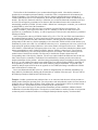
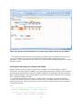
The screen shot in the top half of Fig. 3S1.1 shows how this problem would be formulated with LINGO.
FIGURE 3S1.1 Screen shots showing the LINGO formulation and the
LINGO solution report for a simple linear programming problem.
1 The first line of this formulation is just a comment describing the model. Note that the comment is
preceded by an exclamation point and ended by a semicolon. This is a requirement for all comments in a
LINGO formulation. The second line gives the objective function (without bothering to include the Z
variable) and indicates that it is to be maximized. Note that each multiplication needs to be indicated by an
asterisk. The objective function is ended by a semicolon, as is each of the functional constraints on the next
two lines. The nonegativity constraints are not shown in this formulation because these constraints are
automatically assumed by LINGO. (If some variable x did not have a nonnegative constraint, you would need
to add @FREE(x); at the end of the formulation.)
Variables can be shown as either lowercase or uppercase, because LINGO is case-insensitive. For
example, a variable x1 can be typed in as either x1 or X1. Similarly, words can be either lowercase or
uppercase (or a combination), for clarity, we will use uppercase for all reserved words that have a predefined
meaning in LINGO.
Notice the menu bar at the top of LINGO window in Fig. 3S1.1. The ‘File’ and ‘Edit’ menu items behave
in a standard Windows fashion. To solve a model once it has been entered, click on the red ‘bullseye’ icon.
(If you are using a platform other than a Windows-based PC, instead type the GO command at the colon
prompt and press the enter key.) Before attempting to solve the model, LINGO will first check whether your
model has any syntax errors and, if so, will indicate where they occur. Assuming no such errors, a solver will
begin solving the problem, during which time a solver status window will appear on the screen. When the
solver finishes, a Solution Report will appear on the screen. Note, you can control whether the solution report
appears automatically or not by clicking on LINGO | Options | Interface | Output Level: | Terse/Verbose.
The bottom half of Fig. 3S1.1 shows the solution report for our example. The Value column gives the
optimal values of the decision variables. The first entry in the Slack or Surplus column shows the
corresponding value of the objective function. The next two entries indicate the difference between the two
sides of the respective constraints. The Reduced Cost and Dual Price columns provide some sensitivity
analysis information for the problem. After discussing postoptimality analysis (including sensitivity analysis)
in Sec 4.7 we will explain what reduced costs and dual prices are while describing LINDO in Appendix 4.1.
These quantities provide only a portion of the useful sensitivity analysis information. To generate a full
sensitivity analysis report (such as shown in Appendix 4.1 for LINDO) the Range command in the LINGO
menu would need to be chosen next.
Just as was illustrated with MPL in Sec 3.6, LINGO is designed mainly for efficiently formulating very
large models by simultaneously dealing with all constraints or variables of the same type. We soon will use
the following example to illustrate how LINGO does this.
Example. Consider a production-mix problem where we are concerned with what mix of four products we
should produce during the upcoming week. For each product, each unit produced requires a known amount of
production time on each of three machines. Each machine has a certain number of hours of production time
available per week. Each product provides a certain profit per unit produced.
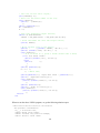
Figure 3S1.2 shows three types of data: machine-related data, product-related data, and data related to
combinations of a machine and product. The objective is to determine how much to produce of each product
so that total profit is maximized while not exceeding the limited production capacity of each machine.
2 Figure 3S1.2 Data needed for the product-mix example.
In standard algebraic form, the structure of the linear programming model for this problem is to choose the
nonnegative production levels (number of units produce during the upcoming week) for the four products so
as to
4
Maximize
∑c x ,
j =1
j
j
subject to
4
∑a x
j =1
ij
j
≤ bi, for i = 1, 2, 3;
where
xj = production level for product P0j,
cj = unit profit for product P0j,
aij = production time on machine i per unit of product P0j,
bi = production time available per week on machine i.
This model is small enough, with just 4 decision variables and 3 functional constraints, that it could be
written out completely, term by term, but it would tedious. In some similar application, there might instead
be hundred of decision variables and functional constraints. So writing out a term-by-term version of this
3 model each week would not be practical. LINGO provides a much more efficient and compact formulation,
comparable to the above summary of the model, as we will see next.
Formulation of the Model in LINGO
This model has a repetitive nature. All the decision variables are of the same type and all the functional
constraints are of the same type. LINGO uses sets to describe this repetitive nature. The simple sets of
interest in this case are
1. The set of machines, {Roll, Cut, Weld}.
2. The set of products, {P01, P02, P03, P04}.
The attributes of interest for the members of these sets are
1. Attribute for each machine: Number of hours of production time available per week.
2. Attributes for each product: Profit per unit produced; Number of units produced per week.
Thus, the first two types of attributes are input data that will become parameters of the model, whereas the
last type (number of units produced per week of the respective products) provides the decision variables for
the model. Let us abbreviate these attributes as follows:
Machine: ProdHoursAvail
Product: Profit, Produce.
One other key type of information is the number of hours of production time that each unit of each product
would use on each of the machines. This number can be viewed as an attribute for the members of the set of
all combinations of a product and a machine. Because this set is derived from the two simple sets, it is
referred to as a derived set. Let us abbreviate the attribute for members of this set as follows.
MaPr( Machine, Product): ProdHoursUsed
A LINGO formulation typically has three sections.
1. A SETS section that specifies the sets and their attributes. You can think of it as describing the structure of
the data.
2. A DATA section that either provides the data to be used or indicates where it is to be obtained.
3. A section that provides the mathematical model itself.
We begin by showing the first two sections for the example below.
! LINGO3h;
! Product mix example;
! Notice: the SETS section says nothing about the number or names of
the machines or products. That information is determined
completely by supplied data;
SETS:
! The simple/primitive sets;
Machine: ProdHoursAvail;
Product: Profit, Produce;
! A derived set;
MaPr( Machine, Product): ProdHoursUsed;
ENDSETS
DATA:
! Get the names of the machines & hours avail;
4 Machine, ProdHoursAvail =
Roll
28
Cut
34
Weld
21;
! Get the names of the products & profits;
Product, Profit =
P01
26
P02
35
P03
25
P04
37;
! Hours needed per unit of product;
ProdHoursUsed = 1.7 2.1 1.4 2.4 ! Roll;
1.1 2.5 1.7 2.6 ! Cut;
1.6 1.3 1.6 0.8; ! Weld;
ENDDATA
Before presenting the mathematical model itself, we need to introduce two key set looping functions that
enable applying an operation to all members of a set by using a single statement. One is the @SUM function,
which computes the sum of an expression over all members of a set. The general form of @SUM is
@SUM( set: expression). For every member of the set, the expression is computed, and then they are
all added up. For example,
@SUM( Product(j): Profit(j)* Product(j))
sums the expression following the colon-the unit profit of a product times the production rate of the productover all members of the set preceding the colon. In particular, because this set is the set of products
{Product(j) for j = 1, 2, 3, 4}, the sum is over the index j. Therefore, this specific @SUM function provides
the objective function,
4
∑c x ,
j =1
j
j
given earlier for the model.
The second key set looping function is the @FOR function. This function is used to generate constraints
over members of a set. The general form is @FOR( set: constraints). For example,
@FOR( Machine(i):
@SUM( Product(j): ProdHoursUsed(i,j)*Produce(j)) <= ProdHoursAvail(i);
says to generate the constraint following the colon for each member of the set preceding the colon. (The “less
than or equal to” symbol, ≤ , is not on the standard keyboard, so LINGO treats the standard keyboard
symbols <= as equivalent to ≤.) This set is the set of machines {Machine(i) for i = 1, 2, 3}, so this function
loops over the index i. For each i, the constraint following the colon was expressed algebraically earlier as
4
∑a x
j =1
ij
j
≤ bi .
Therefore, after the third section of the LINGO formulation (the mathematical model itself) is added, we
obtain the complete formulation shown below:
! LINGO3h;
5 ! Product mix example;
! Notice: the SETS section says nothing about the number or names of
the machines or products. That information is determined
completely by supplied data;
SETS:
! The simple/primitive sets;
Machine: ProdHoursAvail;
Product: Profit, Produce;
! A derived set;
MaPr( Machine, Product): ProdHoursUsed;
ENDSETS
DATA:
! Get the names of the machines & hours avail;
Machine, ProdHoursAvail =
Roll
28
Cut
34
Weld
21;
! Get the names of the products & profits;
Product, Profit =
P01
26
P02
35
P03
25
P04
37;
! Hours needed per unit of product;
ProdHoursUsed = 1.7 2.1 1.4 2.4 ! Roll;
1.1 2.5 1.7 2.6 ! Cut;
1.6 1.3 1.6 0.8; ! Weld;
ENDDATA
! Maximize total profit contribution;
MAX = @SUM( Product(i): Profit(i)*Produce(i));
! For each machine i;
@FOR( Machine(i):
! Hours used <= hours available;
@SUM( Product(j): ProdHoursUsed(i,j)*Produce(j))
<= ProdhoursAvail(i);
);
The model is solved by pressing the ‘bullseye’ button on the LINGO command bar. Pressing the ‘x=’ button
on the command bar produces a report that looks in part as follows.
Global optimal solution found.
Objective value:
Total solver iterations:
Variable
PRODUCE( P01)
PRODUCE( P02)
PRODUCE( P03)
PRODUCE( P04)
Row
1
2
3
4
475.0000
3
Value
0.000000
10.00000
5.000000
0.000000
Slack or Surplus
475.0000
0.000000
0.5000000
0.000000
6 Reduced Cost
3.577922
0.000000
0.000000
1.441558
Dual Price
1.000000
15.25974
0.000000
2.272727
Thus, we should produce 10 units of product P02 and 5 units of product P03, where Row 1 gives the resulting
total profit of 475. Notice that this solution exactly used the available capacity on the first and third
machines (because Rows 2 and 4 give a Slack or Surplus of 0) and leaves the second machine with 0.5 hour
of idleness. (We will discuss reduced costs and dual prices in Appendix 4.1 in conjunction with LINDO and
LINGO.)
The Rows section of this report is slightly ambiguous in that you need to remember that Row 1 in the
model concerns the objective function and the subsequent rows involve the constraints on machine capacities.
This association can be made more clear in the report by giving names to each constraint in the model. This
is done by enclosing the name in [ ], placed just in front of the constraint. See the following modified
fragment of the model.
[TotProf] MAX = @SUM( Product(i): Profit(i)*Produce(i));
! For each machine i;
@FOR( Machine(i):
! Hours used <= hours available;
[Capc] @SUM( Product(j): ProdHoursUsed(i,j)*Produce(j))
<= ProdhoursAvail(i);
);
The solution report now contains these row names.
Row
TOTPROF
CAPC( ROLL)
CAPC( CUT)
CAPC( WELD)
Slack or Surplus
475.000000
0.000000
0.500000
0.000000
Dual Price
1.000000
15.259740
0.000000
2.272727
An important feature of a LINGO model like this one is that it is completely “scalable” in products and
machines. In other words, if you want to solve another version of this product-mix problem with a different
number of machines and products, you would only have to enter the new data in the DATA section. You
would not need to change the SETS section or any of the equations. This conversion could be done by
clerical personnel without any understanding of the model equations.
Scalar vs. Set-Based Models
The above is a “set-based” formulation. For simple models, you may be satisfied with a simpler “scalar”
formulation that does not include the SETS “machinery.” In fact, if for the above model you click on
LINGO | Generate | Display model, you will get the following display of the equivalent scalar model.
MODEL:
[_1] MAX= 26 * PRODUCE_P01 +
+ 25 * PRODUCE_P03 +
[_2] 1.7 * PRODUCE_P01 + 2.1
+ 1.4 * PRODUCE_P03 + 2.4
[_3] 1.1 * PRODUCE_P01 + 2.5
+ 1.7 * PRODUCE_P03 + 2.6
[_4] 1.6 * PRODUCE_P01 + 1.3
+ 1.6 * PRODUCE_P03 + 0.8
END
35 * PRODUCE_P02
37 * PRODUCE_P04
* PRODUCE_P02
* PRODUCE_P04 <=
* PRODUCE_P02
* PRODUCE_P04 <=
* PRODUCE_P02
* PRODUCE_P04 <=
You could in fact enter this simple model in the above form.
7 ;
28 ;
34 ;
21 ;
Importing and Exporting Spreadsheet Data with LINGO
The previous SETS-based example was completely self-contained in the sense that all the data were directly
incorporated into the LINGO formulation. In some other applications, a large body of data will be stored in
some source and will need to be entered into the model from that source. One popular place for storing data is
spreadsheets.
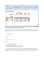
LINGO has a simple function, @OLE( ), for retrieving and placing data from and into spreadsheets. To
illustrate, let us suppose the data for our product-mix problem were originally entered into a spreadsheet as
shown in Fig. 3S1.3. For the moment we are interested only in the shaded cells in columns A-B and E-H.
The data in these cells completely describe our little product-mix example. We want to avoid retyping these
data into our LINGO model. The only part of the LINGO model that needs to be changed is the DATA
section as shown below.
DATA:
! Get the names of the machines & hours avail;
Machine, ProdHoursAvail = @OLE( );
! Get the names of the products & profits;
Product, Profit = @OLE( );
! Hours needed per unit of product;
ProdHoursUsed = @OLE( );
! Send the solution values back;
@OLE( ) = Produce;
ENDDATA
The @OLE( ) function acts as your “plumbing contractor.” It lets the data flow from the spreadsheet to
LINGO and back to the spreadsheet. So-called Object Linking and Embedding (OLE) is a feature of the
Windows operation system. LINGO exploits this feature to make a link between the LINGO model and a
spreadsheet. The first three uses of @OLE( ) above illustrate that this function can be used on the right of an
assignment statement to retrieve data from a spreadsheet. The last use above illustrates that this function can
be placed on the left of an assignment statement to place solution results into the spreadsheet instead. Notice
from Fig 3S1.2 that the optimal solution has been placed back into the spreadsheet in cells E6:H6. One
simple but hidden step that had to be done beforehand in the spreadsheet was to define range names for the
various collections of cells containing the data. Range names can be defined in Excel by using the mouse
and the Insert, Name, Define menu item. For example, the set of cells A9:A11 was given the range name of
Machine. Similarly, the set of cells E4:H4 was given the range name Product.
The above example assumes that the appropriate spreadsheet has been opened in Excel and that this is the
only spreadsheet opened. If you want to make sure that the correct spreadsheet is referenced, or you wish to
retrieve data from several spreadsheets, then you may put the file name in the @OLE( ) argument. For
example, to make sure that the ProdHoursUsed data are retrieved from the file “C:\Hillier9\wbest03i.xls” you
would use the statement:
ProdHoursUsed = @OLE(‘C:\Hillier9\wbest03i.xls’);
in the DATA section.
8 Figure 3S1.3 Screen shot showing data for the product-mix example entered in a spreadsheet.
The LINGO/spreadsheet connection can be pushed even further, so that the LINGO model is stored on a
“tab” in a spreadsheet. Thus, the user may think of the model as residing completely in the single
spreadsheet. One thus can combine the best features of a spreadsheet and a modeling language. (See LINGO
manuals for details.)
Importing and Exporting from a Database with LINGO
Another common repository for data in a large firm is in a database. In a manner similar to @OLE ( ),
LINGO has a connection function, @ODBC( ), for transferring data from and to a databases. This function is
based around the Open DataBase Connectivity (ODBC) standard for communicating with SQL (Structured
Query Language) databases. Most popular databases, such as Oracle, Paradox, DB/2, MS Access, and SQL
Server, support the ODBC convention.
Let us illustrate the ODBC connection for our little product-mix example. Suppose that all the data
describing our problem are stored in a database called acces03j. The modification required in the LINGO
model is almost trivial. Only the Data section needs to be changed, as illustrated by the following fragment
form the LINGO model.
DATA:
! Get the names of the machines & hours avail;
Machine, ProdHoursAvail = @ODBC( 'acces03j');
! Get the names of the products & profits;
Product, Profit = @ODBC( 'acces03j');
9 ! Hours needed per unit of product;
ProdHoursUsed = @OLE( 'acces03j');
! Send the solution values back;
@OLE( 'acces03j') = Produce;
ENDDATA
Notice that, similar to the spreadsheet-based model, the size of the model in terms of the number of variables
and constraints is determined completely by what is found in the database. The LINGO model automatically
adjusts to what is found in the database.
Now let us show what is in the database considered above. It contains three related tables. We give these
tables names to match those in the LINGO model, namely, ‘Machine,’ to hold machine-related data,
‘Product,’ to hold product-related data, and ‘MaPr,’ to hold data related to combinations of machines and
products. Fig. 3S1.4 shows what the tables look like initially on the screen.
Figure 3S1.4 Initial data-base tables for product-mix example.
Notice that the ‘Produce’ column has been initialized to zero in the Product table. Once we solve the model,
the ‘Produce’ amounts get inserted into the database and the Product table looks as in Fig. 3S1.5.
10 Figure 3S1.5 Database tables for product-mix problem after solution.
A complication in using ODBC with Windows is that the user may need to “register” the database with the
“Windows ODBC administrator.” How one does this depends upon the version of Windows. See Windows
documentation for how to do this.
Doing Extra Processing Outside a Model in LINGO The previous LINGO examples illustrated only how to formulate a single model, solve it and produce a
standard solution report. In practice, you may want to a) do some pre-processing of data to prepare it
for your model, b) do some post-processing of a solution to produce a customized solution report, or c)
solve several models automatically in one “run” as part of some comprehensive study. LINGO includes
a programming capability so that you can do (a), (b), and (c). We describe two additional section types,
CALC and SUBMODEL that you can use in LINGO:
CALC:
! Executable statements, perhaps including an
@SOLVE( ) of some submodel;
ENDCALC
11 SUBMODEL Name:
! Constraints describing a specific model;
ENDSUBMODEL
Statements in a CALC section are treated as executable statements rather than constraints. For example,
the statement:
x = x + 1;
is perfectly valid in a CALC section. It means that the value of x should be increased by 1. If the same
statement appeared as part of a model, it would be interpreted as a constraint and the model would be
declared infeasible. You may also use various input and output statements in a CALC section.
The use of a SUBMODEL section allows you to refer to that particular (sub)model in a CALC section.
Thus, in a CALC section you may solve a specific submodel several times with different data, or solve
several different submodels, perhaps using the results from one submodel as input to another submodel.
The programming capabilities of LINGO are illustrated with the following example. We want to
compute a trade-off curve or efficient frontier of risk vs. expected return for a financial portfolio. Notice
that the CALC section: a) does some pre-processing of input data to convert monthly standard
deviations to yearly standard deviations; b) does some post-processing of solution data and uses the
@WRITE statement to generate a customized solution report, and, c) uses the @SOLVE statement to
repeatedly solve the portfolio submodel. Notice in particular the solution report displayed after the
LINGO program.
MODEL:
!Computing an Efficient Frontier for a Portfolio Model in LINGO;
! Generic Markowitz portfolio model in LINGO;
SETS:
! Each asset has an expected return/yr, a standard deviation
in return/month, a standard deviation/yr to be computed,
and an amount to invest to be determined;
ASSET: ERET, STDM, STDY, X;
! Each pair of assets has a correlation. Only store the lower
triangular part;
TMAT( ASSET, ASSET) | &1 #GE# &2: CORR;
ENDSETS
DATA:
! The initial wealth;
WEALTH = 1;
! The investments available(Vanguard funds);
ASSET = CD___
VG040
VG102
VG058
VG079
! Estimated future return per year;
ERET = .04
.06
.06
.05
.065
! Monthly std dev. in return for each asset,
12 VG072
VG533;
.07
.08
;
computed from recent monthly data;
STDM=
0
.02341
.02630
.01067
.02916
.03615
! Correlation matrix, computed from recent monthly data;
CORR =
!CD___;
1
!VG040;
0
1
!VG102;
0
.98209
1
!VG058;
0
-.24279 -.31701
1
!VG079;
0
.75201
.76143
-.34311
1
!VG072;
0
.49386
.49534
-.24055 .68488
1
!VG533;
0
.77011
.76554
-.18415 .84397 .69629
! Number different returns to evaluate;
NPOINTS = 12;
ENDDATA
.05002;
1;
!--------------------------------------------------------------;
SUBMODEL HARRY:
! The standard Markowitz portfolio model;
! Minimize the variance in yearly portfolio return;
[OBJ] MIN = RISK;
RISK = (@SUM( ASSET( I): STDY( I)*STDY(I) * X( I)^2) +
2 * @SUM( TMAT( I, J) | I #NE# J:
X( I) * X( J)* CORR( I, J) *( STDY( I) * STDY( J))))^.5 ;
! Budget constraint;
[BUDGET] @SUM( ASSET(i): X(i)) = WEALTH;
! Return requirement;
[RETURN] @SUM( ASSET(i): ERET(i) * X(i)) >= TARGET * WEALTH;
ENDSUBMODEL
CALC:
! Do some pre-processing of the data;
@FOR( ASSET(I):
! Compute yearly std. dev. from monthly;
STDY(I) = STDM(I)*(12^.5);
);
! Find min and max return over possible investments;
RET_MIN = @MIN( ASSET(I): ERET(I));
RET_MAX = @MAX( ASSET(I): ERET(I));
! Print a heading for risk vs. return trade-off report;
@WRITE(@NEWLINE(1),' Efficient Frontier Portfolio Calculation'
,@NEWLINE(1));
@WRITE(' The possible investments: ',@NEWLINE(1),
'
CD___= risk-free rate, ',@NEWLINE(1) ,
'
VG040= SP500 stock index, ',@NEWLINE(1) ,
'
VG058= Insured long term tax exempt, ',@NEWLINE(1),
'
VG072= Pacific stock index ',@NEWLINE(1),
'
VG079= European Stock index, ',@NEWLINE(1),
'
VG102= Tax managed cap appreciation, ',@NEWLINE(1),
'
VG533= Emerging markets. ' ,@NEWLINE(2) );
@WRITE('
Target
Risk(1 sd)
@WRITE('
Return
1-Yr ');
13 Portfolio composition',
@NEWLINE(1));
! Turn off all but error output;
@SET("TERSEO", 2);
! Write out the asset names in one row;
@FOR( ASSET(I):
@WRITE(' ',ASSET(i));
);
@WRITE( @NEWLINE(1));
N1 = NPOINTS-1;
K = 0;
! Loop over different target returns;
@WHILE( K #LT# NPOINTS:
TARGET = RET_MAX*(K/N1) + RET_MIN*((N1-K)/N1);
! Solve the model for this new target return;
@SOLVE( HARRY);
! Write another line in the report;
@WRITE( '
',@FORMAT( TARGET, '#6.3f'),' ');
@WRITE( @FORMAT( RISK, '#7.4f'),' ');
@FOR( ASSET(I):
! If X is close to 0, print a blank rather than 0.0000;
@IFC( X(i) #GT# .00001:
@WRITE( @FORMAT( X(i), '#7.4f'));
@ELSE
@WRITE('
');
)
);
@WRITE( @NEWLINE(1));
K = K + 1;
); ! While end;
@WRITE(@NEWLINE(1),' Input data used: ',@NEWLINE(1));
@WRITE(' Expected return/yr:');
@FOR( ASSET(I):
@WRITE( @FORMAT( ERET(i), '#7.4f'));
);
@WRITE( @NEWLINE(1));
@WRITE(' Stdev in return/yr:');
@FOR( ASSET(I):
@WRITE( @FORMAT( STDY(i), '#7.4f'));
);
ENDCALC
END
When we run the above LINGO program, we get the following solution report.
Efficient Frontier Portfolio Calculation
The possible investments:
CD___= risk-free rate,
VG040= SP500 stock index,
VG058= Insured long term tax exempt,
VG072= Pacific stock index
14 VG079= European Stock index,
VG102= Tax managed cap appreciation,
VG533= Emerging markets.
Target Risk(1 sd)
Portfolio
Return
1-Yr
CD___ VG040
0.040 0.0000 1.0000
0.044 0.0077 0.7443 0.0062
0.047 0.0154 0.4885 0.0124
0.051 0.0231 0.2328 0.0186
0.055 0.0309
0.0865
0.058 0.0452
0.0626
0.062 0.0635
0.065 0.0831
0.069 0.1035
0.073 0.1244
0.076 0.1457
0.080 0.1733
composition
VG102 VG058
0.0193
0.0386
0.0579
0.0174
0.1815
0.3631
0.5446
0.6898
0.5705
0.4966
0.3874
0.2499
0.1124
VG079
VG072
0.0301
0.0601
0.0902
0.1240
0.1165
0.0655
0.0187
0.0373
0.0560
0.0823
0.1703
0.2301
0.2924
0.3413
0.3902
0.3636
VG533
0.0801
0.2078
0.3202
0.4088
0.4975
0.6364
1.0000
Input data used:
Expected return/yr: 0.0400 0.0600 0.0600 0.0500 0.0650 0.0700 0.0800
Stdev in return/yr: 0.0000 0.0811 0.0911 0.0370 0.1010 0.1252 0.1733
Notice how as the desired or target return is increased, the allocation of funds shifts from the less risky,
lower return investments on the left, to the more risky, higher return investments on the right.
More about LINGO
Only some of the capabilities of LINGO have been illustrated in this supplement. A summary of some of the
additional capabilities beyond solution of simple linear programming problems is:
1) Scalability of models. The SETS/subscripted variables capability allows you to formulate one model
that can be applied to a small problem today, and by only changing the input data, applied to a huge problem
tomorrow.
2) Interface to outside data sources. The examples in this section illustrate that you can retrieve input and
store output for a model from a variety of data sources: spreadsheets, standard text files, and databases.
3) Ability to formulate and solve relatively arbitrary nonlinear problems.
4) Solve problems with integer variables, with either linear or nonlinear constraints.
5) Solve problems with quadratic constraints with extra efficiency.
6) Find and prove global optimality for complex nonlinear models.
7) Programming capability to allow the solution of several related models in a single run.
8) Support for most mathematical functions one might need to use such as trigonometric functions and
most probability functions such as the Normal and Binomial distributions.
LINGO contains extensive built-in documentation. To get to the User Manual when in LINGO, click on
Help | Help topics | Contents | LINGO Users Manual.
Alternatively you may look up terms in the Index by clicking on
Help | Help topics | Index.
15 LINGO is available in a variety of sizes. The version that is included with this text is limited to a maximum
of 150 functional constraints and 300 decision variables. (When dealing with integer programming problems
in Chap. 11 or nonlinear programming problems in Chap. 12, a maximum, of 30 integer variables or 30
nonlinear variables are allowed. In the case of global optimization problems discussed in Sec 12.10, the total
number of nonlinear decision variables cannot exceed 5.) The largest version (called the Extended version) is
limited only by the computer memory available. On a 64 bit computer, linear programs with millions of
variables and constraints have been solved. LINGO is available for most major operating systems, including
Linux.
If you would like to see how LINGO can formulate a possibly huge model like the production planning
example introduced in Sec. 3.6, see the second supplement for this chapter. By reducing the number of
products, plants, machined and months, the supplement also introduces actual data into the formulation and
then shows the complete solution. The supplement goes on to discuss and illustrate the debugging and
verification of this large model. The supplement also describes further how to retrieve data from external
files (include spreadsheets) and how to insert results in existing files.
In addition to this supplement, the additional material on this website includes both a LINGO tutorial and
LINGO/LINDO files with numerous examples of LINGO formulations. These LINGO/LINDO files for
most other chapters include LINGO formulations for problems that are outside the realm of linear
programming. In addition, Sec. 12.10 discusses a global optimization feature of LINGO for dealing with
complicated nonlinear programming problems. Also see Selected References 3 and 5 for Chap. 3 for further
details on LINGO.
16