1
Performance Evaluation of
Mobility Management Protocols
for the Next Generation Internet (IPv6)
Johnny M. Lai
School of Electrical & Computer Systems Engineering
Monash University
Melbourne, Australia
Thesis Submitted for
the Degree of Master of Engineering Science
January 2004
i
Abstract
Internet adoption has surpassed all other communication technologies before it including telephone, radio, television and personal computers. Michael Ritter of Mobility Network Systems puts it succinctly, the Internet “fundamentally provides us
with instant access to all the information ever produced by the human race”.
The drive for always-on Internet access has now entered the mobile domain.
Mobile commerce is the next big thing after electronic commerce. The reason for
this is simple, mobile computing will become the norm for the way people conduct
business, and will become as ubiquitous as the devices that we now take for granted
such as mobile phones, the personal computer and a menagerie of other commonplace
devices that were considered a luxury only a few years ago.
The landscape of today’s telecommunications portrays an amazing patchwork
of heterogeneous networks, with very few and complex bridges between them. In
this context, IP technology has emerged as a natural means of initiating network
convergence as the incumbent telecommunication providers have finally admitted
that using IP as the foundation for next-generation mobile networks makes strong
economic and technical sense.
This drive towards an all-IP infrastructure has already started with the 3rd
Generation (3G) mobile networks, which is aimed at heterogeneous access devices
connected to the same global network, the Internet. Mobile IP (MIP) is the current
method of Internet connectivity for mobile devices. It allows a mobile device to
maintain established communication sessions whilst roaming in different parts of
the Internet. There are two problems with this approach, the limited address space
of IPv4 and the “cumbersome communications process”.
Mobile IPv6 is a current “work in progress” by the Internet’s standardisation
body the IETF. It solves some of the inherent limitations of MIP. However Mobile
IPv6 (MIPv6) still faces the same difficulties when handling real time traffic arising
from multimedia rich applications. The problems stem from the lengthy handover
process at the network layer. There are some handover improvement techniques that
aim to reduce the lengthy handover process.
This research is aimed at evaluating some of these techniques by simulation to
see how close we are to the ideal goal of attributing handover delay to the limitations
of the physical hardware below the network layer.
ii
Acknowledgements
I would like to thank: my supervisors Ahmet Şekercioğlu and Greg Egan for the
encouragement, enthusiasm and direction. My Aunty for cooking up great meals
and letting me stay at her place. My Mother for her dogged persistence in getting
me to complete my degree. I thank my colleagues Eric Wu who was my partner
in the creation of IPv6Suite and Steve Woon a who contributed his time and effort
in assisting Eric in adding IEEE 802.11b wireless interface complete with cross talk.
Linus Torvalds for Linux, Richard Stallman for GNU Emacs, Donald Knuth for
LATEX 2ε , R Development Core Team for R, and last but not least Andras Varga for
OMNeT++ without which this research would not have been possible.
Above all I am GRATEFUL to you LORD for you have never forsaken me.
iii
Declaration
I declare that, to the best of my knowledge, the research described herein is original
except where the work of others is indicated and acknowledged, and that the thesis
has not, in whole or in part, been submitted for any other degree at this or any
other university.
Johnny M. Lai
Melbourne
January 2004
iv
Contents
1 Introduction
1
2 Mobile Internet Access
6
2.1
Mobility Support for IPv4 . . . . . . . . . . . . . . . . . . . . . . . .
9
2.2
Mobility Support in IPv6 . . . . . . . . . . . . . . . . . . . . . . . .
12
2.2.1
IPv6 . . . . . . . . . . . . . . . . . . . . . . . . . . . . . . . .
12
2.2.2
Mobile IPv6 . . . . . . . . . . . . . . . . . . . . . . . . . . . .
18
3 Access Router Localised Handover Extensions
23
3.1
Fast Handovers for Mobile IPv6 . . . . . . . . . . . . . . . . . . . . .
25
3.2
Layer Two “Link Up” Trigger . . . . . . . . . . . . . . . . . . . . . .
30
3.3
Fast Solicited Router Advertisements . . . . . . . . . . . . . . . . . .
30
3.4
Optimistic Duplicate Address Detection . . . . . . . . . . . . . . . .
31
3.5
Previous Care of Address Forwarding . . . . . . . . . . . . . . . . . .
32
4 Localised Mobility Management
35
4.1
Hierarchical Mobile IPv6 . . . . . . . . . . . . . . . . . . . . . . . . .
42
4.2
Fast Handovers in HMIPv6 . . . . . . . . . . . . . . . . . . . . . . .
45
4.3
Local Mobility Agent Selection Algorithms
. . . . . . . . . . . . . .
46
4.4
Other Micromobility Protocols . . . . . . . . . . . . . . . . . . . . .
49
5 Performance Evaluation of Mobile IPv6 Enhancements
52
5.1
IPv6Suite Simulation Framework . . . . . . . . . . . . . . . . . . . .
52
5.2
IPv6Suite Deviations from MIPv6 IETF draft . . . . . . . . . . . . .
54
5.3
Simulation Scenarios . . . . . . . . . . . . . . . . . . . . . . . . . . .
56
5.3.1
Access Router Localised Handover Extensions . . . . . . . . .
58
5.3.2
Previous Care of Address Forwarding . . . . . . . . . . . . .
61
v
5.3.3
Hierarchical Mobile IPv6 . . . . . . . . . . . . . . . . . . . .
6 Discussion of Results
6.1
61
63
Access Router Localised Handover Extensions . . . . . . . . . . . . .
63
6.1.1
Round Trip Time Irregularities . . . . . . . . . . . . . . . . .
68
6.1.2
Optimistic Duplicate Address Detection . . . . . . . . . . . .
70
6.1.3
Fast Solicited Router Advertisements
. . . . . . . . . . . . .
71
6.1.4
Fast RA Beacons . . . . . . . . . . . . . . . . . . . . . . . . .
71
6.1.5
L2 Trigger . . . . . . . . . . . . . . . . . . . . . . . . . . . . .
73
6.1.6
AR Localised Extensions Combined . . . . . . . . . . . . . .
75
6.2
Previous Care of Address Forwarding . . . . . . . . . . . . . . . . . .
77
6.3
Hierarchical Mobile IPv6 . . . . . . . . . . . . . . . . . . . . . . . . .
81
6.4
Problems with Route Optimisation . . . . . . . . . . . . . . . . . . .
92
7 Conclusions and Recommendations for Future Work
94
7.1
Conclusions . . . . . . . . . . . . . . . . . . . . . . . . . . . . . . . .
94
7.2
Recommendations for Future Work . . . . . . . . . . . . . . . . . . .
97
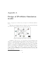
A Design of IPv6Suite Simulation model
98
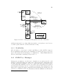
A.1 IPv6Suite Network Layer Modules . . . . . . . . . . . . . . . . . . .
99
A.1.1 RoutingTable6 . . . . . . . . . . . . . . . . . . . . . . . . . .
99
A.1.2 Encapsulation . . . . . . . . . . . . . . . . . . . . . . . . . . .
99
A.1.3 Forwarding . . . . . . . . . . . . . . . . . . . . . . . . . . . .
99
A.1.4 NeighbourDiscovery . . . . . . . . . . . . . . . . . . . . . . .
99
A.1.5 IPv6Mobility . . . . . . . . . . . . . . . . . . . . . . . . . . . 100
A.2 OMNeT++ Messages . . . . . . . . . . . . . . . . . . . . . . . . . . 100
A.3 OMNeT++ patterns . . . . . . . . . . . . . . . . . . . . . . . . . . . 101
A.3.1 Activity to HandleMessage Conversion . . . . . . . . . . . . . 101
A.3.2 Callback pattern . . . . . . . . . . . . . . . . . . . . . . . . . 104
A.3.3 Lifetime Management of Conceptual Data Structures . . . . . 106
A.3.4 Pointer Management . . . . . . . . . . . . . . . . . . . . . . . 106
B Configuration of Simulation
110
B.1 XML Configuration . . . . . . . . . . . . . . . . . . . . . . . . . . . . 110
B.1.1 local element . . . . . . . . . . . . . . . . . . . . . . . . . . . 110
B.2 Libcwd Diagnostic Message Streams . . . . . . . . . . . . . . . . . . 110
vi
B.3 CMake - Cross-Platform Build Configuration Tool . . . . . . . . . . 112
C Interpretation of Box Plot
114
vii
List of Figures
1.1
Years to reach 50 million users worldwide. (Reproduced from [1].) . . .
1
1.2
Internet Protocol Stack . . . . . . . . . . . . . . . . . . . . . . . . .
4
2.1
Routing on the Internet is dependent on the destination IP address
to act as a unique identifier . . . . . . . . . . . . . . . . . . . . . . .
7
2.2
Mobile IP entities . . . . . . . . . . . . . . . . . . . . . . . . . . . . .
8
2.3
Layer two handover scenario . . . . . . . . . . . . . . . . . . . . . . .
9
2.4
Layer three handover scenario. . . . . . . . . . . . . . . . . . . . . .
10
2.5
Triangular routing in MIP . . . . . . . . . . . . . . . . . . . . . . . .
11
2.6
IPv6 address resolution operation . . . . . . . . . . . . . . . . . . . .
15
2.7
Entities involved in IPv6 Encapsulation . . . . . . . . . . . . . . . .
18
2.8
Two modes of communication in Mobile IPv6 . . . . . . . . . . . . .
20
3.1
Handover latency components for Mobile IPv6 . . . . . . . . . . . .
24
3.2
Anticipated Fast Handover operation . . . . . . . . . . . . . . . . . .
25
3.3
Non-anticipated Fast Handover Operation . . . . . . . . . . . . . . .
29
3.4
Previous care-of address Forwarding in action . . . . . . . . . . . . .
33
4.1
MN movement between network segments in the global Internet . . .
37
4.2
Use of LMA in LMM protocols to reduce global bindings . . . . . . .
38
4.3
Conceptual access network architecture . . . . . . . . . . . . . . . .
41
4.4
Typical network configuration for Kawano et. el.’s proposed method
48
4.5
Kawano’s mobility based map selection algorithm in action . . . . .
48
4.6
Time-based binding update in action . . . . . . . . . . . . . . . . . .
50
5.1
AR-local extensions as factors in experiment . . . . . . . . . . . . . .
60
5.2
Handover scenario for AR-local extensions . . . . . . . . . . . . . . .
60
5.3
Simulation scenario with separated router and HA entities. . . . . . .
61
viii
5.4
Simulation scenario for HMIPv6 . . . . . . . . . . . . . . . . . . . . .
62
6.1
Time series plot of round trip time for a single random run of MIPv6
65
6.2
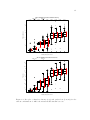
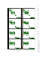
Box plot of ICMP ping round trip time for selected schemes in ARlocal handover extensions experiment . . . . . . . . . . . . . . . . . .
66
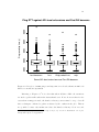
Box plot of handover latency (top) and packet loss (bottom) for the
various combinations of AR-local extensions and fast RA beacons . .
67
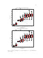
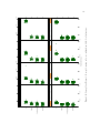
Same plot as Figure 6.3 except the 4th handover i.e. the returning
home case is omitted . . . . . . . . . . . . . . . . . . . . . . . . . . .
69
Time series plot of round trip time for a single random run of MIPv6
with Fast RA beacons. . . . . . . . . . . . . . . . . . . . . . . . . . .
72
6.6
Histograms of ping round trip time for MIPv6 and Fast RA . . . . .
73
6.7
Jitter comparison between MIPv6 and MIPv6 with Fast RA beacons
74
6.8
Plot of end-to-end delay for dInternet of 50ms.
. . . . . . . . . . . .
77
(a)
Plot of end-to-end delay for MIPv6. . . . . . . . . . . . . . . . .
77
(b)
Plot of end-to-end delay for PCoAF. . . . . . . . . . . . . . . .
77
Comparison of handover latency at 1st handover between when PCoAF
is enabled and disabled for MIPv6 and access router (AR)-local extensions combined. . . . . . . . . . . . . . . . . . . . . . . . . . . . . . .
78
6.10 Conditional plot of handover latency (top) and packet loss (bottom)
against handover schemes for different dInternet . . . . . . . . . . . .
79
6.11 Comparison between HMIPv6 and MIPv6 at 1st handover
. . . . . .
82
6.12 Conditional plot of handover latency against handover schemes for
different propagation delays. The lower shingle is dInternet and upper
shingle is dM AP . . . . . . . . . . . . . . . . . . . . . . . . . . . . . .
84
6.13 Conditional plot of HMIPv6 experiment . . . . . . . . . . . . . . . .
85
6.14 Conditional plot of HMIPv6 experiment . . . . . . . . . . . . . . . .
87
A.1 IPv6Suite network layer components . . . . . . . . . . . . . . . . . .
98
6.3
6.4
6.5
6.9
A.2 Flow of datagrams in Encapsulation module of IPv6Suite . . . . . . 100
A.3 Truncated cTimerMessage inheritance diagram . . . . . . . . . . . . 105
B.1 Screenshot of ccmake on IPv6Suite . . . . . . . . . . . . . . . . . . . 113
C.1 Diagram of a box plot showing main features . . . . . . . . . . . . . 115
ix
List of Tables
4.1
Normalized cost of different wireless access technologies . . . . . . .
36
5.1
Common simulation parameters . . . . . . . . . . . . . . . . . . . . .
59
5.2
Parameters for Mobile IPv6 with Fast RA Beacons . . . . . . . . . .
61
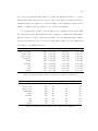
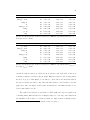
6.1
Mean and CI of handover latency for AR-local extensions . . . . . .
64
6.2
Mean and CI of packet loss for AR-local extensions . . . . . . . . . .
64
6.3
Mean and CI of handover latency for PCoAF experiment with dInternet =
0.01s . . . . . . . . . . . . . . . . . . . . . . . . . . . . . . . . . . . . 80
6.4
Mean and CI of handover latency for PCoAF experiment with dInternet =
0.05s . . . . . . . . . . . . . . . . . . . . . . . . . . . . . . . . . . . . 80
6.5
Mean and CI of handover latency for PCoAF experiment with dInternet =
0.1s . . . . . . . . . . . . . . . . . . . . . . . . . . . . . . . . . . . . 81
6.6
Mean and CI of handover latency for PCoAF experiment with dInternet =
0.5s . . . . . . . . . . . . . . . . . . . . . . . . . . . . . . . . . . . . 81
6.7
Mean and CI of handover latency for HMIPv6 experiment with dinternet =
0.05s and dM obilityAnchorP oint(M AP ) = 0.002s . . . . . . . . . . . . . . 88
6.8
Mean and CI of handover latency for HMIPv6 experiment with dinternet =
0.1s and dM AP = 0.002s . . . . . . . . . . . . . . . . . . . . . . . . . 88
6.9
Mean and CI of handover latency for HMIPv6 experiment with dinternet =
0.2s and dM AP = 0.002s . . . . . . . . . . . . . . . . . . . . . . . . . 89
6.10 Mean and CI of handover latency for HMIPv6 experiment with dinternet =
0.5s and dM AP = 0.002s . . . . . . . . . . . . . . . . . . . . . . . . . 89
6.11 Mean and CI of handover latency for HMIPv6 experiment with dinternet =
0.05s and dM AP = 0.02s . . . . . . . . . . . . . . . . . . . . . . . . . 90
6.12 Mean and CI of handover latency for HMIPv6 experiment with dinternet =
0.1s and dM AP = 0.02s . . . . . . . . . . . . . . . . . . . . . . . . . . 90
6.13 Mean and CI of handover latency for HMIPv6 experiment with dinternet =
0.2s and dM AP = 0.02s . . . . . . . . . . . . . . . . . . . . . . . . . . 91
x
6.14 Mean and CI of handover latency for HMIPv6 experiment with dinternet =
0.5s and dM AP = 0.02s . . . . . . . . . . . . . . . . . . . . . . . . . . 91
A.1 IPv6Suite Primary class Dependencies . . . . . . . . . . . . . . . . .
99
B.1 Features compiled into simulation and the corresponding IPv6Suite
build option . . . . . . . . . . . . . . . . . . . . . . . . . . . . . . . . 112
xi
Listings
A.1 Typical activity function using wait . . . . . . . . . . . . . . . . . . 102
A.2 activity → handleMessage for wait . . . . . . . . . . . . . . . . . . 103
A.3 activity → handleMessage for wait with a waitQueue to handle simultaneous message arrivals . . . . . . . . . . . . . . . . . . . . . . . 104
A.4 activity → handleMessage when receiveNewOn is used . . . . . . . . 104
A.5 Callback pattern . . . . . . . . . . . . . . . . . . . . . . . . . . . . . 105
A.6 cTimerMessageCB Callback method of choice . . . . . . . . . . . 107
A.7 ExpiryEntryList class used in management of entries’ lifetimes . . 108
B.1 XML configuration file used in Section 5.3 . . . . . . . . . . . . . . . 111
xii
Glossary
end-to-end delay The time interval between a packet sent from the sender and
the time it arrived at the receiver. Page ix
home link The link on which a mobile node’s home subnet prefix is defined Page xv
jitter In VoIP, jitter is the variation in inter-arrival times of packets. Page 73
L2 handover A process by which the mobile node changes from one link-layer
connection to another. For example, a change of wireless access point is an L2
handover. Page 9
L3 handover After an L2 handover, a mobile node detects a change in an onlink subnet prefix that would require a change in the primary care-of address.
For example, a change of access router after a change of wireless access point
typically results in an L3 handover. Page 8
round trip time The end-to-end delay plus the time taken for the receiver’s reply
to arrive back at the sender. Page ix
unicast routable address An identifier for a single interface such that a packet
sent to it from another IPv6 subnet is delivered to the interface identified
by that address. Accordingly, such an address must have either a global or
site-local scope but not link-local. Page xiv
xiii
List of Acronyms
3G . . . . . . . . . . . . 3rd Generation Mobile communication technologies with high
transfer rates in the Mbps range and the promise of global coverage.
AAA . . . . . . . . . . Authentication, Authorisation and Accounting
AN . . . . . . . . . . . . access network
Provides access to the Internet.
ANG . . . . . . . . . . access network gateway
AP . . . . . . . . . . . . access point
AR . . . . . . . . . . . . access router A router that exists at the edge of an access network
and through which end users connect to.
ARP . . . . . . . . . . Address Resolution Protocol
BA . . . . . . . . . . . . Binding Acknowledgement
BU . . . . . . . . . . . . Binding Update
CDS . . . . . . . . . . Conceptual Data Structures
CI . . . . . . . . . . . . . confidence interval
CN . . . . . . . . . . . . correspondent node A peer node with which a mobile node is
communicating. The correspondent node may be either mobile or
stationary.
CoA . . . . . . . . . . care-of address A unicast routable address assigned to mobile
node while visiting a foreign link; the subnet prefix of this IP address is a foreign subnet prefix.
DAD . . . . . . . . . . Duplicate Address Detection
DHCP . . . . . . . . Dynamic Host Configuration Protocol
DHCPv6. . . . . . Dynamic Host Configuration Protocol for IPv6
DRL . . . . . . . . . . Default Routers List
DSL . . . . . . . . . . . Digital Subscriber Line
xiv
DTD . . . . . . . . . . Document Type Definition
end-to-end delay The time interval between a packet sent from the sender and
the time it arrived at the receiver.
FA . . . . . . . . . . . . foreign agent
FBACK. . . . . . . Fast Binding Acknowledgement
FBU . . . . . . . . . . Fast Binding Update
FHA . . . . . . . . . . foreign home agent
of the mobile node.
Any home agent that is not on the home link
FMIP . . . . . . . . . Fast Handovers for Mobile IPv6
FSRA . . . . . . . . . Fast Solicited Router Advertisement
HA . . . . . . . . . . . . home agent A router with extra functionality to store the location of the mobile node’s current location and forwards packets to
the mobile node when it is away from home.
HAWAII . . . . . . Handoff-Aware Wireless Access Internet Infrastructure
RR . . . . . . . . . . . . Regional Registration
HMIPv6 . . . . . . Hierarchical Mobile IPv6
HoA . . . . . . . . . . home address A unicast routable address assigned to a mobile
node, used as the permanent address of the mobile node. This
address is within the mobile node’s home link. Standard IP routing
mechanisms will deliver packets destined for the mobile node to its
home link.
IANA . . . . . . . . . Internet Assigned Numbers Authority
ICMP . . . . . . . . . Internet Control Message Protocol
IEEE . . . . . . . . . Institute of Electrical and Electronic Engineers
IETF . . . . . . . . . Internet Engineering Task Force
IPv4 . . . . . . . . . . Internet Protocol Version 4
IPv6 . . . . . . . . . . Internet Protocol Version 6
IPSec . . . . . . . . . IP Security A protocol that provides authentication and encryption over the internet.
IQR . . . . . . . . . . . Inter-Quartile Range
L2 . . . . . . . . . . . . . Layer 2 or Data Link Layer
L2 Trigger . . link up trigger
xv
L3 . . . . . . . . . . . . . Layer 3 or Network Layer
LCoA . . . . . . . . . local care-of address
LMA . . . . . . . . . . Localised Mobility Agent
LMM . . . . . . . . . Localised Mobility Management
LT . . . . . . . . . . . . Location Table
MAP . . . . . . . . . . Mobility Anchor Point
MIP. . . . . . . . . . . Mobile IP An IETF recommendation[2] for MNs to move between
IPv4 subnets without ”interrupting” transport sessions in progress.
MIPv6 . . . . . . . . Mobile IPv6
MIPL . . . . . . . . . Mobile IPv6 for Linux
MM . . . . . . . . . . . Mobility Management
MN . . . . . . . . . . . mobile node A mobile computational device that has wireless IP
connectivity. Synonymous with mobile terminal (MT) and mobile
host (MH) in the literature. Hereinafter referred to as mobile node
for the sake of clarity.
MPLS. . . . . . . . . Multi Protocol Label Switching
NA . . . . . . . . . . . . neigbhour advertisement
NAR . . . . . . . . . . next access router
NAT . . . . . . . . . . Network Address Translation
NCoA . . . . . . . . new care-of address
ND . . . . . . . . . . . . neighbour discovery
NIC . . . . . . . . . . . Network Interface Card
NUD . . . . . . . . . . Neighbour Unreachability Detection
ODAD . . . . . . . . Optimistic Duplicate Address Detection
OMNeT++. . . Objective Modular Network Testbed in C++
PAR . . . . . . . . . . previous access router
PCoA . . . . . . . . . previous care-of address
PCoAF . . . . . . . Previous care-of address Forwarding
PCS. . . . . . . . . . . Personal Communication System
xvi
PDU . . . . . . . . . . Protocol Data Unit
PrRtAdv . . . . . Proxy Router Advertisement
QoS . . . . . . . . . . . Quality of Service
RA . . . . . . . . . . . . Router Advertisement
RBU . . . . . . . . . . Regional Binding Update
RCoA. . . . . . . . . regional care-of address
RFC . . . . . . . . . . Request For Comments
RO . . . . . . . . . . . . Route Optimisation
RS . . . . . . . . . . . . Router Solicitation
RtSolPr . . . . . Router Solicitation for Proxy
SIP . . . . . . . . . . . Session Initiation Protocol
TE . . . . . . . . . . . . Traffic Engineering
UDP . . . . . . . . . . User Datagram Protocol
UML . . . . . . . . . . User Mode Linux
VoIP. . . . . . . . . . Voice over IP
IP packets.
A protocol for encoding and transmitting voice as
WLAN . . . . . . . . Wireless Local Area Network Refers to medium range wireless
communications, typically less than 300 metres[3].
XML . . . . . . . . . . eXtensible Markup Language
xvii
Chapter 1
Introduction
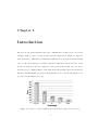
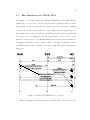
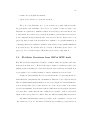
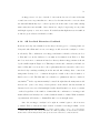
Internet adoption has surpassed all other communication technologies before it including telephone, radio, television and personal computers [4]. Figure 1.1 supports
this observation. Australia’s own Internet traffic has been growing at an astounding
rate: for the six month period ending September 2002 there was an increase of 28%
in data downloaded, and as compared to the previous six month period it was a
42% increase [5]. Michael Ritter of Mobility Network Systems puts it succinctly, the
Internet “fundamentally provides us with instant access to all the information ever
produced by the human race” [6].
Figure 1.1: Years to reach 50 million users worldwide. (Reproduced from [1].)
1
2
The drive for always-on Internet access has now entered the mobile domain.
Mobile commerce is the next big thing after electronic commerce [7, xv-xxi], because
these services should be accessible from anywhere, not just some fixed location like
your bedroom, school computer lab or Internet Cafe. Picture this scenario where
you are to meet a client at 2pm but you are not familiar with this section of the city.
It is 1:50 now. If you were sitting in front of your computer you would be able to
leverage the computing and communication resources in the form of location based
services to locate the meeting place. However, these services are not available at the
time and place when you need them.
Mobile commerce is important because this technological revolution will
directly or indirectly affect in a significant way practically every person
in the industrialised world [7, xv-xxi].
The reason for this is that mobile computing will become the norm for the way
people conduct business, and will become as ubiquitous as the devices that we now
take for granted such as mobile phones, the personal computer and a menagerie of
other commonplace devices that were considered a luxury only a few years ago.
The landscape of today’s telecommunications portrays an amazing patchwork
of heterogeneous networks, with very few and complex bridges between them. In
this context, IP technology has emerged as a natural means of initiating network
convergence as the incumbent telecommunication providers have finally admitted
that
using IP as the foundation for next-generation mobile networks makes
strong economic and technical sense, since it takes advantage of the ubiquitous installed IP infrastructure, capitalises on the Internet Engineering
Task Force (IETF) standardisation process, and benefits from both existing and emerging IP-related technologies and services [8].
3
This drive towards an all-IP1 infrastructure has already started with the 3G
mobile networks, which is aimed at heterogeneous access devices connected to the
same global network, the Internet [9].
Mobile IP [2] is the current method of Internet connectivity for mobile devices.
It allows a mobile device to maintain established communication sessions whilst
roaming in different parts of the Internet. However, there are two major shortcomings when faced with the continual proliferation of mobile devices seeking access
to the Internet. According to Jyrki Halttunen, vice president for Nokia Networks
Asia-Pacific, “more mobile phones than computers will connect to the Internet this
year (2003)” [10]. The first problem is the limited address space of IPv4 [10, 11, 12].
The second problem is the “cumbersome communications process” [10, 8].
The issue of limited address space has been addressed by the gradual transition
to the Next Generation Internet also known as Internet Protocol Version 6 (IPv6)
[13, 14]. IPv6 has an expanded address space.
340 undecillion (340×1036 ) unique addresses which translates to approximately 6.5 × 1024 addresses per square meter of Earth [15].
This is not its only advantage: it supports integrated security and prescribes IP
Security (IPSec) as the Public Key Infrastructure protocol for distribution of keys.
NTT in Japan is already offering dual stack Internet access [15] and full support
for IPv6 exists in common operating systems such as Microsoft Windows XPTM ,
LinuxTM , and the Sony PlaystationTM .
Mobile IPv6 is a current “work in progress” by the Internet’s standardisation
body the IETF [16]. It solves some of the inherent limitations of MIP as described
in Section 2.2. However MIPv6 still faces the same difficulties when handling real
time traffic arising from multimedia rich applications. The problems stem from the
1
Basically a network that contains IP-based transport, multimedia services, and the integration
of IETF protocols such as Mobile IP for wide-area mobility, Session Initiation Protocol (SIP) for
signalling, and Diameter for Authentication, Authorisation and Accounting (AAA) [8].
4
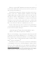
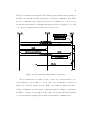
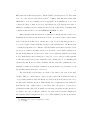
lengthy handover process at the IP layer i.e. layer 3 in the TCP/IP protocol stack
as shown in Figure 1.2. The mobile node (MN) is unable to communicate during
Figure 1.2: Internet Protocol Stack
handover with its peer because any packets sent to the MN at this stage are unable
to reach it since the MN is no longer at its previous location. Nor can the MN send
packets to its peer as it needs to acquire a new IP address before it can notify the
peer node with its new location. The longer the handover process, the greater the
number of packets dropped. There are some handover improvement techniques that
aim to reduce the lengthy handover process. This research is aimed at evaluating
some of these techniques by simulation to see how close we are to the ideal goal of
attributing handover delay to the limitations of the physical hardware below the IP
layer.
By solving the problem of IP mobility for multimedia and real time applications, we will be one step closer to fulfilling the promise of nomadic computing2 as
described by Kleinrock [17] and also the grand vision of pervasive computing [18], a
natural extension to the culmination of computing and communications, where intelligent devices are embedded in a non-intrusive manner in our everyday surroundings,
working collectively to provide us with advanced services.
2
A personalised and customised service available anywhere, on any terminal or via any access
technology.
5
The next chapter provides a detailed view of Mobile IPv6, as that is the IETF
endorsed standard for mobility support in the Next Generation Internet. It introduces the problem of the lengthy delay in IP handover, and is followed by a more
thorough treatment at the start of Chapter 3. The following two chapters describe
the prospective solutions in the current literature: Chapter 3 is a survey of some
access router localised handover extensions, and Chapter 4 is a survey of current
Localised Mobility Management (LMM) protocols. Chapter 5 introduces the simulation model, and how the various simulation scenarios are setup to evaluate the
performance of MIPv6 together with AR-local handover extensions and Hierarchical
Mobile IPv6 (HMIPv6), a specific LMM solution. Chapter 6 analyses and discusses
the simulation results. Chapter 7 concludes this thesis with some recommendations
for future research.
Chapter 2
Mobile Internet Access
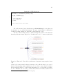
To send packets in the Internet, you need to know who to send them to. This is
analogous with sending a letter to a friend where you have to know their address [19].
The IP address serves as a unique endpoint identifier for a node on the Internet and
is used by Internet applications to specify who to establish a communication session
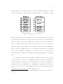
with. Generally speaking the routing of packets on the Internet is also dependent
upon the IP address of the destination as shown in Figure 2.1. Part of that IP
address, its prefix specifies the subnet that the node exists on and routers use this
information to determine the next hop for the packet. Thus an IP address also serves
as a location identifier to enable packets to be routed. Whenever a node moves to
a different point of attachment i.e. different subnet it is assigned with a different
address to reflect its new location. The node is no longer associated with its original
IP address and packets destined for the original IP address are lost.
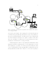
To cater for terminal mobility the idea of visited domains was introduced from
mobile telephony, and so Mobile IP [2] as ratified by the IETF in Request For Comments (RFC) 2002 came into existence. This protocol differentiates between the
roles of the location and endpoint identifiers. The endpoint identifier is the home
address (HoA) which acts as a node’s permanent address. When the MN moves to a
different subnet as shown in Figure 2.2 it will acquire a care-of address (CoA) that
6
7
Sender
Router
dest=A.B.C.D
A.B.C.X
Router
A.X.X.X
Router
A.B.X.X
Router
A.B.C.D
Receiver
Figure 2.1: Routing on the Internet is dependent on the destination IP address to
act as a unique identifier
serves as its location identifier. After acquiring the CoA, the MN will register the
CoA with the home agent (HA). Any packets that were going to the HoA will now be
intercepted by the HA and tunnelled to the MN at its new location. Thus Mobile IP
solved the mobility issue by allowing nodes to always be reachable no matter where
their point of attachment to the Internet was. To put it succinctly, the problem of
mobility has been transformed into a routing problem [20].
Mobility management consists of location management which includes address
management and handover management [21]. Location management is concerned
with acquiring the topologically correct address (CoA) and updating the current
location of the MN with the mobility agent (HA). Handover management is involved
with algorithms that determine when to handover to a new location depending on
8
Figure 2.2: Mobile IP entities
different conditions like missed router advertisements1 , differing advertised network
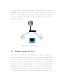
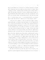
prefix and L2 triggers2 [22]. Handovers can occur at either layer two or layer three.
An Layer 2 or Data Link Layer (L2) handover3 as shown in Figure 2.3, occurs
when the two access points are connected to the same interface on an AR via a
switch or hub. This only involves link segment specific handover procedures e.g.
re-authentication with a new base station in Institute of Electrical and Electronic
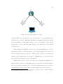
Engineers (IEEE) 802.11b. In an L3 handover
4
there is a change in the point
of attachment to a different subnet and hence either a different AR or different
interface in the same AR. The result is the acquisition of a new IP address which
becomes the node’s new CoA. The L3 handover is the same5 regardless of the link
1
the only mechanism defined for MIPv6
based on layer 2 received signal strength threshold
3
also known as link layer mobility
4
also known as IP mobility
5
in this research there is only one type of L3 handover as dictated by MIPv6
2
9
layer technology used, although certain hints from specific link layer technologies
like IEEE 802.11b can help to reduce handover times as demonstrated in [23]. An
L3 handover always implies an L2 handover as shown in Figure 2.4 although the
reverse is not always true. For further details on the components of an L3 handover
please turn to Chapter 3.
AR
Linux
Linux
AP
AP
MN
Figure 2.3: Layer two handover scenario
2.1
Mobility Support for IPv4
MIP works at the network layer of the TCP/IP protocol stack. It requires mobile
agent functionality in the network provided by a server with home agent (HA) functionality on the home subnet and a similar entity known as a foreign agent (FA)
in a foreign or visited subnet. These servers can be situated on routers. The MN
acquires a CoA from the foreign agent (FA) or another mechanism like Dynamic Host
Configuration Protocol (DHCP) can create a colocated CoA (coCoA). If using the
foreign agent’s CoA then packets are tunnelled by the HA to the FA while using the
coCoA the tunnel reaches all the way to the MN itself. When the MN wants to send
10
AR
Linux
Linux
AP
AP
MN
Figure 2.4: Layer three handover scenario.
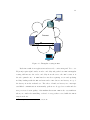
a reply it will send it out directly to the correspondent node (CN) using the home
address as source address. This causes the infamous triangular routing problem [24]
as shown in Figure 2.5, that makes it hard for end to end Quality of Service (QoS)
provisioning to work because the path travelled by the packets is not the same in
both directions.
Theoretically an established connection at a site with MIP support does not
break when moving to a different subnet, even one with different access technology
from the transport layer’s perspective. This is made possible by preserving the
transport layer application’s end points for communication i.e. the HoA as the
network layer uses a different point of attachment.
While MIP was able to solve the problem of node mobility by assigning a permanent address to the node and mapping that to its current location in the Internet,
there are performance implications to consider if seamless handovers6 are required.
Seamless handovers are required when real time traffic traverses the network.
6
A handover in which there is no change in service capability, security, or quality. In practice,
some degradation in service is to be expected [25].
11
CN
Internet
HA
FA
MN
Figure 2.5: Triangular routing in MIP
Real time traffic from applications such as video conferencing and Voice over
IP (VoIP) require tight bounds on end-to-end delay and packet loss. MIP’s triangular
routing will increase the end-to-end delay from the CN to the HA because it is
the sub-optimal route. A MIP handover involves acquiring a CoA and updating
mobility bindings with the HA and CNs7 and so introduces some latency on top of
the latency from the L2 handover. The effect of handover latency is to interrupt
established communications momentarily, packets are dropped as a result and the
user perceives a loss in quality of the multimedia stream. MIP is also very inefficient
when you consider the tunnelling overhead of every packet received while the MN is
away from home.
7
route optimisation is an extension to Mobile IP
12
This is a very active area of research because the global mobile phone market is
currently transitioning to 3G. There have been many proposals that extend MIP and
alternative mobility management protocols [26, 20, 27, 28] with the aim of reducing
the handover latency8 and signalling overhead. However, the common consensus is
that Mobile IPv6 (MIPv6) is the base standard for mobility in next generation IP
networks [10, 8].
2.2
2.2.1
Mobility Support in IPv6
IPv6
The Next Generation Internet protocol (IPv6), is as its name suggests, the next
generation protocol for the Internet that was ratified in 1995 [13]. IPv6 was created to solve the inherent limitations of the current Internet Protocol IPv4. The
most publicised limitation was the uneven distribution of global IP addresses particularly favouring the United States of America9 [12]. Consider the case of Stanford
University in America has more publicly allocated IP addresses than the whole of
China. According to Uti Rahamim VP of sales at Hitachi Internetworking, public
IP addresses could run out as early as 2005. Dr. Paul Francis credited with the
proposal for Network Address Translation (NAT) claims that NAT10 extends IPv4
address from 32 to 4811 bits effectively [12]. While NAT allows more people to surf
the Net and view their e-mails, it fails to provide global routability. So peer to peer
applications like Microsoft’s NetMeeting will not work. To overcome this problem
a server is needed to arbitrate between clients which defeats the purpose of peer
to peer applications. NAT still does not solve the uneven distribution of global IP
8
henceforth this term shall be taken to mean L3 handover latency unless stated otherwise
over 70%
10
also known as port mapping
11
Theoretical maximum derived from maximum number of network ports used by NAT on a
computer which is 216 . It is theoretical because not all the ports can be used for NAT e.g. Internet
Assigned Numbers Authority (IANA) reserved ports in the range 1-1024 inclusive, just like not all
32 bits in an IP address can form public IP addresses
9
13
addresses.
Others have felt that NAT was at best a band-aid solution and waited till
something better to arrive. IPv6 has 128 bit IP addresses, and is available now.
Many organisations have tried to increase the uptake of IPv6 . The EU has invested
55M Euro in a live IPv6 network such as 6Net12 in an attempt to speed up migration
to IPv6 and break the cycle of wondering whether should the network be built first
to test applications or applications built first before the network rolls out, because
investment in network infrastructure without applications is expensive according to
Cisco’s Falkner [12]. 3GPP a global standards body for 3G cellular networks has
mandated UMTS Release 5 for IMS (Internet Multimedia Service) protocols operate
on IPv6 only [12, 11]. Without a doubt the global transition to IPv6 is inevitable.
The following is a brief list of advantages IPv6 has over IPv4 [29]:
• larger address space 2128 compared to IPv4’s 232
• an in-built mechanism to automatically configure the network interfaces13 [30]
• globally unique and hierarchical addressing [31] based on prefixes rather than
address classes, to keep routing tables small and backbone routing efficient14
• supports encapsulation of other protocols as well as itself [33]
• improved multicast routing support (in preference to broadcasting)
• built-in authentication via AH (Authentication Header) and encryption in
terms of ESP (Encapsulated Security Payload) [13]
• inherent support for mobility, MIPv6 is implemented with destination options
which are an integral part of IPv6 [8].
12
www.6net.org
Separate from DHCP (Dynamic Host Configuration Protocol)
14
Instead of IPv4 having over 2 million routes in core routers you only have a maximum of 8,192
derived from the 13 bits for the TLA (Top Level Aggregation) field in an IPv6 address [32]
13
14
2.2.1.1
Address Resolution
IP addresses are abstract addresses that network administrators assign or are derived
from the autoconfiguration process described in Section 2.2.1.2. Each IP address is
mapped to the Network Interface Card’s link-layer address which is programmed
into the Network Interface Card (NIC) during manufacture and is guaranteed to be
sufficiently unique. To determine the link-layer address from an IP address of a host
residing on the same link, a process known as address resolution is carried out in
order for packets to be delivered to the correct node.
In IPv4, the Address Resolution Protocol (ARP) operated in the data link layer
of the TCP/IP protocol stack as shown in Figure 1.2. The “equivalent” functionality
in IPv6 is provided by neighbour discovery which operates from the network layer and
replaces ARP. This mechanism is defined in RFC 2461 Neighbour Discovery of IPv6
[34]. Neighbour discovery as its name implies, is for determining the existence of
neighbouring hosts on the local subnet and their corresponding link-layer addresses.
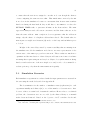
When a node A wants to send a packet to node B on the same link as shown
in Figure 2.6, it will send a neighbour solicitation. This packet is addressed to
a special multicast group formed from B’s IP address. This is known as the solicited multicast address [31]. The packet contains A’s link-layer address in the
source link-layer address option. This allows B to send a unicast neighbour advertisement back to A. Node A will wait for B’s neighbour advertisement for at
least MAX MULTICAST SOLICIT15 *RetransTimer seconds with a neighbour solicitation resent when RetransTimer16 seconds have elapsed. When B receives the
multicast neighbour solicitation, it will put its link-layer address into a target linklayer address option and place that into a neighbour advertisement to be sent directly
back to A. Before A receives the neighbour advertisement any other packets that
are destined for B will be placed into a queue for packets that are pending address
15
16
default three times [34]
default of one second [34]
15
resolution to B. After the neighbour advertisement arrives at A, A can send all the
pending packets in the queue and adds the link-layer address mapping to B’s IP
address to the neighbour cache. Any future packets addressed to B’s IP address will
find B’s link-layer address directly from the neighbour cache.
A
B
RetransTimer
RetransTimer*MaxMulticastSolicit
NS to B ’s Solicited Address
NS to B ’s Solicited Address
...
NA with Link Layer Address
Data
Figure 2.6: IPv6 address resolution operation
2.2.1.2
Autoconfiguration
IPv4 networks required either a network administrator or the presence of a DHCP
server to assign an IP addresses. IPv6 has a configuration mechanism implemented
by all conforming nodes called Stateless Address Autoconfiguration [30] that allows
a node to automatically assign a suitable address for itself.
Autoconfiguration consists of two processes Duplicate Address Detection (DAD)
and Router Discovery. A node is able to self configure based on the premise that
16
its network interface is a unique identifier. The first address that all nodes using
autoconfiguration self assign is the link-local address. This consists of a link-local
prefix FE80:0:0:0:0:0:0:0/64 [31] prepended to the interface identifier17 . The
link-local prefix is only recognised within the scope of the link which means that
routers will not forward these packets. The link-local address goes through DAD
first before been assigned to ensure that no other node has the same link-local
address. At the same time the node can initiate router discovery in order to allow
the node to start communicating as soon as DAD is finished.
The un/solicited router advertisement contains prefixes and each is inspected
for the autoconfiguration flag. If this flag is set then the prefix is combined with
the interface identifier to form other addresses e.g. a globally scoped address so the
node can communicate on the Internet. Usually DAD is only done on the link-local
address because every other address is formed from the interface identifier that has
been tested to be unique on that link when the link-local address was self-assigned.
Likewise the prefixes advertised by the router should be unique within their scope,
because they are configured by the network administrator.
2.2.1.3
Router Discovery
The function of Router Discovery in IPv6 is to allow the non-router nodes to both
solicit and process received un/solicited router advertisements. The routers will send
unsolicited advertisements separated by a time interval that is uniformly distributed
between MIN RTR ADV INT and MAX RTR ADV INT. Once a router is discovered on the network it is added to the Default Routers List (DRL). The DRL stores
the list of routers that the node can forward off-link packets to. If there are no
routers on the network then every address is considered to be on-link [34]. Upon
reception of an advertisement by a node, the prefixes advertised by the router are
searched and if the on-link flag is set for a prefix then that prefix is added to the
17
a MAC address for Ethernet links
17
node’s prefix list. The on-link prefixes in this list are compared against destination
addresses of packets to be sent. Addresses that match the prefix are actually on-link
and these packets can be sent directly to a neighbouring node without the router’s
intervention.
The DRL and on-link prefixes list are Conceptual Data Structures (CDS) used in
the conceptual sending algorithm. It is an algorithm that all nodes use to determine
how to forward or send a packet.
2.2.1.4
Encapsulation
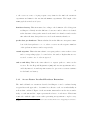
Encapsulation is the process of putting an IPv6/4 datagram as the payload of another IPv6 datagram [33]. The purposes for doing this are many but usually it is
to deliver packets to destinations that are not reachable using normal forwarding
methods. Encapsulation in general involves four parties, the original source A and
destination B of the packet along with the tunnel entry point C and exit point D as
shown in Figure 2.7. The tunnel entry point is where the original datagram from A
is encapsulated into another datagram with the source address of C and destination
of D. The packet is decapsulated18 at tunnel exit point D and forwarded to its final
destination B without modification. The packet arrives at B and appears to have
originated from A. B does not know that the datagram traversed the tunnel C-D.
Thus encapsulation is a non invasive forwarding mechanism to supplement normal
packet forwarding done by routers. A tunnel is unidirectional so to go in the reverse
direction from B to A via the tunnel D-C will require the reverse tunnel D-C to be
established first.
The tunnel destination D and original destination B can be the same node. An
example of this occurs in MIPv6 when the HA intercepts a packet from the CN (A)
destined for the MN at its HoA (B) and encapsulates it with a tunnel source of the
HA’s address (C) and tunnel destination of MN’s CoA (D). The reverse tunnel which
18
the original datagram is extracted from the encapsulating datagram
18
is a tunnel in the opposite direction where the MN is both the tunnel source (C) and
the original source (A) sends a packet to the CN (B) via the HA (D). This is known
as the reverse tunnelling procedure in MIPv6.
B
A
Datagram from A inside
C
src=A
dest=B
D
src=C
dest=D
Tunnel
Tunnel Entry Point
Tunnel Exit Point src=A
dest=B
Note: Intermediate Links not shown
Figure 2.7: Entities involved in IPv6 Encapsulation
2.2.2
Mobile IPv6
Mobile IPv6 [16] is the same in concept as MIP without MIP’s disadvantages. The
advantages of MIPv6 over MIP were mentioned briefly in Chapter 1 where it was
mentioned that MIP used a “cumbersome communications process”. This can be
seen as a reference to the triangular routing problem which was described already at
Section 2.1, the use of tunnelling, and topologically incorrect source address when
away from home subnet. While MIP can overcome the triangular routing problem
using the reverse tunnelling procedure described above, reverse tunnelling is quite
inefficient because of the overhead arising from the extra IP datagram header and
the extra decapsulation and forwarding load at the HA. There is a route optimisation extension to MIP that can also eliminate triangular routing but due to the
limitations of Internet Protocol Version 4 (IPv4) it still uses encapsulation [28, 8]
to deliver packets to the MN directly. The topologically incorrect source address in
19
MIP, the HoA is used by the MN when sending packets. These packets are usually
dropped because a security conscious network adminstrator will have enabled the
routers’ ingress filtering, so that only packets with topologically correct (according
to a predetermined policy) source addresses are forwarded. All of these problems
are solved by MIPv6 as explained below.
IPv6 inherently supports mobility with the autoconfiguration feature. This
eliminates the need for explicit FAs on foreign links as the MN can use normal
Router Advertisement (RA)s to acquire a CoA. The only change required to support
MIPv6 in routers is for them to include an R bit in a prefix information option of
their router advertisement. This prefix includes the router’s global unicast address
and is the prefix used by the MN to configure its CoA to ensure that it is globally
reachable from the Internet.
There are two modes of communication in MIPv6. The default mode uses
tunnelling via the HA while the preferred mode is a direct route established with a
procedure called route optimisation. Both methods are shown in Figure 2.8. Unlike
MIP, triangular routing is not a method of communication although this can occur
momentarily during the transition phase between the two different modes.
2.2.2.1
Interception of Datagrams for Tunnelling by HA
While the MN is away from home, the HA it has a legal mobility binding with will
act as its proxy. This means that any datagrams addressed to the MN will end up
at the HA because the HA will respond to all neighbour solicitation requests for the
MN.
Once the HA has intercepted a datagram, it will forward it to the MN at its
current location, the CoA obtained from the binding cache entry for the MN. The
binding cache entry was created when the MN registered with the HA and is updated
by further Binding Update (BU)s from the MN. The tunnel header will have a source
20
dest=HoA
T2RH=HoA CN
dest=CoA
CN
src=HoA
src=HA
dest=CoA
HA
src=CoA
HDO=HoA
src=CoA
dest=HA
MN
MN
T2RH := Type−2 Routing Header
HDO := Home Destination Option
Figure 2.8: Two modes of communication in Mobile IPv6
address of the HA’s global router address as advertised in its prefix information
option and destination address of the MN’s CoA. The MN decapsulates the datagram
upon arrival resulting in the original datagram, as if the CN had sent it directly to
the MN.
When an MN has not established a binding with its CN, it should send the
datagrams destined to the CN via the HA using the reverse tunnelling procedure.
The original datagram has a source address of HoA and destination address of the
CN while the tunnel’s source address is the MN’s CoA and the destination is the
HA’s global router address. Once the HA receives this packet it will check that
the tunnel’s source address is indeed the CoA corresponding to the HoA from the
original datagram’s source address to prevent other nodes from masquerading as the
MN before forwarding the original datagram. Thus when the datagram arrives at
21
the CN it looks like the MN had sent it from its home subnet.
2.2.2.2
Direct communication using Route Optimisation
MIPv6 does not require tunnelling between the MN and the CN when in the route
optimised mode of communication thanks to the ingenious use of the home address
destination option and type-2 routing header. The two are a substitute for the
function of the endpoint identifier provided by the encapsulation mechanism but
with the overhead reduced to a minimum. The home address destination option
from the MN contains the home address. This allows an MN to send datagrams
with a source address of CoA which is topologically correct in the foreign domain
and so passes the access router’s ingress filtering rules. When the datagram arrives,
the CN will process the home address destination option by swapping the home
address in the option with the datagram’s source address. The modified datagram
is passed on to the transport layer and so the application is not even aware that
it is communicating with a mobile entity. A similar process occurs in reverse when
the CN is to send a datagram to the MN. The application addresses the packet to
the MN at its HoA. At the network layer the CN will inspect its binding cache to
discover the MN’s current location i.e. its CoA as reported by the last BU from the
MN. It will add a type-2 routing header to the datagram with the HoA and replace
the source address with the CoA. The packet will travel through the network using
normal procedures and arrives at the MN. The MN will process the type-2 routing
header by swapping its contents with the source address of the datagram. Thus the
final datagram passed to the transport layer has HoA as the source address. This
keeps applications ignorant of the node’s movement.
To establish a direct route, the MN needs to send a BU to the CN containing
the MN’s current CoA. This will be stored by the CN in its binding cache. In order to prevent malicious nodes from masquerading as a certain MN by sending BU
with HoA of the MN, the return routability procedure is used to verify the nodes au-
22
thenticity. The following explanation provides a very simplified view that omits the
mathematical functions and protocol details, for further information please consult
[16]. The first step is for the MN to send an initiation message to the CN to start
the return routability procedure. The CN will then send a test packet on each of the
two different routes, one via the HA using the HoA as destination while the other
uses the CoA as destination. The two test packets contain parts of a one time cookie
that are assembled at the MN and sent back to the CN. Unless the initiating node
is at the location specified by the CoA is also the owner of HoA, it cannot receive
both parts of the secret token. This is based on the assumption that the HA has
adequately authenticated the MN’s identity. This is a valid assumption as MIPv6
has mandated the use of IPSec authentication in binding updates from the MN to
the HA. Thus return routability will add an extra one and a half roundtrips per CN
that is to be route optimised.
When it comes to handling real time traffic MIPv6 addresses better than MIP
the requirements for stringent end to end delays, because it does not use triangular
routing at all and stipulates that the route optimised mode be used unless the CN
is administratively prohibited from doing so. However, the requirements on packet
loss are not satisfied yet due to the long handover latency of over 2 seconds [35].
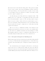
Chapter 3
Access Router Localised
Handover Extensions
Handover latency is defined as the interval starting from the moment when the
mobile node leaves the old access medium until it resumes communication with the
CN at the new access medium [36]. This is shown in Figure 3.1. There are three
components to handover latency. The first D1 is the L2 handover latency i.e. the link
layer specific handover procedure. In the scenario shown it is the 802.11b handover
procedure to switch to a new access point. D2 is the time taken by the MN to detect
the presence of a new AR at the new access network and configure a new CoA. This
is also known as the rendezvous time delay [22]. Rendezvous time is affected by the
amount of overlap or distance between the two neighbouring coverage areas of the
access point (AP)s, the speed of the mobile node and the rate of unsolicited Router
Advertisement (RA) beacons [8, 9]. The third component D3 is the time it takes to
send a BU back to the HA/CN and the subsequent resumption of communications
indicated by a new data packet arriving at the MN from the new AR. This is also
known as the registration delay.
L2 handovers are not discussed any further in this paper as they depend on the
23
24
Figure 3.1: Handover latency components for Mobile IPv6
specific physical transport technology and nothing can be done to alter its behaviour
at the network layer. The rendezvous time is affected by the frequency of router
advertisements. Registration delay is affected by the path delay and packet loss of
the path the BU takes from the MN to the HA in the Internet.
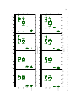
There are basically two varieties of handover management techniques, predictive
and non-predictive [23]. The predictive varieties tend to require assistance from the
network infrastructure, functionality that is usually not built into the system. It is
predictive because it predicts which wireless link and hence subnet the MN will move
to before the actual handover. Non-predictive handovers in general do not require
special assistance from the wired infrastructure and are reactive in nature i.e. it
will perform an L3 handover only after it has detected a transition to a different L3
subnet. As a general rule of thumb predictive handovers are much more complex to
implement and manage.
25
3.1
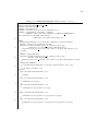
Fast Handovers for Mobile IPv6
An example of a predictive handover technique is Fast Handovers for Mobile IPv6
(FMIP) [37]. It can reduce both the rendezvous and registration delay by anticipating handover before it happens and carrying out some of the time consuming
operations before the actual L2 handover occurs. This requires modifications to the
ARs. FMIP forms a temporary tunnel between the previous access router (PAR) and
the next access router (NAR), thereby allowing the MN to receive packets at the
NAR’s access network before the MN has finished its registration and established it-
self with the NAR. There are three stages to this process: handover initiation, tunnel
establishment and packet forwarding, abbreviated as HI, TE and PF respectively in
Figure 3.2.
Figure 3.2: Anticipated Fast Handover operation
Handover initiation is usually initiated by the MN. The coverage area of the
26
two ARs have to overlap in order for anticipated fast handover to occur1 (The nonanticipated case as supported by 802.11b access networks out of the box shall be
discussed next). The MN knows that it should handover to NAR when it receives
a L2 indication usually called an L2 trigger2 due to perhaps waning received signal
strength from PAR below some threshold level or other factors unrelated to link
quality. The MN sends a Router Solicitation for Proxy (RtSolPr) to its current AR
i.e. PAR with the link layer identifier of the prospective access point e.g. base
station ID. This information is provided by the specific L2 technology. The PAR
responds by sending a Proxy Router Advertisement (PrRtAdv) with the NAR’s link
layer address, its IP address and also any network prefixes to enable the MN to
generate a suitable new care-of address (NCoA) on the new link. If the network is
the one to initiate the handover then it will send an unsolicited PrRtAdv to the MN.
Tunnel establishment involves the MN sending a Fast Binding Update (FBU)
some time after receiving the PrRtAdv3 . Once PAR receives FBU, it will send a
Handover Initiate (HI) to NAR. The purpose of HI is to establish a bidirectional
tunnel between PAR and NAR to allow use of the previous care-of address (PCoA)
on NAR’s link as well as to validate whether the NCoA is valid and unique at
NAR’s link. When NAR receives HI it will set up a host route for MN’s PCoA
by creating a neighbour cache entry that points to PCoA with state of STALE i.e.
address resolution required. NAR should also defend NCoA via proxy neighbour
advertisement for a short period of time after verifying uniqueness of NCoA. NAR
sends back a Handover Acknowledge (HACK) to PAR. PAR will subsequently send
a Fast Binding Acknowledgement (FBACK) to MN. Upon receiving FBACK, the MN
will know that it has permission to use NCoA on the new link.
Once the MN has arrived at the new link4 , it will send a Router Solicitation (RS)
1
Otherwise there is a break in communications with the duration dependent on the size of the
“gap” and how fast the MN is moving through this no coverage zone.
2
L2 “source trigger” in this case [37] (revision 6)
3
can even be after it has attached to the NAR too
4
Layer 2 “link up” trigger can notify MN that it has attached to new link
27
to the AR on this link which should be NAR. Attached to this RS is a Fast Neighbour
Advertisement (FNA) which is just an IPv6 address option with the NCoA inside
it. The purpose of this is to notify the NAR to stop defending the NCoA if the
NAR had previously set up a proxy neighbour cache entry. The FNA will also
start the forwarding of packets addressed to PCoA to the MN on this new link by
creating a neighbour cache entry at NAR that points to PCoA as been on-link and
with state of REACHABLE i.e. address resolution not required. If the FBACK
had indicated NCoA was acceptable then MN can start using that as source address
after sending BU to HA and CNs. However if FBACK indicated that NCoA could
not be verified by NAR for whatever reason then the Neighbour Advertisement
Acknowledge (NAACK) option is included in NAR’s Router Advertisement (RA)
to again indicate if NCoA is valid or not. If both responses say that NCoA is
invalid then normal address configuration process as described in Section 2.2.1.2
takes place. Nevertheless FMIP allows the MN to continue using PCoA for a short
period of time5 for ongoing communications with CNs until NCoA is acquired and
thus a BU can be sent to the HA. I believe the description on the establishment
of a host route in Sec. 4.2 and 4.3 of [37] can lead to incorrect behaviour due to
the draft’s ambiguity. If the HI and HACK exchange sets up a host route entry
for the MN at the NAR, then if the normal path of packets goes through the NAR
they will not be forwarded to the PAR anymore. While the draft does say that
neighbour discovery i.e. address resolution should not be attempted until the MN’s
presence at NAR’s link is known, this is only mentioned in one sentence in Sec. 4.2.
Thus it is critical that FNA be sent by MN as soon as it arrives at NAR to reduce
packet loss. Also there is a critical timing issue involved when setting up the tunnels
because the MN has not actually arrived at the NAR yet and already the PAR can
be tunnelling packets to NAR probably after receiving HACK from NAR. While
the rest of the draft goes on to solve some of these timing issues by introducing L2
Triggers e.g. PAR can know at what point the MN detaches from PAR’s subnet via
5
BT LIFETIME which is 2 seconds
28
a “link down” trigger, these add much more protocol complexity and couples each
implementation of FMIP with specific L2 technologies. Even though a well defined
software interface between layer 2 and layer 3 is described in the draft it remains
to be seen whether this can be implemented without introducing some knowledge of
specific L2 characteristics e.g. like determining which AR the MN will be moving
to and providing that information to the MN. While this is outside the scope of the
draft, it is nevertheless necessary for anticipated handovers to work.
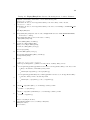
I believe the non-anticipated case which was briefly described in the draft holds
more promise for a simple and still effective mechanism at reducing packet loss and
reducing handover latency without the coupling to specific L2 technologies required
by the anticipated case discussed above. Non-anticipated fast handovers do not
require knowledge of which AR will be the NAR. There is no exchange of PrRtAdv
or RtSolPr at PAR’s link as shown in Figure 3.3. In fact the Handover Initiation
phase does not occur at all. The MN upon attaching to new link (NAR’s link) as
indicated by reception of a L2 “link up” trigger will send a RS with FNA. This is
required to learn the default router’s i.e. NAR’s IP and link layer address. Then
send a FBU to the PAR using its CoA (PCoA) as source address. The NAR if
it supports FMIP has to allow in its ingress filtering rules any packets destined to
PAR with a source address belonging to PAR’s subnet, in this case PCoA fulfils
this criteria as it has been autoconfigured via the address configuration mechanism
described in Section 2.2.1.2. Once FBU reaches PAR, the PAR will quickly do the
HI and HACK exchange to complete the tunnel establishment stage. The NAR
in my opinion should not need to verify the NCoA’s uniqueness nor defend it. In
fact it should leave all NCoA configuration to the MN because there is now no
advantage in having it done by NAR unless stateful address configuration is used.
In the meantime the MN can use the PCoA as if it still existed on the old link as a
bidirectional tunnel should have been established between PAR and NAR by then.
Reception of a BACK from the PAR is confirmation of tunnel establishment. If we
29
take the view that the wireless link delay is much greater than the delay existing on
the link between PAR and NAR then packet loss should be minimised. The MN is
also free to simultaneously configure NCoA as done in MIPv6 as soon as it receives
the RA that should include a NAACK indicating that NCoA is invalid to force MN
to do address configuration as described in Section 2.2.1.2.
Figure 3.3: Non-anticipated Fast Handover Operation
The non-anticipated case while not able to reduce the rendezvous time to zero
as the anticipated case promises to, it can reduce the overall handover latency as
packets are forwarded quickly from the PAR to the NAR and allows the MN to
resume communication via the PAR to NAR tunnel without waiting for registration
with HA to complete as base MIPv6 would require. It buys the MN additional time
to perform DAD and binding updates without interrupting communications.
30
3.2
Layer Two “Link Up” Trigger
In reactive handovers as mentioned at Chapter 3 there is a delay at the MN associated
with recognising a new Layer 3 or Network Layer (L3) point of attachment called the
rendezvous time. The previous section mentioned the use of the full complement of
L2 triggers to implement FMIP. Since this would require some modification of existing
L2 technology it would be a rather expensive exercise. The link up trigger (L2 Trigger)
that is commonly implemented in virtually all wired and wireless devices is the “link
up” trigger which from now on will simply be referred to as L2 Trigger.
This simple notification from L2 can help to reduce rendezvous time because
it detects a change in the L2 link. Whilst it is possible that a L2 handover is not
associated with an L3 handover this mis-prediction will have cost only a RS and the
corresponding RA to tell the MN it had not changed L3 point of attachment and so
should not initiate L3 handover. So the benefits for L2 Trigger should outweigh by far
the cost except in situations where there are frequent L2 handovers or moving in and
out of range of a solo coverage range so that large numbers of MNs performing router
discovery could take up considerable bandwidth. This is not really too much of an
issue in deployment because if the MN is residing at the periphery of the coverage
range then the coverage range should be extended by adding extra APs or the MN
has to restrict its mobility within the existing coverage range.
3.3
Fast Solicited Router Advertisements
During router discovery, when a mobile node sends a RS and awaits the RA from the
local subnet router, there is a random amount of time6 before the RA is sent back in
response as specified in RFC 2461 [34]. This is so that Router Advertisements on the
local subnet are desynchronised in cases where more than one router exists to prevent
flooding of the network and collisions on common broadcast media like Ethernet.
6
0 to MAX RA DELAY TIME (500ms default)
31
This is where an amendment to RFC2461 called Fast Router Advertisements7 [38]
can help. It is especially tailored for ARs that will have MNs visiting their links, as
an expeditious solicited RA can reduce the rendezvous delay and hence the overall
handover latency. This is achieved by choosing one router on the link to serve as the
“fast RA” router. Only that designated router is allowed to respond immediately
with a unicast RA to a mobile node that sends a RS with a proper8 source address.
There is an allowance for fast RAs up to a configurable maximum of FastRACounter
that is 10 by default. Any more RSs beyond that will be scheduled for a normal
unsolicited multicast RA as described in RFC 2461.
3.4
Optimistic Duplicate Address Detection
Optimistic DAD [39] is an Internet draft describing a method of allowing a node to
use a tentative address i.e. an address undergoing DAD as source address which is
contrary to the standard behaviour defined in [34]. It operates under the assumption
that the addresses chosen for DAD on a particular link layer technology are well distributed so as to minimise the chance of duplicate addresses. This is certainly true of
Ethernet based technologies such as IEEE 802.11b. Nodes implementing Optimistic
Duplicate Address Detection (ODAD) will be able to resume communications much
earlier after a handover by carrying out standard DAD in parallel.
ODAD enforces certain restrictions on what can be done with the tentative
address so that disruption to the legitimate node who actually owns the tentative
address will be minimal. This guarantee is enforced by the following:
• Router solicitations do not include a source link-layer address when sent from a
tentative address. This ensures that the router will not associate the tentative
address with the optimistic node and redirect any possible ongoing communi7
Hereinafter referred to as Fast Solicited Router Advertisement (FSRA) in this thesis to avoid
confusion with fast RA beacons which are unsolicited RAs.
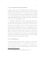
8
Any valid address besides the unspecified address.
32
cation sessions by the legitimate node to the optimistic node.
• The node forwards any packets to neighbours via the router. So only the router
is aware of the node’s presence on the link.
• Override flag is never set in neighbour advertisements. This will prevent the
neighbouring nodes’ neighbour cache entries of a legitimate node from been
overwritten by the erroneous duplicate address of the optimistic node. This
ensures ongoing communication sessions by the legitimate node with neighbours are never disturbed. This also allows the legitimate node to defend its
address by sending a neigbhour advertisement (NA) with the override bit set
to ensure the optimistic node knows that it has a duplicate address tentatively
assigned and will stop using it.
There is also a procedure to generate a new random suffix and hence form
another IP address to undergo DAD. This is a simple method to automatically recover from duplicate addresses since the standard behaviour in IPv6 calls for manual
intervention.
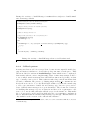
3.5
Previous Care of Address Forwarding
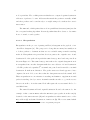
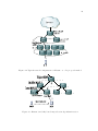
Previous care-of address Forwarding was described in earlier revisions of the MIPv6
Internet draft9 . It was removed due to security considerations10 . Previous care-of
address Forwarding (PCoAF) is the MIPv6 equivalent of smooth handover from MIP.
PCoAF uses only stock MIPv6 functionality. The MN regards the previous access
link as its “home subnet” and sends a BU to PAR with the HoA set to the PCoA and
the CoA to the NCoA as shown in Figure 3.4. Messages destined for the MN at PCoA
will be intercepted, encapsulated and forwarded by PAR to the MN at its NCoA.
9
see Section 11.6.6 of http://www.watersprings.org/pub/id/draft-ietf-mobileip-ipv6-18.txt
basically a security association would need to exist between the PAR and the MN similar to the
one that exists between the HA and the MN
10
33
PCoAF mitigates the effects of a topologically distant HA or CN by using the
PAR to forward the packets addressed to the PCoA while the BU is sent to the HA
and CN. This ensures a minimal number of lost packets when the traffic type is of
the multimedia variety and the MN seldom acknowledges received packets i.e large
synchronisation buffer so that the MN does not need to acknowledge packets during
the handover in order to continue receiving packets.
HA
CN
CN
foreign subnet
HA
PAR
HA
NAR
Movement
MN
Figure 3.4: Previous care-of address Forwarding in action
This is also functionally similar to the non-anticipated fast handovers discussed
previously at Section 3.1 in terms of been able to reduce the number of dropped
packets after handover. Whilst non-anticipated fast handovers may have the upper
hand by allowing the MN to resume communications using its PCoA as soon as
it has detected movement to NAR and thus a greater reduction in the number of
dropped packets, this comes at a cost of adding fast handover functionality at the
edge of the network which is not a trivial task11 , and an additional overhead of
signalling messages between PAR and NAR. All PCoAF requires is that all ARs have
11
see [40] for the mathematical analysis of timing the tunnel establishment for optimal FMIP
handover to prevent excessive overhead in signalling and buffering
34
HA functionality. However with the addition of ODAD, and Fast Solicited Router
Advertisement (FSRA) this mechanism is at least as fast as non-anticipated fast
handovers and can come close to the anticipated version. Close only because in
anticipated mode of fast handovers the task of establishing a forwarding tunnel is
accomplished just before handover whilst in the combined version of PCoAF there
will still be some delay in configuring a CoA on new link and sending a BU to PCoA.
While these AR local extensions can improve handover times, they still can
not solve the problem of excessive signalling that occurs when the MN moves frequently within a small geographical area while away from home. When the MN
moves just beyond limit of link layer connectivity to its previous subnet, it needs
to send a BU all the way to the HA even when it may be moving back soon into
the previous cell’s coverage range. MIPv6 was not designed with this in mind since
its sole purpose was to allow Internet access on the move albeit not seamlessly and
efficiently though. These shortcomings led to the development of localised mobility
management protocols which are the subject of the next chapter.
Chapter 4
Localised Mobility Management
Wireless Internet is expected to surpass traditional methods of access1 in the near
future [41]. Table 4.1 depicts the general trend in the declining cost of wireless Internet access. Currently ubiquitous wireless Internet access via Wireless Local Area
Network (WLAN) is not available yet due to the ten challenges identified by Ritter
in [6]. One of them is fast handovers. MIPv6 handovers are subjected to variable
delays as the signalling between the MN and the correspondent entities2 introduce
varying latencies that magnify the bursty ’packet-switched’ nature of the Internet
where network applications are already subjected to non-deterministic delays arising
from congestion. Real time protocols demand stringent bounds on delay for packet
delivery [41], otherwise noticeable degradation in quality occurs. As the MN moves
over different provider networks as shown in Figure 4.1, it signals the HA and CN as
a result of new points of attachment to the Internet. Eventually the round trip time
of the BU and Binding Acknowledgement (BA) exchange will exceed the bounds on
delay imposed by real time traffic and loss of quality is perceived by the end user.
This effect is much more pronounced as the MN increases its mobility, triggering
more handovers and causing more packet loss due to delayed delivery of packets to
1
2
Ethernet, Digital Subscriber Line (DSL) and cable
CN and HA
35
36
real-time applications3 .
Technology
Data Rate(kbps)
$/kbps
GPRS
53
$118.91
1xRTT
153
$25.42
Richochet
248
$2.43
WLAN
5500
$0.27
iBurst
1000
$0.25
Table 4.1: Cost (USD) of a standardised plan per available user
bandwidth (in kbps) for different wireless access technologies. All
data was from [6] except iBurst. IBurst estimate from Veritel at
http://www.veritel.com.au/FreedomPricingandPlans.html assuming 12 months inc. purchase of card and not exceeding monthly
download limit of 500MB
LMM4 is the generic term for IP Mobility Management (MM) protocols that aim
to minimise the excessive signalling (BUs) to its peers caused by frequent change of
CoA. This is achieved by confining the mobility signalling within an administrative
domain. A Localised Mobility Agent (LMA) is introduced into the visited domain
in order to reduce the excessive round trip times that would otherwise result from
registering with the HA. This is a relatively new research area as there have not
been any large deployments of Mobile IP [8] and Mobile IPv6 is still in draft status.
The general mechanism of LMM can be seen in Figure 4.2 where an MN is initially moving away from its home domain into the visited domain. This is known as
an inter-domain transition because the MN moves between different administrative
regions. A home registration is sent to the HA and is classified as a global mobility
3
these applications only accept packets that are within the bounds of delay as required by the
audio and/or video codec and discard packets that do not satisfy this constraint
4
micromobility is a subset of LMM generally denoting use over a small geographical area
37
Figure 4.1: MN movement between networks in the global Internet requires mobility
bindings to be updated with peers. (Reproduced from [41])
signal. Because the BUs are sent to the true peer entities (CNs and HA) and propagate across different administrative regions. This is the exactly the functionality
that MIPv6 provides.
Inside the visited domain, the MN moves from one subnet to another and these
are called intra-domain transitions. An intra-domain transition involves the exchange of localised or regional mobility signals with the LMA and so are confined
within a single administrative region. This BU is also known as a Regional Binding
Update (RBU). The LMA is thus responsible for maintaining a forwarding or look
up table that maps the MN’s regional care-of address (RCoA) known by the HA
and potentially CNs from the global mobility signals sent by the MN, to the current
location of the MN i.e. local care-of address (LCoA) within the visited domain that
the regional mobility signals provide. In effect it is acting as a local HA within this
foreign domain. LMM implies not changing the address the HA and CNs use to
reach the MN for any host movement within the visited domain. By moving the
MM to the LMA so that it is closer to the MN, the MM process is dictated by the
38
topological size of the administrative domain as opposed to the variable number of
hops(represented as backbone round trip time in Figure 4.2 ) between the HA and
MN across the wide expanse of the Internet. The indirection provided by the LMA
is supported by empirical evidence from Kirby [42] that 68% of an MN’s movement
occurs within a local region. LMM alone does not guarantee the end-to-end delay
constraints of real time traffic are satisfied. However I believe it is a prerequisite for
reaching the goal of seamless mobility across the Internet.
Figure 4.2: Introduction of LMA for MM reduces the number of mobility bindings to
the HA when mobility is restricted to the foreign domain. (Reproduced from [41])
There have been attempts to extend MIPv6 or proposals of new MM protocols
that can be used for both intra-domain as well as inter-domain mobility. However
it makes sense to separate the two mobility functions due to the following benefits
[43]:
• Allows independent evolution of LMM protocols and base IP mobility provided by MIPv6
• There is no difference between wired or wireless access networks to the core IP
39
network, because MIPv6 is the common mobility protocol used between access
networks.
• Allows for different LMM solutions to cater for the different access network
technologies
• Allows access network providers to use an LMM solution that suit their needs
best [44]
• Does not prevent introduction of new protocols in the access network
• Confines intra-domain mobility signalling to access networks instead of dispersing throughout the core of the Internet on each L3 handover.
There have been many LMM proposals suggested in light of the fact that MIPv6
has not been deployed commercially yet. In order to evaluate these Pagtzis et. el.
have formally submitted an IETF draft on Local Mobility Management Requirements
earlier this year and elaborated on the requirements in [41]. The major requirements
of interest are:
• robust so that no single points of failure or routing loops occur
• minimise the effect of triangular routing that is caused by introducing LMM
• no additional functionality required over base MIPv6
• incremental deployment
• no increase in signalling messages to HA and CNs over base MIPv6
• no increase in latency, packet loss, service disruption over base MIPv6
• LMM complexity scales at most linearly with size of domain and MN number
• Resilience to topological change
• minimal manual configuration
40
• no disruption to core IP routing outside of an administrative domain
Traditionally LMM protocols have been categorised as tunnelling or routing
schemes [8, 44]. The routing schemes use conventional IP routing for redirection of
the MN’s CoA to its current location. The lookup tables are distributed amongst
all mobility agents in the management domain. Examples of routing schemes are
Handoff-Aware Wireless Access Internet Infrastructure (HAWAII) and Cellular IP.
Tunnel-based schemes use LMAs for registration and tunnel packets to the MN
with few agents having knowledge of the node’s location. HMIPv6 and regional
registration extension for MIP are examples of tunnel based schemes. Chiussi et. el.
argue that routing based schemes such as Cellular IP have poor scaling properties
as all nodes are required to establish forwarding tables to the MN on the up-link
path and are not conducive to incremental deployment because all routers require
this functionality.
Eardley et. el. disagree with this traditional classification as it does not in
their view offer any useful information on the performance of the protocol [44]. In
their view these protocols should be classified based on their scalability, in particular
terminal scalability, throughput scalability and geographical scalability. They state
that terminal scalability is the ability for many wireless devices (potentially in the
millions) to be accessible in the one access network (AN) is really just a problem
of addressing. Given a proper address allocation procedure they do not think this
should be a problem. In their opinion this excludes auto configuration as the MN
has no way of knowing which addresses are already in use. Geographic scalability is
the ability to service small home networks all the way up to a global network and
throughput scalability would require flexible network topologies with many access
network gateways (ANG) as shown in Figure 4.3. Support for arbitrary topologies
allows operators the freedom to deploy the network with the required resilience allowing multiple paths to avoid congestion. Multiple access network gateway (ANG)s
are necessary for throughput scalability and robustness. They state that seamless
41
handovers5 (handover management) does not need to be scalable. I disagree as the
future of wireless Internet will most certainly be a multimedia rich experience so the
signalling to local ARs to effect fast handovers will be crucial and dare I say all MNs
will need this although perhaps not all the time and not altogether at once.
Figure 4.3: Conceptual AN architecture
They agree with Chiussi et. el. when it comes to criticising Cellular IP for been
unscalable since the packets always travel the same path due to the strict hierarchy,
so there is no provision for multiple ANGs. The surprising thing is that they also say
that HMIPv6 if used in a hierarchical fashion will be no different from a performance
point of view. The example used of mobile to mobile communication in the same
access domain that can be very large, in the worst case may need to be established
via the ANG is simply incorrect because in HMIPv6 route optimisation can be used to
have the two nodes communicating directly rather than via the LMA if privacy is of
no importance. So there should not be a need for a hierarchy of MAP registrations.
This is also stated in the HMIPv6 draft [45, 20] too, where it is acknowledged a
hierarchy of map bindings would degrade performance.
5
minimising packet loss and delay
42
4.1
Hierarchical Mobile IPv6
HMIPv6 is simple in concept because it literally places the role of the HA into the
LMA and referred to as a MAP [45]. The intra-domain transitions are defined as
movements within the MAP domain. A MAP domain is delineated by the ARs
that forward the same MAP option inside a router advertisement. The MN detects
the presence of a MAP from the RA’s MAP options. The MN chooses the best
map according to its own policy6 if there were more than one and perform global
registrations for the first time only to the CNs and HA. While it continues to detect
the same MAP option at every handover it will only need to send a regional update
that is a BU to the MAP. If it does not detect the same MAP but another MAP is
advertised it can bind with the new one. If no other MAPs are advertised then it
reverts back to MIPv6. Either way whenever the MN leaves a MAP domain it will
have to update the global mobility bindings.
The following is a list of advantages in deploying HMIPv6 as an LMM solution
[45].
• Reduces the number of global registrations to the HA and CNs
• Actual reduction in number of messages over the wireless interface because
only the MAP is updated with new mobility binding and not every CN for
every MN transition within the MAP domain.
• Reduces handover latency because the return routability procedure of MIPv6
is required for every CN registration. As explained before this is at a minimum
one and a half round trips. By binding to the MAP this eliminates the need
to do CN registration.
• Only one binding update is required at the MAP before all traffic from CNs
6
HMIPv6 draft recommends using a furthest MAP policy. This favours a mobile node that moves
frequently so the number of bindings to the HA are reduced, since a further MAP’s domain consists
of more ARs. The down side is intra-domain handovers take longer.
43
and the HA are redirected to its new location.
• Those with privacy concerns can always use the RCoA as source address option
when communicating with the CN so that route optimisation is on only at the
global level7 , so the CN cannot track the movement of the MN within the MAP
domain.
• Easy to deploy as no changes are required at the HA and the CNs
• Allows ingress filtering rules at ARs to remain unchanged in the MAP domain
as the MAP supports reverse tunnelling from the MN. However this adds extra
overhead.
While the advantages are numerous there are also many disadvantages. The
major ones would have to be the non-optimal routing, MAP discovery mechanism
and recovery from MAP failures and poor MAP selection algorithm. The non-optimal
routing forces a single point of failure and so does not satisfy the geographic scalability requirement discussed in Chapter 4. The default MAP selection procedure
will select the same MAP for all MNs at ARs that are the same distance from the
farthest MAP which would be the MAPs at or close to the gateways of an administrative domain. Thus the MAP will be a bottleneck. The HMIPv6 draft notes
that the use of the preference value may be able to control this to some degree, so
for overloaded MAPs they decrease their preference value. However this will simply
move the problem to another MAP and becomes the classic routing problem of flutter
where the congestion hotspot just moves around. There needs to be a domain wide
load balancing scheme so that the MAP boundaries for each MAP can be adjusted
at the same time as their preference values and in coordination with other MAPs.
MAP discovery by default is a manual process because the MAPs and ARs
have to be configured before deployment. The configuration involves enabling which
interface in the MAP and/or AR should send or forward the MAP option on, and
7
the truly paranoid can turn off route optimisation altogether by sacrificing efficiency
44
hence control the size of the MAP domain. For large administrative networks this
involve a lot of manual work. While there exists an automatic method to propagate
the boundaries of the MAP domain so routers know which interface to forward MAP
options on [45, 17], the actual determination of the MAP boundary remains a manual
process.
Can be very high in overhead with up to two sets of tunnel headers in both
directions if the following conditions are met.
1. The MN cannot perform route optimisation with the CN since according to the
HMIPv6 draft, MIPv6 does not mandate that all CNs be able to cache mobile
bindings. So standard MIPv6 reverse tunnelling comes into play with tunnel
entry point of RCoA and exit point of the HA’s global address.
2. Alternatively the MN may not want the CN to even know its RCoA for privacy
reasons and so the previous behaviour applies
3. Most ARs perform ingress filtering by default to prevent masquerade8 so the
MN will have to use reverse tunnelling with local care-of address (LCoA) as
tunnel entry and the MAP’s global address as tunnel exit. Either that or the
network administrators will have to reconfigure all their ARs taking care to
just allow the prefix for forming RCoA addresses through the ingress filtering
rules. Thus reverse tunnelling is an advantage too, since it allows HMIPv6 to
be deployed without configuration of AR ingress filtering rules.
There will always be one tunnel since the MAP has to keep the original packet
intact and so a tunnel from the MAP to MN exists with tunnel entry of MAP’s global
address and exit point of MN’s LCoA. While it is possible to eliminate even this
tunnel by route optimising all the way to the MN, so the CN knows about the LCoA
too, this defeats the purpose of HMIPv6. This mode of communication is only valid
8
Malicious nodes can use any source address and a non-ingress filtering router will forward them
even when they are not topologically correct
45
for very brief communication sessions where the MN is not likely to handover yet.
The MAP selection algorithm also needs to be much more adaptable than just
a choose the farthest MAP algorithm. Further work has been proposed in this area
and is presented in Section 4.3.
4.2
Fast Handovers in HMIPv6
Fast Handovers in HMIPv6 [46] aims to combine both HMIPv6 and FMIP to gain
the benefit of HMIPv6’s reduced signalling and registration times as well as shorter
rendezvous time that FMIP buys. The argument goes that simply integrating the
two protocols does not always reap the maximum benefit because:
1. increased tunnelling overhead
2. increased processing time at routers to process extra tunnel headers
3. the path that packets traverse may be such that the MAP is between the NAR
and the PAR and the CN is closer to the NAR. Using this naive approach would
mean that packets traverse an extra round trip back to the PAR for no reason
at all
To overcome these problems they proposed to replace the PAR with MAP. They
say that their solution cannot work with non anticipated fast handover. However
I say that it is possible if you set up the ingress filtering rule at NAR with all the
MAPs in the domain instead of just the neighbouring PARs. This requires more
coordination but certainly not as much as when compared to the amount of L2
support and coordination between APs and ARs required by anticipated handovers.
46
4.3
Local Mobility Agent Selection Algorithms
For micromobility it is very important how the MAP is chosen as it determines
the latency and frequency of inter-domain handovers. This in turn depends on the
mobility of the MN. HMIPv6 allows nodes to select the MAPs themselves. This is a
two edged sword, because on the one hand, the MN knows what its requirements are
so it can select the best MAP from its perspective. On the other hand any global
scheme that tries to enforce which set of MNs are served by which MAPs have a hard
time of enforcing this, since the MN is allowed to register with any MAP. While the
MAP is at liberty to reject any BUs, this trial and error process will take a while
before the MN has bound with the “preferred” MAP especially when many MAPs are
available for popular sites.
Hop-by-Hop-Based LMA selection proposed in [47] has better MAP discovery
mechanism than HMIPv6 because it actually involves a form of pinging to discover
the LMAs rather than requiring ARs to forward them. But it still finds the farthest
MAP so assuming high mobility in visited domain just like HMIPv6. Their protocol
satisfied all the LMM requirements [48] mentioned in [41]. The explanation of the
recovery mechanism was rather brief no more than a sentence in each reference and
was to the effect of using source routing to see if it can still get a probe response
from the registered (furthest LMA). If it does not then it should use the stored
responses to choose the next furthest to register with. If all that fails then restart
probe discovery. This mechanism is slow if inter-domain transitions are frequent
as it backtracks through the list of LMAs in previously visited domains. The RFC
has expired as of June 2003 so perhaps the authors do not think it is worthwhile in
pursuing further.
The same group has proposed another LMM solution called Mobile Controlled
Movement Tracking LMA Selection [49, 50]. It is similar in strategy to the MPLSbased mobility [8] because it also selects a close (in terms of number of hops) LMA
47
to reduce signalling delay and yet far enough to cover the movement of the MN to
reduce frequency of global handovers.
As mentioned before the rate of mobility is an important factor when deciding
which MAP to register with. Kawano et. el. in [51] have taken this one step
further and created a MAP selection algorithm that classifies the node’s mobility
based on its dwell time in a MAP domain and chooses a MAP to match9 . In their
performance evaluation of their proposed method for the network configuration as
shown in Figure 4.4, there are only 2 types of nodes fast and slow. The threshold
at which a MN is considered fast is 20km/h for their experiment. The MN does not
choose the MAP but rather UA (User Agent) situated at the access router (AR) as
shown in Figure 4.5. Whenever a node sends a BU it is the AR that intercepts this
BU and the UA is instantiated to look at the Selection Table (ST).
The ST contains some simple entries that determine which MAP to register
with for that particular speed profile. The ST’s are most likely precomputed and
placed in each AR in such a manner as to effect a distributed and equal load across all
MAPs in the administrative domain. The AR then sends a BU to the corresponding
MAP on behalf of the MN. The details of who the BU was originally addressed to
and the mechanism of proxy BU requests are not stated in the article.
Their simulation experiment was conducted in a network with a hierarchy of
an m-ary tree. i.e. 1x16x16x4 (The root or core router of the domain was connected to the sixteen MAPs designated simply as higher MAPs and each higher
MAP had 16 MAPs below them designated as lower MAPs and each lower MAP
had 4 ARs). The output parameters used to judge performance were the number of
BUs and also the mean number of MNs managed per MAP. They compared their
method against three schemes; one that always chose the higher MAP; one that
always chose the lower MAP; a random MAP. Their method consistently performed
better than the other three schemes where relevant and they also proved that their
9
for details of the algorithm please consult [51]
48
Figure 4.4: Typical network configuration for Kawano et. el.’s proposed method
Figure 4.5: Kawano’s mobility based map selection algorithm in action
49
protocol is independent of the network topology to some extent as they tried it on
a different topology (1x4x16x16 m-ary tree) too. Most importantly they varied the
actual threshold parameter from 0 to 50 km/hr in increments of 10 and were able to
show that for threshold settings above 10km/hr their method also outperformed the
other three. Thus the speed threshold need not be accurate just a reasonable enough
estimate, since the algorithm is robust enough to tolerate a wide error margin. The
only problems with these results are that they gave no mention of the simulation
model used. The protocol at face value looks like it has some merit however there
will usually be more than two levels of hierarchy in large 3G networks so it would be
interesting to test if it could handle say up to six or seven hierarchies. Another difficult problem would be the creation and distribution of these ST tables as manually
pre-computing them and distributing is not scalable for large access networks. The
only feasible alternative is for extra signalling to be introduced to exchange the load
information on each MAP and calculate the ST separately at each UA at regular
intervals.
4.4
Other Micromobility Protocols
Cellular IP and HAWAII have both been mentioned previously. Cellular IP is a
mechanism that modifies base IPv6 forwarding in such a way so as to allow upstream
data packets sent by the MNs to create forwarding entries in the opposite direction.
This in effect is very similar to the way Ethernet switches work. The MNs register
the ANG’s address as their CoA. The downstream packets which will be extracted by
the ANG and have the HoA as source and flow through the modified routers and use
these recorded routes in reverse to reach the MN’s current location. Thus the whole
access network becomes a flat host based routing scheme and so is not considered
scalable by many.
Kim and Song in [52] suggest using a periodic binding update method to reduce
50
the number of unnecessary binding updates and hence reduce signalling load on
network and processing delay for handover when a node is highly mobile10 or moves
back and forth frequently between a few links. Their method works by choosing
a value for the configurable time period t based on the mobility of the node. At
every t seconds the node will detect if the current network prefix as advertised by
the router is different from its care of address. Only if it is different will it perform
a layer 3 handover and send a binding update to the HA and CN. Otherwise it
will reset the timer. The routers on the foreign links will have to be able to buffer
the packets whilst the MN moves to different foreign link without notifying CN and
HA. After MN registers new location with CN and/or HA then it is able to request
previous foreign link to forward buffered packets to itself as shown in Figure 4.6.
Their M/M/n queueing analysis found that as long as the probability of binding
at every t seconds is less than 70% then there is an improvement in the processing
delay as compared to plain MIPv6.
Figure 4.6: Time-based binding update in action
In [9] the authors claim that their proposed protocol Cellular Mobile IPv6
(CMIPv6) can reduce L3 handover by using foreign home agent (FHA)s11 to track
location of the MN that according to the authors is better than HMIPv6 for cellular
networks. The FHA appears to spy on the link for BUs and will store some location
information into a Location Table (LT). When the MN moves and sends a BU to its
peers, the FHA is able to determine the NCoA of the MN from the BU that passes
10
11
approx. 112km/hr in their analysis
a modified router
51
through it to the peer node. Thus it is able to set a temporary forwarding from
the PCoA to the NCoA for any packets in transit before the BU arrives at the MN’s
peers. This is similar to Cellular IP except this modifies normal packet processing
during handover only. It does improve handover latency over MIPv6. CMIPv6 is
most effective when the rendezvous time is small in comparison to registration time
as communications resumes just after the BU is sent. Their evidence for this is
that the Linux MIPv6 implementation takes only 200ms for acquiring a CoA. This
is an exaggeration because it does not seem to take DAD into account, unless their
link-layer technology does not require DAD.
There are also LMM schemes that borrow successful protocols from different domains such as Multi Protocol Label Switching (MPLS) from Traffic Engineering (TE)
[8] and a multicast-based one called Multicast-based Micro Mobility [53]. Basically
both of these protocols borrow from the signalling primitives already available and
which have proven to be effective for their application areas. For MPLS the argument is that MPLS is actually more efficient than IP itself since MPLS labels are
used for forwarding purposes. It should be more scalable since MPLS can handle
thousands of labelled paths and has proved more than capable. For the multicastbased method their argument was that the multicast tree is perfect for forwarding
to the MN’s current location. The route will always be route optimised since that
is a property of the multicast algorithm. It uses multicast group joins and leaves to
notify the network of where the MN is exactly. Thus it is rather similar to Cellular
IP in that the routing information is distributed in many nodes but this is much
more efficient because the author has used some kind of algorithm to aggregate the
state information so that it occupies less memory.
Chapter 5
Performance Evaluation of
Mobile IPv6 Enhancements
5.1
IPv6Suite Simulation Framework
In order to carry out the performance evaluation of MIPv6 and its extensions, I have
chosen to use simulation as the tool instead of mathematical analysis. Simulation is
a valid tool for determining the performance of communication protocols especially
when mathematical models are too complex [54] or intractable. Many of the communication protocols involved in large networks are very detailed and can give rise
to complex behaviour i.e. extra retransmission of some protocols may increase overhead many times. We1 have constructed an IPv6 simulation suite called IPv6Suite
[55] released under the GPL2 . IPv6Suite was initially based on IPSuite3 . It is now
significantly improved and adds the following protocols:
• RFC 2373 IP Version 6 Addressing Architecture [31]
• RFC 2460 Internet Protocol, Version 6 (IPv6) Specification [13]
1
Eric Wu and I
http://ctieware.eng.monash.edu.au/twiki/bin/view/Simulation/IPv6Suite
3
IPSuite is an IPv4 network simulation suite [56]
2
52
53
• RFC 2461 Neighbour Discovery for IP Version 6 (IPv6) [34]
• RFC 2462 IPv6 Stateless Address Autoconfiguration [30]
• RFC 2463 Internet Control Message Protocol (ICMPv6) for the Internet Protocol Version 6 (IPv6) Specification [57]
• RFC 2472 IP Version 6 over PPP [58]
• RFC 2473 Generic Packet Tunneling in IPv6 [33]
• Mobility Support in IPv6 (MIPv6) revision 184
• RFC 2464 Transmission of IPv6 Packets over Ethernet Networks
• RFC 2374 An IPv6 Aggregatable Global Unicast Address Format
• Hierarchical Mobile IPv6 Mobility Management (HMIPv6) revision 6 [45]
• Optimistic Duplicate Address Detection [39]
• Fast Solicited Router Advertisements revision 4 [38]
IPv6Suite is built on top of Objective Modular Network Testbed in C++ (OMNeT++). OMNeT++ [59, 60] is a discrete event simulation platform written using
C++ [61]. Here are some of the features from OMNeT++ that I find compelling:
* Many models are available including IPSuite [56].
* Scalable compared to other simulation systems see Appendix A and B of [60].
* Unlimited5 levels of granularity via the compound/simple module approach.
* Object oriented paradigm
* Well documented
4
5
Without the Return Routability procedure
restricted by the amount of computing resources at your disposal
54
* Author is very helpful and friendly
* Open Source and free for academic research
The goal of the IPv6Suite is to be as accurate as possible without sacrificing performance and scalability. It needed to be scalable because we plan to use
IPv6Suite as a platform to simulate realistic and very large scale networks in order
to understand how well new proposals such as MIPv6 perform when tested in network configurations larger than the size of laboratory testbeds. Please refer to our
paper [62] where details of the modifications to OMNeT++ for parallel simulation on
computing clusters are explained. A hands on tutorial for a basic parallel simulation
is provided in [63]. For an introductory overview of IPv6Suite please refer to our
paper [55]. For a detailed design of IPv6Suite please turn to Appendix A.
5.2
IPv6Suite Deviations from MIPv6 IETF draft
Eric Wu and I have implemented draft 15 of MIPv6 with some updates and clarifications from draft 18 too. However the major omission of draft 18 would be the
missing return routability procedure that adds an extra round trip and a half. It is
a prerequisite before sending bindings to CNs as explained in Section 2.2.2.2.
Neighbour Unreachability Detection is another method of detecting MN movement which is not implemented in our simulation. This is no loss because the Mobile
IPv6 for Linux (MIPL) implementation does not use Neighbour Unreachability Detection (NUD) either [36] because NUD is one of the slower forms of movement
detection mechanisms. NUD is started when a different network prefix is advertised
by a new AR to ensure that the HA or PAR is not reachable on the local network
anymore since it is possible for a link to have two ARs advertising different prefixes.
Our MIPv6 implementation undergoes DAD on the acquisition of a new CoA
only. DAD is not done for the link local address upon visiting a foreign subnet as
55
RFC 2462 states that stateless autoconfigured link local addresses need to have DAD
done once only. However the latest revision6 of MIPv6 draft has stated that DAD
SHOULD be done upon visiting a new foreign link7 . Most simulations do not even
consider the effect of DAD. A case in point is Figure 10 of [9] that shows a value of
200ms for acquiring a new CoA that is well below the requirement of awaiting DAD
completion that should be at least RETRANS TIMER8 seconds.
MIPv6 stipulates that the first home registration to HA should wait for BA before
signalling the CN. However in draft 24 there is also one sentence that reads as always
wait for the BA from HA before sending BU to CN. I believe this interpretation to
be correct because return routability depends on the registrations to the HA and CN
occurring in sequential order. This is so that the HA knows the MN’s current location
(CoA) before return routability can succeed and hence a successful registration at
the CN. In my MIPv6 model there is no delay before registering with the CN as that
is done immediately after sending BU to HA. I do not see any problems with this
because the packets sent by CN to MN in the route optimised mode of communication
bypasses the HA. However return routability will not allow this optimisation so the
simulation results are somewhat optimistic about the handover performance for all
the mobility management protocols tested.
The HA should perform DAD on behalf of the MN for the HoA at the first
binding. This is to ensure that no other node has acquired HoA during the window
of opportunity available when the MN moves away from its home subnet and before
the HA starts defending the HoA. This will introduce a significant delay during the
first handoff only. ODAD cannot be used here since the purpose of a HoA is a
permanent identifier like a phone number for the MN, generating another HoA is not
acceptable. A foolproof solution to this is to use some form of stateful configuration
like Dynamic Host Configuration Protocol for IPv6 (DHCPv6) at the home subnet
6
24 at the time of writing
see Section 3.4 of [39] for an explanation on why
8
one by default
7
56
to ensure that the HoA is not assigned to another node even though the chances
of autoconfiguring the same HoA are slim. This initial DAD on HoA by the HA
is not done in the simulation because we can assume that if users want seamless
handovers during the first handoff, they would have to use DHCPv6 or reduce the
RETRANS TIMER value or just turn off DAD9 at the home subnet. The DAD
approach is always a trade off between convenience and the chance that two nodes
share the same address. DAD completion does not guarantee that the address is
unique only the chance of a duplicate address has reduced. The default value for
DAD is just one neighbour solicitation [30] and so on the lossy wireless links is prone
to be lost.
In light of the extra delay caused by return routability that are missing from
the simulation model, the simulation model is not an exact representation of the
current state of the MIPv6 proposal at revision 24. These results are much more
optimistic and the introduction of these delays would cause some forms of real time
streaming that require stringent and very low delays to lose synchronisation during
handover and render some of the more fragile voice and/or video codecs unusable or
at least perform poorly when the MN transitions frequently.
5.3
Simulation Scenarios
Each simulation experiment is conducted with the input parameters set as stated in
the text using the methods described in Appendix B.
The determination for the number of simulation runs (replications) for each
experiment initially used Akaroa [64] to record the number of observations i.e. handovers to achieve a certain level of statistical confidence.However due to a technical
problem, the observations were not recorded by the Akaroa library so a manual
method was used instead. Based on the objective of 95% confidence level10 and
9
10
by setting host duplicate address retransmits variable to zero
95% of the time, conducting this experiment will produce confidence interval limits that bound
57
an approximate precision of ±50ms I have determined that 100 runs were sufficient
(assuming there were 4 handovers per run) based on preliminary trials. It is not possible a priori to establish the number of runs for a required confidence interval (CI)
because the standard deviation σ is unknown as shown in Equation (5.1) [65].
n=
z
a/2 σ
E
2
=
1.96σ
0.05
2
(5.1)
All results have been tabulated with the number of handovers used and the
calculation for the confidence interval limits for a 95% confidence level by Equation (5.2)
za/2 σ
x± √
n
(5.2)
where x is the sample mean and za/2 for a normal distribution is approximately 1.96.
The actual calculations used the Student-t distribution.
The links and their link delays in each scenario described below can be considered as an abstract and simplified version of the Internet with constant delay even
though the simulation has modelled the path between the CN, the AR and the HA
as a single link. The link delays in the scenario are are actually propagation delays
in the simulation. However, they should be considered as a delay experienced by
a packet travelling that path. This simple model should give results that are adequate in comparing the relative benefits of each scheme. For accurate depictions
of the absolute handover latencies and packet loss, a large scale network topology
representing the Internet is required at the expense of longer simulation times and
complex modelling, development and configuration.
The output variables obtained from each experiment are the number of dropped
packets per handover, the ping delay11 and the handover latency. All experiments
involve the client sending Internet Control Message Protocol (ICMP) ping requests
the interval where the population mean lies
11
round trip time for the AR-local experiment and end-to-end delay for the others
58
to the server at a rate of 1 ping request every 50ms for the AR-local extensions
experiment and 10ms for the PCoAF and HMIPv6 experiments. The length of the
ICMP payload is fixed at 56 bytes.
handover latency This is measured according to the definition of L3 delay given
at Chapter 3. Briefly it is the difference between t1 and t2 , where t1 is defined
as the last time a data packet arrived at the MN before handover and t2 is the
time when the first data packet is received at the MN after handover.
packet loss per handover This is calculated from the difference in sequence numbers of the data packets i.e. c2 − c1 , where c1 can c2 are the sequence numbers
of the packets at times t1 and t2 respectively.
round trip time This is the time taken for a request packet to arrive at the receiver
and a corresponding reply to be sent back to the sender. Replies that are not
received or arrive out of order are ignored.
end to end delay This is the time taken for a request packet to arrive at the
receiver. For the Regional Registration (RR) and PCoAF experiments end to
end delay instead of round trip time was used to give a more accurate estimate
for the handover latency.
5.3.1
Access Router Localised Handover Extensions
The AR-local handover extensions described in Chapter 3 can be evaluated using
a typical factorial approach to determine how effective each one is individually as
well as when combined. Figure 5.1 shows ODAD, FSRA and L2 as the factors under
study on each axis and the origin represents the absence of each factor. This forms
a unit cube with the eight corners each representing an experiment to explore every
12
number of allowed consecutively missed router advertisements before triggering movement detection
59
Simulation Model
Parameter
Value
Mobility
IEEE 802.11
MN MoveSpeed
Bandwidth
AP BeaconPeriod∗
AP AuthenticationWaitEntryTimeout∗
AP AuthenticationEntryTimeout∗
AP AssociationEntryTimeout∗
TxPower
ReceivingThresholdPower
HandoverThresholdPower
ProbeChannelMinTimeout
ProbeChannelMaxTimeout
AuthenticationTimeout
AssociationTimeout
Retry
ChannelsNotToScan
LinkMTU
DupAddrDetectTransmits
RetransTimer
MIPv6MaxRtrAdvInterval†
MIPv6MinRtrAdvInterval†
MaxConsecMissedRtrAdv12
3ms−1
1Mbps
0.1s
2s
2s
120s
0.1W
0.0000073W
0.00001W
0.01s
0.035s
2s
2s
7
0
1280 octets
1
1000ms
1.5s
1s
1
IPv6
MIPv6
∗parameters configured for access point only
† parameters configured for router only
Table 5.1: Common simulation parameters
possible combination. Each scheme can be turned on or off individually at compile
time and does not require any extra settings13 to be made.
The topology shown in Figure 5.2 is used to evaluate the local AR improvement
schemes because it is the simplest topology for L3 handover.
The system variables have been set to the values shown at Table 5.1. Other
host and router variables are left at the defaults as specified in IPv6 RFC 2461 and
RFC 2460, and MIPv6 draft. These defaults are specified in the Document Type
13
FSRA is turned on at compile time like the other two but also requires a non-zero value in
MaxFastRACounter variable to activate
60
FS
RA
ODAD
L2 Trigger
Figure 5.1: AR-local extensions as factors in experiment
172 m
Figure 5.2: Handover scenario used in assessing AR-local extensions
Definition (DTD) of the IPv6Suite eXtensible Markup Language (XML) simulation
configuration file as shown in Appendix B.
Another experiment with Fast RA beacons was conducted to study the effects
of reducing the unsolicited RA interval on the handover performance and comparing
it to the AR-local schemes. The variables are set to the values shown in Table 5.2.
These are the absolute minimum permissible under the MIPv6 draft.
61
Parameter
Value
MaxRtrAdvInterval
MinRtrAdvInterval
70ms
50ms
Table 5.2: Parameters for Mobile IPv6 with Fast RA Beacons
5.3.2
Previous Care of Address Forwarding
Simulation scenario is shown in Figure 5.3. The wired link delays from the router to
both HA and CN (server in Figure 5.3) are varied between 10ms, 50ms, 100ms, and
500ms to simulate different MN distances from the HA and CN or different levels of
network load. The AR to AP link delays are at 1.5µ s. The configuration of the
ICMP ping traffic was modified so that the server sends the ping requests and at a
reduced interval of 1ms. The ICMP layer in the client is configured not to respond
to the ping requests and only records the arrival of the ICMP ping requests. This
recoding of the end-to-end delay differs from the ping delay which is a round trip
time recorded in the experiment for the AR local schemes at Section 5.3.1. These
changes are required to show the benefits of PCoAF and closely resembles the typical
scenario of mobile hosts receiving real time multimedia streams from a server.
150 m
Figure 5.3: Simulation scenario with separated router and HA entities.
5.3.3
Hierarchical Mobile IPv6
Figure 5.4 is used to examine the performance of HMIPv6 along with permutations of
the other handover schemes examined thus far. It is similar to the network topology
62
in Section 5.3.2 except a MAP is placed above the AR. While this is not the simplest
HMIPv6 network topology14 it is a more accurate depiction of how RR would be
used in real networks. By varying the link delay between the MAP and AR we can
simulate a hierarchical MAP topology where the link delay determines the level of
MAPs at which the MNs are coerced to bind with.
The three schemes to be examined are HMIPv6, PCoAF and AR local improvements. This gives a total of 8 permutations. HMIPv6 is simulated by itself initially
to determine the improvement in handover latency as that is one of the promised
advantages of HMIPv6. Then add in the AR local improvements and finally add in
PCoA forwarding too and see if there is significant improvement.
For each of these eight permutations the propagation delay labelled dInternet for
the link between the MAP and the CN/HA, and dM AP for the link between the AR
and the MAP was varied. dInternet represents the general delay through the Internet
for packets travelling between the MAP and HA/CN whilst dM AP represents the size
of the MAP domain or as mentioned previously at which layer the MN wishes to bind
with in a “virtual” hierarchy of MAPs. The values for dInternet are 0.05s, 0.1s, 0.2s
and 0.5s. This represents the distance that the MN travels from its home subnet.
tM AP is set to 0.002s or 0.02s which represent a MAP at the AR and a small MAP
domain (or low MAP in the MAP hierarchy) respectively.
150 m
Figure 5.4: Simulation scenario for HMIPv6
14
the simplest would just be to merge the MAP and AR into one network entity
Chapter 6
Discussion of Results
6.1
Access Router Localised Handover Extensions
The results for handover latency and packet loss are in Table 6.1 and Table 6.2
respectively. I have not separated the results for the different types of handover
scenarios i.e. home-link to foreign-link, foreign-link to foreign-link and foreign-link
to home-link as the authors in [66] have done. The reason is that I wanted to find out
the overall performance of the protocol regardless of the type of handover. MIPv6 in
real use would not have a fixed and predictable pattern of mobility. As the movement
from and to home subnet occurs only once there are twice as many handovers among
foreign subnets and only one of each remaining type. I have removed data from some
of these different handover types when the analysis requires this as stated in the text.
The number of observations for ODAD, MIPv6 and FSRA are relatively less in
comparison to the other handover schemes because the others were repeated twice
on another computer using the same random seeds. Each repetition was done when
many defects in the simulation model were removed. The relative performance for
the above mentioned three schemes with deficient runs were already apparent and
also limited time prevented me from repeating the experiment to reduce the number
of “bad” runs. A run is classified as bad when it does not finish. The handover values
63
64
are collected and run through a filter to ensure any suspicious values i.e. greater
than an impossible threshold were removed. The other handover values in the same
simulation run were unaffected. As the stability of the simulation improved the
number of samples removed reduced to zero in later experiments.
To ascertain the accuracy of the results a few comparisons were made with
live wireless networks. Even with the reduced result set of MIPv6 the mean MIPv6
handover latency of 2.61s compares favourably to an experimental result obtained
from a real world test bed of 2.54s for a single MN scenario [35, 42]. This lends
credibility to our simulation model.
l2trig-odad-fsra
l2trig-odad
fast-beacons
l2trig-fsra
l2trig
odad-fsra
odad
fsra
mipv6
No. of Handovers
400
396
209
400
400
399
398
344
333
Mean
3.55e−01
5.67e−01
1.13e+00
1.22e+00
1.43e+00
2.42e+00
2.50e+00
2.54e+00
2.61e+00
Lower CI limit
3.42e−01
5.47e−01
1.07e+00
1.16e+00
1.37e+00
2.38e+00
2.45e+00
2.49e+00
2.57e+00
Upper CI limit
3.67e−01
5.86e−01
1.19e+00
1.28e+00
1.49e+00
2.46e+00
2.54e+00
2.58e+00
2.65e+00
Table 6.1: Mean and CI of handover latency for AR-local extensions
l2trig-odad-fsra
l2trig-odad
fast-beacons
l2trig-fsra
l2trig
odad-fsra
odad
fsra
mipv6
No. of Handovers
400
396
209
400
400
399
398
344
333
Mean
5
10
21
23
27
47
48
49
50
Lower CI limit
5
9
20
22
26
46
47
48
50
Upper CI limit
5
10
22
24
28
47
49
50
51
Table 6.2: Mean and CI of packet loss for AR-local extensions
65
The round trip time plot in Figure 6.1 is typical of all the AR-local extensions as
shown in Figure 6.2 where only FSRA, MIPv6 and all AR-local extensions combined
are shown. They all have a long right tail which is a characteristic of the random
exponential backoff in the IEEE 802.11b media access control protocol. In this simple
simulation scenario of only a single MN as opposed to the randomness encountered
in the real world, there is no difference in the round trip time.
Mobile IPv6
0.006
pingDelay in mipv6fastRANet.client1.ping6App (mip-1103-Natura.Ad-Infinitum.com.vec)
0.0055
0.005
Ping Delay (s)
0.0045
0.004
0.0035
0.003
0.0025
0.002
0.0015
50
100
150
200
250
300
350
Time (s)
Figure 6.1: Time series plot of round trip time for a single random run of MIPv6
For the returning home case, the handover is assisted by the fact that the MN
already has HoA acquired and so is faster than the other types of handover. The
longest handover is typically the one that occurs when moving away from home.
The reason for this is that the MN is supposed to wait for a BA from HA, to ensure
that the HA has tested by using DAD procedure the HoA for uniqueness as the HoA
may have been assigned to another node while the MN was moving away from home.
While the probability for this scenario is not likely due to the uniqueness property
of the interface identifiers it is nevertheless a requirement in the MIPv6 draft [16].
66
0.005
0.004
0.003
0.002
Ping round trip time (s)
0.006
Ping RTT against AR−local extensions and Fast RA beacons
n=6776
n=6625
n=6839
n=6630
fast−beacons
fsra
l2trig−odad−fsra
mip
Some AR−local extensions and Fast RA beacons
Figure 6.2: Box plot of ICMP ping round trip time for selected schemes in AR-local
handover extensions experiment
Referring to Figure 6.31 it is clear that when all three AR-local extensions
are used together will result in the fastest handovers. Notice however that for the
cases when L2 Trigger is used, the handover latency can at times be as good as all
three techniques combined together as shown by the outliers in the plot. This is
not possible because only ODAD can reduce the handover latency below 1 second
1
Most plots were produced with the help of R [67, 68]. For more information on box plot
interpretation please see Appendix C.
67
AR−Local Handover Schemes: Handover Latency
l2trig−odad
n=396
n=209
l2trig−fsra
n=400
n=400
n=399
n=398
n=344
n=333
l2trig
odad−fsra
odad
fsra
mipv6
2
1
Handover latency (s)
3
4
n=400
l2trig−odad−fsra
fast−beacons
Mobility management scheme
AR−Local Handover Schemes: Packet Loss
n=209
l2trig−fsra
n=400
n=400
n=399
n=398
n=344
n=333
l2trig
odad−fsra
odad
fsra
mipv6
40
10
20
30
Packet loss
50
60
70
n=400
l2trig−odad
n=396
l2trig−odad−fsra
fast−beacons
Mobility management scheme
Figure 6.3: Box plot of handover latency (top) and packet loss (bottom) for the
various combinations of AR-local extensions and fast RA beacons
68
as acquiring a new CoA uses DAD. This is attributed to the fact that Figure 6.3
includes the results from the 4th handover when the MN returns home and so does
not do DAD. The same plots without the 4th handover are shown at Figure 6.4.
There is a clear linear relationship between the handover latency and packet loss2 ,
because the traffic is at a constant bit-rate and there are no errors on the link layer
and also the buffers in the routers are infinite.
6.1.1
Round Trip Time Irregularities
In Figure 6.1 there appear to be some large spikes in round trip time just after
handover. This is due to the neighbour discovery of the PAR3 failing as some ping
packets were awaiting address resolution at the crossover boundary and have reselected the old router.
This happens because the missed RA movement detection method will set the
neighbour entry of PAR to stale and since the pings occur so rapidly they will
occur before the MN has had a chance to send RS and receive an RA from new
AR. Meanwhile more packets will be queued awaiting the outcome of this address
resolution. As neighbour discovery retries a few times separated by RetransTimer
(one second) this happens exactly one second after too so it interferes with the AR
sending back ping replies. This information was garnered from the debug log file
generated with Libcwd [70]. See Section B.2 for further information on the use of
Libcwd. The spikes are a direct result of the 802.11 back off mechanism that kicks
in when media contention occurs.
There appear to be some smaller random spikes that show up in between handovers too. These are due to collisions caused by the MN sending ping packets on
regular basis and the AR’s Router Advertisement spaced at random intervals apart.
While the chances of these two things colliding are few when the mean RA interval
2
Only L2 Trigger combinations and Fast RA beacon do not follow this rule when considering the
returning home case too when comparing the plots in Figure 6.3.
3
The router’s previous interface in the simulation scenario.
69
AR−Local Handover Schemes: Handover Latency
n=156
l2trig−fsra
n=300
n=300
n=300
n=298
n=256
n=247
l2trig
odad−fsra
odad
fsra
mipv6
2.5
2.0
0.5
1.0
1.5
Handover latency (s)
3.0
3.5
n=300
l2trig−odad
n=297
l2trig−odad−fsra
fast−beacons
Mobility management scheme
No 4th handover
AR−Local Handover Schemes: Packet Loss
n=156
l2trig−fsra
n=300
n=300
n=300
n=298
n=256
n=247
l2trig
odad−fsra
odad
fsra
mipv6
40
10
20
30
Packet loss
50
60
70
n=300
l2trig−odad
n=297
l2trig−odad−fsra
fast−beacons
Mobility management scheme
No 4th handover
Figure 6.4: Same plot as Figure 6.3 except the 4th handover i.e. the returning home
case is omitted
70
is 1.25s the default for MIPv6, the fact that there are over 6400 ping packets sent
over the lifetime of the simulation run of 250s then there will definitely be some contention for the shared wireless medium. In Figure 6.5 where the mean RA interval
is reduced to over 16 times a second the collisions are much more frequent.
6.1.2
Optimistic Duplicate Address Detection
ODAD on its own offers a 110ms improvement in handover latency compared to
MIPv6 as determined from Table 6.1. We would expect greater improvement given
the faster CoA formation by removing the time taken to do DAD which takes one
second by default. ODAD is used whenever a new prefix is advertised by the router
so the meagre improvement is due to another random source of delay that is greater
in magnitude than the constant delay from DAD and it is the rendezvous delay
discussed at Chapter 3. When the MN moves to a new subnet physically, the MN is
not aware of this until the missed RA movement detection mechanism has triggered.
The missed movement detection triggers when two consecutive RAs are missed. This
means that 2*MaxAdvRtrInterval which is 3 seconds by default will have to elapse
without receiving a RA before the MN is aware that it has moved away from its prior
location. This is sufficient time for the non-ODAD MNs to receive a RA from the new
AR and finish DAD before the missed RA movement detection mechanism triggers.
Figure 6.3 shows that ODAD is spread in a similar manner as MIPv6 confirming this
analysis.
I believe further simulations with a modified value of the allowed consecutive
misses of RA set to zero i.e. as soon as one RA is not received within the expected
time interval, will have a notable impact on the effectiveness of ODAD, achieving
even better handover than this study reveals.
71
6.1.3
Fast Solicited Router Advertisements
Referring to Table 6.1, there is a 70ms improvement for mean handover latency
for FSRA from MIPv6. In [71] the improvement for just pure L3 handover latency
without the L2 component was by a factor of 9.23. However they did not take DAD
into account. In absolute terms, their improvement was 234.37ms, and is similar
to my result of 190ms improvement over MIPv6 obtained from the combination of
ODAD and FSRA (MIPv6-FSRA in Table 6.1). This is another independent validation
for the accuracy of the MIPv6 simulation model.
The 70ms improvement in handover latency for FSRA is small compared to the
theoretical reduction of 250ms due to the solicited RA delay in MIPv6. FSRA works
only when the MN sends a RS. A RS is sent by the MN when it detects movement to
a different subnet. The small improvement is due to the fact that the sending of the
RS is random since the missed RA movement detection mechanism depends on the
random unsolicited RA interval. For the combination of FSRA and ODAD (odad-fsra
in Table 6.1) there is also a slight improvement of 120ms only over FSRA by itself.
These two comparisons point to the detection of movement to the new subnet as
the “catalyst” to reducing rendezvous delay. FSRA is of use only when the wireless
link delay is less than the half of the unsolicited RA interval, otherwise it is useless
overhead and you may as well wait for the unsolicited RA.
6.1.4
Fast RA Beacons
Looking at the handover latency and packet loss of Figure 6.3, it is clear that a
reduced unsolicited RA interval4 has better performance when compared to other
extensions on their own. This is because the MN’s Layer 3 or Network Layer is able
to detect a transition to a new subnet quickly, within 60ms on average5 from the
arrival of the unsolicited RA.
4
5
fast-beacons in all figures and tables
Average of MaxRtrAdvInterval of 70ms and MinRtrAdvInterval of 50ms.
72
Fast RA Beacons
0.007
pingDelay in mipv6fastRANet.client1.ping6App (mip-beacon-1103-Natura.Ad-Infinitum.com-16.vec)
0.0065
0.006
0.0055
Ping Delay (s)
0.005
0.0045
0.004
0.0035
0.003
0.0025
0.002
0.0015
50
100
150
200
250
300
350
Time (s)
Figure 6.5: Time series plot of round trip time for a single random run of MIPv6
with Fast RA beacons.
Figure 6.2 is a comparison of ping delay6 for fast RA beacons to base MIPv6,
FSRA and the combination of AR-local extensions. Note the slight increase in the
median ping delay which is not statistically significant at the 95% since the notches
in the box plots overlap, and the heavier right tail. Where before there were a few
random spikes as shown in Figure 6.1, when the normal RA advertising interval of
1.5s–1s was reduced to 0.07s–0.05s the spikes have become much more frequent in
comparison as shown in Figure 6.5. This increase is by a factor of 14.25 for ping
delays exceeding the cutoff point of 0.0036 seconds. The cutoff point was determined
from the histograms in Figure 6.6. This is attributed to the RAs colliding with the
ping requests, responses and to a lesser extent the neighbour discovery packets. The
chance of collision has increased because RA frequency has increased7 ,
The increased number of collisions on the shared wireless medium has a visible
6
round trip time
Ping packets are sent 20 times a second in a uniform manner. On average there are 16.67 RAs
per second for the Fast RA beacon configuration under test as compared to MIPv6 which has only
0.8 RAs per second
7
73
Fast RA Beacons Ping Delay
2500
0
1000
Frequency
1000
500
0
Frequency
1500
MIPv6 Ping Delay
0.002
0.004
0.006
Ping delay (s)
0.002
0.004
0.006
Ping delay (s)
Figure 6.6: Histograms of ping round trip time for MIPv6 and Fast RA
effect on the jitter of ping packet arrivals as shown in Figure 6.7. Real-time audio
and video traffic has bounds on jitter too [72].
The latest draft of MIPv68 specifies minimums for MinRtrAdvInterval and
MaxRtrAdvInterval of 0.03 and 0.07 seconds respectively. This equates to an average of 20 RAs per second. That’s up to an average of 20 extra times that other
traffic on the network may have to resolve access to the shared medium.
Fast RA beacon is not reliable in popular sites because it does not scale to many
mobile nodes with communication sessions in progress since the chance of collisions
will increase.
6.1.5
L2 Trigger
The performance of L2 Trigger as shown in Figure 6.39 is different from base MIPv6
and the ODAD and FSRA extensions, in terms of the significant difference in the medians, smaller Inter-Quartile Range (IQR) and reduced whisker length. By actively
detecting a change in L2 connectivity and sending a RS in response, the MN is able
to reduce the handover latency by 1.18s. The outliers for L2 Trigger in Figure 6.4
occupy a range of approximately 500ms which is also the random solicited RA de8
9
24 at the time of writing
l2trig in all figures and tables
74
jitter (s)
−0.002
0.000
−0.003
jitter (s)
0.002
Jitter of Fast RA Beacons
0.003
Jitter of MIPv6
0
50
150
250
350
Time
0
50
150
250
350
Time
Figure 6.7: Jitter comparison between MIPv6 and MIPv6 with Fast RA beacons. The
plots are derived from taking the difference of the delay from previous measurement
from the current one.
lay. When FSRA was combined with L2 Trigger the improvement over L2 Trigger by
itself is 210ms. This is not the theoretical expected improvement of 250ms when
we eliminate the uniform 0 - 500ms solicited RA delay. However the true means are
bounded by the confidence interval limits and so the figure of 210ms is plausible too.
In Table II of [23] the results for a test bed experiment with L2 Trigger triggers
are given. While the absolute value for their L2 Trigger without DAD is 234.96ms and
my result for L2 Trigger-ODAD of 567ms grossly underestimates L2 Trigger-ODAD’s
handover performance. However their improvement by combining with FSRA was
218.56. This is very similar to the improvement in handover latency obtained from
simulation of 212ms10 . This shows that the simulation may not be correct in terms of
absolute performance but is very accurate when comparing the relative performance
between different handover schemes.
The “catalyst” for reducing rendezvous delay is thus L2 Trigger. L2 Trigger is
easy to add to existing MNs as it requires only a software update to the MIPv6 stack
to take advantage of a link-layer specific L2 Trigger since most L2 devices already
provide L2 “link up” notification [23].
10
From Table 6.1 L2 Trigger-ODAD(567ms) - L2 Trigger-ODAD-FSRA(355ms)
75
L2 Trigger is not a foolproof method of movement detection because if the MN
roams between access points that are connected to the same interface on a router then
the MN will mistakenly try to solicit responses from the same router thus causing
unnecessary increases in traffic. One solution is to employ longer range access points
with high capacity to serve more users. Nevertheless this slight increase in traffic is
worth the great reduction in handover time.
6.1.6
AR Localised Extensions Combined
Rendezvous delay was identified as the major showstopper to reducing handover
delay and either Fast RA beacons or L2 Trigger would act as the “catalyst” to reduce
it effectively. The combination of L2 Trigger and FSRA for handover latency is close
to Fast RA beacons the difference been 90ms as determined from Table 6.1. Fast
RA beacons is more consistent in handover latency than L2 Trigger-FSRA as shown
by the smaller IQR in Figure 6.4, This improvement and consistency in handover
time for Fast RA beacons is due to the regular RAs that are sent and so there is no
wireless delay roundtrip resulting from the RS and RA exchange that occurs from
using FSRA. It may be too consistent though as a result of the reduced number of
handovers recorded. The Fast RA beacon handover optimisation was not considered
any further11 in the experiment mainly because I thought that the many RAs would
increase the (end-to-end delay) of data packets on the shared wireless medium as
discussed at Section 6.1.4. In hindsight I realise that Fast RA beacons is a constant
overhead regardless of the number of MNs while the combination of L2 Trigger and
FSRA will increase linearly12 in overhead with the number of MNs. Without further
experimentation I hesitate to dismiss Fast RA beacons straight away.
Once the L2 Trigger “catalyst” is brought in, ODAD begins to show its true
potential. Table 6.1 shows the improvement of 863ms for L2 Trigger-ODAD over L2
11
By combining it with ODAD. The expected improvement would be close to one second anyway.
this would depend on how many MNs arrive at a link sequentially one after another, in such a
manner that each MN has just missed the previous solicited RA and so sends another RS
12
76
Trigger by itself. This is close to the fabled one second improvement due to the elimi-
nation of DAD. FSRA also shows a similar dependent behaviour on L2 Trigger. When
comparing performance of L2 Trigger-FSRA and L2 Trigger there is an improvement of
210ms. The same improvement is also seen when comparing L2 Trigger-ODAD to L2
Trigger-ODAD-FSRA. This nonlinear behaviour of the AR-local extensions not show-
ing the expected improvement on an individual basis is because FSRA and ODAD
have to be activated early in order to be of use and that activation comes from the
MN been aware that it has moved. This is provided by the L2 Trigger “catalyst”.
I believe the ideal combination of AR-local extensions are FSRA, L2 Trigger,
ODAD and Fast RA beacons may offer the fastest handovers because FSRA allows a
node to solicit a response if it has not received a RA yet after getting an L2 indication.
The RA interval parameter in Fast RA beacons is reduced to some point before FSRA
becomes redundant and also greater than some threshold to prevent the collisions
on the shared wireless medium from getting out of hand. However this setting
would be different for every network depending on the arrival rate of MNs and the
particular L2 technology’s wireless delay. As a compromise just deploying standard
MIPv6 in its default configuration and adding L2 Trigger, ODAD and FSRA extensions
should be enough to ensure basic real-time services such as VoIP with some robust
codec to have a seamless handover. For higher quality real-time traffic some form
of buffering will have to be employed during handover to reduce packet loss as five
dropped packets per handover as shown in Table 6.2 is probably too much for the
codec to handle since the performance in the real network would be worse as the
results were collected in an optimised simulated environment of local movement close
to the HA and assuming no errors in wireless transmission medium. Alternatively
the codec would have to be improved or a different wireless transmission medium
besides IEEE 802.11 which allows make before break type of handovers.
The AR-local extensions as presented here cannot reduce the latency of the
1st handover, when moving away from home as discussed in Section 5.2. It was not
77
Mobile IPv6
0.26
pingDelay in mipv6fastRANet.client1.ping6App (PCOA-mip-30548-Natura.Ad-Infinitum.com-0.vec)
Previous Care of Address Forwarding
0.26
pingDelay in mipv6fastRANet.client1.ping6App (PCOA-pcoaf-30548-Natura.Ad-Infinitum.com-0.vec)
0.24
0.24
0.22
0.22
0.2
End to End Ping Delay (s)
End to End Ping Delay (s)
0.2
0.18
0.16
0.14
0.12
0.18
0.16
0.14
0.12
0.1
0.1
0.08
0.08
0.06
0.06
0.04
50
100
150
200
250
0.04
50
100
Time (s)
(a) Plot of end-to-end delay for MIPv6.
150
200
Time (s)
(b) Plot of end-to-end delay for PCoAF.
Figure 6.8: Plot of end-to-end delay for dInternet of 50ms.
necessary to simulate this because we know the result is more than a second increase
for handover latency since DAD takes that long by default.
6.2
Previous Care of Address Forwarding
In Figure 6.8 the end-to-end delay is plotted for both MIPv6 and PCoAF. From the
comparison of the two figures it is clear that PCoAF does not alter the end-to-end
delay. This is to be expected since PCoAF is only activated just after handover
and lasts for a short period of time only13 . The processing and forwarding delays14
between the interfaces in the AR are negligible compared to the propagation delay
between the AR and the HA or CN.
Figure 6.9 shows that PCoAF does not have an affect at the first handover. This
is in accordance with the expected behaviour as PCoAF does not occur unless the
handover is from a foreign link to another foreign link or back home. For the first
handover when the MN moves away from home, it would not make sense to send a
separate BU to the HA for PCoAF purposes when a BU is already sent to the HA as
part of the base MIPv6 protocol. Thus for discussion purposes and all the plots that
13
14
5 seconds for binding with PAR
propagation delay if many ARs were simulated instead of one AR with many interfaces
250
78
are drawn now data from the first handover is excluded.
d I nternet = 0.01s
n=20
ar
pcoaf
mip
pcoaf−ar
n=60
2.5
2.0
1.5
1.0
0.5
Handover latency (s)
d I nt ernet = 0.1s
n=30
n=30
n=30
ar
pcoaf
mip
n=30
n=30
ar
pcoaf
mip
d I nt ernet = 0.5s
n=60
n=50
n=50
ar
pcoaf
mip
2
3
4
Handover latency (s)
Handover latency (s)
n=30
5
0.5 1.0 1.5 2.0 2.5 3.0 3.5
n=30
0.5 1.0 1.5 2.0 2.5 3.0 3.5
n=20
Handover latency (s)
pcoaf−ar
n=30
d I nternet = 0.05s
n=20
3.0
n=20
pcoaf−ar
pcoaf−ar
Figure 6.9: Comparison of handover latency at 1st handover between when PCoAF
is enabled and disabled for MIPv6 and AR-local extensions combined.
The general trend as shown in Figure 6.10 is that an increase in propagation
delay dInternet does not affect handover latency or packet loss of the PCoAF-AR15
combination at all. Note again how the packet loss is linearly related to the handover latency (see Section 6.1 for an explanation). PCoAF by itself is susceptible
to decreasing handover performance with increasing dInternet although not to such
an extent as MIPv6. A similar relationship is seen when AR-local extensions are
in use and when the PCoAF is disabled the handover performance also suffers as
dInternet increases. As to why the combination of PCoAF-AR is able to arrest the
15
AR in this context stands for the combination of three AR-local extensions ODAD, L2 Trigger
and FSRA that was analysed in Section 6.1.6
0
0
0.01
100
1
2
200
0.05
0.05
300
0.1
3
0.1
400
0.5
4
0.5
0
0
0.01
0.01
100
1
2
0.05
200
0.05
3
0.1
300
0.1
4
0.01
0.01
0
Packet loss
0.5
400
1
100
0
Handover latency (s)
0.5
2
200
0.05
0.05
300
0.1
3
0.1
400
0.5
4
0.5
0
0
0.01
0.01
100
1
2
0.05
200
0.05
3
0.1
300
0.1
4
0.5
400
0.5
Figure 6.10: Conditional plot of handover latency (top) and packet loss (bottom) against handover schemes for different dInternet
pcoaf−ar
ar
pcoaf
mip
pcoaf−ar
ar
pcoaf
mip
0.01
79
80
handover performance degradation due to increasing propagation delay is because
the AR-local extensions allow the MN to resume communications as soon as possible
after L2 handover by sending a BU to the PAR which is topologically much closer
than the HA and so packets are forwarded and saved from oblivion much earlier.
As the path delay to the PAR is less than dInternet it has bought some time for the
MN to register with the HA to keep the route optimised and minimise changes to
the end-to-end delay. PCoAF by itself is not able to do this as well because it takes
too long for it to setup a CoA from the NAR and so the number of packets that it
can save are severely limited. However it should still maintain the same handover
performance though given all other things been equal. Looking at the confidence
interval limits for PCoAF in Table 6.3, Table 6.4, Table 6.5, and Table 6.6 it is clear
that the population mean for all of these overlap16 and so we cannot say with 95%
confidence that the results differ.
pcoaf-ar
ar
pcoaf
mip
No. of Handovers
60
60
60
60
Mean
2.99e−01
2.92e−01
2.42e+00
2.45e+00
Lower CI limit
2.89e−01
2.82e−01
2.34e+00
2.36e+00
Upper CI limit
3.09e−01
3.01e−01
2.51e+00
2.53e+00
Table 6.3: Mean and CI of handover latency for PCoAF experiment with dInternet =
0.01s
pcoaf-ar
ar
pcoaf
mip
No. of Handovers
90
90
90
90
Mean
3.03e−01
3.95e−01
2.47e+00
2.58e+00
Lower CI limit
2.92e−01
3.85e−01
2.40e+00
2.52e+00
Upper CI limit
3.14e−01
4.04e−01
2.53e+00
2.65e+00
Table 6.4: Mean and CI of handover latency for PCoAF experiment with dInternet =
0.05s
16
Only the upper limit of PCoAF for dInternet of 0.01s in Table 6.3 and lower limit for dInternet
of 0.5s in Table 6.6 are off by 0.01s
81
pcoaf-ar
ar
pcoaf
mip
No. of Handovers
90
90
90
90
Mean
2.97e−01
4.97e−01
2.51e+00
2.63e+00
Lower CI limit
2.86e−01
4.87e−01
2.44e+00
2.55e+00
Upper CI limit
3.07e−01
5.08e−01
2.58e+00
2.71e+00
Table 6.5: Mean and CI of handover latency for PCoAF experiment with dInternet =
0.1s
pcoaf-ar
ar
pcoaf
mip
No. of Handovers
180
180
153
153
Mean
2.98e−01
1.30e+00
2.61e+00
3.46e+00
Lower CI limit
2.92e−01
1.30e+00
2.52e+00
3.39e+00
Upper CI limit
3.04e−01
1.31e+00
2.69e+00
3.52e+00
Table 6.6: Mean and CI of handover latency for PCoAF experiment with dInternet =
0.5s
6.3
Hierarchical Mobile IPv6
In Section 6.2 we had established that PCoAF does not have an effect at the 1st
handover. HMIPv6 according to the draft should bind with the MAP first and then
bind with the HA using RCoA as CoA. Based on this interpretation it would appear
that MIPv6 should be faster. Figure 6.11 is a comparison of the handover latency at
the 1st handover. It appears as though they are at least equal based on the medians
and the overlap of the notches17 . The size of the notches are quite large compared
to the IQR and so the number of handover samples collected were really inadequate.
At this stage all that can be said is that they are the same based on the results
presented in the figure.
The reason for appearing to be equal to MIPv6 can be explained by the fact
that in my simulation there is no DAD of the RCoA at the MAP. Thus about the only
difference between the draft and my implementation is that HMIPv6 goes through
17
An anomaly exists for the last pair of box plots where RR is better than MIP and vice versa.
However the sample size is too small and so wide variations are common.
n=30
4.0
3.5
3.0
3.2
2.5
3.0
2.0
2.8
2.6
n=30
n=30
n=30
hmip
mip
d I nt ernet = 0.5s
d M A P = 0.002s
n=30
n=30
4.0
4.5
5.0
5.5
n=30
4.5
hmip
mip
d I nt ernet = 0.2s
d M A P = 0.002s
2.0
2.6
2.5
3.0
2.8
3.0
3.0
3.5
3.5
3.2
4.0
3.4
2.6
2.4
2.2
2.0
1.8
hmip
mip
d I nt ernet = 0.05s
d M A P = 0.02s
n=30
4.5
3.8
3.6
3.4
3.2
3.0
2.8
2.6
2.4
hmip
mip
d I nt ernet = 0.1s
d M A P = 0.002s
3.6
Handover latency (s)
Handover latency (s)
4.0
n=60
n=30
3.8
n=60
2.8
3.0
hmip
mip
d I nt ernet = 0.05s
d M A P = 0.002s
n=30
5.0
n=30
4.0
n=30
3.4
3.0
2.5
2.0
Handover latency (s)
3.8
n=30
3.6
n=30
Handover latency (s)
3.5
82
hmip
mip
d I nt ernet = 0.1s
d M A P = 0.02s
hmip
mip
d I nt ernet = 0.2s
d M A P = 0.02s
hmip
mip
d I nt ernet = 0.5s
d M A P = 0.02s
Figure 6.11: Comparison between HMIPv6 and MIPv6 at 1st handover
MAP first and waits for reply while my implementation does not have to wait long
for a reply and can bind with HA and CN quickly. A dM AP of 0.02s is not large
enough to show that MIPv6 is faster at handover than HMIPv6 for the first handover.
Looking at packet loss shown in Figure 6.13 we can conclude that there is
a linear relationship between packet loss and handover latency again. Thus the
comments on handover latency in this section are equally applicable to packet loss
too.
The bottom row of box plots in Figure 6.12 shows that HMIPv6 and PCoAF
83
have the same handover latency performance characteristic of being able to remain
constant oblivious to the changes in propagation delay of dInternet . The numbers
HMIPv6 or PCoAF in Table 6.7, Table 6.8, Table 6.9, Table 6.10 confirm this as the
CI limits overlap when dInternet increases. HMIPv6 seems to be better than PCoAF
according to the mean handover latency but for dInternet of 0.02s in Table 6.9 and
0.05s in Table 6.10, the CI limits overlap so we cannot state that HMIPv6 is superior
as the number of handover samples are inconclusive. Visually the first three panels
of bottom row of Figure 6.12, HMIPv6’s median handover was less than PCoAF and
for the last panel HMIPv6 was more consistent with less range between the extent
of the whiskers compared with PCoAF.
However when dM AP was increased to 0.02s as depicted in the top row of
Figure 6.12 and shown in Table 6.11,Table 6.12, Table 6.13 and Table 6.14, the
performance for PCoAF handover latency appears to have caught up with HMIPv6
from looking at the mean handover latency in the tables and the median in the box
plots. The CI limits shown in those tables show that PCoAF and HMIPv6 are equal
as there is an overlap except for the dInternet of 0.005 in Table 6.11 where PCoAF
is clearly superior. So HMIPv6 handover latency is clearly dependent on the size of
the MAP domain i.e. how high in the MAP hierarchy it registers with, because the
BU to the MAP will take at least dM AP seconds to reach there. Had we simulated
a bigger MAP domain with say a dM AP of 0.2s I am certain this effect will be more
pronounced. PCoAF is not affected at all and treats dM AP as just an additional
component to dInternet since it registers with the PAR temporarily whilst the BU
travels to HA or CNs.
When considering only handover latency and packet loss PCoAF is the superior
solution as it does not require MAP functionality and is a simpler algorithm (no
need to determine who to register with unlike HMIPv6). In fact with the default
behaviour of HMIPv6 always choosing the furthest MAP, PCoAF will always be the
same as or faster at handoff than HMIPv6. The only advantage that comes from
0
0.05
1
0.002
0.1
0.1
2
0.2
0.2
3
0.02
0.02
0.5
0.5
4
0
0.05
0.05
1
0.002
0.002
0.1
0.1
2
0.2
0.2
0.02
0.02
3
0.05
0.05
0.002
0.002
0
1
Handover latency (s)
0.5
0.5
4
0.1
0.1
2
0.2
0.2
3
0.02
0.02
0.5
0.5
4
0
0.05
0.05
1
0.002
0.002
0.1
0.1
2
0.2
0.2
0.02
0.02
3
0.5
0.5
4
Figure 6.12: Conditional plot of handover latency against handover schemes for different propagation delays. The lower shingle is
dInternet and upper shingle is dM AP
pcoaf−ar
hmip−pcoaf−ar
hmip−ar
ar
hmip−pcoaf
hmip
pcoaf
mip
pcoaf−ar
hmip−pcoaf−ar
hmip−ar
ar
hmip−pcoaf
hmip
pcoaf
mip
0.05
0.002
84
0
0.05
100
0.002
0.1
0.1
200
0.2
0.2
300
0.02
0.02
400
0.5
0.5
0
0.05
0.05
100
0.002
0.002
0.1
0.1
200
0.2
0.2
0.02
0.02
300
0.05
0.05
0
Packet loss
0.5
0.5
400
100
0.002
0.002
0.1
0.1
200
0.2
0.2
300
0.02
0.02
400
0.5
0.5
0
0.05
0.05
100
0.002
0.002
0.1
0.1
200
0.2
0.2
0.02
0.02
300
0.5
0.5
400
Figure 6.13: Conditional plot of packet loss against combinations of handover schemes for different propagation delays in the HMIPv6
experiment. The lower shingle is dInternet and upper shingle is dM AP
pcoaf−ar
hmip−pcoaf−ar
hmip−ar
ar
hmip−pcoaf
hmip
pcoaf
mip
pcoaf−ar
hmip−pcoaf−ar
hmip−ar
ar
hmip−pcoaf
hmip
pcoaf
mip
0.05
0.002
85
86
using HMIPv6 is that there are less global bindings and so overhead should be less
although with the tunnelling from MAP to MN the savings in overhead is eroded
somewhat.
From these observations I recommend the use of PCoAF at ARs instead of a
MAP. Because a MAP at AR level has exactly the same effect as PCoAF in handover
latency performance. There is no advantage of less global bindings with RR since
moving to another subnet would need a MAP handover which necessitates a global
binding too. Forwarding from previous MAPs will reduce the packet loss and uses
tunnelling like PCoAF. However PCoAF is used temporarily during and after handover so normally there is no tunnelling overhead from normal data packets unlike
HMIPv6 which always tunnels. Clearly then PCoAF is the superior choice at the AR
level.
Considering the handover schemes that used the combination of AR-local handover extensions as shown in Figure 6.14, we see the same behaviour as the PCoAF
experiment where the AR-local handover extensions by itself like MIPv6 is equally
susceptible to the increasing propagation delay from dInternet . The performance of
all schemes whether they employed HMIPv6 or PCoAF or both was exactly the same
when dM AP is 0.002s which is shown at the bottom row of panels in Figure 6.14.
This is confirmed by the overlap in the CI limits of HMIPv6-AR, PCoAF-AR and
HMIPv6-PCoAF-AR as shown in Table 6.7,Table 6.8, Table 6.9 and Table 6.10. This
time around the effect of increasing dM AP to 0.02s as shown in Figure 6.14 for the
top row of panels produces the expected HMIPv6 handover performance degradation
that was only hinted at when AR-local extensions were not used. There is no overlap for the CI limits of the corresponding mean handover latency of HMIPv6-AR as
shown in Table 6.11,Table 6.12, Table 6.13 and Table 6.14 where dInternet increased
which confirms this visual observation.
From these observations we can conclude that RR-PCoAF-AR is the best scheme
since it does not suffer from the vulnerability for packet loss and increase in han-
pcoaf−ar
hmip−pcoaf−ar
hmip−ar
ar
pcoaf−ar
hmip−pcoaf−ar
hmip−ar
ar
0.05
0.05
0.1
0.1
1.0
0.2
0.2
0.02
0.02
0.5
0.5
1.5
0.05
0.05
0.5
0.002
0.002
0.1
0.1
0.2
0.2
1.0
0.02
0.02
0.05
0.05
0.5
0.002
0.002
Handover latency (s)
0.5
0.5
1.5
0.1
0.1
1.0
0.2
0.2
0.02
0.02
0.5
0.5
1.5
0.05
0.05
0.5
0.002
0.002
0.1
0.1
Figure 6.14: Same plot as Figure 6.12 except focusing only on combinations of AR-local extensions.
0.5
0.002
0.002
0.2
0.2
1.0
0.02
0.02
0.5
0.5
1.5
87
88
pcoaf-ar
hmip-pcoaf-ar
hmip-ar
ar
hmip-pcoaf
hmip
pcoaf
mip
No. of Handovers
60
60
60
60
60
60
60
60
Mean
2.95e−01
2.99e−01
2.97e−01
4.05e−01
2.40e+00
2.40e+00
2.48e+00
2.56e+00
Lower CI limit
2.84e−01
2.88e−01
2.86e−01
3.94e−01
2.32e+00
2.31e+00
2.41e+00
2.48e+00
Upper CI limit
3.06e−01
3.11e−01
3.08e−01
4.16e−01
2.49e+00
2.49e+00
2.56e+00
2.64e+00
Table 6.7: Mean and CI of handover latency for HMIPv6 experiment with dinternet =
0.05s and dM AP = 0.002s
pcoaf-ar
hmip-pcoaf-ar
hmip-ar
ar
hmip-pcoaf
hmip
pcoaf
mip
No. of Handovers
90
90
90
90
90
90
90
90
Mean
2.96e−01
2.99e−01
2.98e−01
5.01e−01
2.47e+00
2.40e+00
2.52e+00
2.64e+00
Lower CI limit
2.87e−01
2.90e−01
2.90e−01
4.93e−01
2.39e+00
2.33e+00
2.45e+00
2.57e+00
Upper CI limit
3.05e−01
3.07e−01
3.07e−01
5.10e−01
2.55e+00
2.48e+00
2.59e+00
2.71e+00
Table 6.8: Mean and CI of handover latency for HMIPv6 experiment with dinternet =
0.1s and dM AP = 0.002s
dover latency due to increasing dM AP . It is better than PCoAF-AR only because it
supposedly has reduced overhead arising from less global bindings although there is I
assume a smaller increase in overhead too from the temporary double encapsulation
from the MAP and the PAR just during and shortly after handover. RR-PCoAF-AR is
suitable for deployment on any AN that uses HMIPv6 with an arbitrary MAP hierarchy. Of course as we noted earlier we should not deploy a MAP at the ARs. Further
testing is required to see how much savings in overhead if any from the reduced
global bindings and the increase in overhead of HMIPv6 tunnelling and PCoAF tunnelling when the two are used together for some arbitrary topologies and different
mobility patterns.
89
pcoaf-ar
hmip-pcoaf-ar
hmip-ar
ar
hmip-pcoaf
hmip
pcoaf
mip
No. of Handovers
90
90
90
90
84
90
90
90
Mean
2.98e−01
2.98e−01
3.01e−01
7.15e−01
2.42e+00
2.43e+00
2.50e+00
2.86e+00
Lower CI limit
2.89e−01
2.89e−01
2.92e−01
6.99e−01
2.34e+00
2.36e+00
2.42e+00
2.79e+00
Upper CI limit
3.07e−01
3.07e−01
3.10e−01
7.32e−01
2.49e+00
2.50e+00
2.58e+00
2.92e+00
Table 6.9: Mean and CI of handover latency for HMIPv6 experiment with dinternet =
0.2s and dM AP = 0.002s
pcoaf-ar
hmip-pcoaf-ar
hmip-ar
ar
hmip-pcoaf
hmip
pcoaf
mip
No. of Handovers
87
90
90
90
75
72
81
81
Mean
2.96e−01
2.95e−01
3.00e−01
1.30e+00
2.49e+00
2.50e+00
2.56e+00
3.44e+00
Lower CI limit
2.87e−01
2.86e−01
2.91e−01
1.29e+00
2.40e+00
2.42e+00
2.46e+00
3.36e+00
Upper CI limit
3.05e−01
3.03e−01
3.08e−01
1.31e+00
2.58e+00
2.59e+00
2.65e+00
3.52e+00
Table 6.10: Mean and CI of handover latency for HMIPv6 experiment with dinternet =
0.5s and dM AP = 0.002s
A simple mathematical analysis of the handover latency between basic MIPv6,
anticipated FMIP, HMIPv6 and both combined by the authors in [73] found that
whilst HMIPv6 performs better than FMIP when the wired link delay was much
less than the wireless link delay, FMIP provided smoother handover by ensuring
less packet losses. HMIPv6 in comparison to MIPv6 not only reduced signalling to
HA and CNs but can also help to reduce handover latency. Their recommendation
was that combining both FMIP and HMIPv6 can result in the greatest latency
reduction. Otherwise they believe that FMIP is slightly better than HMIPv6 if only
one enhancement beyond base MIPv6 mobility is allowed.
These are all statements which agree with my simulation results if you replace
90
pcoaf-ar
hmip-pcoaf-ar
hmip-ar
ar
hmip-pcoaf
hmip
pcoaf
mip
No. of Handovers
168
180
183
180
180
180
177
165
Mean
3.02e−01
3.13e−01
3.38e−01
4.36e−01
2.49e+00
2.54e+00
2.41e+00
2.55e+00
Lower CI limit
2.95e−01
3.06e−01
3.33e−01
4.30e−01
2.44e+00
2.49e+00
2.37e+00
2.50e+00
Upper CI limit
3.08e−01
3.19e−01
3.44e−01
4.42e−01
2.54e+00
2.58e+00
2.46e+00
2.60e+00
Table 6.11: Mean and CI of handover latency for HMIPv6 experiment with dinternet =
0.05s and dM AP = 0.02s
pcoaf-ar
hmip-pcoaf-ar
hmip-ar
ar
hmip-pcoaf
hmip
pcoaf
mip
No. of Handovers
90
90
90
90
90
90
87
90
Mean
2.92e−01
3.06e−01
3.38e−01
5.40e−01
2.48e+00
2.49e+00
2.46e+00
2.65e+00
Lower CI limit
2.84e−01
2.96e−01
3.28e−01
5.20e−01
2.41e+00
2.42e+00
2.39e+00
2.59e+00
Upper CI limit
3.01e−01
3.17e−01
3.47e−01
5.59e−01
2.55e+00
2.56e+00
2.53e+00
2.71e+00
Table 6.12: Mean and CI of handover latency for HMIPv6 experiment with dinternet =
0.1s and dM AP = 0.02s
FMIP with AR-local extensions. Their recommendation was HMIPv6 with FMIP
and my recommendation is HMIPv6 with PCoAF and AR-local extensions. They
implicitly used PCoAF since there measurement of handover latency involved data
packets forwarded from PAR too18 . AR-local extensions is I believe close to FMIP in
performance without the complexity and is actually implemented in test beds already
although perhaps not all combined yet19 [23, 71]. While HMIPv6 with FMIP has
been tested in lab environments [74], the authors do claim it is ready for deployment
yet. Even if HMIPv6 proves too difficult to deploy20 the combination of AR-local
18
19
This paper was before PCoAF was officially removed from the MIPv6 draft
ODAD has already been implemented in Linux kernel and in some embedded system. Contact
the author of [39] for further details.
20
in determining where to put the MAPs and configuring MAP domain sizes
91
pcoaf-ar
hmip-pcoaf-ar
hmip-ar
ar
hmip-pcoaf
hmip
pcoaf
mip
No. of Handovers
90
90
90
90
90
90
90
90
Mean
3.00e−01
3.12e−01
3.38e−01
7.39e−01
2.48e+00
2.45e+00
2.50e+00
2.82e+00
Lower CI limit
2.92e−01
3.02e−01
3.29e−01
7.28e−01
2.41e+00
2.39e+00
2.42e+00
2.75e+00
Upper CI limit
3.09e−01
3.23e−01
3.47e−01
7.49e−01
2.56e+00
2.52e+00
2.58e+00
2.88e+00
Table 6.13: Mean and CI of handover latency for HMIPv6 experiment with dinternet =
0.2s and dM AP = 0.02s
pcoaf-ar
hmip-pcoaf-ar
hmip-ar
ar
hmip-pcoaf
hmip
pcoaf
mip
No. of Handovers
90
90
90
90
75
75
75
75
Mean
3.00e−01
3.06e−01
3.44e−01
1.34e+00
2.49e+00
2.57e+00
2.51e+00
3.47e+00
Lower CI limit
2.92e−01
2.97e−01
3.36e−01
1.33e+00
2.40e+00
2.48e+00
2.40e+00
3.39e+00
Upper CI limit
3.09e−01
3.14e−01
3.52e−01
1.35e+00
2.58e+00
2.65e+00
2.63e+00
3.55e+00
Table 6.14: Mean and CI of handover latency for HMIPv6 experiment with dinternet =
0.5s and dM AP = 0.02s
extensions with PCoAF is probably the most effective and deployable solution at
reducing L3 handover delay for the moment. Without regards to the security issues
involved, I propose that MIPv6 be modified to allow short BU intervals without
the prior security association only when the MN wants to bind briefly for PCoAF
purposes21 . Since L2 Trigger would require modification to the MIPv6 stack I do not
believe this task is onerous.
The authors in [74] have found that for TCP traffic the expected gains from
combining many different handover techniques may not occur. My own results from
the simulation show that for certain L3 handover improvement techniques these
21
perhaps another flag can be added explicitly for this very purpose
92
do combine to improve handover latency as long as L2 Trigger is used and gives the
expected improvement when ping traffic was used22 . This would apply also to traffic
of the streaming multimedia variety where the user connects to a server and either
is added to a multicast group or is sent a stream of UDP packets.
I believe HMIPv6 can be improved by combining with PCoAF at the AR level
instead of MAPs as explained previously. Especially when the MN has a low transition rate it should not even register with any MAP and only do so when it has a
higher transition rate.
6.4
Problems with Route Optimisation
Route optimisation is a fragile process since the wireless network is very lossy and
the BU to CN can be lost and so there is no way of recovery especially when BUs
to CN are unacknowledged by default, so no retries occur. This is a problem with
route optimisation because once it is used the bindings need to be updated at every
handover or the binding deleted. Otherwise the CN will address packets to previously
visited subnets until the binding entry times out. Since most applications do not and
should not have explicit mobility support, the application at the MN will not know
that the absence of packets from the CN is an indication of an outdated binding
cache entry at the CN and all that is required is to update the CN’s binding cache.
The method used in MIPL to deal with this anomaly is to keep a count of
how many ICMP destination unreachable messages are received for the MN’s outdated CoA. When this count reaches a configurable limit the binding cache entry is
removed.
This requires a considerable amount of time considering the routers will use
standard NUD mechanism to determine that the MN is no longer reachable at that
22
For PCoAF and HMIPv6 experiment the MN just recorded ping requests from the CN and so is
very similar to User Datagram Protocol (UDP) traffic.
93
point. My recommendation is to always turn on acknowledgements for all BUs if
reliable delivery of packets and minimal packet loss is a priority.
[28] argues that it is not always efficient to perform route optimisation. Thus he
has devised an algorithm taking into account signalling and link costs to determine
when it is advantageous to turn on RO. If RO is not turned on then can use the
smooth handoff in MIP or previous MAP’s CoA binding in HMIPv6 to forward
packets from old subnet i.e. using the suboptimal routing path. Using some unit
link cost assumptions the analysis shows that this model outperforms the model that
always performs RO and plain MIP which never performs it according to total cost.
While he applied this idea to MIP it applies equally to MIPv6 too. However this
research is still in preliminary stages so whether it is possible to determine these
link and signalling costs accurately enough in real deployment situations in order
for MN to make the right decisions is unknown.
Chapter 7
Conclusions and
Recommendations for Future
Work
7.1
Conclusions
As 4G networks will have many pico-cellular networks for Personal Communication
System (PCS), cell sizes will decrease causing an increase in the number of handovers
[6], the IP layer hand-off will be dominant source of latency as shown in Chapter 3
so this needs to be fixed before causing unacceptable degradation to real-time traffic
and terminating the session.
I have set out to do a performance evaluation of some mobility management
protocols in order to see if the different components for L3 handover delay could be
reduced. Using simulation, I have succeeded in showing that the correct combination
of AR-local extensions which were L2 Trigger, ODAD and FSRA can prove beneficial
in reducing handover delays from the standard MIPv6 handover delay of 2.6s to
around 350ms as shown in Table 6.1 . For further details please refer to Section 6.1.
94
95
The single most beneficial AR-local extension would be L2 Trigger although Fast RA
beacons is the quickest to deploy since it just requires changing some variables in
the AR and is suitable for at least sparsely populated coverage areas.
To combat the vast distances of the Internet and variable network congestion an
LMM protocol, HMIPv6 was also evaluated to see how effective it was in mitigating
the effects of path delay. Two experiments were conducted one involving HMIPv6
and the other PCoAF. While PCoAF is technically an AR-local extension it is also
able to keep the handover latency constant while the network delays increased and
so can also be considered as a partial LMM protocol even though it does not reduce
the number of global bindings.
I have also found that HMIPv6 is not really suitable for deployment on ARs i.e.
the MAP role should not be enabled in the AR at all because PCoAF can achieve
the same or better handover performance in terms of handover latency and packet
loss without the overhead from tunnelling that occurs in HMIPv6. There may be
security issues associated with this since PCoAF has been removed from the MIPv6
draft but my suggestion in Section 6.2 can be used to overcome this problem.
The best approach in terms of simplicity and ease of deployment in any arbitrary
network access network would be to use the AR-local extensions combined with
PCoAF because this gives the best performance for the least amount of investment
required. These do not require more infrastructure than ARs with HA functionality
and to have the MIPv6 modified slightly to allow PCoAF, FSRA and L2 Trigger to
work. ODAD requires only changes on the MN.
Deploying any LMM solution like HMIPv6 right now is not guaranteed to scale
simply because they are not mature enough and require a lot of upfront investment in
terms of purchasing ARs with LMA functionality and deciding where to place them.
There is no automated method of deployment and the LMA selection algorithms
are still very much in there infancy as discussed in Section 4.3. Thus I can only
recommend LMM investment in the AN only for testing and research purposes. With
96
the limited amount of MNs currently in use right now just deploying PCoAF with
AR-local extensions should fulfil the demand for faster handovers and will not clog
up the Internet with global bindings yet. While the handover latency is perhaps not
fast enough for demanding multimedia applications with the advances in codecs and
reduction in L2 handover times the future of a multimedia on the go is inevitable.
This thesis has resulted in an original contribution in the following ways:
• IPv6Suite, an accurate simulation suite for IP protocols for WLAN networks
released to the research community under GPL license.
• The effects of DAD are fully taken into account in all simulations contrary to
other simulations that do not take DAD seriously. It is the only simulation I
know that uses Optimistic DAD to realistically reduce handover times as the
mobile nodes in the real networks would have to implement in order to reduce
L3 handover times and at the same time ensure address duplication does not
occur on a link.
• Full MIPv6 compliance to draft 24 with reverse tunnelling, and route optimisation1 .
• HMIPv6 implementation compliant with the draft
• The only quantitative evaluation of previous CoA forwarding achieved using
simulation.
• The only simulation that takes all the different handover improvement techniques and combines them into one simulation to evaluate their combined
effects.
• Statistical validity was not sacrificed and all results have been plainly stated
with the confidence interval limits stated. Please see [64] on the appalling track
1
return routability and Dynamic Home Agent Address Discovery is not implemented yet
97
record of credibility of results obtained from telecommunications simulative
studies.
7.2
Recommendations for Future Work
Recommended topics for future research are:
• Compare Ad-hoc to plain WLAN networks and get quantitative results on
relative performance in simulation.
• MIPv6 integration with Ad-hoc networks, to allow ad-hoc nodes2 to connect
to the Internet via infrastructured nodes [75].
• LMA discovery process by MN and distribution of LMA presence for proper
load balancing of LMA and traffic engineering purposes [51, 76].
• MPLS based LMM protocol performance evaluation using simulation [8].
• Many more MNs communicating simultaneously at random with realistic and
large topologies generated by Brite with different mobility models.
• Future simulations should measure overhead from different handover schemes
i.e. data payload/every bit of data transmitted on a per station basis and for
the overall network. Many more output variables as described in [66]. This
ensures that the simulation run is not wasted and a detailed view is obtained
for analysis.
2
free from AP
Appendix A
Design of IPv6Suite Simulation
model
Refer to our paper1 [55] for an introductory description to the IPv6Suite simulation
model.
This chapter provides an in-depth tour of the major components in the IPv6Suite
network layer depicted in Figure A.2 from a design perspective.
Figure A.1: IPv6Suite network layer components
In OMNeT++ there is a one to one correspondence between the simple module
and the C++ class that implements that simple module’s interface. However the
behaviour of an IP stack is quite complex and so in our case some IP layer components have a one to many relationship. A primary class is defined as one that fulfils
OMNeT++’s requirement of requiring an implementation for the simple module declaration by descending from cSimpleModule. The primary class in turn delegates
some of its major tasks to other classes to get its job done. While it would be
possible to place everything into the one class this is not manageable from a coding
point of view. The relationships are depicted in the table below for the major IP
layer components.
1
This paper has been included in the CDROM.
98
99
Primary Class
Dependency on
NeighbourDiscovery
NDState and descendants(NDStateHost,
NDStateRouter, MIPv6NDStateHost, MIPv6NDStateRouter,
HMIPv6NDStateHost, HMIPv6NDStateRouter)
MIPv6MobilityState and descendants
AddressExpiryTmr, ExpiryEntryList <RouterEntry>,
ExpiryEntryList<PrefixEntry>,
HdrExtRteProc,HdrExtFragProc,HdrExtDestProc
Callback function to validate tunnelled
packets(supplied by MIPv6NDStateHost currently)
IPv6Mobility
RoutingTable6
IPv6Forward
IPv6Encapsulation
Table A.1: IPv6Suite Primary class Dependencies
A.1
A.1.1
IPv6Suite Network Layer Modules
RoutingTable6
show relationships between NC DC DRL MRL with diagrams
A.1.2
Encapsulation
Explain the flows in encapsulation that conforms to the requirements of the encapsulation RFC [33]. Describe the tunnelling data structure and how it is integrated
into the CDS so that tunnels act like virtual interfaces(add listings).
A.1.3
Forwarding
Algorithm of conceptual sending and use of CDS from RoutingTable6
A.1.4
NeighbourDiscovery
comment on its complexity and the state pattern of converting from router to host
which is not tested/used. But the inheritance hierarchy makes sense from the rfc
point of view of required behaviour of different node types.
It is the only module that is encapsulated in two different simple modules
mainly because so much happens as part of neighbour discovery (ND) i.e. the address
resolution while it belongs to neighbour disc is really a separate process and while
it can be implemented as one the ensuing module would certainly be very cluttered.
the nd module actually handles the autoconfiguration during node startup and is
the first place where all ICMP nd messages arrive first before deciding whether to
forward it to addr res because the two share the same set of messages e.g. for DAD
sometimes you do not want it to be forwarded to addr res if addr is tentative. Also
100
Figure A.2: Flow of datagrams in Encapsulation module of IPv6Suite
addrRess is just used by so many different modules to send packets so it is best not
be stuck together with nd or in fact submodule of icmp.
A.1.5
IPv6Mobility
full conformance to 24 except no return routability procedure and IPsec support.
Route Optimisation (RO) and reverse tunnelling done and specified per node level 2
types of movement detection L2 trigger or configurable no. of missedRtrAdvInterval.
fast ras optdad hmip forwarding from previous coa
A.2
OMNeT++ Messages
Messages in our OMNeT++ models can be classified as been either network or self
messages. Network messages are analogous to their real world counterparts often
sporting data members similar to the Protocol Data Unit (PDU) descriptions in the
corresponding RFC. Initially we tried to keep this “real” representation as a plain C
data structure and then provide C++ wrappers around this. The advantage in doing
this would be during the length computations and transferring the message into real
packets for cosimulation2 where the virtual network in the simulation would interact
2
Using User Mode Linux (UML).
101
with a real network. However this was unnecessary at this stage and would delay
the implementation. Thus there are inconsistencies in how the PDU’s and their
suboptions are declared in various header files i.e. IPv6Headers, ICMPv6Message,
ICMPv6NDMessage, MIPv6MobilityHeaders, etc.
The term self message is given to messages that are sent from and received
at the same simple module. They are usually used as timers in OMNeT++ simulations as this is the only method for adding a delay for simple modules that use
the handleMessage format. They can also be used as a generic callback mechanism.
This is necessary in many cases where one simple module relies on other simple
modules’ functions to aggregate more complex behaviour. A case in point is the
MIPv6NDStateHost class runs in the context of the IPv6NeighbourDiscovery simple module. It receives notification of a handoff via a callback from either itself
(IPv6NeighbourDiscovery) using the missed RA method or an L2 trigger from the
IEEE 802.11b NIC module at the link layer. MIPv6NDStateHost will then call on
IPv6Mobility module to send a BU on its behalf, the sending of the BU is coded in
another callback and so a slight processing delay can be introduced.
A.3
OMNeT++ patterns
Common designs that were consistently used have been recorded here to help others
navigate through our code.
A.3.1
Activity to HandleMessage Conversion
The complexity of the conversion depends on what features were used in the activity function. receive() and receiveNewMsgOn are some of the methods for
receiving events in activity. In handleMessage the event is passed in as the sole argument to handleMessage function. For more information regarding activity and
handlemessage differences OMNeT++ please consult the extensive user manual.
The first step which is applicable to all types of activity is to change all continue statements to return;
If only wait() was used in activity as shown in Listing A.1 then using a plain
cMessage object is sufficient to simulate the wait. This object is waitTmr in the
sample conversion shown in Listing A.2.
However if more than one message arrived simultaneously or while it is in the
wait “state” these messages are just removed as shown at line 21 of Listing A.2.
To maintain the same behaviour after conversion a cQueue object, waitQueue will
have to be used to save these messages for further processing as activity does internally. This is shown in Listing A.3. To see this in action look at IPv6SendCore,
IPv6OutputCore IPv6ForwardCore and ICMPv6Core units in IPv6Suite/IP/IPv6/Generic
on the CDROM.
If receiveNewOn is used then will require searching through the waitQueue
and also returning even if the message is not found because activity functions yield
102
Listing A.1: Typical activity function using wait
5
10
void IPv6Fragmentation::activity()
{
while(true)
{
msg = receive();
//op1()
{
...
}
wait(delay);
15
20
25
if (condition)
{
//op2()
{
...
}
continue;
}
//op3()
(
...
)
}// end while
}
back to other modules. I have noticed that a small delay is required in these cases
otherwise it will continually schedule back to the module itself if delay of 0 is used.
This is not a documented difference in OMNeT++. See the stripped down example in Listing A.4 for how this is done. Look at Enqueue and Dequeue units in
IPv6Suite/IP/IPv4/MAC LLC/ on the CDROM for the complete and complex example.
My advice is to do it one module at a time and have the output of the old
version stored in a file so we can verify that the handleMessage version does not
deviate from the behaviour of the activity version. While these example listings
do not show some complex versions where different delays could be used in wait
or wait is called more than once and several receiveNewOns are called on different
gates, if you just convert them separately using the basic principles shown here
and in the correct order then the correct behaviour is guaranteed. An important
point to note is that all activity functions yield which means that they allow other
modules to get a share of the “time slice”. If the simulation stops advancing time
after conversion then you may have to insert some extra return statements and
flags to indicate at what stage the code was up to so that it can return to that point
once the handleMessage function is entered again.
103
Listing A.2: activity → handleMessage for wait
//Add waitTmr as protected member of class and a message variable
//curMessage to hold the message that will be processed later, after the
//wait
10
15
20
25
30
35
void initialize ()
{
...
waitTmr = new cMessage(”IPv6FragmentationWait”);
curMessage = 0;
}
void IPv6Fragmentation::handleMessage(cMessage∗ msg)
{
if (! msg−>isSelfMessage())
{
if (waitTmr−>isScheduled()) //Outstanding wait
{
//Do whatever you want e.g. remove message, assert or see Listing A.3 for
//details on saving it into a queue for processing later.
delete msg;
return;
}else if (! waitTmr−>isScheduled() && 0 == curMessage)
{
curMessage = msg;
//op1();
{
...
}
scheduleAt(delay + simTime(), waitTmr);
return;
}
assert (false) ;
return;
}
cMessage procMsg = curMessage;
curMessage = 0;
///process procMsg
if (condition)
{
//op2()
{
...
}
return;
}
40
45
//op3()
(
...
)
50
}
104
Listing A.3: activity → handleMessage for wait with a waitQueue to handle simultaneous message arrivals
//Add waitQueue as data member in header file.
//After Listing A.2 line 10 add the following line
waitQueue.setName(”ICMPv6WaitQ”);
//Replace Listing A.2 line 21 with the following
waitQueue.insert(msg);
//Remove Listing A.2 line 38
//Append the following to the end of Listing A.2
if (waitQueue.empty())
curMessage = 0;
else
{
curMessage = boost::polymorphic downcast<cMessage∗>(waitQueue.pop());
//op1();
{
...
}
scheduleAt(delay + simTime(), waitTmr);
}
Listing A.4: activity → handleMessage when receiveNewOn is used
look at Enqueue and Deque
A.3.2
Callback pattern
Activity as we have noted before is a problem, because it is incompatible with debugging and memory validation tools and take up large amounts of stack space3 . Thus
all new modules are written in handleMessage format which is more complicated
than activity when it comes to implementing delays. A naive first attempt would be
to use a simple switch statement that calls different functions depending on what
type of message was received. This results in rather large switch statements that
are hard to maintain. The practice of defining unique message id constants in some
header file as we used to do for the IPv6NeighbourDiscovery unit and remembering
to add a case statement to handle the new message type was error prone and tedious. Callback timer messages are a great alternative. They define the behaviour
for handling that message type in one function and there is no requirement to add
some code to invoke that particular callback except for the initial one. This makes
the code appear a lot neater and clear although some opponents may complain it is
hard to find which function handles what message type though. This information is
only available at the creation of the callback timer instance.
3
A simulation that required 32MB of stack to run before can now run under 8MB after conversion
to handleMessage
105
Listing A.5: Callback pattern
5
void ICMPv6Core::handleMessage(cMessage∗ msg)
{
if (msg−>isSelfMessage())
{
//Invoke the callback
msg−>callFunc();
return;
}
//Process Message from other modules
}
The callback timer classes all inherit from cTimerMessage because that was
the interface for our callback mechanism. The pure virtual function callFunc() is
redefined by them. Listing A.5 shows the general structure of all
We have defined many classes to assist in using this pattern. The full class
hierarchy is shown in figure Figure A.3 I realised there were too many repetitions in
Figure A.3: Truncated cTimerMessage inheritance diagram showing template classes
only 5
terms of the common member functions in many of the callback classes been created.
I started investigating using templates in order to achieve a more flexible solution.
These attempts can also be seen from the inheritance tree of cTimerMessage in Figure A.3. Finally I discovered the powerful callback function abilities available from
5
Created from Doxygen available at www.doxygen.org
106
the Loki library [77]. The Loki::Functor class was exactly what I wanted to create
myself. Thus I created cTimerMessageCB by deriving from both Loki::Functor and
my ubiquitous cTimerMessage class as shown in Listing A.6. Multiple inheritance
is usually frowned upon except when the two parent classes have orthogonal behaviours that we want in one type. This is certainly the case here because we want
to reuse the familiar interface of cTimerMessage so that the callback pattern is preserved and allowing the new cTimerMessageCB instantiations to cohabit peacefully
with the old ones. Most of the new callback mechanisms in the code use cTimerMessageCB because we are in the phase of removing all the legacy cTimerMessage
implementations to reduce maintenance and ease the learning curve.
I will give two examples of its use to show the full flexibility and ease with which
it can be used. Show my sendUnsolNgbrAd and also Steve’s wireles... that show both
member func with diff arg and also glob func which is in my sendBURetranstimer.
A.3.3
Lifetime Management of Conceptual Data Structures
There are many different types of entries in the CDS described in both IPv6 and
MIPv6 that require lifetime management i.e. any references to them need to be
removed from the node and whatever resource the entry held needs to be released
when its lifetime has expired. Examples of such entries are prefix and binding cache
entries. Because of the memory overhead of having a particular timer message
represent each entry a better method was to use one timer for each type of entry on
each node. This required that the entries be sorted so that the timer is triggered
for the earliest to expire entry. Once that entry expires whatever custom behaviour
is needed for that entry needs to be run i.e. removal of the neighbour cache entries
that refer to the expired router. Followed by rescheduling the timer for the next
earliest to expire entry. Originally there were many different implementations for
each type of entry. We knew that this was getting out of hand due to the many
slightly different variations and constant code duplication and re-elimination of bugs
for the different types of entries. So I decided on unifying all the common bits and
using callbacks and templates to allow for custom behaviour that is unique to each
type of entry. The result of this is the ExpiryEntryList class.
The sorting of the expired lifetimes was done using a heap sort algorithm as
that was the most efficient considering the type of insertions that made are frequent
and the value of the expired lifetime varied in a uniform manner.
A.3.4
Pointer Management
Most objects in the simulation are created dynamically and hence you end up with
pointers to them. Because of the many complex relationships that exist for example
in the CDS there are many pointers that refer to other pointers. This becomes a
serious problem when you consider removing an entry requires looking through all
the dependents to remove the reference to them. You can not guarantee that this
is done correctly all the time. At other times you really need to share a pointer
107
Listing A.6: cTimerMessageCB Callback method of choice
5
10
15
20
25
30
35
40
45
extern const double SELF SCHEDULE DELAY;
extern const double ZERO WAIT DELAY;
#include ”cTimerMessage.h”
#include <Loki/Functor.h>
#include <Loki/HierarchyGenerators.h> namespace Loki
{template < typename R, class TList = NullType,
template <class> class ThreadingModel = DEFAULT THREADING>
class cTimerMessageCB:public cTimerMessage,
public Functor<R, TList, ThreadingModel>
{
public:
typedef typename Functor<R, TList, ThreadingModel>::ParmList ParmList;
template <class PtrObj, typename MemFn>
cTimerMessageCB(const int& message id, cSimpleModule∗ module,
const PtrObj& p, MemFn memFn, const char∗ name)
:cTimerMessage(message id, module, name), Functor<R, TList, ThreadingModel>(p,
memFn)
{}
template <typename Fun>
cTimerMessageCB(const int& message id, cSimpleModule∗ module,
Fun fun, const char∗ name)
:cTimerMessage(message id, module, name), Functor<R, TList, ThreadingModel>(fun)
{}
virtual void callFunc()
{ compileTimeDispatch(Int2Type< Loki::TL::Length<ParmList>::value >());
}
Loki :: Tuple< ParmList> args;
private:
void compileTimeDispatch(Int2Type<0>)
{
(∗this)() ;
}
void compileTimeDispatch(Int2Type<1>)
{
(∗this)(Field<0>(args));
}
void compileTimeDispatch(Int2Type<2>)
{
(∗this)(Field<0>(args), Field<1>(args));
}
void compileTimeDispatch(Int2Type<3>)
{
(∗this)(Field<0>(args), Field<1>(args), Field<2>(args));
}
void compileTimeDispatch(Int2Type<4>)
{
(∗this)(Field<0>(args), Field<1>(args), Field<2>(args), Field<3>(args));
}
};
};
108
Listing A.7: ExpiryEntryList class used in management of entries’ lifetimes
5
10
template <class Entry, class Timer = Loki::cTimerMessageCB<
//Return type of callback
typename Loki::Select< Loki::TypeTraits<Entry>::isPointer, Entry, void>::Result,
//Arguments to callback
typename Loki::Select< Loki::TypeTraits<Entry>::isPointer, Loki::NullType, TYPELIST 1(int
)>::Result
>>
class ExpiryEntryList
{
ExpiryEntryList(cSimpleModule ∗module, unsigned int timerId = TMR ENTRYEXPIRED,
bool relative = false);
ExpiryEntryList(Timer∗ tmr, bool relative = false);
˜ExpiryEntryList(void);
void addEntry(Entry newEntry);
void removeExpiredEntry(int);
Entry removeExpiredEntry(void);
void removeEntry(Entry &target);
15
bool empty(void);
bool findEntry(Entry &target);
20
bool smallestExpiryEntry(Entry &smallest);
void printList(void);
25
private:
//Function object for heap comparison
struct greaterExpiryTime : public std::binary function<Entry, Entry, bool>
{
bool operator()(const typename Loki::Select< Loki::TypeTraits<Entry>::isPointer, void
∗, Entry>::Result& lhs, const Entry& rhs) const
{
return (lhs.expiryTime() > rhs.expiryTime());
}
bool operator()(const Entry lhs, const typename Loki::Select< Loki::TypeTraits<Entry
>::isPointer, Entry, void∗>::Result rhs) const
{
return (lhs−>expiryTime() > rhs−>expiryTime());
}
};
30
35
40
simtime t expiryTime(Entry e, Loki::Int2Type<true>) const
{
return e−>expiryTime();
}
simtime t expiryTime(const Entry& e, Loki::Int2Type<false>) const
{
return e.expiryTime();
}
45
Timer∗ entryExpiredNotifier;
typedef typename std::vector<Entry> EntryList;
EntryList entries ;
bool relative ;
50
};
109
between many other objects and no one object owns it. Destroying a dependent
should not entail also destroying the shared object otherwise you are left with a
dangling reference at the other dependents. To make it easier to find the source of
these problems in the first place and solve it for the second case requires the use of
a reference counted smart pointer available in the <boost/shared_ptr.hpp> header
of the Boost library [78].
The dependents that share the pointer will have a reference it through the
shared ptr while other dependents that nominally depend on it should refer to the
pointer using the weak ptr type. When a shared ptr instance goes out of scope the
reference count reduces by one. Eventually when the last dependent that shares the
pointer goes out of scope the reference count becomes zero and the actual pointer
that it holds is freed. Other dependents that used a weak ptr to refer to it will
automatically have their pointers set to zero, thus any unchecked uses of weak ptr
when the pointee has been destroyed will result in a segmentation fault at the site
of the problem rather than some time later at a totally unrelated spot which is a
classical symptom of the nefarious dangling reference problem.
Another type of smart pointer provided by the standard C++ library is auto ptr
[61]. It is useful for simple module’s that use the handleMessage format because
of the potentially many exit points. Every time a return statement is inserted you
have to remember to delete the pointer in order to prevent memory leaks. By using
an auto ptr you are freed from having to call delete which makes the code concise
and look much cleaner. You have to call release when you pass the pointer into
OMNeT++ API calls otherwise segmentation faults will occur. If you follow the
simple convention to wrap the nude pointer6 in an auto ptr and use that pointer
through only the auto ptr then this problem cannot arise because the compiler will
complain bitterly about passing the wrong type into an OMNeT++ function call.
6
the argument to handleMessage
Appendix B
Configuration of Simulation
B.1
B.1.1
XML Configuration
local element
mobileIPv6Support For routers set to on in order to use the reduced unsolicited
RA intervals and the addition of the router advertising interval option as defined in the MIPv6 draft. For hosts this enables CN support for route optimisation.
mobileIPv6Role HomeAgent for router to server as HA. MobileNode for hosts to
serve as MN. Default is None so it behaves like a CN.
hierarchicalMIPv6Support Turns on MN support to register with a MAP. For
routers this attribute does not have an effect unless the map attribute is also
on. By default all routers will forward MAP options when simulation is built
with BUILD HMIP
map For router will enable serving as a MAP. It should advertise itself by specifying
its global address at ./interface/AdvertiseMapList element for the interfaces
that it should serve as MAP on.
B.2
Libcwd Diagnostic Message Streams
Libcwd [70] is integrated into IPv6Suite when the option LIBCWD DEBUG is
turned on in CMake as shown in Figure B.1. It is a library that allows an arbitrary number of levels or “channels” to be assigned to each debug message. This
is done in the Dout macro call. When LIBCWD DEBUG in CMake is off (the default setting) the simulation will no longer depend on Libcwd and all Dout calls are
ignored during compilation, without the use of allows others to use the simulation
without having to install Libcwd too.
110
file://localhost/home/jmll/tmp/thesis/MIPv6FastRANetwork.xml
111
Listing
XML
configuration
in tree
Section
This XML file does not appear
to haveB.1:
any style
information
associated with file
it. Theused
document
is shown5.3
below.
//
- <netconf debugChannel="debug1.log:MobileMove::notice:custom:Ping6:Statistic">
- <!-MIPv6MissedAdv:HMIPv6:AddrResln:MIPv6:AddressTimer:RouterDisc:Forwarding:NeighbourDisc:debug">
-->
- <local node="client1" mobileIPv6Support="on" mobileIPv6Role="MobileNode" hierarchicalMIPv6Support="off">
- <interface name="wlan0" HostDupAddrDetectTransmits="0">
- < WirelessEtherInfo>
<WEInfo WETxPower="0.1"/>
</WirelessEtherInfo>
</ interface>
</local>
- <local node="server4" mobileIPv6Support="on">
<interface name="eth0"> </interface>
</ local>
<!-four in total. The rest have been removed to save space
-->
- <local node="ap1" >
- <interface name="wlanap">
- < WirelessEtherInfo>
<WEInfo WETxPower="0.1"/>
</WirelessEtherInfo>
</ interface>
</local>
- <local node="ha" routePackets="on" mobileIPv6Support="on" mobileIPv6Role="HomeAgent">
- <interface name="eth0" AdvSendAdvertisements="on" AdvHomeAgent="on" MaxFastRAS="10">
<inet_addr>3018:FFFF:0:0:127b:c0ff:fe2e:7212</ inet_addr>
- <AdvPrefixList>
<AdvPrefix AdvOnLinkFlag="on" AdvRtrAddrFlag="on">3018:FFFF:0:0:127b:c0ff:fe2e:7212/64</AdvPrefix>
</AdvPrefixList>
</interface>
- <interface name="eth1" AdvSendAdvertisements="on" MaxFastRAS="10">
<inet_addr>3018:FFFF:0:1:606:98ff:fe24:52f5</ inet_addr >
- <AdvPrefixList>
<AdvPrefix AdvOnLinkFlag="on" AdvRtrAddrFlag="on">3018:FFFF:0:1:606:98ff:fe24:52f5/64</AdvPrefix>
</AdvPrefixList>
</interface>
- <interface name="eth2" AdvSendAdvertisements="on" MaxFastRAS="10">
<inet_addr>3018:FFFF:0:2:8087:eff:fe1a:7281</ inet_addr>
- <AdvPrefixList>
<AdvPrefix AdvOnLinkFlag="on" AdvRtrAddrFlag="on">3018:FFFF:0:2:8087:eff:fe1a:7281/64</AdvPrefix>
</AdvPrefixList>
</interface>
- <interface name="eth3" AdvSendAdvertisements="on" MaxFastRAS="10">
<inet_addr>3018:FFFF:0:3:5f6a:a9ff:fe2c:df2e</ inet_addr>
- <AdvPrefixList>
<AdvPrefix AdvOnLinkFlag="on" AdvRtrAddrFlag="on">3018:FFFF:0:3:5f6a:a9ff:fe2c:df2e/64</AdvPrefix>
</AdvPrefixList>
</interface>
- <interface name="eth4" AdvSendAdvertisements="on" MIPv6MaxRtrAdvInterval="1.4" MaxFastRAS="10">
<inet_addr>3018:FFFF:0:4:5f6a:a9ff:fe2c:df2f</ inet_addr >
- <AdvPrefixList>
<AdvPrefix AdvOnLinkFlag="on">3011:BBBB:3333:6666:5f6a:a9ff:fe2c:df2f/64</AdvPrefix>
</AdvPrefixList>
</interface>
<!-- routing table configuration -->
- <route>
<routeEntry routeIface="eth0" routeDestination="3018:FFFF:0:0:0:0:0:0/64"/>
<routeEntry routeIface="eth1" routeDestination="3018:FFFF:0:1:0:0:0:0/64"/>
<routeEntry routeIface="eth2" routeDestination="3018:FFFF:0:2:0:0:0:0/64"/>
<routeEntry routeIface="eth3" routeDestination="3018:FFFF:0:3:0:0:0:0/64"/>
<routeEntry routeIface="eth4" routeDestination="3011:BBBB:3333:6666:0:0:0:0/64"/>
</route>
</local>
- <misc>
- <ObjectMovement>
- <MovingNode NodeName="client1" startTime="0">
<move moveToX="352" moveToY="378" moveSpeed="3"/>
<move moveToX="88" moveToY="118" moveSpeed="3"/>
</MovingNode>
</ ObjectMovement>
</misc>
</netconf>
1 of 1
13/11/03 14:01
112
The debug channels can be turned on or off, controlling the amount of information in the log file. I have added support for specifying both the log file where the
output of Dout messages go to and the channels to be enabled in the debugChannels attribute of the netconf element in the XML configuration file as depicted in
Listing B.1. The value of this attribute is a colon separated list of strings. The first
string is the filename of the libcwd log file. The rest of the strings are the debug
channels that will be enabled. The filename will have the process id of the simulation
appended. To use the same log file for all instances of the simulation append the
number 1 into the name and it will not append a process id number thus overwriting
the contents of the file every time the simulation is executed.
B.3
CMake - Cross-Platform Build Configuration Tool
CMake [79] is a cross-platform Makefile generator that is easy to learn and use. Initially we tried delving into GNU Autoconf but looking at the manual and examples
were enough to convince us that it was difficult to learn. I set out looking for a build
tool which was almost as flexible as Autoconf but without the deep learning curve.
CMake was to the best of my knowledge the Makefile generator that is the easiest to
use, and learn1 and was mature for C++ software projects. While it is not perfect
and in future I hope there are better tools as some of the CMakeLists.txt files in
IPv6Suite are quite verbose and complex. It is relatively easier to write complex
build options compared to Autoconf and has cross platform abilities. Figure B.1 is
a screenshot of CMake’s ccmake, a Unix command line user interface to change the
settings of the build for the various configurations that were tested in the Chapter 5.
Feature
IPv6Suite CMake Build Option
MIPv6
BUILD MOBILITY
JLAI ODAD
EWU L2TRIGGER
JLAI FASTRA
BUILD HMIP
Optimistic Duplicate Address Detection
link up trigger
Fast Solicited Router Advertisement
HMIPv6
Table B.1: Features compiled into simulation and the corresponding IPv6Suite build
option
Table B.1 shows the list of features offered by IPv6Suite and their build options.
Some build options like BUILD HMIP require other build options as a prerequisite
and I have been able to enforce these requirements as error messages in ccmake.
If the user ignores the warning then generation of the Makefiles does not occur.
Some build options require extra configuration in the XML configuration file for the
1
Took me about 6 hours to build the initial set of CMakeLists.txt for IPv6Suite with shared
libraries support and selective compilation of files. The initial build system inherited from IPSuite
just built everything statically and linked it all together and used up lots of hard drive space
113
Page 1 of 2
BOOSTROOT
BUILD_DEBUG
BUILD_DOCUMENTATION
BUILD_HMIP
BUILD_MOBILITY
BUILD_SHARED_LIBS
BUILD_TESTING
BUILD_UNITTESTS
CMAKE_BACKWARDS_COMPATIBILITY
CMAKE_INSTALL_PREFIX
COMPILER_WARNINGS
CPPUNIT_CONFIG
EWU_L2TRIGGER
EWU_MACBRIDGE
JLAI_FASTRA
JLAI_ODAD
LIBCWD_DEBUG
/usr/include
ON
ON
OFF
ON
ON
ON
OFF
1.8
/usr/local
-Wall
/usr/bin/cppunit-config
OFF
OFF
ON
OFF
ON
EWU_L2TRIGGER: Link up Trigger for MIPv6
Press [enter] to edit option
CMake Version 1.8 - patch 1
Press [c] to configure
Press [h] for help
Press [q] to quit without generating
Press [t] to toggle advanced mode (Currently Off)
Figure B.1: Screenshot of ccmake on IPv6Suite
build option to take effect during simulation execution for example, JLAI FASTRA,
BUILD MOBILITY and BUILD HMIP. The only exceptions are JLAI ODAD and
EWU L2TRIGGER that affect all MNs for now, but it is easy to add support for
runtime options that enable them on a per mobile node basis or interface basis for
JLAI ODAD and EWU L2TRIGGER respectively. Thus by mixing and matching
these options you can build IPv6Suite for each simulation scenario evaluated in
Chapter 5.
Appendix C
Interpretation of Box Plot
Box plots provide a summary of the distribution of the sampled data. While they do
not reveal as many features as histograms do, like whether more than one modality1
exists [65], they can show the center and spread of data. The box in the box plot as
shown in Figure C.1 has a horizontal line in the middle that represents the median.
The top and bottom horizontal lines of the box, called “hinges” represent the third
and first quartile2 respectively. The box plot can also be in landscape orientation as
shown in Figure 6.10. A line extends from each hinge known as a whisker reveals the
existence of data that is within 1.5IQR, where Inter-Quartile Range (IQR) is simply
the range from the 1st to the 3rd quartile. Any data values beyond the range of
the wiskers are considered outliers and are depicted as plain dots or open circles as
shown in this publication. I have chosen to use the box plot because it is much easier
to see at a glance which handover scheme is better, and reveals many characteristics
the symmetry, degree of spread, and the presence of outliers. Some plots as shown
in Figure 6.3 and Figure 6.4 have a bidirectional arrow with a dot in the middle
overlaid on the box. The dot represents the sample mean and the end point of the
arrow is the standard deviation.
1
2
A normal curve only has one peak
a quartile is the value at which a quarter of the observed values are below it
114
115
1.5IQR
Outliers
Third quartile
1.5IQR
IQR
Median
First quartile
Figure C.1: Diagram of a box plot showing main features
Bibliography
[1] L. Goleniewski, Telecommunications essentials : the complete global source for
communications fundamentals, data networking and the Internet, and nextgeneration networks. Pearson Education, 2002.
[2] C. Perkins, “RFC 2002 IP mobility support,” Oct. 1996. [Online]. Available:
http://www.ietf.org/rfcs/rfc2002.txt
[3] T. G. Zimmerman, Wireless Personal and Local Area Networks. IDEA Group
Publishing, 2003, ch. 5, pp. 190–199.
[4] D. Awduche, “MPLS and Traffic Engineering in IP networks,” IEEE Communications Magazine, pp. 42–47, December 1999.
[5] Australian Bureau of Statistics, “8153.0 Internet activity, Australia,” URL reference: http://www.abs.gov.au/, 2003.
[6] M. W. Ritter, “The future of WLAN,” ACM QUEUE Wireless Revolution,
vol. 1, no. 3, pp. 18–27, May 2003.
[7] B. E. Mennecke and T. J. Strader, Eds., Mobile Commerce: Technology, Theory
and Applications. IDEA Group Publishing, 2003.
[8] F. M. Chiussi, D. A. Khotimsky, and S. Krishnan, “Mobility management in
third-generation all-IP networks,” IEEE Communications Magazine, pp. 124–
135, Sept. 2002.
[9] H.-C. Chao, W.-M. Chen, and Y.-M. Chu, “A low latency handoff algorithm
for Voice over IP traffics in the next generation packet-based cellular networks:
Cellular Mobile IPv6,” Wireless Personal Communications, vol. 23, no. 3, pp.
353–378, Dec. 2002.
[10] S. J. Vaughan-Nichols, “Mobile IPv6 and the future of Internet access,” IEEE
Computer, vol. 36, no. 18, pp. 18–20, Feb. 2003.
[11] S. Buckley, “IPv6 charges always-on mobile wireless,” Telecommunications
Americas, vol. 35, no. 11, pp. 9–11, Nov. 2001.
[12] K. Wieland, “Addressing the IPv6 issue,” Telecommunications International,
vol. 36, no. 5, pp. 27–29, May 2002.
116
117
[13] S. Deering and R. Hinden, “RFC 2460 Internet Protocol, Version 6 (IPv6),”
1998. [Online]. Available: http://www.ietf.org/rfcs/rfc2460.txt
[14] R. Gilligan and E. Nordmark, “RFC 2893 Transition Mechanisms for
IPv6 Hosts and Routers,” August 2000. [Online]. Available:
http:
//www.ietf.org/rfcs/rfc2893.txt
[15] C. Metz, “Moving toward an IPv6 future,” IEEE Internet Computing, vol. 7,
no. 3, pp. 25–26, May/June 2003.
[16] D. B. Johnson, C. E. Perkins, and J. Arkko, “Mobility support in
IPv6,” Internet Draft, Oct. 2002, work in progress. [Online]. Available:
http://www.watersprings.org/pub/id/draft-ietf-mobileip-ipv6-15.txt
[17] L. Kleinrock, “Nomadic computing and smart spaces,” IEEE Internet Computing, Jan./Feb. 2000.
[18] M. Satyanarayanan, “Pervasive computing: Vision and challenges,” IEEE Personal Communications, pp. 10–17, Aug. 2001.
[19] J. F. Kurose and K. W. Ross, Computer networking: a top-down approach
featuring the Internet. Addison Wesley Longman, Inc., 2001.
[20] P. M. L. Chan, R. A. Wyatt-Millington, A. Svigelj, R. E. Sheriff, Y. F. Hu,
P. Conforto, and C. Tocci, “Performance analysis of mobility procedures in a
hybrid space terrestrial IP environment,” Computer Networks, vol. 39, no. 1,
pp. 21–41, May 2002.
[21] P. M. L. Chan, R. E. Sheriff, Y. F. Hu, P. Conforto, and C. Tocci, “Design and
evaluation of signaling protocols for mobility management in an integrated IP
environment,” Computer Networks, vol. 38, no. 4, pp. 517–530, Mar. 2002.
[22] I. Vivaldi, B. Ali, H. Habaebi, V. Prakash, and A. Sali, “Routing scheme for
macro mobility handover in Hierarchical Mobile IPv6 network,” in Proceedings
of the 4th National Conference on Telecommunication Technology, Shah Alam,
Malaysia, 2003, pp. 88–92.
[23] G. Daley, B. Pentland, and R. Nelson, “Movement detection optimizations in
Mobile IPv6”,” in The 11th IEEE International Conference on Networks (ICON
2003), Sydney, Australia, Sept./Oct. 2003.
[24] S. Seol, M. Kim, C. Yu, and J.-H. Lee, “Experiments and analysis of voice over
Mobile IP,” in The 13th IEEE International Symposium on Personal, Indoor
and Mobile Radio Communications, vol. 2, Sept. 2002, pp. 977–981.
[25] J. Manner and M. Kojo, “Mobility related terminology,” Apr. 2003,
work in progress. [Online]. Available: http://www.watersprings.org/pub/id/
draft-ietf-seamoby-mobility-terminology-04.txt
118
[26] J. Xie and I. Akyildiz, “A distributed dynamic regional location management
scheme for Mobile IP,” in Proceedings of the Twenty-First Annual Joint Conference of the IEEE Computer and Communications Societies (INFOCOM 2002),
2002, pp. 1069–1078.
[27] A. Abdel-Hamid and H. Abdel-Wahab, “Registration frameworks for IP mobility agents hierarchies,” in Proceedings of the Eigth IEEE Symposium on Computers and Communications (ISCC’03), June 2003.
[28] Y. J. Lee and I. F. Akyildiz, “A new scheme for reducing link and signaling costs
in Mobile IP,” IEEE Transactions on Computers, vol. 52, no. 6, pp. 706–712,
2003.
[29] M. Arnanowicz, J. Jarmakiewicz, J. Krygier, and K. Maslanka, “Mobility management in IPv6 tactical networks,” in Proceedings MILCOM 2002, vol. 1, Oct.
2002, pp. 425–430.
[30] S. Thomson and T. Narten, “RFC 2462 IPv6 Stateless Address Autoconfiguration,” 1998. [Online]. Available: http://www.ietf.org/rfcs/rfc2462.txt
[31] R. Hinden and S. Deering, “RFC 2373 IP Version 6 Addressing Architecture,”
1998. [Online]. Available: http://www.ietf.org/rfcs/rfc2373.txt
[32] S. King, R. Fax, D. Haskin, W. Ling, T. Meehan, R. Fink, and C. E.
Perkins, “The case for IPv6,” Internet Draft, Dec. 1999. [Online]. Available:
http://www.6bone.net/misc/case-for-ipv6.html
[33] A. Conta and S. Deering, “RFC 2473 Generic tunneling in IPv6 specification,”
Dec. 1998. [Online]. Available: http://www.ietf.org/rfcs/rfc2473.txt
[34] T. Narten, E. Nordmark, and W. Simpson, “RFC 2461 Neigbhour Discovery
for IP Version 6 (IPv6),” URL reference: http://www.ietf.org/rfcs/rfc2461.txt,
1998.
[35] N. Montavont and T. Noel, “Handover management for mobile nodes in IPv6
networks,” IEEE Communications Magazine, pp. 38–43, Aug. 2002.
[36] N. Nakajima, A. Dutta, S. Das, and H. Schulzrinne, “Handoff delay analysis
and measurement for SIP based mobility in IPv6,” in Proceedings of the IEEE
International Conference on Communications (ICC 2003). Anchorage, Alaska,
USA: IEEE, May 2003, pp. 1085–1089.
[37] R. Koodli, “Fast handovers for
in progress. [Online]. Available:
draft-ietf-mobileip-fast-mipv6-06.txt
Mobile IPv6,” Mar. 2003, work
http://www.watersprings.org/pub/id/
[38] J. Kempf, M. M. Khalil, and B. Pentland, “IPv6 fast router advertisement,”
Oct. 2003, work in progress. [Online]. Available: http://www.watersprings.
org/pub/id/draft-mkhalil-ipv6-fastra-04.txt
119
[39] N. S. Moore, “Optimistic Duplicate Address Detection,” Sept. 2003,
work in progress. [Online]. Available: http://www.watersprings.org/pub/id/
draft-moore-ipv6-optimistic-dad-03.txt
[40] S. Pack and Y. Choi, “Performance analysis of fast handover in Mobile IPv6
networks,” in IFIP Personal Wireless Comunications, Italy, Sept. 2003.
[41] T. Pagtzis, C. Williams, C. Perkins, and P. Kirstein, “Requirements for localised
IP mobility management,” in Proceedings of the IEEE Wireless Communications
and Networking Conference (WCNC 2003), vol. 3, 2003, pp. 1979–1986.
[42] T. Pagtzis and C. Perkins, “Performance issues for localised IP mobility management,” in Proceedings of IEEE International Conference on Networks (ICON),
Aug. 2002, pp. 211–216.
[43] A. Sanmateu, F. Paint, L. Morand, S. Tessier, P. Fouquart, A. Sollund, and
E. Bustos, “Seamless mobility across IP networks using Mobile IP,” Computer
Networks, vol. 40, no. 1, pp. 181–190, Sept. 2002.
[44] P. Eardley, N. Georganopoulos, and M. West, “On the scalability of IP micromobility management protocols,” in Proceedings of the 4th International Workshop on Mobile and Wireless Communications Network, 2002, pp. 470–474.
[45] H. Soliman, C. Castelluccia, K. El-Malki, and L. Bellier, “Hierarchical
Mobile IPv6 mobility management (HMIPv6),” Internet Draft, Oct. 2002,
work in progress. [Online]. Available: http://www.watersprings.org/pub/id/
rfc/draft-ietf-mobileip-hmipv6-08.txt
[46] H. Y. Jung, S. J. Koh, H. Soliman, J. S. Lee, K. El-Malki, and
B. Hartwell, “Fast handover for Hierarchical MIPv6 (F-HMIPv6),” Aug. 2003,
work in progress. [Online]. Available: http://www.watersprings.org/pub/id/
draft-jung-mobileip-fastho-hmipv6-02.txt
[47] V. L. L. Thing, H. C. J. Lee, and Y. Xu, “Hop-by-Hop Local Mobility Agents
Probing for Mobile IPv6,” Oct. 2002, work in progress. [Online]. Available:
http://www.watersprings.org/pub/id/draft-vriz-mobileip-hbhlmap-01.txt
[48] ——, “Designs and analysis of IPv6 Local Mobility Agents discovery, selection
and failure detection,” in 4th International Workshop on Mobile and Wireless
Communications Network (MWCN), Sept. 2002, pp. 465–469.
[49] Y. Xu, H. C. J. Lee, and V. L. L. Thing, “Local Mobility Agent selection
algorithm for mobile networks,” in IEEE International Conference on Communications (ICC), May 2003.
[50] ——, “Mobile Controlled Movement Tracking Local Mobility Agent selection
for Mobile IPv6,” Feb. 2003, work in progress. [Online]. Available:
http://www.watersprings.org/pub/id/draft-xu-mobileip-mcmtlmas-00.txt
120
[51] K. Kawano, K. Kinoshita, and K. Murakami, “A multilevel hierarchical distributed IP mobility management scheme for wide area networks,” in Proceedings of the Eleventh IEEE International Conference on Computer Communications and Networks, Oct. 2002, pp. 480–484.
[52] H. Kim and J. Song, “A time-based binding update in mobile IP networks
with very high mobility,” in Proceedings of the 8th International Conference on
Communication Systems (ICCS 2002), vol. 2, Nov. 2002, pp. 1025–1029.
[53] A. Helmy, “State analysis and aggregation study for multicast-based micromobility,” in Proceedings of the IEEE International Conference on Communications (ICC 2002). New York, USA: IEEE, May 2002, pp. 3301–3305.
[54] A. F. Seila, V. Ceric, and P. Tadikamalla, Applied Simulation Modelling. Thomson Learning Inc., 2003.
[55] J. Lai, E. Wu, A. Varga, Y. A. Şekercioğlu, and G. K. Egan, “A simulation suite
for accurate modeling of IPv6 protocols,” in Proceedings of the 2nd International
OMNeT++ Workshop, Berlin, Germany, Jan. 2002, pp. 2–22.
[56] K. Wehrle, J. Reber, and V. Kahmann, “A simulation suite for internet nodes
with the ability to integrate arbitrary quality of service behavior,” in Communication Networks and Distributed Systems Modeling and Simulation Conference,
Phoenix (AX), USA, January 2001.
[57] A. Conta and S. Deering, “RFC 2463 Internet Control Message Protocol
(ICMPv6) for the Internet Protocol Version 6 (IPv6) Specification,” URL reference: http://www.ietf.org/rfcs/rfc2463.txt, 1998.
[58] D. Hasken and E. Allen, “RFC 2472 IP Version 6 over PPP,” URL reference:
http://www.ietf.org/rfcs/rfc2472.txt, 1998.
[59] “OMNeT++ object-oriented discrete event simulation system,” URL reference:
http://www.hit.bme.hu/phd/vargaa/omnetpp.htm, 1996.
[60] A. Varga, OMNeT++ Discrete Event Simulation System User Manual, 2nd ed.,
Technical University of Budapest, Dept. of Telecommunications.
[61] B. Stroustrup, The C++ Programming Language, 3rd ed.
1997.
Addison Wesley,
[62] D. Wu, E. Wu, J. Lai, A. Varga, Y. A. Şekercioğlu, and G. K. Egan, “Implementing MPI based portable parallel discrete event simulation support in
the OMNeT++ framework,” in Proceedings of the 14th European Simulation
Symposium. Dresden, Germany: European Simulation Symposium, October
2002.
[63] Y. A. Şekercioğlu, A. Varga, and G. K. Egan, “Parallel simulation made
easy with OMNeT++,” in Proceedings of the European Simulation Symposium
(ESS’2003), Delft, The Netherlands, Oct. 2003.
121
[64] K. Pawlikowski, H.-D. J. Jeong, and J.-S. R. Lee, “On credibility of simulation studies of telecommunication networks,” IEEE Communications Magazine,
vol. 40, Jan. 2002.
[65] D. C. Montgomery and G. C. Runger, Applied Statistics and Probability for
Engineers, 3rd ed. John Wiley & Sons, 2003.
[66] X. P. Costa and H. Hartenstein, “A simulation study on the performance of
Mobile IPv6 in a WLAN-based cellular network,” Computer Networks, vol. 40,
no. 1, pp. 191–204, Sept. 2002.
[67] R Development Core Team, R: A language and environment for statistical
computing, R Foundation for Statistical Computing, Vienna, Austria, 2003,
ISBN 3-900051-00-3. [Online]. Available: http://www.R-project.org
[68] W. N. Venables and B. D. Ripley, Modern Applied Statistics with S.
Fourth Edition. Springer, 2002, ISBN 0-387-95457-0. [Online]. Available:
http://www.stats.ox.ac.uk/pub/MASS4/
[69] J. M. Chambers and T. J. Hastie, Statistical Models in S. London: Chapman
& Hall, 1992.
[70] C. Wood, “Libcwd reference manual,” 2003. [Online]. Available:
//libcwd.sf.net/
http:
[71] G. Daley, B. Pentland, and R. Nelson, “Effects of Fast Router Advertisement
on Mobile IPv6 handovers,” in The Eighth IEEE Symposium on Computers and
Communications (ISCC’2003), Kemer, Turkey, June/July 2002.
[72] X. Xiao and L. M. Ni, “Internet QoS: A big picture,” IEEE Network, pp. 8–18,
Mar./Apr. 1999.
[73] X. P. Costa, R. Schmitz, H. Hartenstein, and M. Liebsch, “A MIPv6, FMIPv6
and HMIPv6 handover latency study: analytical approach,” in IST Mobile &
Wireless Telecommunications Summit 2002. Thessaloniki, Greece: Network
Laboratories, NEC Europe Ltd. Heidelberg, Germany, June 2002, pp. 100–105.
[74] R. Hsieh, A. Seneviratne, H. Soliman, and K. El-Malki, “Performance analysis
on Hierarchical Mobile IPv6 with fast-handoff over end-to-end TCP,” in Proceedings of the IEEE Global Telecommunications Conference GLOBECOM’02.
Taipei, Taiwan: IEEE Communications Society, 2002.
[75] A. Lindgren and O. Schelen, “Infrastructured ad hoc networks,” in Proceedings
of International Conference on Parallel Processing Workshops - Workshop on
Ad Hoc Networks IWAHN. Vancouver, B.C., Canada: IEEE, August 2002.
[76] D. Awduche, A. Chiu, A. Elwalid, I. Widjaja, and X. Xiao, “RFC 3272
Overview and Principles of Internet Traffic Engineering,” May 2002. [Online].
Available: http://www.ietf.org/rfcs/rfc3272.txt
122
[77] A. Alexandrescu, Modern C++ Design: Generic Programming and Design Patterns Applied. Addison-Wesley, 2001.
[78] Various, “Boost C++ libraries,” 2002. [Online]. Available: http://www.boost.
org
[79] Kitware Inc., “Cmake reference manual,” 2003. [Online]. Available:
//www.cmake.org
http: