Download ArbiTER: a Flexible Eigenvalue Solver for Edge Fusion Plasma

ArbiTER: a Flexible Eigenvalue Solver for Edge
Fusion Plasma Applications
D. A. Baver and J. R. Myra
Lodestar Research Corporation, Boulder, CO, USA
M. V. Umansky
Lawrence Livermore National Laboratory, Livermore, CA, USA
January 2015
Final Report for Phase II Grant DOE-ER/SC0006562
-----------------------------------------------------------------------------------------------------DOE-ER/SC0006562-3
LRC-15-159
------------------------------------------------------------------------------------------------------
LODESTAR RESEARCH CORPORATION
2400 Central Avenue
Boulder, Colorado 80301
FINAL REPORT FOR DOE GRANT NO. DE-SC0006562
Project Title:
ArbiTER: a Flexible Eigenvalue Solver for Edge Fusion Plasma
Applications
Principal Investigator:
Derek A. Baver
Key Scientists:
James R. Myra, Maxim V. Umansky
Period Covered by Report:
06/17/2011 - 02/07/2015
Date of Report:
January 9, 2014
Recipient Organization:
Lodestar Research Corporation
2400 Central Avenue #P-5
Boulder, CO 80301
DOE Award No.:
DE-SC0006562
Lodestar Report Number LRC-15-159
Rights in Data – SBIR/STTR Program
ArbiTER: a Flexible Eigenvalue Solver for Edge Fusion Plasma Applications
Final Report for the ArbiTER Project
D. A. Baver, J. R. Myra
Lodestar Research Corp., 2400 Central Ave. P-5, Boulder, Colorado 80301
M. V. Umansky
Lawrence Livermore National Laboratory, Livermore, CA 94550
Analysis of stability and natural frequencies plays an essential role in plasma physics
research. Instability can limit the operating space of a plasma device, or can result in particle or
energy transport that significantly affects its performance. While most plasma simulation codes
rely on time evolution techniques, a significant class of problems are subject to linear analysis,
and can thus be calculated more efficiently using eigenvalue techniques. The utility of this
approach has been demonstrated by a number of codes, including the 2DX code that was
previously developed by Lodestar Research Corporation.
The Arbitrary Topology Equation Reader, or ArbiTER code, is a flexible eigenvalue code
capable of analyzing a broad class of linear physics models. Unlike most codes in the field,
where the model equations are built into the code, the ArbiTER code reads model equations from
an input file, permitting rapid customization. In addition, ArbiTER also reads topology
information from an input file, allowing it to be applied to models involving novel or
complicated topology or in which different field variables operate in different numbers of
dimensions. The latter capability allows ArbiTER to solve kinetic model equations, thus thereby
describing physical effects not included in fluid models.
This code has been tested and demonstrated in a number of different test cases. These
cases both verify the functionality and accuracy of the code, and demonstrate its potential uses
for plasma physics research, as well as for other applications.
ArbiTER Final Report, page 1
Lodestar Research Corporation
Baver, Myra and Umansky
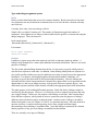
Table of Contents
I. Executive summary
3
II. Summary of project objectives
4
III. Description of ArbiTER functionality and usage
5
IV. Fluid tests and applications
8
V. Kinetic tests and applications
10
VI. Other tests and applications
12
VII. Conclusions
15
Acknowledgements
16
References
16
Appendix A: Summary of project publications and presentations
17
Appendix B: Summary of parallelization scaling studies
18
Appendix C: ArbiTER User’s Guide†
20
Appendix D: Eigenvalue solver for fluid and kinetic plasma models in
arbitrary magnetic topology†
21
Appendix E: Phase I report†
22
Appendix F: Full divertor geometry ArbiTER – 2DX benchmark
23
Appendix G: Listing of tutorial examples and simple verification tests
24
† paginated separately within
ArbiTER Final Report, page 2
Lodestar Research Corporation
Baver, Myra and Umansky
I. Executive summary
In this report, we discuss a new code for discretizing and solving eigenvalue problems in
diverse geometries. This code is called the Arbitrary Topology Equation Reader, or ArbiTER.
This code builds off the framework of the 2DX1 code, also developed by Lodestar Research
Corporation in collaboration with LLNL. In both cases, the codes are designed for exceptional
flexibility, which is achieved by loading model equations as input files rather than writing them
into the source code itself. The ArbiTER code adds to this flexibility by allowing topology, or
grid connectivity, to be loaded as an input file as well. This extra capability allows ArbiTER to
handle new or complicated geometries, allows the number of dimensions in the model equation
to be varied, and ultimately allows it to handle the types of equations used to model kinetic
physics.
Compared to time evolution codes, such as BOUT++2, eigenvalue solvers have the
advantage of superior computational efficiency when solving linear model equations, i.e.
problems can be solved faster and with fewer computational resources. Most eigensolver
packages, however, are difficult to use. Also, converting model equations into matrix form is
often nontrivial and prone to programming errors. By creating an integrated package to
discretize equations from an intuitive input format and then solve the resulting matrix equations,
the process of using an eigensolver is greatly simplified, allowing faster and more reliable setup
of new model equations.
This type of code is valuable for validation and verification (V&V). In addition, it can
also be used for primary physics studies. Its rapid reconfigurability makes it well-suited to
filling gaps in the computational capabilities of the community as a whole.
The team has successfully completed the majority of ArbITER project objectives.
Section II reviews the status of each objectives in detail. In summary, the required topology
language features were developed, implemented and tested in a number of benchmark cases.
Unstructured grid finite element analysis was added, kinetic capabilities of the code were
demonstrated for both parallel (Landau) and perpendicular (gyro-kinetic) problems, and a
source-driven mode of operation was developed. Integration of the ArbITER coding with the
parallel version of the SLEPc3 eigenvalue solver (an open source package not developed by the
project) was completed; however, we were not able to achieve good parallel SLEPc performance
in our application.4 Finally a number of structure and topology files have been created for
demonstration purposes and for standard cases of interest.
Section III of this document provides a brief description of ArbiTER functionality and
usage. A more complete and description is provided in a technical report prepared for publication
ArbiTER Final Report, page 3
Lodestar Research Corporation
Baver, Myra and Umansky
and included as Appendix D. Various fluid, kinetic and other ArbiTER test cases and
capabilities are summarized in Secs. IV – VI of this report, including 2DX emulation, Snowflake
geometry, extended domain calculations for separatrix spanning modes and Finite Larmor radius
stabilization of interchange modes. Among other items, the Appendices contain a summary of
project publications and presentations, some details of the parallelization scaling studies, and an
ArbITER User’s Guide.
II. Summary of project objectives
In the Phase I proposal, there were four objectives listed, all of which were completed:
(i)
(ii)
(iii)
(iv)
develop basic features of the new topology language
create topology language input files to replicate 2DX functionality for benchmarking
purposes.
perform benchmark cases that extend beyond 2DX functionality
perform code timing to motivate future parallelization
In the Phase II proposal, there were 14 objectives listed. Their description and status is as
follows:
(1)
(2)
(3)
(4)
(5)
(6)
(7)
Complete integration of SLEPc parallel solver with ArbiTER code. Complete. Test
results are shown in Sec. VI and Appendix B.
Perform profiling and optimization of ArbiTER code. Complete. Code has been
profiled, and optimization yields significant gains on a local workstation, but these
gains have not proven transferrable to a supercomputer.
Implement .hdf5 file input/output. Complete.
Introduce unstructured grid/finite element analysis capabilities. Complete. Test results
are shown in Sec. VI.
Add features to topology language in anticipation of proposed test problems. Complete.
Current topology language features are sufficient for all test problems.
Expand benchmarking of ArbiTER against 2DX. Complete. In addition to the test cases
from the Phase I project, the extended domain method was also benchmarked against
2DX.
Run verification problems, such as cyclotron/Landau damping, 5D wave damping, EM
cavity modes, and lattice vibrational modes. Complete. While the cases tested are very
different from the examples given, a number of new model equations were tried, and in
the case of the extended domain method the results were compared to 2DX.
ArbiTER Final Report, page 4
Lodestar Research Corporation
(8)
(9)
(10)
(11)
(12)
(13)
(14)
Baver, Myra and Umansky
Integrate with PETSc matrix solver to create source-driven code. Complete. Test
results are shown in Sec. VI.
Develop user-friendly routines to assist in structure and topology file creation.
Incomplete. Structure and topology file creation is essentially the same as at the end of
Phase I.
Develop routines to assist in grid file generation. Complete. New Mathematica
worksheets are able to construct grid files in a general way based on topology
information provided by a variant build of the ArbiTER code.
Develop user-friendly viewers for input, output, and data analysis. Complete. New
Mathematica worksheets are able to view data based on topology information from a
variant build of ArbiTER as well as infer topological features from the data itself. This
capability means that new worksheets do not need to be created every time a new
topology is used.
Benchmark ArbiTER against BOUT++. Incomplete. This was not considered a high
priority since ArbiTER is already extensively benchmarked against 2DX, and 2DX is
benchmarked against BOUT++.
Benchmark ArbiTER against COGENT. Incomplete. Divergent priorities between
ArbiTER and COGENT have not permitted such a comparison.
Develop structure/topology files used in all tests into standard libraries. Coding for
every application example in this report has been archived.
III. Description of ArbiTER functionality and usage
The ArbiTER code borrows significant features from the 2DX code. In particular, it uses
an equation language to define model equations, giving it a high degree of flexibility with
regards to physics models. Unlike the 2DX code, instead of being restricted to a single
predefined geometry, ArbiTER uses a topology language to define its computational grids.
Most of the features described in this section are also described in Appendix D, but are
repeated here for the sake of clarity.
A. Equation language
Much of the flexibility of the ArbiTER code derives from a feature it inherits from 2DX,
namely, the use of an equation parser to specify the physics model to be solved. The input file
for this equation parser is referred to as a structure file. Because the equation parsers used by the
ArbiTER Final Report, page 5
Lodestar Research Corporation
Baver, Myra and Umansky
two codes are relatively similar, it is a straightforward process to convert 2DX structure files into
ArbiTER format.
The structure file has three major parts. The first is the label list, which determines how
the grid file will be parsed. The grid file contains all information specific to a particular instance
of a physics model, such as scalar parameters, profile functions, and so forth. Its format consists
of a series of data blocks, each of which is assigned a label. The label list assigns each label a
variable type (integer, real scalar, real function, complex function, integer array), an index
number, and in the case of array data, a topological domain.
The second is the formula language, which governs construction of systems of equations
from simpler building blocks. For instance, if we take the second equation in the resistive
ballooning model,
∙
this might be coded as
gg*(1+0j)*N=(-1+0j)*kbrbpx*n0p*PHI
where gg is the structure file notation for the eigenvalue , complex constants are in parenthesis,
N =N, and PHI = are field variables, and kbrbpx and n0p represent a function and input
profile, respectively. Here j = (1)1/2 so, for example, 1+0j represents the complex number 1.
The third is the element language. The element language allows complicated functions or
operators to be derived from simpler building blocks. This is accomplished through a series of at
most binary operations. Thus, an operator of the form:
||
∂
might be represented through a series of instructions such as the following:
xx=xjac
load function into function buffer
xx=interp*xx
multiply function buffer by operator interp
tfn1=xx
place result in function tfn1
yy=ddyu
load operator ∂ into operator buffer
yy=tfn1*yy
multiply operator buffer by function tfn1
op1=yy
place result in operator op1 (
|| )
The ArbiTER equation parser, while it is reverse-compatible with the 2DX equation
parser, has a number of additional capabilities. It is capable of performing arithmetic operations
ArbiTER Final Report, page 6
Lodestar Research Corporation
Baver, Myra and Umansky
on constants (these are treated as “functions” on a domain with one node), an ability lacking in
2DX (which could only perform arithmetic operations on constants if the operation also involved
a function). In addition, many built-in functions in Fortran 90, such as trigonometric functions,
are now accessible through the ArbiTER equation parser as well.
B. Topology language
The main distinguishing feature of ArbiTER is its topology parser. The topology input
file consists of a series of topology element definitions. There are five different types of
topology elements. Bricks (Cartesian sub-domains) and linkages (lists of connected node pairs)
form the most basic topology elements. From these, domains (complete spaces) and operators
(sparse matrices) are constructed. The fifth element type, the renumber, is used to modify node
ordering in domains so as to permit intuitive ordering of elements in the grid file.
Of these, linkages and domains have an enormous variety of sub-types. It is from the
diversity of these elements that ArbiTER gains its tremendous flexibility and versatility. In their
simplest sub-types, linkages simply connect one edge of a brick to the opposing edge of another
brick (when used to create domains), or link each point in a domain to an offset point in the same
domain (when used to create operators); domains are simply sets of bricks pasted together by
their relevant linkages. However, other sub-types allow for more advanced operations. Domains
can be indented (have points removed from certain edges of an existing domain to facilitate
staggered grids), can be convolved (constructed from an outer product of two existing domains
to generate a higher-dimensional space), or can be masked (have points removed from an
existing domain according to a list). Linkages can include phase-shift information (useful, e.g.
for field-line following coordinates in closed field line toroidal topology), can remove phaseshift information incorporated into an existing domain, can locate boundary conditions, can link
convolved domains, can be explicitly defined based on grid coordinates, can be explicitly
defined from a list, or can have variable offsets.
This flexibility gives the code capabilities far exceeding that of the 2DX code, and
significantly exceeding its own probable or intended uses. ArbiTER can handle unstructured
grids and arbitrarily shaped domains. It can handle equations involving higher numbers of
dimensions, including equation sets in which different variables have different numbers of
dimensions. It can handle arbitrary-order differential operators, or integral operators of variable
footprint size.
ArbiTER Final Report, page 7
Lodestar Research Corporation
Baver, Myra and Umansky
C. Variant builds
In order to accommodate a wide variety of features and functions, a number of variants of
the ArbiTER code were constructed. These variants are implemented via different makefiles,
such that a common set of source code files are shared by all builds; only a small portion of the
source code, which is isolated into separate files, changes with each build. This prevents errors
due to updates in the main source code failing to be incorporated into variant codes.
Some features implemented via these variant builds include:
o Ability to solve source-driven problems.
o Ability to generate matrices for use by a stand-alone eigensolver.
o Ability to use HDF5 input/output. This was implemented as a separate build
because not all platforms that run ArbiTER have HDF5 libraries installed.
o Ability to run in parallel. This was implemented as a separate build because
parallel execution is much less convenient than serial execution, and because
there is no reason to discard code used in serial execution.
These variants are discussed in further detail in Appendix D section II.C.
IV. Fluid tests and applications
A. 2DX emulation tests
In order to verify the ability of ArbiTER to emulate the capabilities of the 2DX code, the
ArbiTER code was used to solve a resistive ballooning model. This was chosen because it is a
simple test that was already used to benchmark the 2DX code, hence data was readily available
for comparison. The structure file in this case contains a three-field model, describing the
evolution of potential, density, and the parallel component of vector potential. The topology file
describes an x-point topology, with operators defined so as to emulate 2DX. The results show
excellent agreement between the two codes, consistent with both codes producing the same
matrix within the limits of round-off error. This case is described in more detail in Appendix F.
B. Snowflake geometry
A particularly useful and timely application of the ArbiTER code is modeling plasma
instabilities in the complex magnetic topologies associated with the snowflake divertor.5,6 Such
instabilities are important for determining the scrape-off layer width, among other transport
properties. Because of the novelty and complexity of this divertor geometry, few other codes
have the ability to model it, creating a niche for ArbiTER’s topological flexibility.
ArbiTER Final Report, page 8
Lodestar Research Corporation
Baver, Myra and Umansky
The geometries used in this test were based on DIII-D data, and were provided in a
format suitable for the UEDGE code. A conversion script written for Mathematica was used to
convert this data into ArbiTER format. An innovative feature of this script was the use of a
variant build of the ArbiTER code (arbiterfd) to replicate the grid used in the original UEDGE
data, including topological features. This was used by Mathematica to separate the data into
topological regions, from each of which was constructed an interpolation function. These
interpolation functions were then used to map the data onto a second grid with a different
number of grid points. The advantage of this approach is that the Mathematica script does not
need to be written specifically for each topology, but instead will work for a broad class of
topologies. This avoids the issue of having to code topology twice, once for ArbiTER and once
for grid setup; instead, the same topology coding (the ArbiTER topology file) is used to perform
both functions. This case is described in more detail in Appendix D section III.A.
C. Extended domain for separatrix spanning modes
When applying a field-line following coordinate system to the closed field line region of
a tokamak, it is necessary to introduce a branch cut where a phase-shift periodic boundary
condition is applied.1 For low to moderate toroidal mode numbers, this solution works just fine.
However, at high toroidal mode numbers, the phase shift can exhibit such rapid radial variation
as to be underresolved, or to dominate the resolution requirements of that model. The extended
domain method represents an alternate approach in these cases.
In the extended domain method, the computational domain extends around the torus
multiple times. Each transit increases the cumulative magnetic shear of the coordinate system,
so that at the periphery of this extended domain the mode develops a high radial wavenumber
which in turn causes it to evanesce rapidly to zero. As a result, the mode is localized near the
center of the extended domain. If the extended domain makes enough transits around the torus,
the mode amplitude at the ultimate edge of this domain can be made negligible. Superimposing
the solutions from the various transits then provides the physical solution, as in the standard
ballooning formalism.7,8 This technique or related ones are routinely use by the community for
codes that work entirely on a closed surface domain. However, the ArbiTER implementation is
the first one, to our knowledge that permits simultaneous treatment of closes and open field line
regions, thereby allowing for the first time extended domain treatment of separatrix spanning
modes.
The ArbiTER code is particularly well suited for this approach because it is possible to
take a normal 2D x-point domain and project it in a third dimension to create multiple copies of
that domain. Using an offset linkage where the branch cut would otherwise be links these copies
ArbiTER Final Report, page 9
Lodestar Research Corporation
Baver, Myra and Umansky
together to form a domain of suitably multiplied length. This case is described in more detail in
Appendix D section III.E.
V. Kinetic tests and applications
A. Langmuir waves
One of the key advantages of the ArbiTER code is its ability to solve kinetic model
equations. In order to demonstrate this capability, it is necessary to use a physics model that
contains the essential characteristic of a kinetic model, namely that the model couples variables
in real space to variables in a higher-dimensional phase space. It is moreover desirable that this
capability be tested using as simple a model as possible.
This was addressed by using a modified Vlasov equation to model Langmuir waves.
This results in only a 2D model, hence it does not push ArbiTER’s capacity for high-dimensional
models beyond that of 2DX. However, because the potential equation operates in a 1D real
space, the ability to couple these spaces demonstrates a key capability in the solution of kinetic
model equations. The model equations and test results are covered in more detail in Appendix E
in sections III.B and IV.B.
B. Kinetic ballooning modes
While the Langmuir wave model may be useful in demonstrating the basic capabilities
necessary for a kinetic model, most kinetic models are far more complicated and involve larger
numbers of dimensions. Thus, a model with some element of real geometry is desired.
Moreover, it is helpful if the solution to this model can be compared to solutions of the same
physical problem under simpler or possibly semi-analytic models.
The model of choice for this purpose was a kinetic resistive ballooning model. In this
model, a resistive ballooning model was modified to include kinetic physics, such as Landau
damping. This results in a model that deviates from fluid theory in a distinctive way in certain
parameter regimes. The model equations and test results are covered in more detail in Appendix
D in section III.B.
C. Finite Larmor radius stabilization of interchange modes
While the above tests demonstrate the ability of ArbiTER to solve kinetic models,
gyrokinetic equations present unique challenges. To solve such equations in a numerically
efficient manner, new capabilities were added to the code.
ArbiTER Final Report, page 10
Lodestar Research Corporation
Baver, Myra and Umansky
The challenge presented by gyrokinetic models comes in the form of the gyro-averaging
operator. This integral operator accounts for the fact that such models describe the motion of
particles’ guiding centers, rather than the motion of the particles themselves. Thus, electric and
magnetic fields are modeled in real space, whereas particle motion is modeled in guiding center
space. To convert between the two spaces, an operator such as the following is used9-11:
This operator is usually represented in wavenumber space. Such a representation can be
implemented in a numerically efficient manner in a time-stepping code through the use of fast
Fourier transforms. In an eigensolver, by contrast, fast Fourier transforms reduce to ordinary
non-sparse matrices. The use of non-sparse matrices vastly increases the computational cost to
solve the resulting eigensystem matrices. Such a trade-off is of dubious value given that the
computational cost of a full gyrokinetic model is typically already quite high, since such models
can operate in up to five dimensions. To preserve sparsity, it is desirable to represent this
operator in real space.
Fortunately, such a representation is relatively straightforward, due to the fact that the
original operator is modeling the average charge distribution of a particle with a finite orbit
radius. Moreover, the resulting representation is compactly supported, i.e. the value of the
integrating function is zero outside some finite interval. To take advantage of the sparsity
created by this finite operator footprint, it is necessary to introduce a feature to permit integral
operators of variable footprint width.
This capability is provided by a type of linkage called a sheared linkage. A sheared
linkage is offset by a variable amount depending on position. This provides capability for
variable footprint operators when combined with convolved linkages, which map each point in a
convolved domain to or from its corresponding point in the original domain. In this case, one
begins by constructing a convolved domain from the phase space and a dummy domain of size
equal to the footprint operator. On this space, one defines the integrating function. A sheared
linkage links each point in the integrating function domain to a point that maps to the point in
phase space that that particular element of the integrating function controls the interaction with.
Multiplying through by elementary integral operators (from the convolved linkage) and their
transposes yields an integral operator on the phase space.
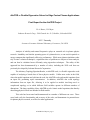
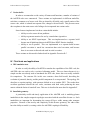
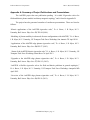
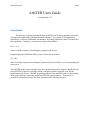
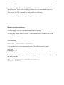
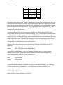
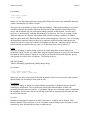
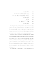
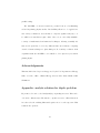
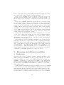
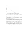
The test is performed on a kinetic interchange model, using the following equations:
ArbiTER Final Report, page 11
Lodestar Research Corporation
Baver, Myra and Umansky
where is the linear growth rate (the sought after eigenvalue), h is the unknown perturbed
distribution function, kb is the binormal wavenumber (to B and the radial direction), vD is the
grad-B drift velocity,  is the perturbed electrostatic potential, f0 is the equilibrium distribution
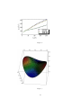
function, and is the plasma dielectric. The results of this test are shown in Fig. 1.
Fig. 1 Demonstration of gyro‐kinetic averaging in ArbiTER. Shown above are the results for the normlaized growth rate of a curvature driven interchange mode plotted against the product of the wave‐number kb and gyroradius parameter rL. When gyroaveraging is operative the mode stabilzes at large kbrL. VI. Other tests and applications
There are a number of capabilities of the ArbiTER code that are included not so much
because of anticipated applications within the plasma physics community, but rather because
they are easy to implement within the topology language framework and open up diverse
potential future applications. Most of these capabilities are related to the use of domains with
irregular boundary conditions. Problems of this type might include modeling of physics near the
divertor plate, where the shape of the divertor could be important, or modeling of RF antennas,
as the geometry of the antenna will have a significant effect on the plasma and surrounding
fields. To this end, two capabilities are of interest: masked domains, and unstructured grids.
ArbiTER Final Report, page 12
Lodestar Research Corporation
Baver, Myra and Umansky
In addition, the ArbiTER code has the ability to solve source-driven problems. The full
potential of this capability in plasma applications has not yet been explored, but it has been
demonstrated for simple test problems.
A. Masked domains
One way to model irregular boundary conditions is to first construct a domain with
regular boundaries, then selectively remove points from the grid until the correct shape is
achieved. This is accomplished using masked domains. A masked domain is a topology
language instruction that creates a domain from an existing domain, and a function defined on
that domain. Wherever the function is above a certain threshold, the point is not included in the
new domain. This allows the grid file to explicitly specify the shape of the domain. The concept
is loosely related to the volume penalization method12 where function values on the excluded
domain points are suppressed by volumetric terms added to the model equations. However, with
masked domains the grid points are actually removed from the computation.
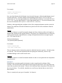
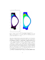
Demonstration of this feature was accomplished using a diffusion equation:
T
Taking the square root of the eigenvalue yields a wave equation:
T
Since the eigenfunctions are the same in either case, the only practical difference between
the two cases from a numerical point of view is in their boundary conditions: a diffusion
equation will typically use fixed-value (zero-value) boundary conditions, whereas a wave
equation will typically use zero-derivative boundary conditions.
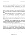
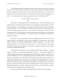
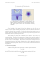
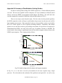
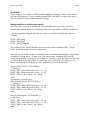
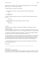
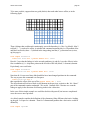
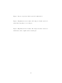
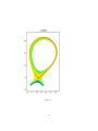
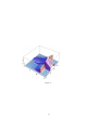
Examples of this are shown in Fig. 2. This figure shows a number of eigenmodes from a
diffusion/wave equation in a star-shaped resonator. The figure on the left shows a solution with
zero-value boundary conditions (consistent with a diffusion equation) whereas the figure on the
right shows a solution with zero-derivative boundary conditions (consistent with a wave
equation). Both are consistent with the expected physical solutions.
B. Unstructured grids
While most of the test problems so far have used finite difference methods, the ArbiTER
code is also capable of solving equations using finite element methods. Finite element methods
rely on the weak formulation, in which a partial differential equation is represented by a
superposition of basis functions:
ArbiTER Final Report, page 13
Lodestar Research Corporation
Baver, Myra and Umansky
Fig. 2 Demonstration of eigenmodes in masked domains. Left: diffusion equation solution with zero‐value boundary conditions; right: wave equation solution with zero‐derivative boundary conditions Given knowledge of the integrals of these basis functions over each cell, one can
construct a matrix equation describing the interaction of these basis functions and from this
calculate the function values at each node. For first-order elements, these integrals are easy to
perform, and the main complexity derives from the need to keep track of the properties of the
cells and their connectivity to their respective nodes.
These problems are solved with a combination of two features. One is the use of
convolved domains. This allows for the construction of a domain of size equal to the number of
cells time the number of nodes per cell, sufficient to store information about node connectivity.
The other is the use of listed linkages. This permits the construction of a linkage between the
aforementioned domain and the domain containing nodes, with the appropriate connectivity
information provided by the grid file. This test, as well as its results, are discussed in more detail
in Appendix D.
C. Source-driven capability
In addition to being able to solve eigensystems, or matrix equations of the form:
the ArbiTER code also has the ability to solve ordinary matrix equations, of the form:
ArbiTER Final Report, page 14
Lodestar Research Corporation
Baver, Myra and Umansky
These equations are called source-driven because the typical physics application consists
of calculating the response of a system to a known perturbation, such as a resonant magnetic
perturbation (RMP) or an RF field. Having this capability therefore greatly extends the potential
applications of this code, at relatively little cost in terms of code development.
This capability exists first because the primary function of the ArbiTER code is to generate
matrices; what is later done with them is not as important. Second, ArbiTER uses the SLEPc
package to solve eigensystems; this package runs on top of the PETSc13 linear algebra package,
which includes a satisfactory suite of matrix solving routines.
In order to demonstrate the source driven capabilities of the code, we chose the problem
of a magnetic dipole oriented transversely in a perfectly conducting cylinder. This problem was
chosen because it is nontrivial yet has a readily available analytic solution. This test, and its
results, are discussed in more detail in Appendix D.
D. Integrated parallel code and scaling studies
One of the key objectives of the ArbiTER project is the development of an integrated
parallel code. This is particularly important for kinetic and gyrokinetic applications, where the
number of nodes in the computational grid can become extremely large, thus becoming
impractical to solve on a single processor. By modifying the code to take advantage of modern
supercomputing resources, its potential applications are greatly increased.
Much of these parallel computing capabilities are already included in the SLEPc
eigensolver package. Therefore, the aim of this portion of the project was 1) to interface with the
parallel capabilities of the SLEPc solver in an efficient way, and 2) to test the capabilities of the
SLEPc package in a parallel environment. In these goals, objective 1 was successfully
completed. Objective 2, however, demonstrated that optimization of the SLEPc eigensolver in a
parallel environment is at best nontrivial. Associated test results are described in more detail in
Appendix B.
VII. Conclusions
As should be evident from the preceding summary, and the detailed appendices, the
ArbiTER project has been successful in developing a versatile and flexible computational tool
for application to edge physics problems in magnetic fusion plasmas, and has potential for many
other applications as well.
This code has been verified and demonstrated through a wide variety of test problems.
These range from problems of direct relevance to edge plasma physics, such as resistive
ArbiTER Final Report, page 15
Lodestar Research Corporation
Baver, Myra and Umansky
ballooning stability of snowflake divertors, to problems that showcase more exotic capabilities,
such as finite element analysis. In addition, mathematical techniques required for gyrokinetic
simulations were developed and tested, and studies were done on the parallel scaling of the code
and its underlying eigensolver package.
Acknowledgements
This material is based upon work supported by the U.S. Department of Energy Office of
Science, Office of Fusion Energy Sciences under Award Number DE-SC0006562.
References
1.
D. A. Baver, J. R. Myra and M.V. Umansky, Comp. Phys. Comm. 182, 1610, (2011).
2.
M.V. Umansky, X.Q. Xu, B. Dudson, L.L. LoDestro, J.R. Myra, Computer Phys. Comm.
180, 887 (2009).
3.
http://www.grycap.upv.es/slepc/
4.
More extensive experimentation with iterative linear solvers and upgrades to SLEPc since
the version tested (3.3) provide possible paths to improved parallel performance. Project
time constraints did not permit further progress in this area. Nevertheless, SLEPc
performance proved to be more than adequate for the applications discussed here, and
SLEPc is certainly an outstanding eigenvalue solver on a single processor.
5.
D. D. Ryutov, Phys. Plasmas 14, 064502 (2007).
6.
M. V. Umansky, R. H. Bulmer, R. H. Cohen, T. D. Rognlien, and D. D. Ryutov, Nucl.
Fusion 49, 075005 (2009).
7.
J. W. Connor, R. J. Hastie, and J. B. Taylor, Proc. R. Soc. London 365, 1 (1979).
8.
R. L. Dewar and A. H. Glasser, Phys. Fluids 26, 3038 (1983).
9.
E. A. Belli and J. Candy, Phys. Plasmas 17, 112314 (2010).
10. H. Sugama and W. Horton, Phys. Plasmas 5, 2560 (1998).
11. X. S. Lee, J. R. Myra, and P. J. Catto, Phys. Fluids 26, 223 (1983).
12. B. Kadoch, D. Kolomenskiy, P. Angot and K. Schneider, J. Comp. Phys. 231, 4365 (2012).
13. http://www.mcs.anl.gov/petsc/
ArbiTER Final Report, page 16
Lodestar Research Corporation
Baver, Myra and Umansky
Appendix A: Summary of Project Publications and Presentations
The ArbiTER project has one publication pending. It is titled “Eigenvalue solver for
fluid and kinetic plasma models in arbitrary magnetic topology” and is listed in Appendix D.
The project has also generated a number of conference presentations. These are listed as
follows:
“Kinetic applications of the ArbiTER eigenvalue code,” D. A. Baver, J. R. Myra, M. V.
Umansky, Bull. Amer. Phys. Soc. 59, TP8 48 (2014).
“Modeling of plasma stability in advanced divertor configurations with ArbiTER,” D. A. Baver,
J. R. Myra, M. V. Umansky, US Transport Task Force Workshop, San Antonio TX April 2014.
“Applications of the ArbiTER edge plasma eigenvalue code,” D. A. Baver, J. R. Myra, M. V.
Umansky, Bull. Amer. Phys. Soc. 58, PP8 37 (2013).
“Status of the ArbiTER kinetic eigenvalue code,” D. A. Baver, J. R. Myra, M. V. Umansky, US
Transport Task Force Workshop, Santa Rosa CA April 2013.
“Upgrades to the ArbiTER edge plasma eigenvalue code,” D. A. Baver, J. R. Myra, M. V.
Umansky, Bull. Amer. Phys. Soc. 57, JP8 115 (2012).
“ArbiTER: a flexible eigenvalue solver for fluid and kinetic problems in general topologies,”
D. A. Baver, J. R. Myra, M. V. Umansky, US Transport Task Force Workshop, Annapolis MD
April 2012.
“Overview of the ArbiTER edge plasma eigenvalue code,” D. A. Baver, J. R. Myra, M. V.
Umansky, Bull. Amer. Phys. Soc. 56, JP9 91 (2011).
ArbiTER Final Report, page 17
Lodestar Research Corporation
Baver, Myra and Umansky
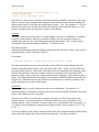
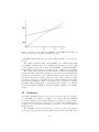
Appendix B: Summary of Parallelization Scaling Studies
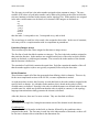
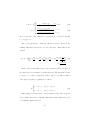
In order to test the parallel scaling of the SLEPc eigensolver, a 3D heat diffusion problem
was used. This was run in parallel on three computers: an 8-cpu workstation at Lodestar named
Abacus, and on two NERSC supercomputer named Hopper and Edison. The wall clock time
was then compared for a number of different sized grids and numbers of CPU’s.
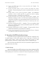
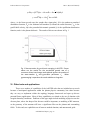
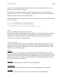
There are two major results from this study. The first is that, for this particular problem,
the SLEPc eigensolver scales well up to a small number of processors, but does not scale well for
larger numbers of processors. More generally, for the set of test problems we have used, and for
the set of SLEPc options we have explored (including hardware, compilation, and runtime
options) we were not able to achieve good scaling to more than a few processors. It remains to be
demonstrated that SLEPc can scale well to the type of problems relevant to ArbiTER. The
second result is that scaling is significantly better on the smaller computer (Abacus) than on the
NERSC supercomputers. This is summarized as follows:
1.00
0.70
tnorm
0.50
203
403
0.30
603
0.20
803
0.15
1.0
abacus
1.5
2.0
3.0
Ò processors
5.0
7.0
1.00
0.70
tnorm
0.50
0.30
203
0.20
0.15
403
603
0.10
1.0
1.5 2.0
nersc/hopper
3.0
5.0 7.0
Ò processors
10.0
15.0
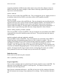
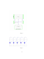
Fig. G‐1 Parallel scaling results for abacus and hopper computers In Fig. G-1, tnorm is the time to run the job normalized to the time required using a single
processor. The colors indicate the resolution of the problem in total grid cells. As can be seen,
ArbiTER Final Report, page 18
Lodestar Research Corporation
Baver, Myra and Umansky
scaling on Abacus is nearly ideal for this problem, but scaling on Hopper shows little
improvement beyond a few processors.
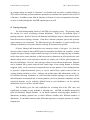
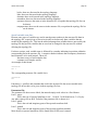
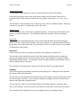
In order to gain insight into why scaling might display this behavior, the profiling options
in SLEPc were used to determine how much time was spent on each part of the calculation. This
operation was run on Abacus on 1, 2, 4, and 7 processors using problems of two different sizes.
The results of this are as follows:
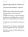
Fig. G‐2 Parallel scaling profiling tests. In this case, it appears that while some parts of the calculation scale relatively well, others
actually display reverse scaling, i.e. the total wall clock time increases as the number of
processors increases. Unfortunately, this did not shed sufficient insight into why these
operations were scaling so poorly or, more importantly, what to do about this. The result for
now is that, with the SLEPc options employed, using more than a few processors appears to be
counterproductive.
Thus, despite considerable effort, we were unable to achieve acceptable scaling with a
large number of processors on Hopper or Edison.4 However, having said that, it is also
important to note, as previously mentioned, that the eigensolver approach is very efficient
compared to time-stepping methods in terms of required CPU time. For example, tests discussed
in this report typically ran in a few minutes to at most an hour on a single processor.
ArbiTER Final Report, page 19
Lodestar Research Corporation
Baver, Myra and Umansky
Appendix C: ArbiTER User’s Guide
(This page intentionally blank. The User’s guide follows, with its own pagination.)
ArbiTER Final Report, page 20
Arbiter Users Guide page 1 ArbiTER Users Guide
Last updated 8-2-13
Introduction
The Arbitrary Topology Equation Reader (ArbiTER) is a flexible eigenvalue solver that
is designed for application to partial differential equations. It is capable of solving physical
problems by a variety of mathematical techniques. Its primary limitation is that it is restricted to
linear problems. Currently, it can only solve eigenvalue problems:
Blx=Ax
where A and B are matrices describing the equations to be solved.
Proposed upgrades include the ability to solve source-driven problem:
Ax=Bb
where A and B are matrices describing the equations to be solved and b is a vector containing the
source term.
The ArbiTER kernel does not actually solve the equations listed above; these are handled by the
powerful SLEPc eigensolver package, which is integrated with the ArbiTER code in both
parallel and serial versions. Instead, the primary purpose of the ArbiTER code is in discretizing
differential equations, converting continuous PDE's into sparse matrices. This process is
performed in a number of steps, which are described in the following sections.
Arbiter Users Guide page 2 GettingStarted
In order to use the ArbiTER code, it is necessary to install the source code. This requires the
following steps:
InstallArbiTERsourcefiles
In the current version of ArbiTER, there are 12 source files and 10 makefiles. Verify that these
are present in your work directory. These are:
arbiops.f90
arbiter.f90
arbiterog.f90
arbiterm.f90
arbiterdi.f90
commonvars.f90
iops.f90
iopsh.f90
slepcops.F90
slepcopsd.F90
slepcopsp.F90
sparsevars.f90
amakes.mak
amakesh.mak
amakep.mak
amakeph.mak
amakeog.mak
amakeogh.mak
amakem.mak
amakemh.mak
amakedi.mak
amakedih.mak
InstallPETScandSLEPc
In order to run, the ArbiTER code needs to include files from the PETSc linear algebra package
and the SLEPc eigensolver package. Since SLEPc also requires files from PETSc, these need to
be installed together.
The current version of ArbiTER is designed to work with versions 3.3 of both PETSc and
SLEPc. Source code also exists to operate with versions 3.0, but this is not mutually compatible
with the current version.
Arbiter Users Guide page 3 InstallHDF5
If your computer does not have an HDF5 module installed, install one. Details on this step are
still under development. If you are unable to install HDF5, non-HDF5 versions of the source
code are included with the standard ArbiTER package.
Modifymakefilestoincludesourcepaths
ArbiTER comes with a set of makefiles to assist in installing the source code. In order to
operate, these must be modified to include the paths used in the SLEPc and PETSc installations.
After selecting and opening the makefile you wish to use, find lines defining the following
variables:
PETSC_DIR=[path]
SLEPC_DIR=[path]
PETSC_ARCH=[subpath]
The variable PETSC_ARCH should be the same one used when installing SLEPc. See the
SLEPc installation manual for more details on this.
Note that each set of path variables is embedded within commands identifying the computer that
the makefile is being run on. To make your own version, these commands should also be
modified to match the computer you are working on. Generally, a good idea here is to copy each
set of lines, then modify one of them to create a new set of instructions. For instance, if you
have a version designed for Abacus (a Linux workstation) you may find the lines:
ifneq ($ (findstring aba, $ (CPUNAME)),)
# - for abacus
PETSC_DIR = /home/derek/solver/petsc - 3.3 - p6
SLEPC_DIR = /home/derek/solver/slepc - 3.3 - p3
PETSC_ARCH = arch - linux2 - cxx - debug
endif
Copying these yields the lines:
ifneq ($ (findstring aba, $ (CPUNAME)),)
# - for abacus
PETSC_DIR = /home/derek/solver/petsc - 3.3 - p6
SLEPC_DIR = /home/derek/solver/slepc - 3.3 - p3
PETSC_ARCH = arch - linux2 - cxx - debug
endif
ifneq ($ (findstring aba, $ (CPUNAME)),)
# - for abacus
PETSC_DIR = /home/derek/solver/petsc - 3.3 - p6
SLEPC_DIR = /home/derek/solver/slepc - 3.3 - p3
PETSC_ARCH = arch - linux2 - cxx - debug
endif
Arbiter Users Guide page 4 If you want to run on Hopper (a large Cray), one of these can be modified to include the correct
PETSc and SLEPc installations:
ifneq ($ (findstring hop, $ (CPUNAME)),)
# - for hopper.nersc.gov
PETSC_DIR = /global/homes/u/umansky/PUBLIC /. HOPPER/PETSC_MPI _CRAY
_COMPLEX3/petsc - 3.3 - p1
SLEPC_DIR = /global/homes/u/umansky/PUBLIC /. HOPPER/SLEPC_MPI _CRAY
_COMPLEX3/slepc - 3.3 - p0
PETSC_ARCH = arch - cray - xt7 - pkgs - opt
endif
ifneq ($ (findstring aba, $ (CPUNAME)),)
# - for abacus
PETSC_DIR = /home/derek/solver/petsc - 3.3 - p6
SLEPC_DIR = /home/derek/solver/slepc - 3.3 - p3
PETSC_ARCH = arch - linux2 - cxx - debug
endif
Selectaversiontomake
In the current version there are 10 available makefiles. These each construct a distinct variant of
the code. These can be grouped roughly as follows:
amakes, amakesh, amakep, amakeph
These are use to make the executable "arbiter" which is the main version of the ArbiTER code.
These each solve an eigensystem as described above.
amakeog, amakeogh
These are used to make the executable "arbiterog" which is the operator/grid version of the
ArbiTER code. It is primarily used for debugging topology and structure files, as it returns
detailed information about the internal data generated in the process of constructing the
eigensystem matrices. It does not actually generate matrices or solve them.
amakem, amakemh
These are used to make the executable "arbiterm" which is the matrix version of the ArbiTER
code. It can be used either for debugging structure, topology, and grid files, or it can be used in
conjunction with a stand-alone SLEPc solver. This version returns the eigensystem matrices, but
does not actually solve them.
amakedi, amakedih
These are used to make the executable "arbiterdi" which is the diagnostic version of the ArbiTER
code. It is primarily intended to evaluate the relative strength of terms in a model equation. This
version inputs a vector containing the solution to a previous eigensystem, then multiplies it by a
matrix containing the right hand side of some subset of the original model equations. By
Arbiter Users Guide page 5 comparing amplitudes of different parts of the output vector or how they change as terms are
added or removed, the relative strength of these terms in affecting a particular eigenvalue or
eigenvector can be determined.
amakes, amakesh
These are serial versions of the ArbiTER code. They are designed to run on a single processor or
on machines where the local SLEPc version does not have MPI capability installed.
amakep, amakeph
These are parallel versions of the ArbiTER code. They are designed to run on multi-processor
machines where the local version of SLEPc has MPI capability enabled. Note that these have a
different output file format than the serial version, specifically each processor generates a
separate output file ending in a four-digit index corresponding to the processor generating it. A
separate script is required to merge these files into a single output file, if this is desired.
amakes, amakep, amakeog, amakem, amakedi
These are non-HDF5 versions of ArbiTER. They are designed to run on machines where HDF5
is not installed or where the installation path is not known. These perform input and output in
ASCII format.
amakesh, amakeph, amakeogh, amakemh, amakedih
These are HDF5 versions of ArbiTER. They are designed to run on machines where HDF5 is
installed and where the installation path is known or can be loaded as a module. They are
capable of performing file I/O in ASCII format (in this regard their capability is identical to the
non-HDF5 versions) but will always search for a .h5 file and preferentially use it if it is
available. If any .h5 inputs are used, an .h5 output file will be generated. The exception to this
is that the non-standard debugging/diagnostic versions (arbiterog, arbiterm, arbiterdi) do not yet
produce .h5 output, but still accept .h5 grid, structure, and topology files if they are available.
Also, parameter file and vector file input is not yet converted to .h5 capability.
Maketheversion
Each version can be built using the command:
make -f [makefile] [executable]
Prepareinputfiles
There are three mandatory and one optional input file for the standard version of ArbiTER. The
diagnostic version additionally requires a vector input file. The formats of these files are
discussed in the following sections.
Input files have standardized filenames. ArbiTER will only look for files with these filenames,
and will return an error message if any mandatory file is missing. The files and their functions
are:
Arbiter Users Guide page 6 Gridfile
Acceptable filenames are gridfile.txt and gridfile.h5. These files contain data pertinent to the
specific problem to be solved, such as geometry, profile functions, scalar parameters, and so
forth.
Structurefile
Acceptable filenames are structafile.txt and structafile.h5. These files contain systems of
equations to be solved, as well as instructions regarding the numerical methods to be used to
calculate differential operators.
Topologyfile
Acceptable filenames are topofile.txt and topofile.h5. These files elementary topological
information needed to define the computational domain of the problem. These include how
many dimensions are in the problem, how subdomains are connected to each other, and how
differential operators are to be constructed on their most basic level, i.e. which grid points are to
be compared when attempting to calculate a derivative via finite differencing.
Parameterfile
Acceptable filenames are pssfile.txt and pssfile.h5. These files contain values used in the "poor
man's spectral transform" in which a spectral transform is applied to matrices prior to passing
them to SLEPc, as opposed to relying on SLEPc's built-in spectral transform capability. This
feature was added in response to reliability issues with the command-line options to perform
spectral transforms in SLEPc. These issues may be related to changes in syntax for these
options, resulting in the old syntax not being recognized by newer versions. Presence of a
parameter file is completely optional and in fact is not recommended if command-line spectral
transform is to be used.
Vectorfile
Acceptable filenames are vecfile.txt and vecfile.h5. These files contain solution vectors to be
used by the diagnostic (arbiterdi) version of the code. They are not used by the standard version
of the code.
Runthecode
The ArbiTER kernel does not require any additional inputs at run time, since all input files have
standardized filenames. However, SLEPc requires a number of command-line inputs. Some
common inputs:
-eps_nev [n]: this specifies the number of eigenvalues to return. This can also be specified in
the grid file, but grid file input of this parameter is not reliably recognized by SLEPc.
-eps_ncv [n]: this specifies the size of the Krylov subspace. This parameter is optional, but most
problems require a value for this parameter that is much larger than SLEPc defaults in order to
converge efficiently. It must not be larger than the problem size, and must be at least as large as
-eps_nev (SLEPc default is double nev or problem size, whichever is less), but usually a value on
the order of 100 is sufficient.
Arbiter Users Guide page 7 -eps_largest_real: this flag specifies that SLEPc should prioritize the eigenvalues with the
largest real parts. This is useful in stability problems where the most unstable mode is of
interest.
Thus a typical ArbiTER command line might look like the following:
./arbiter -eps_nev 5 -eps_ncv 64 -eps_largest_real
Machine‐specificinstructions:
To run on Hopper at Nersc, some addition instructions are needed.
To configure to compile SLEPc at NERSC, certain modules must be loaded. Either use the
command:
module load [module]
or the command
module swap [current module] [new module]
if an existing module of equivalent function exists. The following must be loaded:
acml/4.4.0
PrgEnv-pgi/4.1.40
hdf5/1.8.8
In order to run the parallel version of the code on Hopper, it will be necessary to use the aprun
and qsub commands:
qsub –I –V –q interactive –lmppwidth=[# processors]
cd [working directory]
aprun –n [# processors] ./arbiter [options]
Arbiter Users Guide page 8 Datainput
As discussed in the previous section, the ArbiTER main code has three mandatory input files.
Grid file (gridfile.txt, gridfile.h5): this provides physical information about the problem,
such as physical parameters, profile functions, and physical locations of
grid points. It also contains the numerical size of a specific case.
Structure file (structafile.txt, structafile.h5): this provides information about the
equations to be solved. This includes instructions for building differential
operators in the specific coordinate system of the problem.
Topology file (topofile.txt, topofile.h5): this provides information about the numerical
domain on which the equations are to be solved. This includes connectivity and
number of dimensions. It does not include the size of the problem (this is
specified in the gridfile), but it does include instructions to calculate the size of
subregions of each domain based on values provided by the grid file.
This division reflects the ways that the data provided can be re-used to solve different problems.
Thus, many different physical parameters (grid files) can be simulated using the same equations
(structure files) and many different sets of equations (structure files) can be simulated using the
same numerical domains (topology files). Each of these is discussed in greater detail in the
section on input formats.
Input formats
Each of the three input files has a specific data format. In both ASCII and HDF5 versions, this
consists of a series of data blocks which are assigned a specific label. In the ASCII version, each
block may contain additional numbers specifying the size of each block. In the HDF5 version,
the size of each block is read as part of the HDF data describing the file.
In the case of the structure and topology files, these are additionally available in user-readable
and machine-readable forms. Conversion between the two is done using a series of Python
scripts. The machine-readable form is used by the ArbiTER kernel, while the user-readable form
is used to edit the files. The user-readable form contains significantly more data than the
machine-readable form (for instance, variable names) so should be retained in case any future
modifications to these files are needed.
Gridfile
The grid file accepts four types of data blocks. In addition, it also recognizes an end-of-file
indicator. Any data present after the end-of-file indicator is ignored. The number and types of
data blocks, as well as the block labels assigned to them, are controlled by the input language
section of the structure file.
The four data type are as follows:
Arbiter Users Guide page 9 integer: each block contains a single integer value.
real: each block contains a single real number.
real array: each block contains a list of real numbers. In ASCII format, this list is preceded by
an integer containing the size of the list.
integer array: each block contains a list of integers. In ASCII format, this list is preceded by an
integer containing the size of the list.
Structurefile
The structure file contains five sections, one of which is divided into four blocks for a total of
eight data blocks. There is also an end-of-file indicator which can be followed by comments. In
the user-editable form, there are the five sections found in the machine-readable structure file
plus an additional eight sections containing variable names. The sections are:
labels
Input language ("labelslist" in MR, "labels" in UR):
This section defines the data format of the grid file. Each entry in this section consists of a
descriptive label, followed by instructions on how to interpret the data.
In the machine-readable form, each label is followed by three integers. The first is the type of
data (integer, real, real array, integer array), the second is a unique index assigned to that data
block, and the third is the index of the domain on which an array is defined (only used for real
arrays).
In the user-readable form, each label is followed by a variable name and a domain name. In the
case of data blocks that do not require a domain name, the generic domain label "null" is used.
The type of data is inferred based on which list the variable name is declared in. Normally the
label and the variable name will be identical.
elements
Element language ("elementlang" in MR, "elements" in UR):
This section is used to create building blocks, or elements, that are used when constructing the
equation set. This allows the equations to be written in more compact notation, as well as
providing rules for constructing differential operators. Also, certain operator or function
definitions can be recycled from one equation set to another by simply copying this section (or
an appropriate subset) from one structure file to another.
The element language consists of a series of simple algebraic instructions that are executed
sequentially. Because of the restrictions placed on these instructions, a function buffer and two
Arbiter Users Guide page 10 operator buffers are included. These are assigned the standard labels of "xx" for the function
buffer and "yy" or "zz" for the operator buffers.
The following types of expressions are permitted:
1. Assign a buffer to a variable, a variable to a buffer, or a buffer to another buffer.
xx=dx
op2=yy
yy=zz
1a. Swap two buffers
yy<>zz
2. Apply an elementary arithmetic operation to a variable and a buffer, storing the result in a
buffer.
xx=xx+tip
xx=(2+0j)*xx
yy=tfn4*yy
3. Apply an operation with a name (rather than a symbol) to a buffer.
xx=exp xx
xx=abs xx
transpose yy
equations
Formula language ("mataheader","mataelements","matbheader","matbelements" in MR,
"equations" in UR):
This section defines the equations to be solved. In the user-readable form, this section consists
of a series of algebraic expressions. However, each expression must be in a very specific format:
1. Each side of each equation consists of a sum of terms. If terms are to be subtracted (rather
than added) this must be accomplished by multiplying those terms by -1.
2. On the right-hand side, each term must begin with a exactly one constant (i.e. a scalar number
which can be either a hard or soft constant) and end with a field (component of the solution).
The remaining parts of the term may be either functions or operators, but temporary functions
and temporary operators may not be used (these are only used by the element language).
3. On the left-hand side, the format is the same except that each constant is preceded by the
generic eigenvalue label "gg".
For instance:
gg*(-1+0j)*op4*fld6=(1+0j)*fun35*op4*fld6+(-1+0j)*fun36*op1*fld1
hardconstants
Hard constant list ("hardconstants")
This contains a list of hard constants used in the equation set. Each entry is loaded as a complex
number (as opposed to soft constants, which are loaded as real numbers but stored as complex
Arbiter Users Guide page 11 numbers). This is important as the definitions of basic complex numbers such as  and - are
typically stored in the hard constant list.
The division of constants into "hard" and "soft" is important because it keeps fundamental
parameters such as "2" or "-Â" out of the grid file, making the structure file more self-contained
and protecting these values from accidental change.
Each hard constant in this list is preceded by a label, usually a shortened version of the constant
itself. For instance:
(1+0j) (1.00000000000000,0.000000000000000)
-1j (0.00000000000000,-1.000000000000000)
(2+0j) (2.00000000000000,0.000000000000000)
(3.14159274101+0j) (3.14159274101257,0.000000000000000)
fields
Field list ("fielddomains" in MR, "fields" in UR):
This consists of a list of fields (quantities in the solution vector) that are used in the equation set.
Each field is assigned a domain. In the user-readable form, this section doubles as a list of
variable names, as the first string in each entry of this list is used as a keyword when the
conversion script parses the formula language.
Variablenamelists:
The user-readable form of the structure file requires variables to be assigned names, so as to
construct keywords for parsing other sections of the file and for identifying the type of object
referenced by each keyword. Eight such sections are used (in addition to the field list, which
doubles as a list of variable names):
integers
data consisting of a single integer, used by the topology file but defined in the structure file
because such data must be defined in the input language in order to be loaded from the grid file.
Note that this section must be identical to the corresponding section of the topology file, except
that it does not need to be as long (i.e. the topology file can contain additional entries in this
section, but no entries can be skipped).
functions
real/complex array data that is accessible to the formula language.
tempfunction
real/complex array data that is not accessible to the formula language (to save memory).
operators
differential operators (sparse matrices) that are accessible to the formula language.
Arbiter Users Guide page 12 tempoperators
differential operators that are not accessible to the formula language.
constants
real/complex scalar data.
domains
computational domains (defined by the topology file) that fields or real/complex arrays are
assigned to. Note that this section must be identical to the corresponding section of the topology
file, except that it does not need to be as long (i.e. the topology file can contain additional entries
in this section, but no entries can be skipped).
intarrays
integer array data.
Topologyfile:
The topology file contains four sections. In the user-readable form, this is supplemented by nine
lists of variable names. The sections are:
Integerlanguage("integerlang"):
This consists of a list of simple algebraic expressions that are executed sequentially. Its format is
similar to the element language of the structure file, but with the following differences:
-All data must be in scalar integer format. No real variables or functions are allowed.
-The buffer keyword "nn" is used instead of the keywords "xx", "yy", or "zz" used in the
element language.
-Absolute value is represented by placing the number in straight brackets, instead of
using the keyword "abs".
-Step and ramp functions s() and r() are defined, which describe a Heaviside function and
a Heaviside function times its argument, respectively.
-A buffer can be assigned an integer value directly, rather than first defining it as a
constant.
Examples:
nn=1
one=nn
nn=0
nn=nn-nxmis
nn=r(nn)
nn=|nn|
nxmim=nn
Topologylanguage("topoheader","topoelements"inMR,"topolang"inUR):
This section consists of a series of commands defining each topological object. There are five
basic types of objects, each of which may have one or more subtypes. These are:
Arbiter Users Guide page 13 Bricks: these are simple blocks of data points.
Domains: these are complex blocks of data points, that functions, operators, or fields can
be assigned to. They are constructed from bricks, and in the simplest case a domain may
just be a brick with a different assigned name.
Linkages: these are sets of rules that define a connection between two bricks or domains.
They can be used to tie together bricks into domains or domains into larger domains, or
they can be used to construct operators.
Operators: these are sparse matrices that define simple differential, integral, or other
operations. They are passed to the element language of the structure file as basic building
blocks for constructing more complicated operators.
Renumbers: these are instructions that change the sequencing of data points within a
domain. This sequence is important because functions are loaded from the grid file as
one-dimensional vectors without regard for any aspect of the domain it is to be assigned
to except its size. Thus, each domain should be sequenced according to the order in
which data points are likely to be read from the file.
The objects in the topology language are discussed in more detail in the following sections.
Defaulteigenvaluecounter("defaultnevs"):
This gives the name of the integer variable to be used when loading the number of eigenvalues to
be solved (nevs) from the grid file.
Defaultscalingcounter("defaultwci"):
This gives the name of the real/complex variable to be used to rescale eigenvalues prior to saving
them to the output file.
Historical note: ArbiTER is descended from the 2DX eigenvalue code. Since 2DX was
primarily designed to solve a 6-field Braginskii model with coefficients expressed in Bohm units,
a scaling factor was required to convert Bohm units back into real units (i.e. s-1). The appropriate
conversion factor is wci, so it became customary in development of the ArbiTER code to refer to
any eigenvalue scaling factor as wci. It may at first seem strange to have nevs and wci in the
topology file since they have nothing to do with topology per se. In addition to topology, the
topology file has the job of defining everything that was hard-coded in 2DX. This is so that the
ArbiTER kernel itself remains very general, but reverse compatibility of 2DX structure and
gridfiles is retained (as much as possible).
Variablenamelists:
As with the structure file, the user-readable form of the topology file requires variables to be
assigned names. Eight regular sections are used:
integers: data consisting of a single integer.
intarrays: integer array data.
Arbiter Users Guide page 14 bricks: these are discussed in the topology language.
links: these are discussed in the topology language.
domains: these are discussed in the topology language.
renumbers: these are discussed in the topology language.
operators: these are the same as in the structure file, except that the topology file list can
be shorter.
tempoperators: these are the same as in the structure file, except that the topology file list
can be shorter.
Specialvariablenamelists:
Because some types of variables are used in much greater numbers in the structure file than in
the topology file, a special type of list exists in order to declare only those variables that are
needed by the topology file. This has the added advantage that variables that are not used by the
topology file but precede variables that are used can be changed in the structure file without
affecting the topology file.
For these sections, each variable name is followed by a number indicating its position within the
corresponding list in the structure file. A negative number indicates that a temporary function or
hard constant is to be used instead. These are:
functions: arrays of real/complex data
constants: real/complex scalars
An example of this format:
constants
wci 1
The corresponding structure file variable list is:
constants
wci
Functions (i.e. profiles) and constants that used in the structure file but are not needed in the
topology file do not have to be given in these topology file lists.
Parameterfile:
The parameter file does not use labels, but instead simply reads values in a fixed format.
Line 1: sttype
This is the type of spectral transform to use. 1 is shift, 2 is shift and invert, 3 is Cayley.
Any other value gives no shift. Default (if the parameter file is absent) is 0.
Line 2: stshift
This is the real and imaginary parts of the spectral transform shift.
Line 3: astshift
This is the real and imaginary parts of the spectral transform antishift.
More details on spectral transforms can be found in the SLEPc user's manual.
Arbiter Users Guide page 15 Fileconversion
In order to convert input files between different file formats, a number of conversion tools are
included with the ArbiTER package to do this.
User to Machine format conversion
In order to convert structure and topology files between their user-readable and machinereadable forms, a set of Python scripts are provided:
edit2structa: converts user-readable structure files to machine-readable structure files.
structa2edit: converts machine-readable structure files to user-readable structure files.
(not yet available)
tedit2topo: converts user-readable topology files to machine-readable topology files.
topo2tedit: converts machine-readable topology files to user-readable topology files.
(not yet available)
ASCII to HDF5 format conversion
In order to to convert ASCII grid files, structure files, or topology files to HDF5 format, a pair of
programs are provided:
hconvgs.f90: converts grid and structure files to .h5 files. These conversions must be
done simultaneously, since the structure file is needed to read the ASCII grid file.
hconvt.f90: converts topology files to .h5 format.
Note in both cases that these programs convert machine-readable structure and topology files to
.h5 format, not the user-readable forms.
Arbiter Users Guide page 16 2DXemulation
Topology files exist that permit the ArbiTER code to emulate the capabilities of the 2DX code.
In order to use this capability, the 2DX structure file must be converted to ArbiTER format.
For the most part, the 2DX and ArbiTER structure files are nearly identical (at least in their userreadable form). However, there are some differences relating to how each code handles indented
variables (i.e. staggered grids).
To convert 2DX structure files to ArbiTER structure files, simply use the following step-by-step
instructions. Note that these apply to the user-readable form of the 2DX structure file, so it is
important to have those files available.
1. Drop the "x" from "xlabels". ArbiTER uses "labels" for this section instead.
2. Add a section called "domains" containing three domains. For a standard 2DX emulation
topology file, these are for standard, indented, and periodic boundary domains, respectively:
domains
ind0
indy
pbc
If these domain names are used, no further changes are needed in the "fields" section. If
different domain names are used, then the indentation indicators (ind0, indy) will need to be
replaced by their corresponding domain names.
3. Replace the w's and o's at the end of each label in the labels section with appropriate domain
labels. These are ind0 for standard variables and indy for indented variables. The only variable
to use pbc is q. If no domain label is appropriate, as for scalars, use "null."
Note that kpsii uses ind0, not indy, even though it is used exclusively as an indented variable,
because this conversion occurs later. Failure to note this will result in loss of ability to use
existing 2DX grid files.
2DX
ArbiTER
nevs nevs o
q q o
kb kb o
nevs nevs null
q q pbc
kb kb ind0
4. In the "constants" section, add two new constants: "onodx" and "onody". They are used by
the topology language to calculate differential operators.
2DX
ArbiTER
constants
dx
dy
constants
onodx
onody
dx
dy
Arbiter Users Guide page 17 5. Provide values for these constants by prepending the following lines of element language to
the beginning of the elements list:
xx=dx
xx=(1+0j)/xx
onodx=xx
xx=dy
xx=(1+0j)/xx
onody=xx
6. Rename (using find and replace) all temporary operators with numbers greater than 10. This
will help avoid label name collisions during the next step.
2DX
ArbiTER
tp11
tp12
tp13
tep11
tep12
tep13
7. Give descriptive labels (using find and replace) to the first 8 temporary operators, and delete
temporary operators 9 and 10 (these are not used in any existing structure file). This will help in
the next step.
2DX
ArbiTER
tp1
tp2
tp3
tp4
tp5
tp6
tp7
tp8
tp9
tp10
ddxu
ddxl
ddyu
ddyl
bc1
bc2
bc3
bc4
8. Insert the following operators to the temporary operator list: indented versions of the first two
differential and first two boundary operators, an interpolation operator, and a transfer operator.
ArbiTER
ddxu
ddxl
ddxui
ddxli
ddyu
ddyl
bc1
bc2
bc1i
bc2i
bc3
bc4
interp
itrans
Arbiter Users Guide page 18 9. Now comes the tricky parts. Go through the element language and find all instances of
elementary operators that have both indented and non-indented versions.
ddxu
ddxl
ddxui
ddxli
bc1
bc2
bc1i
bc2i
Figure out which domain the operator is supposed to be in based on context. Now, if an indented
operator is required (i.e. the operator will be operating on an indented variable) then replace it
with its indented version, i.e. ddxu->ddxui.
10. Replace all "interpolate" commands with multiplication by the operator "interp".
2DX
ArbiTER
interpolate xx indy ind0
xx=interp*xx
11. Make sure than any functions that are supposed to be loaded into the indented grid are at
some point multiplied by the operator "itrans".
2DX
ArbiTER
xx=kpsii
tfn9=xx
xx=kpsii
xx=itrans*xx
tfn9=xx
12. If you are using a structure file from one of the older versions of 2DX, you should strip out
any "transpose" commands. ArbiTER does not need transpose before matrix multiplication.
Note that recent versions of 2DX also do not need transpose before multiplication, so in that case
you may skip this step. Note that structure files that do not need this step will already be devoid
of "transpose" commands, so it never hurts to search for them just in case.
That should about do it. Note that the current version of the 2DX emulation topology file does
not support central differencing in y (ddyu+ddyl) because these operate on different domains.
This is an issue with some newer versions of the 6-field model. To upgrade these files, an
improved version of the topology file is needed. However, conversion to the new version will
not be significantly different, except that an extra temporary operator is used.
One could construct it as follows:
link simple ind0dyu
links ind0 ind0 dir 5 postofs domin dir 3 one
link simple ind0dyl
links ind0 ind0 dir 5 postofs domin dir 4 one
operator simple ddycd
+ind0dyu +ind0dyl *(.5+0j) *onody
Arbiter Users Guide page 19 Note that the following statements are equivalent (in the above context):
links ind0 ind0 dir 5 postofs domin dir 3 one
links ind0 ind0 dir 5 postofs domin dir 4 minone
Also note that ArbiTER uses a different edit-to-structure conversion script. The new script is
provided under the name "edit2structa". The extra "a" is not intended to make fun of Italians, but
rather to alter file names so as to permit side-by-side comparisons with 2DX.
Arbiter Users Guide page 20 Topologylanguageguide
Most sections of the topology file are fairly straightforward as described in the previous section.
The integer language functions essentially just like the element language in the structure file, and
the other sections are simply labels that designate particular variables as having special
significance. The topology language itself, on the other hand, is loaded with features and syntax.
This section will attempt to explain these features.
Basicstructure
Each entry in the topology language section of the topology file (user-readable form) consists of
two lines. The first line declares the type, subtype, and name of the topology element to be
created. The second line contains its argument list. For instance:
brick simple Edge
dimensions edgex edgey
The indentation of the second line is purely optional (the Python conversion script treats this as
whitespace) but is helpful for keeping track of which lines are element declarations and which
lines are argument lists. For every type of element, the syntax of the first line is exactly the
same: type, subtype, and name. The syntax of the second line, however, varies with the type and
subtype of element being declared.
Element declarations are evaluated sequentially. This means that if a topology element uses
other topology elements, those elements must be declared before the element that uses them.
Topology language execution begins before element language execution. However, topology
language execution will automatically go on hold if essential data is unavailable. Thus, if a
topology element requires a function that is not directly available from the grid file, topology
language execution will pause and element language execution will begin. This will continue
until the data required by the topology language has been generated. Once this occurs, topology
language execution will resume until all topology language instructions have been executed or
another piece of missing data is required.
Note that domains must be declared before the functions that occupy them. Thus, if topology
and element language instructions are poorly ordered, i.e. a topology language instruction
requires a function that is created later than a function that occupies a domain constructed later
than the aforementioned topology language instruction, an error will occur.
Arbiter Users Guide page 21 Typeandsubtypeargumentsyntax
Bricks
Bricks are basic data blocks that are used to construct domains. Bricks cannot be used on their
own (functions can only be declared on domains) but it is trivial to declare a domain with only
one brick in it.
Currently, there only exists one subtype of brick:
Simple: this is a simple Cartesian grid. The number of dimensions equals the number of
arguments. Each argument is an integer (either loaded from the grid file or constructed using the
integer language). Thus, the format is:
brick simple [name]
dimensions [dimension1] {dimension2} {dimension3}...
For instance:
brick simple nodesbase
dimensions nnodes
Linkages
Linkages are sparse arrays that relate points in one brick or domain to points in another. A
linkage can be thought of as a matrix plus additional associated information. There are two main
purposes of linkage.
The first is that, when building domains from bricks, it is necessary to specify which points in
each brick are adjacent to each other. In addition, when defining which points are adjacent it is
also useful to define whether any special conditions exist when crossing between the appropriate
boundaries. For instance, when applying phase-shift periodic boundary conditions, it is
necessary to specify the phase shift at each point along the boundary. Once the linkage and
affected bricks have been incorporated into a domain, these phase shifts are incorporated into the
domain data set, and it is no longer necessary to keep track of them as separate objects. Any
differential operators defined on this domain will inherit the appropriate phase shift information.
The other purpose is for building differential operators. Much like bricks, linkages cannot be
used directly for this purpose. However, it is relatively trivial to construct an operator that only
uses a single linkage. In this case, the purpose of the linkage is to define, when constructing a
finite difference operator, which points are next to a particular point for purposes of taking a
difference between function values at adjacent points. In other words, a linkage is needed to
define which point is one cell "higher" or "lower" in a particular direction. Since the domain in
question can have a complex internal topology, this is more complicated than simply
incrementing or decrementing a coordinate index. Note that linkages constructed on a domain
inherit properties of any previous linkages assembled into that domain.
There are currently seven types of linkages:
Arbiter Users Guide page 22 Simple
This type of linkage creates a linear correspondence between opposing edges or faces of two
bricks or domains. That is to say, it determines which points are on the appropriate edge of one
domain, and then determines which points in the other domain are adjacent to each point in the
first domain. The format for this is:
link simple [name]
links [left brick/domain] [right brick/domain] [direction] {offset 1 type}{offset 1
domain}{offset 1 direction}{offset 1}...
where [direction] consists of the keyword dir followed by an integer, e.g. dir 1
{offset 1 type} is either preofs or postofs
{offset 1 domain} is either domin or domout
{offset 1 direction} has the same form as [direction]
{offset 1} is the number of gridpoints to offset by
For instance:
link simple rotrbase
links cellc cellc dir 5 postofs domout dir 3 minone
where keywords have been bold color coded.
In this case, the link connects domain cellc to itself across direction 5, with a post-offset applied
on the right domain in direction 3 of amount minone (an integer variable, in this case having the
value -1). Several of these arguments require further explanation.
First, the directions. Each domain permits a number of directions to be defined equal to twice its
number of dimensions; the extra direction allows the opposite faces/edges of each linked domain
to be used. Thus, direction 1 links the right edge of the left domain to the left edge of the right
domain in dimension 1, whereas direction 2 links the left edge of the left domain to the right
edge of the right domain in dimension 1. Direction 3 does the same as direction 1 and 4 the
same as 2, but in dimension 2, likewise directions 5 and 6 affect dimension 3, etc.
dir
Edge of L-domain Edge of R-domain dim
1
R
L
1
2
L
R
1
3
R
L
2
4
L
R
2
…
…
…
…
2*nd+1
All points
All points
Another, and perhaps better way of thinking of dir is that dir 1 is the direction of increasing
index in the first (e.g. x) coordinate, dir 3 is increasing index in the y coordinate etc. Similarly,
dir 2 and 4 are in the direction of decreasing index. This definition of dir is more useful when
working with linkages.
Arbiter Users Guide page 23 dir
Index direction dim
1
increasing
1
2
decreasing
1
3
increasing
2
4
decreasing
2
…
…
…
2*nd+1
All points
Directions greater than twice the number of dimensions (i.e. that affect a dimension that does not
exist) treat the entire domain as an edge. In the above example, direction 5 happens to be greater
than twice the number of dimensions (cellc has only 2 dimensions) so the resulting linkage treats
the entire domain cellc as its own face, i.e. every single point is on the appropriate "edge" and
therefore eligible for inclusion in the linkage. This is useful for creating linkages that are
intended to be made into operators.
Second, the offsets. There are two basic types of offsets: pre-offsets, and post-offsets. Preoffsets change which point is used to initiate the linkage. Thus, a simple linkage normally begins
by finding one pair of adjacent points (one from each domain), then extending out along the
appropriate faces, matching neighboring points in one domain to their corresponding neighboring
points in the other domain. Normally, the starting pair is taken from matching corners of each
domain. If the starting pair is chosen differently, this displacement will be inherited by each
subsequent pair of points that are paired with each other.
The keywords domin and domout are used to indicate which side of the linkage the offset is
applied to.
domin
apply offset to the first (left) domain
domout
apply offset to the second (right) domain
A post-offset works differently: instead of changing the starting point, it creates a linkage
normally with no offset, then uses the internal connectivity of one domain to displace the
corresponding point in each pair. To put it another way:
preofs
postofs
offset then link
link then offset
Note that the offset part of the link command is optional.
Perhaps the simplest example of a linkage is for periodic boundary conditions. The following
example assumes Edge is a domain in (x, y) and edge2edge invokes periodic BCs in y.
link simple edge2edge
links Edge Edge dir 3
In this case dir 4 would work just as well as dir 3.
Arbiter Users Guide page 24 To be more explicit, suppose that two grids (bricks) abut each other but are offset, as in the
following figure
1
2
3
4
5
6
7
8
9
10
11
12
13
14
1
2
3
4
5
6
7
8
9
10
11
Then a linkage that would match continuously across the boundary (i.e. blue 1 to black 4, blue 2
to black 5, …). needs to be offset. A suitable link command assuming this is a 2D problem, blue
and black are bricks, three = 3 (defined in the integerlang) and the (x, y) directions are (across,
up) the page is
link simple blue2black
links blue black dir 3 preofs domout dir 1 three
Here dir 3 says that the linkage is in the second coordinate (y) and dir 1 says the offset is in the
first coordinate (x), i.e. skip three points on the left side of the left (black, i.e. domout) domain.
Equivalently, one could write
link simple black2blue
links black blue dir 4 preofs domin dir 1 three
Note that dir 4 is now used since black and blue have interchanged positions in the command.
The way to parse this command is to first parse
links black blue dir 4
then consider the effect of the rest of line preofs domin dir 1 three
The offset domin still refers to black (as did domout in the previous version) so the “dir 1 three”
part of the command remains unchanged. We use dir 1 instead of dir 2 because we want the
linkage to apply in the direction of increasing index in the x direction.
In the case of this simple example we could also do this with postofs, but in more complicated
cases the two are not equivalent.
As a third example consider the definition of the elementary finite difference derivative looking
up the grid. Let space be a domain. Then for 3-dimensional problem the x-derivative would be
defined by
link simple spacedxu
Arbiter Users Guide page 25 links space space dir 7 postofs domin dir 1 one
operator simple ddxu
+space *(-1+0j) +spacedxu *onodx
See below for a discussion of operators, but in this example it should be clear that we are using
links to create the upper diagonal matrix spacedxu, then (in the operator command) adding the
identity matrix space to spacedxu and multiplying by onodx = 1/dx. The constants (-1+0j), one,
onodx need to have been declared elsewhere in the topology filed and defined there (e.g. if an
integer) or defined in the structure file as a hard or soft constant.
Function
This type of linkage works the same as a simple linkage, except for one difference. In addition
to specify which points are linked by a particular linkage, one also specifies a function to
multiply function values by when displacing them along that linkage. This is mainly used to
create phase-shift periodic boundary conditions. The format here is:
link function [name]
links [left brick/domain] [right brick/domain] [direction] [link function] {offset 1 type}{offset 1
domain/function}{offset 1 direction}{offset 1}...
For instance:
links Edge Edge dir 4 linkfn pbcf2 preofs linkfn dir 1 nxmip
This particular instance exercises an option that is not available for simple linkages: the link
function, rather than either domain, can be the target of the offset. In this case, the offset does
not affect which points are connected to each other, but it does mean that when assigning values
from the link function to each pair of points, instead of counting from the beginning of the
function, it skips values (in this case, nxmip of them) before assigning a value to the first pair of
points. This displacement inherits properties of the domain to which the link function had been
assigned. So if the link function were defined in two dimensions, it would be possible to skip
points starting from any edge of that domain.
Convolved
This type of linkage is used in conjunction with convolved domains. The purpose of a
convolved linkage is to determine which points in the convolved domain correspond with which
points in the domains used to create them.
To make sense of this, let us first take a sneak peek at what we will later encounter in the
domains section. A convolved domain is a domain constructed as an outer product of two
existing domains. Thus, if domain 1 has three points (a, b, c) and domain 2 has four points (1, 2,
3, 4), then a convolved domain constructed out of these will have twelve points (a1, a2, a3, a4,
b1, b2, ...).
A convolved linkage, then, simply connects points in one of the original domains with the points
in the convolved domain that were generated from that point. The format for this is:
Arbiter Users Guide page 26 link convolved [name]
uses [domain 1] [domain 2] [domain 3] order [order]
For instance:
link convolved cell2cellc
uses cellc cell dimcon order 1
The significance of the domains depends on what order is used. In all cases, domain 1 is the left
domain and domain 2 is the right domain (as with simple linkages) but which is the convolved
domain depends on the order parameter:
order 1: domain 1 is the convolved domain, domain 2 is the left domain of the convolution.
order 2: domain 1 is the convolved domain, domain 2 is the right domain of the convolution.
order 3: domain 1 is the left domain of the convolution, domain 2 is the convolved domain.
order 4: domain 1 is the right domain of the convolution, domain 2 is the convolved domain.
Note that order is a mandatory argument for this type of linkage.
Lacuna
This type of linkage is used to detect boundaries. Operators constructed from this type of
linkage can then be used to define boundary conditions. The format here is:
link lacuna [name]
uses [domain] [direction]
For instance:
link lacuna lacbc1
uses ind0 dir 2
Lacuna linkages take advantage of the internal connectivity arrays associated with a brick or
domain. These arrays define which points are adjacent to any specified point. Lacuna linkages
look for gaps ("lacunae") in these arrays. In other words, any point that does not have any
neighbour in the specified direction is added to the linkage.
Lacuna linkages always link a domain to itself. Thus, the resulting sparse array is essentially a
reduced indentity matrix, i.e. an identity matrix containing only the points that have been
determined to be part of the appropriate boundary.
Strip
This type of linkage is used to remove embedded functions from an existing linkage. The format
for this is:
link strip [name]
uses [linkage]
Arbiter Users Guide page 27 For instance:
link strip i2odyus
uses i2odyu
In this case, the link simply takes the existing link i2odyu and removes any embedded functions
it finds, returning the new link as i2odyus.
The reason for strip linkages is related to function linkages. When function linkages are used to
assemble a domain, the included functions become part of the domain's internal connectivity
arrays, and are inherited by any subsequent linkages defined on that domain. In some cases,
however, we don't actually want that information to be inherited. So if we are creating a finite
difference operator on a domain with a phase-shift periodic boundary condition, we want to
apply the phase shift to the function values before subtracting them. However, if we are creating
an interpolation operator (which is likely to be applied to profile functions rather than to the
eigenvector) then we only want to know which points are adjacent. Applying a phase shift to a
profile function would not make any sense, so we therefore need a way to remove it.
Listed
This type of linkage is used to define connectivity when doing finite element analysis on
unstructured grids. In this case, rather than using the internal connectivity arrays of each domain
to determine which points are adjacent, we want to override this and instead explicitly specify
which points we want to have as adjacent. The format for this is:
link listed [name]
links [left domain] [right domain] linkfn [integer array]
For instance:
link listed cellc2node
links cellc nodes linkfn ccon
In this case, the array ccon (which is defined on domain cellc) is used to specify which point in
domain nodes is to be linked to each point in cellc.
Coordinate
This type of linkage is similar to a simple linkage, except that it completely ignores internal
connectivity information. This is particularly useful for masked domains, as these can
potentially have disconnected regions. A coordinate linkage uses coordinate values to determine
the neighbors of each point, thus it can still find points that are topologically disconnected from
the rest of the domain.
Domains
Domains are topological constructs on which functions or variables can be defined. Each
domain consists of a list of points, a set of coordinate arrays defining where each point is, and a
connectivity array defining which points are adjacent to it.
Arbiter Users Guide page 28 Domains inherit the properties of its components. Specifically, when constructing connectivity
arrays, the domain incorporates as much as possible the connectivity arrays of the bricks and
linkages incorporated into the domain.
There are currently 4 types of domains:
Simple
This is the standard type of domain, used to create general-purpose topological regions. Each
domain is declared by simply listing what components are to be incorporated in it, and in what
order. The format for this is:
domain simple [name]
uses [component list]
For instance:
domain simple ind0
uses Edge SOL Privl Privr edge2edge edge2sol privl2sol privr2sol privl2privr
In this example, the domain is declared using four bricks (Edge, SOL, Privl, Privr) and five
linkages (edge2edge, edge2sol, privl2sol, privr2sol, privl2privr). Note the use of descriptive
names for the linkages. This is optional, but generally good practice.
Now, a little note about the order of arguments. For purposes of constructing connectivity
arrays, it makes absolutely no difference what order components are declared in. Each linkage
uniquely defines how the affected bricks will connect to each other, so topology is unaffected if
the links are applied in different order.
However, the coordinate arrays are affected by the order of operations. To be more specific, the
first non-empty brick declared forms the center of the coordinate system. As each additional
brick is attached to it (the order of this is determined by the order of linkages) its coordinate
system is offset based on which side of the original brick it is attached to. Once all bricks have
been added, the entire domain is offset so that the lowest coordinate value in each direction is 1.
In the above example, it is therefore important that Edge is declared first, then SOL, then Privl
and Privr. Since it is assumed in this case that either Edge or SOL will be non-empty, these are
used to start the coordinate system. Since Privl and Privr connect only to SOL, these are
declared later than SOL, and their linkages are declared later than edge2sol.
Convolved
As alluded to in the section on convolved linkages, this is used to create outer products between
existing domains. Thus, if domain 1 has three points (a, b, c) and domain 2 has four points (1, 2,
3, 4), then a convolved domain constructed out of these will have twelve points (a1, a2, a3, a4,
b1, b2, ...). The format for doing this is as follows:
domain convolved [name]
uses [left domain] [right domain]
Arbiter Users Guide page 29 For example:
domain convolved cellc
uses cell dimcon
In a convolved domain, the left domain is used to make big steps, while the right domain is used
to make small steps. So in the example at the beginning of this section, if (a b c) is the left
domain and (1 2 3 4) is the right domain, the convolved domain will be (a1 a2 a3 a4 b1 b2 b3 b4
c1 c2 c3 c4). If on the other hand (a b c) is the right domain and (1 2 3 4) is the left domain, then
the convolved domain will be (a1 b1 c1 a2 b2 c2 a3 b3 c3 a4 b4 c4).
Similarly, when appending the coordinate values of the component domains onto the convolved
domain, the coordinates from the left domain are placed to the left of the coordinates from the
right domain.
Masked
This type of domain is created from another domain and from a function (either real/complex or
integer) that is defined on the original domain. The purpose of a masked domain is to selectively
remove points from the original domain, creating an irregular domain from an original regular
grid. The format for this is:
domain masked [name]
uses [domain] linkfn [function]
For instance:
domain masked domm
uses doms linkfn maks
The new domain consists of only those points for which the function is positive. All other points
are removed. This can result in domains that lack topological connectivity, which is why
coordinate linkages can be useful in such cases.
Indented
This type of domain is created from another domain in order to create points that are interpolated
in one direction.
Renumbers
Renumbers are operations applied to domains in order to regularize the ordering of their
elements. The reason for this is that functions input from the grid file have to be specified in the
same order as points in the domain. If the two are in different order, data points will be placed in
the wrong locations. To avoid this, renumbers are used for any domains that are not trivial in
their structure.
There is currently only one type of renumber. Its format is:
Arbiter Users Guide page 30 renumber simple [name]
applyto [domain]
For instance:
renumber simple ren1
applyto ind0
Standard renumbers order domains according to their coordinate arrays, so that lower coordinate
values come before higher coordinate values, and left coordinates have priority over right
coordinates in determining order. or example, for a 2D (x,y) coordinate system ren sorts first in x
then for coordinates with the same x, it sorts in y. So in the gridfile, the y-index will run the
fastest.
Operators
Operators are sparse matrices that are used as building blocks in creating differential operators
using the element language. They are also useful for a number of other purposes, such as
integral operators, interpolation, mapping functions between domains, and so forth. Operator
declarations in the topology language serve the primary purpose of taking linkage definitions
(which are invisible to the element language) and making them public. In the process, they can
also combine different linkages together to create operators with multi-point footprints. In
addition to making linkage information public, they can also incorporate information from
domains themselves.
There is currently only one type of operator. Its format is:
operator simple [name]
[operations list]
For example:
operator simple ddxu
+ind0 *(-1+0j) +ind0dxu *onodx
Operations take place left right with each successive operation acting on the previous result. The
whole process starts with the zero matrix. Thus the only useful first symbol will always be “+”.
The operator is constructed using only two types of arithmetic operations: addition and
multiplication. If subtraction is required, multiply the operator by -1 (as is done in the above
example). If division is required, consider post-processing or possibly pre-processing using the
element language (see below).
Each addition operation adds either a linkage or the identity array of a particular domain. The
latter capability obviates the need to create trivial linkages in order to define operators that use
the center of their footprint (as most operators do).
Arbiter Users Guide page 31 In the above example, division is accomplished through pre-processing using the element
language. In particular, the above operator requires division by 1/dx. Since the operator syntax
does not permit this capability, a constant onodx is constructed using the element language and
given the value 1/dx. This is then multiplied by the specified operator. (Since this operator
definition occurs late in the topology language and the constant definition occurs at the
beginning of the element language, the program is able to simply pause topology language
execution until onodx is defined, then resume topology language processing.) An example of
post-processing would be to omit the division by dx in the definition of an unnormalized
elementary operator ddxu in the above and finish off the definition in the structure file, again
using the element language.)
Finally, note that only elementary operators (such as differentiation along the coordinate
directions of the grid) will normally be defined in the topology file. These are then used in the
structure file (element language) to build up the actual operators needed for a specific application
(e.g. perpendicular and parallel derivatives) as was the case in 2DX. Thus, for 2DX emulation,
the topology file only defines elementary operations that were previously hard-coded into the
2DX kernel.
Listofkeywords
Following is a list of keywords for the topology language. These keywords may also be deduced
from the coding in the tedit2topo.py python script.
applyto, brick, bricks, constants, convolved, defaultnevs, defaultwci, dimensions, dir,
domain, domains, domin, domout, end, function, functions, integerlang, integers, lacuna,
link, linkfn, links, nn, operator, operators, order, postofs, preofs, renumber, renumbers,
simple, strip, tempoperators, topoelements, topoheader, topolang, uses
Arbiter Users Guide page 32 OGfileguide
A useful tool for debugging topology and structure files is the Operator/Grid version of the code
(arbiterog, created by amakeog.mak or amakeogh.mak). This version, rather than setting up a
generalized eigenvalue problem and then solving it (as is the case with the full version) or
outputting matrices (as with the matrix version), the OG version stops just before matrix
assembly begins and outputs all internal information that has been generated up to that point.
This allows one to determine exactly where an error has occurred.
While this may be useful, the formatting of the resulting output file can be intimidating for an
inexperienced user. This guide will help explain the basic components of an OG output file.
Basicstructure
The OG file lists all internal data, including instructions from the topology and structure files.
These data are in machine-readable (numerical) form, so they are difficult for the user to parse.
It is recommended that the user skip these sections.
The sections of the OG file are as follows:
header
parts
elements
labels
integers
soft constants
hard constants
functions
temporary functions
integer arrays
bricks
linkages
domains
operators
temporary operators
Header/Parts/Elements
These sections echo inputs given in the topology file. Header and parts refer to the topology
language (topoheader, topoelements) whereas elements refers to the integer language
(integerlang). In both cases, the machine-readable form (MR) is implied.
Labels
This section echoes the labels section of the structure file (labelslist). As with the preceding
sections, MR is implied.
Integers/Constants
These sections simply report the values assigned to any integer or scalar.
Arbiter Users Guide page 33 The first entry in each line is the index number assigned to that constant or integer. The userreadable (UR) values of each index number can be deduced by looking at the order in which the
relevant constants are defined in the structure and/or topology files. Index numbers are assigned
in the order variable names are declared, so for instance if the integers are declared as:
nx
ny
nxLCS
jrmj1
jrmj2
nxmis
nevs
then the index 1 corresponds to nx, 2 corresponds to ny, and so forth.
The second entry in each line is the actual value assigned to that scalar. In the case of constants,
each entry will be a complex number with its components in parentheses.
Functions/Integerarrays
These sections report the values assigned to functions or integer arrays.
The first line of each data block contains two integers. The first is the index number assigned to
that particular function. Index numbers are assigned on the basis of the order in which variable
names are declared, as with integers/constants. The second is the index number of the domain
that the function is defined on.
The remainder of each block contains the actual data. Each line contains the number of the cell
that the number applies to (these are typically sequential) followed by the data value.
Bricks/Domains
These sections contain all of the data generated when defining a brick or domain. These are by
far the most complicated sections of the OG file, so some explanation is needed.
As with most other sections, the first entry in each data block is the index number assigned to the
specific brick or domain. As with other index numbers, this is based on the order in which
variable names are defined. Note this is the order in which the names are defined in the relevant
variable name list, which may be different than the order in which its content (i.e. the topology
language instruction that actually generates the element) is defined.
After this, however, there are five more sections. They are described as follows:
Dimensionslist
This consists of a single line, listing the maximum extent of the domain in each dimension.
Coordinatelist
This is a list of all of the nodes in that brick or domain, followed by the coordinate values
assigned to that node. The first entry in each line is the index number of that node, so there will
be one more column in this section than in the dimensions list.
Arbiter Users Guide page 34 Connectivityarrays
This lists each of the connectivity arrays (one per dimension) used by this domain.
Each data block begins with an echo of the index number for this domain, followed by a
sequential index for the direction in which the array defines connectivity (i.e. 1 for x, 2 for y,
etc.).
The remainder of the data block is the connectivity array itself in coordinate format. Each entry
consists of a row index, a column index, and a data value.
Identityarray
This is an identity array for the brick or domain in question. The first entry in this block is the
number of elements in the array. The following entries are the matrix values in coordinate
format.
Cornerlist
This section lists sequentially the index values of the nodes that form the extremal diagonal
points, or corners, of the brick or domain. Each entry consists of a sequential number followed
by the index value of the node itself. Note that there will be 2^n corners, where n is the number
of dimensions of the domain.
Operators
These sections describe any operators generated by the topology or structure file.
The first line in each data block consists of the index number for this operator or temporary
operator, the length (number of non-zero matrix entries), the left-hand (row) domain, and the
right-hand (column) domain. As with other sections, the index number is based on the order in
which variable names are declared.
The remainder of each data block consists of the operator matrix in coordinate format.
Linkages
This section describes the linkages generated by the topology file. Linkages are like operators,
but contain additional information.
The first line in each data block is the index number for this linkage, which is based on the order
in which its name is declared. The second line contains its subtype, direction, left-hand (row)
domain, and right-hand (column) domain.
The next [n] lines, where [n] is the dimensionality of the linked domains, contain the offset
values of the linkage. Each line consists of the direction of the offset, followed by the amount.
The remainder of the data block consists of the linkage matrix in coordinate format.
Lodestar Research Corporation
Baver, Myra and Umansky
Appendix D: Eigenvalue solver for fluid and kinetic plasma models in
arbitrary magnetic topology
(This page intentionally blank. The technical report follows, with its own pagination.)
ArbiTER Final Report, page 21
Eigenvalue solver for fluid and kinetic plasma
models in arbitrary magnetic topology
D. A. Baver and J. R. Myra
Lodestar Research Corporation, Boulder, CO, USA
M. V. Umansky
Lawrence Livermore National Laboratory, Livermore, CA, USA
September 2014
submitted to Computer Physics Communications
-----------------------------------------------------------------------------------------------------DOE-ER/SC0006562-2
LRC-14-157
------------------------------------------------------------------------------------------------------
LODESTAR RESEARCH CORPORATION
2400 Central Avenue
Boulder, Colorado 80301
Eigenvalue solver for fluid and kinetic plasma
models in arbitrary magnetic topology
D. A. Baver and J. R. Myra
Lodestar Research Corporation, Boulder Colorado 80301
M. V. Umansky
Lawrence Livermore National Laboratory
ArbiTER (Arbitrary Topology Equation Reader) is a new code for solving
linear eigenvalue problems arising from a broad range of physics and geometry
models. The primary application area envisioned is boundary plasma physics in
magnetic confinement devices; however ArbiTER should be applicable to other
science and engineering fields as well. The code permits a variable numbers
of dimensions, making possible application to both fluid and kinetic models.
The use of specialized equation and topology parsers permits a high degree of
flexibility in specifying the physics and geometry.
1
I.
INTRODUCTION
Most modern computational efforts for simulating the edge region of fusion plasmas employ time advancement to capture the nonlinear and turbulent evolution
of the particles and fields. These simulation codes employ either fluid models
[1]-[2] or full kinetic simulation using particle-in-cell (PIC) [3] or Vlasov fluid
approaches [4] all of which are implemented in the time domain. The plasma
simulation community needs such tools for theoretical analysis, numerical experimentation, experimental modeling, and even for the hardware component
design.
On the other hand, there is a small but significant class of important edge
plasma problems which are amenable to linear and/or quasilinear analysis.
These include source-driven problems and eigenvalue problems such as those
arising in the computation of the growth rates of linear plasma instabilities.
Time-evolution codes can be used for treating such problems, however there
are advantages in using a non time-evolution approach. Indeed, consider a
general time-evolution equation
df~/dt = F~ (f~, x, t)
(1)
In the case where the problem is linear, or can be linearized, the right-hand
side can be represented as a matrix M, i.e.,
df~/dt = M̂ (x, t)f~
2
(2)
Furthermore we are assuming M(x,t)=M(x), with no explicit time dependence. In this case, for calculation of the linear instabilities in this system, one
can calculate the eigenvalues and eigenmodes of the matrix M by the methods
of linear algebra,
M̂ f~ = −ω 2 f~
(3)
This approach has advantages over solving the problem by time-evolution:
it is typically more efficient in terms of CPU-hours needed to solve a problem
of given resolution, and it is capable of finding subdominant modes, i.e. modes
with less than the maximum growth rate. Such modes, even if stable, can lend
useful insights into the underlying physics. [5]
Similarly, one can consider the problem of linear response:
df~/dt = M̂ (x)f~ + ~g (x, t)
(4)
where ~g (x, t) is the forcing term.
Instead of solving by time-evolution, one can take advantage of the linearity and assume a single frequency time-dependence, ~g (x, t) = ~g (x) exp(−iωt).
Assuming no secular terms and assuming the homogeneous part of the solution
decays in time, one can solve for the asymptotic stationary solution by solving
the linear system
(iω Iˆ + M̂ (x))f~ = −~g (x).
3
(5)
Finally, linear codes can also play a role in understanding some classes of
nonlinear problems which are amenable to quasilinear analysis. The appropriate
biquadratic forms can readily be calculated once the linear eigenfunctions are
known.
When a linear or quasilinear treatment is appropriate there are multiple
advantages to using a code which exploits this feature. For the same problem, a
linear code can typically run much faster, with much better resolution. Linear
algorithms tend to be very robust computationally, and numerical convergence is
usually more straightforward to diagnose and achieve. For these reasons, linear
codes are very well suited to parameter space studies, and can promise a high
degree of confidence in their results. The latter attribute makes them especially
important for use as verification tools [6]-[7] in comparative studies with their
nonlinear time-domain counterparts. Quasilinear calculations, performed as a
post-processing step, provide fast and robust results which can provide insight
into some processes, such as induced forces and transport fluxes.
The Arbitrary Topology Equation Reader (ArbiTER) code is a general tool
for discretizing and solving linear partial differential equations. It is an extension
of the 2DX code [8], a code which was developed to solve a general class of fluidbased eigenvalue problems in the edge and scrape-off layer region of a diverted
tokamak. ArbiTER inherits much of its code structure from 2DX, as well as
the essential characteristics of its equation parser. What the ArbiTER code
adds is a topology parser. This permits radical changes in the connectivity of
grid points without any fundamental change in the code itself. ArbiTER can
4
emulate 2DX, but in addition it capabilities extend far beyond those of 2DX.
The number of dimensions in a problem can be varied in ArbiTER, such that
the same basic code can be used to solve both fluid and kinetic models. It is
capable of arbitrary reconfiguration of topological regions, allowing simulation
of advanced divertor configurations such as snowflakes [9]. It is even capable of
performing calculations using unstructured grids, although this feature has not
been thoroughly applied in plasma physics applications to date.
As with 2DX, the flexibility and modularity of ArbiTER have considerable
advantages from the standpoint of code verification. By splitting the modeling
of each problem into two parts, the equation and topology input files and the ArbiTER source code, it allows each part to be independently verified by different
means; the source code can be verified on other models because the same basic
routines are used in many different types of models, whereas the equation input
file (or ”structure” file) describing the physics model can be converted into algebraic form for ease of inspection. This modularity has further advantages from
the standpoint of basic physics studies. By separating equation (structure) and
topology features into different inputs, it is possible to mix and match equations
and topologies. Thus, a model that has already been demonstrated on a simple
topology can operate reliably on an entirely new topology. Likewise, once a
topology has been tested, it is relatively easy to change the model equations
being solved.
5
II.
PROGRAM STRUCTURE
The ArbiTER code consists of two main parts, as well as a number of tools
required to set up its input files and process its output files. The relation between
these parts is shown in Fig. 1. Of these, the grid generation tools and the data
analysis tools are currently implemented as Mathematica notebooks, although
Python scripts for grid generation are also available. Conversion between the
editable and machine-readable versions of the structure and topology file are
done using Python scripts. The Field/Domain variant referred to in Fig. 1 is an
alternate build of the ArbiTER kernel. This program permits grid files to be
generated via an iterative process, in which information stored in the topology
file is used to generate an intermediate file that is then in turn used to aid in
formatting data in the grid file.
The principal parts of the ArbiTER code are the ArbiTER kernel and the
eigenvalue solver. The ArbiTER kernel generates a pair of sparse matrices in
coordinate list format (sometimes referred to as COO format), that is, a list of
entries each containing the value, row and column of each non-zero entry in the
matrix. These matrices describe a generalized eigenvalue problem,
Ax = λBx
(6)
The pair of matrices is passed to an eigenvalue solver, which returns the
eigenvalues λ and eigenvectors x. The eigenvalue solver used by ArbiTER is
SLEPc [14]. In addition, there exist variants of the ArbiTER code that are
6
discussed in greater detail in Sec. C. One of these uses the same matrices A
and B generated by the ArbiTER kernel but solves them as ordinary matrix
equations,
Ax = Bb
(7)
Problems of this ”source-driven” type are solved using PETSc [15], which is
already included in the process of installing SLEPc. In either case, a variety of
command-line options are available with the respective solver packages. In the
case of SLEPc, the use of these options is discussed in the reference on the 2DX
code [8].
The major distinguishing features of the ArbiTER code are related to how
it builds the matrices A and B that define the eigenvalue problem. Like its
predecessor 2DX, ArbiTER uses elementary matrix operations to build these
matrices from simpler matrices. Unlike 2DX, rather than rely on built-in elementary operators as basic building blocks, ArbiTER allows the user to define
their own elementary operators using a topology parser. This allows the user to
define the relations in coordinate space between nodes in their computational
domain, and from that information define differential operators that take the
connectivity of those nodes into account. This ability to define both computational domains and differential operators gives the code its immense flexibility,
making it suitable for both higher-dimensional models such as kinetic models
as well as problems involving unstructured grids.
7
A.
Equation language
The equation language is a file input format for defining sets of partial differential equations to discretize and solve. The resulting file, henceforth referred to
as the structure file, contains all of the information the ArbiTER code needs to
convert profile functions (i.e. input data such as temperature, density, magnetic
geometry, etc. needed to define the matrix elements) into sparse matrices to
solve. The equation language used in ArbiTER is based on that used in 2DX.
This format is discussed in more detail in the paper on 2DX [8]. For clarity
some general characteristics of this feature are reviewed here.
The equation language comes in two forms, a machine-readable form used
by the ArbiTER code, and a human-readable form for editing. The humanreadable form of the ArbiTER equation language is nearly reverse-compatible
with 2DX, whereas the machine-readable form is not. The input file contains a
number of sections, of which three are of special importance: the input language,
the formula language, and the element language.
The input language is used to interpret the main data input file, known as the
grid file. Each entry in the input language declares a variable name and assigns
it a variable type (i.e. integer, real, function, etc.). In the case of functions the
variable is assigned a computational domain, thus defining which entries in the
function are assigned to which coordinate positions. The code then searches the
input file (either ASCII or HDF5) for the appropriate variable name and loads
the associated data block into an appropriate structure in memory.
The formula language constructs the partial differential equation to be solved
8
from some combination of functions, differential operators, and constants. These
elements may be input as profile functions, constructed as elementary operators
using the topology language, or built from simpler elements using the element
language.
The element language builds elements (functions, constants, or operators)
from simpler elements. This is particularly useful when using specialized coordinate systems, such as field-line following coordinates, as the definition of simple
gradient operators depends on functions defining magnetic geometry and is quite
complicated. Unlike 2DX, the ArbiTER element language can output constants,
which is useful for applying physical formulas to the data.
B.
Topology language
The main feature that distinguishes ArbiTER from 2DX is the topology language. This is an input file format for defining all features related to the spatial
connectivity of grid points. This is primarily concerned with defining topological regions in the computational domain, but additionally is concerned with
defining elementary differential operators used by the equation language. The
capabilities of this language are fairly general, and among other things allow
the ArbiTER code to emulate the capabilities of 2DX. The topology used to
emulate 2DX is shown in Fig. 2, namely single-null x-point geometry with three
topological regions: a closed flux surface region, the main scrape-off layer and
the private flux region.
The topology language consists of a list of definitions for four different types
9
of objects: blocks, linkages, domains, and operators. Blocks are simple Cartesian sub-domains, used as a building block for domains. Linkages are sparse
matrices that describe how to connect two blocks or domains. Domains are sets
of grid points that can be assigned to a profile (input) function or a dependent
variable. Operators are sparse matrices that describe how grid points are related
to one another, e.g. for the purpose of calculating derivatives. In addition, the
topology language permits renumbering of domains to ensure that grid points
are sequenced in an intuitive order, and the topology language file contains an
integer language (integer analog of the element language) to aid in calculating
the sizes of blocks and offsets of linkages.
Much of the diversity of the topology language stems from the wide variety
of linkage and domain subtypes. Linkages can simply tie together blocks, or
they can be multiplied by complex functions to produce phase-shift periodic
boundary conditions (relevant to periodicity in toroidal domains described by
field-line following coordinates), or they can even be defined by using an integer
array to specify individual grid cells to be connected. Domains likewise can be
simply assembled from blocks and linkages, or they can be constructed from
existing domains in a number of different ways, such as convolution (combining
two domains to create an outer product space) or indentation (removing cells
from selected boundaries, relevant to creating staggered grids). These features
provide significant advantages for kinetic models, in which operators must be
defined that link domains of different dimensionalities.
10
C.
Variant builds
While the core ArbiTER code was designed to solve eigenvalue problems, a
number of variant builds have been developed for more specialized purposes.
Some are intended as tools for debugging equation and topology input files,
some are intended as tools for extracting geometric and topological information
for purposes of formatting profile function inputs, while some introduce entirely
new capabilities to the code.
The full list of variant builds is shown in Table 1. In addition, many of
the variants on this list can be built with or without HDF5 file capability. This
allows the program to be compiled on machines that do not have HDF5 installed.
Some variants do not use SLEPc, and can therefore be compiled on machines
that do not have SLEPc installed. In this case, matrices can be generated for
debugging or for use in external solvers.
Some of these variants merit special attention. In particular, the field/domain
variant (arbiterfd) can be used in the process of gridfile generation as shown in
Fig 1. In this case, the field/domain variant is run using the same topology file
as the intended model equations, but a simplified structure file. The purpose of
this is to generate a file containing a list of nodes and their coordinate positions
for each domain. This is important because ArbiTER inputs profile functions
as 1-D arrays. In order to input arrays with a larger numbers of dimensions,
data values must be placed in a specific sequence, which is determined when
the domain is generated internally. If the domain is particularly simple, external routines can be written to sequence the data correctly. However, for more
11
complicated domains, this means the topology must be coded twice: once in
the topology file and once in the grid setup routine. By using the field/domain
variant to calculate the correct data sequence, one only needs to generate the
topology once, and this same topology is used both to create the grid file and
to generate the full eigenvalue problem. In addition to creating domains, the
field/domain variant can also be used to process constants (for instance to calculate basic plasma parameters) and to process profile functions. The latter case
assumes that data sequenced according to the correct input topology is already
available from somewhere, but this can still reduce the complexity of grid file
setup in some cases, particularly if the profile functions are to be interpolated
or truncated after being calculated.
III.
A.
VERIFICATION AND TEST CASES
Resistive ballooning in snowflake geometry
One of the most basic advantages of the ArbiTER code over its predecessor
2DX is the ability to change topologies easily. This is particularly important in
models that use field-line following coordinates, as any change in the magnetic
topology will correspondingly change the structure of the computational grid in
non-trivial ways. As it turns out, field-line following coordinates are commonly
used in both fluid and kinetic models for studying plasma edge instabilities, since
the large anisotropies found in magnetized plasmas tend to result in eigenmodes
that are highly localized in the radial direction but extended along field lines.
12
A particularly relevant demonstration of this capability is the application of a
simple plasma model in a snowflake divertor [9]. The snowflake divertor is based
on a higher-order null than an x-point divertor, resulting in weaker poloidal fields
near the null. In practice, a snowflake divertor is better described as containing
two separate x-points in close proximity to one another. Depending on the
relative positions of these x-points, the snowflake may be described as snowflakeplus or snowflake-minus. The case used in this study is of the snowflake-minus
variety.
For purposes of simplicity and ease of comparison to preexisting benchmark
cases, a resistive ballooning model [10]-[12] was used for this test. The model
equations for this are as follows:
B2
2B
Cr δp −
∂k ∇2⊥ δA
n
n
(8)
γδn = −δvE · ∇n
(9)
−γ∇2⊥ δA = νe ∇2⊥ δA − µn∇k δΦ
(10)
γ∇2⊥ δΦ = +
where:
13
δp = (Te + Ti )δn
(11)
Cr = b × κ · ∇ = −κg RBp ∂x + i(κn kz − κg kψ )
(12)
∇2⊥ = −kz2 − B(kψ − i∂x RBp )(1/B)(kψ − iRBp ∂x )
(13)
∂k Q = B∇k (Q/B)
(14)
∇k = ∂y
(15)
kz (RBp ∂x Q)
δΦ
B
(16)
νe = .51νr n/Te3/2
(17)
δvE · ∇Q = −i
Here the growth rate γ is the eigenvalue for a three-field model coupling
perturbed electrostatic potential δΦ, density δn, and parallel vector potential
δA. Cr is the curvature operator, κn and κg are the normal and geodesic
curvatures, respectively, νe is the electron-ion collision frequency, µ is the mass
ratio,  is the Jacobian, and in Eqs. 14 and 16 Q is an arbitrary profile.
These model equations were applied to a snowflake profile based on DIII-D
data. Ad-hoc illustrative density and temperature profiles were generated during
pre-processing. The test cases used a flat temperature profile with density
defined by a tanh function with respect to poloidal flux. By adjusting the
position of the inflexion point of the tanh function, it was possible to control
the location of the most unstable eigenmode. This in turn permitted study of
the effect of magnetic topology on the structure and growth rate of a resistive
ballooning mode.
The results of this are shown in Fig. 3. As the peak gradient region is
14
moved outward, the eigenmode shifts outward accordingly. In the case of the
middle plot, one can see an eigenmode localizing between the two x-points. The
second from the right shows an eigenmode that is localized near an x-point,
and shows forking with the eigenmode having a significant amplitude in two
different divertor legs.
B.
Kinetic resistive ballooning in x-point geometry
Because the ArbiTER topology language treats dimensionality as a free parameter to be defined as a computational domain is defined, it is possible to
apply the code to higher-dimensional gyrokinetic models [13]. However, such
models are typically quite complicated, and hence not natural first choices for
developing and benchmarking a new code. Also, kinetic models may develop
numerical issues that are not typically found in corresponding fluid models. For
this reason, it was decided to test the kinetic capabilities of the ArbiTER code
on a simple kinetic model. For this purpose, the model chosen was a resistive
ballooning model with kinetic parallel electrons.
The model equations in this case are:
γ∇2⊥ δφ =
B2
2B
Cr T δn +
n
n
Z
dvv∂k δf
(18)
γδn = −δvE · ∇n
(19)
γδf = −µ∇k δφf00 − v∂k δf + νµTe ∂v δf
(20)
v
Again the growth or decay rate γ is the sought-after eigenvalue, f0 and δf
15
are the equilibrium and perturbed distribution functions, which depend on the
spatial coordinate x and the velocity coordinate v.
In this equation set, there are two computational domains: a nx×ny domain
for real space, and a nx × ny × nv domain for phase space. Here f is defined
as residing in phase space, whereas φ is defined as residing in real space. This
takes advantage of features in the ArbiTER topology language: not only is the
dimensionality of a computational grid selectable, but computational grids with
different dimensionalities can coexist in the same model.
The results of this case are shown in Fig. 4. In order to verify correct construction of the structure and topology files, a test case was run in which the
velocity advection terms in the model equation were turned off. This results in
a model that is mathematically identical to a fluid model. Results from that
are listed as ArbiTER fluid. The results from the fluid and kinetic (full model)
cases were then compared to results from a spectral calculation performed using Mathematica, in one of which cases kinetic effects were modeled using the
plasma response function. As expected, for the fluid case there is close agreement between the spectral model and the ArbiTER result. In the kinetic case,
the ArbiTER code underestimates the growth rate by a few percent. This is
adequate agreement given the differences between the treatment of collisions in
Eq. 20 and the spectral code which employed a Krook-model collision operator.
16
C.
Heat diffusion using first-order finite element analysis
A significant feature of the ArbiTER code is the ability to input connectivity
matrices as integer input from the grid file. The intended use of this feature is
to permit the definition of unstructured grids for finite element analysis. While
this feature has so far not been applied in the context of edge plasma physics,
it is nonetheless an interesting feature worthy of a demonstration case.
The computational domains for this problem begin with two domains, one
for nodes and one for cells. The domain for cells is convolved with a domain
containing three elements to create a ncells × 3 domain and a ncells × 3 × 3
domain. A linkage is constructed from integer data in the grid file linking nodes
to the ncells × 3 domain. This defines which nodes are included in which cells.
Once this is done, differential operators are defined on the ncells×3×3 domain.
By multiplying these operators by operators describing linkages between the
ncells × 3 × 3 and ncells × 3 domains and between the ncells × 3 and nnodes
domains, one can map these operators back to node space. Once this is done,
the equations can then be defined with dynamical variables existing on the node
space.
Once differential operators have been defined on the finite element grid, one
can proceed with construction of a suitable grid file. This was done by using a
Python script to convert output from a Delaunay triangulation program called
Triangle [16]. The resulting final grid contains 3007 nodes. Zero-derivative
boundary conditions were used in this test case.
Results from this test are shown in Fig. 5. The fourth eigenmode was shown
17
for clarity, as lower eigenmodes displayed few distinctive features. The resulting
solution is smooth given that only a first order method was used, and has the
expected form for a solution to the model equations.
D.
Test of source-driven capability on a magnetic dipole
To test the source-driven capability of the ArbiTER code, it was used to calculate the fields of a point magnetic dipole inside a superconducting cylinder. This
problem was chosen because an analytic solution had already been calculated
for another purpose, otherwise the choice of test problem is largely arbitrary.
In this problem, we place a magnetic dipole along the axis of a cylinder,
oriented perpendicular to that axis. We then define a potential, much as one
would in the case of an electric dipole; the difference is merely in the boundary
conditions, which are zero derivative with respect to this potential as opposed
to zero value as they would be in the case of an electric dipole. It can be shown
that variation in this potential is purely sinusoidal in the azimuthal direction,
corresponding to an n = 1 mode. Given this, we can then write down the
differential equation for this potential:
1
∂2
1 ∂
∂2
ψ − 2ψ + 2ψ = S
ψ+
2
∂r
r ∂r
r
∂z
(21)
This problem can be solved in a semi-analytic manner by separation of variables. This results in a series expansion in terms of cosines or hyperbolic cosines
and Bessel functions. This solution is described in more detail in the appendix.
18
Solution of this problem in ArbiTER is relatively straightforward. The formula in Eq. 21 is written in equation language, with the differential operators
∂ 2 /∂r2 , ∂/∂r, and ∂ 2 /∂z 2 defined in such a way as to implement zero-derivative
boundary conditions on all outer boundaries and zero-value boundary conditions on the central axis. Radius is input as a 1D profile function, which is
then distributed across the entire domain. The source term is a product of two
1D profile functions (one for r and one for z) which are distributed across the
domain before being multiplied.
The analytic and numerical solutions are compared in Fig. 6. In this case, the
analytic solution was a superposition of 30 modes, and the numerical solution
was calculated at a grid resolution of 100 radial points and 101 axial points.
A 1% discrepancy between the solutions exists for the data shown, however,
this discrepancy was found to scale with the convergence conditions specified as
command-line options to the matrix solver. It is therefore presumed that this
discrepancy can be made asymptotically small.
E.
Extended domain method in x-point geometry
In the 2DX emulation topology (i.e. for a single-null x-point geometry plasma),
there is a branch cut next to the x-point across which a phase-shift periodic
boundary condition is applied, i.e. the eigenfunction on one side of the branch
cut is matched to that on the other side times a phase factor which accounts
for the toroidal periodicity of the modes [8]. In this section we present an
alternative to this technique. The motivations for this and the situations where
19
such a technique may have an advantage are a topic for future discussion. For
purposes of this paper, it is sufficient to discuss the methods by which such a
technique are implemented in the ArbiTER code.
In the extended domain method, each field line in a tokamak plasma is
extended for multiple poloidal transits. With each successive poloidal transit,
the phase shift between adjacent flux surfaces accumulates, and eventually has
a suppressive effect on the instability of interest. The effect is related to the
integrated magnetic shear. This results in an eigenmode that is roughly centered
in a domain constituting multiple poloidal transits, with amplitude decaying
exponentially to either side. If the amplitude decays to a sufficient degree before
reaching the boundaries of the extended domain, the boundary conditions at the
ends of the domain have little effect on growth rates or mode structure, so the
introduction of such an artificial boundary does not affect the validity of the
computational result. The extended domain method is commonly applied in
codes which operate on closed flux surfaces, and is closely relate to the wellknown ballooning formalism [17] However, the present application to complex
separatrix-spanning topologies is, to the best of our knowledge, original.
This type of method can be implemented easily in ArbiTER by using a
third dimension to represent the number of transits in the extended domain.
By introducing an offset in the linkage across the branch cut, one end of the
edge in each layer connects it to the next layer. A similar domain lacking the
extra dimension is constructed to load in profile functions. An operator linking
the reduced-dimensionality domain to the extended domain allows these profile
20
functions to be projected onto the extended domain in a convenient manner.
The layout of topological subdomains used in this method is shown in Fig. 7.
Results are shown in Figs. 8 and 9. Fig. 8 shows the sum of the amplitudes
for all three periods of the extended domain, superimposed on a single period of
the domain. The resulting eigenmode is localized near the separatrix. In Fig. 9,
the amplitude in the full extended domain is shown. In this plot, we can see the
decay of the amplitude as one moves away from the center period. We can also
see that the amplitude outside the separatrix is largely localized to the center
period.
IV.
SUMMARY
A new eigenvalue solver, the ArbiTER code, has been developed. It is capable of solving linear partial differential equations (including certain classes of
integral operators) in arbitrary topology and in an arbitrary number of dimensions. While its development is primarily motivated by problems in edge plasma
physics, its capabilities are not limited to such applications.
The ArbiTER code has been tested in a variety of cases that demonstrate its
capabilities. These include kinetic plasma models, fluid models in snowflake or
extended domain topology, and simple finite element analysis. For application
to large scale, high dimensionality problems, the ArbiTER code implements the
parallel version of SLEPc [14] with MPI. Ongoing and future work will explore
advanced gyrokinetic models and the resulting computation requirements and
21
parallel scaling.
The ArbiTER code shows tremendous potential both as a benchmarking
aid and in primary physics studies. Its flexibility allows it to be applied in a
wide variety of situations, and can thus be compared against nearly any code
for which a relevant linear regime exists. Moreover, it can readily assimilate
a variety of mathematical and numerical techniques, allowing essentially the
same model equations to be solved by different methods, for instance comparing
extended domain techniques to phase-shift periodic boundary conditions. Such
capabilities make the ArbiTER code a valuable tool for exploratory research in
plasma physics.
Acknowledgements
This material is based upon work supported by the U.S. Department of Energy
Office of Science, Office of Fusion Energy Sciences under Award Number DESC0006562.
Appendix: analytic solution for dipole problem
Eq. 21 in Sec. D. can be solved analytically by expanding in a series. This can be
done in two different ways. The first is to expand as a series of Bessel functions
in r, then solve the resulting differential equation in z for each component. This
results in the equation:
22
ψ1 (r, z) = S
∞
X
m=1
Sm =
(ha2 )[1
J1 (µm r/a)
µm
Sm (z)
2
2
− (1/µm ) ]J1 (µm ) 2a




cosh(µm z/a)cosh(µm (h−z0 )/a)
,
(µm /a)sinh(µm h/a)
z < z0



cosh(µm (h−z)/a)cosh(µm z0 /a)
,
(µm /a)sinh(µm h/a)
z ≥ z0
(22)
(23)
where h is the size of the cylinder in z, a is the size in r, and µm is the mth
root of J10 (x) = 0.
The second approach is to expand as a Fourier series in z, then solve the
resulting differential equation in r for each component. This results in the
equation:
ψ2 (r, z) = S
∞
X
k=0
πk
πk
πk
cos( z)cos( z0 ) 2
h
h
h
πk
πk K 0 ( πk a)
K1 ( r) − I1 ( r) 01 πkh
h
h
I1 ( h a)
+S
!
(24)
r/a2 + 1/r
2h
Each of these methods has a part of the domain in which convergence is
slow with respect to the number of terms in the series. The first method works
poorly for z ≈ z0 . The second method works poorly for r ≈ 0. These solutions
can be spliced together by applying the condition:
If



 |z − z0 | ≥ r,
ψ(r, z) = ψ1 (r, z)


 |z − z0 | < r,
ψ(r, z) = ψ2 (r, z)
(25)
This results in a solution that converges rapidly at all points except the
source, which is divergent to begin with. This yields a solution that can be used
to benchmark a numerical model.
23
References
[1] M.V. Umansky, X.Q. Xu, B. Dudson, L.L. LoDestro, J.R. Myra, Computer
Phys. Comm. 180, 887 (2009).
[2] A. Zeiler, J. F. Drake and D. Biskamp, Phys. Plasmas 4, 991 (1997).
[3] C. S. Chang et al., Journal of Physics: Conference Series 180 (2009) 012057.
[4] R. H. Cohen, and X. Q. Xu, Contrib. Plasma Phys. 48, 212 (2008).
[5] D. R. Hatch, P. W. Terry, F. Jenko, F. Merz, and W. M. Nevins, Phys.
Rev. Lett. 106, 115003 (2011).
[6] P.J. Roache, Verification and Validation in Computational Science and Engineering, Hermosa Publishers, Albuquerque, NM (1998).
[7] W.L. Oberkampf and T. G. Trucano, Progress in Aerospace Sciences 38,
209 (2002).
[8] D. A. Baver, J. R. Myra, M. V. Umansky, Comp. Phys. Comm. 182, 1610
(2011).
[9] D.D. Ryutov, Phys. Plasmas 14, 064502 (2007).
[10] H. Strauss, Phys. Fluids 24, 2004 (1981).
[11] T. C. Hender, B. A. Carreras, W. A. Cooper, J. A. Holmes, P. H. Diamond,
and P. L. Similon, Phys. Fluids 27, 1439 (1984).
[12] P. N. Guzdar and J. F. Drake, Phys. Fluids B 5, 3712 (1993).
24
[13] E. A. Belli, J. Candy, Phys. Plasmas 17, 112314 (2010).
[14] http://www.grycap.upv.es/slepc/
[15] http://www.mcs.anl.gov/petsc/
[16] J. R. Shewchuk, Delaunay Refinement Algorithms for Triangular Mesh
Generation, Computational Geometry: Theory and Applications 22(13):21-74, May 2002.
[17] J. W. Connor and J. B. Taylor, Phys. Fluids 30, 3180 (1987)
25
Figure captions
Table 1: Variant builds of the ArbiTER code. A and B represent eigenvalue
matrices, λ represents eigenvalues, x represents eigenvectors, np is number of
processors.
Figure 1: Relationship between components of the ArbiTER code.
Figure 2: Block structure of 2DX emulation topology for ArbiTER.
Figure 3: Results from simulation of resisstive ballooning modes in snowflake
geometry. The upper plots show the distribution of mode amplitude. The lower
plots show the corresponding density profiles used in the above simulations.
Figure 4: Results from simulation of a kinetic ballooning mode. Results are
compared to fluid ballooning models and also to an iterative semi-fluid method
used with the 2DX code.
Figure 5: Fourth eigenmode from a finite-element simulation of a diffusion/wave
equation with zero-derivative boundary conditions. Color and height correspond
to function value. Mesh used is superimposed onto solution.
Figure 6: Comparison of analytic and numerical solutions of a point magnetic
dipole in a superconducting cylinder.
26
Figure 7: Layout of regions used in the extended domain method.
Figure 8: Eigenfunction from a resistive ballooning model, with extended domain solution superimposed onto 2D space.
Figure 9: Eigenfunction from a resistive ballooning model in the extended domain method, in the original extended domain grid.
27
Variant
Outputs
Uses
arbiter
λ and x
Solving eigenvalue problems
arbiterp
λ and x in np files
Solving eigenvalue problems in parallel
arbiterm
A and B
Debugging, interfacing with stand-alone eigensolver
arbiterog
all data except above
Debugging
arbitersd
x from Ax = Bb
Source-driven problems
arbiterdi
x from x = Ab
Measuring effect of specific terms in equation
arbiterfd
functions, constants, domains
Iterative generation of grid files
Table 1:
Figure 1:
28
Figure 2:
Figure 3:
29
Figure 4:
Figure 5:
30
2.5
Analytic
2.0
ArbiTER
Ψ
1.5
1.0
0.5
0.0
0.0
0.2
0.4
0.6
0.8
radius
Figure 6:
Figure 7:
31
1.0
Figure 8:
32
Figure 9:
33
Lodestar Research Corporation
Baver, Myra and Umansky
Appendix E: Phase I report
(This page intentionally blank. The Phase I report follows, with its own pagination.)
ArbiTER Final Report, page 22
Arbitrary Topology Equation Reader
LRC Report Number 12-148 (March 2012)
D. A. Baver and J. R. Myra
Lodestar Research Corp., 2400 Central Ave. P-5, Boulder Colorado 80301
M. V. Umansky
Lawrence Livermore National Laboratory, Livermore CA 94550
Abstract
The Arbitrary Topology Equation Reader (ArbiTER) is a new code designed
to solve linear partial differential equations in a wide variety of geometries. This
can be used as a tool to analyze eigenmode structure and predict quantitative
trends in growth rates. Moreover, by measuring the emergence of modes from
a known equilibrium configuration, it can be used to quantitatively benchmark
large-scale turbulence codes to a common standard. In addition to its utility
as an eigenmode solver, the ArbiTER code is enormously flexible, with the
ability to change physics models without modifying the underlying source code.
A particularly new feature of this code is its ability to additionally vary the
topology and dimensionality of the computational domain. This permits use
of kinetic models, as well as the ability to study complicated geometries. The
general principles of this code, as well as several benchmark cases, are presented
here.
1
I
Introduction
In this report, we describe a new code for solving eigenvalue problems in highly
diverse geometries. This code is called the Arbitrary Topology Equation Reader,
or ArbiTER. The name of this code refers to is relatively unique capability
for rapid customization of model equations and computational domains. Since
model equations are read from a file rather than incorporated into the source
code, the program is termed an Equation Reader. Since topological information,
such as connectivity and number of dimensions, are also read from an input file,
the program is termed Arbitrary Topology. In practice, topology is not truly
arbitrary, although its topological capabilities are remarkably diverse, and future
upgrades to the code may bring it closer to this ideal.
The primary purpose of this code is to solve eigenvalue problems relevant
to edge plasma turbulence. The secondary purpose of this code is to diversify
into an undetermined number of other problems, applying the investment in
code infrastructure to any problem for which the flexibility of the code makes
it convenient to do so.
As an eigenvalue solver, its relevance to edge turbulence is primarily as a
tool for verification and validation (V&V) [1]-[2]. This is because comparison
of linear growth rates from a known equilibrium profile provides one of the few
ways to quantitatively benchmark large-scale plasma turbulence codes. In this
regard, the flexibility of the code is advantageous because it allows it to be used
to verify a wide variety of codes, including codes that were not considered when
it was designed, provided the code being verified displays a linear growth phase.
However, in addition to being useful for benchmarking, an eigenvalue solver
can be used for physics studies, for instance calculating the dispersion relation
of a given set of model equations. In this regard flexibility is of paramount
importance, since such models are likely to be specific to particular problems,
hence change as different problems are considered.
Most of the concepts used in the development of ArbiTER are based on
a preexisting eigenvalue code, 2DX [3]. Features borrowed from 2DX include
the equation parser (input format for entering equations), the input format
for entering data such as profile functions, the use of the SLEPc [4] sparse
eigenvalue solver, and many of the routines used for managing sparse matrices.
The ArbiTER code extends this by adding a topology parser (input format for
entering topologies) as well as associating functions and variables with specific
user-defined computational domains. Thus, whereas 2DX is limited to solving
problems in a 2-D x-point topology or some subset thereof, the ArbiTER code
can handle any topology that can be represented using the current version of
the topology parser.
The plan of our report is as follows. In Sec. II we describe the new code.
Sec. III describes the physics models used for verification. Sec. IV is the main
body of our report. Here we present a series of verification ”benchmark” comparisons with either analytic results or pre-existing codes. A summary is given
in Sec. VI. Additional details are given in Appendices.
2
II
The ArbiTER code
The ArbiTER code is an eigensolver for linear partial differential equations in
nearly arbitrary geometry and topology. The flexbility of this code derives from
its use of an equation and topology parser to read model equations from input
files. The structure of these parsers is described in the following sections.
A
Code structure
The ArbiTER code builds and stores an eigenvalue problem through successive manipulation of sparse matrices. This ultimately results in a generalized
eigenvalue problem of the form:
Ax = λBx
(1)
Once the sparse matrices A and B have been constructed, the code passes
these matrices to the SLEPc [4] eigenvalue solver. Once SLEPc returns a list
of eigenvectors, each entry in the vector is assigned coordinate positions by
the ArbiTER code according to its position within the relevant computational
domain, prior to being saved to a file.
The construction of these sparse matrices is regulated by three input files.
The equation file regulates the manner in which a small initial set of sparse matrices will be manipulated. The actual construction of the initial building blocks
used by the equation parser is determined by the grid file, which provides profile
functions and other data specific to an instance of the problem to be solved,
and the topology file, which determines the connectivity of each computational
domain and defines the basic operators used to calculate derivatives via finite
difference methods.
The lack of hard coding (model equations or topology determined by source
code) is possible because the source code is devoted mainly to instructions for
executing elementary operations. Because these elementary operations are used
in many different models, and in many different terms in a given model, this
makes verification of the ArbiTER source code itself very simple; verification
tests done for one model also build confidence in the code as a whole. Of special
importance for both ArbiTER and its predecessor 2DX is the incorporation of
efficient routines for adding and multiplying sparse matrices. These routines
are both algorithmically fast (order n to add sorted matrices, order n log(n)
to sort matrices, order n log 2 (n) to multiply sorted matrices). Because of this,
and because solving the eigenproblem is much more computationally intensive
than generating it, the advantage in run time of a hard-coded equation set (i.e.
explicitly defining each matrix element in the source code) over soft-coding (i.e.
progressing through a series of matrix operations) is negligible.
The topology parser is possible, in part, through adaptation of the data
structures used to store sparse matrices. In essence, the topological connectivity
of a computational domain, as well as any differential operators defined on that
domain, can be stored as sparse matrices. Only a small amount of additional
3
information (such as assigning grid coordinates to each point) is needed to define
a computational domain in its entirety.
B
Equation parser
The equation parser in ArbiTER is nearly identical to that used in 2DX. This
fact is used in Sec. IV.A to verify the ArbiTER code by emulating 2DX; since
the equation parsers are so similar, it is relatively straightforward to convert
structure files between the two formats.
The equation file consists of three major parts. The first is the label list,
which determines how the grid file will be parsed. Thus, each label (an identifier
found at the beginning of each section of the grid file) is followed by a variable
type (integer, real, real function, complex function), an index number, and a
domain (in the case of functions).
The second is the formula language, which governs construction of systems
of equations from simpler building blocks. For instance, if we take the second
equation in the resistive ballooning model,
γδN = −δvE · ∇n0
(2)
gg*(1+0j)*N=(-1+0j)*kbrbpx*n0p*PHI
(3)
this might be coded as
where gg is the structure file notation for the eigenvalue γ, complex constants
are in parenthesis, N = δN , and PHI = δφ are field variables, and kbrbpx and
n0p represent a function and input profile, respectively.
The third is the element language. The element language allows complicated
functions or operators to be derived from simpler building blocks. This is accomplished through a series of at most binary operations. Thus, an operator of
the form:
∇k = ∂yu
(4)
might be represented through a series of instructions such as the following:
xx=xjac
xx=interp*xx
load function  into function buffer
multiply function buffer by operator interp
tfn1=xx
place result in function tfn1
yy=ddyu
load operator ∂yu into operator buffer
yy=tfn1*yy
op1=yy
multiply opertor buffer by function tfn1
place result in operator op1 (∇k )
(5)
One significant improvement over the 2DX equation parser is the ability to
apply arithmetic operations to scalar quantities. This is facilitated by the fact
4
that functions in ArbiTER are assumed to have a variable number of entries
depending on the size of the computational domain they occupy; thus, a scalar
is simply a function over a ”domain” consisting of a single element. Another
improvement is the ability to apply user-defined operators directly to functions;
in 2DX operators could only be applied to variables in the formula language, so
the derivative of a function, for instance, would need to be provided as a separate
profile function. The utility of applying operators to functions is demonstrated
in Eq. 5, as the input function xjac () is interpolated using the operator interp
to calculate its values on a staggered grid.
C
Topology parser
The singular innovative feature that distinguishes the ArbiTER code is its topology parser. The topology parser is responsible for creating computational domains for each variable or profile function referenced by the equation parser. It
is also responsible for generating the elementary differential operators used to
calculate derivatives. The latter represents a major break from the 2DX code,
in which elementary differential operators are built-in.
The topology parser allows the user to define five types of elements: bricks,
linkages, domains, renumbers, and operators. Of these, bricks, renumbers and
operators currently have only a single variant, but the syntax of the topology
parser permits additional variants to be added in future versions of the code.
Linkages and domains are currently the most diverse objects definable using the
topology parser. Definitions are executed sequentially, so any previous definitions can be referenced by subsequent objects.
Bricks (sometimes also known as blocks) are simple Cartesian grids. Brick
definitions have a variable number of arguments, each of which references an
integer variable specifying one of its dimensions. Since the number of arguments
is variable, the number of dimensions is arbitrary; the data structures used in
the ArbiTER code do not result in any intrinsic limit on dimensionality.
Linkages are sparse matrices specifying a set of adjacent points between two
blocks or domains.
Domains are sets of points on which a function or variable can be defined.
Domains are normally created by combining one or more blocks and a number
of linkages. In this case, the linkages specify how the blocks connect to each
other, and are appended to the connectivity matrices of the domain after its
constituent blocks have been merged into a single object. In addition, domains
can also be generated by convolving two existing domains, i.e. performing an
outer product of the grid points of those domains. Convolved domains are useful
in kinetic problems because they allow a higher dimensional space to inherit the
topological properties of a lower dimensional space.
Renumbers alter the sequence of grid points inside a domain. Because functions are loaded from the grid file sequentially, the order of grid points is important in order to ensure that profile functions are interpreted as intended.
Since the normal method for constructing domains can result in grid points
being numbered in an unintuitive manner, renumbers fix this problem. In ad5
dition, the syntax for renumbering allows additional numbering schemes to be
introduced in later versions of the code.
Operators are the sparse matrices used to calculate derivatives by the equation parser. An operator is created by combining one or more linkages. In
addition, the identity matrix of a domain is available as an implied linkage
connecting the domain to itself, even if no such linkage has been declared.
In addition, the topology file also contains a section for processing integer
inputs. The syntax used in this section is based on the element language of the
equation parser, but using integer rather than complex operands. The purpose
of this capability is to calculate the sizes of sub-domains (blocks) and offsets
of linkages based on a limited number of integer inputs. Thus, in an x-point
topology, the user can specify the grid position of the x-point, then allow the
integer language to calculate the sizes of the scrape-off layer, edge, and private
SOL regions. This reduces the number of integer inputs, as well as allowing the
topology parser to enforce internal consistency between different components.
III
A
Verification models and topologies
The resistive ballooning model
The resistive ballooning model is used in the 2DX emulation test, and is based
on a prior benchmark of the 2DX code [5]. The model equations are as follows:
γ∇2⊥ δφ =
B2
2B
Cr δp −
∂k ∇2⊥ δA
n
n
γδn = −δvE · ∇n
−γ∇2⊥ δA
=
νe ∇2⊥ δA
− µn∇k δφ
(6)
(7)
(8)
where
Cr ≡ ~b × κ · ∇
kb (∂r Q)
δφ
δvE · ∇Q ≡ −i
B
(9)
(10)
The differential operators in this model are defined in field-line following
coordinates. These are described in greater detail in Appendix A.
For the 2DX emulation test, the topology parser file describes an x-point
geometry. This can be reduced to any subset by choice of parameters defining
the size of each block. The topology used for 2DX emulation uses seven total
blocks. One is used to provide an input format for periodic boundary conditions.
Four are used to generate the computational domain. Two more are used to
create an indented version of the computational domain, i.e. one missing one
column of grid points from the right hand sheath. The indented domain is used
to permit variables to be placed on a staggered grid, thus avoiding numerical
issues associated with central difference methods for calculating derivatives. The
layout of the main computational domain is shown in Fig. 1.
6
Figure 1: Computational domain for 2DX emulation topology. Blue arrows
represent simple linkages, green arrows represent phase-shift periodic linkages.
B
The parallel kinetic model
The parallel kinetic model consists of a modified 1-D Vlasov equation. Its
purpose is to provide a simple test of ArbiTER’s kinetic capabilities that can
be benchmarked against analytic theory.
The model equations are as follows:
−γδf = v∂x δf + ∂v f0 ∂x φ + α∂v2 δf
Z
γφ = µef f ∂x2 φ − µef f δf
(11)
(12)
v
The topology for this model consists of three domains: a real space domain, a
velocity space domain, and a phase space domain. The velocity space domain is
used only to input the equilibrium distribution function. The real space domain
is used to calculate potential, and has periodic boundary conditions. Each of
these is 1-D. The phase space domain is constructed by convolving real and
velocity space. As such, it inherits the periodic boundary condition from real
space.
The model equations shown calculate electric fields by relaxation; in order
to convert Eq.12 into eigenvalue form, both parts of the equation have been
moved to the right hand side, then multiplied by a large number µef f . Thus,
so long as µef f is chosen to be much larger in magnitude than the eigenvalue,
the desired equation will be approximately zero. This is the desired constraint
equation.
7
A velocity diffusion term α∂v2 δf is added to Eq.11 in order to avoid numerical
instabilities. Without this term, each point in velocity space creates a pole in
the dispersion relation. By adding sufficient amounts of velocity space diffusion,
the poles are smoothed out and a realistic dispersion curve results. Care must
be taken not to set the parameter α too high, as it will also damp physical
modes of the system.
C
The thermal diffusion model
The thermal diffusion model is a very simple fluid model for benchmarking the
capability to solve problems in double-null geometry. The model equation is:
γT = κk ∇2k T + κ⊥ ∇2⊥ T
(13)
where ∇⊥ is defined identically to that used in the 2DX emulation model and
∇2k = ∂k ∇k in the same model. These operators are described in detail in
Appendix A.
Because this model is intended for a benchmark in double x-point topology,
the topology parser file is different than that used in the resistive ballooning
model. This is because the double x-point topology contains six distinct topological regions (edge, upper and lower private SOL, left and right SOL, and
intermediate SOL) compared to only three for the single x-point case (edge,
SOL, private SOL). In addition, the topology is organized differently; rather
than use bricks that each contain only a single topological region (in the single x-point case the private SOL is divided in two, but no brick contains parts
of more than one region), instead the domain is divided into six bricks, each
containing points from two to three separate topological regions. This layout is
possible due to special topology parser capabilities, such as the ability to create
double offset linkages (i.e. only some of the points on the matching faces are
linked) and dummy linkages (i.e. none of the points on the matching faces are
linked). The layout of this topology is shown in Fig. 2.
Figure 2: Topology in the double null benchmark case. Blue arrows represent
simple linkages, green arrows represent phase-shift periodic linkages, brown arrows represent dummy linkages.
8
IV
A
Verification tests
Test 1: 2DX emulation
The most basic test of ArbiTER functionality is to verify its ability to emulate
the 2DX eigenvalue code. Since both use nearly the same equation parser, and
since the topology used in 2DX is straightforward to define using the topology
parser, the ArbiTER code should be able to reproduce results from 2DX. For
this purpose, the resistive ballooning model, which was used to benchmark 2DX,
is used.
The actual simulation test was done using Eqs. 6-9. The geometry used is
a shearless annulus with periodic boundary conditions. This is constructed as
a subset of the 2DX emulation topology by setting the last closed flux surface
outside the outermost flux surface, so that only closed flux surfaces are calculated. The parameters determining the boundaries of the edge region are set to
the boundaries of the domain, so that no private flux region is calculated.
The results from this were compared to prior results from a benchmark of
the 2DX code against BOUT [6] and analytic theory. The results of this are
shown in Fig. 3. The results from the other codes involved in the benchmark are
not shown, as the purpose of this test is merely to determine whether ArbiTER
can emulate 2DX (for better or for worse) and since the previous benchmark
showed accurate solutions from 2DX.
The results are shown in Fig. 3.
Figure 3: Comparison of ArbiTER and 2DX results for a resistive ballooning
model. Black dots are 2DX results, red dots are ArbiTER results.
B
Test 2: Langmuir waves
This test uses the model in Sec. III.B to calculate the dispersion relation for
Langmuir waves. This model exercises ArbiTER’s capabiity to create convolved
9
domains, as well as operators linking these domains in a regular manner. Thus,
despite its simplicity, it exercises all of the features needed to calculate eigenvalues in a full kinetic model.
The domains used in this model contain 52 points in velocity space and 3
points in real space, for a total of 156 points in phase space. The size of the
real space was chosen because three points under periodic boundary conditions
permit only a single nonzero wavenumber. This allows the wavenumber to be
controlled based only on grid spacing, without the need to isolate a particular
mode of interest from a spectrum of subdominant modes. In addition, numerical dispersion can be corrected for by calculating the permitted effective
wavenumber for a particular grid spacing based on properties of the finite difference operators involved, rather than from an approximate formula valid only
for well-resolved modes.
The derivative of a Maxwellian was provided as an input profile function. A
moderate value for velocity space diffusion was also used. A multiplier on the
input distribution function was used to vary density. Since plasma frequency
varies with density, this results in a dispersion curve that can be compared with
theory. A similar result can also be obtained by varying grid spacing.
The results of this were compared with analytic theory. One model used
was an approximation based on fluid theory. The other used the full plasma
response function (Z) to calculate an exact dispersion function. A comparison
between ArbiTER results and each of these models is shown in Fig. 4
Figure 4: Comparison of ArbiTER results to analytic theory for a Langmuir
wave problem.
C
Test 3: double null geometry
The ArbiTER code was used to solve a heat conduction problem in double-null
geometry. These results were compared with results from the code UEDGE [7].
10
Both codes used the same geometry, which was taken from C-Mod [8]. They
also both used fixed value boundary conditions on all sides.
In the case of ArbiTER, the heat conduction problem was solved as an
eigenvalue problem, with the slowest decaying mode being the eigenmode of
interest. This provides an estimate of residual heat profiles after several decay
times.
In the case of UEDGE, an initial profile was allowed to relax after setting
the temperature at all boundaries to a constant. After several decay times, the
slowest decaying eigenmode dominates the solution. A constant temperature
was chosen over zero temperature because temperature affects electron collisionality, which in turn affects parallel conductivity. This contrasts with the
ArbiTER model, where parallel conductivity was taken to be a constant. In
order to make the two models agree, the test case was run so that the solution
would consist of small deviations from a constant temperature, thus keeping
parallel conductivity approximately constant.
Because there are normalization factors in the data that need to be considered in order to make a fair comparison, both codes were run with negligible
κk in order to determine the normalization on κ⊥ . This revealed a discrepancy of 4.082 between the two codes. To compensate for this, conductivities in
ArbiTER were reduced by this factor.
After running several cases with this normalization, the growth rates and
trends in growth rates were compared. These revealed comparable growth rates,
although growth rate trends with varying κ⊥ show significant differences. The
cause of this difference is not known at this time. The results of this test
are shown in Fig. 5. In addition, sample eigenmodes for normalized κk of 1
are shown in Fig. 6. While this particular cross-code benchmark has not yet
yielded satisfactory agreement, it has provided a successful proof-of-principle
demonstration of ArbiTER capabilities for complex topologies.
V
A
Extensions and additional capabilities
Parallel solver
Work has begun on incorporating the parallel computing capabilities of the
SLEPc package into ArbiTER. To test the potential of this line of research, a
stand-alone parallel solver based on the SLEPc package has been built. The
ArbiTER code is then used to create matrices for SLEPc to solve. While this is
much less convenient than the fully integrated eigenmode solving capabilities of
the serial version of ArbiTER, it is still sufficient to estimate code performance
using parallel routines.
Scaling of solution times using the stand-alone SLEPc solver based on ArbiTERgenerated matrices was studied using an ELM benchmark [9] previously studied
using 2DX [10]. This problem was chosen because its high resolution requirement resulted in large matrices for which a parallel solver would be most desirable. In addition to testing the parallel solver, this also served as a benchmark
11
Figure 5: Growth rate trends in the UEDGE and ArbiTER double null test
cases. Both cases were run with normalized κk = 106 .
of ArbiTER against 2DX, since the solution using the 2DX code was already
known.
The results confirm the ability of the ArbiTER code to emulate 2DX results
in the ELM benchmark. However, at this time the stand-alone eigensolver has
not successfully reproduced the results of the ArbiTER code using serial SLEPc.
Despite this setback, the test case can still be used to estimate processor scaling.
The results of this scaling study are shown in Fig. 7. This shows a significant
reduction in wall-clock time when a single processor is added, but less significant
reductions for additional processors. This may indicate some additional bottleneck in the stand-alone program, or that some part of the program is actually
operating in serial mode. Nevertheless, these relatively small-problem results
suggest that parallelization will be beneficial for large problems (especially in
the higher dimensionality kinetic cases) and that there should be no intrinsic
problems in adapting ArbiTER to exploit the parallel capabilities of the SLEPc
package.
VI
Summary
Successful benchmark tests have been carried out between the new eigenvalue
code ArbiTER and a number of existing codes, such as 2DX and UEDGE,
as well as verification tests against analytic theory. These tests demonstrate
the effectiveness and accuracy of the new code, as well as its versatility. These
results are a step towards demonstrating the potential to create a near-universal
PDE eigensolver.
The ArbiTER code is notable in its use of parsers to define both equation
sets and topology. The equation parser, while largely inherited from 2DX, is an
12
Figure 6: Sample eigenmodes from both ArbiTER and UEDGE for the double
null test case. In this case, κ⊥ is 1 and κk is 106 . Note that these plots were
generated with different color coding.
important capability in itself; it permits rapid customization of model equations,
making the code largely physics-independent and thus capable of rapid adaptation as physics models improve, or of application to completely different types of
problems. The topology parser, in turn, permits customization of the topology
of each computational domain. In addition to simply altering the connectivity
of regions within a domain, the topology language also permits domains to be
constructed by convolution of other domains. This is essential for solving kinetic problems, as such problems involve a phase space that must inherit the
topological properties of its accompanying real space, as well as requiring a
simple and consistent method for mapping functions and variables between the
two spaces (i.e. integrating velocity or convolving with a distribution function).
Such capabililty is provided by the current version of the code.
In addition to its current capabilities, the topology parser is highly upgradeable. Because each instruction type can support an arbitrary number of sub-
13
Figure 7: Scaling of time to solve an eigenvalue problem in seconds vs. number
of processors.
types, and because each instruction accepts a variable number of arguments,
new features can be added to the topology language without sacrificing reverse
compatibility with regard to topology files. This capability may be used in the
future, for instance, to introduce different node numbering schemes, or to add
finite element analysis capabilities to the code.
ArbiTER currently uses the SLEPc sparse eigensolver package. This package, as its acronym suggests, is capable of large-scale parallel operation. Unfortunately, the code routines for interfacing with the parallel capabilities of
this package are different than those used in serial operation, so significant code
restructuring is required to fully integrate this capability. However, the use of
SLEPc as a stand-alone eigensolver using ArbiTER to generate matrices has
demonstrated the feasibility of such operation, and fully parallel operation requires only the development of code to pass data directly to the parallel SLEPc
routines rather than through a data file. Since matrix setup time is small compared to that required to solve the eigensystem, significant speed improvements
can be made without the need to parallelize the ArbiTER kernel. The actual
construction of such an integrated code is left for future work.
14
Appendix A: Coordinate systems and differential
operators
The differential operators used in the 2DX emulation test are defined using
field-line-following (FLF) coordinates. These are defined as follows [11]:
x = ψ − ψ0
y=θ
Z
θ
z=ζ−
dθν
(14)
θ0
where θ0 is an arbitrary constant. Invoking toroidal mode expansion, it can be
shown that this is equivalent to assuming a mode representation of the form
!
Z θ
Φ = ΦF LF (x, y)exp inζ − in
dθν
(15)
θ0
where ΦF LF (x, y) is the function that is being solved for numerically. When
kk k⊥ , this ensures that ΦF LF (x, y) is slowly varying even for large n. Basically, the y dependence corresponds to kk and the fast θ dependence has been
extracted into the phase factor in Eq. 15. In these coordinates, the representation for the differential operators is
1 ∂
νR ∂y
(16)
1
∇2⊥ = − (kψ − i∂xa )J(kψ − i∂xb ) − kb2
J
(17)
∇k =
where
kψ = −n|∇ψ|
kb = −nB/RBθ
!
Z θ
∂ν
ν∇θ · ∇ψ
+
dθ
|∇ψ|2
∂ψ
θ0
∂
|∇ψ|Q
∂ψ
∂
∂xb Q = |∇ψ|
Q
∂ψ
J −1 = ∇ψ × ∇θ · ∇ζ
∂xa Q =
(18)
(19)
(20)
(21)
(22)
The solution Φ in the FLF representation is periodic in θ when ΦF LF obeys
the phase-shift-periodic boundary condition
ΦF LF (y = 0) = ΦF LF (y = 2π)e−2πinq
(23)
where
1
q=
2π
2π
Z
dθν
0
15
(24)
References
[1] P.J. Roache, Verification and Validation in Computational Science and Engineering, Hermosa Publishers, Albuquerque, NM (1998).
[2] W.L. Oberkampf and T. G. Trucano, Progress in Aerospace Sciences 38,
209 (2002).
[3] D. A. Baver, J. R. Myra, M. V. Umansky, Comp. Phys. Comm.
doi:10.1016/j.cpc.2011.04.007 (2011).
[4] http://www.grycap.upv.es/slepc
[5] www.lodestar.com/research/vnv/AppB%20eccvvrb3h.pdf
[6] M.V. Umansky, X.Q. Xu, B. Dudson, L.L. LoDestro, J.R. Myra, Computer
Phys. Comm. 180, 887 (2009).
[7] T.D. Rognlien, J L. Milovich, M. E. Rensink, and G.D. Porter, J. Nucl.
Mater. 196-198, 347 (1992).
[8] I. H. Hutchinson, R. Boivin, F. Bombarda, P. Bonoli, S. Fairfax, C. Fiore,
J. Goetz, S. Golovato, R. Granetz, M. Greenwald, S. Horne, A. Hubbard, J.
Irby, and B. L. B. LaBombard, E. Marmar, G. McCracken, M. Porkolab, J.
Rice, J. Snipes, Y. Takase, J. Terry, S. Wolfe, C. Christensen, D. Garnier,
M. Graf, T. Hsu, T. Luke, M. May, A. Niemczewski, G. Tinios, J. Schachter,
and J. Urbahn, Phys. Plasmas 1, 1511 (1994).
[9] H. Zohm, Plasma Phys. Controlled Fusion 38, 105 (1996).
[10] www.lodestar.com/research/vnv/AppI%20eccvvelm5h.pdf
[11] Linear Analysis LRC report,
http://www.lodestar.com/LRCreports/Linear%20Analysis%20LRC%20Report.pdf
16
Lodestar Research Corporation
Baver, Myra and Umansky
Appendix F: Full divertor geometry ArbiTER – 2DX benchmark
Results of a full X-point divertor geometry case using a shaped CORSICA equilibrium are given
below. The benchmark results are for a high-h MHD ballooning mode using a low resolution
grid and were obtained for both a 1-field MHD model and a 3-field MHD model. Since
ArbiTER operating in 2DX emulation mode should reproduce essentially the same sequence of
numerical operations as 2DX, the results are expected to agree within round-off error, even for
low resolution cases. This is demonstrated in the table.
2DX
mhd1fld ()
0.00219229
0.00216472
0.00212963
0.00205051
ArbiTER
mhd1fld()
0.00219229
0.00216473
0.00212963
0.00205051
2DX
mhd3fld ()
0.0468219
0.0465266
0.0461479
0.0452826
ArbiTER
mhd3fld ()
0.0468219
0.0465266
0.0461479
0.0452826
Bohm-normalized growth rates for the 4 fastest modes. The 1-field and 3-field models are coded
differently, but are mathematically equivalent. The eigenvalue of the 1-field model is the growth rate
square (2) while the eigenvalue of the 3-field model is the growth rate ().
High-n eigenfunction for a mode located on the separatrix.
ArbiTER Final Report, page 23
Lodestar Research Corporation
Baver, Myra and Umansky
Appendix G: Listing of tutorial examples and simple verification tests
A set of tutorials were designed to provide simple-as-possible examples of various features of
ArbiTER for setting up different types of problems. Summaries of the illustrated feature(s) for
each example follow. The examples progress from easy to more difficult according to their
number.
name
tut01-1Dwave*
tut02-1Dwave_periodic*
tut03-1Dwave_neumann*
tut04-1Dharmonic
tut05-2Dwave*
tut06-1Dwave_indent*
tut07-1Dwave_indent_b*
tut08-2Dwave_drumhead*
description
simple 1D wave equation
simple 1D wave equation
simple 1D wave equation
1D
quantum
harmonic
oscillator (parabolic V)
simple 2D wave equation
1D wave equation written as
two coupled equations
add diffusive damping to order
eigenvalues
2D wave equation in polar
coordinates
tut09-2Dwave_L
2D wave equation in L-shaped
domain
tut10-2Dwave_T
2D wave equation in T-shaped
domain
2D
wave
equation
in
rectangular domain
tut11-2Dconvolved
tut12-2Dconvolved_b*
tut13-3Dhydrogen*
2D
wave
equation
in
rectangular domain
3D Schrödinger equation for
hydrogen with Stark splitting
features
basic 1D domain
periodic BCs
Neumann (derivative) BC
input a numerical profile
basic 2D domain
two field variables; indented
domain (staggered grid)
more general outputscript.nb
for reading multiple fields
how to add a new operator and
input parameter
same topology, but with
Jacobian; input 2D numerical
profiles
stitching together a more
complex
domain
from
rectangular bricks
illustrates offsets between
bricks
2D domain creation by
convolving
(taking
outer
product of) 1D domains
demonstrates convolved link
and corresponding operators
3D domain; sample gridscripts
in mathematica and python
* Numerical convergence scaling studies against analytic results were possible and were carried
out for these sample cases to verify correct structure and topology file definitions, including
differential operators.
ArbiTER Final Report, page 24