1
Introduction
Dynamic simulation consists of at least these four steps:
Load flow preparation
Dynamic model assigning
Simulation parameters
Simulation and results evaluation.
This short tutorial describes these steps on the simple case study (based on Example 1 from the EUROSTAG –
Tutorial).
Some operation instructions are in the User manual which is available from menu File/Programs documents.
1.
2.
3.
4.
Example – Input data
The network with necessary load flow data are in the following figure:
Step-up transformer 1300 MVA
24/400 kV
uK =10.5 % ∆pK =0.24 %
NHV1
GEN NGEN
Lines 100 km
R=0.03 Ω/km,
X=0.33 Ω/km,
B=3.86 µS/km
Step-down transformer 1000 MVA
400/158 kV
u K=18 % ∆p K=0.21 %
NLOAD
NHV2
LINE1_2A
G
T1_31
3
Generator
1
1150 MVA 24 kV
24 kV
cosφn =0.956
LINE1_2B
T2_4 4
2
380 kV
600+j200
MVA
150kV
Load depends on voltage and frequency according to relations:
P=P0(U/U0)∗(f/f0) Q=Q0(U/U0)2
It corresponds so called static load model (Application Guide [1] chapter 4.1):
PSTAT=P0(t)* (1-AP-BP+AP*U+BP*U2)*(1+CP*sU)/(1-AP-BP+AP*U0+BP*U02)
QSTAT=Q0(t)*(1-AQ-BQ+AQ*U0+BQ*U02)*(1+CQ*sU)/(1-AP-BP+AP*U0+BP*U02)
With parameters: AP=1, BP=0, CP=1 AQ=A0/tg
BQ=1+B0/tg
CQ=C0/tgϕ
A0=0, B0=0, C0=0
Generator parameters are Un=24 kV, cosϕn=0.956, Sn=1150 MVA, Xd=2.57, Xq=2.57, Xd’=0.422 , Xq’=0.662
Xd"=0.3, Td0’=7.695 s, Tq0’=0.643 s, Td0"=0.061 s, Tq0"=0.095 s, Tm=2H=12.6 s.
Use constant Efd for excitation system model (CONST) and standard turbine model (STAN) according following
figure1:
CONS
Steam Turbine Model
N T =const.
STAN
Steam Turbine Model
Power Transducer
kN
PG
14
sG
1 + p TN
NTmax
vN
k Sp
+
step N
kT
+
Σ
-
+
Σ
G max
+
Σ
ON
1
G max Σ
+
1+p TEH
+
NTmin
Frequency Correction
fZ
NFmax
f
d Sp
PI Controller
Load Rate
Limiter
NS
Speed Governor
OFF
1
p TIT
+
-
Σ
18
PTHighpressure
1
1+p TV
Part
Π
9
G min
8
Control Valves
k cor
k HP
+
NT
Σ
1
1+p THP
11
k LP
1+p TR
+
13
Reheater
G min
dFr
N Fmin
k Fr
A1=1
+
1
+
Σ
A1=0
Power control loop is open (switch is in OFF position) with A1=1. Nominal turbine power is Ntn=1000MW. Turbine
and speed governor are represented by following parameters: kN=Sn/Ntn=1.15, dSp=0, kSp=25, TEH=0.01 s, TV=0.01 s,
THP=0.01 s, TR=10 s, kHP=0.3, kLP=0.7. Other parameters are default.
Following events will be simulated:
1. step change of load of 50+j25 MVA,
2. switching off the line LINE1_2A.
1
More details on power system modeling is in Application Guide [1] which is available from menu File/Programs documents
__________________________________________________________________________________________________________
MODES 2.2/11 Tutorial 1st Edition 8/2008
Load flow data
•
•
•
The best way to prepare new load flow is using of New project and editing its data.
To Open the project:
Click on the project name NEW in the Projects tree.
Click
icon on toolbar or use menu Project/Open.
Confirm OK and the MODMAN overwrite working subdirectories VST a VYST by projects files (use the menu
Project/Save or Save As to save proceeding project data).
There is only one case named UST_STAV in the NEW project and we use it as a base for our new network creation.
icon to open Load Flow Editor. Adaptation the two nodes network contains the following steps:
Click
1.
2.
3.
4.
5.
6.
7.
8.
to rename the node names UZEL1 and UZEL2 to NHV1 and NHV2
to change the reference voltage Uv from 400 kV to 380 kV
to change the consumption and generation Pload/Qload and Pgen/Qgen to 0
to change the reactive power range Qmin-Qmax to 0
to rename the line name VED1_2 to LINE1_2A
to change the line parameters R=3, X=33 ,B=386
to rename the Unit Name BLOK1 to GEN and Node Name to NGEN
to change of nominal power Sn=1150, Ntmax=1000 (nominal turbine power) and unit transformer ratio pt=1
It will be done simply by editing of cells in tables of nodes, branches and units.
To add new parallel line LINE1_2B:
•
•
Use menu Edit/Add branch
Complete form for the similar parameters like LINE1_2A
•
Click on the OK button
Then we add two new nodes NGEN and NLOAD.
To add new node:
•
•
•
Click in the table of nodes (the table must be yellow).
Use menu Edit/Add node
Complete the following form for
NGEN node (it is PU type node due
to connected generator GEN).
•
Click on the OK button
__________________________________________________________________________________________________________
MODES 2.2/11 Tutorial 1st Edition 8/2008
•
Complete the following form – determine From Node number 1 firstly (in the Topology frame) and then select Transf. for
Branch Type.:
•
Repeat preceding steps for NLOAD node (it is PQ Node Type with Reference voltage 150 kV and Active/Reactive Load
600/200) and T4_2 branch (determine To Node number 2 firstly and then select Transf. for Branch Type and check
Nameplate data, From/To node side Un is 158/400 kV).
To add new parallel line LINE1_2B:
•
•
•
Use menu Edit/Add branch
Complete form the similar parameters like LINE1_2A NGEN
Click on the OK button
To remove unit EKV_TS:
•
•
•
Click in the table of units (the table must be yellow) in the row with EKV_TS ( must be in the left column)
Press the Delete key and confirm deleting
Press OK button
Before computing this new load flow it is necessary to perform the following steps:
1. define new Reference node (slack bus) to 3
2. press the Save button
3. confirm the topology variation by Yes button
4. complete the form New Load Flow Specification
- GLOAD is an identificator and Description is
adjusted according the new network
5. click OK button
6. confirm the load and units variation by Yes
buttons
__________________________________________________________________________________________________________
MODES 2.2/11 Tutorial 1st Edition 8/2008
Now it is possible to recalculate the load flow by pressing Recalculate LF. After recalculating the first table with
nodes is refreshing. Because the voltage in the NLOAD is low (146.3), we increase it.
To change the voltage of the NLOAD:
•
•
•
•
Click in the table of branches in line T2-4 (the table must be yellow and must be in the left column)
Change the ratio (it is denoted abs{Up/Uk}) of the T2-4 from 0.9993 to 0.94
Press Save button and No for new variant conformation.
Press Recalculate LF button to calculate new load flow.
The voltage is 156.95 kV. The load flow data is prepared for other steps. The load flow data overview is in this form:
Directly from the Load Flow Editor is possible to initialise dynamic models nevertheless no dynamic models are
defined. The MODES uses default dynamic models1 and typical parameters2.. After selecting Dynamic initialisation from the
menu three blank text boxes appear in the middle - it means, that starting dynamic models are initialised well and it is possible
to carry out next step – specify dynamic models. Press Exit button to return to MODMAN environment.
1
2
It is classical model for generators and standard model for turbine
The first set of typical parameters in the global catalogue is default
__________________________________________________________________________________________________________
MODES 2.2/11 Tutorial 1st Edition 8/2008
Dynamic Models
Simply way to assign dynamic data to units is using Unit Models Editor.
•
•
•
•
•
•
•
Click on the Unit Models Editor icon
on the toolbar.
Click on the unit GEN
Press Add record button
Press yellow Generator button and select PARK model from the list box
Press green Exciter button and select CONS model from the list box
Press blue Turbine button and switch OFF radio button
Press Change all models to replace default models and confirm all changes
Now we change parameters by simply editing of default parameters. Press again yellow Generator button. Then click
on the last blank row in the table and press Add parameters button. The default set of parameters are copied to this row and it
can be edited. Click again in the new row and repair parameters according chapter Example – Input data. Then click on the
other row (symbol of pencil disappears) and click back to the editing row. Press the Change parameters to exchange default
parameters for this new set of parameters S1100.
Generators
S1100
Un
(kV)
24
Cosn
(-)
0.956
Sng
(MVA)
1150
Xd
(-)
2.57
Xq
(-)
2.57
Xd1
(-)
0.422
Xd2
(-)
0.3
Xt
0
Td01
(s)
7.695
Td02
(s)
0.061
Tq02
(s)
0.095
Tm
(s)
12.6
Xq1
(-)
.0662
Tq01
(s)
0.643
Coment
1100MW from Example 1
We edit parameters for turbine model. Press again blue Turbine button. Click on the default set of parameters and
press Change parameters button. Further procedure is similar like for generators. Changed parameters are bold in the
following table.
Turbines
kN
(-)
1.15
T1000
TV
(s)
.01
TI
(s)
0.2
THP
(s)
.01
TR
(s)
10
TLP
(s)
0.4
Vm
Vmx
(-/s)
0.1
n
-1
VImi
(-/s)
-4
VIma
(-/s)
0.67
VCsto
(-/s)
-4
VIsto
(-/s)
-4
Gmn
(-)
0
Gmx
(-)
1
KLP
(-)
0.7
KHP
(-)
0.3
kIV
(-)
2
Coment
Turbine from ..
The last changes apply to governor. Press again blue Prime mover control button and repeat the editing process.
Changed parameters are bold in the following table.
Regulator A1 A2 TI TIB TN TEH kT k kSp
(-) (-) (s) (s) (s) (s) (-) - (-)
kFr KCOR kPres kFor
(-) (-)
(-)
GEN vN
step dFr
(-)
%/min (%) (%)
dSp dPres dP
(%) (%) %
NFmax
(%)
NFmin Coment
(%)
OPENL 1
0
1
0
1.25
1.25 open loop with speed ....
0
50 100 1 0.01 1.5 1 25
0
1
0.5
1
0
0
0
0
The following screen shows the final models selection.
After changing models and editing parameters press OK, confirm new modification and saving new parameters into
catalogues as well.
__________________________________________________________________________________________________________
MODES 2.2/11 Tutorial 1st Edition 8/2008
Data for load models are managed by Nodes Models Editor.
•
•
•
•
•
•
•
Click on the Nodes Models Editor icon
on the toolbar.
Click on the node NLOAD
Press Add record button
Press purple Static load button
Move slider for Static load to 100%
Press Change participation button
Write 1 to the text box Number of active record in Modification.
Now we change parameters by simply editing of default parameters. Click on the last blank row in the table and press
Add parameters button. The default set of parameters are copied to this row and it can be edited. Click again in the new row
and repair parameters according chapter Example – Input data. Then click on the other row (symbol of pencil disappears) and
click back to the editing row. Press the Change parameters to exchange default parameters for this new set of parameters
LINEAR displayed in the following table:
Regulator
AP
(-)
BP
(-)
CP
(-)
A0
(-)
B0
(-)
C0
(-)
Coment
LINEAR
1
0
1
0
0
0
Linear P dependency on U /f for Example 1
The following screen shows the final models selection.
Press OK, confirm new modification and saving new parameters into catalogues as well.
Dynamic models are ready now and it is possible to run the simulation by clicking on icon
in the toolbar. Standard
graphic occurs on the display (Active and reactive power output PG and QG, speed deviation SG and terminal voltage UG
of the first generator) and it shows a steady state. Press E key to exit
We can save our work in this phase like case. Click on the menu Cases/Save as and fill the following form.
Then press the Save button. Now we can continue the solution.
__________________________________________________________________________________________________________
MODES 2.2/11 Tutorial 1st Edition 8/2008
Simulation parameters
Simulation parameters contains especially:
Simulation time and sampling periods
Definition of scenario - sequence of simulation events
Definition output variables - displayed during simulation
Determination of output files for post processing.
Click on the menu Modify/Control to change simulation parameters and fill the following form:
Then press the OK button and confirm Yes to create new variant.
Simply way to define events is using Scenario dialog box.
•
•
•
•
•
•
•
•
•
•
•
•
•
•
•
Click on the first icon
in the third groups on the toolbar.
Click on Add event button
Write time 10 s
Select Nodes in Object types frame
Click on Add object button
Select NLOAD from Node combo box
Write deltaP=50*100/600=8.33 % and deltaQ=25*100/200=12.5 % into Parameter specification frame
Press Add and Cancel buttons twice
Click on Add event button once more
Write time 20 s
Select Branches in Object types frame
Click on Add object button
Select LINE1_2A from Line combo box
Press Add and Cancel buttons twice,
so that scenario dialog looks like:
Press OK and confirm creation of new variant.
Form.ico
__________________________________________________________________________________________________________
MODES 2.2/11 Tutorial 1st Edition 8/2008
Simply way to define output variables is using Graphic dialog box.
•
•
•
•
•
•
•
•
•
•
•
•
•
•
•
•
•
•
•
•
•
Click on the second icon
in the third groups on the toolbar.
Write Example 1 to the Left title text box
Write 4 to the Graphs number text box
Click on Clear button in the 1st graph frame
Click on Add variable button
Select SG from Variables combo box
Press Add and Cancel buttons
Write 0 and 1.2 to the text boxes Ymin and Ymax in the
2nd graph frame
Click on Clear button in the 2nd graph frame
Click on Add variable button
Select Nodes in Object selection frame
Select NHV1 from Node combo box
Select /U/ from Variables combo box
Press Add and Cancel buttons
Write 0 and 3.2 to the text boxes Ymin and Ymax in the
3rd graph frame
Click on Clear button in the 3rd graph frame
Click on Add variable button
Select Branches in Object selection frame
Press Add and Cancel buttons
Similarly like SG Add variable NT (turbine output) into
the 4st graph, so that graphic dialog looks like:
Press OK and confirm creation of new variant.
Form.ico
It is necessary to define output files for investigation of simulation time courses after finishing of calculation. Click on
the menu Modify/User File to define these files and fill the following form:
• Write Example 1 to the Comment line text box
• Delete Generic Name for User Files text box
• Click on Add User file button
• Select Variables from display tap
• Select Variables from the first graph radio button and press Add button
• Select Variables from the second graph radio button
• Press Add and Cancel buttons, so that scenario dialog looks like:
Then press the OK button and confirm Yes to create new variant.
__________________________________________________________________________________________________________
MODES 2.2/11 Tutorial 1st Edition 8/2008
Simulation and results evaluation
Now we can repeat the simulation by pressing the on icon
in the toolbar. You can see the system response on
events determined by scenario directly on display. Because the response of the system and calculation result are satisfied we
can save the calculation like case named like LINEOUT.
It is possible to show predefined variables time course after calculation. Check As graph check box in the Results
icon on the toolbar. Four icons
appear on the toolbar. You can examine of time course by
menu and then click on the
clicking on these icons. The following figures show the time courses.
The voltage /U/ decreases after load step change and line outage. Load decreases consequently due to regulation
effect (especially due to voltage dependency). Frequency deviation increases due to power excess in the island.
Form.ico
/U/_NHV1[p.j.]
1.10
1.05
1.00
0.95
0.90
0.85
0.80
0
10
20
30
40
50
60
70
80
90
100
60
70
80
90
100
60
70
80
90
100
t[s]
SG_GEN[ %]
1.4
1.2
1.0
0.8
0.6
0.4
0.2
0.0
0
10
20
30
40
50
-0.2
t[s]
PV_LINE1_2A[ MW]
350
300
250
200
150
100
50
0
0
10
20
30
40
50
t[s]
Now when we have finished work we can save it like a project. Click on the menu Projects/Save as and define the
name (e.g. Tutorial) and description.
Reference
[1] MODES 2.2/2 Application Guide 3
rd
Edition 10/1995
__________________________________________________________________________________________________________
MODES 2.2/11 Tutorial 1st Edition 8/2008