Download Part 1

Simulating Reality
modynamic model will behave when extrapolated beyond
the region in which data were available for determining
its empirical parameters.
Therefore, notwithstanding the computer power, richness of unit operation libraries and databases, and numerical sophistication, users of simulation are, in general,
treading a thin line separating fact from fiction. This line
has nothing to do with the rigorousness of the formulation
of the material and energy balance equations, which are
handled correctly by most simulators, but rather the line
defining fact and fiction as predicted by the thermodynamic package used for simulation. Determining where your
simulation becomes science fiction tells if your work is a
reasonable guess of how nature is going to behave or if
your work is simply bad fiction. The remainder of this article discusses some practical guidelines for maximizing
your chance of writing better simulation stories.
Of mice and mixtures
Simulation of chemical processes normally involves
finding the properties of pure components and some thermodynamic descriptor for the mixture (e.g., EOS and mixing rules, activity coefficient expressions, and the like). We
start by taking a look at the basics of phase equilibria as the
background to which we will pin down the importance of
related physical properties, pure-component and otherwise.
Look at the basic expression for phase equilibrium written as the equality of fugacities across phases:
φivyiP = φilxiP
(5)
We can write the activity coefficient as:
φl
γ li = l i
φi, pure
(6)
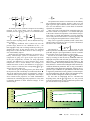
φivyiP = γ ixi fi,lpure exp
exp
Pref
P
Pref
Psat,i
P
exp
Pref
(8)
where Pref is some reference pressure, usually around 1
atm, at which pressure effects can be neglected.
Using the definition of fugacity coefficient we have:
fi, pure
P
Casting Eq. 7 into the shape shown in textbooks:
φi, pure =
46
www.aiche.org/cep/
May 2001
CEP
(11)
vil
RT
When the pressure is low and conditions are far from
the critical state, the activity coefficient is essentially independent of pressure, and it is common to set the reference
pressure to be the saturation pressure of component i,
Psat,i, and Eq. 11 is cast in the form that is usually shown
in textbooks:
P
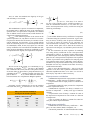
φivyiP = γ ixiPivφis exp
Pref
(9)
vi
dP
RT
(12)
For convenience in here we will set the reference pressure to 0. Eq. 11 is written as:
φivyiP = γ ixiPivφis exp –
exp
Pref
vi
dP
RT
(10)
vi
dP ×
RT
P
(7)
vi
dP
RT
φivyiP = γ ixiPivφis ×
Psat,i
0
Note that the vast majority of activity coefficient models
do not take into account their dependency on pressure,
while Eq. 6 is general and can be conveniently applied to
EOS. Thus, we recast the activity coefficient using an exact
thermodynamic relationship:
γ iP = γ iPref exp
Pref
We dropped the superscript Pref for simplicity from the
activity coefficient; its dependency on pressure is given by
the exponential term.
Using the definition of fugacity, integration up to the
saturated pure component state brings us to:
and substituting into Eq. 5 we get:
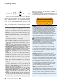
φivyiP = γ iφi,l purexiP
P
vi
dP
RT
vi
dP ×
RT
(13)
Equation 13 is mathematically equivalent to Eq. 5,
and, as long as its terms are correctly computed, it can be
used up to the critical point of the mixture (a fact sometimes brushed aside to justify the use of EOS in place of
activity-coefficient-based models). Therefore, what do
we gain in going from Eq. 5 to Eq. 13? From a physical
point of view, we gain insight into the different properties necessary to compute the phase equilibrium. From a
modeling point of view, we get two models, one for the
liquid and another for the vapor, which can be used separately (this is the counterpoint to the statement above
about activity-coefficient models — usually one does the
modeling without worrying about consistency around the
critical point).
Let us write Eq. 11 in the way normally used for
flash calculations: