Download LCModel & LCMgui User`s Manual - s

LCModel1 & LCMgui User’s
Manual
Stephen Provencher
November 8, 2015
1
LCModel Version 6.3-1L
c 1992–2015 by Stephen
LCModel, LCMgui and their documentation are copyrighted Provencher. All rights are reserved.
The latest version of the complete LCModel/LCMgui package and the documentation can be downloaded from the following site:
http://lcmodel.ca
DISCLAIMER
Please also read the License Agreement for LCModel/LCMgui, which is on
http://lcmodel.ca/lcm-license.shtml.
The sole task of LCModel is quantitation of proton MRS data, input in the standard
LCModel format. To help users, most of the LCModel manual now covers areas far
beyond this task. For example:
• Information on data acquisition, conversion and scaling for the numerous
data and hardware types is based on information kindly provided by others.
It may not be up to date, accurate or complete. Consult the manufacturer
of your hardware.
• Much additional information on possible applications is based on research,
still in progress, and subject to error and revision.
The LCModel manual (LCModel & LCMgui User’s Manual) is available free
of charge, on the understanding that neither the author, nor Stephen
Provencher Incorporated nor any contributors of information to the
LCModel manual shall be held liable for possible errors or omissions in
the LCModel manual or the consequences thereof.
2
Contents
1 Preface & Overview
11
1.1
What You Must Read . . . . . . . . . . . . . . . . . . . . . . . . . . .
11
1.2
Normal Use of LCModel . . . . . . . . . . . . . . . . . . . . . . . . . .
12
1.3
Conventions & Notation . . . . . . . . . . . . . . . . . . . . . . . . . .
12
1.3.1
Figures . . . . . . . . . . . . . . . . . . . . . . . . . . . . . . .
13
Acknowledgments . . . . . . . . . . . . . . . . . . . . . . . . . . . . . .
13
1.4
2 One-Page Output
2.1
15
Concentration Table . . . . . . . . . . . . . . . . . . . . . . . . . . . .
15
2.1.1
Upper Part . . . . . . . . . . . . . . . . . . . . . . . . . . . . .
16
2.1.2
Lower Part . . . . . . . . . . . . . . . . . . . . . . . . . . . . .
16
2.1.3
Prior Ratio Probabilities . . . . . . . . . . . . . . . . . . . . . .
17
2.2
Plot . . . . . . . . . . . . . . . . . . . . . . . . . . . . . . . . . . . . .
17
2.3
Diagnostics . . . . . . . . . . . . . . . . . . . . . . . . . . . . . . . . .
17
2.4
Miscellaneous Output . . . . . . . . . . . . . . . . . . . . . . . . . . .
18
2.5
Input Changes . . . . . . . . . . . . . . . . . . . . . . . . . . . . . . .
18
3 Essential Guide
19
3.1
Special Spectra . . . . . . . . . . . . . . . . . . . . . . . . . . . . . . .
19
3.2
Chemical Shift Imaging . . . . . . . . . . . . . . . . . . . . . . . . . .
20
3.3
Acquisition Parameters
. . . . . . . . . . . . . . . . . . . . . . . . . .
20
3.4
Analysis Window . . . . . . . . . . . . . . . . . . . . . . . . . . . . . .
21
3.4.1
PPMEND . . . . . . . . . . . . . . . . . . . . . . . . . . . . . . .
21
3.4.2
PPMST . . . . . . . . . . . . . . . . . . . . . . . . . . . . . . . .
21
Criteria for Rejecting Analyses . . . . . . . . . . . . . . . . . . . . . .
22
3.5
3
4
CONTENTS
3.6
3.7
3.5.1
Non-Random Residuals . . . . . . . . . . . . . . . . . . . . . .
22
3.5.2
Wild Baseline . . . . . . . . . . . . . . . . . . . . . . . . . . . .
22
Causes & Remedies for Failures . . . . . . . . . . . . . . . . . . . . . .
23
3.6.1
Artifacts . . . . . . . . . . . . . . . . . . . . . . . . . . . . . . .
23
3.6.2
Referencing . . . . . . . . . . . . . . . . . . . . . . . . . . . . .
23
3.6.3
Phasing . . . . . . . . . . . . . . . . . . . . . . . . . . . . . . .
23
3.6.4
Smoothing . . . . . . . . . . . . . . . . . . . . . . . . . . . . .
23
Vendor-Specific Guidelines . . . . . . . . . . . . . . . . . . . . . . . . .
24
3.7.1
Bruker . . . . . . . . . . . . . . . . . . . . . . . . . . . . . . . .
24
3.7.2
GE . . . . . . . . . . . . . . . . . . . . . . . . . . . . . . . . . .
24
3.7.3
Hitachi . . . . . . . . . . . . . . . . . . . . . . . . . . . . . . .
25
3.7.4
Marconi/Picker . . . . . . . . . . . . . . . . . . . . . . . . . . .
25
3.7.5
Bruker, Philips, Siemens, Toshiba, Varian, Microsoft . . . . . .
25
3.7.6
Philips . . . . . . . . . . . . . . . . . . . . . . . . . . . . . . . .
25
3.7.7
Siemens . . . . . . . . . . . . . . . . . . . . . . . . . . . . . . .
26
3.7.8
Toshiba . . . . . . . . . . . . . . . . . . . . . . . . . . . . . . .
26
3.7.9
Varian/Agilent . . . . . . . . . . . . . . . . . . . . . . . . . . .
27
3.7.10 Other Vendors . . . . . . . . . . . . . . . . . . . . . . . . . . .
27
4 Installation and Test Runs
28
4.1
PostScript Output . . . . . . . . . . . . . . . . . . . . . . . . . . . . .
28
4.2
Test Runs Using LCMgui . . . . . . . . . . . . . . . . . . . . . . . . .
28
4.2.1
Display on Your Screen . . . . . . . . . . . . . . . . . . . . . .
28
4.2.2
PostScript Printer . . . . . . . . . . . . . . . . . . . . . . . . .
29
4.2.3
No Printer or Display . . . . . . . . . . . . . . . . . . . . . . .
30
4.2.4
Further Tests . . . . . . . . . . . . . . . . . . . . . . . . . . . .
30
4.2.5
More Complete Test of LCMgui with a False License . . . . . .
30
4.2.6
Starting Over . . . . . . . . . . . . . . . . . . . . . . . . . . . .
31
4.3
Test Runs without LCMgui . . . . . . . . . . . . . . . . . . . . . . . .
31
4.4
Benchmark Timings . . . . . . . . . . . . . . . . . . . . . . . . . . . .
32
CONTENTS
5
5 Running LCModel without LCMgui – Basic Input
5.1
5.2
5.3
33
Conventions . . . . . . . . . . . . . . . . . . . . . . . . . . . . . . . . .
33
5.1.1
File extensions . . . . . . . . . . . . . . . . . . . . . . . . . . .
33
5.1.2
Control Parameter Conventions . . . . . . . . . . . . . . . . . .
34
.RAW File . . . . . . . . . . . . . . . . . . . . . . . . . . . . . . . . . .
34
5.2.1
Namelist SEQPAR . . . . . . . . . . . . . . . . . . . . . . . . . .
35
5.2.2
Namelist NMID . . . . . . . . . . . . . . . . . . . . . . . . . . .
35
5.2.3
Time-Domain Data . . . . . . . . . . . . . . . . . . . . . . . . .
36
.CONTROL File . . . . . . . . . . . . . . . . . . . . . . . . . . . . . . . .
37
5.3.1
Instrument and Acquisition . . . . . . . . . . . . . . . . . . . .
38
5.3.2
Multi-Voxel Data Sets . . . . . . . . . . . . . . . . . . . . . . .
38
5.3.3
Analysis Window . . . . . . . . . . . . . . . . . . . . . . . . . .
39
5.3.4
Eddy-Current Correction . . . . . . . . . . . . . . . . . . . . .
40
5.3.5
First-Order Phase Correction . . . . . . . . . . . . . . . . . . .
41
5.3.6
PostScript Output . . . . . . . . . . . . . . . . . . . . . . . . .
41
5.3.7
Archiving the Results . . . . . . . . . . . . . . . . . . . . . . .
42
5.3.8
Phantoms . . . . . . . . . . . . . . . . . . . . . . . . . . . . . .
43
6 Elementary Guide to LCMgui
44
6.1
Starting LCMgui . . . . . . . . . . . . . . . . . . . . . . . . . . . . . .
44
6.2
Selecting the Data to be Analyzed . . . . . . . . . . . . . . . . . . . .
44
6.2.1
File Selector Window . . . . . . . . . . . . . . . . . . . . . . .
45
Control Parameters Window . . . . . . . . . . . . . . . . . . . . . . . .
46
6.3.1
Analyzing spectrum from: . . . . . . . . . . . . . . . . . . . . .
47
6.3.2
BASIS file: . . . . . . . . . . . . . . . . . . . . . . . . . . . . .
47
6.3.3
Do eddy-current correction . . . . . . . . . . . . . . . . . . . .
48
6.3.4
Do water-scaling . . . . . . . . . . . . . . . . . . . . . . . . . .
48
6.3.5
Only for Multi-Voxel data files: . . . . . . . . . . . . . . . . . .
49
6.3.6
The Rest of the Control Parameters Window . . . . . . . . . .
49
6.3.7
Reload Data . . . . . . . . . . . . . . . . . . . . . . . . . . . .
49
6.4
Run LCModel . . . . . . . . . . . . . . . . . . . . . . . . . . . . . . . .
50
6.5
Where is the Output? . . . . . . . . . . . . . . . . . . . . . . . . . . .
51
6.3
6
CONTENTS
6.6
Interactive Processing with LCMgui . . . . . . . . . . . . . . . . . . .
51
6.7
Getting out of LCMgui . . . . . . . . . . . . . . . . . . . . . . . . . . .
51
7 LCMgui Reference Manual
7.1
7.2
7.3
7.4
7.5
53
LCMgui Structure . . . . . . . . . . . . . . . . . . . . . . . . . . . . .
53
7.1.1
Limitations . . . . . . . . . . . . . . . . . . . . . . . . . . . . .
54
Installing LCMgui . . . . . . . . . . . . . . . . . . . . . . . . . . . . .
54
7.2.1
Multi-User Installations . . . . . . . . . . . . . . . . . . . . . .
54
7.2.2
Starting LCMgui . . . . . . . . . . . . . . . . . . . . . . . . . .
55
7.2.3
First Test Runs . . . . . . . . . . . . . . . . . . . . . . . . . . .
55
7.2.4
Install Model Spectra . . . . . . . . . . . . . . . . . . . . . . .
55
7.2.5
Install License . . . . . . . . . . . . . . . . . . . . . . . . . . .
56
7.2.6
Installing Updates & Upgrades . . . . . . . . . . . . . . . . . .
57
Basic Settings and Usage . . . . . . . . . . . . . . . . . . . . . . . . .
58
7.3.1
Vendor-Specific Guidelines . . . . . . . . . . . . . . . . . . . . .
58
7.3.2
.BASIS file . . . . . . . . . . . . . . . . . . . . . . . . . . . . .
60
7.3.3
Archiving the LCModel Results . . . . . . . . . . . . . . . . . .
60
7.3.4
View/Edit Control Parameters . . . . . . . . . . . . . . . . . .
63
7.3.5
Saving Your Control Parameters . . . . . . . . . . . . . . . . .
65
7.3.6
Changing your Default Control Parameters . . . . . . . . . . .
67
7.3.7
User Profiles . . . . . . . . . . . . . . . . . . . . . . . . . . . .
68
Further Useful Settings . . . . . . . . . . . . . . . . . . . . . . . . . . .
69
7.4.1
Previewing Data . . . . . . . . . . . . . . . . . . . . . . . . . .
69
7.4.2
Interactive Processing . . . . . . . . . . . . . . . . . . . . . . .
71
7.4.3
Execution Scripts . . . . . . . . . . . . . . . . . . . . . . . . . .
71
7.4.4
Processing Non-Standard Data Files . . . . . . . . . . . . . . .
72
7.4.5
Optional Preprocessor . . . . . . . . . . . . . . . . . . . . . . .
73
7.4.6
Changing the License & the Print Command . . . . . . . . . .
74
Fine Points . . . . . . . . . . . . . . . . . . . . . . . . . . . . . . . . .
75
7.5.1
gui-defaults Resource File . . . . . . . . . . . . . . . . . . .
75
7.5.2
Cleaning up the File System
77
. . . . . . . . . . . . . . . . . . .
CONTENTS
7
8 Making the Basis Set
78
8.1
Compatibility Requirements . . . . . . . . . . . . . . . . . . . . . . . .
78
8.2
Model Metabolite Solutions . . . . . . . . . . . . . . . . . . . . . . . .
79
8.2.1
Choice of Model Metabolites . . . . . . . . . . . . . . . . . . .
79
8.2.2
Reference Markers . . . . . . . . . . . . . . . . . . . . . . . . .
80
8.2.3
Phantom . . . . . . . . . . . . . . . . . . . . . . . . . . . . . .
82
8.2.4
Solutions . . . . . . . . . . . . . . . . . . . . . . . . . . . . . .
82
Acquiring the Basis Spectra . . . . . . . . . . . . . . . . . . . . . . . .
83
8.3.1
Quality . . . . . . . . . . . . . . . . . . . . . . . . . . . . . . .
83
8.3.2
Consistency . . . . . . . . . . . . . . . . . . . . . . . . . . . . .
83
8.3.3
Acquisition Time and Bandwidth . . . . . . . . . . . . . . . . .
84
8.3.4
Repetition Time . . . . . . . . . . . . . . . . . . . . . . . . . .
84
Eddy-Current Correction . . . . . . . . . . . . . . . . . . . . . . . . .
84
8.4.1
ECC with LCMgui . . . . . . . . . . . . . . . . . . . . . . . . .
85
8.4.2
ECC without LCMgui . . . . . . . . . . . . . . . . . . . . . . .
86
Plotting .RAW Files with PlotRaw . . . . . . . . . . . . . . . . . . . . .
87
8.5.1
Test Run of PlotRaw . . . . . . . . . . . . . . . . . . . . . . . .
87
8.5.2
PlotRaw .IN File . . . . . . . . . . . . . . . . . . . . . . . . . .
87
8.5.3
PlotRaw Diagnostics . . . . . . . . . . . . . . . . . . . . . . . .
89
Running MakeBasis . . . . . . . . . . . . . . . . . . . . . . . . . . . .
90
8.6.1
Auto-Scaling . . . . . . . . . . . . . . . . . . . . . . . . . . . .
91
8.6.2
Judging the Basis Spectra . . . . . . . . . . . . . . . . . . . . .
91
8.6.3
.RAW File . . . . . . . . . . . . . . . . . . . . . . . . . . . . . .
91
8.6.4
MakeBasis .IN File . . . . . . . . . . . . . . . . . . . . . . . . .
92
8.6.5
MEGA-PRESS . . . . . . . . . . . . . . . . . . . . . . . . . . .
96
8.6.6
MakeBasis Diagnostics . . . . . . . . . . . . . . . . . . . . . . .
96
8.6.7
Output .BASIS File . . . . . . . . . . . . . . . . . . . . . . . .
98
Calibrating Basis Spectra . . . . . . . . . . . . . . . . . . . . . . . . .
98
8.7.1
Calibrating GPC/PCh & NAA/NAAG
98
8.7.2
Adding New Basis Spectra . . . . . . . . . . . . . . . . . . . . 100
8.3
8.4
8.5
8.6
8.7
8.8
. . . . . . . . . . . . .
Summary . . . . . . . . . . . . . . . . . . . . . . . . . . . . . . . . . . 101
8
CONTENTS
9 Further Useful Options and Information
102
9.1
Special Types of Spectra . . . . . . . . . . . . . . . . . . . . . . . . . . 102
9.2
Muscle Spectra . . . . . . . . . . . . . . . . . . . . . . . . . . . . . . . 103
9.3
9.4
9.2.1
Standard Input . . . . . . . . . . . . . . . . . . . . . . . . . . . 103
9.2.2
Additional Input . . . . . . . . . . . . . . . . . . . . . . . . . . 104
9.2.3
Output . . . . . . . . . . . . . . . . . . . . . . . . . . . . . . . 105
Lipid Spectra (Liver, Breast, Bone, etc.) . . . . . . . . . . . . . . . . . 106
9.3.1
Input . . . . . . . . . . . . . . . . . . . . . . . . . . . . . . . . 107
9.3.2
Output . . . . . . . . . . . . . . . . . . . . . . . . . . . . . . . 109
9.3.3
Estimating only choline . . . . . . . . . . . . . . . . . . . . . . 110
MEGA-PRESS for GABA . . . . . . . . . . . . . . . . . . . . . . . . . 111
9.4.1
Input . . . . . . . . . . . . . . . . . . . . . . . . . . . . . . . . 111
9.4.2
Output . . . . . . . . . . . . . . . . . . . . . . . . . . . . . . . 114
9.5
Internal Logical Units . . . . . . . . . . . . . . . . . . . . . . . . . . . 114
9.6
Eddy-Current Correction . . . . . . . . . . . . . . . . . . . . . . . . . 115
9.7
Prior Phasing Information . . . . . . . . . . . . . . . . . . . . . . . . . 115
9.7.1
9.8
9.9
Estimating Appropriate SDDEGZ, SDDEGP, DEGZER & DEGPPM . 116
Specifying the Basis Spectra for the Analysis . . . . . . . . . . . . . . 117
9.8.1
Omitting Basis Spectra from the Analysis . . . . . . . . . . . . 117
9.8.2
Keeping Basis Spectra in the Analysis . . . . . . . . . . . . . . 117
One-Page Output . . . . . . . . . . . . . . . . . . . . . . . . . . . . . . 118
9.9.1
Concentration Table . . . . . . . . . . . . . . . . . . . . . . . . 118
9.9.2
Diagnostics Table . . . . . . . . . . . . . . . . . . . . . . . . . . 120
9.9.3
Plot . . . . . . . . . . . . . . . . . . . . . . . . . . . . . . . . . 120
9.9.4
Miscellaneous Output Table . . . . . . . . . . . . . . . . . . . . 122
10 Absolute Metabolite Concentrations
124
10.1 Calibration Phantoms . . . . . . . . . . . . . . . . . . . . . . . . . . . 125
10.1.1 Data Scaling (intra-hardware) . . . . . . . . . . . . . . . . . . . 125
10.1.2 Scanner Calibration (inter-hardware) . . . . . . . . . . . . . . . 127
10.2 Water-Scaling . . . . . . . . . . . . . . . . . . . . . . . . . . . . . . . . 128
10.2.1 Method . . . . . . . . . . . . . . . . . . . . . . . . . . . . . . . 128
CONTENTS
9
10.2.2 Usage . . . . . . . . . . . . . . . . . . . . . . . . . . . . . . . . 128
11 Fine Points
132
11.1 Error Estimates & Reproducibility . . . . . . . . . . . . . . . . . . . . 132
11.1.1 Averaging Concentrations over a Series of Analyses . . . . . . . 133
11.2 Relaxation Corrections . . . . . . . . . . . . . . . . . . . . . . . . . . . 133
11.3 Prior Referencing Information . . . . . . . . . . . . . . . . . . . . . . . 134
11.3.1 Off-Resonance Spectra . . . . . . . . . . . . . . . . . . . . . . . 134
11.3.2 Referencing to Water . . . . . . . . . . . . . . . . . . . . . . . . 135
11.3.3 Inputting a Starting Shift . . . . . . . . . . . . . . . . . . . . . 135
11.3.4 Fixing the Shift . . . . . . . . . . . . . . . . . . . . . . . . . . . 136
11.3.5 Details of Automated Referencing . . . . . . . . . . . . . . . . 136
11.4 Multi-Voxel Data Sets . . . . . . . . . . . . . . . . . . . . . . . . . . . 137
11.4.1 GE CSI data . . . . . . . . . . . . . . . . . . . . . . . . . . . . 137
11.4.2 Non-GE CSI data . . . . . . . . . . . . . . . . . . . . . . . . . 137
11.4.3 Multi-Voxel Filenames . . . . . . . . . . . . . . . . . . . . . . . 138
11.4.4 Output for spreadsheets . . . . . . . . . . . . . . . . . . . . . . 139
11.4.5 Combining Multi-Voxel .PS files . . . . . . . . . . . . . . . . . 139
11.4.6 Skipping bad voxels . . . . . . . . . . . . . . . . . . . . . . . . 139
11.5 Basis Spectra in the Preliminary Analysis . . . . . . . . . . . . . . . . 140
11.6 Unusual Phantoms . . . . . . . . . . . . . . . . . . . . . . . . . . . . . 140
11.7 Simulating Basis Spectra . . . . . . . . . . . . . . . . . . . . . . . . . . 140
11.7.1 Method . . . . . . . . . . . . . . . . . . . . . . . . . . . . . . . 142
11.8 Concentration Ratio Priors . . . . . . . . . . . . . . . . . . . . . . . . 143
11.8.1 Omitting Ratio Priors . . . . . . . . . . . . . . . . . . . . . . . 145
11.9 Coherent Data Averaging . . . . . . . . . . . . . . . . . . . . . . . . . 145
11.9.1 GE & Toshiba Phased-Array Single-Voxel Data . . . . . . . . . 145
11.9.2 Other Spectra with Identical Phases & Referencing Shift . . . . 146
11.9.3 Varying Phases or Referencing Shifts . . . . . . . . . . . . . . . 146
11.10 Analyzing a (Time) Series of Spectra . . . . . . . . . . . . . . . . . . 147
11.11 Analyzing Data Left & Right of the Water Signal . . . . . . . . . . . 147
11.12 Multimodal Lineshapes . . . . . . . . . . . . . . . . . . . . . . . . . . 148
10
CONTENTS
11.13 Relaxation & Shift Priors . . . . . . . . . . . . . . . . . . . . . . . . . 148
11.14 Detailed Output . . . . . . . . . . . . . . . . . . . . . . . . . . . . . . 149
11.15 Default Control Parameters . . . . . . . . . . . . . . . . . . . . . . . . 150
11.16 Analyzing Magnitude Spectra . . . . . . . . . . . . . . . . . . . . . . 151
11.17 Consistency with Old Versions . . . . . . . . . . . . . . . . . . . . . . 151
11.18 Nuclei Other than 1 H . . . . . . . . . . . . . . . . . . . . . . . . . . . 152
12 Diagnostics and Troubleshooting Hints
153
12.1 Non-Standard Diagnostics . . . . . . . . . . . . . . . . . . . . . . . . . 153
12.1.1 I/O Errors . . . . . . . . . . . . . . . . . . . . . . . . . . . . . 153
12.1.2 Arithmetic Exceptions . . . . . . . . . . . . . . . . . . . . . . . 154
12.1.3 Other Aborts with no One-Page Output . . . . . . . . . . . . . 154
12.2 Standard LCModel Diagnostics . . . . . . . . . . . . . . . . . . . . . . 154
Chapter 1
Preface & Overview
The LCModel package is for the automatic quantitation of in vivo proton MR spectra [1]. LCMgui is a graphical user interface for running LCModel with more convenience and less knowledge of this manual. LCMgui is provided without charge for
use with LCModel only.
1.1
What You Must Read
In order to avoid the proliferation of documents, this is the only manual for the
LCModel package and LCMgui. It is a detailed reference manual. However, as
outlined below, most of you can use this as a shorter users guide, consisting of only
a few of the chapters here. In addition, some parts are clearly noted to be only of
interest to users of LCMgui and many parts only to non-users.
The only necessary reading for everyone is the Disclaimer on page 2 and
Chaps. 1–3. LCMgui users will also find Chapter 6 useful. It is also assumed throughout this manual that you are familiar with Ref. [1] (but not necessarily its Appendix).
This is sufficient for most users (referred to here as Normal Users); it should allow
you to competently use LCModel.
Chapters 4 & 5 need only be read by the person initially installing LCModel in
your laboratory. Chapter 5 describes important input Control Parameters specific to
your spectra, such as field strength, dwell time, etc. With LCMgui, these are often
automatically determined.
Chapter 6 is a guide on the basics of using LCMgui. It is highly recommended for
LCMgui users.
Chapter 7 is a detailed reference manual on LCMgui. It can help you fully exploit
the flexibility of LCMgui and optimally install and configure it for your site and your
Normal Users.
Chapter 8 need only be read by the person constructing the Basis Set of in vitro
model metabolite Basis Spectra for your laboratory. This is not necessary if your
sequence matches one of the Basis Sets that are freely available; check with me first.
11
12
CHAPTER 1. PREFACE & OVERVIEW
Chapter 9 describes further useful Control Parameters.
Chapter 10 need only be read if you want to estimate absolute metabolite concentrations; it is not necessary for concentration ratios.
Chapter 11 discusses fine points and further Control Parameters that will be useful
for some users.
Chapter 12 explains all of LCModel’s diagnostic messages and gives general hints for
troubleshooting.
Even as a lowly Normal User, you may still want to at least look at the Table of
Contents at the front of this manual to get an overview of all the possibilities of
LCModel. It is easy to modify the LCModel Control Parameters to make use of the
possibilities described in Chaps. 5, 9 & 11.
LCMgui users may also want to learn about a Control Parameter or other term that
is usually set automatically for them. You can often look up such a term using the
Index at the end of this manual.
1.2
Normal Use of LCModel
With LCMgui, you generally only have to click on a few choices, such as the name
of the file containing the data to be analyzed.
Instead of using LCMgui, the person installing LCModel could also write a simple
Pre-Formatting Program or script to automatically format the input data and then
run LCModel. Then the Normal User only has to input the name of the raw timedomain data to be analyzed.
It is not even necessary to view the data before analysis; phasing, referencing, and
quantitation are done automatically by LCModel. There is also another LCModel
output file archiving the results, which are then available for computing means, standard deviations, trends, etc., in the metabolite concentrations in a series of measurements. Since there is no user interaction, the results are user-independent, thus
improving objectivity and exchangeability of the results within and between laboratories.
1.3
Conventions & Notation
Metabolite abbreviations are used throughout and are defined in Table 8.1.
As already used above, [1] means reference [1] in the Bibliography at the end of this
manual.
Special terms, such as Normal User, are italicized the first time that they appear and
capitalized thereafter. Less obvious special terms are in the Index at the end of this
manual, and are therefore not cross-referenced when they appear in the text.
1.4. ACKNOWLEDGMENTS
13
File names and LCModel input/output are written in the teletype style, as figures.pdf.
Your home directory is specified by $HOME/, although you can usually abbreviate this
with a tilde, ∼ /.
Unix means Sun, SGI or Compaq/DEC, in the few cases where they behave differently
from the Linux version.
Concentrations should be labeled “mmol per Kg wet weight”. We use the shorter (incorrect) abbreviation mM. The actual mM is the mmol per Kg wet weight multiplied
by the specific gravity of the tissue, typically 1.04 in brain.
We use the term “directory” and not “folder”.
Further conventions for more advanced users are defined in Sec 5.1.
1.3.1
Figures
Figure 6.2 or Fig 6.2 refers to Fig 6.2 in Chap 6 of this manual.
PLOT 6 (PLOT rather than Figure and no decimal point in the number) is not in
this manual; it is in the file $HOME/.lcmodel/doc/figures.pdf. You should output
this on a printer with PostScript capability, as was done with this manual (which is
in the same directory) . It is convenient to have these figures bound separately from
this manual, so that the two can be read side-by-side.
[1, Fig 2] means Fig 2 in Ref. [1].
1.4
Acknowledgments
I thank the Biomedizinische NMR Group in Göttingen, especially Wolfgang Hänicke,
for providing much data during the development of LCModel. The first 10,000 spectra
were processed with LCModel by them [2]. I thank Jens Frahm for permission to use
the test data in this manual.
I am very grateful to many other users of LCModel for helpful comments, which have
significantly contributed to the development of LCModel.
I thank the groups at GE Medical Systems, Toshiba Medical Systems, Marconi,
Bruker Medical, Varian, Philips and Siemens Medical Solutions for providing much
information on their data structures. I am especially grateful to Rolf Schulte (Munich) for guidance and GAMMA routines for simulating model metabolite spectra,
to Jim Murdoch (Cleveland) for detailed information on Picker and Philips data conversion and to JBob Brown (Fremont) and Timo Schirmer (Munich) for essential
information on GE data conversion.
I thank the GE, Marconi, and Bruker groups and Else Danielsen (Copenhagen),
Thomas Michaelis (Göttingen) and Petra Pouwels (Amsterdam), Jan Weis (Uppsala), Noriaki Hattori (Osaka), and R. Mark Wellard (Brisbane) for providing model
spectra, and Xiangling Mao (Göttingen) for information on Siemens data. Section
8.2 is mainly based on the results of Thomas Michaelis and Petra Pouwels.
14
CHAPTER 1. PREFACE & OVERVIEW
The code generating the PostScript output files is based on advice and routines kindly
provided by Christian Labadie, Dept. of Chemistry, SUNY Stony Brook.
I am grateful to Gunther Helms (Tübingen), Else R. Danielsen (Copenhagen), Markus
Wick (Ettlingen), Uwe Seeger (Tübingen) and Jens Frahm (Göttingen) for information and suggestions on scaling for absolute concentrations. I thank Uwe Seeger also
for making [3] available before publication and for helpful discussions on including
lipids and macromolecules in the analysis. I thank Brad Beyenhof for advice on forwarding X windows. I thank Philipp Böhm-Sturm (Berlin) for much information and
advice on Bruker data.
LCMgui was written with the free software packages
Tcl/Tk, http://www.tcl.tk,
Tix (Ioi K. Lam, http://tixlibrary.sourceforge.net) and
Plus Patches (Jan Nijtmans, http://members1.chello.nl/∼j.nijtmans/plus.html).
Chapter 2
One-Page Output
The results of an LCModel analysis are summarized on the so-called One-Page Output
(now usually two pages), contained in a PostScript file. Print out
$HOME/.lcmodel/doc/figures.pdf. PLOTs 1 & 2 there show the One-Page Output
from an analysis of the test data supplied with your LCModel package.
At the top is the title. Normally LCMgui or another Pre-Formatting Program automatically supplies this by copying identification information from a header in the
original data file.
2.1
Concentration Table
These are the results of main interest to you. The most important message of this
chapter is that, before looking at the concentrations themselves, you should always
look first at the entries in the %SD column. These are the estimated standard deviations (Cramér-Rao lower bounds) expressed in percent of the estimated concentrations. These %SD estimates are only lower bounds (Sec 11.1), but they are still
the most useful reliability indicators. As usual, you must multiply them by 2.0 to
get rough 95% confidence intervals; i.e., the range that would contain the true value
about 95% of the time. Thus:
• %SD > 50% indicates that the metabolite concentration could well range from
zero to twice the estimated concentration. Thus, the metabolite is practically
undetectable with this data. Several metabolites are often undetectable in
normal subjects.
• %SD ≈ 20% indicates that only changes of about 40% can be detected with
reliability, e.g., the approximate doubling of Gln/Glu in several pathologies. A
%SD < 20% has been used by many as a very rough criterion for estimates of
acceptable reliability. However, it is only a subjective indication, not a rigorous
limit.
• %SD < 15% are in boldface blue.
• Of course, averages over a group of LCModel analyses of similar spectra can
significantly reduce the uncertainties. Section 11.1.1 specifies how to compute
these average concentrations.
15
16
CHAPTER 2. ONE-PAGE OUTPUT
The abbreviations of the metabolites are in the 4th column. (Table 8.1 defines most
of these Metabolite Names.) The corresponding absolute concentrations are in the
1st column. Usually the units of the absolute concentrations are unknown, and only
concentration ratios are meaningful. These ratios are given in the 3rd column, whose
heading (/Cr) indicates that the ratio is relative to creatine (plus phosphocreatine).
Only when the Basis Spectra and your input data are consistently scaled with each
other, are the absolute concentrations meaningful; for example, you can use WaterScaling (Sec 6.3.4 & Chap 10).
2.1.1
Upper Part
The Concentration Table usually is split into two parts by a horizontal line. The
upper part contains the usual low molecular weight metabolites of interest.
NAAG is quite difficult to resolve from NAA, and PCh is very difficult to resolve
from GPC, as is PCr from Cr. With lower quality spectra (or long TE), Glu and
Gln are also often difficult to resolve. The last three rows of the upper part of the
table are the sums of these concentration pairs. The sum GPC+PCh is much more
accurate than the individual concentrations, as can be clearly seen from the much
lower %SD for GPC+PCh than for GPC and PCh.
-CrCH2 is a correction term, rather than a metabolite of interest. It is a simulated
negative creatine CH2 singlet around 3.94 ppm. This corrects for attenuation of the
Cr CH2 singlet due to water suppression and differential relaxation effects at longer
TE.
Gua is a simulated singlet to account for occasional significant signals at 3.78 ppm,
especially in tumors. The Gua stood for guanidinoacetate [4], but, in nearly all cases,
this assignment is probably wrong, and Gua is only an empirical fit to the signal at
3.78 ppm (which may be partly due to GSH).
2.1.2
Lower Part
The lower part of the Concentration Table contains simulated lipid (Lip) and macromolecule (MM) components. As with -CrCH2, they are often considered nuisance
correction parameters, but they may also be of interest, e.g., in classifying tumors
[5].
Section 11.7 defines the Metabolite Names in this lower part. It also explains how
to specify your own simulated components. The numbers after MM (for “macromolecules”) and Lip (for “lipids”) indicate the approximate chemical shift in ppm
of the peaks; e.g., MM14 for the macromolecule peak near 1.4 ppm (which may also
contain lipid contributions).
If Water-Scaling (Sec 6.3.4) is used to estimate the concentrations in the upper part
in mM; then all of the MM* & Lip* will be in mM of CH2 groups, except for Lip09
& MM09, which will be in mM of CH3 groups. Otherwise, the (unknown) scaling
of the simulated metabolites will be inconsistent with the (unknown) scaling of the
metabolites in the Basis Set.
2.2. PLOT
2.1.3
17
Prior Ratio Probabilities
Section 11.8 shows how prior probabilities (so-called “soft constraints”) are imposed
on ratios of some poorly determined concentrations to more accurate concentrations.
An example is Lip09/Lip13a+Lip13b, the ratio of the lipids near 0.9 ppm to those
near 1.3 ppm. In PLOT 1 in $HOME/.lcmodel/doc/figures.pdf, the line with
Lip09 is bold-italic red and the name Lip09 is preceded by a minus sign. This
means that the Lip09 concentration is significantly lower than expected. (A plus
would mean significantly higher.) This is common with the highly variable lipids and
macromolecules.
There are similar (very weak) constraints on the weak normal metabolites Asp,
GABA, Glc, Scyllo and Tau. If one of these is output in red italic, then consider
whether this may be a real effect due to a pathology. If so, then use Sec 11.8.1 to
omit this constraint.
2.2
Plot
The real part of the frequency-domain data (spectrum; i.e., the phased and referenced
FFT of your raw input data with no smoothing) is plotted as a thin curve. The thick
red curve is the LCModel fit to this data. Also plotted as a thin curve is the so-called
Baseline. We will call the ppm-range of the plot the Analysis Window (i.e., the range
over which the data are analyzed).
At the top are plotted the Residuals, i.e., the data minus the fit to the data. The
Residuals are a sensitive diagnostic of the analysis. In PLOT 1 in
$HOME/.lcmodel/doc/figures.pdf, they look fairly randomly scattered about zero,
indicating a fit to within experimental error, with no apparent systematic errors.
Section 3.5 gives a series of examples and guidelines on the diagnostic use of the
Residuals and Baseline.
2.3
Diagnostics
The table below the Concentration Table summarizes all the diagnostic messages
from LCModel during this analysis. Always look at this table. The 5 types of
diagnostics, in increasing order of severity, are: info, warning (boldface blue), and
(all in boldface red) ERROR, FATAL and ILLOGICAL. Chapter 12 lists and explains
each diagnostic and suggests possible remedies. You should consult Chap 12 if ERROR
or warning occurs. The type info is generally harmless.
When FATAL or ILLOGICAL occurs, the run aborts, and you must consult Chap 12.
If the run aborts, whatever is available is plotted —
• the usual fit to the data (usually not available), or
• the absolute value of the frequency-domain data (the Absolute-Value Plot), or
• no plots, only the tables of diagnostics and input changes (if the raw data have
not yet been read in).
18
CHAPTER 2. ONE-PAGE OUTPUT
The Absolute-Value Plot (of the test data) is illustrated in PLOT 5 in
$HOME/.lcmodel/doc/figures.pdf, where the FATAL was caused by inputting unreasonable values for a Control Parameter (DOREFS). The most common causes of a
FATAL are input errors (which are usually obvious from the diagnostics) or hopelessly
bad data (which is often immediately apparent from the Absolute-Value Plot).
2.4
Miscellaneous Output
The lines in this table are:
(1) FWHM (full width at half-maximum) is a rough estimate of the linewidth in
the in vivo spectrum.
S/N is defined here as the ratio of the maximum in the spectrum-minusBaseline over the Analysis Window to twice the rms Residuals. This seems
to be widely used [6, p. 218], but some may use twice this value. This S/N is
also rough, because it depends on offsets in the model spectra and Baseline.
Neither of these single numbers can unambiguously characterize the quality
of your data. They are only rough guides. Only the %SD values in the
Concentration Table simultaneously account for both resolution and noise
level (as well as many other things) to give the most useful guides to the
reliability of the estimates.
(2) Data shift: the referencing shift performed on the data spectrum.
(3) Ph: the zero-order and first-order data phase corrections, φ0 and φ1 , using
the conventions in the definition of DEGPPM in Sec 8.5.2.
Section 9.9.4 explains optional additional output that you can easily get in this table.
2.5
Input Changes
This last table lists all input that was made to change default Control Parameters in LCModel. These are usually automatically supplied by LCMgui or the PreFormatting Program to set Control Parameters characteristic of your instrument. If
the list is too long to fit on the front page, then, by default, a second page (PLOT 2
in $HOME/.lcmodel/doc/figures.pdf) with all the tables is printed. It is best to
use a printer that prints on both sides of a page; otherwise Sec 5.3.6 shows how to
easily suppress this second page (but then the documentation will be incomplete).
The first three lines of this table in show the simple changes (described in Sec 9.9.3.1)
to get additional plots of the individual contributions of NAA and NAAG to the
spectrum. These are shown in PLOTs 3 & 4.
Chapter 3
Essential Guide
This chapter briefly lists important guidelines and special cases. It refers you to other
chapters for details.
Print out $HOME/.lcmodel/doc/figures.pdf. Remember, figures located only in
figures.pdf are denoted by PLOT, e.g., PLOT 6. Figures located in this manual
are denoted by Figure or Fig, e.g., Fig 6.2.
3.1
Special Spectra
LCModel attempts to automatically handle a wide variety of spectra with no special
input from you, especially if you use LCMgui. However, there are some special cases
where you should input extra information to LCModel.
You input this information with Control Parameters (Sec 5.1.2). With LCMgui,
these are simply entered in the “Control Parameters” window (Fig 7.7). Without
LCMgui, they are input in Namelists (Sec 5.2.1). Many Control Parameters have
default values, but you override these defaults when you input values yourself.
The Control Parameter SPTYPE (Sec 9.1) informs LCModel of special types of spectra
(remember that PLOTs are in $HOME/.lcmodel/doc/figures.pdf):
• Weak NAA, Tumors, Lesions: Input SPTYPE = ’tumor’ when you
suspect that the NAA singlet around 2.0 ppm could be weak compared to
the cholines (around 3.2 ppm) or the creatines or the lipid or macromolecule
signals around 1.3 or 0.9 ppm. So, this is not only for tumors.
See PLOTs 6 & 7 in $HOME/.lcmodel/doc/figures.pdf for examples and
Sec 9.1 for instructions.
• Muscle: Input SPTYPE = ’muscle-5’ for muscle spectra. See PLOT 8
for an example and Sec 9.2 for important limitations and instructions.
• Lipids, Breast, Liver, etc.: For spectra with mainly lipids (and water)
and possibly choline. Examples are in PLOTs 9–11. To use these, you
must read Sec 9.3.
19
20
CHAPTER 3. ESSENTIAL GUIDE
• MEGA-PRESS: Input SPTYPE = ’mega-press-3’ for quantifying GABA
[7] using MEGA-PRESS. To use this, you must read Sec 9.4.
• CSF; NAA, cholines & Cr all weak: Input SPTYPE = ’csf’ in the
(unusual) case that you have mainly cerebrospinal fluid (CSF), with the
three usual landmarks (NAA, cholines and creatines) weaker than Lac &
Glc. PLOT 13 shows an example.
3.2
Chemical Shift Imaging
For GE CSI data sets, use the Research Version of SAGE, which now has Mary
McLean’s LCModel interface [9]. For this SAGE/LCModel interface, you must use
Sec 11.4.1.
Most other 2D & 3D CSI data sets can be handled by LCMgui. (See Secs. 3.7 &
11.4.) PLOT 14 in $HOME/.lcmodel/doc/figures.pdf shows an LCMgui absolutevalue display of a full slice with 8×8 voxels. (A laser printer can usually give useful
plots of up to 32×32 voxels.)
With LCMgui, you can then select and display a rectangular subset of the voxels in
this slice and have LCModel analyze this subset (or the whole slice) in one multivoxel run. An advantage of this is that LCModel first analyzes a central voxel of the
subset and then works outwards, using Bayesian learning to get starting estimates
and “soft constraints” for the first-order phase correction and the referencing shift
from the preceding (often better) central voxels for the (often poorer) outer voxels.
This speeds up and improves the analyses.
LCModel outputs concentrations from all voxels in the subset to a file that can be
imported into spreadsheet programs (Sec 11.4.4).
You should still be selective with your subset. It is a waste of time to include outer
rows or columns with only poor spectra. Analyses of poor quality voxels can take
several times longer than normal voxels.
3.3
Acquisition Parameters
• Apodization: Never apodize the spectral data; it distorts the data and
ruins the statistical tests in LCModel. (See Sec 3.6.4.)
• AQ, the acquisition time for one scan should be long enough so that
the data always decay into the noise. At 1.5T use AQ ≥ 800 ms. At higher
fields, it is usually shorter. Consistently use the same AQ for all data with
a given sequence.
• Bandwidth should be at least 1000 Hz at 1.5T, 2000 Hz at 3T and proportional to these at other field strengths.
3.4. ANALYSIS WINDOW
3.4
21
Analysis Window
Two of the most important Control Parameters define the Analysis Window (the
window of frequency-domain data that will be analyzed). The left edge of the window
is PPMST ppm (4.0 by default). The right edge is PPMEND ppm (normally, 0.2 by
default).
3.4.1
PPMEND
Normally, you should leave PPMEND at its default of 0.2. However, there are two
important cases when this default should be changed:
(1) long echo times: When LCMgui or LCModel detects T E > 100 ms,
it resets the default to PPMEND = 1.0, because the macromolecule signal
around 0.9 ppm is usually too attenuated to be useful at such long T E.
You can override this default by inputting your own PPMEND.
(2) CSI data with lipid artifacts: Strong lipid signals often occur in voxels
near the edge of the slice. This is no problem if the lipid signals are where
they should be, around 1.3 & 0.9 ppm, as in PLOT 6 in
$HOME/.lcmodel/doc/figures.pdf. The problem is that some of these
signals can originate from outside the voxel and can be significantly shifted
or out of phase. These artifacts distort the analysis in PLOT 15. With such
artifacts, there is no hope of estimating Lac, Ala or anything else below
1.8 ppm. PLOT 16 is the analysis of the same voxel with PPMEND = 1.8.
In this particular case the concentration ratios do not change drastically,
but they can be unreliable in cases like PLOT 15. In these cases, you
should input
PPMEND = 1.8
For brain, never set PPMEND < 0.1. The model metabolite spectra usually have a DSS
marker around 0.0 ppm that must be kept out of the analysis.
For brain, PPMEND should never exceed 1.9.
3.4.2
PPMST
PPMST = 4.0 seldom has to be changed. Only when the noise is much higher in
the region near 4.0 ppm, would a lower PPMST be called for. If this would require a
PPMST < 3.85, then reject the spectrum or try omitting eddy-current correction.
LCModel attempts to find the smoothest Baseline that is still consistent with the
data. No other restrictive assumptions are made. In this sense, it is an efficient filter
in frequency space. It can handle the tail of the residual water signal better than
digital post-processing with more restrictive assumptions and consequent distortions.
Do not use too strong water suppression, which can attenuate metabolite signals
below 4 ppm. Even with moderate water suppression, it is usually best to leave
PPMST = 4.0, at least at fields below 4.7T.
22
3.5
3.5.1
CHAPTER 3. ESSENTIAL GUIDE
Criteria for Rejecting Analyses
Non-Random Residuals
The residuals are the data values minus the fit values. They are plotted at the top
of the plot in the One-Page Output. They should appear randomly scattered about
zero, as in PLOT 1 in $HOME/.lcmodel/doc/figures.pdf.
Reject an analysis with strongly non-random residuals, as in PLOT 15, with systematic peaks and valleys below 1.8 ppm, indicating an inadequate model or artifacts in
the data.
3.5.2
Wild Baseline
The Baseline must be flexible enough to account for a wide variety of unpredictable
complications, including:
(1)
(2)
(3)
(4)
artifacts in the data.
substances not present in the Basis Set of model metabolite spectra;
substances possibly in the Basis Set, but with abnormally short T 2 times;
inaccuracies in the simulated models for the highly variable lipid and macromolecule signals;
(5) incomplete water suppression;
Item (1) often leads to failure, as in PLOT 15 in $HOME/.lcmodel/doc/figures.pdf,
where wild Baseline oscillations are not enough to fit the artifacts.
PLOT 17 is an analysis of the data from PLOT 1. It was forced to fail by inputting
a grossly incorrect constraint on the referencing shift. The Baseline has huge dips
and huge Glu & Ins concentrations trying to fit peaks of other metabolites displaced
by the huge referencing error. Here the model is wrong (with Glu trying to fit NAA,
etc), and the small %SD values for Glu & Ins are therefore also wrong.
Reject analyses with wild Baselines. Huge dips down, away from the data (as in
PLOT 17), are particularly bad, with huge concentrations being assigned to metabolites trying to fit the data with the wrong model.
Smaller dips and humps in the Baseline are normal, particularly compensating for
item (4) around 2.0–2.3 ppm and below 1.8 ppm. Weak examples of this are in
PLOTs 1 & 7.
Similarly, the Baseline in PLOT 18 handles the huge artifact dip fairly well. The
Baseline dip follows the data; it does not sag down away from the data. However,
the results still should be rejected; the baseline is still too wild.
3.6. CAUSES & REMEDIES FOR FAILURES
3.6
3.6.1
23
Causes & Remedies for Failures
Artifacts
If the artifacts seem to be confined to an edge of the Analysis Window, then the
obvious remedy is cut them off by restricting PPMEND or PPMST, as discussed in
Sec 3.4. With CSI, this is often done by inputting PPMEND = 1.8 (PLOT 16 in
$HOME/.lcmodel/doc/figures.pdf). Improved sequences might also eliminate the
artifacts.
3.6.2
Referencing
The three major landmarks for initial referencing are at 3.22 ppm (cholines), 3.03 ppm
(Cr) & 2.01 ppm (NAA). Tumors are particularly difficult, because Cr & NAA are
often both weak.
Referencing errors are usually easy to recognize and correct, by inputting extra information. Section 11.3 explains how to do this.
If the central frequency of your spectrum is more than about 0.1 ppm from the water
resonance (4.65 ppm), then referencing may fail, and you may have to input PPMCEN,
as specified in Sec 11.3.1.
3.6.3
Phasing
Phasing errors are quite obvious and also rare. They are most likely to occur in spectra with few well-defined peaks, as in tumors or outer CSI voxels. Prior knowledge on
the expected value of phase corrections can greatly improve analyses of difficult spectra, as well as speed up the analyses. LCModel attempts to build up this information
during a multi-voxel analysis of CSI data.
For single-voxel data, LCMgui already inputs this prior knowledge (that only small
phase corrections are needed) with GE Probe P-files. However, other scanners usually
each have their own narrow distribution of first-order phase corrections. Section 5.3.5
explains how to make good use of this.
3.6.4
Smoothing
Don’t do it. LCModel will not work with smoothed data. Smoothing destroys information and ruins the statistical tests in LCModel. Other digital filters, particularly
excessive suppression of water or Baseline, cannot avoid imposing assumptions and
distorting the spectrum. Do not zero-fill. Spatial apodization of CSI data is OK, but
not spectral apodization.
24
3.7
CHAPTER 3. ESSENTIAL GUIDE
Vendor-Specific Guidelines
To be certain, you can test the conversion of your data files with LCMgui and the
reading of these by LCModel. Chapter 4 shows how to do this, even without a license.
3.7.1
Bruker
• Normally, you have the files fid, acqp and method in one directory, and
LCMgui handles these automatically (Sec 7.3.1).
• Do not switch on zero-filling or exponential filtering.
• Turn on Eddy-Current Correction (ECC) in ParaVision (only with singlevoxel data). Do not do ECC again with LCMgui.
• For Water Scaling, you should be able to use the file fid.refscan as your
unsuppressed water reference file. It is in the same directory as your watersuppressed file fid. Only if fid.refscan is absent: use fid.ref, but only
if it has the same size as fid. A reference scan fid file is absent in PV6.0;
use PV6.0.1 (or higher) instead.
• If you use LCMgui, see Sec 7.3.1.
• If you do not use LCMgui, you will probably have to first use Bruker’s
convdta to correct fid for Bruker’s digital filter.
3.7.2
GE
• Probe raw P-files are highly recommended. They are originally in the
directory /usr/g/mrraw/, with Signa 5.2–5.7 filenames of the form Pnnnnn
and with Signa LX (and higher) filenames of the form Pnnnnn.7. Singlevoxel processing with LCMgui is then pretty much automatic, including
phased-array data.
• LCMgui can also handle some spectrum G-files (Signa 5.x) and old “spectro” raw P-files (LX and higher), but these are not as complete as Probe
raw P-files.
• LCMgui only handles single-voxel GE files. For CSI data sets, use the Research Version of SAGE, which now has Mary McLean’s LCModel interface
[9]. To use this SAGE/LCModel interface, you must read Secs 11.4.1 &
7.2.5.3.
• It is best to have a separate user account and installation for each vendor.
GE Probe data require very little phase correction, and the Control Parameters SDDEGP & SDDEGZ are automatically set to exploit this. Saving
these as defaults and using them with data of other vendors can result in
disastrous phasing errors. With other data, check Fig 7.7, and delete them
if necessary.
3.7. VENDOR-SPECIFIC GUIDELINES
3.7.3
25
Hitachi
• LCModel is part of the Hitachi system. There is nothing that you need to
do.
3.7.4
Marconi/Picker
• LCMgui handles single-voxel spectroscopy fid “dump” files, obtained by
clicking the “dump” button in your Marconi/Picker software.
• If you are using PRESS, then see Sec 7.3.1 (using LCMgui) or Sec 5.3.5
(not using LCMgui).
3.7.5
Bruker, Philips, Siemens, Toshiba, Varian, Microsoft
Do not use spaces in filenames or directory names.
Transfer your data files directly to a Linux or Unix system. With FTP, transfer with
“binary mode” (not “text” and not “ASCII” mode). Avoid file manipulations on
Microsoft & Apple systems as much as possible. They can introduce non-printing
characters that make the files unreadable on other systems. MATLAB & IDL have
reportedly done this as well.
3.7.6
Philips
• LCMgui handles single-voxel and CSI DICOM and SDAT files containing
the time-domain data. LCMgui does not accept XSDAT files.
• DICOM files: If you get an abort with the error message that the file is
not a complete spectroscopy file, you must set the Philips output (export)
configuration to “Enhanced MR,” not “Classic MR.”
You only have to select the DICOM file. By default, eddy-current correction (ECC) has already been done; do not do it again; i.e., do not activate
the “Do eddy-current correction” button in Fig 6.4. You can activate the
“Do water-scaling” button there (Sec 6.3.4).
• SDAT files: must have the extension .SDAT or .sdat. The corresponding
SPAR file must be in the same directory with the identical filename, except
with the extension .SPAR or .spar, respectively.
• With single-voxel SDAT files: If you want to do ECC: In the Philips
“post proc” page, set “Spectral correction” to “yes”. Then ECC is automatically done, and you only have to input the file whose name ends in
raw act.SDAT. Do not do ECC again in LCModel; i.e., do not activate the
“Do eddy-current correction” button in Fig 6.4. If you activate the “Do
water-scaling” button in Fig 6.4, when asked for your unsuppressed water
reference, select the file whose name ends in raw ref.SDAT.
• With SDAT CSI files: Do not do ECC. (Your menus will now be different.)
26
CHAPTER 3. ESSENTIAL GUIDE
• Prior to acquisition, be sure to change the echo acquisition mode
to ”Half Echo” (from ”Maximum”).
• You must use the ”Delayed Reconstruction” option on the raw
data (on a system equipped with reconstruction hardware, such
as the scanner itself).
• Set “Spectral correction” & “Ringing filter” to “yes”.
• Export your data as .SDAT & .SPAR files.
• Select the .SDAT file with LCMgui. In Fig 6.4 switch off “Do
eddy-current correction”.
3.7.7
Siemens
Quite a variety of files (single-voxel and 2D & 3D CSI) are automatically recognized
and handled by LCMgui.
With the “syngo” PC platform, you must transfer the files to your Linux or Unix
workstation. With FTP, transfer with “binary mode” (not “text” and not “ASCII”
mode).
• Use the syngo .rda files. They are generated in the spectroscopy card via
‘‘options -> export raw data’’.
• Most syngo DICOM .ima files (of course, with time data, not image data)
can also be used. They are generated by the command ‘‘transfer->
export to off-line’’ in the patient browser. Future DICOM files may
not work.
• LCMgui can also handle syngo raw binary files with no header, but the
above .rda and .ima types are much more complete and convenient to
use.
• Vision single-voxel .raw files from the Sun Unix platform are also handled
automatically with LCMgui.
• With single-voxel spectra, you should acquire an unsuppressed water reference spectrum from the same voxel. You then select “Do eddy-current
correction” in LCMgui (Sec 6.3.3). You will then be prompted to select
the unsuppressed water reference file.
• Estimates of absolute concentrations using calibration phantoms (Sec 10.1)
is only convenient with Vision .raw files and only when the transmit coil
is also the receive coil. In other cases, a more elaborate calibration is necessary [23]. Water-Scaling (Secs. 6.3.4 & 10.2) is a convenient alternative
for all cases.
3.7.8
Toshiba
• LCMgui handles rawData files (V4.10–V6.30) for both 2D CSI & singlevoxel data.
3.7. VENDOR-SPECIFIC GUIDELINES
27
• LCMgui handles DICOM files (V7.xx and later) for both 2D CSI & singlevoxel data. With CSI data, the unsuppressed water reference must have
the same number of voxels as the water-suppressed scan; i.e., you must set
ref mode to 1, not 11. LCMgui only acccepts CSI single-channel (not CSI
multi-channel) files.
• With single-voxel spectra, you should select “Do eddy-current correction”
in LCMgui (Sec 6.3.3).
3.7.9
Varian/Agilent
• LCMgui handles single-channel fid files (CSI & single-voxel). It handles
multi-channel single-voxel (but not CSI) fid files. The corresponding file
procpar must be in the same directory with fid.
• With single-voxel data or multi-channel data, you should select “Do eddycurrent correction” in LCMgui. You will then be prompted to select the
unsuppressed water reference fid file corresponding to your selected data
file. With multi-channel data, you must input IAVERG=T (Sec. 11.9.2).
• With single-voxel, single-channel spectra, you can increase the speed of the
analysis by using only the first 2N complex data points, where N is the
largest possible integer. You only have to input this as NUNFIL (Sec 5.3.1);
you do not have to change your file fid.
3.7.10
Other Vendors
You can convert other types of data for LCModel. Until a few years ago, there was
no LCMgui, and everyone converted their own data to the simple LCModel format
specified in Chap 5. The analysis is then performed by a single Unix command of
the form
$HOME/.lcmodel/bin/lcmodel < my.control
as specified in Chap 5.
LCMgui also has an “Other” button that allows you to use your own conversion
script within LCMgui (see Sec 7.4.4).
Chapter 4
Installation and Test Runs
The complete LCModel/LCMgui package can be downloaded from the WWW site
on Page 2. The simple instructions for installing (and uninstalling) the package and
making the test runs are also on this site.
You install as a normal user (not root) with no special privileges using the commands:
tar xf lcm-???.tar
./install-lcmodel
where ??? is linux or sun or sgi or dec.
Please note: If you are using a remote computer and get a message about not being
able to open or connect to a display, see the suggestions on
http://lcmodel.ca/lcm-test-x.shtml.
Section 7.2 gives further options for installing LCMgui (e.g., for a group of users).
4.1
PostScript Output
The summary of each LCModel analysis (the One-Page Output) is in a PostScript file.
You may want to print this out. However, for routine analyses on a large scale, you
will instead probably want to display these files (in color) on the monitor and archive
them for easier future access (than piles of paper). LCMgui facilitates archiving these
files. You can usually print the file from your display program anyway.
4.2
4.2.1
Test Runs Using LCMgui
Display on Your Screen
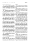
Try just clicking the “Continue” button in Fig 4.1 to use the default evince, which is
usually installed. If it is not, LCMgui will give you a chance to enter another display
command (e.g., gv or okular) in the green field. You can later download and install
28
4.2. TEST RUNS USING LCMGUI
29
Figure 4.1: Here you enter your command for displaying or printing PostScript files.
gv or evince from your Linux distributor’s repository. gv (written by one person
more than 20 years ago) is better than evince for PostScript files; evince is better
for PDF files. It is easy to install gv from the Ubuntu repository. With evince, you
can put an icon on the toolbar for rotating the plot left.
Some Linux distributions (e.g., Ubuntu) have missing fonts or files that cause warnings with evince and the others. Usually, these do not affect the output and can be
ignored. However, LCMgui will ask for a corrected display command. If the display
or printing was successful, you can click “Use Old Command”. You can later suppress
these warnings by using Sec 7.4.6 to change the display command, e.g., to
evince 2>/dev/null
The test runs will automatically output the “One-Page Output” (four pages in this
case). These should approximately agree with PLOTs 1–4 in
$HOME/.lcmodel/doc/figures.pdf.
4.2.2
PostScript Printer
You can instead output to a printer. Most printers can print PostScript files. If your
default printer can, you would probably enter
lpr
in the green entry field in Fig 4.1. For another printer (e.g., called mypr), you would
enter a command like
lpr -Pmypr
30
4.2.3
CHAPTER 4. INSTALLATION AND TEST RUNS
No Printer or Display
If neither printing nor display is possible, then enter the harmless command
touch
in the green field in Fig 4.1. LCMgui outputs the test run results into
$HOME/.lcmodel/test/output/test.ps. You can then transfer this file to a computer that can print or display the file. You could also convert the PostScript files to
PDF files, using Adobe Acrobat Distiller, okular or ps2pdf, present in some Linux
distributions.
If you later find a display or print command that works, you can build this into
LCMgui using Sec 7.4.6.
4.2.4
Further Tests
Without a license and without the test data, LCModel will stop with an error message, but a plot of the absolute value of the spectrum (without a referencing shift
correction) will still be output. Therefore, this plot will indicate whether your data
have been correctly converted and read by LCModel.
You can continue with your first session, or you can exit and start LCMgui again
with the following commands:
cd $HOME/.lcmodel
./lcmgui
You can test the automatic conversion of your data as follows:
• Click on the “Further tests” button when the run with the LCMgui test
data is finished, or click on “Test My Data” when you restart LCMgui
later.
• In Fig 6.3, click on the data type corresponding to your data. (See Sec 3.7.)
• In Fig 6.1, select your data file. (See also Sec 6.2.1.)
• LCMgui should automatically convert your data and plot the absolute
value of the (unreferenced) spectrum in the LCModel One-Page Output.
(Keep in mind that the absolute value of a spectrum has much poorer
resolution than the real part.)
• For CSI data sets: only one voxel near the center will be selected. Section 4.2.5 allows you to display whole slices from 2D & 3D data sets.
4.2.5
More Complete Test of LCMgui with a False License
You can test all facilities of LCMgui by installing a false license.
• First make a false basis file with the commands:
mkdir -p $HOME/.lcmodel/basis-sets
touch $HOME/.lcmodel/basis-sets/dummy.basis
4.3. TEST RUNS WITHOUT LCMGUI
31
• With Linux, simply enter
touch $HOME/.lcmodel/license
With Sun, SGI or DEC/Compaq, install the license (Sec 7.2.5), by entering
any name next to “License OWNER:” and an integer 1–9 digits long next
to “License KEY:”.
• You can then select one of your data files. You can then use the full LCMgui
with the numerous possibilities documented in Chaps. 6 & 7. You can try
setting everything up for possible future routine analyses and archival.
• When you click “Run LCModel” in Fig 6.4, you may (or may not) be asked
to select a Basis Set. Select any file, e.g.,
$HOME/.lcmodel/basis-sets/dummy.basis; LCModel will exit before it
is used.
• LCModel will still only output the absolute value plot with the licensing
message, but the files will now also be archived, as specified in Sec 7.3.3.
You can set up and test the archival system and the rest of the configuration
that you would use with a valid license.
4.2.6
Starting Over
LCMgui remembers what you have done so far. You can make as many test conversions of your data as you wish, but, if for some reason you want to start again
from the very beginning, i.e., from the test run, you can clear LCMgui’s memory by
entering:
rm -fr $HOME/.lcmodel/profiles
You can then start again as though you had just downloaded and unpacked the
whole package by entering:
$HOME/.lcmodel/lcmgui
Then click the “Repeat Test Run” button.
4.3
Test Runs without LCMgui
Until a few years ago, there was no LCMgui. You can still use LCModel directly,
without LCMgui. It is easiest to do the usual installation with the two commands
at the beginning of this chapter. If the test runs are not done (e.g., because X
windows is not running), everything that you need will still be installed (mainly in
$HOME/.lcmodel/bin/).
You can do the test runs without LCMgui with the commands
cd
$HOME/.lcmodel/bin/testrun
32
CHAPTER 4. INSTALLATION AND TEST RUNS
The One-Page Output is then in the PostScript file
$HOME/.lcmodel/test/output/test.ps
On Linux systems, run-time messages about “Skipping namelist · · ·: Seeking namelist
· · ·” are normal and harmless.
Chapter 5 specifies how to prepare and analyze your data either directly with LCModel
or by using the “Other” button (Sec 7.4.4) with LCMgui.
4.4
Benchmark Timings
To compare several computers, you can execute the following command on each:
$HOME/.lcmodel/bin/time-testrun
The test run will be executed and then the time will be output on the screen.
On a Linux platform, no other computationally intensive process should be running,
since the elapsed time is measured. With Unix (Sun, DEC/Compaq or SGI), this
is less critical, since the LCModel CPU time is usually measured. Unix computers
typically take about 150 seconds. Recent Linux PCs typically take about 5 seconds.
Chapter 5
Running LCModel without
LCMgui – Basic Input
Although all users would benefit by becoming familiar with the Control Parameters
in the chapter, LCMgui users with GE, Marconi/Picker, Philips, Siemens, Toshiba
& Varian data can skip this chapter; LCMgui does all this for you. Only LCMgui
users with other data types (using the LCMgui “Other” button).
Instead of using LCMgui, you can run LCModel directly with a command like
$HOME/.lcmodel/bin/lcmodel < my.control
where my.control is a .CONTROL file (Sec 5.3) containing changes to the Control
Parameters.
This chapter specifies the necessary Control Parameters that you may have to set
for the conditions in your laboratory. It also outlines how you would write a simple
Pre-Formatting Program or script to automatically do this and to connect files to
LCModel. The Normal User then only needs to input one name identifying the data.
5.1
Conventions
5.1.1
File extensions
LCModel filetypes are denoted by extensions below. (For clarity, this manual uses
upper case; LCMgui generally uses lower case, except for RAW; you do not have to
follow either of these conventions.)
LCModel needs three input files:
.RAW for the LCModel .RAW file with time-domain data, defined in Sec 5.2. (GE
& Siemens “raw” files will be referred to in lower case.)
.BASIS for a file containing the Basis Set of model metabolite Basis Spectra, defined in Chap 8.
33
34 CHAPTER 5. RUNNING LCMODEL WITHOUT LCMGUI – BASIC INPUT
.CONTROL for the file with the changes to the Control Parameters input to LCModel,
defined in Sec 5.3.
For a given acquisition protocol and field strength, the .BASIS file is generally the
same, whereas the .RAW and .CONTROL files must be prepared for each spectrum.
Some other extensions used in this manual are:
.PS for a PostScript file that you can display or send to your PostScript printer;
.IN for a file with analogs to Control Parameters input to the MakeBasis,
PlotRaw or KECC programs in the LCModel package.
5.1.2
Control Parameter Conventions
When a Control Parameter is defined in this manual, its name (6 or fewer characters) is followed by its Fortran type in parenthesis. Some examples of Fortran type
specifications are:
character*56 means a string of a maximum of 56 characters enclosed in single
quotes, as
NAMREL = ’Cr’
Note that the string ’Cr’ is case sensitive, but the Namelist name
NAMREL is not. Thus you could also use
namrel=’Cr’
but not NAMREL = ’cr’.
integer(20) means an integer array with up to 20 elements, as for KEY in Sec 5.3.
In the .CONTROL file, you could specify the first two elements of the
KEY array as
KEY(1)=12345 KEY(2)=23456
logical can be assigned the value .TRUE. or .FALSE., However, you can also
use T or t instead of .TRUE. and F or f instead of .FALSE.. LCMgui
and this manual use T and F; e.g.,
BRUKER = T
5.2
.RAW File
“RAW” is used to stress that the raw data should never be smoothed or windowed.
Smoothing destroys information and ruins the statistical tests in LCModel.
An example is provided by the .RAW file with the test data in
$HOME/.lcmodel/test/raw/test.RAW. A .RAW file consists of two Namelist headers
preceding the time-domain data itself, as specified in the rest of this section:
5.2. .RAW FILE
5.2.1
35
Namelist SEQPAR
The Namelist SEQPAR is optional, but very useful. If it is included, its data will be
compared with that in Namelist SEQPAR of the .BASIS file to be used. Diagnostics
will then warn of inconsistencies between your in vivo data and your model spectra.
The.RAW File begins with the Namelist SEQPAR:
$SEQPAR
ECHOT = 20.
HZPPPM=84.47
SEQ = ’STEAM’
$END
Namelists are used throughout LCModel. See your Fortran Manual for their many
convenient features, or use the Namelists in your LCModel package as guides; Namelists
are very easy to use. The one critical pitfall: the first column of Namelist input is
always ignored; so each line must start with one space. The start of the Namelist is
specified by a $ (which must be in column 2) followed by the Namelist name (e.g.,
$SEQPAR above). The end is specified by $END.
Most convenient is that the Namelist can be very long, but only the variables explicitly
input in the Namelist are changed; the rest keep their original (default) values. Most
Control Variables have default values, and these are specified in this manual. If you
agree with the default of a Control Parameter, then you do not have to input anything
for it. (Exceptionally, none of the Control Variables in Namelist SEQPAR has a default
value.)
The above Control Parameters are:
ECHOT (real) (“echo time”) the echo time (in ms) used for this data.
HZPPPM (real) (“Hz per ppm”) the field strength, in terms of the proton resonance
frequency in MHz, i.e., HZPPPM = 42.58B0 , with B0 in Tesla. You should
input it with an accuracy of at least four significant figures.
SEQ (character*5) must be either PRESS or STEAM, according to the localization method used for this data.
5.2.2
Namelist NMID
The second Namelist in the .RAW file is NMID, and it is always required. An example
is:
$NMID
ID=’pat 777 77’
FMTDAT=’(2E15.6)’
VOLUME=18.0,
TRAMP=89.6,
$END
The above Control Parameters are:
36 CHAPTER 5. RUNNING LCMODEL WITHOUT LCMGUI – BASIC INPUT
ID (character*20) a string that you can use to identify the data. It appears in the so-called Detailed Output and in the plot of the data with the
program PlotRaw. It is useful for documentation, but it is optional; if you
leave it out of the Namelist input, then a blank ID is output.
FMTDAT (character*80) the Fortran format specification for your raw timedomain data, which must immediately follow Namelist NMID. (See also
Sec 5.2.3 below.) This has no default; it must be input.
VOLUME (real) the voxel size (always in the same units, e.g., mL).
Default: VOLUME = 1.0
TRAMP (real) The data are multiplied by the factor TRAMP/VOLUME to scale the
data consistently with the Basis Set, as discussed in Sec 10.1.1. VOLUME
and TRAMP do not affect the concentration ratios; they only need to be
input for absolute concentrations. Default: TRAMP = 1.0.
BRUKER (logical) (“Bruker data”) Bruker, Philips & Toshiba data must have
BRUKER = T, which causes all 4 programs in the LCModel package to complex conjugate the data, which is necessary with these data types. (This
Control Parameter was named before I had contact with Philips or Toshiba
data.)
Default: BRUKER = F
SEQACQ (logical) (“sequential acquisition”) This is for Bruker users only. You
do not need to input this in the normal case of simultaneous acquisition,
where the real and imaginary parts of the complex pair of time-domain
data are acquired simultaneously. If you do not input it, then it will be left
at its default value of SEQACQ = F. Only for Bruker sequential acquisition
mode (default on some Bruker systems prior to the AVANCE series), where
the imaginary part of the complex pair is acquired one sample time after
the real part, must you input SEQACQ = T; in this case, you input the
uncorrected data (as the usual complex pairs), and all 4 programs in the
LCModel package automatically correct the data for you.
So, the only necessary input in this Namelist required from everyone is FMTDAT, if
you are only interested in concentration ratios.
For absolute concentrations, LCModel needs a TRAMP that scales the in vivo data
consistently with the Basis Spectra. VOLUME then accounts for the voxel size. Chapter
10 specifies this in detail. In addition, absolute concentrations are more sensitive than
concentration ratios to the corrections for relaxation (Sec 11.2) and partial-volume
effects (which are all independent of LCModel).
5.2.3
Time-Domain Data
These must start on the line immediately after the $END of Namelist NMID. These
data points must be in order of increasing time, with each point a complex pair (real,
imaginary, real, imaginary, . . . ).
5.3. .CONTROL FILE
5.2.3.1
37
CSI data sets
The time-domain data for one voxel must be immediately concatenated to the preceding time data, with no blank positions between (therefore, a FMTDAT with only
one complex pair per line is safest, e.g., ’(2E15.6)’). There are also no Namelists
SEQPAR or NMID for voxels after the first, only the time data.
This is already the structure of the the time-domain data in Bruker, Philips, Siemens,
Toshiba & Varian files in Sec 3.7, which are automatically handled by LCMgui.
5.3
.CONTROL File
An example from the test runs is the file test.control. The .CONTROL file consists
solely of the the Namelist LCMODL. A simple example is:
$LCMODL
OWNER=’Biomedizinische NMR Forschungs GmbH’
KEY=123456789
TITLE=’pat 777 77 (41Y, M) 18.0ml, gm, PMP’
FILBAS=’/home/lcm/basis-sets/te20 2c.basis’
FILRAW=’pat 777 77.raw’
FILPS=’pat 777 77.ps’
$END
The above Control Parameters are:
OWNER (character*120) the name of the license holder. (With Linux, this is
not used, but the Linux license file must be in $HOME/.lcmodel/license.)
This string is given to you with your license. You must input it exactly,
i.e., with the same capitalization and spacing, all on one line.
KEY (integer(20)) your license key. (With Linux, this is not used, but the
Linux license file must be in $HOME/.lcmodel/license.) This is given to
you with your license. Together with OWNER, it enables you to run LCModel
on the licensed Unix workstation.
TITLE (character*244) the title that you want to appear at the top of the
One-Page Output (and elsewhere).
FILBAS (character*255) the pathname of the .BASIS file to be input.
Note: On most platforms, you cannot use symbols like ∼ or $HOME to
denote your home directory with any Control Parameters.
FILRAW (character*255) the pathname of the .RAW file to be input.
FILPS (character*255) the pathname of the .PS file that will contain the
PostScript One-Page Output.
You will have to add more changes to your .CONTROL file. These are specified in
this chapter. However, these changes are usually always the same; the only Control
Parameters in the .CONTROL file that are normally changed with every data set are
38 CHAPTER 5. RUNNING LCMODEL WITHOUT LCMGUI – BASIC INPUT
TITLE, FILRAW, and FILPS. You should be able to write a simple Pre-Formatting
Program so that the Normal User only has to input one name, e.g., pat 777 77. The
Pre-Formatting Program then
• finds the corresponding raw time-domain data and formats it as the .RAW
file;
• makes the .CONTROL file by extracting TITLE from a header in your original
data file and by inserting pat 777 77 into FILRAW and FILPS;
• runs LCModel and prints or displays the One-Page Output in the .PS file.
In the following, I specify the additional (generally data-set-independent) changes
that your Pre-Formatting Program adds to the .CONTROL file to change the default
Control Parameters to those appropriate for your instrument and protocol. Note that
the ordering in a Namelist is not important, except that a Control Parameter input
several times will take on the value closest to the end of the Namelist. It is therefore
best to add changes to the bottom of the list (just above $END). The table Input
Changes in the One-Page Output prints your .CONTROL file from the bottom up, so
that the most recent changes (at the bottom of the file) are at the top of the table.
5.3.1
Instrument and Acquisition
HZPPPM (real) (“Hz per ppm”) the field strength, in terms of the proton resonance
frequency in MHz, i.e., HZPPPM = 42.58B0 , with B0 in Tesla. You should
input it with an accuracy of at least four significant figures.
Default: HZPPPM = 84.47 (1.984 T; so, you will almost certainly have to
input your own value.)
NUNFIL (integer) (“N unfilled”) the number of complex pairs of data points in
one scan, without zero-filling. Default: NUNFIL = 2048
DELTAT (real) (“δt”) the time (in s) between two consecutive real points (or two
consecutive imaginary points). This is just the sample time or “dwell time”
or the reciprocal of the “bandwidth.” Default: DELTAT = 0.0005
The acquisition time for one scan, DELTAT*NUNFIL, should be long enough so that
the in vivo time-domain data decay into the noise. For brain spectra at 1.5 T, this
is typically 0.8 s or 1.0 s. At higher fields it is usually shorter.
5.3.2
Multi-Voxel Data Sets
One voxel’s data is immediately concatenated to the preceding one’s. We use the
DICOM standard that the voxels in the file start at the top left and are ordered as
in three nested loops, with the columns in the inner loop, the rows in the middle
loop, and the slices in the outer loop; i.e., the voxels are row-after-row, then sliceafter-slice. Thus, the second voxel’s data in the file is said to come from Column 2
of Row 1 of Slice 1 (assuming that there is more than one column). Scanner displays
are not always consistent with this (Sec 11.4.3.2).
5.3. .CONTROL FILE
39
You specify the CSI data set dimensions of the .RAW file with the following Control
Parameters:
NDCOLS (integer) (“Number of data columns”) The number of columns in the
CSI data set.
Default: NDCOLS = 1
NDROWS (integer) (“Number of data rows”) The number of rows in the CSI data
set.
Default: NDROWS = 1
NDSLIC (integer) (“Number of data slices”) The number of slices in the CSI data
set.
Default: NDSLIC = 1
You specify the range (rectangular subset) of voxels to be analyzed by LCModel with:
ICOLST & ICOLEN (integer). Voxels in columns ICOLST through ICOLEN will be
analyzed.
Default: ICOLST = ICOLEN = 1
IROWST & IROWEN (integer). Voxels in rows IROWST through IROWEN will be analyzed.
Default: IROWST = IROWEN = 1
ISLICE (integer). Voxels in slice ISLICE will be analyzed.
Default: ISLICE = 1
There will now be a set of output files for each voxel, and these are uniquely identified
as follows: the Slice# (only for 3D sets) and Row# & Col# are inserted at the
beginning of each TITLE (as in PLOT 15 in $HOME/.lcmodel/doc/figures.pdf).
The output filenames are extended as in the following example: if you input FILPS =
’filename.ps’, then the Slice#1, Row#2, Col#3 file will be filename sl1 2-3.ps.
Section 11.4.3 lists other cases and also specifies how to change the format of these
identifiers.
Section 11.4 specifies how to combine .PS files into a single file, and how skip over a
voxel in the rare case that it causes an abort, breaking off the multi-voxel analysis.
5.3.3
Analysis Window
You select the Analysis Window (the window of frequency-domain data that will be
analyzed) as follows:
PPMEND (real) (“ppm end”) the lower limit of the ppm-range; i.e., the right edge of
the Analysis Window (with the usual convention of the ppm-axis decreasing
toward the right).
Defaults: See Sec 3.4.1.
PPMST (real) (“ppm start”) the upper limit of the ppm-range; i.e., the left edge
of the Analysis Window.
Default: PPMST = 4.0
40 CHAPTER 5. RUNNING LCMODEL WITHOUT LCMGUI – BASIC INPUT
These two Control Parameters are the most important ones for salvaging problem
spectra. They are probably the only two that the Normal User will also want to
occasionally change. See Sec 3.4 for guidelines.
5.3.4
Eddy-Current Correction
Philips users can skip Sec 5.3.4; you should have Philips do the eddy-current correction (ECC) as specified in Sec 3.7.6.
With single-voxel brain data, eddy-current correction [10] is recommended. This
requires also a reference fid from the same voxel with the same sequence, except with
no water suppression. With a CSI data set, all of the voxels in the unsuppressed
reference data set must be the same as those in the suppressed data set. However,
ECC is often ineffective with CSI data and is seldom done.
These reference data are automatically included with the water-suppressed data in
a single-voxel GE Probe raw P-file or Marconi/Picker file, and the two required
LCModel .RAW files (see Sec 9.6) can be made. In other cases, you have to organize
this yourself: You put the unsuppressed reference data in a separate file (FILH2O).
You then add DOECC & FILH2O, as specified in Sec 9.6 to your .CONTROL file.
In addition to improving the Baseline and lineshapes, ECC usually greatly reduces
the zero-order phase correction. Section 9.7.1 shows how you can experimentally
investigate whether this correction is small. If it is, then this prior knowledge can
speed up and improve the LCModel analysis, especially of poor quality spectra. With
single-voxel data, add the following Control Parameter to your .CONTROL file to impose this prior information:
SDDEGZ = 6.
(The Index at the end of this manual tells you where to find the discussion of other
Control Parameters, such as SDDEGZ.)
With CSI data, ECC may be less effective and the phases highly variable. Do not
input SDDEGZ; let the Bayesian learning in LCModel set SDDEGZ.
For Bruker users only: In ParaVision,choose the option to have ECC done. Do not do ECC
again in LCModel. Without LCMgui, you first correct these for Bruker’s digital filter using
Bruker’s convdta. Do not input SDDEGZ, since the zero-order phase correction is often not
small.
In rare cases, particularly if the water suppression is weak and the unsuppressed water
reference not very good, you may see that ECC obviously amplifies the noise in the
high-ppm part of the spectrum. If this amplified noise extends into the Analysis
Window, then you should switch off ECC by removing DOECC and SDDEGZ from the
.CONTROL file, for this spectrum only.
5.3. .CONTROL FILE
5.3.5
41
First-Order Phase Correction
The first-order phase correction (φ1 ) is often small, and prior knowledge of this can be
used to speed up and improve analyses. At least two well-separated landmark peaks
are needed to determine the zero-order and first-order phase corrections. Therefore
prior knowledge of phases is very important with spectra lacking two strong landmarks, as in PLOT 6 in $HOME/.lcmodel/doc/figures.pdf (although this case also
worked without specifying SDDEGZ or SDDEGP).
As specified in Sec 9.7, the Control Parameter SDDEGP tells LCModel the standard
deviation of the expectation value, DEGPPM, of the first-order phase correction. The
following seem to work well for single-voxel data:
• GE Probe data:
SDDEGP = 1.
• Marconi/Picker data with STEAM and current PRESS sequences:
SDDEGP = 2.,
DEGPPM = 2.5
• Marconi/Picker data with very old PRESS sequences:
SDDEGP = 2.,
DEGPPM = 28.
If you are not sure whether your PRESS sequence is “older” or “newer,”
then try both 28 and 2.5 for DEGPPM; they are very different, and the wrong
one should give very poor phasing. If you are in doubt, send me two or
three “dump” files with high-quality PRESS spectra.
Siemens data often have a big φ1 . However, this is usually quite consistent, i.e.,
also with a small SDDEGP, as with the Marconi/Picker values, which were calculated
from their precisely known timing. Section 9.7.1 shows how you can experimentally
estimate DEGPPM and SDDEGP.
5.3.6
PostScript Output
Section 9.9.3 gives many possibilities to tailor the format of the One-Page Output
to your wishes, even for preparing slides or figures for publication. In any case, you
should input the following Control Parameter:
PGNORM (character*2) (“page norm”) ’US’ sets the page dimensions of the OnePage Output to 8.5 × 11.0 inches;
’A4’ or ’EU’ sets the dimensions to 21.0 × 29.7 cm.
The default is PGNORM = ’ ’ and makes a compromise to fit in both page
formats.
Usually there is not enough room for the complete tables to the right of the plots in
the “One-Page Output”. Then, by default, a second page with the complete tables
(and no plot) is produced. Therefore, you should use a duplex printer, if possible, so
that both pages are on one sheet.
IPAGE2 (integer)
IPAGE2 = 0 to suppress printing the second page (e.g., if you do not have
a duplex printer), thereby losing information;
IPAGE2 = 1 (the default) to output a second page (PLOT 2 in
42 CHAPTER 5. RUNNING LCMODEL WITHOUT LCMGUI – BASIC INPUT
$HOME/.lcmodel/doc/figures.pdf) with the complete tables, if there is
not enough room on the first page;
IPAGE2 = 2 to always output a second page with the tables.
5.3.7
Archiving the Results
The .PS and .TABLE files contain the essential graphic and numeric information from
the analysis. The .CSV file contains the concentrations and can be imported to
spreadsheet programs. With LCMgui, you can select any of these to be output using
Fig 7.3.
5.3.7.1
.TABLE File
The .TABLE file contains all the information in the tables of the One-Page Output
as a self-documented text (ASCII) file. You can archive these files (particularly if
you have assigned them unique pathnames with FILTAB) into a database (e.g., for
computing means or other statistics over a group of spectra). For this, you must
input the following:
FILTAB (character*255) (“table file”) the pathname of the .TABLE file to be
output. (e.g., ’/home/user1/.lcmodel/saved/pat 777 77/table’).
LTABLE (integer)
LTABLE = 0 (the default) will suppress creation of this file;
LTABLE = 7 will make this file.
5.3.7.2
.CSV Spreadsheet File
The .CSV file for spreadsheets is convenient for multi-voxel analyses (Sec 11.4.4). (For
single-voxel analyses, it consists of only two very wide rows of concentration data.)
FILCSV (character*255) the name of the .CSV file to be output (e.g.,
’/home/user1/.lcmodel/saved/pat 777 77/spreadsheet.csv’). A file
with the extension .csv (but not a file simply with the name csv) is
automatically imported as a “comma-separated-value” file by spreadsheet
programs.
LCSV (integer)
LCSV = 0 (the default) will suppress creation of this file;
LCSV = 11 will make this file.
5.3.7.3
.PS PostScript File
The .PS file is output automatically. It contains all the information in the One-Page
Output, including the plotted curves. You could archive this in the same directory
as the .TABLE file. You can then view it with a PostScript viewer (Sec 4.2.1). You
can also archive it on paper using a (duplex) PostScript printer.
5.3. .CONTROL FILE
5.3.7.4
43
.COORD Coordinate File
If you want to make your own plots, the .COORD file contains the coordinates of all
curves on the One-Page Output (in an easy-to-read and self-explanatory text file):
FILCOO (character*255) (“coordinate file”) the name of the .COORD file to be
output (e.g., ’/home/user1/.lcmodel/saved/pat 777 77/coord’).
LCOORD (integer)
LCOORD = 0 (the default) will suppress creation of this file;
LCOORD = 9 will make this file.
5.3.8
Phantoms
Tests with in vitro data from model solutions are unrealistic and not always useful.
The accuracy and spectral resolution in the Basis Set must be higher than that in
the data, and this is often not the case here. Broadening the in vitro test data also
smooths them, and this falsifies the statistical tests [11] in LCModel. Even without
smoothing or broadening, the systematic errors in such data often exceed the normal
scatter due to the noise, and this falsifies the model itself.
Your phantom data at room temperature will be inconsistent with simulated basis
sets using data from 37◦ C.
If you are analyzing in vitro data, then use
VITRO (logical) .TRUE. if the spectrum is an in vitro spectrum; this will override
some statistical tests that could otherwise be falsified with such data.
Default: VITRO = F
If necessary, increase AQ, the acquisition time for one scan, so that the time data
have decayed into the noise.
In addition, your phantom spectrum must be dominated by at least one of the following: NAA, Cr or Cho. Otherwise, you will have to set additional parameters
as illustrated in Sec 11.6. So, it is much simpler if your phantoms always contain
significant amounts of at least one of the above 3 landmark metabolites.
Even simpler is when you are doing standard calibrations either of the scanner
(Sec 10.1.2) or of the Basis Spectra (Sec 8.7.1). Then, VITRO=T (and several other
Control Parameters) are automatically set.
Chapter 6
Elementary Guide to LCMgui
This chapter gives the basic steps for the Normal User in using LCMgui, with references to Chap 7 for details. Chapter 4 gives the simple steps for downloading and
installing LCMgui. Chapter 7 is a detailed reference, allowing you to make full use
of the flexibility of LCMgui and to optimally configure LCMgui for the Normal User.
LCMgui remembers many of the settings from the previous run. If an expert user has
already made runs from your account, then you may not have to change any settings,
and the following three simple steps may be sufficient:
• Start LCMgui (Sec 6.1).
• Select the file containing the data to be analyzed (Fig 6.1 in Sec 6.2.1).
• Click on “Run LCModel” (Fig 6.4 in Sec 6.4).
Parts in this fine print are seldom necessary reading, but they can help you make better use of
LCMgui. If you are one of the first to run LCMgui from this account, then you should check the
points in fine print.
6.1
Starting LCMgui
LCMgui is installed under one or more usernames. You must log on using one of
these usernames. Log in normally, as the user, not as root. You can then always
start LCMgui with:
$HOME/.lcmodel/lcmgui
LCMgui may have been installed so that you can also start it with simply:
lcmgui
6.2
Selecting the Data to be Analyzed
See Sec 3.7 for a list of the types of data files automatically handled by LCMgui and
for important guidelines.
44
6.2. SELECTING THE DATA TO BE ANALYZED
45
Figure 6.1: The File Selector, shown here for GE LX files
6.2.1
File Selector Window
When LCMgui is started, the first window that appears is usually the File Selector.
An example with GE Signa LX data is shown in Fig 6.1. With data from other
manufacturers, the title, “Select your GE Signa LX . . .” will be different. LCMgui
remembers the directory where the data file was in the last run, and the File Selector
starts there.
If you have several User Profiles, then the window in Fig 7.12 will appear first. Normally, you
immediately click on “Use Selected Profile” to continue using your present User Profile.
If the last LCMgui session did not use Bruker, GE, Marconi/Picker, Philips, Siemens, Toshiba or
Varian data, then the window in Fig 6.3 will appear first. You normally then click the “Other”
button in Fig 6.3, as you did in the previous session.
If no license has been installed, a window will first appear offering you the chance to test the
conversion of your data (as in Sec 4.2.4).
You first navigate through the directory tree. When you click on a directory, its
files are listed in the right pane (the stage shown in Fig 6.1). You then click on the
filename that you want to use and click the yellow “OK” button at the right (or
simply double-click on the filename).
Only filenames that match the filter shown at the top of the pane of filenames (p*.7, P*.7 or
P*.7.??) in Fig 6.1) are displayed. If your filename differs from this standard (e.g., if you analyzed
GE Signa 5.x data last time and LX data this time), then it will not be listed. You can change
46
CHAPTER 6. ELEMENTARY GUIDE TO LCMGUI
Figure 6.2: You selected a file of the wrong type in the File Selector
the filter by clicking on the field (p*.7 P*.7 P*.7.??), pressing the “backspace” or “delete” key,
entering your new filter (e.g., *), and pressing the “Enter” key.
If you want to also see files or directories that start with a dot (e.g., .lcmodel/), then click on the
“Show Hidden Files” button on the right to make it yellow.
If the filenames or directories in Fig 6.1 are so long that they are cut off, then the width of the panes
can be adjusted by holding the left mouse button down on the small square at the top on the pane
boundary (between “Directories:” and “Files:”) and dragging the pane boundary. (You can also
simply use the scroll bar that appears at the bottom of the pane when names are too long.)
6.2.1.1
Selecting the wrong file type
LCMgui remembers what type of data was analyzed from this account and User Profile the last time,
and it expects the same type this time. You therefore get a window like Fig 6.2 if in the File Selector
you:
• Select a file of another type (e.g., a Siemens “raw” file after GE Signa LX last time). If you
have data of different types (e.g., GE and Siemens), then you should use a different User
Profile (Sec 7.3.7) for each. This way, the default settings for each data type are preserved
and kept separate.
• Select a completely irrelevant file (e.g., p-wrong-type.7 in Fig 6.1 to produce Fig 6.2).
If you selected the wrong User Profile at the start of session, then you can click the “Abort LCMgui”
button, and then restart and select the correct User Profile.
Otherwise, click the yellow “Retry” button in Fig 6.2. A window like Fig 6.3 appears. Here you click
on the appropriate type of data. The File Selector then returns, giving you another chance to select
your data file.
6.3
Control Parameters Window
After you click the “OK” button in the File Selector, the second of the two most
important windows, the “Control Parameters” window (Fig 6.4), appears. LCMgui
remembers most of the settings from the previous session. Thus, Normal Users
often can simply click the yellow “Run LCModel” button at the bottom to start the
LCModel analysis. (Yellow is generally used to show you the usual path to take.)
6.3. CONTROL PARAMETERS WINDOW
47
Figure 6.3: Note that GE Signa 5.x and LX (or higher) have distinct buttons.
However, you should check the following in your “Control Parameters” window, at
least during your first runs. (Most of the fields have balloon help messages that pop
up if the cursor remains over a field for 3 seconds.)
6.3.1
Analyzing spectrum from:
In the second row in Fig 6.4, the entries next to “Analyzing spectrum from:”
define the Analysis Window, the ppm-range over which the spectrum will be analyzed
(Sec 3.4). You can change this range by clicking on the green up or down arrow next
to the value. (Green usually indicates fields that you can click on or edit to make
changes.)
You may want to change these values to cut off artifacts (Sec 3.6.1).
6.3.2
BASIS file:
In the third row in Fig 6.4, the entry next to BASIS file: shows the pathname of the .BASIS file
containing the model spectra that will be used to analyze your data. If the .BASIS files are installed
as specified in Sec 7.2.4, then LCMgui should automatically select the proper one, if it exists. Also
LCModel normally produces diagnostics if the .BASIS file does not match your data.
For the first runs, you should nevertheless check whether the entry is correct. (STEAM or PRESS
and TE should be visible in the filename.) If it is wrong, you cannot edit the white field (only green
48
CHAPTER 6. ELEMENTARY GUIDE TO LCMGUI
Figure 6.4: The Control Parameters Window
fields). Instead you click on the green “Change BASIS” button, and you get a File Selector for your
.BASIS file, which you select just as in Sec 6.2.1.
6.3.3
Do eddy-current correction
Philips users can skip Sec 6.3.3; you should have Philips do the eddy-current correction (ECC) as
specified in Sec 3.7.6.
Users with Toshiba, Marconi/Picker data or GE Probe P-files can skip Sec 6.3.3 since eddy-current
correction (ECC) is done automatically. Other users only have to set this as default the first time
for future analyses. In the fourth row in Fig 6.4, a mouse-click switches the button for ECC between
active (blue) and inactive (no ECC). (Blue usually indicates a button that is switched on.)
ECC is recommended for single-voxel data (but not for CSI, where it is usually ineffective). You then
must also have acquired an unsuppressed water reference spectrum from the same voxel immediately
before or after acquiring your water-suppressed spectrum. With a CSI data set, all of the voxels in
the unsuppressed reference data set must be the same as those in the suppressed data set. If you
have this reference data file, be sure to make the ECC button blue.
In rare cases, particularly if the water suppression is weak and the unsuppressed water reference
not very good, you may see that ECC obviously amplifies the noise in the high-ppm part of the
spectrum. If this amplified noise extends into the Analysis Window, you should switch off ECC for
this spectrum only.
6.3.4
Do water-scaling
Water-Scaling uses the unsuppressed water reference signal (as used above for ECC) to estimate
absolute concentrations. Section 10.2.2 discusses the significant uncertainties in the corrections
needed for this. Chapter 10 also discusses an alternative for Siemens Vision and 1.5T GE data,
using Calibration Phantoms.
You activate Water-Scaling simply by making the “Do water-scaling” button blue. However, Sec 10.2.2
specifies important additional Control Parameters that you may have to change from their default
values. Sections 7.3.4 & 7.3.5 specify how to change Control Parameters and save these changes for
future use.
6.3. CONTROL PARAMETERS WINDOW
49
Concentration ratios are not affected by Water-Scaling and are less sensitive to relaxation and partialvolume effects.
6.3.5
Only for Multi-Voxel data files:
If you only have single-voxel data, then you can skip this section and this part of the
“Control Parameters” window.
The balloon that pops up over this part gives step-by-step instructions on previewing
a whole slice and then selecting a rectangular subset to be analyzed. It also gives
troubleshooting hints.
Some headers do not have complete information on the total numbers of slices, rows
& columns in the data file, even though LCMgui still correctly converts the file. So,
you should first check and (if necessary) correct these values (usually signaled by a
-1).
The “Preview Data” button at the bottom of the “Control Parameters” window is
especially important with CSI data sets. Details and troubleshooting hints are given
in Sec 7.4.1.
6.3.5.1
Multi-Voxel output
You get one PostScript output file for each voxel. If your default display/print command is a display command, then you will get a series of displays that each have to
be closed before you view the next. It is usually more convenient to suppress the
display/print command by deleting it using Sec 7.4.6. You can then use Sec 11.4.5
to combine all the files into one for convenient viewing.
6.3.6
The Rest of the Control Parameters Window
The rest are briefly listed here, with references to more detailed descriptions. They make LCMgui
very flexible.
TITLE: This field at the top of Fig 6.4 will also appear at the top of the One-Page Output. You
can edit this field, e.g., to insert comments on location or pathology.
Save File Types See Sec 6.5.
Advanced Settings Clicking this button produces a menu (Fig 7.6) offering several new windows.
In this menu, the “View/Edit Control Parameters” window allows you to view, change,
delete or add Control Parameters. For example, if the ECC button in Sec 6.3.3 was off
and you turned it on (blue), then you should check the Control Parameter SDDEGZ, as
specified in Sec 7.3.4.
Preview Data This allows you to first view your data (in the time- and/or frequency-domain, on
your screen or printer), e.g., to make sure that you have the correct data and that it is
worth analyzing. (Sec 7.4.1)
6.3.7
Reload Data
The TITLE: line or “Preview Data” may cause you to wonder whether you selected
the correct data file. You can further check this by moving the mouse (without
50
CHAPTER 6. ELEMENTARY GUIDE TO LCMGUI
Figure 6.5: The instructions-part of the File Selector for the unsuppressed water
reference.
clicking it) to the “Reload Data” button at the bottom. A balloon message will
appear showing the filename that you selected. If this file is incorrect, you can click
on the “Reload Data” button; the File Selector window will appear, and you can
start over selecting a new data file; i.e., you start again at Sec 6.2.1.
6.4
Run LCModel
Once you are satisfied with the settings in the “Control Parameters” window, you
click the yellow “Run LCModel” button at the bottom. Normally, the analysis is
immediately started (as a background process), and a new window appears offering
you the chance to start another analysis by selecting a new data file and proceeding
again from Sec 6.2.1. (You can start a new analysis before previous analyses have
finished; as each analysis finishes, its results are automatically output.) However,
four windows may appear before the analysis can start:
Select unsuppressed water reference file If the “Do eddy-current correction”
button is active (blue), the File Selector window appears (unless you have
Marconi/Picker files or GE Probe P-files, which already contain the water
reference). It is exactly as in Fig 6.1, except for the window of instructions
at the upper left (Fig 6.5). As you can see from Fig 6.5, the filename
of your currently selected water-suppressed data is shown, and you must
select the corresponding unsuppressed data file.
With Philips, Siemens, Toshiba and GE spectrum G-files, if the voxel
locations of the two files do not coincide, then a window appears with an
error message and with options for continuing or starting over. LCMgui
cannot always extract accurate voxel positions from Siemens syngo files,
and this warning is sometimes a false alarm; if you are sure that the voxels
match, then you can simply click the button “Do Wrong Water” to continue
with the analysis.
Missing data If LCMgui is not able to extract all necessary information from the
data files, new windows will prompt you for these values.
6.5. WHERE IS THE OUTPUT?
51
Overwrite archive files? LCMgui automatically archives the output in an Archive
Directory that is usually unique for each data file. However, if you want
to analyze a data file for a second time, a window will appear warning
you that the old output is about to be overwritten. You are given the
opportunity of aborting, changing the output directory or overwriting it.
Save changes? If you have changed any Control Parameters (e.g., activated the
“Do water-scaling” button), a window offering you the chance to save these
changes for possible future use as defaults appears. This can be very useful
in saving you from having to remember and enter these changes in the
future. This is described in Sec 7.3.5.
6.5
Where is the Output?
Normally LCMgui automatically outputs the One-Page Output with a print or display command
that was specified during installation in Sec 4.2.2. If you cannot find your output, Sec 7.4.6 specifies
how you can check and correct this print or display command.
There are several other useful files that can be output and archived by LCModel. Clicking on “Save
File types” in Fig 6.4 produces a menu where you can select which types of output files will be
archived. In addition to the .PS file (with the One-Page Output), the .TABLE file (with tables
summarizing the results) should be selected.
The green field following “Save File types to directory:” (which you can edit) shows the directory
where they will be archived. See Sec 7.3.3, which also specifies how you can change the structure of
this Archive Directory tree.
By default, the filename is simply the type of output, e.g., ps is the .PS file and table is the .TABLE
file. By default, for multi-voxel (CSI) data sets, they are made unique as in the following example:
The Slice#2, Row#3, Column#4 .PS filename is sl2 3-4.ps.
The “input changes” table in your One-Page Output also has information on file locations:
SAVDIR (“Save-Directory”) shows the directory where the output was archived.
SRCRAW (“Source of RAW file”) gives the full pathname of the data file that you chose with the File
Selector.
SRCH2O (“Source of H2O file”) gives the full pathname of the unsuppressed water reference file (if you
chose one).
6.6
Interactive Processing with LCMgui
Normally, you use LCMgui to start a series of analyses, without waiting for one to end before starting
the next. However, your analyses may go fast enough that you would want to run “interactively”,
viewing the LCModel results of one analysis on your terminal before starting the next.
Section 7.4.2 specifies how to do this. If this has been implemented, then you should wait for the
results to be displayed on your screen. To continue with LCMgui, you must then exit the display
program yourself.
6.7
Getting out of LCMgui
LCMgui usually has an “Exit LCMgui” or an “Abort LCMgui” button. When you
click this, you are usually given the choice of four buttons (Fig 6.6):
52
CHAPTER 6. ELEMENTARY GUIDE TO LCMGUI
Figure 6.6: Here you decide how to save the settings from this session.
Exit & Save : This is the normal exit. LCMgui exits and saves the changes that
you have made to LCMgui settings (such as the locations of your
Basis and data files). When the next LCMgui session is started,
these will then be offered as defaults.
Do Not exit : to cancel the exit and continue with LCMgui;
Exit & Forget : LCModel exits, but does not save any settings that you made
during this session. When the next LCMgui session is started, you
will be offered the same defaults that you were offered at the start of
this session. This can be helpful if you have made some big mistakes
during this session, or if you used some unusual settings that you do
not want to have saved as defaults for the future.
New Profile : allows you to save your settings to a new User Profile, using the
window in Fig 7.12. You should use different profiles for different
types of data (e.g., GE & Philips or 1.5T & 3T).
If the normal LCMgui exit buttons are not available, then enter Control-C or
Control-Z in the Linux/Unix window from which you started LCMgui.
Chapter 7
LCMgui Reference Manual
This chapter will allow you to fully exploit the flexibility of LCMgui. It will also allow
you to optimally install & configure LCMgui for less experienced Normal Users.
You must be familiar with Chap 6.
7.1
LCMgui Structure
The main steps executed by LCMgui are:
(1) File Selector. You select the file containing your (binary scanner) data
to be analyzed with the window in Fig 6.1.
(2) Data Conversion. A program is executed to produce the LCModel .RAW
file and any available Control Parameters (e.g., NUNFIL, DELTAT) from
the file selected in Step (1). You can specify this program to be the
standard LCMgui program for the standard Bruker, GE, Marconi/Picker,
Philips, Siemens, Toshiba or Varian files (Sec 3.7). However, there is also
an “Other” button to use a script supplied by you for another type of file.
(3) Preprocessor. Even if you specify one of the standard programs for
Step (2), you can still supply your own script in this step to modify the
.RAW file or Control Parameters from Step (2). (The original default, when
LCMgui is installed, is to use no Preprocessor.)
(4) Control Parameters Window. This window (Fig 7.2) allows you to
make many checks of the data and modifications of the Control Parameters
and the LCMgui configuration before starting LCModel. You can also
configure LCMgui so that the Normal User usually only has to click “Run
LCModel” at the bottom of the window, without much knowledge of the
rest.
(5) Run LCModel. When you click the “Run LCModel” button, LCMgui
makes many checks and then starts an Execution Script in background.
The default script starts LCModel and archives the results. However, this
script is available to you as a template, and you can modify it for your own
53
54
CHAPTER 7. LCMGUI REFERENCE MANUAL
purposes.
The possibility of supplying your own scripts in Steps (2), (3) & (5) makes LCMgui
very flexible. At the same time, LCMgui remembers most settings from the previous
run; so, if you make the first analyses after installation, Normal Users with limited
knowledge can often analyze their data with your configuration. You can even prevent Normal Users from permanently changing your most important settings (using
Sec 7.5.1.2).
7.1.1
Limitations
Unlike LCModel (which was written by one person and is quite self-sufficient), LCMgui
combines free software from several sources and depends on your particular window
manager and system. With Linux, some window managers (especially old ones) may
on rare occasions require that you manually move and resize some windows. Sometimes, you get a tiny window (smaller than an icon), which you have to find (usually
toward the upper left), click on and then resize; it is best to then exit and start
LCMgui again.
Most displays have sufficient resolution for LCMgui. The display must have at least
1024 × 768 pixels (better 1600 × 1200 or 1280 × 1024); 800 × 600 pixels are not
enough. If the LCMgui windows are only slightly too large, then you can try reducing
the font size (Sec 7.5.1.4).
7.2
Installing LCMgui
As specified in Chap 4, downloading from the WWW site on Page 2 and installing
(and uninstalling) are very simple. Do not work as root; for example, this could set
file access privileges so that LCModel updates by the user do not work properly. The
entire package goes into $HOME/.lcmodel/ of the user’s directory.
However, you can avoid continually entering the dot and everywhere use lcmodel
instead of .lcmodel by entering:
cd
ln -s .lcmodel lcmodel
7.2.1
Multi-User Installations
One license allows an unlimited number of users to have LCMgui and LCModel
installations. An unlimited number of users can simultaneously run LCMgui and
LCModel on the licensed computer. You could install into a new account and have
all users use this installation. This would make installing upgrades simpler. However,
it is better if each user has their own installation (as with a browser), so that their
settings and archive of results are not overwritten by others. This also allows them
to decided if or when to upgrade. (Upgrades are free.)
7.2. INSTALLING LCMGUI
7.2.2
55
Starting LCMgui
You start LCMgui with the command
$HOME/.lcmodel/lcmgui
If you set your PATH environment variable to include $HOME/.lcmodel, then you
should be able to start LCMgui simply with:
lcmgui
7.2.3
First Test Runs
LCMgui uses most of the settings from the previous run as defaults for the current
run. So, your first runs are most important, since the Normal User can then later
successfully use LCMgui often simply by selecting the data file and clicking “Run
LCModel”.
The most important initial settings at this stage are:
Output: You set the print (or display) command in the initial test run (Sec 4.2.2),
and all future results will be automatically output in this way.
Section 7.4.2 specifies how you can both print and simultaneously display
the results on your monitor.
You can also completely avoid printing, by displaying only and using the
archived .PS and .TABLE files for later reference. (Most display programs
allow you to print anyway.)
Data File Type: In the second test (Sec 4.2.4) during installation, you select the
data type in Fig 6.3 and test the automatic conversion and input of data
to LCModel.
If you do not have the automatically convertible file types specified in
Sec 3.7, then Sec 7.4.4 specifies how you use your own data conversion
script with the “Other” button in Fig 6.3.
7.2.4
Install Model Spectra
You need a Basis Set of model metabolite spectra compatible with your data, as
specified in Sec 8.1. We have a large collection of basis sets (especially for PRESS)
freely available for use with LCModel. Be sure to contact me first before acquiring
your own using Chap 8.
To install the basis sets, first unzip them (e.g., with gunzip) and then be sure to mv
them to the directory $HOME/.lcmodel/basis-sets/.
7.2.4.1
Multiple Field Strengths
You can skip this unless you have data acquired at more than one field strength.
LCMgui does not use field strength to select default Basis Sets. Here is a detailed
56
CHAPTER 7. LCMGUI REFERENCE MANUAL
Figure 7.1: The Install License Window (with Sun, SGI or DEC/Compaq)
example of how you can separate field strengths:
Suppose that you have 1.5T & 3T data.
• mv your 1.5T Basis Sets into the directory $HOME/.lcmodel/basis-sets/
• For your 3T Basis Sets:
mkdir $HOME/.lcmodel/basis-sets/3t
and mv the 3T .BASIS files into this directory.
• The first time that you analyze 3T data, click the “Change BASIS” button in
Fig 7.2 and then select the appropriate 3T basis file from the 3t/ directory.
• When you exit from this first 3T session, click “New Profile” in Fig 6.6, enter
“3T” in Fig 7.11, and then click “Save”.
• At the start of future LCMgui sessions, Fig 7.12 allows you to select “1” (for your
1.5T User Profile) or “3T” (for your 3T User Profile). This way, you keep your
1.5T and 3T Basis Sets, archives of results, default settings, etc., separate.
• When you exit from LCMgui sessions after the first 3T session, you can exit
normally by simply clicking ”Exit & Save” in Fig 6.6.
7.2.5
7.2.5.1
Install License
Linux
You receive your license file attached to an email. You install it simply with the command:
mv license $HOME/.lcmodel/
If your email comes through some other system, it might rename the file license.dat or
license.bin. Be sure that the file is correctly renamed back to license. be sure to transfer
license to your Linux computer using “binary” mode (not “ascii” and not “text” mode).
7.2.5.2
Sun, SGI or DEC/Compaq
After you have completed the test runs, a window appears with an “Install License” button.
Clicking this produces the window in Fig 7.1. You enter the information that you received
with your license. After clicking “OK” and accepting the License Agreement from the website
7.2. INSTALLING LCMGUI
57
on page 2, the File Selector (Sec 6.2.1) appears, and you are ready to start the first analysis
of your data; see Sec 7.3.
be sure to exit normally from LCMgui, with the “Exit & Save” button in Fig 6.6, so that
your license information is saved.
7.2.5.3
GE SAGE/LCModel interface
With Linux, set the following in your .sagerc file:
setenv LCM OWNER ‘‘dummy’’
setenv LCM RUNKEY 123
(They are not used by the Linux version.) With Sun, SGI or DEC/Compaq, replace dummy
above with the OWNER string provided with your license, and replace 123 above with the value
for KEY provided.
When you run the SAGE/LCModel interface, the window titled “LCModel Analysis” appears.
Be sure to make the following changes in every session:
SDDEGZ: 999.0 (only for CSI)
SDDEGZ: 3.0 (only for single-voxel data)
SDDEGP: 1.0
Start PPM: 4.0
End PPM: 0.2
Section 3.4.1 discusses cases where you might want to use other values for End PPM: (PPMEND).
There is reportedly a configuration file, where you can set these values once, for all future
analyses.
Missing from the Concentration Table in the output are the important Concentration Sums
NAA+NAAG and probably Cr+PCr and the sum of all choline-containing compounds GPC,
PCh & Cho (Sec 2.1.1). You will have to compute these sums yourself. It is important to
use only these sums (e.g., NAA+NAAG) and not the much less accurate individual estimates
(e.g., NAA and NAAG). Similarly, if PCr is estimated, compute the concentration ratios to
Cr+PCr instead of the ratio to only Cr.
7.2.6
Installing Updates & Upgrades
(“Updates” and “upgrades” are used here interchangably.) Updates to any parts of the package will normally be incorporated into a complete new updated LCModel/LCMgui package
(not patches).
If you also wish to save your old LCModel package (e.g., for perfect compatibility in longitudinal studies) before updating, you can enter:
cp -a $HOME/.lcmodel $HOME/.lcmodel-old
Then in the future (after updating) you can switch to the old version with:
mv $HOME/.lcmodel $HOME/.lcmodel-new
mv $HOME/.lcmodel-old $HOME/.lcmodel
(You can also use symbolic links.)
Do not delete your old $HOME/.lcmodel; instead install your update “on top of” your old
installation. You install an update simply by downloading from
http://lcmodel.ca/lcm-test.shtml and installing with the two commands:
tar xf lcm-???.tar
./install-lcmodel
where ??? is linux, sun, sgi or dec.
58
CHAPTER 7. LCMGUI REFERENCE MANUAL
The test run will automatically be done, but you can then continue as before, since only
files that have changed in the update will be modified. Your license and other configuration
settings will not be changed. Any files that you have added or archived in the $HOME/.lcmodel
directory tree will also be preserved.
The only exception is that you should not manually modify any of the files originally delivered
with LCMgui, since these are overwritten by an update. However, this is normally never done
and is never recommended in this manual.
be sure to exit normally from LCMgui, with the “Exit & Save” button in Fig 6.6, so that all
of your update information is saved.
7.3
Basic Settings and Usage
The first runs are the most important, since LCMgui uses your previous settings as defaults
for the future. This section shows the most important settings, which can often allow you
and inexperienced Normal Users to make future analyses with only a few mouse clicks.
For the first run, you should follow Chap 6, including all the fine print. Particularly important
are your settings in the “Control Parameters” window (Fig 7.2) for the Analysis Window
(Sec 6.3.1) and deciding whether to use eddy-current correction (Sec 6.3.3) and/or WaterScaling (Sec 6.3.4).
See Sec 3.7 for important guidelines and for a list of the types of data files automatically
handled by LCMgui. Also note the following:
7.3.1
Vendor-Specific Guidelines
Bruker, Marconi, Toshiba, Varian: To avoid writing outside of $HOME/.lcmodel/ during testing, the initial default Archive Directory is $HOME/.lcmodel/saved/. Section 7.3.3.3 specifies how to archive in a more convenient place (near your original
data).
Bruker: With single voxel data, the files acqp and method must be in the same directory
as your data file fid.
If the file method is missing, you have a very old ParaVision version. The instructions at the beginning of the (text) file $HOME/.lcmodel/bruker/bin2raw show
you how to proceed.
GE: Section 7.4.5.1 describes Preprocessors that are important in the following special
cases:
• when you are not using automated Probe and your data require large phase
corrections;
• when you want to select frames to salvage a spectrum damaged by patient
motion during part of the acquisition;
• when you are not using the standard 5000 Hz bandwidth with 3T data.
Marconi/Picker: Only if you are using PRESS: You will probably have to select the Preprocessor new-press (Sec 7.4.5). Prior phase information is very accurate, and
LCMgui uses this. However, older and newer PRESS sequences have very different
values. For backwards compatibility, the older values are used by default. Try a
few analyses with and without the Preprocessor new-press. The wrong choice
should yield very poor phasing. If in doubt, send me two or three “dump” files
with high-quality spectra.
7.3. BASIC SETTINGS AND USAGE
59
Philips: Be sure to use Sec 3.7.6.
Siemens: Since a wide variety of Siemens files are accepted, you may select totally irrelevant
files (e.g., with 2N bytes), and they may be accepted. This can be checked with
“Preview Data” (Sec 7.4.1), but it is also usually apparent from errors in the
TITLE: line in Fig 7.2. You can then click “Reload Data” in Fig 7.2.
Further important settings are in the following sections:
60
CHAPTER 7. LCMGUI REFERENCE MANUAL
Figure 7.2: The Control Parameters Window
7.3.2
.BASIS file
Your .BASIS files should go into the directory $HOME/.lcmodel/basis-sets/. Then, LCMgui
normally automatically selects the correct Basis Set, based on the information in the scanner
data files. In some cases, information is missing (e.g., TE in older GE spectrum G-files),
and you should check the entry next to “BASIS file:” in the “Control Parameters” window
(Fig 7.2) and click the “Change BASIS” button if necessary. If you are using only .BASIS
files supplied by me, then you can skip the rest of Sec 7.3.2.
LCMgui attempts to automatically select the correct .BASIS file from the default Basis directory (the
Basis directory from the last session). It first attempts to extract TE and the localization sequence
(STEAM/PRESS) from your data headers. It then attempts to find the corresponding .BASIS file,
whose filename must satisfy the following rules:
TE: The filename must contain the string teNNN (including underscores at each end), where
NNN is the integer value of TE in ms. An example is:
gamma press te8 300mhz 070.basis
steam/press: The appropriate string must be in the filename.
File Extension: This must be .basis, .BASIS or .Basis.
7.3.3
Archiving the LCModel Results
You can specify which type of output will be archived by LCMgui and where it will
be archived. It is obviously best to organize this data base as soon as possible.
7.3.3.1
Which File Types will be Archived?
Clicking on the “Save File types” in the “Control Parameters” window (Fig 7.2)
produces the menu in Fig 7.3. You click on a filetype to make its button blue to
have LCMgui archive it in this (and each future) session. By default, the .TABLE file
(a compact tabular summary of the results useful for later statistical and data base
7.3. BASIC SETTINGS AND USAGE
61
Figure 7.3: You get this menu when you click the “Save File Types” button
in Fig 7.2.
analyses) and the .PS file (with the One-Page Output) are archived. See the Index
at the end of this manual for the other filetypes in Fig 7.3.
7.3.3.2
In which Directory will they be Archived?
The directory where these files will be saved is shown in the green field. The following
are the default structures:
Bruker, Marconi/Picker, Toshiba, Varian: $HOME/.lcmodel/saved/
(see Sec 7.3.3.3 for a good alternative)
GE raw P-files: the standard SAGE data-base hierarchy:
$HOME/.lcmodel/saved/Site/PatientID/Study/Series/
GE spectrum G-files: As with P-files, except that your Site is replaced with
from-G-file, since LCMgui cannot recover the Site from G-files.
Philips: $HOME/.lcmodel/saved/examination name/patient name/scan date/.
An alternative script, where scan id is also available is available from me.
Siemens: $HOME/.lcmodel/saved/<PatientName> <the part of the DataSetId
following ‘‘/’’>
Here, Site/PatientID/Study/Series, examination name/patient name/scan date,
PatientName & DataSetId are all taken from header information, which can vary
with each spectrum. Therefore, the directories are often unique for each spectrum.
If you are satisfied with these defaults, then you can skip the rest of Sec 7.3.3.
You can edit the green field next to “to directory:”, but this new directory will only
be used during this one analysis.
62
CHAPTER 7. LCMGUI REFERENCE MANUAL
Figure 7.4: The window for permanently reconfiguring the structure of (Bruker)
Archive Directories.
7.3.3.3
Reconfiguring the Archive Directory Tree
You can permanently change the Archive Directory tree structure by clicking on the
“Reconfigure” button in Fig 7.2, which produces a window like Fig 7.4 for Bruker,
Marconi, Toshiba & Varian data. For these four data types, a good alternative to
their original default Archive Directory ($HOME/.lcmodel/saved/) is in the same
directory as the original scanner data. (This is not the default for safety reasons only
— all original default output of LCModel/LCMgui is confined to $HOME/.lcmodel/.)
The instructions in Fig 7.4 are quite detailed, but the following step-by-step example,
may be useful:
(1) Click the green “Append” button next to “Original Data Directory”.
(2) Enter pdata/lcmodel in the green field next to “Enter a fixed element”,
and then click the “Append Entry” button to the right. This is the stage
shown in Fig 7.4.
(3) If you are satisfied with the structure shown in the field next to “Constructed Save Directory:”, then click the “Set Configuration” button.
For example, the LCModel output .PS file will be
/tmp/lcm/binary-data/bruker/r0107/pdata/lcmodel/ps
For Marconi, Toshiba & Varian data, you might enter lcmodel rather than pdata/lcmodel
in Step (2).
7.3. BASIC SETTINGS AND USAGE
63
Note the following:
• You can experiment, watching your progress in the field next to “Constructed Save Directory”, and undoing mistakes by clicking the “Start
Over” button.
• You can cancel everything that you have done in the present “Configure
Save Directory” window by clicking the “Cancel” button.
• Your changes only take effect when you click the “Set Configuration”
button.
• Even after “Setting Configuration”, you can always click on “Change Configuration” to further modify or correct the configuration.
• You can restore the original LCMgui default Save Directory configuration
by clicking on “Change Configuration” and then on “Restore Default”.
• No matter how badly you have messed things up, you can always start
over completely, as specified in Sec 7.5.1.1.
• You can protect your configuration from being accidentally permanently
changed, as specified in Sec 7.5.1.2.
7.3.3.4
Reconfiguring for File Extensions
Normally, the .PS file is a file called ps in the Archive Directory. The following
Siemens example using Fig 7.5 shows how to archive them as extensions to filenames.
(1) Click the green “Append” button next to “Default Save Directory”.
(2) Click the green “Append” button next to “PatientName:”
(3) Enter (underscore) in the green field next to “Enter a fixed element”, and
then click the “Append Entry” button to the right.
(4) Click the green “Append” button next to “Tail of Data SetId:”.
(5) In the green field next to “Enter a fixed element”, delete the underscore
and enter .* (period then asterisk), and then click the “Append Entry”
button to the right. This is the stage shown in Fig 7.5.
(6) If you are satisfied with the structure shown in the field next to “Constructed Save Directory:”, then click the “Set Configuration” button.
This special dot-star (.*) combination at the end of the Archive Directory causes
LCMgui to make a file extension. In this example, the .PS file will be
/SP/sp/.lcmodel/saved/vol 2401 148.ps. Without the dot-star at the end, the
file would be /SP/sp/.lcmodel/saved/vol 2401 148/ps; i.e., a slash would replace
the dot, and the extension would become a file.
7.3.4
View/Edit Control Parameters
LCMgui gives you the full capability of comfortably setting all Control Parameters
in this manual. You can also save these settings for optional use as defaults later.
64
CHAPTER 7. LCMGUI REFERENCE MANUAL
Figure 7.5: The window for permanently reconfiguring the structure of (Siemens)
Archive Directories.
Figure 7.6: You get this menu when you click the “Advanced Settings” button in
Fig 7.2.
7.3. BASIC SETTINGS AND USAGE
65
Figure 7.7: You can view, edit, delete or add all Control Parameters here.
You do this by clicking on the “Advanced Settings” button in the “Control Parameters” window (Fig 7.2). This produces the menu in Fig 7.6. You then click on
“View/Edit Control Parameters” in this menu to obtain the window in Fig 7.7. This
shows the Control Parameters that will be input to LCModel. You can edit or delete
these or add new ones. For example, Fig 7.7 shows where I have added SDDEGZ &
HZPPPM at the bottom. (Case is not important for the names of Control Parameters;
only strings within single quotes are case-sensitive.)
With GE Probe raw P-files and Marconi/Picker data, eddy-current correction (ECC)
is automatically done by LCMgui. Otherwise, during your first runs, you should
decide whether you can do ECC. Sections 9.6 & 9.7 discuss ECC and the settings
of SDDEGZ & SDDEGP. (However, LCMgui automatically sets the Control Parameter
FILH2O mentioned in Sec 5.3.4 for you.)
During one of your first runs you should also enter PGNORM in this window. (See the
Index at the end of this manual for terms like PGNORM.) If you print, then you should
use a duplex printer; otherwise you will also want to enter IPAGE2=0.
7.3.5
Saving Your Control Parameters
If you have made any changes to Control Parameters, the window in Fig 7.8 will
appear after you click “Run LCModel”. Only the modified Control Parameters are
shown, but you are offered the chance of saving all the Control Parameters for optional
use in the future. You can click the “Save Changes” button. This produces the
window in Fig 7.9.
In Fig 7.9, you enter a name for the file that will store your Control Parameters. This
is called a Control-Defaults File. In Fig 7.9, I have entered the name g-files-ecc.
66
CHAPTER 7. LCMGUI REFERENCE MANUAL
Figure 7.8: You can save all the Control Parameters, including your modifications,
for optional use as starting defaults in the future.
Figure 7.9: Here you enter a name for the file which will store your Control Parameters
for optional future use.
You are free to choose any descriptive filename. However, if it is identical with one
of the filenames listed at the bottom (e.g., bm10), then your file will overwrite the old
file.
If you click “Use Next Time” in Fig 7.9, then this set of Control Parameters will be
used as defaults for future sessions. LCMgui will still reset obviously variable Control
Parameters, such as TITLE, FILRAW, etc.
In addition, LCMgui may reset some Control Parameters (e.g., SDDEGZ & SDDEGP) to their commonly
used values. The only way to avoid having to manually set them back to their desired values every
time is to use a Preprocessor (Sec 7.4.5).
If you click “Save”, then your Control Parameters will simply be archived for optional
use later. They will not be used as defaults for the next session. The old Control-
7.3. BASIC SETTINGS AND USAGE
67
Figure 7.10: Here you select the Control-Defaults file to be used now and in the
future.
Defaults File used at the start of this session will again be used.
7.3.6
Changing your Default Control Parameters
How do you know what file Control-Defaults file is currently being used? You again
click on “Advanced Settings” in Fig 7.2. The Control-Defaults file currently being
used is in parentheses next to “Change Control-Defaults file”. In Fig 7.6, there
is nothing between the parentheses, indicating that no file is being used (i.e., the
conversion program called by LCMgui solely determines the starting values of the
Control Parameters).
You can change the Control-Defaults file currently being used as follows:
• Click on the “Advanced Settings” button in Fig 7.2 to produce the menu
in Fig 7.6.
• Click on “Change Control-Defaults File” to produce the window in Fig 7.10.
(If there is no Control-Defaults file in your directory, then you will be told
this and given the chance to continue.)
• The currently used file is shown in the green field, under “Selected File”.
68
CHAPTER 7. LCMGUI REFERENCE MANUAL
Figure 7.11: At the end of a session, you can select a new User Profile where all of
your settings from the session will be saved.
(The original default is no Control-Defaults File; the green field would then
be blank.)
• As explained in Fig 7.10, you can select a new Control-Defaults File by
clicking on its name, which then appears in the green field.
• Click “Use Selected File”, and LCMgui immediately repeats the conversion
of your data and applies these new Control Defaults. This newly selected
Control-Defaults File will also be used in the future (until you change it
again).
Note that the Control-Defaults File only provides you with starting defaults. You
can then modify these values as you wish in the “Control Parameters” window.
7.3.7
User Profiles
There are two sets of default settings, one for LCModel and one for LCMgui. The
Control-Defaults file (Sec 7.3.5) contains default Control Parameters for LCModel.
The gui-defaults file contains default settings for LCMgui, including the ControlDefaults file path, directories for archiving results and finding Basis Sets, etc. Both
of these sets of defaults are saved in your User Profile.
If you have different types of data that require different LCMgui settings (e.g., different Archive Directories), then you should have a User Profile for each. This would
always be the case with data from different scanner types (e.g., GE and Siemens).
Different users sharing the same account could also have different User Profiles.
You create a new User Profile by clicking on “New Profile” in Fig 6.6, which appears
as you exit LCMgui. The window in Fig 7.11 appears, and you enter the name of the
User Profile. In Fig 7.11, I have entered toshiba. You may choose any descriptive
7.4. FURTHER USEFUL SETTINGS
69
Figure 7.12: At the start of a session, you select the User Profile to be used.
directory name. However, if it is identical with one of the names listed at the bottom
(e.g., 1), then your default files will overwrite the old files.
If you enter toshiba as your User Profile, then your gui-defaults will be in
$HOME/.lcmodel/profiles/toshiba/gui-defaults and all Control-Defaults files that you
save from this User Profile will be in the directory
$HOME/.lcmodel/profiles/toshiba/control-defaults/. You can look at their contents
with the usual Unix commands, but do not edit them. You can delete obsolete ControlDefaults files, e.g., with
rm $HOME/.lcmodel/profiles/toshiba/control-defaults/bm10
Your initial User Profile is 1. You can rename this (or any of your others) by a command like
mv
$HOME/.lcmodel/profiles/1 $HOME/.lcmodel/profiles/siemens
When you start LCMgui, Fig 7.12 allows you to select any one of your User Profiles
for that session (if you have more than one User Profile from previous sessions).
7.4
7.4.1
Further Useful Settings
Previewing Data
Clicking “Preview Data” at the bottom of the “Control Parameters” window (Fig 7.2)
produces the window in Fig 7.13. As explained there, by editing the green field next
to “Print the plot with command:” to your command for displaying or printing
PostScript files and then clicking on “Run Preview”, you can display or print plots of
the data before starting LCModel. This can be useful in checking whether you have
selected the correct data file and whether the data are worth analyzing.
You can activate both the “Display or print...” & “Second display...” buttons to
both print and display.
70
CHAPTER 7. LCMGUI REFERENCE MANUAL
Figure 7.13: Here you can set and execute your commands for printing and/or plotting previews of your data.
If possible, orientation and magnification should be supplied in the display command,
since trying to change these in the display program can sometimes crash the display
program and LCMgui, particularly if you are working over a slow network. For
example, you might use gv -orientation=seascape.
With multi-voxel data sets, you can select a complete 2D slice with Fig 7.2, or a
rectangular subset. If your selection contains more than one voxel, then Fig 7.13
will indicate this voxel range, and will only offer a plot of the absolute value spectra
(in a 2D array, as in PLOT 14 in $HOME/.lcmodel/doc/figures.pdf). This display
(following the DICOM standard) may not always be consistent with the scanner’s
display (Sec 11.4.3.2).
If you want to save the plots, they are in a file with a name of the form
$HOME/.lcmodel/temp/12d-21h-51m-09s-996pid/plotraw.PS
where the numbers will be different, as explained in Sec 7.5.2.2. Copy this to a safe place, since the
above directory will be deleted with the next analysis.
If no plot is produced, check your plot and display command. If a diagnostic message, ‘‘Aborting
due to error ... Check User’s Manual’’, appears in your Unix window, then check Sec 8.5.3.
Check that your selected data file is correct. Finally, you could start LCModel, which has extensive
diagnostics.
7.4. FURTHER USEFUL SETTINGS
71
Figure 7.14: Here you can select the Execution Script that will be started by LCMgui.
7.4.2
Interactive Processing
Normally you use LCMgui to start LCModel analyses in background, without waiting
for one to end before starting the next. However, your analyses may go so quickly that
you would want to run “interactively”, viewing the LCModel results of one analysis
on your terminal before starting the next.
If you can display PostScript files on your terminal (as discussed in Sec 7.4.1), then
Sec 7.4.6 shows how to change the command for printing your LCModel output to a
display command. The one limitation of this interactive mode is that you should wait
for one analysis to end before starting the next (to avoid multiple displays popping
up).
7.4.3
Execution Scripts
As outlined in Sec 7.1, the final step of LCMgui is to start an Execution Script in background. By default, this script is $HOME/.lcmodel/execution-scripts/standard.
You should not edit this script. However, you can copy it and use it as a template
for your own customized scripts. It contains suggestions on possible changes.
You must also put any Execution Scripts that you make into the directory
$HOME/.lcmodel/execution-scripts/.
The currently active Execution Script is shown in parentheses next to “Change Execution Script” in Fig 7.6. If you click “Change Execution Script”, the window in
Fig 7.14 shows you how to select another Execution Script for now (and for the
future).
7.4.3.1
Batch Processing
Normally you use LCMgui to start LCModel analyses in background, without waiting for one to end before starting the next. However, if your workstation is slower
72
CHAPTER 7. LCMGUI REFERENCE MANUAL
processing analyses than you are in starting them, you may want to avoid overloading
it with many simultaneous jobs.
The Execution Script nice helps by reducing the priorities of the LCModel analyses,
but a much more effective way is to use the Execution Script make-batch, as follows:
• Select the Execution Script make-batch in Fig 7.14.
• Prepare and start your analyses as usual, clicking “Run LCModel”, one
after another.
• Exit LCMgui and enter
$HOME/.lcmodel/bin/run-batch
Only then will the analyses be started, one after another, one at a time.
• The start and finish times, as well as any run-time error messages appear
on your screen. All run-time messages (including harmless ones) go into
$HOME/.lcmodel/temp/batch-messages.
7.4.4
Processing Non-Standard Data Files
LCMgui’s first computation step [Step (2) in Sec 7.1] is to produce LCModel input
files from the data file that you selected in Step (1) in Sec 7.1. LCMgui does this by
executing
$HOME/.lcmodel/???/bin2raw, where ??? = bruker, ge5, gelx, marconi,
philips, siemens, toshiba, varian or other, depending on the type of data file
that you specified in the menu in Fig 6.3.
Actually, LCMgui first attempts to execute $HOME/.lcmodel/???/my-bin2raw. If
my-bin2raw does not exist, then it executes bin2raw. This gives you the opportunity of copying bin2raw to my-bin2raw and modifying my-bin2raw to your special
purposes. Your my-bin2raw will be preserved, since only bin2raw is overwritten
during LCMgui updates.
Normally, you would produce other/my-bin2raw, and use the “Other” button in
Fig 6.3 for your special-purpose processing. $HOME/.lcmodel/other/bin2raw provided with LCMgui does no data conversion; it simply assumes that your selected
file has already been converted to LCModel .RAW format (Sec 5.2). However, the
comments in this script also specify what you must do to prepare your particular
type of data files.
After you make your special other/my-bin2raw, then, in your next LCMgui session,
select your non-standard file with the File Selector. Your previous LCMgui session
probably did not use the file type “Other”, and you will then get the error window
in Fig 6.2. Click “Retry” and then select “Other” in the window in Fig 6.3 to use
your customized script in other/my-bin2raw.
The scripts bruker/bin2raw and philips/bin2raw provide further examples and
specifications on preparing your own my-bin2raw script or executable program. Particularly philips/bin2raw contains arbitrary assumptions (e.g., on filenames) which
you can easily modify to your needs.
7.4. FURTHER USEFUL SETTINGS
73
Figure 7.15: Here you can view and/or change the Preprocessor that will be used by
LCMgui.
Even after you make other/my-bin2raw to handle your file types, the instructions in the File Selector
will still (incorrectly) tell you that you must select an LCModel .RAW file.
7.4.5
Optional Preprocessor
This is Step (3) in Sec 7.1. It gives you the opportunity of modifying the Control
Parameters or the .RAW file computed from your standard data conversion in Step
(2).
Only files in the directory $HOME/.lcmodel/???/preprocessors/ will be available as
Preprocessors in Figure 7.15. Here, ??? = bruker, ge5, gelx, marconi, philips,
siemens, toshiba, varian, or other, depending on which type of data you selected
in Fig 6.3.
Your own Preprocessor scripts must also be in this directory.
$HOME/.lcmodel/doc/preprocessors/README.txt explains how to make your own
Preprocessor.
You can check the Preprocessor currently being used by clicking “Advanced Settings”
in Fig 7.2. The current Preprocessor is in parentheses next to “Change Preprocessor”.
In Fig 7.6, there is no Preprocessor is being used.
You can then change the Preprocessor as follows:
74
CHAPTER 7. LCMGUI REFERENCE MANUAL
• Click on “Change Preprocessor” to produce the window in Fig 7.15. (If
there is no Preprocessor script in the directory, then you will be told this
and given the chance to continue.)
• The currently used script is shown in the green field, under “Selected File”.
(The original default is no Preprocessor step; the green field would then
be blank.)
• If you want to use another Preprocessor now (and in the future), then click
on its name, and its name will also appear in the green field as the “Selected
File”. Then click “Use Selected File” and the selected Preprocessor would
be executed immediately (and in the future, until you change it).
7.4.5.1
GE Preprocessors
The following Preprocessors are available for GE data:
change-phase-priors : GE automated Probe spectra usually need only very small
phase corrections, and this prior information is used by default. However,
this can cause huge phasing errors, if you have non-standard data requiring large phase corrections. If analyses of non-standard data show poor
phasing, then you should first edit the file
$HOME/.lcmodel/???/preprocessors/change-phase-priors as explained
in the file (where ??? = ge5 or gelx). Then select this Preprocessor in
Fig 7.15.
select-frames : can salvage a spectrum that has been damaged by patient motion. You can select a subset of frames that excludes the period where
there was motion (or other damage). Full instructions are in the comments in $HOME/.lcmodel/gelx/preprocessors/select-frames. Note
that LCMgui must not be running in background; i.e., it must not have
been started with a “&” at the end of your command. select-frames is
not available for 5.x data or for multi-channel data.
set-3t-bandwidth : LCMgui assumes that the bandwidth of 3T data is 5000Hz. If
this is not the case with your 3T data, then edit the file
$HOME/.lcmodel/gelx/preprocessors/set-3t-bandwidth as instructed
in the comments there. Then select this Preprocessor in Fig 7.15.
use-unsuppressed : (Cannot be used with multi-channel (phased array) data.) It
will cause the unsuppressed water reference frames to be analyzed instead
of the usual water-suppressed frames. You acquire many water reference
frames and only a small number of water-suppressed frames (there still
must be at least one, although it is not used). This is used instead of
Water-Scaling to get a direct and unified analysis of a single spectrum
including the water signal, for example for bone marrow. (Sec 9.3).
7.4.6
Changing the License & the Print Command
These settings were made during installation. You can change them as follows:
7.5. FINE POINTS
75
• In the main “Control Parameters” window, click on “Advanced Settings”
to get the menu in Fig 7.6.
• Click on “Change LCMgui Settings”. This produces a window with entries
containing the current OWNER and KEY license settings (as in Fig 7.1) and the
print (or display) command that LCMgui is currently using for outputting
the LCModel PostScript file. (With Linux, there are no OWNER and KEY
entries.)
• Edit any of these entries that you want to change and click on “OK”, or
click “Cancel Changes” to cancel your changes and leave everything as it
was.
One common change is to delete the entire print command, leaving the entry blank
(which is not accepted during installation). This suppresses printing and display, but
not the archiving of the plots in the .PS files. This can be useful if you are processing
many spectra (e.g., a multi-voxel data set) and want to view the results later from the
archive. You can later collect all of the .PS files into one file for convenient viewing
using Sec 11.4.5.
7.5
7.5.1
Fine Points
gui-defaults Resource File
LCMgui stores all of your default settings for future sessions in
$HOME/.lcmodel/profiles/???/gui-defaults, where ??? is your currently selected User Profile (1 by default). Each line consists of a one-word index (e.g.,
i displayCommand), whitespace, a value (e.g., gv --orientation=seascape), and
nothing else on the line. In exceptional cases listed below, you may wish to edit this
file. You should only edit the value and only as specified below.
7.5.1.1
Starting Over
If you hopelessly corrupt gui-defaults, you can always recover by deleting
gui-defaults. When you start LCMgui the next time, it will be as with a new
installation. You first click “Repeat Test Run”, then install the license (unnecessary
with Linux), and then proceed with data analysis. All of your previous defaults (and
mistakes) will be forgotten.
7.5.1.2
Protecting your Settings
You can make the initial LCMgui runs and optimize the default settings for Normal
Users. During any future LCMgui session, the user can modify any of your settings.
Normally, LCMgui will store these new settings in gui-defaults for use as defaults
for the next session. However, you can prevent LCMgui from storing changes to
critical settings by changing the value of i preserveConfiguration in gui-defaults
76
CHAPTER 7. LCMGUI REFERENCE MANUAL
from “0” to “1”:
i preserveConfiguration 1
Some of the critical defaults that are protected by the above setting are:
• The structure of the Archive Directory for LCModel results and which
types of output files will be saved there;
• The default .BASIS file;
• The print and display commands;
• The pathnames of the files with the default Control Parameters, the Preprocessor and the Execution Script;
• The license data.
In this way users have full freedom to change everything for their present session,
but they and others are protected from the most critical of their changes in future
sessions.
7.5.1.3
Data Filename Filters
The File Selector window in Fig 6.1 will only display filenames that match the filter, which is specified by the values i fileType*, where * = Bruker, Ge5, GeLx,
Marconi, Other, Philips, Siemens, Toshiba or Varian. You can temporarily
enter a new filter in the entry below “Files:” in Fig 6.1. However, you can permanently change this in gui-defaults. For example, you can specialize
i fileTypeSiemens *
to
i fileTypeSiemens *.rda
7.5.1.4
Window & Font Size
You may find the LCMgui windows too big. The best way to reduce them is to increase the resolution of your display. Otherwise, you can slightly reduce the windows
by reducing 10 in
i fontPoints 10
Missing fonts in your Linux/Unix distribution may cause the characters to be poorly
displayed. Changing i fontPoints 10 above may help, although the best collection
of fonts is often 10-point.
7.5.1.5
Help Balloon Delay
Particularly in the “Control Parameters” window, balloons with help messages pop
up after the cursor has been over a field for
i balloonWait 3000
ms. A smaller value may be useful to beginners, but irritating to experienced users.
7.5. FINE POINTS
7.5.1.6
77
Colors
The five colors specified in gui-defaults all have (self-explanatory) indices beginning
with i color. For example,
i colorFollowMe yellow
specifies that the normal path to take is denoted by yellow buttons. You can change
these values to symbolic names (e.g., red) or by hexadecimal numbers preceded by
a # (e.g., #ff0000) with the RGB value. Your X-Windows system must be able to
assign the color. (This manual will then no longer be correct in its color references
to buttons and fields.)
7.5.2
7.5.2.1
Cleaning up the File System
Obsolete User-Defined Files
You can produce and save arbitrarily many files with Control-Defaults, Preprocessors
and Execution-Scripts. They are saved in
$HOME/.lcmodel/profiles/***/control-defaults/
$HOME/.lcmodel/execution-scripts
$HOME/.lcmodel/???/preprocessors
where *** is your User Profile and ??? = bruker, ge5, gelx, other, marconi,
philips, siemens, toshiba or varian. You can always examine these in their
directories and delete the obsolete ones.
You can also (be careful with rm -fr) delete a whole User Profile with a command
like
rm -fr $HOME/.lcmodel/profiles/my-profile
7.5.2.2
Temporary Files
These are automatically purged, and you normally do not have to bother with them.
Each LCModel analysis typically requires only about 200 kB of temporary disk storage (more with CSI data).
They are all in $HOME/.lcmodel/temp/. Each time LCMgui prepares data for an
LCModel analysis, a unique temporary directory is created, e.g.,
$HOME/.lcmodel/temp/12d-21h-51m-09s-996pid
The numbers are, respectively, the day of the month, hour, minute, second and
process ID.
When the LCModel analysis is finished, the directory is marked for deletion, and is
deleted when the next LCModel analysis is prepared. So, directories only remain for
LCModel analyses not completed (including aborts from LCMgui). By default, these
remaining directories are deleted if they are more than 86400.0 s (1 day) old. You
can modify this value in the following line in gui-defaults:
i deleteAfterSeconds 86400.0
Chapter 8
Making the Basis Set
It is only necessary to read this chapter if you must collect your own Basis Set of in
vitro model metabolite spectra. Your in vivo data must be compatible with the Basis
Set, as specified in Sec 8.1. If you have been supplied with a Basis Set, and your data
will always satisfy the compatibility requirements in Sec 8.1, then you do not need
to read the rest of this chapter. Before acquiring model spectra, check with
me to see if a basis set compatible with your data is already available. We
have a large collection freely available for use with LCModel.
Your in vivo spectra are analyzed as a linear combination of these Basis Spectra.
Your efforts in getting a good Basis Set are well invested, since this will be the basis
of the analyses of probably thousands of spectra. This is not a nice little project for
a student. It requires great care and expertise.
An alternative is simulating the basis spectra [12]–[15].
8.1
Compatibility Requirements
The following conditions in your in vivo data must be the same as those in the Basis
Set:
•
•
•
•
B0 field strength (only to within a few %)
Localization sequence (e.g., STEAM or PRESS)
T E (to within a few ms)
T M (with STEAM) (to within about 5–10 ms)
The following do not have to match: T R, the spectral bandwidth or the acquisition
time per scan.
78
8.2. MODEL METABOLITE SOLUTIONS
8.2
8.2.1
79
Model Metabolite Solutions
Choice of Model Metabolites
Table 8.1 shows most of the metabolites that have been used with LCModel. At low
fields (up to 2.35 T) and moderate T E (up to 80 ms), all metabolites in the upper
part of the table are recommended. Note that you do not buy Glyc (or any other
metabolite with only a singlet in the Analysis Window); you simulate Glyc simply
by inputting into LCModel (Sec 11.7):
NSIMUL = 14
Under the following other conditions:
long TE: Asp, GABA, Glc, GPC (indistinguishable from PCh) & NAAG (a shifted
NAA can simulate NAAG) are unnecessary.
high fields: Considerably more metabolites can be quantified above 4.7 T, especially
at short T E [16].
The metabolites in the bottom part of Table 8.1 occur in pathologies and some may
be necessary for your studies.
It is better to measure too many than too few metabolites. You should include all
metabolites that you will conceivably ever want to use. With Control Parameters in
Sec 9.8.1, you can easily exclude irrelevant Basis Spectra from an analysis, and for
consistency it is best to acquire all Basis Spectra in one session, rather than adding
new ones later.
Whenever possible, use salts rather than acids, in the interests of better pH control.
The order numbers in the table were kindly supplied by users who obtained spectra
with no apparent contamination. They are the latest that I have, but most are
outdated. Reports of contaminated metabolites are listed below. For example, it
seems important to use L-Lactic acid and L-Alanine; D/L mixtures of Lac from
several sources were contaminated.
The Basis Spectra must have both higher accuracy and resolution than the in vivo
spectra. Higher concentrations are useful in achieving this. The recommended concentrations are in column 3. NAAG and GPC are expensive, but do not go below
their minimum concentrations in Table 8.1.
8.2.1.1
Singlets; Glycine
No concentration values are given for metabolites that only have one singlet in the
Analysis Window. You simulate these using Sec 11.7, where simulating Scyllo is
illustrated.
Inputting NSIMUL=14 to LCModel will simulate Glyc (Sec 11.7). Normally, you do
not use Glyc; it is poorly resolved from Ins at 3.56 ppm. Worse, Ins has a different
effective number of protons [17], which would cause unnecessary scatter, even in the
sum Ins+Glyc (about 15%, if Glyc is mistaken as Ins or vice versa). As an exception,
80
CHAPTER 8. MAKING THE BASIS SET
when Glyc is pathologically high (e.g., in some tumors), you might want to replace
Ins with a simulated Glyc (Sec 9.8.1), especially at long TE, where Ins is weak. In
these pathologies, even at short T E, you might as an exception use both Ins and a
simulated Glyc.
If you do use both Ins & Glyc, you could input PPMST = 4.2, if the baseline has no
sharp increase or decrease above 4.0 ppm. The Ins signal around 4.06 ppm should
then help to resolve the two.
8.2.1.2
NAAG
NAAG is expensive and one compromise is to use the NAA spectrum shifted, with
the main peak shifted to 2.045 ppm from 2.01 ppm. This is a good approximation
to NAAG, except that a small NAAG peak near 2.15 ppm is missing. (Compare
PLOTs 3 & 4 in $HOME/.lcmodel/doc/figures.pdf.) This can lead to reduced
NAAG/NAA estimates in white matter.
For human brain, NAAG should be used. The concentration must be at least 20 mM.
For rodent brain, NAAG is often omitted.
At long T E, do not use NAAG. A shifted NAA is a good approximation. Furthermore, inconsistencies in concentration or signal strength between NAA & NAAG are
then fully excluded.
If you do use NAAG, you should check the NAAG concentration by analyzing it as
NAA, as specified in Sec 8.7.1.
Do not use Sigma NAAG; it is often contaminated.
8.2.1.3
Choline-Containing Compounds
Use GPC for the choline-containing compounds. In high-quality spectra, the advantages of GPC over Cho can be seen [Petra Pouwels, personal communication], [18].
You should also use PCh in addition to GPC.
Unfortunately the usual forms of GPC (CdCl2 adduct) and PCh (Ca salt) cannot
be used in the phosphate “Standard Solvent” in Sec 8.2.4, but be sure to use the
formate and DSS markers with these two solutions, as specified in Sec 8.2.4. The Cd
also makes pH adjustment with NaOH impossible. It would be better to find GPC
without Cd (but also without alcohols).
8.2.2
Reference Markers
Consistent referencing is essential. Thus, it is best to use the same referencing marker
for all model spectra. It should have no significant resonances in the Analysis Window. T. Michaelis uses 3-(trimethylsilyl)-1-propane-sulfonic acid (DSS, also called
TSPS) (Fluka no. 92754) at a concentration (say, 1 mM) high enough to precisely
locate the singlet at 0.0 ppm, but still dilute enough so that its weak resonances in
the Analysis Window are in the noise.
8.2. MODEL METABOLITE SOLUTIONS
81
Table 8.1: Concentrations and Allowed Names of Model Metabolites
Metabolite
L-Alanine
Aspartate
Creatine
Phosphocreatine
γ-Aminobutyric Acid
Glucose
Glutamine
Glutamate
Glutathione (GSH)
Glycerophosphocholine
Phosphocholine
myo-Inositol
L-Lactate
N-Acetylaspartate
N-Acetylaspartylglutamate
scyllo-Inositol
Taurine
Acetone
Acetate
Betaine
β-hydroxybutyrate
Carnitine
Choline
Citrate
Cysteic Acid
Ethanol
Fucose
Glucone
Glucoronic Acid
Glycine
Guanidinoacetate
Isoleucine
Leucine
Phenylalanine
Phosphorylethanolamine
Propylene Glycol
Pyruvate
Succinate
Threonine
Valine
Allowed
Name(s)
Ala
Asp
Cr, Cre
PCr
GABA
Glc
Gln
Glu
GSH
GPC
PCh
Ins, mI
Lac
NAA
NAAG
Scyllo
Tau
Acn
Act
Bet
bHb
Car
Cho
Cit
Cys
Eth
Fuc
Gcn
Gcr
Glyc
Gua
ILc
Leu
PAl
PE
Pgc
Pyr
Suc
Thr
Val
Conc.
(mM)
100
40
50
50
200
200
100
50
70
≥ 25
27
200
100
50
≥ 20
Singlet
(ppm)
3.35
#
protons
Order #
Fluka
Sigma
Fluka
05129
A9256
27890
Sigma
Fluka
Fluka
Fluka
A2129
49139
49419
49449
(Sigma
Sigma
Fluka
Fluka
Fluka
ICN
G8005)
P0378
57570
71718
00920
153036
Sigma
T0625
6
200
2.22
1.915
6
3
3.55
3.78
2
2
2.38
2.40
3
4
100
100
50
100
200
50
200
20
100
50
100
50
100
50
100
100
100
Vendor
82
CHAPTER 8. MAKING THE BASIS SET
8.2.3
Phantom
Use a spherical phantom of plastic or glass with about 300 mL volume (smaller for
animal scanners). A simple way is to use normal spherical flasks (with no flat bottom)
and cut or grind the neck off. The phantom should be full and without air bubbles.
8.2.4
Solutions
MakeBasis can automatically phase and scale your spectra consistently with each
other. To make use of this, use the following protocol: Make one single huge “Standard Solvent” of
1 mM DSS (TSPS)
72 mM K2 HPO4
28 mM KH2 PO4
200 mM Na formate (not Sigma F4166 or F6502)
1 g/L NaN3
At fields of 4T and above, you may have to reduce the ionic strength by reducing the
phosphate concentrations. At fields of 9.4T and above, reduce DSS to 0.5 mM.
Dissolve each of your model metabolites in this Standard Solvent. In this way, the
formate concentration is exactly the same in all phantoms, and MakeBasis can use the
resonance area of the formate singlet around 8.44 ppm to scale the spectra consistently
with each other, which is absolutely essential. The formate and DSS singlets are also
used by MakeBasis for automatic phasing.
If a metabolite (such as the CdCl2 adduct of GPC or the Ca salt of PCh) cannot be
dissolved in the Standard Solvent (due to the phosphate), be sure to dissolve it in
200 mM formate and about 2 mM DSS, so that the Auto-Scaling and Auto-Phasing
can still be done. The formate concentration need not be exactly the same as in the
Standard Solvent, as long as you accurately know the formate concentrations in each.
pH control is essential, particularly for NAA & Glu; otherwise, some of their
resonances shift significantly, and the entire LCModel analysis can be ruined. For
several metabolites (particularly NAA, Lac, Glu), you will have to adjust the pH back
to 7.2. If you titrate carefully with concentrated NaOH (or possibly with concentrated
HCl), the dilution will not be serious. Otherwise, you can simply correct each formate
and metabolite concentration for the dilution. At high fields, if you had to reduce
the phosphate concentrations, then the reduced buffering capacity will require that
you titrate especially carefully.
Without NaN3 , the solutions can go bad (decomposition or microbiological growth)
within a few days. Gln must be measured the same day as preparation (even with
NaN3 ). The NaN3 in the Standard Solvent allows you to store them longer (some,
but not all, for weeks) at low temperature. Let them return to room temperature
before measurements.
To minimize oxidation, GSH should also be measured quickly.
8.3. ACQUIRING THE BASIS SPECTRA
83
Room temperature is often adequate for acquiring the model spectra below 3T. With
high-resolution spectra (e.g., 9.4 T [16]) it is best to increase the phantom temperature closer to 37◦ C. At 3T and above, this should be done at least with Cr &
PCr.
Obviously, it is essential that the metabolite concentrations be accurately known. The
only exception is that the concentration of Sigma GPC is very uncertain (because of
the Cd complex). Section 8.7.1 specifies how you can estimate the GPC concentration
by analyzing its singlet as PCh (whose concentration you accurately know).
8.3
8.3.1
Acquiring the Basis Spectra
Quality
The Basis Spectra should have a significantly higher S/N and resolution than your
in vivo spectra. Output the file $HOME/.lcmodel/test/output/basis.ps with the
Basis Spectra from the test run in Chap 4. You should aim at this high quality
(higher quality at 9.4T and above).
Although LCModel can handle weaker water suppression in vivo, as discussed in
Sec 3.4, your water suppression in vitro must be good enough so that the formate
and DSS singlets have nearly flat Baselines (in order for Auto-Scaling and AutoPhasing to be reliable).
The high concentrations in Table 8.1 can help the S/N. You can also do more scans,
but only as long as the resolution loss due to frequency drifts is certain to be negligible.
Similarly, do not use an excessively large voxel. It is important to use the same voxel
size for each Basis Spectrum and to shim before every model spectrum. The
resolution must be better than you will ever achieve in vivo (at low fields, singlet
linewidth FWHM less than 0.03 ppm). The resolution must also be consistent
(FWHMs within about 0.005 ppm of each other) among the Basis Spectra. Check this
by plotting the phased spectra (or by running MakeBasis). Repeat some acquisitions,
if necessary.
8.3.2
Consistency
It is essential that the Basis Spectra are scaled consistently with each other; otherwise even the concentration ratios will be incorrect. The Auto-Scaling capability of
MakeBasis should greatly facilitate this.
If you do not use Auto-Scaling, then you must be especially careful that all the spectra
for a Basis Set are acquired under identical conditions (including coil loading), so that
the effective gain is the same for all. Otherwise, you must scale them as specified in
Sec 10.1.1.
However, the spectra should still be acquired under the same conditions — voxel in
the center of the phantom, phantom position in the magnet, etc., as well as the more
84
CHAPTER 8. MAKING THE BASIS SET
obvious conditions in the protocol. It is therefore best if all spectra are acquired in
the same time period.
If you nevertheless later want to add some new Basis Spectra to an old Basis Set then:
• If both old and new were acquired with formate and DSS markers as in Sec 8.2.4, then you can
simply process them all together using Auto-Scaling with MakeBasis. You need only specify
the different concentrations of the formate with CONCSC.
• Otherwise, you must also acquire one new spectrum of a metabolite that is also in the old
Basis Set, and scale these two together, as specified in Sec 8.7.2.
8.3.3
Acquisition Time and Bandwidth
These parameters must be the same for each spectrum in the Basis Set. However,
they do not have to be the same as in your in vivo data.
The acquisition time for one scan must be long enough so that the time-domain data
decay into the noise. Otherwise, oscillations due to truncation effects in the DSS and
formate markers can hurt the automatic scaling and phasing. Particularly at higher
fields, you may need to use a longer acquisition time for your Basis Spectra than you
normally use for your in vivo spectra.
The bandwidth must be high enough (i.e., the dwell time DELTAT small enough) so
that the formate and DSS peaks are not near the edge of the spectrum. Otherwise,
these can be so distorted by your scanner’s anti-aliasing filter that the Auto-Phasing
fails. If the center frequency is at water, the bandwidth must be at least 16 ppm.
At 1.5 T, this corresponds to 1000 Hz (DELTAT=0.001 s). A bandwidth of 12 ppm
causes Auto-Phasing to fail; you would have to phase the spectra yourself manually.
8.3.4
Repetition Time
Acquire all Basis Sets with T R = 10000 ms. The basis spectra are then fully relaxed,
and you only have to correct for the T1 relaxation in vivo. You can (and should)
avoid these T1 relaxation effects in vivo at a small cost in S/N by using long T R in
vivo (at least 4000 ms).
8.4
Eddy-Current Correction
Eddy-current correction (ECC) is automatically done by Philips if you set “spectral
correction” to “yes” on the “post proc” page; you can then skip Sec 8.4.
For each spectrum, you should acquire an unsuppressed water reference from the
same voxel. (This is automatically done for you with GE Probe P-files and all
Marconi/Picker files.) The rest of Sec 8.4 specifies how you can do the ECC with or
without LCMgui.
8.4. EDDY-CURRENT CORRECTION
8.4.1
85
ECC with LCMgui
During one LCMgui session, you will probably do a series of ECCs, one for each
Basis Spectrum. The first time that you do an ECC, you have to change settings
in LCMgui to execute the program KECC rather than LCModel. (After you have
done all your ECCs, you exit LCMgui with “Exit & Forget”, and all these strange
settings are forgotten, and you have your usual default settings for LCModel in the
next session.)
(1) Select the file with your water-suppressed data.
(2) In the “Control Parameters” window, change the two values next to “Analyzing spectrum from:” to 4.0 ppm and −0.5 ppm. (This only determines
the range of the plots of the data.)
(3) If necessary, click the “Do eddy-current correction” button to make it blue.
(4) In the “Save File Types” menu in Fig 7.3, select only the TABLE to be
saved.
No .TABLE file will be produced, and you will get an error message in your Unix window.
However, it is necessary that something be selected for saving, so that the Save Directory
is made available for output of the ECC data.
(5) To specify a directory to receive your ECC data, click on “Reconfigure” to
produce the window in Fig 7.4. For example, you could enter
“/home/myname/press25/” in the field next to “Enter a fixed element”.
(Put a slash at the end.) Then click “Append Entry” and then “Set Configuration”.
(6) This is now shown in the green field next to “Save File types to directory”.
Append a unique name for the metabolite in your data (e.g., naa to make
/usr/myname/press25/naa). Then your ECC data will go into the file
/usr/myname/press25/naa/ecc.
(7) Click on “Change Execution Script” in the “Advanced Settings” menu,
select ecc in the window in Fig 7.14 and then click “Use Selected File”.
(8) By default, your LCMgui print command will output plots of your ECC
data.
$HOME/.lcmodel/execution-scripts/ecc shows you how to change which
plots will be output and how to suppress all plots (although plots of the
absolute value of the spectrum are recommended). You can also suppress
all plots by clicking on “Change LCMgui Settings” in the “Advanced Settings” menu, and then changing the Print Command to “touch”.
(9) Now you can click “Run LCModel”. Unless you have Marconi/Picker data
or GE Probe P-files, you will then be instructed to select the corresponding
unsuppressed water reference file.
(10) You may be asked to select a .BASIS file. You can select any file; it will
not be used.
(11) Click on “Save Changes” in Fig 7.8. In Fig 7.9, enter a new name (e.g.,
ecc) next to “New filename:” and click “Use Next Time”. Then the above
changes will automatically be used for ECCs on your other files during this
86
CHAPTER 8. MAKING THE BASIS SET
LCMgui session.
(12) Click on “Next Analysis” to prepare an ECC of your next data file.
For further ECCs during this LCMgui session, do the following:
• Step (1) above (Select your water-suppressed data).
• Step (6) above. (Enter a unique metabolite name.) In this way, your ECC
data (in the format of .RAW files for direct input to MakeBasis) go into the
files
/usr/myname/press25/???/ecc, where the ??? are your names for the
metabolites (e.g., naa, gaba, etc.).
• Step (9) above. (Click “Run LCModel”)
• Step (12) above. (Click “Next Analysis”). If you have no more ECCs to
do, click “Exit LCMgui”. Then click “Exit & Forget”; all of the strange
settings above will be forgotten, and your next LCMgui session will offer
the usual defaults for an LCModel analysis.
If you click “Exit & Save” by mistake in Step (12), you can quite easily undo the
above changes in the next LCMgui session. To undo Step (4), you usually save TABLE
and PS files. To undo Step (5), you usually simply click on “Change Configuration”
and then on “Restore Defaults”.
8.4.2
ECC without LCMgui
If you convert your data to LCModel .RAW files (Sec 5.2), you can use the program
KECC to apply the Klose correction [10], as explained in Sec 9.6. An example is:
$HOME/.lcmodel/bin/kecc <gaba.keccin
The output file gaba.ecc contains the eddy-current-corrected time-domain data in
the format of a .RAW file. You input the .ecc file (without any changes) in place of
the .RAW file in Sec 8.6.3.
The input file gaba.keccin is the Namelist:
$NMKECC
FILRAW=’gaba.RAW’
FILH2O=’gaba.h2o’
FILOUT=’gaba.ecc’
NUNFIL=????
$END
where gaba.RAW and gaba.h2o are LCModel .RAW files with the time-domain data
for the metabolite with the normal protocol and with the Unsuppressed Data, respectively. These data files for KECC have exactly the same meanings and formats
as those specified in Sec 9.6. Section 5.3.1 specifies NUNFIL. In case of an abort, a
self-explanatory error message is written at the end of the .ecc file.
8.5. PLOTTING .RAW FILES WITH PLOTRAW
8.5
87
Plotting .RAW Files with PlotRaw
The program PlotRaw can plot the time-domain or frequency-domain data directly
from a .RAW file. It is useful for choosing input parameters for MakeBasis, as well as
for looking at suspect in vivo data in detail. (You could also skip Sec 8.5 and use the
plots of the spectra output by MakeBasis. The only advantage of PlotRaw is that
you can also plot the time-domain data and absolute-value spectra.) You should first
plot the absolute value of your model metabolite spectra with PlotRaw. (All plots
are properly scaled by your factor TRAMP/VOLUME.)
PlotRaw is also implemented in LCMgui. You simply click on “Preview Data” in the
main “Control Parameters” window in Fig 7.2. If you want to plot a .RAW file, select
the .RAW file, click “Retry” in Fig 6.2, click “Other” in Fig 6.3, and then select your
.RAW file again. LCMgui users can skip the rest of Sec 8.5.
8.5.1
Test Run of PlotRaw
For this test, the file $HOME/.lcmodel/test/control/plotraw.in has been supplied
to you. You enter:
cd
.lcmodel/bin/plotraw <.lcmodel/test/control/plotraw.in
This produces the output file $HOME/.lcmodel/test/output/plotraw.ps, which
you can send to your PostScript printer. It contains plots of the test data in
$HOME/.lcmodel/test/raw/test.RAW on three pages — the time-domain data, the
frequency-domain data, and the absolute value of the frequency-domain data.
8.5.2
PlotRaw .IN File
PlotRaw needs two input files,
.RAW file, the identical file with the raw time-domain data that all the other
programs use; it is specified in Sec 5.2;
.IN file, the file with the changes to the default parameters that control the
plot.
As you can see from the example plotraw.in, the .IN file consists of only the
Namelist PLTRAW. You must input the following in Namelist PLTRAW:
HZPPPM, NUNFIL, DELTAT Same as in Sec 5.3.1.
FILRAW (character*255) the name of the .RAW file containing the data to be
plotted.
FILPS (character*255) the name of the PostScript output file that will contain
the plots.
You will want to input values for the following (unless you want the default values
to be used):
88
CHAPTER 8. MAKING THE BASIS SET
PLTIME (logical) .TRUE. to plot the real and imaginary parts of the time-domain
data (on one page). Default: PLTIME = T.
PLFREQ (logical) .TRUE. to plot the real and imaginary parts of the frequencydomain data (on one page). Default: PLFREQ = T.
PLABSV (logical) .TRUE. to plot the absolute value of the frequency-domain data
(on one page). Default: PLABSV = T.
DEGZER (real) φ0 , your zero-order phase correction in degrees, e.g., as output by
LCModel and MakeBasis. This is with respect to water; see the following
definition of DEGPPM. If PLFREQ=F, then you do not need to input DEGZER
or DEGPPM.
Default: DEGZER = 0.
DEGPPM (real) φ1 , your first-order phase correction, in degrees/ppm, e.g., as output by LCModel and MakeBasis. Thus, the FFT of the data in the .RAW
file will be multiplied by
exp{i[φ0 + (δ − 4.65)φ1 ]π/180},
where δ is the chemical shift in ppm. You can quickly see from the plots
of the phased spectra from PlotRaw whether our conventions for φ0 and
φ1 agree.
For Bruker users:
DEGZER = PHC1/2 + PHC0
DEGPPM = –PHC1/(bandwidth, in ppm),
where PHC0 and PHC1 are output by the Bruker routine pk.
Default: DEGPPM = 0.
PGNORM Same as in Sec 5.3.6.
PPMST Same as in Sec 5.3.3, except that it sets the left edge of the plotting window,
i.e., the ppm-range over which the frequency-domain data will be plotted.
(The time-domain data are always plotted over the full time range.)
Default: PPMST = 999.; i.e., the ppm-axis will extend up to the maximum
ppm value of the data. (The axis will only extend far enough to plot the
data, and not to this excessive value.)
PPMEND Same as in Sec 5.3.3, except that it sets the right edge of the plotting
window. Default: PPMEND = -999.; i.e., the ppm-axis will extend to the
minimum ppm value of the data.
You probably will not have to input values for the following:
GLOSCA (logical) (“global scaling”) This affects only multi-voxel plots.
.TRUE. for all spectra in the plot to have the same vertical scaling.
.FALSE. for each spectrum to be scaled individually, to fill the whole frame
of its subplot. Weak spectra are therefore expanded.
Default: GLOSCA = T
SDPNTS (real) (“standard deviation in points”) LCModel analyzes the unsmoothed
data. However, to more reliably locate the referencing peak in the Basis
Spectrum, MakeBasis temporarily convolutes the spectrum with a smoothing Gaussian with a standard deviation of SDPNTS Grid Points in the fre-
8.5. PLOTTING .RAW FILES WITH PLOTRAW
89
quency domain, where one Grid Point is 1/(2*NUNFIL*DELTAT) Hz. The
default value for SDPNTS is 1.0 in MakeBasis and 0.0 (no smoothing) in PlotRaw. If you want to plot smoothed spectra (e.g., to see what MakeBasis
sees when it looks for the referencing peak) then you can input a positive
SDPNTS.
• You can customize the plots (e.g., for slides or figures) by inputting values
for any of the Control Variables in Secs. 9.9.3.2–9.9.3.4, except PTOUTP,
RHOUTP, RGBLIN, SUBBAS, and RHVERS.
WDLINE in PlotRaw has dimensions WDLINE(6,3). WDLINE(JCURVE,JPLOT)
determines the curve thicknesses as in Sec 9.9.3.4, where JPLOT=1 for the
plot of the time-domain data, JPLOT=2 for the plot of the frequency-domain
data, and JPLOT=3 for the plot of the absolute value of the frequencydomain data; only JCURVE=3, 5, 6 are relevant in PlotRaw.
NAIM (integer(3)) the number of numerical labels on the abscissa will be roughly
NAIM(JPLOT), where JPLOT has the same meaning as for WDLINE(*,JPLOT)
immediately above.
Default: NAIM = 8, 18, 18
XLABEL, YLABEL (character(3)*80, character(2,3)*80) label the abscissas and
ordinates. You can deduce their usage by outputting Namelist PLTRAW using LPRINT below.
LPRINT (integer) You can output the Namelist PLTRAW to see all default values
by inputting LPRINT = 6.
Default: LPRINT = 0; i.e., no file will be created.
FILPRI (character*255) the name of the file that will contain the output Namelist
PLTRAW (only needed if LPRINT > 0).
For CSI .RAW files only: NDSLIC, NDCOLS, NDROWS, ISLICE, IROWST, IROWEN,
ICOLST, ICOLEN have the same usage and defaults as with LCModel (Sec 5.3.2).
8.5.3
PlotRaw Diagnostics
If the run stops before a PlotRaw diagnostic appears on your screen and no .PS file
is produced, then check the suggestions in Sec 12.1.1.
Normally, a standard PlotRaw diagnostic of the form
Aborting due to error Name n. Check User’s Manual...
appears on your screen. (If not, it can always be found at the end of the .PS file, if
some or all of the plots are not produced.)
The following lists all the Name n, possibly with suggested remedies, if they are not
obvious.
PLTRAW
1
2
3
4
5
6
7
You must have PPMST > PPMEND.
PAGEWD and PAGEHT must be positive.
NUNFIL must be positive and must not exceed 65536.
Same as INITIA 1 in Sec 12.2.
Same as MYDATA 1 in Sec 12.2.
Same as MYDATA 2 in Sec 12.2.
You must have |DEGPPM| < 9999.0.
90
CHAPTER 8. MAKING THE BASIS SET
8
9
10
11
12
You must have SDPNTS ≤ 60.
This would be my programming error.
There is an error in your Namelist PLTRAW. See Sec 12.1.1 on Namelist Errors.
End-of-File reading your Namelist PLTRAW. See Sec 12.1.1.
There is an error in FMTDAT in your Namelist NMID in your .RAW file, or the format
of your time-domain data in your .RAW file does not match FMTDAT. See Sec 12.1.1
on Namelist Errors.
13 End-of-File reading your .RAW file. See Sec 12.1.1.
14 You must have PTTITL & PTLABL positive and RHTITL & RHLABL at least 1.0.
15 Same as ZEROVX 4.
PLOT2
AXRND1
8.6
1 Same as PLTRAW 14.
2 Same as ONEPAG 4 in Sec 12.2.
3 Same as ONEPAG 8 in Sec 12.2.
1 One curve to be plotted consists of only one point. Are PPMST and PPMEND very
close to each other?
2 All 3 elements of NAIM must exceed 1.
3 One curve to be plotted consists of at most two points. Are PPMST and PPMEND very
close to each other?
Running MakeBasis
You run MakeBasis with a command like
$HOME/.lcmodel/bin/makebasis < makebasis.in
where makebasis.in (Sec 8.6.4) contains the changes to Control Parameters. An
example is $HOME/.lcmodel/test/control/makebasis.in (used for the test run in
Chap 4). In addition, a .RAW file is needed for each metabolite in the Basis Set.
All of the Control Parameters for these two types of files are specified in Secs. 8.6.3
& 8.6.4. However, we will first discuss the general features and usage of MakeBasis
with examples, often mentioning Control Parameters that are not defined in detail
until later, in Secs. 8.6.3 & 8.6.4.
MakeBasis does the following:
•
•
•
•
optionally phases your Basis Spectra (Auto-Phasing);
references your Basis Spectra;
optionally consistently scales your Basis Spectra with each other (Auto-Scaling);
outputs the .BASIS file that will be used by LCModel.
To do this, MakeBasis requires the formate standard (for Auto-Phasing and AutoScaling) and the DSS marker (for Auto-Phasing and referencing), as specified in
Sec 8.2.4.
Each spectrum is scaled (multiplied) by the Control Parameter TRAMP in its .RAW file.
The metabolite spectra used for the test run in Chap 4 were acquired before AutoScaling was available and have no formate standard. Auto-Scaling and Auto-Phasing
8.6. RUNNING MAKEBASIS
91
therefore had to be suppressed (by setting AUTOSC = AUTOPH = F in makebasis.in).
Thus the phase corrections and the TRAMP scale factors had to be carefully determined
beforehand and input.
8.6.1
Auto-Scaling
Auto-Scaling and Auto-Phasing are illustrated with a small set of test data provided
with your package. Enter
cd
.lcmodel/bin/makebasis <.lcmodel/test/control/makebasis-auto.in
This produces the test-auto.basis file and a PostScript file (basis-auto.ps)
(both in the directory $HOME/.lcmodel/test/output). Output basis-auto.ps on
a PostScript printer. There is one plot for each metabolite (with this test data, only
three). The top line of each plot contains the metabolite name, the phase corrections
(if AUTOPH=T), and the Scale Factor (if AUTOSC=T). MakeBasis multiplies TRAMP by
this Scale Factor in test-auto.basis, so that all of your Basis Spectra are automatically scaled consistently with each other. [All Basis Spectra are scaled to match the
formate standard of the first metabolite in the .IN file (Cho in this example); thus
its Scale Factor is identically 1.]
8.6.2
Judging the Basis Spectra
You should always carefully check the plots in the .PS file output by MakeBasis.
The phasing and referencing should look reasonable, and the quality should be comparable to that of the test runs (in basis.ps and basis-auto.ps in the directory
$HOME/.lcmodel/test/output).
If you use Auto-Scaling or Auto-Phasing, you should run MakeBasis 3 times — with
the default [PPMST, PPMEND] of [4.2,–0.2], but also with [8.54,8.34] and [0.1,–0.1] (to
zoom in on the formate and DSS peaks). The formate and DSS peaks should be
at least as well defined and phased as in the test run basis-auto.ps (where only
100 mM formate and 1 mM DSS were used).
8.6.3
.RAW File
These files have exactly the same format specified in Sec 5.2 for the .RAW files for
in vivo data. However, Namelist SEQPAR is not used, and the values of the following
Control Parameters in Namelist NMID are more important with the Basis Spectra:
ID You should give a unique name to each Basis Spectrum, at least if your filenames are not unique (e.g., if you call all NAA data files simply naa.RAW).
However, it is much better to also use unique filenames.
VOLUME is not important if you are using Auto-Scaling. Otherwise, it should equal
the voxel size (say, in mL), so that the Basis Set will be consistently scaled,
even if you use different voxel sizes (although a fixed voxel size for the Basis
Set is recommended).
92
CHAPTER 8. MAKING THE BASIS SET
TRAMP is not important if you are using Auto-Scaling. A reasonable value is 1.0.
If you do not use Auto-Scaling, then you must be especially careful
that all the spectra for a Basis Set are acquired under identical conditions
(including coil loading), so that the effective gain is the same for all; in this
case a TRAMP = 1.0 could also be used. Otherwise, you must set TRAMP
according to the methods mentioned in Sec 10.1.1.
For MakeBasis, you must explicitly input the complete Namelist NMID (except that
only Bruker, Philips & Toshiba users need to input BRUKER, and only Bruker users
may need to to input SEQACQ).
Immediately following this Namelist are the raw time-domain data (see Sec 5.2.3).
They are for the metabolite Basis Spectrum, possibly corrected for eddy-current
effects as in Sec 8.4. Phase corrections will be applied later by MakeBasis.
8.6.4
MakeBasis .IN File
As you can see from $HOME/.lcmodel/test/control/makebasis.in, it consists of:
• Namelist SEQPAR, once at the beginning
• Namelist NMALL, once at the beginning;
• For each Basis Spectrum, a Namelist NMEACH.
8.6.4.1
Namelist SEQPAR
This is nearly the same as SEQPAR in Sec 5.2.1; they both include ECHOT & SEQ.
However, HZPPPM is not included here (but in NMALL below). In addition, a new
Control Parameter is included here:
FWHMBA (real) (“FWHM of Basis peaks”) the approximate full-width at halfmaximum (in ppm) of the singlets in the Basis Set.
Default: FWHMBA = 0.013 (appropriate for the test Basis Set).
You can initially omit FWHMBA and use your first runs of MakeBasis to determine
FWHMBA by zooming in on NAA, Cr & GPC/PCh, respectively, inputting PPMST,
PPMEND in Namelist NMALL below as (2.1, 1.9), (3.1, 2.9) & (3.3, 3.1). You can then
estimate the FWHM of these four singlets from the .PS files, and use the mean for
FWHMBA. Typical values are 0.02, 0.013, 0.01 for 1.5 T, 2.0 T & 4.7 T, respectively. A
FWHMBA ≥ 0.025 is unacceptable; it is too close to possible in vivo resolution.
FWHMBA is used to estimate the total FWHM for the One-Page Output and the final
lineshape and the smoothness of the lineshape.
8.6.4.2
Namelist NMALL
This sets parameters universally for all Basis Spectra in the run. You must input the
following in Namelist NMALL:
HZPPPM, NUNFIL, DELTAT Same as in Sec 5.3.1.
8.6. RUNNING MAKEBASIS
93
FILBAS (character*255) the name of the .BASIS file to be output by MakeBasis.
If you are going to use LCMgui, then follow the naming rules in Sec 7.3.2.
FILPS (character*255) the name of the PostScript file to be output for plotting
the real and imaginary parts of the Basis Spectra, e.g., ’basis.ps’. (The
spectra are properly scaled by your factor TRAMP/VOLUME.) You can leave
out FILPS only if you have suppressed the plots with PPMST and PPMEND
below.
AUTOSC (logical) (“Auto-Scaling”) .TRUE. to do Auto-Scaling; the formate standard must then be in all Basis Spectra. See the definition of TRAMP above
in Sec 8.6.3 for the requirements when AUTOSC = F.
AUTOPH (logical) (“Auto-Phasing”) .TRUE. to do Auto-Phasing; in this case, the
formate and DSS standards must then be in all Basis Spectra, and you
must also input
AUTOSC = T.
You will want to input values for the following (unless you want the default values
to be used):
IDBASI (character*80) an optional name for uniquely identifying this Basis Set.
This will be output in the .BASIS file and by LCModel.
Default: IDBASI=’ ’.
PGNORM Same as in Sec 5.3.6.
PPMST Same as in Sec 8.5.2, except that the default is PPMST = 4.2. PPMST and
PPMEND only affect the plots in the .PS file; they do not affect the Basis
Spectra in the .BASIS file at all.
PPMEND Same as in Sec 8.5.2, except that the default is PPMEND = -0.2 (to see the
DSS marker). Note that if you input PPMST < PPMEND, then no plots will
be made.
You probably will not have to input values for the following:
FMTBAS (character*80) (“format, Basis”) the Fortran format specification for the Basis Spectra output in the .BASIS file. Default: ’(6E13.5)’.
• You can customize the plots (e.g., for slides or figures) by inputting values for any of
the Control Variables in Secs. 9.9.3.2–9.9.3.4, except PTOUTP, RHOUTP, RGBLIN, SUBBAS,
and RHVERS.
NAIM (integer) Same as in Sec 8.5.2, except that there is only one element in NAIM, not three,
since MakeBasis only plots the frequency-domain data.
Default: NAIM = 18
HWDSCA (real) (“half-width for scaling”) When AUTOSC=T, the real part of standard formate peak
will be integrated over an interval up to ± HWDSCA ppm about the peak maximum. The
default is HWDSCA = 0.15. If any of your formate peaks are so broad that they have not
decayed into the Baseline within this interval, then you should repeat your acquisitions.
You can check this by running with PPMST = 8.6 and PPMEND = 8.3. (MakeBasis effectively reduces HWDSCA if possible; so, you should not have to reduce HWDSCA or HWDPHA.)
HWDPHA (real) (“half-width for phasing”) When AUTOPH=T, the phase of the real part of the DSS
peak will be optimized over an interval up to ± HWDPHA ppm about the peak maximum.
The default is HWDPHA = 0.15. If any of your DSS peaks are so broad that they have not
decayed into the Baseline within this interval, then you should repeat your acquisitions.
You can check this by running with PPMST = 0.15 and PPMEND = -0.15.
94
CHAPTER 8. MAKING THE BASIS SET
PPMSCA (real) The chemical shift (accurate to within HWDSCA ppm) of your reference peak for
scaling.
Default: PPMSCA = 8.44.
PPMPHA (real) The chemical shift (accurate to within HWDPHA ppm) of your reference peak for
phasing.
Default: PPMPHA = 0.0.
PPMBAS (real) (“ppm Baseline”) The Baseline in the integration of the formate peak is estimated
from two intervals PPMBAS ppm wide on each side of the integration interval (specified in
the definition of HWDSCA above).
Default: PPMBAS = 0.1.
SDPNTS Defined in Sec 8.5.2.
8.6.4.3
Namelist NMEACH
There is one of these for each Basis Spectrum to be included in the Basis Set. It sets
parameters for the particular Basis Spectrum being processed.
FILRAW (character*255) the name of the .RAW file containing the (ECC) timedomain data for the Basis Spectrum to be processed.
METABO (character*6) the abbreviation of the metabolite. In this manual, it is
called the Metabolite Name. This is used throughout LCModel for identification. You must use the Metabolite Names in the “Allowed Name”
column of Table 8.1. If two Metabolite Names are given in Table 8.1 for
a metabolite, then you can use either. If you introduce a new metabolite,
then use a Metabolite Name that is not in the table. You must be consistent, even with case; ’LAC’ will not be recognized as ’Lac’. Input without
blanks, i.e., ’Lac’ and not ’ Lac’.
DEGZER Same as in Sec 8.5.2. This is only needed when AUTOPH = F.
DEGPPM Same as in Sec 8.5.2. This is only needed when AUTOPH = F. You must
have DEGPPM < 200, but it should be much less; shift the time-domain data
if necessary.
CONC (real) the concentration of the metabolite in the model solution. The
units (e.g., mM) must be consistent with all other Basis Spectra.
CONCSC (real) the concentration of the formate concentration standard in the
model metabolite solution. This is only needed when AUTOSC = T. Normally, it is the same, since the same Standard Solvent was used as “solvent”
for all metabolites, as specified in Sec 8.2.4. However, it can vary when
(i) a metabolite solution was diluted by titration,
(ii) combining Basis Spectra from different times or laboratories, or
(iii) when the phosphate Standard Solvent could not be used (as with
GPC·CdCl2 or the Ca salt of PCh) and a slightly different formate concentration was added.
The units (e.g., mM) must be consistent with all other Basis Spectra.
NOSHIF (logical) (“no shift”) .TRUE. to suppress referencing. This can be useful
with simulated basis spectra that are already referenced. You still have to
input sensible values for PPMAPP, although they will not be used. Default:
NOSHIF = F.
8.6. RUNNING MAKEBASIS
95
PPMPK (real) (“ppm peak”) the chemical shift (in ppm) of the resonance that
will be used for referencing. Default: PPMPK = PPMPHA; i.e., usually 0.0 for
DSS.
PPMAPP (real(2)) (“ppm apparent”) You may want to first plot the absolute value
of your spectrum with PlotRaw (Sec 8.5) or with LCMgui’s “Preview Data”
(Sec 7.4.1). From this plot, you must specify with PPMAPP the interval
on this apparent (unreferenced) ppm-axis that contains your referencing
peak. The program MakeBasis will find the maximum on this interval and
compute the shift that will translate this maximum to (the correct) PPMPK.
Note that PPMPK, PPMSCA, PPMPHA, PPMST and PPMEND are all true ppm
values, after any necessary referencing; only PPMAPP refers to apparent
unreferenced values.
PPMAPP(1) is the high-ppm end of the interval.
PPMAPP(2) is the low-ppm end of the interval.
If DSS is the marker for the metabolite, then PPMAPP = 0.1, -0.4 is
typically sufficient to bracket the peak.
XTRASH (real) (“extra shift”) is used to shift a complete spectrum along the ppmaxis to simulate another spectrum. XTRASH = δnew − δold (in ppm).
Note that PPMSCA, PPMPHA, PPMAPP, etc., are not affected by XTRASH;
scaling, phasing, and referencing are correctly done before the extra shift,
although the plots in the .PS file will show your formate and DSS peaks
shifted away from PPMSCA and PPMPHA.
makebasis-auto.in illustrates the case where you shift Cho (main peak
at 3.19) to approximate GPC or PCh (main peaks at 3.22), using
XTRASH = 3.22 - 3.19 = 0.03
Another example is XTRASH = 0.035 to shift NAA (2.01 ppm) to approximate NAAG (2.045 ppm).
Default: XTRASH = 0.0.
DEGPAP (real) (“DEGPPM, approximately”) is only needed when AUTOPH=T and only
when the 1st-order phase correction is large (as with old Marconi/Picker
PRESS data), i.e., when
|DEGPPM| > 180/|PPMSCA − PPMPHA|
This is ± 21 deg/ppm when formate & DSS markers are used. It must
then be a rough approximation (e.g., to within 21 deg/ppm) of DEGPPM to
resolve the ambiguity in large 1st-order phase corrections.
You must have DEGPAP < 200, but it should be much less; shift the timedomain data if necessary.
Default: DEGPAP = 0.0, which is fine if |DEGPPM| is less than about 15.
Otherwise, input DEGPAP equal to your approximate value of DEGPPM.
PPMOFF (real(2)) (“ppm range for offset correction”). This does not affect the
LCModel results; it is only for aesthetics. If a Basis Spectrum has a constant offset, then the LCModel Baseline will compensate this with the same
offset. This can look strange if the Baseline has to move higher (cutting
through metabolite peaks) or move way below the data spectrum; it would
also falsify the output S/N (Sec 2.4).
MakeBasis will adjust the offset so that the average offset over the ppm-
96
CHAPTER 8. MAKING THE BASIS SET
range PPMOFF(1) > PPMOFF(2) is zero. So, you set this range where there
is only Baseline in the Basis Spectrum. It should also be in the Analysis
Window. For example, for NAA, you might use the range [3.8, 3.2] or
[1.6, 1.0].
Default: PPMOFF = -999., -999.; i.e., meaningless values, so that PPMOFF
is not used.
You must explicitly input all of the above Control Parameters in each Namelist
NMEACH, except that:
• You must omit DEGZER and DEGPPM when AUTOPH = T.
• You may omit PPMPK, XTRASH, DEGPAP, NOSHIF and PPMOFF to leave them at
their defaults.
• You may omit CONCSC when AUTOSC = F.
8.6.5
MEGA-PRESS
Because of the limited accuracy of MEGA-PRESS (and probably most other difference spectra), you can use a shifted NAA to approximate NAAG with XTRASH
(Sec 8.6.4.3). If you simulate the basis set, you can skip the rest of this section.
You must make a basis set from the difference spectra, but the usual landmark singlets
of formate & DSS are practically absent. So, you use the unedited “off” spectra for
phasing, referencing and scaling:
(1) Make a basis set from your unedited “off” spectra. Use AUTOSC=T, AUTOPH=T.
(2) Make your final basis set from your difference spectra using the same Control Parameters as in (1), except:
(2a) AUTOSC=F, AUTOPH=F, NOSHIF=T in each namelist NMEACH, and:
(2b) Use the values from the basis file from (1) for: DEGZER, DEGPPM in each
namelist NMEACH.
(3) Edit your basis file from (2) to the values from the basis file from (1) for:
FWHMBA in namelist SEQPAR; all 6 values in each namelist BASIS (one for
each metabolite). You use the resultant basis file.
8.6.6
MakeBasis Diagnostics
If the run stops before a MakeBasis diagnostic appears on your screen or a .BASIS
file is produced, then check the suggestions in Sec 12.1.1.
Normally, a standard MakeBasis diagnostic of the form
Aborting due to error Name nn. Check User’s Manual...
appears on your screen. (It can also be found at the end of the .BASIS file, if the
.BASIS file is incomplete or if some or all of the expected plots are not produced.)
The following lists all the Name nn, possibly with suggested remedies, if they are not
obvious.
MAKEBA
1 Same as PLTRAW 2 in Sec 8.5.3.
2 Same as PLTRAW 3 in Sec 8.5.3.
8.6. RUNNING MAKEBASIS
97
3 You forgot to input DELTAT, NUNFIL, or HZPPPM in Namelist NMALL, or you input a
non-positive value for one of them.
4 When you use AUTOSC = T, HWDSCA must correspond to at least 2 Grid Points and
PPMBAS to at least 4 Grid Points.
5 You forgot to input CONC, METABO or FILRAW in Namelist NMEACH, or you input CONC
non-positive.
6 You forgot to input CONCSC in Namelist NMEACH, or you input it non-positive.
7 Same as MYDATA 1 in Sec 12.2.
8 You input a non-positive TRAMP or VOLUME in Namelist NMID in one of your .RAW
files.
9 When AUTOPH = T, you must input AUTOSC = T; HWDPHA must correspond to at least
2 Grid Points; you must not input DEGZER or DEGPPM; and PPMSCA and PPMPHA must
be at least 1.0 ppm apart.
10 When AUTOPH = F, you must input DEGZER and DEGPPM.
11 You must have SDPNTS ≤ 60.
12 You forgot to input PPMAPP or you input PPMAPP(1) ≤ PPMAPP(2) or a PPMAPP is so
extreme that it comes too close to the edge of the ppm-range of the data to also
allow proper smoothing.
Hints: If your reference peak is really near the edge, increase the bandwidth. Otherwise, correct your input of PPMAPP.
13 In the entire window between PPMAPP(1) and PPMAPP(2), either
(a) the real part of the spectrum is negative (where it should actually have the
referencing peak). Hint: This might be just a negative offset that could be remedied
by adding a positive number to the first time-domain data point. or
(b) the absolute value of the spectrum is zero. Hint: Check for gross errors in your
.RAW file that could cause the data to be all identically zero.
14 An enormous shift, at least NUNFIL Grid Points, has been computed.
Hint: Plot the absolute value of the spectrum with PlotRaw (Sec 8.5) or with
LCMgui’s “Preview Data” (Sec 7.4.1); you should see that your values for PPMAPP
or PPMPK are grossly in error.
15 PPMSCA is right at the edge of the spectrum. Increase the bandwidth or correct your
input of PPMSCA.
16 The area of the real part of the (formate) peak at PPMSCA is negative.
Hints: Plot the absolute value of the spectrum with PlotRaw (Sec 8.5) or with
LCMgui’s “Preview Data” (Sec 7.4.1) to see if there is a well-defined formate peak
in the spectrum. Another possibility is that a big referencing error due to too weak
a DSS referencing peak shifted the formate peak away from PPMSCA.
17 An enormous shift, at least NUNFIL Grid Points, has been computed with XTRASH.
Hint: Plot the absolute value of the spectrum with PlotRaw (Sec 8.5) or with
LCMgui’s “Preview Data” (Sec 7.4.1). You should see that your values for XTRASH
or perhaps PPMAPP or PPMPK are grossly in error.
18 PPMAPP is right at the edge of the spectrum, or you forgot to input a positive PPMFLA.
Hints: Increase the bandwidth or correct the input of PPMAPP or PPMFLA. (FLATEN
& PPMFLA are obsolete and should no longer be used.)
19 You must have PTTITL & PTLABL positive and RHTITL & RHLABL at least 1.0.
20 Same as ONEPAG 4 in Sec 12.2.
21 Same as ONEPAG 8 in Sec 12.2.
22 PPMSCA is too close to the edge of the spectral range.
Hint: Increase the bandwidth or correct the input of PPMSCA.
23 PPMPHA is too close to the edge of the spectral range.
Hint: Increase the bandwidth or correct the input of PPMPHA.
24 You must have PPMOFF(1) > PPMOFF(2), and the difference must be sufficient to
include at least 5 Grid Points.
GETPHA
1 PPMPHA is right at the edge of the spectrum.
Hints: Increase the bandwidth or correct your input of PPMPHA.
AXRND1 1,2,3 Same as AXRND1 1,2,3 in Sec 8.5.3.
98
CHAPTER 8. MAKING THE BASIS SET
8.6.7
Output .BASIS File
As in the test runs in Chap 4, this output file can be input directly without change to LCModel,
and there is normally no need to read this subsection.
The .BASIS file has the following general structure:
• Namelists SEQPAR & BASIS1 (only once at the beginning), then for each Basis Spectrum:
• Namelist NMUSED (used only to document your input to MakeBasis);
• Namelist BASIS used by LCModel;
• the real and imaginary parts of the Basis Spectrum obtained after phasing and zerofilling, ordered as (real, imaginary, real, imaginary, . . . ).
The only new names in Namelist BASIS1 are:
BADELT (real) (“Basis δt”) equals DELTAT input in Namelist NMALL in the .IN file.
NDATAB (integer) (“no. of zero-filled data points in Basis”) equals 2*NUNFIL input in Namelist
NMALL in the .IN file.
The only new name in Namelist BASIS is the referencing shift:
ISHIFT (integer) the number of Grid Points that the Basis Spectrum will be shifted for correct
referencing. A positive ISHIFT shifts the spectrum toward higher ppm values.
8.7
Calibrating Basis Spectra
8.7.1
Calibrating GPC/PCh & NAA/NAAG
Auto-Scaling cannot detect or fix errors in CONC, your concentration values. Such
errors are directly propagated to the LCModel concentrations. However, they are at
least reproducible, so that you can still see changes or trends. A worse situation is
when two very similar metabolites (whose sum is usually studied, such as GPC+PCh
or NAA+NAAG) are inconsistent. Then the (normally much more reliable) sum will
have increased scatter.
It is therefore important to calibrate members of such pairs with each other. The
concentration of the Cd-complex of GPC from Sigma is particularly unreliable.
To calibrate GPC with PCh, input the following Control Parameters (which are
defined below):
BASCAL=T
CHBCAL=’GPC’
NCALIB=1
CHCALI(1)=’PCh’
PPMST=3.45
You must also supply the usual HZPPPM, NUNFIL, DELTAT, FILBAS, FILPS, FILRAW.
You can supply the name of any valid .RAW file for FILRAW (since the “data” will be
the GPC Basis Spectrum). PPMST cuts off the resonances above 3.45 ppm, which are
different in GPC & PCh.
Normally, one singlet of each of the two metabolites is used for calibration. PPMSHF
8.7. CALIBRATING BASIS SPECTRA
99
(Sec 11.3.3) might be needed in cases where the CHBCAL singlet must be greatly shifted
to the CHCALI singlet.
When BASCAL=T, the “data” Basis Spectrum is divided by its CONC. Thus, when the
number of protons contributing to the peak is the same for CHBCAL and CHCALI(1)
(as here), the LCModel concentration will be 1.0 if the two are consistently scaled.
Therefore, you correct the GPC CONC in your makebasis.in file by multiplying it
by the LCModel CONC that comes out of this calibration analysis. Check this by
running MakeBasis with this corrected makebasis.in and then running the LCModel
calibration analysis with this new Basis Set. The LCModel concentration that comes
out of the calibration analysis should now be 1.0. Then, GPC & PCh are consistently
scaled.
What happens if the numbers of protons contributing to the singlets are different? Suppose CHBCAL=’GPC’
(9 protons) and CHCALI(1)=’Cr’ (3 protons in the CH3 group). Then you multiply the GPC concentration by 3/9 times the LCModel CONC that comes out of the calibration analysis. With this
corrected GPC concentration, the calibration analysis should now yield 3.0 (9/3).
To calibrate NAAG with NAA, use the above input, except with CHBCAL=NAAG’,
CHCALI(1)=’NAA’ and no input for PPMST. This is not as accurate, because of the
differing signals above 2.1 ppm. However, PPMST=2.1 often cuts too close to the base
of the main peak and produces worse results. So, it is probably best to leave PPMST
at its default of 3.85 or 4.0. Correct the NAAG CONC by multiplication, as for GPC
above.
LCMgui users can do the following:
•
•
•
•
•
With the File Selector in Fig 6.1, select an incorrect file type.
Click on “Retry” in Fig 6.2.
Click on “Other” in Fig 6.3.
Again select any (reasonably small) file with the File Selector in Fig 6.1.
In the main “Control Parameters” window (Fig 6.4), if necessary, click on
“Change BASIS” and select the Basis Set to be calibrated.
• Also in the “Control Parameters” window, click on “Advanced Settings”, then
on “View/Edit Control Parameters”, and enter the above Control Parameters
(including HZPPPM, etc., listed above) in the window in Fig 7.7. Click “OK”
and then “Run LCModel”.
• If you wish, you can save these changes (e.g., in bascal-gpc) for possible future
use.
• When you exit LCMgui, you can click on “Exit & Forget”. This will cause your
“Other” file type to be forgotten, and your next LCMgui session will start as
your present one did, expecting the usual file type.
Finally, the definitions of the above Control Parameters are:
BASCAL (logical) (“Basis calibration”) .TRUE. to analyze one spectrum of the
Basis Set with another spectrum of the Basis Set. (Note: only spectra in
the Basis Set can be used, not spectra simulated with NSIMUL, which is set
to zero.)
Default: BASCAL = F.
CHBCAL (character*6) is the Metabolite Name of the Basis Spectrum that will
100
CHAPTER 8. MAKING THE BASIS SET
be analyzed as “data” when BASCAL=T.
NCALIB (integer) NCALIB > 0 specifies that only NCALIB Basis Spectra from the
Basis Set will be used for the analysis.
The normal use is NCALIB=1.
Default: NCALIB = 0, which will cause FATAL MYBASI 12 when BASCAL =
T; i.e., you must input NCALIB when BASCAL = T.
CHCALI (character(60)*6) The first NCALIB elements contain the Metabolite
Names of the Basis Spectra that will be used in the analysis.
In addition, these Basis Spectra will automatically be used in the Preliminary Analysis and VITRO=T is set.
Furthermore, when all CHCALI are members of the (usual) set [Lac, NAA,
Cr (or Cre), GPC, PCh, Cho], then the Control Parameters NREFPK,
PPMREF & HZREF are automatically set. Then, the only extra Control Parameters for calibration that you need to input are NCALIB & CHCALI and
(if you want to calibrate a Basis Spectrum) BASCAL & CHBCAL.
8.7.2
Adding New Basis Spectra
This section specifies how you can add new Basis Spectra to an old Basis Set. As
mentioned in Sec 8.3.2, if all Basis Spectra were processed using Auto-Scaling and
Auto-Phasing with formate and DSS, then you simply run them all together with
one makebasis.in file. They are all scaled together using their CONCSC values for
the respective formate concentrations. Of course, the sequence parameters must always match, including HZPPPM, DELTAT & NUNFIL. The linewidth of your new spectra must match the old one (given, in ppm, by FWHMBA near the beginning of the
.BASIS file).
How do you determine if an old .BASIS file was produced with Auto-Scaling & AutoPhasing? The information is in the Namelist NMUSED. Auto-Scaling was used only if
“AUTOSC = T” & “AUTOPH = T” appear in every Namelist NMUSED. You will then also
find CONCSC for each Basis Spectrum in its NMUSED.
The rest of Sec 8.7.2 specifies how you can add new Basis Spectra to an old Basis
Set that was not Auto-Scaled. The steps are:
(1) Also acquire one new Basis Spectrum from a metabolite (NAA or Cr) that is
in the old set. For example, suppose that it is NAA. (If you do use NAA, be
sure to bring the pH up to 7.2 by titration with concentrated NaOH.)
(2) Make a new Basis Set from your new Basis Spectra. Give your NAA a new
name, e.g., in makebasis-new.in, set
METABO=’NAA2’
As with all Basis Sets, the new Basis Spectra must be consistently scaled with
each other. Suppose that the new Basis Set is called new.basis.
(3) Suppose your old Basis Set is called old.basis. Combine them with
cat old.basis new.basis > combined.basis
(4) Run LCModel (as in Sec 8.7.1) with the following extra Control Parameters:
BASCAL=T
8.8. SUMMARY
101
CHBCAL=’NAA2’
NCALIB=1
CHCALI(1)=’NAA’
(5)
(6)
(7)
(8)
8.8
(You must also input NUNFIL, DELTAT & HZPPPM equal to those of the basis
set.) Call the concentration output by this analysis CON Cbascal .
Modify your makebasis-new.in by multiplying CONC for each metabolite by
CON Cbascal . Then run MakeBasis to produce your modified new.basis.
Repeat Steps (3) & (4). The concentration output by LCModel should now be
1.0.
Modify your makebasis-new.in by removing the complete Namelist NMEACH
for NAA2. (You can also simply change the NAA “$NMEACH”, e.g., to “$NM”.)
Run MakeBasis to get this final new.basis (without the superfluous NAA2).
Step (3) now produces your final combined.basis.
Summary
The main steps in processing your Model Spectra are:
• Eddy-Current correction (Sec 8.4).
• Run MakeBasis three times, with [PPMST,PPMEND] = [8.54, 8.34], [4.2, -0.2],
[0.1, -0.1], to evaluate the resolution and quality, also of the formate and
DSS markers. (Sec 8.6.2)
• Run MakeBasis three times, with [PPMST,PPMEND] = [2.1, 1.9], [3.1, 2.9],
[3.3, 3.1], to estimate FWHMBA, which you now input in Namelist SEQPAR in
your makebasis.in. (Sec 8.6.4.1)
• Calibrate GPC/PCh and NAAG/NAA (Sec 8.7.1). In your makebasis.in,
correct CONC for GPC and (if necessary) for NAAG. Run MakeBasis and
repeat the calibration runs. The GPC and NAAG concentrations output
by LCModel should now be 1.0. Then, your Basis Set should be ready for
use.
Chapter 9
Further Useful Options and
Information
This chapter specifies useful Control Parameters that you can input in the .CONTROL
file (or, with LCMgui, Fig 7.7); otherwise they remain at their default values. You
should at least scan over the options in this chapter.
9.1
Special Types of Spectra
LCModel uses the choline, creatine & NAA landmarks at 3.22, 3.03 & 2.01 ppm for
initial referencing. You can inform LCModel of missing landmarks or of special types
of spectra (remember that PLOTs are in $HOME/.lcmodel/doc/figures.pdf):
SPTYPE (character*16) (“special type”)
SPTYPE = ’muscle-5’ for muscle spectra (PLOT 8). To use this, you must read
Sec 9.2.
SPTYPE = ’lipid-8’ for spectra with only lipid (and water) signals. PLOT 9 shows
a vertebral spectrum. To use this, you must read Sec 9.3.
SPTYPE = ’breast-8’ for spectra with only lipid (and water) and possibly choline
signals. PLOT 10 shows a breast spectrum, but this is not only for breast.
To use this, you must read Sec 9.3.
SPTYPE = ’only-cho-2’ for spectra where you only want to estimate choline, e.g.,
with breast, where fat suppression has distorted the lipid signals around
1.3 ppm. To use this, you must read Sec 9.3.
SPTYPE = ’liver-11’ for spectra with only lipid (and water), choline signals and
glycogen. PLOT 11 shows a liver spectrum. To use this, you must read
Sec 9.3.
SPTYPE = ’mega-press-3’ for estimating GABA using MEGA-PRESS. To use this,
you must read Sec 9.4. PLOT 12 shows an example.
SPTYPE = ’csf’ when you expect mainly cerebrospinal fluid (CSF), with all three
102
9.2. MUSCLE SPECTRA
103
landmarks (NAA, cholines and creatines) weaker than Lac & Glc (PLOT 13).
SPTYPE = ’version5’ is for consistency with very old versions (Sec 11.17).
SPTYPE = ’tumor’ when the NAA singlet may be weak compared to choline or creatine or the lipid or macromolecule signals around 1.3 or 0.9 ppm. So, this
is not only for tumors. (PLOTs 6 & 7). The following (except (2)) are
automatically set:
(1) Since there is often only one useful landmark (at 3.22 ppm) SHIFMN(2)
= -0.07 and SHIFMX(2) = 0.07, to prevent Cr from being shifted to
3.22. If your referencing shift exceeds ±0.07 ppm, you may have to
adjust SHIFM*(2) to bracket this shift or input PPMSHF. (See the Index
to find definitions of the Control Parameters SHIFMN, etc.)
(2) In pathologies where Glyc is high (e.g., some tumors), you may want
to add Glyc to the analysis. This is discussed in Sec 8.2.1.1.
(3) Referencing landmarks PPMREF(*,2) are 3.03, 3.22, 1.28 & 0.90 ppm;
i.e., lipids replace NAA.
(4) Because of the unpredictable spectra, the Preliminary Analysis uses
all metabolites (rather than the usual NUSE1 ones).
(5) NRATIO = 13; i.e., a “soft constraint” on NAAG/NAA is added.
(6) NAMREL = ’GPC’; i.e., the ratios to total cholines (rather than to Cr)
will be output.
The above settings are only initial defaults. You can overwrite them by
inputting your own Control Parameters. For example, if you input
NAMREL = ’Cr’
SPTYPE = ’tumor’
you overrule Setting (6) above.
9.2
9.2.1
Muscle Spectra
Standard Input
LCModel will not work with apodized spectra (Sec 3.6.4). Spatial apodization with
CSI is acceptable, but not frequency (spectral) apodization.
Normally, you use water suppression.
LCMgui users input the Control Parameters below using Fig 7.7 in Sec 7.3.4. For
muscle spectra it is essential that you input the following extra Control Parameters:
SPTYPE = ’muscle-5’
PPMEND = -1.0
PPMST = 3.8
If your spectrum does not go down to -1.0 ppm (i.e., you get the diagnostic
“FATAL INITIA 3”), increase PPMEND to be about 0.3 ppm inside the end of the
spectral range. However, to fully include the main lipid peaks and some adjacent
104
CHAPTER 9. FURTHER USEFUL OPTIONS AND INFORMATION
baseline, keep PPMEND < 0. In future measurements, be sure to increase the spectral
bandwidth so that you can go down to -1.0 ppm. At 2.9T, you need a bandwidth
greater than 1200 Hz; you need at least 1800 Hz.
If you want to estimate E55 & I53 (the lipid components around 5.5 and 5.3 ppm)
you could input PPMST=8.0. Your residual water peak should not strongly overlap
with I53.
9.2.2
9.2.2.1
Additional Input
Dummy .BASIS file
LCMgui users can select any valid file name for the .BASIS file in Fig 6.4; it is
not used. All basis spectra are automatically simulated inside LCModel. For example, you could click “Change BASIS” in Fig 6.4, activate “Show Hidden Files”
in the upper right of the .BASIS file selector (similar to Fig 6.1). Then select
$HOME/.lcmodel/test/output/test.basis. This only needs to be set once.
9.2.2.2
Ex Vivo spectra
If your VOI is at room temperature, input
ROOMT = T
9.2.2.3
Eddy-current correction
Normally, you do not do eddy-current correction (ECC). ECC assumes a pure water
reference signal. Large lipid signals invalidate this assumption and can cause artifacts.
LCModel automatcially switches off ECC for muscle and lipid spectra (even if you
have selected ECC). You can force ECC by inputting FORECC = T.
With Philips data, in the “post proc” page, setting “Spectral correction” to “no” will
switch off ECC.
9.2.2.4
Water-Scaling
For Water Scaling, you must also acquire an unsuppressed water reference spectrum
from the same voxel immediately before or after the water-suppressed spectrum.
LCMgui users can activate the “Do water-scaling” button in Fig 6.4 (Sec 6.3.4).
Otherwise you could input
DOWS = T
Bruker users must use Sec 10.2.2.1. Users with all other scanners must also use Sec 10.2.2.1
if the total gains in the suppressed and unsuppressed spectra are different. However, in
the correction factor, use only the Gain ratio, not the N S ratio, which is only needed with
Bruker. You can set ATTH2O to this correction factor (without the 0.7 factor, since the default
value of ATTH2O is 1.0 with muscle-5).
9.2. MUSCLE SPECTRA
105
Section 9.3.2.1 specifies how to convert from resonance areas to (less convenient) concentrations.
9.2.2.5
Referencing
You only need to read Sec 9.2.2.5 if the LCModel output spectrum is shifted to an incorrect
referencing shift.
LCModel uses the Cr peak for referencing. If the Cr peak at 3.03 ppm is not clearly dominant
in this region, you could instead try referencing to the residual water peak, provided it is
within about 0.05 ppm of 4.65 ppm. You then input
DOREFS(1) = T
DOREFS(2) = F
If the water peak cannot be used and the Cho peak around 3.2 ppm is higher than the Cr
peak at 3.03 ppm, you could try referencing to Cho by not inputting DOREFS and instead
inputting:
PPMREF(1,2) = 3.2
Instead of the above, you could reference to the maximum over the whole range of 3.8 ppm
to -1.0 ppm. This is often EMCL at 1.52 ppm. You then input
PPMREF(1,2) = 1.52
Instead of the above, you can specify the referencing shift with PPMSHF (Sec 11.3.3).
9.2.2.6
Phasing
Phasing can also be difficult without a strong Cr peak. If you have prior phasing information you should definitely use it (Sec 9.7) with SDDEGP. (This is all automatically
done with single-voxel GE, Picker & Toshiba data.)
9.2.3
Output
See PLOT 8 in $HOME/.lcmodel/doc/figures.pdf.
With Water-Scaling, the Conc. column of the Concentration Table has the ratio of
the metabolite resonance area to the unsuppressed water resonance area. (The term
“resonance area” is used instead of “peak area,” since LCModel attempts to resolve
overlapping signals, even when they form only one combined peak.)
Without Water-Scaling, only resonance area ratios, such as IMCL13/Cr, are meaningful.
The resonance areas of the following signals are in the Concentration Table:
IMCL13 : the IMCL CH2 signal around 1.3 ppm
EMCL15 : the EMCL CH2 signal around 1.5 ppm
106
CHAPTER 9. FURTHER USEFUL OPTIONS AND INFORMATION
Cr : the Cr CH3 signal around 3.03 ppm. However, some of the (orientationdependent) Tau signal may also contribute to this signal [29]. Similarly,
some Cr CH3 signal may be spread to around 2.8–2.95 ppm (roughly estimated by cr28) and to around 3.1–3.2 ppm, where it overlaps with the
signal from cholines (total roughly estimated by cho).
I09 : IMCL CH3 signal around 0.9 ppm.
E11 : EMCL CH3 signal around 1.1 ppm.
Water : water signal; this value is useless in the usual case of water suppression.
In addition, a residual suppressed water signal is sometimes so distorted
that the models cannot fit it well.
I53 : IMCL signal around 5.3 ppm.
E55 : EMCL signal around 5.5 ppm.
I21 : total signals similar to IMCL3 and IMCL4 in [30, Fig 2] in the region
1–3 ppm, mainly visible as a broad hump around 2.0–2.5 ppm. These are
important to avoid overestimating EMCL15 & IMCL13, as simple peak
integration would do.
E23 : total signals similar to EMCL3 and EMCL4 in [30, Fig 2] in the region
1–3 ppm, mainly visible as a broad hump around 2.0–2.5 ppm. These are
important to avoid overestimating EMCL15 & IMCL13, as simple peak
integration would do.
tau : total signal (possibly Tau) in the region 3.3–3.6 ppm.
cr39 Cr CH2 signal around 3.93 ppm, but this is often strongly distorted, and
there are often other poorly defined signals in this region.
Please also note the following:
• As with all peak-fitting methods (in contrast to LCModel analyses of
brain), restricted empirical models are used, and the %SD values are much
more strongly underestimated (Sec 11.1). Therefore, only %SD values below 5% are output in boldface
• Some analyses can take much longer, because of the search for optimal
phase corrections. The diagnostic ‘‘info TWOREG 12’’ signals a very detailed search.
9.3
Lipid Spectra (Liver, Breast, Bone, etc.)
The four SPTYPEs, lipid-8, liver-11, breast-8 & only-cho-2, are similar and
are specified together here. They are summarized in Sec 9.1. It is essential that
you read Sec 9.3.2 on output and carefully follow Sec 9.3.1 on input. Additional
instructions for only-cho-2 (to estimate choline only) are in Sec 9.3.3.
LCModel will not work with apodized spectra (Sec 3.6.4). Spatial apodization with
CSI is acceptable, but not frequency (spectral) apodization.
9.3. LIPID SPECTRA (LIVER, BREAST, BONE, ETC.)
9.3.1
107
Input
LCMgui users can select any valid file name for the .BASIS file in Fig 6.4; it is not
used. All metabolites are automatically simulated inside LCModel. Section 9.2.2.1
gives a suggestion.
LCMgui users input the Control Parameters below using Fig 7.7 in Sec 7.3.4.
You must always input the following:
SPTYPE = ??
PPMST = ??
PPMEND = -1.0
If your spectrum does not go down to -1.0 ppm (i.e., you get the diagnostic “FATAL INITIA 3”),
increase PPMEND to be about 0.3 ppm inside the end of the spectral range. However,
to fully include the main lipid peaks and some adjacent baseline, keep PPMEND < 0.
In future measurements, be sure to increase the spectral bandwidth so that you can
go down to -1.0 ppm. At 2.9T, you need a bandwidth greater than 1200 Hz; you
need at least 1800 Hz.
Input SPTYPE=’lipid-8’ or SPTYPE=’liver-11’ or SPTYPE=’breast-8’ or
SPTYPE=’only-cho-2’
PPMST is very important. It is specified in Secs. 9.3.1.2 & 9.3.1.1.
Often you want to estimate ratios of metabolite resonance areas to water. You then
need a spectrum without water suppression, and there are two possibilities:
9.3.1.1
Two spectra: Separate water-reference spectrum
You acquire a water-suppressed spectrum and an additional unsuppressed water reference spectrum from the same voxel immediately before or after the water-suppressed
spectrum (GE Probe, Picker and Toshiba do this automatically.)
(1) Normally, you input:
PPMST = 3.6 when SPTYPE=’lipid-8’ or
PPMST = 3.8 when SPTYPE=’breast-8’ or
PPMST = 4.0 when SPTYPE=’liver-11’
If you also want to estimate the lipids around 5.3 ppm, you instead input:
PPMST = 8.0
(For SPTYPE=’only-cho-2’ see Sec 9.3.3.)
(2) Do Water-Scaling using Sec 9.2.2.4.
(3) Eddy-current correction is automatically suppressed (Sec 9.2.2.3).
(4) If you have prior knowledge about the phase corrections, be sure to input
this with SDDEGZ, SDDEGP, DEGZER, DEGPPM (Sec 9.7). (This is automatically done with GE Probe and Picker data.)
If you cannot do Water-Scaling [Step (2) above], you must use ratios of the metabolites (Sec 9.3.2).
108
9.3.1.2
CHAPTER 9. FURTHER USEFUL OPTIONS AND INFORMATION
One spectrum: Single spectrum with no water suppression
The Two-Spectra Method is usually preferable. In principle, this One-Spectrum
Method is attractive because the additional water peak allows better phasing, referencing and consistent resonance area ratios to water. However, it should only be
used if the lipid peak around 1.3 ppm is usually at least 25% the height of the water
peak. Otherwise, the water signal can dominate the analysis at the expense of the
accuracy of the other metabolites, especially the weaker ones.
You acquire a single spectrum without water suppression (with as many scans as you
usually use for water-suppressed spectra).
Alternatively, with GE Probe data, you can use Sec 7.4.5.1 to analyze only the (many) unsuppressed
data frames using the Preprocessor use-unsuppressed, documented in
$HOME/.lcmodel/gelx/preprocessors/use-unsuppressed.
For consistency in a study, it is important to always use exclusively the One-Spectrum
Method of this section or the Two-Spectra Method of Sec 9.3.1.1, not both.
With the One-Spectrum Method, you also must input
PPMST = 8.0
If your spectrum does not go up to 8.0 ppm (i.e., you get the diagnostic
“FATAL INITIA 3”), decrease PPMST to be about 0.3 ppm inside the spectral range.
However, keep PPMST ≥ 7.0 to fully include the water peak and enough adjacent
baseline.
9.3.1.3
Excising residual water
If you also want to estimate Lip53+Lip52 (Sec 9.3.2), you should use the Two-Spectra
Method (i.e., with water suppression). For several of your representative spectra,
use the “Preview Data” button in Fig 7.2 (Sec 7.4.1) to display the absolute-value
spectrum between 7 ppm and 1 ppm. If the residual water peak is strongly distorted
(e.g., with an extra peak or shoulder), then use DOWATR=F below. Otherwise, it is best
to let LCModel fit the residual water peak, since it will tend to handle its overlap with
Lip53+Lip52 better than if this water peak is cut out using DOWATR=F. Consistently
use the same value for DOWATR for an entire study.
DOWATR (logical) DOWATR=F will not analyze the data between 5.0 ppm and 3.6 ppm
(4.0 ppm when SPTYPE=’liver-11’).
Default: DOWATR = T.
9.3.1.4
Measurements at room temperature
ROOMT (logical) Set ROOMT=T if your VOI is around room temperature (e.g., ex
vivo).
Default: ROOMT = F
9.3. LIPID SPECTRA (LIVER, BREAST, BONE, ETC.)
9.3.2
109
Output
See PLOT 11 in $HOME/.lcmodel/doc/figures.pdf.
The main output is in the (top-right) Concentration Table. All concentrations are
measured as resonance areas of the metabolite. (The term “resonance area” is used
instead of “peak area,” since LCModel attempts to resolve overlapping signals, even
when they form only one combined peak.) The main differences between the four
SPTYPE are which metabolites are present in the analysis:
Lip13 : lipid signal around 1.3 ppm.
Lip09 : lipid signal around 0.9 ppm; usually difficult to resolve from Lip13.
Lip16 : lipid signal around 1.6 ppm. At most resolutions, this is considered
part of Lip13. Thus for “fat” your would probably use Lip16+Lip13 or
L16+L09+L13 in the output table.
Lip21 : lipid signal around 2.02 ppm.
Lip23 : lipid signal around 2.23 ppm; this often cannot be resolved from Lip21.
Lip28 : lipid signal around 2.75 ppm.
Lip41 : lipid signal around 4.1 ppm.
Lip43 : lipid signal around 4.3 ppm. Lip41 & Lip43 are weak and only seen with
high resolution and signal/noise.
Water : around 4.65 ppm, if PPMST = 8.0. This value is only meaningful when
the spectrum is unsuppressed (i.e., with the One-Spectrum Method).
Lip53 : lipid signal around 5.3 ppm.
Lip52 : lipid signal around 5.2 ppm. This can almost never be resolved from
Lip53, and only the sum Lip53+Lip52 should be used.
Cho : signal from choline-containing compounds around 3.2 ppm (omitted when
SPTYPE=’lipid-8’). PLOT 10 in $HOME/.lcmodel/doc/figures.pdf is
from breast.
Glycg : (formerly called Glyu) (only with SPTYPE=’liver-11’): signals in the
region 3.5–3.9 ppm. Part of these may be due to glycogen.
Clearly the sums, like Lip16+Lip13, are used in the output, because they are more
accurate than the parts, Lip16 and Lip13.
In the Concentration Table, the meanings of Conc. (1st column) and the resonance
area ratios (3rd column) depend on your input of PPMST and DOWS=T (Water-Scaling):
With Water-Scaling, the Conc. column has the ratio of the metabolite resonance
area to the unsuppressed water resonance area. The 3rd column has the heading
/L16+L0 (for ratios to the total resonance area of Lip16+Lip09+Lip13); you can
change to other ratios using Sec 9.9.1.2.
Without Water-Scaling, the Conc. column has the resonance areas, generally, in
unknown (useless) units. If PPMST < 5.0, the 3rd column has the heading /L16+L0
(for ratios to Lip16+Lip09+Lip13). If PPMST ≥ 5.0, the 3rd column may instead
110
CHAPTER 9. FURTHER USEFUL OPTIONS AND INFORMATION
have the heading /Water; this is only meaningful if you are using the One-Spectrum
Method with no water suppression.
Obviously PPMST around 5.0 is never used; it is either at least 7.0 to fully include the
water signal or not exceeding 4.0 to exclude the water signal.
Please also note the following:
• As with all peak-fitting methods (in contrast to LCModel analyses of
brain), restricted empirical models are used, and the %SD values are much
more strongly underestimated (Sec 11.1). Therefore, only %SD values below 5% are output in boldface.
• Some analyses can take much longer, because of the search for optimal
phase corrections. The diagnostic “info TWOREG 12” signals a very detailed search.
• These analyses require more work than brain, and info diagnostics about
Working Hard (Sec 12.2) are common (as in PLOT 9).
9.3.2.1
Resonance areas vs. concentrations
Two of the three cases above give you Ratioarea , the ratio of the metabolite resonance area to the
unsuppressed water resonance area. If you want to convert this to Concmet , the concentration of the
metabolite groups, in mM, for example:
Concmet = Ratioarea × (2/N 1Hmet ) × (ATTH2O/attmet ) × WCONC
N1Hmet is the number of equivalent protons contributing to the resonance, e.g., N1Hmet = 2 for mM
of CH2 groups (not mM of lipid molecules). This becomes meaningless for Lip16+Lip09+Lip13, which
has CH3 (Lip09) and CH2 (Lip13 & Lip16) groups; therefore resonance areas are more convenient.
ATTH2O & attmet are the factors (< 1) by which the water and metabolite resonance areas are
attenuated by relaxation. With Case (2) above, ATTH2O might also have to correct for the decreased
total gain of the unsuppressed water-reference spectrum compared to the water-suppressed spectrum
(see Sec 9.2.2.4).
WCONC is the water concentration (in mM) in the voxel, and this is usually difficult to guess.
9.3.3
Estimating only choline
Particularly in breast, fat suppression can distort the lipid signals around 1.3 ppm
(and possibly 2.0 ppm as well), making their quantitation meaningless. Usually
water suppression is also necessary. The only interesting undistorted signal is then
Cho around 3.2 ppm.
You can then estimate the Cho by following Sec 9.3.1.1, except Step (1), where you
input the following:
SPTYPE = ’only-cho-2’
PPMST = 3.8
PPMEND = 2.7
PPMST and PPMEND are also very important.
9.4. MEGA-PRESS FOR GABA
9.3.3.1
111
Referencing
There is one prerequisite: water suppression must be balanced as follows: It must
be strong enough so that the baseline around 3.8 ppm does not climb or fall towards
the residual water signal. It must be weak enough so that the residual water peak
is not significantly shifted from the original; i.e., the maximum must still be within
about 0.05 ppm of 4.65 ppm. This is necessary, because the water peak is used for
preliminary referencing; Cho cannot be used, since it can be undetectable (e.g., in
healthy tissue).
However, if the water suppression is too strong and the water peak is too distorted,
you could try referencing with Cho by inputting:
DOREFS(1) = F
DOREFS(2) = T
SHIFMN(2) = shif t − 0.2
SHIFMX(2) = shif t + 0.2
where shif t is the expected value of the referencing shift (often zero). Extend the
above two by 0.2 if the possible range (Sec 11.3.5) is greater than 0.2 ppm, but keep
them as small as your prior knowledge allows.
A more direct way is to specify the referencing shift with PPMSHF (Sec 11.3.3).
9.3.3.2
Rejection criterion
Even when Cho is absent, you will often get a (small) peak (fitting noise). This is
also normal with weak metabolites in brain spectra. The difference is that, with this
empirical fit to a single peak, the %SD value is underestimated (Sec 9.3.2) and cannot
be used as a rejection criterion (Sec 2.1). Instead, you might consider a (signal/noise)
S/N < 2 to indicate that Cho is undetectable. S/N is output in the “miscellaneous
output” table (Sec 2.4).
9.4
MEGA-PRESS for GABA
This is for the MEGA-PRESS specified in [7]. PLOT 12 in
$HOME/.lcmodel/doc/figures.pdf shows an example.
9.4.1
9.4.1.1
Input
Necessary input
You select the final difference spectrum.
Your input is simply:
SPTYPE = ’mega-press-3’
PPMST = 4.2
112
CHAPTER 9. FURTHER USEFUL OPTIONS AND INFORMATION
PPMEND = 1.95
(LCMgui users use Fig 7.7 in Sec 7.3.4.)
The above PPMEND cuts off dangerous artifacts that usually occur between 1.95 and
1.2 ppm. Only if they are nearly absent, as in PLOT 12, can you use PPMEND=0.2.
With PPMEND=1.95, part of the NAA peak is truncated. However, LCModel uses
the complete spectra, not peak integration, and the incomplete NAA peak can still
provide an accurate estimate.
If you also want to quantify the macromolecule peak around 0.9 ppm (MM09), e.g., to get a rough
idea of the contribution of macromolecules to the peak around 3 ppm: You can cut out most artifacts
by inputting (Sec 11.11):
PPMEND = 0.2
PPMGAP(1,1) = 1.95
PPMGAP(2,1) = 1.2
9.4.1.2
Additional necessary input with Philips files
With Philips MEGA-PRESS files be sure to also input:
IAVERG = 3
since the data set is usually a series of alternating “on” and “off” spectra that are
summed using IAVERG=3 (Sec 11.9.2). If you switch from MEGA-PRESS to other
data, be sure to delete IAVERG in Fig 7.7.
If you are doing Water Scaling be sure to input
ATTH2O = 0.86
as explained in Sec 9.4.1.4.
SDAT users can usually skip this paragraph. The MEGA-PRESS data set is stored
as a CSI data set. The total number of spectra (say, 40) in the data set is given in
the “Only for multi-voxel ...” panel in Fig 6.4. With SDAT files, this is usually the
“Total data columns:”, and nothing has to be done. However, with DICOM files,
this is usually “Total data Slices:”, and you must instead enter this number as “Total
data columns:” and change “Total data Slices:” to 1, since LCModel only analyzes
1 CSI “slice” at a time. (Of course, you must also set 40 in “Selecting Columns 1
through 40”.)
You can preview the data set by clicking the “Preview Data” button. You can get a
squarer preview by first changing the rows and columns in the panel in Fig 6.4 from
1 × 40 to 5 × 8. The analysis is not affected by this.
You can also do a separate analysis of the “off” spectra with a standard PRESS basis set. You input
either:
IAVERG = 32
to sum only the even spectra (i.e, when the first spectrum is “on”) or
IAVERG = 31
to sum only the odd spectra (i.e, when the first spectrum is “off”). If in doubt preview the data.
You can also try both; the wrong choice will show almost no NAA.
9.4. MEGA-PRESS FOR GABA
9.4.1.3
113
Analyses of “off ” spectra
You can also do a standard PRESS analysis of an “off” spectrum. However, the
scaling of the MEGA-PRESS and “off” concentrations will be different, since the
basis sets are different. Therefore to take even a concentration ratio of one metabolite
from a MEGA-PRESS spectrum to one from an “off” spectrum (e.g., GABA/Cr),
you must do Water Scaling (Sec 9.4.1.4) in both analyses.
9.4.1.4
Water-Scaling
For this you need in addition an unsuppressed water reference spectrum acquired
from the same voxel immediately before or after the water-suppressed spectrum. It
must be an “off” spectrum, not a difference spectrum. You input
DOWS = T
(With LCMgui, you use Sec 6.3.4.) Except for Philips, you select the difference
water-suppressed spectrum to be analyzed and then, as water reference, the “off”
unsuppressed spectrum. With Philips, you select the suppressed and unsuppressed
SDAT files. In all cases, the 2 files must have identical format. With Philips files,
they must have the same number of spectra.
The unsuppressed water relaxation attenuation is automatically accounted for by
’mega-press-3’ internally with the factor (Secs. 10.2.2 & 11.2)
ATTH2O = exp(-TE/T2) = exp(-68/80) = 0.43
(For TE = 80 ms you could input ATTH2O = 0.37)
With Philips files and IAVERG=3, you must double this and input ATTH2O = 0.86, because two spectra
(“on” plus “off”) are used to compute the water-suppressed difference spectra, whereas full water
peaks are present in all the unsuppressed water spectra. (With a standard PRESS analysis of the
“off” spectra (using IAVERG=31 or IAVERG=32), only half the spectra in both the suppressed and
unsuppressed are used, and you do not double ATTH2O.)
The T1 relaxation times of water and the metabolites are similar and would therefore
approximately cancel (Sec 10.2.1); so, corrections are often neglected. In principle,
you still would have to correct the absolute concentrations for the significant T2
relaxation of the metabolites. In view of all of these uncertain relaxation corrections,
it is best to consistently use the same sequence and corrections. Then, even if you
skip some corrections, you should hopefully still be able to see increases or decreases
(e.g., with pathologies), even if your concentrations are in your “institutional units”
instead of mM.
9.4.1.5
Basis set
Your basis set should contain GABA, Gln, Glu, GSH, NAA & NAAG. You can
acquire phantom data (not recommended) or simulate them. Sec 8.6.5 specifies how
to do both.
114
CHAPTER 9. FURTHER USEFUL OPTIONS AND INFORMATION
Table 9.1: Control Parameters for Filenames and Logical Units
Filename
none
FILBAS
FILRAW
FILH2O
FILPS
FILCOO
FILCOR
FILPRI
FILTAB
FILCSV
9.4.2
Unit
LCONTR
LBASIS
LRAW
LH2O
LPS
LCOORD
LCORAW
LPRINT
LTABLE
LCSV
Default
5
3
1
2
8
0
0
0
0
0
Alt.
0
9
10
6
7
11
Extension
.CONTROL
.BASIS
.RAW
.H2O
.PS
.COORD
.CORAW
.PRINT
.TABLE
.CSV
I/O
Input
Input
Input
Input
Output
Output
Output
Output
Output
Output
Needed when
Always
Always
Always
DOECC=T or DOWS=T
LPS > 0
LCOORD > 0
LCORAW > 0
LPRINT > 0
LTABLE > 0
LCSV > 0
Output
Without Water-Scaling, only the concentration ratios (e.g., GABA/NAA+NAAG)
are meaningful, unless the sequence, voxel size and total gain are assumed constant
over the study. Even then, the units of the macromolecule estimate (if you use
PPMEND ≤ 0.6) are different from those of the metabolites in the upper part of the
table.
The signal around 3 ppm has a significant contribution from macromolecules as well
as GABA. This apparent GABA concentration is often called GABA+ [8].
Because of the simplified models, the %SD values are underestimated more than
usual. Therefore, only %SD values below 5% are output in boldface.
9.5
Internal Logical Units
(LCMgui users can skip Sec 9.5.) Table 9.1 summarizes the files used by LCModel.
They are defined in more detail in other parts of this manual.
The pathnames are specified by Control Parameters beginning with FIL, listed in the
column headed “Filename”. You must always input the Control Parameters for the
names of all files that you will use. If you forget this input, then no Fortran open
will be executed.
These files have internal Fortran unit numbers given by Control Parameters beginning
with the letter L (in the “Unit” column of Table 9.1). The only allowed input values
of these Control Parameters are in the column headed “Alt”, i.e., to enable output
(with a positive number) or disable output (with zero) of a file. It is essential that
two files do not have the same positive unit number.
The entries in the column headed “Extension” are only the conventions used in this
manual; you are free to use others.
9.6. EDDY-CURRENT CORRECTION
9.6
115
Eddy-Current Correction
Eddy-current correction (ECC) is automatically done by Philips if you set “spectral
correction” to “yes” on the “post proc” page; you can then skip Sec 9.6.
This is recommended for single-voxel (not CSI) data. (LCMgui users can skip Sec 9.6
and instead read Sec 6.3.3.) ECC requires that a second set of raw time-domain data
be acquired with each set of in vivo data. This second set (called the Unsuppressed
Data) is acquired with exactly the same protocol, but without water suppression.
It must be acquired from the same voxel, immediately before or after the watersuppressed acquisition. Details are in [10]. You can have LCModel do ECC as
follows:
DOECC (logical) (“do eddy-current correction”) .TRUE. to do the eddy-current
correction in LCModel. Default: DOECC = F.
FILH2O (character*255) the name of the file containing the time-domain Unsuppressed Data (e.g., ’pat 777 77.h2o’). This file has the same format
as the .RAW file.
9.7
Prior Phasing Information
LCMgui users with GE Probe data can skip Sec 9.7; the settings are done for you.
GE Probe users using the SAGE/LCModel interface must make the entries specified
in Sec 7.2.5.3.
LCModel spends much of its time in an elaborate Preliminary Analysis to get good
starting values for the phases and referencing shift for the Final Analysis, where
the final concentration estimates are made. LCModel runs faster if you have prior
information on the approximate phase corrections. More importantly, this prior
information can rescue spectra with weak NAA, creatine & choline landmarks, such
as in PLOTs 6 & 13 in $HOME/.lcmodel/doc/figures.pdf, that might otherwise
fail (although these particular cases also worked without this prior information).
As specified below, you impose this prior information as an expectation value and
its standard deviation. Recommendations for several types of scanners were given in
Sections 5.3.4 & 5.3.5. Section 9.7.1 suggests how you can experimentally estimate
the next four values:
DEGZER (real) your expected value for the zero-order phase correction, φ0 (using
the definition of DEGZER in Sec 8.5.2) in the range 0.0–360.0.
Default: DEGZER = 0.
SDDEGZ (real) the standard deviation (i.e., the uncertainty) in your expectation
value DEGZER (in degrees). A normal (Gaussian) prior probability distribution is used; so φ0 can wander about three standard deviations from its
116
CHAPTER 9. FURTHER USEFUL OPTIONS AND INFORMATION
expectation value, DEGZER, if the data demand this. The four degrees of
strength with which you can impose this prior information are (in decreasing order of strength):
SDDEGZ ≤ 1. fixes φ0 to DEGZER (with a standard deviation of 0.0, not
1.0). This is not recommended; a little freedom is better:
SDDEGZ ≤ 22. will increase the speed of the Preliminary Analysis by a
factor of 4. This is the most common strength for imposing prior knowledge.
SDDEGZ < 45. will cause LCModel to start looking for φ0 at DEGZER.
SDDEGZ ≥ 45. will not affect the starting points of the search in parameter space.
Default: SDDEGZ = 999.; i.e., effectively no prior information.
DEGPPM (real) your expected value for the first-order phase correction, φ1 (using
the definition of DEGPPM in Sec 8.5.2). Default: DEGPPM = 0.
SDDEGP (real) the standard deviation in your expectation value of DEGPPM (in degrees/ppm). See the discussion of SDDEGZ above. The 4 levels of strength
with which you can impose this prior information (in decreasing order) are:
SDDEGP ≤ 0.4 fixes φ1 to DEGPPM (with a standard deviation of 0.0, not
0.4). This is not recommended; a little freedom is better:
SDDEGP ≤ 7. will increase the speed in the Preliminary Analysis by a
factor of 3. This is the most common strength for imposing prior knowledge.
SDDEGP < 10. will cause LCModel to start looking for φ1 at DEGPPM.
SDDEGP ≥ 10. will not affect the starting points of the search in parameter space.
Default: SDDEGP = 20.; i.e., only a weak bias toward reasonably small
φ1 values. Do not use SDDEGP > 20; it can destabilize the analysis.
DGPPMN, DGPPMX (real) These define the lower and upper limits (in degrees/ppm) of the
range over which LCModel will start looking for φ1 . (SDDEGP may, of course,
further restrict this range.) If DEGPPM above is non-zero, input
DGPPMN = DEGPPM - 30.0
DGPPMX = DEGPPM + 30.0
SDDEGP = 30.0/1.5
Increase 30.0 above if the possible range (Sec 9.7) is greater than ±30.0.
Defaults: DGPPMN = -30., DGPPMX = 30.
9.7.1
Estimating Appropriate SDDEGZ, SDDEGP, DEGZER & DEGPPM
The prior phasing information in SDDEG* and DEG* can speed up and improve your
analyses.
You can estimate appropriate values for these by doing a series of LCModel analyses on a large number of your best in vivo spectra. Do not use any prior phasing
information. Compute the means and standard deviations of the LCModel phase
corrections (3rd line in the “miscellaneous output” table, and use these means
& SDs for DEGZER, DEGPPM and SDDEGZ, SDDEGP. The SDDEG* will tend to be too
9.8. SPECIFYING THE BASIS SPECTRA FOR THE ANALYSIS
117
large, because of the extra scatter due to the noise in your data; that is the reason
to use your best spectra.
Always use SDDEGZ ≥ 2. and SDDEGP ≥ 1.
If LCModel strongly disagrees with your constraints in future analyses, then you will
get warning FINOUT 10 or FINOUT 11. Follow the suggestions for these diagnostics
in Sec 12.2.
9.8
Specifying the Basis Spectra for the Analysis
9.8.1
Omitting Basis Spectra from the Analysis
Normally all Basis Spectra in the .BASIS file are used by LCModel. If some of these
are very unlikely to be detectable in your spectrum, then you should exclude these
from this analysis, as follows:
NOMIT (integer) the number of metabolites to be excluded. You can exclude
Basis Spectra in the .BASIS file, as well as simulated spectra.
Default: NOMIT = 0.
CHOMIT (character(100)*6) the first NOMIT elements contain the Metabolite
Names of the spectra to be excluded.
For example, some pathologies have Glyc much stronger than Ins, at least at long
T E (Sec 8.2.1.1). You add a simulated Gly by inputting (Sec 11.7):
NSIMUL = 14
and you may want to omit Ins (Sec 8.2.1.1) with:
NOMIT=1
CHOMIT(1)=’Ins’
CHCALI & NCALIB (Sec 8.7.1) are much more convenient to use when you want to
omit all but one or a few of the Basis Spectra, e.g., for calibration analyses.
9.8.2
Keeping Basis Spectra in the Analysis
When PPMST or PPMEND restricts the Analysis Window, LCModel automatically omits
from the analysis metabolites that are weakly represented in the Analysis Window
(e.g., Lac & Ala in PLOT 16 in $HOME/.lcmodel/doc/figures.pdf). You can force
some of these to be included as follows:
118
CHAPTER 9. FURTHER USEFUL OPTIONS AND INFORMATION
NKEEP (integer) the number of metabolites that are to be kept in the current
analysis, regardless of the ppm-range of the Analysis Window. You can
include Basis Spectra in the .BASIS file, as well as simulated spectra.
Default: NKEEP = 0.
CHKEEP (character(300)*6) the first NKEEP elements contain the Metabolite
Names of the spectra to be kept in the analysis.
For example,
NKEEP=1
CHKEEP(1)=’Lac’
in the .CONTROL file would keep Lac in the current analysis, even if PPMEND > 1.41
(not recommended).
9.9
One-Page Output
9.9.1
Concentration Table
9.9.1.1
Concentration Sums
It is important to have separate Basis Spectra for all metabolites that have a chance
of being resolved, even if they are poorly resolved, e.g., NAA and NAAG. However,
the sum of the concentrations of metabolites with similar spectra can be much more
accurately determined than the individual concentrations, and it is important to also
output these sums, together with their %SD values, in the concentration table.
NCOMBI (integer) (“no. of combinations”) the number of sums that you want
output in the Concentration Table. Default: NCOMBI = 16.
CHCOMB (character(100)*56) the first NCOMBI elements specify the metabolite
concentrations to be summed, as a string with the Metabolite Names separated by ’+’ with no spaces. There can be up to six Metabolite Names in
the sum. (Although long CHCOMB may be truncated in the Concentration
Table, the full sums will be used.)
Default: CHCOMB = ’GPC+PCh’, ’GPC+Cho’, ’PCh+Cho’, ’Cho+GPC+PCh’,
’NAA+NAAG’, ’Ins+Glyc’, ’mI+Glyc’, ’Ins+Gly’, ’mI+Gly’, ’Cr+PCr’,
’Cre+PCr’, ’Glu+Gln’, ’Lip13a+Lip13b’, ’MM14+Lip13a+Lip13b+MM12’,
’MM09+Lip09’, ’MM20+Lip20’
For example, Thr & Lac are very strongly correlated. If you want to also output the
total Thr+Lac concentration, then (with the above defaults) you input:
NCOMBI=17
9.9. ONE-PAGE OUTPUT
119
CHCOMB(17)=’Thr+Lac’
Unlike NAA and NAAG, the main peaks of the Glyc and Ins have different effective numbers
of protons [17], which means that the Concentration Sum could have up to about a 15% error
if Glyc is mistaken as Ins or vice versa. So, for consistency, you normally do not have Glyc
in the Basis Set (Sec 8.2.1.1); it is poorly resolved from Ins anyway.
The same goes even more so for GABA and Glu+Gln. The GABA signal is much weaker.
So, you should not consider the sum GABA+Glu+Gln; it can fluctuate strongly, because of
the unreliable GABA concentration estimate.
At higher fields (3T and above) and resolution, Glu & Gln are well resolved, and the sum
Glu+Gln is unnecessary (but it does no harm). If the %SD for the sum Glu+Gln is lower
than that of both Glu and Gln, then Glu and Gln are strongly enough correlated that the
sum Glu+Gln is useful.
9.9.1.2
Concentration Ratios
You can output the concentration ratio relative to any desired metabolite as follows:
NAMREL (character*56) (“name for relative concentration”) the Metabolite Name
corresponding to the concentration in the denominator of the ratio. It can
also be one of the Concentration Sums in CHCOMB. Default: NAMREL = ’Cr’.
CONREL (real) The third column in the Concentration Table is actually the ratio
multiplied by CONREL, but the default is CONREL = 1.0. If you want to
output absolute concentrations in the third column assuming that, say,
the total creatine concentration was 6.5, then you would simply input
CONREL = 6.5
LCModel attempts to automatically make reasonable extensions to your NAMREL. For
example, NAMREL = ’Cho’ will be replaced with a Concentration Sum of all that are
present of Cho, PCh, GPC. Similarly, the creatines will be extended to include all of
Cr, Cre, PCr.
9.9.1.3
Fonts & Colors
ISDBOL (integer) (“Integer SD for boldface”) A line in the Concentration Table will be
in boldface if its %SD (rounded to the nearest integer) is less than ISDBOL.
Default: ISDBOL = 20
RGBBOL (real(3)) (“RGB for boldface”) The boldface line defined by ISDBOL will be in
the color defined by RGBBOL (as explained below).
Default: RGBBOL = 0.0, 0.0, 0.999; i.e., blue.
RATIPM (real) If a ratio with a Concentration Ratio Prior (Sec 11.8) is more than RATIPM
standard deviations from its expectation value, then a + or a - is inserted before
the Metabolite Name in the table (+ if higher, - if lower). The line in the table
is bold red italic. This is common with the highly variable lipid & macromolecule
120
CHAPTER 9. FURTHER USEFUL OPTIONS AND INFORMATION
components.
Default: RATIPM = 2.0
RGBRAT (real(3)) (“RGB for ratio priors”) The bold italic line defined by RATIPM will be
in the color defined by RGBRAT (as explained below).
Default: RGBRAT = 0.999, 0.0, 0.0; i.e., red.
The three elements of RGBBOL & RGBRAT specify the fractions of red, green & blue, respectively.
For example,
1.0, 0.0, 0.0 is red.
0.0, 0.0, 1.0 is blue.
0.0, 0.0, 0.0 is black (not 1,1,1).
These fractions must always be in the range 0.0–1.0. (I input 0.999 instead of 1.0, since
Namelist input can have slight rounding errors.)
9.9.2
Diagnostics Table
Diagnostics of type warning are output in boldface in the color specified by RGBBOL.
RGBERR (real(3)) (“RGB for errors”) RGB specification for the color of diagnostics of
severity ERROR and higher.
Default: RGBERR = 0.999, 0.0, 0.0; i.e., red.
9.9.3
Plot
The Control Variables in this subsection allow you to tailor the plots, e.g, for slides
or publications.
9.9.3.1
Individual Metabolite Contributions
You can get separate plots for the contributions of individual metabolites to the data
(as in PLOTs 3 & 4 in $HOME/.lcmodel/doc/figures.pdf). This can be useful for
a detailed evaluation, e.g., of the compatibility of your data with the Basis Spectra.
NEACH (integer) the number of metabolites for which individual plots are to be
made.
Default: NEACH = 0.
NAMEAC (character(60)*6) the first NEACH elements contain the Metabolite Names
for the individual plots. If NEACH ≥ (the total number of Basis Spectra in
the analysis), then individual plots are made for all metabolites, and you
do not need to input anything for NAMEAC.
9.9. ONE-PAGE OUTPUT
9.9.3.2
121
Dimensions
The overall page dimensions for your One-Page Output are usually best set by inputting
PGNORM as ’US’ or ’A4’ (Sec 5.3.6). Only if you leave PGNORM = ’ ’ are the following two
Control Parameters used (e.g., for specifying non-standard page dimensions):
PAGEHT (real) the height of your page in cm. Default: PAGEHT = 27.9, i.e., 11 inches.
PAGEWD (real) the width of your page in cm. Default: PAGEWD = 21.0.
LANDSC (logical) (“Landscape”) .TRUE. if the ppm-axis is determined by the page height.
Default: LANDSC = T; this is almost always correct; i.e., if you think of the ppmaxis as horizontal, then you can think of the page being rotated 90◦ , and PAGEHT
now defining the width.
XLEFT, XRIGHT (real) the margins (in cm) on the left and right of the page; i.e., the ppmaxis will shortened by these amounts. Defaults: XLEFT = 1.3, XRIGHT = 1.3
YTOP, YBOTT (real) the margins (in cm) at the top and bottom of the page.
Defaults: YTOP = 1.5, YBOTT = 1.3
9.9.3.3
Lettering
Lettering dimensions are specified in points (about 1/72 inch):
PTTITL (real) the size of the title at the top of the page; Default: PTTITL = 11.
PTLABL (real) the size of the axis labels; Default: PTLABL = 7.8
PTOUTP (real) the size of the lettering in the tables. Reducing PTOUTP will increase
the space for the ppm-axis; each line in the tables still has the same number
of characters. Inputting a small value, like PTOUTP=0.001, will make the tables
invisible, e.g, for a slide or figure.
Default: PTOUTP = 7.8
The vertical space from one line of lettering to the next is given by the following factors
multiplying the lettering size; e.g., a factor of 1.0 is a little closer than single spacing; a factor
of 2.0 is almost double spacing:
RHTITL (real) title spacing; Default: RHTITL = 1.5
RHLABL (real) axis-label spacing; Default: RHLABL = 1.2
RHOUTP (real) table spacing; Default: RHOUTP = 1.3
RHVERS (real) spacing of the lines with your laboratory name and the version number of
LCModel at the top of the page. Default: RHVERS = 2.
9.9.3.4
Curves
The following dimensions are all in cm:
122
CHAPTER 9. FURTHER USEFUL OPTIONS AND INFORMATION
WDLINE (real(6)) these six elements give the curve thicknesses for the:
(1) fit to the data;
(2) Baseline; the plot of the Baseline can be suppressed (e.g., for figures) with
WDLINE(2) = 0.
(3) data;
(4) Residuals;
(5) axes and frame;
(6) fine grid lines. The vertical grid lines will be suppressed if WDLINE(6)=0., e.g,
for a slide or figure.
Defaults: WDLINE = .06, .01, .005, .01, .04, .005
RGBLIN (real(3,6)) RGBLIN(J,K) (J=1,2,3) is the RGB color specification for the curves
of Type K, using the Type numbering of WDLINE.
Default: RGBLIN(1,1) = 0.999; all other elements are 0.0. Thus line Type 1 (the
fit to the data) is red, and all the others are black.
DSHPAT (real(2,2)) DSHPAT(JDASH,JCURVE) specifies the dashed pattern for the fine grid
lines when JCURVE = 1 and for the data when JCURVE = 2. The length of the
dashes is given by
DSHPAT(1,JCURVE), and the space between the dashes by DSHPAT(2,JCURVE). If
either of the lengths is non-positive, then a solid curve is drawn.
Defaults: DSHPAT = .05,.1, 2*0.
SUBBAS (logical) (“subtract Baseline”) SUBBAS = T subtracts the Baseline from the data
and the fit before plotting them. This can help visualizing the fit if the water
suppression is very weak and the Baseline is much larger than the metabolite
peaks. Default: SUBBAS = F
9.9.3.5
ppm-Axis
XSTEP (real) the positive increment between the numbers on the ppm-axis.
Default: XSTEP = 0.2.
NSUBTK (integer) the number of fine grid lines in going from one number to the next on
the ppm-axis. Default: NSUBTK = 2.
9.9.4
Miscellaneous Output Table
More information can be output in this table. I used this during development and testing.
IETCOU (integer) maximum number of lines that will be output in this table.
Default: IETCOU = 3
The first three lines have already been described in Sec 2.4. The further lines in this table
are:
(4) alphaB,S: αB and αS in [1, Eq (4)].
(5) spline knots: NB in [1, Eq (1)];
Ns: The number in parentheses is δn, the increment in n in the sum in [1, Eq (1)].
The sum runs over n = δn(−Ns, −Ns + 1, . . . , Ns − 1, Ns). Except for broad lineshapes (or excessively long acquisition times per scan), δn = 1 and Ns = NS .
9.9. ONE-PAGE OUTPUT
123
(6) infls: the number of inflection points in a typical lineshape;
extrs.: the number of extrema in this lineshape;
Numbers in parentheses are the corresponding values at an initial stage. The
concentrations are determined by an integral over the lineshape, and this is a
well-determined quantity, even if the lineshape itself has several extrema [19].
Chapter 10
Absolute Metabolite
Concentrations
You only need to read this chapter if you want to estimate absolute concentrations.
Concentration ratios are not affected by any of the settings in this chapter.
Note that, in addition to the scaling correction discussed in this chapter, you must
also correct for relaxation (Sec 11.2) and partial volume effects (Sec 10.2.2.3). Concentration ratios are less sensitive to these effects; you should consider ratios at least
as supplemental data.
The LCModel concentrations estimate how much of each Basis Spectrum is in the
in vivo data. Since the Basis Set and the in vivo data are generally not acquired
under identical conditions (scanner, coil loading, etc.), their scaling is different, and
the LCModel concentrations will all be off (e.g., from mM) by an unknown Scale
Factor. Therefore, for meaningful absolute concentrations, the in vivo data must be
first scaled by this factor, so that they are consistent with the Basis Spectra.
To determine this Scale Factor, LCModel/LCMgui provides help with two different
strategies:
Calibration Phantoms: Data from a phantom of (say) NAA with a known concentration is analyzed periodically. The Scale Factor is simply the factor
necessary to make the LCModel NAA concentration come out correctly.
(Sec 10.1)
- Generally, can only be used with Siemens Vision [17] and 1.5 T GE
data [20] (but not phased-array data).
− An absolute method: Still requires accurate absolute scaling of each
spectrum for voxel size and changes in total gain due to coil loading,
etc. LCMgui only does this for Siemens Vision & GE data — and
even here, on the assumption that methods in Sec 10.1.1 are exact.
124
10.1. CALIBRATION PHANTOMS
125
Water-Scaling: The resonance area of the unsuppressed reference water signal (together with the assumed water concentration) is used [21, 22] (Sec 10.2).
+ A ratio method: Several sources of error, such as voxel size and hardware changes are automatically eliminated. Relaxation effects (especially T 1 effects) are reduced.
+ Very convenient: just click the “Do water-scaling” button (but also
check Control Parameter settings in Sec 10.2.2).
+ No calibrations with phantoms.
− Requires large uncertain corrections for water concentration and relaxation, possible instrumental attenuation of the unsuppressed water
signal, etc. (Sec 10.2.2).
• Automatically done by LCMgui with GE single-voxel phased-array
data.
• For data other than Siemens Vision or 1.5T GE (unless you can do
your own scaling for instrumental effects, as in Sec 10.1.1).
• For data where voxel size is uncertain.
• For convenience and simplicity.
10.1
Calibration Phantoms
The Scale Factor, for scaling data consistently with each other, actually has two
factors:
intra-hardware: to account for differences in acquisition conditions (e.g., coil loading) with the same hardware that change the total effective gain (Sec 10.1.1).
inter-hardware: to scale the data with the Basis Set, to account for hardware
changes or different hardware (Sec 10.1.2).
10.1.1
Data Scaling (intra-hardware)
Each data set (.RAW file, Sec 5.2.2) is scaled by the factor TRAMP/VOLUME. LCMgui
computes VOLUME as the VOI volume (in mL) from the GE, Marconi/Picker, Philips
& Siemens headers.
TRAMP must then be inversely proportional to the total gain, accounting for varying
acquisition conditions, so that a given number of protons always produces the same
resonance area in each spectrum.
10.1.1.1
Siemens Data
The following only works with Siemens Vision data: TRAMP is set equal to the RF
transmitter amplitude of a non-selective 90◦ reference pulse (rectangular and 0.5 ms
126
CHAPTER 10. ABSOLUTE METABOLITE CONCENTRATIONS
in duration) [17]. For Siemens Vision data, LCMgui sets TRAMP to the “raw” file
header element G19.Acq3.Mr.TransmitterCalibration.
You cannot use this with other Siemens data. The above TRAMP is meaningless in
the usual case that the transmit and receive coils are not the same. For non-Vision
files, TRAMP is simply set to 1.0. Also, VOLUME is not correctly obtained for multivoxel DICOM files (use .rda files). And, of course, headerless .raw files have no such
information. So, you would have to use Water-Scaling or a more elaborate calibration
procedure [23].
10.1.1.2
GE data
The following formulas are used for all GE data, but they reportedly do not accurately
describe the behavior with T G at 3T. So, Calibration Phantoms should only be used
at 1.5T. With 3T data (and all phased-array data), you would have to use WaterScaling (Sec 10.2).
With GE Signa 5.x systems, LCMgui uses
TRAMP = 2(6−R1)+(30−R2) × 100.005(T G−65)
where I have arbitrarily chosen R1 = 6, R2 = 30 and T G = 65 to be the reference
point where TRAMP = 1.0. (This reference point is unimportant, since it is consistently used
for all TRAMP.)
With GE Signa LX data, R1 is replaced by R1/2:
TRAMP = 2(6−R1/2)+(30−R2) × 100.005(T G−65)
10.1.1.3
Data Other than Siemens Vision or 1.5 T GE
Except for Siemens and GE data, LCMgui simply sets TRAMP=1.0. Therefore, you
would have to do one of the following:
• Use Water-Scaling (Sec 10.2).
• Compute your own TRAMP, e.g., using a more elaborate calibration procedure
[23].
10.1.1.4
Fine Points
In addition to [17], there are detailed literature references, studies, alternatives and refinements to
determining TRAMP, e.g., [24, 25, 26, 27]. You could incorporate most of these into LCMgui, either
with a Preprocessor (Sec 7.4.5) or with your own my-bin2raw (Sec 7.4.4).
10.1. CALIBRATION PHANTOMS
10.1.2
127
Scanner Calibration (inter-hardware)
Even if your Basis Spectra were scaled as in Sec 10.1.1, there will still be a second
unknown calibration factor, if they were acquired on another scanner. Furthermore,
the properties of your scanner may change with time, and you must periodically
redetermine the factor scaling your Basis Set to data acquired on your scanner.
By using the simple method below, you can compute the following calibration factor:
FCALIB (real) (“factor for calibration”) This will multiply your data being analyzed
to correct for scaling differences between your Basis Set and your data.
Default: FCALIB = 1.0
(This could also be done by multiplying TRAMP in the .RAW file by this factor, but FCALIB is more
convenient, and it is documented in your One-Page Output.)
Make a calibration phantom with 50 mM NAA in the solution in Sec 8.2.4 (except
that DSS and formate are unnecessary). Don’t forget NaN3 , if you want to store the
phantom (at low temperature). You will also have to bring the pH up to 7.2 (e.g.,
with NaOH).
Analyze a spectrum from this phantom with LCModel, using the following Control
Parameters (in addition to the usual HZPPPM, NUNFIL, DELTAT, FIL*, etc, which
are usually automatically set by LCMgui):
NCALIB=1
CHCALI(1)=’NAA’
FCALIB=1.0
NSIMUL=0
Let Clcm be the concentration output by LCModel, and let Ctrue be the true concentration in the phantom (e.g., 50 mM). Then, for your future analyses input
FCALIB = Ctrue /Clcm
Repeat this calibration every few months at the beginning to see how rapidly it
changes with time.
This FCALIB is not only restricted to this Basis Set, but also to the bandwidth and acquisition
time per scan of the calibration phantom acquisition. LCModel can automatically adapt the
Basis Set to changes in these, but the scaling also changes. So, if (for some reason) you are
using more than one bandwidth in time or frequency, then you need an FCALIB for each.
128
CHAPTER 10. ABSOLUTE METABOLITE CONCENTRATIONS
10.2
Water-Scaling
10.2.1
Method
With Water-Scaling, LCModel multiplies the data by fscale to scale the data consistently with the
Basis Set (i.e., so that the signal strength per proton resonance is the same in both). This is the
ratio of the normalized signal strength in the Basis Set to the normalized unsuppressed water signal
in the data:
fscale = Basisnorm /W aternorm
A normalized signal is the measured resonance area divided by the concentration of protons and by
the factor (< 1.0) by which the measured signal is attenuated through relaxation, etc.
Basisnorm = Areamet /[N1HMET × Concmet × ATTMET]
where Areamet is the observed resonance area of the selected singlet in the basis set (by default, the
Cr CH3 ), N1HMET is the number of equivalent protons contributing to the selected singlet, Concmet is
the model metabolite concentration in the basis set, and ATTMET the attenuation factor of the singlet
used in the (in vitro) basis set.
Similarly,
W aternorm = Areawater /[2 × WCONC × ATTH2O]
As specified below, N1HMET and Concmet are known, the two Area terms are computed by LCModel
from the data, but ATTH2O and WCONC must be guessed.
10.2.2
Usage
With LCMgui, You activate Water-Scaling by activating the “Do water-scaling” button in Fig 7.2, which sets DOWS=.TRUE.:
DOWS (logical) (“Do Water-Scaling”) DOWS = T to activate Water-Scaling. You
definitely know whether or not Water-Scaling has been done by the presence
or absence of the “Doing Water-Scaling” message in the DIAGNOSTICS table in
the LCModel output.
Default: DOWS = F.
Note that DOWS is automatically switched off (overriding any input of DOWS) if any of the
following conditions exists:
No unsuppressed water reference is available;
NCALIB > 0 or BASCAL = .TRUE. (indicating an internal basis calibration run);
FCALIB 6= 1.0 (indicating that the Calibration Phantom method of Sec 10.1 is being used).
WCONC and ATTH2O below are difficult to guess correctly. This means that all of your
concentrations will still be off by an unknown factor (even if you also use Sec 11.2 to
correct for metabolite relaxation). You therefore obtain concentrations in unknown
“institutional units”, all differing from mM by typically 20% or more (much more
with T E > 35 ms or T R < 3000 ms). However, if relaxation times and acquisition
parameters do not change much during a study, then this factor may not change
much either, and you may still get reasonably consistent measures of absolute con-
10.2. WATER-SCALING
129
centrations (in your “institutional units”) that are useful at detecting, e.g., increases
or decreases in pathologies.
WCONC (real) the NMR-visible water concentration (mM) in the voxel. This is
55556βM R in [28], where typical values were 35880 for white matter and
(a 21% larger) 43300 for gray matter. Default: WCONC = 35880.0.
There is no reason to measure phantoms, but, if you did, you would obviously use
WCONC = 55556.
ATTH2O (real) the attenuation of the NMR-visible water signal due to additional
relaxation effects and other effects, such as transmitter amplifier “leakage”
[22, p. 337] or the extra attenuation in the Gain of the unsuppressed water
spectrum. In this last case, you must include the factor
Gainunsuppressed/Gainsuppressed
in ATTH2O. The default value of ATTH2O is 0.7; so, for example, if the above
gain ratio were 0.5, you would input ATTH2O = 0.35. Thus, ATTH2O must
contain all corrections that affect the unsuppressed water reference, but
not the water-suppressed signal.
(Equal effects in both unsuppressed and suppressed signals cancel out, because the unsuppressed signal is in the denominator of fscale in Sec 10.2.1, and fscale multiplies the
suppressed signal.)
However, there are probably big relaxation corrections, since Ernst et
al. [28] found the major water compartment with T 2 ≈ 80 ms. This alone
would imply ATTH2O=0.7 when T E = 30 ms, since
exp(−T E/T 2) = exp(−30/80) ≈ 0.7
This is partially compensated by your multiplying each concentration output by LCModel by exp(T E/T 2), where T 2 is now that of the metabolite,
but this is often ignored when T E ≤ 35 ms (Sec 11.2).
You can probably ignore T 1 relaxation, at least for T R ≥ 4000 ms,
since T 1 is approximately the same for water and the metabolites, and the
two corrections then partially cancel.
Default: ATTH2O = 0.7.
There is no reason to measure phantoms, but, if you did, you should input ATTH2O =
1.0, because of the long T 2 of water in vitro [28].
ATTMET (real) the attenuation of the singlet used in the selected Basis Spectrum
(specified below with WSMET, etc.) The relaxation effects will be smaller
than for ATTH2O, at least with short T E, since the metabolites in vitro
usually have longer T 2 than water in vivo. Also, the Basis Spectra should
have been acquired with T R ≥ 6000 ms; so, you can usually use the:
Default: ATTMET = 1.0
You probably will not want to change the following:
WSMET (character*6) (“Water-Scaling metabolite”) the name of the metabolite whose singlet
in the Basis Set will be used for scaling. Default: WSMET = ’Cr’.
WSPPM (real) the chemical shift (in ppm) of the singlet used for scaling.
Default: WSPPM = 3.027.
N1HMET (integer) the number of equivalent protons contributing to the singlet used for scaling.
Default: N1HMET = 3
130
10.2.2.1
CHAPTER 10. ABSOLUTE METABOLITE CONCENTRATIONS
Bruker ParaVision 6 Data
PV6.0 is missing information for Water Scaling; use PV6.0.1 (or higher). LCMgui does not divide
the Bruker data by the total gain, Gain. With Water-Scaling, you must multiply the LCModel
concentrations by the factor
(Gainunsuppressed /Gainsuppressed )
Most convenient is to include this correction in LCModel, by inputting ATTH2O multiplied by this
factor. Then the output concentrations are already multiplied by this factor. The default value of
ATTH2O is 0.7; so, for example, if the above factor were 0.2, you would input ATTH2O = 0.14.
In the file method:
Gainunsuppressed = PVM RefScanRG
In the file acqp: Do not use RG, as in older PV versions. Instead:
Gainsuppressed = the 5th value in the line following ACQ jobs = ...
10.2.2.2
Bruker ParaVision 5 Data (and lower)
LCMgui does not divide the Bruker data by the number of scans, N S, or by the total gain, Gain.
With Water-Scaling, you must multiply the LCModel concentrations by the factor
(N Sunsuppressed /N Ssuppressed ) × (Gainunsuppressed /Gainsuppressed )
More convenient is to include this correction factor in LCModel, by inputting ATTH2O multiplied
by this factor, as above in Sec 10.2.2.1.
With PV5, you should be able to do the following: Set the parameter PVM RefScanYN to Yes. The
unsuppressed water reference is then in the file fid.refscan. In the file method:
PVM RefScanNA = N Sunsuppressed
PVM RefScanRG = Gainunsuppressed
In the file acqp:
NA = N Ssuppressed
RG = Gainsuppressed
10.2. WATER-SCALING
10.2.2.3
131
Partial-Volume Correction
Many do not bother with this. The partial-volume correction is often small, and the
segmentation of the VOI into classes is seldom accurately known. You may at least
want to consistently assume the same segmentation, unless you have clear knowledge
of a different segmentation.
Suppose you segment into 3 classes: fgm , fwm and fcsf , with fgm + fwm + fcsf = 1,
where fcsf is the volume fraction of the VOI with a nearly pure water signal. Then,
instead of WCONC suggested in Sec 10.2.2, you would input
WCONC =
43300fgm + 35880fwm + 55556fcsf
1 − fcsf
The numerator is simply the total water concentration in the VOI. The additional
factor 1/(1 − fcsf ) is not part of the water concentration; it is the partial-volume
correction. It corrects for the fact that the metabolites are practically all concentrated
in the gray matter and white matter. You can see from the equations in Sec 10.2.1
that WCONC multiplies fscale , and therefore the absolute concentrations output will
then already have the partial-volume correction.
Chapter 11
Fine Points
This chapter contains a collection of further topics and options. Scan the section
headings. Topics that are of more restricted interest or that have been included
mainly for completeness are in smaller print.
11.1
Error Estimates & Reproducibility
The standard error estimates, %SD (Sec 2.1) are also called Cramér-Rao lower bounds
(from the Cramér-Rao inequality). In practice, the most important limitation of
these lower bounds is not the nonlinearity of the model or the finite amount of data
mentioned in the textbooks that makes them “lower bounds.” A far bigger problem is
that these lower bounds (and most statistical tests) assume that the model is correct
(or at least sufficiently parameterized to describe the data), and this is seldom true
in biological systems.
Methods that fit, say, a linear baseline plus a Lorentzian to each “peak” give too
optimistic lower bounds, because the models are wrong (over-simplified). There are
usually more complicated lineshapes & baselines, and each “peak” is generally a
mixture of several metabolite signals. And regardless of the quantitation method,
there are numerous possible systematic errors, such as relaxation and partial-volume
effects. So, although these %SD are useful guides, all of these limitations and additional sources of error must be kept in mind.
Reproducibility can also be misleading. For example, the LCModel baseline can
automatically account very well for a missing or incorrect macromolecule model, with
good data [16]. With poorer data, the baseline becomes flatter (because there is no
longer sufficient information to determine the baseline detail), and the concentration
estimates systematically get worse. Methods always using flat baselines can yield
more reproducible (consistently wrong) results, with deceptively low coefficients of
variation. Flexible baselines are needed to compensate for the inevitable variability,
132
11.2. RELAXATION CORRECTIONS
133
particularly of macromolecule and lipid signals. The (higher) coefficient of variation
using (the more realistic) LCModel should yield more realistic statistical tests.
11.1.1
Averaging Concentrations over a Series of Analyses
In computing an average concentration of a metabolite from a series of analyses, you
should include all values (even those with higher %SD). You could do a weighted
average over the series of analyses [31]:
C̄ =
P
wj Cj /
P
wj ,
wj = 1/σj2 ,
σj = (%SD)j × Cj /100
with an estimated standard deviation
pP
σ(C̄) = 1/
wj
The Cj are constrained to be nonnegative; their minimum allowed value is zero.
When a Cj = 0, SD cannot be easily estimated [11], and %SD is arbitrarily output as
999. You might take an unweighted average in this case. The C̄ of a metabolite that
has zeroes will probably have a large relative uncertainty and not be useful anyway.
11.2
Relaxation Corrections
The main message of this section is to use short echo times (T E ≤ 30 ms) and long
repetition times (T R ≥ 4000 ms). This avoids (or at least reduces) the complications
below.
In practice, the corrections below are often ignored anyway, because of the uncertainties in the relaxation times, particularly in vivo and especially in pathologies. You
can still attempt to use uncorrected concentrations to establish norms, provided that
you keep T E and T R fixed. If the relaxation times do not change much during a
study, then you may still get consistent measures of absolute concentrations in “institutional units,” all deviating from mM by the same (unknown) factor. These can
then be useful at detecting increases or decreases in pathologies, etc. Concentration
ratios are less sensitive than absolute concentrations to relaxation effects.
With acquired basis sets, you would also have to include the in vitro relaxation. For
example, you account for T 2 relaxation by multiplying your LCModel concentrations
by
1
1
exp(−T E/T 2vitro )
= exp T E
−
fT E =
exp(−T E/T 2vivo )
T 2vivo
T 2vitro
Simulations usually have effective in vitro T 2 = ∞ and T 1 = 0, so that only the in
vivo relaxation must be accounted for. Concentration ratios have the advantage that
134
CHAPTER 11. FINE POINTS
the exponents contain only differences of relaxation times between the two metabolites.
If you use Water-Scaling (Sec 10.2) you can probably ignore the T R correction below
(and in ATTH2O in Sec 10.2.2), since the two corrections approximately cancel. Otherwise, you must also multiply the LCModel concentrations by the correction factor
for T R, which for STEAM is
fT R
[1 − exp(−RDvitro /T 1vitro )]
exp T M
=
[1 − exp(−RDvivo /T 1vivo )]
1
1
−
T 1vivo
T 1vitro
where RD = T R − T M − T E/2, or to good approximation for both PRESS &
STEAM:
1
fT R =
1 − exp(−T Rvivo /T 1vivo )
since we require T Rvitro ≫ T 1vitro for the basis set. This correction factor usually
becomes unimportant with T Rvivo ≥ 5000 ms.
11.3
Prior Referencing Information
Spectra without the usual landmark peaks of NAA, Cr & Cho, can be difficult to reference automatically. The settings in Sec 9.1 can often help. If not, in case of a referencing failure (which often looks like PLOT 17 in $HOME/.lcmodel/doc/figures.pdf),
you can often salvage the spectrum by helping LCModel with more specific referencing information. Try the following, in the order listed:
11.3.1
Off-Resonance Spectra
If the center frequency of your spectra is further away from the water resonance
than expected by default (about 0.1 or 0.2 ppm), and you sometimes get results like
PLOT 17 in $HOME/.lcmodel/doc/figures.pdf, use:
PPMCEN (real) is the ppm value at the center of the spectrum (to within about
0.1 ppm).
Default: PPMCEN = 4.65
It may be absolutely necessary to input PPMCEN if your spectral bandwidth is so
narrow (and the frequency offset so large) that the Analysis Window would otherwise
appear to be at the edge of your spectrum.
Note that if you do eddy-current correction (Sec 6.3.3 or 9.6), you normally must
not use PPMCEN; the referencing shift is usually corrected by ECC. This assumes that
the unsuppressed water-reference spectrum has about the same shift as the watersuppressed spectrum. If the water-reference spectrum is not shifted, then you cannot
use PPMCEN; you can only use PPMSHF (Sec 11.3.3).
11.3. PRIOR REFERENCING INFORMATION
11.3.2
135
Referencing to Water
If your water suppression is not too extreme, it is convenient to use the huge water
peak as an approximate referencing landmark. You can check this by plotting several
of your spectra with PlotRaw (LCMgui users, see Sec 7.4.1) to see if there is a
reasonable water peak around 4.65 ppm. The water peak need not be exactly at 4.65
ppm, and it can be distorted, since it only tells LCModel where to start looking. But
it cannot have been totally removed, e.g., by some digital filter; there must always
be a clear maximum in the correct region. If a reasonable water peak is present, then
you can use this (at least in problem cases) for referencing by setting the Control
Parameter
DOREFS(1) = T
You may also have to extend the maximum expected shift with SHIFMN(1) or SHIFMX(1)
in Sec 11.3.5. This could be a universal solution for all of your analyses, where you
automatically input DOREFS(1) and SHIFMN(1) or SHIFMX(1) in every .CONTROL file.
11.3.3
Inputting a Starting Shift
Less automatic, but more direct, is to plot the absolute value of the spectrum. With
LCMgui, you can use “Preview Data” (Sec 7.4.1). Otherwise input DOREFS=2*F
to LCModel, as in PLOT 5 in $HOME/.lcmodel/doc/figures.pdf. From the plot,
estimate the referencing shift. You can then directly impose this starting shift with
PPMSHF.
PPMSHF (real) (“shift in ppm”) LCModel will start looking for the referencing shift
at PPMSHF (remember the LCModel convention that a positive shift shifts the
data toward higher ppm). LCModel will start its search only at this one
shift; the usual elaborate grid search is suppressed. (Note that the disaster
in PLOT 17 was provoked by using a grossly incorrect PPMSHF).
Before you go to the trouble of plotting the absolute value, you might
simply try PPMSHF=0.; this is often close enough (except for phantoms at room
temperature, which usually need a PPMSHF ≈ 0.18).
If the magnitude of PPMSHF exceeds the total ppm-range of your Analysis
Window (obviously a senseless value), then PPMSHF is not used, and the usual
grid search is performed.
Default: PPMSHF = 1.E37; i.e., PPMSHF is not used.
An example: Suppose the Cho peak, which should be at 3.2 ppm is fit as Cr at
3.03 ppm. We need to shift Cho from 3.03 to 3.2; i.e., by +0.17. However, suppose
the table miscellaneous output shows Data shift = -0.050; i.e., the observed
spectrum has already been shifted by -0.050. Therefore the total shift of the original
spectrum must be PPMSHF=0.17-0.05=0.12.
136
11.3.4
CHAPTER 11. FINE POINTS
Fixing the Shift
The very first estimate of the starting shift is from the cross-correlation function
(CCF) described in Sec 11.3.5. The Preliminary Analysis then refines this. If the
spectrum is poor (e.g., with the usual landmarks very weak), the Preliminary Analysis
may wander away and find a bad shift. You can override the Preliminary Analysis
and fix the shift to that from the initial CCF:
FIXSHF (logical) .TRUE. to fix the shift to be that from the CCF.
Default: FIXSHF = F, except for FIXSHF = T with SPTYPE = ’muscle-5’, since
muscle is especially difficult to automatically reference.
The most drastic measure is if PPMSHF is also input with FIXSHF=T; then even the
CCF is overridden, and the shift is fixed at the input PPMSHF. You must then be much
more accurate with your input PPMSHF than when FIXSHF=F.
11.3.5
Details of Automated Referencing
If you have to adjust the above settings from one analysis to the next, then you might find
a universal solution with the following settings.
LCModel determines the grid over which it will search for the referencing shift using the
cross-correlation function (CCF) with δ-functions described in [1, Appendix]. Two CCFs can
be computed, the first using the water peak (even though it may be distorted due to water
suppression), and the second using the typical metabolite landmarks.
DOREFS (logical(2)) DOREFS(JCCF) = F will exclude CCF JCCF.
If your residual water peaks are often strongly distorted or poorly defined
(e.g., as sometimes with digital water suppression or in diffusion experiments) and
if your spectra usually have well-defined landmarks (e.g., NAA, Cr, Cho, etc.),
then you should avoid using the water peak by leaving DOREFS(1) = F.
On the other hand, if you are using weak water suppression, with a welldefined water peak, then it is best to set DOREFS(1) = T; if, in addition, the climb
toward the residual water peak is strong enough so that the Baseline at 4.0 ppm is
comparable to the Cr, Cho & NAA peaks, then you should also set DOREFS(2)=F.
Plotting the absolute value of a few spectra with “Preview Data” in LCMgui
(Sec 7.4.1) can help you make this decision.
Default: DOREFS = F, T; i.e., water is not used, and the usual metabolite
landmarks are used.
NREFPK (integer(2)) NREFPK(JCCF) is the number of δ-functions (reference peaks) for
CCF JCCF. It cannot exceed 10. Default: NREFPK(1) = 1 (for water) and
NREFPK(2) = 3 (for the usual landmarks, listed below).
PPMREF, HZREF (real(10,2)) the position of δ-function JREF for CCF JCCF is
PPMREF(JREF,JCCF) + HZREF(JREF,JCCF),
where PPMREF is in ppm and HZREF is input in Hz.
Defaults: PPMREF(1,1) = 4.65 (for water);
PPMREF(JREF,2) = 2.01, 3.03, 3.22 (for NAA, Cr & Cho);
all HZREF elements zero.
11.4. MULTI-VOXEL DATA SETS
137
To use the Lac doublet, input two PPMREF = 1.33 and the corresponding two
HZREF = 3.6 & -3.6. However, lipid signals can be mistaken as Lac and distort
the referencing.
The elements of PPMREF(JREF,2) should increase with JREF, since NREFPK(2)
is automatically decremented if problems at high ppm due to incomplete water
suppression are detected.
SHIFMN (real(2)) SHIFMN(JCCF) is the minimum (in ppm) allowed endpoint for the
referencing-shift grid obtained from CCF JCCF. Default: SHIFMN = -0.2, -0.1.
SHIFMX (real(2)) SHIFMX(JCCF) is the maximum (in ppm) allowed endpoint for the
referencing-shift grid obtained from CCF JCCF. Default: SHIFMX = 0.3, 0.3.
NSHIFT (integer) the maximum number of different starting points from the referencingshift grid. (The referencing-shift grid itself is much finer.) Each new starting point
is the grid point farthest from all preceding parameter trajectories. You must have
NSHIFT ≤ 25.
Default: NSHIFT = 8.
11.4
Multi-Voxel Data Sets
11.4.1
GE CSI data
For GE CSI data sets, use the Research Version of SAGE, which now has Mary McLean’s
LCModel interface [9]. When using this SAGE/LCModel interface, a window titled ”LCModel
Analysis” appears. See Sec 7.2.5.3 for important necessary settings and discussion.
Section 3.4.1 discusses cases where you might want to set other values for ”End PPM” (PPMEND).
11.4.2
Non-GE CSI data
Most other 2D & 3D CSI data sets can be handled by LCMgui. See Sec 3.7 for details. For
other types of CSI data, you can make your own LCModel .RAW file, as specified in Sec 5.2.3.1.
With LCMgui or PlotRaw, you can select and display a rectangular subset of a slice and have
LCModel analyze this subset (or the whole slice) in one multi-voxel run. An advantage of this
is that LCModel first analyzes a central voxel of the subset and then works outwards, learning
starting estimates and “soft constraints” for first-order phase corrections and referencing
shifts from the preceding (often better) central voxels for the (often poorer) outer voxels.
This can speed up and improve the analyses. You should still be selective with your subset;
analyses of poor quality voxels can take several times longer than usual.
Without LCMgui, the Control Parameters in Sec 5.3.2 specify the dimensions of the CSI data
set and of the rectangular subset.
138
11.4.3
CHAPTER 11. FINE POINTS
Multi-Voxel Filenames
You input a single TITLE and single output filenames, but there will be one for each voxel.
These are made unique as follows:
The Slice# (only for 3D sets) and Row# & Col# are inserted at the beginning of each TITLE.
A voxel identifier is inserted into every output filename. For Slice#2, Row#3 & Column#4,
the default identifier is sl2 3-4, as used by Alger et al. [32]. The Postscript output file is
then sl2 3-4.ps.
11.4.3.1
Customizing Output Filenames
The placement of the identifier depends on the form of your input pathname. For example,
FILPS normally ends with ps. There are three allowed cases:
dir/ps (default for LCMgui): dir/sl2 3-4.ps
dir/filename.ps : dir/filename sl2 3-4.ps
dir/filename (neither of the above): dir/filename sl2 3-4
So, the identifier is of the general form
CHSLIC#CHROW#CHCOL#
where the # are slice number, row number & column number, respectively. You specify the
identifier as follows:
CHSLIC (character*9) Default: CHSLIC = ’sl’
CHROW (character*9) Default: CHROW = ’ ’ (underscore).
CHCOL (character*9) Default: CHCOL = ’-’ (minus sign).
11.4.3.2
Inconsistencies between LCModel and Scanner Labeling & Displays
LCModel strictly follows the DICOM standard: The order of voxels in a slice is from left to
right, top to bottom. Thus, the upper left voxel (labeled 1,1) is followed by (1,2) and the
rest of row 1, followed by the left voxel of row 2 (labeled 2,1) and so on.
With Siemens data, the LCModel voxels will be those of the CSI slice. They will also be
those of the Siemens reference image, provided that the CSI slice has not been rotated with
respect to the reference image.
Sometimes scanner displays are transposed; i.e., the rows and columns are interchanged.
Sometimes the labeling is also changed from (row, column) to (column, row).
In some early scanner versions, the number of rows and columns is interchanged (in violation
of DICOM), and it is necessary to also interchange the total number of rows and columns in
Fig 6.4 (or, if LCMgui is not used, Sec 5.3.2) before starting LCModel.
11.4. MULTI-VOXEL DATA SETS
11.4.4
139
Output for spreadsheets
As specified in Sec 11.4.3, each voxel has its own set of files. Only the .CSV file combines the
concentration data from all voxels into a single file, which can be imported to spreadsheet
programs.
With LCMgui, this file is produced automatically in your output directory. It has the extension .csv, and is usually named spreadsheet.csv. Without LCMgui, you specify it using
Sec 5.3.7.2.
Often spreadsheet programs recognize the .csv extension and import it automatically. Each
(wide) row contains all of the concentration estimates for one voxel. The first two columns
contain the row and column numbers of the original multi-voxel grid. With Excel, OpenOffice.org & LibreOffice, you can easily sort these in ascending order. You can also select the
table and then use the Format—Column—Autofit Selection (or Optimal Width) option to
improve the column widths. In the Data menu, you can use Pivot Table (Excel) or Data
Pilot to easily produce the 2D grid of, e.g., NAA+NAAG values.
11.4.5
Combining Multi-Voxel .PS files
You can combine all the files with names ending with .ps in a directory (e.g., my-dir) into
a single file with the following commands:
cd my-dir
$HOME/.lcmodel/bin/cat-paged-ps
This produces the PostScript file my-dir/cat-paged.ps, which you can comfortably page
through with your PostScript viewer (although the ordering may not be optimal with large
subsets, e.g., with Row 10 coming before Row 2). You may want to set IPAGE2 = 0 to get
only one page per analysis. Use a PostScript viewer like gv or evince.
11.4.6
Skipping bad voxels
With LCMgui and LCModel version 6.3-0D and above, LCModel automatically skips to the
next voxel when a voxel causes an abort in a multi-voxel analysis. It will do this up to
MAX BAD=16 times before stopping. If necessary, you can change MAX BAD in the Execution
Scripts standard or nice. However, if there is an abort with the very first voxel, LCModel
stops, so that you can check your input for gross errors. The settings below are no longer
needed with version 6.3-0D and above.
You can skip over voxels as follows:
NVOXSK (integer) the number of voxels to be skipped. Default: NVOXSK = 0
ICOLSK (integer(64)) ICOLSK(J) specifies the column of the J’th voxel to be skipped.
IROWSK (integer(64)) IROWSK(J) specifies the row of the J’th voxel to be skipped.
140
11.5
CHAPTER 11. FINE POINTS
Basis Spectra in the Preliminary Analysis
The Preliminary Analysis for initial referencing and phasing uses a reduced set of Basis
Spectra that are meant to contain only the major landmarks in the spectrum being analyzed. (Since crude Gaussian-Lorentzian lineshapes are used in this Preliminary Analysis,
weak metabolites cannot be estimated anyway.) The Basis Spectra used for this Preliminary
Analysis are specified as follows:
NUSE1 (integer) the number of Basis Spectra that are to be used in the Preliminary
Analysis.
Default: NUSE1 = 5.
CHUSE1 (character(300)*6) the first NUSE1 elements contain the Metabolite Names
of the spectra to be used. Default: CHUSE1 = ’NAA’, ’Cr’, ’GPC’, ’Glu’,
’Ins’.
ECHOT (real) The echo time (in ms). If ECHOT ≥ 100.0, then the default becomes
NUSE1 = 4, because of the weak Ins at long T E. However, you can override this
by simply inputting your own value for NUSE1.
11.6
Unusual Phantoms
By default, LCModel assumes that the spectrum being analyzed contains dominating landmark resonances from NAA, Cr or Cho. These are used to get a starting point for referencing.
A “unusual phantom” is one that has none of these landmarks dominating. You would never
use such a phantom for calibration. With such a phantom, you must use the Control Parameters in the following three steps:
(1) VITRO=T
(2) You must also help with the referencing. There are two possibilities:
(2a) Suppose your phantom spectrum has a strong isolated resonance (say, at 3.33
ppm) that can be used for referencing . You then input the Control Parameters
NREFPK=1, PPMREF(1,2)=3.33
(2b) Method (2a) could not be used if your phantom only had metabolites like Asp,
GABA, Glc, Gln, Glu, or Tau. In this case, you must plot the spectrum with
LCMgui’s “Preview Data” (Sec 7.4.1), and use PPMSHF, as described in Sec 11.3.3.
(3) Suppose your unusual phantom contains metabolites with the Metabolite Names Metab1,
Metab2, Metab3. There are two possibilities:
(3a) NUSE1=3, CHUSE1(1)=’Metab1’, CHUSE1(2)’Metab2’, CHUSE1(3)=’Metab3’.
(3b) More accurate and convenient is to use
NCALIB=3, CHCALI(1)=’Metab1’, CHCALI(2)=’Metab2’, CHCALI(3)=’Metab3’
and NSIMUL=0. Then, NUSE1, CHUSE1, VITRO are automatically set for you.
11.7
Simulating Basis Spectra
By default, LCModel simulates (mainly lipid & macromolecule) Basis Spectra that are also
included in the LCModel analysis. You can change these with the following:
11.7. SIMULATING BASIS SPECTRA
141
NSIMUL (integer) is the number of Basis Spectra that you will simulate.
Default: NSIMUL = 13.
CHSIMU (character(60)*528) specifies the simulation parameters.
Defaults:
CHSIMU(1) = ’Lip13a @ 1.28 +- .01 FWHM= .15 < .2 +- .035 AMP= 2.’
CHSIMU(2) = ’Lip13b @ 1.28 +- .01 FWHM= .089 < .09 +- .035 AMP= 2.’
CHSIMU(3) = ’Lip13c @ 1.30 +- .01 FWHM= .089 < .09 +- .035 AMP= 2.’
CHSIMU(4) = ’Lip13d @ 1.26 +- .01 FWHM= .089 < .09 +- .035 AMP= 2.’
CHSIMU(5) = ’Lip09 @ .89 +- .02 FWHM= .14 < .19 +- .035 AMP= 3.’
CHSIMU(6) = ’MM09 @ .91 +- .02 FWHM= .14 < .17 +- .015 AMP= 3.’
CHSIMU(7) = ’Lip20 @ 2.04 +- .005 FWHM=.15 < .2 +- .025 AMP=1.33
@ 2.25 FWHM=.15 AMP=.67
@ 2.8 FWHM=.2 AMP=.87’
CHSIMU(8) = ’MM20 @ 2.08 +- .005 FWHM=.15 < .18 +- .01 AMP=1.33
@ 2.25 FWHM=.2 AMP=.33
@1.95 FWHM=.15 AMP=.33
@ 3. FWHM=.2 AMP=.4’
CHSIMU(9) = ’MM12 @ 1.21 +- .01 FWHM= .15 < .2 +- .02 AMP= 2.’
CHSIMU(10) = ’MM14 @ 1.43 +- .02 FWHM= .17 < .2 +- .02 AMP= 2.’
CHSIMU(11) = ’MM17 @ 1.67 +- .03 FWHM= .15 < .17 +- .02 AMP= 2.’
CHSIMU(12) = ’-CrCH2 @ 3.93 +- 0. FWHM= -9. < 0. +- 0. AMP= -2.’
CHSIMU(13) = ’Gua @ 3.78 +- 0. FWHM=-9.<0. +- 0. AMP=2.’
CHSIMU(14) = ’Glyc @ 3.55 +- 0. FWHM=-9.<0. +- 0. AMP=2.’
These are of the form
metabo @ ppm1 +- sdppm FWHM= fwmin1 < fwex +- sdfw AMP= amp1
@ ppm2 FWHM= fwmin2 AMP= amp2
···
metabo = the simulated Metabolite Name
ppm* = the expectation ppm-value of peak *. There can be up to 20 peaks.
sdppm = the (positive) standard deviation of the shift in the simulated spectrum.
fwmin* = the minimum (Gaussian) FWHM of peak *
fwex = the expectation FWHM of peak 1, which is exponentially (Lorentzian)
broadened. All peaks in this Basis Spectrum get equal exponential broadening. You must input f wmin1 < f wex.
sdfw = the (positive) standard deviation of the expectation fwex
amp* = the effective number of protons contributing to peak *. The amplitudes
are scaled consistently with the spectra in the .BASIS file using WSMET,
WSPPM & N1HMET as in Sec 10.2.2. So, if the spectra in the .BASIS file are
scaled to yield mM, then AMP = 2.0 would yield mM of CH2 groups (not
necessarily mM of molecules).
fwmin1 < 0 simulates (a sum of) singlets with the same FWHMBA as the Basis
Spectra in the .BASIS file and with same (restricted) broadening (as with
-CrCH2 & Glyc above). In this case, only the input metabo, ppm* & amp*
are used.
• The tokens @ +- FWHM= AMP= must be exactly as above, with only spaces
between the entries; i.e., each CHSIMU must be in one line, with no new line,
despite the incorrect multi-line printing of CHSIMU(7) & CHSIMU(8) above.
Notes:
• The numbers after Lip & MM above indicate the approximate ppm value of
the main peak.
• The most important signals of Lip20 & MM20 are considered to be around
142
CHAPTER 11. FINE POINTS
2 ppm. The respective AMP values in this region sum to 2.0, to estimate mM
of CH2 groups. The minor peaks at 2.8 & 3 ppm are counted separately.
• The easiest way to omit some of the above simulated Basis Spectra from the
analysis is to use CHOMIT & NOMIT.
• At short T E, you should have PPMEND = 0.2 to include MM* as well as the
lipids. If PPMEND > 0.6, most MMs and lipids are omitted. This can be
overridden using Sec 9.8.2.
• If you acquire your own basis set, do not acquire any singlet spectra; simulate
them. For example, for Scyllo input:
NSIMUL=14
CHSIMU(14) = ’Scyllo @ 3.35 +- 0. FWHM= -9.<0. +- 0. AMP= 6.’
NNOT2 (integer) is the number of metabolites to be omitted from the Final Analysis;
i.e., they are only used in the Preliminary Analysis.
Default: NNOT2 = 3
CHNOT2 (character(300)*6): the first NNOT2 elements contain the Metabolite Names of
the Basis Spectra to be excluded from the Final Analysis.
Default: CHNOT2(1)=’Lip13c’ CHNOT2(2)=’Lip13d’ CHNOT2(3)=’Lip13e’.
These are only needed to give more flexibility to the Preliminary Analysis, which
uses more primitive models than the Final Analysis.
HIFMM (real) (“High-field MM”): When HZPPPM > HIFMM, sharper CHSIMU for the MM
& lipids are used (with FWHM about 1/3 those of above).
Default: HIFMM = 190.
11.7.1
Method
Lipid and macromolecule (MM) signals are highly variable, and it is therefore difficult to specify accurate Basis Spectra for them, in contrast to the usual low molecular weight metabolites
in the .BASIS file.
When there is uncertainty in the model, constrained regularization [11], which is nearly
model-free, can be useful. Figure 4 in [16] shows how the regularized LCModel Baseline
can automatically account well for a strong MM signal in high-quality data, with no prior
knowledge of (or biasing assumptions about) the MM signal. However, with lower resolution
and S/N, the information is not sufficient to determine such sharp high-amplitude bends in
the Baseline, which occur in high-resolution spectra.
Three approaches have been useful with LCModel:
(1) Add an extra typical MM spectrum (obtained from metabolite nulling) to the Basis
Set [16, 18]. Even if this MM Basis Spectrum does not perfectly match each in vivo
spectrum, the Baseline now only needs to make smaller corrections, which are easier
than fitting the full MM profile, especially with lower-quality data.
(2) A metabolite-nulled spectrum can be acquired for each in vivo spectrum and subtracted
from it [33]. This reduces the S/N, but, as in (1), any errors in subtraction, e.g., due to
changes during acquisition of the two spectra, would often require smaller corrections
by the Baseline than without subtraction.
(3) Additional simulated lipid and/or MM spectra can be added as Basis Spectra [5, 3].
Approach (3) is used here. It requires a difficult delicate balance between over-parameter-
11.8. CONCENTRATION RATIO PRIORS
143
ization and over-simplification. Regularization provides this balance for the Baseline & lineshape, but the concentrations themselves are normally not regularized, and there are now far
too many concentrations to estimate without some type of stabilization. The Concentration
Ratio Priors below attempt to do this. LCModel uses the following:
Parsimony: In [5, 3], the simulated components were parsimoniously chosen, so as not
to over-parameterize the analysis. Similarly, MM20 combines three components
around 2.25 & 2.0 ppm and also includes a weak component near 3.0 ppm. Allowing these four components to be independent produced flat Baselines, but great
scatter (and unrealistic values) in concentrations in test sets of control spectra.
Similarly, Lip20 is a combination.
Lineshape: Concentration estimates depend critically on the lineshape model. Normally,
all the resonances in the Analysis Window are simultaneously used to determine
the nearly model-free regularized lineshape function, which accounts for field inhomogeneity, etc. However, the lipid or MM peaks can have highly variable deviant
lineshapes that have nothing to do with the normal metabolite lineshapes. These
stronger lipids & MMs would dominate the determination of the lineshape function. The normal metabolites would then have this incorrect lineshape, causing
significant errors in their concentration estimates.
Therefore, the lineshape function is not used for the simulated lipids and MMs.
Their lineshape is adjusted as a crude Gaussian-Lorentzian model. The two major
signals near 1.3 & 0.9 ppm are given more flexibility (six parameters) by the two
Lip13a & Lip13b and by MM09 & Lip09, respectively.
Concentration Ratio Priors: Even with the above two steps, the analysis is still seriously
over-parameterized. It is also necessary to impose “soft” (nonlinear) constraints
on the ratios of lipid components to Lip13a+Lip13b and of the MM components to
MM09. They stabilize the analysis considerably, and they help to separate Lip09
from MM09 and Lip20 from MM20, by the chains of constraints from (the more
accurate) Lip13a+Lip13b to Lip09, etc., and from MM09 to MM20, etc. They are
specified in Sec 11.8.
Flexible Baseline: The Baseline has been given the necessary extra flexibility to correct
for the inevitable inaccuracies, particularly in the crude lipid & MM lineshape
models.
11.8
Concentration Ratio Priors
You can specify prior probabilities (“soft constraints”) on concentration ratios as follows:
NRATIO (integer) is the number of soft constraints on concentration ratios that are specified.
Default: NRATIO = 12; i.e., CHRATO(13) below is not used.
CHRATO (character(60)*264) specifies the soft constraints. Defaults:
CHRATO(1) = ’Lip09/Lip13* = 0.267 +- 0.1 +WT= MM12’
CHRATO(2) = ’Lip20/Lip13* = 0.15 +- 0.07 +WT= MM12’
CHRATO(3) = ’MM20/MM09* = 1.5 +- 0.375 +WT= Lip09*’
CHRATO(4) = ’MM12/MM09* = 0.3 +- 0.1 +WT= Lip09*’
CHRATO(5) = ’MM14/MM09* = 0.75 +- 0.45 +WT= Lip09*’
CHRATO(6) = ’MM17/MM09* = 0.375 +- 0.3 +WT= Lip09*’
CHRATO(7) = ’-CrCH2/totCr = 0.1 +- 0.15’
144
CHAPTER 11. FINE POINTS
CHRATO(8) = ’Asp/Big3 = 0.05 +- 0.05’
CHRATO(9) = ’GABA/Big3 = 0.04 +- 0.04’
CHRATO(10) = ’Glc/Big3 = 0.05 +- 0.075’
CHRATO(11) = ’Scyllo/Big3 = 0.02 +- 0.02’
CHRATO(12) = ’Tau/Big3 = 0.04 +- 0.06’
CHRATO(13) = ’NAAG/NAA = 0.15 +- 0.15’
These are of the form
metnum/metdenom = expect +- stddev +WT= metwt
metnum = the numerator of the ratio; it must be a single Metabolite Name, not
a Concentration Sum.
metdenom = the denominator. The more accurate concentration in the ratio
should be in the denominator. It can also be a Concentration Sum. There
are also the following special symbols:
A wildcard * at the end will match any string of zero or more characters. With the default Metabolite Names in Sec 11.7, Lip13* in CHRATO(1)
becomes Lip13a+Lip13b, and MM09* in CHRATO(3) becomes MM09.
totCr in CHRATO(7) will sum all that are present of Cr, Cre & PCr.
totCho will sum all that are present of Cho, GPC & PCh.
totNAA will sum all that are present of NAA & NAAG.
Big3 in CHRATO(8) is a special symbol for
totNAA+totCr+totCho+totCho+totCho. To make Big3 more invariant, totCho
is added three times, because it is often present when the totNAA & Cr are
weak (as in tumors). (totCho also has three times as many protons per
molecule contributing to its main peak.)
expect = the expectation value of the ratio.
stddev = the standard deviation of expect.
metwt is optional. It will be included in the initial estimate of the weighting of
the (nonlinear) ratio constraint. It should include metabolites that could be
mistaken for metdenom.
• The tokens / = +- +WT= totCho totCr totNAA Big3 must be exactly as
above, with each CHRATO on one line. There must be no space on either side
of /.
The necessity of the Concentration Ratio Priors for the lipid & MM components is explained in Sec 11.7.1. The prior for -CrCH2/totCr reflects typical attenuations of the Cr
CH2 signal by relaxation and water-suppression. By default, CHRATO(13) is only used when
SPTYPE=’tumor’ or ’csf’.
The priors for the other ratios are extremely weak, with stddev typically 100% of expect. The
Asp GABA Glc Scyllo & Tau signals are often so weak, that it is tempting to omit them
from the analysis. The weak priors allow for the variability of these, but still help to avoid
unrealistic concentrations in low-information spectra. This still introduces a weak bias, but
not as strong as omitting them (which fixes them to zero). Weak bias toward their expect
values should yield more accurate overall analyses than setting them to zero or giving them
complete freedom to assume huge values.
If (e.g., in a pathology) one of these metabolites is unexpectedly well-determined and strongly
deviates from expect by more than four times stddev, then the line for metnum in the OnePage Output is in bold red italic, with a plus (or minus) preceding the Metabolite Name
(Sec 9.9.1.3). If this deviation seems plausible, then you should relax or remove this prior,
as specified in Sec 11.8.1. For example, with rodents, Tau is often high, and you should
probably eliminate its prior, as illustrated in Sec 11.8.1.
11.9. COHERENT DATA AVERAGING
145
In a restricted study, with more accurate expect from controls, you might be able to strengthen
some constraints. However, do not make stddev/expect too small. Their main purpose is to
bring stability (not self-deceptive bias). Very small values would also increase the difficulty
in the constrained nonlinear optimization algorithm in LCModel.
11.8.1
Omitting Ratio Priors
If you want to eliminate a few Concentration Ratio Priors, then the following are usually
more convenient than rearranging the CHRATO array:
NNORAT (integer) is the number of Metabolite Names whose Concentration Ratio Priors
will be omitted.
Default: NNORAT = 0.
NORATO (character(60)*6. The first NNORAT elements contain the Metabolite Names of
the priors to be omitted. All priors with metnum (Sec 11.8) equal to one of these
Metabolite Names will be omitted.
For example, with rodents, you should input
NNORAT = 1
NORATO(1) = ’Tau’
since they have higher Tau than humans. At 4.7T and above, this is automatically done, and
the above input is unnecessary.
11.9
Coherent Data Averaging
This section specifies how you can combine multiple (replicate) spectra into one spectrum
with an increased signal/noise and then analyze this. (Siemens users should use the Siemens
utility for combining Siemens phased-array data and skip Sec 11.9.) There are three cases:
11.9.1
GE & Toshiba Phased-Array Single-Voxel Data
LCMgui recognizes GE & Toshiba single-voxel phased-array data. It causes LCModel to do
a weighted coherent average over the channels and analyze the resultant spectrum. So, there
is nothing that you need to do; this is done automatically.
You may notice an extra Control Parameter, IAVERG=1. Do not change this. It tells LCModel
that this is a set of phased-array spectra to be coherently averaged (and not a multi-voxel set
to be analyzed individually). Water-Scaling is needed for statistical weighting. If, for some
reason, you do not want to do Water-Scaling, you could change to IAVERG=3 (Sec 11.9.2),
but Water-Scaling does no harm, since it does not change the concentration ratios.
146
CHAPTER 11. FINE POINTS
11.9.2
Other Spectra with Identical Phases & Referencing Shift
Use Sec 11.9.1 for GE & Toshiba data. Use the Siemens utility to combine their multi-channel
data. For others, this is usually multi-channel data from a phased array or a Philips MEGAPRESS file (see Sec 9.4.1.2). Rarely, it is just a (time) series of spectra with identical phases
and referencing.
With phased-array data, in order to coherently sum each channel, you must do eddy-current
correction (Sec 6.3.3). For this, you must have a reference data set from the same voxel with
no water suppression. You then use IAVERG=1 (defined below).
You must put the data sets in the format of CSI data sets (specified in Sec 5.2.3.1). With
phased array data, Varian automatically does this for you. Philips does this for you, producing
a file as a series of spectra, usually in a row (e.g., in a series of scans of the same voxel). For
Philips MEGA-PRESS see Sec 9.4.1.2. You then simply select this file with LCMgui, with
phased array data activate eddy-current correction and input one of the following values for
IAVERG:
IAVERG (integer)
IAVERG = 1 to analyze a weighted average of the spectra. Use this if you also have a
corresponding set of unsuppressed water reference spectra from the same voxel. This
is required for the statistical weighting and must be in the same CSI format. You must
also activate Water-Scaling by inputting DOWS=T.
IAVERG = 3 to analyze an unweighted average of the spectra; i.e., the spectra are
simply summed (and divided by the number of spectra). This is not too bad if the
scalings and noise levels in the spectra are not extremely different.
IAVERG = 31 to do an unweighted average of only the odd spectra, e.g., for Philips
MEGA-PRESS (Sec 9.4.1.2).
IAVERG = 32 to do an unweighted average of only the even spectra, e.g., for Philips
MEGA-PRESS (Sec 9.4.1.2).
Philips often sets the number of rows, columns & slices in the SPAR file automatically.
Check the multi-voxel panel in Fig 6.4 and set them to correspond to the number of spectra,
if necessary. You can also view the spectra with the “Preview Data” button in Fig 6.4. You
can get a squarer preview by setting the number of rows and columns approximately equal
(e.g., going from 1 × 40 to 5 × 8). This adjustment does not affect the analysis.
11.9.3
Varying Phases or Referencing Shifts
Even in a series of scans of the same voxel, motion (especially in the pelvic region) can
cause the phases to vary. These motion (or other) artifacts can sometimes be reduced by
partitioning subsets of scans into separate files, phasing and referencing each with LCModel,
averaging, and analyzing the average with LCModel. You can do this with the following
(labor–intensive) steps:
You analyze each file separately. The Control Parameters below (or the “CORAW” button
in Fig 7.3) will then use the phases and referencing shift from this LCModel analysis to
phase and reference the data and output this into FILCOR (in the format of a .RAW file). The
simple text format of the .RAW and .CORAW files is specified in Sec 5.2. You can then take
11.10.
ANALYZING A (TIME) SERIES OF SPECTRA
147
a (weighted) average over the series of .CORAW files (using your own script or program) to
produce an averaged .RAW file for the final optimal analysis using the default “Other” button
in Fig 6.3 (Sec 7.4.4).
The Namelist NMID has correctly set TRAMP=VOLUME=1.0, since the data there have already
been scaled. Similarly, any LCModel corrections called for by DOECC, DOWS, BRUKER, SEQACQ
or FCALIB are in FILCOR. So, you should be able to directly sum the .CORAW files. The only
scaling necessary would be for statistical weighting, if the original data files have different
accuracies or scaling. Use the Namelist NMID from a .CORAW file for your averaged .RAW file.
Note that the individual separate input files must be of sufficient quality to yield meaningful
LCModel analyses. Single scans may not be good enough.
FILCOR (character*255) (“corrected .RAW file”) the name of the .CORAW file to be output
(e.g., ’/home/user1/.lcmodel/saved/pat 777 77/coraw’). LCMgui will automatically output the file coraw in the directory that you specify in Fig 7.2.
LCORAW (integer)
LCORAW = 0 (the default) will suppress creation of this file;
LCORAW = 10 will make this file. With LCMgui, you only need to select CORAW in
Fig 7.3.
11.10
Analyzing a (Time) Series of Spectra
You can analyze any series of spectra if you input them in the format of a CSI data set,
specified in Sec 5.2.3.1. LCModel will treat it as a CSI data set, analyzing one spectrum
after the other.
Often Philips series are automatically of this form, with 1 row and N columns. Check Fig 6.4;
if necessary, enter N in “Total data Columns” and right of “through”. As with a CSI data
set, the analysis of spectrum j will be output in sl1 1-j.ps.
If you want to use the “Preview Data” in Fig 6.4 to view a series of 64 spectra, you can
(temporarily) set the limits in the multi-voxel panel for an 8 × 8 array for better viewing.
As with CSI data, you can select a subset (e.g., spectra 7–31) to be analyzed.
11.11
Analyzing Data Left & Right of the Water Signal
If you want to analyze data both to the left and right of the residual water peak, you can
have LCModel insert a gap in the ppm-axis being analyzed. In this way you can cut out the
huge meaningless residual water signal from the analysis, without having to try to remove it
with filters (which inevitably cause distortions).
PPMGAP (real(2,10)) specifies that the J’th gap in the analysis is from PPMGAP(1,J) down
to PPMGAP(2,J). The gaps must not overlap and must be in strictly decreasing
order. Typically, PPMGAP(1,1) = 5.1 and PPMGAP(2,1) = 4.2
Default: PPMGAP = 20 * 1.E37, i.e., no gaps.
148
CHAPTER 11. FINE POINTS
For better labeling of the wide ppm-axis (Sec 9.9.3.5), you might input:
NSUBTK = 5
XSTEP = 0.5
This could be useful for Glc quantitation at 4.7T and above [16, Fig 9]. At lower fields,
water suppression would probably also suppress the Glc signal at 5.23 ppm. It could also
be useful for metabonomics of body fluids at high resolution, where there are many signals
above 5 ppm.
Quantitation of phenylalanine in brain at lower fields is probably hopeless, because of its
extremely weak signal and overlap around 7.4 ppm with homocarnosine and a relatively
strong poorly defined macromolecule signal. Also, NAA has a signal around 7.8 ppm at
37◦ C.
11.12
Multimodal Lineshapes
The finite convolution in the last sum in [1, Eq (1)] is a very flexible model-free correction for
lineshape. The convolution should extend over a wide enough range to cover the linewidth,
but not so far that it wastes computer time and reduces numerical stability. This extent is
determined by the FWHM of the lineshape estimated in the Preliminary Analysis as follows:
RFWHM (real) the convolution extends over a range of RFWHM*FWHM/2 in both directions.
Default: RFWHM = 1.8.
The FWHM estimate from the crude Preliminary Analysis can be too low if the real lineshape
has several peaks, as with the extreme eddy-current effects in [1, Fig 3b]. This is obvious
from the poor fit to the side peaks and the non-random residuals. You should discard such a
spectrum. However, you can nevertheless rerun with an increased RFWHM, say, to 3.0, or more
if necessary.
11.13
Relaxation & Shift Priors
The last sum in [1, Eq (4)] imposes normal prior probability distributions for the broadening
parameters, γℓ and the shifting parameters, ǫℓ , in [1, Eq (3)]. These priors are mainly to
stabilize the nonlinear-least-squares analysis when it is far from the optimum or when a
metabolite has nearly zero concentration. Normally you should not change these Control
Parameters. Only if your metabolites have very unusual differences between their in vivo and
in vitro spectra, would it be worthwhile to adjust these Control Parameters.
The priors for each metabolite in [1, Eq (4)] are defined by three quantities. The last four
characters of the Control Parameter names tell which of these three quantities are being
modified:
SDSH (“SD of shift”) These are for the ǫℓ . They specify the uncertainty in the referencing (in ppm) between in vitro and in vivo.
11.14.
DETAILED OUTPUT
149
EXT2 (“expectation of 1/T 2”) Control Parameters with this ending modify γℓ0 in [1,
Eq (4)]. These Control Parameters specify the increase in 1/T 2 (in s−1 ) in going
from the in vitro Basis Spectrum to in vivo.
−1
SDT2 (“SD of 1/T 2”) These are for the σ(γℓ ); the units
p are also s . The SDT2 & EXT2
Control Parameters are scaled by the factor HZPPPM/85.15 to roughly account
for the decrease in T 2 with field strength.
For each of the above three quantities, there are four types of Control Parameters. These
four are listed below, where **** can be EXT2, SDT2, or SDSH:
DE**** (real) (“default”) these specify the defaults for the three quantities for all metabolites. They will be used unless they are changed by the Control Parameters below.
Defaults: DEEXT2=2.0, DESDT2=0.4, DESDSH=0.004.
N**** (integer) (“number”) the number of quantities that are to be changed from their
defaults. Defaults: NEXT2=0, NSDT2=0, NSDSH=3.
CH**** (character(60)*6) (“character”) the first N**** elements contain the Metabolite Names corresponding to the quantities to be changed.
Defaults: CHSDSH(1)=’NAA’, CHSDSH(2)=’NAAG’, CHSDSH(3)=’Cho’.
AL**** (real(60) (“alternate”) the first N**** elements contain the changes to the quantities.
Defaults: ALSDSH(1)=0.002, ALSDSH(2)=0.002, ALSDSH(3)=0.008.
As explained in [1, Appendix], the uncertainties in the referencing of NAA and NAAG are
reduced to prevent them from strongly overlapping. The uncertainty in the referencing of Cho
is increased because the Cho chemical shift does not agree with those of the choline-containing
compounds in vivo. It is better to use GPC & PCh instead of Cho.
The lineshape parameters can automatically account for increases in 1/T 2 from in vitro to
in vivo. The parameters in the priors are needed to account for only differences in these
increases from one metabolite to the next. These differences are often negligible compared
to the larger broadening of the lineshape due to field inhomogeneity, etc.
11.14
Detailed Output
This output (with up to 132 characters per line and typically 2000 lines) is a full documentation of the analysis. I used this during testing and development. You may be interested in
some of its contents, which are briefly summarized as follows:
(a) The Namelist LCMODL, which contains the final values of all the Control Parameters,
as described in Sec 11.15.
(b) A table documenting the Basis Spectra used in the Preliminary Analysis.
(c) Each iteration in the elaborate Preliminary Analysis for starting values for the referencing shift and phase corrections for the data.
(d) A table documenting the Basis Spectra used in the Final Analysis.
(e) Each iteration in the search for optimal regularizors in the Final Analysis. After each
final iteration, are the values of the parameters; the last set in the Detailed Output are
generally the final values. These values for 1000*Shift (in ppm/1000) for ǫk in [1,
Eq (4)] are useful for checking the compatibility of the Basis Set with the data. The
shift parameters for the different Basis Spectra are listed in the same order as in the
150
CHAPTER 11. FINE POINTS
Basis-Spectra table in (d). Any shift that is more than 4σ(ǫℓ ) in [1, Eq (4)], i.e., more
than 6 standard deviations in the prior, is straining the prior, and this Basis Spectrum
is probably incompatible with the data.
(f) A line-printer plot of the lineshape coefficients, Sn in [1, Eq (1)] convoluted with a
Gaussian with a FWHM of FWHMBA. This gives a rough idea of the final lineshape of
singlets.
(g) The triangular table of correlation coefficients between the metabolite concentrations.
This table is useful for seeing strong pairwise correlations (e.g., between NAA and
NAAG). If the correlation between a pair is consistently more negative than –0.3,
then you should also output the Concentration Sum of the pair (Sec 9.9.1.1). More
complicated correlations among groups of three or more metabolites are not so clear;
the best reliability indicator is still the %SD (in the One-Page Output), which accounts
for correlations of all orders, and many other things as well.
To get this output with LCMgui, you simply activate the button next to “PRINT” in Fig 7.3
(Sec 7.3.3.1). Otherwise, you can use the following:
FILPRI (character*255) the name of the text (ASCII) file that will get the Detailed
Output, e.g., ’pat 777 77.print’.
LPRINT (integer)
LPRINT = 0 (the default) will suppress creation of this file;
LPRINT = 6 will make this file.
11.15
Default Control Parameters
Most of the default values for the Control Parameters have been listed in this manual. In
case you want to check these defaults, you can do the following: First, make a file, say,
dump.control:
$LCMODL
LPS=0
LPRINT=6
FILPRI=’dump.print’
PPMCEN=999.
$END
Run LCModel:
$HOME/.lcmodel/bin/lcmodel <dump.control
The changes to LPRINT and FILPRI produce dump.print, the Detailed-Output file. The
unreasonable value for PPMCEN produces a FATAL diagnostic and abort almost immediately,
but not before the complete Namelist LCMODL has been written in dump.print.
All Control Parameters are in Namelist LCMODL, and can therefore be modified by the Namelist
input in the .CONTROL file input to LCModel. Since dump.control only modified LPS,
LPRINT, FILPRI, and PPMCEN, all other values output in dump.print are the original default
values. The original defaults for the modified four are: LPS=8, LPRINT=0, FILPRI=’ ’,
PPMCEN=4.65. This Namelist output is ordered in four groups, according to Fortran type —
11.16.
ANALYZING MAGNITUDE SPECTRA
151
character, integer, logical & real, with alphabetical ordering within each group.
Most of these Control Parameters need not be changed (or even checked). Many are so-called
Hidden Control Parameters, which are not documented in this manual and should not be
changed. These are already set to their optimal values.
11.16
Analyzing Magnitude Spectra
This should only be done if it is impossible for LCModel to phase your spectra. For example,
some CSI sequences have huge unknown 1st-order phase corrections, and it is necessary to
analyze the absolute values of the spectra.
Otherwise, do not do this. The resolution suffers, and, much worse, this nonlinear transformation introduces errors — the absolute value of a sum is not the sum of the absolute values.
Information is destroyed and artifacts introduced by taking absolute values of overlapping
signals.
For Bruker users only: There is no need to use magnitude spectra. You correct the shift
caused by Bruker’s digital filter with Bruker’s convdta or automatically with LCMgui (Sec 7.3.1).
The 1st-order phase correction is then moderate.
ABSVAL (logical) .TRUE. to analyze the absolute value of the data. You input the usual
complex .RAW and .BASIS files, and LCModel does the conversions. (Do not input
absolute values.)
Default: ABSVAL = F.
11.17
Consistency with Old Versions
This is only for users who want consistency with Versions 5.x, e.g., of concentration estimates
in longitudinal studies or of output format for your own post-processing programs.
SPTYPE = ’version5’ sets the following:
NRATIO = 0
NSIMUL = 0
PPMEND = 1.0
PPMST = 3.85
The results will then be closer (but not identical) to Version 5.x results. Contrary to the
other SPTYPE settings, it is not possible to overwrite these Control Parameters. If you want
to change only some of the four above Control Parameters, then input them and do not input
SPTYPE.
Other settings for backward consistency are:
NTITLE (integer). Input NTITLE = 1 for the old one-line TITLE of Version 5.x.
Default: NTITLE = 2 (Any value other than 1 will allow the TITLE to range over
a maximum of two lines.)
152
CHAPTER 11. FINE POINTS
YEAR4D (logical) (“year with 4 digits”) The Sun, SGI & DEC versions now have a 4-digit
year at the top of the One-Page Output. Use .FALSE. to keep the old 2-digit year.
Default: YEAR4D = T
CONC3F logical (“concentration to 3 figures”). When the concentrations in the One-Page
Output are in exponential (“E”) format, they now have 3 significant figures. Use
.FALSE. to keep the old 2 significant figures.
Default: CONC3F = T
11.18
Nuclei Other than 1 H
LCModel was designed from the beginning for proton MRS and is restricted to this. PierreGilles Henry [34], using many special LCModel settings, has managed to analyze 13 C spectra
quite successfully. However, there are no plans to extend or support LCModel analysis of
any nucleus other than 1 H.
Chapter 12
Diagnostics and Troubleshooting
Hints
LCModel performs extensive checks for abnormal conditions and has about 300 diagnostic messages that go into the diagnostics table in the One-Page Output. These
standard LCModel diagnostics are fully covered in Sec 12.2. Sometimes there is
an abort before there is a chance for a standard diagnostic, particularly with input
errors. These are discussed in Sec 12.1.
12.1
Non-Standard Diagnostics
These often involve an abort with no One-Page Output, and therefore no plot of the
data. However, there is usually an error message in your Unix/Linux window, often
with a Standard Diagnostic (Sec 12.2).
Often, one of the most important questions in troubleshooting is whether the data
have been correctly converted or read in. Check this by plotting the input data with
the “Preview Data” button in LCMgui (Sec 7.4.1).
With LCMgui, all run-time messages, including error messages, are logged in the file
runtime-messages in the temporary directory for this analysis (Sec 7.5.2.2). Without LCMgui, they appear in the Linux/Unix window. (Linux messages about “Skipping namelist . . .” are normal.)
12.1.1
I/O Errors
This is mainly for non-LCMgui users. Input/Output errors are the most common
errors, especially during the first few runs. Some systems give good diagnostics in
153
154
CHAPTER 12. DIAGNOSTICS AND TROUBLESHOOTING HINTS
runtime-messages, often showing exactly where the I/O error occurred.
End-of-File during Read: The most common cause is a missing or incorrect Namelist
name. The system reads the file until it finds the Namelist or an end-of-file.
Violating the Namelist rules for spaces in the first column or “$” characters
in the second column can cause the system to miss your Namelist.
If this occurs with a .RAW file, also check that the format of your
time-domain data agrees with FMTDAT in Namelist $NMID and that there
are at least NUNFIL complex pairs in the .RAW file.
Namelist Errors: These usually involve simple rule violations, or confusion of variable types, such as omitting a single quote for character variables, or
misspelling a variable name. (Linux messages about “Skipping namelist . . .”
are normal.)
12.1.2
Arithmetic Exceptions
Overflows & Zero-Divides: should never occur. Check whether the format of
your .RAW data agrees with FMTDAT; with the wrong format, huge numbers
might be read that overflow when squared. Plot the data using the “Preview Data” button in LCMgui (Sec 7.4.1).
If necessary, rescale your .RAW data (e.g., with TRAMP) so that the
maximum absolute value is below 108 and above 10−8 .
12.1.3
Other Aborts with no One-Page Output
Missing One-Page Output: Errors can occur during the production of the OnePage Output and suppress it. If the run ends without producing a .PS file,
although it should have, check for an error message in your Linux/Unix
window. If no message can be found, rerun getting the Detailed Output.
One of the Standard Diagnostics listed in the summary of diagnostics at
the end of the Detailed Output will tell you why the One-Page Output
could not be produced.
12.2
Standard LCModel Diagnostics
These are in the Diagnostics Table in the One-Page and Detailed Output. The 5
types, in increasing order of severity, are:
info: information of a non-standard condition that might be of interest you,
but generally does not endanger the analysis.
warning: something has happened that could affect the final results.
12.2. STANDARD LCMODEL DIAGNOSTICS
155
ERROR: an error condition has occurred, but corrective action has been taken; the
results could be affected.
FATAL: an error that cannot be corrected has occurred; the run is aborted.
ILLOGICAL: these diagnostics were used during development and testing to detect
programming errors; they should never occur.
There are also the following special info messages:
Doing Water-Scaling: Water-Scaling has been done.
CRUDE MODEL: The results are based on the Preliminary Analysis with the crude
Gaussian-Lorentzian model, and the analysis with the full model has been
suppressed by your Control Parameters.
In the following, all LCModel diagnostics are listed alphabetically and explained.
The diagnostic name also identifies the subprogram, and the general purpose of this
subprogram and general hints are sometimes given. (Read this before going to the
diagnostic number.) Then the individual diagnostics are listed by number. Possible
remedies and suggestions are given after the word “Hints:”. There are no Hints
with the ILLOGICAL type or when the remedy is obvious. There are standard Hints
with the following meanings:
Never Happened This diagnostic is unlikely to occur. Therefore, further hints are
usually not given.
Working Hard LCModel performs many independent analyses (typically about
100) from different starting points, and usually recovers completely from
difficulties in one of these analyses. This diagnostic has occurred in one of
these many analyses, and will probably not affect the final results. However, these diagnostics are useful signals that that LCModel is working
hard on difficult data.
You can judge from the One-Page Output if your results have been affected. Check
that the fit to the data is reasonable and the other criteria discussed in Sec 3.5 are
satisfied.
Control Parameters and other terms are usually not cross-referenced. The Index at
the end of this manual tells you where you can locate their definitions.
AREABA computes the resonance area of the reference Basis Set singlet (specified by WSMET)
for Water Scaling. Errors here simply cause the analysis to proceed without any
scaling. Only the concentration ratios of the metabolites in the .BASIS file will
be valid. If you are simulating Basis Spectra inside LCModel (Sec 11.7), then the
concentrations of all these simulated metabolites would have to be multiplied by
an (unknown) scale factor to be consistent with the concentrations of the .BASIS
metabolites. All AREABA diagnostics are of type ERROR.
1 The integration range for the Basis Set singlet (Cr at 3.03 ppm, by default)
used for scaling is not completely in the Analysis Window.
Hints: Extend your Analysis Window with PPMST or PPMEND, or choose
156
CHAPTER 12. DIAGNOSTICS AND TROUBLESHOOTING HINTS
another singlet with WSMET, etc.
2 One of the following was not input positive: N1HMET, ATTMET.
3 The integral of the reference Basis Set singlet is not positive.
Hints: Maybe you are integrating where there is no peak; check your input
of WSMET, WSPPM or your .BASIS file.
AREAWA manages the computation of the resonance area of the unsuppressed water signal.
Errors here cause the analysis to proceed without any scaling. If you are attempting Water-Scaling (DOWS=T), then only the concentration ratios of the metabolites
in the .BASIS file will be valid. If you are simulating metabolite Basis Spectra,
then the concentrations of all of the simulated metabolites would have to be multiplied by an (unknown) scale factor to be consistent with the concentrations of
the .BASIS metabolites.
If you are analyzing GE phased-array data, then the analysis will abort with
FATAL AVERAG 5.
All AREAWA diagnostics are of type ERROR.
1 One of the following requirements has not been met: NWSST > 0; NWSEND ≤
NUNFIL; NWSEND − NWSST ≥ 9.
2 The least-squares analysis to estimate the water signal was too unstable.
Hints: Never Happened, but if it does, try increasing NWSEND, or check
for gross errors in the .H2O file, such as all time-domain points zero.
3 Same as AREAWA 2.
4 The absolute value of one of the first NWSEND values in the .H2O file is zero.
Hint: Check for an error in FMTDAT of Namelist NMID of the .H2O file that
would cause zero values to be read.
AREAW2 Computes the resonance area of the unsuppressed water signal for Water-Scaling.
1 (FATAL) The water peak is outside the range of your spectrum.
Hint: Check your input of PPMCEN. If it is correct, then the water peak at
4.65 ppm may really be outside the range of your spectrum. In this case,
you could try inputting (the undocumented) IAREAW=1, which does WaterScaling without the water peak.
2 (FATAL) Same as AVERAG 3.
AVERAG combines phased-array spectra or spectra to be averaged.
1 (FATAL) Same as INITIA 1.
2 (FATAL) You input invalid values for the Hidden Control Parameter NBACK.
Do not input it.
3 (FATAL) Unable to find or read the file with your unsuppressed water reference data. (Should never happen with GE Probe P-files, unless you prevent
water reference scans.)
4 (FATAL) You have eliminated all channels of your phased-array data, using
the parameters in Sec 5.3.2 or Sec 11.4.6. Do not eliminate any; let LCModel
(statistically) average all channels.
5 (FATAL) Water reference signal could not be integrated; the phased-array
data cannot be combined.
6 (FATAL) Noise analysis of a channel failed. Hints: Never Happened
7 (FATAL) Same as AVERAG 6.
8 (WARNING) You have eliminated some channels of your phased-array data or
spectra from your Philips MEGA-PRESS data set, using the parameters in
Sec 5.3.2 or Sec 11.4.6. It is usually better to let LCModel (statistically)
average all channels or spectra.
9 (FATAL) Same as AVERAG 6.
10 (FATAL) Same as AVERAG 6.
12.2. STANDARD LCMODEL DIAGNOSTICS
157
11 (FATAL) All channels or spectra to be averaged have been eliminated from
the analysis.
Hint: Check your input of NDCOLS, ICOLST, ICOLEN, NDROWS, IROWST,
IROWEN, NDSLIC, ISLICE, NVOXSK, ICOLSK or IROWSK.
BETAIN evaluates the incomplete beta function, which is used to compute the confidence
regions [11] for αB and αS in [1, Eq (4)].
1 (FATAL) meaningless arguments in call to BETAIN, probably caused by more
than 40 000 data points. Hints: Never Happened.
2 (ERROR) A series expansion has failed to converge; αS and αB could be poorly
chosen. Hints: Never Happened.
COMBIS processes the CHCOMB Control Parameters (character(100)*210); these must
satisfy the rules in Sec 9.9.1.1. The Detailed Output ends with “Incorrect
CHCOMB =” followed by the first 112 characters of the CHCOMB.
Hints: Namelist errors are the most common cause, e.g., forgetting a single quote
for a character Control Parameter somewhere in the Namelist.
1 (FATAL) NCOMBI exceeds 200.
2 (FATAL) A Metabolite Name in a CHCOMB has more than 6 characters.
3 (FATAL) A CHCOMB has more than 50 Metabolite Names.
CONCPR computes the initial approximations for the priors for the concentration ratios.
See Sec 11.8 for the symbols and tokens used below.
1 (FATAL) NRATIO must not exceed 100.
2 (FATAL) In one of the CHRATO, the / is missing in metnum/metdenom. The
illegal ratio part of the CHRATO is also at the end of the Detailed Output.
3 (FATAL) In one of the CHRATO, the metnum is missing in metnum/metdenom.
The illegal ratio part of the CHRATO is also at the end of the Detailed Output.
4 (FATAL) In one of the CHRATO, expect is negative or stddev not positive.
5 (FATAL) You input the Hidden Control Parameter FCSUM non-positive. Do
not input it.
6 (warning) All concentrations in an analysis were zero. A constraint is going
to be skipped.
Hints: There is probably a big problem with the data, and a later FATAL
diagnostic is likely.
DEMO only allows analysis of the demo test data, unless you have a license.
1 (FATAL) You do not have a license for this Sun, SGI or DEC/Compaq workstation, or your system date is wrong.
Hints: Check that you are using the licensed workstation. Check that your
input of OWNER and KEY exactly match what was given to you with your
license. Correct your system date setting.
> 1 (FATAL) With Linux, there are numerous diagnostic numbers (11, meaning
unreadable license, is the most common).
Hints: (a) If you have a license, then make sure that it is called
$HOME/.lcmodel/license (and not license.dat or license.bin).
(b) Send me the file $HOME/.lcmodel/data-for-licensing (if it was produced) and the .PS file produced.
ECC Performs eddy-current correction.
1 (FATAL) Same as INITIA 1.
2 (FATAL) Unreasonable values of NUNFIL, PPMCEN or the Hidden Control Parameters PPM TRUNCATE MAX or PPM TRUNCATE MIN.
ERRMES outputs and counts diagnostics.
158
CHAPTER 12. DIAGNOSTICS AND TROUBLESHOOTING HINTS
1 (ILLOGICAL) Meaningless argument in call to ERRMES.
2 (FATAL) Stopping after MERMES = 2000 diagnostics.
FINOUT does the computations and error analyses for the output at the end of the analysis.
1 (ERROR) An analysis to rephase the data for plotting failed. The plot will not
be of the real part of the data. The concentrations are not affected. Hints:
Never Happened.
2 (ERROR) Giving up after maximum iterations in trying to rephase the data
for plotting. The results are as in FINOUT 1.
Hints: This is a sure sign that your data are so poor that the phase corrections are very uncertain; you should probably reject the data.
3 (FATAL) An analysis to get error estimates failed. Hints: Never Happened, but if it does, then your data should be rejected anyway.
4 (FATAL) Same as FINOUT 3.
5 (FATAL) Same as FINOUT 3.
6 (warning) The fit to the data was perfect and the S/N therefore cannot be
calculated and is being set to -1.0. Hints: Never Happened, but, if it
does, it is probably because all data points are zero.
7 (info) The Baseline required a great deal of freedom and may have a wild
shape.
Hints: This may be due to shimming problems or to susceptibility (or other)
artifacts, or to very sharp residual water or lipid peaks. If the problem is
near the edge of the spectrum, then you should eliminate this using PPMST or
PPMEND. If the spectrum being analyzed is in vitro, then try inputting VITRO
= T. If the problem persists, then you should probably reject the spectrum.
8 (warning) The first-order phase correction is below DGPPMN - SDDEGP or
above DGPPMX + SDDEGP.
Hints: If you are expecting such extreme first-order phase corrections,
then adjust DGPPMN, DGPPMX, DEGPPM, SDDEGP accordingly. Otherwise, the
hints of FINOUT 2 apply.
9 (info) The lineshape is not very smooth.
Hints: These lineshapes occur more often at low resolution or long echo
times, where there are relatively few peaks in the spectrum. This generally
does not seriously affect the concentrations, since they are obtained by effectively integrating over the lineshapes, and the oscillations tend to cancel
out. However, the FWHM listed in the One-Page Output (but not used for
anything else) may be wrong.
10 (warning) The zero-order phase correction is more than 4 standard deviations (SDDEGZ) from its expectation value (DEGZER). The phasing may be
poor, and you may have to reject this analysis.
Hints: Large artifacts or errors in the data can in rare cases cause this.
Much more common is that the prior information that you are imposing
is wrong. Check for a wrong value of DEGZER (default is 0.0.) or too small an
SDDEGZ. This prior information often assumes that an eddy-current correction was done. Did you forget this or did you use the wrong water reference
file?
With CSI data, do not input DEGZER or SDDEGZ. Let the Bayesian learning in LCModel set these; SDDEGZ is usually very large with CSI anyway.
(Occasional occurrences of this diagnostic are then normal.)
11 (warning) The first-order phase correction is more than 6 standard deviations (SDDEGP) from its expectation value (DEGPPM). The phasing may be
poor, and you may have to reject this analysis.
Hints: Large artifacts or errors in the data can in rare cases cause this.
Much more common is that the prior information that you are imposing
12.2. STANDARD LCMODEL DIAGNOSTICS
159
is wrong. Check for a wrong value of DEGPPM (default is 0.0.) or too small
an SDDEGP.
With CSI data, do not input DEGPPM or SDDEGP. Let the Bayesian learning in LCModel set these. (Occasional occurrences of this diagnostic are then
normal.)
12 (ILLOGICAL) Programming error with the priors for concentration ratios.
FISHNI evaluates the Fisher F-distribution, used for determining the regularization parameters αB and αS in [1, Eq (4)].
1 (FATAL) The number of free parameters in [1, Eq (1)] is either zero or greater
than the number of data points in the Analysis Window. Hints: Never
Happened, but if it does, check PPMST and PPMEND for an unreasonably
narrow Analysis Window.
FSHSSQ computes the quality of the fit (sum of squared deviations) to the data corresponding to a given confidence level; for choosing the regularization parameters αB and
αS in [1, Eq (4)]. For all of the FSHSSQ diagnostics, Hints: Never Happened
applies.
1 (FATAL) A meaningless argument has been passed to FSHSSQ. This could be
the Hidden Control Parameter PRMNMX, which you should not change. It
could also be caused by a perfect fit to the data or less than one effective
free parameter in the full model in [1, Eq (1)], for which the hint of FINOUT
6 applies. It could also be caused by more free parameters than data points
in the Analysis Window, for which the Hints of FISHNI 1 apply.
2 (ERROR) There are less than two free parameters in the full model in [1,
Eq (1)], and the approximation for the sum of squares could be poor. This
could lead to bad regularization parameters.
3 (FATAL) The sum of squares would be so large that it would cause an arithmetic overflow. Hints: See the discussion of overflows in Sec 12.1.2.
4 (warning) The solution of a nonlinear equation is inaccurate. This could in
rare cases cause bad regularization parameters.
5 (ERROR) Same as FSHSSQ 4.
6 (ERROR) Same as FSHSSQ 4.
FTDATA Fourier-transforms the time-domain data and shifts the spectrum.
1 (FATAL) The sum of the absolute values of all the points in the Analysis
Window is zero.
Hint: (a) Your .RAW file is probably being read in as all zeroes or extremely
small values; check the format of the data in this file.
(b) This will also occur if you are using BASCAL=T and your CHBCAL specifies
a Metabolite Name that is not in the Basis Set.
GBACKG (“Get background”) computes the B-spline basis set for the Baseline.
1 Not used.
2 (FATAL) There is not enough storage for NBCKMN spline knots.
Hints: Do not input the hidden Control Parameter NBCKMN.
3 (FATAL) Your Analysis Window has zero width.
Hints: This is actually ILLOGICAL, since this error should have been caught
earlier.
4 (ILLOGICAL) There are less than 6 knots for the Baseline. This error should
have been caught earlier.
160
CHAPTER 12. DIAGNOSTICS AND TROUBLESHOOTING HINTS
GETPHA (“Get phases”) Phase the unsuppressed water peak.
1 (FATAL) Part of the unsuppressed water peak is at the edge of the spectrum.
Hint: Increase your bandwidth.
GFIELD parses individual elements of the strings in CHSIMU & CHRATO.
1 (ILLOGICAL) Programming error.
2 (ILLOGICAL) Programming error.
HEX converts to hexadecimal format for the .PS file.
1 (ILLOGICAL) Programming error in this conversion. No One-Page Output
can be produced.
ICYCLE computes subscripts in arrays from (circular) FFTs.
1 (FATAL) A non-positive subscript has been computed, probably due to my
programming error. Hints: Never Happened.
INITIA does initial computations of basic quantities.
Hints: Errors here are almost always due to your input of unreasonable Control
Parameters.
1 (FATAL) At least one of the following Control Parameters is not positive:
DELTAT, NUNFIL, HZPPPM.
2 (FATAL) At least one of the Control Parameters in INITIA 1 is unreasonably
large.
Hints: This is most likely NUNFIL, which cannot exceed 65536 in most versions of LCModel. Rerun to get the Detailed Output; at the end is this
diagnostic with NUNFIL and its limit. If you really need a higher limit, then
I can send another version.
3 (FATAL) Your PPMST or PPMEND or one of the Control Parameters in INITIA
1 is so unreasonable that your Analysis Window extends outside your entire
spectral window.
Hints: Increase your bandwidth or correct your input of PPMST or PPMEND.
4 (FATAL) Your PPMEND ≥ PPMST; or one of the following is unrealistically small:
DELTAT, NUNFIL, HZPPPM; or the number of data points in your Analysis
Window exceeds the allocated storage (normally 12000).
Hints: First check the above five Control Parameters. If they are correct,
then I can send a version with even more allocated storage, but this would
only occur with unusually large fields, Analysis Windows, or acquisition times
for one scan. You probably should truncate your time data; see STARTV 24.
5 (ILLOGICAL) My computation of the machine precision shows more than 100
significant figures for double precision.
6 (warning) There are less than 12 significant figures in your double precision arithmetic. Hints: Never Happened.
7 (FATAL) There are less than 7 significant figures in your double precision
arithmetic. Hints: Never Happened.
8 (ERROR) There are less than 64 points in the Analysis Window.
Hints: Check for PPMST too close to PPMEND, or too large gaps using PPMGAP.
9 (FATAL) Gap boundaries must be strictly decreasing and not overlap; i.e.,
PPMGAP(J,K) > PPMGAP(L,K+1) when L ≥ J
LDEGMX checks whether the curves to be plotted on the One-Page Output have been phased
well enough to correspond to the real part of the spectrum.
1 (ILLOGICAL) Meaningless arguments for LDEGMX.
2 (FATAL) One of the Hidden Control Parameters DEGMAX(1) or DEGMAX(2) is
not positive. Hints: Do not input these.
12.2. STANDARD LCMODEL DIAGNOSTICS
161
LESSMO Checks if the Preliminary Analysis has found concentrations of the metabolites
named in CHLESS that are unexpectedly large compared to the metabolite named in
CHMORE. If so, the Preliminary Analysis is then repeated with the CHLESS metabolites omitted. For the first three diagnostics, the Hint is: CHLESS & CHMORE are
Hidden Control Parameters and should not be input.
1 (FATAL) There is an unreasonable number of metabolites named in CHLESS.
2 (ERROR) One of the metabolite names in CHLESS equals that in CHMORE.
LESSMO will be skipped.
3 (ERROR) Same as LESSMO 1. LESSMO will be skipped.
4 (info) LESSMO will repeat the Preliminary Analysis with the CHLESS metabolites omitted.
LOADCH loads the Input Changes table for the One-Page Output.
1 (ERROR) You attempted to set the Hidden Control Parameter MERMES to
exceed allocated storage. It will be reduced to the maximum allowed value
of 600.
2 (FATAL) Error trying to re-read Namelist LCMODL in your .CONTROL file.
Hints: System error in rewinding file? Other errors should have already
been caught with MYCONT 1 or MYCONT 2.
MAIN is the main program.
1 (FATAL). Input or output error with the internal file filcsi sav 1 or filcsi sav 2.
Hints: Correct your changes to the Execution Script standard or nice.
Do not input the hidden Control Parameters filcsi sav 1, filcsi sav 2,
lcsi sav 1 or lcsi sav 2.
2 (FATAL) Error trying to open FILCSV. Hints: Check permissions.
3 (FATAL) Error trying to read FILCSV. Hints: Check permissions.
MAKEPS organizes the production of the PostScript file for the One-Page Output.
1 (FATAL) At least one of the Control Parameters PAGEHT or PAGEWD is not
positive. No One-Page Output can be produced.
Hints: Correct your input of PAGEHT or PAGEWD.
2 (FATAL) Error trying to open FILPS. No One-Page Output can be produced.
Hints: Check permissions.
MERGLF (“Merge left”) merges Baseline segments to be continuous across gaps.
1 (ILLOGICAL). Programming error.
MERGRT (“Merge right”) merges Baseline segments to be continuous across gaps.
1 (ILLOGICAL). Programming error.
MYBASI inputs the Basis Spectra from the .BASIS file and simulates additional Basis Spectra.
1 (FATAL) You are using a basis set that requires LCModel version 6.3-1 or
higher.
Hints: Update to the latest LCModel (Sec 7.2.6).
2 (warning) More than 90% of the Basis bandwidth (BW) is needed to cover
the Analysis Window. There will probably be distortions at the edges.
(FATAL) The Basis BW is narrower than the Analysis Window.
Hints: Use a Basis with a larger BW or narrow the Analysis Window.
3 No longer used.
4 No longer used.
5 (FATAL) The number of Basis Spectra to be used exceeds 60. Hints: If you
really want to use more, then I can send a new version.
162
CHAPTER 12. DIAGNOSTICS AND TROUBLESHOOTING HINTS
6 (FATAL) At least one of the following input variables in a Namelist BASIS in
your .BASIS file is not positive: TRAMP, VOLUME, CONC. The last line in the
table of Basis Spectra in the Detailed Output gives the Metabolite Name
corresponding to the Basis Spectrum involved.
7 (FATAL) All of the metabolites in your Basis Set have been omitted from the
analysis; there are none left.
Hints: (a) This may be due to your .BASIS file having (almost) no metabolites.
(b) These could also have been omitted by your input of NOMIT and CHOMIT
or of BASCAL and CHBCAL or of NCALIB and CHCALI.
(c) They could have been automatically omitted if your PPMST and PPMEND
produce a very narrow Analysis Window.
(d) The Preliminary Analysis uses only the metabolites named in CHUSE1:
(NAA, Cr (or Cre) GPC (or PCh or Cho), Glu, Ins, by default). So at least
one of these must be in the analysis. However, in order for the Preliminary
Analysis to work properly, all of the major landmarks in the spectrum being
analyzed should be included; i.e., you need at the very least NAA, Cr, Cho,
and (at short TE) Ins, except possibly with a phantom. If you are analyzing
a phantom that contains none of these metabolites, see Sec 11.6.
8 (warning) One or more of the NUSE1 Metabolite Names in the array CHUSE1 is
not in the Basis Set. The Preliminary Analysis will not use all the metabolites
named in CHUSE1, and this could weaken the Preliminary Analysis.
Hints: See Hints in MYBASI 7.
Also make sure that your Metabolite Names agree with the Allowed Names
in Table 8.1 (see the discussion of METABO).
9 The field strengths in your in vivo data and your Basis Set differ by more
than 20% (FATAL) or 5–20% (warning). LCModel will try to correct by
bandwidth conversions, but warning may mean poor modeling of coupled
resonances.
Hints: If HZPPPM is correct in your input and in your Namelist SEQPAR of
your Basis Set, then you need to get an appropriate Basis Set.
10 (ERROR) The echo times (ECHOT) in your in vivo data and your Basis Set
differ by more than 3 ms.
Hints: If ECHOT is correct in Namelist SEQPAR of your data and of your Basis
Set, then you should use an appropriate Basis Set.
11 (ERROR) Your in vivo data were acquired with STEAM and your Basis Set
with PRESS (or vice versa).
Hints: If SEQ is correct in Namelist SEQPAR of your data and of your Basis
Set, then you need an appropriate Basis Set.
12 (FATAL) You have BASCAL=T, and at least one of the following requirements
was not met: NCALIB ≥ 1; CHCALI must be defined in your input.
13 (FATAL) You have BASCAL=T, and have input the same Metabolite Name
for CHBCAL and one of the CHCALI. Thus, you would be calibrating a Basis
Spectrum with itself.
14 Not used.
15 Not used.
16 (FATAL) When the simulated Basis Spectra are added, the total number of
Basis Spectra to be used exceeds 100. Hints: Check and reduce NSIMUL. If
you really want to use so many, then I can send a new version.
17 (FATAL) A CHSIMU cannot have more than 20 simulated peaks (i.e., 20 ppm*
in Sec 11.7).
18 (FATAL) The elements of all CHSIMU (Sec 11.7) must satisfy f wmin∗ < f wex
and sdf w > 0.
19 (warning) The elements fwmin & fwex of a CHSIMU (Sec 11.7) are too close
12.2. STANDARD LCMODEL DIAGNOSTICS
163
together. To avoid numerical problems, fwex will be slightly increased.
20 (warning) The element sdfw of a CHSIMU (Sec 11.7) is too small. To avoid
numerical problems, sdfw will be slightly increased.
21 (warning) The element sdppm of a CHSIMU (Sec 11.7) is too small. To avoid
numerical problems, it will be increased slightly.
(FATAL) sdppm ≤ 0.
22 (FATAL) The elements of all CHSIMU (Sec 11.7) must satisfy amp∗ =
6 0 and
|ppm ∗ | ≤ 998.
Hints: Check the format of your CHSIMU for erroneous or blank entries.
23 Not used.
24 (FATAL) The elements fwmin* of all CHSIMU (Sec 11.7) must satisfy f wmin∗ >
0.
25 Same as MYBASI 16
26 (FATAL) Incorrect values for the Hidden Control Parameters RINCSH, SDSHMN
or SDSHMX. Do not input these.
27 (FATAL) When using only simulated basis spectra (as with most values of
SPTYPE), you cannot have BASCAL=T, NCALIB> 0 or NSIMUL≤ 0.
28 (FATAL) Error trying to open FILBAS.
Hints: Check for non-existent file or permissions.
29 (FATAL) Error trying to read Namelist BASIS1 in FILBAS.
Hints: See Sec 12.1.1.
30 (FATAL) Error trying to read Namelist BASIS in FILBAS.
Hints: See Sec 12.1.1.
31 (FATAL) Error trying to read a Basis Spectrum in FILBAS.
Hints: In FILBAS, check that the Basis Spectrum data correspond to FMTBAS.
32 Not used.
33 (FATAL) You have not input anything for FILBAS, or you input LBASIS < 0.
34 (ERROR) It was not possible to scale the simulated peaks. They will all differ
from the concentrations of the metabolites in the .BASIS file by an unknown
factor.
Hints: By default the Cr from the .BASIS is used for scaling. Does your
.BASIS file have creatine with the Metabolite Name Cr? For example, if it
is instead Cre, then you must input WSMET = ’Cre’. If you use something
other than the Cr CH3 singlet for scaling then you will also have to input
WSPPM & N1HMET.
35 (FATAL) There is not enough storage to convert the basis set to the bandwidth
of your data.
Hints: Contact me about a modified basis set or data or about a larger
version of LCModel.
36 (FATAL) With SPTYPE=’lipid-8’, ’breast-8’ or ’liver-11’, you must
have the Hidden Control Parameter NOBASI=T, and CHSIMU must have a
special (undocumented) structure.
Hints: Do not use CHSIMU or NOBASI with these SPTYPE.
37 (FATAL) When using an SPTYPE in Sec 9.2 or 9.3, you must not use
fwmin1 < 0 (Sec 11.7) to simulate spectra in a basis set, since there is no
input basis set.
38 (FATAL) When using SPTYPE=’lipid-8’, ’breast-8’ or ’liver-11’, all
concentrations in the Preliminary Analysis were estimated to be zero.
Hints: Check for very poor data.
39 (FATAL) Invalid values for Hidden Control Parameter NPOWER.
40 (FATAL) You cannot simulate additional model spectra when
SPTYPE = ’muscle-5’, ’lipid-8’, ’breast-8’ or ’liver-11’.
41 (warning) With short TE, you should have PPMEND ≤ 0.6 to include all
the macromolecule and lipid models, such as MM09, which is used to impose
164
CHAPTER 12. DIAGNOSTICS AND TROUBLESHOOTING HINTS
important soft constraints on the other concentrations. If your T E ≥ 100
ms, you can ignore this diagnostic.
MYCONT reads the Control Parameters and does preliminary checks.
1 (FATAL) An end-of-file was encountered before your Namelist LCMODL in the
.CONTROL file could be read completely. No One-Page Output will be produced.
Hints: See Sec 12.1.1.
2 (FATAL) An error was encountered in your Namelist LCMODL in the .CONTROL
file. No One-Page Output will be produced.
Hints: See Sec 12.1.1.
3 (FATAL) You have not input anything for FILPS, although you set LPS > 0.
No One-Page Output will be produced.
4 (FATAL) You have not input anything for FILCOO, although you set
LCOORD > 0.
5 (FATAL) You have not input anything for FILTAB, although you set
LTABLE > 0.
6 (FATAL) You have not input anything for FILRAW, or you input LRAW ≤ 0.
7 (FATAL) You have not input anything for FILH2O, or you input LH2O ≤ 0,
although DOWS = T or DOECC = T or IAVERG = 1 or 4 or UNSUPR=T.
8 (FATAL) Your input for SPTYPE contains an invalid string.
Hints: Correct your input of SPTYPE (or do not input it).
9 (FATAL) You input one of the following non-positive:
NDCOLS, NDROWS, NDSLIC, ICOLST, ICOLEN, IROWST, IROWEN, ISLICE
Hints: (1) You must explicitly set these in LCMgui, when LCMgui cannot
determine these values (e.g., from CSI data in Siemens Vision or .ima files).
(2) This error can also be caused by incorrectly transferring files (see Sec 3.7.5).
10 (FATAL) Your input violates one of the following requirements:
ISLICE ≤ NDSLIC; ICOLEN ≤ NDCOLS; IROWEN ≤ NDROWS.
11 (FATAL) You have not input anything for FILCOR, although you set
LCORAW > 0.
12 (FATAL) NUNFIL < 64, an unreasonably small value.
13 (FATAL) You must have 0 ≤ IAVERG ≤ 4 or IAVERG = 31 or IAVERG = 32.
14 (FATAL) You must have 1 ≤ IROWSK(J) ≤ NDROWS and 1 ≤ ICOLSK(J) ≤
NDCOLS for 1 ≤ J ≤ NVOXSK.
15 (FATAL) You have not input anything for FILCSV, although you set
LCSV > 0.
16 Not used.
17 (warning) With SPTYPE = ’muscle-5’, ’lipid-8’, ’breast-8’ or
’liver-11’, you should have PPMEND ≤ -1.0, to give sufficient baseline to
the right of the lipid signals around 1.3 & 0.9 ppm.
18 (warning) With SPTYPE = ’lipid-8’, ’breast-8’ or ’liver-11’ and
PPMST ≥ 5.0, you should have PPMST ≥ 8.0, to give sufficient baseline to the
left of the water signal.
19 (warning) With SPTYPE = ’liver-11’ and PPMST < 5.0, you should have
PPMST = 4.0, to give sufficient baseline to the left of Glycg, but to avoid the
tail of the residual water signal.
20 (warning) With SPTYPE = ’breast-8’ and PPMST < 5.0, you should have
PPMST between 3.8 and 4.0, to give sufficient baseline to the left of Cho, but
to avoid coming too close to the tail of the residual water signal.
21 (warning) With SPTYPE = ’lipid-8’ and PPMST < 5.0, you should have
PPMST between 3.4 and 4.0, to give sufficient baseline to the left of the lipid
signals, but to avoid coming too close to the tail of the residual water signal.
22 (warning) With SPTYPE = ’only-cho-2’, you should have PPMST between
12.2. STANDARD LCMODEL DIAGNOSTICS
165
3.8 and 4.0 and PPMEND between 2.6 and 2.8, to give sufficient baseline to the
left and right of Cho, but to avoid coming too close to the tail of the residual
water signal or the lipid signals.
23 (FATAL) With SPTYPE=’lipid-8’, ’breast-8’ or ’liver-11’, the Hidden
Control Parameter IPOWRG must be 1 or 2.
Hints: Do not input IPOWRG.
24 (FATAL) You must have the Hidden Control Parameter NBCKMN ≥ 4.
Hints: Do not input NBCKMN.
25 (FATAL) You must have the Hidden Control Parameter DKNTMN(1) or DKNTMN(2)
> 0.
Hints: Do not input DKNTMN.
MYDATA reads and scales the data in the .RAW and .H2O files.
1 (FATAL) Namelist NMID in your .RAW file contains no (or a blank) FMTDAT
format specification. The data cannot be read.
2 (FATAL) At least one of the following input variables in Namelist NMID in your
.RAW file is not input positive: TRAMP, VOLUME or your Control Parameter
FCALIB is not positive.
3 (FATAL) Namelist NMID in your .H2O file contains no (or a blank) FMTDAT
format specification. The data cannot be read.
4 (warning) HZPPPM in the .CONTROL file differs from that in the .RAW file by
more than 5%. The HZPPPM from the .CONTROL file will be used. This could
mean poor modeling of coupled resonances if it is wrong.
Hints: Check the values in both files.
5 (ERROR) No .H2O file could be read, although DOWS = T or DOECC = T. WaterScaling and eddy-current correction will not be done.
6 Not used.
7 (FATAL) Error trying to read Namelist NMID in FILRAW.
Hints: See Sec 12.1.1.
8 (FATAL) Error trying to read time data in FILRAW.
Hints: In FILRAW, check that the time data correspond to FMTDAT. Does the
file size correspond to your input NUNFIL, or (with multi-voxel data) with
NDSLIC, NDROWS, NDCOLS?
9 (FATAL) Error trying to read Namelist NMID in FILH2O.
Hints: See Sec 12.1.1.
10 (FATAL) Error trying to read time data in FILH2O.
Hints: In FILH2O, check that the time data correspond to FMTDAT. Be sure
that FILH2O corresponds exactly to FILRAW, except for water suppression,
especially for multi-voxel data sets.
11 (warning) At least one of the following input variables in Namelist NMID in
your .H2O file is not input positive: TRAMP, VOLUME. The values from your
.RAW file will be used. If these values are not the same for .H2O & .RAW, then
this would cause an error in your Water-Scaling and therefore the absolute
concentrations.
12 (FATAL) No .H2O file could be read, although UNSUPR=T says to analyze the
.H2O file as data.
ONEPAG produces the One-Page Output. Aborts in ONEPAG will suppress the One-Page
Output.
1 (ILLOGICAL) Meaningless argument in call to ONEPAG.
2 (FATAL) At least one of the following Control Parameters is not positive:
PTLABL, PTTITL, PTOUTP, or at least one of the following is less than 1.0:
RHLABL, RHTITL, RHOUTP, RHVERS.
3 (ILLOGICAL) As ONEPAG 1.
166
CHAPTER 12. DIAGNOSTICS AND TROUBLESHOOTING HINTS
4 (FATAL) You have allocated so much space for margins, titles and labels that
there is no room left for the plot, or you have input negative values for XLEFT
or YBOTT.
5 (ERROR) You have input a non-positive value for XSTEP. It will be set to 0.20.
6 (FATAL) The ppm-axis consists of at most two Grid Points.
Hints: Are PPMST and PPMEND very close together?
7 (ERROR) You have input a non-positive value for NSUBTK. It will be set to 1.
8 (FATAL) All the curves to be plotted have exactly one single value. Hints:
Never Happened, but if it did, this single value would probably be zero,
indicating gross input errors.
9 (FATAL) Same as ONEPAG 8.
10 (ERROR) All of the Residuals to be plotted have exactly the same value.
Hints: Never Happened, but if it did the value would probably be zero,
and the hints for PLINLS 3 or ONEPAG 8 would apply.
11 (FATAL) Same as ONEPAG 8.
12 (ERROR) There is not enough vertical space for even the Concentration Table.
Hints: Check the Control Parameters in Secs. 9.9.3.2 & 9.9.3.3; if they are
reasonable, then input IPAGE2 = 1.
OPENOU Opens and checks output files, giving them unique names with multi-voxel data
sets.
1 (FATAL) One of your output pathnames would be more than 255 characters
long. This probably happened inserting a unique identifier for multi-voxel
data. Hints: Shorten the pathname.
2 (FATAL) Error trying to open FILPRI. Hints: Check permissions.
3 (FATAL) Error trying to open FILCOO. Hints: Check permissions.
4 (FATAL) Error trying to open FILTAB. Hints: Check permissions.
5 (FATAL) Error trying to open FILCOR. Hints: Check permissions.
PARSIM Parses the string in CHSIMU(JSIMU). Except for error number 0 below, the error
number is JSIMU + 100 × IERR, which are listed below. For example, if you
get FATAL PARSIM 709, then your CHSIMU(9) caused the diagnostic labeled 7nn
below. All PARSIM errors are FATAL.
Hints: See Sec 11.7 for the symbols below. The tokens and rules in Sec 11.7 must
be followed exactly. The errors here refer to wrong tokens or format. The actual
values are checked elsewhere. The number of spaces between elements should not
be important, but only spaces (not tabs, etc.) are allowed.
0 The end of CHSIMU could not be found. Are there more than 20 peaks, i.e.,
more than 20 ppm*? Is CHSIMU more than 528 characters? It must end with
a number preceded by AMP=
nn Error reading metabo @.
1nn Error reading ppm1 +2nn Error reading sdppm FWHM=
3nn Error reading fwmin1 <
4nn Error reading fwex +5nn Error reading sdfw AMP=
6nn Error reading amp1 @ (or end of CHSIMU instead of @)
7nn Error reading ppm* FWHM= (where ∗ > 1)
8nn Error reading fwmin* AMP= (where ∗ > 1)
9nn Error reading amp* @ (or end of CHSIMU instead of @) where ∗ > 1.
PARSUM parses the Concentration Sums metdenom & metwt in Sec 11.8. At least part of the
illegal string is output at the end of the Detailed Output. All PARSUM diagnostics
are FATAL.
12.2. STANDARD LCMODEL DIAGNOSTICS
167
1 A metdenom or metwt has more than 211 characters. There is probably an
error in the CHRATO string.
2 One of the Metabolite Names in the Concentration Sum has more than 6
characters.
3 A Concentration Sum has more than 30 Metabolite Names.
PHALIP Phases lipid spectra.
1 The Hidden Control Parameter PPMST PHALIP ≤ PPMEND PHALIP. Do not
input these parameters.
PHASTA Gets starting estimates for the phase corrections.
1 (ERROR) Your input DEGPPM is not between DGPPMN and DGPPMX. It will be
changed to the closest of these two.
Hint: Correct your input of DEGPPM, DGPPMN or DGPPMX
PLINLS (“Partially linear least-squares”) organizes the nonlinear-least-squares analyses.
There are many independent analyses, and diagnostics here often only mean that
LCModel is working hard, but that the final results are not affected.
1 (ILLOGICAL) Meaningless argument in call to PLINLS.
2 (FATAL) Meaningless value for at least one of the following Hidden Control
Parameters: PMQST, PMQSTL, RSTPMX, RCONVR, RMQDEC, RMQINC, COSMIN,
RINCRS, RPMQMN, RSTPMN. Hints: Do not input these.
3 (warning) Somehow, a perfect fit has been achieved. Hints: Never Happened, but if it did, it would probably be due to inputting data that were
all zero or equal to a Basis Spectrum.
4 (info) Numerical instabilities have caused a normally nonnegative dot product to become negative; corrective action is taken. Hints: Working Hard.
5 (warning) Somehow, the magnitude of the step or the gradient of the objective function has become zero; corrective action is taken. Hints: This can
happen when the Marquardt parameter gets very large; Working Hard.
6 (ERROR) Somehow, the denominator of a formula computing step size has
become zero; corrective action is taken. Hints: Never Happened.
7 (info) Maximum iterations before complete convergence in one analysis.
Hints: Working Hard.
PNNLS (“partial nonnegative least squares”) does a quadratic-programming analysis at
each iteration in the nonlinear-least-squares analysis.
1 (info) Maximum iterations before convergence in the quadratic program;
corrective action is taken.
Hints: Working Hard. This is common when there is only one dominant
peak, as often with lipid-dominated spectra, such as muscle or liver. It is
especially critical when prior phasing information has not been input using
SDDEGZ or SDDEGP. It can occur many times in one analysis. With prostate
or lipid-dominated spectra, it does not seem to be a problem.
PPRIOR parses the CHRATO for the Concentration Ratio Priors. The error number is
JP RIOR + 100 × IERR, which are listed below. For example, if you get FATAL
PPRIOR 213, then your CHRATO(13) caused the diagnostic labeled 2nn below. All
PPRIOR errors are FATAL.
Hints: See Sec 11.8 for the symbols below. The tokens and rules in Sec 11.8 must
be followed exactly. The errors here refer to wrong tokens or format. The actual
values are checked elsewhere. The number of spaces between elements should not
be important, but only spaces (not tabs, etc.) are allowed.
nn CHRATO(nn) is an empty string, or the token = is missing, or
168
CHAPTER 12. DIAGNOSTICS AND TROUBLESHOOTING HINTS
metnum/metdenom is missing.
1nn expect is missing or non-numeric, or the token +- is missing.
2nn stddev is missing or non-numeric, or the token +WT= is missing, or an unexpected character instead of the end of the string was encountered.
3nn metwt is missing or non-numeric, or an unexpected character instead of the
end of the string was encountered.
RBASOL (“Ratio of baseline to solution”) If the distance traveled by the baseline is large
compared to the maximum peak in the solution, a more detailed search for phase
corrections is made.
1 (FATAL) A critical optimization has failed to converge.
Hint: Check for poor quality data.
2 (FATAL) Same as RBASOL 1.
3 (warning) All concentrations are zero at an intermediate stage in the analysis. This probably means that the data are very poor.
RFALSI (“regula falsi”) adjusts the overall regularization until the criterion in [11] for
choosing αB and αS in [1, Eq (4)] is satisfied. Problems here are often restricted
to one of many independent analyses and do not necessarily affect the final results.
1 (ILLOGICAL) Meaningless arguments in call to RFALSI.
2 (FATAL) At least one of the Hidden Control Parameters RALIMN or RALINC is
less than 1.0. Hints: Do not input these.
3 (FATAL) A critical unregularized least-squares analysis has failed.
Hints: Check for very poor or erroneous data.
4 (info) αB has reached its maximum allowable value.
Hints: This is normal with very smooth Baselines or with very noisy data.
5 (info) αB has reached its minimum allowable value. Hints: Working
Hard.
6 (info) αS has reached its maximum allowable value.
Hints: This is common with very noisy data or very smooth lineshapes.
7 (warning) αS has reached its minimum allowable value. Hints: This can
happen with very narrow lineshapes, e.g., narrower than the Basis Spectra,
as often in vitro.
8 (info) αB and αS have both reached their maximum allowable values.
Hints: This is common with very noisy data or very smooth lineshapes and
Baselines.
9 (warning) αB and αS have both reached their minimum allowable values.
Hints: Working Hard.
10 (ERROR) A nonlinear-least-squares analysis has failed; corrective action will
be attempted. Hints: Never Happened.
11 (info) A local minimum in the objective function has been detected and
corrected.
Hints: Working Hard.
12 (info) A local minimum in the objective function in an unregularized analysis has been detected and corrected. Hints: Working Hard.
13 (info) Numerical instabilities have caused the objective function to increase;
corrective action is taken. Hints: Working Hard.
14 (warning) Maximum iterations in looking for an acceptable regularizor.
Hints: Working Hard.
15 (FATAL) All nonlinear-least-squares analyses in all iterations failed.
Hints: Never Happened, but, if it does, check for very poor or erroneous
data.
16 (ERROR) Somehow, the objective function or the number of free parameters
has gone to zero. Corrective action will be attempted. Hints: Never
12.2. STANDARD LCMODEL DIAGNOSTICS
169
Happened.
17 (warning) A regularizor satisfying the criterion in [11] to within the desired
tolerances could not be found. The regularizor could be inappropriate.
Hints: Working Hard
18 (info) αS has reached its maximum allowed value.
Hints: Common with lipid spectra.
SAVBES saves information on the best solution found so far.
1 (ILLOGICAL) Meaningless argument in call to SAVBES.
SETUP initially sets up regularizors, priors, and starting estimates for the nonlinear-leastsquares analyses in [1, Eq (4)].
1 (FATAL) One of the Hidden Control Parameters DKNTMN, RBACKG or FWHMST
has been set nonpositive. Hints: Do not input these.
2 (ERROR) NB would exceed its maximum allowable value (80). It is being
reduced to this value.
Hints: This should cause no problems, but it could only occur with unusual
values of the Control Parameters in SETUP 1 or a very wide Analysis Window.
3 Not used.
4 (FATAL) an eigenvalue decomposition to get the regularizor RB failed.
Hints: Never Happened.
5 (FATAL) The number of parameters exceeds the available storage. Actually
this is an ILLOGICAL, since these limits should have already been checked.
Hints: Never Happened.
6 (FATAL) Same as SETUP 5.
7 (FATAL) FWHMBA ≤ 0, and it must be positive.
8 (FATAL) Same as SETUP 5.
9 Not used.
10 (FATAL) A starting value is αB ≤ 0 or αS < 0.
Hints: This can only occur if you have modified Hidden Control Parameters,
such as ALPBST, ALPSST or DKNTMN.
11 (FATAL) Same as SETUP 5.
12 (FATAL) Same as SETUP 5.
13 (FATAL) The Hidden Control Parameter FWHMST ≤ 0 and it must be positive.
Hints: Do not input this.
14 (FATAL) A starting value for a γℓ is not positive, and they must be.
Hints: Check that your Control Parameters DEEXT2, ALEXT2 are positive;
leave the Hidden Control Parameter FWHMST at its default.
15 (FATAL) Same as SETUP 5.
SOLVE sets up and solves the quadratic programming problem at each iteration of the
nonlinear-least-squares analysis of [1, Eq (4)].
1 (ILLOGICAL) Meaningless arguments in call to SOLVE.
2 (FATAL) One of the σ(ǫℓ ) ≤ 0, and they must be positive.
Hints: These values are given in the table of Basis Spectra in the Detailed
Output. Check that your Control Parameters DESDSH, ALSDSH are positive.
3 (FATAL) You have set the Hidden Control Parameter SDMSHF nonpositive,
and it must be positive. Do not input it.
4 (FATAL) Same as SOLVE 2.
5 (FATAL) One of the σ(γℓ ) ≤ 0, and they must be positive.
Hints: These values are given in the table of Basis Spectra in the Detailed
Output. Check that your Control Parameters DESDT2, ALSDT2 are positive.
6 (FATAL) Same as RFALSI 3.
7 (FATAL) One of the following Hidden Control Parameters has been changed to
170
CHAPTER 12. DIAGNOSTICS AND TROUBLESHOOTING HINTS
a nonpositive value: DFLDMQ, DDGZMQ, DDGPMQ, RSHFMQ, RPOWMQ, RSDSMQ,
RRT2MQ, NSIDMN. Do not input these.
8 (ERROR) Somehow there are as many free parameters as data points, or the
fit to the data is perfect. Hints: As for FISHNI 1.
9 (FATAL) The Hidden Control Parameter FRACT POWER SD must be positive.
SSRANG (“sum of squares range”) finds the range of the first sum in [1, Eq (4)] corresponding to a given range of confidence levels [11].
1 (ILLOGICAL) Meaningless arguments in call to SSRANG.
2 (FATAL) the computed upper limit in the range is smaller than the lower
limit.
Hints: This is only conceivable if you have modified the Hidden Control
Parameter PRMNMX. Do not input it.
STARTV (“starting values”) manages the elaborate Preliminary Analysis to get starting
estimates for the Final Analysis.
1 (FATAL) Both DOREFS(1) and DOREFS(2) are .FALSE.. Thus, no referencing
can be done.
Hints: This is a simple way to force an abort early in the run to get the
Absolute-Value Plot of the raw data on the One-Page Output, as in PLOT 5
in $HOME/.lcmodel/doc/figures.pdf.
2 (FATAL) SHIFMN(JREFS) > SHIFMX(JREFS) for JREFS = 1 or 2.
3 (FATAL) NREFPK(JREFS) is nonpositive or exceeds 10 for JREFS = 1 or 2.
Hints: NREFPK(2) will be automatically decremented for each δ-function
that is not within the Analysis Window. If you drastically restricted the
Analysis Window with PPMST or PPMEND, then you may have to change
PPMREF(*,2) and HZREF(*,2) so that at least one δ-function is in the Analysis Window. Alternatively, you can use PPMSHF, which avoids using NREFPK.
4 (warning) The CCF with the first set of δ-functions, specified by
PPMREF(*,1) (the water peak), would cause an extreme shift of SHIFMN(1)
or SHIFMX(1). Thus, the residual water peak after water suppression is very
far from 4.65 ppm.
Hints: This is often caused by a very distorted or weak residual water peak.
If this diagnostic consistently occurs, plot the absolute value of the spectrum,
including the water peak, with “Preview Data” in LCMgui (Sec 7.4.1). If
your water peaks are consistently very weak and distorted, then do not input DOREFS(1) = T; leave it at its default of .FALSE.. However, except
for wasted computer time, this diagnostic should imply no problems, unless
the landmarks specified by the second set of δ-functions are also very weak.
If a disaster like PLOT 17 in $HOME/.lcmodel/doc/figures.pdf occurs,
Sec 11.3 can help.
A second possibility is that this extreme shift really is necessary. You
can also see this from the Absolute-Value Plot. If this is so, then input
PPMCEN or adjust SHIFMN(1) or SHIFMX(1).
5 (warning) The CCF with the second set of δ-functions, specified by
PPMREF(*,2), would cause an extreme shift of SHIFMX(2).
Hints: This is usually caused by a spectrum with little structure or with a
huge lipid peak. This could cause a gross referencing error and something
like PLOT 17 in $HOME/.lcmodel/doc/figures.pdf. If this occurs, try
SPTYPE=’tumor’ (only with brain) or plot the Absolute-Value Plot of the
spectrum with “Preview Data” in LCMgui (Sec 7.4.1) and use PPMSHF.
A second possibility is that this extreme shift really is necessary. You
can also see this from the Absolute-Value Plot. If this is so, then input
PPMCEN or SHIFMN(2) or SHIFMX(2).
12.2. STANDARD LCMODEL DIAGNOSTICS
171
6 (info) The CCF with the second set of δ-functions, specified by PPMREF(*,2),
would cause an extreme shift of SHIFMN(2).
Hints: This is often caused by the spectrum climbing steeply towards the
incompletely suppressed water peak (or possibly a strong lipid peak). A new
CCF will be computed with NREFPK(2) reduced by one (to eliminate the
δ-function closest to water).
7 (warning) The action in STARTV 6 has been repeated until there are only 2
δ-functions left (usually NAA and Cr), and the extreme shift is still being
called for by the CCF.
Hints: Either the true referencing shift is extreme (reset PPMCEN, SHIFMN or
SHIFMX), or your spectrum has very little structure or extreme residual water
or lipid peaks (more common with CSI). If the referencing looks reasonable,
and not like PLOT 17 in $HOME/.lcmodel/doc/figures.pdf, then LCModel
has managed anyway and there is no problem. Otherwise, Sec 11.3 can help.
8 (warning) The FWHM of a CCF extends to the right beyond the whole
spectral window. Hints: As in STARTV 5.
9 (warning) The FWHM of a CCF extends to the left beyond the whole spectral window. Hints: As in STARTV 5, or the residual water peak is very
strong.
10 (ERROR) You input an NSHIFT > 25. It will be reduced to 25 (still a very
large value).
11 (FATAL) You have input DGPPMN ≥ DGPPMX.
12 (FATAL) Same as SETUP 13, which should have already caught this.
13 (info) The Preliminary Analysis did not search the whole grid for the referencing shift as finely as it normally does.
Hints: When (the Hidden Control Parameter) QUICK = T, this diagnostic
is unavoidable. Otherwise, you can avoid this by increasing NSHIFT, but this
would increase the computation time, and the default NSHIFT = 8 is usually adequate, despite this diagnostic. If a disastrous referencing error like
PLOT 17 in $HOME/.lcmodel/doc/figures.pdf occurs, Sec 11.3 can help.
14 (FATAL) All nonlinear-least-squares analyses in the Preliminary Analysis failed.
Hints: As in RFALSI 3.
15 (FATAL) An essential nonlinear-least-squares analysis at the end of the Preliminary Analysis failed. Hints: As in RFALSI 3.
16 (warning) All nonlinear-least-squares analyses in the Preliminary Analysis
failed to fully converge to optima. Hints: As in RFALSI 3.
17 (ERROR) You have input the Hidden Control Parameter NSIDMX > 20. It will
be reduced to 20.
18 (FATAL) You have input the Hidden Control Parameter NSIDMN nonpositive
or exceeding NSIDMX in STARTV 17.
19 (ERROR) You have input the Hidden Control Parameter INCSMX nonpositive
or exceeding 20. It will be increased to 1 or decreased to 20.
20 (info) The Preliminary Analysis has estimated a lineshape so narrow that
NS in [1, Eq (1)] would be less than NSIDMN=5; NS will be increased to
NSIDMN.
Hints: Be sure that AQ, your acquisition time for one scan, is not so short
that the spacing between spectral points is too large to sample your peaks
finely enough. If this diagnostic occurs often, then you should increase (e.g.,
double) AQ. You must then do this for all your acquisitions; all your data
must have the same AQ. If it occurs only seldom, then you have only occasional high-resolution spectra, and nothing needs to be done.
21 (ERROR) The Preliminary Analysis has estimated a lineshape so wide that an
NS in [1, Eq (1)] would effectively exceed NSIDMX*INCSMX (11 × 15 = 165)
Grid Points. This is being reduced to NSIDMX*INCSMX (in increments of
172
CHAPTER 12. DIAGNOSTICS AND TROUBLESHOOTING HINTS
22
23
24
25
26
INCSMX).
Hints: Check for very poor data or spectral resolution. If the data quality
is acceptable, then follow the Hints for STARTV 24.
(FATAL) Your PPMST or PPMEND or one of the Control Parameters in INITIA
1 is so unreasonable that your Analysis Window (extended by the finite
convolution in [1, Eq (1)]) extends outside your entire spectrum.
Hints: Check these Control Parameters. If they are OK, then you will
have to reduce your Analysis Window to fit further within your spectrum or
acquire your data with a larger bandwidth.
(ERROR) The Preliminary Analysis has estimated a lineshape so wide that
the convolution in [1, Eq (1)] would extend beyond the entire spectrum
ppm-range. The convolution range will be reduced.
Hints: Either your spectrum has very poor resolution or your bandwidth is
too small.
There seem to be a large number of spectral data points per peak. That is,
the Preliminary Analysis has estimated a lineshape so wide that an NS in [1,
Eq (1)] would effectively exceed NSIDMX = 11 Grid Points. The increment,
δn in Sec 9.9.4, will be made 2, 3 or 4 (info) or greater (warning) to cover
the convolution range in no more than NSIDMX steps.
Hints: With a warning only:
The following can only be used for single-voxel data, not CSI or multichannel data: If the data quality and resolution are acceptable and you
consistently get this warning for all your spectra, then display your time
data with LCMgui’s “Preview Data” (Sec 7.4.1). If these time data have
completely decayed into the noise in the first half or quarter of the time
range, then truncate the remainder that is mainly noise. You simply input
an NUNFIL 1/2 or 1/4 the original NUNFIL; there is no need to change the .RAW
file. Bruker and Varian users can use the Preprocessor (Sec 7.4.5) truncate
to automatically reduce NUNFIL. You must consistently do this for all your
data; all your spectra must have the same acquisition time for one scan.
(warning) The Preliminary Analysis has estimated an excessively broad lineshape.
Hints: Check for very poor data or spectral resolution.
(FATAL) Your spectrum does not extend far enough on the ppm-axis to make
your input PPMSHF possible.
Hints: Adjust PPMST, PPMEND, PPMSHF or your bandwidth.
TWOREG (“two regularizors”) Manages the Final Analysis, finding the solution with the
best pair of regularization parameters, αB and αS in [1, Eq (4)].
1 (FATAL) An essential unregularized nonlinear-least-squares analysis has failed.
Hints: As in RFALSI 3.
2 (FATAL) RDALPB ≤ 1.0 or ALPBST < ALPBMN or ALPBST > ALPBMX.
Hints: All of these are Hidden Control Parameters; do not input them..
3 (warning) A less-than-normal extent of lineshape smoothing has been explored. The regularizor might be suboptimal.
Hints: Check for very poor data or spectral resolution.
4 (FATAL) A regularized solution within the acceptable range of the confidence
region in [11] could not be found.
Hints: Check for very poor or erroneous data (e.g., that would require a
wild Baseline). Do not modify Hidden Control Parameters such as PRMNMX.
5 (FATAL) Both PRMNMX(2,1) and PRMNMX(2,3) exceed PRMNMX(1,2).
Hints: Do not input these Hidden Control Parameters.
6 (warning) An important regularized analysis has failed to properly converge.
The final results may be affected.
12.2. STANDARD LCMODEL DIAGNOSTICS
173
Hints: Check for very poor data or spectral resolution.
7 (info) A regularized analysis in a refinement step has failed to properly
converge. The final results should not be seriously affected.
Hints: Working Hard.
8 (info) An extra iteration was required in determining the phases.
Hints: Working Hard
9 (info) Extra iterations were required in determining the phases.
Hint: This is common in spectra dominated by lipids, as muscle, liver, bone
marrow, etc. Imposing prior knowledge about phase corrections (Sec 9.7)
can help greatly.
10 (warning) A regularized solution within the specified confidence region could
not be found at some stage. The closest solution will be used.
Hint: This is fairly common in spectra dominated by lipids, as muscle, liver,
bone marrow, etc. If it does not occur in the final stage, the solution will
hardly be affected.
11 Not used.
12 (info) A more detailed search for phase corrections will be made. This can
increase the computation time considerably.
Hint: This is common in spectra dominated by lipids, as muscle, liver, bone
marrow, etc.
13 (FATAL) DDEGP3 is non-positive, or MDEGP3 ≤ 2.
Hint: Do not input these Hidden Control Parameters.
14 (warning) Too many extra searches from a grid of first-order phase corrections are needed. The grid will be made coarser.
Hints: An extreme first-order phase correction may be needed. If so, you
should input DEGPPM, DGPPMN and DGPPMX to specify its range. If you have
already input a wide range with DGPPMN & DGPPMX, then there is nothing
further to do.
15 Not used.
16 (info) The usual solution found a first-order phase correction outside the
range of DGPPMN and DGPPMX. A further search for better phase corrections
will be made.
17 (info) An additional search was made for phase corrections, but the original
solution was found to be best.
UPDPRI (“Update priors”) Updates prior probabilities for phases & shift during a multivoxel analysis.
1 (FATAL) Same as MAIN 1.
WSCALE (“Water-Scaling”) Does Water-Scaling. Errors here mean that if you are attempting Water-Scaling (DOWS=T), then only the concentration ratios of the metabolites
in the .BASIS file will be valid. If you are simulating metabolite Basis Spectra,
then the concentrations of all of the simulated metabolites would have to be multiplied by an (unknown) scale factor to be consistent with the concentrations of
the .BASIS metabolites. All WSCALE diagnostics are of type ERROR.
1 The integral of the unsuppressed water reference signal is not positive or
could not be computed because of AREAWA 1-4.
Hints: Your water-reference must be without water suppression. Check
and/or display this data (in FILH2O).
2 One of the following was not input positive: ATTH2O, WCONC.
174
CHAPTER 12. DIAGNOSTICS AND TROUBLESHOOTING HINTS
ZEROVX (“Zero voxels”) Opens and checks the .RAW file. In multi-voxel analyses, it skips
over voxels whose data are all zeros (which can occur in Philips SDAT files if you
do not follow the steps in Sec 3.7.6).
1 (FATAL) Namelist NMID in your .RAW file contains no (or a blank) FMTDAT
format specification. The data cannot be read.
2 (FATAL) There are more than 65536 voxels in your .RAW file.
3 (FATAL) Error trying to open FILRAW.
Hints: Check for non-existent file or permissions.
4 (FATAL) Error trying to read Namelist NMID in FILRAW.
Hints: See Sec 12.1.1.
5 (FATAL) Error trying to read time data in FILRAW.
Hints: In FILRAW, check that the time data correspond to FMTDAT. Does the
file size correspond to your input NUNFIL, or (with multi-voxel data) with
NDSLIC, NDROWS, NDCOLS?
Bibliography
[1] S.W. Provencher
Estimation of metabolite concentrations from localized in vivo proton NMR
spectra,
Magn. Reson. Med. 30, 672–679 (1993).
[2] W. Hänicke, T. Michaelis, K.D. Merboldt, J. Frahm
On the use of a fully automatic data analysis method for in vivo MRS. Metabolite concentrations and relaxation times from proton spectra of human brain
Proceedings of the Society of Magnetic Resonance in Medicine Twelfth Annual
Meeting (Society of Magnetic Resonance, Berkeley, 1993) p. 977.
[3] U. Seeger, U. Klose, I. Mader, W. Grodd, T. Nägele
Parameterized evaluation of macromolecules and lipids in proton MR spectroscopy of brain diseases
Magn. Reson. Med. 49, 19–28 (2003).
[4] S. Stöckler, U. Holzbach, F. Hanefeld, I. Marquardt, G. Helms, M. Requart,
W. Hänicke, J. Frahm
Creatine deficiency in the brain: A new, treatable inborn error of metabolism
Pediatr. Res. 36, 409–413 (1994).
[5] D.P. Auer, C. Gössl, T. Schirmer, M. Czisch
Improved analysis of 1 H–MR spectra in the presence of mobile lipids
Magn. Reson. Med. 46, 615–618 (2001).
[6] R. Freeman
A Handbook of Nuclear Magnetic Resonance (Longman, Essex, 1988).
[7] M. Mescher, H. Merkle, J. Kirsch, M. Garwood, R. Gruetter
Simultaneous in vivo spectral editing and water suppression
NMR Biomed. 11, 266–272 (1998).
[8] R.L. O’Gorman, L. Michels, R.A. Edden, J.B. Murdoch, E. Martin
In Vivo detection of GABA and Glutamate with MEGA-PRESS: Reproducibility and Gender Effects
J. Magn. Reson. Imaging 33, 1262–1267 (2011).
175
176
BIBLIOGRAPHY
[9] M.A. McLean, F.G. Woermann, G.J. Barker, J.S. Duncan
Quantitative analysis of short echo time 1 H–MRSI of cerebral gray and white
matter
Magn. Reson. Med. 44, 401–411 (2000).
[10] U. Klose
In Vivo proton spectroscopy in presence of eddy currents
Magn. Reson. Med. 14, 26–30 (1990).
[11] S.W. Provencher
A constrained regularization method for inverting data represented by linear
algebraic or integral equations
Comput. Phys. Commun. 27, 213–227 (1982).
Available as cpc1.pdf on http://lcmodel.ca/contin.shtml.
[12] B.J. Soher, K. Young, A. Bernstein, Z. Aygula, A.A. Maudsley
GAVA: Spectral simulation for in vivo MRS applications
J. Magn. Reson. 185, 291–299 (2007).
http://scion.duhs.duke.edu/vespa
[13] I. Tkac, J. Kim, K. Ugurbil, R. Gruetter
Quantification of 1 H NMR spectra of human brain using LCModel and spin
simulation at 7 Tesla
Proc. Intl. Soc. Magn. Reson. Med. 9, 214 (2001).
[14] V. Govindaraju, K. Young, A.A. Maudsley
Proton NMR chemical shifts and coupling constants fro brain metabolites
NMR Biomed. 13, 129–153 (2000).
[15] S.A. Smith, T.O. Levante, B.H. Meier, R.R. Ernst
Computer simulations in magnetic resonance. An object oriented programming
approach
J. Magn. Reson. 106a, 75–105 (1994).
[16] J. Pfeuffer, I. Tkáč, S.W. Provencher, R. Gruetter
Towards an in vivo neurochemical profile: Quantification of 18 metabolites in
short-echo-time 1 H NMR spectra of the rat brain
J. Magn. Reson. 141, 104–120 (1999).
[17] T. Michaelis, K.D. Merboldt, H. Bruhn, W. Hänicke, J. Frahm
Absolute concentrations of metabolites in the adult human brain in vivo. Quantification of localized proton MR spectra
Radiology 187, 219–227 (1993).
[18] L. Hofmann, J. Slotboom, B. Jung, P. Maloca, C. Boesch, R. Kreis
Quantitative 1 H–magnetic resonance spectroscopy of human brain: Influence
of composition and parameterization of the basis set in linear combination
model–fitting
Magn. Reson. Med. 48, 440–453 (2002).
BIBLIOGRAPHY
177
[19] S.W. Provencher
Low-bias macroscopic analysis of polydispersity
in Laser Light Scattering in Biochemistry, S.E. Harding, D.B. Sattelle &
V.A. Bloomfield, eds. (Royal Society of Chemistry, Cambridge, 1992) pp. 92–
111.
[20] F.G. Woermann, P.A. Bartlett, M.A. McLean, G.J.M. Parker, G.J. Barker,
J.S. Duncan
Tailored single voxel short TE MR spectroscopy in temporal lobe epilepsy –
Absolute quantitation with partial volume correction for cerebrospinal fluid
Proc. Intl. Soc. Magn. Reson. Med. 6, 1726 (1998).
[21] P.B. Barker, B.J. Soher, S.J. Blackband, J.C. Chatham, V.P. Mathews,
R.N. Bryan
Quantitation of proton NMR spectra of the human brain using tissue water as
an internal concentration reference
NMR Biomed. 6, 89–94 (1993).
[22] B.J. Soher, R.E. Hurd, N. Sailasuta, P.B. Barker
Quantitation of automated single-voxel proton MRS using cerebral water as
an internal reference
Magn. Reson. Med. 36, 335–339 (1996).
[23] G. Jost, I. Harting, S. Heiland
Quantitative single-voxel spectroscopy: The reciprocity principle for receiveonly head coils
J. Magn. Reson. Imaging 21, 66–71 (2005).
[24] E.R. Danielsen, O. Henriksen
Absolute quantitative proton NMR spectroscopy based on the amplitude of the
local water suppression pulse. Quantification of brain water and metabolites
NMR Biomed. 7, 311–318 (1994).
[25] E.R. Danielsen, T. Michaelis, B.D. Ross
Three methods of calibration in quantitative proton MR spectroscopy
J. Magn. Reson. B 106 287–291 (1995).
[26] G. Helms
Analysis of 1.5 Tesla proton MR spectra of human brain using LCModel and
an imported basis set
Magn. Reson. Imaging 17, 1211–1218 (1999).
[27] G. Helms
A precise and user-independent quantification technique for regional comparison of single volume proton MR spectroscopy of the human brain
NMR Biomed. 13, 398–406 (2000).
[28] T. Ernst, R. Kreis, B.D. Ross
Absolute quantitation of water and metabolites in the human brain. I. Compartments and water
J. Magn. Reson. B 102, 1–8 (1993).
178
BIBLIOGRAPHY
[29] P. Vermathen, C. Boesch, R. Kreis
Mapping fiber orientation in human muscle by proton MR spectroscopic imaging
Magn. Reson. Med. 49, 424–432 (2003).
[30] C. Boesch, J. Slotboom, H. Hoppeler, R. Kreis
In Vivo determination of intra–myocellular lipids in human muscle by means
of localized 1 H–MR–spectroscopy
Magn. Reson. Med. 37, 484–493 (1997).
[31] W.C. Hamilton
Statistics in Physical Science (Ronald, New York, 1964) p. 42, or another
textbook on elementary applied statistics.
[32] J.R. Alger, A.J. Frew, T.F. Cloughesy, W. del Vecchio, J.P. Villablanca,
J.G. Curran
Novel methodology for the archiving and interactive reading of clinical magnetic resonance spectroscopic imaging
Magn. Reson. Med. 48, 411–418 (2002).
[33] M.A. McLean, R.J. Simister, G.J. Barker, J.S. Duncan
Metabolite nulling improves reliability of LCModel analysis of short echo time
spectroscopy
Proc. Intl. Soc. Magn. Reson. Med. 10, 529 (2002).
[34] P-G. Henry, G. Öz, S. Provencher, R. Gruetter
Toward dynamic isotopomer analysis in the rat brain in vivo: automatic quantitation of 13 C NMR spectra using LCModel
NMR Biomed. 16, 400–412 (2003).
Index
absolute concentrations, 124
LCMgui, 48
absolute-value analyses, 151
Absolute-Value Plot, 17
ABSVAL, 151
acquisition parameters, 20
acquisition time, 38
ALEXT2, 149
ALSDSH, 149
ALSDT2, 149
Analysis Window, 17, 21, 39
LCMgui, 47
Archive Directory, LCMgui, 61
archive, LCMgui output, 60
ATTH2O, 129
ATTMET, 129
Auto-Phasing, 90
Auto-Scaling, 91
AUTOPH, 93
AUTOSC, 93
averaging concentrations, 133
averaging data, 145
BADELT, 98
bandwidth, GE at 3T, 74
BASCAL, 99
Baseline, 22
Baseline offsets, 95
.BASIS file, 98
naming rules, LCMgui, 60
BASIS, Namelist, 98
Basis Set, 33, 78
Basis Spectra, 78
excluding, 117
installing in LCMgui, 55
table, 149
BASIS1, Namelist, 98
batch processing, LCMgui, 71
Bayesian learning, 20
Big3, 144
bin2raw, LCMgui, 72
breast spectra, 102
BRUKER, 36
Bruker data, 24, 36, 40, 58, 62, 130
calibrating Basis Spectra, 98
calibration, scanner, 127
carbon: 13 C, 152
CCF, referencing, 136
cerebrospinal fluid, 102
CHBCAL, 99
CHCALI, 100
CHCOL, 138
CHCOMB, 118
chemical shift imaging, 20, 137
CHEXT2, 149
CHKEEP, 118
CHNOT2, 142
choline spectra, 110
CHOMIT, 117
CHRATO, 143
CHROW, 138
CHSDSH, 149
CHSDT2, 149
CHSIMU, 141
CHSLIC, 138
CHUSE1, 140
coefficient of variation, 133
coherent averaging, 145
color, RGB specification, 120
colors
LCMgui, 77
One-Page Output, 119
CONC, 94
CONC3F, 152
concatenating multi-voxel .PS files, 139
Concentration Ratio Priors, 143
concentration ratios, 119
Concentration Sums, 118
Concentration Table, 15
179
180
CONCSC, 94
CONREL, 119
constrained regularization, 142
.CONTROL file, LCMgui, 60
.CONTROL file, 37
Control Parameters
conventions, 34
default, 150
Hidden, 151
LCMgui, 63
Control Parameters Window, 46
Control-Defaults File, LCMgui, 65
.COORD file, LCMgui, 60
.COORD file, 43
.CORAW file, 147
corrupted files, 25
Cramér-Rao lower bounds, 15, 132
cross-correlation function, referencing, 136
CRUDE MODEL, 155
CSF, 102
CSI data sets, 20, 37, 38, 49, 137
.CSV file, 42, 139
.CSV file, LCMgui, 60
INDEX
for .CONTROL file, 140
for .RAW file, 35
eddy-current correction, 40, 115
KECC program, 86
LCMgui, 48
EMCL, 103
ERROR, 155
error estimates, %SD, 15, 132
Execution Scripts, LCMgui, 71
DEEXT2, 149
DEGPAP, 95
DEGPPM, 116
for MakeBasis, 94
for PlotRaw, 88
DEGZER, 115
for MakeBasis, 94
for PlotRaw, 88
DELTAT, 38
DESDSH, 149
DESDT2, 149
Detailed Output, 149
DGPPMN, 116
DGPPMX, 116
Diagnostics Table, 17
difference spectra, 96
DOECC, 115
DOREFS, 136
DOWATR, 108
DOWS, 128
DSHPAT, 122
dwell time, 38
false license, 30
FATAL, 155
FCALIB, 127
Figures, naming conventions, 13
FILBAS
for LCModel, 37
for MakeBasis, 93
FILCOO, 43
FILCOR, 147
FILCSV, 42
File Selector, LCMgui, 45
filename filters, 76
FILH2O, 115
FILPRI
for LCModel, 150
for PlotRaw, 89
FILPS
for LCModel, 37
for MakeBasis, 93
for PlotRaw, 87
FILRAW
for LCModel, 37
for MakeBasis, 94
for PlotRaw, 87
FILTAB, 42
filters, data filenames, 76
Final Analysis, 115
FIXSHF, 136
FMTBAS, 93
FMTDAT, 36
font size, 76
FORECC, 104
frames, selecting GE, 74
FTP transfer modes, 25
FWHM, 18
FWHMBA, 92
ECHOT
GABA, 111
INDEX
Gaps in ppm-axis, inserting, 147
GE data, 24, 126, 145
bandwidth at 3T, 74
phase corrections, 74
selecting frames, 74
GE SAGE/LCModel interface, 57
GLOSCA, 88
glycine, 79
Grid Point, 89
gui-defaults, LCMgui, 75
.H2O file, LCMgui, 60
.H2O file, 115
Hidden Control Parameters, 151
HIFMM, 142
Hitachi data, 25
HWDPHA, 93
HWDSCA, 93
HZPPPM, 35, 38
HZREF, 136
IAVERG, 146
ICOLEN, 39
ICOLSK, 139
ICOLST, 39
ID
in vitro, 91
in vivo, 36
IDBASI, 93
IETCOU, 122
ILLOGICAL, 155
IMCL, 103
.IN file
MakeBasis, 92
PlotRaw, 87
info, 154
institutional concentration units, 128
interactive processing, LCMgui, 51, 71
internal water, scaling, 128
IPAGE2, 41
IROWEN, 39
IROWSK, 139
IROWST, 39
ISDBOL, 119
ISHIFT, 98
ISLICE, 39
KEY, 37
181
LANDSC, 121
LBASIS, 114
LCMODL, Namelist, 37
LCONTR, 114
LCOORD, 43
LCORAW, 147
LCSV, 42
lesion & tumor spectra, 103
license
changing in LCMgui, 74
installing in LCMgui, 56
lipid spectra, 102
lipids, simulating, 140
liver spectra, 102
LPRINT
for LCModel, 150
for PlotRaw, 89
LPS, 114
LRAW, 114
LTABLE, 42
macromolecules, simulating, 140
magnitude spectra, 151
MAKEBA diagnostics, 96
MakeBasis diagnostics, 96
MakeBasis program, 90
Marconi data, 25, 41, 58, 62, 95
MEGA-PRESS, 96, 111
merging multi-voxel .PS files, 139
METABO, 94
Metabolite Name, 94
metabonomics, 148
MRSI data sets, 20, 137
multi-channel data, 145
multi-user installations, 54
multi-voxel data sets, 20, 37, 38, 49, 137
muscle spectra, 103
my-bin2raw, LCMgui, 72
N1HMET, 129
NAIM, 89
NAMEAC, 120
Namelist, 35
NAMREL, 119
NCALIB, 100
NCOMBI, 118
NDATAB, 98
NDCOLS, 39
182
NDROWS, 39
NDSLIC, 39
NEACH, 120
NEXT2, 149
NKEEP, 117
NMALL, Namelist, 92
NMEACH, Namelist, 94
NMID, Namelist, 35
NMKECC, Namelist, 86
NMUSED, Namelist, 98
NNORAT, 145
NNOT2, 142
NOMIT, 117
non-standard data files, LCMgui, 72
NORATO, 145
Normal Users, 11
NOSHIF, 94
NRATIO, 143
NREFPK, 136
NSDSH, 149
NSDT2, 149
NSHIFT, 137
NSIMUL, 140
NSUBTK, 122
NTITLE, 151
NUNFIL, 38
NUSE1, 140
NVOXSK, 139
off-resonance spectra, 134
offsets, Baseline, 95
One-Page Output, 15
”Other” button, LCMgui, 27
Other data types, 27
OWNER, 37
PAGEHT, 121
PAGEWD, 121
partial-volume correction, 131
PDF files, 30
PGNORM, 41
phantoms, 43, 140
phase corrections, GE, 74
phased arrays, 145
phasing conventions, 88
phenylalanine, 148
Philips data, 25, 36
phosphorus: 31 P, 152
INDEX
Picker data, 25, 41, 58, 62, 95
PLABSV, 88
PLFREQ, 88
PLOT nn, in figures.pdf, 13
Plot, customizing, 120
Plot, One-Page Output, 17, 120
PlotRaw diagnostics, 89
PlotRaw program, 87
plotting .RAW files, 87
PLTIME, 88
PLTRAW, Namelist, 87
PLTRAW diagnostics, 89
PostScript to PDF conversion, 30
PPMAPP, 95
PPMBAS, 94
PPMCEN, 134
PPMEND
for LCModel, 21, 39
for MakeBasis, 93
for PlotRaw, 88
PPMGAP, 147
PPMOFF, 95
PPMPHA, 94
PPMPK, 95
PPMREF, 136
PPMSCA, 93
PPMSHF, 135
PPMST
for LCModel, 21, 39
for MakeBasis, 93
for PlotRaw, 88
Pre-Formatting Program, 38
Preliminary Analysis, 115, 140
Preprocessor, LCMgui, 73
Preview Data, LCMgui, 49, 69
.PRINT file, LCMgui, 60
.PRINT file, 150
printed output, LCMgui, 29, 74
priors
concentration ratios, 143
relaxation & shift, 148
protecting configuration, LCMgui, 75
.PS file, LCMgui, 60
.PS file, 34, 37
PTLABL, 121
PTOUTP, 121
PTTITL, 121
INDEX
183
RATIPM, 119
.RAW file, LCMgui, 60
.RAW file, 34
rectangular subset, multi-voxel, 39
referencing shift, 136
correction, 148, 149
sign convention, 98
regularization, 142
relaxation corrections, 133
relaxation priors, 148
reproducibility, 132
Residuals, 17, 22
RFWHM, 148
RGB color specifications, 120
RGBBOL, 119
RGBERR, 120
RGBLIN, 122
RGBRAT, 120
RHLABL, 121
RHOUTP, 121
RHTITL, 121
RHVERS, 121
rodents, 145
ROOMT, 108
simulating basis spectra, 140
skipping voxels, 139
smoothing data, 23, 34
S/N, 18
spectroscopic imaging, 20, 137
spreadsheets, .CSV file, 42, 60, 139
SPTYPE, 102
SRCH2O, 51
SRCRAW, 51
Standard Solvent, 82
starting over, LCMgui, 75
SUBBAS, 122
SAGE/LCModel interface, 57
SAVDIR, 51
Scale Factor
absolute concentrations, 124
MakeBasis, 91
%SD, 15, 132
SDDEGP, 116
SDDEGZ, 115
SDPNTS, 88, 94
SEQ, 35
SEQACQ, 36
SEQPAR, Namelist
MakeBasis .IN file, 92
.RAW file, 35
sequential acquisition, 36
SHIFMN, 137
SHIFMX, 137
shift priors, 148
shift, referencing, 136
correction, 148, 149
sign convention, 98
Siemens data, 26, 41, 59, 125
signal-to-noise ratio, S/N, 18
Unsuppressed Data, 108, 115
Updates, installing in LCMgui, 57
User Profiles, 68
.TABLE file, 42
.TABLE file, LCMgui, 60
temporary files, LCMgui, 77
time series, 147
TITLE, 37
Toshiba data, 26, 36, 62, 145
TRAMP
computing, 125
in vitro, 92
in vivo, 36
tumor spectra, 103
Varian data, 25, 27, 62
VITRO, 43
VOLUME
in vitro, 91
in vivo, 36
warning, 154
Water-Scaling, 128
LCMgui, 48
WCONC, 129
WDLINE
for LCModel, 121
for PlotRaw, 89
WSMET, 129
WSPPM, 129
XLABEL, 89
XLEFT, 121
XRIGHT, 121
XSTEP, 122
184
XTRASH, 95
YBOTT, 121
YEAR4D, 152
YLABEL, 89
YTOP, 121
INDEX