Download FITT2 - MRIR, Miami

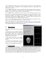
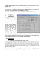
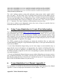
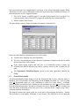
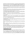
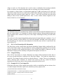
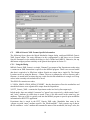
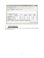
FITT2
Introduction to FITT Version 0.2.2
2013
Brian J. Soher
CONTENTS:
1. Introduction ........................................................................................................1
2. Overview of Main Widget .................................................................................1
3. The Viewer.........................................................................................................2
3.1.
General Usage ........................................................................................2
4. The Editor ..........................................................................................................3
4.1.
New Features .........................................................................................3
4.1.1. Gaussian Lineshape Model with Fixed T2 Values ..........................3
4.1.2. Fix Frequency Offset for Initial Values ...........................................4
4.1.3. Phase 0 Correction ...........................................................................4
4.1.4. Confidence Limits Selection ............................................................4
4.1.5. Prior Information Creation ...............................................................4
5. Using Vespa-Simulation to Create Prior Information .......................................5
6. Vespa-Simulation User Manual Appendix C ....................................................5
7. Acknowledgments............................................................................................12
1.
Introduction
This describes changes made in the second version of FITT. Most of the information in the
FITT_Help document still applies to this version.
Why is it version 0.2.2? – the previous version was listed as 1.7 and it is shown on the MIDAS
toolbar as “FITT2”; however, this was not in line with more typical open source software
versioning styles which typically list a “major”, “minor” and “revision” version number for a
software release. Because MIDAS is still in a BETA release mode (ie. Mostly stable, but under
development or known to have bugs), the major version number would typically be set to 0. So,
starting with FITT2, rather than calling it version 2.2, we released it with version number 0.2.2 to
bring it into a more standard nomenclature.
2.
The Main Widget
1) FITT requires that both a data file AND a
processing file be loaded at the same time. The
user is asked to select these when the
“LoadData”button is pressed.
1
2) The “Viewer”button brings up a new window that allows viewing the fit results and refitting
single voxels. This is a consolidation of what waspreviously known as “Image Thing” and
“Spectral View Control”.
3) The “Editor”button brings up a new widget that lists all processing parameters(replaces the
previous “Proc File Editor”). All changes of the processing settings are now immediately
applied, so will be used if a single-voxel fit is run from the Viewer.
4) The “DoFit” button starts the processing. The results will be automatically output to file if
that option is set in the processing parameters. If that option is not set the results can be saved to
file from the Viewer. Note, when a re-fitis donefrom the Viewer the results are NOT
automatically saved and the user must manually save any changes. This is to reduce file I/O
times to something that is not irritating in an interactive session.
5) The “Core” widget field(s) at the bottom of the main widget indicates how many CPU cores
will be used to fit the data and whether the core is Idle or Executing.
FITT2 works under the free Virtual Machine IDL license; however, as this doesn’t allow
multicore processing only a single thread is used, with longer processing times, and the section
of the widget showing the core status will not be shown.
3.
The Viewer
This widget consists of three main sections as
follows:
1) Tab notebook at top left contains options for
general navigation and control, less frequently
used options, settings for viewing and
changing the Mask, viewing the data header
and options for printing results.
2) The Map Canvas (lower left) displays
metabolite maps with the option for Mask
overlays.
3) The Plot Canvas (right) displays up to four
spectral plots each of which can be configured
to show a variety of single and overlay data.
3.1. General Usage
1) Mouse Operations -Left clicking on a voxel in the Map will cause the Plot to update to the
x,y,z voxel location. Right click and drag on Map tochange the intensity level the image. A Left
click and drag in the plot window will display a range with red cursors that will zoom in. A Left
click in place on the Plot will redisplay the full plot. Right click and drag will display a range of
yellow reference cursors that remain visible. The Area shown in the status bar is calculated
between the reference cursors. Middle button click and drag will phase the current voxel
2
2) Status Bar at bottom will display information regarding the mouse position and data values
under the cursor.
3) Resizing the entire widget frame will increase the size of the Plot window only.
4) Users can reset fit results for a single voxel using the ZeroVoxel button. Or they can reset the
entire results set using the Output→ZeroFittResults menu option.
5) Fit results can be manually saved to file using Output→SaveFittResultsmenu option.
4.
The Editor
The Editor widget replaces the
“Proc File Editor”, and contains
several tabs thateach contain a
subset of the fullfitting
parameterset.
For
most
parameters, the editor changes
the values of the parameters
currently loaded into memory,
but not the values in the file
originally loaded, and thus
these changes will immediately
be seen in any fits if the
ReFitVox button is hit on the
Viewer.
Examples
of
parameters
that
do
not
immediately change are Mask
source. Parameters like these are only updated on hitting the “DoFit” button in the Main
Window.Note that redoing a fit, either for the whole dataset or from the Viewer, will use the
current processing settings but will NOT save them to the processing file.To save the current
settings the ProcFile will have to be saved usingFile→Save Process File.
4.1. New Features
4.1.1. Gaussian Lineshape Model with Fixed T2 Values
For fitting of in vivo data the SNR is frequently not sufficient to support robust fitting of a Voigt
(Lorentz-Gauss) lineshape and therefore a Gaussian lineshape is recommended. However, a
Lorentzian lineshape component is still evident, which can differ substantially between creatine
and NAA. In the widget shown above is a new section that enables a fixed T2 value to be
entered for each metabolite. To force a Gaussian lineshape a large T2 value would be used, and
the values default to 1000 ms.
The value of the T2s used is not anticipated to be critical and a value that represents an average
of grey- and white-matter is suggested. The following papers report brain metabolite T2s at 3T:
3
Ganji SK, Banerjee A, Patel AM, Zhao YD, Dimitrov IE, Browning JD, Brown ES, Maher
EA, Choi C. T2 measurement of J-coupled metabolites in the human brain at 3T. NMR
Biomed 2012;25(4):523-529.
Mlynarik V, Gruber S, Moser E. Proton T1 and T2 relaxation times of human brain
metabolites at 3 Tesla. NMR Biomed 2001;14(5):325-331.
Kirov, II, Fleysher L, Fleysher R, Patil V, Liu S, Gonen O. Age dependence of regional
proton metabolites T2 relaxation times in the human brain at 3 T. MagnReson Med
2008;60(4):790-795.
Zaaraoui W, Fleysher L, Fleysher R, Liu S, Soher BJ, Gonen O. Human brain-structure
resolved T(2) relaxation times of proton metabolites at 3 Tesla. MagnReson Med
2007;57(6):983-989.
Based on these reports here are some suggested values for 3T: NAA = 260; Cre = 160; Cho =
230; mI = 200; Glu=180; Water = 85.
4.1.2. Fix Frequency Offset for Initial Values
Also shown in the widget shown above is a checkbox by each metabolite to “Use DB ppm
values”. If checked, this will force the program to use the prior information of the peak
frequency offsets when estimating initial values. If unchecked, the maximum value over a small
frequency range will be used.We have used this in some data sets to improve starting values for
lactate where there are significant baseline contributions surrounding the lactate signal that can
fool the peak search algorithms in the initial values routines.
4.1.3. Phase 0 Correction
Two options are now included to apply a zero-order phase correction to the data. The first is in
the “Initial” tab, and allows applying a zero-order phase correction to the data and then
rerunning the initial values estimation. The second option is in the “Global” tab, and includes
options to unwrap the zero-order phase function and then apply this to the data. This option has
been found to improve fitting in cases where peaks are phased close to 180 degrees. Note this
option will not apply the phase correction to the spectral data stored on disk, but this can be done
using the setting in the “Output” tab, to “Apply Phase01 values to Original Data”.
4.1.4. Confidence Limits Selection
The calculation of confidence limits can be quite time consuming, so an option has been added in
the “QA” tab to only calculate selected values instead of all parameters.
4.1.5. Prior Information Creation
MIDAS-FITT2 reads an XML file that contains prior information about the metabolites used in
the fitting model. An example of a text file (could be any name, but metabolites.xml is one
reasonable example) showing three metabolites, NAA, creatine and choline is shown below.
<PRIOR_METABOLITE_INFORMATION>
<param value="choline++0++0++0++0++3.1850000++9.0000000++1.9575600e-015" name="fitt_PriorLine001"/>
<param value="creatine++0++0++0++0++3.0270000++3.0000000++-5.3074000e-016" name="fitt_PriorLine002"/>
<param value="n-acetyl-aspartate++0++0++0++0++2.008000++3.00000++8.2668400e-016" name="fitt_PriorLine003"/>
<param value="n-acetyl-aspartate++0++0++0++1++2.3644400++0.13678200++-27.715700" name="fitt_PriorLine004"/>
<param value="n-acetyl-aspartate++0++0++0++2++2.4404700++0.10923800++64.185600" name="fitt_PriorLine005"/>
<param value="n-acetyl-aspartate++0++0++0++3++2.4911700++0.36175400++-100.53400" name="fitt_PriorLine006"/>
<param value="n-acetyl-aspartate++0++0++0++4++2.5672000++0.38643300++56.696200" name="fitt_PriorLine007"/>
4
<param value="n-acetyl-aspartate++0++0++0++5++2.6112500++0.34797200++-84.292700" name="fitt_PriorLine008"/>
<param value="n-acetyl-aspartate++0++0++0++6++2.6464100++0.40218600++128.61300" name="fitt_PriorLine009"/>
<param value="n-acetyl-aspartate++0++0++0++7++2.7379800++0.14213500++-158.19000" name="fitt_PriorLine010"/>
<param value="n-acetyl-aspartate++0++0++0++8++2.7731400++0.10540700++119.90000" name="fitt_PriorLine011"/>
</PRIOR_METABOLITE_INFORMATION>
The “value” attribute contains a string with eight parts: unique_name, index1, index2, index3,
ppm, area, phase. The three index values are integers and not currently used in MIDAS, but are
reserved for future expansion. The unique_name value is a unique text name for the metabolite.
The area, ppm and phase values are floating point value. Area is normalized to the number of
spins in the metabolite. Phase values are in degrees. All values in the “value” string are separated
by “++” characters. The “name” attribute is used internally to sort prior values.
Users can use whatever prior information sources they want, so long as it provides data in a
format that matches the required XML format.
5.
Using Vespa-Simulation to Create Prior Information
The Vespa-Simulation program (http://scion.duhs.duke.edu/vespa)is recommended to create the
prior information used in the FITT program. Vespa-Simulation allows you to create pulse
sequences using Python code that can access the GAMMA spectral simulation library. Using
these sequences, users can run spectral simulations and create prior metabolite information that
can be used as basis sets in FITT. Vespa-Simulation has an output utility that can save its results
to a file in both FITT 1.7 and FITT 0.2.x formats.
The VESPA program provides information on running the simulation. Here we make some
recommendations for using the Vespa-Simulation output utility to create prior information basis
sets for use in MIDAS:
1. In the Mixed Metabolite Output dialog, use the Scale widget on each metabolite entry to
ensure that the areas for all singlets are set appropriately. For example, if tCholine(which uses a
CH3 group) was used in a simulation, you should set the Scale value to 3.0, this will ensure that
the choline peak that is output has an area value corresponding to 9 protons, rather than the 3 that
was used to simulate it.
2. Use the Add Metabolite Mixture button to pop up another dialog that you can use to create a
mix of simulated metabolites. For example, you can create a mixture of NAA and NAAG using
this dialog by setting the relative NAA area to 1.0 and NAAG area to 0.15. You can similarly use
this to create Glx and other mixtures for your basis set.
6.
Vespa-Simulation User Manual Appendix C
For convenience, we include here the relevant sections from the Vespa-Simulation User Manual
Appendix C on how to output prior information for use in MIDAS 1.7 and 2.x
Appendix C. Mixed Metabolite Output
5
This section describes the implementation and usage of the Mixed Metabolite Output dialog.
This dialog is used to convert Simulation results into various third party readable file formats. At
the moment, there are five supported formats:
1. The GAVA format, so-called because it was part of the original GAVA program. It is
used extensively in the SITools/FITT program as metabolite prior information files.
2. MIDAS Generic XML format
The same dialog is used to output all formats; an example is shown below:
Please note the following requirements to access this widget:
You must have loaded at least one Experiment.
The active Experiment tab (if more than one Experiment is loaded) is the one for which
the third party files will be output.
If the output format requires that only one set of metabolite results is output (eg.
LCModel and jMRUI) then the loop indices currently selected in the Visualize tab are
used.
The Experiment→ThirdPartyExport…menu on the main application launches the
dialog.
C.1
General Functionality
The Mixed Metabolite Output dialog acts on the Experiment that is active when the dialog is
launched. The GUI reformats itself depending on the Format pull down list. GAVA format
saves all Experiment results (ie. every simulation for each set of loop values). LCModel,
jMRUI, MIDAS and Analysis Prior formats save all metabolites for only one set of loop values
from the selected Experiment. The indices selected in the active Experiment in the Visualize tab
when the dialog is launched are the ones used. This is indicated in the “Output Loop Values”
comment at the top of the dialog.
The Output Location into which results are saved can be selected using the Browse… button.
This selection is used slightly differently in each format. The differences will be discussed
6
specifically for each format in the sections below. A comment can be added in the dialog that is
included in all text output. The dialog defaults to listing all metabolites in the Experiment, but
these can be removed or put back in with the Add Metabolite and RemoveSelected buttons. The
Add Metabolite Mixture …button will pop up another small dialog in which you can design a
“mixture” of two or more metabolite results with different scaling factors. This will be described
in detail later. The Cancel button quits the dialog without performing any output. The OK button
outputs the described collection of metabolite results and mixtures to the indicated format and
Output Location.
For all formats, the dialog creates a header comment block that is prepended to all text files
being output. This header describes the Experiment and results/mixtures being output, and lists
the modifying parameters for metabolites and formulae for any mixtures.
The Metabolite and Mixed Metabolite Output List is a dynamic list that changes length as
entries are added or deleted. Each row in this list is a result that will be saved upon output. The
widgets in each row affect the way the results are output as defined below:
•Checkbox – is used to select rows to delete from the output list, but otherwise does not affect
whether a given metabolite/mixture is output or not. All rows present when you hit OK are used
to create the output.
•Metabolite List – drop list, is used to select which metabolite to output. The other widget
settings in this row modify the results for the selected metabolite/mixture. It is possible to have
two or more of the same metabolite selected for output. The only requirement is that they have
unique strings in the Unique Abbreviation field.
•Unique Abbreviation – text field, a unique string used to identify this output row. In LCModel
and jMRUI Data Text, this is the metabolite output filename. In GAVA Text, this is the first
column metabolite name string.
•Scale – floatspinfield, should contain a float value and should be positive. The area values for
all lines in an Experiment Simulation result are multiplied by this scale value before being
output.
•Shift – floatspinfield, should contain a floating point PPM value and can be positive or
negative. This shift value is added to all ppm values for all lines in an Experiment Simulation
result before being output.
Range Start and Range End – floatspin fields, should contain floating point ppm values. These
values default to the min/max ppm values displayed for the active Experiment. They can be set
narrower to filter the results that are output. Only the Experiment Simulation lines that lie
between the start and end ppm range will be included in the output files. Each row can have a
different range. Again, all these settings are saved in the header comment block on output.
Add Metabolite Mixture …Button
This button allows users to add a “mixture” result to the Output list. Each mixture can consist of
two or more metabolites, each with a different mixture scaling factor (as opposed to the Scale
field on the main dialog). The Mixed Metabolite Designer widget is shown below. The user has
to specify a Unique Name string that is different from all other strings in the Abbreviation
column in the main dialog. The user can click on the Add Metabolite and Remove Selected
(with a check box selected) buttons to change the number of metabolites in the mix. The drop list
7
widget in each row of the dynamic list is used to select a metabolite from existing metabolite
results. A mixture can contain metabolites that are not being saved in the main dialog.
For example, as shown below, an Experiment might have GABA and lactate in its results list
drop down widget. But the user could remove both GABA and lactate from the list in the main
widget, and create a mixture called “gaba+lac” with a 1:5 ratio. This would show up in the main
dialog as shown in the second figure below. Note. A more realistic mixture might be to mix
NAA to NAAG in a 1:0.05 mixture.
Mixture Creation Caveats:
The Metabolite drop list is populated only with the concatenation of all full metabolite names (in
this case “gaba+lactate”) as a reminder of what the mixture contains. When metabolite names get
long, sometimes these cannot be fully seen in this widget. Widening the dialog can make these
more visible.
The scales set in the mixture design dialog and main mixed output dialog are cumulative. E.g. if
you create a mixture of NAA+NAAG at 1:0.05 in the designer, and then set the Scale value in
the main dialog to 3.0, then the actual multiplier for NAA line areas will be 3.0 and NAAG line
areas will be 0.15.
C.2
GAVA Text Format Specific Information
The first figure in this section shows the Mixed Metabolite Output dialog configured for the
GAVA Text format output. The main difference in this configuration is that there are no Format
Specific Parameters in the middle the dialog (as for LCModel and jMRUI). Otherwise, the top
and bottom widgets perform similarly to the general descriptions in section C.1.
C.2.1 Using the Dialog
Since GAVA Text format is a simple “flattened” text output of the Experiment results, there is
no user-set header data that is required to be filled into widgets. The results are output into a
single file. The Output Location can be set using the Browse… button. The user is prompted to
select a directory and a filename. As stated in the section at the top, results for selected
metabolites in for all loop values in the currently selected tab will be saved.
C.2.2 Example GAVA Text Output File
Following in the steps of the example shown above with two metabolites and one mixture, here
is a short example of the data output to the simulation_mixed_output.txt file
;Vespa-Simulation Mixed Metabolite Output
;
;Output Path/Filename = C:\bsoher\temp\simulation_mixed_output.txt
;Output Loop Values = All loops will be saved for this format
;Output Comment
;---------------------------------------------------------------------------
8
;
;
;Experiment Information
;--------------------------------------------------------------------------;--- Experiment 91291fb0-95d0-4e62-b95e-028d96d5e853 --;Name: Example SpinEcho multi-TE
;Public: True
;Created: 2010-10-11T11:22:17
;Comment (abbr.): example of a spin-echo experiment at 3T
;PI: bjs
;b0: 128.000000
;Peak Search PPM low/high: 0.000000 / 10.000000
;Blendtol. PPM/phase: 0.001500 / 50.000000
;Pulse seq.: 2e9c8f33-06d4-4934-ae2b-199b605fe98a (Spin-Echo)
;0 User static parameters:
;7 Metabolites: choline-truncated, creatine, gaba, glutamate, lactate, myo-inositol, n-acetylaspartate
;98 Simulations: (not shown)
;
;Metabolite Formatting Information
;--------------------------------------------------------------------------;Name=choline-truncated Abbr=choline-truncated Scale=1.0 Shift=0.0 PPM Start=-3.10487060547 PPM
End=12.5125
;Name=creatine Abbr=creatine Scale=1.0 Shift=0.0 PPM Start=-3.10487060547 PPM End=12.5125
;Name=gaba+lactateAbbr=gaba+lac Scale=1.0 Shift=0.0 PPM Start=-3.10487060547 PPM End=12.5125
; Mixture of [metab*scale] = gaba*1.0 + lactate*5.0
;
;Simulation Spectral Results
;--------------------------------------------------------------------------choline-truncated 10.0
0.0
0.0
0
3.185 3.0
-9.93923337957e-16
creatine 10.0
0.0
0.0
0
3.027 3.0
-7.95138670366e-16
creatine 10.0
0.0
0.0
1
3.913 2.0
-4.96961668979e-17
creatine 10.0
0.0
0.0
2
6.649 1.0
9.93923337957e-17
gaba+lac
10.0
0.0
0.0
0
1.64314237348 6.82464923377e-05
46.1587697321
gaba+lac
10.0
0.0
0.0
1
1.76022959161 0.0599190291344
47.6446766073
…
In the GAVA Text format, lines starting with a semicolon are ignored as comments. Thus the
prepended header comment block starts all lines with “;”. The actual data starts on the final 6
lines shown, with a tab-delineated layout. Each row of data in the file contains the name of the
metabolite, the loop1 value, the loop2 value, the loop3 value, the transition table line number for
the metabolite, the ppm value, area value and phase value for each spectral line in the metabolite
Simulation result. For choline and creatine, these are only 1 and 3 lines respectively. But, for
other multiplet resonance metabolite results, such as the gaba+lac mixture, this can run to 10s to
100s of lines of data. And if the Experiment had more that one loop in it, the first set of results is
written out for all metabolites, then the next loop value for all metabolites, and so on. In the
example above with two metabolites and one mixture output for a spin-echo pulse sequence
Experiment with 10 TE settings, there were 2838 lines of results in the final file.
9
C.5
MIDAS Generic XML Format Specific Information
The following figure shows the Mixed Metabolite Output dialog configured MIDAS Generic
XML format output. The main difference in this configuration is that there are no Format
Specific Parameters in the middle the dialog (as for LCModel and jMRUI). Otherwise, the top
and bottom widgets perform similarly to the general descriptions in section C.1.
C.5.1 Using the Dialog
MIDAS Generic XML format is a simple “flattened” text output of the Experiment results using
a variant on an XML format that is specific to the MIDAS program. There is no user-set header
data that is required to be filled into widgets. Results are output into a single file. The Output
Location can be set using the Browse… button. The user is prompted to select a directory and a
filename. As stated in the section at the top, results for selected metabolites in a single set of loop
values in the currently selected tab will be saved.
This XML file contains two nodes,
1) VESPA_SIMULATION_MIDAS_EXPORT - has the description of how the metabolites and
metabolite mixtures were organized for output from the Experiment.
2) FITT_Generic_XML - contains the Experiment results in a line-by-line output style.
In both nodes, there are multiple "comment" or "param" tags, respectively, which contain "name"
and "value" attributes in which data is stored. There is no data stored in the actual tag, just
attributes. This type of file is typically read into the MIDAS program to provide prior metabolite
information for the FITT2 application.
Experiment data is stored in the FITT_Generic_XML node. Metabolite data starts in the
<param> tag with “name” attribute equal to “fitt_PriorLine00001”. Each <param> tag of data in
the file contains a “value” attribute that contains the name of the metabolite, the loop1 value, the
10
loop2 value, the loop3 value, the transition table line number for the metabolite, the ppm value,
area value and phase value for each spectral line in the metabolite Simulation result. These are
all stored in one text string separated by “++” symbols. For choline and creatine, these are only 1
and 3 lines respectively. But, for other multiplet resonance metabolite results, such as the
gaba+lac mixture, this can run to 10s to 100s of lines of data.
C.5.2 Example MIDAS Generic XML Output File
Following in the steps of previous examples (with two metabolites and one mixture), here is a
short example of the data output to the midas_output.xml file
<FITT_Generic_XMLCreation_date="2011-03-08" Creation_time="11:55:32">
<VESPA_SIMULATION_MIDAS_EXPORT>
<comment line="line0000" value="Vespa-Simulation Mixed Metabolite Output" />
<comment line="line0001" value="" />
<comment line="line0002" value="Output Path/Filename = C:\bsoher\code\repository_svn\vespa\simulation\midas_output.xml" />
<comment line="line0003" value="Output Loop Values = All loops will be saved for this format" />
<comment line="line0004" value="Output Comment" />
<comment line="line0005" value="---------------------------------------------------------------------------" />
<comment line="line0006" value="" />
<comment line="line0007" value="" />
<comment line="line0008" value="Experiment Information" />
<comment line="line0009" value="---------------------------------------------------------------------------" />
<comment line="line0010" value="---Experiment 92adae26-137e-48ce-8c35-02905bb5cfd5 ---" />
<comment line="line0011" value="Name: Example PRESS_Ideal multi-TE" />
<comment line="line0012" value="Public: True "/>
<comment line="line0013" value="Created: 2011-01-24T11:01:16" />
<comment line="line0014" value="Comment (abbr.): Example of a PRESS experiment at 3T usin" />
<comment line="line0015" value="PI: bjs" />
<comment line="line0016" value="b0: 128.000000" />
<comment line="line0017" value="Peak Search PPM low/high: 0.000000 / 10.000000" />
<comment line="line0018" value="Blend tol. PPM/phase: 0.001500 / 50.000000" />
<comment line="line0019" value="Pulse seq.: 0b3db82e-d04b-4719-b8f9-95f1153f0d50 (PRESS Ideal)" />
<comment line="line0020" value="0 User static parameters:" />
<comment line="line0021" value="7 Metabolites: choline,creatine,gaba,glutamate,lactate,myo-inositol,n-acetylaspartate" />
<comment line="line0022" value="98 Simulations: (not shown)" />
<comment line="line0023" value="" />
<comment line="line0024" value="Metabolite Formatting Information" />
<comment line="line0025" value="---------------------------------------------------------------------------" />
<comment line="line0026" value="Name=choline Abbr=choline Scale=1.0 Shift=0.0 PPM Start=-3.10487 PPM End=12.5125" />
<comment line="line0027" value="Name=creatine Abbr=creatine Scale=1.0 Shift=0.0 PPM Start=-3.10487060547 PPM End=12.5125" />
<comment line="line0028" value="Name=gaba+lactateAbbr=gaba+lac Scale=1.0 Shift=0.0 PPM Start=-3.10487 PPM End=12.5125" />
<comment line="line0029" value="Mixture of [metab*scale] = gaba*1.0 + lactate*1.0" />
</VESPA_SIMULATION_MIDAS_EXPORT>
<PRIOR_METABOLITE_INFORMATION>
<param name="fitt_PriorLine00001" value="choline-truncated++10.0++30.0++0.0++0++3.185++3.0++3.2680199352e-13" />
<param name="fitt_PriorLine00002" value="creatine++10.0++30.0++0.0++0++3.027++3.0++2.85844069302e-13" />
<param name="fitt_PriorLine00003" value="creatine++10.0++30.0++0.0++1++3.913++2.0++1.90976157368e-13" />
<param name="fitt_PriorLine00004" value="creatine++10.0++30.0++0.0++2++6.649++1.0++4.77915613015e-13" />
<param name="fitt_PriorLine00005" value="gaba+lac++10.0++30.0++0.0++0++1.30216386911++6.56750777889e-05++-138.531997369" />
<param name="fitt_PriorLine00006" value="gaba+lac++10.0++30.0++0.0++1++1.39807431416++8.34965132792e-05++94.719201079" />
...
...
<param name="fitt_PriorLine00182" value="gaba+lac++10.0++30.0++0.0++177++4.17942135846++0.117527687393++-149.811478877" />
</PRIOR_METABOLITE_INFORMATION>
</FITT_Generic_XML>
11
7.
Acknowledgments
This program was developed by Brian J. Soher. This work was supported by NIH grant EB00822
under the MIDAS project.
12