1
Marco Antonio Espinoza Sanchez
Candidate
Electric and Computer Engineering
Department
This thesis is approved, and it is acceptable in quality and form for publication:
Approved by the Thesis Committee:
Wei Wennie Shu
, Chairperson
Thomas P. Caudell
Marios S. Pattichis
i
Design & Implementation of a Pivot Shift
Prototype for Quantitative Analysis
by
Marco Antonio Espinoza Sanchez
B.S., Chihuahua Institute of Technology, 2011
THESIS
Submitted in Partial Fulfillment of the
Requirements for the Degree of
Master of Science
Computer Engineering
The University of New Mexico
Albuquerque, New Mexico
May, 2015
©2015, Marco Antonio Espinoza Sanchez
iii
Dedication
To my family and friends which always supported me through the University years.
I probably wouldn’t be writing this thesis without their help.
iv
Acknowledgments
I would like to thank and sincerely acknowledge my Thesis advisor Dr. Wei Wennie
Shu for the guidance and support provided during the realization of this work. I
would also like to thank Dr. Thomas P. Caudell and Dr. Marios S. Pattichis for
being part of the thesis evaluation committee.
As well I would like to express my gratitude to CONACYT ( Consejo Nacional
de Ciencia y Tecnologı́a) for all the support to make this happen.
Special thanks to my friend Engineer Jose Dı́az for the help with the design and
support of the prototype and to the medical staff leaded by Edmundo Berumen M.D.
and Carlos Vega M.D. collaborating on the patient trials.
v
Design & Implementation of a Pivot Shift
Prototype for Quantitative Analysis
by
Marco Antonio Espinoza Sanchez
B.S., Chihuahua Institute of Technology, 2011
M.S., Computer Engineering, University of New Mexico, 2015
Abstract
This thesis presents the utilization of a portable medical device intended to help
in the diagnosis of the Anterior Cruciate Ligament(ACL) knee injury. The prototype
consists of an embedded system integrated with various sensors including accelerometers and gyroscopes to provide force, orientation, and acceleration measurement. The
prototype has been used to quantify the results of a medical test called pivot shift
which tests the dynamic stability of the patient’s knee. With the initial prototype
built, limited clinical trials were conducted. Two schemes (metric based classification
and k nearest neighbors) have been applied to the data set to empirically learn and
judge ACL diagnosis.
vi
Contents
List of Figures
ix
List of Tables
xiii
1 Introduction
1
1.1
How the project got started . . . . . . . . . . . . . . . . . . . . . . .
1
1.2
The ACL Injury . . . . . . . . . . . . . . . . . . . . . . . . . . . . . .
2
1.3
Diagnosis . . . . . . . . . . . . . . . . . . . . . . . . . . . . . . . . .
4
1.3.1
Knee Arthroscopy . . . . . . . . . . . . . . . . . . . . . . . . .
4
1.3.2
Non-Invasive Techniques . . . . . . . . . . . . . . . . . . . . .
5
2 The Pivot Shift Prototype: Hardware Design
2.1
2.2
12
Arduino . . . . . . . . . . . . . . . . . . . . . . . . . . . . . . . . . .
12
2.1.1
Arduino Mini Pro 328 . . . . . . . . . . . . . . . . . . . . . .
13
MEMS:Accelerometer and Gyroscope . . . . . . . . . . . . . . . . . .
15
2.2.1
16
Accelerometers . . . . . . . . . . . . . . . . . . . . . . . . . .
vii
Contents
2.3
2.2.2
Gyroscope . . . . . . . . . . . . . . . . . . . . . . . . . . . . .
18
2.2.3
MMA7361LC: Three Axis Low-g Accelerometer . . . . . . . .
20
2.2.4
LSM9DS0: 3D Accelerometer/Gyroscope module . . . . . . .
27
2.2.5
I2 C Protocol . . . . . . . . . . . . . . . . . . . . . . . . . . . .
29
2.2.6
Getting data from the LSM9DS0 . . . . . . . . . . . . . . . .
31
The Prototype . . . . . . . . . . . . . . . . . . . . . . . . . . . . . . .
36
3 The Pivot Shift Prototype: Software Design
41
3.1
Processing . . . . . . . . . . . . . . . . . . . . . . . . . . . . . . . . .
41
3.2
The Basics . . . . . . . . . . . . . . . . . . . . . . . . . . . . . . . . .
43
3.3
The Pivot Shift Software . . . . . . . . . . . . . . . . . . . . . . . . .
45
3.3.1
The Coding . . . . . . . . . . . . . . . . . . . . . . . . . . . .
46
3.3.2
Beginning the test . . . . . . . . . . . . . . . . . . . . . . . .
49
3.3.3
During the test . . . . . . . . . . . . . . . . . . . . . . . . . .
51
3.3.4
From angular velocity to angular displacement . . . . . . . . .
56
3.3.5
Ending the test and storing data . . . . . . . . . . . . . . . .
60
4 Clinical Trials
63
5 Data Acquisition and Analysis
67
5.1
First glance at graphs and PyPlotter . . . . . . . . . . . . . . . . . .
68
5.2
Interpretation of Graphical Data
72
viii
. . . . . . . . . . . . . . . . . . . .
Contents
5.3
Adjusting Left leg X axis readings . . . . . . . . . . . . . . . . . . . .
76
5.4
Transforming to G’s . . . . . . . . . . . . . . . . . . . . . . . . . . .
78
5.5
Tools and Packages used . . . . . . . . . . . . . . . . . . . . . . . . .
80
5.6
Data Statistics . . . . . . . . . . . . . . . . . . . . . . . . . . . . . .
82
5.6.1
Left and Right legs statistics . . . . . . . . . . . . . . . . . . .
87
Classifying patients from data . . . . . . . . . . . . . . . . . . . . . .
89
5.7.1
Metric classifiers . . . . . . . . . . . . . . . . . . . . . . . . .
90
5.7.2
Non parametric classification: K Nearest Neighbors . . . . . .
95
5.7
6 Conclusion and Future Work
102
6.1
Limitations and Future Work . . . . . . . . . . . . . . . . . . . . . . 102
6.2
Conclusion . . . . . . . . . . . . . . . . . . . . . . . . . . . . . . . . . 106
A Arduino and Processing Code
108
References
109
ix
List of Figures
1.1
Normal knee anatomy, front view . . . . . . . . . . . . . . . . . . . .
3
1.2
Frontal view of a knee with ACL injury . . . . . . . . . . . . . . . .
4
1.3
Arthroscopy equipment and setup on patient’s knee . . . . . . . . .
5
1.4
MRI: Acute anterior ligament tear . . . . . . . . . . . . . . . . . . .
7
1.5
KT-1000 test measuring anterior-posterior knee translation . . . . .
8
1.6
Clinical assessments for the ACL diagnosis . . . . . . . . . . . . . .
9
1.7
Pivot Shift test . . . . . . . . . . . . . . . . . . . . . . . . . . . . . .
10
2.1
Arduino Mini Pro . . . . . . . . . . . . . . . . . . . . . . . . . . . .
14
2.2
MEMS components diagram . . . . . . . . . . . . . . . . . . . . . .
16
2.3
Piezoelectric accelerometer, spring moves as acceleration forces act
upon the sensor, producing a voltage proportional to that force . . .
2.4
2.5
17
Three-Axis accelerometer LIS331DLHXY used in iPhone 4 in detail,
micromachined proof mass interleaved with capacitive sensors . . . .
19
MEMS gyroscope submitted to Coriolis effect . . . . . . . . . . . . .
20
x
List of Figures
2.6
MEMS gyroscope submitted to angular motion . . . . . . . . . . . .
21
2.7
MEMS gyroscope submitted to linear acceleration . . . . . . . . . .
21
2.8
MMA7361LC analog accelerometer breakout board showing respective directions for each axis . . . . . . . . . . . . . . . . . . . . . . .
22
2.9
MMA7361LC and Arduino connection diagram . . . . . . . . . . . .
22
2.10
Reading the output of the MMA7361LC accelerometer resting at
horizontal position . . . . . . . . . . . . . . . . . . . . . . . . . . . .
25
2.11
The effect of gravity on accelerometer readings . . . . . . . . . . . .
26
2.12
I2 C signals, showing the start condition, address and data frames,
,and stop condition . . . . . . . . . . . . . . . . . . . . . . . . . . .
2.13
Schematic diagram of two LSM9DS0’s connected to an Arduino Mini
board under I2 C . . . . . . . . . . . . . . . . . . . . . . . . . . . . .
2.14
31
32
Reading the output of the LSM9DS0 accelerometer resting at horizontal position . . . . . . . . . . . . . . . . . . . . . . . . . . . . . .
36
2.15
MRI, complete tear of ACL ligament . . . . . . . . . . . . . . . . . .
37
2.16
MRI, partial tear of ACL ligament . . . . . . . . . . . . . . . . . . .
38
2.17
The pivot shift tester, one sensing module located in the tibia and
the second one in the femur . . . . . . . . . . . . . . . . . . . . . . .
39
3.1
Simple application using Processing . . . . . . . . . . . . . . . . . .
44
3.2
High level algorithm for pivot shift software . . . . . . . . . . . . . .
45
3.3
A selection of controllers available with ControlP5 library . . . . . .
47
xi
List of Figures
3.4
User interface for the pivot shift tester . . . . . . . . . . . . . . . . .
48
3.5
Pivot Shift UI, dual layout presentation . . . . . . . . . . . . . . . .
54
3.6
Sample acceleration graph: x axis in red, y axis green, and z axis in
blue . . . . . . . . . . . . . . . . . . . . . . . . . . . . . . . . . . . .
56
3.7
LSM9DS0 module: directions for acceleration and angular rates . . .
57
3.8
Sample test using angular velocity . . . . . . . . . . . . . . . . . . .
58
3.9
Sample test using angular displacement . . . . . . . . . . . . . . . .
59
3.10
Sample test showing axes signals individually . . . . . . . . . . . . .
61
3.11
Sample test showing the magnitude for acceleration and angular displacement . . . . . . . . . . . . . . . . . . . . . . . . . . . . . . . .
62
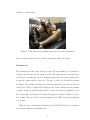
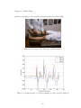
4.1
Prototype used during pivot shift maneuver . . . . . . . . . . . . . .
66
4.2
Graph showing acceleration output per axis from pivot shift test . .
66
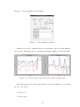
5.1
Pivot shift plot analyzer . . . . . . . . . . . . . . . . . . . . . . . . .
69
5.2
Patient graphs: left leg (left side), right leg (right side)
69
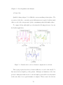
5.3
Patient’s side to side acceleration comparison for each axis
. . . . .
70
5.4
Side to side comparison for X axis in four different patients . . . . .
72
5.5
The pivot shift movement step by step, bottom describes positive
. . . . . . .
directions for acceleration on each of the axis . . . . . . . . . . . . .
74
5.6
Interpretation of the maneuver . . . . . . . . . . . . . . . . . . . . .
75
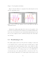
5.7
Compensation of internal tibial rotation for X axis readings . . . . .
77
xii
List of Figures
5.8
Side to side X axis comparison: left side with original data, right side
compensating rotation . . . . . . . . . . . . . . . . . . . . . . . . . .
78
5.9
Histograms for complete dataset: a) X axis, b) Y axis, c) Z axis . . .
83
5.10
Mean, median and sd for complete data set by axis . . . . . . . . . .
85
5.11
Mean, median and sd by healthy and ACL patients
. . . . . . . . .
85
5.12
Taking the median of the maximum values . . . . . . . . . . . . . .
86
5.13
Left legs: mean, median and sd for ACL and healthy patients . . . .
93
5.14
Right legs: mean, median and sd for ACL and healthy patients . . .
94
5.15
From (acceleration, time) to (X,Z) sample points . . . . . . . . . . .
96
5.16
XZ datasets corresponding to right leg . . . . . . . . . . . . . . . . .
97
5.17
Creating subsets of the healthy class with equal size of ACL class . .
98
5.18
Testing and training set examples . . . . . . . . . . . . . . . . . . .
99
5.19
Classification results for patient file P12PD . . . . . . . . . . . . . . 100
6.1
XBee module implementation . . . . . . . . . . . . . . . . . . . . . . 103
6.2
Disparity in sample size and beginning of test . . . . . . . . . . . . . 105
6.3
Recent test after software changes, 3/14/15 . . . . . . . . . . . . . . 105
xiii
List of Tables
2.1
Zero-g voltage taken from data-sheet and device testing . . . . . . .
25
2.2
LSM9DS0 Accelerometer characteristics . . . . . . . . . . . . . . . .
27
2.3
LSM9DS0 Gyroscope characteristics . . . . . . . . . . . . . . . . . .
28
2.4
I2 C terminology . . . . . . . . . . . . . . . . . . . . . . . . . . . . .
30
3.1
Conversion from angular velocity to angular displacement in X axis .
60
5.1
Patients distribution . . . . . . . . . . . . . . . . . . . . . . . . . . .
82
5.2
Summary statistics for X, Y and Z data for all patients . . . . . . .
84
5.3
Summary for X, Y and Z data for patients by groups . . . . . . . . .
84
5.4
Maximum and minimum acceleration metrics . . . . . . . . . . . . .
87
5.5
Example table showing maximum and minimum values for 5 patients 87
5.6
Summary statistics for X, Y and Z in left and right legs . . . . . . .
88
5.7
XYZ summary for patients by groups, left and right legs . . . . . . .
88
5.8
Maximum and minimum values for patients by groups, left and right
legs . . . . . . . . . . . . . . . . . . . . . . . . . . . . . . . . . . . .
xiv
89
List of Tables
5.9
Magnitude metrics summary for healthy and ACL patients . . . . .
90
5.10
Results of different metric based classification approaches . . . . . .
92
5.11
MagnitudeXZ metrics summary for healthy and ACL patients . . . .
94
5.12
XZ Magnitude metric classification results . . . . . . . . . . . . . . .
95
5.13
KNN results for Left leg . . . . . . . . . . . . . . . . . . . . . . . . . 100
5.14
KNN results for Right leg . . . . . . . . . . . . . . . . . . . . . . . . 101
5.15
KNN: missclassifications rates by groups . . . . . . . . . . . . . . . . 101
6.1
Variability in sample size from test to test . . . . . . . . . . . . . . . 104
xv
Chapter 1
Introduction
This Thesis is based on the implementation of a previously design pivot shift prototype and its tests results in patients trails. The project consisted of an interdisciplinary collaboration between engineering and medical professionals.
The patient trials took place in Chihuahua, Mexico with collaboration of Edmundo Berumen M.D. and Carlos Vega M.D. at the Christus Muguerza del Parque
Hospital between May 2013 and May 2014.
1.1
How the project got started
Part of the work showed in this Thesis backs from early 2013 before my arrival
to UNM. Everything started with a call from a friend MD. Carlos Vega, that at
that moment was working on some orthopedical research with regards of the ACL
(anterior cruciate ligament) knee injury. In that call he mentioned got an idea of
an electronics project that i may could possibly be interested in. He started talking
about how he was working on this routine test called pivot shift and the problems it
had with the equipment that he was using to measure the results. Then he finally
1
Chapter 1. Introduction
said “could be a way to measure the movement or the force used during the test??,
something to see the results on a PC..”. After that I contacted my friend also
an electronics engineer Jose Diaz, got together, bought some microcontrollers and
sensors and started playing with the project.
1.2
The ACL Injury
Knee injuries comprise about 55% of all sports injuries. Out of those, ACL (anterior
cruciate ligament) tear represents one of the most common ones. Athletes involved
in high demand disciplines like basketball, soccer, and football are more likely to
develop this injury.
Briefly analyzing the knee anatomy the main three bones being part of the knee:
• Femur
• Patella
• Tibia
These bones connect to each other by ligaments to keep knee stability and protection
limiting the movement. These ligaments can be described as:
• Collateral ligament. These ligaments can be found on the sides of the knees.
The lateral collateral is located on the outside while the medial collateral on
the inside. Their function consist on controlling the knee sideways motion and
prevent unusual movement.
• Cruciate ligaments. Ligaments that are found inside the knee joint. The posterior cruciate ligament being located on the back while the anterior posterior
2
Chapter 1. Introduction
lies on the frontal part of the knee. They are responsible of the back and forth
dynamic of the knee.
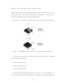
Figure 1.1: Normal knee anatomy, front view
Figure 1.1 shows the anatomy of a healthy knee where it can be seen how the
ACL runs in the middle of the knee in diagonal direction, because of this prevents
the tibia from sliding or moving out in front of the femur [1].
In the other hand figure 1.2 exposes a knee with the ACL injury, which among
other things can be caused by:
• Direct impact or collision on one side of the knee
• Sudden stop of movement
• Overextend the knee joint
• Quick stop of motion and change direction while turning, landing from a jump
or running.
• Slowing down while running
• Landing from a jump incorrectly
3
Chapter 1. Introduction
Figure 1.2: Frontal view of a knee with ACL injury
1.3
Diagnosis
Once there is the suspicion of an ACL tear, Doctors often use several techniques
to determine if in fact an injury exist. There are invasive techniques like the knee
arthroscopy and multiple non-invasive that can identified in two main groups, one
being imaging tests like Radiography, CT scans and MRI, and the ones called routine
tests or medical assessments including lachman, pivot shift and drawer tests.
1.3.1
Knee Arthroscopy
Knee arthroscopy is a minimally invasive technique that allows orthopedic surgeons
to assess and treat several conditions affecting the knee joint. The procedure consist
of a small incision in the vicinity of the affected joint. Then a tiny camera (around
size of a pencil) is inserted along with fiber optics to provide light source. The camera
transmits the images in real time to a monitor in the operating room, this way the
specialist can gain multiple views of the joint area.
The surgeon can use this technique to assess, repair or remove damaged tissue,
to do so, other small surgical equipment is inserted via a secondary incision around
4
Chapter 1. Introduction
Figure 1.3: Arthroscopy equipment and setup on patient’s knee
the knee. Aside from the invasive nature of this technique, it is the most effective
one to determine the existence and severity of an ACL injury.
1.3.2
Non-Invasive Techniques
This section describes the routine tests and imaging techniques used in the diagnosis
of the ACL injury, all of the following are considered non-invasive tests.
Computer Tomography
Commonly known as CT or CT scans. During the test, the scanner sends X-ray
pulses to the patient’s body. These pulses act during less than a second taking
pictures of a thin slice of the area or organ of interest. In some cases the scanner is
able to tilt its position allowing three dimensional CT.
This kind of scans are typically used to study an organ but can be used to examine
blood vessels, bones, and the spinal cord.
In order to make the image analysis easier, an iodine dye (constrast material) is
used to provide more clear pictures on the organs or area of study. This dye can be
put in a vein (IV) or can be orally administrated.
5
Chapter 1. Introduction
CT can be used to visualize the ACL, however its visibility is not the best when
haemarthrosis (bleeding into joint spaces) is present, situation where MRI has more
significant results. Therefore, CT scan is used in cases when the patient cannot be
exposed to an MRI, for example when the patient has a peacemaker, brain aneurysm
clip or cochlear implant (ear implant).
Magnetic Resonance Imaging
Magnetic Resonance Imaging (MRI) is a medical imaging technique used in radiology
to help physicians diagnose and treat medical conditions. One of the highlights of
this technique is its non-invasive nature in the sense that no ionizing radiation (xrays) is used. Instead, MRI makes use of powerful magnetic field and radio frequency
pulses to produce pictures of tissues, organs and bones.
Protons (hydrogen atoms) in tissues containing water molecules are used to create
a signal that after being processed forms an image of the body. Energy from the
magnetic field at a certain resonant frequency is applied to the patient. Then, the
excited protons emit a radio frequency signal that is measured by a receiver coil. This
radio signals can be used to encode position information by changing the magnetic
field using gradient coils. The contrast between different tissues is determined by
the rate at which the excited atoms go back to an equilibrium state. Similarly to the
CT scan, contrast agents may be used to provide better image results.
MRI results in better quality images of soft tissues like the ACL, having a high
rate on ACL tear diagnosis with accuracy, sensitivity and specificity of more than
90%[2]. As well, MRI is also best for detecting concomitant mensiceal, ligamentous
or chondral injuries[3].
6
Chapter 1. Introduction
Figure 1.4: MRI: Acute anterior ligament tear
KT-1000
This test developed by Dale Daniel, MD, back in the 1980’s has been widely used
over the years for the diagnose and follow up on patients with the ACL injury. This
arthrometer is an objective instrument for the ACL reconstruction, which measures
the anterior tibial translation in relation to the femur[4] between 20 and 30 degrees
of knee flexion.
To perform the test, the KT-1000 is firmly attached to the patient’s leg by two
bands, after this the arthrometer is pulled to the tibia to provide an anterior force.
Audible feedback (beeping) to the examiner is noticed at 15, 20 and 30 pounds of
applied force. The output of the test consist on the tibia translation with respect to
the femur in millimeters (mm). With this data, the laxity (how loose the ligament
is) is calculated in side-to-side difference between the patient knees.
From extensive testing, the literature states that an intact or partial ACL tear
7
Chapter 1. Introduction
Figure 1.5: KT-1000 test measuring anterior-posterior knee translation
have less than 3 mm of increased anterior translation during the test[4].
Lachman test
The Lachman test named after orthopedic surgeon John Lachman , is a noninvasive
medical test performed for the diagnose of the ACL injury known for its high accuracy. In order to make the test, the examiner ensures the tibia with one hand while
securing the femur with the other one. The knee, is flexed at 30◦ while the patient
lies supine. The examiner stabilizes the femur and applies force in anterior direction
on the tibia. While a healthy ACL should prevent forward translational movement,
a positive result for an ACL injury will be a noticeable anterior translation of the
tibia. Depending on the anterior translation registered its laxity is defined as: grade
I for 1 mm-5 mm, grade II for 6 mm-10 mm and grade III for anterior translation
over 10 mm.
This test can be complemented with the use of the KT-1000 in order to determine
the anterior translation in millimeters[5].
8
Chapter 1. Introduction
(a) Lachman test
(b) Drawer test
Figure 1.6: Clinical assessments for the ACL diagnosis
Drawer test
The drawer test is a clinical test used in the initial evaluation when there is suspicion
of an ACL tear injury. Similarly to the Lachman test the patient stands with the
hips flexed 45◦ and knees flexed to 90◦ with the feet flat on the table. With the knee
flexed verification of the relaxation is done by hamstring palpation, this is done in
order to prevent false negatives. The thumbs are placed along the joint line on both
sides of the patellar tendon. After setup of the grip, an anterior force is then applied
to the proximal tibial with gentle to and fro (back and forth) movement to assess
for increased translation between knees. The test is considered to be positive if the
tibia pulls in forward or backward direction more than normal.
Pivot Shift test
This test is the combination of internal rotation and valgus force applied to the leg
which helps to determine the dynamic instability of the knee. The test is performed
with the patient lying in supine position starting from the knee in full extension and
then gently flexing to approximately 40◦ . A valgus torque and internal rotation are
applied to the leg. A positive pivot shift test is defined as a forward subluxation
9
Chapter 1. Introduction
Figure 1.7: Pivot Shift test
of the tibia during the change of direction. This clinical test tries to reproduce the
event when an ACL tear occurs, when the knee gives way due the loss of the ACL[6].
The pivot shift is a relatively complex test. For this reason and the lack of a
quantitatively accepted method to measure the results[7], is evaluated only on the
basis of the examiner’s experience[8].
Still with this limitations the test is considered one of top three applied techniques
towards the diagnosis of an ACL condition, part of this has to do with the fact that
contrary to the Lachman and Drawer tests, the Pivot Shift is the only of the three
that analyses the dynamic and rotational stability of the anterior cruciate ligament,
which more accurately relates to the knee function.
The complexity of the test using rotational and valgus forces makes the quantitative analysis more challenging in comparison with uniplanar stress testing like the
one present in the Lachman test that can be measured with the KT-1000.
For this reason, several studies[7, 9] have tried to decompose the pivot shift
movement into quantifiable parameters suggesting:
• anterior posterior translation
• anterior posterior acceleration
10
Chapter 1. Introduction
• anterior posterior rotation
as valid metrics towards giving objective nature to the test results.
The work showed in this thesis represent the effort of the design and implementation of a portable electronic prototype capable of reproducing acceleration and
rotational metrics out of the pivot shift. “The ideal instrumented clinical examination test should be noninvasive, portable, and applicable in both operating room and
office environments”[9].
11
Chapter 2
The Pivot Shift Prototype:
Hardware Design
This chapter describes in detail the hardware specifics of the previously designed
prototype, including an overview of the microcontroller used, the sensors and their
specifications as well as the communication that takes place between the embedded
system and the PC.
2.1
Arduino
Arduino is an open source and open hardware computing platform based on simple input/output (board) and a development environment that is based on the
Processing[10] programming language.
Hardware wise Arduino consist of a microcontroller with a set of peripherals like
digital input/output pins, analog input pins (likely to be used when working with
analog sensors), LED’s for power and user feedback, and support for communication
12
Chapter 2. The Pivot Shift Prototype: Hardware Design
protocols like Serial, I2 C[11], SPI and Bluetooth among others.
Arduino offers more than a dozen of different development boards varied in dimension, features and application. However they share the same programming language,
which facilitates porting applications from one board to another. The board connects
to a computer via USB and communicates using standard serial port and can run
both standalone or connected to another device or computer.
Both the Arduino software and the boards itself are cross-platform running on
Windows, Linux, and Mac OSX. This was a very important feature taken in consideration to choose this embedded solution [12].
The Arduino IDE provides the functionality of code editor, serial monitor, and
lastly and more important it is used to translate the Arduino code which is based on
Wiring (an open-source programming framework for microcontrollers) into C code,
then handed over to the avr-gcc compiler that makes the final translation producing
the program that gets flashed in the microcontroller. Besides the use of the Arduino
programming language, extended functionality and low level programming can be
achieved creating custom C/C++ libraries[13].
A thing worth mentioning is the big role the community plays on the success
and continue development the Arduino platform, this due contributions in code and
projects from enthusiasts and hobbyists alike.
2.1.1
Arduino Mini Pro 328
This board takes a small and minimal design of the Arduino which made it more
suitable for the project. These are the main features of the board:
• Microcontroller Atmega328[14] at 8MHZ
13
Chapter 2. The Pivot Shift Prototype: Hardware Design
Figure 2.1: Arduino Mini Pro
• Low voltage board, 3.3V
• Thin PCB 0.8mm
• 3.3V regulator
• Max 150mA output
• DC input 3.3V up to 12V
• Power and Status LEDs
• Analog Pins: 8
• Digital I/Os: 14
The main and most important component is the Atmega328p microcontroller,
which is a 8-bit AVR RISC-based microcontroller[15] that combines 32 KB ISP flash
14
Chapter 2. The Pivot Shift Prototype: Hardware Design
memory, 2 KB SRAM, 1 KB EEPROM, 23 general purpose I/O lines, 32 general
purpose working registers, internal and external interrupts support, three timers, a
Serial programmable USART, SPI and IC2 port, a 10 bit A/D converter. All with
low power requirements from 2.7-5.5 volts.
2.2
MEMS:Accelerometer and Gyroscope
MEMS (Microelectromechanical systems) is a process technology to bundle together
mechanical and electrical components in tiny integrated devices or systems. They
are fabricated using integrated circuit (IC) batch techniques and can range in size
from a few micrometers to millimeters.
MEMS increased their popularity in the last few years and now can be seen in
multiple areas such as automotive, medical, electronic, communication, etc. Examples are:
• accelerometers for airbag sensors
• inkjet printer heads
• hard drives read/write heads
• microvalves
• blood pressure sensors
• log exercise activity on professional athletes[16]
Practically speaking a MEMS is a silicon chip which contains mechanical microstructures, microelectronics, microsensors and microactuators.
15
Chapter 2. The Pivot Shift Prototype: Hardware Design
Figure 2.2: MEMS components diagram
The microsensors detect changes in the environment measuring mechanical, thermal, magnetic, chemical or electromagnetic information, while the microelectronics
take this information to signal the microactuators in order to react and create changes
to the environment.
Nowadays power management in portable electronics is a must to extend battery
life, a good thing about MEMS sensors is that they can sense when a device is not
being used and put it into sleep mode.
The following section describes the functionality and characteristics of the MEMS
acceleromer and gyroscope used in this project.
2.2.1
Accelerometers
A MEMS accelerometer is different from a integrated circuits in the fact that a proof
mass is machined into the silicon. Then when acceleration a is applied, the mass
m displaces according to Newton’s second law F = ma, which is detected by the
sensor. This mass proof disturbs the capacitance of a nearby node; that change is
16
Chapter 2. The Pivot Shift Prototype: Hardware Design
measured and then filtered.
One of the most important specifications to have in mind when looking for an
accelerometer is the number of axes. MEMS proof mass can measure one parameter
in each available axis, that being said a one axis accelerometer can sense the g force
(g = 9.8 sm2 ) in a single direction. Now is getting more common to use three-axis
devices which returns the acceleration on X,Y,and Z directions.
The output of a three-axis accelerometer can be calculated as
am =
1
(F − Fg )
m
(2.1)
where am represents the acceleration, m the mass of the body, F the sum of all
the forces actuating on the body (gravity included), Fg is the gravity force. As
mentioned before, the accelerometer can be constructed attaching a proof mass to a
spring. An upward or downward acceleration in the sensor causes the proof mass to
displace, which can be measured to calculate the acceleration. This acceleration can
be accounted to the term F in equation 2.1.
(b)
(a)
Figure 2.3: Piezoelectric accelerometer, spring moves as acceleration forces act upon
the sensor, producing a voltage proportional to that force
17
Chapter 2. The Pivot Shift Prototype: Hardware Design
The second term Fg is part of the model of the accelerometer because the force of
the gravity not only accelerates the sensor body, it also produces the displacement
of the proof-mass. For example, if the accelerometer stays still in horizontal position
on a table, is not accelerating and F = 0, but still gravity produces a downward
deflection on the proof mass that appears equivalent to an upward acceleration of
the sensor at 1g. Free fall shows a similar situation, in which F = Fg and there is
no displacement of the proof mass, therefore no acceleration is measured (output of
the accelerometer is zero)despite the fact that the device is accelerating at 9.8 m/s
due the gravity. This phenomenon is a consequence of the statement from Newton’s
law that the sum of the gravitational and inertial forces equals to zero on an body
in free fall. From the previous we can conclude the following:
• when the accelerometer lies at rest it will output an a = 1g, due gravity.
• when the device is on free fall the acceleration outputs a = 0.
2.2.2
Gyroscope
A gyroscope is a device used to measure rotation and detect inertial angular motion.
There are many kind of gyroscopes which can work based on different principles for
example the mechanical kind of gyroscope that measures the Coriolis force applied
to a body in a rotating frame. MEMS gyroscopes typically use vibrating structures
because of the size constrain that makes difficult to incorporate micro-machined
rotating parts with the required mass[17].
MEMS gyroscopes use the Coriolis effect. Taking as example figure 2.5, consider
a mass moving in v direction. When an angular motion is applied (red arrow), the
Coriolis effect makes the mass experience a force in the direction of the yellow arrow.
18
Chapter 2. The Pivot Shift Prototype: Hardware Design
Figure 2.4: Three-Axis accelerometer LIS331DLHXY used in iPhone 4 in detail,
micromachined proof mass interleaved with capacitive sensors
In this kind of gyroscope (MEMS) the resulting physical displacement is read using
capacitive sensors.
These gyroscopes use a tuning fork configuration, in which two masses are placed
side to side, they oscillate and move constantly in opposite directions. When angular
motion is applied the Coriolis force on each mass acts in opposite direction. The
difference between their capacitance is then measured to produce the rotation metric.
As counter example, when linear acceleration is applied to the two masses, both
move towards the same direction, this produces a differential capacitance of zero,
which makes the measurements of the gyroscopes not to be affected by acceleration
forces.
Similarly to the accelerometers, MEMS gyroscopes can be found in single axis or
three-axis presentations. Since they measure the angular rate or velocity the output
19
Chapter 2. The Pivot Shift Prototype: Hardware Design
Figure 2.5: MEMS gyroscope submitted to Coriolis effect
unit is often dps (degrees per second), RPMs (revolutions per minute), and radians
per second.
2.2.3
MMA7361LC: Three Axis Low-g Accelerometer
The MMA7361LC was the accelerometer used in the first pivot shift prototype and
from which came many of the test results to be analyzed in following chapters. Since
this is an analog device, the output signals are voltages proportional to the measured
acceleration. The main features of the device are:
• selectable sensitivity ±1.5g, ±6g
• acceleration sensing for X, Y and Z axis
• 2.2 to 5 supply voltage range
• low current consumption 400uA
20
Chapter 2. The Pivot Shift Prototype: Hardware Design
Figure 2.6: MEMS gyroscope submitted to angular motion
Figure 2.7: MEMS gyroscope submitted to linear acceleration
• 800 mV/g sensitivity at ±1.5g range
• low cost
The interaction between the accelerometer and the Arduino is as follows. The
accelerometer is powered up to 3.3 volts provided by the Arduino (therefore reference
voltage is 3.3v). Out of the box the MMA7361LC works on sleep mode reducing the
operating current to 3uA, which is great for power saving purposes but turns off the
output signals. In order to disable sleep mode and turn on the x, y, and z outputs
sleep mode pin (#7) should be set high, which was achieved using a pull up resistor.
21
Chapter 2. The Pivot Shift Prototype: Hardware Design
Figure 2.8: MMA7361LC analog accelerometer breakout board showing respective
directions for each axis
The three axis outputs are then connected to analog inputs in the Arduino denoted by A0, A1, and A2 pins. Capacitors are connected to the outputs to minimize
clock noise and on VDD to decouple the power source.
Figure 2.9: MMA7361LC and Arduino connection diagram
The Arduino reads these analog voltages from the accelerometer and then digitalizes them using the internal analog to digital converter. In this model the analog to
22
Chapter 2. The Pivot Shift Prototype: Hardware Design
digital converter has a 10 bit resolution which means that it will map input voltages
from 0 to 3.3 volts into integer values between 0 to 1023 (210 − 1). This gives a resolution of 3.3V/1024 or 3.2mV between readings. The maximum number of samples
that can be read in a second is 10,000, it takes about 100 microseconds to read an
analog input.
The device can measure both positive and negative acceleration (depending on
the direction of the force being applied). With no acceleration the output should be
at midsupply. For positive acceleration the output voltage will increase above VDD /2
as for negative will go decrease below VDD /2.
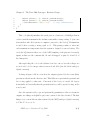
The following is a simpe Arduino code to read the three outputs from the accelerometer and print the values via the serial port [18].
1
2
3
4
5
6
7
8
9
10
11
12
13
14
15
16
17
18
19
20
21
22
23
/* MMA7631 ANALOG 3 axis accelerometer test */
char breaktrans ;
float valx , valy , valz ;
void setup ()
{
while (! Serial ) ;
Serial . begin (19200) ;
Serial . println ( " Send a 1 to start transmission ) " ) ;
while ( Serial . available () <= 0) {}
// waiting for some
string ..
breaktrans = ’1 ’;
// to start the
test
}
void loop ()
{
breaktrans = Serial . read () ;
if ( breaktrans == ’1 ’) {
// read data from sensor
while (1) {
breaktrans = Serial . read () ;
// to be able to stop
valx = analogRead ( A0 ) ;
valy = analogRead ( A1 ) ;
valz = analogRead ( A2 ) ;
Serial . print ( " x " ) ; Serial . println ( valx ) ;
23
Chapter 2. The Pivot Shift Prototype: Hardware Design
24
Serial . print ( " y " ) ; Serial . println ( valy ) ;
27
Serial . print ( " z " ) ; Serial . println ( valz ) ;
28
if ( breaktrans == ’0 ’) { break ;}
// stop transmission
29
}
30
}
31 }
This code (sketch) initializes the serial port at a baud rate of 19200bps then in
order to start the transmission the Arduino waits until receiving a string ’1’ (can come
from another embedded system or computer connected to the device). Transmission
is ended after receiving a string equal to ’0’. This pairing routine to start and
end transmission is important when the system is designed to run on battery. The
analogRead() function takes care of the ADC sampling of the pins used as analog
inputs, in this case the constants A0, A1 and A2 mapped to pins 23, 24 and 25 of
the Atmega328.
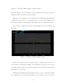
After uploading the code to the Arduino board we can see how the voltages are
received and coded to integer values between 0 and 1023 (due the 10 bit analog to
digital converter).
Looking at figure 2.14b it’s clear how the output registered by the z axis (blue)
presents an offset from the other two axis. This difference represents the gravitational
force being applied to that axis. Conversely if the device is rotated 90 degrees
horizontally and vertically then the gravitational force will be spotted acting on the
x and y axis.
Once the system is able to get and perform the quantization of the accelerometer
outputs, two things are helpful to give some context to the data obtained. The first
thing to is to convert the raw value returned by the ADC (analog to digital converter)
to Volts. To do so we do:
ADCV oltage = RawADC ∗ V ref /1023
24
(2.2)
Chapter 2. The Pivot Shift Prototype: Hardware Design
(b) Output for x, y and z axis
(a) Arduino IDE serial port monitor
Figure 2.10: Reading the output of the MMA7361LC accelerometer resting at horizontal position
Where RawADC is the integer from 0 to 1023 got from the ADC, V ref is the reference
voltage in this case 3.3V and the 1023 representing the levels of quantification or
discrete values the ADC can provide.
After this, the Zero-g voltage is subtracted from the ADCV oltage . The Zerog voltage is the voltage that each of the axis outputs when no acceleration (0g
acceleration) is being applied. This is typically provided in the device data-sheet
although is easy (and recommended) to calculate practically because can vary from
chip to chip.
Xout
Yout
Zout
Data-Sheet
1.65 V
1.65 V
2.45 V
From
1.591
1.705
2.205
device testing
V
V
V
Table 2.1: Zero-g voltage taken from data-sheet and device testing
25
Chapter 2. The Pivot Shift Prototype: Hardware Design
(a) Gravity acting on Y axis
(b) Gravity acting on X axis
Figure 2.11: The effect of gravity on accelerometer readings
From the table above it can be seen a slight difference between the typical values
provided from the data-sheet and the actual values got from testing the device.
Now finally to go from Volts to G’s (1g = 9.8m/s2 ) the following calculation is
performed for each of the axis
Gx = (ADCXV oltage − ZeroX )/sensitivity
Gy = (ADCY V oltage − ZeroY )/sensitivity
(2.3)
Gz = (ADCZV oltage − ZeroZ )/sensitivity
where ZeroX , ZeroY , and ZeroZ are 1.59V, 1.705V and 2.205V respectively (from
table 2.1). The sensitivity value comes directly from the device specifications which
can be 800mv/g or 206 mv/g for ±1.5g and ±6g operation ranges, which in this case
is set to operate at ±1.5g.
26
Chapter 2. The Pivot Shift Prototype: Hardware Design
2.2.4
LSM9DS0: 3D Accelerometer/Gyroscope module
The LSM9DS0 is a system in package featuring a three-axis accelerometer, gyroscope
and magnetometer also known as a nine degrees of freedom device (9DOF). Each
of the three sensors in the device supports programmable operating ranges. The
accelerometer has a full scale of ±2g/±4g/±8g/±16 g, the gyroscope an angular rate
of ±245/ ± 500/ ± 2000 dps (degrees per second) and the magnetometer a magnetic
field of ±2/ ± 4/ ± 8/ ± 12 gauss. The device includes an I2 C serial bus supporting
standard and fast mode (100 kHz and 400 kHz) and an SPI serial interface.
Accelerometer and Gryoscope characteristics are found in the following tables:
Parameter
Test conditions
Linear acceleration
measurement range
Linear acceleration
sensitivity
Linear acceleration sensitivity change vs. temperature
Linear acceleration typical
zero-g level offset accuracy
Operating
temperature
range
Linear acceleration=±2
Linear acceleration=±4
Linear acceleration=±6
Linear acceleration=±8
Linear acceleration=±16
From -40 ◦ C to +85 ◦ C
Specification
±2
±4
±6
±8
±16
0.061
0.122
0.183
0.244
0.732
±1.5
Unit
±60
mg
−40 to +85
◦
g
mg/LSB
%
C
Table 2.2: LSM9DS0 Accelerometer characteristics
Before continuing, lets define some of the terminology showed on the previous
tables. When talking about sensors it is common to see terms like range, sensitivity
and zero levels.
27
Chapter 2. The Pivot Shift Prototype: Hardware Design
Parameter
Test conditions
Angular rate=±245
Angular rate=±500
Angular rate=±2000
From -40 ◦ C to +85 ◦ C
Specification
±245
±500
±2000
8.75
17.50
70
±2
245 dps
500 dps
500 dps
±10
±15
±25
Angular rate
measurement range
Angular rate
sensitivity
Angular rate sensitivity
change vs. temperature
Angular rate typical
zero-rate level
Unit
dps
mdps/digit
%
dps
Table 2.3: LSM9DS0 Gyroscope characteristics
The range represents the levels the sensor’s output signal can achieve (maximum
and minimum values), that in regards of the accelerometer is expressed in ±g, with
option of five different ranges to choose from. For instance, if the accelerometer is
working in the ±2g range, this means that if a 4g force is applied it will not be
properly displayed by the output since the maximum is set to 2g. For this reason is
important to know the application in which the device will be used on, to select the
appropriate output range. From the previous statement would be very tempting to
say that the best solution is to select the broadest range, however this is were the
sensitivity comes into play.
The sensitivity is the ratio of change between the input and output signal in
the sensor. The metric is specified at a particular operating voltage typically in
mV/unit for analog devices and LSB/unit or unit/LSB for digital output devices.
For the accelerometer it’s seen in mg/LSB, where LSB stands for least significant bit.
LSB relates to accuracy of the digital representation of the measured unit, in this
case acceleration. For example from table 2.2 we see that when using range ±2g there
is a sensitivity equal to 0.061mg/LSB, this means that when the lowest order bit in
the output changes, the acceleration had a change of 0.061mg’s or 0.0005978m/s2 ,
28
Chapter 2. The Pivot Shift Prototype: Hardware Design
in other words 0.0005978m/s2 is the tinniest change in acceleration the sensor can
have between readings. Looking at the specification can be seen how for a broader
range the sensitivity value increments as well, which makes the sensor less accurate.
Additional to the convenience of providing both acceleration and gyroscope metrics in the same chip, the LSM9DS0 output signals deliver digital data in useful
units like G’s and dps for acceleration and angular velocity respectively. That being
said, when interfacing with digital sensors like the LSM9DS0 there is no longer need
of using the analog to digital converter of the Arduino board, removing some overhead of reading and sampling the analog inputs, as well as making the conversion
of ADC units to Voltage and then G’s as seen previously using the MMA7361LC
accelerometer.
Other fact worth mention is that the digital sensor eases the scalability of the
system, e.g when using the MMA7361 three input lines are required to communicate
the device with the Arduino. Now, if we were to implement a second accelerometer or gyroscope in the system, three additional lines would be required (Xout , Yout ,
Zout ), which equals the maximum number of analog inputs for the Atmega328 microcontroller that supports up to 6 (without multiplexing[19]). In the other hand, to
communicate two LSM9DS0’s with the Arduino (2 accelerometers and 2 gyroscopes)
via I 2 C requires only two lines as the following section will show.
2.2.5
I2 C Protocol
From the two protocols offered by the LSM9DS0 I2 C was the one used to communicate the accelerometer to the Arduino board.
The I2 C protocol requires two wires to connect a single master to a slave, unlike
SPI that requires four lines to achieve the same. I2 C supports multi-master system
that allows more than one master to communicate with all slaves in the bus. I2 C
29
Chapter 2. The Pivot Shift Prototype: Hardware Design
Term
Transmitter
Receiver
Master
Slave
Description
The device which sends data to the bus
The device which receives data from the bus
The device that initiates a transfer, generates clock signals and terminates transfers
Device addressed by the master
Table 2.4: I2 C terminology
supports two main data rates called normal and fast mode running at 100kHz and
400 kHz respectively.
There are two signals associated with the I2 C bus: the serial clock line (SCL)
and serial data line (SDA). The SDA line is a bidirectional line that can be used for
sending and receiving data both by master and slave devices. These lines use pull-up
resistors to keep a high state when the bus is free.
The bus drivers are “open drain”, which means that they can pull the signal line
to a low state, but cannot turn it to high. This implementation prevents potential
damage to the drivers and excessive power dissipation, disables what is known as
bus contention where a device tries to drive the line high while other tries to pull it
low.
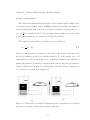
Bus operation
The operation on the bus starts when the master performs a start condition, which
is defined as a high to low transition on SDA (data line) while SCL (clock line) is
high, at this point the bus is considered busy. The next byte of data contains the
address of the slave in the first 7 bits, the 8th bit determines whether the device is
transmitting or receiving from the slave, while a 9th bit is used as NACK/ACK bit.
When this address is sent, then all devices compare it with their own to check if they
30
Chapter 2. The Pivot Shift Prototype: Hardware Design
are being addressed by the master.
Acknowledge is mandatory for this protocol, both for the data and address frames.
Once the first 8 bits (address and r/w) are sent, the receiving device is given control
over the SDA line. To successfully generate the acknowledge, the receiver needs to
pull low the SDA line prior the 9th clock pulse.
Figure 2.12: I2 C signals, showing the start condition, address and data frames, ,and
stop condition
Data transmission can start after the address frame has been sent. During data
transmission the master continues the with the control and generation of the clock
pulses while the data is placed in SDA line by the master or the slave, depending the
value of the r/w bit (8th bit of address frame). The number of data frames is arbitrary, and most slaves will auto-increment the internal registers to allow subsequent
reads or writes.
The operation of the protocol end with a stop condition defined by a low to high
transition on the data line SDA while the clock line stays high.
2.2.6
Getting data from the LSM9DS0
This section shows the required connections to be made between the LSM9DS0
and the Arduino board in order to communicate. The following schematic shows
a configuration of two LSM9DS0 connected to the Arduino Mini board using the
31
Chapter 2. The Pivot Shift Prototype: Hardware Design
previously introduced I2 C communication protocol.
Figure 2.13: Schematic diagram of two LSM9DS0’s connected to an Arduino Mini
board under I2 C
Compared to the connection of the MMA7361 back in figure 2.9 this one looks
pretty straightforward considering that includes two LSM9DS0 modules. In this
configuration the Arduino acts as master for the I2 C leaving the LSM9DS0’s as
slaves.
The two LSM9DS0 boards share the bus for the clock and data signals SCL and
SDA. The clock signal is controlled and generated by the Arduino while the SDA can
be used to send and receive data from the accelerometers. Initially both LSM9DS0
boards have the same address which makes impossible to the master to differentiate
from each other. To solve this, the least significant bit of the address of one of the
modules is changed by setting pins SDOG and SDOXM to a low state. Arduino
board and inertial modules are powered up by 3.3 Volts.
32
Chapter 2. The Pivot Shift Prototype: Hardware Design
The next code snippet shows the Arduino data adquisition from the LSM9DS0
inertial module.
1
2
3
4
5
6
7
8
9
10
11
12
13
14
15
16
17
18
19
20
21
22
23
24
25
26
27
28
29
# include < Wire .h >
# include < Adafruit_LSM9DS0 .h >
# include < Adafruit_Sensor .h >
/*
* i2c arduino pins
* Arduino analog input 5 - I2C SCL
* Arduino analog input 4 - I2C SDA
*/
Adafruit_LSM9DS0 lsm = Adafruit_LSM9DS0 () ;
char breaktrans ;
void setupSensor ()
{
// 1.) Set the accelerometer range
lsm . setupAccel ( lsm . L S M 9 D S 0 _ A C C E L R A N G E _ 2 G ) ;
// 2.) Setup the gyroscope
lsm . setupGyro ( lsm . L S M 9 D S 0 _ G Y R O S C A L E _ 2 4 5 D P S ) ;
}
void setup ()
{
while (! Serial ) ;
Serial . begin (19200) ;
Serial . println ( " Send a 1 to start the test " ) ;
while ( Serial . available () <= 0) {}
// waiting for some
string ..
breaktrans = ’1 ’;
// to start the
test
// Try to initialise the device
if (! lsm . begin () )
{
Serial . println ( " Unable to initialize the LSM9DS0 . Check
your wiring ! " ) ;
while (1) ;
}
Serial . println ( " Found LSM9DS0 9 DOF " ) ;
Serial . println ( " " ) ;
}
30
31
32
33
34
35
36 void loop ()
37 {
33
Chapter 2. The Pivot Shift Prototype: Hardware Design
38
41
42
43
44
45
46
47
48
49
50
51
52
53
54
55
56
57
58 }
breaktrans = Serial . read () ;
if ( breaktrans == ’1 ’) {
// read data from sensor
while (1) {
breaktrans = Serial . read () ;
// continue to read to catch
stop condition
// getting the sensor event
sensors_event_t accel , mag , gyro , temp ;
// from
adafruit sensor master library
lsm . getEvent (& accel , & mag , & gyro , & temp )
// reading the accelerometer
Serial . print ( " accelx " ) ; Serial . println ( accel .
acceleration . x ) ;
Serial . print ( " accely " ) ; Serial . println ( accel .
acceleration . y ) ;
Serial . print ( " accelz " ) ; Serial . println ( accel .
acceleration . z ) ;
// reading the gyroscope
Serial . print ( " gyrox " ) ; Serial . println ( gyro . gyro . x ) ;
Serial . print ( " gyroy " ) ; Serial . println ( gyro . gyro . y ) ;
Serial . print ( " gyroz " ) ; Serial . println ( gyro . gyro . z ) ;
if ( breaktrans == ’0 ’) { break ;}
// stop transmission
}
}
This code provides the same functionality shown in the program for the MMA7361
with the difference of addition of angular velocity provided by the gyroscope. Two
main libraries are imported, Wire which allows communication with I2 C/TWI devices, and the Adafruit library[20] that incorporates the class Adafruit LSM9DS0
that includes useful functions to easily configure the device to the different ranges as
well to get the outputs from each of the axis and sensors available (accelerometer,
gyroscope and magnetometer) without coding to a register level.
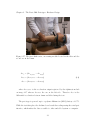
The function setupAccel lets you choose the range of operation for the accelerometer from the following options
• LSM9DS0 ACCELRANGE 2G
34
Chapter 2. The Pivot Shift Prototype: Hardware Design
• LSM9DS0 ACCELRANGE 4G
• LSM9DS0 ACCELRANGE 8G
• LSM9DS0 ACCELRANGE 16G
whereas setupGyro allows setting the angular velocity range to
• LSM9DS0 GYROSCALE 245DPS
• LSM9DS0 GYROSCALE 500DPS
• LSM9DS0 GYROSCALE 2000DPS
sensor event t is a structure that provides a single sensor events in a common format.
In this way each sensor creates its own object from which it can retrieve its respective
data from. Calling getEvent grabs sensors new data, so in order to continuously get
new readings it needs to be executed recursively.
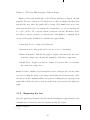
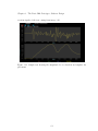
Similarly to the test done with the analog accelerometer, these are the results of
flashing the Arduino board with the previous code and getting some data from the
sensor.
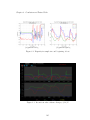
As expected the graph of the three axis acceleration at rest (horizontal postition)
is pretty similar of what was presented on 2.14b with the difference that in this case
the outputs are in g’s already.
With the goal of comparing the sampling rate between each of the chips, previous
Arduino programs were slightly modified to transmit data during a period of 10
seconds. In the results the MMA7361C delivered an average of 165 triplets (Xout,
Yout, Zout) as the LSM9DS0 delivered an average of 650 triplets. This difference
is caused in some proportion to the overhead caused by reading the analog inputs
and performing the analog to digital conversion when using analog sensors. When
35
Chapter 2. The Pivot Shift Prototype: Hardware Design
(b) Output for x, y and z axis
(a) Arduino IDE serial port monitor
Figure 2.14: Reading the output of the LSM9DS0 accelerometer resting at horizontal
position
performing the same test but adding the angular velocity readings from the gyro the
results were an average of 290 samples for each variable.
2.3
The Prototype
This section describes the idea behind the pivot shift tester prototype and how it
was implemented. Going back to what was introduced in the first chapter we saw
the different medical tests and tools commonly used in the diagnose of the injury of
the anterior posterior ligament. We were able to identify them in two main groups:
• imaging techniques
• routine tests
The problem with the first group (imaging) resides in the fact that uses equipment
considerably expensive, in such a way that the patient often needs to visit a clinic or
36
Chapter 2. The Pivot Shift Prototype: Hardware Design
hospital to take test. It is highly unlikely to find them in the specialist’s office and
both CT scans and MRI typically have a cost superior to $1000 US dollars. Aside
from the economic factor, other disadvantage that the imaging techniques have is
that both tests the patient’s leg and knee in a static environment, reason why in
some cases is difficult to assess a definitive diagnose if the information provided by
the image is not completely evident.
Here we provide an example, the first image (MRI) shows a complete tear of the
ACL ligament. In an image like this the specialist is able to confirm the ACL injury
without much hesitation, because the ligament simply is not there anymore.
Figure 2.15: MRI, complete tear of ACL ligament
Compared to the first image this second one looks not that straightforward. The
MRI shows an incomplete tear of the ACL ligament, that still represents a problem,
however is difficult to grade the severity of the damage by the image itself.
Is in this situation where routine tests like the lachman and pivot shift test help
the specialist providing information about the stability of the knee in motion. From
what was shown in chapter 1, it can be established that the results of the lachman test
can be related to the results of the test using the KT-1000 arthrometer[5]. Therefore
can be stated that the KT-1000 helps to provide quantitative (anterior posterior
37
Chapter 2. The Pivot Shift Prototype: Hardware Design
Figure 2.16: MRI, partial tear of ACL ligament
translation in millimeters) information to the lachman test.
Unlike the lachman test, at this point there is not a definitive instrument or tool
used for the measurement of the pivot shift. The work shown in this thesis project
tries to fill that gap by introducing a non-invasive prototype aimed to be used during
the pivot shift maneuver to collect data about the test.
Recalling image 1.7, it is known that what makes particular this test is the application of valgus and rotational forces, which will be tracked using accelerometer
and gyroscopes modules.
The concept is to implement two sensing modules, one placed in the patient’s
tibia and the other in the bottom of the femur. With this it is possible to take one
point as reference and get differential acceleration readings representing the anterior
posterior translation force applied during the test.
Both acceleration modules are connected to the Arduino board, which handles
the data acquisition and performs the following calculation for each new sample:
38
Chapter 2. The Pivot Shift Prototype: Hardware Design
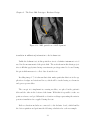
Figure 2.17: The pivot shift tester, one sensing module located in the tibia and the
second one in the femur
Accx = (AccXf emur − AccXtibia )
(2.4)
Accy = (AccY f emur − AccY tibia )
Accz = (AccZf emur − AccZtibia )
where AccXf emur is the acceleration output registered by the rightmost module
on image 2.17 whereas AccXtibia the one on the left side. Therefore Accx is the
differential acceleration between femur and tibia during the test.
The prototype is powered up to a polymer lithium ion (LiPO) battery of 3.7V.
While the test takes place the Arduino board sends the readings using the serial port
interface, which makes the data accessible to other embedded system or computer.
39
Chapter 2. The Pivot Shift Prototype: Hardware Design
The next chapter describes in detail how the data is presented to the user in
real time (while the test happens) via an user interface created in the Processing
programming language.
40
Chapter 3
The Pivot Shift Prototype:
Software Design
In this chapter we explore the design and implementation of the software created
to interact with the pivot shift prototype previously introduced. The application
visually displays the readings from both the accelerometers and gyroscopes while the
test takes place. The application was coded in the java based programming language
Processing.
3.1
Processing
Processing is an open source, cross-platform programming language and integrated
development environment initiated back in 2001 by Casey Reas and Benjamin Fry
from the MIT Media Lab.
Initially intended as a introduction to programming for visual artists and designers, now has evolved to a development tool for professionals being used by students,
41
Chapter 3. The Pivot Shift Prototype: Software Design
researchers and hobbyists alike.
Processing takes software concepts and transforms it to principles of visual form,
motion and interaction. Within this visual context, Processing is set to work as
a software sketchbook. The language is text based and implements a wide variety
of functions and libraries aimed for computer graphics techniques like vector/raster
drawing, color models, image processing, network communication, and object oriented programming. Custom made libraries can extend the functionality to generate
sounds, send and receive data in different formats and enhance 2D and 3D file formats.
All programs created on Processing are a subclass of the PApplet Java class,
additional classes are treated as inner classes when the code is translated to Java
code before compilation.
Processing allows two main modes, the Java and Javascript mode, applications
in Java are executed as a standalone window applet whereas the Javascript mode
translates the code to work and run in a browser. Applications can be exported to
Linux, Mac and Windows operating systems, with the option to embed Java runtime
which is recommended to ensure the same performance between platforms.
Core libraries, and code used in the exported application and applets are licensed
under GNU Lesser General Public License, allowing the programmer to release their
code with license of choice[21].
There is extensive community support and resources to learn this programming
language, recommended sites for this purpose are https://processing.org and
http://www.openprocessing.org.
42
Chapter 3. The Pivot Shift Prototype: Software Design
3.2
The Basics
Here we describe the particularities of the programs created in this programming
language and a basic example, which will help to assimilate more easily the main
application to be introduced later on [22].
In Processing, all sketches have two main functions:
• setup()
• draw()
The setup() function is called once during the execution of the sketch and it is
used to initialize variables and run setup routines. The draw() function is the main
loop of the application, and it runs automatically after setup() function, it should
not be called explicitly. The function executes the lines of code contained inside its
block until the application stops or noLoop() is called. The functions used to control
the behavior of the main loop are:
• noLoop()
• redraw()
• loop()
If the main loop is stopped by noLoop() it can be reestablished using loop() or in
the other hand if redraw() is called then the code inside draw() will be re-executed
only one more time.
The following code snippet is an equivalent of a hello world for processing. This
sketch will paint a point in the current position of the mouse cursor.
43
Chapter 3. The Pivot Shift Prototype: Software Design
1
2
3
6
7
8
9
10
11
12
13
14
15
16
// Hello world
void setup () {
size (400 , 400) ;
stroke (200 ,22 ,22) ;
strokeWeight (5) ;
background (200 , 200 , 200) ;
fill (240 ,20 ,20) ;
textSize (25) ;
text ( " Hello World " ,50 ,50) ;
}
void draw () {
point ( mouseX , mouseY ) ;
}
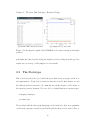
These is the result
Figure 3.1: Simple application using Processing
Now that we showed the premise of programming in processing can go further
and talk about the design of the pivot shift user interface software.
44
Chapter 3. The Pivot Shift Prototype: Software Design
3.3
The Pivot Shift Software
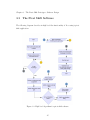
The following diagram describes in high level the functionality of Processing’s pivot
shift application.
Figure 3.2: High level algorithm for pivot shift software
45
Chapter 3. The Pivot Shift Prototype: Software Design
All starts establishing the communication with the embedded device, this is done
via serial port. When using the Arduino board there are two options from which the
serial port can be accessed, the first one via the digital pins 0 (RX) and 1 (TX), and
the second one and the used in this project via USB. First there is a routine to check
for the presence of a device connected in the serial port. After the device is found,
then a pairing routine is executed. This routine establishes the the mode of operation
for the test which consist of whether the user wants to use both sensing modules (to
calculate differential metrics), or work with only one accelerometer. Once operation
mode is defined a message is sent back to the embedded device to properly setup
and initialize the sensors. Concluded the setup, the Arduino sends back a string
specifying that is ready to start the test, at this point is in control of the Processing
application to start the data acquisition.
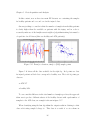
The user begins the test via the user interface and starts to poll data from the
sensors. While the test runs the acquired data is showed both in text format and by
plotting a graph. Finally when the user stops the test an csv file containing all the
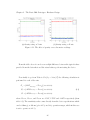
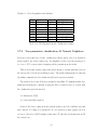
readings from the test is saved along with a png image of the graph.
3.3.1
The Coding
Before starting coding the application few libraries are imported:
• processing.serial
• controlP5[23]
• java.io
processing.serial enables support for the serial port class, controlP5 is GUI and
controller library that incorporates elements like sliders, buttons, toggles, knobs,
46
Chapter 3. The Pivot Shift Prototype: Software Design
textfields among others to ease user interaction. This library is very convenient
because Processing don’t provide GUI elements out of the box although they can be
manually implemented. The java.io library is used to manage filesystem capabilities
and have access to local files and be able to save test results to disk.
Figure 3.3: A selection of controllers available with ControlP5 library
As was mentioned previously, the core structure of a Processing sketch is found
in the functions setup() and draw(). Global variables are allowed as well, and they
need to be declared outside the scope of setup() and draw() functions. Many global
variables and classes are defined to setup the visual environment among other things
including:
• initialize serial port class
• initialize ControlP5 class
• setup window size and color scheme
• define text labels and plotting area position and defaults
47
Chapter 3. The Pivot Shift Prototype: Software Design
• setting default operation mode:
– 1 accelerometer
– 2 accelerometers
• plot mode:
– acceleration only
– accelerometer and gyroscope
• declare acceleration and rotation arrays
After global variables and classes are defined setup() is called and draws the initial
user interface positioning text labels, plotting area and GUI elements like buttons
and toggles, as well as looking for a connected device in the serial port. At the end
of setup() execution we end up with this:
Figure 3.4: User interface for the pivot shift tester
48
Chapter 3. The Pivot Shift Prototype: Software Design
Figure 3.4 shows the initial state of the UI (user interface) at launch. At that
point the UI can be defined in 5 blocks showed as yellow rectangles, the first block
indicates the area where the graph will be drawn, block number two is the area
where text labels are placed to indicate the current metric e.g. for acceleration can
be “x 1.25 , y 2.00, z .98” to specify current g values in each axis. Block three is the
area where y axis (acceleration or rotation) and x axis (number of samples) labels
are set for the graph. Fourth block contains four toggle buttons:
• Start-Stop. Used to begin and end the test
• Operation mode. Sets up the test to use one or two accelerometers.
• Enable Magnitude. Switches the graph to display each axis as its own curve
or enables a single curve showing the magnitude of the three components.
• Graph Mode. Toggles view mode to display acceleration only or acceleration
and rotation in a single view.
finally block five contains a dropdown menu to select serial port (in case more than
one device is using the port), a Save image button that saves both an image of the
test and an csv file containing all the data generated during the test. Open previous
graph button allows the user to open an csv file from a previous test and display its
graph.
3.3.2
Beginning the test
Once the application is launched and the visual environment is setup, then the serial
communication between the embedded system and the PC begins.
1 Serial myPort ;
2 try {
49
Chapter 3. The Pivot Shift Prototype: Software Design
3
4
7
8
9
10
myPort = new Serial ( this , portName , 19200) ;
myPort . bufferUntil ( ’\ n ’) ;
println ( " Starting test " ) ;}
catch ( Exception e ) {
println ( " No serial port available " ) ;
}
This sample code initializes the serial port using a baud rate of 19200 bps. The
variable portName holds the name of the serial port selected from the dropdown
menu located in the upper left part of the UI. At this point the embedded system
waits to receive some initialization strings from the serial port indicating how many
accelerometers to use and when to start sending sensor data.
1
2
3
4
5
6
7
8
9
10
11
12
13
14
15
16
17
18
19
20
21
22
23
24 }
if ( theEvent . controller () . name () == " start " ) // Start the test
{
if ( start == true )
{
timestart = millis () ;
if ( first_time == true )
{
println ( " Selected serial port " + dropDownItemName ) ;
portName = dropDownItemName ;
myPort = new Serial ( this , portName , 19200) ;
}
Cleargraph () ;
// clear data arrays to start new
test
first_time = false ;
myPort . bufferUntil ( ’\ n ’) ;
if ( opMode == true ) {
// opMode - Operation mode
myPort . write ( ’b ’) ;
// 2 accelerometers mode
myPort . write ( ’1 ’) ;
}
else {
myPort . write ( ’a ’) ;
// 1 accelerometer mode
myPort . write ( ’1 ’) ;
}
}
50
Chapter 3. The Pivot Shift Prototype: Software Design
This code is executed when the event on the Start toggle is activated (when
pressed), it checks the state of the other toggle called OpMode (right next to Start
toggle) to see if the user chose one accelerometer or two. A boolean value true for
OpMode means using two accelerometers, as false specifies to use only one. Now
the embedded system expects two strings, the first one indicates the mode ’a’ for 1
accelerometer and ’b’ for two, and a start/stop flag used to begin or finalize the test,
’1’ starts as ’0’ terminates.
3.3.3
During the test
Once the embedded system starts sending data from the sensing modules the importance resides in properly display it and store it for future analysis.
The strings the Arduino sends including the sensor’s readings have an specific
format illustrated by the following examples, for acceleration these are valid strings:
• x 1.26
• y 0.98
• z -1.08
and for rotation:
• gx 25.30
• gy 15.00
• gz 85.96
where x, y, and z represent acceleration and gx, gy, and gz rotational metrics from
the gyroscope. Therefore the string is formatted in a ’metric+space+value’ manner.
51
Chapter 3. The Pivot Shift Prototype: Software Design
The strings are parsed during the serial port event in the application, dividing them
in two sections, the first identifying the metric and axis that belongs to, and the last
part is converted to a float specifying the magnitude.
1 if ( sdata . indexOf ( " x " ) >=0) // x axis
2
{
3
sdata2 = split ( sdata , ’ ’) ;
4
arrayx . add ( float ( sdata2 [1]) ) ;
5
}
In this snippet sdata is the string containing the newest line of data from the serial
port. The string then is separated into numerical and metric part.
Six global arrays are defined arrayx, arrayy, arrayz, arraygx, arraygy, arraygz
each one storing the data for its corresponding metric and axis. This is how the
application continuously stores the data coming from the embedded device, the next
step once each of the metrics has at least one sample is to proceed with the display
of the graph.
An additional array arraytime is used. This array keeps track of the minimum
total of samples that all of the metrics have at a given point. The main reason
for this is to know up to what number of sample the graph can be displayed. The
following output displays the number of samples that each array haves at 4 seconds
of elapsed time.
1 x :142 y :142 z :142 gx :142 gy :141 gz :142
:4.291 s
## elapsed test time
For this example arraytime should have a value of 141.
As was showed, the plotting area is defined to use the majority of the UI space.
In Processing the size of the application window is specified explicitly in most cases
using pixels. In other approach it can be set to have a size based on the screen
resolution, which makes the application not to depend on specific hardware. In this
52
Chapter 3. The Pivot Shift Prototype: Software Design
application it is set to have a size of about 85% of the screen width and height. Then
after size is defined two variables are automatically set width and height as we can
see in the code:
1
2
3
4
5
6
7
8
9
10
11
size ( round ( displayWidth *.85) , round ( displayHeight *.85) ) ;
// Single graph layout
plotX1 = 120;
plotX2 = width - 120;
plotY1 = 100; // 70
plotY2 = height - 85;
// Dual layout
plotY1_1 = plotY1 ;
plotY2_1 = plotY1 + plotY2 *.40; // end of first plot area
plotY1_2 = plotY2_1 +50; // start of second area for plot
plotY2_2 = plotY1_2 + plotY2 *.40; // end of second plot area
the size() function takes two parameters being the width and height. What the
code does is setting variables that represent corners of the rectangle enclosing the
plotting area. As the application is set to show acceleration or acceleration and
rotation, two layouts are predefined. This code is found inside the setup function
called at the beginning of the sketch and having those dimensions already defined
facilitates switching layout during runtime. The next screen-shot illustrates the
position of the rectangle’s vertices for the plotting areas. Function rect(a, b, c, d) is
used to draw the rectangles each parameter describing:
• a- x-coordinate of rectangle (upper left corner by default)
• b- y-coordinate of rectangle
• c- width of the rectangle
• d- height of the rectangle
Therefore, in order to draw rectangles for acceleration and rotation rect() needs
to be called with parameters:
53
Chapter 3. The Pivot Shift Prototype: Software Design
1
4
rect ( plotX1 , plotY1_1 , plotX2 , plotY2_1 ) ; // upper rectangle
acceleration
rect ( plotX1 , plotY1_2 , plotX2 , plotY2_2 ) ; // bottom , rotation
Figure 3.5: Pivot Shift UI, dual layout presentation
Now that the area to display the graphs is properly defined, it is time to map the
values obtained from the sensors (acceleration and rotation) into the area enclosed
by the rectangles.
The final graph for each of the metrics has as the Y axis the values for acceleration
and rotation, as the X axis represents the number of samples for the test. To draw
this line graph, sample i is connected with sample i + 1 by a line. To achieve this
the first thing is to transform the value of the sample (acceleration or rotation value)
to its corresponding pixel value inside the coordinate system created by the plotting
rectangle.
This is done using the map() function:
54
Chapter 3. The Pivot Shift Prototype: Software Design
3
4
5
float map ( float value , float low1 , float high1 ,
float low2 , float high2 ) {
return high2 + ( high2 - low2 ) *(( value - low1 ) /( high1 low1 ) )
6 }
where value stands for the number to map or transform, low1 and high1 are the
minimum and maximum values in the original space, in this case, if the metric is
acceleration then low1 should be the minimum value of all the acceleration samples
stored so far, as high1 works in the same way taking the maximum. The arguments
low2 and high2 represent the new range in which the value will be mapped into. In
short, the function takes a numeric value and transforms it from the scale low1−high1
to a new value in the range from low2 − high2.
For example, if the current value for acceleration is 1.25 g’s, then map function
has to be called twice to get the corresponding X and Y position (in pixels) of the
sample inside the plotting area.
1
2
xplot = map (1.25 ,1 , arraytime . size () , plotx1 , plotx2 ) // X
position in pixels
yplot = map (1.25 , minval , maxval , ploty2 , ploty1 )
// Y position
in pixels
For the X axis the original boundaries are between 1 (the minimum number of
samples) and the total number of samples. The new range is defined by the width
of the plotting area that is between plotx1 − plotx2. The Y axis goes from the range
defined by the minimum and maximum acceleration values to the range between the
points ploty2 − ploty1.
To finally reproduce the graph of the three axes in real time , a function called
P lotarray(arraytime, arraymetric, strokecolor) is defined. The first argument arraytime is the array holding the values for the horizontal axis, arraymetric can be
one of six choices arrayx, arrayy, arrayz, arraygx, arraygy, or arraygz storing the
55
Chapter 3. The Pivot Shift Prototype: Software Design
acceleration or rotation of one of the axes. The strokecolor parameter specifies the
color of the line to be drawn. Therefore, in order to generate the continuous graph
of the acceleration metric, the following piece of code needs to be called inside the
draw() loop:
1
2
3
PlotArray ( arraytime , arrayx , " R " ) ;
PlotArray ( arraytime , arrayy , " G " ) ;
PlotArray ( arraytime , arrayz , " B " ) ;
leading to a graph like this:
Figure 3.6: Sample acceleration graph: x axis in red, y axis green, and z axis in blue
since the P lotarray() function is called during the main loop, it automatically
scales the graph to the values stored in the data arrays. The image shows the
resulting acceleration (in g’s) signals for each of the axes during the test.
3.3.4
From angular velocity to angular displacement
Recalling the features of the sensing module LSM9DS0 from the previous chapter,
we know that incorporates both an accelerometer and a gyroscope. The acceleration
is presented as g’s while the angular velocity is presented in dps (degrees per second). Angular velocity is defined as the rate of change in angular displacement while
56
Chapter 3. The Pivot Shift Prototype: Software Design
angular displacement is the angle through which a body is rotated in a specific sense
(direction) and axis. This section shows the procedure taken to convert gyroscope
output from angular velocity to angular displacement.
Directions for acceleration and angular rate are presented in the following image:
Figure 3.7: LSM9DS0 module: directions for acceleration and angular rates
the directions for rotation of each of the axes are presented, which are commonly
known in flight dynamics like:
• roll: rotation in X axis
• pitch: rotation in Y axis
• yaw: rotation in Z axis
For this the Pivot Shift application it was considered to be more helpful to consider the angular displacement rather than the angular velocity. Using angular dis-
57
Chapter 3. The Pivot Shift Prototype: Software Design
placement allows to clearly identify the directions which the prototype was rotated
during test time, as it will be presented shortly.
Expressed in other terms, as we recall that the Pivot Shift maneuver takes both
a valgus and rotational force, it is assumed that we can track the valgus force via
acceleration while for rotation angular displacement is needed rather than velocity.
Now it will be compared the results of using angular velocity and angular displacement.
Figure 3.8: Sample test using angular velocity
Both of the tests showed by the graphs describe a similar motion as it can be
seen from the acceleration plot (upper one). Initial state of the device is at rest in
horizontal position, then it is rotated in an angle between 20◦ and 30◦ in the X axis
(take figure 3.7 as reference).
Analyzing the first image showing angular velocity, can be seen how the angular
speed picks up at the very moment that the object accelerates on the Y axis, after
58
Chapter 3. The Pivot Shift Prototype: Software Design
Figure 3.9: Sample test using angular displacement
that point starts to lose velocity de-accelerating to return to its initial state. While
this still is useful, it cannot provide information of the magnitude of the rotation,
which is clearly seen in the subsequent image.
Looking at the graph using angular displacement, the movement done during
the test can be reconstructed in some way, it can be said that while the device was
positively rotated (rolled) about 23◦ it reached an acceleration on the Y axis about
0.374 g’s.
The method used to transform the angular velocity to angular displacement involved adding the timestamp of each of the angular velocity samples got from the
embedded device, in this way is known the difference in time between the current sample and the one received previously. To have that information the function millis()
was used, which returns the number of milliseconds since the program started.
To provide the difference in time between samples two variables are used, one
59
Chapter 3. The Pivot Shift Prototype: Software Design
representing sample i (current sample) and sample i − 1 (previous sample). Once
the difference between the samples is known, angular displacement can be described
as:
Angle =
(timestampi − timestampi−1 )
∗ AngularV eli
1000
(3.1)
where both timestamps are provided in milliseconds by the function millis() and
AngularV eli is the current angular rate (dps) provided by the gyroscope, and Angle
represents the angular displacement between sample i and sample i − 1. Next table
shows an example of how angular displacement is calculated in three consecutive
samples. First column represents the timestamp difference between the two samples
in seconds, the second column is the current angular rate coming from the gyroscope
in dps, and the third column shows the resulting angular displacement (degrees)
between consecutive samples.
tgxi − tgxi−1 (s)
0.03
0.03
0.029
Angular Vel. (dps)
-1.71
-2.23
-1.78
Angular displacement (◦ )
-0.0513
-0.0669
-0.05162
Table 3.1: Conversion from angular velocity to angular displacement in X axis
3.3.5
Ending the test and storing data
Once the Pivot Shift maneuver has been performed the test can be terminated, to
do so it’s a matter of sending a string ’0’ to the Arduino executing the following line
of code:
1
myPort . write ( ’0 ’) ;
60
Chapter 3. The Pivot Shift Prototype: Software Design
when the Arduino receives the string stops sending sensing data and stays in an idle
state waiting for the next test to start, sending a string ’1’ enables that.
At this point the user can save the test data on an csv file and a png image, in
this way the graphs can be easily reproduced using an spreadsheet software and the
data can be further analyzed.
Additionally to storing the acceleration and rotation metrics from each of the axes
the software calculates the magnitude of both of the metrics to provide an additional
graph in which the three axes are combined into a single signal, e.g. to calculate
acceleration’s magnitude:
accelerationmag
q
= 2 acceleration2X + acceleration2Y + acceleration2Z
(3.2)
Figure 3.10: Sample test showing axes signals individually
where accelerationX , accelerationY , and accelerationZ are acceleration samples
for each of the axes. Figure 3.11 illustrates the magnitude for the acceleration and
61
Chapter 3. The Pivot Shift Prototype: Software Design
rotation signals of the test coming from image 3.10.
Figure 3.11: Sample test showing the magnitude for acceleration and angular displacement
62
Chapter 4
Clinical Trials
This section explains the origin of the previously collected data set used for the
statistical analysis in this thesis.
Once the hardware and software were implemented, a completely functional prototype based in the first accelerometer MMA7361LC was handed off to a medical
staff leaded by the orthopedist Edmundo Berumen Nafarrete M.D. and Carlos Vega
Najera M.D. from the the Christus Murguerza hospital located in Chihuahua, Mexico
with the goal of testing the prototype in clinical trials.
The inclusion criteria for this trials consisted on patients who attended orthopedic
examination with the specialist and volunteer to be part of the study, no gender, age
or specific medical conditions were restricted to the study.
The study group included a total of 156 patients, with mean age 24; range, 11-76
years; 37 women, 119 men. All patients participated voluntarily in the study by
reading and signing a consent form approved by Christus Murguerza hospital ethics
committee. Clinial trials took place from May 2013 to May 2014.
The study group can be further classified in three groups:
63
Chapter 4. Clinical Trials
• healthy patients.
• patients with previous knee or leg condition unrelated to an ACL injury.
• patients with the ACL (anterior cruciate ligament) injury.
For this trails each patient was submitted to two clinical tests:
• pivot shift test
• KT-1000 test
The examiners group was small consisting of 2 physicians and the lead surgeon.
Physician were instructed by lead surgeon on the execution of the pivot shift technique in order to perform the test as similarly as possible.
The pivot shift shift test was perform three times in each knee for every patient
with the intention of assessing test repeatability. Patients with a previously confirmed ACL diagnosis where submitted to special treatment and had the test done
under anesthesia.
For each of the patients, clinical evaluation of the pivot shift maneuver was determined manually by the physician and documented to keep track on patients with
positive results (to later compare with prototype results). As for the prototype, patient’s results consisted in two images and two csv files corresponding to each leg
acceleration readings.
The KT-1000 test was perform in both of the patient’s legs, documenting the individual result for each one as well as the absolute difference between legs, as described
in chapter 1. This results were manually captured and stored on a spreadsheet file.
Figure 4.2 shows the resulting graph of the acceleration readings coming from the
pivot shift test. The graph shows three noticeable maximum and minimum values
64
Chapter 4. Clinical Trials
for each of the axis. These values are related to each of the three consecutive tests
performed in the patient as described previously.
The specifications of the PC used with the prototype were the following:
1
2
3
4
5
6
7
8
9
10
11
12
13
14
15
16
17
18
19
20
21
22
23
24
## CPU DETAILS # # # # # # # # # # # # # # # # # # # # # # # # # #
Architecture :
i686
CPU op - mode ( s ) :
32 - bit , 64 - bit
Byte Order :
Little Endian
CPU ( s ) :
2
On - line CPU ( s ) list :
0 ,1
Thread ( s ) per core :
1
Core ( s ) per socket :
2
Socket ( s ) :
1
Vendor ID :
GenuineIntel
CPU family :
6
Model :
15
Stepping :
6
CPU MHz :
2000.000
BogoMIPS :
3990.22
Virtualization :
VT - x
L1d cache :
32 K
L1i cache :
32 K
L2 cache :
4096 K
## MEMORY # # # # # # # # # # # # # # # # # # # # # # # # # # # # # # #
total
used
free
Mem :
2014
1610
403
-/+ buffers / cache :
933
1081
Swap :
2044
0
2044
Running Linux distribution:
1
2
3
4
5
6
3.11.0 -12 - generic #19 - Ubuntu SMP Wed Oct 9 16:12:00 UTC 2013
i686 i686 i686 GNU / Linux
Distributor ID : LinuxMint
Description : Linux Mint 16 Petra
Release : 16
Codename : petra
Next chapter introduces the results from testing the prototype on over a hundred
65
Chapter 4. Clinical Trials
patients, performing a data analysis and final thoughts about the results.
Figure 4.1: Prototype used during pivot shift maneuver
Figure 4.2: Graph showing acceleration output per axis from pivot shift test
66
Chapter 5
Data Acquisition and Analysis
This chapter takes the results of testing the pivot shift prototype with a study group
of 156 patients, and analyzes the data files and graphs generated during these trials.
The data generated from the trails consisted in the following:
• 280 csv files
– 140 for left leg
– 140 for right leg
• 280 graphs
– 140 for left leg
– 140 for right leg
• a spreadsheet file containing patient data like: age, weight, KT-1000 test results, and patient observations
The total number of patients during the trials was 156, however inconsistencies
where found in some of them like: missing tests results (csv file) for one of the legs,
67
Chapter 5. Data Acquisition and Analysis
user typos while naming the output file making the test impossible to relate to an
specific patient. Due this complications some of the results had to be excluded in
the following data analysis, leaving a total of 140 patients.
5.1
First glance at graphs and PyPlotter
At the time the data from patients became available, the first thing was to visually
examine the group of graphs in order to get familiar with how real pivot shift tests
acceleration graphs looked like. As well, a particularly interesting thing was to
identify noticeable patterns or differences between the tests coming from left and
right patient’s legs. This is important because as was stated previously, given the
direction of the movement, accelerometers can register both negative and positive
acceleration for any of the given axis.
A Python/Qt[24] application was developed to ease this process of visual examination of the tests, featuring:
• Ability to reproduce graphs from csv files.
• Selectable axis, the user can display acceleration of three axis X, Y, and Z or
choose which ones to use.
• Ability to overlap two graphs: useful to compare left and right legs in a same
patient.
• Graphs can be zoomed and saved to png, svg, and pdf formats.
• Load all csv files from a given directory to easily plot different files.
• Works both for graphs produced by the MMA7361LC prototype (only acceleration) and LSM9DS0 prototype (acceleration + gyro).
68
Chapter 5. Data Acquisition and Analysis
Figure 5.1: Pivot shift plot analyzer
with this, side to side comparison was done in patients to spot if obvious patterns
were present. Next figure shows a patient left and right resulting acceleration graphs.
Figure 5.2: Patient graphs: left leg (left side), right leg (right side)
From this point on, for all upcoming XYZ acceleration graphs the color scheme
used for each axis is:
• X axis: red
• Y axis: green
69
Chapter 5. Data Acquisition and Analysis
• Z axis: blue
Quickly looking at figure 5.2 is difficult to assess something at first glance. The
recreation of the three consecutive pivot shift maneuvers is spotted without much
effort as each of the axis presents 3 peaks or maximum points with similar values.
To compare left leg with right leg accelerations the following plots were done via
the Python application:
(a) X axis
(b) Y axis
(c) Z axis
Figure 5.3: Patient’s side to side acceleration comparison for each axis
These group of plots show the acceleration differences on each of the axis (X, Y,
Z) between left and right leg of the patient. Although one limitation of the data
produced during the trails is noticed, left and right leg tests will not exactly match
in the sense that do not equal in number of samples. This is caused due the fact
70
Chapter 5. Data Acquisition and Analysis
that is practically impossible for the the physician to execute both maneuvers (pivot
shift for right and left leg) with the exact same timing, that is why an offset between
the two tests can be seen as well. Despite this limitation, it will be shown how this
overlapping plots still are useful for the analysis.
After reviewing this new graphs over several patients showing side to side comparison for each of the axis separately one thing became quite noticeable.
Recalling the pivot shift technique, we can consider its two main components as
the rotation and valgus force applied to the knee. This rotation is called internal
tibial rotation which makes reference to the direction in which the movement occurs
and can be described as a rotation towards the direction of the other knee. That
being said, e.g. the internal tibial rotation in the left leg is seen as rotating the leg
towards the right leg.
Now that internal tibial rotation was defined we can go further and state the
following: there should be a noticeable difference between patient’s right and left leg
pivot shift tests, the reason for this is that the rotation applied while performing the
test on each side is opposite to its counter part.
Next graphs make clear this left to right side difference in rotation while the test
takes place.
Figure 5.4 shows side to side acceleration graphs for the X axis on four different
patients. Red curves correspond to left leg while magenta to right. Each of the
graphs shows how right leg values tend to be considerably more positive than left
ones. This effect on the X axis is produced mainly by two factors:
• difference in the direction of the rotation while performing the test on each leg
• the effect to the gravitational force going from the Z axis to the X axis while
rotation happens
71
Chapter 5. Data Acquisition and Analysis
Figure 5.4: Side to side comparison for X axis in four different patients
Next section tries to describe the pivot shift movement and translate it to sections
on the already presented acceleration graphs.
5.2
Interpretation of Graphical Data
This section breaks down portions of the graphs and relates them to parts of the
pivot shift movement to help make sense of the shape found on the data.
The pivot shift maneuver can be divided en the following frames:
1. knee goes into extension
72
Chapter 5. Data Acquisition and Analysis
2. while extension application of tibial internal rotation
3. application of valgus force
4. flexion of the knee while applying both valgus and internal rotation
5. going back to knee joint extension
Figure 5.5 shows each of the movements produced during the pivot shift maneuver
(just listed above). The bottom of the image works as reference to show the initial
position and orientation that the accelerometer has when the test is about to start.
This is critically important because keeps consistency on each axis among the tests.
The way each of the axis is presented (bottom of the image) makes them relate to
particular movements during the maneuver; in this case X axis handles the internal
tibial rotation, Y axis the back and forth movement of the leg, and lastly the Z axis
registers the knee flexion and extension. Due the importance of this, the prototype
was marked to indicate to the physicians the correct way to align the accelerometers
while conducting the tests.
Next to it the graph in figure 5.6 is the resulting left leg plot generated from the
patient test shown in figure 5.5. Looking at it, can be seen how there is a similar
pattern in the X and Y axis in portions of the graph, both axis have a negative bump
followed by an increase in the acceleration on the Z axis. This pattern is clearly seen
for each time the test was repeated in that graph (4 times). Relating this patterns
with the movements during the pivot shift it can be established that the negative
bumps coming from the X and Y axis are consequence of the knee rotation during
the test. First there is the negative bump followed by a period of stabilization to
similar values prior the rotation, and this has to do with the fact that close to the
end of the test (frames 5 and 6) the knee reverts the rotation and extends to its
natural position.
73
Chapter 5. Data Acquisition and Analysis
Figure 5.5: The pivot shift movement step by step, bottom describes positive directions for acceleration on each of the axis
74
Chapter 5. Data Acquisition and Analysis
Figure 5.6: Interpretation of the maneuver
Regarding the Z axis, the initial values correspond to the leg in full extension
(up to sample 12 approximately), after this internal rotation happens (frame 2)
which slightly generates a negative acceleration on the Z axis (towards the floor)
that can be seen in the graph by the minimum values seen between samples 13 to 20
approximately. Finally, once rotation is in place then the flexion happens (lifting the
knee) generating the peaks around sample number 30. This Z axis dynamic repeats
for this test four times as seen in the graph.
The image showed for this example was a left leg test. The same visual interpretation can be assumed for the right leg results taking in consideration the obvious
difference between the internal tibial rotation reflected on the X axis from one leg
to the other (they have opposite direction). As showed in previous side to side re-
75
Chapter 5. Data Acquisition and Analysis
sults in figure 5.4, left side rotation is measured as a -X acceleration, while its right
counterpart as +X acceleration force.
5.3
Adjusting Left leg X axis readings
So far it has been stated that the most significant difference (visually) in the results
of a pivot shift test between a left and right leg relates to difference found in the X
axis results, which are produced by the direction of the internal tibial rotation that
each knee has during the test.
Considering that many of the statistical calculations to be presented in following
sections involve side to side comparisons of tests results, e.g. looking at the difference
in maximum and minimum acceleration readings between legs or getting the mean
value of the acceleration for all patients X axis (both legs). If those calculations were
to be made taking the data as it is, it would be no problem in directly comparing side
to side values taken from Y and Z axis since they tend to generate the same movement
(from back and forth leg movement, and lifting leg towards flexion) whether the tests
was from one leg or the other. Conversely, this represents a problem with the readings
from the X axis since they will have the tendency to cancel each other due their
opposite values. For this reason this section shows the method used to transform all
the results taken from the X axis in left leg tests, in order to compensate the opposite
rotation between legs. Once this done, it’s possible to perform accurate side to side
data comparisons involving X axis as well.
The function applied to perform this transformation is described as:
(5.1)
X(i) = −X(i) + 2(Xinitial )
where X represents the array or vector containing al X axis samples and Xinitial
76
Chapter 5. Data Acquisition and Analysis
stands for the first element or sample value in the array. This operation is done to
all the samples in the X axis array with the exception of the first one, this due that
the initial position for the device (accelerometer) in both legs (left and right) still is
the same, this operation only tries to compensate the rotation, it does not mirrors
the entire function horizontally which can be easily performed by doing −X(i) as it
will be showed.
The results of applying this operation have the form:
Figure 5.7: Compensation of internal tibial rotation for X axis readings
where the red signal is the original signal of a left leg test. As shown before, left
leg internal rotation will be measured as a negative X axis acceleration, while a right
one comes as positive.
Yellow signal corresponds to the result of applying the operation described by
equation 5.1, which at the end creates the effect as if the rotation had the same
direction for both left and right pivot shift tests.
77
Chapter 5. Data Acquisition and Analysis
Figure 5.8 shows the difference in comparing X axis results using the raw data
and after compensating rotation.
Figure 5.8: Side to side X axis comparison: left side with original data, right side
compensating rotation
Analyzing the resulting graph (right side) it show how the magnitude of the
acceleration for both maneuvers (left and right side) reaches similar maximum values.
Now we can see how it makes more sense to perform this transformation prior to any
side to side data comparison or metric calculation involving the entire dataset (three
axis, both legs).
5.4
Transforming to G’s
The resulting graphs presented up to this point share something in common that
is, all of them have their acceleration values expressed in ADC (analog to digital
converter) units, that is why the magnitudes can have a value of hundreds of units.
Taking a step back down to chapter 2 of this work, it was defined that when using
a 10 bit ADC (like the one used in this prototype based on the MMA7361LC accelerometer) the range of the output signal will have a value from 0 to 1023. Now,
the reason why the results shown so far contain negative values and there is none
78
Chapter 5. Data Acquisition and Analysis
reaching this maximum 1023 is that since it is required to differentiate between positive and negative accelerations on each axis, a posterior calculation was made which
will be explained shortly.
The way the output of the accelerometer (analog) operates is that if no input
acceleration is applied, the output will reach a value equal to half the ADC range, in
this case 1024/2 = 512. In short, with no acceleration the expected output in ADC
units should be 512 for each axis.
Other important fact is that from the ADC range half of all possible values are
used to represent negative acceleration while the second handles positive acceleration. Therefore, by default values from 512 to 1023 reflect positive forces while ADC
values from 0 to 511 negative accelerations. To make this negative and positive accelerations ADC units representation more straightforward the following calculation
was performed for each sample:
(5.2)
ADCout = ADCout − 512
this simple subtraction makes negative accelerations be in the 0 to -512 range
and positive accelerations in the 0 to 512 range.
This explanation provides context to understand the reason behind the acceleration values shown so far, however in order to provide meaningful results to the
calculations and metrics to be presented in the following sections it is required to step
away from the ADC units and make use of an standard unit of acceleration. In this
case the complete dataset was transformed to g’s, remembering that 1g = 9.8m/s2 .
Next snippet shows the function created to convert the complete dataset to g’s
using the R programming language.
79
Chapter 5. Data Acquisition and Analysis
3 # ## CHANGE FROM ADC VALUES TO G ’ S FOR MMA ACCELEROMETER #
4 # # call example : datahealthyG = togs ( testdata _ healthy ) ###
5 togs <- function ( dataset ) {
6
out = dataset
7
for ( i in 1: length ( dataset ) ) { # for each test file
8
# # ( ADCVAL +512) * VREF / 1023 - ZEROV / SENSIBILITY
9
out [[ i ]][[1]]= sapply ( dataset [[ i ]][ , c (1) ] , function ( i ) { # Y
values ..
10
(( i +512) * (3.3 / 1023) -1.65) / .8})
11
out [[ i ]][[2]]= sapply ( dataset [[ i ]][ , c (2) ] , function ( i ) { # Y
values ..
12
(( i +512) * (3.3 / 1023) -1.65) / .8})
13
out [[ i ]][[3]]= sapply ( dataset [[ i ]][ , c (3) ] , function ( i ) { # Z
values ..
14
(( i +512) * (3.3 / 1023) -1.65) / .8})
15
}
16
out
17 }
This code applies the already covered procedure to get g’s from chapter’s 2 equation 2.3.
5.5
Tools and Packages used
The list of software packages and tools used to perform the majority of the calculations were the following:
• Python 2.7.9
– python2-matplotlib 1.4.2-3 [25]
– python2-numpy 1.9.1-1 [26]
• RStudio 0.98.1091
– r 3.1.2-1
80
Chapter 5. Data Acquisition and Analysis
– pysch 1.5.1 library [27]
– Qt 4.8.6
• libreoffice 4.3.5.2
with hardware specifications:
1
2
3
4
5
6
7
8
9
10
11
12
13
14
15
16
17
18
19
20
21
22
23
24
25
26
[ mrhyde@arch76 ~] $ lscpu
Architecture :
x86_64
CPU op - mode ( s ) :
32 - bit , 64 - bit
Byte Order :
Little Endian
CPU ( s ) :
8
On - line CPU ( s ) list :
0 -7
Thread ( s ) per core :
2
Core ( s ) per socket :
4
Socket ( s ) :
1
NUMA node ( s ) :
1
Vendor ID :
GenuineIntel
CPU family :
6
Model :
58
Model name :
Intel ( R ) Core ( TM ) i7 -3740 QM CPU @ 2.70
GHz
Stepping :
9
CPU MHz :
3531.304
CPU max MHz :
3700.0000
CPU min MHz :
1200.0000
BogoMIPS :
5390.64
Virtualization :
VT - x
L1d cache :
32 K
L1i cache :
32 K
L2 cache :
256 K
L3 cache :
6144 K
NUMA node0 CPU ( s ) :
0 -7
Memory :
12 G
running a Linux distribution:
1 Linux arch76 3.18.6 -1 - ARCH #1 SMP PREEMPT x86_64 GNU / Linux
2 LSB Version : 1.4
3 Distributor ID : Arch
4 Description : Arch Linux
81
Chapter 5. Data Acquisition and Analysis
5
Release :
5.6
rolling
Data Statistics
This section starts to statistically described the data obtained from patients trials
and considering that by this point two major operations have been perform to the
orginal or raw dataset:
• X axis compensation (due internal tibial rotation)
• Conversion from ADC units to g’s
The complete dataset consist of the right/left pair of csv files containing the tests
results for 140 patients. As mentioned in chapter 4, each of the patients was clinically evaluated by the medical staff and classified the patients in three main groups:
healthy, with observations and ACL patients. were patients with observations refer
to those presenting some leg or knee previous condition unrelated to a torn ACL.
Third group consisted on patients with ACL injury. The final distribution of the
patients was the following:
ALL
140
Healthy
100
Observation
32
ACL
8
Table 5.1: Patients distribution
leaving a 71.4% of healthy patients, 22% patients with observations and 5.7%
patients with ACL injury. The overall total of acceleration samples produced by
the prototype during the 140 tests came to 27605 XYZ triplets; 18188 form healthy
patients, 7128 patients with observations, and 2289 from ACL patients.
82
Chapter 5. Data Acquisition and Analysis
(a) X axis
(b) Y axis
(c) Z axis
Figure 5.9: Histograms for complete dataset: a) X axis, b) Y axis, c) Z axis
From the histograms it can be show how for the X axis the majority of the data
samples are between the 0g and -1g values, Y axis in the 0g to -0.5g range while the
83
Chapter 5. Data Acquisition and Analysis
Z axis does the same in the 0g-0.5g range.
axis
ALLX
ALLY
ALLZ
mean
-0.1448
-0.1857
0.1708
sd
0.5939
0.3759
0.5095
median
-0.1835
-0.0746
0.1835
min
-3.2883
-1.9294
-1.9738
max
2.8085
2.0625
2.0544
range
6.0967
3.9919
4.0282
se
0.0035
0.0022
0.0030
Table 5.2: Summary statistics for X, Y and Z data for all patients
variable
HX
HY
HZ
OX
OY
OZ
ACLX
ACLY
ACLZ
mean
-0.1561
-0.1845
0.1311
-0.1392
-0.2083
0.2468
-0.0728
-0.1246
0.2499
sd
0.5967
0.3721
0.5060
0.6146
0.4002
0.5092
0.4931
0.3153
0.5017
median
-0.2077
-0.0827
0.1391
-0.1754
-0.0665
0.2923
-0.0827
-0.0262
0.3246
min
-2.5988
-1.9254
-1.9657
-3.2883
-1.9294
-1.9738
-2.3448
-1.7399
-1.5665
max
2.8085
2.0625
2.0544
2.0262
1.5060
2.0464
1.5020
1.8730
1.9335
range
5.4073
3.9879
4.0202
5.3145
3.4355
4.0202
3.8468
3.6129
3.5000
se
0.0044
0.0028
0.0038
0.0073
0.0047
0.0060
0.0103
0.0066
0.0105
Table 5.3: Summary for X, Y and Z data for patients by groups
These previous tables describe the data of left leg and right leg results combined.
Prefix H specifies healthy patients, O patients with observations and ACL patients
with the ligament injury. From the data can be seen that both X and Y have
negative mean values while Z stays positive. Out of the three axis Y is the one with
the highest standard deviation. Graph 5.11 displays the same statistics but divided
by healthy and ACL patients, from here it can be seen some differences in the mean
value between axis.
These metrics like mean, maximum, and minimum values taken out of each group
of patients (healthy and with the injury) will be used later on in this chapter with
the goal of seeing if a patient can be recognized as a healthy or injured patient based
on these reported values.
84
Chapter 5. Data Acquisition and Analysis
Figure 5.10: Mean, median and sd for complete data set by axis
Figure 5.11: Mean, median and sd by healthy and ACL patients
85
Chapter 5. Data Acquisition and Analysis
Other metric calculated out of the tests was related to the maximum and minimum acceleration values registered during the pivot shift movement. As mentioned
earlier, for each of the tests the pivot shift movement was reproduced three times in
a row (reason why all the graphs present three similar spikes in the signal) in order to
asses repeatability of the acceleration readings. Taken that into account there were
some cases in which one of the three maximum or minimum values was significantly
different in comparison of the other two.
Figure 5.12: Taking the median of the maximum values
For this reason as shown in 5.12 it was decided to take the median of the maximum
and minimum acceleration values while computing these metrics, e.g. while getting
the maximum Z acceleration for the patient file used in this figure art3a-p006pd.csv,
the reported value will be the median represented in this case by Zmax2. This
prevents outline readings like Zmax3 to affect statistics in further calculations.
86
Chapter 5. Data Acquisition and Analysis
The metrics computed based in the maximum and minimum acceleration values
per axis are displayed in table 5.4:
variable
ALLXmin
ALLXmax
ALLYmin
ALLYmax
ALLZmin
ALLZmax
mean
-0.9307
0.8023
-0.8184
0.2622
-0.6659
0.9818
sd
0.4683
0.5497
0.4252
0.2283
0.4306
0.5261
median
-0.8952
0.8044
-0.6976
0.2016
-0.6391
0.9940
min
-2.2722
-1.4335
-1.9214
-0.1673
-1.7278
-0.3085
max
0.6915
2.7802
0.0706
1.0948
0.3649
2.0181
range
2.9637
4.2137
1.9919
1.2621
2.0927
2.3266
se
0.0280
0.0329
0.0254
0.0136
0.0257
0.0314
Table 5.4: Maximum and minimum acceleration metrics
These calculations came from summarizing information like the one presented in
the following table which shows the X, Y and Z maximum and minimum acceleration
values per patient.
xmin
-1.0222
-0.9052
-0.7923
-0.7601
-1.4778
-1.3488
-0.8810
-0.7762
-1.0060
-0.8407
xmax
0.3851
0.3891
0.9294
0.5383
0.8609
0.4536
1.2762
0.4133
0.7117
0.1875
ymin
-0.8327
-0.8488
-0.4012
-0.1794
-1.3165
-0.5948
-0.6956
-0.3609
-0.6754
-0.1794
ymax
0.0020
0.2923
0.2964
0.2399
-0.0423
1.0544
0.0585
0.3972
0.5141
0.1956
zmin
-0.4859
-0.8810
-0.3367
-0.7157
-0.3690
-1.2117
-0.3851
-0.8448
-0.4133
-0.9133
zmax
2.0181
0.6794
1.6714
0.4657
1.5665
0.4617
1.8367
0.8004
1.5060
0.1069
patient
p001pd.csv
p001pi.csv
p002pd.csv
p002pi.csv
p003pd.csv
p003pi.csv
p004pd.csv
p004pi.csv
p005pd.csv
p005pi.csv
Table 5.5: Example table showing maximum and minimum values for 5 patients
5.6.1
Left and Right legs statistics
Unlike the test using the KT-1000 arthrometer that requires to be performed in both
right en left legs to produce a diagnosis, the pivot shift test is able to asses the ACL
87
Chapter 5. Data Acquisition and Analysis
knee injury without testing both patient legs, for this reason further analysis shows
the results from each legs separately.
Data is displayed for all patients as well as divided by healthy and injured groups:
variable
ALLX-L
ALLY-L
ALLZ-L
ALLX-R
ALLY-R
ALLZ-R
mean
-0.0582
-0.1534
-0.0273
-0.2300
-0.2174
0.3655
sd
0.6646
0.3501
0.4797
0.5007
0.3970
0.4606
median
-0.1310
-0.0625
0.0343
-0.2198
-0.0907
0.3206
min
-3.2883
-1.9294
-1.9738
-2.0544
-1.8609
-1.9657
max
2.8085
2.0625
1.9214
2.0504
1.8770
2.0544
range
6.0968
3.9919
3.8952
4.1048
3.7379
4.0202
se
0.0057
0.0030
0.0041
0.0042
0.0034
0.0039
Table 5.6: Summary statistics for X, Y and Z in left and right legs
One thing worth noticing is that even after performing the fix on left legs X
axis data (compensating the rotation due contrary anterior posterior tibial rotation
in section 5.3) still there is a significant difference in the mean values from left to
right leg, which backs up the idea of performing the analysis in left and right legs
separately.
variable
HX-L
HY-L
HZ-L
HX-R
HY-R
HZ-R
ACL L-X
ACL L-Y
ACL L-Z
ACL R-X
ACL R-Y
ACL R-Z
mean
-0.0682
-0.1430
-0.0647
-0.2447
-0.2263
0.3285
-0.5411
-0.1291
-0.2728
-0.1234
-0.1690
0.3833
sd
0.6545
0.3494
0.4623
0.5172
0.3893
0.4703
0.2660
0.3266
0.3223
0.3550
0.4184
0.4401
median
-0.1593
-0.0665
-0.0101
-0.2440
-0.1069
0.2762
-0.5988
-0.0544
-0.1900
-0.0948
0.0060
0.3770
min
-2.5988
-1.9254
-1.8810
-2.0383
-1.8609
-1.9657
-1.2319
-1.0900
-1.3327
-1.3044
-1.7077
-1.5665
max
2.8085
2.0625
1.9214
2.0504
1.8770
2.0544
0.7601
0.9300
0.4214
1.2359
1.8730
1.7440
range
5.4073
3.9879
3.8024
4.0887
3.7379
4.0202
1.9919
2.0200
1.7540
2.5403
3.5806
3.3105
se
0.0068
0.0037
0.0048
0.0054
0.0041
0.0049
0.0119
0.0146
0.0144
0.0156
0.0184
0.0194
Table 5.7: XYZ summary for patients by groups, left and right legs
88
Chapter 5. Data Acquisition and Analysis
And finally the data summarizing the average maximum and minimum acceleration values per leg by healthy and injured groups.
variable
HXmin-L
HXmax-L
HYmin-L
HYmax-L
HZmin-L
HZmax-L
HXmin-R
HXmax-R
HYmin-R
HYmax-R
HZmin-R
HZmax-R
ACLXmin-L
ACLXmax-L
ACLYmin-L
ACLYmax-L
ACLZmin-L
ACLZmax-L
ACLXmin-R
ACLXmax-R
ACLYmin-R
ACLYmax-R
ACLZmin-R
ACLZmax-R
mean
-0.7663
0.7722
-0.6651
0.2760
-0.9551
0.5715
-1.0793
0.8812
-0.8871
0.2474
-0.4163
1.3745
-0.9753
0.3891
-0.5599
0.2927
-0.9959
0.3778
-0.8458
0.8982
-0.9526
0.3407
-0.2273
1.4068
sd
0.5299
0.6167
0.4028
0.2030
0.2837
0.3778
0.3295
0.4036
0.3879
0.2239
0.3365
0.2965
0.5346
0.7380
0.3876
0.2866
0.3639
0.2829
0.2633
0.3452
0.4404
0.2695
0.2995
0.2524
median
-0.6935
0.7742
-0.5464
0.2319
-0.9597
0.5101
-1.0282
0.8589
-0.7843
0.1875
-0.3790
1.4234
-0.9172
0.3448
-0.4980
0.1573
-1.0442
0.2774
-0.8649
0.9315
-0.9254
0.2238
-0.2621
1.4315
min
-2.0948
-0.5665
-1.9214
-0.0343
-1.7278
-0.3085
-1.8327
-0.3931
-1.8165
-0.0706
-1.6149
0.7560
-2.0867
-0.8206
-1.1593
0.0948
-1.5343
0.0867
-1.2238
0.3891
-1.6351
0.0907
-0.6633
1.0746
max
0.6915
2.7802
0.0706
1.0544
-0.1714
1.5746
-0.3246
1.9778
-0.3327
0.9496
0.3649
1.9536
-0.3528
1.4214
-0.1593
0.8800
-0.4133
0.7278
-0.4093
1.4335
-0.3931
0.8931
0.1673
1.8770
range
2.7863
3.3468
1.9919
1.0887
1.5565
1.8831
1.5081
2.3710
1.4839
1.0202
1.9798
1.1976
1.7339
2.2419
1.0000
0.7852
1.1210
0.6411
0.8145
1.0444
1.2419
0.8024
0.8306
0.8024
se
0.0530
0.0617
0.0403
0.0203
0.0284
0.0378
0.0329
0.0404
0.0388
0.0224
0.0336
0.0296
0.1890
0.2609
0.1370
0.1013
0.1287
0.1000
0.0931
0.1220
0.1557
0.0953
0.1059
0.0892
Table 5.8: Maximum and minimum values for patients by groups, left and right legs
5.7
Classifying patients from data
After showing the statistic properties of the data from patient trails, this section
focuses on seeing up to what degree is possible to tell from a healthy patient and
89
Chapter 5. Data Acquisition and Analysis
injured patient based on the metrics provided by the data presented in the previous
section. Different approaches were taken in consideration from taking the mean,
minimum, maximum or a combination of the three as main parameter to perform
the classification.
The following experiments that we will call metric classifiers make use of the
magnitude of the acceleration [28] can be define as follows:
M agacc =
√
X2 + Y 2 + Z2
(5.3)
which combines the three acceleration components into one.
5.7.1
Metric classifiers
The first attempt takes as main parameter the mean value of the acceleration presented on each of the patient groups.
variable
Mag H L
Mag H R
Mag ACL L
Mag ACL R
mean
0.7603
0.8060
0.7878
0.6655
sd
0.4640
0.4577
0.2098
0.4921
median
0.6664
0.7215
0.7700
0.5348
avg-min
0.2739
0.2666
0.3478
0.1698
avg-max
1.5847
1.7663
1.1516
1.5837
kurtosis
2.0334
-0.1010
0.5318
-0.0985
se
0.0049
0.0048
0.0094
0.0216
Table 5.9: Magnitude metrics summary for healthy and ACL patients
For example, Mag H L represents magnitude metrics for left leg healthy patients.
The first metric (first column) in the table, is the result of taking the mean value
of the acceleration in each of the patients, in this case the total hundred healthy
patients and taking the average of that quantity.
90
Chapter 5. Data Acquisition and Analysis
The following snippet shows the coded function (Python) meanClassifier which
was applied to all patient files which takes as an input the patient tests file (csv file
generated from the software described in chapter 3) and the specification of if it is a
right or left leg test file.
1 def meanClassifier ( testfile , leg = " left " , mag = " xyz " ) :
2
print " filename : " + testfile
3
data = getdataMag ( testfile , mag )
4
datamean = np . mean ( data )
5
meanaclL =0.7878379
6
meanaclR =0.6654715
7
meanHL =0.7603489
8
meanHR =0.8060259
9
# evaluate the test
10
if leg == " left " :
11
delta_acl = abs ( datamean - meanaclL )
12
delta_h = abs ( datamean - meanHL )
13
if delta_acl < delta_h :
14
print " DataMean :\ t " + str ( datamean ) + " \ t " + " MeanACL_L
:\ t " + str ( meanaclL ) + " \ t " + " Delta_acl :\ t " + str (
delta_acl ) + " \ t " + " ACL "
15
else :
16
print " DataMean :\ t " + str ( datamean ) + " \ t " + " MeanH_L :\ t
" + str ( meanHL ) + " \ t " + " Delta_h :\ t " + str ( delta_h ) + " \ t "
+ " Healthy "
17
else :
18
delta_acl = abs ( datamean - meanaclR )
19
delta_h = abs ( datamean - meanHR )
20
if delta_acl < delta_h :
21
print " DataMean :\ t " + str ( datamean ) + " \ t " + " MeanACL_R
:\ t " + str ( meanaclR ) + " \ t " + " Delta_acl :\ t " + str (
delta_acl ) + " \ t " + " ACL "
22
else :
23
print " DataMean :\ t " + str ( datamean ) + " \ t " + " MeanH_R :\ t
" + str ( meanHR ) + " \ t " + " Delta_h :\ t " + str ( delta_h ) + " \ t "
+ " Healthy "
The idea is simple, the function already contains the calculated mean values for
healthy and ACL patients. The input files contain the X,Y, and Z acceleration
readings for that particular pivot shift test, so the first thing is to calculate the
91
Chapter 5. Data Acquisition and Analysis
magnitude array (to get magnitude of the acceleration) that is handled by the getdataMag() function. The function contains as fixed parameters the calculated mean
values for the ACL and healthy class (seen in the previous table). Then two variables
are calculated delta ACL and delta h which are the absolute difference between the
mean of the testing file (patient to classify) and the ACL and healthy means respectively. If delta h is less than delta ACL then the patient is classified as healthy, that
is if the patient’s mean is closer to a healthy patient mean.
Leg
Left
Right
Left
Right
Left
Right
Left
Right
Missclassified
55
52
94
87
91
86
90
90
Error %
40.41
38.23
69.11
63.7
66.91
63.23
66.17
66.17
Classifier
MeanClassifier
MeanClassifier
MaxClassifier
MaxClassifier
MinMaxClassifier
MinMaxClassifier
MeanMaxClassifier
MeanMaxClassifier
Table 5.10: Results of different metric based classification approaches
Previous table show the results of trying to classify patient data based on:
• mean value
• maximum value
• minimum and maximum values
• mean and maximum values
First column of the table specifies which leg the results are coming from, the
second one (Missclassified) indicates the average number of patients that were incorrectly classified, and the third one shows the percentage that those missclassifications
92
Chapter 5. Data Acquisition and Analysis
represent out of the total number of patients. As can be seen clearly the error rate
is too high, so a different approach was taken after trying this method.
Going back to what was shown in figure 5.5 while describing the pivot shift
movement was mentioned the importance that X axis has while taking care of the
acceleration during the internal tibial rotation as the Z axis registers the anterior
posterior translation acceleration. Back and forth movement of the leg is assessed by
the Y axis and could be considered as the least important feature of the three just
mentioned during the pivot shift test[29].
Figure 5.13: Left legs: mean, median and sd for ACL and healthy patients
Now, following this hypothesis and looking at graphs 5.13 and 5.14 we can see how
it seems to be a noticeable difference in the ACL and healthy groups specifically in the
X axis (most strong one) and Z axis. Seeing that and continuing with our emphazis
of the importance of these two particular axis (XZ) the following try consisted in
repeating the same metric classification methods but with the main difference of
discarding Y axis. In this context the new magnitude was taken as follows:
M agXZacc =
√
X2 + Z2
(5.4)
93
Chapter 5. Data Acquisition and Analysis
Figure 5.14: Right legs: mean, median and sd for ACL and healthy patients
Once done this, was needed to recalculate the same metrics (like in table 5.9 )but
this time based on XZ acceleration only, leading to:
variable
MagXZ-H-L
MagXZ-H-R
MagXZ-ACL-L
MagXZ-ACL-R
mean
0.6916
0.7038
0.7051
0.5721
sd
0.4154
0.4013
0.2108
0.3928
median
0.6176
0.6283
0.7043
0.5199
avg-min
0.2178
0.2124
0.2799
0.1499
avg-max
1.4774
1.6750
1.1495
1.4425
se
0.0043
0.0042
0.0094
0.0173
Table 5.11: MagnitudeXZ metrics summary for healthy and ACL patients
And the results of implementing the same classifiers was the following:
As simple as the change was from using the information from three axis to going
to only XZ data, it’s interesting to see how that effectively reduced the error rate
almost in half for some of the proposed classifiers.
94
Chapter 5. Data Acquisition and Analysis
Leg
Left
Right
Left
Right
Left
Right
Left
Right
Misclassified
57
42
45
42
46
47
46
43
Error %
41.91
30.88
33.08
30.88
33.82
34.55
33.82
31.61
MagXZ Classifier
MeanClassifier
MeanClassifier
MaxClassifier
MaxClassifier
MinMaxClassifier
MinMaxClassifier
MeanMaxClassifier
MeanMaxClassifier
Table 5.12: XZ Magnitude metric classification results
5.7.2
Non parametric classification: K Nearest Neighbors
Previous section introduced some classification efforts purely based on statistical
metrics pulled out of the testing data. As simplistic as they were they managed to
be close to 70% accurate while classifying all the patients from the trails.
This section takes another approach towards trying to classify patients based on
the data produced by the pivot shift prototype. The method implemented is a known
algorithm commonly used in classification[30] and regression analysis.
The method used is the K nearest neighbors algorithm. To implement this algorithm and following the constrain of using the XZ acceleration data, we can say that
the classification problem involves:
• 2 dimensions (X,Z)
• 2 classes (healthy, injured)
therefore the data coming from the patient trails is used in a different way this
time, instead of looking at a patient file as a acceleration vs time graph, now it is
seen as a collection of (X,Z) sample points where X takes the horizontal axis and Z
the vertical one.
95
Chapter 5. Data Acquisition and Analysis
In this context, now we have two main XZ datasets one containing the samples
for healthy patients and a second one for the injured class.
One major thing to consider is that the number of samples from healthy patients
is clearly higher than the available on patients with the injury, and in order to
accurately make use of the knn(k nearest neighbor) algorithm training data must be
of equal size for all classes (this case healthy and ACL patients).
Figure 5.15: From (acceleration, time) to (X,Z) sample points
Figure 5.16 shows all the data available for the right leg. Red points are data
for injured patient as black dots correspond to healthy ones. The total of points per
class are:
• ACL 517
• healthy 9054
To overcome this difference in the total number of samples per class, the approach
taken was to produce different subsets of the healthy dataset with equal number of
samples to the ACL class, an example is shown in figure 5.17.
When classifying using the knn algorithm the output results in defining to what
class each testing sample belongs to. This class is a result of a vote scheme in
96
Chapter 5. Data Acquisition and Analysis
Figure 5.16: XZ datasets corresponding to right leg
which the object to classify calculates the k nearest samples to itself. The called or
resulting class will be the one presenting the highest number of occurrences in those
k neighbors.
Figure 5.18 illustrates an example in which one patient is being classified (right
leg ACL patient). The upper left image shows the training sets for both classes
(healthy and injured), upper right image adds to it the testing set corresponding to
the patient to be classified (blue).
The image at the bottom contains a portion of the upper right figure (zoomed).
Here we can see a testing point (in blue). If we were to apply knn with k parameter
equal to 3 the resulting class would be the ACL or injured class, this because out of
the 3 nearest neighbors to the sample point 2 belong to the injured class and only
one to the healthy class, therefore ACL is the class with more occurrences in the
neighbors. Due this voting nature of the algorithm is recommended to use only odd
97
Chapter 5. Data Acquisition and Analysis
Figure 5.17: Creating subsets of the healthy class with equal size of ACL class
numbers as k parameter in order to avoid ties.
For this particular example, can be seen how even setting k to 5 produces the same
result classifying that sample as part of the injured class. These are the classification
results for that particular patient when k=3.
That specific test file contains a total of 170 XZ samples, out of which 17 were
classified as healthy and 153 as ACL. The result accurately classified the patient
as injured (patient P12 was indeed an injured patient) having an error rate of 10
percent. For this example k was set to 3 for illustrative purposes, in theory knn
algorithm is said to be optimal as k goes to infinity[30] but to do so infinite data
would need to be available, so in practice our selection on the k value is totally
dependent on the amount of data available. In either case for the following results
our k value is bounded to half of the training set. For each of the patients tested
knn algorithm was run recursively starting from setting k equal to 1 up to half the
98
Chapter 5. Data Acquisition and Analysis
(a) Training sets
(b) Training sets and testing set (blue)
(c) Zoomed plot: example knn with k=3
Figure 5.18: Testing and training set examples
training set, the final classification results were the one reporting the minimum error
rate. For example the results just seen from P12 were k=3 with an error rate equal
to 10%. Optimal result obtained for this patient was using k=155 with an error rate
of 1.76% (this patient did pretty good).
Tables 5.13 and 5.14 are the results obtained while classifying all the patients
both right and left legs using knn rule.
From the results we have that for the right leg the average number of patients
99
Chapter 5. Data Acquisition and Analysis
Figure 5.19: Classification results for patient file P12PD
Missclassified
Classified
Avg Error
Avg Error Class
Avg Error Miss
+ 70% accurate
avg # patients
34.7500
101.0000
86.7500
%
25.5515
74.2647
26.5699
10.8085
68.5398
63.7868
Table 5.13: KNN results for Left leg
missclassified was of 15.07% and 25.55% for left legs. The mean average error rate
for all patients was around 26%, this is considering all outputs both classified and
missclassified results. The metric Avg. Error Class represents the mean error rate
present in the patients correctly classified as Avg. Error Miss does the same for
the missclassified part. The last metric from the tables specifies the percentage of
patients that were correctly classified with more than 70% confidence or in other
words less than 30% error rate.
Next are the average error rates per class. The first column specifies the average
number of patients missclassified taking in consideration that there were a total of
100
Chapter 5. Data Acquisition and Analysis
Missclassified
Classified
Avg Error
Avg Error Class
Avg Error Miss
+ 70% accurate
avg # patients
20.5000
115.5000
62.8333
%
15.0735
84.9265
26.3211
20.5500
54.3915
46.2010
Table 5.14: KNN results for Right leg
132 healthy patients and 8 with the injury, however out of those 8 patients 4 had the
injury on the left leg as the other 4 on the right. For this reason previous tables had
a total of patients of 136. The metric avg class error is the avg error rate that was
present in the correctly classified tests and avg miss error is the same for the ones
that were missclassified patients.
H
ACL
H
ACL
avg # miss patients
34.75
0
23.6
1
miss %
26.3257
0.0000
17.8787
25.0000
avg class error
0.1096
0.0720
0.2473
0.2256
avg miss error
0.6854
0.0000
0.6616
0.5109
leg
left
left
right
right
Table 5.15: KNN: missclassifications rates by groups
The average error found in the correct classified patients was of 16.36% including
both legs and classes. Average error in the incorrectly classified patients was of
46.44% for both classes and legs. Regarding the ACL patients, all of the left legs
were correctly classified (reason why avg miss error is zero) as the right counterpart
missclassified 1 out of the 4 patients.
101
Chapter 6
Conclusion and Future Work
6.1
Limitations and Future Work
In the course of developing this project and specially at the moment of starting
the patient trials and data analysis some limitations were found. The fact that this
project involves both medical and engineering staff and that the prototype was finally
implemented by the end user (medical team) really helped up the project towards
future development, since the staff came up with several improvement ideas that
would not have been identified if the prototype had not been implemented.
Some of them involved minor hardware changes in the prototype, like a reset
button or the use of an LED to display battery status to little more complicated like
going wireless since the prototype needed to be directly connected to the pc via an
USB cable. This was resolved by adding a pair of XBEE modules[31] based on the
IEEE 802.15.4 which are fairly ease to use.
As well there were software related observations like making the application able
to generate the graph in real time to small UI details to make it more intuitive and
102
Chapter 6. Conclusion and Future Work
Figure 6.1: XBee module implementation
easy to use.
While starting looking at the resulting data from patient trials some design flaws
were found. Two of the main ones were:
• The number of samples per tests was not the same
• Start of the actual test varied form patient to patient
These two observations became pretty evident at the begging of the data analysis,
figure 6.2 shows tests results from left and right leg for the same patient. To begin
with, it can be seen how one test has a total of samples for each axis of about
85 while the other leg has about 35. There were two factors that caused this, the
first one was related to a software constrain in the application designed to capture
the readings. The initial configuration of the application required the examiner to
manually start and end the test using a button from the user interface (or a key
shorcut), which automatically makes this disparity in sample size logical, it is highly
improbable for the examiner to stop the test meticulously after an specific number
of seconds every time. The second factor has to do with the actual execution of the
103
Chapter 6. Conclusion and Future Work
pivot shift maneuver. From examiner to examiner the technique may be the same
but the timings or speed at which they perform it varies.
# of samples
mean
std
median
left leg
96.18
54.79
75
right leg
97.43
55.26
83
Table 6.1: Variability in sample size from test to test
The second observation it’s clearly shown in 6.2a, the initial 35 samples (approximately) are acceleration readings prior of making the pivot shift test and are
expected to exist in the results but for some files were considerably high. Since this
initial samples do not represent acceleration readings caused by the actual medical
test, they had to be manually removed from each file which added considerable time
to the analysis.
To reduce the impact of these two findings in future, additions to the software
were made:
• added a countdown prior of starting capturing data
• limited the test duration with a 10 second timer
The implementation of the countdown helped to reduce the number of initialization samples (before the actual movement) as automatically ending the test after
10 seconds helped to impose the examiner to a particular rhythm of execution and
helped as well to ensure that all the tests have similar sample size. After the addition
of the timer the average of samples per test is 215 samples ± 4 samples, fact that
will help to facilitate further data analysis.
104
Chapter 6. Conclusion and Future Work
(a) patient left leg
(b) patient right leg
Figure 6.2: Disparity in sample size and beginning of test
Figure 6.3: Recent test after software changes, 3/14/15
105
Chapter 6. Conclusion and Future Work
6.2
Conclusion
The project in this thesis introduces the design and implementation of an electronic
device able to store quantifiable data out of the clinical pivot shift test. This test
is considered a very valuable asset in the diagnose of the ACL (anterior cruciate
ligament) injury and in the evaluation of its reconstruction surgery, however is often
questioned over its subjective interpretation[32].
This debate over the subjectiveness of the test highlights the importance of having a device that produces quantifiable data out of this screening test. The successful
implementation of the proposed prototype tries to fill that gap, providing numerical data in the form of acceleration and angular displacement that can be further
analyzed.
Clinical trials were conducted in collaboration with the Christus Muguerza del
Parque Hospital located in Chihuahua, Mexico with the goal of validating the prototype and gathering patient samples . Data produced in patient trials was reviewed
and analyzed with the goal of determining typical values out of the healthy and injured groups. Statistical metrics were computed to compare results among groups.
Later on, some of these metrics were implemented as classification parameters. Overall error rate was calculated for each of the different tries. Restricting the use of only
X and Z axis data, backed up in the idea that X reports the internal tibial rotation,
and Z takes care of the anterior-posterior tibial translation with respect of the femur, became the approach leading to the minimum error rate. Optimal results out
of these classifiers had an average error rate of 30% approximately for both left and
right legs.
After performing these tests and with the intention of implementing a non parametric classification method, pattern recognition k nearest neighbors algorithm was
used as classification rule. Reported results coming from this approach proved to be
106
Chapter 6. Conclusion and Future Work
more effective reaching 25% and 15% error rates for left and right legs respectively.
Data is a precious resource, and in a time period little over than a year data results
from over 150 patients were collected. Getting data of injured patients proved to be
challenging but still possible. Nevertheless, given the results and the fact that those
were purely based on acceleration readings from the very first prototype, grows the
curiosity of seeing how the addition of rotational data (from the gyroscopes) can or
cannot add more significant features towards improving the classification results of
future patient trials.
107
Appendix A
Arduino and Processing Code
Code repository:
https://[email protected]/maespinozas/pivotshift.git
108
References
[1] V. Duthon, C. Barea, S. Abrassart, J. Fasel, D. Fritschy, and J. Ménétrey,
“Anatomy of the anterior cruciate ligament,” Knee surgery, sports
traumatology, arthroscopy, vol. 14, no. 3, pp. 204–213, 2006. [Online]. Available:
http://link.springer.com/article/10.1007/s00167-005-0679-9
[2] J. H. Mink, T. Levy, and J. Crues 3rd, “Tears of the anterior
cruciate ligament and menisci of the knee: MR imaging evaluation.”
Radiology, vol. 167, no. 3, pp. 769–774, 1988. [Online]. Available:
http://pubs.rsna.org/doi/abs/10.1148/radiology.167.3.3363138
[3] W. H. A. Ng, J. F. Griffith, E. H. Y. Hung, B. Paunipagar, B. K. Y.
Law, and P. S. H. Yung, “Imaging of the anterior cruciate ligament,”
World journal of orthopedics, vol. 2, no. 8, p. 75, 2011. [Online]. Available:
http://www.ncbi.nlm.nih.gov/pmc/articles/PMC3302044/
[4] S. Arneja and J. Leith, “Review article: Validity of the KT-1000 knee ligament
arthrometer,” Journal of Orthopaedic Surgery, vol. 17, no. 1, 2009. [Online].
Available: http://www.josonline.org/index.php/JOS/article/view/432;http://
www.josonline.org/index.php/JOS/article/view/432/375
[5] S. Wiertsema, H. Van Hooff, L. Migchelsen, and M. Steultjens, “Reliability
of the KT1000 arthrometer and the Lachman test in patients with an ACL
rupture,” The Knee, vol. 15, no. 2, pp. 107–110, 2008. [Online]. Available:
http://www.sciencedirect.com/science/article/pii/S0968016008000082
[6] M.-H. Lam, D. T. Fong, P. S. Yung, E. P. Ho, W.-Y. Chan, and
K.-M. Chan, “Knee stability assessment on anterior cruciate ligament
injury: Clinical and biomechanical approaches,” BMC Sports Science,
Medicine and Rehabilitation, vol. 1, no. 1, p. 20, 2009. [Online]. Available:
http://www.biomedcentral.com/1758-2555/1/20/
109
References
[7] P. H. Araujo, M. Ahlden, Y. Hoshino, B. Muller, G. Moloney, F. H.
Fu, and V. Musahl, “Comparison of three non-invasive quantitative
measurement systems for the pivot shift test,” Knee Surgery, Sports
Traumatology, Arthroscopy, vol. 20, no. 4, pp. 692–697, 2012. [Online].
Available:
http://link.springer.com/article/10.1007/s00167-011-1862-9;http:
//link.springer.com/article/10.1007/s00167-011-1862-9/fulltext.html
[8] F. R. Noyes, E. S. Grood, J. F. Cummings, and R. R. Wroble,
“An analysis of the pivot shift phenomenon The knee motions and
subluxations induced by different examiners,” The American journal of
sports medicine, vol. 19, no. 2, pp. 148–155, 1991. [Online]. Available:
http://ajs.sagepub.com/content/19/2/148.short
[9] V. Musahl, A. D. Pearle, and R. F. Warren, “Measurement Validation
of Navigation During the Pivot-Shift Test,” Operative Techniques in
Orthopaedics, vol. 18, no. 3, pp. 181–184, 2008. [Online]. Available:
http://www.sciencedirect.com/science/article/pii/S1048666609000044
[10] C. Reas and B. Fry, Getting Started with Processing. ” O’Reilly Media, Inc.”,
2010.
[11] Official I2C Specification, NXP Semiconductors. [Online]. Available: http:
//www.nxp.com/documents/user\ manual/UM10204.pdf
[12] M. Banzi, Getting Started with arduino. ” O’Reilly Media, Inc.”, 2009.
[13] Wiring: an open-source programming framework for microcontrollers , Hernando
Barragan. [Online]. Available: http://wiring.org.co/
[14] ATmega48A/PA/88A/PA/168A/PA/328/P Summary, Atmel. [Online]. Available: www.atmel.com/images/doc8161.pdf
[15] J. L. Hennessy and D. A. Patterson, Computer Architecture - A Quantitative
Approach (5. ed.). Morgan Kaufmann, 2012.
[16] A. J. Wixted, D. V. Thiel, A. G. Hahn, C. J. Gore, D. B.
Pyne, and D. A. James, “Measurement of energy expenditure in elite
athletes using MEMS-based triaxial accelerometers,” Sensors Journal,
IEEE, vol. 7, no. 4, pp. 481–488, 2007. [Online]. Available: http:
//ieeexplore.ieee.org/xpls/abs\ all.jsp?arnumber=4105926
[17] T.-R. Hsu, MEMS & microsystems: design, manufacture, and nanoscale engineering. John Wiley & Sons, 2008.
110
References
[18] B. Evans, Beginning Arduino Programming. Apress, 2011.
[19] D. Ibrahim, Advanced PIC microcontroller projects in C: from USB to RTOS
with the PIC 18F series. Newnes, 2011.
[20] Adafruit LSM9DS0 Library , Adafruit. [Online]. Available:
com/adafruit/Adafruit LSM9DS0 Library
https://github.
[21] GNU Lesser General Public License , The Free Software Foundation. [Online].
Available: https://www.gnu.org/licenses/lgpl.html
[22] C. Reas and B. Fry, Processing: a programming handbook for visual designers
and artists. Mit Press, 2007.
[23] controlP5: A GUI (graphical user interface) library for processing , Andreas
Schlegel. [Online]. Available: http://www.sojamo.de/libraries/controlP5/
[24] M. Summerfield, Rapid GUI Programming with Python and Qt : the Definitive
Guide to PyQt Programming, 2007.
[25] matplotlib: python plotting library , John Hunter. [Online]. Available:
http://matplotlib.org/
[26] NumPy library , Scipy.org. [Online]. Available: http://www.numpy.org/
[27] psych: Procedures for Psychological, Psychometric, and Personality Research ,
William Revelle. [Online]. Available: http://cran.r-project.org/web/packages/
psych/index.html
[28] L. A. Kelly, D. G. McMillan, A. Anderson, M. Fippinger, G. Fillerup, and
J. Rider, “Validity of actigraphs uniaxial and triaxial accelerometers for assessment of physical activity in adults in laboratory conditions,” BMC medical
physics, vol. 13, no. 1, p. 5, 2013.
[29] L. Engebretsen, C. A. Wijdicks, C. J. Anderson, B. Westerhaus, and R. F. LaPrade, “Evaluation of a simulated pivot shift
test:
a biomechanical study,” Knee Surgery, Sports Traumatology, Arthroscopy, vol. 20, no. 4, pp. 698–702, 2012. [Online].
Available:
http://link.springer.com/article/10.1007/s00167-011-1744-1;http:
//link.springer.com/article/10.1007/s00167-011-1744-1/fulltext.html
[30] R. O. Duda, D. G. Stork, and P. E. Hart, Pattern classification.
Chichester: Wiley, 2000.
111
New York;
References
[31] R. Faludi, Building wireless sensor networks: with ZigBee, XBee, arduino, and
processing. ” O’Reilly Media, Inc.”, 2010.
[32] N. Lopomo, S. Zaffagnini, S. Bignozzi, A. Visani, and M. Marcacci, “Pivot-shift
test: Analysis and quantification of knee laxity parameters using a navigation
system,” Journal of Orthopaedic Research, no. 2, pp. 164–169, 2010.
112