
1
flo—A Language for Typesetting Flowcharts
Anthony P. Wolfman
Daniel M. Berry
Computer Science
Technion
Haifa 32000
ISRAEL
Copyright 1989 by Anthony P. Wolfman and Daniel M. Berry
ABSTRACT
flo is a language for including flowcharts into documents typeset using the UNIX ditroff. A basic
flowchart can be created with minimal effort by inputting only the basic algorithm written in a Pascal-like notation.
The example below illustrates the general capability of flo.
W:=X
Z:=I
I:=X
YES
YES
Odd I
I>0
NO
Power:=Z
NO
Z:=Z*W
I:=I Div 2
W:=Sqr W
1
This flowchart was created with the input:
.FL
[W:=X;
Z:=1;
I:=Y];
WHILE [I>0]; DO
BEGIN
IF [Odd I];
THEN [Z:=Z*W];
[I:=I Div 2;W:=Sqr W];
END
[Power:=Z];
.FE
flo is a pic preprocessor, which in turn is a ditroff preprocessor. flo lets most of its input pass through untouched; it translates flo commands lying between .FL and .FE into pic commands that draw the flowcharts.
As ditroff forces all pic pictures to fit within a page, all individual flowcharts are thus constrained to fit
within one page. Since nodes have a certain minimum readable size, this one-page limitation limits the complexity
of flowcharts that can be specified. In building flo, advantage was taken of the limitations to build a program that
draws small, simple, and structured flowcharts well and efficiently, at the expense of generality and of poorer appearance and performance for more complicated flowcharts. For the rare cases in which flo does less than an adequate job, or the layout is not what the user had in mind, flo provides a host of commands by which the user may
fine tune or even direct the layout of the flowchart.
This paper itself was typeset camera-ready using flo, pic, ditroff, and other ditroff preprocessors with sequence of commands essentially equivalent to the command line,
refer paper | flo | pic | tbl | eqn | ditroff -mXP
1 INTRODUCTION
Many papers written in computer science deal with algorithms. In many cases, a flowchart, either by itself
or accompanied by a linear representation in some programming language, is a convenient representation of the algorithm, especially from the reader’s point of view. Indeed, as a result of recent experiments showing the superiority of flowcharts over pseudocode for helping programmers understand algorithms [21], flowcharts may be coming
back into fashion!
In addition, today, almost all papers in computer science are prepared with the aid of some formating system capable of printing on a laser printer or phototypesetter, which in turn is capable of drawing arbitrary figures.
These formating systems include batch-oriented systems such as the UNIX troff [19], its more recent enhancement ditroff [10], TEX [13], its enhancement LATEX [14], and scribe [20], as well as a host of WYSIWYG systems based on systems with high-resolution screens.
Many of these formating systems include facilities by which non-textual material may be included and formated along with the text. As examples, there are a number of pre- and postprocessors for including into a ditroff
document a variety of not strictly textual entities as listed in Table 1 below [15, 25, 11, 3, 24, 7, 16, 9, 5, 2, 1, 4].
Prepass
Included entity
iiiiiiiiiiiiiiiiiiiiiiiiiiiiiiiiiiiiiiiiiiiiiiiiiii
refer
bibliographical citations
ideal
line-oriented pictures with some limited filling
pic
line-oriented pictures
grap
graphs
drag
directed graphs
dag
directed graphs
2
tbl
eqn
alg
psfig
indx
make.index
tables
formulae
source program code
arbitrary POSTSCRIPT documents
back-of-document index
back-of-document index
As shall be shown, there exists no suitable tools integrated into the ditroff family for producing and including into
ditroff documents flowcharts such that the description of the flowchart is its algorithm rather than its physical layout
or topology.
For other formatters, there are similar tools. In particular, there exists a version of pic, called tpic, that can
be used with LATEX.
The project described herein was to develop a pic preprocessor, called flo, that prepares a flowchart given a
linear representation of an algorithm. Because flo is a pic preprocessor, just as grap, it can be used to prepare
flowcharts for inclusion in documents typeset with either ditroff and LATEX.
This paper describes the use, design, and implementation of flo. As is common with papers describing a
new formating tool, this paper was typeset using flo, pic, tbl, eqn, and ditroff, preparing output for a POSTSCRIPT
printing device. The command lines to print this paper were
refer -e -n -p refsidx -sADT paper > paper.ref
flo paper.ref | pic | tbl | eqn | psroff -mXP
All the diagrams in this paper were prepared as flo inputs except for Figure 2, which is done entirely with pic.
The following example demonstrates the capabilities of flo. Besides the algorithm in a Pascal-like notation, this example has additional commands and attribute settings that adjust the sizes of nodes, spaces between adjacent nodes, and arc placement. This fine-tuned example differs from the purely algorithmic example of the
abstract, in which all of the layout is by flo supplied defaults. Given the input1,
.FL
defshape ends shape is oval: {ellipse ht $1 wid $2} shapew is 0.6;
stmtshapeh is 0.25 ;
queryshapeh is 0.3 ;
spaceh is 0.25;
spacew is 0.2;
[START] with ends;
[(y 1 ,y 2 ,y 3 ,y 4 )←(x 1 ,x 2 ,1, 0)]
shapew is 1.7;
WHILE [y 1 >y 2 ];
DO [(y 2 ,y 3 )←(2y 2 ,2y 3 )] shapew is 1.2;
LOOP
IF [y 1 ≥y 2 ] ;
THEN [(y 1 ,y 4 )←(y 1 −y 2 ,y 4 +y 3 )]
shapew is 1.5;
EXITIF [y 3 =1] config is RIGHT;
[(y 2 ,y 3 ←(div (y 2 ,2), div (y 3 ,2))]
shapew is 1.9;
@up ;
END
iiiiiiiiiiiiiiiiiiiiiiiiiiiiiiiiiiiiiiiiiiiiiiiiiiiiiiiii
1
For clarity, the input is shown after processing by eqn. The text that has been processed by eqn is shown in the
Helvetica sanserif font to make it standout against the Courier typewriter font normally used to show input. The
same holds for all other examples involving eqn text. The full input for this first example appears in the appendix.
3
[(z 1 ,z 2 )←(y 1 ,y 4 )] shapew is 1.1;
[HALT] with ends;
.FE
flo, with the help of pic, eqn and ditroff produces the flowchart in Figure 1.
START
(y 1 ,y 2 ,y 3 ,y 4 )←(x 1 ,x 2 ,1, 0)
YES
(y 2 ,y 3 )←(2y 2 ,2y 3 )
y 1 >y 2
NO
YES
y 1 ≥y 2
NO
(y 1 ,y 4 )←(y 1 −y 2 ,y 4 +y 3 )
NO
y 3 =1
YES
(y 2 ,y 3 ←(div (y 2 ,2), div (y 3 ,2))
(z 1 ,z 2 )←(y 1 ,y 4 )
HALT
Figure 1
2 PREVIOUS SOLUTIONS
In the sixties and early seventies, from the need to provide better documentation for computer programs, a
host of programs to generate flowcharts were written. The earliest description is of work done by A.E Scott of IBM
in 1955 [22]. In 1963 D. E. Knuth described the advantages of using a computer to produce flowcharts and discussed some of the implementation problems, as well as his own program [12]. F. D. Lewis of IBM led a project
team that introduced the Symbolic Flowchart Language (SFL) and used it the first series of autodoc programs [17].
By the end of 1963, three major families of flowchart drawing programs had been developed. The first family used
the source of a programming language. The second family used the Lewis SFL language. The third family employed a cumbersome special input. Most flowchart programs after that belonged to one of these families. The
main drawback of these programs is that in their attempt to be general enough to handle any flowchart, they handled
none of them very well. Flowcharts are spread over several pages with the use of a common label appearing at the
nodes in place of an otherwise cluttering, possibly inter-page, arc drawn between the nodes. More recently there
have appeared two pic preprocessors for drawing graphs, dag [7] and drag [24]. Both create graphs for a document. They receive as input a series of specifications of nodes and edges and connectivity information, and then output a, generally, nicely drawn graph. There exist a number of flowchart drawing programs that run on personal
computers, such as flo draw 1.10 [6], which is a WYSIWYG program, and flowcharter 1.45 [8], whose input is a
4
language similar to an assembly language and whose output is similar to the early flowchart programs described earlier. There also exist a host of interactive programs, such as tde [18] and fig [23], which run on high resolution
workstations, for drawing general illustrations and pictures. In these, the drawback is that the user must specify the
topology of the flowchart rather than the algorithm. Moreover, the flowcharts produced by such systems with a
draw-the-flowchart paradigm tend to be flexible only to the extent of enlarging or shrinking by a linear scale. It is
not easy to adjust the lengths and directions of individual arcs and the sizes and shapes of individual nodes to deal
with tight layout problems without making the nodes too small to read. These sorts of changes are easy in which the
input describes the structure of the flowchart, albeit only the topological structure. These changes are easy, for example, in pic, dag, and drag; such changes can be achieved by adding or changing some layout attributes of the
arcs and nodes involved.
3 GOAL
The goal of this project was to enable the user to input an algorithm in some sort of psuedo-Pascal notation and get as output a flowchart of that algorithm. The program, called flo, should behave as follows. The input to
flo should be embeddable in ditroff input surrounded by .FL and .FE. The flo program should let most of the input
pass through untouched. It should transform the flowchart description lying between the .FL and .FE into a pic
specification of the requested flowchart, laid out nicely according to the user’s needs. Figure 2 illustrates flo’s function.
.FL
.PS
flo description
of algorithm
pic description
of flowchart
flo
.FE
.PE
Figure 2
flo is to be a pic preprocessor. Therefore, flo must be invoked in the ditroff pipe before pic is, as illustrated in Figure 3.
It should be that by inputting only the algorithm, provided that the resulting flowchart is not too big, some
flowchart is produced. Moreover, it should be possible to adjust the layout of the flowchart by merely adding to the
basic algorithm additional layout information. When the effect of this information is to be global, it should be possible to give it once, and when the effect should be local to a particular node or arc, it should be possible to give it as
part of the node’s or arc’s specification. This layout information should look almost like comments added, as an afterthought, to the algorithm, and not like part of the algorithm.
4 INTEGRATION VS. MODULARIZATION
5
.........................
.
.
.
.
..
..
.
.
.
.
Other
.
.
..
..
. Preprocessors .
.
.
.
.
..
..
.
.
.........................
flo
.........................
.
.
.
.
..
..
.
.
.
.
Other
.
.
..
..
. Preprocessors .
.
.
.
.
..
..
.
.
.........................
pic
.........................
.
.
.
.
..
..
.
.
.
.
Other
.
.
..
..
. Preprocessors .
.
.
.
.
..
..
.
.
.........................
ditroff
Figure 3
There are two possible methods of including the capabilities of flo into the ditroff collection. The first is by
integrating it fully into pic and the second is as a separately invokable program called flo. The advantage of the integration method is that flo would have access to internal information available to pic. Indeed if pic were then integrated into dtroff itself there would be even more information available and both flo and pic could arrange to
choose object sizes to exactly fit around the text whose size is known by dtroff. The drawback of the integrating
method is that the programs become bound to each other, making changes to any one more difficult and it more likely that a bug in one will effect the others. The disadvantage of the separate program method is that for any program
p, there is information that is known only to other programs and that cannot be known to p. The result is that more
has to be left to the user to inform p. The benefits of the separate program method are the increased modularity and
the fact that separate programs can be strung together in a pipe, avoiding intermediate files and gaining whatever
concurrency is allowed by the sequential ordering of the document elements.
6
5 ADVANTAGES OF flo
As mentioned earlier, the first flowchart programs which appeared in the sixties and early seventies, were
designed to be used as documentation tools. These programs produced large complicated flow charts covering many
pages usually on a line printer. The objective of these programs was different from flo’s, namely to be able to draw a
flowchart for any algorithm no matter how complex and how big. Thus it would not pay to upgrade these programs.
Moreover, as they are geared to produce arbitrary flowcharts, they tend to make decisions in favour of generality at
the expense of a poor appearance even with small flowcharts. As described later, flo eschews generality in favour of
producing pleasing small flowcharts.
Since a flowchart is a graph, the drag and dag programs mentioned earlier are capable of typesetting a
flowchart. However, the input for these programs is a description of the topology of the graph rather than the algorithm being charted. The same drawback occurs in the numorous interactive programs for drawing pictures which
have become very popular recently. These programs are geared for the interactive, WYSIWYG, hand layout of
drawings rather than charting any specific algorithm.
Therefore, the advantage of flo is that usually all that is needed is the basic algorithm. The user hardly
needs to be concerned about the layout, as this is flo’s job. Also if any changes are required in the algorithm, flo automatically rearranges the layout. On a WYSIWYG system, the user has to rearrange the layout, and with dag and
drag, were the user has to input the new topology of the flowchart.
6.1 Constructs
6 THE flo LANGUAGE
flo provides the basic control flow constructs of
any standard programming language. These are Statements, Ifs, Whiles, Repeats and Loops.
The basic statement is a string enclosed in square
brackets followed by a semi-colon. For example,
This section is in double column format because
most of the examples are too narrow to waste a full
width column on them. As all of the examples in this
section are integrated into the text, only those that
need to be referenced elsewhere in the paper are given
figure designations.
flo is a language for drawing flowcharts. It
operates as a pic preprocessor in the same way as
grap, flowcharts marked by .FL and .FE. pic itself is
a ditroff preprocessor which may be used in conjunction with other available pre- and postprocessors. flo
was designed with three user levels in mind. The first
level is directed at the beginner or occasional user.
The beginner needs only to input the basic algorithm
in a Pascal-like language and will receive a default
flowchart of that algorithm. The more advanced user
may use commands that adjust the layout. For example, the sizes and shapes of nodes, the configuration of
branches, and the direction of the flow may be altered
from the defaults. The experienced user may use macros to customise flo even further. He or she may also
add pic specifications to flo input in order to program
constructs not even anticipated by the designers of flo.
The discussion below is an example-directed tour
through the features of flo. Input to flo is given in the
Courier typewriter font. Occasionally, the feature of
focus in an example is highlighted by use of Courier
Bold. The text included inside flo output is given in
the Helvetica sanserif font. The discussion itself, as
usual, is in the standard Times fonts.
.FL
[Statement];
.FE
creates a standard statement node, whose shape is that
of a box 3⁄4 inch wide and 1⁄2 inch high, and centers the
statement text inside of it.
Statement
If a statement consists only of one word, the brackets
may be omitted; thus the input
.FL
Statement;
.FE
produces the same output.
A number of statements one after the other will
create the appropriate flowchart. For example,
.FL
7
Notice that neither flo nor pic is smart enough to
adjust the size of the node to the size of the contained
text or visa versa. This adjustment is the user’s
responsibility. How to do this adjustment is explained
later.
The constructs for building flowcharts of standard
arrangements of nodes are the If, While, Repeat, and
Loop constructs. These constructs usually involve
some condition, that is, some Boolean expression
which determines which way control is to flow. The
shape of the standard Boolean expression or query
node is a diamond 3⁄4 inches wide and 1⁄2 inches high.
The output for
[Temp := B];
[B := A];
[A := Temp];
.FE
generates:
Temp := A
.FL
Start;
IF [A < B]; THEN [Swap a,b];
[return A];
.FE
B := A
which contains an ELSE-less If construct is:
A := Temp
Start
To enclose a number of text lines in one statement
node, the individual lines must be separated by a
semi-colon within the square brackets. For example,
YES
.FL
[Start];
[Temp := A;
B := A;
A := Temp];
.FL
A<B
NO
yields:
Swap a,b
Start
return A
Temp := A
B := A
A := Temp
and that for
.FL
Start;
IF [A > B]; THEN [return A];
ELSE [return B];
8
.FE
which contains an If construct with an ELSE, is:
Start
Start
YES
YES
A>B
A>B
NO
return A
return A
NO
return B
return B
Rest of
Flowchart
In the previous example, the If construct is not followed by any additional statements. Observe what
happens when there is another statement after the construct, as in
The While, Repeat, and Loop constructs all build
looping flowcharts. The input
.FL
Start;
IF [A > B]; THEN [return A];
ELSE [return B];
[Rest of;Flowchart];
.FE
.FL
Start;
WHILE [Hungry]; DO [Eat];
Sleep;
.FE
creates
which creates:
9
Get Up
Start
YES
Hungry
Eat
NO
Jog Round
Block
NO
Sleep
Exhausted
YES
while the input
Collapse
.FL
[Get Up];
REPEAT
[Jog Round;Block];
UNTIL [Exhausted];
[Collapse];
.FE
Note that “Exhausted” oversteps its boundary. A
later example will show how to avoid this problem.
The following input, which contains a Loop with an
EXITIF,
creates:
.FL
[Get up];
LOOP
[Jog Round;Block];
EXITIF [Exhausted];
[Rest];
END
[Collapse];
.FE
produces
10
Get up
Get up
Jog Round
Block
Jog Round
Block
Exhausted
YES
Collapse
Rest
NO
In the previous example, LOOPNE is used instead of
LOOP at the loop head to announce that there is no
EXITIF in the upcoming loop body.
As shall be seen in later examples, the Repeat and
Loop constructs may cause collisions, i.e., two or more
nodes being drawn in the same place. These examples
are followed by other examples showing how to avoid
these collisions.
The Begin/End construct is used to cause a sequence of statements to be treated as a single statement insofar as placement is concerned. For example,
Rest
while the following with no EXITIF,
.FL
[Get up];
LOOPNE
[Jog Round;Block];
[Rest];
END
.FE
.FL
.ps 9
[Read Name];
WHILE [Not EOF]; DO
BEGIN
[Check;Record];
IF [Criminal]; THEN [Deny Visa];
ELSE [Grant Visa];
[Send Reply];
END
[Close Office];
[Go home];
.ps 10
.FE
produces:
produces:
11
flowchart definition. This specification may be given
globally for all nodes or for all nodes of a given kind.
The specification may also be given locally for one
particular node. In
Read Name
YES
YES
Criminal
Deny Visa
NO
Not EOF
Check
Record
.FL
shapew is 0.9 ;
shapeh is 0.6 ;
[Get Up];
REPEAT
[Jog Round;Block];
UNTIL [Exhausted];
[Collapse];
.FE
Close Office
the size of all nodes is made slightly larger than the
default. This change causes the word “Exhausted” of
the output,
Go home
Get Up
NO
Grant Visa
Jog Round
Block
Send Reply
NO
Exhausted
YES
All of the constructs involving query nodes have a
default layout of the arcs leaving the query node. The
layout of the nodes leaving the query node is called
the configuration of that query. In all of the above examples, the default configuration was exercised. Later
examples show how different configurations can be
selected.
Collapse
6.2 Size
to lie completely within the boundaries of its node.
Alternatively, the sizes of all of a particular kind of
node can be changed globally. The input,
Since flo is a pic preprocessor, it suffers from
many of the basic drawbacks of pic. One drawback of
pic is that it cannot be asked to draw a node that fits
round a given text. Therefore, the flo user has the option to specify the height and width of any node in the
.FL
queryshapew is 0.9 ;
queryshapeh is 0.6 ;
12
The output shows that each node has been adjusted to
fit around its text.
stmtshapeh is 0.4 ;
[Get Up];
REPEAT
[Jog Round;Block];
UNTIL [Exhausted];
[Collapse];
.FE
Put Water in Kettle
Switch On
which makes query nodes a bit wider and taller and
statement nodes a bit shorter than the default generates
the output:
YES
Not Boiled
NO
Get Up
Wait
Jog Round
Block
Pour water on Tea Bag
Wait 3 minutes
Add sugar and milk to taste
NO
Exhausted
Drink
YES
Collapse
Figure 4
An alternative way to get text to fit inside a node is to
adjust the pointsize of the text using regular ditroff
commands in the text. This has the desired effect because text gets passed verbatim to pic and then to ditroff.
In the above example, “=” was used instead of
“is”. In general, they are completely interchangeable.
The height and width specifications are examples
of attribute specifications. They may be given globally
as individual commands, ending with semicolons, or
locally within a node specification command, as an additional phrase within the command. The general form
of an attribute specification is:
Finally, the size of a specific node can also be changed
locally by giving size information in the node’s
specification. In the following input, each node has
been given its own size specifications:
.FL
[Put Water in Kettle;Switch On]
shapew = 1.25 ;
WHILE [Not Boiled] shapew = 1 ;
DO [Wait] shapeh = 0.25
shapew = 0.5 ;
[Pour water on Tea Bag;
Wait 3 minutes] shapew = 1.75 ;
[Add sugar and milk to taste]
shapew = 2 shapeh = 0.25 ;
[Drink] shapeh = 0.25 shapew = 0.5 ;
.FE
attribute is value
This same form, used as a command, applies globally
and, used as a phrase within a command, applies locally. If it makes sense for the attribute, there may exist
13
set the point size of the text, make the arrowheads
smaller, and ask for the bubbles. Observe that when
an arc must pass through the region between two
nodes, it travels precisely on the common boundary of
the two nodes’ bubbles.
The bounding box of a node is the smallest rectangle not touching the interior of the node but touching
the edge of the node. The distance between a node’s
bounding box and its bubble is called the space of the
node. The width of the space of the node is the distance between the bounding box of the node and the
bubble in any horizontal direction. The height of the
space is the distance between the bounding box of the
node and the bubble in any vertical direction. The default width and height of spaces are both .25 inch.
As with node height and width, space height and
width may be specified globally by setting spaceh
and spacew; the space height and width of all of a
given kind of node may be set globally by setting
stmtspaceh, stmtspacew, queryspaceh, and
queryspacew; and the space height and width of a
given node may be set locally by setting spaceh and
spacew in the node’s specification. Figure 6 shows
four variations of the Figure 5 obtained by different
global settings of space height and width. All are
printed at the same 1.2 scale factor with text at point
size 8 to allow comparison with the bubbled example.
The example below shows both global settings for all
nodes and an overriding local setting for one node. It
is printed with the same scale factor and point size as
Figure 5.
another global form for the attribute for each kind of
node, i.e.,
stmtattribute is value
queryattribute is value
These cannot be applied locally.
6.3 Bubbles and Space
Each node is surrounded by an invisible bubble.
The bubbles of two adjacant nodes can only touch and
can never overlap. For example, the following output
shows the previous flowchart with the bubbles indicated by a dotted line. The user may request to see the
bubbles as dotted lines by saying @bubbles at the
beginning of the flo specification.
. . . . . . . . . . . . . . . . . . . . . . . . . . . . . .
.
.
.
.
.
.
.
.
.
.
.
.
.
.
Put
Water
in
Kettle
.
.
.
.
.
.
Switch On
.
.
.
.
.
.
.
.
.
.
.
.
. . . . . . . . . . . . . . . . . . . . . . . . . . . . . .
.
.
.
.
.
.
.
.
.
.
.
.
.
.
.
.
Not
Boiled
.
.
.
.
.
.
.
.
.
.
.
.
.
.
.
.
. . . . . . . . . . . . . . .. .. .. .. .. .. .. .. .. .. .. .. .. .. . . . . . . . . . . . . . . . . . . . . . . . . . . . . . . . . . . . . . . .
.
.
.
.
.
.
.
.
.
.
.
.
..
.
.
..
.
.
Wait
..
.
Pour
water
on
Tea
Bag
.
..
.
.
..
.
.
.
.
Wait 3 minutes
.
..
.
.
.
.
. . . . . . . . . . . . . . . . . .
.
.
.
.
.
.
.
. . . .. .. .. .. .. .. .. .. .. .. .. .. .. .. . . . . . . . . . . . . . . . . . .. .. .. .. .. .. .. .. .. .. .. . . . . . .
.
.
.
.
.
.
.
.
.
.
.
.
Add sugar and milk to taste
.
.
.
.
.
.
.
.
.
.
. . . . . . . . . . . . . .. .. .. . . . . . . . . . . . . . . . . . . . .. . . .. .. .. . . . . . . . . . . . . .
.
.
.
.
.
.
.
.
.
.
.
.
Drink
.
.
.
.
.
.
.
.
.
.
. . . . . . . . . . . . . . . . . .
YES
NO
.FL
@pic {scale = 1.2};
@pic {arrowht = .06};
@pic {arrowwid = .03};
.ps 8
@bubbles ;
spaceh is 0.1 ;
spacew is 0.75 ;
[Put Water in Kettle;Switch On]
shapew is 1.25 ;
WHILE [Not Boiled] shapew is 1 ;
DO [Wait] shapeh is 0.25
shapew is 0.5
spacew is 0.1 ;
[Pour water on Tea Bag;
Wait 3 minutes] shapew is 1.75 ;
[Add sugar and milk to taste]
shapew is 2 shapeh is 0.25 ;
[Drink] shapeh is 0.25 shapew is 0.5
spacew is 0.1;
.ps 10
.FE
Figure 5
The input for Figure 5 is the same as for Figure 4, except for three lines at the beginning after the .FL,
@pic {scale = 1.2};
@pic {arrowht = .06};
@pic {arrowwid = .03};
.ps 8
@bubbles ;
that reduce the size of the picture by a factor of 1.2,
14
generates:
. . . . . . . . . . . . . . . . . . . . . . . . . . . . . . . . . .
.
.
.
.
.
.
Put Water in Kettle
.
.
.
.
.
.
.
.
Switch
On
.
.
.
.
. . . . . . . . . . . . . . . . . . . . . . . . . . . . . . . . . .
.
.
.
.
.
.
.
.
.
.
Not Boiled
.
.
.
.
.
.
.
.
. . .. .. .. .. .. .. .. .. .. .. . . . . . . . . . . . . . . . . . . . . . . . . . . . .. .. .. .. .. .. .. . . . . . . . . . . . . . . . . . .
.
.
Wait ..
Pour water on Tea Bag
.
. . . . . . . . . .
.
Wait 3 minutes
.
.
. . . . . . . . . . . . . . . . . . . . . . . . . . . . . . . . . . . . . . . . . . . .
.
.
.
Add sugar and milk to taste
.
.
. . . . . . . . . . . . . . . . . . . . . . . . . . . . . . . . . . . . . . . . . . . .
.
.
.
.
.
Drink ..
.
.
.
. . . . . . . . . . .
YES
.
.
.
.
.
.
.
.FE
.FL
[Diamond] shape is diamond ;
.FE
Node shapes may be changed globally using commands of the form
NO
shape is shape
stmtshape is shape
queryshape is shape
.
.
.
.
.
.
.
.
.
.
. . .
.
.
.
.
.
. . .
where shape is as defined below. The first makes all
shapes in a flowchart identical, while the latter two
define new shapes for each of the two kinds of nodes.
Of course the shape of an individual node may be
modified in the node’s specification by giving a local
setting for shape.
There is a library of different shapes, including
the boxx and diamond mentioned above. At present
the only other shape in the library is ellips which
produces and elliptic shaped node. The name of any
shape in the library can be used as the shape in a
shape definition, global or local. A new shape can be
defined by giving a definition for it in the pic language
as follows. Specifically, one gives as the shape something of the form
In the above example, there was the use of the pic
scaling command to get the whole flowchart reduced
to fit the column and a ditroff point size change to get
the text to fit inside the reduced nodes. How to include
pic commands will be described in more detail later.
6.4 Shapes
In any flowchart, there exist two types of nodes,
the statement node and the query node. The default
shape of the statement node is a rectangle, called a
boxx1, and the default shape of the query node is a
diamond, called a diamond.
name : {pic-definition}
where in the pic-definition, $1 is the formal parameter
that will be supplied the shape’s height and $2 is the
formal parameter that will be supplied the shape’s
width. Indeed, the shape library consists of precisely
these kind of definitions, A system administrator can
add new such definitions to the built-in shape library.
After a shape has been defined once in a flowchart
specification it may be used again by using its name
with the desired height and width as actual parameters.
The name of a pic language definition is global even if
it is introduced in a local shape specification. The input
Boxx
Diamond
.FL
queryshape is
oval: {ellipse ht $1 wid $2} ;
spaceh is 0.1 ;
spacew is 0.75 ;
[Put Water in Kettle;Switch On]
shapew is 1.25 ;
WHILE [Not Boiled]
shapeh is 0.4 shapew is 1 ;
DO [Wait]
shape is round: {circle rad $2}
As a matter of interest, the above was generated by the
following input.
.FL
Boxx;
iiiiiiiiiiiiiiiiiiiiiiiiiiiiiiiiiiiiiiiiiiiiiiiiiiiiiiiii
1
The word “boxx” is spelled with two “x”s to avoid a
collision with the “box” of pic.
15
shapeh is 0.25
shapew is 0.5 spacew is 0.1;
[Pour water on Tea Bag;
Wait 3 minutes] shapew is 1.75 ;
[Add sugar and milk to taste]
shapew is 2 shapeh is 0.25 ;
[Drink] shape is round shapeh is 0.25
shapew is 0.5 spacew is 0.1;
.FE
YES
Take a
Taxi
contains a global shape specification for query shapes
as ovals, which are in turn defined as ellipses, and a
local shape specification of the node for a loop body as
round, which in turn is defined as a circle. Note that
while the scope of the shape change for the loop body
statment is local, the name, round, introduced during
the local specification, is known globally. This input
yields:
Raining
Put Water in Kettle
Switch On
YES
Wait
Not Boiled
Raining
NO
Walk
NO
YES
NO
Take a
Taxi
Walk
Pour water on Tea Bag
Wait 3 minutes
There are six basic configurations identified by names
mnemonic of their layout. The first configuration
above is called O and the second is called P. The four
other basic configurations are Q:
Add sugar and milk to taste
Drink
YES
6.5 Configuration
A configuration is the layout of the arcs emanating from a query node. For example, two different
configurations are
Raining
NO
Take a
Taxi
DASH:
16
Walk
Take a
Taxi
YES
Raining
NO
where config is one of the above described
configuration names. When used globally, the
configurations of all subsequent query nodes is
changed as specified. When used locally in a construct
specification, the configuration of only the query of
the construct is adjusted. Thus, the last example can
be generated by the input
Walk
LEFT:
Take a
Taxi
YES
.FL
IF [Raining] config is DASHN ;
THEN [Take a;Taxi]; ELSE Walk;
.FE
Raining
Figure 7 shows three variations of the same flowchart
together with their inputs. As can be seen the only
difference in their inputs are the bold-faced portions of
the input specifying configurations.
The default query label for the Yes arc is YES and
for the No arc is NO. The label may be changed using
the posans and the negans commands either globally or locally. For example,
NO
Walk
and RIGHT:
Raining
NO
.FL
.ps 9
spaceh is 0.1;
posans is "T" ;
negans is "F" ;
[Read Name];
WHILE [Not EOF]; DO
BEGIN
[Check;Record];
IF [Criminal] posans is "True"
negans is "False" ;
THEN [Deny Visa];
ELSE [Grant Visa];
[Send Reply];
END
[Close Office];
[Go home];
.ps 10
.FE
Walk
YES
Take a
Taxi
Each of these six basic configurations has its Yes arc to
the left of its No arc. The other six configurations are
the same except that their No arcs are to the left of the
Yes arcs and their names have an additional N at the
end. Thus, for example, the DASHN configuration is:
Walk
NO
Raining
YES
contains global changes and overriding local changes
and produces:
Take a
Taxi
The general form of a configuration setting is
config is config
17
Read Name
Stat1
T
Check
Record
True
Criminal
F
Not EOF
Stat2
Close Office
False
Stat3
Go home
Stat4
Deny Visa
Grant Visa
The distance between two adjacent nodes is determined by the sizes or spaces of the bubbles that enclose the nodes. Thus one way to control the distance
between two nodes is to adjust the spaces of the bubbles of the nodes. Another way to control the distance
between two nodes is to move the whole bubble with
the @move command. Its optional argument is a
number. If no argument is present, then the next node
is moved in the current flow direction the distance occupied by the current node’s bubble. For example,
Send Reply
6.6 Flow Direction and Movement
The flow direction is the direction of the current
arc, from the last node to the next, in the flowchart.
The default direction for arcs whose end nodes are individual statements or the first or last nodes of constructs is downward. Within constructs, the arc directions are dictated by the nature of the construct and the
configuration if there is a query in the construct. The
default flow direction can be changed at any point for
the current and all subsequent arcs by use of the command
.FL
Stat1;
Stat2;
@move ;
Stat3;
.FE
@direction ;
yields:
where direction is one of right, left, up, or
down. For example,
.FL
Stat1;
Stat2;
@right ;
Stat3;
@down ;
Stat4;
.FE
yields:
18
Stat1
Stat1
Stat2
Stat2
Stat3
Stat3
If the @move command has an argument n, then the
next node is moved in the current flow direction n
times the distance occupied by the current node’s bubble. For example,
Stat4
It was decided to use the current node’s bubble as the
unit of the move because that unit is the most apparent
to the user who is most likely thinking in terms of the
current nodes.
.FL
Stat1;
Stat2;
@move 1.5 ;
Stat3;
@right ;
@move 0.3 ;
Stat4;
.FE
6.7 Collisions and avoiding them
All the examples presented here so far have yielded reasonable layouts by default. This is not always
the case, especially when the user starts messing with
with direction and movement. Some examples of the
problems that can arise are as follows.
yields:
1. A loop of nodes can cause a collision between the
nodes. The input
.FL
COLLIDE1;
Stat1;
@right ;
Stat2;
@up ;
Stat3;
@left ;
COLLIDE2;
.FE
19
causes a collision as the node labelled
“COLLIDE1” occupies the same position as the
node labelled “COLLIDE2”.
COLLIDE2
COLLIDE1
Stat1
2.
Stat1
Stat3
YES
Stat2
NO
cond
COLLIDE1
COLLIDE2
Stat3
Stat4
This problem does not occur in the other six
configurations. For example,
Stat2
.FL
@pic {scale = 1.7};
@pic {arrowht = .06};
@pic {arrowwid = .03};
.ps 6
IF [cond] config is O ; THEN
BEGIN
[Stat1];
@down ;
[Stat2];
@right ;
[NO;COLLIDE1];
END
ELSE
BEGIN
[Stat3];
@down ;
[Stat4];
@left ;
[NO;COLLIDE2];
END
.ps 10
.FE
In the present version of flo, the configurations
DASH, DASHN, LEFT, LEFTN, RIGHT, and
RIGHTN do not take into account the space needed
between the two branches of the query. For example,
.FL
@pic {scale = 1.3};
@pic {arrowht = .06};
@pic {arrowwid = .03};
.ps 8
IF [cond] config is DASH ; THEN
BEGIN
[Stat1];
@down ;
[Stat2];
@right ;
[COLLIDE1];
END
ELSE
BEGIN
[Stat3];
@down ;
[Stat4];
@left ;
[COLLIDE2];
END
.ps 10
.FE
causes no collison at all.
YES
cond
NO
Stat1
causes a the node labelled “COLLIDE1” to occupy
the same position as the node labelled
“COLLIDE2”.
Stat3
NO
NO
COLLIDE1
COLLIDE2
Stat2
Stat4
flo is pretty dumb about layout. While flo trys to
do a good job, ultimately it is the user’s responsability
to force a good layout by choosing non-colliding
20
configurations or by explicitly positioning the nodes. It
was decided to let flo be occasionally stupid so that it
could concentrate on doing simple things well. As a
balance to flo’s stupidity are the features that allow the
user to control placement in rare cases it is needed or
desired.
which yields
.. . . . . . . . . . . . . . . . . . . . . . . . . ..
.
.
. Put water in Kettle .
.
.
..
..
.
.
Switch
On
.
.
.
.
..........................
6.8 Macros
It is often the case in flowcharts that a number of
nodes share the same shape, sizes, etc. but are not adjacent to each other. Thus it is tedious to keep changing these attributes of nodes either globally or locally.
To solve this problem, there exists the ability to define
macros. Basically, a macro is a named list of possibly
parameterized attribute specifications. The macro can
be invoked wherever these attributes would be allowed in a flo specification. The general form of the
macro definition is:
YES
Not Boiled
Wait
defshape macroname
all-possible-local-parameters
NO
Pour Water on Tea Bag
Wait 3 Minutes
Add sugar and milk to taste
The invocation of a macro occurs as an attribute
specification within a node specification, e.g, that for a
statement or construct and has the general form:
Drink
partial-statement-or-construct-specification
with macroname actual-parameters
defines one, start, and fin. The first has no
parameters and the rest have two each. The definition
of the third invokes the first.
The actual-parameters can be a mixture of local attribute settings and macro invocations; more than one is
possible. If there is a conflict, e.g., with two width
changes, the last one takes precedence. For example,
6.9 Scope
Any attribute change within a BEGIN - END pair
is valid only until the first succeeding END. After that,
the attribute reverts to the value it had prior to encountering the BEGIN Also any attribute change in
one branch of a query is valid only within that branch.
When the second branch is entered, the attribute reverts to what it was upon entering the first branch.
.FL
defshape one shapeh is 0.25 ;
defshape start shape is
start: {box dotted ht $1 wid $2} ;
defshape fin shape is
oval: {ellipse ht $1 wid $2}
shapew is 0.5
with one ;
[Put water in Kettle;Switch On]
with start shapew is 1.25 ;
WHILE [Not Boiled]
shape is oval shapew is 1
with one;
DO [Wait] with one shapew is 0.5;
[Pour Water on Tea Bag;
Wait 3 Minutes] shapew is 1.75 ;
[Add sugar and milk to taste]
shapew is 2 with one ;
[Drink] with fin ;
.FE
6.10 Using pic commands
The user may want to add to his flowchart
features that flo does not support. Therefore, flo allows
the user to incorporate pic code into a flowchart
definition. Each line of incorporated pic code is announced by preceding it with @pic. The general form
is
@pic {pic-definition};
21
It is possible to reference flo nodes and bubbles
from pic in the following manner. To each node or
bubble that is necessary to reference, add a legitimate
pic label, label, i.e., a word beginning with a capital
letter. After that, the node of the statement or query
may be referenced from pic code by saying
then to (SHAPEHeat,OUTLAt.n) \
then to SHAPEHeat.n
" NO" at OUTLAt.n ljust
arrow from SHAPEAdv.w \
to (SHAPENext.e,SHAPEAdv)};
.ps 10
.FE
SHAPElabel
the labels are used to be able to specify goto-like arcs
that do not come from any of the built-in constructs.
These arcs are implemented as pic multi-segment lines
with an arrowhead. The output generated is:
and its bubble may be referenced by saying
OUTLlabel
For example, in
Start
.FL
@pic {scale = 1.1} ;
@pic {arrowht = .06};
@pic {arrowwid = .03};
.ps 8
defshape starfin shape is
oval: {ellipse ht $1 wid $2}
shapeh is 0.3
shapew is 0.6;
stmtspaceh is 0.2;
queryspaceh is 0.3;
spacew is 0.3;
[Start] with starfin;
[Programme;Selected;40°C]
shapew is 0.8;
IF [Is;Heater;Needed]
config is RIGHTN
shapeh is 0.7 shapew is 0.9;
THEN
BEGIN
Heat: [Heat;Water];
IF At: [At;40°C]
config is RIGHT
negans is "";
THEN Adv: [Advance;Timer];
END
ELSE
BEGIN
Next:
[Next;Programme;Step-Timed;Wash]
shapeh is 0.7
shapew is 0.8;
REPEAT UNTIL [Time;Expired]
config is DASHN
shapew is 0.9;
[Advance;Timer to;Next position]
shapew is 0.8;
[Finish] with starfin;
END
@pic
{arrow from SHAPEAt.n to OUTLAt.n \
Programme
Selected
40°C
NO
Is
Heater
Needed
YES
Heat
Water
YES
NO
Advance
Timer
Next
Programme
Step-Timed
Wash
NO
Time
Expired
At
40°C
YES
Advance
Timer to
Next position
Finish
The process of labelling nodes can be made easier by
running flo with the −map option. This option causes
replacing each node’s text with its label.
6.11 Interface with ditroff
flo replaces the .FL and .FE commands by .PS
and .PE commands that mark the beginning and end
of input to be read by pic later on in the pipe. Therefore, it is not necessary to define macros for .FL and
.FE in the macro package being used by ditroff even
further on down the pipe.
There is an alternative way to mark the end of input to flo, namely with the .FF command. The .FF
is the same as .FE except that it causes ditroff to position itself where it was when it started to draw the
flowchart rather than at the end. In other words, this is
exactly like .PF, the fly-back version of the .PE, and
22
is, in fact, implemented by translating .FF to .PF.
7 THE DEVELOPMENT METHOD
In designing the program, advantage is taken of the fact that the flowchart produced is part of a scientific
document. As flo produces pic code, and ditroff forces all pic pictures to fit within a page, to get a multi-page picture, the user must divide the picture explicitly into one page pictures. Therefore, all individual flowcharts are constrained to be one page or smaller. Assuming that nodes have a certain minimum readable size, this one page limitation limits the complexity of the flowcharts drawn. Moreover these days, most algorithms are described using structured programming techniques. Therefore the flowcharts produced will be of a structured nature. These restricted
kinds of flowcharts are called included flowcharts in the sequel.
Advantage is taken of the nature of included flowcharts. The program creates small, simple well structured
flowcharts beautifully and efficiently from only the algorithm as input, possibly at the expense of slightly less
smooth performance for the more complicated flowcharts. In the rare cases in which the program does less than an
adequate job, or the layout is not what the user had in mind, program provides a host of commands by which the
user may direct the construction of the layout. The program also allows the user to fall back to pic and to ditroff if
necessary, just as pic allows the user to fall back to ditroff.
There were two main parts to this project. The first was deciding the input language or requirements. The
second was the design of the language-processing program itself, i.e., its data structures, algorithms etc. The question arose as to which one to design first, the language or the program. At first glance, there might seem to be no
problem here. After all, one takes first things first, i.e., first define the language and then write its processor. However, it is very easy to pile features into a language, but it is another thing to know that it is possible to implement
them. It is necessary to know the language accepted by the processor to be able to write the processor. On the other
hand, it is necessary to know what can be processed in order to know what language features are reasonable.
This problem was solved, by first writing the user’s manual of the language. This working user’s manual
contained an explanation of all the desired features. The discussion of each feature included examples using the
feature. As the program was not written yet, the first author hand-translated each flo input example into the pic input
that he expected flo would create. After that, he attempted to write a program that would process the language
described by the manual, that would translate each flo example into something equivalent to the hand-generated pic
input for the example. Whenever this attempt got bogged down in syntactic problems, semantic problems, synergistic problems, missing features, unimplementable features, inconsistencies, or just plain messiness, work on the program stopped and another iteration was begun. These discoveries led to changes in the manual and corresponding
changes in the program. This process was repeated until a user’s manual and a corresponding program were created
such that the manual described the entire language handled by the program and the program translated all flo input
examples into suitable pic input. Typesetting a manual so related to a program is a good test of the program.
The role of the second author in this iterative process was that of an extremely critical, picky customer and
user who was particularly grouchy at the slightest sign of inconsistency, nonuniformity, and nonorthogonality.
The structure and content of the papers and manuals for pic and grap are quite similar to those of flo. This
observation leads the authors to suspect that the same method was followed by Kernighan and Bentley in the
development of pic and grap.
8 DETAILS OF IMPLEMENTATION
8.1 Major Semantic Problems
The program has to be designed in such a way to enable an easy automatic layout in most cases. At the
same time, it has to supply a handle to enable the user to control the layout directly if need be. This handle has to
enable the user a multitude of alternate layout types depending on flow direction, condition configuration, node size,
space between nodes and general flowchart structure The program must also be designed to avoid intersecting loops
and arrows.
8.2 Solutions
23
8.2.1 Bubbles
After examining a great deal of flowcharts, it was noticed that flowcharts took on different dimensions not
only depending on their internal structure and node size, but also on the spacing between the nodes. For example,
the same flowchart could seem short and fat and long and thin depending only on the spacing between the nodes.
Therefore, it was decided to add to flo the ability to control these dimensions. At first, the first author thought only
to let the user specify the type of flowchart, i.e., “fat”, “thin”, etc. Such a general description is too fuzzy to be the
basis of an algorithm. On the other hand, to have to specify all the exact dimension is too burdensome on the user.
Finally, the first author got the idea of bubbles.
A bubble is defined as a bounding box around a given flowchart node that belongs to that node. No other
node, other node’s bubble, or return loop may encroach on a given node’s bubble. The only entity that may cross a
bubble boundary is an arrow connecting two nodes, and the arrow must be going to or from the node contained inside the bubble. The entire flowchart is therefore a mosaic of bubbles. The idea of treating the flowchart as a mosaic of bubbles is similar to Knuth’s treating formatted text in TEX as a mosaic of boxes, each box containing a unit of
text [13].
8.2.2 Chewing Gum
A flowchart with no queries is just a series of nodes, one after the other, as in Figure 3. For such a
flowchart, there are no layout problems. The layout problems begin after a query node is encountered. After each
query there are two sub-flowcharts one for the Yes or positive answer and one for the No or negative answer. For
example, Figure 8 shows a flowchart with two sub-flowcharts marked. This situation is of course recursive. The
sub-flowcharts themselves may contain query nodes and therefore nested sub-flowcharts. A sub-flowchart is a
series of nodes beginning with the first node following a query on one of its answer arcs end ending with the last
node under control of that answer of the query or with the last node before looping back to before the query. The
special series of nodes beginning with the very first node and ending with the last node or the first query node is
called the root sub-flowchart. The dimensions of each sub-flowchart is known only after it has been drawn completely. Each sub-flowchart’s position in relation to its sibling sub-flowchart can be known only after the dimensions
of both sub-flowcharts have been calculated. As a first approximation, each sub-flowchart is drawn immediately
below its query node. When the dimensions of both sub-flowcharts of a query node are finally calculated the subflowcharts are pulled as close together as their bubbles allow, as if held together by an elastic chewing gum. This
chewing gum has certain similarities to TEX’s glue that holds boxes together.
8.2.3 Configurations
It was also noticed after examining numerous flowcharts that the layout of any flowchart is determined decisively by the layout of its query nodes. Therefore, it seemed reasonable to attempt to control the layout of
flowcharts by providing facilities for controlling the layout of query nodes. The facility that emerged was the notion
of query configuration. Twelve configurations were found. These could be classified as six basic configurations and
six variations of these, reversing the positions of the Yes and No arcs.
After settling on this method of controlling layout, the major design problem was naming the
configurations. They were originally named C1, C2, C3, etc. Reacting to his own difficulty remembering which one
is which, the second author suggested using names mnemonic of their layout, such as O, P, Q, DASH, LEFT, RIGHT,
and the ...N variations thereof.
8.2.4 Direction & Movement
In order to be able to control layout, it is necessary also to be able control direction of flow. The direction
of flow is implicit from the configuration of the last query. For example, the direction of both sub-flowcharts of an O
configuration query is down. The user may want, however, to change the direction of the flow within a subflowchart.
The direction of the flow is the direction from the last node to the current one. The default direction of the
root sub-flowchart is down. After a query node, the direction of each sub-flowchart is dependent on the query’s
configuration. A direction may be changed by using the appropriate command. flo does not allow changing the flow
24
direction at the beginning of a sub-flowchart because doing so may cause a conflict with the configuration. Figure 9
shows a flow chart in which every change of direction and initial direction of a sub-flowchart is marked. All of the
directions in the example follow from the rules for arc placement in the constructs and in the default and other
configurations. It is this direction that is the current direction for the @move command. Moreover, only when the
desired direction differs from these computed directions must a direction command be given.
The direction control facility is essential in any flowcharting program. However, it must be used carefully,
because it may conflicts with the configuration system.
A node may also be moved in relation to its default position. The parameterless @move command moves
the subsequent node in the current direction a distance equal to the size of the node’s bubble. An optional argument
provides a multiplier to the movement. The unit of movement was chosen to be the size of the bubble of the
governed node, because this distance is the most obvious unit to a user who is looking at a version of the flowchart.
Figure 10 shows a flowchart in which a node has been moved a single unit. The figure also exhibits the portion of
the input containing the @move command. The place of movement is marked.
8.2.5 Routing
Drawing the direct arcs between consecutive nodes is quite straightforward. After each node is drawn, an
arrow is drawn from the last node to the current node. In the case of an arrow from a query node, the length of the
arrow is a function of the distance the chewing gum pulls the target sub-flowchart.
The main problem, as might be expected, is with the loops. Fortunately, the language is made up of only
the so-called structured control-flow commands, conditionals, while loops, repeat loops, etc., with no gotos allowed.
This constraint completely eliminates intersecting loops, because in a structured program, all loops are nested one
inside the other. It also completely eliminates arcs from one sub-flowchart to another. In a structured program an
arc can lead from a node n only to an antecedent node, i.e., a node through which flow has to pass to arrive at n
from the beginning of the flowchart. This constraint in no way hinders the generality of the algorithm that flo can
handle. Ultimately, the user can program arcs using embedded pic commands. In any case, nowadays, the use of
gotos is shunned in favor of explicit conditional and looping structures. flo provides plenty of these structures,
namely the Ifs, Whiles, Repeats and Loops. As a consequence, the extra complexity that a goto command would add
to flo’s routing algorithm makes having it too expensive.
In computing the layout of the nodes, any non-nested loop can be drawn immediately, because its loopback
arc has only to go round its own local sub-flowchart, whose dimensions are known. A nested loop is trickier. Its
loopback arc may have to go round a sub-flowchart that has not yet been drawn. Call this sub-flowchart the
offending flowchart and the arc the offending arc. Then, the exact layout of the offending arc can be determined
only when the offending sub-flowchart has been drawn. The chewing gum pulls the arc to hug the bubble of the
offending sub-flowchart. Figure 11 contains an example of a nested loop. Such loops seem so rare in the literature
that an existing flowchart with it could not be found. Thus, the example had to be specially concocted. The bubbles
are shown to show how the offending arc’s path is determined.
8.2.6 pic Macros
In order to facilitate quick and easy debugging of flo and to make it easy to add new constructs in the future, all of the basic building blocks, and routing patterns are implemented as pic macros invocable from pic input.
For example there is a macro for each shape, loop, and configuration. The pic input that flo creates is, in fact, but a
series of invocations of these macros. For example, the input of Figure 4 produces, after folding:
.PS
copy "/usr/local/lib/flo/db.pic"
copy "/usr/local/lib/flo/route.pic"
loopdir2 = 3
loop2left2 = 0.5
firstdir2 = 3
seconddir2 = 2
firstlength2 = 0.8125
25
secondlength2 = 0.8125
loopdown2 = 2.85
reploopdown2 = 4.5
loop1left2 = 1.6625
loop1right2 = 2.0625
statshape(1,boxx,0.5,1.25,"Put Water in Kettle" "Switch On",invis,0.5,0.5,)
route0(,,0)
FFWhile1: Here
statshape(2,diamond,0.5,1,"Not Boiled",invis,0.5,0.5,)
route1d(,,0)
DOWN
if (firstdir2 == 2) then { move right firstlength2 } \
else { if (firstdir2 == 3) then {move left firstlength2 }}
B1: SHAPE2
down
statshape(3,boxx,0.25,0.5,"Wait",invis,0.5,0.5,)
route2l(,,0)
route4d(,FFWhile1,2)
DOWN
FIRSTSHAPE2: last []
FIRST2: Here
box invis wid (OUTL2.e.x - OUTL2.w.x ) ht (OUTL2.n.y - OUTL2.s.y) at OUTL2
if (seconddir2 == 2) then { move right secondlength2 } \
else { if (seconddir2 == 3) then {move left secondlength2 }}
B1: SHAPE2
down
statshape(4,boxx,0.5,1.75,"Pour water on Tea Bag""Wait 3 minutes",invis,0.5,0.5,)
route2r(,,0)
statshape(5,boxx,0.25,2,"Add sugar and milk to taste",invis,0.5,0.5,)
route1d(,,0)
statshape(6,boxx,0.25,0.5,"Drink",invis,0.5,0.5,)
route1d(,,0)
{"YES" at OUTL2.w + (0,0.1) ljust}
{"NO" at OUTL2.e + (0,0.1) rjust}
.PE
There are currently two different files containing the pic macro definitions. One, route.pic contains the routing macros, and the other, db.pic, contains the shape macros. Both of these files are copyd at the beginning of each
flowchart definition.
This approach greatly reduced the development time of flo, because for a great deal of the bugs found during the development, it sufficed to change the macro definitions, and it was not necessary to recompile the flo program. This approach also enabled easy implementation of the shape library. In fact, if the installation permits user
modification of the global libraries, an experienced user may add his or her own definitions to the shape macro file.
These shapes may be invoked in any flowchart definition without having to redefine them each time. The delicate
nature of routing is such that it is not advisable to allow addition of routing macros.
8.3 Data Structure
8.3.1 Directed Graph
Recall the concept of sub-flowchart introduced in Section 8.2.2. Each flowchart drawn by flo is represented
as a directed tree graph in which each vertex represents a sub-flowchart and the edges represent the parent-to-child
26
relation among the sub-flowcharts. The vertices are implemented as data records and the edges are implemented as
pointers to these data records. Each vertex’s data record contains
1.
a pointer to the list of nodes in the vertex’s sub-flowchart; these list elements contain the text and attributes
of the nodes, and
2.
the calculated dimensions of the vertex’s children.
If a vertex has no children, and its sub-flowchart’s nodes are in a loopback path, then the vertex’s record contains a
pointer to the node to which the loopback arc is directed. Figure 12 shows the data structure of the flowchart of Figure 8.
Put Water in Kettle
Switch On
YES
Not Boiled
NO
Dimensions
..............................................
.
.
.
.
.. . . . . . . . . . . . . . . . . . . . .
..
.
.
.
.
.
.
.
.
.
.
..
..
Pour
water
on
Tea
Bag
..
.
.
.
.
Wait
.
.
.
.
.
Wait
3
minutes
..
..
..
.
.
.
.
.
.
.
.
.
.....................
.
..
...
...
.
.
.
.
..
..
.
.
.
.
.
.
Add sugar and milk to taste
..
..
.
.
.
.
.
.
..
..
................
................
.
.
.
.
..
..
.
.
.
.
.
.
Drink
..
..
.
.
.
.
.
.
..
..
.....................
Dimensions
Dimensions
Figure 12
8.3.2 Directed Graph Building Algorithm
The directed graph for a flowchart is built top-down during the input of the flowchart’s specification. During this top-down sweep, each vertex’s record is filled in with a pointer to the list of its sub-flowchart’s nodes, and
these node list elements are filled in with the nodes’ text and attributes. The fields of a vertex’s record that contain
27
the dimensions of the vertex’s children are filled in a later bottom-up sweep of the vertices. From the attributes in
the node list of a leaf vertex, it is possible to calculate the dimensions of that vertex’s sub-flowchart. When the dimensions of the sub-flowcharts of both children of a vertex have been calculated, chewing gum is used to pull the
vertex’s child sub-flowcharts together; at that point the dimensions of the vertex’s sub-flowchart can be calculated
as a function of the children’s dimensions and the attributes of the vertex’s sub-flowchart’s own nodes.
8.3.3 Routing Algorithm
The flowchart in Figure 13 describes the routing algorithm. The routing algorithm determines the path of
loopback arcs. The algorithm distinguishes two types of loop, those containing nested loops and all the rest. It also
adds a bubble to the outside of the loop so that adjacent loops do not overlap.
In this flowchart, LB is the sub-flowchart containing the loop body. If LB contains no nested loops, then
from LB’s last node LN will emerge the loopback arc whose destination is the query node QU which is in LB’s
parent sub-flowchart. If, on the other hand LB contains a nested loop, then the loopback arc will emerge from LCN
the last node of the nested loop, which is in one of the child sub-flowcharts of LB. DW is the distance between
parallel loop back arcs of nested loops. DIR is the direction of the first horizontal move the loopback arc makes. The
determination of DIR is made on the basis of which side of QU LB sits on; that is if LB is to the left of QU, then
DIR is “left”. -DIR is the direction opposite to DIR.
8.4 The Syntax
The syntax of the input language was designed to make flowchart specifications appear as much as possible
like algorithm descriptions in standard programming languages. In all the following syntax descriptions key words
appear in Courier-Bold, non-terminals are in Italics enclosed in angle brackets, <>, optional text appears inside square brackets, [], and arbitrarily repeated text appearing at least once is followed by a plus sign, +. The
language was designed with three types of user in mind. The first one is the beginner or casual user. All he or she
needs to input is the basic algorithm using the standard following control flow constructs.
<flowchart> ::= <statement>+
<statement> ::=
[<text>] ; |
BEGIN <flowchart> END |
IF <expression> THEN <statement> [ ELSE <statement> ] |
WHILE <expression> DO <statement> |
REPEAT <flowchart> UNTIL <expression> |
LOOP <flowchart> EXITIF <expression> <flowchart> END |
LOOPNE <flowchart> END
<expression> ::=
[<text>] ;
<text> ::=
<unit> ; <text> | <statement>
where a <unit> is an arbitrary string of characters other than semi-colons. From input satisfying the above grammar,
the user will receive the desired flowchart according to the default layout.
The second kind of user, a bit more experienced, may have in mind a more customized layout. To this end,
he or she may control most of the attributes. For example, he or she may want to change node sizes, node shapes,
bubble spacing, query configurations, etc. To allow global attribute changes, another alternative is added to the production for <statement>
<statement>::=
<attribute> is <new value> ; |
<attribute> = <new value> ; | ...
28
and to allow local changes, the [<text>] alternative is changed to
[<text>] <attribute_setting>+
and a production for <attribute_setting> is added.
<attribute_setting> ::=
<attribute> is <new value>
The same user may wish to change the current flow direction or to move nodes in that direction. To allow the needed commands, still more alternatives are added to the production for <statement>.
<statement>::=
@<direction> ; |
@move ; | ...
<direction> ::= right | left | up | down
The reason for the @ is not grammatical but aesthetic. These commands, by nature, appear inside the flow of the algorithm. The @ clearly distinguishes these layout commands from algorithmic material.
The third kind of user, the advanced user, may want to package all his or her attribute changes in macro
definitions. A macro definition is another kind of <statement>.
<statement> ::=
defshape <macroname> [ <attribute_setting>+ ]
The invocation of a macro occurs among the attribute settings in a statement.
<attribute_setting> ::=
with <macroname> ;
The advanced user may want to add features that do not appear in flo. This may be done by adding pure pic input to
the flowchart description using the @pic command.
<statement> ::=
@pic {<pic_definition>} ;
All nodes and bubbles may be referenced from pic input by using user-defined labels.
As in pic input, any line beginning with a dot is ignored by flo and is sent on to be dealt with by ditroff as a
ditroff command. Also any text string may contain eqn, ditroff, etc in-line commands because the text string is
passed through untouched.
8.5 Syntax Errors
The program deals with two categories of syntax error. The first category is an error in an attribute change.
When this category of error happens, the attribute change is ignored, the default value for the attribute is used, and
an appropriate error message is sent to the standard error. Figure 14 gives an example of this category of error,
showing the erroneous input and the resultant output. The error is marked by “ˆSYNTAX ERROR”, which is part of
neither the input nor the output. The message “sapew is : unknown command ...ignored in
paper.ref: line 2888” is sent to the standard error.
The second category includes all other kinds of errors. The response to this category of syntax error is that
the innermost statement containing the error is scrapped. In its place appears the standard statement node with an error message. An error message is also sent to the standard error. Figure 15 shows an example of this category of er-
29
ror. The message “SYNTAX ERROR in line 2931 of paper.ref” is sent to the standard error.
Most ditroff preprocessors, such as pic, abort when they find syntax errors. flo has the added advantage of
not only carrying on the process in order to find further errors, but also creating a flowchart using whatever information it has been able to understand. This fact should greatly improve the user’s ability to quickly locate the problem.
9 CONCLUSIONS
In most cases, from just the algorithm, flo produces a correct, well-structured and aesthetically pleasing
flowchart, as required by the goals of this project. An added feature is that the user may specify certain attributes
globally at the beginning of the flo definition. This enables the user to change the layout and size of the flowchart.
If anyone wants to further customize the flowchart, he or she may add local changes within the elements of the algorithm.
A big drawback of flo is one inherited from pic. Like pic, flo cannot draw a node to fit round any text.
Thus, if the user wants the node to fit exactly round the text, even in the simplest algorithm, he or she has to specify
the size of every node locally. To some, though, a flowchart is nicer when all the nodes are the same size. For such
users, the problem is solved by specifying globally a node size large enough to fit around the largest text item.
There are certain algorithm constructs that flo does not support. For example, flo cannot handle certain
types of nested repeat statements. To handle them, the user has to fall back on pic commands. This problem occurred, though, only in the testing of flo. The authors have yet to encounter a real live algorithm that flo cannot handle. This is largely due to the one page constraint, which greatly simplifies the complexity of representable
flowcharts and therefore usually excludes troublesome algorithms. In any case, these algorithms can be handled by
falling back on pic commands.
On the whole, the authors have found flo a useful and easy-to-use tool, whose drawbacks have yet to come
to light under fire. The authors have also found that the flowcharts flo produces are more symmetric and better
aligned than flowcharts laid out by hand in the early versions of the user’s manual!
flo has withstood the ultimate test! A member of the first author’s master’s thesis examining committee,
hell-bent on tripping up flo, gave to the first author an algorithm to flowchart. flo worked the first time and produced
a flowchart that was pleasing even to the committee member!
The work slated for the future is first to complete the implementation of the routing algorithm so that all
eventualities are handled. Doing so should not be difficult, because in theory, the algorithm does handle every eventuality. It is also suggested to add to the program the following features,
1.
an include file facility, enabling the user to keep a file of commonly used macros and global changes and include them in any flo input; this facility exists in pic so all that is needed is to copy the implementation from
pic.
2.
shape type macros to the pic macros for use by the user as a library,
3.
an option to define construct macros, for example, to define a For construct macro.
4.
a spline option; all such splines will use the pic spline option.
All the above enhancements can be added with relative ease, owing to the structure of the program. All that is needed is to add the appropriate definition to the lexical analyzer and to write the handling procedure.
flo can also be used as an intermediate language to allow creating flowcharts from the source code of a real
programming language. One would write a translator from the programming language e.g., C or pascal, to flo.
This should not be difficult because flo’s algorithm language is already very Pascal-like.
Acknowledgements
POSTSCRIPT is a trademark of Adobe Computer Systems. TEX is a trademark of the American Mathematical Society. UNIX is a trademark of AT&T Bell Laboratories.
Bibliography
30
1.
2.
3.
4.
5.
6.
7.
8.
9.
10.
11.
12.
13.
14.
15.
16.
17.
18.
19.
20.
21.
22.
23.
24.
25.
K.K. Abe and D.M. Berry, “indx and findphrases, A System for Generating Indexes for Ditroff Documents,”
Software—Practice and Experience 19(1), p. 1–34 (1989).
N. Batchelder and T. Darrell, “Psfig — A DITROFF Preprocessor for POSTSCRIPT Figures,” Technical Report ,
Computer and Information Science Department, University of Pennsylvania, Philadelphia, PA 19104.
J.L. Bentley and B.W. Kernighan, “GRAP — A Language for Typesetting Graphs, Tutorial and User Manual,”
Computing Science Technical Report No. 114, AT&T Bell Laboratories, Murray Hill, NJ 07974 (December,
1984).
J.L. Bentley and B.W. Kernighan, “Tools for Printing Indexes,” Electronic Publishing—Origination, Dissemination, and Design 1(1), p. 3–18 (April, 1988).
S. Carson and D.M. Berry, “Alg* — Filters for Typesetting Algorithms,” News, Usenet (1985).
G. Freund, “flo draw 1.0,” Program for IBM PC-Compatibles (1987).
E.R. Ganser, S.C. North, and K.P. Vo, “DAG—A Program that Draws Directed Graphs,” Software—Practice
and Experience 18(11), p. 1047–1062 (November, 1988).
J.C. Justin, “flowcharter 1.45,” Program for IBM PC-Compatibles.
B.W. Kernighan and L.L. Cherry, “Typesetting Mathematics — User’s Guide (Second Edition),” Technical
Report, Bell Laboratories, Murray Hill, NJ 07974 (1978).
B.W. Kernighan, “A Typesetter-independent TROFF,” Computing Science Technical Report No. 97, Bell Laboratories, Murray Hill, NJ 07974 (March, 1982).
B.W. Kernighan, “PIC — A Graphics Language for Typesetting, Revised User Manual,” Computing Science
Technical Report No. 116, Bell Laboratories, Murray Hill, NJ 07974 (December, 1984).
D.E. Knuth, “Computer-Drawn Flowcharts,” Communications of the ACM 6(9), p. 555–563 (September, 1963).
D.E. Knuth, The TEXbook, Addison-Wesley, Reading, MA (1984).
L. Lamport, LATEX: A Document Preparation System, Addison-Wesley, Reading, MA (1984).
M.E. Lesk, “Some Applications of Inverted Indexes on the UNIX System,” Computing Science Technical Report No. 69, Bell Laboratories, Murray Hall, NJ 07974 (June 21, 1978).
M.E. Lesk, “TBL — A Program to Format Tables,” Technical Report, Bell Laboratories, Murray Hill, NJ
07974 (1978).
F.D. Lewis, “Evolution of Automatic Flowcharting Techniques,” Internal Memorandum, IBM (March, 1969).
C. Mills, “tde,” Program implemented at the Computer Science Dept.,, University of California, Berkeley
(1985).
J.F. Ossana, “NROFF/TROFF User’s Manual,” Technical Report, Bell Laboratories, Murray Hill, NJ 07974
(October 11, 1976).
B. Reid, “Scribe: A Document Specification Language and its Compiler,” Ph.D. Dissertation, Carnegie Mellon
University, Pittsburgh, PA (October, 1980).
D.A. Scanlon, “Structured Flowcharts Outperform Pseudocode: An Experimental Comparison,” IEEE Software
6(5), p. 28–36 (September, 1989).
A.E. Scott, “Automatic Preparation of Flowchart Listings,” Journal of the ACM 5(1), p. 57–66 (January, 1958).
S. Sutanthavibul, “fig,” Program implemented at the Computer Science Dept.,, University of California,
Berkeley (1988).
H. Trickey, “DRAG — A Graph Drawing System,” pp. 171–182 in Electronic Publishing ’88, ed. J. André and
H. van Vliet, Cambridge University Press, Cambridge, UK (1988).
C. J. Van Wyk, “IDEAL User’s Manual,” Computing Science Technical Report No. 103, Bell Laboratories,
Murray Hill, NJ 07974 (December 17, 1981).
Appendix
This appendix shows the input for the first example unprocessed by eqn. It is assumed that a pair of open
single quotation marks is used to set off input to eqn.
.FL
defshape ends shape is oval: {ellipse ht $1 wid $2} shapew is 0.6;
stmtshapeh is 0.25 ;
31
queryshapeh is 0.3 ;
spaceh is 0.25;
spacew is 0.2;
[START] with ends;
[‘(y sub 1 , y sub 2 , y sub 3 , y sub 4 ) <- ( x sub 1 , x sub 2 ,1,0)‘]
shapew is 1.7;
WHILE [‘y sub 1 > y sub 2‘];
DO [‘(y sub 2 , y sub 3 ) <- (2 y sub 2 ,2 y sub 3 )‘] shapew is 1.2;
LOOP
IF [‘y sub 1 >= y sub 2‘] ;
THEN [‘(y sub 1 , y sub 4 ) <- ( y sub 1 - y sub 2 , y sub 4 + y sub 3 )‘]
shapew is 1.5;
EXITIF [‘y sub 3 = 1‘] config is RIGHT;
[‘(y sub 2 , y sub 3 <- (div( y sub 2 ,2),div( y sub 3 ,2))‘]
shapew is 1.9;
@up ;
END
[‘(z sub 1 , z sub 2 ) <- ( y sub 1 , y sub 4 )‘] shapew is 1.1;
[HALT] with ends;
.FE
32
Put Water in Kettle
Switch On
YES
Not Boiled
NO
. . . . . . . . . . . . . . . . . . . . . . . . . . . . . . . . . . . . . . . . . . . . . . . . . . . . . .
.
.
.
.
.
.
.
.
.
.
..
.
Wait
..
Pour water on Tea Bag
.
.
.
...
.
..
Wait 3 minutes
.
.
.
..
. . . . . . . . . . . . . . . . . .
.
.
.
. . .
.
.
.
.
.
.
Add sugar and milk to taste
.
.
.
.
.
. . . . . . . . . . . . .
. . . . . . . . . .
.
.
.
.
.
.
.
.
.
.
.
.
Drink
.
.
.
.
.
.
.
.
.
.
. . . . . . . . . . . . . . . . . .
Positive
Sub-FlowChart
.
.
.
.
.
.
.
.
.
.
.
.
.
.
.
.
.
. . .
.
.
.
.
.
.
.
.
.
.
.
. . .
Negative
Sub-FlowChart
Figure 8
root direction
down
START
(y 1 ,y 2 ,y 3 ,y 4 )←(x 1 ,x 2 ,1, 0)
YES
y 1 >y 2
(y 2 ,y 3 )←(2y 2 ,2y 3 )
NO
NO
y 1 ≥y 2
YES
neg direction
down
pos direction
down
(y 2 ,y 3 ←(div (y 2 ,2), div (y 3 ,2))
pos direction
right
(y 1 ,y 4 )←(y 1 −y 2 ,y 4 +y 3 )
NO
y 3 =1
YES
(z 1 ,z 2 )←(y 1 ,y 4 )
HALT
neg direction
left
Figure 9
pos direction
right
Change direction
down
. . .
IF [y 1 ≥y 2 ] config is P; THEN
BEGIN
@move ;
[(y 1 ,y 4 )←(y 1 −y 2 ,y 4 +y 3 )] shapew is 1.5;
END
. . .
START
(y 1 ,y 2 ,y 3 ,y 4 )←(x 1 ,x 2 ,1, 0)
YES
y 1 >y 2
(y 2 ,y 3 )←(2y 2 ,2y 3 )
NO
NO
y 1 ≥y 2
YES
Movement
(y 1 ,y 4 )←(y 1 −y 2 ,y 4 +y 3 )
NO
(y 2 ,y 3 ←(div (y 2 ,2), div (y 3 ,2))
y 3 =1
YES
(z 1 ,z 2 )←(y 1 ,y 4 )
HALT
Figure 10
.
.
.
.
.
.
.
.
.
.
.
.
.
.
.
.
.
.
.
.
.
.
.
.
.
. . . . . . . . . . . .
.
.
.
.
stat1
.
.
.
. . . . . . . . . . . .
.
.
.
.
stat2
.
.
.
. . . . . . . . . . . .
.
.
.
.
exp
.
.
.
. . . . . . . . . . . .
YES NO
. . . .
.
.
.
.
.
.
.
. . . . . . . . . .. .. .. .
.
.
.
.
stat3
.
.
.
. . . . . . . . . . . .
.
.
.
.
stat6
.
.
.
. . . . . . . . . . . .
. . . . . . . . . .
.
YES NO...
“Offending”
Arc
.
.
.
.
.
.
.
.
.
.
.
.
.
.
.
.
.
exp2
.
.
.
. . . . . . . .. .. .. .
.
.
.
.
.
.
.
. . . . . . . . . .
.
.
.
.
stat7
.
.
.
. . . . . . . . . .
.
.
.
.
stat8
.
.
.
. . . . . . . . . .
. . . . . . . . . . . . . .
.
.
.
.
.
.
.
.
exp1
.
.
.
.
.
.
. . . . . . . . . . . . . . . . . . .. .. .. . . . .. .. .. .. . . . . . . . .
. .
.
.
. .
.
.
. .
.
.
. .
.
.
exp3
stat5
stat4
. .
.
.
. .
.
.
. .
.
.
. . . . . . . . . . . . .. .. . . . . . . . . . . . . . . . . . . . . . . . .
.
.
.
.
.
.
.
.
stat9
.
.
.
.
.
.
. . . . . . . . . . . . . . .
.
.
.
.
.
.
.
. . .
YES NO
Figure 11
YES NO
Start
YES
NO
Are there loops
nested inside LB?
Flow direction
in LB is down?
NO
Flow direction
in LB is down?
YES
YES
Set bubble of LB to be union
of bubbles of children of LB
Set bubble of LB to be
union of bubbles of nodes in LB
Draw arrow from bottom
of LCN to bottom of LCN’s bubble
Draw arrow from bottom
of LN to bottom of LN’s bubble
Extend lower boundary
of LB’s bubble downward by DW
Extend lower boundary
of LB’s bubble downward by DW
Continue arrow in the DIR direction
to the DIR boundary of LB’s bubble
Continue arrow in the DIR direction
to the DIR boundary of LB’s bubble
Extend the DIR boundary of LB’s
bubble in the DIR direction by DW
Extend the DIR boundary of LB’s
bubble in the DIR direction by DW
Continue arrow up
to level of top of QU
Continue arrow -DIR
and then down to QU
End
Figure 13
NO
.FL
defshape ends shape is oval: {ellipse ht $1 wid $2} shapew is 0.6;
stmtshapeh is 0.25 ;
queryshapeh is 0.3 ;
spaceh is 0.25;
spacew is 0.2;
[START] with ends;
[(y 1 ,y 2 ,y 3 ,y 4 )←(x 1 ,x 2 ,1, 0)] shapew is 1.7;
WHILE [y 1 >y 2 ] config is RIGHTN;
DO [(y 2 ,y 3 )←(2y 2 ,2y 3 )] shapew is 1.2;
LOOP
IF [y 1 ≥y 2 ] config is P;
THEN [(y 1 ,y 4 )←(y 1 −y 2 ,y 4 +y 3 )] sapew is 1.5;
ˆ SYNTAX ERROR
EXITIF [y 3 =1] config is DASHN;
[(y 2 ,y 3 ←(div (y 2 ,2), div (y 3 ,2))] shapew is 1.9;
END
[(z 1 ,z 2 )←(y 1 ,y 4 )] shapew is 1.1;
[HALT] with ends;
.FE
START
(y 1 ,y 2 ,y 3 ,y 4 )←(x 1 ,x 2 ,1, 0)
YES
y 1 >y 2
(y 2 ,y 3 )←(2y 2 ,2y 3 )
NO
NO
y 1 ≥y 2
YES
(y 1 ,y 4 )←(y 1 −y 2 ,y 4 +y 3 )
(y 2 ,y 3 ←(div (y 2 ,2), div (y 3 ,2))
NO
y 3 =1
YES
Figure 14
(z 1 ,z 2 )←(y 1 ,y 4 )
HALT
.FL
defshape ends shape is oval: {ellipse ht $1 wid $2} shapew is 0.6;
stmtshapeh is 0.25 ;
queryshapeh is 0.3 ;
spaceh is 0.25;
spacew is 0.2;
[START] with ends;
[(y 1 ,y 2 ,y 3 ,y 4 )←(x 1 ,x 2 ,1, 0)] shapew is 1.7;
WHILE [y 1 >y 2 ] config is RIGHTN;
DO [(y 2 ,y 3 )←(2y 2 ,2y 3 )] shapew is 1.2;
LOOP
IF [y 1 ≥y 2 ] config is P
ˆ SYNTAX ERROR
THEN [(y 1 ,y 4 )←(y 1 −y 2 ,y 4 +y 3 )] shapew is 1.5;
EXITIF [y 3 =1] config is DASHN;
[(y 2 ,y 3 ←(div (y 2 ,2), div (y 3 ,2))] shapew is 1.9;
END
[(z 1 ,z 2 )←(y 1 ,y 4 )] shapew is 1.1;
[HALT] with ends;
.FE
START
(y 1 ,y 2 ,y 3 ,y 4 )←(x 1 ,x 2 ,1, 0)
YES
y 1 >y 2
(y 2 ,y 3 )←(2y 2 ,2y 3 )
NO
ERROR
in line 2936
of paper.ref
(y 2 ,y 3 ←(div (y 2 ,2), div (y 3 ,2))
NO
y 3 =1
YES
Figure 15
(z 1 ,z 2 )←(y 1 ,y 4 )
HALT
Space Width is 1.0
Space Height is 0.1
Space Width is 0.1
Space Height is 0.1
Put Water in Kettle
Switch On
YES
NO
Not Boiled
Wait
Put Water in Kettle
Switch On
YES
NO
Not Boiled
Wait
Pour water on Tea Bag
Wait 3 minutes
Pour water on Tea Bag
Wait 3 minutes
Add sugar and milk to taste
Add sugar and milk to taste
Drink
Drink
Space Width is 0.1
Space Height is 1.0
Space Width is 1.0
Space Height is 1.0
Put Water in Kettle
Switch On
Put Water in Kettle
Switch On
YES
NO
Not Boiled
Wait
YES
Wait
Pour water on Tea Bag
Wait 3 minutes
Not Boiled
NO
Pour water on Tea Bag
Wait 3 minutes
Add sugar and milk to taste
Add sugar and milk to taste
Drink
Drink
Figure 6
START
(y 1 ,y 2 ,y 3 ,y 4 )←(x 1 ,x 2 ,1, 0)
YES
NO
y 1 >y 2
YES
(y 2 ,y 3 )←(2y 2 ,2y 3 )
y 1 ≥y 2
NO
(y 1 ,y 4 )←(y 1 −y 2 ,y 4 +y 3 )
NO
y 3 =1
(y 2 ,y 3 ←(div (y 2 ,2), div (y 3 ,2))
YES
(z 1 ,z 2 )←(y 1 ,y 4 )
.FL
defshape ends shape is oval:
{ellipse ht $1 wid $2} shapew is 0.6;
stmtshapeh is 0.25 ;
queryshapeh is 0.3 ;
spaceh is 0.25;
spacew is 0.2;
[START] with ends;
[(y 1 ,y 2 ,y 3 ,y 4 )←(x 1 ,x 2 ,1, 0)] shapew is 1.7;
WHILE [y 1 >y 2 ];
DO [(y 2 ,y 3 )←(2y 2 ,2y 3 )] shapew is 1.2;
LOOP
IF [y 1 ≥y 2 ] ;
THEN [(y 1 ,y 4 )←(y 1 −y 2 ,y 4 +y 3 )] shapew is 1.5;
EXITIF [y 3 =1] config is RIGHT;
[(y 2 ,y 3 ←(div (y 2 ,2), div (y 3 ,2))] shapew is 1.9;
END
[(z 1 ,z 2 )←(y 1 ,y 4 )] shapew is 1.1;
[HALT] with ends;
.FE
HALT
.FL
defshape ends shape is oval:
{ellipse ht $1 wid $2} shapew is 0.6;
stmtshapeh is 0.25 ;
queryshapeh is 0.3 ;
spaceh is 0.25;
spacew is 0.2;
[START] with ends;
[(y 1 ,y 2 ,y 3 ,y 4 )←(x 1 ,x 2 ,1, 0)] shapew is 1.7;
WHILE [y 1 >y 2 ] ;
DO [(y 2 ,y 3 )←(2y 2 ,2y 3 )] shapew is 1.2;
LOOP
IF [y 1 ≥y 2 ] config is ON;
THEN [(y 1 ,y 4 )←(y 1 −y 2 ,y 4 +y 3 )] shapew is 1.5;
EXITIF [y 3 =1] config is RIGHT;
[(y 2 ,y 3 ←(div (y 2 ,2), div (y 3 ,2))] shapew is 1.9;
END
[(z 1 ,z 2 )←(y 1 ,y 4 )] shapew is 1.1;
[HALT] with ends;
.FE
START
(y 1 ,y 2 ,y 3 ,y 4 )←(x 1 ,x 2 ,1, 0)
YES
NO
y 1 >y 2
(y 2 ,y 3 )←(2y 2 ,2y 3 )
YES
y 1 ≥y 2
NO
(y 1 ,y 4 )←(y 1 −y 2 ,y 4 +y 3 )
NO
y 3 =1
(y 2 ,y 3 ←(div (y 2 ,2), div (y 3 ,2))
YES
(z 1 ,z 2 )←(y 1 ,y 4 )
HALT
START
(y 1 ,y 2 ,y 3 ,y 4 )←(x 1 ,x 2 ,1, 0)
YES
y 1 >y 2
(y 2 ,y 3 )←(2y 2 ,2y 3 )
NO
NO
y 1 ≥y 2
YES
(y 1 ,y 4 )←(y 1 −y 2 ,y 4 +y 3 )
(y 2 ,y 3 ←(div (y 2 ,2), div (y 3 ,2))
NO
y 3 =1
YES
(z 1 ,z 2 )←(y 1 ,y 4 )
HALT
Figure 7
.FL
defshape ends shape is oval:
{ellipse ht $1 wid $2} shapew is 0.6;
stmtshapeh is 0.25 ;
queryshapeh is 0.3 ;
spaceh is 0.25;
spacew is 0.2;
[START] with ends;
[(y 1 ,y 2 ,y 3 ,y 4 )←(x 1 ,x 2 ,1, 0)] shapew is 1.7;
WHILE [y 1 >y 2 ] config is RIGHTN;
DO [(y 2 ,y 3 )←(2y 2 ,2y 3 )] shapew is 1.2;
LOOP
IF [y 1 ≥y 2 ] config is P;
THEN [(y 1 ,y 4 )←(y 1 −y 2 ,y 4 +y 3 )] shapew is 1.5;
EXITIF [y 3 =1] config is DASHN;
[(y 2 ,y 3 ←(div (y 2 ,2), div (y 3 ,2))] shapew is 1.9;
END
[(z 1 ,z 2 )←(y 1 ,y 4 )] shapew is 1.1;
[HALT] with ends;
.FE


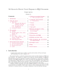


![SWIM User`s Manual (79-pages) [9.8MB - PDF]](http://vs1.manualzilla.com/store/data/005997592_1-d38da0cc1d14ad3dd6bd6e23fa96f310-150x150.png)