Download User Manual book 1 version 2.5

software for the detection and analysis of event clusters
©BioMedware 2012
User Manual
book 1
version 2.5
Copyright 2012, BioMedware, Inc. All rights reserved.
ClusterSeer and BoundarySeer are trademarks of BioMedware, Inc.
Project Leaders: Geoff Jacquez and Leah Estberg
STTR Collaborating Institutions: BioMedware, Inc., the University of Michigan,
and the University of Minnesota.
Software developers: Leah Estberg, Andrew Long, Eve Do, and Bob Rommel.
Manual and help authors: Dunrie Greiling, Leah Estberg, Andrew Long, and
Geoff Jacquez
Advisors: Luc Anselin, Arthur Getis, Dan Griffith, Uriel Kitron, Lance Waller,
and Mark Wilson.
The following individuals provided suggestions and insights that greatly improved
the software: Martin Kulldorff, Peter Diggle, Bruce Levin, Peter Rogerson, and
graduate students and instructors in the course "Spatial Epidemiology" offered in
at the School of Public Health, University of Michigan.
This project was supported by STTR grant #CA64979 from the National Cancer
Institute to BioMedware, Inc. The software and manual contents are solely the
responsibility of the authors and do not necessarily represent the official views of
the National Cancer Institute.
For updated troubleshooting information and FAQs, please visit ClusterSeer
online (http://www.biomedware.com/files/documentation/clusterseer/default.htm).
2
Table of Contents
PREFACE ................................................................................... 10
System requirements ................................................................................ 10
Manual overview ..................................................................................... 11
CHAPTER 1—OVERVIEW ............................................................ 12
About cluster detection ............................................................................ 12
What is a cluster? .............................................................................................12
The classic example..........................................................................................12
Cluster detection methods ................................................................................12
CDC guidelines........................................................................................ 13
CDC multi-step approach.................................................................................13
Limits of cluster detection ........................................................................ 14
Disease risk and relative risk .................................................................... 15
STATISTICAL CONCEPTS ................................................................. 16
About statistical methods ......................................................................... 16
P-values ................................................................................................... 17
Poisson null models ................................................................................. 18
Poisson point processes ....................................................................................18
z scores .................................................................................................... 19
Interquartile distance................................................................................ 19
MONTE CARLO RANDOMIZATIONS ................................................. 20
About Monte Carlo randomization .......................................................... 20
Calculating Monte Carlo P-values ............................................................ 20
Types of randomization ........................................................................... 21
Conditional randomness .......................................................................... 21
Multinomial randomization ..................................................................... 22
Poisson randomization............................................................................. 22
Generating Poisson random variables ...............................................................22
SPATIAL AND TEMPORAL CONCEPTS .............................................. 23
Extrapolation from census data ................................................................ 23
Neighbor relationships ............................................................................. 24
Contiguity matrix.............................................................................................24
3
Polygon overlap .......................................................................................25
Polygon contiguity ...................................................................................25
Rook vs. queen ................................................................................................25
CHAPTER 2—WORKING IN CLUSTERSEER.................................. 26
Session log ...............................................................................................27
Editing ............................................................................................................27
Printing ...........................................................................................................27
Exporting ........................................................................................................27
Plots.........................................................................................................28
Formatting and editing axis labels ....................................................................28
Formatting axis scaling and points ...................................................................28
Axes........................................................................................................................28
Points ......................................................................................................................28
Exporting ........................................................................................................28
Histograms ...............................................................................................29
Formatting and editing axis labels ....................................................................29
Formatting axis scaling and bars ......................................................................29
Axes........................................................................................................................29
Bars.........................................................................................................................29
Exporting ........................................................................................................29
MAPS............................................................................................. 30
Maps overview .........................................................................................30
The left panel: the map layers...........................................................................30
The right panel: the map itself ..........................................................................31
The map toolbar .......................................................................................32
Working with maps ..................................................................................33
Changing the order of data layers .....................................................................33
Deleting map layers .........................................................................................33
Removing maps...............................................................................................33
Exporting maps ...............................................................................................33
Querying maps .........................................................................................34
Formatting maps ......................................................................................35
Point layer properties................................................................................35
Polygon layer properties ...........................................................................36
Line style.........................................................................................................36
4
Fill color ..........................................................................................................36
Single color.............................................................................................................36
Categorical..............................................................................................................36
Graduated color ......................................................................................................36
RGB........................................................................................................................36
Transparent.............................................................................................................36
CHAPTER 3—SUBMITTING DATA ............................................... 37
Data overview.......................................................................................... 37
Spatial data......................................................................................................37
Temporal data .................................................................................................37
Spatio-temporal data ........................................................................................37
Data types................................................................................................ 38
About submitting data.............................................................................. 38
Data formats—general ............................................................................. 39
Spatial data formats ................................................................................. 40
Temporal data formats ............................................................................. 40
Coordinate system ................................................................................... 41
Missing data ............................................................................................ 41
FILE TYPES .................................................................................... 42
Text files .................................................................................................. 42
Text file guidelines ................................................................................... 42
Shapefile import requirements.................................................................. 43
Contiguity files......................................................................................... 43
Binary contiguity relationships (*.gal). ...........................................................43
CHAPTER 4—DISEASE CLUSTER METHODS ................................ 45
Retrospective surveillance ........................................................................ 45
Spatial clusters ......................................................................................... 46
Global spatial methods.....................................................................................46
Local spatial methods.......................................................................................47
Focused spatial methods ..................................................................................47
Space-time clusters ................................................................................... 47
Temporal clusters..................................................................................... 48
5
CHAPTER 5—BESAG AND NEWELL'S METHOD ........................... 49
Besag and Newell's method: Statistics.......................................................50
Test statistics ...................................................................................................50
Notes...............................................................................................................50
Besag and Newell's method: l....................................................................51
Besag and Newell's method: r ...................................................................52
Besag and Newell's method: How to.........................................................53
Besag and Newell: Results ........................................................................55
Distribution .....................................................................................................55
Map ................................................................................................................55
Session log.......................................................................................................55
CHAPTER 6—BITHELL'S LINEAR RISK SCORE TEST..................... 57
Bithell's Test: Statistic ...............................................................................58
Test statistic.....................................................................................................58
Conditional and unconditional tests .................................................................59
Bithell's Test: Relative risk functions .........................................................60
Bithell's Test: Choosing parameters ..........................................................62
Beta—the intercept ..........................................................................................62
Phi—distance decay.........................................................................................62
Bithell's Test: How to ...............................................................................63
Bithell's Test: Results ................................................................................65
Distribution .....................................................................................................65
Map ................................................................................................................65
Plot .................................................................................................................65
Session log.......................................................................................................66
CHAPTER 7—DIGGLE'S METHOD ............................................... 67
Diggle's Method: Statistic .........................................................................68
Test statistic.....................................................................................................68
Diggle's raised density model....................................................................69
Diggle's Method: Choosing initial parameters ...........................................70
Diggle's Method: GLRT ...........................................................................71
Diggle's Method: MLE .............................................................................71
Diggle's Method: How to..........................................................................72
6
Diggle's Method: Results.......................................................................... 73
Plot..................................................................................................................73
Map.................................................................................................................74
Session log .......................................................................................................74
CHAPTER 8—KULLDORFF'S SCAN .............................................. 75
Kulldorff's Scan: Statistic (Poisson) .......................................................... 76
Test statistic .....................................................................................................76
Likelihood ratio ...............................................................................................76
Kulldorff's Scan: How to .......................................................................... 77
Kulldorff's Scan: With census file ............................................................. 77
Kulldorff's Scan: With population-at-risk data .......................................... 79
Kulldorff's Scan: Results........................................................................... 80
Distribution .....................................................................................................80
Map.................................................................................................................80
Plot..................................................................................................................81
Session log .......................................................................................................81
CHAPTER 9—LEVIN AND KLINE'S MODIFIED CUSUM ................. 83
Levin and Kline's Modified CuSum: Statistic ........................................... 84
Test statistic .....................................................................................................84
Levin and Kline's Modified CuSum: How to ............................................ 85
Levin and Kline's Modified CuSum: Single file ........................................ 85
Levin and Kline's Modified CuSum: Two files ......................................... 86
Levin and Kline's Modified CuSum: Results ............................................ 88
Distribution .....................................................................................................88
Plot..................................................................................................................88
Session log .......................................................................................................88
CHAPTER 10—LOCAL MORAN TEST ........................................... 89
Local Moran: Statistic .............................................................................. 90
Test statistic .....................................................................................................90
Significance .....................................................................................................90
Local Moran: How to .............................................................................. 91
Local Moran: With Shapefile ................................................................... 91
Local Moran: With two files .................................................................... 92
Local Moran: Results ............................................................................... 93
7
Distribution .....................................................................................................93
Map ................................................................................................................93
Session log.......................................................................................................93
CHAPTER 11—RIPLEY'S K-FUNCTION ......................................... 95
Ripley's K-function: Statistic.....................................................................96
Test statistic.....................................................................................................96
Evaluating the K-function ................................................................................96
Monte Carlo randomizations ...........................................................................97
Ripley's K-function: Edge correction.........................................................97
Ripley's K-function: How to .....................................................................98
Ripley's K: Results....................................................................................99
Map ................................................................................................................99
Plot .................................................................................................................99
Session log..................................................................................................... 100
CHAPTER 12—ROGERSON'S METHOD .......................................101
Rogerson's Method: Statistic...................................................................102
Test statistic................................................................................................... 102
Modified Tango statistic................................................................................. 102
Cumulative sum approach ............................................................................. 102
Rogerson's Method: Choosing parameters ..............................................104
Change threshold: k ...................................................................................... 104
Critical value: h ............................................................................................. 104
Risk weight: Tau ........................................................................................... 104
Batch size: n .................................................................................................. 104
Rogerson's Method: How to ...................................................................105
Rogerson's Method: Results....................................................................106
Map .............................................................................................................. 106
Plot ............................................................................................................... 106
Session log..................................................................................................... 106
CHAPTER 13—SCORE TEST........................................................ 108
Score: Statistic ........................................................................................109
Test statistic................................................................................................... 109
Variance ........................................................................................................ 109
Score: How to ........................................................................................110
8
Score: Results......................................................................................... 112
Distribution ...................................................................................................112
Map...............................................................................................................112
Plot................................................................................................................112
Session log .....................................................................................................113
CHAPTER 14—TURNBULL'S METHOD ........................................114
Turnbull's Method: Statistic ................................................................... 115
Test statistic ...................................................................................................115
Turnbull's Method: How to .................................................................... 116
Turnbull's Method: Results .................................................................... 117
Distribution ...................................................................................................117
Map...............................................................................................................117
Session log .....................................................................................................118
CHAPTER 15—MULTIPLE COMPARISONS...................................119
Multiple Comparisons: Statistics ............................................................ 120
Adjusted significance levels ............................................................................120
Combined P-values ........................................................................................120
Multiple Comparisons: How to .............................................................. 121
Multiple Comparisons: Results............................................................... 122
RESOURCES ..............................................................................123
Troubleshooting ..................................................................................... 123
Data import errors .........................................................................................123
References ............................................................................................. 123
Glossary................................................................................................. 127
Index ..................................................................................................... 133
9
Preface
ClusterSeer supplies data visualization tools and state-of-the-art statistical methods
to explore spatial and temporal patterns of disease.
ClusterSeer methods can be used to investigate disease clusters in space, in time,
and spatial clusters that depend on time (spatio-temporal interaction).
Use the method of your choice, or find an appropriate method using the
ClusterSeer Advisor.
System requirements
10
•
Windows 95 or Windows NT 4.0 or more recent operating system
•
Screen resolution of 800 x 600 or finer for best viewing of the maps and
graphics
•
256 colors or better highly recommended for graphics
Manual overview
This manual outlines how to use ClusterSeer, BioMedware’s tool for detecting pattern
in health data.
Chapter 1 presents the conceptual background for the software. This chapter
includes a cluster definition and a perspective on the role of cluster detection in the
larger process of identifying the source of disease. It also surveys concepts in
epidemiology, spatial analysis, temporal analysis, and statistics used in
ClusterSeer.
Chapter 2 provides an overview of how to use ClusterSeer and what tools are
available for viewing your data and results. Chapter 3 details how to submit files
and data file and format requirements. Chapter 4 describes the heart of
ClusterSeer: cluster detection methods. You may read this section to choose a
method, or you can use the Cluster Advisor available within the software.
Chapters 5-14 detail individual statistical methods, while Chapter 15 describes the
multiple comparisons feature.
The manual also has a resources section that includes a glossary, troubleshooting,
references, and an index.
For easier differentiation of interface and description, this manual will use the
following style conventions:
Typeface
Meaning
serif type
explanatory text
sans serif type
part of the ClusterSeer interface, such as
menu items or dialogs
This information is also available in online help ("CSeer Help.chm"), accessible
from the "Help" menu and "Help" buttons on dialogs in ClusterSeer. The online
help has hyperlinks that connect related topics.
BioMedware also has a ClusterSeer Online page on its website,
http://www.biomedware.com/files/documentation/clusterseer/default.htm.
Please check this for updates and additional information.
11
Chapter 1—Overview
ClusterSeer offers statistical methods for the analysis of health data. Using
ClusterSeer will draw on your understanding of concepts in epidemiology, spatial
analysis, temporal analysis, and statistics.
About cluster detection
What is a cluster?
A cluster is an aggregation of disease in space, in time, or in both space and time.
Cases of a disease can be referenced to a specific location, such as a residence, and
time, such as the date of diagnosis. Disease clusters occur when more cases are
identified at a particular place and/or time than would otherwise be expected. The
study of disease clusters may suggest possible factors and exposures influencing
risk for a disease. More likely, cluster identification will provide incentive to
undertake a comprehensive epidemiological study.
The classic example
Dr. John Snow's study of the 1854 London cholera outbreak is an historic example
of a cluster analysis that suggested an effective intervention. In brief, the outbreak
of cholera was detected by Dr. Snow even before the bacterium that causes cholera
had been identified. He mapped mortality and found that most deaths occurred
near the Broad Street Pump. Once the handle of the pump was removed, the
outbreak subsided.
Cluster detection methods
Since the time of the London cholera outbreaks, more sophisticated statistical
analyses have been developed to detect clustering. Advances in computer
databases, Geographic Information Systems, and statistical techniques have
augmented our toolbox for the study of disease clusters. Many of the methods
offered in ClusterSeer are very new, developed in the last decade.
Cluster statistics offer criteria to determine when observed patterns of disease
significantly depart from expected patterns. ClusterSeer includes methods that
explore different kinds of clustering: spatial, temporal, and space-time clusters.
Many of the methods in ClusterSeer use Monte Carlo randomization techniques to
evaluate observed values. These computationally intense methods are more
available now that a computer can quickly randomize datasets and perform the
calculations.
12
CDC guidelines
The Centers for Disease Control and Prevention (CDC) advocate a multi-step
approach for investigating disease clusters (1990). ClusterSeer offers tools for the
cluster assessment stage, steps 2a and 2c.
CDC multi-step approach
1.
Initial contact and response. An agency is notified of a perceived cluster;
it then decides whether further evaluation is necessary.
2.
Cluster assessment.
a.
Preliminary evaluation. This step provides a rough estimate of the
probability of the perceived cluster occurring by chance. In this step,
determine the geographic area and time to examine and find a
reference population for comparison. Then, calculate statistics for the
perceived cluster and compare them to the reference population.
b.
Case evaluation. Verify the case reports are accurate.
c.
Occurrence evaluation. A more thorough descriptive evaluation,
repeating the preliminary evaluation with verified data. This step also
includes a literature review to investigate an association between the
cluster and exposure or source.
3.
Major feasibility study. Here, a case-control study is designed and any
environmental monitoring scheme planned.
4.
Etiologic investigation. This step implements the study planned in Step
3. It evaluates the link between the hypothesized cause of the cluster and
the disease. It does not necessarily give information on the causes of the
original cluster, but evaluates plausible causes.
Most studies of apparent disease clusters are not substantiated after early data
exploration. Most end at stage 2, after finding no significant clustering. For
example, The Minnesota Department of Health received 420 reports of apparent
clusters between 1981-8 (Bender et al. 1990). About 95% of these investigations
were ended at stage 2, with no clustering found. Of the remaining 5%, only 1/5, or
1% of the original total, warranted an epidemiological study. A similarly low rate
of cluster verification occurred in a study of 61 cluster investigations between 197884 at the National Institute for Occupational Safety and Health (Schulte et al.
1987). Most apparent clusters did not have a greater than expected number of
cases, and of those that did, most could not be explained by occupational
exposure.
13
Limits of cluster detection
ClusterSeer provides statistical methods for evaluating disease clusters
quantitatively. Most statisticians and researchers consider cluster detection
methods as more suitable for exploratory data analysis than rigorous hypothesis
testing.
As is clear from the CDC guidelines for cluster investigations, the study of disease
clusters often occurs with incomplete knowledge. Spatial locations of cases often
simply serve as a proxy or indirect estimation for exposure to a risk factor. The
causes of a disease cluster may not yet be understood or even identified.
Additionally, the precise date of disease onset is often unavailable and may be
estimated with date of diagnosis or onset of symptoms. Because of this incomplete
knowledge, cluster detection methods can better help identify patterns and
generate hypotheses rather than formally test pre-existing hypotheses.
Once the hypotheses are generated, they need to be tested with additional,
independent data. Otherwise, the procedure is somewhat circular, testing for
patterns we have already identified. Thus, cluster detection/assessment is a step
towards understanding spatial and temporal patterns in health data, rather than an
endpoint in the process. It can be used in planning subsequent studies, such as
case-control studies and environmental monitoring schemes.
14
Disease risk and relative risk
Risk may be defined as the average probability of disease developing in an
individual during a specified time interval. It may be estimated by dividing the
number of disease events by the number of subjects at risk in a specified time
interval. Yet, drawing individual-level conclusions about risk from group-level data
has its limits (Morgenstern 1998).
Relative risk (RR) is often estimated for a sub-group of study subjects as the ratio
of that group's average risk to a baseline measure of disease risk. In those cases
when an appropriate referent group cannot be identified, either the average risk
over the entire set of study subjects or a national average may be used as the
baseline risk for comparison.
Some of the spatial methods require an understanding of risk or relative risk as a
function of space. Suppose that exposure to a point source (focus) elevated the risk
for a particular type of disease, and distance to the point source served as a proxy
estimate of the amount of exposure experienced. We could create a function by
which degree of exposure would be estimated according to distance from the focus
(postulated degree of exposure). The RR could peak at the point source, and
decline with increasing distance. It may be difficult to anticipate the appropriate
model form, and the fit of the final model to the actual data should be considered.
However, please note, using the observed spatial disease pattern to estimate the
risk or RR function is circular and invalidates statistical inference. A priori
knowledge should contribute to the specification of the function parameters.
15
STATISTICAL CONCEPTS
About statistical methods
The methods in ClusterSeer evaluate spatial, temporal, and spatio-temporal
disease clusters. The fundamental question behind all these methods is whether the
pattern of the data is clustered. All the methods evaluate hypotheses; though these
hypotheses are better considered exploratory, see Limits of cluster detection. The
hypotheses differ between methods, but all the methods can be characterized using
the following structure (from Waller and Jacquez 1995):
•
The null spatial model defines the distribution of cases of the disease
expected without clustering. This distribution may be spatial, temporal, or
spatio-temporal depending on the method, question, and data.
•
The null hypothesis is a prediction about spatial pattern based on the null
spatial model.
•
The test statistic summarizes an aspect of the data of biological or
epidemiological interest.
•
The null distribution of the test statistic can be derived theoretically or
empirically through Monte Carlo randomization. Example theoretical
null distributions include the Poisson null distribution. Either way, the
null distribution reflects the null spatial model.
•
The alternative hypothesis is a counter to the null hypothesis, a different
prediction defined either in the terms of the null spatial model or in terms
of additional parameters to define "clustering."
•
The alternative spatial model can be very basic and somewhat vague "not
the null spatial model," or it can be a more specific model defining a
particular model of disease distribution.
Probability values (P-values) for the observed test statistics can be obtained by
comparing them to the null distribution. This comparison gives a quantitative
estimate of the probability of the observed value under the null hypothesis.
16
P-values
P-values, short for probability values, provide an estimate of how unusual the
observed values are. The P-value of a test statistic can be obtained by comparing
the test statistic to its expected distribution under the null hypothesis (the null
distribution).
The interpretation of a test statistic balances the possibility of two types of errors.
Declaring whether a P-value is statistically significant involves choosing the level
of error with which you are comfortable. Alpha provides the threshold for
significance. If the P-value for the observed value falls below alpha, then the
observation is termed significant.
concept
symbol or formula
meaning
type I error
, alpha (also called
significance level)
the probability of rejecting the null
hypothesis when it is true
type II error
, beta
1-
statistical
power
the probability of accepting the null
hypothesis when it is false
the power of a test indicates its ability to
reject the null hypothesis when it is false
P = 0.05 is the traditional alpha level, which can be interpreted to mean that results
that are more extreme would occur by chance less than 5% of the time, if the null
hypothesis were true. The figure below graphs 1,000 Poisson random numbers
(lambda = 3). The thin line illustrates the P = 0.05 alpha level for a one-tailed test.
The P-value is less than alpha when the test statistic is higher than that cutoff. In
that case, it is customary to reject the null hypothesis and accept an alternative
hypothesis, that there is clustering.
Poisson Distribution, lambda = 3
frequency
300
200
100
0
0 1 2 3 4 5 6 7 8 9 10
Most ClusterSeer methods
are one-tailed, focusing on
the upper-tail of the
distribution. They test
whether the test statistic is
higher than expected. Twotailed tests evaluate whether
the statistic diverges from a
central value, and the alpha
level is divided between the
two tails of the distribution.
17
Poisson null models
The null hypothesis of a Poisson disease rate is usually a good representation of
randomly distributed non-infectious rare diseases (Waller and Jacquez 1995). It is
used in many cluster detection methods in ClusterSeer, including Besag and
Newell's method. A Poisson function can be described by one parameter, lambda
( ), the mean and variance of the distribution. Two Poisson distributions are
illustrated below, each with a different lambda value. Within ClusterSeer, lambda
is the average or expected case count, calculated from the average or expected
disease frequency multiplied by the population-at-risk.
Lambda = 2
Count
40
20
0
0
3
6
9
12
Value
Lambda = 5
Count
40
20
0
0
3
6
9
12
Value
Poisson point processes
Poisson point process models are used for null and alternative spatial models in
Diggle's Method and Ripley's K-function. Poisson point processes produce sets of
points with a given intensity ( , the mean and variance of the Poisson
distribution), an expected number of points or cases per unit area.
18
z scores
Z scores calculate a standardized difference between the observed and expected
value of a statistic:
(I − E(I ))
z=
Var (I )
In this case, I is the statistic, E(I) is the expected value of I, and Var(I) is the
variance of I. Z scores are distributed approximately normally, with a mean of 0
and a variance of 1.0.
Interquartile distance
The interquartile distance is used to find outliers in the local Moran test. The
interquartile distance is the difference between the values for the 25th-percentile
and the 75th-percentile of the test statistic.
To obtain these values, ClusterSeer orders the test statistics from smallest to
largest. The 25th percentile value is the test statistic that divides the ordered set such
that 25% of the statistics are smaller and 75% are greater than that value. The 75th
percentile value is the test statistic that divides the ordered set such that 75% of the
statistics are smaller and 25% are greater. If the number of test statistics cannot be
evenly divided by two, these values are calculated as the mean of the two test
statistics closest to the appropriate position.
ClusterSeer then multiplies the interquartile distance by 1.5. Any values farther
from the median than 1.5 times the interquartile distance are considered outliers.
median
percentile: 25th
75th
interquartile distance
19
MONTE CARLO RANDOMIZATIONS
About Monte Carlo randomization
Monte Carlo randomization is one way to quantitatively evaluate observed data
and test statistics.
In general, Monte Carlo Randomization (MCR) procedures follow this sequence:
1.
Following the calculation of a statistic from the original dataset,
observations are randomized.
2.
The statistic is recalculated for the randomized data.
3.
Steps 1-2 are repeated a given number of times, amassing distributions
that will be used to calculate P-values for the observed statistic.
4.
P-values are calculated by comparing the observed statistic to the
reference distribution.
ClusterSeer randomizes the original dataset according to the approach
recommended for a particular method (see Types of randomization). Null
hypotheses and the randomization approach are detailed in individual method
descriptions.
Calculating Monte Carlo P-values
The P-value is the relative ranking of the test statistic among the sample values
from the Monte Carlo randomization. You can calculate P-values to see whether
observed values are unusually large or small for the null distribution. This
calculation compares the observed value to the upper and the lower tails of the null
distribution. Most tests in ClusterSeer explore whether the observed value is
unusually large for the distribution, using Pupper only.
Pupper =
NGE + 1
Nruns + 1
Plower =
NLE + 1
Nruns + 1
where Nruns is the total number of Monte Carlo simulations, NGE is the number of
simulations for which the statistic was greater than or equal to the observed
statistic, and NLE is the number of simulations for which the statistic was lower
than or equal to the observed statistic. One (1) is added to the numerator and
denominator because the observed statistic is included in the reference distribution.
20
Types of randomization
"Randomization" is a broad term, used differently in different contexts. Within
ClusterSeer, randomization methods vary between methods. For the multinomial
and Poisson distributions, ClusterSeer generates random values by choosing values
from the specified distribution. For conditional randomness, data values are
reassigned among sub-groups.
Randomization Technique
Cluster Detection
Method
Conditional randomness
Local Moran
Drawing from a multinomial distribution
Besag and Newell
Bithell—conditional
Kulldorff's Scan
Turnbull
Drawing from a Poisson distribution
Bithell—unconditional
CuSum
Score
Alter distances between points by multiplying their
locations by a random number
Ripley's K function
Conditional randomness
This approach is used to redistribute disease frequency values among spatial
regions in the Local Moran method (Anselin 1995). In each randomization, the
disease frequency is held fixed for one spatial region, and the remaining values are
randomly assigned new locations. Thus, the randomness is conditional—all
regions receive randomized frequencies but one. This process is repeated as each
region is evaluated in turn.
21
Multinomial randomization
A multinomial distribution describes the outcomes of independent trials with two
or more possible, mutually exclusive outcomes. This approach is used to
redistribute cases of disease among spatially or temporally referenced sub-groups
(bins) under analysis. Cases are distributed at random among bins, where the
probability of a case being placed in a particular bin is proportional to the
population-at-risk size in that bin.
The figure below shows a simple example of this process. There are four bins (a, b,
c, and d) that have population sizes of 10, 50, 20, and 20. The interval from 0-1 is
partitioned among them, with each bin getting an interval proportional to its
relative size (so 1/10, 1/2, 1/5, and 1/5 respectively). Then, as a random number
generator supplies values between 0-1, each value falls into a particular bin and
counts as a case in that bin.
0
1
bins: a b c d
This randomization technique is used in Besag and
Newell's, Bithell's—conditional, Kulldorff's Scan, and
Turnbull's methods.
Poisson randomization
This Monte Carlo randomization approach redistributes cases of disease among
spatially or temporally referenced sub-groups using Poisson random variables. This
approach is used in the Score, Bithell—unconditional, and CuSum methods.
Generating Poisson random variables
Count
This method generates randomized case counts drawing from Poisson
distributions. The shape of the Poisson distribution depends on one parameter,
(lambda), its mean and variance (see example Poisson distribution below). In this
case, is set using the
expected case count for
Lambda = 2
that subgroup (region or
time period), the product
40
of the population-at-risk
20
and the average or user0
specified baseline risk.
0
3
6
9
12
Value
22
SPATIAL AND TEMPORAL CONCEPTS
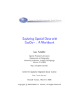
Extrapolation from census data
ClusterSeer can extrapolate population-at-risk counts from census data. This
feature can be used in Kulldorff's Scan, Rogerson's, and CuSum methods.
ClusterSeer offers two extrapolation methods, step and linear extrapolation.
population size
census value
extrapolation
step
linear
both
1980
1990
2000
years
Step
The population-at-risk count is assumed equal to the immediately
preceding census count. It will change with the next provided census
value.
Linear
The population-at-risk count is estimated assuming a linear change in
population between the two nearest census figures. Population-at-risk
values are estimated along the line connecting the two census values.
for both
methods
Dates before the first census value will be set to the first value. Dates
after the final census value will be set to the last value.
Census dates are specified on a yearly scale. The extrapolation will be
estimated at the temporal scale used for the case data (daily, weekly,
monthly, or yearly).
23
Neighbor relationships
Neighbor relationships between regions underlie statistical methods such as local
Moran. To examine spatial association, you first need to define how ClusterSeer
should set neighbor, or contiguity, relationships. Exactly what is next to what?
ClusterSeer can set neighbor relationships in two ways: 1) using lists of neighbors
for each region from SpaceStat™ sparse ASCII files or 2) based on polygon
contiguity from a GIS file.
Contiguity matrix
ClusterSeer uses either data file to create a contiguity matrix holding binary spatial
weights. These weights indicate whether regions neighbor each other. The weight
between two areas that share a common border is set to 1. The weight between two
areas that do not share a common border is set to 0.
The figure below illustrates a simple example of three polygons and their
contiguity matrix. The first row in matrix a describes neighbor relationships for
polygon 1 (it cannot neighbor itself, so the first value is zero, it neighbors polygon
2, so the second value is 1, and it does not neighbor polygon 3, another zero.).
Lower rows describe polygons 2 and 3 in turn.
For local Moran, ClusterSeer row-standardizes spatial weights stored in the
contiguity matrix. Row-standardizing matrix a leads to matrix b. For example, as
polygon 2 has two neighbors, each neighbor is weighted ½, so weights in the row
add up to 1 and the statistic is not biased by the number of neighboring regions.
1
2
3
0 1 0ù
é 0 1 0 ù
a) éê
ú b) ê
ú
ê 1 0 1ú
ê0.5 0 0.5ú
êë0 1 0úû
êë 0
1
0 úû

SpaceStat™ was developed by Luc Anselin, and it is distributed by BioMedware,
Inc.
24
Polygon overlap
If your polygons overlap, it may be difficult to view them when mapped or to
select them for queries. ClusterSeer will not be able to display properly shaded
areas where overlap occurs. Uniquely named polygons completely contained
within another polygon will be correctly processed for analysis and display.
Relatively smaller, non-uniquely named polygons will be discarded on import and
excluded from the analysis.
Polygon contiguity
ClusterSeer can derive neighbor relationships from a file of polygons. In essence,
ClusterSeer will evaluate whether the polygons share a border with each other. If
they share a border, they are considered neighbors. In order to derive neighbor
relationships from polygons in shapefile format, you must specify how ClusterSeer
should evaluate these relationships. While it may seem like a trivial concept, in
fact the specification of neighbor relationships can influence the outcome of
statistical analyses.
Rook vs. queen
Two options are available—rook and queen—their names come from the
movements of chess pieces. The rook can only move to squares that share a border
of some length with its current square. In the figure below, the rook, illustrated as
the gray circle, can only move to the four black squares. The queen can move to
any square that shares even a point-length border. So, she can move to the rook's
squares and any square that shares a corner (one vertex) with her current square. If
the gray circle illustrated the queen's position, the queen could move to any of the
eight adjacent squares.
Thus, rook is a more stringent definition of polygon contiguity than queen—for
rook, the shared border must be of some length, whereas for queen the shared
border can be as small as one point.
25
Chapter 2—Working in ClusterSeer
ClusterSeer workflow is organized around the methods themselves. The general
framework is the same for all methods: you specify a method, you supply data,
ClusterSeer performs an analysis, and then you may view the results of the
analysis.
When you open ClusterSeer, a session log is opened at the same time. It will serve
as a text-based view for reporting results of all analyses in a single ClusterSeer
session. As you perform new analyses, information on them is appended to the
existing log.
Graphical views can help visualize the results of an analysis, and so they are only
available once you have imported data and performed an analysis. Graphical
views reflect the most recent analysis. No record of maps, histograms, and plots
from previous analyses will remain. To view them again, you must recreate them.
Open always,
records all activities
Available after an analysis,
displays the most recent results
Session Log
Plots
Histograms
Maps
26
Session log
ClusterSeer records text-based information from your analyses in the memo screen
within the main window, the session log. Information recorded includes the name
and date last modified of the data files, results from each analysis, and results from
multiple comparison adjustments.
During data exploration and analysis, you may find it useful to edit or print the
text on this page. You may export the log as a plain text file (*.txt) for opening in
other applications.
Editing
You may also add references or notes directly to the session log page by
positioning the cursor and typing.
Printing
To print the log, select "File", then "Print" from the menu. Click "OK" when the
dialog box appears.
Exporting
You can export the log by choosing "Save Log" from the File menu. ClusterSeer
will export the log as a text file (*.txt).
Instead, you may choose to copy a piece of the log to paste into another
application. You can copy sections by selecting them and choosing "Copy" from
the "Edit" menu.
27
Plots
You can use plots to view and interpret the results of the most recent analysis.
After you initiate a new analysis, ClusterSeer will not retain plots from previous
analyses, though you can always recreate them.
Once you have performed an analysis that generates a plot, you may view it by
choosing "Plot" from the "View" menu. Once it is displayed, you may format and
edit axis labels, axis scaling, and points. You can also export plots from
ClusterSeer.
Formatting and editing axis labels
You can format and edit axis labels by double-clicking on the axis. This will call
up a window where you can rename the axis and specify a new font for the label.
Formatting axis scaling and points
You can format the plot by right clicking it and choosing "Change Formatting."
This brings up a formatting window that allows you to change the attributes of the
axes and points on separate tabs.
Axes
To change the scaling on the axes, set the minimum and maximum value shown
for the x- and the y-axes. You may also specify the number of tick marks for each
axis, or you may wish to let ClusterSeer choose the tick marks automatically. To
change the thickness of the axes, choose a line thickness from the pull-down box
next to "Line Thickness:".
Points
You may also change the color of the points. A few different types of points may
be shown on the same plot. Thus, you may want to change the colors and sizes of
the points separately for each kind. Choose the points to change in the pull-down
box after "Data." You may then specify a size and a color for those points.
Exporting
At this point, you cannot export directly from ClusterSeer. To capture your
histogram as a bitmap, take a screenshot of it using the "Print Screen" key. You
can then paste the screenshot into an image editor to view and manipulate it.
28
Histograms
You can use histograms to view and interpret the results of the most recent Monte
Carlo randomizations. After you initiate a new analysis, ClusterSeer will not retain
histograms from previous analyses, though you can always recreate them.
Once you have performed an analysis that includes Monte Carlo simulations, you
may view the histogram by choosing "MC Distribution" from the "View" menu.
Once you are viewing it, you may format and edit axis labels, axis scaling, and
bars. You can also export histograms of Monte Carlo distributions from
ClusterSeer.
Formatting and editing axis labels
You can format and edit axis labels by double-clicking on the axis. This will call
up a window where you can rename the axis and specify a new font for the label.
Formatting axis scaling and bars
You can format the histogram by right clicking it and choosing "Change
Formatting." This brings up the formatting window that allows you to change
the attributes of the axes and the bars on separate tabs.
Axes
To change the scaling on the axes, set the minimum and maximum value shown
for the x and the y-axes. You may also specify the number of tick marks for each
axis, or you may wish to let ClusterSeer choose the tick marks automatically. To
change the thickness of the axes, choose a line thickness from the pull-down box
next to "Line Thickness:".
Bars
You may also change the color of the bars. Up to three colors of bars may be
displayed on one histogram and these can be changed separately (change primary
color, secondary color, or tertiary color). You may also change the number of bins
into which ClusterSeer divides the data.
Exporting
At this point, you cannot export directly from ClusterSeer. To capture your
histogram as a bitmap, take a screenshot of it using the "Print Screen" key. You
can then paste the screenshot into an image editor to view and manipulate it.
29
MAPS
Maps overview
Maps are visual representations of data and statistical results. The map displays the
data and results from the most recent analysis. After you initiate a new analysis,
ClusterSeer will not retain maps from previous analyses, though you can always
recreate them.
Most ClusterSeer maps are displayed in a two-pane window. The left-hand
window lists the active layers in the map, and the right-hand window contains the
map itself.
Some maps, for example those produced by the local Moran method, will have
three panes. In the three-pane maps, the rightmost pane is the map legend.
The left panel: the map layers
This panel lists all the map layers. You may need to expand the frame to view the
full layer names. You may show or hide a map layer by checking or clearing its
associated box using the mouse. Displayed layers have a red check in the box next
to their name.
The active layer is highlighted on the layers list. Click on a layer's name in the
pane to activate it.
The maps are drawn sequentially, with layers higher on the list drawn over those
lower on the list. For instance, if you have a polygon layer it may obscure a point
30
layer underneath it. To fix this, change the order of layers in the layer list. To
change the order of layers on a map, drag layers up or down the list.
The right panel: the map itself
The map panel displays data and results. You may query or reformat active layers.
31
The map toolbar
The map visualization toolbar appears when the map window is active. To
activate the map, click on it.
The "selection" tool is the default tool. In the map layer pane, it can be used
for changing the order of map layers, and activating and deactivating map layers
(see Maps Overview for details). In the map pane, it can be used to select map
features. Using this tool, you can click directly on a feature to select it, or you can
click and drag open a rectangle to select all features that intersect the rectangle.
If you move the arrow to the map pane and right-click, you will have the option of
querying the nearest feature on the active layer (see Querying maps), changing the
properties (color, size of elements) of the active (highlighted) layer, or removing
the active layer from the map.
Use the "zoom" tool to focus on a section of the dataset. Move the tool to
where you want to zoom, and click to zoom in.
Use the "zoom out" tool to enlarge the field of view. Move the tool to where
you want the enlargement to be centered and click to zoom out. ClusterSeer will
not zoom past the spatial extent of the data.
The "zoom to fit" tool returns the visual display to the full spatial extent of
the dataset.
The "pan" tool can be used instead of the scrollbars to move the field of view
across the map. This tool only works when the map is zoomed in somewhat from
the full spatial extent of the data. Click on the button to activate the tool and then
use it to pan the map across the viewing window. For example, to expose a section
to the right of the viewing window, drag the map to the left.
Finally, the "query" button is a method for querying the map; clicking a point
with this tool brings up a table of information about the nearest map feature in the
active layer.
32
Working with maps
ClusterSeer maps are not simply visual displays of data and results—they provide
opportunities for querying the underlying data. Maps are created when ClusterSeer
performs spatial and spatio-temporal analyses on data referenced to spatial
locations. To view the map, choose "Map" from the "View" menu.
If you have performed a sequence of analyses, you can only view the map from the
most recent one. If you have a previous map open when you do a new analysis,
ClusterSeer will remove the previous map. If you need to recreate a map from an
earlier analysis, instruct ClusterSeer to redo the analysis.
Changing the order of data layers
The pane on the left side of the map window lists the map layers. For a layer to be
visible in the map window, its associated box must be checked. Click on the box to
check or clear it. The data layers appear in the order that they are listed, with the
top layer in the list appearing "above" other layers in the view. To change the order
of layers, click on a layer in the list and drag it to where you want it.
Deleting map layers
If you want to completely remove a data layer from a map (not just deactivate it),
highlight the name of the layer, and then hit the "Delete" key. You may also
remove a layer by right clicking on the map and choosing to "Remove this layer
from the map." This procedure removes the active (highlighted) layer.
Removing maps
If you no longer wish to view a map, click on the "close" button
in the map's
upper right corner. You may re-create a map of the most recent analysis by
choosing "Map" from the "View" menu.
Exporting maps
To capture your map as a bitmap, take a screenshot of the map window using the
"Print Screen" key. You can then paste the screenshot into an image editor to
view and manipulate it.
33
Querying maps
Querying calls up information about items on the map.
Click on the query tool and then click on the map. This brings up a table of
information on the nearest feature in the active map layer (the highlighted layer).
The active layer is queried even if it is not currently displayed on the map (checked
in red). To change the active map layer, select a new layer in the map layers pane.
Once you've queried a layer, the queried feature will be recolored orange, and its
table will pop up. This table lists information about the feature. For example, if
you query a point layer, you will get the coordinates of the nearest data point and
any associated data. If you query a circle layer, you will get information on the
circle with the nearest center point.
The queried feature will return to its original color when the query table is closed.
34
FORMATTING MAPS
Formatting maps
To format a map layer, select it on the map layer pane (the selected layer is
highlighted).
Then, call up the properties dialog by right clicking on the map with the
selector and choosing "Properties" from the pull-down menu.
Because formatting options change with the layer type, read up on formatting
individual layers:
•
point and
•
polygon map layers
Point layer properties
You can choose the size of the points by specifying their radius in pixels. You can
change the color of the points by clicking the "Change Color" button and
choosing a new color.
Hit "Update" to apply any changes you make. Choose "Cancel" to keep the
current formatting.
35
Polygon layer properties
You may change the outline style and the fill colors of polygon layers. Hit "OK" to
apply any changes you make. Choose "Cancel" to keep the current formatting.
Line style
You can choose the width of the lines and their color. Choose line width from the
drop-down box and line color using the "Change Color" button.
Fill color
Single color
Choose this option to color all polygons the same. Change the color by hitting
"Change Color" and picking a new one from the palette.
Categorical
You can choose to color the map based on the values of one categorical variable.
Choose the variable from the pull-down list. ClusterSeer will choose the color
automatically.
Graduated color
You can choose to display the values of a single variable using a gradient between
two colors. You can choose a minimum and a maximum color (the minimum
value will be displayed as the minimum color, and the maximum value as the
maximum color, with intermediate values a blend).
To change the variable displayed, choose another from the pull-down list. You
also may change the minimum and maximum colors.
RGB
You may choose to represent the values of up to three variables using red, green,
and blue. You specify the value associated with each color.
Transparent
You can also color them all "transparent." Transparent fill lets information from
underlying map layers come through, if more than one layer is present.
36
Chapter 3—Submitting Data
ClusterSeer provides analytic methods for exploring spatial and temporal trends in
health data. It offers a number of state-of-the-art methods for cluster detection as
well as data and results visualization.
The method you select determines the data types and format required, what
parameters you need to enter, and what output is available to view.
Data overview
ClusterSeer analyzes pattern in spatial and spatio-temporal data. These methods
analyze study subjects, such as cases and susceptible individuals, as study units
described at the individual or group level.
Spatial data
Study units may have associated spatial information, expressed as point locations
or areas. Data on individuals can be fixed to a point location, such as a workplace
or residence. Group-level data is often aggregated over a region, a wider spatial
area such as a township or county. This area may be represented as a point (often
the region's centroid) or an area (a polygon). See spatial data formats.
Temporal data
Study units may have associated temporal information. These temporal references
can represent either a point in time or an interval of time. For individuals, time
point may indicate the date of diagnosis or symptom onset. For groups, time
intervals may be used to aggregate study subjects into time-dependent collections
of individuals. See temporal data formats.
Spatio-temporal data
Study units may have associated spatial and temporal information. In order to
minimize data repetition, several input files may be required. See formats for both
spatial and temporal data.
37
Data types
ClusterSeer can analyze individual- and group-level data. Different methods are
appropriate to different data and analysis types.
Individual-Level—The unit of observation and analysis is the individual study
subject. Currently, ClusterSeer offers methods for surveillance and spatial cluster
analysis of individual-level data. Data can consist of the locations or time
references for individuals with (cases) or at risk for (controls) the health outcome
under investigation.
Group-Level—The unit of analysis is a group of study subjects aggregated within
geographic regions and/or temporal intervals. Spatial and spatio-temporal cluster
detection can be conducted on group-level data. ClusterSeer also offers two
retrospective surveillance methods for temporal and spatial clustering of grouplevel data, though Rogerson's Spatial Pattern Surveillance method also requires
individual level data. The data often consist of disease frequency estimates or case
and population-at-risk counts for each group.
The location of spatially aggregated data may have to be simplified for analysis. In
practice, these areas can be represented with a single point location, such as the
geographic center (centroid) for group-level data.
About submitting data
ClusterSeer currently requires specific file structures for each method, though we
intend to relax this restriction in future versions. For plain text data files, the data
for each unit of analysis (individuals or groups) are stored on separate file lines as
records. Currently, ClusterSeer expects the record data in a particular order, such
as label first, then x-coordinate, then y-coordinate, then case count, then
population-at-risk count. Required file structures are detailed in the "How to"
section for each method.
Must ClusterSeer data files will be expected in plain text format. Shapefiles and
SpaceStatTM sparse ASCII files are used to specify neighbor relationships for local
Moran.

SpaceStatTM was developed by Luc Anselin, and it is distributed by BioMedware,
Inc.
38
Data formats—general
Spatial, temporal, and other data must follow specific data formats to be read by
ClusterSeer.
Duplicate spatial locations and/or temporal references should not be submitted for
aggregate data (such as regions and associated centroids or temporal intervals).
Additionally, all census years submitted as temporal references for population-atrisk sizes should be unique. Duplicate points in space and time can be submitted to
indicate individual subject locations and times of events.
Type
Format
Valid
range
Case count or
Positive numbers, can include fractions.
disease frequency
0 to 3.4 x
1038
Population-at-risk Positive numbers, can include fractions.
count
1 to 3.4 x
1038
Categorical
variables
(such as
case/control
status)
Represented by whole numbers, such as 0 or 1. Can not
be submitted as decimal values (such as 1.000) if
applicable
they match expected codes once truncated.
Labels
(for regions or
individuals)
Labels must be unique. Label matching between
not
files is case-sensitive.
applicable
Can be numbers, letters, or a combination.
Can include spaces if the label is enclosed in single
or double quotation marks.
39
Spatial data formats
Data can be imported in planar or geographic coordinates. Planar coordinates
must be expressed as numeric values. Geographic coordinates must fall within the
following range:
Valid range
Latitude
-90 to +90
Longitude -180 to +180
When the coordinates describe region centroids used to aggregate study units, the
data is checked on import for duplicate centroids.
Temporal data formats
Sample Format
data
Example Notes
Valid range
Yearly
1998
0001 to 9999
YYYY
Monthly YYYYMM
199801
monthly values (MM) range 000101 to
from 01-12
999912
Weekly YYYYWW
199843
weekly values (WW) range
from 01-52
000101 to
999952
Daily
MM/DD/YYYY 1/2/2001 month and date values may 12/30/1899
be expressed as single digits to
12/31/9999
Userdefined
user-defined
5
positive whole numbers that 0 to 4.2
may represent points in time billion
or non-overlapping,
successive temporal
intervals.
In this scale, the intervals are
naturally ordered by their
magnitude (5 comes after 4)
and there is a known unit
distance between any 2
successive numbers.
40
Census data must be submitted referenced to yearly time units. Data to be
associated with the population-at-risk counts extrapolated from census data must
be referenced to calendar-based units (any system other than user-defined).
Case counts intended to be referenced to populations estimated from census data
are usually aggregated by time intervals. Those intervals containing zero cases
don't have to be specified. If this sort of minimized dataset is submitted and the
temporal range does not match the intended study period span, study period limits
can be explicitly specified in the "Census Data" dialog. For analysis, missing
time intervals in the submitted data set will be filled with case counts equal to zero
and population counts estimated from census data. This approach can be
especially useful for spatio-temporally aggregated data, in which all regions in the
dataset must have the same temporal range.
Duplicate time intervals cannot be submitted for purely temporal analysis. For
spatio-temporal analysis, time intervals can be duplicated across regions, but not
within regions.
Coordinate system
ClusterSeer can import data in planar or geographic coordinates. If you perform a
focused cluster detection method on your data, specify the location of the focus in
the data's original coordinates (i.e. planar coordinates for planar data, geographic
coordinates for geographic data).
•
Planar. This category encompasses all map projections including UTM
(Universal Transverse Mercator) and user-coordinates.
•
Geographic (latitude-longitude). Within ClusterSeer, data in geographic
coordinates are transformed to UTM for calculation and mapping.
o
If your data are in geographic coordinates, you can choose to use
a scale of either meters or kilometers. This scale will be used to
specify distances on the map and in the analyses.
Missing data
Currently, the only type of missing data ClusterSeer can handle is gaps in temporal
intervals. If you have a file with case counts for temporal intervals and you are
using census data for population-at-risk counts, then ClusterSeer will interpret the
missing intervals as having a case count of zero.
Other missing data will prevent file import.
41
FILE TYPES
Text files
ClusterSeer requires most data in ASCII text file format. ASCII or plain text files
can be exported from many spreadsheet and data analysis programs, or you can
create them directly in a text editor.
While the "Select File..." dialog defaults to importing a file with the extension
*.txt, ClusterSeer will import plain text files with any file extension. To import a
file with a different extension, choose "All Files (*.*)" after "Files of type" in
the "Select File...." dialog to view all files. Then, choose the file to import.
Different methods require different file structures. The types of data and their order
in the file is described in the "How to" sections for individual methods. Depending
on the method, the file may contain some or all of these categories: spatial
coordinates, temporal information, and case/disease data.
Text file guidelines
Data for a particular method may be contained in one large file or in several files,
depending on the method's requirements. For several files, consistent labeling is
required to merge the information between files.
Each row in the data file should contain one unit of study. This study unit may be
individual data, count data, or frequency data. Data associated with that study unit
must be in the same row of the text file, delimited by tabs or spaces. Study units
(rows) are separated by a carriage return.
If the data file has more columns than the method requires, additional columns
will be ignored. The relevant columns need to be the first ones, as you currently
cannot choose which columns to import from a text file. If the data file has fewer
columns than the method requires, ClusterSeer will report a data import error.
ClusterSeer does not require a header for the text file.
42
Shapefile import requirements
This file format consists of three separate related files, all with the same file name
but different file extensions (*.shp, *.shx, *.dbf). Once you tell ClusterSeer
where to find the *.shp file, it will look in the same directory for the *.shx and
*.dbf files.
You may import a shapefile for the local Moran test. Once you select the file to
use, ClusterSeer will prompt you to choose region labels and disease frequencies
from column headings in your *.dbf file.
Once you have selected the columns, ClusterSeer loads the data. If you cancel at
this point, the procedure will cancel.
Contiguity files
These files are used to define neighbor relationships in local Moran. Contiguity
files (*.gal) indicate whether areas neighbor each other. Future versions of
ClusterSeer will accept general weight files (*.gwt) to specify more complex
relationships, say based on distance rather than contiguity.
Binary contiguity relationships (*.gal).
These files indicate whether a region has any neighbors, identifying them if so.
These files can be created within and exported from SpaceStatTM, or created
manually in a text editor that can save unformatted, ASCII files.
The *.gal file has the following structure
43
total region count
egolabel
neighbor count
neighbor label
neighbor label......
egolabel
1
neighbor label
egolabel
0
egolabel
neighbor count
etc.
The first row specifies the total region count. ClusterSeer checks for at least one
field in that row, and it verifies that the total region count in the first field matches
the total number of regions specified in the disease frequency data file.
The second row specifies a target region, called an "ego," by its label and a count
of its neighbors.
The third row lists the identities of those neighbors, with the row continuing until
all neighbors have been listed. Egos without neighbors can be specified as having a
neighbor count of zero or be omitted from the list. ClusterSeer checks rows with
neighbor counts for at least 2 fields, checks that the count value is a positive
integer, and that the count is less than the total number of areas minus 1 (because a
region can't be its own neighbor).
The following row specifies the neighbors of the first ego, and there must be at
least as many fields in that row as the neighbor count (excess fields will be
ignored). Neighbor labels cannot match the ego's label, and there can be no
duplicates. If the neighbor count in the previous row is zero, then the next row lists
a new ego and the number of its neighbors.
All region labels (for egos and neighbors) must match those in the disease
frequency file.

SpaceStatTM was developed by Luc Anselin, and it is distributed by BioMedware,
Inc.
44
Chapter 4—Disease Cluster Methods
ClusterSeer offers data visualization tools and state-of-the-art statistical methods to
explore spatial and temporal patterns of disease.
ClusterSeer methods can be used to investigate disease clusters in space, in time, or
spatial clusters that depend on time (spatio-temporal interaction).
To choose a method, you may start with the ClusterSeer Advisor.
In this chapter, you can learn about the methods within ClusterSeer:
•
retrospective surveillance,
•
spatial clustering,
•
o
global,
o
local,
o
focused,
spatio-temporal clustering.
Temporal clustering will be included in the next version of ClusterSeer.
Retrospective surveillance
Retrospective surveillance methods monitor changes in the occurrence of some
event, such as the temporal or spatial pattern of a disease. Surveillance methods
can signal when current conditions differ from a historical baseline (O'Brien and
Christie 1997).
For surveillance, the important steps are determining the baseline rate and the
threshold for alarm—how much change from the baseline is "enough" for concern.
Thus, statistical surveillance methods trade-off sensitivity to changes with the
likelihood of producing a false alarm. Surveillance methods have the highest
accuracy for larger datasets and the highest sensitivity for lower baseline disease
rates (Barbujani and Calzolari 1984).
45
ClusterSeer contains two surveillance methods. Levin and Kline's method analyzes
group-level data, and Rogerson's method requires both individual-level and grouplevel data:
•
Levin and Kline's modified CuSum for temporal surveillance. This
method explores changes in the frequency of an event, such as infection or
a disease.
•
Rogerson's Spatial Pattern Surveillance Technique for spatial surveillance.
This method explores changes in the spatial pattern of an event.
Spatial clusters
These cluster detection methods evaluate whether cases of a disease tend to
aggregate in particular locations. Besag and Newell (1991) classified cluster
detection methods into "general" and "focused" tests. We further subdivide
"general" methods into "local" and "global" categories.
•
•
General methods explore clustering without pre-determined hypotheses
about cluster location.
o
Global methods detect clustering throughout the study area
regardless of their specific locations or spatial extent.
o
Local methods detect clustering limited to geographically
restricted areas within the study.
Focused methods detect clustering around a specific location, such as a
point source exposure to a proposed risk factor.
Global spatial methods
Global cluster detection methods are used to investigate the presence of spatial
patterns anywhere within the study area. They attempt to answer the question: Are
there any unusual disease patterns? These tests focus on whether clustering exists
or not, regardless of location or scope. Essentially, the method evaluates whether a
spatial pattern exists in the data that is unlikely to have arisen by chance. The null
hypothesis for these methods is simply "no clustering exists."
Global cluster methods available in ClusterSeer:
Individual-level data
Ripley's K-function
Group-level data
Besag and Newell's Method
For retrospective surveillance of spatial data, use Rogerson's Method.
46
Local spatial methods
These cluster detection methods are used to investigate spatial disease clusters near
a particular area. They can be thought of as methods that attempt to answer the
question: Are cases neighboring a particular case closer together than expected by
chance?
Local cluster detection methods are available for group-level data only.
•
Besag and Newell's method
•
Turnbull's method
•
Local Moran
Focused spatial methods
These cluster detection methods evaluate spatial disease patterns around a
particular location, or focus. Candidate locations can be used to represent the
position of a proposed risk factor, such as a contaminated well. These methods
attempt to answer the question: Is there a cluster of cases around the identified
location? The null hypothesis for focused tests is "no clustering around the focus".
Focused cluster detection methods available in ClusterSeer:
Individual-level data Group-level data
Diggle's Method
Bithell's method
Score test
Space-time clusters
Spatio-temporal methods detect disease clusters in space that depend on the time
period (Space x Time interaction).
•
Kulldorff's Spatial Scan
47
Temporal clusters
Temporal cluster detection methods are used to investigate disease clusters in time,
whether cases of disease tend to aggregate in particular periods. All are used on
group-level data. These methods can be used to evaluate disease frequency or case
counts in a single or in multiple time series.
The following methods are currently available in BioMedware's Stat! You may
order Stat! or wait until these methods are incorporated into ClusterSeer in the
next release.
Method Disease
frequency
Case count,
single time
series
✓
Dat's Method
Ederer-Myers-Mantel
Method
Empty Cells
Grimson's Method
Larsen's Method
Wallenstein's Scan
48
✓
✓
✓
✓
✓
Case count,
multiple time
series
✓
✓
✓
Chapter 5—Besag and Newell's Method
Besag and Newell's method can detect local or global spatial clusters in group-level
data. When you initiate a Besag and Newell analysis in ClusterSeer, you get both
local and global analysis output. While individual- or case-level analysis is
theoretically possible with this method, ClusterSeer implements only the regioncentered group-level technique.
This method scans the data for collections of cases that appear to be unusual
clusters. To do so, it centers a circular window on each region in turn. This
window is then expanded to include neighboring regions until the total number of
cases in the window reaches a user-specified threshold, k. Then, the population
size inside the window is compared to that expected under an average or expected
disease frequency.
Examples
Besag and Newell (1991) use the method to screen for clusters of childhood
leukemia in northern England. They found no evidence for clustering of leukemia
cases in the years surveyed (1975-85). Waller et al. (1994) use it to survey patterns
in leukemia in upstate New York. They did not find strong evidence for clustering,
though there was a suggestion of some clustering in one county. They recommend
using the method to prioritize areas for further study. Le, Petkau, and Rosychuk
(1996) use a modification of the method to examine whether cancer clusters
appear near pulp and paper mills in British Columbia, Canada. The method
49
successfully re-identified several known clusters of different types of cancers.
Besag and Newell's method: Statistics
Ho The number of cases in an area follows a Poisson distribution with a common
rate.
Ha For some areas, the number of cases exceeds that predicted by a Poisson
distribution with a common rate.
Test statistics
This method assesses clustering at the local and global scale using two test
statistics: l for the local scale and r for the global scale. Thus, use l to evaluate local
scale clustering, and use r to examine global-scale clustering. This method is
designed for case and population-at-risk count data aggregated into regions with
small population sizes. Regions could be census tracts, zip codes, or towns.
l describes the extent of local clustering, the number of regions needed to aggregate
at least k cases, with k defined by the user. If the cases are in a cluster, you can
imagine there would be fewer regions to aggregate to find a set number of cases
than if they were not clustered. r is simply the total number of clusters found in the
local-scale analysis.
Notes
Because of the circular shape of the window, this method is less sensitive to
directional exposures, such as a plume of airborne or waterborne pollutants (Besag
and Newell 1991). Waller and Turnbull (1993) show that the significance of l
depends on the level of aggregation and the chosen value of k.
50
Besag and Newell's method: l
l is the number of regions required for the window centered over an individual
region to contain k cases. To evaluate whether the k cases form a cluster, the
method looks to see whether the number of cases in the window is unlikely for the
window's population at risk.
The null hypothesis is that there is no clustering, so that a common Poisson
disease rate exists across the study area. Thus, the population at risk inside the
window should be proportional to the case count, otherwise the null hypothesis
can be rejected. Following Besag and Newell (1991), the null spatial model is that
cases are distributed within the study region proportional to population size and
with a common disease rate. ClusterSeer calculates a probability for l under the
null spatial model.
e − λ λx
x!
x =0
k −1
P(L ≤ l ) = 1− å
This expression calculates the probability that l has reached or exceeded that
predicted by the null hypothesis (L). It is 1 minus the probability that l is less than
L, i.e. that there are fewer than k cases in the area. The probability of 0 through
k-1 cases is found by summing the Poisson term from x = 0 to x = k - 1. Lambda
( ) is the average or expected case count, the average or expected disease
frequency multiplied by the population-at-risk. The term e indicates the
exponential function.
When you perform a Besag and Newell analysis, ClusterSeer will calculate l and
its significance for all clusters. It will list all clusters that have a probability less the
significance level you specify, alpha. The default alpha is P = 0.05.
51
Besag and Newell's method: r
r is simply the total number of clusters found in the local-scale analysis. To get the
observed r, ClusterSeer counts the number of significant local clusters. As some
potential cluster locations will be found significant simply due to multiple testing,
more quantitative methods of evaluating r are necessary. ClusterSeer provides two
methods for evaluating r:
Monte Carlo Randomization—ClusterSeer generates a reference distribution to
evaluate r by repeatedly randomizing the data and recalculating r for each
randomization. The data are randomized according to a multinomial distribution
based on relative population size.
Expected R—this is the R expected under the null hypothesis (expressed as
uppercase rather than lowercase r). ClusterSeer calculates expected R using the
method from Waller et al. (1994). l is calculated for each region, expanding the
window to include nearest neighbors until the P-value exceeds the specified
significance level (default = 0.05). In essence, the cluster is diluted by adding
neighboring regions until it is no longer a significant cluster. The P-value for the
last significant level of neighbors is calculated for each region in the dataset.
If the last significant P-values were equal to 0.05 for each region, then the expected
R = (0.05)*N, with N representing the number of regions. In practice, the expected
R is often smaller than that maximum, as the last significant P-value can be lower
than 0.05. These P-values are summed to create the expected R, which is
approximately equal to the average of the Monte Carlo distribution.
Those regions that never are the center of a significant cluster are not included in
the calculation of R. For these areas, the cluster size, k, is too small to ever detect a
significant cluster in those regions (Waller et al. 1994).
52
Besag and Newell's method: How to
Choose "Besag and Newell's method" from the "QuickStat" menu or from
the "Analysis" menu ("Spatial" and then "Local" or "Global" submenus).
1.
In a series of dialogs, ClusterSeer will prompt you to submit the file to
analyze. If you submitted a suitable dataset in the previous analysis, you
will jump directly to step 4.
2.
You will need to specify the coordinate system of the data. If the data are
in geographic coordinates, you will also need to choose a distance
measurement.
3.
ClusterSeer will prompt you to submit the data file. This file should
contain group-level data with the following columns in the following
order:
centroid
label
centroid xcoordinate
centroid ycoordinate
case
count
population at
risk count
The file is checked for duplicate centroids, and it must follow general
ClusterSeer data requirements.
4.
Use the "Select File" button to change your file choices.
5.
Choose the cluster cutoff size (k). The cutoff must be a positive integer
between the minimum number of cases in any one region and the total
cumulative case count.
The size of the cluster you choose to detect (k) determines in part where
you can detect significant clusters. For small k, some regions may have
too large a population to ever show that small a cluster as significant
(Waller and Turnbull 1993). In that case, the test does not have adequate
statistical power to reject the null hypothesis. So, in essence, the cluster
size you have chosen is too low for that region.
The default value is the average number of cases per region or the value
you supplied in a previous analysis.
6.
Expected disease frequency (optional). This value can be an expected
frequency from another region, a national average, or any external value.
As a default, ClusterSeer calculates an internal average from the data file,
the average disease frequency. The average disease frequency is the total
number of cases divided by the total population at risk.
53
If you edit the average disease frequency, the
caption for the box will change from "average" to "expected" disease
frequency. You can reset the value to the average frequency at any time by
clicking the reset button next to the box.
7.
Enter the significance level you wish to use for the test. The significance
level is the alpha level, the cutoff for statistical significance.
If you run multiple tests at the same significance level, you can then
choose to run a Multiple Comparisons analysis to determine the proper
significance level for all comparisons.
8.
Choose the number of Monte Carlo runs, the number of simulations used
to determine statistical significance of the test statistic.
9.
After you hit "OK," ClusterSeer will establish nearest neighbor
relationships. If you hit "Stop" at this point, the procedure will cancel.
Then, ClusterSeer will run the Monte Carlo simulations. You may stop
the simulations at any time using the "Stop" button on the progress bar.
The stop button will halt the simulations and the results will be displayed
for the number of Monte Carlo runs completed by the time the button was
hit.
54
Besag and Newell: Results
Distribution
You can view the Monte Carlo distribution by choosing "MC Distribution" from
the "View" menu.
This histogram shows the reference distribution generated by randomizing the
dataset and recalculating r. r is illustrated in black, and it is compared with the
distribution for estimating the one-sided P-value.
Map
You can view the map by choosing "Map" from the "View" menu.
The map has two layers, region centroid points and a cluster layer illustrating the
spatial extent of each cluster.
If you query a region centroid, you'll be able to view its label, centroid
coordinates, case count, and population-at-risk count.
If you query a cluster in the cluster layer, you can view the center area label, center
x, y coordinates, local test-statistic, P-value, local disease frequency, and a list of
included regions ordered by distance from the center.
Session log
After ClusterSeer performs a Besag and Newell analysis, it will place summary
information and results into the session log.
Summary statistics and parameters:
•
Total number of regions, cases, and the population-at-risk size,
•
Disease frequency (average or expected)
•
Significance level (alpha)
•
Cluster size to detect
Power: A report on whether there was adequate power to find clusters of size k in
all regions.
Local results: a table listing individually significant clusters.
•
The region label.
•
The local disease frequency.
55
•
The test statistic, l.
•
One-sided P-value for each cluster.
Global results:
•
The total number (r) of individually significant clusters of k.
•
Expected R under the null hypothesis.
•
P-value for r.
List of regions without statistical power (if any).
56
Chapter 6—Bithell's Linear Risk Score Test
Bithell's (1995, 1999) linear risk score test is a spatial, focused cluster detection
method appropriate for group-level data. This test is sensitive to excess risk near a
point source exposure (focus), and it considers the spatial relationship of the cases
to the focus.
The method scores each disease case with a risk score, the logarithm of the relative
risk in that region. The test statistic is the sum of these risk scores. The change in
relative risk from the focus can be evaluated graphically in plots of the relative risk
function (RRF). Because of the linear structure of the statistic T, Bithell calls this
type of test a linear risk score (LRS) test.
Example
The test was originally presented in a paper evaluating the pattern of childhood
leukemia and non-Hodgkin's lymphoma near nuclear plants in the UK (Bithell
1995).
57
Bithell's Test: Statistic
Ho The regional case counts are independent variables that follow a Poisson
distribution with a mean determined by region-specific relative risks and
expected case counts.
•
For an unconditional test, the relative risk is constant across regions
and equals 1. The baseline disease frequency used to calculate
expected case counts is appropriate for the study area.
•
For a conditional test, the relative risk is assumed to be constant across
regions, but not necessarily equal to 1. The baseline disease frequency
used to calculate expected case counts is not assumed appropriate for
the study area.
Ha Risk of disease is elevated near the focus. Elevation in risk can be estimated
with a relative risk function (RRF) that incorporates study subject distance
from the focus.
Test statistic
Following Bithell (1995), let 0i denote the relative risk for region i under the null
hypothesis and let ai be the corresponding relative risk under the alternative
hypothesis. xi is the case count in region i, and k is the number of regions. A log
likelihood test can be used to see which model, the null or the alternative, better
fits the data. The log likelihood function (logL) is:
k
[
]
log L = å x i log( λ ai01 ) − ei (λ ai − λ 0 i )
i =1
λ
The most powerful test of the null versus the alternative hypothesis is whether T
exceeds a critical value, t0, chosen based on an appropriate type 1 error (alpha).
The second part of the previous equation drops out, because it is a constant for
fixed values of the null and alternative relative risks (Bithell 1995).
k
æλ
T = å x i logçç ai
i =1
è λ 0i
ö
÷÷ ≥ t 0
ø
Regardless of the assumption about the constant value of 0i, a test based on the
sum over all cases can be used in both the conditional and unconditional tests.
Each case is assigned a risk score given by the logarithm of the relative risk
appropriate for its assigned region, and these scores are summed over all areas.
58
k
T = å x i log(λ ai )
i =1
Conditional and unconditional tests
There are two forms of the test: conditional and unconditional. The conditional
test (and the Monte Carlo randomization process) is based on the multinomial
distribution. The conditional form evaluates the pattern of the cases. Its advantage
is that it can be applied even when the baseline disease frequency may not be
accurate for the study population. Yet, it can be significant solely through finding
fewer than expected cases far from the focus, not quite the same as finding a
cluster of cases near the focus.
The unconditional test (and the Monte Carlo randomization process) is based on
the Poisson distribution, where the mean is the expected risk for the area. This
form requires an accurate baseline disease frequency for the study population. In
the unconditional version, T increases with increases in case counts across the
entire study area and when this excess is concentrated near the focus.
59
Bithell's Test: Relative risk functions
Bithell's method hinges on relative risk and how it changes over distance from a
focus. The Relative Risk Function (RRF) describes this change in mathematical
terms.
In the null hypothesis for Bithell's method, relative risk is the same regardless of
location and equal to 1. In the alternative spatial model, risk depends on distance
from the case location to the focus (d), the rate of decay of cases with distance from
the source (phi or ) and the ratio of risk at the focus over that infinitely far from
the focus ( the parameter 1 + (beta)). It can be represented by a number of
different models. The models available in ClusterSeer are similar to those
described in Bithell (1995), with the difference that the scale parameter is not
included.
60
Model 1:
f(d ) = exp(ϕ / d )
This model has a serious potential problem:
it is infinite at the origin (the focus). This
model is appropriate if disease risk increases
towards certainty towards the focus. Thus,
the figure displays the inverse of the
additive model: as this surface tends
towards zero at the center, the RR is
tending towards infinity.
Model 2:
f(d ) = 1+ β exp(−d / ϕ )
This model comes to a sharp point at the
origin (focus): risk increases more rapidly
the closer the subject is to the focus.
Model 3:
(
f(d ) = 1+ β exp(−d / ϕ )2
)
Much smoother than the other similar
models, 2 and 4.
Model 4:
f(d ) = 1+ β /(1+ d / ϕ)
Very similar to Model 2.
61
Bithell's Test: Choosing parameters
Two approaches are possible for choosing parameters for the relative risk function
1) hypothesis testing and 2) model fitting. For hypothesis testing, model
parameters must be chosen objectively, based on prior knowledge of the system.
Whereas for model fitting, the parameters can be chosen to match the pattern of
the data.
If you follow the model fitting approach, the P-value for the statistical test cannot
be used for hypothesis testing, as you are testing a hypothesis generated for the
data using the data, which is circular reasoning. What the P-value indicates in this
case is how well the model fits the data. If model fitting is appropriate to your
analysis, then you may wish to choose a range of values for beta and phi and use
the visualization button to compare the fit of different values and models to the
data itself.
To follow the hypothesis testing approach, you need to choose model parameters
objectively.
Beta—the intercept
Beta ( ) influences the intercept (how high the relative risk is at the focus) of
models 2-4. Higher values of beta represent higher relative risks (relative risk or f(d)
= 1 + beta when distance is zero or close to it). Beta has no influence on the first
model, as it has no intercept, relative risk is infinite at the focus. If you did not
supply a different value in a previous Bithell analysis, ClusterSeer defaults beta to
0, making the null and the alternative hypotheses equivalent for the models 2-4.
Phi—distance decay
All relative risk functions subside to 1 far away from the focus. When RRF = 1,
the risk at that location is equal to the baseline or average risk. There is no
elevation of risk far from the focus. The value of phi ( ) controls how quickly the
relative risk returns to 1. At higher values of phi, the RRF returns to one more
slowly. As phi is an exponent in the first model, that model in particular is
sensitive to high values of phi. Phi cannot = 0 for RRF models 2-4. If you did not
supply a different value in a previous Bithell analysis, ClusterSeer defaults phi to
0.01.
62
Bithell's Test: How to
Choose "Bithell's Linear Risk Score Test" from the "QuickStat" menu or
from the "Analysis" menu ("Spatial" and then "Focused").
1.
In a series of dialogs, ClusterSeer will prompt you to submit the file to
analyze. If you submitted a suitable dataset in the previous analysis, you
will jump directly to step 4.
2.
You will need to specify the coordinate system of the data. If the data are
in geographic coordinates, you will also need to choose a distance
measurement.
3.
ClusterSeer will prompt you to submit the data file. This file should
contain group-level data with the following columns in the following
order:
centroid
label
centroid xcoordinate
centroid ycoordinate
case
count
population at
risk count
The file is checked for duplicate centroids, and it must follow general
ClusterSeer data requirements.
4.
If you wish, you may use the "Select File" button to change your file
choices.
5.
Enter the x- and y-coordinates of the focus, the default is the origin ( 0,0 ).
Enter the location in the original coordinate system of your data. If your
data were converted from geographic coordinates on import, ClusterSeer
will expect focus coordinates in geographic coordinates.
6.
Enter the relative risk model parameters. If you click on the "Visualize"
button, ClusterSeer will display a plot of the relative risk function models.
The points represent relative risk values at various distances from the
focus, calculated from the dataset.
For some visualizations, you may not see lines for all four relative risk
functions. This can occur when all three lines have the same pattern. For
instance, when beta is set to zero, the default, models 2-4 have the same
result. As all are drawn in the same place, only the one drawn last is
visible.
7.
Choose a relative risk model.
8.
Expected disease frequency (optional). This value can be an expected
63
frequency from another region, a national average, or any external value.
As a default, ClusterSeer calculates an internal average from the data file,
the average disease frequency. The average disease frequency is the total
number of cases divided by the total population at risk.
If you edit the average disease frequency, the
caption for the box will change from "average" to "expected" disease
frequency. You can reset the value to the average frequency at any time by
clicking the reset button next to the box.
9.
Enter the significance level you wish to use for the test. The significance
level is the alpha level, the cutoff for statistical significance.
If you run multiple tests at the same significance level, you can then
choose to run a Multiple Comparisons analysis to determine the proper
significance level for all comparisons.
10. Choose whether to run a conditional or an unconditional analysis:
•
for a conditional test, the Monte Carlo randomizations are based
on a multinomial distribution
•
for the unconditional test, the randomizations are based on a
Poisson distribution.
11. Choose the number of Monte Carlo runs, the number of simulations used
to determine statistical significance of the test statistic.
12. Once you hit "OK," you can stop the analysis at any time using the
"Stop" button on the progress bar.
The stop button will halt the analysis and the results will be displayed for
the number of Monte Carlo runs completed by the time the button was
hit.
13. Then, you can view the results of the analysis.
64
Bithell's Test: Results
Distribution
You can view the Monte Carlo distribution by choosing "MC Distribution" from
the "View" menu.
This histogram shows the reference distribution generated by randomizing the
dataset and recalculating the observed value. The relative position of the observed
value of T is illustrated with a slim, vertical black line.
Map
You can view the map by choosing "Map" from the "View" menu.
The map consists of two layers
Layer
focus
illustrated
with a red X
It can be queried for its coordinates (x, y values). If the coordinates
were converted to UTM, the query table will report both latitudelongitude and UTM coordinates.
region
centroid
points
If you query one of these points, you'll be able to view its label,
coordinates, case count, population-at-risk count, and distance to
the focus. If the data were transformed from geographic
coordinates, the scale for distance is the scale you specified on
import.
Plot
You can view the plot by choosing "Plot" from the "View" menu.
The cumulative case plot displays the observed and expected cumulative number
of cases with increasing distance from the focus. Divergences between observed
and expected cases indicate divergence of the data from the null hypothesis.
65
Session log
After ClusterSeer performs a Bithell analysis, it will place summary information
and results into the session log.
Parameters and summary statistics:
•
The external relative risk function, if you specified one to use as the
baseline relative risk.
•
Function parameters.
•
Focus location.
•
The type of Monte Carlo technique (conditional or unconditional).
Cluster detection results: the value of the test statistic, T.
Monte Carlo results
66
•
The number of simulations.
•
The P-value for the test statistic through comparison with the Monte
Carlo distribution.
Chapter 7—Diggle's Method
Diggle's method is a spatial, focused cluster detection method appropriate for
individual-level data. It was developed in two papers, Diggle (1990) and then
Diggle and Rowlingson (1994).
The method evaluates the spatial distribution of individuals with the disease of
interest (cases). The spatial pattern of case locations is compared with the spatial
pattern of control subjects with a more common "control" disease. The control
location pattern is used as a null model of no clustering and should reflect the
spatial pattern of the population-at-risk.
Examples
Diggle (1990) evaluates the pattern of laryngeal cancer near an industrial
incinerator in Lancashire, England. He compares this pattern with the distribution
of lung cancer in the area, the control. Diggle and Rowlingson (1994) reanalyze
the Lancashire data as well as childhood asthma in Derbyshire, England in
relation to three industrial plants. They found no effect of two of the three plants,
but there was "modest evidence" for an association with one of the plants.
ClusterSeer currently supports the investigation of a pattern around a single focus.
67
Diggle's Method: Statistic
Ho The case and control disease occurrences have the same underlying spatial
distribution.
Ha The case subject locations have a different spatial pattern than the control
locations, and the density of the case locations is higher than the control near
the focus.
Test statistic
The test is essentially a goodness-of-fit test comparing two spatial models for the
case subject locations, a null spatial model developed from control locations and a
model that incorporates distance from the focus.
The spatial pattern of control subject locations, also called intensity or density, is
modeled as an inhomogeneous spatial Poisson point process. In this case, the
process is inhomogeneous because the intensity varies with location (x):
λ(x ) = ρλ 0 (x )f(d )
Where rho ( ) is the overall number of events per unit area, 0(x) is the spatial
variation in intensity of the control locations with position irrespective of the focus,
d is the distance from x to the focus, and f(d) is a function describing the change in
intensity of the process with distance from the focus.
Diggle terms f(d) a raised incidence function. To separate this concept from the
epidemiological definition of incidence, we will use the phrase raised density
model. The null hypothesis is f(d) = 1, no change in density of cases with respect to
the focus. The alternative hypothesis is a higher relative density of cases near the
focus.
ClusterSeer offers one raised density function, from Diggle (1990):
f(d ) = 1+ α exp(−βd 2 )
where d2 is the squared distance between the location under consideration and the
focus. The raised intensity of cases, represented by the value of f(d), decreases away
from the focus (see graph).
First, parameter estimates are optimized through maximum likelihood estimation
and the fit of the case data to the model is compared with a generalized likelihood
ratio test.
68
Diggle's raised density model
Diggle's method compares the distribution of case locations to controls. The
method is based on the idea that distribution of the control locations has no
relationship to the focus, so the raised density model (below) equals 1 (alpha = 0)
and is not important for the control locations.
ClusterSeer implements one raised density model, graphed below:
f(d ) = 1+ α exp(−βd 2 )
ClusterSeer determines the model parameters using maximum likelihood
estimation, beginning with initial values you specify.
69
Diggle's Method: Choosing initial parameters
The parameters for the raised density model are determined through maximum
likelihood estimation, beginning from parameters you specify.
f(d ) = 1+ α exp(−βd 2 )
alpha—the intercept
beta—distance decay
Alpha ( ) determines the height of the
cone, the raised density of cases at the
focus. Higher values of alpha represent
higher concentration at the focus. The
initial default value for alpha is 0, a value
that equates the alternative and null
hypotheses.
The raised density model subsides to 1
far away from the focus . The value of
beta ( ) controls how quickly the raised
density returns to 1. At higher values of
beta, the raised density subsides more
quickly. Beta must be greater than zero,
and its initial default value is 1.
Within one session, subsequent analyses will retain previously fitted alpha and
beta values as the defaults.
70
Diggle's Method: GLRT
The crux of Diggle's method is to compare two spatial models for case locations,
one with no relationship to the focus (the null hypothesis) and one where the
pattern of the disease depends on the focus. Diggle and Rowlingson (1994)
compare the two models using a generalized log likelihood test (GLRT).
Essentially the test evaluates which model better explains the data.
The generalized log likelihood test is:
D = 2[L(ρ ) − L0 (ρ )]
Where L( ) is the log likelihood of the alternative hypothesis, and L0( ) is the log
likelihood for the null hypothesis, below.
n
n+ m
i =1
i = n+1
L(ρ ) = å p(x i ) +
å log[1− p(x )]
i
L0 (ρ ) = n log ρ − (n + m)log(1+ ρ )
The case and control subject locations represent the complete set of locations
under study (xi). In the above equations, the p(xi) functions describe the probability
that location i is the location of a case subject.
p(x ) =
ρf(d )
1+ ρf(d )
The significance of D is obtained with reference to the chi-squared distribution
with 2 degrees of freedom.
Diggle's Method: MLE
The parameters for the raised density model are optimized through maximum
likelihood estimation (MLE), a general statistical method for estimating
parameters. In this case, the process involves maximizing the log-likelihood
function for rho ( ). Rho is maximized when the raised density model is 1 (i.e.
when the density is not elevated, or when the null hypothesis is true) at
ρ=
n
m
Where n = # cases and m = # controls (Diggle and Rowlingson 1994).
71
Diggle's Method: How to
Choose "Diggle's Method" from the "QuickStat" menu or from the "Analysis"
menu (Analysis > Spatial > Focused).
1.
In a series of dialogs, ClusterSeer will prompt you to submit the file. If you
submitted a suitable dataset in the previous analysis, you will jump
directly to step 4.
2.
You will need to specify the coordinate system of the data. If the data are
in geographic coordinates, you will also need to choose a distance
measurement.
3.
ClusterSeer will prompt you to submit the data file. This file should
contain individual-level data with the following columns in the following
order:
subject label x-coordinate y-coordinate case-control status
ClusterSeer will check the file for duplicate subject labels and that casecontrol status values are equal to 0 or 1. The file must follow general
ClusterSeer data requirements.
4.
If you wish, use the "Select File" button to change your file choice.
5.
Enter the x- and y-coordinates of the focus, the default is the origin ( 0,0 ).
Enter the location in the original coordinate system of your data. If your
data were converted from geographic coordinates on import, ClusterSeer
will expect focus coordinates in geographic coordinates.
Enter the raised density function parameters
If you click on the "Visualize" button, ClusterSeer will display a plot of
the relative density and the raised density models.
Enter the significance level you wish to use for the test. The significance
level is the alpha level, the cutoff for statistical significance.
6.
7.
If you run multiple tests at the same significance level, you can then
choose to run a Multiple Comparisons analysis to determine the proper
significance level for all comparisons.
6.
72
Once you hit "OK," you can view the results of the analysis.
Diggle's Method: Results
Plot
You can view the plot by choosing "Plot" from the "View" menu.
The plot shows the raised density model and the ratio of the observed/expected
number of cases calculated for 10 distance intervals from the focus.
The y-axis shows relative density, the ratio of the two models. The points on the
plot illustrate the ratio of the observed density of cases and that expected according
to the null model. The line illustrates the ratio of the alternative and null spatial
models. As the two models differ only in the raised density model, it is graphed
directly.
73
Map
You can view the map by choosing "Map" from the "View" menu.
The map has 2 layers. Each can be queried.
Layer
focus illustrated
When you query the focus, you can view a table holding its
with a red X on the coordinates (x, y values).
map
If the coordinate was converted to UTM, the query table will
report both latitude-longitude and UTM coordinates.
case and control
point locations.
If you query one of these points, you'll be able to view its
coordinates and distance to the focus.
The scale for distance is in the scale specified on import if the
data were transformed from geographic coordinates or the
scale of the data for planar data.
Session log
After ClusterSeer performs a Diggle analysis, it will place summary information
and results into the session log.
Parameters and summary statistics
•
the coordinates of the focus
•
the original parameter values you supplied.
Cluster detection results:
74
•
the values of the fitted raised density model: alpha, beta, and rho.
•
maximized likelihood for the fitted model
•
original likelihood from the initial values
•
generalized likelihood ratio
•
P-value from comparing the generalized likelihood ratio value to the chisquared distribution, to assess goodness of fit.
Chapter 8—Kulldorff's Scan
Kulldorff's Scan method (Kulldorff and Nagarwalla 1995, Kulldorff 1997) can
detect local, spatial clusters that depend on time in group-level data.
The scan statistic uses a cylindrical window to identify excesses of cases in space
and time. At each spatio-temporal location, the window increases in size in both
space and time until it reaches an upper size limit. The scan statistic provides a
measure of whether the observed number of cases is unlikely for a window of that
size, using reference values from the entire study area. By searching for clusters
without specifying their size or location, the method avoids pre-selection bias.
Kulldorff (1997) developed two models, a Poisson model and a Bernoulli model.
For a small number of points compared to the expectation under the null
hypothesis, the two models are similar. The Bernoulli model is best for questions
about binary counts (yes/no), while the Poisson model better describes questions
about continuous variables (where the degree of exposure matters). At this point,
ClusterSeer implements the Poisson method.
Examples
The scan statistic has been applied to childhood leukemia in Sweden (Hjalmars
1996) and upstate New York (Kulldorff and Nagarwalla 1995) and to breast cancer
in the northeastern United States (Kulldorff et al. 1997).
75
Kulldorff's Scan: Statistic (Poisson)
Ho The null spatial model is an inhomogeneous Poisson point process with an
intensity, , proportional to the population-at-risk.
Ha In some locations in the multidimensional space, the number of cases exceeds
that predicted under the null model.
Test statistic
A cylindrical window is moved systematically through the study's geographic and
temporal space. The window is centered on an individual region centroid at a
particular time and expanded to include neighboring regions and time intervals
until it reaches a maximum size. The number of cases observed and expected
within the window is calculated at each window size. The maximum size will not
exceed 50% of the average population-at-risk size for the study period and 50% of
the study period span. The window is then centered on the next region centroid
and the process continues.
The hypotheses are evaluated with a maximum likelihood ratio test that examines
whether the null or alternative model better fits the data (notation follows
Kulldorff 1999). The scan statistic is the maximum likelihood ratio over all
possible window sizes. Its P-value is obtained through Monte Carlo randomization
based on a multinomial randomization. If the null hypothesis is rejected,
ClusterSeer reports the spatio-temporal location and the extent of the cluster that
caused the rejection.
Likelihood ratio
The likelihood ratio is
nz
æ nZ ö æ N − nz ö
çç
÷÷ çç
÷÷
L(Z ) è µ(Z )ø è N − µ(Z )ø
=
N
L0
æ N ö
çç
÷÷
è µ(A) ø
N − nz
if nZ > (Z), 1/L0 otherwise
Where nz is the observed number of cases and (Z) is the expected number of cases
in cylinder Z. The observed (N) and expected [ (A)] number of cases are calculated
over the entire study area, across all time periods.
76
Kulldorff's Scan: How to
You can perform a Kulldorff's Scan in one of two ways, submitting population-atrisk counts directly with case counts or extrapolating population-at-risk counts
from census data.
If you have data on the population-at-risk, you will need to import two files. If you
intend to extrapolate population-at-risk counts from census data, you will need to
import three separate files.
Kulldorff's Scan: With census file
Choose "Kulldorff's Scan Method" from the "QuickStat" menu or from the
"Analysis" menu ("Spatiotemporal" submenu).
This analysis requires 3 files, 1) a spatial data file 2) a case data file and 3) a census
file from which to estimate population-at-risk counts. All files will be checked for
duplicates and should follow ClusterSeer general data requirements. Labels must
match between all submitted files.
1.
In a series of dialogs, ClusterSeer will prompt you for information about
your data and ask which files to use. If you submitted suitable datasets in
the previous analysis, you will jump directly to step 5.
2.
You will need to specify the coordinate system of the data. If the data are
in geographic coordinates, you will also need to choose a distance
measurement.
3.
You will need to indicate the temporal scale for the case data, whether the
data represent observations on a daily, weekly, monthly, yearly, or some
other (user defined) basis.
4.
You will be asked to indicate whether you wish to specify study period
limits (see Temporal data formats)
5.
ClusterSeer will prompt you to submit the data files.
a.
Submit the coordinate data file with the following structure:
region
label
centroid x-coordinate centroid y-coordinate
The file will be checked for duplicate centroids.
b.
Submit case data file with the following structure:
region label temporal interval case count
77
This file will be checked for duplicate temporal intervals for any one
region.
c.
Submit census data file with the following structure:
region label census year population count
The file will be checked for duplicate census years for any one region.
6.
If you wish, you may use the "Select File" button to change your file
choices.
7.
Choose the number of Monte Carlo runs, the number of simulations used
to determine statistical significance of the test statistic.
8.
After you hit "OK," ClusterSeer will establish nearest neighbor
relationships. If you hit "Stop" at this point, the procedure will cancel.
Then, ClusterSeer will run the Monte Carlo simulations. You may stop
the simulations at any time using the "Stop" button on the progress bar.
The stop button will halt the simulations and the results will be displayed
for the number of Monte Carlo runs completed by the time the button was
hit.
78
Kulldorff's Scan: With population-at-risk data
Choose "Kulldorff's Scan Method" from the "QuickStat" menu or from the
"Analysis" menu ("Spatiotemporal" submenu).
This analysis requires 2 files, 1) a spatial data file and 2) a case and population-atrisk count data file. All files will be checked for duplicates and should follow
ClusterSeer general data requirements. Labels must match between all submitted
files.
1.
In a series of dialogs, ClusterSeer will prompt you for information about
your data and ask which files to use. If you submitted suitable datasets in
the previous analysis, you will jump directly to step 5.
2.
You will need to specify the coordinate system of the data. If the data are
in geographic coordinates, you will also need to choose a distance
measurement.
3.
You will need to indicate the temporal scale for the case data, whether the
data represent observations on a daily, weekly, monthly, yearly, or some
other (user defined) basis.
4.
ClusterSeer will prompt you to submit the data files.
a.
Submit the coordinate data file with the following structure:
region
label
centroid x-coordinate centroid y-coordinate
The file will be checked for duplicate centroids.
b.
Submit case data file with the following structure:
region
label
temporal
interval
case
count
population at risk
count
This file will be checked for duplicate centroid values or temporal
intervals for any one region.
5.
If you wish, you may use the "Select File" button to change your file
choices.
6.
Choose the number of Monte Carlo runs, the number of simulations used
to determine statistical significance of the test statistic.
7.
After you hit "OK," ClusterSeer will establish nearest neighbor
relationships. If you hit "Stop" at this point, the procedure will cancel.
79
Then, ClusterSeer will run the Monte Carlo simulations. You may stop
the simulations at any time using the "Stop" button on the progress bar.
The stop button will halt the simulations and the results will be displayed
for the number of Monte Carlo runs completed by the time the button was
hit.
Kulldorff's Scan: Results
Distribution
This histogram shows the reference distribution generated by randomizing the
dataset and recalculating the test statistic.
To view the Monte Carlo distribution, select "MC Distribution" from the "View"
menu.
The test statistics for the three most likely clusters are illustrated as thin, colored
bars. Comparing the observed values to the range of maximum values from the
simulations provides one-sided upper P-values for each observed value.
The second and third most likely clusters are chosen using two criteria: 1) the
value of the test statistic and 2) whether they overlap higher-ranking clusters (the
second will not overlap the first, the third will not overlap the second or the first).
The test statistics for these possible clusters are compared with the maximum test
statistic from the simulations, a more conservative test.
Map
To see the map, choose "Map" from the "View" menu.
The map will display two layers: region centroids, shown as points, and cluster
extent, shown as a circular outline for each of the three most likely clusters. The
second and third most likely clusters are chosen using two criteria: 1) the value of
the test statistic and 2) whether they overlap higher-raking clusters (the second will
not overlap the first, the third will not overlap the second or the first).
If you query the region centroids, you can view the region label, x- and ycoordinates, case count, and population at risk count
You can query each cluster layer to find its centering region label, x- and ycoordinates, start and end periods for the cluster, local test statistic, disease
frequency, P-value, and a list of other regions included in the cluster.
80
Plot
Spatio-temporal clustering is defined by two factors: spatial extent and temporal
duration of the elevation in disease frequency. You can view a plot of time and
disease frequency for all three most likely clusters.
The second and third most likely clusters are chosen using two criteria: 1) the
value of the test statistic and 2) whether they overlap higher-ranking clusters (the
second will not overlap the first, the third will not overlap the second or the first).
Choose "Plot" from the "View" menu.
The plot's x-axis is time, in sequence from the beginning to the end of the study
period. The axis itself is in units of a time index representing the sequence of time
intervals (1 is the first, etc.).
The y-axis is the average disease frequency across the regions included in each of
the three most likely clusters.
The plot has a line representing each most likely cluster. The average disease
frequency is calculated for all time intervals included in the study period. The
duration of identified clustering is represented with a thick black line. The lines are
color-coded; red indicates the most likely cluster, green the second, and blue the
third.
Session log
Once ClusterSeer has performed a Kulldorff's Scan analysis, it writes information
on the procedure and results into the session log.
Summary information and parameters:
•
number of regions, study period span, number of cases, population-at-risk
size, average disease frequency
•
maximum population radius, maximum temporal span, number of Monte
Carlo simulations
Information on each of the three most likely clusters:
The second and third most likely clusters are chosen using two criteria: 1) the
value of the test statistic and 2) whether they overlap higher-raking clusters (the
second will not overlap the first, the third will not overlap the second or the first).
•
regions included (starting with the centering region, with remaining
regions ordered from nearest to farthest)
•
cluster temporal span
81
82
•
disease frequency (averaged over the cluster temporal span)
•
log likelihood ratio
•
upper tail Monte Carlo P-value
Chapter 9—Levin and Kline's Modified CuSum
Cumulative Sum (CuSum) methods were developed for monitoring industrial
production (Page 1954, 1961). They track changes in a variable of interest relative
to a baseline value. Levin and Kline (1985) modified Page's CuSum method for
use in epidemiological retrospective surveillance. The modified CuSum monitors
the pattern of disease over time in group-level data (case and population-at-risk
counts).
The CuSum accumulates deviations from a baseline disease occurrence over time.
It allows rapid measurement of change from historical case counts. The statistic
magnifies small, abrupt changes. Only when the CuSum exceeds a chosen
threshold, used to create an "indifference zone", is the value added to the running
cumulative sum. Small rises in disease occurrence do not register, limiting the
chance for false positives.
Although Levin and Kline used the single maximum CuSum value in the analysis
as their test statistic, ClusterSeer finds and tests the three highest CuSum values.
Example
Levin and Kline use the modified CuSum to examine the pattern of spontaneous
abortion, or miscarriages, in the first 7 months of pregnancy as reported by a New
York City hospital over five years. They looked for patterns of fetal chromosomal
anomalies in the data. The pattern of spontaneous abortion was not significantly
different from the baseline for fetuses with chromosomal anomalies. For those
with normal chromosomes, there were significant patterns in the data, with a rise
in the frequency of spontaneous abortions of chromosomally normal males during
the study. The authors do not speculate on what caused the increase in
spontaneous abortion of males.
83
Levin and Kline's Modified CuSum: Statistic
Ho The disease occurs at a homogeneous rate over time.
Ha There are times where disease rates are temporarily elevated.
Test statistic
The Levin and Kline (1985) modified Cumulative Sum (CuSum) value is
calculated for each time interval in the study period. The value is set to zero at the
first interval (t = 0). For each successive interval, the CuSum value, Wt(r), is :
Wt(r)=max (0,Wt-1 + Yt - r), t=1,2,…..,
W0 ≡ 0
Where the Yt is the case count in time interval t, Wt-1 is the CuSum for the last time
interval, and r is the reference value. Levin and Kline use r to create an
"indifference zone." In essence, r determines the sensitivity of the CuSum to small
changes. To show a change in the CuSum, the observed case count, Yt, must be
greater than r.
r=n
λ 0 (ω − 1)
log ω
r is calculated from the relative risk you supply when you run the CuSum analysis
( ), the population at risk sizes (n), and the average disease risk calculated from
the data ( 0) . Relative risk is the change in risk after exposure, the risk after
exposure divided by the baseline risk.
The significance of the three largest CuSum values are determined by comparing
these values to the Monte Carlo distribution of the largest test statistic.
84
Levin and Kline's Modified CuSum: How to
ClusterSeer requires case counts and population-at-risk counts over time to run a
CuSum analysis. You can submit this data in one of two ways, as a single file or as
a case file and a census file. To use a census file, your case data must be on a yearbased scale (daily, weekly, monthly or yearly observations).
Levin and Kline's Modified CuSum: Single file
Choose "Levin and Kline's Modified CuSum" from the "QuickStat" menu or
from the "Analysis" menu ("Surveillance" submenu).
1.
In a series of dialogs, ClusterSeer will prompt you for information and to
submit the file. If you submitted a suitable dataset in the previous analysis,
you will jump directly to step 5.
2.
You will need to select the temporal unit for the case data, whether the
case counts were aggregated on a daily, weekly, monthly, yearly, or other
(user-defined) basis.
3.
You will be asked whether you will submit census data: indicate No.
4.
ClusterSeer will prompt you to import the case data file with the following
columns in the following order, without gaps in temporal intervals:
temporal interval case count population at risk
This file will be checked for duplicate temporal intervals and should
follow ClusterSeer data import requirements.
5.
If you wish, you may use the "Select File" button to change your file
choices.
6.
Choose a relative risk value. This value sets the minimum change in
relative risk that the method will detect. This value is used to calculate r in
the CuSum equation.
Relative risk cannot be less than 1. A relative risk of 1 indicates no
elevation of risk, a relative risk of 2 indicates that the risk is doubled, etc.
Unless you supplied a different value in a previous CuSum analysis, it
defaults to 1.0.
7.
Enter the significance level you wish to use for the test. The significance
level is the alpha level, the cutoff for statistical significance.
If you run multiple tests at the same significance level, you can then
choose to run a Multiple Comparisons analysis to determine the proper
85
significance level for all comparisons.
8.
Choose the number of Monte Carlo runs, the number of simulations used
to determine statistical significance of the test statistic.
9.
Once you hit "OK," you can stop the analysis at any time using the
"Stop" button on the progress bar. The stop button will halt the analysis
and the results will be displayed for the number of Monte Carlo runs
completed by the time the button was hit.
Levin and Kline's Modified CuSum: Two files
Choose "Levin and Kline's Modified CuSum" from the "QuickStat" menu or
from the "Analysis" menu ("Surveillance" submenu).
1.
In a series of dialogs, ClusterSeer will prompt you to submit the files it
requires. If you submitted suitable datasets in the previous analysis, you
will jump directly to step 5.
2.
You will need to select the temporal unit for the case data, whether the
case counts were aggregated on a daily, weekly, monthly, yearly, or other
(user-defined) basis.
3.
You will be asked whether you will submit census data: indicate Yes.
4.
a.
Next, you will choose the extrapolation method, how population atrisk counts will be estimated from the census data.
b.
You will also indicate whether to specify study period limits (see
temporal data formats).
ClusterSeer will prompt you to import the files.
a.
case data file with the following structure:
temporal interval case count
This file will be checked for duplicate temporal intervals and should
follow ClusterSeer data requirements.
b.
Submit census data file with the following structure:
census year population count
The file will be checked for duplicate census years and should follow
ClusterSeer data import requirements.
5.
86
If you wish, you may use the "Select File" button to change your file
choices.
6.
Choose a relative risk value. This value sets the minimum change in
relative risk that the method will detect. This value is used to calculate r in
the CuSum equation.
Relative risk cannot be less than 1. A relative risk of 1 indicates no
elevation of risk, a relative risk of 2 indicates that the risk is doubled, etc.
Unless you supplied a different value in a previous CuSum analysis, it
defaults to 1.0.
7.
Enter the significance level you wish to use for the test. The significance
level is the alpha level, the cutoff for statistical significance.
If you run multiple tests at the same significance level, you can then
choose to run a Multiple Comparisons analysis to determine the proper
significance level for all comparisons.
8.
Choose the number of Monte Carlo runs, the number of simulations used
to determine statistical significance of the test statistic.
9.
Once you hit "OK," you can stop the analysis at any time using the
"Stop" button on the progress bar. The stop button will halt the analysis
and the results will be displayed for the number of Monte Carlo runs
completed by the time the button was hit.
87
Levin and Kline's Modified CuSum: Results
Distribution
You can view the Monte Carlo distribution by selecting "MC Distribution" from
the "View" menu.
This histogram shows the reference distribution (in gray) generated by
randomizing the dataset and recalculating the maximum test statistic. The three
highest CuSum statistics are shown as thin, colored bars.
Plot
You can view a plot of CuSum statistics over time by selecting "Plot" from the
"View" menu.
The x-axis shows the time period index, an ordered sequence of the time intervals
in the data. You can compare the time period index to those reported in the table
in the session log.
Session log
Once ClusterSeer has performed the CuSum analysis, it writes information on the
procedure and results into the session log.
Summary statistics:
•
Relative risk parameter you supplied.
•
Study period span, in the temporal scale of input. For June 1961December 1975 in monthly scale input, that would be 196106-197512.
•
Average disease frequency calculated from the data.
•
Monte Carlo simulations performed.
Results: A table of the three largest CuSum values
88
•
With time interval that ended the accumulation of the highest (including
second and third) statistics, identified as both the time index (numbered in
sequence) and the time interval.
•
The time interval specific disease frequency.
•
The CuSum statistic.
•
The upper tail P-value determined from the Monte Carlo simulations.
Chapter 10—Local Moran Test
The local Moran test (Anselin 1995) detects local spatial autocorrelation in grouplevel data. It is related to Moran's I (Moran 1950), a test for global spatial
autocorrelation. In essence, the local Moran decomposes Moran's I into
contributions for each location, termed LISAs, for Local Indicators of Spatial
Association. These indicators detect clusters of either similar or dissimilar disease
frequency values around a given observation. While LISA statistics can be
developed for a number of statistics (Anselin 1995), ClusterSeer implements the
LISA for Moran's I.
The sum of LISAs for all observations is proportional to Moran's I, an indicator of
global pattern. Thus, there can be two interpretations of LISA statistics, as
indicators of local spatial clusters and as a diagnostic for outliers in global spatial
patterns.
89
Local Moran: Statistic
Ho There is no association between the disease frequency observed at a location
and disease frequencies observed at nearby sites, values of Ii are close to zero.
Ha Nearby sites have either similar or dissimilar disease frequencies, Ii is large and
either positive or negative.
Test statistic
Spatial association can be evaluated by comparing matrices of similarity where one
matrix expresses spatial similarity (for example, a contiguity or spatial weights
matrix) and the other expresses similarity of disease frequency values.
Anselin (1995) defines a local Moran statistic for an observation i:
I i = pi å w ij p j
j
The local Moran statistic is based on the gamma index, a general index of matrix
association. In this equation, pi is the difference between the disease frequency in
area i and the mean disease frequency. wij is a weight denoting the strength of
connection between areas i and j, developed from neighbor information. This
weight ensures that only neighboring values of pj are considered in the statistic, and
weights are standardized to adjust for the number of neighbors.
The local Moran statistic Ii will be positive when values at neighboring locations
are similar, and negative if they are dissimilar. ClusterSeer uses significance values
(below), z-scores, and interquartile distance to find extreme local Moran values.
Significance
Statistics tend to be correlated among neighboring locations. Following Anselin
(1995), ClusterSeer uses both Bonferroni and Sidak adjustments to correct the
alpha level when several locations are considered simultaneously. This technique
adjusts the alpha level for significance for the average number of neighbors (n).
Bonferroni adjustment
Sidak adjustment
αi = α / n
1
α i = 1− (1− α ) n
The significance of single Ii values can be evaluated with Monte Carlo
randomization, using conditional randomness. Their significance can also be
evaluated analytically, by comparing the observed value to a normal
90
approximation for the distribution of expected values under the null hypothesis
(Anselin 1995). This second method depends on the assumption that the statistic
converges to a normal random variable, an assumption that has not been
demonstrated.
Local Moran: How to
ClusterSeer requires information on disease frequencies and neighbor relationships
to run a local Moran test. You can submit this data in one of two ways, through
submitting a shapefile or through submitting a disease frequency file and an
associated contiguity file.
Local Moran: With Shapefile
Choose "Local Moran Test" from the "QuickStat" menu, or from "Analysis,"
choose "Spatial" then "Local."
1.
In a series of dialogs, ClusterSeer will prompt you for the shapefile. If you
submitted a suitable dataset in the previous analysis, you will jump
directly to step 4.
2.
You will need to specify which data columns to analyze and how
ClusterSeer should evaluate neighbor relationships.
3.
Once you have provided information about your file, ClusterSeer will
obtain neighbor information from the shapefile. This will take a short
while. If you cancel at this point, the procedure will stop.
4.
If you wish, use the "Select File" button to change your file choice.
5.
Set the initial alpha level. ClusterSeer will correct this level using the
Bonferroni and Sidak adjustments that compensate for the average
number of neighboring regions found in the dataset.
6.
Choose the number of Monte Carlo runs, the number of simulations used
to determine statistical significance of the test statistic.
7.
After you hit "OK," ClusterSeer will establish nearest neighbor
relationships. If you hit "Stop" at this point, the procedure will cancel.
Then, ClusterSeer will run the Monte Carlo simulations. You may stop
the simulations at any time using the "Stop" button on the progress bar.
The stop button will halt the simulations and the results will be displayed
for the number of Monte Carlo runs completed by the time the button was
hit.
91
Local Moran: With two files
Choose "Local Moran Test" from the "QuickStat" menu, or from "Analysis,"
choose "Spatial" then "Local."
1.
In a series of dialogs, ClusterSeer will prompt you for the files it requires.
If you submitted suitable datasets in the previous analysis, you will jump
directly to step 2.
a.
Submit the disease frequency file with the following structure:
region label disease frequency
This file will be checked for duplicate regions and should follow
ClusterSeer data import requirements.
b.
Submit the contiguity file (for file structure, see Contiguity files).
2.
If you wish, use the "Select File" button to change your file choice.
3.
Set the initial alpha level. ClusterSeer will correct this level using the
Bonferroni and Sidak adjustments that compensate for the average
number of neighboring regions found in the dataset.
4.
Choose the number of Monte Carlo runs, the number of simulations used
to determine statistical significance of the test statistic.
5.
After you hit "OK," ClusterSeer will establish nearest neighbor
relationships. If you hit "Stop" at this point, the procedure will cancel.
Then, ClusterSeer will run the Monte Carlo simulations. You may stop
the simulations at any time using the "Stop" button on the progress bar.
The stop button will halt the simulations and the results will be displayed
for the number of Monte Carlo runs completed by the time the button was
hit.
92
Local Moran: Results
Distribution
You can view a histogram that shows the reference distribution from the Monte
Carlo simulations. ClusterSeer has a Monte Carlo distribution for each region in
your dataset.
Choose "MC Distribution" from the "View" menu. Next, ClusterSeer will
prompt you to choose a region from the list of regions in your dataset.
The distribution of test statistics from the simulations will appear as gray bars, and
the observed test statistic will be drawn as a slim black line.
Map
A map is available only if you submitted the data in shapefile format.
You can view a map by choosing "Map" from the "View" menu.
You can view any of four variables displayed as a choropleth (polygons coded with
a color gradient). The variables you can display are: Local Moran statistic, disease
frequency, Monte Carlo P-value, and the normal P-value. The map shows the local
Moran statistic as a default choropleth.
To change the variable displayed and/or the look of the map, right-click on the
map to display a pop-up menu. Choose "Properties" from the menu. See:
polygon layer properties for more details on options.
If you query the map, you will see a table of the region label, test statistic,
disease frequency, and the P-values from the Monte Carlo simulations and the
normal approximation.
Session log
Once ClusterSeer has performed a local Moran analysis, it writes information on
the procedure and results into the session log.
Summary information and parameters
•
total number of regions, average disease frequency, alpha level specified
on the dialog, alpha level adjustments.
•
Test statistic mean and standard deviation.
93
Tables of outliers found three ways:
•
Outliers more than 2 standard deviations from the mean.
o
•
Outliers more than 1.5 times the interquartile distance.
o
•
This table reports the region label, test statistic, z score, and twosided P-value obtained from the normal approximation.
This table reports the region label, test statistic, z score, and twosided P-value estimated from the normal approximation.
Significance from Monte Carlo simulations.
o
This table reports the region label, test statistic, and two-sided
Monte Carlo P-value.
If you wish to see the P-value of a region not reported in any table, and if you
submitted a shapefile to run the analysis, you can query the map.
94
Chapter 11—Ripley's K-function
Ripley's K-function is used to analyze the spatial pattern of point data. It can detect
global spatial clustering in individual-level data. In essence, you can use it to
compare the observed pattern of cases with that generated by a homogenous
Poisson process.
A K-function is estimated for the observed data, and then it is compared to an
expected K-function for a Poisson distribution using a scaled metric, L(h).
Additionally, a P-value for the observed data is obtained by comparing the
observed L(h) to Monte Carlo randomizations of the data.
95
Ripley's K-function: Statistic
Ho The distribution of disease cases is a spatial Poisson point process, where
L(h) = h.
Ha The distribution of disease cases is clustered, at some scales L(h)>h.
Test statistic
Ripley's K-function compares the pattern of the data to that produced by a
homogeneous Poisson point process, where cases are considered "events." The
expected number of other cases within a fixed distance (h) of one case is K(h) ,
where is the intensity, or mean number of cases per unit area.
K(h) can be estimated by the following formula (from Bailey and Gatrell 1995)
K̂(h) =
R
n2
n
n
åå
I h (d ij )
i =1 j =1,i ≠ j
w ij
Where R is the area of the region of interest, n is the total number of cases in
region R, dij is the distance between the ith and jth cases , and Ih(dij) is the indicator
function which is 1 if dij < h and 0 otherwise. Essentially, it sums the cases within
distance h of each location in the dataset (each i). wij is an edge correction factor,
the conditional probability that a case is observed in the region, given that it is dij
from the event i.
Evaluating the K-function
To evaluate clustering, Ripley (1981) compares the estimated distribution of K(h)
to that consistent with a homogeneous Poisson point process, using another
function L(h):
L̂(h) =
K̂(h)
π
For the null hypothesis, K(h) = πh2, and so L(h) = h. ClusterSeer compares
K(h) for the observed data to that predicted by the null hypothesis by plotting the
observed L(h) against f(h) = h. If the pattern under study shows clustering, L(h)
would exceed the expectation of f(h) = h at some scales.
96
Monte Carlo randomizations
ClusterSeer compares the observed K(h) to that from Monte Carlo
randomizations of the data. ClusterSeer randomizes the distance between points
(dij, above) and then re-estimates K(h).
Ripley's K-function: Edge correction
Ripley's K-function evaluates how many other disease cases are within a specified
distance (h) from each case in turn. If a case is on the edge of the study area, then
there will be parts of that distance without data. Instead of no cases in the area
outside of R, it should instead be interpreted as no data at all.
For example, a section of a larger gray study area is illustrated below. The edge of
the study area is the thin black line. The gray point sits at the edge of the study.
The circle of radius h around it is partly outside the study, while the circle around
the white point is fully inside the study area. Data on these two points is not
entirely comparable.
A weighting factor corrects for this. The formula for K(h) divides the case count
around a particular region by a weight, wij. This weight is the conditional
probability that points around i will be in the study area. ClusterSeer calculates the
weight as the proportion of the circle's area that lies in the study area.
The entire white circle is within the study area. That weight is 1. About half of the
gray circle is outside the study area, so the weight for cases within the gray circle is
0.5. The case count in that area is divided by 0.5, essentially doubling the cases to
account for the missing half of the circle.
97
Ripley's K-function: How to
Choose "Ripley's K-function" from the "QuickStat" menu or from the
"Analysis" menu ("Spatial" and then "Global").
1.
In a series of dialogs, ClusterSeer will prompt you to submit the file to
analyze. If you submitted a suitable dataset in the previous analysis, you
will jump directly to step 4.
2.
You will need to specify the coordinate system of the data. If the data are
in geographic coordinates, you will also need to choose a distance
measurement.
3.
ClusterSeer will prompt you to submit the case data file. This file should
contain individual-level data with the following columns in the following
order:
subject label x-coordinate y-coordinate
ClusterSeer will check the file for duplicate subject labels, and the file
must follow general ClusterSeer data requirements.
4.
If you wish, you may change your file choice using the "Select File"
button.
5.
Choose a distance (h). This sets the spatial extent of the clusters you will
find.
6.
•
A good rule of thumb is to make h small compared to the scale of the
study area.
•
ClusterSeer defaults to ¼ of the maximum interpoint distance, unless
you supplied a different value in the previous analysis.
Choose the number of distance steps. ClusterSeer calculates the Kfunction over a range of distances, up to h you specify.
•
98
Higher numbers of bands increase the resolution of the L(h) plot.
ClusterSeer defaults the number of distance steps to 10, unless you
supplied a different value in the previous analysis.
7.
Choose the number of Monte Carlo runs, the number of simulations that
are graphed for comparison with the observed L(h) function, shown in the
Plot.
8.
Once you hit the "OK" button, ClusterSeer will run the Monte Carlo
simulations.
You may stop the simulations at any time using the "Stop" button on the
progress bar. The "Stop" button will halt the simulations and the results
will be displayed for the number of Monte Carlo runs completed by the
time the button was hit.
9.
Then, you can view the results of the analysis.
Ripley's K: Results
Map
Choose "Map" from the "View" menu, ClusterSeer will display a map of the cases'
spatial distribution.
If you query one of these points, you'll be able to view its label and spatial
coordinates.
Plot
To view the plot, choose "Plot" from the "View" menu.
The plot displays the observed values of L(h) and the results of the Monte Carlo
simulations. The x-axis is distance, with the maximum distance = h. The y-axis is
the values of L(h) calculated from the data or simulated in Monte Carlo
randomizations.
L(h) from dataset
Monte Carlo
simulations
L(h)=h
Legend name
Color Description
L(h)-points
black L(h) estimated from the data
L(h)
black Connects L(h) points
L(h) simulations
gray Individual simulation results
average simulation
values
green
L(h) simulation
envelope
blue Upper and lower bounds of
simulations
identity function
red
Expectation if null hypothesis
is true
If L(h) and the simulations diverge from the identity function, that indicates that
99
the data diverge from that expected under the null hypothesis. If L(h) is greater
than the identity function, that suggests clustering at the spatial scale (distance)
where the maximum deviation occurs.
When the simulations overlap the identity function, you may not see it on the plot
as it is drawn before the simulations.
Session log
After ClusterSeer performs a Ripley's K-function analysis, it will place summary
information and results into the session log.
Parameters
•
Monte Carlo randomization runs performed.
•
distance (h).
•
distance steps.
•
region coordinates.
Summary statistics
•
total number of points analyzed .
•
ratio of distance (h) to the maximum interpoint distance. This ratio of
distances provides a check on h, the maximum distance analyzed.
Because of edge correction calculations, values of h that are close to the
scale of the study are not appropriate.
•
minimum interpoint distance.
Results
Maximum deviation of the observed L(h) from the identity function (L(h)=h).
100
Chapter 12—Rogerson's Method
Rogerson (1997) developed a cumulative sum modification of Tango's statistic
(Tango 1995) for detecting spatial clustering. Rogerson's Spatial Pattern
Surveillance Method detects global, spatial clusters in individual-level data. It is
used to monitor changes in spatial pattern for observations processed sequentially.
Essentially, it can be used to determine when a disease shows spatial clustering.
Examples
The method has been used to look at patterns of Burkett's lymphoma in Uganda
(Rogerson 1997). Rogerson reanalyzed data from a previous study (Williams et al.
1978) of cases from 1961-1975. His analysis confirms that spatial clustering in
Burkett's lymphoma did exist in specific time-intervals.
101
Rogerson's Method: Statistic
Ho The number of cases in each area is a Poisson random variable with an
expected value equal to the population-at-risk multiplied by the average disease
frequency
Ha The number of cases in some regions exceeds the expected value.
Test statistic
Rogerson (1997) developed a cumulative sum approach to Tango's clustering
statistic for surveillance. Tango's statistic itself cannot be recalculated after each
time period, because of the problem of multiple testing.
Modified Tango statistic
This method uses a modified Tango statistic (Tango 1995)
CG = (r − p )' A(r − p )
Where r is the vector of observed proportions of cases in regions 1-m, and p is the
vector of the expected proportions. A is a matrix of the scaled distances of all areas
from each other, aij.
æ − dij
aij = expçç
è τ
ö
÷
÷
ø
Where dij is the distance between area i and j, scaled by tau,
clusters, choose larger values of tau.
. To detect larger
Cumulative sum approach
In this cusum approach, the expectation of CG after i observations (CG,i) is
conditioned on the previous value observed after i-1 observations (CG,i-1).
E(CG ,i CG ,i −1 ) = p' u
where u is a vector and ri-1(k) is the proportion of cases in each region, provided
that case i is in region k.
uk = (ri −1(k ) − p )' A(ri −1(k ) − p )
Zi monitors changes in CG from its expectation. When the statistic differs from its
expectation, Zi will be large and positive.
102
Zi =
CG ,i − E(CG ,i CG ,i −1 )
σ C2 G ,i CG ,i −1
Where the conditional variance is
σ C2 G ,i CG ,i −1 = p' (diaguu' ) − (p' u )2
and 'diag' represents the diagonal of the matrix uu′ .
The test can be used on non-normal data by grouping samples into batches of a set
size, n (Rogerson 1997). Then, the Zi for these batches are averaged to get
Rogerson uses the cumulative sum statistic (based on Page 1954) to detect
Zn .
increases in Z n :
St = max(0 , St −1 + Z n − k ), S0 = 0
where t is the batch number, in order. The cumulative sum monitors for deviations
larger than k units from the target value of zero. An alarm signal is triggered when
St exceeds h, a user-defined threshold. (This expression is also used in Levin and
Klein's modified CuSum for temporal surveillance.)
103
Rogerson's Method: Choosing parameters
To run a Rogerson's Spatial Surveillance Analysis, you need to set four
parameters, k, h, n, and tau.
Change threshold: k
The term k is the threshold for detecting changes in the cumulative sum statistic.
Commonly, k is set to ½ the change you would like to detect, measured in
standard deviations. Setting k=0.5 implies that you seek to detect a shift in the
mean of the baseline value of one standard deviation from that mean. For a given
choice of k, the time required to detect a true change that has a magnitude of 2k
standard deviations will be minimized.
You do not set k directly in the dialog. Instead, you enter K, and then ClusterSeer
uses the following formula to set k:
k=
K
n
Critical value: h
The term h is a cutoff or critical value that is compared with the cumulative sum.
When the cumulative sum exceeds h, ClusterSeer will signal a significant change
in the process. The higher the value of h, the higher the false alarm rate (where a
change is signalled but has not in fact occurred).
You do not set h directly in the dialog. Instead, you enter H, and then ClusterSeer
uses the following formula to set h:
h=
H
n
Risk weight: Tau
Tau, , weights the surrounding subregions (see formula); larger values
correspond to decreasingly severe declines in risk with distance. Thus, larger
values of tau require clusters to be larger or more localized to be noticed.
Batch size: n
The term n is the batch size for accumulating the mean of Zi. These batches are
used when the underlying data are not normal, as occurs for most case count data.
104
Rogerson's Method: How to
To run a Rogerson's analysis, choose "Rogerson's Surveillance" from the
"QuickStat" menu or from the "Analysis" menu ("Surveillance" submenu).
For this method, you will need to submit three files. Labels must match between
all submitted files. All should follow ClusterSeer data import requirements.
1.
In a series of dialogs, ClusterSeer will prompt you for the files it requires.
If you submitted suitable datasets in the previous analysis, you will jump
directly to step 7.
2.
You will need to specify the coordinate system of the data. If the data are
in geographic coordinates, you will also need to choose a distance
measurement.
3.
Submit the coordinate data file with the following structure:
region label centroid x-coordinate centroid y-coordinate
The file will be checked for duplicate centroids.
4.
ClusterSeer will ask you how it should extrapolate population-at-risk
counts from census data (step or linear).
5.
Next, ClusterSeer will prompt you to import the case data file with the
following columns in the following order:
case label case event date region label
6.
Submit census data file with the following structure:
region label census year population count
The file will be checked for duplicate census years for any one region.
7.
If you wish, you may change your file choice using the "Select File"
button.
8.
Choose values for H, K, Tau, and n.
9.
After you hit "OK," ClusterSeer will calculate distances between region
centroids. If you hit "Stop" at this point, the procedure will cancel.
Then you can view the results of the analysis.
105
Rogerson's Method: Results
Map
To see the map, select "Map" from the "View" menu.
The map displays the region centroid points.
If you query a region centroid, you will see that point's label, case count, and
population-at-risk count.
Plot
To see the plot, select "Plot" from the "View" menu.
The plot has two features, the series of cumulative sum values, shown as black
points connected by a line, and the alarm threshold, illustrated in red. If the
cumulative sum exceeds the alarm threshold, an alarm will be recorded in the
session log.
Session log
Once ClusterSeer has performed a Rogerson's analysis, it writes information on the
procedure and results into the session log.
Parameters:
•
The values you entered for n, H, K, and tau, followed by the h and k that
ClusterSeer calculated.
Summary statistics:
•
Total number of regions analyzed.
•
Total number of case events analyzed in the duration of the study.
Alarm list, ClusterSeer reports all intervals leading up to an alarm, when the
cumulative sum exceeded the alarm threshold. For each alarm, ClusterSeer
reports:
106
•
The alarm number, the cumulative sum value, and the batch when it
sounded, identified by the case labels and the time intervals beginning and
ending the batch.
•
A table listing regions with their observed case proportion, their expected
proportion, and the ratio of the observed and expected proportions.
Regions with more cases than expected form part of the cluster that
signaled the alarm.
•
The case observations in the table, identified by their order of occurrence
•
The census year used to estimate population-at-risk sizes.
107
Chapter 13—Score Test
The Score test detects focused spatial clusters in group-level data. It was developed
independently by Lawson (1989) and Waller et al. (1992). The score test evaluates
the pattern of disease frequency around a point-focus. The null hypothesis is no
clustering relative to the focus. Each region is scored for the difference between
observed and expected disease counts, weighted by degree of exposure to the
focus. ClusterSeer estimates exposure strength using the inverse of distance to the
focus (1/d).
Example
Waller et al. (1992) examined the rate of leukemia near 12 hazardous waste sites in
upstate New York. The Score test found some of the foci to be associated with
high leukemia risk. The significant foci found by the Score test include but are not
limited to areas identified by other tests of the same data.
108
Score: Statistic
Ho Observed number of cases in each region are independent, Poisson random
variables with a common disease frequency.
Ha Observed number of cases in each region are independent, Poisson random
variables where the disease frequency is a proportionally increasing function of
exposure.
Test statistic
The test statistic is U, the sum of the differences between the observed (Oi) and
expected (Ei) disease counts at each location (i, from i = 1 to I, the total number
of locations), weighted by the exposure to the focus. Following Waller et al.
(1992), ClusterSeer uses the inverse distance of the location from the focus (1/di)
as the weight:
(Oi − E i )
di
i =1
I
U=å
The closest allowable distance is 1.0 x 10 -10, resulting in a maximum exposure
weight of 1.0 x 1010. The expected disease count is calculated under the null
hypothesis of a Poisson distribution.
Under the null hypothesis, U should equal zero. P-values for observed values of U
can be calculated for the standardized statistic U*, as U* generally has an
asymptotic standard normal distribution except for very rare diseases:
U* =
U
1
[var(U )]2
Within ClusterSeer, Monte Carlo P-values are also calculated for randomizations
of the data, drawing from a Poisson distribution.
Variance
The variance of U, var[U], is approximated differently depending on whether the
baseline risk is known. You may enter a baseline risk ("Expected disease
frequency") when you ask ClusterSeer to perform a Score analysis. If you do,
ClusterSeer will approximate the variance by:
109
I
var(U ) ≅ å (d i )−2 E i
i =1
If the baseline risk is not known, an average risk can be estimated from the sample
population, and the variance of U will be calculated as:
I
æ I n
var(U ) ≅ å (d i )−2 E i − Oi çç å i
i =1
è i =1 d i n+
ö
÷÷
ø
Where ni is the population in region i, and n+ is the total population
size.
Score: How to
Choose "Score Test of Lawson and Waller" from the "QuickStat" menu or
from the "Analysis" menu ("Spatial" and then "Focused").
1.
In a series of dialogs, ClusterSeer will prompt you to submit the file to
analyze. If you submitted a suitable dataset in the previous analysis, you
will jump directly to step 4.
2.
You will need to specify the coordinate system of the data. If the data are
in geographic coordinates, you will also need to choose a distance
measurement.
3.
ClusterSeer will prompt you to submit the data file. This file should
contain group-level data with the following columns in the following
order:
centroid
label
centroid xcoordinate
centroid ycoordinate
case
count
population at
risk count
The file is checked for duplicate centroids, and it must follow general
ClusterSeer data requirements.
4.
If you wish, you may use the "Select File" button to change your file
choices.
5.
Enter the x- and y-coordinates of the focus, the default is the origin ( 0,0 ).
Enter the location in the original coordinate system of your data. If your
data were converted from geographic coordinates on import, ClusterSeer
will expect focus coordinates in geographic coordinates.
6.
110
Expected disease frequency (optional). This value can be an expected
frequency from another region, a national average, or any external value.
As a default, ClusterSeer calculates an internal average from the data file,
the average disease frequency. The average disease frequency is the total
number of cases divided by the total population at risk.
If you edit the average disease frequency, the
caption for the box will change from "average" to "expected" disease
frequency. You can reset the value to the average frequency at any time by
clicking the reset button next to the box.
7.
Enter the significance level you wish to use for the test. The significance
level is the alpha level, the cutoff for statistical significance.
If you run multiple tests at the same significance level, you can then
choose to run a Multiple Comparisons analysis to determine the proper
significance level for all comparisons.
8.
Choose the number of Monte Carlo runs, the number of simulations used
to determine statistical significance of the test statistic.
9.
Once you hit "OK," you can stop the analysis at any time using the
"Stop" button on the progress bar. The "Stop" button will halt the
analysis and the results will be displayed for the number of Monte Carlo
runs completed by the time the button was hit.
Then, you can view the results of the analysis.
111
Score: Results
Distribution
You can view the Monte Carlo distribution by choosing "MC Distribution" from
the "View" menu.
This histogram shows the reference distribution generated by randomizing the
dataset and recalculating the test statistic. The observed value of U is illustrated in
black.
Map
You can view the map by choosing "Map" from the "View" menu.
The map consists of two layers
Layer
focus illustrated
It can be queried for its coordinates (x, y values). If the
with a red X on the coordinates were converted to UTM, the query table will
map
report both latitude-longitude and UTM coordinates.
region centroid
points
If you query one of these points, you'll be able to view its
label, coordinates, case count, population-at-risk count, and
distance to the focus.
If the data were transformed from geographic coordinates, the
scale for distance is the scale you specified on import.
Plot
You can view the plot by choosing "Plot" from the "View" menu.
The cumulative case plot displays the observed and expected cumulative number
of cases with increasing distance from the focus. Divergences between observed
and expected cases indicate divergence of the data from the null hypothesis.
112
Session log
After ClusterSeer performs a Score analysis, it will place summary information
and results into the session log.
Parameters and summary statistics:
•
Expected disease frequency, if supplied.
•
x- and y-coordinates of the focus.
Focused cluster detection results:
•
The test statistic, U.
•
2 P-values:
o
One approximated from a standard normal distribution,
o
And the second from the Monte Carlo randomizations.
113
Chapter 14—Turnbull's Method
Turnbull's method detects local spatial clusters in group-level data. Populations
within the study area are scanned for clusters of cases. A circular window is
centered on each region in turn and expanded to include neighboring regions until
the total aggregated population within the window equals a user-defined threshold,
R. These circular windows may overlap and the counts within the windows will
not be independent. This method will be most powerful when the population size
at elevated risk is known a priori, otherwise Kulldorff's Spatial Scan is likely to be
more robust.
Examples
Turnbull et al. (1990) applied this method to examine the distribution of leukemia
cases in upstate New York. They called the method the "cluster evaluation
permutation procedure." They varied the size of R to see its effect on the analysis.
Adjusting their results for multiple comparisons, they found no significant clusters
in the upstate New York leukemia data.
114
Turnbull's Method: Statistic
Ho The number of cases in the constant-population areas follow a Poisson
distribution with a common rate, but they are not statistically independent, as
the areas overlap
Ha The number of cases in the constant-population areas exceeds that predicted by
a Poisson distribution with a common rate
Test statistic
The test statistic is MR, the maximum number of cases observed among all
windows of population size R. The circular windows with fixed population sizes
are constructed by visiting each location, often region centroids, and including the
nearest neighbor locations until the total aggregated population in the window
equals R. The last region added to the window may contribute only a fraction of its
population to the window. The case count occurring in this window is the sum of
all cases in included regions. For the farthest region, which may have only a
fraction of its population in the window, the same fraction of its cases are included
in the window.
The significance of MR is found empirically through Monte Carlo randomization.
The reference distribution is generated by randomly distributing the cases among
the population-at-risk based on a multinomial distribution estimated from relative,
region-specific population sizes.
115
Turnbull's Method: How to
Choose "Turnbull's method" from the "QuickStat" menu or from the
"Analysis" menu ("Spatial" and then "Local").
1.
In a series of dialogs, ClusterSeer will prompt you to submit the file to
analyze. If you submitted a suitable dataset in the previous analysis, you
will jump directly to step 4.
2.
You will need to specify the coordinate system of the data. If the data are
in geographic coordinates, you will also need to choose a distance
measurement.
3.
ClusterSeer will prompt you to submit the data file. This file should
contain group-level data with the following columns in the following
order:
centroid
label
centroid xcoordinate
centroid ycoordinate
case
count
population at
risk count
The file is checked for duplicate centroids, and it must follow general
ClusterSeer data requirements.
4.
If you wish, you may change your file choice using the "Select File"
button.
5.
Choose a population radius. Population radius, R, is the constant
population size of each circular window.
R can be the number of people expected to be exposed by the risk factor
under consideration. It must be between the minimum region population
size and the total population size aggregated across all regions. If you did
not specify a different value in a previous Turnbull analysis, ClusterSeer
will default R to the average population size across the sub-regions.
6.
Enter the significance level you wish to use for the test. The significance
level is the alpha level, the cutoff for statistical significance.
If you run multiple tests at the same significance level, you can then
choose to run a Multiple Comparisons analysis to determine the proper
significance level for all comparisons.
7.
116
Choose the number of Monte Carlo runs, the number of simulations used
to determine statistical significance of the test statistic.
8.
After you hit "OK," ClusterSeer will establish nearest neighbor
relationships. If you hit "Stop" at this point, the procedure will cancel.
Then, ClusterSeer will run the Monte Carlo simulations. You can stop the
simulations at any time using the "Stop" button on the progress bar. The
stop button will halt the simulations, and the session log will list results for
the number of Monte Carlo runs completed.
Then, you can view the results of the analysis.
Turnbull's Method: Results
Distribution
You can view the Monte Carlo distribution by choosing "MC Distribution" from
the "View" menu.
This histogram shows the reference distribution generated by randomizing the
dataset and recalculating MR. The three, highest values of MR are illustrated as
thin, colored bars. Comparing the observed values to the range of maximum MR
values from the simulations provides one-sided upper P-values for each observed
value. The second and third highest MR values are compared with the highest from
the simulations, a more conservative test.
Map
To view the map, choose "Map" from the "View" menu.
The map has four layers, region centroid points and the spatial extent of each of
the three most likely clusters, each represented with a circular outline.
If you query the region centroid points, you'll be able to view the region label,
centering region x-y coordinates, case count, and population-at-risk count. If the
dataset was originally in geographic coordinates, ClusterSeer will report the
coordinates in UTM first, followed by the original geographic coordinates.
If you query a cluster layer, you can view the centering region label, local teststatistic, P-value, a list of included regions, and the local disease frequency within
the window.
117
Session log
After ClusterSeer performs a Turnbull analysis, it will place summary information
and results into the session log.
Parameters and summary statistics:
•
Number of regions analyzed, average or user-supplied expected disease
frequency, population radius (R), and the alpha level you specified for
possible adjustment following multiple comparisons.
Local cluster detection results:
•
118
A table summarizes the three highest statistics for the given population
radius, the first, second, and third most likely clusters.
o
ClusterSeer lists the regions included in each cluster, beginning
with the centering region and continuing in order of proximity to
the center.
o
It also lists the local disease frequency in the cluster, the MR.
o
Last is that cluster's P-value. P-values for the second and third
most likely clusters come from comparing their test statistics to
the reference distribution of the maximum test statistics for the
Monte Carlo simulations, a more conservative test.
Chapter 15—Multiple Comparisons
If you perform a statistical test multiple times on the same dataset, you may need
to adjust your significance level to reflect the number of analyses with different
parameters.
When you interpret the significance of a test statistic, you compare the probability
of that statistic against a pre-determined cutoff, your alpha level. Alpha is the
probability of rejecting the null hypothesis when it is true. If you run the test
repeatedly with slightly different parameters, then you increase the likelihood of
wrongly rejecting the null hypothesis. In essence, to compensate you must lower
your threshold for significance.
ClusterSeer contains a multiple comparisons feature that allows you to take
multiple testing into account when you run any of the following methods:
•
Besag and Newell's Method
•
Bithell's Test
•
Diggle's Method
•
Levin and Kline's Modified CuSum
•
Score Test
•
Turnbull's Method
119
Multiple Comparisons: Statistics
ClusterSeer offers two ways to evaluate your results after multiple testing, a variety
of significance level adjustments and a combined P-value for all the tests.
Adjusted significance levels
α
Bonferroni α c =
j
Sidak
α c = 1− (1− α )
1
j
1
( j − i +1)
iα
Modified Holm's α c = 1− (1− α )
Simes α c =
j
The Bonferroni adjustment is the classical approach, but it is known to be overly
conservative. Recently, other approaches have been developed that are less
conservative and have more power for a large number of comparisons (Sarkar and
Chang 1997), such as the Sidak (1967), Simes (1986), and Modified Holm's
(Holland and Copenhaver 1987) adjustments.
These approaches provide you with adjusted significance level, c (c for critical
level). This new critical level reflects your initial significance level ( ) and the
number of comparisons (j) conducted at that initial significance level. The Simes
and Holm's adjustments are performed for each test, sequentially ordered from
lowest to highest P-value, with i denoting the sequencing index (range 1..j) for
each individual test.
Combined P-values
ClusterSeer will also provide a combined P-value for all tests performed at one
initial alpha level. This is accomplished for Bonferroni and Holm's adjustments.
Bonferroni
Holm's
Pc = j[min(Pi )]
Pc = min[( j − i + 1)Pi ]
In this case, Pc denotes the combined P-value for all tests, Pi the value for an
individual test, j is the number of comparisons, and i is the sequential index for the
individual test considered.
120
Multiple Comparisons: How to
Multiple comparisons tests are available for any number of analyses performed in
one ClusterSeer session that meet the following criteria:
1.
The same dataset and significance level and
2.
Using one method from the following list: Besag and Newell's Method,
Bithell's Test, Diggle's Method, Levin and Kline's Modified CuSum, Score
Test, or Turnbull's Method.
This menu item is unavailable (displayed in gray) when there is an insufficient
number of tests to support multiple comparisons.
When you choose "Multiple Comparisons" from the "Analysis" menu,
ClusterSeer will present you with a list of all tests that meet the above two criteria.
Choose the method of interest, then ClusterSeer will calculate the adjustments and
combined P-values and display these results in the Session Log.
The Multiple Comparisons menu item will be unavailable until you run more tests
that meet criteria 1 and 2.
121
Multiple Comparisons: Results
When you run a Multiple Comparisons analysis, ClusterSeer will calculate
adjusted alpha levels and combined p-values for all tests considered in the Session
Log.
Summary statistics
•
Original alpha level.
•
Number of comparisons, method used.
Adjustments
•
Bonferroni and Sidak adjustments for the entire set of tests.
•
A table of all tests, ordered from smallest to largest P-value, noting the
parameter values used in each, the original P-values for each, and the
adjusted significance level using the Simes and the Holm's methods.
•
You should compare the P-value for each test to recommended adjusted
significance levels.
Combined P-value
•
122
A combined P-value for all tests performed. You can compare this value
to your original alpha level to see if the set of tests show significant results.
Resources
Troubleshooting
Data import errors
ClusterSeer will not be able to import the data that fails to meet its general import
requirements, or the specific requirements for the method you chose. When this
occurs, it will send an error message, identifying the line where it first encountered
a problem. Check the dataset at that line number and compare the general
requirements and the "how to" page for your method to find the problem.
References
Anselin, L. Local indicators of spatial association-LISA, 1995. Geographical
Analysis, 27:93-115.
Bailey, T.C., and Gatrell, A.C., 1995, Interactive spatial data analysis, Harlow, UK:
Longman Scientific & Technical.
Barbujani, G., and Calzolari, E., 1984, Comparison of two statistical techniques
for the surveillance of birth defects through a Monte Carlo simulation, Statistics in
Medicine 3: 239-47.
Bender, A.P., Williams, A.N., Johnson, R.A., and Jagger, H.G., 1990,
Appropriate public health responses to clusters: the art of being responsibly
responsive, American Journal of Epidemiology 132: S48-S52.
Besag, J., and Newell, J. 1991. The detection of clusters in rare diseases, Journal of
the Royal Statistical Society, Series A, 154:143-155.
Bithell, J.F. 1995. The choice of test for detecting raised disease risk near a point
source. Statistics in Medicine, 14: 2309-2322
Bithell, J.F. 1999. Disease mapping using the relative risk function estimated from
areal data. Disease mapping and risk assessment for public health, A.B. Lawson, A.
Biggeri, D. Bohning, E. Lesaffre, J.-F. Viel, and R. Bertollini, eds. New York:
John Wiley & Sons. pp. 247-55.
Bithell, J.F., Dutton, S.J., Draper, N.M., & Neary, N.M. 1994. Distribution of
childhood leukemias and non-Hodgkin’s lymphomas near nuclear installations in
England and Wales. British Medical Journal, 309: 501-505.
Caldwell, G.G., 1990, Twenty-two years of cancer cluster investigations at the
123
Centers for Disease Control, American Journal of Epidemiology 132: S43-47.
Centers for Disease Control. 1990. Guidelines for investigating clusters of health
events. Mortality and Morbidity Weekly Report, 39: 1-16.
Cliff, A.D., and Ord, J.D., 1981. Spatial processes, Model and Application. London:
Pion.
Diggle, P.J. and Rowlinson, B.S., 1994, A conditional approach to point process
modeling of elevated risk, Journal of the Royal Statistical Society, 157:433-440.
Diggle, P.J., 1990, A point process modelling approach to raised incidence of a
rare phenomenon in the vicinity of a prespecified point, Journal of the Royal
Statistical Society, 153:349-362.
Fishman, G.S., 1973, Concepts and methods in discrete event digital simulation, New
York: John Wiley and Sons.
Hjalmars, U., Kulldorff, M., Gustafsson, G., and Nagarwalla, N., 1996,
Childhood leukemia in Sweden: Using GIS and a spatial scan statistic for cluster
detection. Statistics in Medicine, 15:707-175.
Holland, B.S. and Copenhaver, M.D., 1987, An improved sequentially rejective
Bonferroni test procedure, Biometrics 43: 417-23.
Holm, S., 1979, A simple sequentially rejective multiple test procedure,
Scandinavian Journal of Statistics 6: 65-70.
Jacquez, G. M. and Waller, L. A., 1999, The effect of uncertain locations on
disease cluster statistics. In Quantifying Spatial Uncertainty in Natural Resources:
Theory and Applications for GIS and Remote Sensing, H. T. Mowrer and R. G.
Congalton, eds., Chelsea, Michigan: Sleeping Bear Press, pp 53-64
Kulldorff, M. 1999. Spatial scan statistics: models, calculations, and applications,
in Scan Statistics and Applications. Glaz, J & Balakrishnan (eds.), Boston:
Birkhauser, pp. 303-322.
Kulldorff, M., 1997, A spatial scan statistic, Communications in Statistics—Theory
and Methods 26: 1481-96.
Kulldorff, M., and Nagarwalla, N., 1995, Spatial disease clusters: detection and
inference. Statistics in Medicine 14: 799-810.
Kulldorff, M., Feuer, E.J., Miller, B.A., and Freedman, L.S., 1997, Breast cancer
clusters in Northeastern United States: a geographic analysis. American Journal of
Epidemiology 146:161-70
Lawson, A.B., 1989, Score tests for detection of spatial trend in morbidity data, Dundee:
Dundee Institute of Technology.
124
Le, N.D., Petkau, A.J., and Rosychuk, R. 1996. Surveillance of clustering near
point sources, Statistics in Medicine, 15:727-740.
Levin, B. & Kline, J., 1985, The cusum test of homogeneity with an application in
spontaneous abortion epidemiology, Statistics in Medicine, 4:469-488.
Moran, P.A.P, 1950, Notes on continuous stochastic phenomena, Biometrika
37:17-23.
Morganstern, H., 1998, Chapter 23: Ecologic studies. In Modern Epidemiology, 2nd
edition, K.J. Rothman and S. Greenland. Philadelphia: Lippincott-Raven, pp. 45980.
O'Brien, S.J., and Christie, P., 1997, Do CuSums have a role in routine
communicable disease surveillance?, Public Health 111: 255-8.
Oden, N., 1995, Adjusting Moran's I for population density, Statistics in Medicine
14: 17-26.
Page, E.S., 1961, Cumulative sum charts, Techonometrics 3: 1-9.
Page, E.S., 1954, Continuous inspection schemes, Biometrika 41: 100-15.
Ripley, B.D., 1976, The second-order analysis of stationary point processes,
Journal of Applied Probability 13: 255-66.
Ripley, B.D., 1981, Spatial Statistics, John Wiley & Sons, New York.
Robinson, D. and Williamson, J.D., 1974, Cusum charts, The Lancet i: 317.
Rogerson, P.A., 1997, Surveillance systems for monitoring the development of
spatial patterns, Statistics in Medicine, 16: 2081-2093.
Rothman, K.J. and Greenland, S., 1998, Measures of Disease Frequency &
Measures of Effect and Measures of Association. In: Modern Epidemiology,
Philadelphia: Lippincott-Raven, pp. 29-64.
Sarkar, S.K., and Chang, C.-K., 1997, The Simes method for multiple hypothesis
testing with positively dependent test statistics, Journal of the American Statistical
Association 92: 1601-8.
Schulte, P.A., Ehrenberg, R.L., and Singal, M., 1987, Investigation of
occupational cancer clusters: theory and practice, American Journal of Public Health
77: 52-6.
Simes, R.J., 1986, An improved Bonferroni procedure for multiple tests of
significance, Biometrika 73: 751-4.
Snow, J. 1855. On the Mode of Communication of Cholera. London: John Churchill.
Sokal, R.R., Oden, N.L., & Thomson, B.A. 1988. Local spatial autocorrelation in
125
a biological model. Geographical Analysis, 30:331-354.
Tango, T. 1995. A class of tests for detecting "general" and "focused clustering of
rare diseases. Statistics in Medicine 14: 2323-2334.
Turnbull, B.W., Iwano, E.J., Burnett, W.S., Howe, H.L., and Clark, L.C. 1990.
Monitoring for clusters of disease: Application to leukemia incidence in upstate
New York, American Journal of Epidemiology, 132:S136-S143.
Waller, L.A., and Jacquez, G.M. 1995. Disease models implicit in statistical tests
of disease clustering. Epidemiology 6: 584-90.
Waller, L.A., and Turnbull, B.W., 1994, The effect of scale on tests of disease
clustering. Statistics in Medicine 12: 1969-84.
Waller, L.A., Turnbull, B.W., Clark, L.C., and Nasca, P. 1994. Spatial pattern
analyses to detect rare disease clusters. In Case Studies in Biometry, Lange, N.,
Ryan, L., Billard, L., Brillinger, D., Conquest, L., and Greenhourse, J. eds. New
York: John Wiley & Sons, Inc., pp. 13-16.
Waller, L.A., Turnbull, B.W., Clark, L.C., and Nasca, P. 1992. Chronic disease
surveillance and testing of clustering of disease and exposure: Application to
leukemia incidence and TCE-contaminated dumpsites in upstate New York,
Environmetrics, 3(3):281-300.
Williams, E.H., Smith, P.G., Day, N.E., Geser, A., Ellice, J., and Tukei, P. 1978,
Space-time clustering of Burkitt's lymphoma in the West Nile District of Uganda.
British Journal of Cancer 37: 109-122.
126
Glossary
alpha level
Synonym for significance level, a probability threshold
used for evaluating a null hypothesis.
alpha parameter
A parameter used to determine the shape of the raised
density function in Diggle's method.
alternative hypothesis
An alternative to the null hypothesis, a different
prediction defined either in terms of the null spatial
model or in terms of additional parameters to define
"clustering."
alternative spatial model An alternative to the null spatial model. It can be very
basic, "not the null spatial model," or it can be a more
specific model defining a particular disease distribution.
average disease frequency Disease frequency estimated from the dataset itself, the
ratio of the total case count over the total population at
risk.
baseline disease frequency Used as a reference to evaluate suspected change in
disease frequency. A national or historic frequency may
be used as the expected frequency or it may be estimated
as the average frequency calculated for the study
population under investigation.
calendar-based intervals
Any method for recording times for temporal
data that is based on the calendar year, such as daily,
weekly, monthly, or yearly intervals. User-defined data is
not directly based on the calendar.
case
A study subject that has experienced a health-related
event (usually identified as disease diagnosis). Case data
may catalog individuals, or cases may be aggregated into
groups for disease frequency or case count data.
case count
The number of cases in a particular location, at a
particular time, or both.
case-control status
Indicated with a 1 (integer) if subject is a case and 0 if
subject is a control.
census data
Information from surveys of population size reported for
various years. Within ClusterSeer, census data can be
used to estimate population-at-risk size.
centroid
see region centroid.
127
cluster
An aggregation of disease in space, in time, or in both
space and time, often considered the same as a "disease
outbreak."
contiguity relationship Continuity, or the state of being so near as to be
touching. Within ClusterSeer, two regions are defined as
contiguous if they share a common border. See rook
and/or queen.
control
A study subject that has not experienced the healthrelated event under investigation. These subjects are
considered to represent all individuals at risk of illness
and are used for comparison purposes to uncover factors
that may influence risk of disease.
coordinate system
A method for representing spatial location. Within
ClusterSeer, spatial information can be represented using
any planar projection and geographic coordinates,
though geographic coordinates are transformed to UTM
for analysis.
data type
Within ClusterSeer, data type refers to the unit of
observation in the dataset: whether it describes
individuals or groups.
data format
Within ClusterSeer, data format refers to the data import
requirements for different types of data.
dataset
The observations used for analysis. The dataset for a
particular method may be found in one or several files.
disease frequency
Measurement of a change in health status (disease state);
usually calculated as an incidence proportion by dividing
the case count by the population-at-risk count. It may be
calculated locally (temporally or spatially) for
comparison to either the average or expected disease
frequency.
ego
A target region, in defining spatial weight files.
expected disease frequency A disease frequency value supplied by you when
specifying a ClusterSeer method. It is usually estimated
from another population, for comparison with the study
data.
extrapolation
128
A set of processes for estimating values in between and
outside of samples. Within ClusterSeer, you may
extrapolate census data with linear or step methods.
focus
Point location of potential environmental exposure.
ClusterSeer offers methods for evaluating the pattern of
disease relative to a focus.
global clustering
As used within ClusterSeer and this manual, global
clustering methods are tests that evaluate clustering by
looking at spatial patterns throughout the entire study
area. Contrast with local or focused methods.
group-level data
A data type where units of observation are collections of
study subjects aggregated over geographic regions and/or
temporal intervals. Compare to individual-level data.
individual
A data type where the units of observation are subjects
that are cases or controls. Compare to group-level data.
inhomogeneous
Not uniform.
intensity
Determines the expected number of points or cases per
unit area for Poisson point process null models.
interquartile distance
The difference between the values for the 25th-percentile
and the 75th-percentile of a distribution. Used in the
local Moran method.
label
When importing data, labels are used to match data
imported in separate files. The term can also refer to
editable text labels on the axes of histograms and plots.
local clustering
As used within ClusterSeer and its help, local clustering
methods are tests that evaluate clustering by looking at
the level of individual cases or regions within the study
area. Contrast with global or focused methods.
Monte Carlo randomization (MCR) A computationally intense method that
estimates probability values through resampling the data
set. MCR involves repeatedly reassigning observations to
sample locations in a random way, according to a
particular null hypothesis, and recalculating the statistic
for the sets of randomized data.
null distribution
A distribution of the test statistic based on the null
hypothesis. It can be derived empirically through Monte
Carlo randomization or through distribution theory.
null hypothesis
A prediction based on the null spatial model.
null spatial model
Defines the distribution of cases of the disease expected
without clustering.
129
one-tailed P-value
A P-value obtained by comparing the test statistic to one
end of the reference distribution. Most ClusterSeer
methods are one-tailed, focusing on the upper tail. They
test for clustering, for where test statistics will be higher
than expected.
P-value
The probability that the observed test statistic was drawn
from the null distribution, or the probability that the null
hypothesis is true given the observed statistic.
point data
Data from individual spatial locations. Points may
represent the locations of individual disease cases, or
they may represent region centroids for group-level data.
polygon data
Data representing regions as areas.
polygon, nested
A polygon completely contained within another polygon,
a nested polygon only shares borders with the polygon
that contains it.
population-at-risk
The individuals considered at risk for the health event
(i.e. disease) under investigation. This value serves as a
reference population during cluster analysis. Populationsat-risk may also be divided into subpopulations (i.e.
based on location or age) and these subpopulation counts
can serve-as or contribute-to the units of analysis. If a
disease is rare, the cases may be included in the
population-at-risk as would be expected with census
data.
queen contiguity
Two regions are defined as contiguous under the queen
criteria if they share a border of any length, even a single
point such as a corner. Compare to rook.
reference distribution
A distribution of the test statistic under the null
hypothesis, usually obtained by Monte Carlo simulations
or from distribution theory.
region
Within ClusterSeer and its help file, the term region is
used to indicate an area represented by aggregate data. A
region may be defined as an area, but its data may be
assigned to its centroid.
region centroid
A point that informally represents a sample area, used for
data aggregated within geographic regions. The
observations from that region (such as case count,
population at risk count) are located to the centroid.
130
Within ClusterSeer, centroids are used to establish interregion distances.
relative risk
The proportional change in risk after exposure, the risk
after exposure divided by the baseline risk.
risk
The average probability of disease developing in an
individual during a specified time interval.
rook contiguity
Two regions are defined as contiguous under the rook
criteria if they share a border of any length greater than a
single point. Compare to queen.
significance level
A probability threshold used for evaluating a null
hypothesis.
spatial weights matrix A way to represent contiguity relationships between
study regions. Each matrix element corresponds to the
relationship for a pair of regions.
study area
The entire geographic extent of the data. The study area
may be subdivided into regions, represented by aggregate
data. Alternatively, the data may describe spatial
locations for individual data.
study time
The duration of the dataset, the length of the study you
wish to analyze.
study unit
The focus of study. The study unit can be individuals
(either cases or susceptibles) or it can be groups,
individuals aggregated within regions or time intervals.
susceptible
Individuals who could contract the studied disease.
These individuals may be included in an analysis as the
population-at-risk or controls.
test statistic
A value summarizing an aspect of the data.
upper-tail P-value
A P-value obtained by comparing the test statistic to the
end of the reference distribution where the statistic's
values are highest. Most ClusterSeer methods are onetailed, focusing on the upper tail. They test for clustering,
for where test statistics will be higher than expected.
weight
A value used to alter the influence of another variable.
Within ClusterSeer, weights are used for edge correction
in Ripley's K-function, to specify neighbor relationships
for Local Moran, and to include distance from a focus in
Lawson and Waller's Score or between neighboring
131
regions in Rogerson's Spatial Pattern Statistic.
z score
132
A method of standardization that involves subtracting
the expected value (i.e., mean) and dividing by the
standard deviation. Z-scores can be interpreted as the
number of standard deviation units from the expected
value.
Index
A
Adjacency ............................................................................................24, 25, 43
Alpha level ...................................................................................................... 17
Alpha parameter ....................................................................................... 68, 69
Alternative hypothesis ..................................................................................... 16
Alternative spatial model................................................................................. 16
ASCII ....................................................................................................... 42, 43
Autocorrelation ............................................................................................... 89
B
Besag and Newell's Method............................................................ 49, 51, 52, 53
Beta................................................................................................ 17, 60, 62, 69
Bithell's Linear Risk Score Method ................................................. 57, 58, 60, 63
Bonferroni....................................................................................................... 90
C
Case data ........................................................................................................ 39
CDC Guidelines.............................................................................................. 13
Census data..........................................................................................23, 39, 41
methods using ................................................................................ 75, 83, 101
Centroid.................................................................................................... 37, 38
CG................................................................................................................ 102
Change color.................................................................................. 28, 29, 35, 36
Change formatting ......................................................................... 28, 29, 35, 36
Cluster detection ..................................................................................12, 14, 48
Spatial ................................................................................................... 46, 47
Concepts ......................................................................................................... 12
133
Conditional randomness ..................................................................................21
Contiguity ........................................................................................... 24, 25, 43
matrix ..........................................................................................................24
Control ............................................................................................................39
Coordinate system ..................................................................................... 39, 41
Cumulative Sum...................................................................................... 83, 101
CuSum ................................................................................................ 83, 84, 85
D
Data ................................................................................................................37
exploration............................................................................................. 14, 16
formats ........................................................................................................39
types ............................................................................................................38
Dbf ..................................................................................................................43
Density...........................................................................................67, 68, 69, 71
Diggle's Method .................................................................................. 67, 68, 72
Likelihood ...................................................................................................71
Relative density function ..............................................................................69
Disease frequency ................................................................................ 37, 38, 39
Disease risk .....................................................................................................15
Distance ..........................................................................................................41
weights .............................................................................................. 105, 109
Distribution ......................................................................................... 16, 17, 18
Monte Carlo .................................................................................... 20, 21, 22
E
Edge correction................................................................................................97
Edit .................................................................................................................27
Ego..................................................................................................................43
Error..............................................................................................................123
134
Exploratory data analysis ................................................................................ 14
F
Focused...................................................................................46, 47, 57, 67, 108
Format .................................................................................................35, 38, 39
file ......................................................................................................... 42, 43
G
Generalized log likelihood ratio test................................................................. 71
Geographic coordinates............................................................................. 39, 41
Global clustering ............................................................................................. 46
methods for ........................................................................................... 49, 95
GLRT ............................................................................................................. 71
Group-level data.............................................................................................. 38
methods for .................................................... 49, 57, 75, 83, 89, 101, 108, 114
H
h .............................................................................................................96, 102
Histograms................................................................................................ 26, 29
How to.......................................................... 53, 63, 72, 85, 91, 98, 105, 110, 116
I
Ii .................................................................................................................... 90
Import..................................................................................................38, 39, 41
Individual-level data........................................................................................ 38
methods for ........................................................................................... 67, 95
Interpolation ................................................................................................... 23
K
K ....................................................................................................... 49, 95, 102
k threshold...................................................................................... 49, 51, 102
K-function............................................................................................95, 96, 98
135
Kulldorff's Spatial Scan.............................................................................. 75, 76
L
L .............................................................................................................. 50, 95
L regions................................................................................................ 49, 51
L(h) ....................................................................................................... 95, 96
Label ...............................................................................................................39
Lambda ..........................................................................................17, 18, 22, 51
Latitude-longitude ..................................................................................... 39, 41
Layers ................................................................................................. 30, 33, 34
Likelihood ................................................................................................. 17, 20
likelihood ratio....................................................................................... 71, 76
maximum likelihood estimation ...................................................................71
Linear Risk Score ............................................................................................57
Local ...............................................................................................................46
methods .................................................................................... 49, 75, 89, 114
Local Moran........................................................................................ 89, 90, 91
Log............................................................................................................ 26, 27
M
Map..................................................................................................... 30, 33, 34
formatting .............................................................................................. 35, 36
toolbar ................................................................................................... 30, 32
Matrix ................................................................................................. 24, 25, 43
Maximum Likelihood Estimation ....................................................................71
MC Distribution ........................................................................................ 20, 29
MCR ......................................................................................................... 20, 21
Methods .........................................................................................45, 46, 47, 48
Missing data ....................................................................................................41
MLE ...............................................................................................................71
136
Monte Carlo distributions.......................................................................... 20, 29
Monte Carlo randomization ...................................................................... 20, 21
MR ............................................................................................................... 115
Multinomial randomization .................................................................20, 21, 22
N
Neighbor relationships .........................................................................24, 25, 43
Null distribution .............................................................................................. 16
Null hypothesis ............................................................................................... 16
Null spatial model ........................................................................................... 16
O
One-tailed P-value..................................................................................... 17, 20
Overlap ........................................................................................................... 25
P
Phi ............................................................................................................ 60, 62
Plots.......................................................................................................... 26, 28
Point layer properties ................................................................................ 30, 35
Point process ............................................................................................. 18, 96
Poisson ................................................................................................18, 22, 76
null model ................................................................................................... 18
randomization ....................................................................................... 21, 22
Polygon..................................................................................................... 24, 25
map layers ............................................................................................. 30, 36
Population-at-risk .................................................................................23, 39, 41
Print............................................................................................... 27, 28, 29, 33
Probability ................................................................................................ 17, 20
Properties .................................................................................................. 35, 36
P-value............................................................................................................ 17
Monte Carlo ................................................................................................ 20
137
Q
Querying .........................................................................................................34
R
r .............................................................................................................. 50, 52
Raised incidence function .......................................................................... 68, 69
Randomization................................................................................................20
types ...................................................................................................... 21, 22
Reference distribution ................................................................................ 17, 20
Region centroid ......................................................................................... 37, 38
Region-specific ..............................................................................................115
Relative Density Function ..............................................................67, 68, 69, 71
Relative Risk ............................................................................................. 15, 57
function ........................................................................................... 58, 60, 62
Results
interpretation ...............................................................................................99
view ............................................................................................27, 28, 29, 30
Retrospective surveillance ................................................................................45
Ripley's K-function .........................................................................95, 96, 97, 98
Rogerson's Spatial Pattern Surveillance Method.............................. 101, 102, 105
RRF ...............................................................................................57, 58, 60, 62
S
Scan ........................................................................................................... 75, 76
Score Test....................................................................................... 108, 109, 110
Select file .........................................................................................................38
Session Log ............................................................................................... 26, 27
Shapefile..........................................................................................................43
Shp..................................................................................................................43
Shx ..................................................................................................................43
138
Space-time methods ........................................................................................ 47
Spatial clusters ................................................................................... 46, 49, 114
Spatial formats .......................................................................................... 38, 39
Spatial weight files.......................................................................... 24, 43, 90, 91
Spatio-Temporal Analysis ............................................................................... 47
St .................................................................................................................. 102
Submitting data ....................................................................................38, 39, 41
file formats ............................................................................................ 42, 43
Surveillance..................................................................................................... 45
T
T .................................................................................................................... 58
Tails................................................................................................................ 20
Temporal ........................................................................................................ 48
data formats........................................................................................... 38, 39
Test statistic .................................................................................................... 16
Text files ..............................................................................................27, 38, 42
Toolbar ........................................................................................................... 32
Turnbull's Method.......................................................................... 114, 115, 116
Txt .......................................................................................................27, 38, 42
U
U ...........................................................................................................109, 110
Upper-tail.................................................................................................. 17, 20
User-defined.............................................................................................. 39, 41
UTM............................................................................................................... 41
V
View .............................................................................................. 27, 28, 29, 33
139
W
Weight
distance.............................................................................................. 105, 109
for edge correction ................................................................................. 96, 97
for neighbor relationships .............................................................................24
Wij ...................................................................................................... 90, 96, 97
Workflow .................................................................................................. 26, 37
Wt ............................................................................................................. 84, 85
Z
Z scores ...........................................................................................................19
Zi .......................................................................................................... 102, 105
140