Download RTTOV v11.3 GUI users` guide

A Graphical User Interface
for RTTOV v11.3
Doc ID
Version
Date
: NWPSAF-MF-UD-010
:2
: 2015 09 18
A Graphical User Interface
for RTTOV v11.3
Pascal Brunel, Jean-Luc Piriou,
Pascale Roquet, Jérôme Vidot
Météo-France
This documentation was developed within the context of the EUMETSAT Satellite
Application Facility on Numerical Weather Prediction (NWP SAF), under the Cooperation
Agreement dated 1 December, 2006, between EUMETSAT and the Met Office, UK, by one
or more partners within the NWP SAF. The partners in the NWP SAF are the Met Office,
ECMWF, KNMI and Météo France.
Copyright 2014, EUMETSAT, All Rights Reserved.
Change record
Version
Date
1
1.1
2
2014-05-21
2014-06-06
2015-09-18
Author / changed by
P.Roquet
J.Hocking
P.Roquet
Remarks
Initial version
Minor updates for release.
Updates for RTTOV11.3
1
A Graphical User Interface
for RTTOV v11.3
Doc ID
Version
Date
: NWPSAF-MF-UD-010
:2
: 2015 09 18
Table of contents
1.Introduction.......................................................................................................................................3
1.1.Installation.................................................................................................................................3
2.RTTOV GUI User Manual................................................................................................................4
2.1.Configuration files.....................................................................................................................4
2.2.Files created by the RTTOV GUI..............................................................................................5
2.3.Starting the GUI.........................................................................................................................6
2.4.Loading RTTOV coefficient files..............................................................................................7
2.5.Open a Profile............................................................................................................................8
2.6.Modifying the options..............................................................................................................10
2.7.Modifying the profile...............................................................................................................12
2.8.Editing the surface...................................................................................................................16
2.9.Running RTTOV Direct Model and working with the Radiance Frame.................................18
2.10.Running RTTOV K and working with the K-Matrix Frame.................................................25
2.11.Running PC-RTTOV (Principal Components)......................................................................27
2.12.Running PC-RTTOV K..........................................................................................................28
2.13.Colour customisation.............................................................................................................28
3.1Dvar functionalities.......................................................................................................................29
3.1.Introduction..............................................................................................................................29
3.2.Running the RTTOV-GUI 1DVAR..........................................................................................29
3.3.Algorithm Description.............................................................................................................31
4.Input Profile file format...................................................................................................................33
4.1.HD5 profile file format............................................................................................................33
4.2.ASCII Text profile file.............................................................................................................37
4.3.How to create an HDF5 profile file from Fortran....................................................................40
4.4.How to create an HDF5 profile file from ASCII text profile file............................................40
5.Reporting bugs and limitations........................................................................................................42
2
A Graphical User Interface
for RTTOV v11.3
Doc ID
Version
Date
: NWPSAF-MF-UD-010
:2
: 2015 09 18
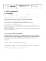
1. Introduction
This document explains how to install and run the graphical user interface of RTTOV. This interface
allows the user to modify an atmospheric profile, run RTTOV for a given instrument to produce the
radiances and brightness temperatures, and visualize the results instantly.
1.1. Installation
Using RTTOV GUI requires the following software to be installed :
- python2.7 (http://www.python.org/download/)
- wx python version 2.9.5 (http://www.wxpython.org)
- numpy (http://scipy.org/Download)
- matplotlib with backend_wxagg (http://matplotlib.org/)
- h5py version 2.0 or later (http://www.h5py.org/)
- HDF5 v1.8.8 or later (http://www.hdfgroup.org/HDF5/)
- RTTOV v11.3
The GUI also requires the f2py package to interface the Fortran and Python code. This is distributed
as part of Numpy v1.6 and later.
An easy way to install python 2.7 and all the python required packages is to use the anaconda
distribution of python proposed by continuum analytics http://continuum.io/downloads.
Anaconda already includes numpy, matplotlib and h5py and by default is installed on your home
directory. :
Add $HOME/anaconda/bin to your PATH :
$ export PATH=$HOME/anaconda/bin:$PATH
You can add this line to your ~/.profile (or ~/.bash_profile or similar).
Then, you just have to install the wxpython package with the conda command (which is part of
anaconda) :
$ conda install wxpython
The RTTOV GUI is provided as part of the RTTOV package in the gui/ directory.
Edit the file build/Makefile.local to point to your HDF5 installations (see section 5 of the RTTOV
user guide for more information about this).
Compile RTTOV with the rttov_compile.sh script : Change to the src/ directory and type:
$ ../build/rttov_compile.sh
3
A Graphical User Interface
for RTTOV v11.3
Doc ID
Version
Date
: NWPSAF-MF-UD-010
:2
: 2015 09 18
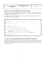
If your python installation is correct the script must see that f2py is present : answer “y” at the
question “...f2py detected: do you want to compile the Python wrapper and RTTOV GUI? (y/n)".
Be sure that the HDF5 library used for RTTOV is consistent with that used by h5py.
The rttov_gui_f2py.so symbolic link must point to the rttov_gui_f2py.so which is built in the
RTTOV lib/ directory.
RTTOV GUI needs profile files : hdf5 or ASCII files. ASCII files are actually python source code
files (see section 4 ).
ASCII and HDF5 versions of the RTTOV test suite profiles are included in the
rttov_test/profile-datasets-py and rttov_test/profile-datasets-hdf directories.
Update the rttov_gui.env environment file according to your installation (see next section).
Run the GUI :
$ source ./rttov_gui.env
$ ./rttovgui
If you use the emissivity and/or BRDF atlases with the GUI then note that you must use the HDF5
versions of the BRDF and IR emissivity atlas files.
2. RTTOV GUI User Manual
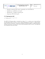
2.1. Configuration files
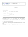
The rttov_gui.env contains mandatory environment variables which are used by RTTOV GUI.
This file must be customized to your specific installation. In most cases this only requires the
RTTOV_GUI_PREFIX variable to be specified with the absolute path to your RTTOV gui/
directory.
Example of rttov_gui.env file :
# RTTOV GUI Environment
#
# Mandatory variables :
# ------------------# RTTOV GUI installation directory
# absolute path to the rttov/gui directory e.g. /home/user/rttov11/gui
RTTOV_GUI_PREFIX=
export RTTOV_GUI_PREFIX
PATH=${RTTOV_GUI_PREFIX}:$PATH
export PATH
PYTHONPATH=${RTTOV_GUI_PREFIX}:${PYTHONPATH}
export PYTHONPATH
4
A Graphical User Interface
for RTTOV v11.3
Doc ID
Version
Date
: NWPSAF-MF-UD-010
:2
: 2015 09 18
# Optional environment variables : (the defaults are usually OK)
# -----------------------------# Directory for rttov emissivity and BRDF atlases: this should be the directory
# containing the emis_data/ and brdf_data/ directories which hold the atlas
# datasets. NB The HDF5 BRDF and IR emissivity atlas files must be used.
RTTOV_GUI_EMISS_DIR=${RTTOV_GUI_PREFIX}/../
export RTTOV_GUI_EMISS_DIR
# Working directory (for rttov gui temporary files)
RTTOV_GUI_WRK_DIR=$HOME/.rttov
export RTTOV_GUI_WRK_DIR
# Default directory for rttov coefficients files
RTTOV_GUI_COEFF_DIR=${RTTOV_GUI_PREFIX}/../rtcoef_rttov11
export RTTOV_GUI_COEFF_DIR
# Default directory for profile files
RTTOV_GUI_PROFILE_DIR=${RTTOV_GUI_PREFIX}/../rttov_test/profile-datasets-hdf
export RTTOV_GUI_PROFILE_DIR
2.2. Files created by the RTTOV GUI
The RTTOV GUI software will create various files in its working directory defined by the
RTTOV_GUI_WRK_DIR environment variable (~/.rttov by default.).
Most of these files are encoded in the HDF5 format. It is possible to look at them using the
hdfview software for instance. Exporting data to text file is also possible using the h5dump
command.
These files are :
•
profile.h5 : contains the profile and options.
•
surface.h5 : contains information about the surface and emissivity / reflectance used as input
and computed by RTTOV or modified by user.
•
radr.h5 : contains radiances computed by a run of RTTOV.
•
trns.h5 : contains transmittances computed by a run of RTTOV.
•
kmat.h5 : contains the K matrix computed by a run of RTTOV K
•
pc.h5 : contains the pcscores computed by a run of PC-RTTOV.
5
A Graphical User Interface
for RTTOV v11.3
Doc ID
Version
Date
: NWPSAF-MF-UD-010
:2
: 2015 09 18
•
pckmat.h5 :contains the K PC matrix computed by a run of PC-RTTOV K
•
tmpFileErr.log : last RTTOV error log file.
•
tmpFileOut.log : last RTTOV output log file
•
rttovgui.log : RTTOVGUI log file.
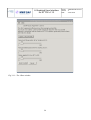
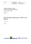
2.3. Starting the GUI
$ source ./rttov_gui.env
$ ./rttovgui
The RTTOV GUI main window is launched (see Figure 2.3.1) : it allows you to load coefficient
files (through the RTTOV menu), to open a profile (through the File menu), to modify options,
profile and surface parameters if necessary (through the dedicated windows available through the
Windows menu) and to run the RTTOV direct model (through the RTTOV menu). The application
log is displayed in this main window.
6
A Graphical User Interface
for RTTOV v11.3
Doc ID
Version
Date
: NWPSAF-MF-UD-010
:2
: 2015 09 18
Figure 2.3.1 : main window
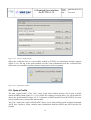
2.4. Loading RTTOV coefficient files
The first step is to choose an instrument you want to work with. For this purpose, you have to pick a
coefficient file using the RTTOV menu “Load coefficient” (figure 2.4.1).
You must choose a file by clicking on the Choose button.
An RTTOV coefficient file is always mandatory. If you want to work with aerosols you must
choose an aerosols coefficient file, and if you want to work with clouds, you must choose a cloud
coefficient file. All these files must be compatible (i.e. they must be for the same instrument and
contain coefficients for the same channel set).
Once your choices have been made, you can load the coefficient files by clicking on the “Load”
button, or by clicking on the “File” menu and selecting the “Load coefficient” menu item.
7
A Graphical User Interface
for RTTOV v11.3
Doc ID
Version
Date
: NWPSAF-MF-UD-010
:2
: 2015 09 18
Figure 2.4.1 : choose a coefficient file
When the coefficient files are successfully loaded by RTTOV an information window appears
(figure 2.4.2). The log in the main window provides some information from the coefficient files
such as the wave numbers and the reference temperatures of the instrument.
Figure 2.4.2 : information window
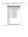
2.5. Open a Profile
The item “Open Profile” of the “File” menu of the main window permits you to open a profile
stored in HDF5 format (figure 2.5.1). If a profile file contains several profiles, you will be asked to
choose the profile number (figure 2.5.2). A selection of HDF5 profiles from the RTTOV test suite
can be found in rttov_tests/profile-datasets-hdf/.
The “File” menu item “Open ASCII Profile” allows you to read profiles stored in Python-formatted
ASCII files. Section 4 below contains more information about the HDF5 and ASCII profile file
formats.
8
A Graphical User Interface
for RTTOV v11.3
Figure 2.5.1 : select a profile
Figure 2.5.2 : choose a profile number
9
Doc ID
Version
Date
: NWPSAF-MF-UD-010
:2
: 2015 09 18
A Graphical User Interface
for RTTOV v11.3
Doc ID
Version
Date
: NWPSAF-MF-UD-010
:2
: 2015 09 18
2.6. Modifying the options
The RTTOV options can be modified through the Options editor window. Select “Options Editor
Window” from the “Windows” menu of the main window (fig 2.6.1).
The RTTOV options which can be modified are part of the option structure of RTTOV, described in
the RTTOV v11 User Guide (Annex O). The help menu of the Options editor windows gives you
some information. Some options are unavailable depending to the loaded coefficient files or the
profile content. For example, the “addclouds” option can only be checked if you have loaded a
cloud coefficient file. The “addaerosl” option can also only be checked if an aerosols coefficient file
is loaded. PC-RTTOV options can be modified only if you have loaded a PC RTTOV coefficient
file. Once you have made your choices you have to save them for the run by clicking the “Apply”
button.
10
A Graphical User Interface
for RTTOV v11.3
Figure 2.6.1 : Option Editor window
11
Doc ID
Version
Date
: NWPSAF-MF-UD-010
:2
: 2015 09 18
A Graphical User Interface
for RTTOV v11.3
Doc ID
Version
Date
: NWPSAF-MF-UD-010
:2
: 2015 09 18
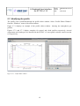
2.7. Modifying the profile
The profile can be modified through the profile editor window. Select “Profile Editor Window”
from the “Windows” menu of the main windows.
Figure 2.7.1 displays an example of the profile editor window showing the atmospheric gas
profiles.
Figures 2.7.2 and 2.7.3 display examples for aerosol and cloud profiles respectively. Aerosol
components and cloud types are described in the RTTOV v11 users guide section 8.6 and in section
8.5 respectively.
Figure 2.7.1 : Profile Editor window
12
A Graphical User Interface
for RTTOV v11.3
Figure 2.7.2 : Profile Editor window with aerosols
Figure 2.7.3 : Profile Editor window with clouds
13
Doc ID
Version
Date
: NWPSAF-MF-UD-010
:2
: 2015 09 18
A Graphical User Interface
for RTTOV v11.3
Doc ID
Version
Date
: NWPSAF-MF-UD-010
:2
: 2015 09 18
The left hand panel of the window shows the atmospheric components profiles grouped by type :
Gases, Aerosols and Clouds. The Temperature profile is always drawn on the three types of panel.
On the right hand panel of the window, the different components profiles are drawn separately. You
can modify the profile by hand by clicking in the panel. For that, select and visualize a component
profile on the right panel. Click the middle mouse button to modify the profile. The closest point on
a profile pressure level or layer is moved to the new value. The corresponding curve in the left
hand panel is also updated. In the right hand panel you can also click with the left mouse button and
drag a zone to zoom in. Click the right button to zoom out. Finally, apply your changes or save the
profile for the next run of RTTOV using the File menu.
14
A Graphical User Interface
for RTTOV v11.3
Doc ID
Version
Date
: NWPSAF-MF-UD-010
:2
: 2015 09 18
Edit menu options :
Undo : undo the last modification of the curve.
Redo : redo the last modification of the curve.
Insert : For aerosols or clouds only, clicking in the right hand panel moves or creates a new point.
Remove : For aerosols or clouds only, clicking in the right hand panel removes the nearest point
(sets the nearest layer concentration to zero).
Edit x axe : Change the X axis bounds.
Add gas : Add a gas.
Remove gas : Remove a gas.
Add aerosol : Add an aerosol particle type.
Remove aerosol : Remove an aerosol particle type.
Add cloud : Add a cloud particle type.
Remove cloud : Remove a cloud particle type.
Replace aerosol by clim : Replace all aerosol profiles with a climatological aerosol selection. The
user can choose between different types of climatology (see fig 2.7.4)
Figure 2.7.4 : Climatology choices for aerosols
15
A Graphical User Interface
for RTTOV v11.3
Doc ID
Version
Date
: NWPSAF-MF-UD-010
:2
: 2015 09 18
2.8. Editing the surface
The Surface Editor Windows allows you to modify the surface parameters of the profile. Select the
Surface Editor Window menu item from the windows menu of the main window.(Fig 2.8.1).
Figure 2.8.1 : Surface Editor Window
The File Menu of the Surface Editor Window allows you to load an atlas, or to modify the value of
emissivity or reflectance, channel by channel (Fig 2.8.2). After making changes you must select
“Apply changes” from the File menu.
The computed emissivity/reflectance values appear in red on the right hand panel. The input values
are in blue. If an atlas is loaded, the RTTOV model does not compute the emissivity or reflectance
values.
16
A Graphical User Interface
for RTTOV v11.3
Doc ID
Version
Date
: NWPSAF-MF-UD-010
:2
: 2015 09 18
Figure 2.8.2 : Edit Input Emissivity or BRDF Values. (Tip for check boxes : write 1 to check the box and 0 or nothing to
un-check the box)
17
A Graphical User Interface
for RTTOV v11.3
Doc ID
Version
Date
: NWPSAF-MF-UD-010
:2
: 2015 09 18
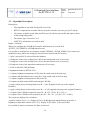
2.9. Running RTTOV Direct Model and working with the Radiance Frame
To run the direct model of RTTOV select “Run direct” from the RTTOV menu in the main GUI
window. This will save and overwrite the profile being edited and run the direct model (the profile
is saved before each run in the RTTOV GUI working directory: it does not overwrite the original
input profile file).
If the run is successful, a new window appears : the radiance window which displays the result of
the RTTOV direct model. (Fig 2.9.1)
Figure 2.9.1 : Radiance window
18
A Graphical User Interface
for RTTOV v11.3
Doc ID
Version
Date
: NWPSAF-MF-UD-010
:2
: 2015 09 18
The charts displayed in the radiance window are :
•
•
•
•
•
•
TOTAL : Clear+cloudy top of atmosphere radiance for given cloud top pressure and fraction
[mW/cm-1/ster/sq.m]
CLEAR : Clear sky top of atmosphere radiance (channels) [mW/cm-1/ster/sq.m]
BT : Brightness temperature equivalent to total radiance [Kelvin]
BT_CLEAR : Brightness temperature equivalent to clear radiance [Kelvin]
REFL : Reflectance calculated from total radiance [N/A]
REFL_CLEAR : Reflectance calculated from clear radiance [N/A]
It is possible to choose different types of visualisation :
byChannel : For each run, view of all charts with all channels values (fig 2.9.1)
In this view you can select :
• -- Run -- : to choose a run (needs at least 2 different runs)
• -- Pseudo Run -- : To see the difference between two successive runs (needs at least
2 different runs ) (fig 2.9.2)
byRun : For each channel, view of all charts with all runs values
In this view you can select :
• -- Channel -- : to choose a channel
• -- Pseudo Channel -- : for channel combinations
OnePlot : View of one chart (fig 2.9.3)
In this view you can select :
• The parameter : TOTAL BT REFL +CLEAR : choose a chart type
• -- Run -- : to choose a run
• -- Pseudo Run -- : difference between two successive runs
• -- Channel -- : to choose a channel
• -- Pseudo Channel -- : for channel combinations
19
A Graphical User Interface
for RTTOV v11.3
Figure 2.9.2 : Radiance window (by Channel view )
20
Doc ID
Version
Date
: NWPSAF-MF-UD-010
:2
: 2015 09 18
A Graphical User Interface
for RTTOV v11.3
Figure 2.9.3 : Radiance window (One Plot view run2-run1)
21
Doc ID
Version
Date
: NWPSAF-MF-UD-010
:2
: 2015 09 18
A Graphical User Interface
for RTTOV v11.3
Doc ID
Version
Date
: NWPSAF-MF-UD-010
:2
: 2015 09 18
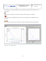
In the “byRun” view you may enter your own formula to compute a “pseudo channel”, for example
you can compute the difference between two channels, or more complicated formula. Your formula
will then appear in the “–Pseudo Channel –“ list. (fig 2.9.4)
Figure 2.9.4 : Radiance window (Compute a pseudo channel)
22
A Graphical User Interface
for RTTOV v11.3
Doc ID
Version
Date
: NWPSAF-MF-UD-010
:2
: 2015 09 18
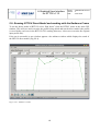
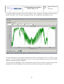
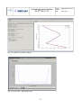
For high-resolution sounders such as IASI, AIRS or CrIS, a spectrum is displayed when the direct
model is run (fig. 2.9.5). For these instruments, the X axis is labelled in wavenumber (cm-1).
Figure 2.9.5 : Radiance window for hyperspectral instruments
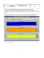
For any subsequent run you can select pseudo run such as “run 02 minus run 01” or “nun 02 versus
run 01” to see the spectrum differences (see fig. 2.9.6 spectrum difference between run 02 (with
addsolar) and run 01(without addsolar).
You must keep the Radiance Viewer window open between runs in order to compare results from
multiple runs. Once the Radiance Viewer window has been closed previous results are lost.
23
A Graphical User Interface
for RTTOV v11.3
Doc ID
Version
Date
: NWPSAF-MF-UD-010
:2
: 2015 09 18
Figure 2.9.6 : Radiance window for hyperspectral instruments : difference between 2 runs (with and without addsolar)
Instrument change or channel selection:
If you change the instrument by loading a new coefficient file, or if you select channels with the
“Select Channels” command of the RTTOV menu, the active radiance window which displays the
results of a previous RTTOV run will be closed by RTTOV-GUI.
Radiance window command line functionality :
It is also possible to launch the radiance window separately from the RTTOV GUI with the radr.h5
file containing the results of a RTTOV run (this file are kept by default in the $HOME/.rttov
directory) :
$ python rview/radianceframe.py radr.h5 [radr2.h5 ...]
Interactive navigation :
The toolbar at the bottom of the radiance window is the standard matplotlib tool bar : it allows you
to zoom and navigate the figure and save plots as image files.
24
A Graphical User Interface
for RTTOV v11.3
Doc ID
Version
Date
: NWPSAF-MF-UD-010
:2
: 2015 09 18
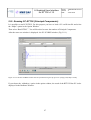
2.10. Running RTTOV K and working with the K-Matrix Frame
It is possible to run the K model of RTTOV. For this purpose, select the RTTOV menu from the
main window and then select “Run RTTOV K”. This will save and overwrite the profile and run the
K model.
If the run is successful, a new window appears : the K-Matrix Window which display the result of
the RTTOV K-Model (Fig 2.10.1). With every RTTOV K run, a new window is displayed.
Figure 2.10.1 : K-Matrix window
25
A Graphical User Interface
for RTTOV v11.3
Doc ID
Version
Date
: NWPSAF-MF-UD-010
:2
: 2015 09 18
Move the mouse on a channel and hit 'P' on your keyboard to display the K profile (Fig 2.10.2)
Icon toolbar :
You can also use the Kp icon to choose the channel of the K profile to be displayed.
This icon permits to multiply KProfile values by 10% of input profile; only applicable to gaz
variables.
If present these icons permit you to display the K matrix for different gases in the bottom plot.
Figure 2.10.2 : The K profile window
26
A Graphical User Interface
for RTTOV v11.3
Doc ID
Version
Date
: NWPSAF-MF-UD-010
:2
: 2015 09 18
2.11. Running PC-RTTOV (Principal Components)
It is possible to run PC-RTTOV. For this purpose you have to load a PC coefficient file and select
the “addpc” option in the Option Window.
Then select “Run RTTOV” . You will be asked to enter the number of Principal Components.
After the run a new window is displayed : the PC SCORES window (Fig 2.11.1).
Figure 2.11.1: The PC SCORES window. Note the symmetrical log axis for pcscores. (range [-100,100] is linear)
If you choose the “addradrec“ option in the option window, the result of the RTTOV Run PC is also
displayed in the Radiance Window.
27
A Graphical User Interface
for RTTOV v11.3
Doc ID
Version
Date
: NWPSAF-MF-UD-010
:2
: 2015 09 18
2.12. Running PC-RTTOV K
If you choose to run PC-RTTOV K , two windows are displayed : the KPCMatrix Window and the
KPC profile window.
The KPC profile window (Fig 2.12.1) allows you to visualize the KPC profiles. You can use the
sliders in order to modify the plot (first curve to be displayed and the number of curves displayed).
With every K PC run, new windows are displayed.
Fig 2.12.1 : The K PC profile window
2.13. Colour customisation
Matplotlib colours for the different windows can be customised : You can modify the
rview/colors.py file as your convenience in respect of the python syntax.
28
A Graphical User Interface
for RTTOV v11.3
Doc ID
Version
Date
: NWPSAF-MF-UD-010
:2
: 2015 09 18
3. 1Dvar functionalities
3.1. Introduction
There is a basic 1DVAR retrieval algorithm available with RTTOV-GUI. It uses the R-matrix and
B-matrix of the NWPSAF-1DVAR retrieval software ( see
https://nwpsaf.eu/deliverables/1dvar/index.html). In order to be independent from this software,
samples of these matrices are available in the RTTOV-GUI directory.
The basic 1DVAR algorithm can only be used for the following instruments :
"airs","iasi","amsua","amsub","mhs","hirs","atms","ssmis","cris"
The observation error R-matrix for iasi metop 2 and iasi metop 1 are identical.
Only one R-matrix for SSMIS is provided.
In order to have access to the 1Dvar functionalities, you have to open a 54 levels profile ( the
background error matrix are only available for 54 levels) and load the coefficients for one of the
previous listed instrument.
With these to prerequisites, you have access to the Configure 1Dvar command of the 1Dvar menu
of the main window (see fig 3.1.1)
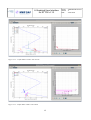
3.2. Running the RTTOV-GUI 1DVAR
RTTOV-GUI 1DVAR works with 2 profiles : a Background profile “Xb” and a True profile “Xt”
The Background Profile is opened in the main RTTOV-GUI window and can be modified as usual.
The True Profile is opened in the specific 1DVAR window (Fig 3.1.1) and cannot be modified.
If you change the coefficient file with RTTOV-GUI the 1DVAR window is reinitialized.
It is also possible to run the RTTOV-GUI 1DVAR basic algorithm without running the whole
RTTOV-GUI :
example :
$python rcontroller/r1dvarController.py \
-P=${RTTOV_GUI_PROFILE_DIR}/standard54lev_allgas.H5 \
-s=${RTTOV_GUI_COEFF_DIR}/rttov7pred54L/rtcoef_noaa_19_amsua.dat
The 1DVAR window is initialized in this case with the first profile of
${RTTOV_GUI_PROFILE_DIR}/standard54lev_allgas.H5.
29
A Graphical User Interface
for RTTOV v11.3
Fig 3.1.1 : The 1Dvar window
30
Doc ID
Version
Date
: NWPSAF-MF-UD-010
:2
: 2015 09 18
A Graphical User Interface
for RTTOV v11.3
Doc ID
Version
Date
: NWPSAF-MF-UD-010
:2
: 2015 09 18
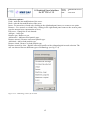
3.3. Algorithm Description
Restrictions :
•
This algorithm works with fixed profile levels (54)
•
RTTOV computations are made with no cloud,nor aerosols, nor trace gas (just T and Q)
•
All surface variables except Tskin and T2m are fixed for the true profile and equal to those
of the background profile.
•
The surface type is forced to “sea”
•
all RTTOV calculations are made at nadir
Inputs / selections :
When you configure the 1DVAR the R-matrix and B-matrix are read in the $
{RTTOV_GUI_PREFIX}/r1DVAR/data directory
It is possible to configure the environment variable NWPSAF_1DVAR_HOME if you want to use
another directory (but do not change the sub-directories names and file formats).
1. Open a true profile Xt selected from the database
2. Change the value of the scaling factor (fb) for the background errors if necessary
3. Change the value of the scaling factor (fr) for the observation errors if necessary
4. Change the value of the maximum random noise if necessary
5. Click on the RUN 1DVAR button
Computations made by RTTOV-GUI :
1. Compute brightness temperatures Y(Xt) from Xt (made only at the first step)
2. Compute and add random noise vector N to Y(Xt) (made only at the first step)
3. Compute brightness temperatures Y(Xb) from Xb
4. Compute jacobian matrix K(Xb) and transpose KT(Xb)
5. Apply scaling factor to background errors B --> fb x B (applied each step to the original
B-matrix)
6. Apply scaling factor to observation errors R --> fr x R (applied each step to the original R-matrix)
7. Compute linear 1DVAR weights W where W = B . KT . [ K .B . KT + R ](-1)
8. Compute linear 1DVAR retrieved profile (Xr) Xr = Xb + W . [ ( Y(Xt) + N ) - Y(Xb) ]
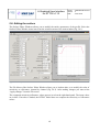
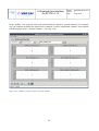
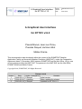
The results are displayed in 2 windows :
A profile window (Fig 3.2.1) : display the True, the Background and the Retrieved profiles; a
brightness temperature window (FIG.3.2.2) display Y(Xt)+Noise, Y(Xt) and Y(Xb).
It is possible to make a maximum of 9 Runs of retrieval.
31
A Graphical User Interface
for RTTOV v11.3
Fig 3.2.1 (Retrieved profile window)
Fig 3.2.2 (True BT – Background BT)
32
Doc ID
Version
Date
: NWPSAF-MF-UD-010
:2
: 2015 09 18
A Graphical User Interface
for RTTOV v11.3
Doc ID
Version
Date
: NWPSAF-MF-UD-010
:2
: 2015 09 18
By clicking the reset button : the 1DVAR window is reinitialized : the background profile is
reinitialized (if you a have made some changes on it with the surface window and/or the profile
window).
4. Input Profile file format
The input profiles for the RTTOV GUI can be of two different kind formats. The “native” profile
format is HDF5, as the Fortran executable GUI command will only read such format. The other
format is an ASCII format made of Python statements for the required variables. The two formats
are described below.
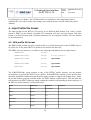
4.1. HD5 profile file format
The HDF5 profile format can store a single profile or a profile dataset such as the ECMWF diverse
83 profile set. It also allows RTTOV options to be stored in the same file.
The HDF5 top level structure is as follows (note all groups and datasets are in capital letters):
/PROFILES
Group
/PROFILES/0001
Group
First profile
/PROFILES/0002
Group
Optional
/PROFILES/9999
Group
Optional
/OPTIONS
Group
Optional
....
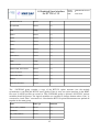
The /PROFILES/0001 group contains a copy of the RTTOV profile structure (see the module
src/main/rttov_type.F90 and RTTOV user's guide). If the HDF5 file contains several profiles they
should be numbered continuously and the group name is made of 4 digits with leading zeros. Under
the profile number group the variable names are HDF5 datasets (capital letters). The skin and s2m
sub-structures are HDF5 subgroups which contain the variables corresponding to those sub-types of
the RTTOV profile structure; see the table below.
Name
HDF5 type
Dimension
ID
Dataset
{SCALAR}
DATE
Dataset
{3}
TIME
Dataset
{3}
NLAYERS
Dataset
{1}
NLEVELS
Dataset
{1}
CTP
Dataset
{1}
33
Comment
A Graphical User Interface
for RTTOV v11.3
Doc ID
Version
Date
CFRACTION
Dataset
{1}
CLOUD
Dataset
{nlayers,6}
optional
CFRAC
Dataset
{nlayers}
optional
ICEDE
Dataset
{nlayers}
optional
IDG
Dataset
{1}
ISH
Dataset
{1}
CLW
: NWPSAF-MF-UD-010
:2
: 2015 09 18
optional, never used in GUI
AEROSOLS
Dataset
{nlayers,13}
P
Dataset
{nlevels}
T
Dataset
{nlevels}
Q
Dataset
{nlevels}
O3
Dataset
{nlevels}
optional
CO2
Dataset
{nlevels}
optional
N2O
Dataset
{nlevels}
optional
CO
Dataset
{nlevels}
optional
CH4
Dataset
{nlevels}
optional
BE
Dataset
{1}
COSBK
Dataset
{1}
SNOW_FRAC
Dataset
{1}
SOIL_MOISTURE
Dataset
{1}
LATITUDE
Dataset
{1}
LONGITUDE
Dataset
{1}
AZANGLE
Dataset
{1}
ZENANGLE
Dataset
{1}
SUNAZANGLE
Dataset
{1}
34
optional
A Graphical User Interface
for RTTOV v11.3
SUNZENANGLE
Dataset
{1}
ELEVATION
Dataset
{1}
S2M
Group
S2M/O
Dataset
{1}
S2M/P
Dataset
{1}
S2M/Q
Dataset
{1}
S2M/T
Dataset
{1}
S2M/U
Dataset
{1}
S2M/V
Dataset
{1}
S2M/WFETC
Dataset
{1}
SKIN
Group
SKIN/FASTEM
Dataset
{5}
SKIN/FOAM_FRACTION
Dataset
{1}
SKIN/SALINITY
Dataset
{1}
SKIN/SURFTYPE
Dataset
{1}
SKIN/T
Dataset
{1}
SKIN/WATERTYPE
Dataset
{1}
Doc ID
Version
Date
: NWPSAF-MF-UD-010
:2
: 2015 09 18
The /OPTIONS group contains a copy of the RTTOV option structure (see the module
src/main/rttov_type.F90 and RTTOV user's guide). There is only one option structure in the HDF5
file even if several profiles are stored in. This /OPTIONS group is optional. All RTTOV options
variables should be present. The logical variables are converted to integer datasets where “true” is
converted to 1 and “false” converted to 0. Note that the RTTOV options substructures are packed all
together in the same group.
Name
HDF5 type
Dimension
APPLY_REG_LIMITS
Dataset
{1}
VERBOSE
Dataset
{1}
DO_CHECKINPUT
Dataset
{1}
35
A Graphical User Interface
for RTTOV v11.3
ADDPC
Dataset
{1}
ADDRADREC
Dataset
{1}
IPCBND
Dataset
{1}
IPCREG
Dataset
{1}
ADDREFRAC
Dataset
{1}
SWITCHRAD
Dataset
{1}
USE_Q2M
Dataset
{1}
DO_LAMBERTIAN
Dataset
{1}
ADDSOLAR
Dataset
{1}
DO_NLTE_CORRECTION
Dataset
{1}
ADDAEROSL
Dataset
{1}
ADDCLOUDS
Dataset
{1}
USER_AER_OPT_PARAM
Dataset
{1}
USER_CLD_OPT_PARAM
Dataset
{1}
CLDSTR_THRESHOLD
Dataset
{1}
CLDSTR_SIMPLE
Dataset
{1}
OZONE_DATA
Dataset
{1}
CO2_DATA
Dataset
{1}
N2O_DATA
Dataset
{1}
CO_DATA
Dataset
{1}
CH4_DATA
Dataset
{1}
FASTEM_VERSION
Dataset
{1}
CLW_DATA
Dataset
{1}
SUPPLY_FOAM_FRACTION
Dataset
{1}
ADDINTERP
Dataset
{1}
36
Doc ID
Version
Date
: NWPSAF-MF-UD-010
:2
: 2015 09 18
A Graphical User Interface
for RTTOV v11.3
INTERP_MODE
Dataset
{1}
LGRADP
Dataset
{1}
REG_LIMIT_EXTRAP
Dataset
{1}
SPACETOP
Dataset
{1}
Doc ID
Version
Date
: NWPSAF-MF-UD-010
:2
: 2015 09 18
4.2. ASCII Text profile file
The RTTOV GUI is able to read an ASCII text profile file. This kind of file is made of Python
statements for the required variables. Thus the format should respect the Python language syntax.
The arrays should be defined as NumPy arrays, the scalars can be pure Python scalars or NumPy
variables.
The variable names are the ones described in the RTTOV users guide for the profile structure
(Annex O), capital letters; except for:
•
clouds where 2D cloud array is replaced by 1D cloud arrays, one for each cloud short name
(table 22 of users guide)
•
aerosols where 2D aerosols array is replaced by 1D aerosol arrays, one for each aerosol
short name (table 23 of users guide)
Units are as described in RTTOV users guide for profile structure (Annex O).
Pressure, temperature and water vapour arrays are mandatory; all other RTTOV profile variables are
optional, they will be set to default values when the profile is read.
The list of profile variables that can be set by the user is given below with the default values.
Omitted values default to a clear atmosphere. The number of levels and layers are deduced from
array sizes.
#" Mandatory arrays: P (hPa), T(K), Q(ppmv) on levels"
self["P"] = numpy.array([...])
self["T"] = numpy.array([...])
self["Q"] = numpy.array([...])
#"--------------------------------------------"
#" Optional profile variables "
#"--------------------------------------------"
#" Other Gases (ppmv on levels)"
self["O3"]
= numpy.array([...])
self["CO2"] = numpy.array([...])
37
A Graphical User Interface
for RTTOV v11.3
Doc ID
Version
Date
: NWPSAF-MF-UD-010
:2
: 2015 09 18
self["CH4"] = numpy.array([...])
self["CO"]
= numpy.array([...])
self["N2O"] = numpy.array([...])
#" Aerosols (1/cm3 on layers)"
self["INSO"] = numpy.array([...]) # Insoluble
self["WASO"] = numpy.array([...]) # Water soluble
self["SOOT"] = numpy.array([...]) # Soot
self["SSAM"] = numpy.array([...]) # Sea salt (acc mode)
self["SSCM"] = numpy.array([...]) # Sea salt (coa mode)
self["MINM"] = numpy.array([...]) # Mineral (nuc mode)
self["MIAM"] = numpy.array([...]) # Mineral (acc mode)
self["MICM"] = numpy.array([...]) # Mineral (coa mode)
self["MITR"] = numpy.array([...]) # Mineral transported
self["SUSO"] = numpy.array([...]) # Sulphated droplets
self["VOLA"] = numpy.array([...]) # OPAC Volcanic ash
self["VAPO"] = numpy.array([...]) # New Volcanic ash
self["ASDU"] = numpy.array([...]) # Asian dust
#" Clouds (g/m3 on layers)"
self["STCO"] = numpy.array([...]) # Stratus Continental
self["STMA"] = numpy.array([...]) # Stratus Maritime
self["CUCC"] = numpy.array([...]) # Cumulus Continental Clean
self["CUCP"] = numpy.array([...]) # Cumulus Continental Polluted
self["CUMA"] = numpy.array([...]) # Cumulus Maritime
self["CIRR"] = numpy.array([...]) # Cirrus
self["CFRAC"]= numpy.array([...]) # Cloud Fraction (should be set if any cloud)
self["IDG"]
= 1
# Scheme for Ice water content
self["ISH"]
= 1
# Ice cristal shape
#" Skin variables "
self["SKIN"]["T"]
= self["T"][-1]
self["SKIN"]["SURFTYPE"]
= 1
self["SKIN"]["WATERTYPE"] = 1
# (K)
# (0=Land, 1=Sea, 2=sea-ice)
#
(0=fresh water, 1=ocean water)
self["SKIN"]["SALINITY"]
= 37 # (%o)
self["SKIN"]["FASTEM"]
= numpy.array([0., 0., 0., 0., 0.]) # (5 parameters
38
A Graphical User Interface
for RTTOV v11.3
Doc ID
Version
Date
: NWPSAF-MF-UD-010
:2
: 2015 09 18
Land/sea-ice)
#" 2m and 10m air variables "
self["S2M"]["T"] = self["T"][-1] # (K)
self["S2M"]["Q"] = self["Q"][-1] # (ppmv)
self["S2M"]["P"] = self["P"][-1] #
self["S2M"]["U"] = 0 #
(m/s)
self["S2M"]["V"] = 0 #
(m/s)
self["S2M"]["WFETC"] = 100000 #
(hPa)
(m)
#" Simple cloud "
self["CTP"]
= 500.0 # (hPa)
self["CFRACTION"] = 0.0 # [0,1]
Clear sky is the default
#" Viewing geometry "
self["AZANGLE"]
= 0. # (deg)
self["ELEVATION"]
= 0. # (km)
self["LATITUDE"]
= 49.738
# (deg)
Lannion is 48.750,
-3.470
self["LONGITUDE"]
= -3.473
# (deg)
Exeter is
-3.476
self["SUNAZANGLE"]
= 0. # (deg)
50.726,
self["SUNZENANGLE"] = 0. # (deg)
self["ZENANGLE"]
= 0. # (deg)
self["SNOW_FRAC"]
= 0. # [0,1]
#" Magnetic field "
self["BE"]
= 0.3 # (Gauss)
self["COSBK"] = 1.
#" Mislaneous "
self["ID"]="This is my profile"
self["DATE"] = numpy.array([2014, 04, 30], dtype=int) # Year, Month, Day
self["TIME"] = numpy.array([12, 0, 0], dtype=int)
39
# Hour, Minute, Second
A Graphical User Interface
for RTTOV v11.3
Doc ID
Version
Date
: NWPSAF-MF-UD-010
:2
: 2015 09 18
4.3. How to create an HDF5 profile file from Fortran
RTTOV users can create an HDF5 profile file for use in the RTTOV GUI using the RTTOV
subroutine RTTOV_HDF_SAVE contained in src/hdf/rttov_hdf_mod.F90. This subroutine can write
any RTTOV structure to an HDF5 file.
For example a main Fortran program that can store a profile dataset and options in the same file
would contain the following statements:
Use hdf5
Use rttov_hdf_mod
Type(profile_type),
Pointer :: profiles(:)
=> NULL()
Type(rttov_options) :: opts
CALL OPEN_HDF( .TRUE., ERR )
!... statements that creates the profiles array
!... and statements that fills the options opts
CALL RTTOV_HDF_SAVE( ERR, "PROFILES.H5", '/PROFILES', &
CREATE=.true., PROFILES = profiles(1:nprofiles))
CALL RTTOV_HDF_SAVE( ERR, "PROFILES.H5", '/OPTIONS', CREATE=.false., &
OPTIONS = opts )
CALL CLOSE_HDF( ERR )
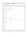
4.4. How to create an HDF5 profile file from ASCII text profile file
The ASCII text profile files are Python files. A Python script named convert_python2hdf.py in the
rttov_test/profile-datasets/ directory allows the user to convert an ASCII text profile to an HDF5
profile file. This script makes use of RTTOV GUI Python software (Profile class), so cannot be used
outside this framework.
40
A Graphical User Interface
for RTTOV v11.3
Doc ID
Version
Date
: NWPSAF-MF-UD-010
:2
: 2015 09 18
usage: convert_python2hdf5.py [-h] -i INPUTF [-o OUTPUTF]
[-g GROUP] [-v]
Import ASCII profile to HDF5 for RTTOV GUI
optional arguments:
-h, --help
show this help message and exit
-i INPUTF, --input-file INPUTF
input file name
-o OUTPUTF, --output-file OUTPUTF
output file name
-g GROUP, --group GROUP
internal HDF5 default is /PROFILES/0001/
-v, --verbose
display profile variables
It is possible to convert all of the RTTOV test suite profile datasets contained in
rttov_test/profile-datasets/ to ASCII and HDF5 format quite easily. Navigate to the
rttov_test/profile-datasets/ directory and then run:
$ ./run_convert_test2python.sh
$ ./run_convert_python2hdf5.sh
These scripts create profile-datasets-py/ and profile-datasets-hdf/ directories within rttov_test/
containing all of the RTTOV test suite profiles in Python ASCII and HDF5 formats for input to the
GUI.
Note that the second of these two scripts requires the gui/rttov/ directory to be in your
PYTHONPATH and rttov_gui_f2py.so must be linked in the profile-datasets/ directory.
41
A Graphical User Interface
for RTTOV v11.3
Doc ID
Version
Date
: NWPSAF-MF-UD-010
:2
: 2015 09 18
5. Reporting bugs and limitations
All main RTTOV GUI actions are logged in a file named "rttovgui.log" in the
RTTOV_GUI_WRK_DIR directory. If the user encounters an issue during the RTTOV GUI usage,
he should exit the program and copy the log file to a new name. This log file should be attached to
any request to the help-desk or forum. We encourage the users to share experiences through the
RTTOV forum at http://www.nwpsaf.eu/forum/
Restrictions:
– It is not possible to enter explicit cloud/aerosol optical parameters profiles for each channel.
– The RTTOV GUI is not compatible with RTTOV-SCATT.
Known bugs or current limitations:
– For the K calculations : only atmospheric gases, atmospheric temperature and TSkin
variables are displayed.
42