Download "user manual"

Rotor Wake/Stator Interaction Noise
Prediction Code
Technical Documentation and User's Manual
David A. Topol and Douglas C. Mathews
United Technologies Corporation
Pra tt & "Whitney
East H artfort!, CT
April 1993
Prepared for
Lewis Research Cen ter
Under Contract NAS3-25952 (Task 10)
NI\SJ\
National Aeronautics and
Space Administration
TABLE OF CONTENTS
Section ........................ : ...................................... , . . . . . . . .. Page
SUMMARY ....................................................................... 1
PART I: TECHNICAL DOCUMENTATION ........................................... 2
1. INTRODUCTION.............................................................. 2
2. P&WENHANCE1v1ENTSTOVOn ............................................... 3
3. PHYSICAL DISCUSSION OF PROGRAM CALCULATIONS ....................... 5
4. PROGRAM ASSUMP110NS . . . . . . . . . . . . . . . . . . . . . . . . . . . . . . . . . . . . . . . . . . . . . . . . . . .. 1D
5. PROGRAM INTEGRATION STATION CRITERIA. . . . . . . . . . . . . . . . . . . . . . . . . . . . . . .. 13
5.1 Chordwise Direction ....................................................... 13
5.2 Radial Direction. . . . . . . . . . . . . . . . . . . . . . . . . . . . . . . . . . . . . . . . . . . . . . . . . . . . . . . . . .. 1~
6. COMPUTATIONAL NOISE .................................................... 1&
7. CONCLUDING REMARKS ....................................................
2~
PART 2: USER'S MANUAL ........................................................ 21
1. INTRODUCTION ............................................................. 21
2. INPUT REQUIRE1v1ENTS ..................................................... . 22
2.1 General Namelist Input .................................................... .
2.2 Input Description ......................................................... .
2.2.1 Creating a Streamline Input .......................................... .
2.2.2 Standard Input Data Units ........................................... .
2.2.3 Case Descriptive Input Parameters .................................... .
2.2.4 Scalar Geometry and Performance Input ............................... .
2.2.5 Distributing the Streamlines in von .................................. .
2.2.6 Streamline Geometry and Performance Input ........................... .
2.2.7 Hub Vortex Parameters ............................................. .
2.2.8 Tip Vortex Parameters .............................................. .
2.2.9 Program Overiding Parameters ....................................... .
2.2.10 Developmental Parameters .......................................... .
2.2.11 Notes On Input .................................. , ................. .
21
21
21
24
24
25
26
26
2!
2~
29
29
3ij
-'
LIST OF ILLUSTRATIONS
Page
Figure
1
Sketch of V072 Rotor/Stator Geometry .................................. 5
2
Wake Model .......................................................... 6
3
WakeNortex Flowfield ................................................ 6
4
Cascade Unsteady Aerodynamics Geometry .............................. 7
5
Coupling the Unsteady Aerodynamics to the Noise ........................ 8
6
Powered Nacelle Geometry Vs. V072 Representation ..................... 10
7
Full Scale Engine Geometry Vs. V072 Representation ..................... 12
8
Wake Convection Along the Cascade ................................... 13
9
Radial Mode Shapes ................................................. 15
10
Wake TimelPhase Lag Due to Rotor Blade 1\vist ......................... 17
11
Radial Mode Shapes - Hub/Tip Ratio
12
Full Scale Engine Geometry Vs.
13
Definition of YRD and YSD .......................................... 27
14
Definition of XSD ................................................... 27
15
Tip Vortex Location, SBNT ........................................... 32
16
Flow Chart for the von Rotor Wake/Stator Interaction Program ........... 39
iii
= 0.38 ............................
19
von Representation .....................
23
SUMMARY
This report documents the improvements and enhancements made by Pratt & Whitney to two NASA
programs which together will calculate noise from a rotor wake/stator interaction. The code is a
combination of subroutines from two NASA programs with many new features added by Pratt &
Whitney. To do a calculation V072 first uses a semi-empirical wake prediction to calculate the rotor
wake characteristics at the stator leading edge. Results from the wake model are then automatically
input into a rotor wake/stator interaction analytical noise prediction routine which calculates inlet and
aft sound power levels for the blade-passage-frequency tones and their harmonics, along with the
complex radial mode amplitudes. The code allows for a noise calculation to be performed for a
compressor rotor wake/stator interaction, a fan wake/FEGV interaction, or a fan wake/core stator
interaction.
This report is split into two parts, the first part discusses the technical documentation of the program
as improved by Pratt & Whitney (P&W). The second part is a user's manual which describes how input
files are created and how the code is run.
1
PART 1: TECHNICAL DOCUMENTATION
1.
INTRODUCTION
In 1982 and 1984, two codes were developed: the GEIN ASA semi - empirical rotor wake/vortex model
(Ref. 1.) and the BBNINASA analytical rotor wake/stator interaction noise prediction computer
program (Ref. 2.). These codes together calculate noise in the duct from a rotor wake/stator
interaction. Pratt & Whitney under independent research and development funding has combined
and improved these codes. Additional improvements to the code's wake model were made under Task
10 of contract NAS3- 25952 along with the ability to run the code on a Silicon Graphics Workstation.
This section of the report documents the technical improvements to this new computer code (from
here on called V072 or the BBN/PW code). Documentation of the wake model improvements are not
discussed here but are instead discussed in the documentation of the above referenced contract.
The remainder of this part of the report is organized as follows. First there will be a brief discussion
of P& W program enhancements. From there, a physical discussion of how the new code works will
be introduced. The program assumptions will be introduced next including the rotor/core stator
interaction and duct assumptions. The program's P&W developed automatic radial and chordwise
integration station criteria used in calculations will then be presented. Lastly, calculation inaccuracies
due to program "computational noise" will be introduced so the user will be aware of where it is
important.
2
2.
P&W ENHANCEMENTS TO V072
A number of additions and improvements were made to the two NASA programs which now form
The resulting code has the following capabilities:
von since their receipt from NASA.
•
The program will now run:
The wake model by itself at any radii.
A compressor rotor wake/stator interaction or fan wakelFEGV interaction.
A fan wake/core stator interaction
Both a fan wakelFEGV intera;::tion and fan wake/core stator interaction.
•
Additional wake model capabilities:
Preliminary hub vortex model.
A tip vortex model.
A choice of three wake profiles: Gaussian or Hyperbolic Secant or Loaded
Rotor
A choice of two wake width and velocity deficit correlations: Original
GEfNASA correlation or the P&W high tip speed rotor correlation
• Multiple run capability (program input can be stacked).
•
Input is based on output from a 2D or axisymetric streamline-type, steady
aerodynamic prediction code.
•
Program criteria setting the number of spanwise and chordwise integration
points. This option my be replaced with user input integration station values.
These capabilities were achieved by initially combining the two NASA decks. In addition the program
was modified so that:
•
The code is no longer dependent on any external subroutines such as the matrix
inversion routine (except to obtain today's date).
User is notified of any program errors.
Program is now in double precision (necessary when working with small numbers
like acoustic pressures).
•
Bessel function subroutines were changed or replaced. The J - Bessel function
subroutine was replaced with one that is more reliable and calculates the
J - Bessel function and its derivative simultaneously. The Y - Bessel function
subroutine was changed so that it will calculate the Y - Bessel function and its
derivative simultaneously. These changes were intended to increase program
speed and accuracy.
3
•
The matrix inversion routine was changed from an IMSL routine to a routine
created by SIAM called UNPACK (Ref. 3.). This makes the code independent
of specific packages which my not be available on other computer systems.
The code will run on both Sun and Silicon Graphics Workstation platforms and
should be portable enough to run on other platforms.
The Loaded Rotor wake profile and and the P& W high tip speed rotor correlation were created using
Rotor 67 data under Task 10 of contract NAS3-25952. The details of how these items were created
is documented in a separate document.
4
3.
PHYSICAL DISCUSSION OF PROGRAM CALCULATIONS
The von program as originally received from NASA in the mid 1980's was designed by Eol t, Beranek
and Newman (Ref. 2.) to handle standard rotor wake/stator interactions in an infinitely long constant
area annular duct (Figure 1). Later, the wake model of Ref. 1. was added to the code to form the
present code. Discussions in this section will concentrate on how the program as updated by P&W
calculates noise from a rotor wake/stator interaction noise source. In Section 4. the method utilized
to set up the constant area duct will be covered. In addition, the extension of this procedure to include
rotor wake/core stator interactions will be discussed.
MEAN AXIAL VELOCITY
~
) The rotor 'lli2lf<e
c~{cu/,.:.:f'on
) ::Ji.L,.(O( nOise
Ie spell
se
C&(cu (c:.l,OI\
Figure 1
Sketch of V072 Rotor/Stator Geometry
The rotor wake/stator calculation is divided into two parts: the rotor wake calculation and the stator
noise response calculation. The performance input to this program will need to come from a two
dimensional or axisymetric streamline-type, steady aerodynamic prediction code. To expedite the
noise calculations the new program non -dimensionalizes all input geometry and performance. Then
before any calculations are done the program linearly interpolates the streamline
(radially-distributed) non-dimensional parameters to a "program-determined" number of
spanwise locations or "radial integration stations" (for the P&W developed criteria see section 1.2).
From there the program proceeds to the wake model calculation.
°e VO\--(O(
,cldlCI)
..<
To calculate the rotor wake, a program originally developed by General Electric under contract to
NASA was utilized (Ref. 1.). Essentially this program divides the annulus into streamlines (or strips).
It then unwraRs each strip to form a two dimensional flow in the circumferential and axial directions
(see Figure~).~No radial flow is E;rmitted:" A two-dimensional mean flow is calculated analytically
along each streamline with the assumption of incompressible flow across the rotor. This
incompressible flow assumption allows for the application of an analytical expression for the drag
coefficient which was utilized in creating the rotor wake empirical relationships used in the program.
A series of rotor wakes (combined with hub and tip vortices if desired) are then superimposed on the
mean flow to describe the flow field (see Figure 3). The streamwise wake widths and velocity deficits
are calculateq ~mpirically at the stator leading edge. The resulting wakes are then combined with hub
5
and tip vortices which are also calculated s~mi - empiri91~ at the stator leading edge. Details of these
calculations may be found in Reference 1.. Thus a combined wake/vortex profile is developed in rotor
fixed coordinates at the stator leading edge. A coordinate transformation to stator fixed coordinates
is then performed to calculate the flow uQwasl]....QY~~r to the mel!,n fl.9~\:Y direction in §.tator flxesL
coordinates. From these upwash velocity profiles, wake harmonic magnitudes and phases are
calculated at the stator leading edge for each harmonic at each radial strip location.
Ma
~
WAKE AT
'J.
flow
r=>
Pi ~ C9-' ('H~))
rll:
l
STATOR L.E.
;' ~ 1
ttl
V
I
PI
[:Y
INCOMING
FLOW
Figure 2
Wake Model
TIP VORTEX
FEGV
WAKES
FAN
HUB VORTEX
Figure 3
z)
WakelVortex Flowfield
At this point we arrive at the second part of the calculation: the calculation of~ue to the unsteady
flow l!fl~~QIl1h.~~~tQI£..For this calculation a programaeveloped by BOlt, Beranek, and Newman
(BBN) under contract to NASA (Ref. 2.) was used. Essentially this program calculates the total
harmonic power levels travelling forward and aft in the duct. To do this the program individually
calculates the circumferential/radial mode power levels for every propagating mode resulting from
this interaction. It then sums up all of the circumferential/radial mode power levels to obtain inlet
and aft total power levels for each harmonic. Two different sets of radial mode amplitudes and phases
are also calculated and output by the program. In the main output file the dimensional amplitude and
phase of the complex radial mode amplitudes normalized using the method outlined in Ref. 2. are
output. In a separate file, the real and imaginary parts of the dimensional complex radial mode
amplitude normalized as required by the Eversman Radiation Code (Ref. 4.) are output.
6
Originally the BBN/PW code had its own partial wake model which P&W replaced with the more
complete GE/NASA model. However, the wake "phase lag" (or wake skew) calculation in the original
code was retained to account for the greater distance that a wake at one radius must travel relative
to the distance that another wake must travel at another radius. This feature allows for the real effects
of wake/vane "slicing" to occur, rather than the simultaneous wake "slapping" limitation that was
imposed by earlier theories. In addition to the wake width and velocity deficit developed by General
Electric in Ref. 1, P&W has developed high tip speed wake width and velocity deficit correlations
under NASA Lewis funding. Also a skewed loaded wake profile based on Rotor 67 high tip speed wake
data (Ref. 5.) was developed. These additions to the wake model are included in the present code.
The development of these correlations are discussed in a separate document.
Given this unsteady wakelvortex flow we must now calculate the unsteady chordwise pressure
distributions on the vanes along the stator span. This type of calculation has been developed by a
number of authors including Verdon (Ref. 6.), Whitehead (Ref. 7.) and Smith (Ref. 8.). Verdon's case
is the most recent in which he developed a two dimensional cascade calculation which includes real
cascade geometries and steady as well as unsteady lift. Whitehead and Smith are older but are more
like what the program utilizes. In both of these cases the authors assume two dimensional
compressible flow over a cascade of unloaded flat plates at zero incidence to the incoming flow (see
Figure 4). In each case the annulus of vanes was unwrapped to form an infinite cascade along each
streamline (or strip). For this rotor wake/stator interaction program a procedure outlined by
Goldstein (Ref. 9.) utilizing the same assumptions as Smith and Whitehead was employed so that
according to Ventres (Ref. 2) all three formulations give the same results.
I
I
--:cJ
i 1 f t j : : R E DISTRIBUTION
GEOMETRY IS DEFINED FOR EACH STREAMUNE (OR STRIP)
w
=
Upwash Velocity
u
=
Freestream Absolute Velocity
OcH
=
Vane Stagger Angle, Ochord
Figure 4
Cascade Unsteady Aerodynamics Geometry
The program extends the strips formed during the wake calculation along the stator cascade and
proceeds to calculate unsteady pressure distributions on a reference vane of the cascade at a
program-specified number of chordwise stations (for the P&W developed criteria see section 1.1).
The program assumes that all the vanes in the cascade are of the same geometry and are equally
spaced in the circumferential direction.
7
At this point the program rewraps the strips to re-form an annular duct. We now have chordwise
pressure distributions along the span of a reference vane in an annular duct. Pressure distributions
on the other vanes may be calculated knowing the phase relationships that are a function of the blade
and vane number. Physically we can say that we now have an annular duct which contains chordwise
pressure distributions along every stator in the cascade and across the vane span (see Figure 5).
A
r--l
I
I
I
I
I
I
I
I
I
I
• •
STATOR
-
CALCULATE POWER LEVELS ALONG SEcn ON A·A
-
DENOTE PRESSURE DI STRI BUTJON POI NTS BY'.'
-
EACH· IS COUPLEDTO EACH RADIAL MODE USNGADUCT ACOUSTICMETHOO
(GREENE'S FUNCnON)ANO IS COMBI NED ATSECTJON A·A
-
THI S FORMS THE DUCT Acousn C PRESSURE FIELD
FOR EACH RAOI AL MODE AT SEcn ON A·A
LOOKING AFT
PRESSURE DI STRI BUTI ONS
ON EVERYVANE INTHE DUCT
Figure 5
Coupling the Unsteady Aerodynamics to the Noise
Assuming a mean axial flow in a constant area annular duct we can now calculate the radial mode
amplitudes for each propagating circumferential/radial mode. To understand this calculation we can
look at an axial location, A - A, in Figure 5. At this location we can evaluate the effect of the unsteady
pressures propagating from the cascade and then sum up these effects to calculate the amplitude of
each propagating mode in the duct (termed the Greene's function approach outlined in Ref. 2. or Ref.
9.). The calculation is done preserving all magnitudes and phases of every pressure in the pressure
distributions including how those pressures couple to each circumferential and radial mode. These
pressures are then integrated for each mode thus giving us an inlet and aft power level and complex
radial mode amplitude for each propagating mode. This process is repeated for every propagating
mode and the power levels are then summed up to give the circumferential mode power levels and
total power levels for each harmonic.
8
It should be noted that these noise calculations give inlet and aft mode amplitudes, phases and power
levels which are at an axial location associated with the stator hub leading edge (section A-A in Figure
5). Thus this axial location should be used as a starting point for propagating the modes upstream and
downstream in the duct. Further details of this method may be found in Reference 2 ..
9
4.
PROGRAM ASSUMPTIONS
The previous section physically discussed the program assumptions and calculation procedures for a
rotor wake/stator interaction occurring in a constant area duct (Figure 1). Real life configurations of
concern are, however, somewhat more complicated than this geometry. The real duct configurations
of interest include the following applications:
1. Compressor rotor wake/stator interactions,
2. Fan wake/FEGV interactions,
3. Fan wake/core stator interactions.
To calculate noise using von it is necessary to simplify the real duct geometry by making some
reasonable assumptions. To best visualize the problem let us look at the rotor wake/stator interaction
configuration of Figure 6. Figure 6a shows the Pratt & Whitney Powered Nacelle (APN) fan rig
geometry while Figure 6b illustrates how the APN geometry is represented in von using a constant
area duct.
BLADES
VANES
(a) Powered Nacelle Geometry
BLADES
VANES
(b) von Powered Nacelle Geometry
Figure 6
M44468·3
920608
Powered Nacelle Geometry Vs. V072 Representation
To choose a constant area duct we must consider its effect on the modal content of the noise, and its
influence on the rotor wake and stator pressure distribution calculations. The effect of the choice of
duct radii on the wake calculation occurs in the computation of the drag coefficient (to obtain wake
width and velocity deficit) and in the computation of the tip vortex. In the pressure distribution the
choice of duct radii effects the calculation of vane solidities and certain streamline performance such
as wheel speeds. The noise propagation calculation is influenced by radius in the calculation of the
cutoff ratio which sets the number of propagating modes and calculates mode dipole alignment.
10
Therefore, the chosen location for the constant area annular duct should occur near the stator where
the noise is generated but not far from the rotor where the wake is generated and where the wheel
speed is set. As a result the rotor leading edge is recommended for most configurations unless the
change in radii from the rotor to the stator is very large. It should be noted, however, that all geometry
and performance at the rotor leading edge and downstream should be selected along the streamlines
starting at the rotor leading edge. The method for creating the input to the code using this method
may be found in Part 2 of this document, the program user's manual.
What do these assumptions mean? Effectively what we have done is to choose streamlines at radii
at the rotor leading edge. We have then followed those streamlines to the stator using the geometry
and performance along each streamline with the exception of the effects of changing radii. We then
effectively treat the streamline like a string which goes from the rotor leading edge to the stator trailing
edge with geometry and performance (except the radii) which vary according to the real streamline
geometry. We can think of this string as being pulled taught to form streamlines in our constant area
duct in Figure 6b.
Now consider the more complicated case of a real fan stage like that shown in Figure 7a. The
simplification of this configuration is shown in Figure 7b. To obtain to Figure 7b from Figure 7a we
made a number of reasonable assumptions. First, as we concluded in the rotor wake/stator interaction
case discussed above the rotor leading edge radii could be used. In the case of the fan wake/FEGV
interaction, FEGV's are usually far enough back from the splitter so that the propagation or decay
of modes from this noise source will occur in the fan bypass duct. Therefore the rotor leading edge
radii are chosen for this interaction from the splitter streamline to the tip streamline with all modes
propagating in the fan bypass duct.
For the rotor wake/core stator interaction many more assumptions are needed. If the core stator
leading edge is less than a wavelength (at 3BPF) from the splitter leading edge, then we can reasonably
assume that decay will not be significant in the inner duct forward of the core stator and that all noise
propagation and decay will occur in the fan inlet duct. Thus the fan inlet duct is the core stator's
"constant area duct." However, no noise may propagate radially through the splitter until the stator
leading edge. Consequently, while only noise will be generated on the core stator itself we must
effectively extend the core stator across the entire inlet duct (see Figure 7b). An effect of these
assumptions is that any wave reflections off the splitter leading edge at the entrance to the primary
duct are neglected. In addition, these assumptions have effectively removed the splitter from the
problem.
The application of these assumptions to the computer program input can now be explained. For the
fan wake/core stator interaction there is no wake impinging on the core stator extension shown in
Figure 7. Thus in applying the above assumptions the programneed only integrate across the real core
stator. As will be found in Part 2 of this document, only streamlines for flow through the core stator
need to be specified in the program. Then to create the fan inlet duct the program will ask for the fan
outer diameter. Therefore the core stator duct has been created.
In applying these assumptions to the fan wake/FEGV interaction, only streamlines associated with
the fan bypass duct need be specified. This, plus the fan outer diameter (which will be the same as
the radius of the most outer streamline) will form the constant diameter duct.
When doing both predictions simultaneously the splitter diameter is simply input twice at the point
where the fan/core stator interaction input ends and the fan/FEGV interaction input begins. Then
both ducts will be automatically specified. See Part 2 of this document for more information on the
mechanics of the input.
11
As a result we have defined our constant area ducts for all three configurations of interest.
FAN
(a) Full Scale Engine Geometry
~
J
FAN
I!\ILET
DUCT
-I
I
I
I
I
I
I
SPLrrTER-
STREAMLINE
l
PRMARY
DUCT
I
I
I
I
FAN BYPASS
i
DUCT
I
I
I
I
FAN
(b)
Figure 7
~CORE
STATOR
'l
FEGV
CORE STATOR EXTENSION USED
IN FAN/CORE STATOR INTERACIDN
von Full Scale Engine Geometry
Full Scale Engine Geometry Vs. V072 Representation
12
5.
PROGRAM INTEGRATION STATION CRITERIA
As was discussed earlier the program chooses how many points it needs along the stator span and
stator chord to effectively calculate the total power levels. The program as received from NASA
lacked this capability. Consequently, it was necessary to create these criteria. In each case we need
to ask how rapidly in space the important parameters relating to the noise will change in the spanwise
and chordwise direction. These criteria were developed based on a total power level accuracy of plus
or minus IdB.
5.1 CHORDWISE DIRECTION
Let us first look in the chordwise direction. As the rotor wakes reach the stator they cause an upwash
to convect along the stator (Figure 8). This upwash varies along the chord causing an unsteady
pressure distribution to form along the chord (Figure 8a). As the wake continues travelling down the
stator chord another wake reaches the stator at a later time (Figure 8b). This wake will cause an
upwash velocity at an upstream location on the chord while the earlier wake is disturbing a
downstream section. In our case we are looking at a specific harmonic of the wake so that the wake
disturbance on the chord will be a sinusoidal shape. For BPF this sine wave will have as many cycles
on the vane as there are wakes on the vane; for 2BPF there will be twice as many, for 3BPF three times
as many, etc. In other words, the more variations we have on the chord at once, the more points we
will need to accurately calculate the chordwise pressure distribution on the vanes, and to later
integrate these chordwise pressures during the duct noise calculation.
W
FLOW
DIRECTION
SECONDWAKE
_ ~ WAKE CONVECTION FROM FIRST WAKE
\
CAUSES UNSTEADY PRESSURE
..!,LONG THI S REGION OF THE CHORD
t- .'.
,
-
-
-
-
~ FIRST WAKE DSTURBANCE
w~
_
SECONDWAKE DSTURBANCE
-
-
M44468-7
920608
Figure 8
Wake Convection Along the Cascade
13
n
C")c<~
v','
I
/1'
The criteria which was formed to represent this variation is:
NCHORD == 2 x PI x (Number of convected disturbances on the vane)
where NCHORD == number of points on the chord at which unsteady pressures are calculated.
This criteria is found to be equivalent to setting NCHORD equal to two times the reduced frequency
of the convected wakes in the chordwise direction.
e . g. NCHORD
=
2 x (Reduced
Frequency)
=2 x
(
2m1BNlb)
60U
where: n
B
Nl
U
b
= BPF harmonic,
= Number of Rotor Blades,
Z!f rC;f~ :~'.
= Fan rotational speed (revolutions/sec),
= flow velocity in stator fixed coordinates (ft/sec),
= 112 stator aerodynamic chord (ft).
Because the program Simpson's rule integration requires an even number of data points this criteria
is then raised to the nearest even number. To insure reasonable accuracy at low reduced frequencies
a minimum value of 8 is used. To increase program running efficiency a different NCHORD value
is utilizt:d for each wake BPF harmonic. In addition, the maximum NCHORD value is set to 60.
5.2 RADIAL DIRECTION
Obtaining a radial integration station criteria was found to be significantly more involved than the
chordwise case. 1\\10 parameters are important in this case. The first one relates to the number of
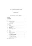
zero crossings a radial mode shape makes across the span. An example of this is shown in Figure 9
for the (4,0) and the (4,21) modes. We know that the radial mode shape of the (4,0) mode has no zero
crossings while the radial mode shape of the (4,21) mode has 21 sign changes along the span. As can
be seen the number of radial stations needed to effectively represent the (4,21) mode shape is going
to be many more than are needed to represent the (4,0) mode shape. The problem then becomes one
in which we cannot efficiently calculate which modes will be cuton and cutoff before we enter the
program for every circumferential and radial mode and effectively use this information. However we
can do this calculation for one mode per harmonic: i.e. the m = 0 mode, which if generated would have
the highest number of propagating radial modes. Since we can calculate how many radial modes will
propagate from this circumferential mode for each harmonic then we can efficiently utilize this
information to choose a conservative estimate for the number of radial integration stations we need.
Consequently, it was determined that we need at least two points along the span (i.~. the hub and the
tip points) plus two more points for every time the radial mode shape crosses zero. In addition, the
specialized integration procedure in the program requires an odd number of radial integration points.
As a result the criteria becomes:
NRADI
=
=
=
where: NRADI
MU
=
=
2(MU+1) + 1
2 x (No. of radial mode zero crossings) + 2 + 1
2xMU+3
Number of Radial strips required based on acoustic radial mode shape.
Highest order radial mode which propagates at a given BPF harmonic for an
m = 0 circumferential mode (Also equal to the number of radial mode zero
crossings).
14
N
+-------------------------------------~~----------~
w
Oro
~ .+-------------------------~------------------------~
f-O
-I
0..
::2'
<{
'<t
o
+---------~~--------------------------------------~
o
O+-__~----~----~--~----~----~--~----~----~--~
HUB
TIP
RADIUS
(a) (4,0) Mode
f\
A
~
A
~
"
1\
1\
"
"
I
w
°
~O
f-
-I
0..
~
<{
I
N
'J
V
\J
V
V
\.J
V
V
V
lJ
I
HUB
TIP
RADIUS
(b) (4,21) Mode
Figure 9
Radial Mode Shapes
15
The second parameter we need to consider relates to the number of wakes "slicing" along the stator
span at anyone time. To best explain this aspect we consider Figure 10 which illustrates the
rotor/stator geometry relative to the wake flow geometry. To obtain maximum aerodynamic
efficiency, standard high bypass ratio fans are highly twisted along the span. This twist from hub to
tip causes the wakes at the tip to travel further than the wakes at the hub (Figure lOa). The result is
that the circumferential locations of the wakes from hub to tip create a line which is highly canted
where the cant angle increases as the wakes travel downstream. Consequently, at anyone time the
stator may experience more than one rotor wake on its span at once (Figure lOb) resulting in pressure
variations along the span. At anyone time on a high bypass ratio engine there may be up to four
spanwise wake variations along the span. These variations are handled in terms of harmonics in much
the same fashion as the chordwise variations where the number of pressure variations increases with
each higher harmonic (Le. if there are four actual wakes in contact with a given vane, then at 3BPF
there will be 12 spanwise phase variations in upwash velocity).
Thus, a parameter called the wake phase lag is used to set the number of radial variations. The phase
lag is a form of reduced frequency which has the form:
NRAD2
=
=
2 x PI x (No. of spanwise wake disturbances on the stator span)
Wake Phase lag relative to the hub.
The required number of radial integration stations is now calculated by simply choosing the highest
calculatt:d value from the two NRAD criteria (either NRADl or NRAD2)' To insure reasonable
accuracy, minimum values have been set based on the type of run. For a rotor wake/stator interaction
without any vortices NRAD must be at least 11. To insure reasonably accurate vortex representation
the minimum is raised to 21 when a vortex is calculated. This is done to deal with the evenly spaced
radial integration stations utilized by the program. Due to the program's structure one NRAD value
is then employed corresponding to the highest harmonic being calculated.
To calculate NRAD for the rotor wake/core stator interaction a variation on this criteria was
introduced. As was suggested before, the core stator only generates noise along its real span (see
Section 4. and Figure 7). Therefore we need only integrate along the core stator span itself, i.e. we
need not integrate over the entire inlet duct. So to determine NRAD for this case we simply take the
value calculated for the total inlet duct and multiply it by the percentage of the total span which is
occupied by the core stator. This criteria significantly reduces computational time without affecting
program accuracy. For this case the minimum NRAD value is set to 7. The present maximum for
NRAD is set at 79.
After formulating these criteria a battery of test runs were initiated using the APN and full-scale
engine data input. Results indicated that the criteria were effective in giving accurate results.
16
ROTORT.E.
L.E.
- - - t > X - - - - I . . - - ~STATORL.E.
HUB WAKE TRAJECTORY
t>X= ROTOR TO STATOR
AXIAL SPACING
r41
c
CIRCUMFERENTIAL
DISTANCE BETWEEN
THE TWO WAKES
ATSTATORL.E.
TIP WAKE TRAJECTORY
(a) Cascade View
(b) End View of Wakes at Stator Leading Edge
Figure 10
Wake T/.l1le/Phase Lag Due to Rotor Blade Twist
17
M44468·2
920608
6.
"COMPUTATIONAL NOISE"
In numerical analysis applications such as this program the potential exists for the computer to add
noise of its own due to computer roundoff or truncation error. This is particularly true in the BBN/PW
code for a rotor wake/core stator interaction. This is because many mode shapes concentrate
themselves at the tip where the noise generated at the core stator is not a factor. To minimize this
problem the program has been designed to detect very small numbers in the J - Bessel function
subroutine so as to minimize computational noise. However, even with this improvement some
computational noise is likely to occur when the J - Bessel function goes to zero. This computational
noise is normally worse when the calculation of the critical mach number also does not converge (see
Part 2, Section 4). The improvements made to the code have rendered computational noise
insignificant for the FanlFEGV interaction noise predictions and most Fan/core stator noise
predictions. However, it does have an effect on Fan/core stator predictions where the expected noise
is relatively low.
There are sometimes instances where judgement is required to ascertain if the generated noise for
a particular radial mode is actually due to computational noise. An example of this occurs in a full
scale engine (for example Figure 11) where a rotor wake/core stator interaction generates the m~38
mode. Figure 11 illustrates the (38,0) and (38,1) modes as they are generated in the present code.
In this situation the expected power levels for BPF for these modes are near zero dB. However. real
predictions give power levels at BPF for these modes are 14dB and 81dB respectively. Note that the
associated Fan/FEGV noise prediction for this case is much higher (closer to 120dB) and is not
effected by computational noise. Both of the rotor/core stator answers, however. are due to
computational noise.
Figure 11 a shows the actual mode shapes. These mode shapes look quite correct with the mode shapes
having zero value across part or all of the core stator span and a zero slope at the hub and ti p. However.
we need to look at the mode shape in the region where the core stator is located (Figure 11b). In
Figure 11b it is seen that the (38,0) mode still is near zero accounting for the 14dB power level result.
In the (38,1) mode case there is a "tail" near the hub which is not in fact at zero slope to the hub with
error showing up in the third decimal place of the radial mode shape. This tail is due to the fact that
both J - Bessel function and its derivative go to zero while the Y - Bessel function goes to minus
infinity. The Bessel function calculation develops errors in calculating these results correctly and thus
a "tail" develops in the results in the hub region. This 81dB result is representative of a worst case
scenerio using the improved J - Bessel Function subroutine. The routine originally supplied with the
BBN code (Ref. 2.) allowed computational noise at the core stator to rise as high as 120dB which is
unacceptable when the real noise is at this level.
This type of problem shows up for high circumferential mode lobe numbers with low radial mode
orders and is at its worst when a "critical mach number not converged" warning is seen in the printout.
When this occurs the rotor wake/core stator results should be suspect for that mode and a radial mode
plot should be made to check the results.
While these numbers add no noise to the total result they do mislead the user into incorrectly
concluding that some tone noise was generated by this mode when in fact there was none.
18
n,---------------------------------------------------,
N+-------~--------,f----1/
''/
/
(38,1)MO~:A,L
w
/
o
::J
,.. ,-----... .......
t-
~{
<:
1'-/"
----.,.,..
,,,/
\
~
./
"
'\
\
(38,0) MODE
,
\
,
\
\,
./
/
/
\
I
\"
/
I
N
I
I
I+---~----~----~--~----~--~----~----~------~
HUB
TIP
RADIUS
I
CORE
I
j"4-STATOR ~
I
I
\
\
~
(a) Mode Shapes
no
I
.
0':"
..
~
...........
. ..
,
..
.
.,
\,
COMPUTAnONAL ERROR
,
\
\
(38,1) MODE
\j
.. . .
/
',""
,
,
,
, ----
''',-- ,,'
-----.
.
.
.
.
----- .. ...----
- ......
(38,0) MODE
Lfl
o
I
o
HUB
SPLITTER
RADIUS
(b) Enlargement of Core Stator Region
Figure 11
Radial Mode Shapes - Hub/TIp Ratio = 0.38
19
7.
CONCLUDING REMARKS
Two NASA computer codes were combined and improved to form a new rotor wake/stator interaction
code. Program capabilities include the ability to run noise predictions from the following noise
sources:
Rotor wake/stator interaction (in a low pressure compressor stage),
•
Fan wake/core stator interaction,
•
Fan wakelFEGV interaction (in a fan stage).
A semi - empirical tip vortex calculation and a partial hub vortex calculation are also available.
Finally, under certain circumstances the program will insert computational errors of its own giving rise
to computational noise. Thus when running rotor wake/core stator interaction noise predictions, care
should be taken to check mode power levels for this effect.
20
!Q
PART 2: USER'S MANUAL
1.
INTRODUCTION
The BBN/PW code has been designed to calculate noise from the following sources:
•
Compressor rotor wake/stator interaction.
•
Fan wakelFEGV interaction.
•
Fan wake/core stator interaction.
If desired, the program will also run the wake/vortex flow calculation. A tip vortex or preliminary hub
vortex calculation may be run with the wake prediction.
Part 2 of this document discusses what is required to run this program including all program
enhancements to date.
The program may be run in the workstation environment. About 10 minutes of time is needed to run
a noise prediction on a Sun SPARe 2 Workstation for an average engine condition. However, a
prediction of the only the wake runs eXtremely quickly. The namelist input is used in this program
where multiple cases may be run by simply stacking one namelist input above another. The code
presently requires geometry and performance parameters as a function of radius accross the fan,
FEGY, and core stator (if applicable).
21
2.
INPUT REQUIREMENTS
The Rotor Wake / Stator Interaction Program uses Namelist input. It gives flexibility to the user in
entering the data. It does not require all possible input be in the data file. Variables can be left out of
the input file with ease. Thus minimal input from the user is required.
2.1 GENERAL NAMELIST INPUT
The following is a general description of how the input file for
von is set up :
Title - this can be up to 80 characters in length and is the title for the case being run. If a title isgoing
to be entered it must be input before the Namelist data. If no title is entered the program will use a
default title based on the case being run.
The namelist data section of the input file is to be set up as follows:
Column 1 of each record must be blank.
All data must start in column 2
The first record of a namelist set of data must contain &INPUf The data may be entered starting on
the same line as the &INPUT or on the next line. If it is to be entered on the same line as the &INPUT
a blank space must separate the data from the &INPUI
The data is to be entered separated by commas. As much data as fits can be entered on a single line
and the order of the variables is irrelevant.
The form of the data is VARIABLE NAME = DATA VALVE or, ARRAY NAME = DATA
VALVES (Each element separated by a comma)., The last record of a set of data must contain &END
Multiple cases can be input in the same data file. This is set up as if the cases were in separate files.
Each case needs its own namelist input. Only those items that need to change from the previous case
must be defined in the new namelist set. Once each case is defined they can be stacked on top of each
other in the file. For more information regarding the set upofthe input data file refer to the Appendix
(Sample Input).
2.2 INPUT DESCRIPTION
2.2.1 Creating a Streamline Input
To obtain input to von we need to first transform our real engine geometry (Fig. 12a) into a constant
area duct geometry (Fig. 12b). To obtain Figure 12b from Figure 12a, visualize each streamline like
a "string" with geometry and performance varying along the "string." Now pull the string so it is taught
where the radius of the string from the engine centerline corresponds to the rotor leading edge radius
of this streamline.
Thus, each streamline is located at the rotor leading edge radius to create the constant area duct. We
then follow along each streamline back to the stator to obtain engine geometry and performance
parameters.
22
For example:
Looking at Figure 12, streamline 2: to get from Figure 12a to 12b look at the streamline radius at pain t
A in Figure 12a. This radius will be the radius of the streamline in the program. Therefore utilize
geometry and performance at points A,B,C. Identify the rotor chord along point A to B and the stator
chord from point C to D respectively (this is the aerodynamic chord). Do not use the axial chord. Use
the aerodynamic chord as defined on a streamline. Use the stator stagger angle at an airfoil
cross-section starting at point C. Identify the axial spacing as the streamline distance from points B
to C.
STREAMLINE 1 ' ••
STATOR
A
STREAMLNE 2 ...............
--
B________ C
FAN
(a) Full Scale Engine Geometry
STREAMLNE 1
A ___ ~
9 9__ .
PRfv1ARY
DUCT
'.....
CORE"\.
STATOR
STREAMLNE 2 ____A
_ _ B________
p ___ 0
FANSVPASS
DUCT
FEGV
FAN
(b) V072 Full Scale Engine Geometry
Figure 12
Full Scale Engine Geometry Vs. V072 Representation
23
For more information on the choice of radial locations see Section 4. of Part 1 of this document. Note
that if the radial change on the engine from the rotor leading edge to the stator leading edge is
significant a program streamline radial location other than the rotor leading edge may be desirable.
2.2.2 Standard Input Data Units
Standard Input Data Units
•
Lengths - - - Inches
•
Rotor speed - - - RPM
•
Temperatures - - - Degrees Rankin
•
Densities - - - Ibm/ft 3
•
Angles - - - Degrees
All air and stagger angles are defined relative to the circumferential direction.
2.2.3 Case Descriptive Input Parameters
IPRED - type of prediction
= a Compressor rotor wake prediction only
= 1 Rotor/Stator or FanIFEGV interaction only (default)
= 2 Fan/Core stator interaction only
= 3 Both Fan/FEGV and Fan/Core stator interactions
NDATS
No. of streamlines where streamline information will be input for a rotor/stator or
rotor/FEGV interaction (use when IPRED = 0, 1, or 3)
NDATC
No. of streamlines where streamline information will be input for a rotor/core stator
interaction (use when IPRED = 2, or 3)
lCASE
The number of cases being run (default = 1)
NHT
The number ofBPF harmonics where noise is being calculated (default
IWAKE
Chooses Wake width and velocity deficit correlations to be used
=
=
1 Loaded fan wake profile (default)
2 Linear rational function for rotor wake profile
24
= 3)
ISHAPE - Wake Tangential profile option
=
1 Hyperbolic Secant profile
= '2.'Gausian profile
= 3' Loaded fan wake profile (default)
ITPvrx -
=
=
0 Tip Vortex not included in calculation (default)
1 Calculation includes a Tip Vortex
IHBVTX -
=
=
Tip Vortex option
Hub Vortex option
0 Hub Vortex not included in calculation (default)
1 Calculation includes a Hub Vortex
IPRINf - Print option
=
=
0 Short output file (Does not print detailed wake profile and vortex information).
1 Long output file (Prints wake profile details and vortex information).
IPLOT - Plot option
=
=
0 Plotting file not created (default)
1 Create plotting file.
2.2.4 Scalar Geometry and Perfonnance Input
Variable
Name
Needed as input for
IPRED option:
0\ 1
2
3
-I
NBLADE
x
(
NVANES
-
Description
INrEGER
No. of rotor blades
INrEGER
No. of stator vanes (or FEGV's)
INrEGER
No. of core stators
REAL
Outer duct diameter at rotor I.e.
REAL
Uncorrected rotor speed
REAL
Mass averaged static temperature; rotor
t.e.
Massed averaged static density; rotor t.e.
.; DDUCT
x
v Nl
x
x
x
x
x
.; TS
x
x
x
x
x
x
x
x
x
v' RHOS
I MAS
-
x
x
x
x
REAL
-
x
REAL
MAC
-
-
x
x
REAL
NVANEC
x
Variable rype
x
x
x
Mass averaged axial mach no.; FEGV
(or stator) I.e.
Mass averaged axial mach no.; rotor I.e.
25
2.2.5 Distributing the Streamlines In V072
Once the streamline radii are located the geometry and performance may be obtained. Streamlines
must include the wall streamlines and must be specified as follows:
IPRED
Number of Streamlines Being Input
Wall Streamlines Where Input Must
Be Specified
a
NDATS
None
1
NDATS
2
NDATC
3
NDATC+ NDATS
Stator hub streamline
Stator tip streamline
Fan hub streamline
Fan inner splitter dia. streamline
Fan hub streamline
Fan inner splitter dia. streamline
Fan outer splitter dia. streamline
Fan tip streamline
Note that all input radii must be specified starting at the inner most radius given above and ending
with the outer most radius shown above.
2.2.6 Streamline Geometry and Perfonnance Input
These parameters should be input at the number of streamlines described by the previous section
(Section 2.2.5).
.
Variable
Name
/
v' ./ RADIUS
v BROTOR
V
/~)XSPAC
y/ v' YRD
____
~A~
__
.
Needed as input for
IPRED option:
Variable Type
Description
x
x
x
x
REAL
Radius of streamline; rotor I.e.
REAL
Rotor aerodynamic chord
x
REAL.
x.
x
x
x
x
'.
'--~-'-,
x
x
x
~"··_v,
___
..E&tor t.e.iu.siaiorJ.e .. axiaLspacing __ _
-' _ _ .
Non-radial variation; Rotor t.e.
(see Figure 13)
Stator aerodynamic chord
X
X
REAL
REAL
REAL
Non-radial variation; stator'~.e. (see Figure 13)
-
/ . / BSTATR
x
x
V
YSD
x
x
x
x
. XSD
x
x
x
REAL
Axial variation; stator I.e. (see Figure 14)
x
x
REAL
Stator stagger angle
x
x
x
x
x
x
x
REAL
Relative flow angle, rotor I.e.
x
REAL
Relative flow angle, rotor t.e.
x
REAL
Rotor loss coefficient, w (See Note 6)
x
REAL
Axial mach no.;q:otor I.e.)
x
x
REAL
Relative flow angle; stator I.e. ~_
Absolute mach no.; stator I.e. - en::', t),. Ct
.~
/
/
ALPHCH
\/
/
BETA1D
x
BETA2D
x
OMEGA
x
x
x
x
x
x
/MX
(i~s
T IL>uC
x
x
x
>.-"--'
REAL
----
-
-
.-~
'V1cv~
Schematic View of a Rotor Blade TE and Stator Vane LE Looking Down the
Turbofan X AXIS, in Stator-fixed Coordinates
RADIAL LINE
YSD
YRD
Figure 13
is positive in the direction opposite rotor rotation.
is positive in the direction of rotor rotation.
Definition ofYRD and YSD
Schematic View of a Rotor Blade TE and Stator Vane LE Looking Perpendicular to the
Rotor Axis.
RADIAL LINE
RADIAL LINE
______+-____________________
~~-----TIP
!04----
XsD
ROTOR LE
STATOR
LE
----__+-________________________r-__
~HUB
ENGINE
CENTERLINE
x
XSD is positive in the direction of reducing the axial spacing relative to the hub streamline.
Figure 14
Definition of XsD
27
2.2.7 Hub Vortex Parameters
Use Only When IHBVTX
= 1.
These are scaler quantities.
Variable
Variable Type
Units
Description
DHUB
REAL
INCHES
Rotor Le. hub diameter
SBNH
REAL
BRHUB
REAL
INCHES
Tangential distance of vortex center from
rotor wake pressure side divided by the
rotor pitch at the hub (default = 0.5)
Hub rotor aerodynamic chord
MXHUB
REAL
BETAIH
REAL
DEGREES
BETA2H
REAL
DEGREES
Axial mach no.; rotor I.e. hub streamline
Relative flow angle; rotor I.e. hub
streamline
Relative flow angle; rotor t.e. hub
streamline
2.2.8 Tip Vortex Parameters
Use Only When ITPVTX = 1. These are scaler quantities.
Variable
Variable Type
Units
Description
TAUG
REAL
INCHES
Rotor tip clearance gap
SBNT
REAL
BRTIP
REAL
MXTIP
REAL
BETAIT
REAL
DEGREES
Relative flow angle; rotor I.e. tip streamline
BETA2T
REAL
DEGREES
Relative flow angle; rotor t.e. tip streamline
Thngential distance of vortex center from
rotor wake pressure side divided by the
rotor pitch at the tip (default = 0.5)
INCHES
Tip rotor aerodynamic chord
Axial mach no.; rotor I.e. tip streamline
28
1.2.9 Program Overiding Parameters
These are scaler quantities.
Variable
~ame
Needed as input for
ipred option:
Default Value
Description
0.0001
Convergence criteria to calculate Xmn
(k* mIJ in Tyler/Sofrin)
No. of radial integration stations; Rotor/
FEGV or Rotor/Stator interactions. Must
be an odd no. (maximum: 79)
a
1
2
EC
-
x
x
3
x
NRADS
-
x
-
x
*
NRADC
-
-
x
x
*
No. of radial integration stations; Rotor/
Core stator interaction. Must be an odd
no. (maximum: 79)
NCHRS
-
x
-
x
*
No. of chordwise integration stations; RotorlFEGV or Rotor/Stator interactions.
Must be an even no. (maximum: 60)
NCHRC
-
-
x
x
*
No. of chordwise integration stations; Rotor/Core stator interaction. Must be an
even no. (maximum: 60)
Note: Experience shows that Run Time
0::
(NRADS) x (NCHRS)2 and (NRADC) x (NCHRC?
When the above parameters are set near their limits, runs of up to 1.5 hrs per case have been found
to occur on a Sun SPARC2 workstation.
, CALCULATED USING A CRITERIA CALCULATION IN THE PROGRAM. If this variable
is used in a multi -case run, it must be input for all cases separately. Otherwise the code will
automatically override.
2.2.10 Developmental Parameters
These parameters may be used to effect the wake harmonic magnitudes.
Variable
Name
May be input for
IPRED option:
2
0
1
3
WTIV
x
x
x
x
Rotor inviscid velocity gradient/rotor wheel speed
(negative value accounts for rotor loading) (default =
0.0)
BETAW
x
x
x
x
Wake flow angle variation parameter (default = 0.0)
VVTR
x
-
-
-
WKEFAC
x
x
x
x
CRP parameter: rotor 2 fan speed / rotor 1 fan speed
(default = 0.0)
Multiplier for wake width correlation
(WAKEWTH=WKEFAC*WAKEWTH)
(default = 1.0)
VELFAC
x
x
x
x
Description
Multiplier for velocity deficit correlation
(VELDEF= VELFAC* VELDEF)
(default = 1.0)
29
2.2.11 Notes On Input
1. ISHAPE: The wake profile shape is defined by the variable ISHAPE. The best
value for this shape is a function of the streamwise spacing to chord (SSOC in the
output file). The Loaded Wake profile (ISHAPE = 3) is best used forstreamwise
spacing to chords of less than 4. For streamwise spacing to chords of greater than
4 the Hyperbolic secant wake profile (ISHAPE = 1) is the best profile to use.
2. RAPIUS: RADIUS defines the streamline radii which will identify the constant
area duct to be utilized by the program. RADIUS has been defined at the rotor
leading edge. However if the fan duct shows significant convergence or radius
change from the rotor to the stator then it may be desirable to redefine the
RADIUS at another axial location. See Section 5 of Part 1 of this document
(Program Assumptions) for a more complete discussion of this parameter. Note:
If RADIUS is defined at an axial location other than the fan I.e. then DDUcr
must be set equal to the tip radius at the location used.
3. MAS. MAC: The mass averaged axial mach numbers, MAS and MAC, are utilized
in the calculation of the cutoff ratio and are used to specify the nature of the duct
I " hi I 111 iIi:'tkU,DIi" "3"'111 tJt!iEG~torthMAS is
acoustics. F
speeii_,at>the stator' leading. e.~t.tf'te tl~i!·~Hted. For a fan
wake/core stator interaction assume that the noise decays by an insignificant
amount when it reaches the rotor leading edge so that MAC is used at the rotor
leading edge. However, if the engine performance shows a need these values may
be specified anywhere in the duct. Note that as MAS or MAC are increased, the
number of propagating radial modes will increase.
4. ALPHCH: The stator stagger angle maybe expressed using a number of different
parameters. The method chosen here is to use the stagger angle defined as
follows:
ALPHCH
= arctan [ tan(stagger)2 + tan(~i)]
where:
stagger = angle the chord of the stator airfoil section makes with the
circumferential direction (alpha chord)
~i
= Stator
leading edge metal angle relative to the circumferiential direction
This angle is chosen becuase it is effectively the angle of the airfoil at the quarter chord point.
Stagger may be approximated by:
./
stagger = arctan[ tan(~j) ;
(
tan(~i)]
where:
~;
= Stator
trailing edge metal angle relative to the circumferiential direction
30
5. TAUG, SBNT, SBNH: These parameters are not readily available. However
estimates of their values can be made. See Section 6.2 on "Vortex Parameter
Information" for more information.
6. OMEGA= Rotor Loss Coefficient (see Reference 10) in the relative reference
frame (fIXed to the rotor)where:
ill = P 02 ideal
P 02 = Ideal Total Pressure at Fan t.e. - Actual Total Pressure at Fan Le.
POI - PI
Total Pressure at Fan I.e. - Static Pressure at Fan I.e.
6.1
-
Other Input Hints
•
Nl and TS are only used to calculate the rotor tip mach number.
•
BROTOR, 11X, BETAID, BETA2D and OMEGA are only used in the rotor
wake calculation.
•
OMEGA is only used to calculate the rotor drag in the wake calculation. Drag
is proportional to a value of OMEGA. However the wake profile is a weak
function of drag. Thus only a reasonable estimate of OMEGA is needed.
•
XSPAC is only used to determine the wake shape and determine the wake skew.
•
MAS,MAC, YRD, YSD, XSD, ALPHCH, ACLS, MRABS are only used in the
noise calculation program.
•
YRD and YSD are used in the calculation of radial wake skew
•
YSD and XSD are used to insure that the power levels are properly calculated
at the stator leading edge, hub axial location in the duct. If either of these
parameters is important then the noise will not be correctly integrated across the
duct.
•
BSTATR is utilized in the wake skew, vane pressure distribution and chordwise
integration calculations.
•
ACLS, ALPHCH are only used in the wake skew and vane pressure distribution
calculations.
•
MRABS is only used to calculate vane pressure distributions.
•
RHOS is only utilized to redimensionalize the noise at the end of all other
calculations.
31
2.3 VORTEX PARAMETER INFORMATION
2.3.1 Tip Vortex Notes
Reference 1. describes the tip vortex model which is a simple semi-empirical model. There are two
important parameters in this model which are not easily determined:
SBNT
=
Circumferential location of the tip vortex relative to the pressure side of the wake of
a nearby blade divided by the blade pitch.
TAUG
=
Rotor blade tip clearance
TAUG is quite important as it determines the vortex strength and contributes to determining the
vortex radius. A couple of notes:
•
In a real engine TAUG varies around the circumference.
•
In a real engine TAUGvaries with engine condition.
•
In V072 a constant TAUG is assumed at a given engine condition.
SBNT refers to the circumferential location of the tip vortex relative to the pressure side of the wake
of a nearby blade normalized by the blade pitch (see Figure 15). We can explain the development of
this parameter as follows:
Wakes from each blade are convected downstream along some path (Fig. 15). Near the tip. at or near
the blade leading edge a vortex develops as a result of the interaction between the blade and tip
leakage. This vortex convects along some path toward the stators (Fig. 15). As it convects it moves
away from the suction side of the blade where it was generated and toward the pressure side of the
neighboring blade wake.
\
_ -
~u
-
SBNT
..-
WAKE PATH
___ VORTEX PATH
~..-:-.\
_ -
c
Figure 15
-
___ -
Tzp Vortex Location, SBNT
32
WAKE PATH
SBNT is also never known nor can we estimate it. However we do know the effect of the placement
of the vortex on the harmonic content of the stator upwash. If SBNT=O.5 then the vortex is halfway
between two wakes. Consequently, two velocity deficits are created per passage in the tip region, one
from the vortex and the the other from the wake. This will cause any tip generated 2BPF noise to
dominate. If SBNT=O.O then the vortex velocity deficit adds on top of the wake velocity deficit. This
causes a rise in all harmonics where BPF noise> 2BPF noise> 3BPF noise. Reference 1 studies this
effect in detail.
2.3.2 Hub Vortex Notes
It is important to realize that the hub vortex model is only partially developed from the technical
standpoint. Reference 1. will give details but essentially the empirical correlations for this vortex do
not exist so the NASA program either uses tip vortex relations or it sets values equal to a constant.
Because of the preliminary nature of this option, extreme care should exercised when it is used.
33
3.
PROGRAM OUTPUT
3.1 NOISE AND WAKE OUTPUT
The Rotor Wake / Stator Interaction program creates 3 output files. The Noise output file is a
mandatory output file but the IPRINT input option allows for this file to be either a long output file
or a short one.
The Eversman Radiation code output file is the second file. It outputs the real and imaginary part
of each of the radial mode amplitudes in pound force per square inch for each propagating radial
mode. This output may then be non-dimensionalized for input into the Eversman Radiation Code.
The Plot Data output file is the final output file and is optional. The user controls the creation of this
file through the IPLOT input option. For information on the use of IPRINT and IPLOT refer to
section on "Case Descriptive Input Parameters" of this manual.
The output files will be of the following format:
Output File
Name
Same name
as user's
input file
Output File
Extension
v0720ut
Same name
as user's
input file
raddata
Peak complex mode amplitudes
(lb/in2) normalized to the
Eversman Radiation Code. To use
this output in the radiation code
non-dimensionlize it by pc2
where p = far-field, freestream
air density, and c = far-field,
freestream speed of sound.
Note: These are peak levels and
not RMS levels.
Plotting output file (not used) Same name
output only output if
as user's
IPLOT=1
input file
plotdat
Data for a plotting routine that
was never completed
Output File
Noise output file
Radiation output file
What is in it
Wake and noise output from the
program including power levels
and complex radial mode
amplitudes (using radial mode
shape as defined by Ref. 2)
3.2 NOISE OUTPUT FILE DESCRIPTION
The Noise output will be written to a file of the form: user input file name.v072out.
1. Listing of the user's input
2. Wake Characteristic Parameter Output as a Function of Radius
2.1
Streamwise spacing / aerodynamic chord
2.2
Airfoil streamline section drag coefficient
2.3
Halfwake width / rotor pitch
2.4
Wake velocity deficit / Freestream relative velocity.
34
3. Hub Vortex Parameter Output (if IHBvrx = 1 and IPRINT = 1)
3.1
Scalar output at the rotor t.e.
3.1.1
Blade section lift coefficient at the hub
3.1.2 Fraction of lift lost to the hub vortex
3.1.3
Radius of the hub vortex corelhub blade pitch
3.1.4
Streamwise velocity deficit of hub vortex core/ hub freestream velocity
3.1.5
Circulation per unit span of hub vortex core (ft2/s)
3.1.6 Angular velocity of hub vortex corelhub wheel speed
3.1.7 Hub vortex tangentiallocation!hub blade pitch
3.1.8 Hub blade pitch
3.1.9 Hub freestream relative velocity
3.2
.Array output as a function of Streamwise Spacing(relative to each radius) at stator l.e.
3.2.1
Radius at rotor I.e. (in)
3.2.2 Streamwise spacing/aerodynamic chord
3.2.3 Hub vortex core radiuslhub blade pitch
3.2.4 Hub core velocity deficitlhub freestream velocity
3.2.5 Radial distance of hub vortex from engine center line (in)
3.2.6 Radial distance of hub vortex from engine center line normalized by the rotor tip
radius
3.2.7 Hub vortex circulation/span (ft2/sec)
4. Tip Vortex Parameter Output (ifITPvrx = 1 and IPRINT
4.1
= 1)
Scalar output at the rotor I.e.
4.1.1
Blade section list coefficient at the tip
4.1.2 Fraction of lift lost to the tip vortex
4.1.3
Radius of the tip vortex core/tip blade pitch
4.1.4
Streamwise velocity deficit of tip vortex core/tip freestream velocity
4.1.5
Circulation per unit span of tip vortex core
4.1.6 Angular velocity of tip vortex core/tip wheel speed
4.1.7 Tip vortex tangential location/tip blade pitch
4.1.8 Tip blade pitch
4.1.9 Tip freestream relative velocity
5. Array output as a function of Streamwise Spacing (relative to the radius) at stator I.e.
5.1
Radius at rotor l.e. (in)
5.2
Streamwise spacing/aerodynamic chord
5.3
Tip vortex core radius/tip blade pitch
35
5.4
Tip core velocity deficit/tip freestream velocity
5.5
Radial distance of tip vortex from engine center line (in)
5.6
Radial distance of tip vortex from engine center line normalized by the rotor tip radi us
5.7
Tip vortex circulation/span (ft2/sec)
6. Velocity Profiles (if IPRINT = 1)
7.
6.1
Relative velocities fixed to the rotor at specified axial locations (ft/s)
6.2
Absolute velocities fixed to the stator at specified axial locations (ft/s)
6.3
Upwash velocities fixed to the stator at specified axial locations (ft/s)
6.4
Harmonic Content of Rotor Wake Vortex Flow
6.5
Wake Harmonic Magnitude
Noise Output
7.1
Radial mode JX)wer levels (dB) for each Circumferential mode and BPF harmonic in the
inlet and aft.
7.2
Circumferential mode JX)wer levels (dB) for each BPF harmonic in the inlet and aft.
7.3
Total JX)wer levels (dB) for each BPF harmonic in the inlet and aft.
36
4.
ERROR MESSAGES OUTPUT
The program will output a number of different types of error messages to signal possible problems
with the program answers, The two important areas where this is done are during the various aspects
of the radial mode shape calculation and during the matrix inversion of the stator dipole strength
calculation. In the mode shape calculation errors, the problem will be identified along with the
absol ute val ue of the circumferential mode number, m and the radial mode number, mu of the effected
radial mode. In large part these errors signal where minor errors have occurred and in most cases the
user should simply check the answers for the mode shapes for the modes where these errors occur to
see that these errors are in fact insignificant.
There are three types of errors: NOTES, WARNINGS, and FATAL ERRORS.
•
"NOTES" notify the user that a bessel function subroutine has calculated an
answer which has gone to plus or minus machine infinity according to these
subroutines. These errors are just there to inform the user of this fact. These
errors do not in and of themselves signal a real problem.
•
"WARNINGS" are more serious. They relate to one of two things: The critical
mach no. (radial mode eigenvalue) calculation did not converge, or the stator
di pole distribution matrix inversion is ill conditioned. In these cases the accuracy
of the answers may be effected. Perhaps the least worrisome warning is when the
critical mach number does not converge. Normally the critical mach number is
correct to machine accuracy. However, the criteria is quite stringent and will
sometimes cause this error. Note that when this error does occur it is important
to check the radial mode shape and to check the radial mode power levels for the
mode where this occurs. This is because while the critical mach number may be
good, when this error occurs there is usually some computer roundoff error
which will effect the radial mode shape. In most cases this error is much smaller
than the noise which propagates from the important modes. This error is most
likely to occur when the hub/tip ratio is less than 0.4 and seems to be the most
significant in rotor/core stator interactions. See Section 6. of Part 1, the
"Computational Noise" discussion.
If the stator dipole matrix distribution warning occurs it is important that the
engineer and the programmer responsible for this program be contacted. This
error indicates that the accuracy of this matrix inversion is poor. This error
occurs because a value along the matrix diagonal is much smaller than one off
the diagonal. This can effect the program error. This error has not occurred for
the cases tried. However, an increase in the matrix condition number has been
observed as the BPF harmonic frequency rises.
•
"FATAL ERRORS" will cause the program to automatically end execution.
They suggest a drastic problem with the input to one of the bessel function
subroutines. It may also indicate that the matrix inversion routine (UNPACK)
has detected a singular matrix. Under these circumstances the responsible
program engineer and programmer should be contacted promptly to correct the
problem.
37
5.
SYSTEM EXECUTION
To execute the V072 system:
1.
Insure that the v070_v072 executable created in the v070sys!v070src!v072 subdirectory has
been sourced.
2.
Enter V070_V072 on the command line in the directory where you have an input file. At this
point the following message will occur:
"The input file must be on your current directory"
"Enter the filename or carrage return (control d) to quit"
3.
Enter the file name and press enter
4.
The following output will be created:
4.1 Output file with the superset name equal to the input file name with an extension v0720ut
(e.g. if the input file was called "file1" the output file would be "file1.v072out"
4.2 Output file with the superset name equal to the input file name with an extension
raddata. This file has in it the input to the Eversman Radiation code.
4.3 If IPLOT = 1, then another file would be created called by the input file name with an
extension plotdat. This file would be used for plotting if there were a plotting routine.
A flowchart of how the computer program is given in Figure 16.
38
11.0PFlLE
I
D. .2
OR IPRED.EQ.3
IPRED2
WPL172
(nole:plouing
nol aVlliluhlt:)
If IPLOT.EO.1
WPLTIR
(note:plotting
nol available
Figure 16
The numbers next to subdirectory names denote the order in which they
are caUed by the caUIng routine.
Flow Chan for the V072 Rotor Wake/Stator Interaction Program
10.
vi
Ie ,*,KcJ
V~
"t\\I'. 2.
6 02-
L,brc'J.fY
REFERENCES
Majjigi, R. K., et. a!., "Development of a Rotor WakeNortex Model," NASA - CR -174849,
June 1984.
Ventres, C. S., et. a!., "Turbofan Noise Generation," NASA-CR-167952, July 1982.
3.
Dongarra, J.J., et.a!., "UNPACK User's Guide," Published by SIAM, 1979.
0
Danda Roy, I., et aI, "Improved Finite Element Modeling of the Turbofan Engine Inlet
Radiation Problem," submitted to NASA Lewis, August 1992.
/5.
Strazisar, AJ. et. a!., "Laser Anemometer Measurements in a 1tansonic Axial Flow Fan Rotor,"
NASA-TP-2879, Nov. 1989.
/6.
Verdon, J. M., "Development of Unsteady Aerodynamic Analyses for Thrbomachinery
AeroeIastic and Aeroacoustic Applications," NASA Contractor Report 4405, October 1991.
7.
Whitehead, D. S., "Vibration and Sound Generation in a Cascade of Flat Plates in Subsonic
Flow," R&M No. 3685, 1972.
8.
Smith, S. N., "Discrete Frequency Sound Generation in Axial Flow Turbomachines," R&M No.
3709,1973.
9.
Goldstein, M. E., Aeroacoustics, McGraw Hill International Book Co., New York, 1976.
• 10.
Lieblein, S., et. al., "Diffusion Factor For Estimating Losses and Limiting Blade Loadings in
Axial - Flow-Compressor Blade Elements," NACA RME53D01, June 8, 1955.
,
I
• 2 - Ale ci \ ;7 i L
I
{
,0
CASI
40
APPENDIX
Sampk Input -, This is the "test3" test case in the "ws_test_case" subdirectorj
IPRED=3 TEST CASE
& INPUT
IPRED=3,
ICASE=4,IPRINT=1,IPLOT=0,
Nl=2760.1,
NHT=3,WKEFAC= .5,VELFAC=.5
NDATS=5,NRADS= 9,NCHRS=8,
NDATC=4,NRADC= 7,NCHRC=6,
NBLADE= 38,NVANES = 72,NVANEC= 80,
MAS=0.331,MAC=0.335,
DDUcr=92.510,
TS=564,RHOS=0.0770,
RADIUS =27.87,30.0,33.0,36.0,38.0,40.0,42.0,44.28,46.255,
XSPAC=12.704,12.734,12.719,12.725,12.760,12.948,13.251,13.692,14.028,
BROTOR=7.555,7.665,8.042,8.338,8.542,8.839,9.173,9.512,9.79,
BSTATR=4.52,4.538,4.563,4.563,4.562,4.563,4.561,4.487,4.462,
ALPHCH=74.368,74.926,75.547,75.862,75.859,76.453,77.41,75.362,74.846,
YSD=0,-0.126,-0.294,-0.465,-0.491,-0.601,-0.704,-0.648,-0.568,
YRD=O, -0.186,-0.412,-0.624,-0.772,-1.010,-1.352,-1.687,-1.900,
BETA1D=38.78,36.10,33.24,30.48,28.49,26.39,24.09,21.31,19.21,
BETA2D=61.23,57.53,53.66,49.91,47.47,43.73,38.41,32.61,25.75,
OMEGA = 0.02317,0.05942,0.06431,0.07369,0.11269,0.09059,0.07378,
0.09270,0.21135,
MRABS=0.389,0.41O,0.418,0.419,0.426,0.414,0.403,0.400,0.447,
MX=0.493,0.449,0.445,0.450,0.442,0.447,0.431,0.394,0.306,
ACLS=41.71,41.13,37.77,34.13,32.61,29.75,27.35,25.59,26.74,
XSD=0.0,0.010,0.080,0.092,0.094,0.094,O.095,0.031,0.0,
IHBVTX= 0,SBNH=0.5,DHUB=55.74,BRHUB= 7.555,
MXHUB=.493,BETA1H=38.78,BETA2H=61.23,
ITPVTX=0,SBNT=0.5,TAUG=0.01,BRTIP=9.79,
MXTIP= 0.306,BETA1 T= 19.21,BETA2T=25. 75
&END
IPRED= 3 TEST CASE
&INPUT
NRADS= 9,NCHRS=8,
NRADC= 7,NCHRC=6,
IHBVTX=l,
ITPVTX=l,
&END
IPRED=3 TEST CASE
&INPUT
NRADS= 9,NCHRS=8,
NRADC= 7,NCHRC=6,
IHBVTX=O,
ITPVTX=l,
&END
41
IPRED=3 TEST CASE
&INPUT
NRADS= 9,NCHRS=8,
NRADC= 7,NCHRC=6,
IHBVTX=l,
ITPVTX=O,
&END
1.
t,v,
~,
r,
~
-:2
I ,
L c.7;;__
r,
~._""
Bb 7- L,
(:'-9'{, .
.,.,'
(n
'.
{ ( , ' ()
')
i
,
\)1 . .I
(
I
\j <.:..
.IJ
II,
{
'/ ' I. ~
4o.ry 3 , i . l l i
v""
,./
v;~,
V'd.
, -..,.'
42
-"