1
Connecting TCAD To Tapeout
A Journal for Process and Device Engineers
Simulating Solar Cell Devices Using Silvaco TCAD Tools
1. Introduction
Silvaco TCAD offers complete and well integrated
simulation software for all aspects of solar cell technology. TCAD modules required for Solar Cell simulation
include: S-Pisces, Blaze, Luminous, TFT, Device3D,
Luminous3D and TFT3D [1]. The TCAD Driven CAD
approach provides the most accurate models to device
engineers. Silvaco is the one-stop vendor for all companies interested in advanced Solar Cell technology simulation solutions.
2. TCAD Modules For Solar Cell
Technology Simulation
Brief descriptions of the TCAD modules that can be used
for solar cell technology simulation are listed below. For
more details of these modules, please visit the Silvaco
TCAD products website [2].
Figure 1. Spectral Response of a Solar Cell.
geometric ray tracing. This feature enables Luminous and
Luminous3D to account for arbitrary topologies, internal
and external reflections and refractions, polarization dependencies and dispersion. Luminous and Luminous3D
also allows optical transfer matrix method analysis for
coherence effects in layered devices. The beam propagation method may be used to simulate coherence effects
and diffraction.
S-Pisces is an advanced 2D device simulator for silicon
based technologies that incorporates both drift-diffusion
and energy balance transport equations. Large selections
of physical models are available for solar cell simulation
which includes surface/bulk mobility, recombination,
impact ionization and tunneling models.
Blaze simulates 2D solar cell devices fabricated using
advanced materials. It includes a library of binary, ternary and quaternary semiconductors. Blaze has built-in
models for simulating state-of-the-art multi-junction
solar cell devices.
TFT and TFT3D are advanced 2D and 3D device technology simulators equipped with the physical models and
specialized numerical techniques required to simulate
Continued on page 2 ...
Device3D is a 3D device simulator for silicon and other
material based technologies. The DC, AC and time domain characteristics of a wide variety of silicon, III-V,
II-VI and IV-IV devices be analyzed.
INSIDE
TCAD TFT AMLCD Pixel Simulation .................... 4
Material Modeling of Resistive Switching for
Non-Volatile Memories by
ATLAS C-Interpreter ......................................... 7
Luminous and Luminous3D are advanced 2D and 3D
simulator specially designed to model light absorption
and photogeneration in non-planar Solar Cell devices. Exact solutions for general optical sources are obtained using
Volume 18, Number 2, April, May, June 2008
April, May, June 2008
Hints, Tips and Solutions ......................................... 9
Page 1
The Simulation Standard
Figure 2. Photogeneration Contours in Amorphous Silicon Solar Cell Device.
Figure 4. Solar Cell with Texture Surface.
amorphous or polycrystalline devices including thin film
transistors. TFT and TFT3D can be used with Luminous
and Luminous3D to simulate thin film solar cells made
from amorphous silicon. Spectral, DC and transient responses can be extracted.
a light source to extract the solar cell’s spectral response.
From this figure, the green curve is the equivalent current from the light source; the red curve is the available
photo current generated by the light within the solar cell
device and the blue curve is the actual terminal current.
Collection effiecieny inlcuding the effects of reflection
can be caluclated by the ratio of these quantities.
3. Simulating of Solar Cell Characteristics
Here, we will discuss the various aspects of solar cell
characteristics that can be simulated by Silvaco TCAD
tools. Typical characteristics include collection efficiency,
spectral response, open circuit voltage, VOC and short
circuit current ISC. Figure 1 shows the simulated spectral
response of a solar cell using the Luminous module. This
figure is obtained by varying the incident wavelength of
It is possible to study the details of photo generation of carriers in the solar cell device during light illumination. This
is very useful for simulation of multi-junction devices.
Figure 2 shows an elevated contour plot of photogeneration rate in a simple thin film amorphous silicon solar cell.
Note that in this figure, the device has an opaque metal
contact in the center of the structure. Once photogeneration rates are obtained, terminal currents can be evaluated
to determine the quantum efficiency of the solar cell.
One useful feature of the Luminous module is ray tracing. This feature enables the analysis of more advanced
solar cells designs. Besides studying the photogeneration
rates due to a normal incident light beam, the photogeneration rates due to an angled light beam can also be
studied. This is shown in Figure 3.
For large area solar cell devices, the surface of the cell will
take the shape of inverted cone, pyramid, etc (depending
on the type of optics). Figure 4 shows the photogeneration in a silicon solar cell when light impinges on the cell
which has pyramids on the surface. From this figure, it
can be seen that the light path inside the semiconductor is diverted from its original path due to the pyramid
surface. This causes the contour of the photogeneration
rates to be a saw-tooth shape as shown in the right hand
side of Figure 4.
Figure 3. Photogeneration Rate from Angled Light Beam.
The Simulation Standard
Page 2
April, May, June 2008
Figure 5. Current Voltage Characteristics of Amorphous Silicon
Solar Cell Device.
Figure 7. Potential Distribution in a Solar Cell.
Once the photogeneration rates are obtained by the
Luminous module, ATLAS will then be able to simulate the terminal currents to obtain the IV characteristics. Figure 5 shows the IV characteristics of an amorphous silicon solar cell under AM0 illumination. In
this figure, ISC is the short circuit current and VOC is
the open circuit voltage. The ISC is extracted from the
curve when the voltage is zero. On the other hand, the
VOC can be extracted from the IV curve when the current is zero. Also, the maximum current, Im and maximum voltage, Vm, can be obtained from the maximum
power rectangle as indicated in the figure.
of the illumination power can be obtained. This is shown
in Figure 6. From this figure, it can be seen that the short
circuit current increase linearly with the increase of light
power, where the open circuit voltage begins to saturate
with the increase of light power.
Three-dimensional simulation of solar cells can be performed to investigate effects such as electrical losses
in the cell structure due to variation in the front metal
grid finger geometry. In such cases, it is necessary to use
ATLAS3D together with the 3D modules for solar cell
simulation. Figure 7 shows the 3D structure of a large
area solar cell device. The potential distribution in the
solar cell device after the light illumination is displayed
in this figure.
By changing the illumination power of the light beam,
we can obtain a series of IV characteristics as a function
4. Conclusion
In conclusion, Silvaco TCAD tools provide a complete solution for researchers interested in solar cell technology.
It enables researchers to study the electrical properties
of solar cells under illumination in both Two-and Threedimensional domains. The simulated properties include
IV characteristics, spectral response, quantum efficiency,
photogeneration rates, potential distribution, etc. In addition, the software is also capable of simulating amorphous silicon solar cell devices and large area solar cells
with texture surfaces. Silvaco is the one-stop vendor for
all companies interested in advanced solar cell technology simulation solutions.
References
Figure 6. Amorphous Silicon Solar Cell Simulation with Different Light Power.
April, May, June 2008
Page 3
1.
“ATLAS User’s Manual ”, Silvaco, Santa Clara, California, USA.
2.
Silvaco ATLAS website: http://www.silvaco.com/products/device_
simulation/atlas.html
The Simulation Standard
TCAD TFT AMLCD Pixel Simulation
1. Introduction
The main drawbacks of circuit level simulation are the
many assumptions made of the device model. For example the a-Si:H TFT model assumes that the channel
is uniform and ignores interface trap effects. For more
accurate circuit level simulation, a device numerical
modeling approach is attractive and predictive. Silvaco’s
ATLAS/MixedMode module enables users to predict
device performance and also the circuit level behavior
of transient switching characteristics in AMLCD pixel
simulation. Figure 1 shows conventional equivalent circuit diagram of the unit pixel.
Figure 1. This figure shows AMLCD unit pixel.
2. Liquid Crystal Capacitance Model
In order to simulate transient behavior of the unit pixel
in MixedMode, a time and voltage dependent liquid
crystal capacitance model is to be used.
3. MixedMode Circuit Description
In order to simulate liquid crystal capacitance with
MixedMode, a user-defined two terminal function with
C-Interpreter is necessary.
Bxxx n+ n- infile=”filename”
function=”function_name”
The total amount of LC capacitance(CLC) is calculated
from above εps and the geometry of the LC cell as follows:
Bxxx is a user-defined name and infile=”filename” is the
source file which includes the function name.
An example C-Interpreter source file is listed below.
#include <math.h>
here, L and W are total area of the LC cell which is connected to each TFT and D is the thickness of the LC
cell(cell gap).
#include <stdio.h>
double my_lc_rc(double v, double temp,
double ktq, double time, double *curr,
double *didv, double *cap, double
*charge)
The parameters used in the simulation are listed in Table 1.
{
Liquid Crystal Parameters
L
=152um
double eps,e0;
W
=148um
double epl,clc;
D
=10.02um
δ
=51.0 mm2/s
γ
= 51.2 ms/mm2
Dtime
= 100ms
Vc
=1.887V
L=152;
ePL
=3.1
W=148;
double theta,gamma;
double Dtime;
double vc;
double L,W,D;
Dtime=100e-3;
Table 1. LC parameters in MixedMode simulation.
The Simulation Standard
theta=51.0; /* sec */
Page 4
April, May, June 2008
Before transient simulation in MixedMode, the DC characteristics of the a-Si:H TFT is simulated to reproduce the
experimental transfer curve and output curve.
gamma=51.2e-3; /* sec */
epl=3.1;
vc=1.887;
Interface traps are specified for the bulk and front and
back channel using continuous DEFECT and INTDEFECT statements. Interface fixed charge is also included.
D=10.02;
e0 = 8.854e-12;
In a TFT-LCD pixel simulation, the following a-Si:H TFT
model and circuit behavior should be considered:
if(v > vc)
eps = epl + theta*gamma*exp(Dtime)*
sqrt(v/vc - 1.0);
1. the charging state which is driven by the on-current
of an a-Si:H TFT
else if( v <= vc)
eps =epl;
2. the holding state which is affected by the off-current
of an a-Si:H TFT
clc= e0*eps*L*W*1e-6/D; /* F */
3. the voltage drop characteristics of an a-Si:H TFT and
LC capacitance
*curr=v/10e9;
The MixedMode circuit description input deck is listed
below:
*didv=1/10e9;
*cap=clc;
*charge=*cap*v;
.begin
printf(“clc = %e(F)\n”, clc);
printf(“charge = %e\n”, *charge);
vcom 6 0 5
vg 1 0 0 pulse 0 20 0 1e-6 1e-6 40us
180us
return(0);
}
vd 3 0 0 pulse 0 10 0 1e-6 1e-6 160us
320us
In the calculation above, a user-defined two terminal
current is defined by the following formula:
atft 2=source 1=gate 3=drain infile=a-SiTFT.str width=41
I=F1(V,t) + F2(V,t)*dF/dV
re 2 4 1.28k
The 1st term is the DC current and the 2nd term is the
capacitive current.
co 4 5 317f
rlc 5 6 10g
MixedMode performs capacitance and total charge calculation based on the user-defined C-Interpreter function. A typical voltage driven response of unit pixel is
shown Figure 2.
cst 2 6 1.06p
#clc 4 0 125f
bLC 5 6 infile=lc_cap.lib function=my_lc_
rc
.numeric vchange=0.5 dtmin=1e-9 imaxtr=50
.options print
.load infile=tft_dc
.log outfile=tft
.tran 0.1us 320us
.end
Figure 2. A typical TFT AMLCD unit pixel voltage driven response.
April, May, June 2008
Page 5
The Simulation Standard
In Figure 3, the AMLCD pixel dynamics are correctly
reproduced, accordingly the source voltage shape shows
pixel charging, holding, and voltage drop.
5. Conclusion
ATLAS/TFT/MixedMode is a useful tool for TFT
AMLCD unit pixel simulation and predicts transient
pixel characteristics with trap density of a-Si:H TFT
and liquid crystal modeling through a user-defined two
terminal device.
TCAD approach to pixel design and combined device
level capacitance characteristics is necessary for both
circuit and device performance.
Figure 3. TFT AMLCD pixel voltage.
References:
1.
“Dynamic Characterization of a-Si TFT-LCD pixels”, Hitoshi
Akoi,ULSI Research Laboratory, HP Labs, Hewlett-Packard Company, 3500 Deer Creek Rd., Palo Alto, CA 94304
2.
“ATLAS User’s Manual ”, Silvaco, Santa Clara, California, USA.
The Simulation Standard
Page 6
April, May, June 2008
Material Modeling of Resistive Switching for
Non-Volatile Memories Using ATLAS C-Interpreter/Giga
1. Introduction
Recently, a variety of materials having large non-volatile
resistance change have been studied as potential candidates for next generation non-volatile memory devices.
For example, chalcogenides for PCM (Phase-Change
Memory) [1] and perovskite oxides or transition metal
oxides for RRAM (Resistive Random Access Memory)
[2] etc.
The basic operation of these devices is as follows: there
are two states, RESET and SET. The RESET state is a high
resistance state obtained by applying a sufficiently high
electrical pulse to change crystal phase to amorphous
phase for PCM, or to break the conduction path for
RRAM. The SET state is a low resistance state obtained by
applying a lower and longer pulse to change amorphous
phase to crystal phase or to re-form conduction path.
Figure 2. Mobility change at initial, 50ns, 150ns and 200ns.
2. A Simple Material Model for Resistive
Switching Operation
The detailed mechanisms of the resistive switching
especially for RRAM materials are still under investigation, so developing better models which can account for
experimental I-V curves of these devices are useful for
comprehending the operation and optimizing both the
operation and structure of the device.
For that purpose, the C-Interpreter is very helpful. It
enables the user to create their own models in order to
investigate material and device behavior.
For example, assuming that the phase change or conduction path destruction/re-formation is dependent on the
material’s temperature and its resistivity change can be
expressed as a mobility change, a user-definable temperature dependent C-Interpreter mobility model can
be used. The Giga module is used to account for selftreating effects.
Figure 1 is an example in which the mobility is described
as a function of temperature, depending on the range and
the direction of the temperature and mobility change.
3. Simulation Results
The device structure simulated is very simple as shown
in Figure 2. A resistive switching material with the user
defined mobility model is sandwiched between two
electrodes. A bipolar triangular voltage sweep of 200ns
shown is applied as shown at the top of Figure 3.
Figure 1. A description of a user defined mobility model as a
function of temperature using C-INTERPRETER.
April, May, June 2008
Page 7
The Simulation Standard
Figure 4. Simulated I-V hysteresis loop for one cycle.
References
Figure 3. (Top) Triangular voltage sweep applied. (Middle) A
temperature change at a point near the center of the device.
(Bottom) Mobility change at that point.
1.
S.Lai, T. Lowrey, ”OUM-A 180nm nonvolatile memory cell element
technology for standalone and embedded applications”, IEDM
Tech., Dig., 2001, pp. 36.5.1 - 36.5.4
2.
Y.Hosoi, et al., “High Speed Unipolar Switching Resistance
RAM(RRAM) Technology”, IEDM Tech., Dig., 2006, pp.30.7.1 30.7.4.
Figure 2 shows the mobility change in an applied voltage
cycle. The top left picture is the initial SET state of high
mobility. The top right picture shows the mobility and
temperature contours at 50ns, the mobility decrease depends on the temperature distribution, and corresponds
to a phase change from crystal to amorphous or to the
breaking of conduction path. The bottom left picture
at 150ns shows that the mobility increases again; the
increase corresponds to re-crystallization or re-formation of the conduction path. The bottom-right is the state
at 200ns in which mobility is kept at the SET state once
reached at 150ns.
The mobility and temperature near the device center
at X=0.6um Y=0.5um traced for one cycle are shown in
Figure 3. The I-V hysteresis curve of the device is shown
in Figure 4. A typical hysteresis curve can be obtained
by the simple temperature dependent mobility functions
defined in Figure 1.
4. Conclusion
When conventional models are not applicable for new
material devices, it is useful to develop a user defined
model using the C-Interpreter
C-Interpreter. It provides users with a
flexible method to comprehend the device behavior and
to optimize its operation and structure.
The Simulation Standard
Page 8
April, May, June 2008
Hints, Tips and Solutions
Stephen Wilson, Applications and Support Engineer
These permit the use of polar coordinates in delineating
the edges of REGIONS and ELECTRODES. The minimum radius is specified by R.MIN and the maximum by
R.MAX , both in units of microns. A.MIN and A.MAX
specify the minimum and maximum angular ranges respectively, in units of degrees between 0 and 360.
Q. How do I create Circular and Cylindrical meshes in
ATLAS ?
A. It has been possible for some time to create meshes
with circular and cylindrical symmetry using the DevEdit
device building tool. This capability has been extended recently to the ATLAS command language, thus providing
the ATLAS user with an alternative and more convenient
way to construct devices with circular symmetry. Possible
applications are nanowires and mesa-type structures. For
nanowires, quantum transport models are available.
To give a first example, for illustrative purposes only,
the set of ATLAS commands shown in Figure 1 results
in the structure as shown in Figure 2. For best results
the radial limits of the REGIONS and ELECTRODES
align with R.MESH locations, and the angular limits
align with the major spokes as defined by the A.MESH
spacing.
To specify a circular mesh with ATLAS2D
ATLAS2D, the user
includes the parameter CIRCULAR on the MESH statement. The properties of the MESH must then be given
by using a number of R.MESH and A.MESH statement.
The radial mesh spacing is controlled by the R.MESH
statements, and the angular mesh given by the A.MESH
statements.
In some cases it may be possible to study a reduced angular range, rather than a full circle. For this reason the
MAXANGLE parameter has been introduced onto the
MESH statement to allow the user to specify a wedge
shaped device structure. MAXANGLE should not be
greater than 180 degrees. The algorithm used by MESH
CIRCULAR creates a constrained Delaunay mesh. If the
radial mesh spacing decreases with increasing radial
position, obtuse elements can sometimes be created.
The number of obtuse elements can typically be reduced
by the use of the MINOBTUSE parameter, also on the
MESH statement.
To conform to the new MESH shape , the parameters
R.MIN, R.MAX, A.MIN, and A.MAX have been added to
the REGION, ELECTRODE and DOPING statements.
Figure 1. Example ATLAS commands for the electrical capacitance tomography cell.
April, May, June 2008
Figure 2. Circular device structure for Electrical capacitance
tomography cell.
Page 9
The Simulation Standard
The R.MIN, R.MAX, A.MIN and A.MAX parameters
have also been implemented for the DOPING statement.
They apply to the analytic doping profiles, UNIFORM,
GAUSSIAN and ERFC. For GAUSSIAN and ERFC doping profiles the principal direction is the radial direction and the lateral direction is the tangential direction.
Figure 3 shows the use of these parameters.
This gives a semi-circular structure as shown in Figures 4
and 5. The doping density along with junction positions
are also shown.
Of arguably more use is the ability to create cylindrical
structures in ATLAS3D.
This is effected by using the CYLINDRICAL parameter on the MESH statement in ATLAS3D. A distinction
must be made between the structures produced by
ATLAS2D and ATLAS3D when using the CYLINDRICAL parameter. In ATLAS2D, the Device is a body
of revolution around the x=0 axis, and consequently
has no angular dependence. In ATLAS3D, using the
CYLINDRICAL parameter allows a device with full
radial, angular and axial variations to be modelled. To
achieve this both the REGION and ELECTRODE statements accept the R.MIN, R.MAX, A.MIN and A.MAX
parameters as well as the Z.MIN and Z.MAX parameters. The DOPING statement also accepts these parameters for analytical doping profi les. The principal
direction of the doping is in the z-direction, with the
parameters CHAR, PEAK, DOSE, START and JUNCTION applying to the z-direction. The lateral fall-off
in the radial and angular directions can be controlled
Figure 3. Example ATLAS commands for a semi-circular structure.
Figure 4. Half of a symmetrical circular structure.
Figure 5. Doping density in semi-circular structure showing p-n
junctions.
The Simulation Standard
Figure 6. Example ATLAS commands for the cylindrical wedge
structure.
Page 10
April, May, June 2008
Figure 8. Cutplane of Cylindrical structure, showing details of
mesh.
Figure 7. Example cylindrical structure.
by the LAT.CHAR or RATIO.LAT parameters. An example of a quite complicated 3d cylindrical geometry
produced by the commands shown in Figure 6, is
shown in Figure 7.
The MAXANGLE parameter has been set to 90 degrees, but
the major angular spacing is 36 degrees. ATLAS requires
that the actual MAXANGLE used correspond to a whole
number of major angular mesh spacings. Thus the mesh
spacing has been automatically corrected by ATLAS to 108
degrees. This can be seen in a cutplane of the structure.
Tip : Because the mesh is independent of position along
the z-axis, the radial and angular boundaries of all the REGION’s and ELECTRODE’s are included in the R.MESH
and A.MESH statements, irrespective of the z-location
of the REGION. It is always recommended to have mesh
points exactly co-incident with region boundaries.
Call for Questions
If you have hints, tips, solutions or questions to contribute,
please contact our Applications and Support Department
Phone: (408) 567-1000
Fax: (408) 496-6080
e-mail: [email protected]
Hints, Tips and Solutions Archive
Check our our Web Page to see more details of this example
plus an archive of previous Hints, Tips, and Solutions
www.silvaco.com
April, May, June 2008
Page 11
The Simulation Standard
Contacts:
Silvaco Japan
[email protected]
Silvaco Korea
[email protected]
USA Headquarters:
Silvaco Taiwan
[email protected]
Silvaco International
4701 Patrick Henry Drive, Bldg. 6
Santa Clara, CA 95054 USA
Silvaco Singapore
[email protected]
Silvaco China
[email protected]
Phone: 408-567-1000
Fax: 408-496-6080
Silvaco UK
[email protected]
[email protected]
www.silvaco.com
Silvaco France
[email protected]
Silvaco Germany
[email protected]
The Simulation Standard
Page 12
April, May, June 2008