1
MASTER'S THESIS
SvalPoint
A Multi-track Optical Pointing System
Kinga Albert
2014
Master of Science (120 credits)
Spacecraft Design
Luleå University of Technology
Department of Computer Science, Electrical and Space Engineering
Kinga Albert
SvalPoint: A Multi-track Optical Pointing
System
Completed at The University Centre in Svalbard,
The Kjell Henriksen Observatory
Supervisor: Prof. Dr. Fred Sigernes
The University Centre in Svalbard
Longyearbyen, Norway
Examiner: Dr. Jana Mendrok
Luleå University of Technology
Kiruna, Sweden
Master’s Thesis
Luleå University of Technology
20. August, 2014
Department of Computer Science, Electrical and Space Engineering
Division of Space Technology, Kiruna
Abstract
The Kjell Henriksen Observatory (KHO) is researching the middle- and upper atmosphere with optical
instruments. It is located in a remote region, 15 km away from Longyearbyen in Svalbard, Norway. During
the auroral season it is accessible only by special transportation, snowmobile or band wagon and during its
approach protection against polar bears is also necessary. Due to these inconveniences a pointing system
for the remote control of the instruments was desired.
The purpose of this thesis has been to develop a system optimising operations at KHO, with room for
further extensions. SvalPoint offers a solution for multiple instrument pointing through the internet. The
system has been defined during the time of the thesis work, incorporating new and previously developed
applications into a software package. The different programs interact to define a target and point a number
of instruments at it.
In the presentation of SvalPoint the key elements are the design of the software system, the algorithms
used for the control and in order to ensure the correct operations the hardware calibration. To create a
complete image of the system, in addition both the hardware and the projects incorporated are presented.
As to finalise the software development its testing is described along with the assessment of the system’s
accuracy. Aspects regarding the work process are also presented: definition of goals, task analysis, conclusions and suggestions for further work.
Acknowledgement
Foremost I would like to thank Prof. Dr. Fred Sigernes, for providing me the opportunity to work on this
exciting project at The Kjell Henriksen Observatory under his supervision. I would also like to thank him
for all the times he has driven me up to the observatory in the belt wagon and for all the support he has
provided during my work. I could not have envisioned a better supervisor.
I also appreciate the help of my teachers from Kiruna. I wish to express my deepest gratitudes to Dr.
Anita Enmark for being the role model always believing in me, helping me to find my interests and offering
advice and guidance on career choices. I am also thankful to Dr. Johnny Ejemalm for offering excellent
advice in the choices regarding my thesis project.
I cannot possibly express my gratitude to all the extraordinary people I have met during my studies: they
had much influence on me and my view of life. I would like however to thank the most my dear friend
Patrik Kärräng for his company on Svalbard, for sharing the excitement in the discovery of the far Arctic,
for the fun times, his moral support, and last but not least for being there whenever I needed a second
opinion, another point of view or a second pair of hands during my work.
Lastly I would also like to thank my parents for their love and support during my years of education. I am
the most grateful to them.
1
Contents
1 Introduction
1.1 Project aims . . . . . . . . . . . . . . . . . . . . . . . . . . . . . . . . . . . . . . . . . . . .
1.2 Task analysis . . . . . . . . . . . . . . . . . . . . . . . . . . . . . . . . . . . . . . . . . . . .
1.3 Outline of Thesis . . . . . . . . . . . . . . . . . . . . . . . . . . . . . . . . . . . . . . . . . .
8
8
9
10
2 Previous projects at UNIS
2.1 Airborne image mapper . . . . . . . . . . . . . . . . . . . . . . . . . . . . . . . . . . . . . .
2.2 Sval-X Camera . . . . . . . . . . . . . . . . . . . . . . . . . . . . . . . . . . . . . . . . . . .
2.3 SvalTrack II . . . . . . . . . . . . . . . . . . . . . . . . . . . . . . . . . . . . . . . . . . . . .
11
11
13
15
3 SvalPoint Hardware
3.1 Instruments . . . . . . . . . . . . . . . . . . . . . . . . . .
3.1.1 Narrow Field of view sCMOS camera . . . . . . .
3.1.2 Hyperspectral tracker (Fs-Ikea) . . . . . . . . . . .
3.1.3 Instrument constructed on the PTU D46 platform
3.2 Sensors . . . . . . . . . . . . . . . . . . . . . . . . . . . .
3.2.1 All-sky camera . . . . . . . . . . . . . . . . . . . .
.
.
.
.
.
.
.
.
.
.
.
.
.
.
.
.
.
.
.
.
.
.
.
.
.
.
.
.
.
.
.
.
.
.
.
.
.
.
.
.
.
.
.
.
.
.
.
.
.
.
.
.
.
.
.
.
.
.
.
.
.
.
.
.
.
.
.
.
.
.
.
.
.
.
.
.
.
.
.
.
.
.
.
.
.
.
.
.
.
.
.
.
.
.
.
.
.
.
.
.
.
.
.
.
.
.
.
.
.
.
.
.
.
.
16
16
16
17
17
18
18
4 Software design
4.1 System definition . . . . . . . . . . . . . .
4.2 Communication between programs . . . .
4.2.1 TCP socket . . . . . . . . . . . . .
4.2.2 Dynamic Data Exchange . . . . .
4.2.3 SvalPoint high-layer protocols . . .
4.2.4 Erroneous commands and feedback
4.3 The current version of SvalPoint . . . . .
.
.
.
.
.
.
.
.
.
.
.
.
.
.
.
.
.
.
.
.
.
.
.
.
.
.
.
.
.
.
.
.
.
.
.
.
.
.
.
.
.
.
.
.
.
.
.
.
.
.
.
.
.
.
.
.
.
.
.
.
.
.
.
.
.
.
.
.
.
.
.
.
.
.
.
.
.
.
.
.
.
.
.
.
.
.
.
.
.
.
.
.
.
.
.
.
.
.
.
.
.
.
.
.
.
.
.
.
.
.
.
.
.
.
.
.
.
.
.
.
.
.
.
.
.
.
.
.
.
.
.
.
.
19
19
21
22
22
22
23
24
5 Pointing algorithms
5.1 Geo-Pointing . . . . . . . . . . . . . . . . . . . . . . . . . . . . . . . . . . . .
5.1.1 Calculating the vector between points defined by geodetic coordinates
5.1.2 Transferring vector from IWRF into PSRF . . . . . . . . . . . . . . .
5.1.3 Representing a vector in spherical coordinate system . . . . . . . . . .
5.2 Direction based pointing . . . . . . . . . . . . . . . . . . . . . . . . . . . . . .
5.2.1 Calculating the vector from the instrument to the target . . . . . . . .
.
.
.
.
.
.
.
.
.
.
.
.
.
.
.
.
.
.
.
.
.
.
.
.
.
.
.
.
.
.
.
.
.
.
.
.
.
.
.
.
.
.
.
.
.
.
.
.
25
26
26
28
29
30
31
6 Calibration
6.1 Geodetic positioning of the instruments and sensors . . . . .
6.1.1 Differential GPS . . . . . . . . . . . . . . . . . . . . .
6.1.2 The measurements . . . . . . . . . . . . . . . . . . . .
6.2 Home attitude determination of the instruments and sensors .
6.2.1 Yaw calibration . . . . . . . . . . . . . . . . . . . . . .
6.2.2 Pitch and Roll calibration . . . . . . . . . . . . . . . .
.
.
.
.
.
.
.
.
.
.
.
.
.
.
.
.
.
.
.
.
.
.
.
.
.
.
.
.
.
.
.
.
.
.
.
.
.
.
.
.
.
.
.
.
.
.
.
.
33
33
33
33
35
35
37
. . . . .
. . . . .
. . . . .
. . . . .
. . . . .
to client
. . . . .
2
.
.
.
.
.
.
.
.
.
.
.
.
.
.
.
.
.
.
.
.
.
.
.
.
.
.
.
.
.
.
.
.
.
.
.
.
.
.
.
.
.
.
.
.
.
.
.
.
.
.
.
.
.
.
.
.
.
.
.
.
.
.
.
.
.
.
.
.
.
.
.
.
.
.
.
.
.
.
.
.
.
.
6.3
All-sky camera calibration . . . . . . . . . . . . . . . . . . . . . . . . . . . . . . . . . . . . .
6.3.1 Compensation for spatial displacement . . . . . . . . . . . . . . . . . . . . . . . . . .
6.3.2 The measurements . . . . . . . . . . . . . . . . . . . . . . . . . . . . . . . . . . . . .
38
40
41
7 The accuracy of pointing
7.1 Calculation of pointing accuracy in relation to error in the height of target . . . . . . . . . .
42
43
8 Validation
8.1 Validation plan . . . . . . . . . . . . . . . . . . . . . . . . . . . . . . . . . . . . . . . . . . .
8.2 Performed validation . . . . . . . . . . . . . . . . . . . . . . . . . . . . . . . . . . . . . . . .
47
47
48
9 Conclusions
50
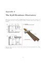
A The Kjell Henriksen Observatory
52
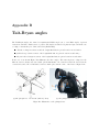
B Tait-Bryan angles
55
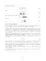
C Calculation of the height of aurora
56
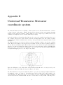
D Universal Transverse Mercator coordinate system
57
E Fragments from the user manual to the SvalPoint system
E.1 What is SvalPoint? . . . . . . . . . . . . . . . . . . . . . . . . . . . .
E.2 How to use SvalPoint? . . . . . . . . . . . . . . . . . . . . . . . . . .
E.3 Format of commands . . . . . . . . . . . . . . . . . . . . . . . . . . .
E.4 Known issues and quick trouble shooting . . . . . . . . . . . . . . . .
E.4.1 SvalCast is not responding after the first command was sent .
E.4.2 SvalCast is not connecting to the servers . . . . . . . . . . . .
E.4.3 Target acquisition failed . . . . . . . . . . . . . . . . . . . . .
E.4.4 Multiple instruments pointing at different targets . . . . . . .
E.4.5 Target acquisition stops unexpectedly . . . . . . . . . . . . .
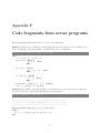
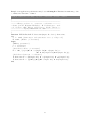
F Code fragments from server programs
.
.
.
.
.
.
.
.
.
.
.
.
.
.
.
.
.
.
.
.
.
.
.
.
.
.
.
.
.
.
.
.
.
.
.
.
.
.
.
.
.
.
.
.
.
.
.
.
.
.
.
.
.
.
.
.
.
.
.
.
.
.
.
.
.
.
.
.
.
.
.
.
.
.
.
.
.
.
.
.
.
.
.
.
.
.
.
.
.
.
.
.
.
.
.
.
.
.
.
.
.
.
.
.
.
.
.
.
.
.
.
.
.
.
.
.
.
59
59
59
61
62
62
62
62
62
62
63
3
List of Figures
1.1
Sketch of the test system used for the implementation of the pointing algorithms. . . . . . .
9
2.1
2.2
2.3
Illustration of the problem solved in the airborne image mapper software. . . . . . . . . . .
All-sky lens model. . . . . . . . . . . . . . . . . . . . . . . . . . . . . . . . . . . . . . . . . .
The graphical user interface of the SvalTrack II software. . . . . . . . . . . . . . . . . . . .
12
14
15
3.1
3.2
3.3
3.4
The
The
The
The
.
.
.
.
16
17
18
18
4.1
4.2
4.3
Overview of the data exchange between the system parts. . . . . . . . . . . . . . . . . . . .
The general network model followed. . . . . . . . . . . . . . . . . . . . . . . . . . . . . . . .
The client-server model of the SvalPoint System. . . . . . . . . . . . . . . . . . . . . . . . .
20
21
24
5.1
5.2
5.3
5.4
Illustration of Cartesian coordinates X, Y, Z and geodetic coordinates ϕ, λ, h. . . . . . . . .
Global and local level coordinates. . . . . . . . . . . . . . . . . . . . . . . . . . . . . . . . .
Measurement quantities in the PSRF. . . . . . . . . . . . . . . . . . . . . . . . . . . . . . .
Top view illustration of the system, showing effect of spatial displacement between the
instrument and sensor . . . . . . . . . . . . . . . . . . . . . . . . . . . . . . . . . . . . . . .
Illustration of the system from the side, showing effect of spatial displacement between the
instrument and sensor. . . . . . . . . . . . . . . . . . . . . . . . . . . . . . . . . . . . . . . .
Calculating the components (x or ni , y or ei , z or ui ) of a vector (v) defined by azimuth (ω)
and elevation (γ). . . . . . . . . . . . . . . . . . . . . . . . . . . . . . . . . . . . . . . . . . .
Calculating the magnitude of vector based on the height of the target. . . . . . . . . . . . .
26
27
29
5.5
5.6
5.7
6.1
6.2
6.3
6.4
6.5
6.6
6.7
6.8
7.1
7.2
Narrow Field of view sCMOS camera.
Fs-Ikea spectrograph. . . . . . . . . .
PTU D46 platform. . . . . . . . . . .
all-sky camera. . . . . . . . . . . . . .
.
.
.
.
.
.
.
.
.
.
.
.
.
.
.
.
.
.
.
.
.
.
.
.
.
.
.
.
.
.
.
.
.
.
.
.
.
.
.
.
.
.
.
.
.
.
.
.
.
.
.
.
.
.
.
.
.
.
.
.
.
.
.
.
.
.
.
.
.
.
.
.
.
.
.
.
.
.
.
.
.
.
.
.
.
.
.
.
.
.
.
.
.
.
.
.
.
.
.
.
.
.
.
.
.
.
.
.
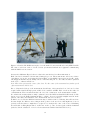
DGPS station and user on Svalbard, at KHO. . . . . . . . . . . . . . . . . . . . . . . . . . .
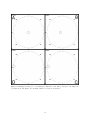
The first target of pointing for the yaw angle calibration. . . . . . . . . . . . . . . . . . . .
Pictures taken of the first target during the yaw calibration. . . . . . . . . . . . . . . . . . .
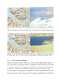
Second calibration target: Adventstoppen. . . . . . . . . . . . . . . . . . . . . . . . . . . . .
The third validation target: Hiorthhamn. . . . . . . . . . . . . . . . . . . . . . . . . . . . .
Examples for images recorded during the calibration of the fish-eye lens. . . . . . . . . . . .
Top view of the calibration set-up. Illustration of the effect of a spatial offset of the rotational
axis of the arm and the centre of the camera. . . . . . . . . . . . . . . . . . . . . . . . . . .
Calculating the angle for the fish-eye lens based on the angle measured in the calibration
system. . . . . . . . . . . . . . . . . . . . . . . . . . . . . . . . . . . . . . . . . . . . . . . .
The distribution of auroral heights. . . . . . . . . . . . . . . . . . . . . . . . . . . . . . . . .
The pointing error as function of height of target and distance between sensor and instrument
if the direction of instrument is the (1,0,0) or (0,1,0) unit vector from sensor and the set
value in SvalPoint for the height of target is 110 km. . . . . . . . . . . . . . . . . . . . . . .
4
30
30
31
32
34
36
36
37
37
39
40
40
44
45
7.3
7.4
7.5
8.1
The pointing error as function of height of target and distance between sensor and instrument
if the direction of instrument is the (0,0,1) unit vector from sensor and the set value in
SvalPoint for the height of target is 110 km. . . . . . . . . . . . . . . . . . . . . . . . . . . .
The pointing error as function of height of target and distance between sensor and instrument
with the height of target 200 km, estimated with 50 km uncertainty. Height set in SvalPoint:
200 km. . . . . . . . . . . . . . . . . . . . . . . . . . . . . . . . . . . . . . . . . . . . . . . .
The pointing error as function of height of target and distance between sensor and instrument
with the height of target 200 km, estimated with 50 km uncertainty. Height set in SvalPoint:
187 km. . . . . . . . . . . . . . . . . . . . . . . . . . . . . . . . . . . . . . . . . . . . . . . .
45
46
46
Validation of the system. . . . . . . . . . . . . . . . . . . . . . . . . . . . . . . . . . . . . . .
49
A.1 Basic design of the observatory. . . . . . . . . . . . . . . . . . . . . . . . . . . . . . . . . . .
A.2 Instrument map of KHO. . . . . . . . . . . . . . . . . . . . . . . . . . . . . . . . . . . . . .
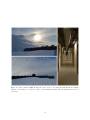
A.3 Photos of KHO. . . . . . . . . . . . . . . . . . . . . . . . . . . . . . . . . . . . . . . . . . . .
52
53
54
B.1 Illustration of the principal axes. . . . . . . . . . . . . . . . . . . . . . . . . . . . . . . . . .
55
D.1 Illustration of the UTM. . . . . . . . . . . . . . . . . . . . . . . . . . . . . . . . . . . . . . .
D.2 UTM grid zones in Scandinavia. . . . . . . . . . . . . . . . . . . . . . . . . . . . . . . . . .
57
58
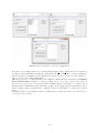
E.1 The user interface of the server applications. . . . . . . . . . . . . . . . . . . . . . . . . . . .
60
5
List of Tables
6.1
6.2
DGPS measurements and their equivalent in geodetic coordinates. . . . . . . . . . . . . . .
Geodetic coordinates of instruments measured with hand-held GPS device. . . . . . . . . .
6
35
35
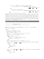
List of abbreviations
API
DDE
DGPS
EISCAT
ETRS89
FOV
GPS
IDE
IP
IWRF
KHO
LTU
PSRF
RAD
SWRF
TCP
UDP
UNIS
UTM
VCL
WGS
Application Programming Interface
Dynamic Data Exchange
Differential GPS
European Incoherent Scatter Scientific Association
European Terrestrial Reference System 1989
Field of View
Global Positioning System
Integrated Development Environment
Internet Protocol
Instrument World Reference Frame
The Kjell Henriksen Observatory
Luleå University of Technology
Pointing System Reference Frame
Rapid Application Development
Sensor World Reference Frame
Transmission Control Protocol
User Datagram Protocol
The University Centre in Svalbard
Universal Transverse Mercator
Visual Component Library
World Geodetic System
7
Chapter 1
Introduction
The Kjell Henriksen Observatory (KHO) is an optical research station focusing on the middle- and upper
atmosphere. It is located in Breinosa, at 15 km distance from the centre of Longyearbyen, on Svalbard,
Norway. During the past two years there has been an acquisition of optical instruments that are capable
of all-sky tracking by the use of 2-axis motorized flat surface mirrors. The observatory has however been
yet lacking an efficient system for the control of these instruments. The goal of this thesis is to define and
develop a real time control system that is convenient to use for observations, ultimately named SvalPoint.
1.1
Project aims
The optical instruments are placed in the instrumental modules of the observatory building. Each module
consists of a dome room, housing the instrument and ensuring a 180◦ visibility to the sky through the roof
of the observatory, and a 1.25 m wide control room, housing a computer dedicated to the instrument. For
the conduction of the observations there is a separate operational room of 30 m2 , large enough to house a
number of work stations, therefore suitable for a group of people to work comfortably at the same time.
(See more information on the KHO building in Appendix A and at KHO (2014c).) One of the problems
desired to be solved is the need of personnel in the control rooms. The new system shall make it satisfactory
to sit only in the operational room, or alternatively to work from Longyearbyen as the travel to KHO, due
to its location, is not possible by car but only by belt wagon or snowmobile during the observational season.
The second problem seeking solution is the acquisition and position determination of targets. An intuitive,
easy solution is desired, with multiple options, easily adapted to future needs. There are a number of
software applications already developed at The University Centre in Svalbard (UNIS) that are suitable for
target location, such as the Sval-X Camera and SvalTrack II (see Sections 2.2 and 2.3 for more information
on the programs). These applications shall be integrated in SvalPoint as user interfaces for finding and
locating the target.
An additional goal for the system is to enable simultaneous control of multiple instruments, possibly
installed at different locations, pointing them at the same target; hence acquiring the name multi-track
optical pointing system. This will enable a large range of observations not possible before at the observatory.
8
1.2
Task analysis
To meet the goals defined in Section 1.1 the main problems to be solved in the projects are:
design of the system as a software package: what are the functionalities of different applications
working together, description of the new programs that need to be developed,
definition of control methods for the instruments: how is the target defined, what is the information
needed about it,
design of the connections between the programs: used communication protocols and the definition of
high-layer protocols,
development of algorithms controlling the instruments for each of the defined pointing methods,
definition of calibration parameters and methods.
Regarding the instrument control problem, the pointing is done by the operation of two motors. The control of their motion is done by azimuth and elevation angles from the spherical coordinate system. Motor
controller units are connected to each pair of motors, therefore their control is possible by command words
sent on serial ports, making the extent of this work to be that of high level, logical control.
The tasks at hand are:
finding optimal solutions to the problems listed above,
the implementation of the new programs,
calibration of the system,
performance evaluation,
validation of SvalPoint.
During the practical work related to this thesis the software development and the solving of the problems
are done in parallel by exploring possibilities, trying out methods, identifying necessities.
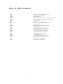
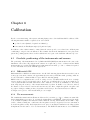
An additional problem to be solved is that of work arrangements due to the remote location of the observatory. A test system using a pan-tilt unit mounted on a tripod, pointing a web-camera has been installed
at UNIS, therefore the need for visiting KHO during the implementation and testing of the algorithms is
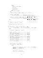
eliminated. See the sketch of the system in Figure 1.1.
Figure 1.1: Sketch of the test system used for the implementation of the pointing algorithms.
9
1.3
Outline of Thesis
This thesis presents the software applications that form the SvalPoint system and their interaction. The
protocols and algorithms used for the pointing control of the instruments is presented in detail, being the
major contribution of this project apart from the definition and creation of the system. Furthermore the
calibration processes related to the system are also described in addition to the validation and conclusions
about the system.
Chapter 2 presents projects that precede SvalPoint, conducted at UNIS. The first section describes a software solving similar coordinate-system change problems as the ones met in this project. Lastly, the second
and third sections describe the programs used in the SvalPoint as user interfaces for target acquisition.
In Chapter 3 the reader will find a description of the hardware used in SvalPoint. Some terminology used
further on is defined and the different instruments operated by SvalPoint are shortly summarized.
In the first part of Chapter 4 the components of the system are described, along with their interaction, communication protocols, including high layer protocols defined during the project. The last section presents
what operational errors are detected in SvalPoint and the actions taken at their appearance.
Chapter 5 starts with the definition of naming conventions used for the description of the algorithms. In
the followings the algorithms on the server side are presented, used for the pointing of the instruments.
Chapter 6 describes the necessary calibration processes for the system along with details regarding the
calibration done during the practical work.
Chapter 7 is dedicated to the discussion of accuracy. All factors contributing to it are described with
numerical calculations where possible.
In Chapter 8 the tests necessary for the validation of the system are defined. Further on the partial validation of the system is presented together with expected results for the final trial (as in contrast to the
present results).
Finally Chapter 9 summarizes the conclusions of the thesis and presents some suggestions for future work
to enhance the existing system.
10
Chapter 2
Previous projects at UNIS
This chapter presents projects related to the SvalPoint system that has been studied during the work process
or used directly in the system. The SvalPoint system is preceded by two standalone software applications,
the Sval-X Camera and SvalTrack II that are used as parts of SvalPoint with minimal modifications.
The airborne image mapper software on the other hand is presented and studied as a similar application
in some aspects and solutions in it are adapted in the new programs of the SvalPoint.
2.1
Airborne image mapper
The airborne image mapper is a software that projects photos taken by a camera mounted on a helicopter
to the Google Earth map as part of a large project at KHO, presented in Sigernes et al. (2000). By knowing
the location of the helicopter in geodetic coordinates, its attitude and the initial orientation of the camera
in reference to the vehicle carrying it, the location of the picture is identified. In other words this program
solves the transformation of points defined in a local reference frame, in the image, into points in world
reference frame, identifying their place on the map.
The same transformation is a key element of any pointing system for multiple instruments based on target identification by a sensor. The target at first is found and defined in comparison to the sensor, in
its local reference frame. To find the independent position, a similar algorithm shall be used as in the
airborne image mapper that transforms the location into world reference frame. Later, when the scientific
instruments shall be pointed at the target, the location is transformed from the world reference frame into
the local reference frame of each instrument apart, doing the same transformations in the opposite direction.
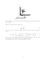
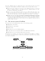
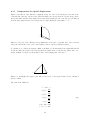
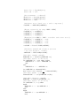
The algorithm used in the Airborne image mapper software is called Direct Georeferencing, the problem
being illustrated in Figure 2.1. Point P’ is the point identified in the image taken by the camera, this being
the four corners of the picture in the program. P is the point sought, that in reality, of which the image is
taken through the focal point.
The local level coordinate system, placed in the focal point of the camera is noted by X1 Y1 Z1 , while the
world reference frame is X2 Y2 Z2 (see Figure 2.1). The position of the point in reality, v p , represented in
world reference frame (X2 Y2 Z2 ) is:
v p = v o + λ · DCM · v i ,
(2.1)
where v o is the position of the local coordinate system’s origin in the world coordinate system, λ is a scale
factor specific for the lens used relating P to P’, DCM is the direct cosine matrix for the rotations that
transform a vector in the local reference frame into the world reference frame and v i is the position of point
P’ in the X1 Y1 Z1 coordinate system.
11
Z2
X1
P’
Y1
vo
Z1
vp
Y2
P
X2
Figure 2.1: Illustration of the problem solved in the airborne image mapper software. Image adapted from
Sigernes (2000).
Furthermore expressing the terms of Equation (2.1):
xi
v i = yi ,
f
(2.2)
where xi and yi are the two Cartesian coordinates of point P’ in the image, f is the focal length of the
lens; and
1
DCM = 0
0
cos(ψ) sin(ψ)
cos(θ) 0 −sin(θ)
0
0
1
0 −sin(ψ) cos(ψ)
cos(σ) sin(σ) 0
0
0
sin(θ) 0 cos(θ)
−sin(σ) cos(σ)
0
0 ,
1
(2.3)
where σ, θ and ψ are the roll, pitch and the yaw angles respectively for the attitude of the local coordinate
system in relation to the world reference frame. See also Muller et al. (2002).
The equations presented are adapted to the SvalPoint system, see Chapter 5.
12
2.2
Sval-X Camera
The Sval-X Camera is a software developed at UNIS, that collects image feed from any camera connected
to the computer, given that its driver is installed and it has DirectShow application programming interface
(API). The software contains numerous functions for video and image processing, such as: tracking of an
object in the video or summing up a user-defined number of frames to get a sharper and more clear image
of a static object. The program is used as a possible user interface for control in the SvalPoint system with
minimum modification.
One of the functions in the control interface of Sval-X Camera is the video overlay for all-sky cameras.
This overlay indicates the cardinal directions in the image, in addition to showing the line of horizon. The
necessary attitude and position information for this overlay may come from both a gyroscope - GPS pair,
as dynamic values, or can be static calibration inputs. It also calculates the direction to a target, identified
by a click on the image, defining the azimuth and elevation angles for that point from the origin of the
’lens coordinate system’ (placed in the optical centre of the lens, aligned with the direction of the axis
of focus). The values are later transformed into a local level world reference frame, placed in the centre
of the lens, aligned with north-east and up directions, making the direction of target independent of the
orientation of the camera, the only dependency remaining: its geodetic location. These calculations give
information about the location of target used for the control of instruments. In the followings the method
for calculating the angles in the lens coordinate system is presented.
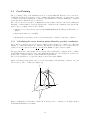
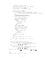
Considering a fish-eye lens, that all-sky cameras use, Figure 2.2 can be drawn with two coordinate systems
associated with the camera: the coordinate system of the lens, noted by X1 Y1 Z1 and the coordinate system
of the image plane: X2 Y2 Z2 . The focal length of the lens is f. The aim is to define the direction to P (point
in the real world) based on the position of P’ (point in the obtained image), indicated in Figure 2.2. The
position of P’ can be determined in the image by the values r (the distance between P’ and the centre of
the image coordinate system) and ψ2 (angle between axis Y2 and r). The direction of point P in X1 Y1 Z1
shall be defined by the direction of vector ρ, in spherical coordinates.
According to Kannala & Brandt (2004) the fish-eye lenses are usually designed to obey one of the following
relations for projections:
r = 2 · f · tan(θ/2) (stereographic projection),
r = f · θ (equidistance projection),
r = 2 · f · sin(θ/2) (equisolid angle projection),
(2.4)
r = f · sin(θ) (orthogonal projection).
All four expressions are implemented in the Sval-X Camera application, subject to user settings. In the
following the relations are to be developed with the use of the most common type of fish-eye lens, with
equidistant projection.
Based on Equation (2.4) and Figure 2.2:
r = r(θ) = f · θ,
x2 = r(θ) · sin(ω2 ),
y2 = r(θ) · cos(ω2 ),
(2.5)
z2 = f.
It shall be noted that due to the fact that the lens is circular:
ω1 = ω2
(2.6)
From Equations (2.5) and (2.6) the value of θ and ω1 can be calculated directly. These values represent
the azimuth and elevation of the point in X1 Y1 Z1 , based on the image captured by the all-sky camera.
13
Z1
P
ρ
Y1
θ
ω1
X1
Z2
f
X2
r
ω2
image plane
P0
Y2
Figure 2.2: All-sky lens model. Figure adapted from Kannala & Brandt (2004).
The robustness of the software is guaranteed by input for the attitude of the instrument. This is used on
one hand to be able to place the projection of the point in a local level, world reference frame, not related
to the orientation of the camera, and on the other hand to calculate and draw the line of horizon on the
picture captured by the instrument.
The application of the rotational matrix and hence the disconnection of the coordinates from the camera’s
orientation is done with the use of rotation matrices, see the previous section and related parts in Chapter 5.
In order to be able to apply them, the vector shall be expressed with Cartesian components, the equations
for the transformation are given in Chapter 5.
14
2.3
SvalTrack II
The SvalTrack II software (see Sigernes et al. (2011)), developed at UNIS, is a sky observer program. It
implements different models for the determination of the auroral oval, information about celestial bodies
and satellites. It is a real time software, updating the information about all the previously mentioned in
each second, providing azimuth and elevation information about them from the geographic position of the
program (subject to user setting). Satellite information is extended with their altitude as well.
This program is used as another possible instrument control interface of the SvalPoint. As it does not use
any sensor for target acquisition, it is considered to be a mathematical control interface and henceforth it
is referred to as such.
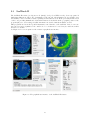
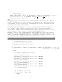
See Figure 2.3 for screen captures of the software’s graphical user interface.
Figure 2.3: The graphical user interface of the SvalTrack II software.
15
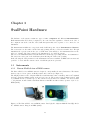
Chapter 3
SvalPoint Hardware
The hardware of the system contains two types of units: computers and different instrumentation.
Each instrument has its dedicated computer for its control and the acquisition of data from it. One of
the computers acts as the controller of the SvalPoint system that can be separate or one connected to an
instrument.
The instrumentation falls in two categories from the SvalPoint’s point of view: Instruments and Sensors.
The instruments are the units controlled through pointing and they collect the scientific data. Though
instruments is a generic term, in the case of SvalPoint it refers strictly to the instruments that are the
subject to pointing. The data acquired by the instruments do not affect the system.
The sensors are instruments that collect information about the target, providing a mean to its identification.
The sensors are active part of the SvalPoint system affecting the result of the pointing.
In the following the basic parameters of the instruments and sensors available at KHO at the moment and
possible to be used with the current version of SvalPoint system are presented.
3.1
3.1.1
Instruments
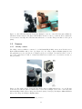
Narrow Field of view sCMOS camera
The Narrow Field of view sCMOS camera is designed to study small scale auroral structures. The instrument is composed of two parts: an all-sky scanner and a camera (see Figure 3.1).
The All-Sky scanner is a Keo SkyScan Mark II, a dual first-surface mirror assembly, with a 360◦ azimuth
and a 90◦ elevation scanning, put into motion by servo motors. The accuracy of the pointing is ±0.05◦ with
9◦ /s azimuth and 27◦ /s elevation speed. The camera used is an Andor Neo sCMOS, on a -40◦ C vacuum
cooled platform, mounted with a Carl Zeiss Planar 85 mm ZF lens with a relative aperture of f/1.4. See
KHO (2014b).
Figure 3.1: The Narrow Field of view sCMOS camera. Panel (A): Keo SkyScan Mark II. Panel (B): Andor
Neo sCMOS camera. Image from KHO (2014b).
16
3.1.2
Hyperspectral tracker (Fs-Ikea)
The Hyperspectral tracker is a narrow field of view hyperspectral pushbroom imager. The instrument
composes of two parts: an all-sky scanner and a spectrograph (see Figure 3.2).
Figure 3.2: Panel (A): The Fs-Ikea spectrograph with its protective covers off. (1) Front lens, (2) Slit
housing, (3) Collimator, (4) Flat surface mirror, (5) Reflective grating, and (6) Camera lens. Panel (B):
All-Sky scanner. Image from KHO (2014a).
The spectral range of the instrument is between 420 and 700 nm, with a bandpass of approximately 1 nm.
The exposure time for one spectrogram is approximately 1 s. One of the possible lenses to be used is a
Carl Zeiss Planar 85mm ZF with the relative aperture f/1.4.
The all-sky scanner is composed of two first surface mirrors, mounted on two stepper motors. The azimuth
range of the instrument is 360◦ , while the zenith angle range is ±90◦ . The resolution of the motion is
0.0003◦ with an accuracy of ±0.05◦ . See more at KHO (2014a).
3.1.3
Instrument constructed on the PTU D46 platform
The PTU D46 is a pan-tilt unit suitable to point any instrument weighing up to 1.08 kg, in a range ±159◦
in azimuth and 31◦ down and 47◦ up in elevation with resolution of 0.0129◦ (Directed Perception 2007).
This unit is used widely at KHO, mainly pointing cameras with different lenses. One example for its use is
the Tracker Camera, a mount of the Watec LCL-217HS colour and the Watec 902B monochrome camera
on a PTU D46 unit. The lenses used are 30 mm Computar TV Lens with a relative aperture f/1.3 (for the
colour camera) and a 75 mm Computar lens with f/1.4 (for the monochrome camera). This instrument
is used to provide a live feed on the internet at the KHO web page (KHO 2014e). See Figure 3.3 for an
image of the Tracker Camera and the PTU D46 unit.
17
Figure 3.3: The PTU D46 platform. Panel (A): Example for the use of the PTU D46 unit at KHO: the
instrument Tracker Camera. The Watec LCL-217HS is mounted on the top, while the Watec 902B is the
bottom camera. Panel (B): The PTU D46 unit with its motor controller. Image from Directed Perception
(2007).
3.2
3.2.1
Sensors
All-sky camera
The all-sky camera at KHO is constructed of a DCC1240C-HQ C-MOS camera from Thorlabs and a
Fujinon FE185C046HA-1 fish-eye lens. (See Figure 3.4.) According to Fujinon Fujifilm (2009) the lens
has equidistant projection (f θ system, see Equation (2.4)), a focal length of 1.4 mm and a field of view of
185◦1 . The camera has a resolution of 1280 x 1024 Pixels and a sensitive area of 6.78 mm x 5.43 mm, see
Thorlabs (2011).
Figure 3.4: The all-sky camera. Panel (A): The all-sky camera at KHO with its lens cover off. The ring
around the lens with the spike is a sun-blocker to avoid direct sunlight on the sensor. Panel (B): The
DCC1240C-HQ C-MOS camera. Image from Thorlabs (2011). Panel (C): The Fujinon FE185C046HA-1
fish-eye lens. Image from Fujinon Fujifilm (2009).
1 The
field of view has been found to be 194◦ during calibration.
18
Chapter 4
Software design
The design of the system as a collection of software applications, the scope of each program and their
interaction is one of the main contributions of this thesis. The final structure has been defined well in the
development of the software by identifying needs, and trying out different alternatives. The end result of
this process is presented in this chapter.
4.1
System definition
The aim of SvalPoint is to fill in the existing gaps in the current process of instrument operation. The
system shall provide easy options for target location and acquisition and link it to the pointing of the
instrument, eliminating the necessity for presence in the control room (see Section 1.1 for the complete
description of project aims). The acquisition of data from the target instruments is already automated,
solved for each instrument apart, independent of the SvalPoint system.
The SvalPoint system is composed of three parts:
a control interface, which can be any of the two already existing applications developed at KHO:
SvalTrack II or Sval-X Camera, with the responsibility of acquiring the target and determining its
location;
server programs, dedicated to each instrument and installed on the computers in the control room
with the responsibility of pointing the instrument, developed in the duration of this thesis project;
a client program that acts as a data transmitter between the control interface, and the server
applications, its responsibility being to transfer the commands and all necessary information to the
server and to display the messages sent as feedback from the server; this program is also developed
during the work associated to this thesis.
At the definition of the system there has been two options to consider: either to integrate the client application into the control interface programs, or to develop a separate software for it. The decision fell on
the latter one for the following reason: the user interface programs implement many functionalities already
and there was no room planned for such an extension from the beginning of their development.
The control interface programs are preferred to provide a continuous data stream without waiting for response, sending positions at regular time intervals. The reason for this is that in case there is hold-up for
feedback the control interfaces would not be able to update their real time features such as the basic video
acquisition or the tracking of an object.
Displaying feedback from the instruments in the client is considered not a vital, however a highly desired
feature. Since the locations of the control personnel and the instrument can be kilometres apart it is
helpful to know whether the command has been executed or not. One might argue that it is visible from
the images captured by the instruments. However there might be exceptions to this assumption, such as
in case the images are not streamed over the internet, but saved on the local drive. Moreover the isolation
19
of problems in control and data acquisition would not be possible.
As what regards the continuous command stream, that is not desired on the server side since reading,
interpreting, executing and confirming the execution of commands takes time, this being true even in case
the command was the same as the one before. This lead to the very logical design decision: the same
commands shall be filtered out from the stream, leaving only the ones that change the pointing of the
instrument. As the servers are aimed to be kept general, simple and easy to use, it is the client program
that is desired to act as the filter of the data stream.
The functionalities of the servers are therefore defined to include the reading of the commands, the interpretation and calculation of the direction of pointing, and the sending of feedback to the client upon
execution. See Appendix F for code fragments from the server programs. The client application, named
SvalCast, is defined to be responsible for the reading of the data from the control interface programs, the
filtering of the stream and the sending of the commands to the servers. The control interface from the
system’s point of view is responsible for providing a stream of pointing directions for the instruments. See
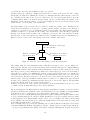
Figure 4.1 for an overview of the data exchange between the elements of the system.
Control interface
Information stream about the target
from control interface
Client
Filtered command
stream from client
Server 1
Feedback about execution
of commands from server
Server 2
...
Server n
Figure 4.1: Overview of the data exchange between the system parts.
The pointing methods for the instruments defined, that all servers must be able to execute, fall into two
main categories. The first category is the target-independent commands, with only one command falling in
it, the HOME command. This command sends the instrument to its home position defined by the control
unit. The second category is pointing at target which can be defined either by geodetic location, the method
being called geo-pointing, or by azimuth and elevation of target acquired from a sensor, accompanied by
information about the sensor location and height of target (indicating the length of the vector between the
sensor and target). The latter, referenced to as direction based pointing henceforth, may have two options:
when the range of the target is unknown and the target is considered to be infinitely far away; and when
the range can be estimated by estimating its height of target above the reference ellipsoid. The algorithms
used for the different methods are described in the Chapter 5.
It shall be noted that none of the current control interfaces point the instruments by the use of geodetic
coordinates. At the moment this feature is used only in calibration.
The chosen language for the implementation of the applications is Delphi for a number of reasons. Foremost
all other programs associated with the control of the instruments, developed at KHO are in Delphi making
it the first choice due to considerations of program extension, maintenance or future changes.
Another reason for choosing Delphi is that the applications require a graphical user interface that is tedious
to develop in many languages, in contrast to Delphi. Delphi has been developed with the aim of providing
a rapid application development (RAD) software, based on a set of intuitive and visual tools that help
the programmer. The user interfaces are constructed visually, using a mouse rather than by coding, that
greatly helps in visual interface development.
Moreover Delphi offers object oriented programming, based on Pascal, with its own integrated development
environment (IDE). The IDE also implements a debugger, offering options for setting breakpoints in the
code, step by step running and the display of the values of variables, all helping the program development
20
process greatly.
4.2
Communication between programs
The applications defined in Section 4.1 shall be connected among each other to be able to transfer the
required data. Two types of connections are needed: a connection between the server and client and one
between client and control interfaces.
As discussed in Chapter 1 as well, it is desired to have a remote control over the server programs from any
location. This goal demands a connection with Internet Protocol (IP) between the client and the server,
one that is suited to transfer short strings. The best way to establish a communication optimal for this
task has been identified to be a network socket. Two transport protocols has been considered: the User
Datagram Protocol (UDP) and Transmission Control Protocol (TCP). The TCP has been chosen as it is
well suited for applications that require high reliability, however transmission time is not critical. In TCP
there is absolute guarantee that the data transferred remains intact and arrives in the same order in which
it was sent by the establishment of an enduring connection between computer and remote host. In contrast
the UDP is faster but it does not guarantee that the data arrives at all, a major disadvantage over the
TCP in this case. See Section 4.2.1 for more information on the TCP protocol.
The control interface and client run on the same computer, therefore any connection that ensures communication between two programs in Microsoft Windows is satisfactory as long as the communication is
fast enough for handling the data stream. Two options are considered, one of them being the use of the
clipboard, the other one the Dynamic Data Exchange. The clipboard is however already in use by the control interface applications for communication with different small programs, and as the protocol provides
no mean of targeting the data written to it, this option is discarded, leaving the Dynamic Data Exchange
as the mean of communication. See Section 4.2.2 for more information on the Dynamic Data Exchange
protocol.
The client-server model followed is presented in Figure 4.2. There are several control interfaces that can
command the client to which multiple servers are connected through the internet. It shall be noted, that
despite the possibility to start multiple control interfaces at the same time, it is counter-advised. It is not
restricted due to possible advantages of this feature, however unintentional use shall be avoided by always
closing one control interface before opening another.
Control Interface 1
DDE
Control Interface 2
DDE
...
Control Interface n
DDE
Client
TCP socket
Internet
TCP socket
Server for Instrument 1
TCP socket
Server for Instrument 2
TCP socket
...
Server for Instrument n
Figure 4.2: The general network model followed.
One of the challenges in the development of the system is to make the programs ’freeze’-proof. At the usage
of any system one of the most irritating things is when one of the programs stops responding to commands
and must be closed from the Command Manager of Windows. That happens each time an exception is
thrown and it is not verified and treated in the code. The connections between programs throw a large
number of exceptions (e.g. the client is not responding, the connection cannot be established) therefore a
special emphasis is placed on their treatment during the development of the software applications.
21
The security of the system is mainly ensured by the firewall on the computers, blocking any attempts for
connection coming from another computer than one registered in the KHO network. The security related
considerations implemented in the servers are the verification of command formats and values.
4.2.1
TCP socket
The TCP socket is the endpoint of inter-process communication flow based on internet protocol between
server (sender of data) and client (receiver of the information). The client application establishes point to
point virtual connection, also known as TCP session, between two sockets defined by IP address (identifying
the host interface) and port number (identifying the application and therefore the socket itself). The server
applications create sockets that are ’listening’ and responding to session requests arriving from clients.
An internet component suit in Delphi 5 is provided by Indy (Internet Direct) in the form of a Visual
Component Library (VCL). The Indy.Sockets includes client and server TCP sockets and it has been used
in the implementation of all servers and the client application.
Indy makes the program development very fast, however it does have one downside: it uses blocking socket
calls. Blocking socket calls mean that when a reading or writing function is called it does not return until
the operation is complete. Due to this it is very easy to program with these functions, however they block
the thread of the application, causing the program to ’freeze’: it does not respond to any command and it
need to be closed from the Task Manager. This would be a major problem if a continuous data stream was
sent over the TCP sockets. However, as explained earlier in this chapter this problem has been out-ruled
by design. Another implication of the blocking sockets is that during implementation special attention
shall be paid so that each message sent over the socket is read on the other side of the communication.
(Hower, C. Z. & Indy Pit Crew 2006)
4.2.2
Dynamic Data Exchange
The Dynamic Data Exchange (DDE) is a protocol in Microsoft Windows for fast data transfer between
applications that was introduced to exchange the clipboard operations in 1987. Each side of the communication, both the server and the client of the DDE data transfer may start a conversation by transferring
data or requesting data from the other. The role of the server and client can be switched during one session
and there may be multiple clients in the conversation. (Swan 1998)
In the case of the control interface and client (SvalCast) connection the communication is one-way. SvalCast acts as the client in the DDE, while the control interface is the server. Once the communication is
established there is a continuous data stream between the two applications.
4.2.3
SvalPoint high-layer protocols
The SvalPoint system has two different high-layer communication protocols defined: information format
for data communication between control interface and client, and command formats for server control.
Control interface - client protocol
The control interface and client protocol communication must contain the following information: the geodetic location of the observation (latitude and longitude in degrees, altitude in metres), the direction of target
(azimuth and elevation in degrees) and the altitude of the target in kilometres. A target altitude equal to
zero indicates the lack of information on the altitude, in which case the target is considered infinitely far
away.
Note: As the geo-pointing is not possible at the moment through the control interfaces no protocol has
been defined for it yet.
The control interface sends one string of characters to the client containing information in the following
format:
’A ’+[latitude]+’ B ’+[longitude]’+’ C ’+[altitude]+’ D ’+[azimuth]+’ E ’+[elevation]+’ Z ’+[altitude of
target]+’ S’.
22
Client - server protocol
The client-server communication is bidirectional. The client sends commands to the server to control the
instruments, while the server sends a feedback to the client about the success of the execution of commands.
The protocol for messages sent by the client to the server is based on command words to indicate different
ways of control. The protocol is based on strings following each other in separate messages. There are five
command words. Some are stand-alone, basic commands, while others must be followed by different values
in a given order.
The commands are as follows:
HOME (alternatively: home or Home) - The keyword HOME sends the instrument to its home
position, defined as home positions for the motors. This command is not followed by any value.
Note that this position is not equivalent to sending 0 azimuth and elevation values to the instrument.
GPS (alternatively: gps or Gps) - The keyword GPS must be followed by 3 numbers in the following
order: geodetic latitude in degrees, geodetic longitude in degrees and altitude above reference ellipsoid
in metres. Through this command the target of pointing is defined through its geodetic coordinates.
Note that the convention is negative values for East and South.
Example: GPS 78.15 -16.02 445
AZEL (alternatively: azel, Azel or AzEl) - The keyword AZEL must be followed by five values
representing the geodetic location of the sensor (latitude in degrees, longitude in degrees and altitude
above reference ellipsoid in metres), and the azimuth and elevation angle for the direction vector to
the target in degrees in the order described.
Example: AZEL 78.147686 -16.039011 523.161 12.6 25.1
AZELH (alternatively: azelh, Azelh or AzElH) - The keyword AZELH must be followed by six
values. It is the same five values as for the AZEL adding the height of the target above ground in
km as the sixth parameter.
Example: AZELH 78.147686 -16.039011 523.161 12.6 25.1 200
END (alternatively: end or End) - Ends the connection between the client and server application.
There are no values following this command.
Any feedback from the servers is a single string that forms a message sentence directly displayed in the
client application, without any interpretation.
4.2.4
Erroneous commands and feedback to client
To avoid cases in which the client sends commands too fast, the server application always waits for the
execution of the motion by the instruments. An inquiry to the motion control unit is sent regarding the
current position and the program is blocked in a ’while’-loop until the expected response (indicating that
the instrument is in the desired position) is sent on the COM port. As soon as the response is satisfactory
a feedback string is sent to the client, containing the ’Command executed.’ sentence.
This mechanism relies on the assumption that all commands sent to the instruments are correct and possible to be executed. According to this method once the command is sent on the COM port the program
is blocked until the motion is executed and the correct feedback is received. This is a hazard for program
’freeze’, in consequence another condition is added to end the ’while’-loop: the expiration of a timer started
when the control command was sent to the instrument. It is however not desirable for the while loop to
end with the timer expiration (as it takes longer time than the execution of the maximum range of motion
by the instrument), therefore it is made sure that all erroneous commands are filtered out.
Erroneous commands might appear in three situations: the command word is not recognized, the values
following the command word are not correct or the instrument cannot execute the motion due to limitations
in its motion range.
23
In case the command word is not recognized by the server, no action is taken. For other erroneous cases
an appropriate feedback with the words ’Error in command.’ is sent to the client. These cases are:
Number expected and something else received. Some of the command words expect to be followed by
numbers, for example the GPS word. An example for incorrect command is ’GPS 7k.5 -15,4 500’.
Note that the decimal separator is the full stop.
Values not in range. For each number the values are expected to fall in a defined range. The geodetic
latitude value must fall in the [-90, 90) range, the longitude into [-180, 180), the altitude of the
position and of the target must be positive, the azimuth and elevation must be between [0,360).
Resulting angles out of range. The control units have a maximum and minimum value for the angles
that can be set in the server applications. These values are different for the different instrument
control units. For example the PTU D46 unit cannot set greater elevation angles than 47◦ . Therefore
a command that results in such an elevation value in its server application returns the ’Error in
command.’ string to the client.
4.3
The current version of SvalPoint
The current version of the SvalPoint system is composed of the following programs:
SvalTrack II as control interface;
Sval-X Camera as control interface;
SvalCast as client;
Fs Ikea Tracker as server for the Fs-Ikea instrument;
Keo Sky Scanner as server for the Narrow Field of view sCMOS Camera instrument;
PTU46 Tracker as server for the Tracker Camera and the test system.
The client-server model adapted to the current version of SvalPoint is shown in Figure 4.3. It shall be
noted that any of the applications may be modified as long as the interface requirements are kept, ensuring
the robustness of the system.
SvalTrack II
Sval-X Camera
DDE
DDE
SvalCast
TCP socket
Internet
TCP s.
Fs Ikea Tracker
TCP s.
Keo Sky Scanner
TCP s.
PTU46 Tracker
Figure 4.3: The client-server model of the SvalPoint System.
24
Chapter 5
Pointing algorithms
The pointing algorithms are all implemented on the servers side and they are responsible for the calculation
of pointing direction for each instrument based on the information received from the client.
Before discussing the implementation of the different pointing modes, a set of reference frames is to be
defined for the system:
The Sensor World Reference Frame (SWRF) is defined as a Local Level Coordinate System
associated with the sensor. This is the coordinate system in which the commands from the client
application are received in case of direction based pointing command. It is a left handed coordinate
system: X axis is aligned with True North (referenced to as N), Y axis with East (referenced to as E)
and the Z axis with Up (referenced to as U). Its origin coincides with the centre of the sensor lens,
or in case of a mathematical control interface, the origin is the point specified as point of observation
in the application.
Another Local Level Coordinate System, referred to as the Instrument World Reference Frame
(IWRF) is defined. This reference system is identical with the SWRF in all aspects but one: its
origin coincides with the centre of the instrument’s lens. A vector in this reference frame shows the
direction in World Coordinates where the instrument shall point to acquire an image of the target.
The Pointing System Reference Frame (PSRF) is the reference frame in which the instrument
is controlled. The origin of this coordinate system is in the intersection of the two axis along which
the instrument is controlled by the motors, translated by a vector T, and rotated by the Tait-Bryan
angles (see Appendix B ), compared to the IWRF. The XOZ plane in this reference frame is the plane
in which the elevation control motor motion takes place. The YOX Plane is defined by the motion
plane of the azimuth control motor. The X axis of the frame is defined by the intersection of the two
planes, pointing in the direction of the instrument’s optical axis when the control motors are in their
home position. The Z axis points upwards, in the plane of the elevation control motor, perpendicular
to X. Y axis complements the coordinate system to a left handed reference frame. The control of the
instrument is done in the PSRF, therefore all pointing algorithms calculate the target’s direction in
this coordinate system.
In Chapter 4 the principles of the two different target-based pointing modes have been presented. The
geo-pointing mode takes as input the geodetic latitude, longitude and altitude of the target. Knowing
the geodetic coordinates of the instrument the vector between the two points is to be calculated. The
vector is calculated in IWRF, then transferred to the PSRF.
In the direction based pointing mode the target is defined by its direction in the Sensor World Reference
Frame. The server application, in addition to the direction, receives the geodetic information about the
location of the sensor, making it possible to calculate the direction of pointing for the instrument in
Instrument World Reference Frame. The result then is transformed it into the Pointing System Reference
Frame.
25
5.1
Geo-Pointing
The geo-pointing control of the instrument is based on an algorithm that finds the vector between two
points defined by their global level (geodetic) coordinates. The input for this type of control is the geodetic
coordinates of the target, requiring the coordinates of the instrument to be known. Finding the coordinates
for the system is a calibration step, see Chapter 6.
The control of the motors is based on azimuth and elevation angles. Therefore all vectors calculated in
Cartesian coordinates shall be represented in spherical coordinates for the commands of the system. The
steps for the geo-pointing control are the following:
1. Calculate vector between the two given points in IWRF (Instrument and Target), in Cartesian coordinates.
2. Represent the same vector in PSRF.
3. Transform the representation of the vector from Cartesian coordinates to spherical coordinates.
5.1.1
Calculating the vector between points defined by geodetic coordinates
Two points are considered, noted by Pi and Pj , defined by their global level coordinates (ϕi - ellipsoidal
latitude, λi - ellipsoidal longitude, hi - altitude). The aim is to calculate the vector between these two
points, noted by xij , expressed by the ni , ei and ui in the IWRF: a local level reference frame.
The approach used is to first calculate the vector in global level Cartesian coordinates, in the coordinate
system XYZ, with its origin in the centre of the Earth. Finding this vector is a subtraction operation once
we know the coordinates of the two points in Cartesian representation.
The vector found then is to be represented in the local reference frame, IWRF.
Therefore the first problem that needs to be solved is the finding of the Cartesian coordinates of a point
based on the geodetic coordinates (see Figure 5.1).
Z
P
b
N
λ
ϕ
Y
a
X
Figure 5.1: Illustration of Cartesian coordinates X, Y, Z and geodetic coordinates ϕ, λ, h. Figure adapted
from Hofmann-Wellenhof et al. (2001).
26
According to Hofmann-Wellenhof et al. (2001) the relations for these calculations are:
X = (N + h) · cos(ϕ) · cos(λ),
Y = (N + h) · cos(ϕ) · sin(λ),
2
b
N + h · sin(ϕ),
Z=
a2
(5.1)
where N is the radius of curvature in prime vertical, obtained by the relation:
N=p
a2
a2 cos2 (ϕ) + b2 sin2 (ϕ)
,
(5.2)
and a, b are the semi-axes of the ellipsoid.
The parameters of the ellipsoid that models Earth are defined in numerous different standards, such as
the World Geodetic System, WGS 84, the European Terrestrial Reference System, ETRS 89 or the North
American Datum, NAD 27 and NAD 83, just to mention but a few. These standards use different reference
ellipsoids. The coordinates for the target might be acquired with two methods: using maps or using GPS
system. The mapping in Europe is done based on the ETRS 89, while GPS systems use WGS 84. The
two standards use different reference ellipsoids: the ETRS 89 uses GRS1980, while the WGS 84 has its
own reference ellipsoid named WGS 84. Since the coordinates of the target points are most likely to be
obtained by the use of a map, ETRS 89 is used for the definition of the ellipsoid.
According to Geographic information - Spatial referencing by coordinates (2003) the parameters for a and
b defined by the GRS1980 reference ellipsoid are:
a = 6378137.0 m - semimajor axis of ellipsoid,
b = 6356752.3 m - semiminor axis of ellipsoid.
(5.3)
Xi and Xj are defined as the vectors from the centre of Earth to Pi and Pj expressed with Cartesian
coordinates. Then the vector between the two points expressed in Cartesian coordinates is X ij = X i − X j .
Z
ui
ni
Pi
b
ei
Xi
λi
ϕi
Y
a
X
Figure 5.2: Global and local level coordinates. Figure adapted from Hofmann-Wellenhof et al. (2001).
27
To transfer the vector into the local level reference frame first the axes of the IWRF shall be found in global
level Cartesian coordinates (XYZ). The point of origin for IWRF in global level geodetic coordinates is
known (the position of instrument). The vectors ni , ei and ui need to be found that define the directions
true North (ni ), East (ei ) and Up (ui ). (See Figure 5.2)
Illustrated in Figure 5.2 and according to Hofmann-Wellenhof et al. (2001) these vectors are defined by:
−sin(ϕi ) · cos(λi )
−sin(λi )
cos(ϕi ) · cos(λi )
ni = −sin(ϕi ) · sin(λi ) , ei = cos(λi ) , ui = cos(ϕi ) · sin(λi ) .
(5.4)
cos(ϕi )
0
sin(ϕi )
Finally, according to Hofmann-Wellenhof et al. (2001), the expression for the vector xij in IWRF can be
found by the scalar multiplication of its Cartesian coordinates with the vectors expressing the axes of the
local level reference frame. Therefore the last piece of the series of expressions we have been looking for is:
ni · X ij
nij
(5.5)
xij = eij = ei · X ij .
nij
ui · X ij
5.1.2
Transferring vector from IWRF into PSRF
To find a vector in the PSRF (xPSRF ) based on its representation in the IWRF (xIWRF ) a translation and
a rotation shall be performed.
The spatial offset between the centre of the IWRF and PSRF is T, as discussed in the beginning of Chapter
5 (represented in IWRF). The translation is done by subtraction of the vector components of T.
After the translation, the rotation of the coordinate system around the vector shall be performed, with
use of rotation matrices for the transformation. The rotation angles are defined as roll, pitch and yaw
rotations around the three axis of the coordinate system. Given that the reference systems are left-handed
the following matrices are used for the rotations around axes for the different axes:
1
0
0
Qx (σ) = 0 cos(σ) −sin(σ) ,
0 sin(σ) cos(σ)
cos(θ) 0 sin(θ)
1
0 ,
Qy (θ) = 0
(5.6)
−sin(θ) 0 cos(θ)
cos(ψ) −sin(ψ) 0
Qz (ψ) = sin(ψ) cos(ψ) 0 .
0
0
1
The order of the transformation is roll, pitch, followed by yaw. The corresponding rotation matrices to
these angles are Qx for the roll (σ), Qy for the pitch (θ) and Qz for the yaw (ψ). Including the translation
with T, the final form of the equation for the transformation is:
xPSRF = Qz (ψ) · Qy (θ) · Qx (σ) · (xIWRF − T )
28
(5.7)
5.1.3
Representing a vector in spherical coordinate system
After calculating the vector xPSRF , the vector representation shall be transformed into spherical coordinates, as the commands to the pointing system are azimuth and elevation values. See Figure 5.3 for the
illustration of the problem. The axes of the PSRF are named n0 , u0 and e0 for the optical axis, up and the
axis complementing it to a left handed system.
Pi
u0
u0i
n
0
n0i
ωi
Xi
0
e
γi i
e0
Figure 5.3: Measurement quantities in the PSRF. Adapted from Hofmann-Wellenhof et al. (2001).
As described in Hofmann-Wellenhof et al. (2001), given the components n0i , e0i and u0i the azimuth (ω) and
elevation (γ) angles can be calculated as follows:
0
ei
ωi = arctan
,
n0i
!
(5.8)
u0
π
.
γi = − arccos p 02 i 02
2
ni + ei + u02
i
Analysing Equation (5.8) furthermore it can be noticed that in case both the n0 and e0 components of the
vector are negative, the azimuth angle is ambiguous: the ratio of e0i and n0i is positive, and the calculated
angle is the azimuth for the mirrored image of the vector. Similar problem arises when the n0i is negative,
and e0i is positive. The same angle results as if the signs are the other way around.
It can be concluded that these equations give correct results only in case n0i is positive. Therefore the cases
when the vector has a negative n0 component are distinguished.
In case of negative n0i and positive e0i , the equation for ωi is:
0
ei
ωi = arctan
+ π.
(5.9)
n0i
In case both n0i and e0i are negative the value of ωi is calculated by:
0
ei
− π.
ωi = arctan
n0i
29
(5.10)
5.2
Direction based pointing
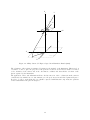
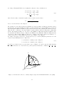
The direction based pointing is controlling the instrument based on target identified and located by a
sensor. The location of the sensor and instrument are generally different, and therefore setting the azimuth
and elevation angle from the sensor points the instrument at a different location. This problem is shown in
Figures 5.4 and 5.5. The figures are done on large scale to illustrate the effect of the displacement in both
azimuth and elevation angles, the system is not intended to be used with such large spatial displacements
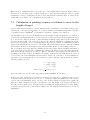
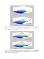
between instruments and sensor.
One can easily see that an algorithm is needed to determine the direction of pointing for the instrument,
based on the direction identified at the sensor. This algorithm shall take into consideration the place of
the instrument and the sensor.
Figure 5.4: Top view illustration of the system, showing effect of spatial displacement between the instrument and sensor: for different locations the azimuth angle (ω) that points towards the same target is
different.
Figure 5.5: Illustration of the system from the side, showing effect of spatial displacement between the
instrument and sensor: for different locations the elevation angle (γ) that points towards the same target
is different.
30
Then the steps for the direction based pointing control are the following:
1. Calculate vector between instrument and target in IWRF, based on the vector from the sensor.
2. Represent the same vector in PSRF.
3. Transform the representation of the vector from Cartesian coordinates to spherical coordinates.
Steps 2 and 3 have already been covered in the previous section, describing geo-pointing (see Sections 5.1.2
and 5.1.3 ).
5.2.1
Calculating the vector from the instrument to the target
To calculate the direction of pointing for the instrument we shall know the vector from the sensor to the
target and the vector between the sensor and instrument. Knowing them, both represented in the same
reference frame, the vector between the instrument and the target can be determined by subtraction.
The vector between sensor and instrument is calculated in SWRF with the method used in geo-pointing,
based on geodetic locations. The vector from sensor to target is determined based on data acquired by the
sensor, in SWRF. However in some cases this data contains the azimuth and elevation of the target, but
not its range. Therefore sometimes only the direction of the vector is known, not its magnitude.
To calculate the direction of the vector, let’s consider a unit vector v, as shown in picture Figure 5.6,
defined by the angles azimuth (ω) and elevation (γ). The components x (ni ) ,y (ei ) and z (ui ) are sought,
supposing that |v| = 1.
Z
Pi
v
γ
z(ui )
X
ω
y(ei )
p
Y
x(ni )
Figure 5.6: Calculating the components (x or ni , y or ei , z or ui ) of a vector (v) defined by azimuth (ω)
and elevation (γ).
Considering Figure 5.6 the following equations can be written:
z
p
, cos(γ) = ,
v
v
y
x
sin(ω) = , cos(ω) = ,
p
p
v = 1,
sin(γ) =
(5.11)
where p is the projection of vector v in the XY plane. Based on the expressions in Equation (5.11), the
equations expressing the components of the unit vector are the following:
ni = x = cos(ω) · cos(γ),
ei = y = sin(ω) · cos(γ),
(5.12)
ui = z = sin(γ).
Returning to the problem of the vector magnitude, the two control applications offer different targets.
In the case of the SvalTrack II software the targets are celestial bodies and satellites. In the case of the
31
satellites, based on the orbital data, the range of the vector from instrument to target can be calculated. As
for the celestial bodies, due to their large distance from Earth and due to the relatively very short distance
between instrument and sensor, it can be safely assumed that they are infinitely far away, and parallel
pointing is sufficient. Therefore the same azimuth and elevation are set on the instrument as given by the
sensor. It shall be noted that in this case, to minimize error, the geodetic position of the software shall be
set to either the exact same coordinates as the instrument, in the case of one controlled instrument, or in
the centre of the formation in case of multiple instruments.
For targets such as the aurora the height determination is more complicated (see Appendix C ), nevertheless
possible. However, as it is very probable to do only a rough estimation of it for simplifying the software
usage, Section 7.1 is dedicated to calculate the effect of a wrong estimation on the pointing accuracy.
Once the height of the target has been identified, the magnitude of the vector pointing from the sensor to
the target shall be calculated. The problem is illustrated in Figure 5.7.
T
S
γ
F
α
O
Figure 5.7: Calculating the magnitude of vector based on the height of the target. The lengths are not to
scale for the purpose of better illustration of the problem.
In Figure 5.7 ST is the length sought, TF is the height of the target and the angle marked with γ is
the elevation angle identified by the sensor. Since the geodetic location of the target is not possible to
identify, the radius of curvature in prime vertical cannot be calculated. Therefore to minimise the error
induced the following calculation has been made: considering that the aurora visible at KHO is the one
appearing between the latitudes of 65.961◦ and 82.136◦ (values from the program SvalTrack II), the radius
of curvature in prime vertical for those values is calculated and their mean value (6385992.9039 m) is used
for the lengths of OS and OF. This results in assuming a sphere instead of an ellipsoid that further simplifies
the calculations by the relation α = γ + 90◦ . The final equation for the vector magnitude therefore is:
ST = OS · cos(α) +
p
OT 2 − OS 2 · sin2 (α)
32
(5.13)
Chapter 6
Calibration
For the correct functioning of the system each unit playing active role in SvalPoint shall be calibrated. The
following information shall be acquired about each of them:
geodetic location (latitude, longitude and altitude),
home attitude in Tait-Bryan angles (roll, pitch and yaw).
In addition to these values it must be ensured that the sensors provide correct data, hence all their parts
contributing to target location is calibrated. The scientific data from the instruments does not play active
part in the pointing system, therefore their calibration is not a part of the SvalPoint calibration process.
6.1
Geodetic positioning of the instruments and sensors
The positioning of the instruments is done by Differential GPS (DGPS) measurements for the centre of the
instrument domes. Since all positions in the software are required in geodetic coordinates and the DGPS
measurements are performed in UTM system, transformation from it into geodetic coordinates is required.
See more information about the UTM in Appendix D.
6.1.1
Differential GPS
Differential GPS or DGPS is an enhancement to the Global Positioning System that increases the location
accuracy up to 10 cm in contrast to the approximately 8 m accuracy of GPS in normal operating conditions.
See also National Coordination Office for Space-Based Positioning (2014).
DGPS is based on computation and correction of range error for each GPS satellite in the view of a single
reference station, placed at a known location. In the case of Svalbard these locations are marked by a
concrete platform with a metallic bullet in its centre. Then the corrections are transmitted to the nearby
users, improving the accuracy of the measurements made by them. It shall be noted however, that as
the distance between reference station and user increases, the lines of sight through the ionosphere and
troposphere changes, resulting accuracy degradation as the delay to the station and user are different.
See Figure 6.1 for photos of the measurement process on sight.
6.1.2
The measurements
®
The formulas that transform from Transverse Mercator Projection into geodetic coordinates are named the
inverse Gauss-Krüger projection. To perform the transformation a MATLAB function is used from the
toolbox Wasmeier (2006). The function is named utm2ell, denoting transformation from UTM to ellipsoidal coordinates, taking into consideration the irregular sections (see Appendix D for more information
about the irregular sections). In the input there is an option of entering the standard for the ellipsoid, that
is implemented in the same toolbox as data structures. The DGPS measurements are done in ETRS89
33
Figure 6.1: Panel A: The DGPS station placed over the marked location in Svalbard, nearby KHO. Panel B:
The centre of each dome on the roof of the observatory is measured with the user equipment communicating
with the DGPS reference station.
that uses the GRS1980 ellipsoid, therefore that is the standard used for this transformation.
Each dome has been numbered and measured during the process. The measurements of the domes of interest in this project are the ones housing the Narrow Field of view sCMOS camera (referenced as Keo in the
followings), the Fs-Ikea and the all-sky camera - PTU D46 unit pair. See the values and their equivalent
in Geodetic coordinates in Table 6.1.
Note: This value represents the centre of the dome. For the centre of the instrument lens further spacial
offset measurements shall be done.
Due to delays in the delivery of the measurement data all tests of the system has been done based on data
acquired with a hand-held high precision GPS device available at KHO. Table 6.2 shows the values for
each instrument. These measurements have also served as a verification on the transformation results.
In conclusion the measurements are fairly consistent between the DGPS and hand-held GPS methods. The
largest error is for the Fs-Ikea instrument East coordinate, however it is fairly straightforward from the
pattern of the values, the hand-held device measurement was of low accuracy.
It shall be noted, that the DGPS measurements may be further refined considering that all domes have
the same height, the difference in it coming from the position of the user device that might have been not
perfectly vertical at times or might have been placed not exactly in the centre of the domes. Calculating
the mean value of all heights (measured on all domes on the top of the observatory) the result is 523220 mm
(value used in the calculation of error for the measurements with the hand-held GPS device).
34
Table 6.1: DGPS measurements and their equivalent in geodetic coordinates.
Instrument
UTM coordinates
East (m)
Height
(mm)
8675070.729 523835.847
523470
8675068.108 523831.084
523455
8675062.921 523821.632
523161
North (m)
Keo
Fs-Ikea
PTU D46
Geodetic coordinates
North (◦ )
East (◦ )
Height
(mm)
78.14775385 16.03963733 523470
78.14773113 16.0394276
523455
78.14768616 16.03901141 523161
Table 6.2: Geodetic coordinates of instruments measured with hand-held GPS device.
Instrument
Keo
Geodetic coordinates
North (◦ )
East (◦ )
Height
(mm)
78.14776
16.0396075
520000
Fs-Ikea
78.1477
PTU D46
78.147686667 16.03900667
6.2
16.0389
520000
520000
North (◦ ,m)
Error
East (◦ ,m)
0.00000615,
0.696
0.00003113,
12.034
0.000000507,
0.11
0.00002983,
0.674
0.0005276,
3.688
0.00000474,
0.054
Height
(mm)
322000
322000
322000
Home attitude determination of the instruments and sensors
For the calibration of the pitch and roll angles there is dedicated equipment available, a high precision
level. For the yaw calibration however the geo-pointing is used.
It shall be noted early on that as the coordinate systems used are left handed the sign of the angles is
as follows: yaw angle is positive from North towards East, pitch angle is positive in the direction from
horizontal to down, and roll is positive in the direction from right to left.
6.2.1
Yaw calibration
To define the yaw the offset from North shall be determined. The Geo-pointing is used for this procedure.
Assuming that the location of the instrument is correctly determined and that the pitch and roll angles are
correctly measured, by pointing at known locations the yaw angle input can be adjusted until the picked
points appear in the centre of the image taken by the instrument. The calibration points shall be picked
in a way that the features are easily recognised in the image, e.g. mountain tops or distinctive features of
the shore. The process shall be done for several points, followed by the calculation of a mean value for the
resulting yaw angles. In case the difference between the calibration points is unacceptably large (e.g. in
the order of 10-1 ◦ ), the location, pitch and roll calibrations shall be revisited.
In the followings the calibration for the Tracker Camera is shown. It shall be noted that at the time of the
calibration only hand-held GPS measurements have been available about the location of the instruments.
The pitch and roll angles have been measured with a digital level as accurately as possible, resulting in the
values +0.4◦ , and +0.7◦ respectively. However, at later stages of testing it has turned out that these values
have not been precise enough. Moreover, at the time of the calibration there has been a mistake in the
code that limits the precision of the camera movement. These are the possible reasons for offset appearing
in pictures. Despite these problems the results for the yaw are fairly correct, as shown later, in Chapter 8.
Figure 6.2 shows the map of the target upon which the first calculation has been made. The yaw of the
instrument has been initially approximated to be -32◦ . Pictures of the target have been taken with different
settings for initial yaw, with the aim of finding the angle that results in the target being in the centre of
the image upon the execution of command. See Figure 6.3 for the images with -26◦ , -28◦ and -30◦ initial
yaw settings.
The second and third targets are chosen as shown in Figure 6.4 and Figure 6.5. As the targets are in the
centre of the pictures, no further adjustments are needed.
35
Figure 6.2: The first target of pointing for the yaw angle calibration, marked by the red circle. The green
arrow marks the direction of pointing. The map used in the image is the property of the Norwegian Polar
Institute. (Norwegian Polar Institute 2014)
Figure 6.3: Pictures taken of the first target (see fig. 6.2) during the yaw calibration in the order -26◦ , -28◦
and -30◦ for initial yaw. The target is marked with a red circle in each picture it is visible in.
36
Figure 6.4: The second calibration target: Adventstoppen. The centre of the image taken by the Tracker
Camera is marked by the orange cross, while the targets on both images are marked by the red circles.
The map in the image is the property of the Norwegian Polar Institute. (Norwegian Polar Institute 2014)
Figure 6.5: The third validation target: Hiorthhamn. The centre of the image taken by the Tracker Camera
is marked by the orange cross, while the targets on both images are marked by the red circles. The map
used in the image is the property of the Norwegian Polar Institute. (Norwegian Polar Institute 2014)
6.2.2
Pitch and Roll calibration
The roll and pitch can be measured with the use of a level on the instrument platform. The precision
required for the calibration is based on the accuracy of the motion for the instruments, as it shall not be
lower. The accuracy for both the Narrow Field of view sCMOS camera and the Fs-Ikea is ±0.05◦ , while
for instruments based on PTU D46 unit no accuracy is available however the resolution of motion is known
to be: 0.0129◦ . Based also on the availability of the digital levels, one with 0.01◦ resolution is chosen.
Furthermore the equipment is factory-calibrated, ensuring the most precise measurements possible.
In case the level is placed on the instrument platform it is assumed that the platform and the instrument
are perfectly aligned, inducing possible errors in the calibration. However, as the instrument rests on the
platform in the case of the Narrow Field of view sCMOS camera and the Fs-Ikea, this error is minimum.
Special attention shall be paid to the alignment of the level with the instrument. The level however has
37
very convenient flat surfaces on all sides therefore it can be easily aligned with the edges of the platform.
In both cases both the yaw and pitch error turned out to be 0.02◦ , indicating that perhaps these angles
are induced by the building itself.
In the case of the Tracker Camera and the all-sky camera however the assumption of their alignment with
the platform induces errors in the scale of entire degrees. This is due to the fact that the platform is
constructed of raw worked wood and metallic brackets fixed with screws. Moreover there is no space for
placing the level accurately. Therefore a different approach is taken for the measurements, that is similar
to the yaw calibration.
For the Tracker camera after making an initial measurement of the pitch and roll the camera is pointed
at different targets and with trial and error method the angles are adjusted until the target is in the
centre of the picture. However, as there are two angles to change and their effect on the pointing is not
straightforward, it is not an effective or very precise process. However, as the camera is not used for
gathering scientific information, the requirement for the precision of pointing is not that high. As long as
the target is in the picture it is considered satisfactory.
In the case of the all-sky camera the same approach is used, only that a calibrated instrument is pointed
by the use of the Sval-X Camera control interface. The angles are adjusted until the instrument records
images of the target selected in the sensor’s picture.
6.3
All-sky camera calibration
The lens of the all-sky camera is a Fujinon FE185C046HA-1 fish-eye lens. According to Fujinon Fujifilm
(2009) it has an equidistant projection (see Equation (2.4)), a focal length of 1.4 mm and a field of view
(FOV) of 185◦ . However, when these parameters are used the resulting FOV is over 200◦ .
In consequence two verifications are done for the lens: verification of the FOV, especially in the light of
Krishnan & Nayar (2008) stating that after calibration the FOV for this lens has been found to be 194◦ ,
and the equidistant projection equation is suspected to have a scaling factor that needs to be determined
(please refer to Section 2.2 for more details on the equidistant projection equation).
The calibration is done with a small light source mounted on an arm of 1 m, that is in turn mounted
on a tripod with a panning module showing the degrees of rotation. The alls-sky camera is fixed to a
platform and the following coordinate system is considered: the x axis coincides with the optical axis and
y is perpendicular to it in the centre of the lens. Plane xy is parallel with the plane of the arm’s movement.
The tripod is placed under the lens, aligning the centre of the rotation of the arm with the centre of the
lens as precisely as possible. The spatial offset is measured with the help of a pendulum and measuring
tape, giving an offset on the x axis of 0.75 cm, and 0 cm on the y axis. The levelling of the tripod and
camera platform has also been adjusted to the best possible, and measured with a high resolution (0.01◦ )
level. The measured offsets of the tripod are 0.57◦ around the y axis and 0.04◦ around the x axis, while the
same measures for the platform are 0.06◦ around y axis and 0.2◦ around x axis. The height of the tripod
is adjusted to have the light source shining exactly at the middle of the lens, adjustment made using the
pictures captured by the camera.
To calculate the FOV the arm is rotated around to the point when the light source disappears on the
horizons. On both sides the angle value on the panning module is read. From these values not only the
FOV but also the angle value at the middle of the lens is determined.
To determine the projection equation for the lens images are recorded with 640×512 pixels resolution while
turning the arm from the centre towards the horizons with 10◦ steps, except for when the source reaches
the horizon, that step is only 7.5◦ . The process is repeated two times to compensate for adjustment errors,
and the values are averaged. All angle values measured are adjusted according to the 0.75 cm spatial offset
of the rotation point of the tripod from the centre of the lens.
Figure 6.6 shows some of the calibration images for the fish-eye lens. The images start with the light source
in the centre (image A), then it moves towards the left horizon. Image B is taken with the light source
moved 10◦ to the left. Images C and D are the last two steps: right before and on the horizon.
38
Figure 6.6: Examples for images recorded during the calibration of the fish-eye lens (note: the images are
colour-inverted). The light source is marked with a red circle in each picture.
39
6.3.1
Compensation for spatial displacement
Figure 6.7 is a sketch of the calibration equipment set-up: the centre of the lens is placed in point O, the
rotational axis of the tripod is placed in point B. The light source is in point C, moved there from point A.
It is clearly visible that the angle displacement read from the panning module of the tripod (α) is different
from the angle displacement for the lens (β), the two angles having the relationship α > β.
A
α
B
β
O
C
Figure 6.7: Top view of the calibration set-up. Illustration of the effect of a spatial offset of the rotational
axis of the arm and the centre of the camera (OB) on axis x of the lens calibration system.
To calculate β we consider the triangle 4BOC, as in Figure 6.8. In this triangle the lengths CB and OB
are known: CB is the length of the arm and OB is the displacement on axis x in the system. Also, note
that from Figure 6.7 angle α is the measured angle on the panning unit of the tripod.
O
β
C
α0
γ
B
D
Figure 6.8: Calculating the angle for the fish-eye lens based on the angle measured in the calibration
system. 4BOC.
The relations in 4BOC are:
α0 = 180◦ − α,
OD
,
sin(α0 ) =
OB
DB
cos(α0 ) =
,
OB
OD
sin(γ) =
,
OC
CD
cos(γ) =
,
OC
CD + DB = CB,
α0 + β + γ = 180◦ .
40
(6.1)
From Equation (6.1) follows
OD = OB · sin(α0 ),
DB = OB · cos(α0 )
(6.2)
and
CD = CB − DB,
(6.3)
CD2
OD2
+
= 1.
2
OC
OC 2
Based on the trigonometric equation sin2 (γ) + cos2 (γ) = 1:
p
OC = OD2 + CD2 .
(6.4)
Therefore:
γ = arcsin
OD
OC
◦
,
(6.5)
0
β = 180 − γ − α .
6.3.2
The measurements
The measurements, considering the angle adjustments show that the horizon is on 97◦ from the centre,
resulting in a FOV of 194◦ , the same as the value found in Krishnan & Nayar (2008).
To calculate the projection equation the pictures taken with 10◦ steps has been analysed. On the pictures
the light source represents approximately 3 pixels in width and 3 pixels in height. Therefore the central
pixel has been used to determine the place of the light source, in a 2-axis Cartesian coordinate system (x
and y) on the picture. Knowing the centre of the picture the distance of the light source from it in pixels
can be determined.
The pixel size of the DDC1240C-HQ camera used in the mount is 5.3µm × 5.3µm (see Thorlabs (2011)),
and knowing that the full resolution of the camera is 1280 × 1024, while the recorded image is in 640 × 512
resolution, the distance from the centre can be determined.
Assuming that the projection is equidistant and only a scaling factor is unknown then the following equation
can be written:
r = fe · θ,
fe = a · f,
(6.6)
where r is the distance of point from the centre of image, fe is the effective focal length, f is the focal
length, θ is the angle between optical axis and the incoming ray in radians and a is the scaling factor.
Using the angles measured, then adjusted, and the distance of the source determined from the images
an fe for each angle can be calculated. Calculating the mean value for the effective focal length gives
fe = 1.42463427mm, resulting in a = 1.017595907.
The largest difference between two fe values is 0.0157 mm, therefore it can be concluded that the projection
is indeed equidistant.
Note: these values apply for the specific all-sky camera with the used sensor, as the sensor has not been
previously calibrated on its own.
41
Chapter 7
The accuracy of pointing
The system is planned to be used for various observations, for various targets, the main focus being aurora.
Due to the very dynamic nature of the phenomenon and the large variety of its shape, size and location in
the sky, also due to the differing nature of scientific observations there could not be a well defined accuracy
requirement from the start, ultimately aiming for having the target in the field of view of the instrument.
The system involves many processes that contain both human factor and a multitude of possibly standing
cases contributing to the accuracy of pointing, noting that errors may propagate ultimately and they shall
be reduced as much as possible in all cases. Therefore the problem is discussed in terms of absolute limitations and conditions that change the final accuracy.
The first and most important factor in the accuracy is the resolution of the pointing control motors. This
limits the finery of the motion, and therefore sets an absolute technical limit on the accuracy of the pointing. The values for the different instruments are to be found in Chapter 3.
On the other hand, since the instruments are not sensing with a single pixel, but have a field of view, some
displacement may be permitted, considering the size of the target and nature of observation, as the image
acquired might still contain the target. One can draw the conclusion that chance for the success of the
pointing decreases with the increase in the size of the target.
The second large factor limiting the accuracy to be considered is the pointing algorithms of the instruments.
Three major limitations shall be considered: calibration inaccuracies, the accuracy in the target location
and the accuracy of target identification.
The inaccuracy in the initial instrument attitude (coming from calibration errors) affects all modes of
instrument control. When transforming the vector from its representation in the Instrument World Reference Frame (IWRF) to a representation in the Pointing System Reference Frame (PSRF), as the PSRF is
calculated by the roll, pitch and yaw angles, the direction will be offset with as much as the error in these
angles. This results in effects and further discussion identical to the motion resolution problem, presented
earlier.
In the case of geo-pointing, considering that the positioning of the instrument and target is exact, the
pointing is more accurate than the resolution of the motors, limited only by the accuracy of real number
representation in the computer. The source of inaccuracy lies in the exact positioning of both instrument
and target. Considering inaccurate acquisition of location data for target and/or instrument, the direction
of pointing will experience larger error at shorter instrument-target distances.
In the case of direction based pointing location calibration errors for the sensor and instrument introduce a
decrease in accuracy that is also more visible at close targets. This method has however further limitations
to consider. In the case of the Sval-X Camera, when an all-sky camera is used for target location and no
information can be acquired about the range of the target, the correctness of the height estimation limits
the accuracy. See more about it and its effects in Subsection 7.1. Furthermore, calculating the range based
on the height of target is done with an estimated curvature in prime vertical of the ellipsoid that reduces
the accuracy of the calculations. The effect of this is the smallest when the target is at 90◦ elevation angle.
42
Errors in target identification may occur in the case of the Sval-X Camera, when an all-sky camera is
used for sensor. The image often reveals less details close to the horizon, increasing the chance for wrong
identification of target. Considering the aurora, supposing that its horizontal feature is of interest, its
details will be more visible close to zenith than at low elevations.
7.1
Calculation of pointing accuracy in relation to error in the
height of target
As previously discussed in Chapter 5 and in this chapter the determination of the height of target is necessary in case of direction based pointing. To be able to estimate and visualize its importance and effect
on pointing accuracy a MATLAB program has been written, consisting of two functions.
®
The first function gives the error in azimuth and elevation angles. It takes as inputs the vector direction
between sensor and instrument, the vector direction between target and sensor and the height of the target
above the reference ellipsoid (an array of different heights). It has fixed the height set in the SvalPoint for
the target and the height of the sensor above the reference ellipsoid. The function calculates the magnitude for the sensor-target vector for each height input, followed by the calculation of azimuth and elevation
angles for the instrument-target vector for each height. Then, subtracting from these values the azimuth
and elevation calculated for the height of target set in the SvalPoint the error in pointing is achieved.
The second function generates different possibilities and plots the graphs. The plots shall show the function
between the angle error (separately for azimuth and elevation), the distance between the sensor and instrument and the height of target above reference ellipsoid. The hard-coded parameters in this function are
the limits for the height of target, the limits for the distance between sensor and instrument, the direction
vectors both for the sensor-instrument and sensor-target. In the case of the latter one all possibilities are
investigated by generating all unit vectors on quarter of a sphere with the origin in (0,0,0). For this the
following equations are used:
x = cos(θ) · sin(ϕ),
y = sin(θ) · sin(ϕ),
z = cos(ϕ),
π
where: 0 ≤ θ ≤ and 0 ≤ ϕ ≤ π.
2
(7.1)
Out of the angle errors for all possible target directions the maximum error is chosen.
Both most probable and worst case scenarios are investigated for being able to estimate the affect of error
on system accuracy. The height of sensor is set to be 520 m, the height of the KHO station. The distance
between sensor and instrument varies between 0 to 22.5 m, these distances being the most realistic estimations for future situations: the span of 10 adjacent rooms. The height of the target is calculated for
the values 70 and 550 km, based on Strømer (1955), presenting the height distribution of a large number
of auroral observations between 1911-1944 (See Figure 7.1). The height measurements have been done by
triangulation.
43
Figure 7.1: The distribution of auroral heights in Strømer (1955). The plot shows the number of events on
axis x versus the height of the occurrences. Image adapted from Brekke (2012).
First the worst case calculations are presented, with the sensor-instrument direction vectors being: (1,0,0),
(0,1,0) and (0,0,1) in North-East-Up coordinates. See Figure 7.3 and Figure 7.2 for the results. Based
on these images one can see that the best configuration for sensor and instrument would be to be atop of
each-other (Figure 7.3), however that is physically impossible due to view-field problems. One can draw the
conclusion that if the sensors are at the same level further errors in elevation are eliminated. Furthermore,
the placement of sensors in the North-East plane do not make any difference. The maximum error in angles
are 0.4714◦ for azimuth and 0.0094◦ for elevation. These are worst case scenarios, without any attempt of
determining the height of the aurora, having a constant 110 km set (the most frequent height of aurora
according to Kaila (1987) and Figure 7.1).
Considering a more realistic scenario, the sensor and instrument are placed at ( √12 , √12 , 0) direction. Note
that the North-East coordinates do not make difference, as concluded earlier, however they are levelled
for the best possible results. The height of target is determined to be 200 km with 50 km uncertainty.
For the graph in Figure 7.4 the height of the target set in the SvalPoint is 200 km, resulting in the errors
0.1081◦ in azimuth and 0.0022·e-4 ◦ in elevation. As one may see, the error in pointing is larger if the
44
target is lower than the estimated height, therefore one may conclude that performance may be maximized
if a lower value is entered for the height in the SvalPoint system, to balance the errors. It has been found
that in this case the value 187 km is the height of target value that results in the lowest error in pointing
for the 150 - 250 km range: 0.0873◦ in azimuth and 0.0017·e− 4◦ in elevation. See Figure 7.5.
Figure 7.2: The resulting error for azimuth and elevation angles in the function of height of target and
distance between sensor and instrument if the direction of instrument is the (1,0,0) or (0,1,0) unit vector
from sensor and the set value in SvalPoint for the height of target is 110 km. The maximum value for
azimuth and elevation errors are 0.4714◦ and 0.0094◦ . Graph plotted with MATLAB .
®
Figure 7.3: The resulting error elevation angle in the function of height of target and distance between
sensor and instrument if the direction of instrument is the (0,0,1) unit vector from sensor and the set value
in SvalPoint for the height of target is 110 km. The maximum value for azimuth and elevation errors are
2.5444·e-14 ◦ (approximately 0◦ ) and 0.0047◦ . Graph plotted with MATLAB .
®
45
Figure 7.4: The resulting error for azimuth and elevation angles in the function of height of target and
distance between sensor and instrument with the height of target 200 km, estimated with 50 km uncertainty.
Height set in SvalPoint: 200 km. The maximum value for azimuth and elevation errors are 0.1081◦ and
0.0022◦ . Graph plotted with MATLAB .
®
Figure 7.5: The resulting error for azimuth and elevation angles in the function of height of target and
distance between sensor and instrument with the height of target 200 km, estimated with 50 km uncertainty.
Height set in SvalPoint: 187 km. The maximum value for azimuth and elevation errors are 0.0873◦ and
0.0017◦ . Graph plotted with MATLAB .
®
46
Chapter 8
Validation
The complete validation of the system includes the testing of the connections and the testing of the pointing
itself. It is done in order to ensure that the system can be used to perform the tasks that it was designed
for, fulfilling all aims of the project.
8.1
Validation plan
For validating that the SvalPoint system is working from the connection’s point of view the following tests
shall be done:
1. connect to all combinations of the possible servers (e.g. connect to Fs-Ikea Tracker, and Keo Sky
Scanner but not the PTU46 Tracker), making sure that they respond correctly,
2. try connection with the firewall blocking all attempts to connect, then from a computer that is not
in the exception list, making sure that the connection is declined in both cases,
3. connect and disconnect repeatedly with the client application, making sure that new connection is
possible after each disconnection,
4. try connecting the client to servers that are not connected to the internet, making sure that the
failure to connect is properly indicated in the client,
5. and finally attempt connection to several servers, some of them connected to the internet, others not,
making sure that the ones connected react to the commands, while for the disconnected ones the lack
of connection is indicated.
Each control possibility with all interfaces shall be validated. During the tests all instruments shall be
pointed, and the data collected shall be analysed to confirm that the target was indeed acquired.
1. pointing at geographical features identified in a map, using geo-pointing, making sure that each target
is found in the centre of the pictures,
2. pointing at targets identified in the sensor, covering both targets close to the horizon and at zenith
position, making sure that all instruments acquire the same target,
3. pointing at auroral structures, making sure that the acquired target is consistent for all instruments,
but also assessing the speed of the operation of SvalPoint versus the dynamics of the aurora,
4. tracking the moon with all instruments, making sure that the target stays in the field of view of the
instruments after an extended time,
5. tracking of stars with instruments, verifying that the targets are not lost after extended time,
6. tracking of satellites shall be done on a selection that are visible in the night sky and it shall be
verified that the instruments keep the satellite in their field of view during its visibility above the
horizon.
47
8.2
Performed validation
SvalPoint has been validated entirely from the connection’s point of view and all tests have passed. The
validation of the pointing on the other hand has been performed only partially. This is due to both the
light conditions in the time frame in which the thesis work took place and for a technical failure on site
that has not been solved in the time limit. One of the motor controllers on the Fs-Ikea instrument have
failed, therefore its pointing could not be tested; textual output about the control angles has been verified
in its case. The other reason for the partial validation is that dark sky returns in September (a time until
which this project does not extend), therefore stars, satellites and the aurora are not visible. Also, at the
time of the validation there was no suitable time for testing on the moon as it has always been very close
to the horizon. Until the present moment test 1 and a part of test 2 has been conducted.
Test 1. Due to the mathematical nature of the method, the geo-pointing is the most accurate pointing and
the test associated to it is rather a validation of the calibration values than of the method (the geo-pointing
is also actively used in the calibration, see Chapter 6 ). Actual test on the method were done only in order
to make sure that all formulas are correct in the program. This has been done by approximative pointing
at a number of different targets. The targets chosen have been geographical features, easily identifiable
from a picture, such as mountain tops and features of the sea-shore. The determination of their geodetic
coordinates and height has been done based on the maps provided by the Norwegian Polar Institute (Norwegian Polar Institute 2014).
Test 2. The pointing methods based on the all-sky camera have been tested after calibration.
The testing equipment is the following: the Tracker Camera (instrument 1) placed at approximately 30 cm
distance from the alls-sky camera (sensor), both of them being located in the same dome; and the Narrow
Field of view sCMOS camera (instrument 2) located at 5 m distance from the sensor, two rooms away. The
chosen target is a mountain showing on the horizon, for which due to its proximity the system is expected
to perform worse than for the primary target.
It shall be noted that the tests have been conducted with a fixed 110 km height of target. This induces for
the Narrow Field of view sCMOS camera a maximum error of 0.2629◦ in azimuth and 0.007◦ in elevation,
however in the specific scenario it is much smaller: 0◦ in azimuth and 0.0104◦ in elevation, according
to mathematical calculations similar to the ones presented in Section 7.1. The Tracker Camera being at
approximately 30 cm distance from the sensor, is not affected by this error: the first noticeable difference
(0.05◦ , the pointing accuracy of the instruments) appears at 75 cm distance from the sensor (in case of a
1 km target altitude, the approximate height of the surrounding mountains), calculated with MATLAB
similarly to the calculations in Section 7.1.
The pictures recorded during this test are shown in Figure 8.1. The total error in pointing is the angle
between the optical axis and vector to the target from the centre of the instrument lens. For the Tracker
Camera this is 0.7725◦ whilst for the Narrow Field of view sCMOS camera it is 0.0259◦ .
®
As one might notice in Figure 8.1, the target on the all-sky camera is at a very low elevation angle, appearing as just a few pixels on the image, with barely identifiable features. Indeed, after selecting the target
on the picture usually naked eye test has also been preformed to see better how does the feature look like
and hence be able to identify it on the images acquired by the instruments. The erroneous identification
of targets shall induce the same magnitude error in all instruments: an offset from the intended target of
pointing.
Considering the fact that the two instruments have different error in pointing, an error not justified by
wrong target selection and larger in case of the Tracker Camera, further error sources shall be considered.
The most probable cause is identified to be calibration error in the initial attitude measurements. As
described in Chapter 6 the calibration method has been different and more inaccurate for the Tracker
Camera, that took the second image in Figure 8.1.
As mentioned in the same chapter, at the time of the calibration there has also been a rounding mistake in
the geo-pointing feature of the software, used as the basis of the calibration, that has limited the accuracy
of the pointing, effecting the initial yaw measurement on both instruments. In conclusion the calibration
48
Figure 8.1: Images taken during the validation of the system. The images are recorded as follows (from left
to right): image from the all-sky camera, as sensor, the red cross in the yellow circle marking the target
of pointing; image recorded by the Tracking Camera; image acquired by the Narrow Field of view sCMOS
camera (image upside down and mirrored due to the reflections in the flat surface mirror assembly). On
both images acquired by the instruments the orange cross marks the centre, the blue lines mark the centre
of the image from the other camera and the red circle marks the target of pointing.
values have been more inaccurate in this instance then they will be in the future. However, as the Tracker
Camera unit is not an instrument of interest but has been used only for testing, and the target is still in
the field of view, and since the Narrow Field of view sCMOS camera has a pointing accuracy considered
satisfactory, the re-calibration has not been done, and the test has been considered passed.
Summarizing the sources of errors in both units, the following factors are relevant, in decreasing order of
their estimated magnitude:
Narrow Field of view sCMOS camera
– yaw calibration error,
– height of target error,
– target identification error;
Tracker Camera
– roll, pitch and yaw calibration error,
– target identification error.
49
Chapter 9
Conclusions
The system developed during this thesis enables a large range of scientific observations. Some of the observations that can be done for the first time at KHO are: multiple instruments pointing at the same target,
acquiring different data in their nature complementing each other, the same target can be observed by a
satellite performing in-situ measurements and ground station with the satellite tracking feature. Also, for
the first time at the observatory target acquisition became very intuitive and easily done. However, most
importantly this system has accomplished the control of the instruments over the internet, opening up a
wide range of possibilities for future development, representing their corner-stone.
The current version of SvalPoint consists of 6 software applications categorized as follows by their role in
the system: server, client and control interface. Each instrument is associated with a server application,
running on its control computer controlling the instruments, commanded through the client with data
about the target from one of the control interfaces. The control interface applications had already been
developed at the start of the thesis and only minor changes have been required in them. The client and
the server applications have been implemented during the time-span of the thesis work.
Due to the complexity of the system a User’s Manual provided that introduces the reader to the system,
compiling all information needed for the use of the software package and to support the future maintainer
of SvalPoint. See Appendix E for fragments of the user manual.
The current system is capable of pointing 4 instruments installed at KHO at the same time, counting the
test instrument used for development not installed on a fixed platform. The instruments may be picked in
any combination, and only the selected ones are commanded. The scientific data collection is not part of
the system, standalone programs are developed for them.
The theoretical accuracy of SvalPoint is limited only by the motion accuracy of the individual instruments.
However, in practice the following factors influence the pointing accuracy: precision of calibration, human
factor at the selection of target in the control interface and the accuracy of the target’s height determination.
During the time of the thesis only partial validation has been possible due to light conditions and technical
difficulties at KHO. The complete validation and trial of the competence of the system for the required
observations is to be done in the up-coming auroral season. After the first observations the ease of use
for the system is to be assessed and modifications may be done to the user interface or software interactions.
One of the most important features of the system is that its design leaves room for further development.
After the real test of the system new programs may be developed, especially on the client side, for target identification. Features such as image processing for the automatic identification of aurora, and the
scanning of its entire area, or the mounting of instruments or sensors on truck, aircraft or other moving
platforms, with sensors to determine their changing attitude or mobile phone application based remote
control are all possible to be developed. Also, further sensors or instruments may be added with little
effort, placed at very different locations, extending all the way to the mainland.
50
Further helpful software applications for making the use of SvalPoint easier would be the ones that help
calculating the height of the target and determining the value that shall be the input for the system. As
discussed in Appendix C the determination of the height of aurora is a complex problem in itself, therefore
to be able to do it at a time-scale suitable for the observations an automated software is absolutely necessary.
Furthermore, as shown in Section 7.1 when the height is estimated with a given uncertainty, in order to
have the smallest possible errors a different value shall be entered in the system than the estimation. This
value can be calculated for each estimation, therefore an option for it in the control interface would further
enhance accuracy without causing the operation to be significantly more complicated.
51
Appendix A
The Kjell Henriksen Observatory
Figures A.1, A.2 and A.3 show details of the KHO building. The pictures are presented to help the better
understanding of the need for the system and the motivation for different aims and desired features of
SvalPoint.
Figure A.1: Basic design of the observatory with a drawing of the standard instrument module. Image
from KHO (2014d).
52
Figure A.2: Fragment of the map of KHO showing allocation of instruments with the focus on the facilities
located in the service section of the building. Note the operational room marked with ’operasjonsrom’.
Image from KHO (2014d).
53
Figure A.3: Photos taken at KHO showing the domes on the roof, housing the instruments, the building
with the road leading to it, and the corridor of the instrumental wing with the instrument modules on
both sides.
54
Appendix B
Tait-Bryan angles
The Tait-Bryan angles, also named as asymmetrical Euler angle sets or 3-2-1 Euler angles, represent
rotations around three distinct axes: x, y and z. The angles are named roll, pitch and yaw, and in the case
of a ship or aircraft they are defined as follows (Berlin 2007):
roll is the rocking movement around the longitudinal axis, in general rotation around axis x,
pitch is the up-down movement of the longitudinal axis, in general rotation around axis y,
and yaw is the sideways movement of the longitudinal axis, in general rotation around axis z.
In the case of an aircraft Figure B.1a illustrates the three angles. The same angles are adapted for the
different reference frames associated with optical instruments: the rotations around the axes follow the
convention described. For a left handed reference frame placed in the centre of the lens see Figure B.1b.
(a) The principal axes of an aircraft. (Mahoney 2014)
(b) The principal axes of a camera.
Figure B.1: Illustration of the principal axes.
55
Appendix C
Calculation of the height of aurora
The determination of the height of aurora is an issue that has been studied since the 1950-s, yet still a
problem today, resulting in numerous scientific articles. The earliest studies use triangulation in general
based on different cameras (narrow field of view, all-sky), with a spatial displacement from 4 to 100 km.
An early study of auroral heights is done in Strømer (1955), using narrow field of view camera photography
placed at distances of only a couple of kilometres, calculating the altitude of a single point in the auroral
arc. Studies on the determination of the height and position of the aurora based on a single sensor has been
conducted in Rees (1963) followed by Dandekar (1974) further improving the method. Kaila (1987) shows a
method for determining the height along the entire auroral form with a ±1 km precision if certain criterion
are met, using two all-sky cameras placed at 100-200 km apart from each other. More recent articles on
the subject are Sigernes et al. (1996) determining the height of midmorning aurora with photometers and
Whiter et al. (2013), presenting a method for finding the peak emission height of the aurora based on a
pair of all-sky camera images, bringing improvement in speed, accuracy and level of automation compared
to the earlier works.
The presented methods for locating the place of aurora involve visual or photometric data. However, due to
the nature of the phenomenon other measurements can be used as well by understanding the basic process
of the aurora.
The cause of the aurora is protons and electrons accelerated at thousands of kilometres height. The large
flux of electrons moving downwards into the ionosphere (called electron precipitation) collide with atoms
and molecules, getting them in an excited state. The excess energy during the de-excitation creates optical
emission (auroral arcs) and increases conductivity by creating secondary charged particles. The optical
emission and conductivity profiles are strongly dependent on the flux and energy spectrum of the precipitating electrons. Therefore models can be used to determine the height of the aurora (among other
parameters) in case information about the precipitating electrons is available.
To determine these parameters different approaches may be used. One approach is to collect in-situ data
from satellites or sounding rocket measurements. An example for the latter one presented in Sharp et al.
(1979), showing height distribution of emission rates, ion densities, auroral electron densities and flux.
One of the EISCAT radars, located in close vicinity of KHO can also be used to determine the height.
EISCAT determines the height distribution of the electron density and electron temperature among its
four basic parameters. These parameters can be also combined with optical observations making complex
observations possible. In Frey et al. (1998) a three dimensional model of the auroral emission is constructed
with the use of optical tomography and EISCAT data.
In conclusion, after presenting different methods and options for determining the heigh of the aurora it
shall be noted that all these observations are complex, therefore take time, possibly not comparable with
the dynamics of the phenomena. In case any of the options is to be used, a well automated process is at
need.
On the other hand, depending on the precision needed for the observations a fairly good guess about the
height might be sufficient. See the induced angle errors by imprecision in height in Section 7.1.
56
Appendix D
Universal Transverse Mercator
coordinate system
The Universal Transverse Mercator (UTM) coordinate system uses two-dimensional Cartesian coordinates
to define locations on the surface of Earth. It is the preferred system for large scale mapping (1:250000
and larger scales), giving the advantage of simple numbers over the complex degrees, minutes and seconds
of latitude and longitude. For more details consult Terry Jr (1996).
As described in Hager et al. (1992) as well the Mercator Projection can be visualised as an ellipsoid projected
into a cylinder, tangent at the equator and the polar axis coinciding with the axis of the cylinder. Opening
and flattening the cylinder results in distortion at the polar regions, while the showing true distances along
the Equator.
The Transverse Mercator Projection is a Mercator Projection with the cylinder rotated by 90◦ , resulting
in the ellipsoid and cylinder being tangent along a meridian. In this case when the cylinder is flattened
the east and west extremities appear distorted, however there is no distortion along the meridian that is
tangent to the cylinder, showing true distances. The zone around the meridian considered still sufficiently
little distorted is 3◦ in each direction, resulting in 6◦ wide portions for the system, dividing the Earth in
60 longitudinal mapping zones. See also Hager et al. (1992).
Figure D.1: Illustration of the UTM. CM - Central Meridian; AB, DE - Lines of secancy formed by the
intersection of cylinder and ellipsoid. Image from Hager et al. (1992).
The Universal Mercator Projection modifies the cylinder of projection by reducing its elliptical dimensions
and making it secant to the ellipsoid. It results in intersecting the ellipsoid along lines parallel to the
central meridian. (See Figure D.1) In one 6◦ zone the lines of secancy establish approximately 180000 m
east and west from the central meridian. The effect of these lines of secancy is that of allowing a more
57
consistent relationship between ellipsoid and map distances, resulting in a scale factor of 0.9996 for the
conformal coordinates in the plane. (See Hofmann-Wellenhof et al. (2001), Hager et al. (1992).)
The grid zones are defined uniform over the globe, however as shown in Figure D.2 there are exceptions
to this rule in the Scandinavian region: the south-west coast of Norway and the area of Svalbard. Around
Svalbard there are four grid zones 31X, 33X, 35X and 37X are extended to widths of 9◦ , 12◦ , 12◦ and 9◦
respectively, reducing the number of zones from seven to four, resulting in the fact that the grid zones 32X,
34X and 36X are not in use.
Figure D.2: UTM grid zones in Scandinavia. Figure from Bernhardsen (1992).
58
Appendix E
Fragments from the user manual to
the SvalPoint system
Due to the complexity of the system a user manual is provided to it that contains practical information
for the operator of the system. It also describes the structure of the software and the algorithms used for
the developer maintaining and extending it. This appendix shows fragments of the user manual, showing
examples of the practical information included in it.
E.1
What is SvalPoint?
The SvalPoint system is a collection of software programs that control a number of optical instruments at
the Kjell Henriksen Observatory (KHO). The instruments are controlled with internet protocol, therefore
they can be controlled from the building of the University Centre in Svalbard (UNIS). It shall be noted
however that the Firewall settings in Windows on the computers at KHO do not allow access from other
than PC-s registered as part of the KHO network.
E.2
How to use SvalPoint?
On the computers connected directly to the instruments, at KHO, the server programs shall run: Fs Ikea
Tracker (for the Fs-Ikea instrument), KeoSkyScanner (for the Narrow Field of view sCMOS camera)
and PTU46 Tracker (for any instrument fixed on PTU D46 platform). The server applications are ought
to be installed already on the computers. In case they are not, copy the folder of each server directly to
the C: (in case of the PTU46 Tracker and KeoSkyScanner) and to the D: directory (in the case of the Fs
Ikea Tracker).
When the programs are launched they look as in Figure E.1. Verify the IP address of the computer, also
note the Port. The same Port number shall be used in the client applications. After all parameters are
set correctly, connect it to the internet by clicking the ’Connect to Internet’ button. If continuous logging
is not desired, remove the tick from the check-box. In that case you can save the content of the dialogue
window by clicking ’Save log’. For emptying the log file click ’Clear Log’. The log file can be accessed in
the directory of the program. The files are named FS IKEAScanner log.txt, KeoSkyScanner log.txt, and
PTU46Tracker log.txt for the three different instruments.
Also make sure that the COM-ports are set correctly for the instruments, being one of the most common
troubles. Access it through the ’Settings’ tab, then ’Port Settings’. Verify the rest of the settings through
the other tabs. Use the ’Help’ tabs for more information.
The second part of the system is the client. That can be launched on any computer registered as part of
the KHO network. The software is named SvalCast. Launch it and select the instruments from the list
that you wish to control, then click ’Connect’. Feedback from the servers appear in the ’Info’ field. If the
59
Figure E.1: The user interface of the server applications.
IP address or Port number is incorrect, edit them in the Tracker Console Clients.txt file. Use this file if
you wish to add new instrument as well. The format is the following, each instance on new row: Displayed
name, IP address, Port number, selection status (0 for not selected and 1 for selected). There shall be no
empty row between the different instruments.
This client connects to a command interface. The available command interfaces currently are: SvalTrack
II and Sval-X Camera. Launch one of these programs. Note: it is possible to launch both of them at
the same time, however it is counter-advised. In the SvalTrack II select any satellite or celestial body for
tracking. In the Sval-X Camera click on the image acquired by the all-sky camera for instrument control.
On the settings of these programs please consult the dedicated documentation or contact the person in
charge.
Alternatively Telnet can be launched and the commands can be sent in raw format. See section Format of
commands for more details.
60
E.3
Format of commands
There are five different commands that can be sent to the servers. Two of them are routine commands:
the homing command (home command word) and the end of connection command (end keyword). The
fist target acquisition command is for geo-pointing, with the keyword gps. The second and third one are
for direction based pointing when the height of the target is known (command word: azelh), and when
the target is considered to be infinitely far away compared to the distance between sensor and instrument
(command word azel).
The format of the commands is as follows (each line is sent as a separate message):
Send instrument into home position
– keyword ’HOME’, ’Home’ or ’home’
Geo-pointing
– keyword ’GPS’, ’Gps’ or ’gps’
– the value of latitude in degrees (defining the target)
– the value of longitude in degrees (defining the target)
– the value of altitude in metres (defining the target)
Direction based pointing, azel
– keyword ’AZEL’, ’AzEl’, ’Azel’ or ’azel’
– the value of latitude in degrees (defining the place of sensor)
– the value of longitude in degrees (defining the place of sensor)
– the value of altitude in metres (defining the place of sensor)
– the value of azimuth in degrees (measured on the sensor in North-East-Up reference frame)
– the value of elevation in degrees (measured on the sensor in North-East-Up reference frame)
Direction based pointing, azel
– keyword ’AZELH’, ’AzElH’, ’Azelh’ or ’azelh’
– the value of latitude in degrees (defining the place of sensor)
– the value of longitude in degrees (defining the place of sensor)
– the value of altitude in metres (defining the place of sensor)
– the value of azimuth in degrees (measured on the sensor in North-East-Up reference frame)
– the value of elevation in degrees (measured on the sensor in North-East-Up reference frame)
– the height of target in kilometres
End connection
– keyword ’END’, ’End’ or ’end’
61
E.4
E.4.1
Known issues and quick trouble shooting
SvalCast is not responding after the first command was sent
The most probable cause of this issue is rooted in COM port settings in the server. The program does stop
responding in some cases, related to lack of COM port connection. Please verify the COM port settings
from the server application, but also check that all RS232 cables are connected to the computer, that the
motor control unit is on and all motors are powered. Please restart the server programs, then kill the
SvalCast from the Task Manager and try it again.
E.4.2
SvalCast is not connecting to the servers
First make sure that the computer that you launched SvalCast on is a KHO computer. Check that the
SvalCast is launched only once on the computer, as if another instance is running, that occupies the port.
If this was not the cause of the problem check that the Server programs are all running and connected
to the internet. This might be the most probable cause if only some of the servers fail to respond. Also,
verify the IP address and the Port number both in the Server applications and the SvalCast. Verify firewall
settings on the server computers to make sure that connections are allowed. If all else failed try restarting
the server programs.
E.4.3
Target acquisition failed
In case the target acquired is incorrect, the most probable issue is calibration. Check the Calibration section
of the User Manual for more information on how to calibrate each instrument and update the parameters.
E.4.4
Multiple instruments pointing at different targets
The first thing needed to be done is to check that the height of target information is set in this case. In
the case of the Sval-X Camera software 0 km height means infinite distance, therefore the instruments
point parallel. In case you have information about the height of the target, enter it in km in the dedicated
dialogue box. If this does not solve the problem verify the calibration data of the instrument that points
in the wrong direction.
Note: The accuracy of pointing is determined by many factors. It is worse at lower altitudes and at lower
accuracy of determination of height. If everything is shown to be correct and the instruments still do not
point at the same target, the system might have reached its accuracy limit. See more about it in the section
Accuracy of pointing.
E.4.5
Target acquisition stops unexpectedly
In case during the operation of the system it stops, first restart both SvalCast and the control interface used.
Then, if the problem still persists verify that the servers are still connected to the internet, alternatively
restart them.
62
Appendix F
Code fragments from server programs
This appendix shows fragments from the code of the server applications.
Listing F.1 shows the type definitions used throughout the server programs for better readability. Please
refer to this listing for the understanding of variables in the other code fragments.
Listing F.1: Type definitions used in the server programs
type
{ a l l angles in radians ! ! ! }
C a r t e s i a n = Record
X, Y, Z : Real ;
End ;
G e o d e t i c = Record
l a t , lon , a l t : Real ;
End ;
L o c a l L e v e l = Record
az , e l : Real ;
End ;
RotMatrix = array [ 0 . . 2 , 0 . . 2 ] of Real ;
Vector = array [ 0 . . 2 ] of r e a l ;
Listing F.2 is an example for the implementation of basic functions, not related directly to the application,
however necessary due to their lack in the language Pascal by Borland.
Listing F.2: Example for a basic function
{
−−−−−−−−−−−−−−−−−−−−−−−−−−−−−−−−−−−−−−−−−−−−−−−−−−−−−−−−
−−−−−−−−−−−−−−−−−−−Arccos f u n c t i o n −−−−−−−−−−−−−−−−−−−−−−
−−−−−−−−−−−−−−−−−−−−−−−−−−−−−−−−−−−−−−−−−−−−−−−−−−−−−−−−
}
function TPTU46TrackerF . a r c c o s ( a : r e a l ) : r e a l ;
begin
a r c c o s := ArcTan ( s q r t (1− s q r ( a ) ) / a ) ;
end ;
63
Listing F.3 shows an example for error detection in the information coming from the client. The procedure
that executes when a string arrived in the TCP socket calls this function to extract the information from
the string received. First it is checked that the received string indeed contains a number, followed by
checking that the number is within the requested boundaries, [-90, 90) in this case. If it is not in the
boundary, a global boolean variable (errorinCmd : boolean;) is set that indicates that there has been an
error in the command.
Listing F.3: Example for error detection. The algorithm that reads the latitude value from the client
{−−−−−−−−−−−−−−−−−−−−−−−−−−−−−−−−−−−−−−−−−−−−−−−−−−−−−−−
−−−−−−−−−−−−−Get l a t i t u d e i n p u t f u n c t i o n −−−−−−−−−−−−−−−−
−−−−−−−−−−−−−−−−−−−−−−−−−−−−−−−−−−−−−−−−−−−−−−−−−−−−−−−−}
function TPTU D46 Serv . g e t l a t ( sInCommand : S t r i n g ) : Real ;
var
{ V a r i a b l e s f o r i n t e r p r e t i n g commands}
Code : Integer ; { s t r i n g t o i n t c o n v e r s i o n h e l p v a r i a b l e }
Value : Real ; { s t r i n g t o i n t c o n v e r s i o n h e l p v a r i a b l e }
l a t : real ;
begin
l a t :=0;
{ S a v i n g command i n l o g f i l e i f c o n t i n u o u s l o g g i n g i s on}
i f ( ContLog . S t a t e = cbChecked ) then
begin
Append ( Log ) ;
Write ( Log , DateTimeToStr (Now) + ’ : ’ + sInCommand + S t r i n g (#13#10));
C l o s e F i l e ( Log ) ;
end ;
{ Check i f t h e command i s a number .
I f i t is , save i t in l a t . }
Val ( sInCommand , Value , Code ) ;
i f ( Code = 0 ) then
begin
l a t := Value ;
{ i f a n g l e i s not o u t o f range }
i f ( ( l a t < −90) and ( l a t >= 9 0 ) ) then
begin
errorinCmd := True ;
end ;
end
else
errorinCmd := True ;
{Command not a v a l i d number}
g e t l a t := l a t ;
end ;
64
Example for an application specific function may be seen in Listing F.4. This function transforms geodetic
coordinates into Cartesian coordinates.
Listing F.4: Function for the change of geodetic coordinates into cartesian coordinates.
{
−−−−−−−−−−−−−−−−−−−−−−−−−−−−−−−−−−−−−−−−−−−−−−−−−−−−−−−−
−−−−−−−Change g e o d e t i c t o c a r t e s i a n c o o r d i n a t e s −−−−−−−−−
−−P. 2 7 9 from B. Hofmann−Wellenhof , H. L i c h t e n e g g e r , and−
−−J . C o l l i n s : GPS, Theory and P r a c t i c e . F i f t h e d i t i o n −−−
−−−−−−−−−−−−−−−SpringerWienNewYork , 2001−−−−−−−−−−−−−−−−
−−−−−−−−−−−−−−−−−−−−−−−−−−−−−−−−−−−−−−−−−−−−−−−−−−−−−−−−
}
function TPTU46TrackerF . T o C a r t e s i a n ( i n p u t : G e o d e t i c ) : C a r t e s i a n ;
var
a , b : r e a l ; {Semi−major and semi−minor a x i s o f e l l i p s o i d }
N: r e a l ; { Radius o f c u r v a t u r e }
begin
{WGS 84 p a r a m e t e r s }
a := 6 3 7 8 1 3 7 . 0 ;
b := 6 3 5 6 7 5 2 . 3 ;
{ Calculate radius of curvature }
N := a * a / ( s q r t ( a * a * c o s ( i n p u t . l a t ) * c o s ( i n p u t . l a t ) +
b*b * s i n ( i n p u t . l a t ) * s i n ( i n p u t . l a t ) ) ) ;
{ Calculate Cartesian coordinates }
T o C a r t e s i a n .X := (N+i n p u t . a l t ) * c o s ( i n p u t . l a t ) * c o s ( i n p u t . l o n ) ;
T o C a r t e s i a n .Y := (N+i n p u t . a l t ) * c o s ( i n p u t . l a t ) * s i n ( i n p u t . l o n ) ;
T o C a r t e s i a n . Z := ( ( ( b * b ) / ( a * a ) ) * N + i n p u t . a l t ) * s i n ( i n p u t . l a t ) ;
end ;
65
The function labelled with Command from Client, shown in Listing F.5 is the procedure called when a
new string appears in the TCP socket. This is the part of the code that differs from server to server. In
the followings a short walk-through of the procedure and explanations about one of the commands are
presented.
The procedure first verifies whether the string is one of the command words. If it is not, no action is taken.
If the string matches a command word, depending on each case other strings might be read from the client.
The cases are marked by visible comments in the code for readability. In this fragment the Home and
End commands are shown, together with a direction based pointing command: AzEl. The other pointing
commands acquiring target are similar, therefore not explained. (See Section 4.2.3 for more details on the
command protocol.)
Upon the Home command the ’TP’ and ’PP’ strings are sent to the unit, the keywords that move the tilt
and pan motors in their home position. On the End command the TCP connection between the client and
server is ended.
The actions on AzEl command are the calculation of the pointing direction, the control of the instrument
and the sending of feedback to client. All steps for the transformation of input information into degrees
of azimuth and elevation for the instrument in the PSRF are clearly marked. (See Chapter 5 for further
details.) The next step is to adjust these angles to the values that need to be sent on the COM port, taking
into account the command format of each instrument.
In the case of the PTU D46 the sign of the number defines the direction of motion, referenced from the
home position of the motors. A negative number moves the unit to the left and up, while the positive
number moves it to the right and down. Moreover, the motors are commanded not by angle values but
step numbers. The transformation is done by the help of the PR: real; and TR: real; variables, set from
the setting tab to the motor resolution. Also, the boundaries of the unit are checked before sending the
command to the unit, by comparing the values to the minimum and maximum positions of both motors,
saved in the PN: Integer; PX: Integer; TN: Integer; and TX: Integer; variables.
When the command is being sent to the instrument the procedure SendCmd(S:String); is called. This
sends the string on the COM port. The string contains the word marking which motor shall move (’PP’
for the pan motor, controlling elevation and ’TP’ for the tilt motor, controlling azimuth) followed by the
number of steps that shall be executed. The while loop after the sending of the command shall be noted.
The donea, donee: boolean; global variables mark whether the command has been executed or not. The
flags are set on true when the feedback from the unit, marking its position, contains the expected values.
While the command has not been executed the current position of the unit is requested.
Last, upon the execution of the command feedback is sent to the client.
Listing F.5: Fragments of the function called when a string is received in the TCP Socket.
{
−−−−−−−−−−−−−−−−−−−−−−−−−−−−−−−−−−−−−−−−−−−−−−−−−−−−−−−−
−−−−−−−−−−−−−−−−−COMMAND FROM CLIENT−−−−−−−−−−−−−−−−−−−−
−−−−−−−−−−−−−−−−−−−−−−−−−−−−−−−−−−−−−−−−−−−−−−−−−−−−−−−−
}
procedure TPTU46TrackerF . IdTCPServer1Execute ( AContext : TIdContext ) ;
var
{ S t r i n g t o read command from c l i e n t }
sInCommand : S t r i n g ;
{ I n t e g e r s t o c a l c u l a t e azimuth and e l e v a t i o n a n g l e s }
nAzimuthPSRF : Integer ;
nElevationPSRF : Integer ;
{ v a r i a b l e s read from command}
l a t : real ;
lon : real ;
a l t : real ;
az : r e a l ;
66
e l : real ;
h : real ;
{ Angles based c o n t r o l v a r i a b l e s }
v1 : r e a l ;
{ g e o d e t i c coordinates based c o n t r o l v a r i a b l e s }
HomeC : G e o d e t i c ;
Target : G e o d e t i c ;
P o i n t i n g D i r : Vector ;
{ V a r i a b l e s f o r t h e SWRF − IWRF − PSRF t r a n s f o r m a t i o n }
neuIWRF : Vector ;
neuSWRF : Vector ;
neuPSRF : Vector ;
neuSI : Vector ;
Sensor : Geodetic ;
begin
AContext . Connection . S o c k e t . WriteLn( DateTimeToStr (Now) +
’ PTU D46 : Connection s e t up . ’ ) ;
repeat
{ While end command i s re ad . }
{Read New Command}
sInCommand := AContext . Connection . S o c k e t . ReadLn ;
{ S a v i n g command i n l o g f i l e i f c o n t i n u o u s l o g g i n g i s on}
i f ( ContLog . S t a t e = cbChecked ) then
begin
Append ( Log ) ;
Write ( Log , DateTimeToStr (Now) + ’ : ’ + sInCommand + S t r i n g (#13#10));
C l o s e F i l e ( Log ) ;
end ;
Memo1 . L i n e s . Add( sInCommand ) ;
{Open COM p o r t }
i f not ComPort1 . Connected then
try
ComPort1 . Open ;
except
on E : E x c e p t i o n do begin
memo1 . l i n e s . add ( ’ Comport not c o n n e c t e d . ’ ) ;
end ;
end ;
{−−−−−−−−−−−−−−−−−−−−−−−
Home command
−−−−−−−−−−−−−−−−−−−−−−−−}
i f ( ( sInCommand = ’Home ’ ) or ( sInCommand = ’ home ’ ) or ( sInCommand = ’HOME’ ) ) then
begin
home := f a l s e ; {New home command r e c i e v e d }
GoHome ;
i f Comport1 . Connected then begin
while ( home = f a l s e ) do
67
begin
t i m e r 1 . e n a b l e d := true ;
sleep (10);
sendcmd ( ’TP ’ ) ;
sendcmd ( ’PP ’ ) ;
end ;
t i m e r 1 . e n a b l e d := f a l s e ;
end
e l s e errorinCmd := True ; {COM p o r t not c o n n e c t e d }
i f ( home = true ) then
AContext . Connection . S o c k e t . WriteLn( DateTimeToStr (Now) +
’ PTU D46 : Command e x e c u t e d . ’ )
e l s e i f ( errorinCmd = True) then
AContext . Connection . S o c k e t . WriteLn( DateTimeToStr (Now) +
’ PTU D46 : E r r o r i n command . ’ ) ;
end ;
{−−−−−−−−−−−−−−−−−−−−−−−−−−−−−−−−−−−
Azimuth and E l e v a t i o n command
−−−−−−−−−−−−−−−−−−−−−−−−−−−−−−−−−−−−
R e c e i v e s l a t , lon , a l t , az , e l
−−−−−−−−−−−−−−−−−−−−−−−−−−−−−−−−−−−−}
i f ( ( sInCommand = ’ AzEl ’ ) or ( sInCommand = ’AZEL ’ )
or ( sInCommand = ’ a z e l ’ ) or ( sInCommand = ’ Azel ’ ) ) then
begin
errorinCmd := False ; {New commands}
{Read commands i n o r d e r }
sInCommand := AContext . Connection . S o c k e t . ReadLn ;
l a t := g e t l a t ( sInCommand ) ;
sInCommand := AContext . Connection . S o c k e t . ReadLn ;
l o n := g e t l o n ( sInCommand ) ;
sInCommand := AContext . Connection . S o c k e t . ReadLn ;
a l t := g e t a l t ( sInCommand ) ;
sInCommand := AContext . Connection . S o c k e t . ReadLn ;
az := g e t a z ( sInCommand ) ;
sInCommand := AContext . Connection . S o c k e t . ReadLn ;
e l := g e t e l ( sInCommand ) ;
{ I f a l l i n p u t s are c o r r e c t }
i f ( errorinCmd = False ) then
begin
{ S e t t h e new azimuth and e l e v a t i o n v a l u e i n t h e AzElWRF}
AzElWRF . az := DegToRad ( az ) ;
AzElWRF . e l := DegToRad ( e l ) ;
{ Set sensor coordinates }
S e n s o r . l a t := DegtoRad ( l a t ) ;
68
S e n s o r . l o n := DegtoRad ( l o n ) ;
S e n s o r . a l t := a l t ;
{ Set instrument coordinates }
HomeC . l a t := DegtoRad ( l a t h ) ;
HomeC . l o n := DegToRad ( l o n h ) ;
HomeC . a l t := a l t h ;
{ C a l c u l a t e v e c t o r b a s e d on n , e and u components . }
neuSWRF := AzElToNEU(AzElWRF ) ;
{ T a r g e t i n f i n i t e l y f a r away : IWRF = SWRF}
neuIWRF [ 0 ] := neuSWRF [ 0 ] ;
neuIWRF [ 1 ] := neuSWRF [ 1 ] ;
neuIWRF [ 2 ] := neuSWRF [ 2 ] ;
{ Transform
neuIWRF [ 0 ]
neuIWRF [ 1 ]
neuIWRF [ 2 ]
from IWRF t o PSRF −
:= neuIWRF [ 0 ] − x o f f
:= neuIWRF [ 1 ] − y o f f
:= neuIWRF [ 2 ] − z o f f
t r a n s l a t e and r o t a t e v e c t o r }
;
;
;
neuPSRF := RotateToPSRF (neuIWRF ) ;
{ C a l c u l a t e azimuth and e l e v a t i o n from neu
− not r e a l e l e v a t i o n , z e n i t h . }
AzElPSRF := NEUToAzEl( neuPSRF ) ;
{ C a l c u l a t e azimuth command}
AzElPSRF . az := RadToDeg ( AzElPSRF . az ) ;
{ Calculate degrees in d i r e c t i o n }
i f ( AzElPSRF . az > 1 8 0 ) then begin
AzElPSRF . az := 360 − AzElPSRF . az ;
end
else
AzElPSRF . az := − AzElPSRF . az ;
S t r ( AzElPSRF . az , sAzimuthPSRF ) ;
memo1 . L i n e s . add ( ’ azimuth : ’ + sAzimuthPSRF ) ;
{ C a l c u l a t e number o f s t e p s }
nAzimuthPSRF := round ( AzElPSRF . az /PR ) ;
{ C a l c u l a t e e l e v a t i o n command}
AzElPSRF . e l :=RadToDeg ( AzElPSRF . e l ) ;
{ Calculate degrees in d i r e c t i o n }
i f ( AzElPSRF . e l >= 0 ) then
begin
AzElPSRF . e l := −90+AzElPSRF . e l ;
end
else
begin
AzElPSRF . e l := 90+AzElPSRF . e l ;
end ;
69
S t r ( AzElPSRF . e l , sElevationPSRF ) ;
memo1 . L i n e s . add ( ’ E l e v a t i o n : ’ + sElevationPSRF ) ;
{ C a l c u l a t e number o f s t e p s }
nElevationPSRF := round ( AzElPSRF . e l /TR) ;
{ S e t az and e l on i n s t r u m e n t }
i f Comport1 . Connected then
i f ( ( nAzimuthPSRF <= PX) and ( nAzimuthPSRF >= PN) and
( nElevationPSRF <= TX) and ( nElevationPSRF >= TN) ) then
begin
S t r ( nAzimuthPSRF , sAzimuthPSRF ) ;
S t r ( nElevationPSRF , sElevationPSRF ) ;
{ Send e l e v a t i o n command}
donea := f a l s e ; {New command}
SendCmd ( ’PP ’+sAzimuthPSRF ) ;
while ( donea = f a l s e ) do
begin
t i m e r 1 . e n a b l e d := true ;
sleep (100);
SendCmd ( ’PP ’ ) ;
end ;
t i m e r 1 . e n a b l e d := f a l s e ;
{ Send azimuth command}
donee := f a l s e ; {New command}
SendCmd ( ’TP ’+sElevationPSRF ) ;
while ( donee = f a l s e ) do
begin
t i m e r 1 . e n a b l e d := true ;
sleep (100);
SendCmd ( ’TP ’ ) ;
end ;
t i m e r 1 . e n a b l e d := f a l s e ;
end
else
errorinCmd := True { A n g l e s o u t o f range }
else
errorinCmd := True ; {COM p o r t not c o n n e c t e d }
end ;
{ Send f e e d b a c k when command e x e c u t e d . }
i f ( ( donee = True) and ( errorinCmd = False ) ) then
AContext . Connection . S o c k e t . WriteLn( DateTimeToStr (Now)
+ ’ PTU D46 : Command e x e c u t e d . ’ )
else
i f ( errorinCmd = True) then
AContext . Connection . S o c k e t . WriteLn( DateTimeToStr (Now)
+ ’ PTU D46 : E r r o r i n command . ’ ) ;
Memo1 . L i n e s . Add( ’ Azimuth = ’ + sAzimuthPSRF + ’ , E l e v a t i o n = ’ +
sElevationPSRF ) ;
end ;
{End o f azimuth and e l e v a t i o n command}
70
(...)
{−−−−−−−−−−−−−−−−−−−−−−−
End command
−−−−−−−−−−−−−−−−−−−−−−−−}
u n t i l ( ( sInCommand = ’ End ’ ) or ( sInCommand = ’END ’ ) or ( sInCommand = ’ end ’ ) ) ;
AContext . Connection . S o c k e t . WriteLn( ’PTU D46 : Connection ended . ’ ) ;
AContext . Connection . D i s c o n n e c t ;
end ;
Listing F.6 shows the AzEl command code for the Fs-Ikea instrument. It is shown in order to illustrate
the nature of the differences between server programs. In contrast with the same command implementation
for the PTU D46 one may notice that the way of calculating the direction vector is identical, only in the
determination of the actual commands changes.
The Fs-Ikea instrument has a different protocol for the commands than the PTU D46. The azimuth motor
moves only 90◦ to each side, while the elevation motor moves 180◦ to ensure whole sky visibility.
Another difference is that the control of this instrument is not absolute, but always referenced to its current
position, making it necessary to keep track of it in the CAs, CEs: Integer; variables.
Furthermore, there is no option on this instrument to make an inquiry of the current position. Therefore
a waiting function is used: Procedure WaitOnMotors(Steps:integer); implements a delay based on the
number of steps that the unit will take. It takes into consideration the acceleration, nominal speed and
deceleration of the motor, calculating the time needed for the motion to be executed.
Listing F.6: Function fragment illustrating the difference between the different server programs.
{−−−−−−−−−−−−−−−−−−−−−−−−−−−−−−−−−−−
Azimuth and E l e v a t i o n command
−−−−−−−−−−−−−−−−−−−−−−−−−−−−−−−−−−−−
R e c e i v e s l a t , lon , a l t , az , e l
−−−−−−−−−−−−−−−−−−−−−−−−−−−−−−−−−−−−}
i f ( ( sInCommand = ’ AzEl ’ ) or ( sInCommand = ’AZEL ’ ) or ( sInCommand = ’ a z e l ’ ) or
( sInCommand = ’ Azel ’ ) ) then
begin
errorinCmd := False ; {New commands}
{Read commands i n o r d e r }
sInCommand := AContext . Connection . S o c k e t . ReadLn ;
l a t := g e t l a t ( sInCommand ) ;
sInCommand := AContext . Connection . S o c k e t . ReadLn ;
l o n := g e t l o n ( sInCommand ) ;
sInCommand := AContext . Connection . S o c k e t . ReadLn ;
a l t := g e t a l t ( sInCommand ) ;
sInCommand := AContext . Connection . S o c k e t . ReadLn ;
az := g e t a z ( sInCommand ) ;
sInCommand := AContext . Connection . S o c k e t . ReadLn ;
e l := g e t e l ( sInCommand ) ;
{ I f a l l i n p u t s are c o r r e c t }
i f ( errorinCmd = False ) then
begin
71
{ S e t t h e new azimuth and e l e v a t i o n v a l u e i n t h e AzElWRF}
AzElWRF . az := DegToRad ( az ) ;
AzElWRF . e l := DegToRad ( e l ) ;
{ Set sensor coordinates }
S e n s o r . l a t := DegtoRad ( l a t ) ;
S e n s o r . l o n := DegtoRad ( l o n ) ;
S e n s o r . a l t := a l t ;
{ Set instrument coordinates }
HomeC . l a t := DegtoRad ( l a t h ) ;
HomeC . l o n := DegToRad ( l o n h ) ;
HomeC . a l t := a l t h ;
{ C a l c u l a t e v e c t o r b a s e d on n , e and u components . }
neuSWRF := AzElToNEU(AzElWRF ) ;
{ T a r g e t i n f i n t e l y f a r away : IWRF = SWRF}
neuIWRF [ 0 ] := neuSWRF [ 0 ] ;
neuIWRF [ 1 ] := neuSWRF [ 1 ] ;
neuIWRF [ 2 ] := neuSWRF [ 2 ] ;
{ Transform
neuIWRF [ 0 ]
neuIWRF [ 1 ]
neuIWRF [ 2 ]
from IWRF t o PSRF −
:= neuIWRF [ 0 ] − x o f f
:= neuIWRF [ 1 ] − y o f f
:= neuIWRF [ 2 ] − z o f f
t r a n s l a t e and r o t a t e v e c t o r }
;
;
;
neuPSRF := RotateToPSRF (neuIWRF ) ;
{ C a l c u l a t e azimuth and e l e v a t i o n from neu
− t h e r e s u l t i s not r e a l e l e v a t i o n , v i e w a n g l e . }
AzElPSRF := NEUToAzEl( neuPSRF ) ;
{ Change a n g l e s i n t o d e g r e e s }
{ Note : t h e e l e v a t i o n i s a c t u a l l y t h e v i e w a n g l e .
For t h e FS−i k e a t h e command i s b a s e d on t h e v i e w a n g l e . }
AzElPSRF . az := RadToDeg ( AzElPSRF . az ) ;
AzElPSRF . e l :=RadToDeg ( AzElPSRF . e l ) ;
{−−−−C a l c u l a t e azimuth and e l e v a t i o n commands−−−−}
{ Calculate e l e v a t i o n ( viewangle ) degrees in d i r e c t i o n }
nElevationPSRF := round ( AzElPSRF . e l ) ;
i f ( nElevationPSRF >= 0 ) then
AzElPSRF . e l := −AzElPSRF . e l
else
errorinCmd := True ; { I n s t r u m e n t i s i n c a p a b l e o f p o i n t i n g downward}
{ C a l c u l a t e azimuth d e g r e e s f o r i n s t r u m e n t w i t h d i r e c t i o n }
nAzimuthPSRF := round ( AzElPSRF . az ) ;
i f ( nAzimuthPSRF > 9 0 ) then
begin
72
AzElPSRF . az := −180 + AzElPSRF . az ;
AzElPSRF . e l := −AzElPSRF . e l ;
end
e l s e i f ( nAzimuthPSRF < −90) then
begin
AzElPSRF . az := 180 + AzElPSRF . az ;
AzElPSRF . e l := −AzElPSRF . e l ;
end
else
AzElPSRF . az := AzElPSRF . az ;
{ Print angles for instrument }
S t r ( AzElPSRF . az , sAzimuthPSRF ) ;
S t r ( AzElPSRF . e l , sElevationPSRF ) ;
memo1 . l i n e s . add ( ’ Azimuth a n g l e : ’+sAzimuthPSRF ) ;
memo1 . l i n e s . add ( ’ E l e v a t i o n a n g l e : ’+sElevationPSRF ) ;
{ C a l c u l a t e number o f s t e p s e l e v a t i o n }
nElevationPSRF := round ( AzElPSRF . e l /TR) ;
{ C a l c u l a t e number o f s t e p s azimuth }
nAzimuthPSRF := round ( AzElPSRF . az /PR ) ;
{ S e t az and e l on i n s t r u m e n t }
i f Comport1 . Connected then
i f ( ( nAzimuthPSRF <= PX) and ( nAzimuthPSRF >= PN) and
( nElevationPSRF <= TX) and ( nElevationPSRF >= TN) ) then
begin
{ C a l c u l a t e t h e motion needed , s a v e c u r r e n t s p o t }
nAzimuthPSRF C := nAzimuthPSRF − CAs ;
nElevationPSRF C := nElevationPSRF − CEs ;
CAs := nAzimuthPSRF ;
CEs := nElevationPSRF ;
S t r ( nAzimuthPSRF C , sAzimuthPSRF ) ;
S t r ( nElevationPSRF C , sElevationPSRF ) ;
{ Send azimuth command}
donea := f a l s e ; {New command}
sendcmd2 ( ’FL ’+i n t t o s t r ( nAzimuthPSRF C ) ) ;
WaitOnMotors ( abs ( nAzimuthPSRF C ) ) ;
donea := true ;
{ Send e l e v a t i o n command}
donee := f a l s e ; {New command}
sendcmd1 ( ’FL ’+i n t t o s t r ( nElevationPSRF C ) ) ;
WaitOnMotors ( abs ( nElevationPSRF C ) ) ;
donee := true ;
end
else
errorinCmd := True { A n g l e s o u t o f range }
else
errorinCmd := True ; {COM p o r t not c o n n e c t e d }
end ;
{ Send f e e d b a c k when command e x e c u t e d . }
73
i f ( ( donee = True) and ( errorinCmd = False ) ) then
AContext . Connection . S o c k e t . WriteLn( DateTimeToStr (Now) +
’ FS I k e a : Command e x e c u t e d . ’ )
else
i f ( errorinCmd = True) then
AContext . Connection . S o c k e t . WriteLn( DateTimeToStr (Now) +
’ FS I k e a : E r r o r i n command . ’ ) ;
end ;
{End o f azimuth and e l e v a t i o n command}
Listing F.7 shows the procedure that is called upon the reception of a character on the COM port. All
characters received on the port are part of the feedback from the PTU D46 unit in this case. Since the
characters arrive with a high rate to the port, they are read as strings, as there is quite a high chance that
by the time the procedure is called there are several characters available for reading. All read charactergroups are assembled into one string until the phrase sought is contained in the string. The phrase is
characteristic to each instrument, and represents the current location of the unit. Once it has been found
the variables donea, donee: boolean; are set to ’true’.
Listing F.7: Function for obtaining feedback from the motor control unit.
{
−−−−−−−−−−−−−−−−−−−−−−−−−−−−−−−−−−−−−−−−−−−−−−−−−−−−−−−−
−−−−−−−−−−−−−−−−−−FEEDBACK FROM PTU−−−−−−−−−−−−−−−−−−−−−
−−−−−−−−−−−−−−−−−−−−−−−−−−−−−−−−−−−−−−−−−−−−−−−−−−−−−−−−
}
procedure TPTU46TrackerF . ComPort1RxChar ( Sender : TObject ; Count : Integer ) ;
var
n e w l i n e p o s : Integer ;
begin
ComPort1 . ReadStr ( ComStr , Count ) ;
TotalCount := TotalCount + Count ;
Reply := Reply + ComStr ;
{ Find new l i n e s and d e l e t e them from t h e re ad s e q u e n c e }
n e w l i n e p o s := Pos ( S t r i n g (#13#10) , Reply ) ;
while ( n e w l i n e p o s > 0 ) do
begin
D e l e t e ( Reply , n e w l i n e p o s , 1 ) ;
n e w l i n e p o s := Pos ( S t r i n g (#13#10) , Reply ) ;
TotalCount := TotalCount − 1 ;
end ;
{ I f the correct feedback i s in the sequence of r e p l i e s ,
i n d i c a t e t h a t f i n a l p o s i t i o n i s reached . }
i f ( ( Pos ( ’ Current Pan p o s i t i o n i s ’+sAzimuthPSRF , Reply ) >0) and ( home=True ) )
then
begin
donea := True ;
Reply := ’ ’ ;
TotalCount := 0 ;
end ;
i f ( ( Pos ( ’ Current T i l t p o s i t i o n i s ’+sElevationPSRF , Reply ) >0) and ( home=True ) )
then
begin
donee := True ;
Reply := ’ ’ ;
74
TotalCount := 0 ;
end ;
i f ( ( ( Pos ( ’ Current Pan p o s i t i o n i s 0 ’ , Reply ) >0) and
( Pos ( ’ Current T i l t p o s i t i o n i s 0 ’ , Reply ) >0)) and
( donea=True) and ( donee=True ) )
then
begin
home := True ;
Reply := ’ ’ ;
TotalCount := 0 ;
end ;
end ;
75
Bibliography
Berlin, P. (2007), Satellite platform design, Department of Space Science, University of Luleå, Kiruna,
Sweden.
Bernhardsen, T. (1992), Geographic Information Systems, Viak IT/Norwegian Mapping Authority.
Brekke, A. (2012), Physics of the upper polar atmosphere, Springer.
Dandekar, B. (1974), ‘Simplified formula for the determination of the altitude of an auroral arc from a
single station’, Journal of Atmospheric and Terrestrial Physics 36(5), 829–834.
Directed Perception (2007), ‘Ptu-d46 family: Miniature pan-tilt units’.
Frey, H., Frey, S., Lanchester, B. & Kosch, M. (1998), Optical tomography of the aurora and EISCAT, in
‘Annales Geophysicae’, Vol. 16, Springer, pp. 1332–1342.
Fujinon Fujifilm (2009), ‘Cctv lens catalogue’.
Geographic information - Spatial referencing by coordinates (2003), Technical Report ISO 19111:2003(E),
Swedish Standard Institute.
Hager, J. W., Fry, L. L., Jacks, S. S. & Hill, D. R. (1992), Datums, ellipsoids, grids, and grid reference
systems, Technical report, DTIC Document.
Hofmann-Wellenhof, B., Lichtenegger, H. & Collins, J. (2001), GPS, Theory and Practice. Fifth, revised
edition., SpringerWienNewYork.
Hower, C. Z. & Indy Pit Crew (2006), ‘Internet direct (indy) - an open source suite of internet components.’.
Version 10.1.5.
Kaila, K. (1987), ‘An iterative method for calculating the altitudes and positions of auroras along the arc’,
Planetary and space science 35(2), 245–258.
Kannala, J. & Brandt, S. (2004), A generic camera calibration method for fish-eye lenses, in ‘Pattern
Recognition, 2004. ICPR 2004. Proceedings of the 17th International Conference on’, Vol. 1, IEEE,
pp. 10–13.
KHO (2014a), ‘Hyperspectral tracker (fs-ikea)’, http://kho.unis.no/FS IKEA Spesification.htm. Accessed:
2014-07-01.
KHO (2014b), ‘Narrow field of view scmos cameray’, http://kho.unis.no/sCMOS Tracker Spesification.htm. Accessed: 2014-07-01.
KHO (2014c), ‘Practical information about the observatory’, http://kho.unis.no/nordlysstasjon info.htm.
Accessed: 2014-07-01.
KHO (2014d), ‘Related documents’, http://kho.unis.no/nordlysstasjon doc.htm. Accessed: 2014-07-22.
KHO (2014e), ‘Tracker camera’, http://kho.unis.no/Track Camera.htm. Accessed: 2014-07-01.
76
Krishnan, G. & Nayar, S. K. (2008), Cata-fisheye camera for panoramic imaging, in ‘Applications of
Computer Vision, 2008. WACV 2008. IEEE Workshop on’, IEEE, pp. 1–8.
Mahoney,
M.
(2014),
‘Pointing
an
instrument
on
an
airborne
http://mtp.mjmahoney.net/www/notes/pointing/pointing.html. Accessed: 2014-05-09.
platform’,
Muller, R., Lehner, M., Muller, R., Reinartz, P., Schroeder, M. & Vollmer, B. (2002), ‘A program for direct
georeferencing of airborne and spaceborne line scanner images’, International Archives of Photogrammetry Remote Sensing and Spatial Information Sciences 34(1), 148–153.
National
Coordination
Office
for
Space-Based
Positioning
(2014),
http://www.gps.gov/systems/gps/performance/accuracy/l. Accessed: 2014-09-07.
‘Gps
accuracy’,
Norwegian Polar Institute (2014), ‘Toposvalbard’. http://toposvalbard.npolar.no/.
Rees, M. (1963), ‘A method for determining the height and geographical position of an auroral arc from
one observing station’, Journal of Geophysical Research 68(1), 175–183.
Sharp, W., Rees, M. & Stewart, A. (1979), ‘Coordinated rocket and satellite measurements of an auroral
event, 2. the rocket observations and analysis’, Journal of Geophysical Research: Space Physics (1978–
2012) 84(A5), 1977–1985.
Sigernes, F. (2000), ‘Direct georeferencing’. (Fragment of lecture notes from UNIS course AGF-331 Spectroscopy and remote sensing).
Sigernes, F., Dyrland, M., Brekke, P., Chernouss, S., Lorentzen, D. A., Oksavik, K. & Deehr, C. S. (2011),
‘Two methods to forecast auroral displays’, Journal of Space Weather and Space Climate 1(1), A03.
Sigernes, F., Lorentzen, D. A., Heia, K. & Svenøe, T. (2000), ‘Multipurpose spectral imager’, Appl. Opt.
39(18), 3143–3153.
Sigernes, F., Moen, J., Lorentzen, D., Deehr, C., Smith, R., Øieroset, M., Lybekk, B. & Holtet, J. (1996),
‘Scifer-height measurements of the midmorning aurora’, Geophysical research letters 23(14), 1889–1892.
Strømer, C. (1955), The Polar Aurora, Oxford University Press.
Swan, T. (1998), Delphi 4 Bible, IDG Books Worldwide, Inc.
Terry Jr, N. (1996), ‘How to read the universal transverse mercator (utm) grid’, GPS World 32.
Thorlabs (2011), ‘V21 photonics catalog’.
Wasmeier, P. (2006), ‘Geodetic transformation toolbox’, http://www.mathworks.se/matlabcentral/fileexchange/9696geodetic-transformations-toolbox. Accessed: 2014-05-09.
Whiter, D. K., Gustavsson, B., Partamies, N. & Sangalli, L. (2013), ‘A new automatic method for estimating the peak auroral emission height from all-sky camera images’, Geoscientific Instrumentation,
Methods and Data Systems 2(1), 131–144.
77