Download iTagPlot User Manual

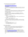
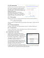
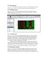
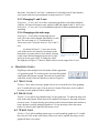
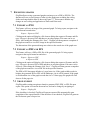
iTagPlot User Manual
iTagPlot is a tool to accurately compute and interactively visualize tag density (read coverage)
from genomic sequencing data. The software includes a computing module, highly interactive
user interface and graphing tools with many options for creating tag density and customizing the
graph. iTagPlot computes and draws the average tag density of all or groups of features for each
sample. In addition, iTagPlot computes and visualizes the tag density of individual features of
interest, and groups of features based on quantitative values such as gene expression, DNA
methylation, CpG density, and even quantiles of quantitative values. The software supports
parallel computation using a grid engine and customize drawing properties easily in a userfriendly interface. Given that tag density plots are a mainstay of manuscripts describing
epigenomics data-based on next-gen sequencing, it is essential for biologists to have access to
software that can generate these plots easily.
Table of Contents
1! Getting started ........................................................................................................................... 3!
1.1! Prerequisites ....................................................................................................................... 3!
1.2! installing and using iTagPlot ............................................................................................. 4!
1.2.1! Mac OS X ................................................................................................................... 4!
1.2.2! MS Windows .............................................................................................................. 4!
1.2.3! Linux or UNIX............................................................................................................ 4!
2! Data File Format ....................................................................................................................... 4!
2.1! Sequence Mapping file ...................................................................................................... 4!
2.2! Annotation File .................................................................................................................. 5!
2.3! Annotation configuration file............................................................................................. 5!
2.4! Tag Density file.................................................................................................................. 6!
2.5! Group file ........................................................................................................................... 6!
2.6! Quantity file ....................................................................................................................... 6!
3! Computation of tag density ....................................................................................................... 7!
3.1! Enrichment data ................................................................................................................. 7!
3.2! Score data ........................................................................................................................... 8!
4! Loading data.............................................................................................................................. 8!
4.1! Sample................................................................................................................................ 8!
4.1.1! Open sample................................................................................................................ 8!
4.1.2! Delete sample .............................................................................................................. 9!
4.1.3! Change sample name .................................................................................................. 9!
4.1.4! Context menu .............................................................................................................. 9!
4.2! Group ................................................................................................................................. 9!
4.2.1! Open group.................................................................................................................. 9!
4.2.2! Quantity group ............................................................................................................ 9!
4.2.3! K-Means.................................................................................................................... 10!
4.2.4! ID conversion ............................................................................................................ 11!
4.2.5! Delete group .............................................................................................................. 11!
4.2.6! Change group name .................................................................................................. 11!
4.2.7! Context menu ............................................................................................................ 11!
4.3! Searching feature ............................................................................................................. 11!
5! Visualization ........................................................................................................................... 12!
5.1! Generating a plot .............................................................................................................. 12!
5.2! Manipulating visualiztion ................................................................................................ 13!
5.2.1! Editing graph............................................................................................................. 14!
5.2.2! Editing heatmap ........................................................................................................ 14!
5.2.3! Changing colors ........................................................................................................ 14!
5.2.4! Editing text and fonts ................................................................................................ 14!
5.2.5! Changing X- and Y-axis ........................................................................................... 15!
5.2.6! Changing scale and range ......................................................................................... 15!
6! Graphing tools......................................................................................................................... 15!
6.1! Move tool ......................................................................................................................... 15!
6.2! Draw tool ......................................................................................................................... 15!
6.3! Write tool ......................................................................................................................... 15!
7! Exporting graphs ..................................................................................................................... 16!
7.1! Export as PNG ................................................................................................................. 16!
7.2! Export as PDF and EPS ................................................................................................... 16!
7.3! Show export ..................................................................................................................... 16!
8! Other functionality .................................................................................................................. 17!
8.1! Saving preferences ........................................................................................................... 17!
8.2! Sidepanels visibility ......................................................................................................... 17!
8.2.1! Show sidepanels ........................................................................................................ 17!
8.2.2! Hide sidepanels ......................................................................................................... 17!
8.2.3! Hide data panel only ................................................................................................. 17!
8.3! Errors................................................................................................................................ 17!
1 GETTING STARTED
1.1 PREREQUISITES
To use iTagPlot, you will need the following programs:
• perl 5.8.5 or later
• samtools 0.1.6 or later
• perl modules in most perl distribution as default
Getopt::Long, File::Basename, File::Which, File::Spec, Cwd, POSIX
You need to add the directory of perl and samtools into your PATH.
1.2 INSTALLING AND USING ITAGPLOT
You can download the release and data from
https://sourceforge.net/projects/itagplot/files/release/.
!"#"! $%&'()'*'
For installation, download iTagPlot-0.9-macosx.dmg, double click the file, and drag and
drop the icon into the Application folder. To run it, double click the desktop icon or start
menu.
!"#"# $)'+,-./01'
For installation, download iTagPlot-0.9-windows7.msi and iTagPlot-0.9-windows8.msi
and double click the file. To run it, double click the desktop icon or start menu.
!"#"2 3,-45'/6'789*'
For installation, download an appropriate version of iTagPlot-0.9-*.x86_64.deb,
iTagPlot-0.9-*.x86_64.rpm, and iTagPlot-0.9-JDK-1.7.0_51.zip and run a following
command as root or non-root.
For a RPM file:
as root:
rpm -ivh iTagPlot-0.9-*.rpm
as non-root: rpm --install --badreloc --relocate /=$HOME --dbpath $HOME/rpm_db
--nodeps --noscripts iTagPlot-0.9-*.rpm
For a DEB file:
as root:
dpkg -i iTagPlot-0.9-*.deb
as non-root: dpkg-deb -x iTagPlot-0.9-*.deb $HOME
The command for root and non-root installs to /opt/iTagPlot and $HOME/opt/iTagPlot,
respectively. To run it, double click the desktop icon or start menu, or use the command
line.
For a ZIP file:
unzip iTagPlot-0.9-JDK-1.7.0_51.zip -d out_dir
To run it, run the following command
out_dir/iTagPlot-0.9-JDK-1.7.0_51/iTagPlot.sh
2 DATA FILE FORMAT
iTagPlot accepts data as a BAM or BED file for mapped reads and BED files for
annotation to compute tag density of a sample. The computation module generates a file
for tag density. The visualization module accepts a group file or quantity file.
2.1 SEQUENCE MAPPING FILE
Most mapping programs can generate a BAM file after mapping reads to reference
sequences (http://samtools.sourceforge.net/SAM1.pdf). A BED file is a tab-delimitated
file and can store two different types of data. In Table 2.1, the first row represents a
mapped read and the second represents the score of a region. While iTagPlot counts the
number of mapped reads for the former, it uses the 5th column to average the score for the
latter.
Table 2.1: Example of BED formats.
chr1
1167000
1168985
read1
…
chr11
127494
127496
cg13501959
0.596681809
2.2 ANNOTATION FILE
An annotation file can be downloaded from online database servers, e.g., the UCSC
genome browser, into various BED format because genomic features have different
attributes. In Table 2.2, the rows represent the annotation of RefSeq genes, CpG islands,
and DNase clusters. They have different number of columns.
Table 2.2: Example of annotation.
chr21
11020841
11098925
BAGE3
chr21
10895511
10895781
CpG: 30
chr21
15355105
15355308
FAIREOnly_70565
NM_182481
-
1000
.
15355105
15355308
2.3 ANNOTATION CONFIGURATION FILE
For easy computation of tag density, iTagPlot uses an annotation configuration file
(Table 2.3). The first and second columns represent the name and file of each feature,
respectively. The third represents column numbers that are used to build an identifier of
features in a tag density file. The fourth and fifth represent the number of bins in body
and up/down-stream of features. The sixth represents the length of up/down-stream. The
last specifies in which regions tag density is computed: 5 for up-stream and body, 3 for
body and down-stream, and 0 for all regions. As shown in the last row, reference
sequences to be filtered can be specified.
Table 2.3: Example of annotation configuration file.
#Name
File
IDCol
BodyBin
StreamBin
StreamLength
Type
cgi
hg19.cpgisland.bed
4
200
200
4000
0
dnase
hg19.dnase.bed
4
200
100
500
0
refseq
hg19.refseq.bed
4,5
500
500
5000
0
tss
hg19.refseq.bed
4,5
500
500
5000
5
tts
hg19.refseq.bed
4,5
500
500
5000
3
filter
chrM
2.4 TAG DENSITY FILE
Tag density file uses newline character as a row separator and tab as a column separator.
There has to be the same number of columns for each row. The number of rows is not
limited. The first row describes the data headers and will be used to populate the graph
axes. All subsequent rows describe features and contain the plot data.
Table 2.4 displays a simplified example of sample file structure. iTagPlot data parser will
interpret sample columns as follows:
1. Feature name
2. Feature chromosome (type string)
3. Start value (type int)
4. End value (type int)
5. Strand (ignored)
6…n
Feature data (type double)
Table 2.4: Example of tag density file.
#Key
Ref
Start
End
Strand
-5000
-4980
-4960
-4940
CpG2400
chr1
1167000
1168985
.
1.844
1.800
1.862
1.895
CpG2753
chr1
1173914
1174263
.
1.929
2.072
2.156
2.211
2.5 GROUP FILE
Group file includes list of feature names separated by tab character. Table 2.5 shows an
example of group file structure. The purpose of the group file is to allow easy creation of
subsets of features and calculating the average of the subset data. Therefore user should
upload sample files before group files.
iTagPlot parser will read the contents of the group file and look for matches in the names
of existing features. iTagPlot will ignore group file if it does not match any existing
features.
Table 2.5: Example of group file.
21:NM_152486:SAMD11 22:NM_015658:NOC2L
23:NM_198317:KLHL17
28:NM_001142467:HES4
30:NM_198576:AGRN
32:NM_017891:C1orf159
39:NM_004195:TNFRSF18
41:NM_148902:TNFRSF18 45:NM_080605:B3GALT6 43:NM_016176:SDF4
44:NM_016547:SDF4
46:NM_001014980:FAM132A
2.6 QUANTITY FILE
Quantity file includes list of feature names along with quantitative values such as
expression and methylation for samples. Table 2.6 shows an example of quantity file
structure. The purpose of the quantity file is to allow easy creation of subsets (groups) of
features based on quantitative values and calculating the average of the subset data.
Therefore user should upload sample files before quantity files.
Table 2.6: Example of quantity file.
Gene
DNMT1
DNMT3B
NTC
AAAS
8.81842
7.73616
7.96755
ABCA5
10.3893
9.589765
9.413465
3 COMPUTATION OF TAG DENSITY
To compute tag density of enrichment data (mapped reads), users specify input files in
the BAM or BED format, an annotation configuration file, an output directory, and
choose Enrichment for Data Type. An annotation base directory should be specified if a
configuration file is in the different directory of annotation files. iTagPlot supports
several running modes to use a single and multiple cores and grid engine. Users should
specify the command for a grid engine.
3.1 ENRICHMENT DATA
Figure 3.1 shows an example to compute tag density for 6 ChIP-seq datasets using a grid
engine with 4 jobs. Note that the input files have mapped reads and the fragment size
should be specified to lengthen reads to the original size.
Figure 3.1: Tag density computation for 7 sequencing datasets in the BAM format using a grid engine with 4
jobs.
3.2 SCORE DATA
Figure 3.2 shows an example to compute tag density for score-based data. The column
number should be specified for the score.
Figure 3.2: Tag density computation of Infinium 450K array data in the BED format with 4 cores.
4 LOADING DATA
4.1 SAMPLE
:"!"! (;<-'1%=;><'
To load samples, navigate to the top menu bar and select:
Sample > Open Sample (Figure 4.1)
iTagPlot will attempt to retrieve and parse the requested file. A
blue progress bar will appear in the interface to indicate load
Figure 4.1: Sample menu.
process is being handled. After samples are successfully
read, the samples and their features will appear in the user
interface as shown in Figure 4.2.
4.1.2 Delete sample
To delete samples, choose or check samples and navigate
to the top menu bar and select:
Sample > Delete Checked Sample
or Delete Selected Sample
4.1.3 Change sample name
To change a sample name, click the sample name in
Figure 4.2, and then edit the name.
4.1.4 Context menu
To show a context menu, click the right button of mouse.
It has several functions to check/uncheck and
select/unselect samples.
Figure 4.2: Sample and feature
tables.
4.2 GROUP
iTagPlot supports various way to define a group of features. (1)
a group file list features that belong to the group, (2) a quantity
file has quantitative values such as gene expression, DNA
methylation, and enrichment scores, that use to define groups
based on criteria, (3) k-means clustering algorithm is applied to
determine groups based on tag density, and (4) MSigDB is a
database to define gene sets related to biological function and
pathway.
:"#"! (;<-'?6/4;'
To load a group, navigate to the top menu bar and select:
Figure 4.3: Group menu.
Group > Open Group (Figure 4.3)
iTagPlot will show a dialog for ID conversion, attempt to
retrieve and parse the requested file. A blue progress bar
will appear in the interface to indicate load process is
being handled. After a group is successfully read, the
group will appear in the user interface as shown in Figure
4.4.
Figure 4.4: Goup table.
:"#"# @4%-A,AB'?6/4;'
To load groups based on quantitative values, navigate to the top menu bar and select:
Group > Quantity Group > Microarray, RNA-seq, Beta Values, or Quantile
iTagPlot will show dialogs for ID conversion, attempt to retrieve and parse the requested
file. A blue progress bar will appear in the interface to indicate load process is
Figure 4.5: Quantity group dialog. Users can change criteria for grouping and choose sample names.
:"#"2 CD$<%-1'
To group (cluster) features based on tag density,
navigate to the top menu bar and select:
Group > K-Means (Figure 4.3)
iTagPlot will show a dialog for options (Figure 4.6),
apply the k-means algorithm to cluster features and
samples based on tag density.
The result of clustering can be saved and opened with
menu Save and Open (figure).
Figure 4.6: Cluster option dialog.
:"#": 9E'&/-F<61,/-'
iTagPlot has a great function to map IDs in group
files to those in sample files because annotation
for groups could use different ID convention. As
shown in Figure 4.7, users specify a delimiter and
starting and end indices.
GSTP1|NM_000852|1461 is converted to
NM_000582 with delimiter of ‘|’, and starting
and end indices of 1 and 1. If IDs in samples and
groups are the same, users click button “cancer”.
4.2.5 Delete group
Figure 4.7: ID convention dialog.
To delete groups, choose or check groups and navigate to the top menu bar and select:
Sample > Delete Checked Group
or Delete Selected Group
The user interface will update and the selected groups will no longer be visible in the lists
of groups.
4.2.6 Change group name
To change a group name, click the group name in Figure 4.2, and then edit the name.
4.2.7 Context menu
To show a context menu, click the right button of mouse. It has several functions to
check/uncheck and select/unselect groups.
4.3 SEARCHING FEATURE
iTagPlot enables searching through uploaded
features using a search function. To use this feature,
navigate to the left of the interface, and look for a
bar with label “Search features”. Clicking on the bar
will toggle the visibility of the search field. The
search field is displayed in Figure 4.8.
To search for specific features, type a text into the
search field and press ENTER. iTagPlot will search
for matches in feature whose name contains the
substring entered into the search field.
Figure 4.8: Search feature.
To clear the search results and redisplay the full list
of features, either delete the input from the search field and press ENTER, or click on the
“Search features” bar. The latter will also hide the search field.
5 VISUALIZATION
5.1 GENERATING A PLOT
Generating a plot requires some data is first loaded into
the system. iTagPlot allows plotting a selection of
samples, features, and groups.
To generate a plot navigate to the left of user interface and
select samples and features and/or groups you wish to
visualize. Select one or more items from by clicking on
the checkbox next to its name. Figure 5.1 illustrates
selecting two features. To deselect a data item click on the
checkbox again until the checkmark disappears.
After selecting one or more items, click on the “Chart” or
“Heatmap” button in the top left corner. A chart or
heatmap will appear in the view panel as shown in Figure
5.2 or Figure 5.3.
Figure 5.2: Generated graph.
Figure 5.1: Selecting data items.
Figure 5.3: Generated heatmap.
Note that chosen features and groups will be enumerated for each chosen sample and the
checkbox “I” will not draw the date items as shown in Figure 5.4.
Figure 5.4: Area graph for various groups without drawing features.
5.2 MANIPULATING VISUALIZTION
iTagPlot allows customizing many aspects of the visualization using the toolbar as shown
in Figure 5.5.
Figure 5.5: Preference toolbar.
G"#"! H.,A,-?'?6%;I'
Preferences > Graph allows customizing several aspects of the graph: graph type, legend
location, and point mark, line weight, and maximum number of seriesEditing colors.
G"#"# H.,A,-?'I<%A=%;'
Preferences > Cluster allows customizing several aspects of the heatmap: clustering
algorithm, samples in a row, distance metric, linkage method, the number of clusters for
k-means, and the height of rows in pixel.
Figure 5.6: Heatmap with samples in a row.
5.2.3 Changing colors
Preferences > Colors allows customizing graph and heatmap colors. Users can change
the following options: drawing area (graph background), graph area (plot background),
graph border, graph title color, axes labels color, legend labels, legend background, xaxis gridlines, y-axis gridlines, tick labels (along axes), tick lines (along axes), symbol
fill. These values can be set to any color in the RGB range. For heatmap, users can
choose preset color scheme or change colors for gradient.
iTagPlot also allows changing data series colors. To change a plot color, hover
over the specific series line or area, which will change the mouse cursor to a hand. Then
right click on the mouse and a context menu will appear. For line graph there is an option
to change the line color. For an area graph there is an option to change the line color and
area fill color. Changing the current selection will change the series color respectively.
G"#": H.,A,-?'A<5A'%-.'J/-A1'
Preferences > Labels allows setting and changing graph title and axes labels. These are
all optional and can also be left blank. It also allows customizing axes fonts. The axes
fonts are controlled by the same variable and therefore cannot be set to different values
for each axis. If or once the object is set to Axes, you will see the current settings for axes
font in the “Font family” and “Size” comboboxes. Font family lists all fonts found in
your system, and sizes a preconfigured to range between 6-57 pixels.
G"#"G KI%-?,-?'*D'%-.'LD%5,1'
Preferences > X-Axis and Y-Axis allow customizing grid lines, tick marks and labels
visibility, tick interval and max count, and tick width and length for the X- and Y-axis.
Preferences > X-Axis and Y-Axis has additional options for data transformation and
smoothing.
G"#"M KI%-?,-?'1&%><'%-.'6%-?<'
Preferences > Scale allows customizing the axis
scale. The scale can be changed individually for each
axis. The scale range is 1-2.5 and defaults to 1.
“Reset axis scales” resets the scale to 1 for X- and Yaxis.
As shown in Figure 5.7, users can use axis
scale sliders in the view panel by hovering over the
5.7: Axis scale sliders
horizontal x-axis and vertical y-axis sliders, clicking Figure
(left) and Y-axis range slider
on the control ball and dragging mouse left or right
(right).
and up or down, respectively, to change the value.
The right plot of Figure 5.7 shows a double slider to set the range of the Y-axis.
6 GRAPHING TOOLS
iTagPlot provides multiple tools for further edit the appearance
of a generated graph. To use these tools, user must first upload
sample data and generate a graph. The tools are located in the
control bar on top of the user interface as show in Figure 6.1.
Figure 6.1: Toolbox toolbar.
6.1 MOVE TOOL
Toolbox > Move allows moving a graph once its size exceeds the size of the graphing
area. To enable the move tool, click on the move button. When move tool is enabled,
hovering over the graph will show a hand cursor.
6.2 DRAW TOOL
Toolbox > Draw allows free-hand drawing over the graph area. To enable the draw tool,
click on the draw button. When draw tool is enabled, hovering over the graph will show
an arrow cursor. To begin drawing, press down on the left mouse button and continue to
keep it down as you drag along the graph area. To stop drawing, release the mouse
button. To delete a path, right-click the mouse over it.
6.3 WRITE TOOL
Toolbox > Write allows adding custom texts over and around the graph area. To enable
the write tool, click on the write button. When write tool is enabled, hovering over the
graph will show a text cursor.
7 EXPORTING GRAPHS
iTagPlot allows saving a generated graph as an image or as a PDF or EPS file. The
function will save an exact image of what is in the graph area excluding the scaling
sliders and range double slider as shown in Figure 5.7. This means it includes any
changes to axes scaling and application of Draw and Write tools.
7.1 EXPORT AS PNG
This feature will save an image of the generated graph. To being export, navigate to the
top left menu bar and select:
Export > Export as PNG
Clicking on the option will display a file chooser dialog that request a file name and file
type. File type is preset to PNG and there are no other options. File name can be set
freely. After setting the filename click “Save”. iTagPlot will then generate a snapshot of
the graph area and save it as PNG image in the specified location.
The dimensions of the generated image are relative to the actual size of the graph area.
7.2 EXPORT AS PDF AND EPS
This feature will save a PDF or EPS file of the generated graph. To being export,
navigate to the top left menu bar and select:
Export > Export as PDF
or Export as EPS
Clicking on the option will display a file chooser dialog that request a file name and file
type. File type is preset to PDF or EPS and there are no other options. File name can be
set freely. After setting the filename click “Save”. iTagPlot will then generate a snapshot
of the graph area and save it as a PDF file in the specified location.
The PDF or EPS document defaults to 1-page letter size. If the graph width exceeds its
heights, the generated PDF or EPS will be landscape, else it will be portrait. If the graph
is scaled and the size of the graph exceeds the size of 1 letter page, the graph will scale
down to fit the page size.
7.3 SHOW EXPORT
iTagPlot enables setting an option to launch a generated PNG, PDF, or EPS file upon
export. This option is located in the menu bar, and can be change by navigating to:
Export > Display file
If the checkbox is checked, iTagPlot will open an exported file automatically upon
completion of the export function. If the checkbox is not checked, iTagPlot will generate
the file but not open it for preview.
8 OTHER FUNCTIONALITY
8.1 SAVING PREFERENCES
iTagPlot will automatically save preferences such as graph type, colors, fonts etc. This
functionality is enabled by default and will execute whenever preferences are changed.
The settings will be saved in the same file where the executable application is saved, so it
is advisable to save the application in a writable directory. The preferences are saved in a
file titled “settings”. If this file is deleted or corrupted, graph preferences are set to their
defaults.
8.2 SIDEPANELS VISIBILITY
To enhance analyzing the graph, it is possible to toggle the visibility of both data panels
on the left and control bar on top of the user interface.
8.2.1 Show sidepanels
To hide both panels, press CTRL+1, or use the top menu bar and navigate to:
View > Collapse Sidepanels
8.2.2 Hide sidepanels
To show both panels, press CTRL+2, or use the top menu bar and navigate to:
View > Show Sidepanels
8.2.3 Hide data panel only
To adjust the size and/or visibility of data panels only, bovver over the vertical
separator between the data panels and the graph area, click and drag the mouse.
Dragging to the left will reduce the width or hide the panel, and dragging to the right
will increase its width.
8.3 ERRORS
iTagPlot will generate error messages when invalid
requests occur. The error message appears in the top
right corner of the user interface. The error message
includes a header and short description of the cause.
Error messages fade automatically after a few
seconds, or it can be hidden immediately by clicking
on a “X” icon in the top right corner. Figure 8.1
shows a sample error message.
Figure 8.1: Error message box.