Download the manual for gprMax

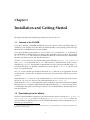
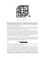
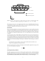
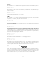
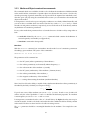
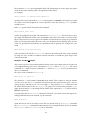
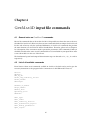
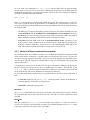
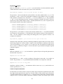
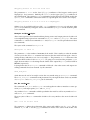
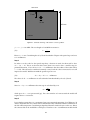
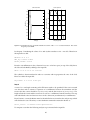
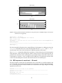
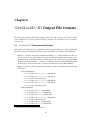
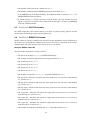
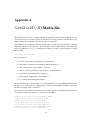
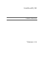
"ricker" Waveform
Power spectrum
1
0
0.8
−10
0.6
Normalised Power [db]
0.4
Amplitude
0.2
0
−0.2
−20
−30
−40
−0.4
−0.6
−50
−0.8
−1
0
2
4
Time [ns]
6
−60
0
8
1000
2000
3000
Frequency [MHz]
4000
Figure 5.2: Normalized power spectrum and time waveform of the ricker excitation function. The centre
frequency is 900 MHz.
be adequate. Considering the values of ∆x and ∆y this translates to 240 × 120 cells. Therefore in
the input file we add:
#domain: 0.6 0.3
#dx_dy: 0.0025 0.0025
#time_window: 8.0e-9
From the 300 millimetres in the y direction let us use 50 for free space (on top of the slab) hence
the slab can be defined by adding to the input file:
#box: 0.0 0.0 0.6 0.25 concrete
The cylinder is then introduced in order to overwrite with its properties the ones of the slab.
Hence we add to the input file:
#cylinder: 0.3 0.175 0.025 pec
Step 6
A scan of 42.5 cm length consisting of 41 GPR traces needs to be specified. If the scan is centred
over the rebar and we assume a separation of 50 millimetres between the transmitter and the
receiver the first source should be at (0.075,0.2525) and the first receiver at (0.125,0.2525). The
height of both the source and the receiver is set to be at 2.5 millimetres from the interface. The step
with which both source and receiver moves in the x direction (scan direction) is 10 millimetres.
From Version 2 a source definition must be inlcuded before we introduce the analysis step which
will calculate the scan. Therefore, a source defintion command is inserted in the file as:
#line_source: 1.0 900e6 ricker MyLineSource
To compute a scan then the following analysis step is inserted in the input file
45