Download pdf format

i
E CL P S
e
An Introduction
Andrew M. Cheadle
Warwick Harvey
Andrew J. Sadler
Kish Shen
Mark G. Wallace
ECLi PSe Group
IC-Parc
Imperial College London
November 21, 2002
Joachim Schimpf
c Imperial College London 2002
°
Contents
1 Introduction
1
2 Getting started with ECLi PSe
2.1 How do I install the ECLi PSe system? . . . . . .
2.2 How do I read the online documentation? . . . .
2.3 How do I run my ECLi PSe programs? . . . . . .
2.4 How do I use tkeclipse? . . . . . . . . . . . . .
2.4.1 Getting started . . . . . . . . . . . . . . .
2.4.2 Compiling a program . . . . . . . . . . .
2.4.3 Executing a query . . . . . . . . . . . . .
2.4.4 Editing a file . . . . . . . . . . . . . . . .
2.4.5 Debugging a program . . . . . . . . . . .
2.4.6 Getting help . . . . . . . . . . . . . . . .
2.4.7 Other tools . . . . . . . . . . . . . . . . .
2.5 How do I make things happen at compile time? .
2.6 How do I use ECLi PSe libraries in my programs?
2.7 Other tips . . . . . . . . . . . . . . . . . . . . . .
2.7.1 Recommended file names . . . . . . . . .
3 Prolog Introduction
3.1 Terms and their data types . . . . .
3.1.1 Numbers . . . . . . . . . . .
3.1.2 Strings . . . . . . . . . . . . .
3.1.3 Atoms . . . . . . . . . . . . .
3.1.4 Lists . . . . . . . . . . . . . .
3.1.5 Structures . . . . . . . . . . .
3.2 Predicates, Goals and Queries . . . .
3.2.1 Conjunction and Disjunction
3.3 Unification and Logical Variables . .
3.3.1 Symbolic Equality . . . . . .
3.3.2 Logical Variables . . . . . . .
3.3.3 Unification . . . . . . . . . .
3.4 Defining Your Own Predicates . . .
3.4.1 Comments . . . . . . . . . . .
.
.
.
.
.
.
.
.
.
.
.
.
.
.
i
.
.
.
.
.
.
.
.
.
.
.
.
.
.
.
.
.
.
.
.
.
.
.
.
.
.
.
.
.
.
.
.
.
.
.
.
.
.
.
.
.
.
.
.
.
.
.
.
.
.
.
.
.
.
.
.
.
.
.
.
.
.
.
.
.
.
.
.
.
.
.
.
.
.
.
.
.
.
.
.
.
.
.
.
.
.
.
.
.
.
.
.
.
.
.
.
.
.
.
.
.
.
.
.
.
.
.
.
.
.
.
.
.
.
.
.
.
.
.
.
.
.
.
.
.
.
.
.
.
.
.
.
.
.
.
.
.
.
.
.
.
.
.
.
.
.
.
.
.
.
.
.
.
.
.
.
.
.
.
.
.
.
.
.
.
.
.
.
.
.
.
.
.
.
.
.
.
.
.
.
.
.
.
.
.
.
.
.
.
.
.
.
.
.
.
.
.
.
.
.
.
.
.
.
.
.
.
.
.
.
.
.
.
.
.
.
.
.
.
.
.
.
.
.
.
.
.
.
.
.
.
.
.
.
.
.
.
.
.
.
.
.
.
.
.
.
.
.
.
.
.
.
.
.
.
.
.
.
.
.
.
.
.
.
.
.
.
.
.
.
.
.
.
.
.
.
.
.
.
.
.
.
.
.
.
.
.
.
.
.
.
.
.
.
.
.
.
.
.
.
.
.
.
.
.
.
.
.
.
.
.
.
.
.
.
.
.
.
.
.
.
.
.
.
.
.
.
.
.
.
.
.
.
.
.
.
.
.
.
.
.
.
.
.
.
.
.
.
.
.
.
.
.
.
.
.
.
.
.
.
.
.
.
.
.
.
.
.
.
.
.
.
.
.
.
.
.
.
.
.
.
.
.
.
.
.
.
.
.
.
.
.
.
.
.
.
.
.
.
.
.
.
.
.
.
.
.
.
.
.
.
.
.
.
.
.
.
.
.
.
.
.
.
.
.
.
.
.
.
.
.
.
.
.
.
.
.
.
.
.
.
.
.
.
.
.
.
.
.
.
.
.
.
.
.
.
.
.
.
.
.
.
.
.
.
.
.
.
.
.
.
.
.
.
.
.
.
.
.
.
.
.
.
.
.
.
.
.
.
.
.
.
.
.
.
.
.
.
.
.
.
.
.
.
.
.
.
.
.
.
.
.
.
.
.
.
.
.
.
.
.
.
.
.
.
.
.
.
.
.
.
.
.
.
.
.
.
.
.
.
.
.
.
.
.
.
.
.
.
.
.
.
.
.
.
.
.
.
.
.
.
.
.
.
.
.
.
.
.
.
.
.
.
.
.
.
.
.
.
.
.
.
.
.
.
.
.
.
.
.
.
.
3
3
3
3
3
3
4
4
5
5
5
6
7
8
8
8
.
.
.
.
.
.
.
.
.
.
.
.
.
.
9
9
9
10
10
10
11
12
13
13
13
14
14
15
15
3.4.2 Clauses and Predicates . . . .
3.5 Execution Scheme . . . . . . . . . .
3.5.1 Resolution . . . . . . . . . . .
3.6 Partial data structures . . . . . . . .
3.7 More control structures . . . . . . .
3.7.1 Disjunction . . . . . . . . . .
3.7.2 Conditional . . . . . . . . . .
3.7.3 Call . . . . . . . . . . . . . .
3.7.4 All Solutions . . . . . . . . .
3.8 Using Cut . . . . . . . . . . . . . . .
3.8.1 Commit to current clause . .
3.8.2 Prune alternative solutions .
3.9 Common Pitfalls . . . . . . . . . . .
3.9.1 Unification works both ways .
3.9.2 Unexpected backtracking . .
3.10 Exercises . . . . . . . . . . . . . . .
.
.
.
.
.
.
.
.
.
.
.
.
.
.
.
.
.
.
.
.
.
.
.
.
.
.
.
.
.
.
.
.
.
.
.
.
.
.
.
.
.
.
.
.
.
.
.
.
.
.
.
.
.
.
.
.
.
.
.
.
.
.
.
.
.
.
.
.
.
.
.
.
.
.
.
.
.
.
.
.
4 ECLi PSe Programming
4.1 Structure Notation . . . . . . . . . . . . . . .
4.2 Loops . . . . . . . . . . . . . . . . . . . . . .
4.3 Working with Arrays of Items . . . . . . . . .
4.4 Storing Information Across Backtracking . . .
4.4.1 Bags . . . . . . . . . . . . . . . . . . .
4.4.2 Shelves . . . . . . . . . . . . . . . . .
4.5 Input and Output . . . . . . . . . . . . . . .
4.5.1 Printing ECLi PSe Terms . . . . . . .
4.5.2 Reading ECLi PSe Terms . . . . . . .
4.5.3 Formatted Output . . . . . . . . . . .
4.5.4 Streams . . . . . . . . . . . . . . . . .
4.6 Matching . . . . . . . . . . . . . . . . . . . .
4.7 List processing . . . . . . . . . . . . . . . . .
4.8 String processing . . . . . . . . . . . . . . . .
4.9 Term processing . . . . . . . . . . . . . . . .
4.10 Module System . . . . . . . . . . . . . . . . .
4.10.1 Overview . . . . . . . . . . . . . . . .
4.10.2 Making a Module . . . . . . . . . . . .
4.10.3 Using a Module . . . . . . . . . . . . .
4.10.4 Qualified Goals . . . . . . . . . . . . .
4.10.5 Exporting items other than Predicates
4.11 Exception Handling . . . . . . . . . . . . . .
4.12 Time and Memory . . . . . . . . . . . . . . .
4.12.1 Timing . . . . . . . . . . . . . . . . .
4.13 Exercises . . . . . . . . . . . . . . . . . . . .
ii
.
.
.
.
.
.
.
.
.
.
.
.
.
.
.
.
.
.
.
.
.
.
.
.
.
.
.
.
.
.
.
.
.
.
.
.
.
.
.
.
.
.
.
.
.
.
.
.
.
.
.
.
.
.
.
.
.
.
.
.
.
.
.
.
.
.
.
.
.
.
.
.
.
.
.
.
.
.
.
.
.
.
.
.
.
.
.
.
.
.
.
.
.
.
.
.
.
.
.
.
.
.
.
.
.
.
.
.
.
.
.
.
.
.
.
.
.
.
.
.
.
.
.
.
.
.
.
.
.
.
.
.
.
.
.
.
.
.
.
.
.
.
.
.
.
.
.
.
.
.
.
.
.
.
.
.
.
.
.
.
.
.
.
.
.
.
.
.
.
.
.
.
.
.
.
.
.
.
.
.
.
.
.
.
.
.
.
.
.
.
.
.
.
.
.
.
.
.
.
.
.
.
.
.
.
.
.
.
.
.
.
.
.
.
.
.
.
.
.
.
.
.
.
.
.
.
.
.
.
.
.
.
.
.
.
.
.
.
.
.
.
.
.
.
.
.
.
.
.
.
.
.
.
.
.
.
.
.
.
.
.
.
.
.
.
.
.
.
.
.
.
.
.
.
.
.
.
.
.
.
.
.
.
.
.
.
.
.
.
.
.
.
.
.
.
.
.
.
.
.
.
.
.
.
.
.
.
.
.
.
.
.
.
.
.
.
.
.
.
.
.
.
.
.
.
.
.
.
.
.
.
.
.
.
.
.
.
.
.
.
.
.
.
.
.
.
.
.
.
.
.
.
.
.
.
.
.
.
.
.
.
.
.
.
.
.
.
.
.
.
.
.
.
.
.
.
.
.
.
.
.
.
.
.
.
.
.
.
.
.
.
.
.
.
.
.
.
.
.
.
.
.
.
.
.
.
.
.
.
.
.
.
.
.
.
.
.
.
.
.
.
.
.
.
.
.
.
.
.
.
.
.
.
.
.
.
.
.
.
.
.
.
.
.
.
.
.
.
.
.
.
.
.
.
.
.
.
.
.
.
.
.
.
.
.
.
.
.
.
.
.
.
.
.
.
.
.
.
.
.
.
.
.
.
.
.
.
.
.
.
.
.
.
.
.
.
.
.
.
.
.
.
.
.
.
.
.
.
.
.
.
.
.
.
.
.
.
.
.
.
.
.
.
.
.
.
.
.
.
.
.
.
.
.
.
.
.
.
.
.
.
.
.
.
.
.
.
.
.
.
.
.
.
.
.
.
.
.
.
.
.
.
.
.
.
.
.
.
.
.
.
.
.
.
.
.
.
.
.
.
.
.
.
.
.
.
.
.
.
.
.
.
.
.
.
.
.
.
.
.
.
.
.
.
.
.
.
.
.
.
.
.
.
.
.
.
.
.
.
.
.
.
.
.
.
.
.
.
.
.
.
.
.
.
.
.
.
.
.
.
.
.
.
.
.
.
.
.
.
.
.
.
.
.
.
.
.
.
.
.
.
.
.
.
.
.
.
.
.
.
.
.
.
.
.
.
.
.
.
.
.
.
.
.
.
.
.
.
.
.
.
.
.
.
.
.
.
.
.
.
.
.
.
.
.
.
.
.
.
.
.
.
.
.
.
.
.
.
.
.
.
.
.
.
.
.
.
.
.
.
.
.
.
.
.
.
.
.
.
.
.
.
.
.
.
.
.
.
.
.
.
.
.
.
.
.
.
.
.
.
.
.
.
.
.
.
.
.
.
.
.
.
.
.
.
.
.
.
.
.
.
.
.
.
.
.
.
.
.
.
.
.
.
.
.
15
17
17
19
20
20
20
21
21
21
22
22
22
23
23
24
.
.
.
.
.
.
.
.
.
.
.
.
.
.
.
.
.
.
.
.
.
.
.
.
.
25
25
26
27
28
28
29
29
29
30
31
32
32
34
35
35
36
36
36
36
37
38
38
39
39
40
5 A Tutorial Tour of Debugging in TkECLi PSe
5.1 The Buggy Program . . . . . . . . . . . . . . .
5.2 Running the Program . . . . . . . . . . . . . .
5.3 Debugging the Program . . . . . . . . . . . . .
5.4 Summary . . . . . . . . . . . . . . . . . . . . .
5.4.1 TkECLi PSe toplevel . . . . . . . . . . .
5.4.2 Predicate Browser . . . . . . . . . . . .
5.4.3 Tracer . . . . . . . . . . . . . . . . . . .
5.4.4 Tracer Filter . . . . . . . . . . . . . . .
5.4.5 Term Inspector . . . . . . . . . . . . . .
5.4.6 Delayed Goals Viewer . . . . . . . . . .
.
.
.
.
.
.
.
.
.
.
.
.
.
.
.
.
.
.
.
.
.
.
.
.
.
.
.
.
.
.
.
.
.
.
.
.
.
.
.
.
.
.
.
.
.
.
.
.
.
.
.
.
.
.
.
.
.
.
.
.
.
.
.
.
.
.
.
.
.
.
.
.
.
.
.
.
.
.
.
.
.
.
.
.
.
.
.
.
.
.
.
.
.
.
.
.
.
.
.
.
.
.
.
.
.
.
.
.
.
.
.
.
.
.
.
.
.
.
.
.
.
.
.
.
.
.
.
.
.
.
.
.
.
.
.
.
.
.
.
.
.
.
.
.
.
.
.
.
.
.
.
.
.
.
.
.
.
.
.
.
.
.
.
.
.
.
.
.
.
.
.
.
.
.
.
.
.
.
.
.
.
.
.
.
.
.
.
.
.
.
41
42
43
43
50
50
51
52
52
53
53
6 Program Analysis
6.1 What tools are available?
6.2 Profiler . . . . . . . . . .
6.3 Line coverage . . . . . . .
6.3.1 Compilation . . . .
6.3.2 Results . . . . . .
.
.
.
.
.
.
.
.
.
.
.
.
.
.
.
.
.
.
.
.
.
.
.
.
.
.
.
.
.
.
.
.
.
.
.
.
.
.
.
.
.
.
.
.
.
.
.
.
.
.
.
.
.
.
.
.
.
.
.
.
.
.
.
.
.
.
.
.
.
.
.
.
.
.
.
.
.
.
.
.
.
.
.
.
.
.
.
.
.
.
.
.
.
.
.
55
55
55
58
59
60
.
.
.
.
.
.
.
.
.
.
.
.
.
.
.
.
.
.
.
.
.
.
.
.
.
.
.
.
.
.
.
.
.
.
.
.
.
.
.
.
.
.
.
.
.
.
.
.
.
.
.
.
.
.
.
.
.
.
.
.
7 An Overview of the Constraint Libraries
7.1 Introduction . . . . . . . . . . . . . . . . . . .
7.2 Implementations of Domains and Constraints
7.2.1 Suspended Goals: suspend . . . . . . .
7.2.2 Interval Solver: ic . . . . . . . . . . .
7.2.3 Global Constraints: ic global . . . . .
7.2.4 Scheduling Constraints: ic cumulative,
7.2.5 Finite Integer Sets: ic sets . . . . . . .
7.2.6 Linear Constraints: ic eplex . . . . . .
7.3 User-Defined Constraints . . . . . . . . . . .
7.3.1 Generalised Propagation: propia . . .
7.3.2 Constraint Handling Rules: ech . . . .
7.4 Search and Optimisation Support . . . . . . .
7.4.1 Tree Search Methods: ic search . . . .
7.4.2 Optimisation: branch and bound . . .
7.5 Hybridisation Support . . . . . . . . . . . . .
7.5.1 Repair and Local Search: repair . . .
7.5.2 Hybrid: probing for scheduling . . . .
7.6 Other Libraries . . . . . . . . . . . . . . . . .
. . . . . . . .
. . . . . . . .
. . . . . . . .
. . . . . . . .
. . . . . . . .
ic edge finder
. . . . . . . .
. . . . . . . .
. . . . . . . .
. . . . . . . .
. . . . . . . .
. . . . . . . .
. . . . . . . .
. . . . . . . .
. . . . . . . .
. . . . . . . .
. . . . . . . .
. . . . . . . .
.
.
.
.
.
.
.
.
.
.
.
.
.
.
.
.
.
.
.
.
.
.
.
.
.
.
.
.
.
.
.
.
.
.
.
.
.
.
.
.
.
.
.
.
.
.
.
.
.
.
.
.
.
.
.
.
.
.
.
.
.
.
.
.
.
.
.
.
.
.
.
.
.
.
.
.
.
.
.
.
.
.
.
.
.
.
.
.
.
.
.
.
.
.
.
.
.
.
.
.
.
.
.
.
.
.
.
.
.
.
.
.
.
.
.
.
.
.
.
.
.
.
.
.
.
.
.
.
.
.
.
.
.
.
.
.
.
.
.
.
.
.
.
.
.
.
.
.
.
.
.
.
.
.
.
.
.
.
.
.
.
.
.
.
.
.
.
.
.
.
.
.
.
.
.
.
.
.
.
.
.
.
.
.
.
.
.
.
.
.
.
.
.
.
.
.
.
.
.
.
.
.
.
.
.
.
.
.
.
.
.
.
.
.
.
.
63
63
63
63
63
64
64
64
64
65
65
65
65
65
65
65
65
66
66
8 Getting started with Interval Constraints
8.1 Using the Interval Constraints Library . .
8.2 Structure of a Constraint Program . . . .
8.3 Modelling . . . . . . . . . . . . . . . . . .
8.4 Built-in Constraints . . . . . . . . . . . .
8.5 Global constraints . . . . . . . . . . . . .
.
.
.
.
.
.
.
.
.
.
.
.
.
.
.
.
.
.
.
.
.
.
.
.
.
.
.
.
.
.
.
.
.
.
.
.
.
.
.
.
.
.
.
.
.
.
.
.
.
.
.
.
.
.
.
.
.
.
.
.
.
.
.
.
.
67
67
67
68
69
74
iii
.
.
.
.
.
.
.
.
.
.
.
.
.
.
.
.
.
.
.
.
.
.
.
.
.
.
.
.
.
.
.
.
.
.
.
.
.
.
.
.
.
.
.
.
.
8.6
8.7
8.8
8.9
8.5.1 Different strengths of propagation . . .
Simple User-defined Constraints . . . . . . . . .
8.6.1 Using Reified Constraints . . . . . . . .
8.6.2 Using Propia . . . . . . . . . . . . . . .
8.6.3 Using the element Constraint . . . . . .
Searching for Feasible Solutions . . . . . . . . .
Bin Packing . . . . . . . . . . . . . . . . . . . .
8.8.1 Problem Definition . . . . . . . . . . . .
8.8.2 Problem Model - Using Structures . . .
8.8.3 Handling an Unknown Number of Bins
8.8.4 Constraints on a Single Bin . . . . . . .
8.8.5 Symmetry Constraints . . . . . . . . . .
8.8.6 Search . . . . . . . . . . . . . . . . . . .
Exercises . . . . . . . . . . . . . . . . . . . . .
9 Working with real numbers and variables
9.1 Real number basics . . . . . . . . . . . . . . . .
9.2 Issues to be aware of when using bounded reals
9.3 IC as a solver for real variables . . . . . . . . .
9.4 Finding solutions of real constraints . . . . . .
9.5 A larger example . . . . . . . . . . . . . . . . .
9.6 Exercise . . . . . . . . . . . . . . . . . . . . . .
10 The
10.1
10.2
10.3
10.4
10.5
10.6
10.7
10.8
Integer Sets Library
Why Sets . . . . . . . .
Finite Sets of Integers .
Set Variables . . . . . .
Constraints . . . . . . .
Search Support . . . . .
Example . . . . . . . . .
Weight Constraints . . .
Exercises . . . . . . . .
.
.
.
.
.
.
.
.
.
.
.
.
.
.
.
.
.
.
.
.
.
.
.
.
.
.
.
.
.
.
.
.
.
.
.
.
.
.
.
.
.
.
.
.
.
.
.
.
11 Problem Modelling
11.1 Constraint Logic Programming . .
11.2 Issues in Problem Modelling . . . .
11.3 Modelling with CLP and ECLi PSe
11.4 Same Problem - Different Model .
11.5 Rules for Modelling Code . . . . .
11.5.1 Disjunctions . . . . . . . . .
11.5.2 Conditionals . . . . . . . .
11.6 Symmetries . . . . . . . . . . . . .
.
.
.
.
.
.
.
.
.
.
.
.
.
.
.
.
.
.
.
.
.
.
.
.
.
.
.
.
.
.
.
.
iv
.
.
.
.
.
.
.
.
.
.
.
.
.
.
.
.
.
.
.
.
.
.
.
.
.
.
.
.
.
.
.
.
.
.
.
.
.
.
.
.
.
.
.
.
.
.
.
.
.
.
.
.
.
.
.
.
.
.
.
.
.
.
.
.
.
.
.
.
.
.
.
.
.
.
.
.
.
.
.
.
.
.
.
.
.
.
.
.
.
.
.
.
.
.
.
.
.
.
.
.
.
.
.
.
.
.
.
.
.
.
.
.
.
.
.
.
.
.
.
.
.
.
.
.
.
.
.
.
.
.
.
.
.
.
.
.
.
.
.
.
.
.
.
.
.
.
.
.
.
.
.
.
.
.
.
.
.
.
.
.
.
.
.
.
.
.
.
.
.
.
.
.
.
.
.
.
.
.
.
.
.
.
.
.
.
.
.
.
.
.
.
.
.
.
.
.
.
.
.
.
.
.
.
.
.
.
.
.
.
.
.
.
.
.
.
.
.
.
.
.
.
.
.
.
.
.
.
.
.
.
.
.
.
.
.
.
.
.
.
.
.
.
.
.
.
.
.
.
.
.
.
.
.
.
.
.
.
.
.
.
.
.
.
.
.
.
.
.
.
.
.
.
.
.
.
.
.
.
.
.
.
.
.
.
.
.
.
.
.
.
.
.
.
.
.
.
.
.
.
.
.
.
.
.
.
.
.
.
.
.
.
.
.
.
.
.
.
.
.
.
.
.
.
.
.
.
.
.
.
.
.
.
.
.
.
.
.
.
.
.
.
.
.
.
.
.
.
.
.
.
.
.
.
.
.
.
.
.
.
.
.
.
.
.
.
.
.
.
.
.
.
.
.
.
.
.
.
.
.
.
.
.
.
.
.
.
.
.
.
.
.
.
.
.
.
.
.
.
.
.
.
.
.
.
.
.
.
.
.
.
.
.
.
.
.
.
.
.
.
.
.
.
.
.
.
.
.
.
.
.
.
.
.
.
.
.
.
.
.
.
.
.
.
.
.
.
.
.
.
.
.
.
.
.
.
.
.
.
.
.
.
.
.
.
.
.
.
.
.
.
.
.
.
.
.
.
.
.
.
.
.
.
.
.
.
.
.
.
.
.
.
.
.
.
.
.
.
.
.
.
.
.
.
.
.
.
.
.
.
.
.
.
.
.
.
.
.
.
.
.
.
.
.
.
.
.
.
.
.
.
.
.
.
.
.
.
.
.
.
.
.
.
.
.
.
.
.
.
.
.
.
.
.
.
.
.
.
.
.
.
.
.
.
.
.
.
.
.
.
.
.
.
.
.
.
.
.
.
.
.
.
.
.
.
.
.
.
.
.
.
.
.
.
.
.
.
.
.
.
.
.
.
.
.
.
.
.
.
.
.
.
.
.
.
.
.
.
.
.
.
.
.
.
.
.
.
.
.
.
.
.
.
.
.
.
.
.
.
.
.
.
.
.
.
.
.
.
.
.
.
.
.
.
.
.
.
.
.
.
.
.
.
.
.
.
.
.
.
.
.
.
.
.
.
.
.
.
.
.
.
.
.
.
.
.
.
.
.
.
.
.
.
.
.
.
.
.
.
.
.
.
.
.
.
.
.
.
.
.
.
.
.
.
.
.
.
.
.
.
.
.
.
.
.
.
.
.
.
.
.
.
.
.
.
.
.
.
.
.
.
.
.
75
76
77
77
77
78
78
78
80
80
82
83
84
84
.
.
.
.
.
.
87
87
88
91
92
94
96
.
.
.
.
.
.
.
.
97
97
97
97
98
100
101
102
103
.
.
.
.
.
.
.
.
105
105
105
106
107
108
108
109
110
12 Tree Search Methods
12.1 Introduction . . . . . . . . . . . . . . .
12.1.1 Overview of Search Methods .
12.1.2 Optimisation and Search . . . .
12.1.3 Heuristics . . . . . . . . . . . .
12.2 Complete Tree Search with Heuristics
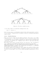
12.2.1 Search Trees . . . . . . . . . .
12.2.2 Variable Selection . . . . . . .
12.2.3 Value Selection . . . . . . . . .
12.2.4 Example . . . . . . . . . . . . .
12.2.5 Counting Backtracks . . . . . .
12.3 Incomplete Tree Search . . . . . . . .
12.3.1 First Solution . . . . . . . . . .
12.3.2 Bounded Backtrack Search . .
12.3.3 Depth Bounded Search . . . .
12.3.4 Credit Search . . . . . . . . . .
12.3.5 Timeout . . . . . . . . . . . . .
12.3.6 Limited Discrepancy Search . .
12.4 Exercises . . . . . . . . . . . . . . . .
.
.
.
.
.
.
.
.
.
.
.
.
.
.
.
.
.
.
.
.
.
.
.
.
.
.
.
.
.
.
.
.
.
.
.
.
.
.
.
.
.
.
.
.
.
.
.
.
.
.
.
.
.
.
.
.
.
.
.
.
.
.
.
.
.
.
.
.
.
.
.
.
.
.
.
.
.
.
.
.
.
.
.
.
.
.
.
.
.
.
.
.
.
.
.
.
.
.
.
.
.
.
.
.
.
.
.
.
.
.
.
.
.
.
.
.
.
.
.
.
.
.
.
.
.
.
.
.
.
.
.
.
.
.
.
.
.
.
.
.
.
.
.
.
.
.
.
.
.
.
.
.
.
.
.
.
.
.
.
.
.
.
.
.
.
.
.
.
.
.
.
.
.
.
.
.
.
.
.
.
.
.
.
.
.
.
.
.
.
.
.
.
.
.
.
.
.
.
.
.
.
.
.
.
.
.
.
.
.
.
.
.
.
.
.
.
.
.
.
.
.
.
.
.
.
.
.
.
.
.
.
.
.
.
.
.
.
.
.
.
.
.
.
.
.
.
.
.
.
.
.
.
.
.
.
.
.
.
.
.
.
.
.
.
.
.
.
.
.
.
.
.
.
.
.
.
.
.
.
.
.
.
.
.
.
.
.
.
.
.
.
.
.
.
.
.
.
.
.
.
.
.
.
.
.
.
.
.
.
.
.
.
.
.
.
.
.
.
.
.
.
.
.
.
.
.
.
.
.
.
.
.
.
.
.
.
.
.
.
.
.
.
.
.
.
.
.
.
.
.
.
.
.
.
.
.
.
.
.
.
.
.
.
.
.
.
.
.
.
.
.
.
.
.
.
.
.
.
.
.
.
.
.
.
.
.
.
.
.
.
.
.
.
.
.
.
.
.
.
.
.
.
.
.
.
.
.
.
.
.
.
.
.
.
.
.
.
.
.
.
.
.
.
.
.
.
.
.
.
.
.
.
113
113
114
116
116
117
117
118
119
119
122
123
124
124
125
126
127
128
129
13 Repair and Local Search
13.1 Motivation . . . . . . . . . . . . . . . . . . . .
13.2 Syntax . . . . . . . . . . . . . . . . . . . . . . .
13.2.1 Setting and Getting Tentative Values .
13.2.2 Building and Accessing Conflict Sets . .
13.2.3 Propagating Conflicts . . . . . . . . . .
13.3 Repairing Conflicts . . . . . . . . . . . . . . . .
13.3.1 Combining Repair with IC Propagation
13.4 Introduction to Local Search . . . . . . . . . .
13.4.1 Changing Tentative Values . . . . . . .
13.4.2 Hill Climbing . . . . . . . . . . . . . . .
13.5 More Advanced Local Search Methods . . . . .
13.5.1 The Knapsack Example . . . . . . . . .
13.5.2 Search Code Schema . . . . . . . . . . .
13.5.3 Random walk . . . . . . . . . . . . . . .
13.5.4 Simulated Annealing . . . . . . . . . . .
13.5.5 Tabu Search . . . . . . . . . . . . . . .
13.6 Repair Exercise . . . . . . . . . . . . . . . . . .
.
.
.
.
.
.
.
.
.
.
.
.
.
.
.
.
.
.
.
.
.
.
.
.
.
.
.
.
.
.
.
.
.
.
.
.
.
.
.
.
.
.
.
.
.
.
.
.
.
.
.
.
.
.
.
.
.
.
.
.
.
.
.
.
.
.
.
.
.
.
.
.
.
.
.
.
.
.
.
.
.
.
.
.
.
.
.
.
.
.
.
.
.
.
.
.
.
.
.
.
.
.
.
.
.
.
.
.
.
.
.
.
.
.
.
.
.
.
.
.
.
.
.
.
.
.
.
.
.
.
.
.
.
.
.
.
.
.
.
.
.
.
.
.
.
.
.
.
.
.
.
.
.
.
.
.
.
.
.
.
.
.
.
.
.
.
.
.
.
.
.
.
.
.
.
.
.
.
.
.
.
.
.
.
.
.
.
.
.
.
.
.
.
.
.
.
.
.
.
.
.
.
.
.
.
.
.
.
.
.
.
.
.
.
.
.
.
.
.
.
.
.
.
.
.
.
.
.
.
.
.
.
.
.
.
.
.
.
.
.
.
.
.
.
.
.
.
.
.
.
.
.
.
.
.
.
.
.
.
.
.
.
.
.
.
.
.
.
.
.
.
.
.
.
.
.
.
.
.
.
.
.
.
.
.
.
.
.
.
.
.
.
.
.
.
.
.
.
.
.
.
.
.
.
.
.
.
.
.
.
.
.
.
.
.
.
.
.
.
.
.
.
.
131
131
131
131
132
133
133
135
137
137
138
139
140
141
141
142
143
145
14 Implementing Constraints
14.1 What is a Constraint in Logic Programming? .
14.2 Background: Constraint Satisfaction Problems
14.3 Constraint Behaviours . . . . . . . . . . . . . .
14.3.1 Consistency Check . . . . . . . . . . . .
14.3.2 Forward Checking . . . . . . . . . . . .
.
.
.
.
.
.
.
.
.
.
.
.
.
.
.
.
.
.
.
.
.
.
.
.
.
.
.
.
.
.
.
.
.
.
.
.
.
.
.
.
.
.
.
.
.
.
.
.
.
.
.
.
.
.
.
.
.
.
.
.
.
.
.
.
.
.
.
.
.
.
.
.
.
.
.
.
.
.
.
.
.
.
.
.
.
.
.
.
.
.
.
.
.
.
.
147
147
148
149
149
150
v
.
.
.
.
.
.
.
.
.
.
.
.
.
.
.
.
.
.
.
.
.
.
.
.
.
.
.
.
.
.
.
.
.
.
.
.
.
.
.
.
.
.
.
.
.
.
.
.
.
.
.
.
.
.
.
.
.
.
.
.
.
.
.
.
.
.
.
.
.
.
.
.
.
.
.
.
.
.
.
.
.
.
.
.
.
.
.
.
.
.
.
.
.
.
.
.
.
.
.
.
.
.
.
.
.
.
.
.
.
.
.
.
.
.
.
.
.
.
.
.
.
.
.
.
.
.
.
.
.
.
.
.
.
.
.
.
.
.
.
.
.
.
.
.
.
.
.
.
.
.
.
.
.
150
151
152
152
152
154
154
155
156
15 Propia and CHR
15.1 Two Ways of Specifying Constraint Behaviours . . .
15.2 The Role of Propia and CHR in Problem Modelling
15.3 Propia . . . . . . . . . . . . . . . . . . . . . . . . . .
15.3.1 How to Use Propia . . . . . . . . . . . . . . .
15.3.2 Propia Implementation . . . . . . . . . . . .
15.3.3 Propia and Related Techniques . . . . . . . .
15.4 CHR . . . . . . . . . . . . . . . . . . . . . . . . . . .
15.4.1 How to Use CHR . . . . . . . . . . . . . . . .
15.4.2 Multiple Heads . . . . . . . . . . . . . . . . .
15.5 A Complete Example of a CHR File . . . . . . . . .
15.5.1 CHR Implementation . . . . . . . . . . . . .
15.6 Global Reasoning . . . . . . . . . . . . . . . . . . . .
15.7 Propia and CHR Exercise . . . . . . . . . . . . . . .
.
.
.
.
.
.
.
.
.
.
.
.
.
.
.
.
.
.
.
.
.
.
.
.
.
.
.
.
.
.
.
.
.
.
.
.
.
.
.
.
.
.
.
.
.
.
.
.
.
.
.
.
.
.
.
.
.
.
.
.
.
.
.
.
.
.
.
.
.
.
.
.
.
.
.
.
.
.
.
.
.
.
.
.
.
.
.
.
.
.
.
.
.
.
.
.
.
.
.
.
.
.
.
.
.
.
.
.
.
.
.
.
.
.
.
.
.
.
.
.
.
.
.
.
.
.
.
.
.
.
.
.
.
.
.
.
.
.
.
.
.
.
.
.
.
.
.
.
.
.
.
.
.
.
.
.
.
.
.
.
.
.
.
.
.
.
.
.
.
.
.
.
.
.
.
.
.
.
.
.
.
.
.
.
.
.
.
.
.
.
.
.
.
.
.
.
.
.
.
.
.
.
.
.
.
.
.
.
159
159
160
162
162
163
165
166
166
167
168
169
170
170
16 The Eplex Library
16.1 Introduction . . . . . . . . . . . . . . . . . . . . . . . . . . . .
16.1.1 What is Mathematical Programming? . . . . . . . . .
16.1.2 Why interface to Mathematical Programming solvers?
16.1.3 Example formulation of an MP Problem . . . . . . . .
16.2 How to load the library . . . . . . . . . . . . . . . . . . . . .
16.3 Modelling MP problems in ECLi PSe . . . . . . . . . . . . . .
16.3.1 Eplex instance . . . . . . . . . . . . . . . . . . . . . .
16.3.2 Example modelling of an MP problem in ECLi PSe . .
16.3.3 Getting more solution information from the solver . .
16.3.4 Adding integrality constraints . . . . . . . . . . . . . .
16.4 Repeated Solving of an Eplex Problem . . . . . . . . . . . . .
16.5 Exercise . . . . . . . . . . . . . . . . . . . . . . . . . . . . . .
.
.
.
.
.
.
.
.
.
.
.
.
.
.
.
.
.
.
.
.
.
.
.
.
.
.
.
.
.
.
.
.
.
.
.
.
.
.
.
.
.
.
.
.
.
.
.
.
.
.
.
.
.
.
.
.
.
.
.
.
.
.
.
.
.
.
.
.
.
.
.
.
.
.
.
.
.
.
.
.
.
.
.
.
.
.
.
.
.
.
.
.
.
.
.
.
.
.
.
.
.
.
.
.
.
.
.
.
.
.
.
.
.
.
.
.
.
.
.
.
.
.
.
.
.
.
.
.
.
.
.
.
173
173
173
174
174
175
176
176
176
178
178
181
185
17 Building Hybrid Algorithms
17.1 Combining Domains and Linear Constraints
17.2 Reasons for Combining Solvers . . . . . . .
17.3 A Simple Example . . . . . . . . . . . . . .
17.3.1 Problem Definition . . . . . . . . . .
17.3.2 Program to Determine Satisfiability
.
.
.
.
.
.
.
.
.
.
.
.
.
.
.
.
.
.
.
.
.
.
.
.
.
.
.
.
.
.
.
.
.
.
.
.
.
.
.
.
.
.
.
.
.
.
.
.
.
.
.
.
.
.
.
187
187
187
188
188
189
14.4
14.5
14.6
14.7
14.8
14.3.3 Domain (Arc) Consistency
14.3.4 Bounds Consistency . . . .
Programming Basic Behaviours . .
14.4.1 Consistency Check . . . . .
14.4.2 Forward Checking . . . . .
Basic Suspension Facility . . . . .
A Bounds-Consistent IC constraint
Using a Demon . . . . . . . . . . .
Exercises . . . . . . . . . . . . . .
.
.
.
.
.
.
.
.
.
.
.
.
.
.
.
.
.
.
vi
.
.
.
.
.
.
.
.
.
.
.
.
.
.
.
.
.
.
.
.
.
.
.
.
.
.
.
.
.
.
.
.
.
.
.
.
.
.
.
.
.
.
.
.
.
.
.
.
.
.
.
.
.
.
.
.
.
.
.
.
.
.
.
.
.
.
.
.
.
.
.
.
.
.
.
.
.
.
.
.
.
.
.
.
.
.
.
.
.
.
.
.
.
.
.
.
.
.
.
.
.
.
.
.
.
.
.
.
.
.
.
.
.
17.4
17.5
17.6
17.7
17.8
17.3.3 Program Performing Optimisation . . . . .
Sending Constraints to Multiple Solvers . . . . . .
17.4.1 Syntax and Motivation . . . . . . . . . . . .
17.4.2 Handling Booleans with Linear Constraints
17.4.3 Handling Disjunctions . . . . . . . . . . . .
17.4.4 A More Realistic Example . . . . . . . . . .
Using Values Returned from the Linear Optimum .
17.5.1 Reduced Costs . . . . . . . . . . . . . . . .
17.5.2 Probing . . . . . . . . . . . . . . . . . . . .
17.5.3 Probing for Scheduling . . . . . . . . . . . .
Other Hybridisation Forms . . . . . . . . . . . . .
References . . . . . . . . . . . . . . . . . . . . . . .
Hybrid Exercise . . . . . . . . . . . . . . . . . . . .
vii
.
.
.
.
.
.
.
.
.
.
.
.
.
.
.
.
.
.
.
.
.
.
.
.
.
.
.
.
.
.
.
.
.
.
.
.
.
.
.
.
.
.
.
.
.
.
.
.
.
.
.
.
.
.
.
.
.
.
.
.
.
.
.
.
.
.
.
.
.
.
.
.
.
.
.
.
.
.
.
.
.
.
.
.
.
.
.
.
.
.
.
.
.
.
.
.
.
.
.
.
.
.
.
.
.
.
.
.
.
.
.
.
.
.
.
.
.
.
.
.
.
.
.
.
.
.
.
.
.
.
.
.
.
.
.
.
.
.
.
.
.
.
.
.
.
.
.
.
.
.
.
.
.
.
.
.
.
.
.
.
.
.
.
.
.
.
.
.
.
.
.
.
.
.
.
.
.
.
.
.
.
.
.
.
.
.
.
.
.
.
.
.
.
.
.
.
.
.
.
.
.
.
.
.
.
.
.
.
.
.
.
.
.
.
.
.
.
.
.
.
.
190
190
190
191
192
193
194
194
196
196
197
198
198
viii
Chapter 1
Introduction
This tutorial provides an introduction to programming in ECLiPSe. It assumes a broad understanding of constrained optimisation problems, some background in mathematical logic and in
programming languages. The tutorial tries to cover most of the basic aspects of using ECLi PSe :
underlying concepts, the programming language, library functionality and interaction with the
system.
A few topics have been left out of this tutorial and are covered elsewhere: The Embedding
Manual explains how to embed ECLi PSe applications into other software environments, and the
Visualisation Manual describes the use of the constraint visualisation facilities. All the features
described in this tutorial are documented in more detail in the ECLi PSe User Manual, Constraint
Library Manual and in particular the Reference Manual. A methodology for developing large
scale applications with ECLi PSe is presented in the document Developing Applications with
ECLi PSe by Simonis.
For an informal introduction to combinatorial optimisation and constraint programming see the
article Constraint Programming1 by Wallace. The most closely related books on the subject
are the textbook Programming with Constraints by Marriott and Stuckey [?] (which contains
ECLi PSe examples), and the seminal book Constraint Satisfaction in Logic Programming [?] by
Van Hentenryck.
A small selection of textbooks on related subjects includes: Foundations of Constraint Satisfaction by Tsang [?], Model Building in Mathematical Programming by Williams [?] and Prolog
Programming for Artificial Intelligence by Bratko [?].
J
References to more detailed documentation are marked like this.
N
Notes that can be skipped on first reading are marked like this.
1
http://www.icparc.ic.ac.uk/eclipse/reports/handbook/handbook.html
1
2
Chapter 2
Getting started with ECLiPSe
2.1
How do I install the ECLi PSe system?
Please see the installation notes that came with ECLi PSe . For Unix/Linux systems, these are
in the file README_UNIX. For Windows, they are in the file README_WIN.TXT.
Please note that choices made at installation time can affect which options are available in the
installed system.
2.2
How do I read the online documentation?
Under Unix, use any HTML browser to open the file doc/index.html in the ECLi PSe installation directory. Under Windows, select the menu entry Start/Programs/ECLiPSe/Documentation.
2.3
How do I run my ECLi PSe programs?
There are two ways of running ECLi PSe programs. The first is using tkeclipse, which provides
an interactive graphical user interface to the ECLi PSe compiler and system. The second is using
eclipse, which provides a more traditional command-line interface. We recommend you use
TkECLi PSe unless you have some reason to prefer a command-line interface.
2.4
2.4.1
How do I use tkeclipse?
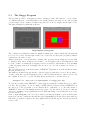
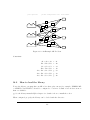
Getting started
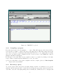
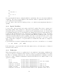
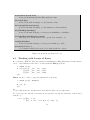
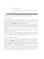
To start TkECLi PSe , either type the command tkeclipse at an operating system commandline prompt, or select TkECLi PSe from the program menu on Windows. This will bring up the
TkECLi PSe top-level, which is shown in Figure 2.1.
Note that help on TkECLi PSe and its component tools is available from the Help menu in the
top-level window.
3
Figure 2.1: TkECLi PSe top-level
2.4.2
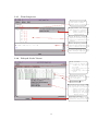
Compiling a program
From the File menu, select the Compile ... option. This will bring up a file selection dialog.
Select the file you wish to compile, and click on the Open button. This will compile the file and
any others it depends on. Messages indicating which files have been compiled and describing
any errors encountered will be displayed in the bottom portion of the TkECLi PSe window
(Output and Error Messages).
If a file has been modified since it was compiled, it may be recompiled by clicking on the make
button. This recompiles any files which have become out-of-date.
J
For more information on program compilation and the compiler, please see The Compiler
chapter in the user manual.
2.4.3
Executing a query
To execute a query, first enter it into the Query Entry text field. You will also need to specify
which module the query should be run from, by selecting the appropriate entry from the dropdown list to the left of the Query Entry field. Normally, the default selection of eclipse will
4
be fine; this will allow access to all ECLi PSe built-ins and all predicates that have not explicitly
been compiled into a different module. Selecting another module for the query is only needed
if you wish to call a predicate which is not visible from the eclipse module, in which case you
need to select that module.
J
For more information about the module system, please see the Module System chapter in
the user manual.
To actually execute the query, either hit the Enter key while editing the query, or click on the
run button. TkECLi PSe maintains a history of commands entered during the session, and these
may be recalled either by using the drop-down list to the right of the Query Entry field, or by
using the up and down arrow keys while editing the Query Entry field.
If ECLi PSe cannot find a solution to the query, it will print No in the Results section of the
TkECLi PSe window. If it finds a solution and knows there are no more, it will print it in the
Results section, and then print Yes. If it finds a solution and there may be more, it will print
the solution found as before, print More, and enable the more button. Clicking on the more
button tells ECLi PSe to try to find another solution. In all cases it also prints the total time
taken to execute the query.
Note that a query can be interrupted during execution by clicking on the interrupt button.
2.4.4
Editing a file
If you wish to edit a file (e.g. a program source file), then you may do so by selecting the
Edit ... option from the File menu. This will bring up a file selection dialog. Select the file
you wish to edit, and click on the Open button.
When you have finished editing the file, save it. After you’ve saved it, if you wish to update the
version compiled into ECLi PSe (assuming it had been compiled previously), simply click on the
make button.
You can change which program is used to edit your file by using the TkECLi PSe Preference
Editor, available from the Tools menu. Alternatively you can use your editor seperately from
ECLi PSe .
2.4.5
Debugging a program
To help diagnose problems in ECLi PSe programs, TkECLi PSe provides the tracer. It is activated
by selecting the Tracer option from the Tools menu. The next time a goal is executed, the
tracer window will become active, allowing you to step through the program’s execution and
examine the program’s state as it executes. A full example is given in chapter 5.
2.4.6
Getting help
More detailed help than is provided here can be obtained online for all the features of TkECLi PSe .
Simply select the entry from the Help menu on TkECLi PSe ’s top-level window which corresponds
to the topic or tool you are interested in.
Detailed documentation about all the predicates in the ECLi PSe libraries can be obtained
through the Library Browser and Help tool. This tool allows you to browse the online help for
5
the ECLi PSe libraries. On the left is a tree display of the libraries available and the predicates
they provide.
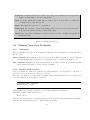
• Double clicking on a node in this tree either expands it or collapses it again.
• Clicking on an entry displays help for that entry to the right.
• Double clicking on a word in the right-hand pane searches for help entries containing that
string.
You can also enter a search string or a predicate specification manually in the text entry box
at the top right. If there is only one match, detailed help for that predicate is displayed. If
there are multiple matches, only very brief help is displayed for each; to get detailed help, try
specifying the module and/or the arity of the predicate in the text field.
Alternatively, you can call the help/1 predicate in the query window (which contains the same
information as the HTML Reference Manual). It has two modes of operation. First, when a
fragment of a built-in name is specified, a list of short descriptions of all built-ins whose name
contains the specified string is printed. For example,
?- help(write).
will print one-line descriptions about write/1, writeclause/2, etc. When a unique specification
is given, the full description of the specified built-in is displayed, e.g. in
?- help(write/1).
or
?- help(ic:alldifferent/1).
2.4.7
Other tools
TkECLi PSe comes with a number of useful tools. Some have been mentioned above, but here is
a more complete list. Note that we only provide brief descriptions here; for more details, please
see the online help for the tool in question.
Compile scratch-pad
This tool allows you to enter small amounts of program code and have it compiled. This is useful
for quick experimentation, but not for larger examples or programs you wish to keep, since the
source code is lost when the session is exited.
Source File Manager
This tool allows you to keep track of and manage which source files have been compiled in the
current ECLi PSe session. You can select files to edit them, or compile them individually, as well
as adding new files.
6
Predicate Browser
This tool allows you to browse through the modules and predicates which have been compiled
in the current session. It also lets you alter some properties of compiled predicates.
Source Viewer
This tool attempts to display the source code for predicates selected in other tools.
Delayed Goals
This tool displays the current delayed goals, as well as allowing a spy point to be placed on the
predicate and the source code viewed.
Inspector
This tool provides a graphical browser for inspecting terms. Goals and data terms are displayed
as a tree structure. Sub-trees can be collapsed and expanded by double-clicking. A navigation
panel can be launched which provides arrow buttons as an alternative way to navigate the tree.
Note that while the inspector window is open, interaction with other TkECLi PSe windows is disallowed. This prevents the term from changing while being inspected. To continue TkECLi PSe ,
the inspector window must be closed.
Global Settings
This tool allows the setting of some global flags governing the way ECLi PSe behaves. See also
the documentation for the set flag/2 and get flag/2 predicates.
Statistics
This tool displays some statistics about memory and CPU usage of the ECLi PSe system, updated at regular intervals. See also the documentation for the statistics/0 and statistics/2
predicates.
Preference Editor
This tool allows you to edit and set various user preferences. This include parameters for how
TkECLi PSe will start up, e.g. the amount of memory it will be able to use, and a initial
query to execute; and parameters which affects the appearance of TkECLi PSe , such as the fonts
TkECLi PSe uses and which editor it launches.
2.5
How do I make things happen at compile time?
A file being compiled may contain queries. These are goals preceded by either the symbol “?-”
or the symbol “:-”. As soon as a query or command is encountered in the compilation of a file,
the ECLi PSe system will try to satisfy it. Thus by inserting goals in this fashion, things can be
made to happen at compile time.
7
In particular, a file can contain a directive to the system to compile another file, and so large
programs can be split between files, while still only requiring a single simple command to compile
them. When this happens, ECLi PSe interprets the pathnames of the nested compiled files
relative to the directory of the parent compiled file; if, for example, the user calls
[eclipse 1]: compile(’src/pl/prog’).
and the file src/pl/prog.pl contains a query
:- [part1, part2].
then the system searches for the files part1.pl and part2.pl in the directory src/pl and not in
the current directory. Usually larger ECLi PSe programs have one main file which contains only
commands to compile all the subfiles. In ECLi PSe it is possible to compile this main file from
any directory. (Note that if your program is large enough to warrant breaking into multiple files
(let alone multiple directories), it is probably worth turning the constituent components into
modules.)
J
See section 4.10 for more information about modules.
How do I use ECLi PSe libraries in my programs?
2.6
A number of files containing library predicates are supplied with the ECLi PSe system. They
are usually installed in an ECLi PSe library directory. These predicates are either loaded automatically by ECLi PSe or may be loaded “by hand”.
During the execution of an ECLi PSe program, the system may dynamically load files containing
library predicates. When this happens, the user is informed by a compilation or loading message.
It is possible to explicitly force this loading to occur by use of the lib/1 or use module/1
predicates. E.g. to load the library called lists, use one of the following goals:
:- lib(lists)
:- use_module(library(lists))
This will load the library file unless it has been already loaded. In particular, a program can
ensure that a given library is loaded when it is compiled, by including an appropriate directive
in the source, e.g. :- lib(lists).
2.7
2.7.1
Other tips
Recommended file names
It is recommended programming practice to give the Prolog source programs the suffix .pl, or
.ecl if it contains ECLi PSe specific code. It is not enforced by the system, but it simplifies
managing the source programs. The compile/1 predicate automatically adds the suffix to the
filename, so that it does not need to be specified; if the literal filename can not be found, the
system tries appending each of the valid suffixes in turn and tries to find the resulting filename.
8
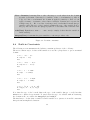
Chapter 3
Prolog Introduction
3.1
Terms and their data types
Prolog data (terms) and programs are built from a small set of simple data-types. In this section,
we introduce these data types together with their syntax (their textual representations). For
the full syntax see the User Manual appendix on Syntax.
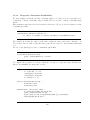
3.1.1
Numbers
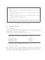
Numbers come in several flavours. The ones that are familiar from other programming languages
are integers and floating point numbers. Integers in ECLi PSe can be as large as fits into the
machine’s memory:
123
0
-27
3492374892749289174
Floating point numbers (represented as IEEE double floats) are written as
0.0 3.141592653589793 6.02e23 -35e-12 -1.0Inf
ECLi PSe
provides two additional numeric types, rationals and bounded reals. ECLi PSe can do
arithmetic with all these numeric types.
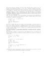
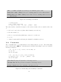
Note that performing arithmetic requires the use of the is/2 predicate:
?- X is 3 + 4.
X = 7
Yes
If one just uses =/2, ECLi PSe will simply construct a term corresponding to the arithmetic
expression, and will not evaluate it:
?- X = 3 + 4.
X = 3 + 4
Yes
J
J
For more details on numeric types and arithmetic in general see the User Manual chapter on
Arithmetic.
For more information on the bounded real numeric type, see Chapter 9.
9
3.1.2
Strings
Strings are a representation for arbitrary sequences of bytes and are written with double quotes:
"hello"
"I am a string!"
"string with a newline \n and a null \000 character"
Strings can be constructed and partitioned in various ways using ECLi PSe primitives.
3.1.3
Atoms
Atoms are simple symbolic constants, similar to enumeration type constants in other languages.
No special meaning is attached to them by the language. Syntactically, all words starting with
a lower case letter are atoms, sequences of symbols are atoms, and anything in single quotes is
an atom:
atom
3.1.4
quark
i486
-*-
???
’Atom’
’an atom’
Lists
A list is an ordered sequence of (any number of) elements, each of which is itself a term. Lists
are delimited by square brackets ([ ]), and elements are separated by a comma. Thus, the
following are lists:
[1,2,3]
[london, cardiff, edinburgh, belfast]
["hello", 23, [1,2,3], london]
A special case is the empty list (sometimes called nil), which is written as
[]
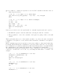
A list is actually composed of head-and-tail pairs, where the head contains one list element, and
the tail is itself a list (possibly the empty list). Lists can be written as a [Head|Tail] pair, with
the head separated from the tail by the vertical bar. Thus the list [1,2,3] can be written in
any of the following equivalent ways:
[1,2,3]
[1|[2,3]]
[1|[2|[3]]]
[1|[2|[3|[]]]]
The last line shows that the list actually consists of 3 [Head|Tail] pairs, where the tail of the
last pair is the empty list. The usefulness of this notation is that the tail can be a variable
(introduced below): [1|Tail], which leaves the tail unspecified for the moment.
10
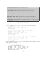
3.1.5
Structures
Structures correspond to structs or records in other languages. A structure is an aggregate of a
fixed number of components, called its arguments. Each argument is itself a term. Moreover, a
structure always has a name (which looks like an atom). The canonical syntax for structures is
<name>(<arg> 1,...<arg> n)
Valid examples of structures are:
date(december, 25, "Christmas")
element(hydrogen, composition(1,0))
flight(london, new_york, 12.05, 17.55)
The number of arguments of a structure is called its arity. The name and arity of a structure are
together called its functor and is often written as name/arity. The last example above therefore
has the functor flight/4.
J
See section 4.1 for information about defining structures with named fields.
Operator Syntax
As a syntactic convenience, unary (1-argument) structures can also be written in prefix or postfix
notation, and binary (2-argument) structures can be written in infix notation, if the programmer
has made an appropriate declaration (called an operator declaration) about its functor. For
example if plus/2 were declared to be an infix operator, we could write:
1 plus 100
instead of
plus(1,100)
It is worth keeping in mind that the data term represented by the two notations is the same,
we have just two ways of writing the same thing. Various logical and arithmetic functors are
automatically declared to allow operator syntax, for example +/2, not/1 etc.
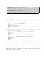
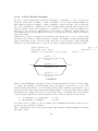
Parentheses
When prefix, infix and postfix notation is used, it is sometimes necessary to write extra parentheses to make clear what the structure of the written term is meant to be. For example to
write the following nested structure
+(*(3,4), 5)
we can alternatively write
3 * 4 + 5
because the star binds stronger than the plus sign. But to write the following differently nested
structure
11
Numbers ECLi PSe has integers, floats, rationals and bounded reals.
Strings Character sequences in double quotes.
Atoms Symbolic constants, usually lower case or in single quotes.
Lists Lists are constructed from cells that have an arbitrary head and a tail which is
again a list.
Structures Structures have a name and a certain number (arity) of arbitrary arguments.
This characteristic is called the functor, and written name/arity.
Figure 3.1: Summary of Data Types
*(3, +(4, 5))
in infix-notation, we need extra parentheses:
3 * (4 + 5)
A full table of the predefined prefix, infix and postfix operators with their relative precedences
can be found in the appendix of the User Manual.
3.2
Predicates, Goals and Queries
Where other programming languages have procedures and functions, Prolog and ECLi PSe have
predicates. A predicate is something that has a truth value, so it is similar to a function with
a boolean result. A predicate definition simply defines what is true. A predicate invocation (or
call) checks whether something is true or false. A simple example is the predicate integer/1,
which has a built-in definition. It can be called to check whether something is an integer:
integer(123)
integer(atom)
integer([1,2])
is true
is false
is false
A predicate call like the above is also called a goal. A starting goal that the user of a program
provides is called a query. To show queries and their results, we will from now on use the
following notation:
?- integer(123).
Yes.
?- integer(atom).
No.
?- integer([1,2]).
No.
A query can simply be typed at the eclipse prompt, or entered into the query field in a tkeclipse
window. Note that it is not necessary to enter the ?- prefix. On a console input, is however
12
necessary to terminate the query with a full-stop (a dot followed by a newline). After executing
the query, the system will print one of the answers Yes or No.
3.2.1
Conjunction and Disjunction
Goals can be combined to form conjunctions (AND) or disjunctions (OR). Because this is so
common, Prolog uses the comma for AND and the semicolon for OR. The following shows two
examples of conjunction, the first one is true because both conjuncts are true, the second is false:
?- integer(5), integer(7).
Yes.
?- integer(5), integer(hello).
No.
In contrast, a disjunction is only false if both disjuncts are false:
?- ( integer(5) ; integer(hello) ).
Yes.
?- ( integer(hello) ; integer(world) ).
No.
As in this example, it is advisable to always surround disjunctions with parentheses. While not
strictly necessary in this example, they are often required to clarify the structure.
3.3
Unification and Logical Variables
3.3.1
Symbolic Equality
Prolog has a particularly simple idea of equality, namely structural equality by pattern matching. This means that two terms are equal if and only if they have exactly the same structure.
No evaluation of any kind is perfomed on them:
?- 3 = 3.
Yes.
?- 3 = 4.
No.
?- hello = hello.
Yes.
?- hello = 3.
No.
?- foo(a,2) = foo(a,2).
Yes.
?- foo(a,2) = foo(b,2).
No.
?- foo(a,2) = foo(a,2,c).
No.
?- foo(3,4) = 7.
13
No.
?- +(3,4) = 7.
No.
?- 3 + 4 = 7.
No.
Note in particular the last two examples (which are equivalent): there is no automatic arithmetic
evaluation. The term +(3,4) is simply a data structure with two arguments, and therefore of
course different from any number.
Note also that we have used the built-in predicate =/2, which exactly implements this idea of
equality.
3.3.2
Logical Variables
So far we have only performed tests, giving only Yes/No results. How can we compute more
interesting results? The solution is to introduce Logical Variables. It is very important to
understand that Logical Variables are variables in the mathematical sense, not in the usual
programming language sense. Logical Variables are simply placeholders for values which are not
yet known, like in mathematics. In conventional programming languages on the other hand,
variables are labels for storage locations. The important difference is that the value of a logical
variables is typically unknown at the beginning, and only becomes known in the course of the
computation. Once it is known, the variable is just an alias for the value, i.e. it refers to a term.
Once a value has be assigned to a logical variable, it remains fixed and cannot be assigned a
different value.
Logical Variables are written beginning with an upper-case letter or an underscore, for example
X
Var
Quark
_123
R2D2
If the same name occurs repeatedly in the same input term (e.g. the same query or clause), it
means the same variable.
3.3.3
Unification
With logical variables, the above equality tests become much more interesting, resulting in the
concept of Unification. Unification is an extension of the idea of pattern matching of two terms.
In addition to matching, unification also causes the binding (instantiation, aliasing) of variables
in the two terms. Unification instantiates variables such that the two unified terms become
equal. For example
X = 7
X = Y
foo(X) =
foo(X,Y)
foo(X,4)
foo(X) =
foo(X,X)
foo(7)
= foo(3,4)
= foo(3,Y)
foo(Y)
= foo(3,4)
is
is
is
is
is
is
is
true with X instantiated to 7
true with X instantiated to Y (or vice versa)
true with X instantiated to 7
true with X instantiated to 3 and Y to 4
true with X instantiated to 3 and Y to 4
true with X instantiated to Y (or vice versa)
false because there is no possible value for X
14
Predicate Something that is true or false, depending on its definition and its arguments.
Defines a relationship between its arguments.
Goal A logical formula whose truth value we want to know. A goal can be a conjunction
or disjunction of other (sub-)goals.
Query The initial Goal given to a computation.
Unification An extension of pattern matching which can bind logical variables (placeholders) in the matched terms to make them equal.
Clause One alternative definition for when a predicate is true. A clause is logically an
implication rule.
Figure 3.2: Basic Terminology
3.4
Defining Your Own Predicates
3.4.1
Comments
Since we will annotate some of our programs, we first introduce the syntax for comments. There
are two types:
Block comment The comment is enclosed between the delimiters /* and */. Such comments
can span multiple lines, and may be conveniently used to comment out unused code.
Line comment Anything following and including ’%’ in a line is taken as a comment (unless
the ’%’ character is part of a quoted atom or string).
3.4.2
Clauses and Predicates
Prolog programs are built from valid Prolog data-structures. A program is a collection of
predicates, and a predicate is a collection of clauses.
The idea of a clause is to define that something is true. The simplest form of a clause is the
fact. For example, the following two are facts:
capital(london, england).
brother(fred, jane).
Syntactically, a fact is just a structure (or an atom) terminated by a full stop.
Generally, a clause clause has the form
Head :- Body.
where Head is a structure (or atom) and Body is a Goal, possibly with conjunctions and disjunctions like the query discussed above. The following is a clause
15
uncle(X,Z) :- brother(X,Y), parent(Y,Z).
Logically, this can be read as a reverse implication
uncle(X, Z) ←− brother(X, Y ) ∧ parent(Y, Z)
or, more precisely
∀X∀Z : uncle(X, Z) ←− ∃Y : brother(X, Y ) ∧ parent(Y, Z)
stating that uncle(X,Z) is true if brother(X,Y) and parent(Y,Z) are true. Note that a fact is
equivalent to a clause where the body is true:
brother(fred, jane) :- true.
One or multiple clauses with the same head functor (same name and number of arguments)
together form the definition of a predicate. Logically, multiple clauses are read as a disjunction,
i.e. they define alternative ways in which the predicate can be true. The simplest case is a
collection of alternative facts:
parent(abe, homer).
parent(abe, herbert).
parent(homer, bart).
parent(marge, bart).
The following defines the ancestor/2 predicate by giving two alternative clauses (rules):
ancestor(X,Y) :- parent(X,Y).
ancestor(X,Y) :- parent(Z,Y), ancestor(X,Z).
Remember that a clause can be read logically, with the :- taking the meaning of implication,
and the comma separating goals read as a conjunction. The logical reading for several clauses
of the same predicate is disjunction between the clauses. So the first ancestor rule above states
that if X is a parent of Y, then this implies that X is an ancestor of Y. The second rule, which
specifies another way X can be an ancestor of Y states that if some other person, Z, is the parent
of Y, and X is an ancestor of Z, then this implies that X is also an ancestor of Y.
N
It is also important to remember that the scope of a variable name only extends over the
clause in which it is in, so any variables with the same name in the same clause refer to
the same variable, but variables which occur in different clauses are different even if they
have been written with the same name.
16
1. Pick one (usually the leftmost) goal from the resolvent. If the resolvent is empty,
stop.
2. Find all clauses whose head successfully unifies with this goal. If there is no such
clause, go to step 6.
3. Select the first of these clause. If there are more, remember the remaining ones. This
is called a choice point.
4. Unify the goal with the head of the selected clause. (this may instantiate variables
both in the goal and in the clause’s body).
5. Prefix this clause body to the resolvent and go to 1.
6. Backtrack: Reset the whole computation state to how it was when the most recent
choice point was created. Take the clauses remembered in this choice point and go
to 3.
Figure 3.3: Execution Algorithm
3.5
Execution Scheme
3.5.1
Resolution
Resolution is the computation rule used by Prolog. Given a set of facts and rules as a program,
execution begins with a query, which is an initial goal that is to be resolved. The set of goals
that still have to be resolved is called the resolvent.
Consider again the ancestor/2 and parent/2 predicate shown above.
ancestor(X,Y) :- parent(X,Y).
ancestor(X,Y) :- parent(Z,Y), ancestor(X,Z).
% clause 1
% clause 2
parent(abe, homer).
parent(abe, herbert).
parent(homer, bart).
parent(marge, bart).
%
%
%
%
clause
clause
clause
clause
3
4
5
6
Program execution is started by issuing a query, for example
?- ancestor(X, bart).
This is our initial resolvent. The execution mechanism is now as follows: In our example, the
Prolog system would attempt to unify ancestor(X, bart) with the program’s clause heads.
Both clauses of the ancestor/2 predicate can unify with the goal, but the textually first clause,
clause 1, is selected first, and successfully unified with the goal:
17
Goal (Query):
Selected:
Unifying:
results in:
New resolvent:
More choices:
ancestor(X,bart)
clause 1
ancestor(X,bart) = ancestor(X1,Y1)
X=X1, Y1=bart
parent(X, bart)
clause 2
The body goal of clause 1 parent(X, bart) is added to the resolvent, and the system remembers
that there is an untried alternative – this is referred to as a choice-point.
In the same way, parent(X, bart) is next selected for unification. Clauses 5 and 6 are possible
matches for this goal, with clause 5 selected first. There are no body goals to add, and the
resolvent is now empty:
Goal:
Selected:
Unifying:
results in:
New resolvent:
More choices:
parent(X, bart)
clause 5
parent(X,bart) = parent(homer,bart)
X = homer
clause 6, then clause 2
The execution of a program completes successfully when there is an empty resolvent. The
program has thus found the first solution to the query, in the form of instantiations to the
original Query’s variables, in this case X = homer. ECLi PSe returns this solution, and also asks
if we want more solutions:
?- ancestor(X,bart).
X = homer
More? (;)
Responding with ’;’ will cause ECLi PSe to try to find alternative solutions by backtracking to
the most recent choice-point, i.e. to seek an alternative to parent/2. Any bindings done during
and after the selection of clause 5 are undone, i.e. the binding of X to homer is undone. Clause
6 is now unified with the goal parent(X,Y), which again produces a solution:
Goal:
Selected:
Unifying:
results in:
New resolvent:
More choices:
parent(X, bart)
clause 6
parent(X,bart) = parent(marge,bart)
X = marge
clause 2
If yet further solutions are needed, then ECLi PSe would again backtrack. This time, parent/2
no longer have any alternatives left to unify, so the next older choice-point, the one made for
ancestor/2, is the one that would be considered. The computation is returned to the state it
was in just before clause 1 was selected, and clause 2 is unified with the query goal:
Goal:
Selected:
Unifying:
ancestor(X,bart)
clause 2
ancestor(X,bart) = ancestor(X1,Y1)
18
results in:
New resolvent:
More choices:
Y1 = bart, X1 = X
parent(Z1, bart), ancestor(X1, Z1)
For the first time, there are more than one goal in the resolvent, the leftmost one, parent(Z1,bart) is then selected for unification. Again, clauses 5 and 6 are candidates, and a
new choice-point is created, and clause 5 tried first.
Goal:
Selected:
Unifying:
results in:
New resolvent:
More choices:
parent(Z1, bart)
clause 5
parent(Z1, bart) = parent(homer, bart)
Z1 = homer
ancestor(X1, homer)
clause 6
Eventually, after a few more steps (via finding the ancestor of homer), this leads to a new
solution, with abe returned as an ancestor of bart:
?- ancestor(X,bart).
X = abe
More? (;)
If yet more solutions are requested, then because only one parent for homer is given by the
program, ECLi PSe would backtrack to the only remaining choice-point, unifying clause 6 is
unified with the goal, binding Z1 to marge. However, no ancestor for marge can be found,
because no parent of marge is specified in the program. No more choice-points remains to be
tried, so the execution terminates.
3.6
Partial data structures
Logical variables can occur anywhere, not only as arguments of clause heads and goals, but
also within data structures. A data structure which contains variables is called a partial data
structure, because it will eventually be completed by substituting the variable with an actual
data term. The most common case of a partial data structure is a list whose tail is not yet
instantiated.
Consider first an example where no partial lists occur. In the following query, a list is built
incrementally, starting from its end:
?L1
L2
L3
L4
L1 = [], L2 = [c|L1], L3 = [b|L2], L4 = [a|L3].
= []
= [c]
= [b, c]
= [a, b, c]
Whenever a new head/tail cell is created, the tail is already instantiated to a complete list.
But is is also possible to build the list from the front. The following code, in which the goals
have been reordered, gives the same final result as the code above:
19
?L1
L2
L3
L4
L4 = [a|L3], L3 = [b|L2], L2 = [c|L1], L1 = [].
= []
= [c]
= [b, c]
= [a, b, c]
However, in the course of the computation, variables get instantiated to ”partial lists”, i.e. lists
whose head is known, but whose tail is not. This is perfectly legal: due to the nature of the
logical variable, the tail can be filled in later by instantiating the variable.
3.7
More control structures
3.7.1
Disjunction
Disjunction is normally specified in Prolog by different clauses of a predicate, but it can also be
specified within a single clause by the use of ;/2. For example,
atomic_particle(X) :- (X = proton ; X = neutron ; X = electron).
This is logically equivalent to:
atomic_particle(proton).
atomic_particle(neutron).
atomic_particle(electron).
3.7.2
Conditional
Conditionals can be specified using the ->/2 operator. In combination with ;/2, a conditional
similar to ‘if-then-else’ constructs of conventional language can be constructed: X->Y;Z, where
X, Y and Z can be one or more goals, means that if X is true, then Y will be executed, otherwise
Z. Only the first solution of X is explored, so that on backtracking, no new solutions for X will
be tried. In addition, if X succeeds, then the ‘else’ part, Z will never be tried. If X fails, then the
‘then’ part, Y, will never be tried. An example of ‘if-then-else’ is:
max(X,Y, Max) :number(X), number(Y),
(X > Y -> Max = X ; Max = Y).
where Max is the bigger of the numbers X or Y. Note the use of the brackets to make the scope
of the if-then-else clear and correct.
20
3.7.3
Call
One feature of Prolog is the equivalence of programs and data – both are represented as terms.
The predicate call allows program terms (i.e. data) to be treated as goals: call(X) will cause
X to be treated as a goal and executed. Although at the time when the predicate is executed,
X has to be instantiated, it does not need to be instantiated (or even known) at compile time.
For example, it is possible to define disjunction (;) as follows:
X ; Y :- call(X).
X ; Y :- call(Y).
3.7.4
All Solutions
In the pure computational model of Prolog, alternative solutions are computed one-by-one on
backtracking. Only one solution is available at any time, while previous solutions disappear on
backtracking:
?- weekday(X).
X = mo
More
X = tu
More
X = we
More
...
Sometimes it is useful to have all solution together in a list. This can be achieved by using one
of the all-solutions predicates findall/3, setof/3 or bagof/3:
?- findall(X, weekday(X), List).
X = X
List = [mo, tu, we, th, fr, sa, su]
Yes
J
For the differences between findall/3, setof/3 and bagof/3 see the ECLi PSe Reference Manual.
3.8
Using Cut
Cut (written as !) prunes away part of the Prolog search-space. This can be a very powerful
mechanism for improving the performance of programs, and even the suppression of unwanted
solutions. However, it can also be easily misused and over-used.
Cut does two things:
commit Disregard any later clauses for the predicate.
prune Throw away all alternative solutions to the goals to the left of the cut.
21
3.8.1
Commit to current clause
Consider the following encoding of the “minimum” predicate:
min(X,Y, Min) :- X <Y, Min = X.
min(X,Y, Min) :- Y=<X, Min = Y.
Whilst logically correct, the behaviour of this encoding is non-optimal for two reasons. Consider
the goal :- min(2,3,M). Although the first clause succeeds, correctly instantiating M to 2,
Prolog leaves an open choice point. If these clauses and goal occur as part of a larger program
and goal, a failure might occur later, causing backtracking. Prolog would then, vainly, try to
find another minimum using the second clause for min. Firstly the open choice point costs space,
and the secondly the unsuccessful evaluation of the second clause costs execution time.
To achieve the same logic, but more efficient behaviour, the programmer can introduce a cut.
For example min is typically encoded as follows:
min(X,Y, Min) :- X<Y, !, Min = X.
min(X,Y, Y).
The cut removes the unnecessary choice point and test.
3.8.2
Prune alternative solutions
A cut may occur anywhere where a goal may occur, consider the following:
first_prime(X, P) :prime(X,P), !.
where first_prime returns the first prime number smaller than X. In this case, it calls a predicate
prime/2, which generates prime numbers smaller than X, starting from the largest one. The effect
of the cut here is to prune away all the remaining solutions to prime(X,P) once the first one is
generated, so that on backtracking, prime(X,P) is not tried for alternative solutions. The cut
will also commit the execution to this clause for first_prime/2, but as there is only one clause,
this has no visible effect.
3.9
Common Pitfalls
Prolog is different from conventional programming languages, and a common problem is to
program Prolog like a conventional language. Here are some points to note:
• Unification is more powerful than normal case discrimination (see section 3.9.1);
• Prolog procedure calls are more powerful than conventional procedure calls. In particular,
backtracking is possible (see section 3.9.2);
22
3.9.1
Unification works both ways
One common problem is to write a predicate expecting certain instantiation patterns for the
arguments, and then get unexpected results when the arguments do not conform to the expected
pattern. An example is the member relation, intended to check if an item Item is a member of
a list or not. This might be written as:
member(Item, [Item|_]).
member(Item, [_|List]) :- member(Item, List).
The expected usage assumes both Item and the list are ground. In such cases, the above predicate
does indeed check if Item occurs in the list given as a second argument. However, if either of the
arguments are not ground, then potentially unexpected behaviour might occur. Consider the
case where Item is a variable, then the above predicate will enumerate the elements of the list
successively through backtracking. On the other hand, if any of the list elements of the list is
a variable, they would be unified with Item. Other instantiation patterns for either arguments
can produce even more complex results.
If the intended meaning is simply to check if Item is a member of a list, this can be done by:
% is_member(+Element, +List)
% check if Element is an element that occurs in a List of
% ground elements
is_member(Item, [Element|_]) :- Item == Element.
is_member(Item, [_|List]) :- nonvar(List), is_member(Item, List).
Note the use of comments to make clear the intention of the use of the predicate. The convention
used is that ‘+’ indicates that an argument should be instantiated (i.e. not a variable), ‘-’ for an
argument that should be an uninstantiated variable, and ’ ?’ indicates that there is no restrictions
on the mode of the argument.
3.9.2
Unexpected backtracking
Remember that when coding in Prolog, any predicate may be backtracked into. So correctness
in Prolog requires:
• Predicate returns the correct answer when first called.
• Predicate behaves correctly when backtracked into.
Recall that backtracking causes alternative choices to be explored, if there are any. Typically
another choice corresponds to another clause in the poredicate definition, but alternative choices
may come from disjunction (see above) or built-in predicates with multiple (alternative) solutions. The programmer should make sure that a predicate will only produce those solutions that
23
are wanted. Excess alternatives can be removed by coding the program not to produce them,
or by the cut, or the conditional.
For example, to return only the first member, in the is_member/2 example, the predicate can
be coded using the cut, as follows:
is_member(Item, [Element|_]) :- Item == Element, !.
is_member(Item, [_|List]) :- nonvar(List), is_member(Item, List).
Using conditional
Another way to remove excess choice points is the conditional:
is_member(Item, [Element|List]) :( Item == Element ->
true
;
nonvar(List), is_member(Item, List)
).
3.10
Exercises
1. Consider again the “family tree” example (see Section 3.4.2). As well as the parent/2
predicate, suppose we have a male/1 predicate as follows:
male(abe).
male(homer).
male(herbert).
male(bart).
Define a brother/2 predicate, expressed just in terms of parent/2 and male/1. Make
sure Homer is not considered his own brother.
2. Consider the following alternative definition of ancestor/2:
ancestor(X, Y) :- parent(X, Y).
ancestor(X, Y) :- ancestor(X, Z), parent(Z, Y).
What is wrong with this code? What happens if you use it to find out who Bart is an
ancestor of?
24
Chapter 4
ECLiPSe Programming
4.1
Structure Notation
In ECLi PSe , structure fields can be given names. This makes it possible to write structures in
a more readable and maintainable way. Such structures first need to be declared by specifying
a template like:
:- local struct( book(author, title, year, publisher) ).
Structures with the functor book/4 can then be written as
book with []
book with title:’tom sawyer’
book with [title:’tom sawyer’, year:1876, author:twain]
which, in canonical syntax, correspond to the following:
book(_, _, _, _)
book(_, ’tom sawyer’, _, _)
book(twain, ’tom sawyer’, 1876, _)
There is absolutely no semantic difference between the two syntactical forms. The with-syntax
with names has the advantage that
• the arguments can be written in any order
• “dummy” arguments with anonymous variables do not need to be written
• the arity of the structure is not implied (and can be changed by changing the declaration
and recompiling the program)
Sometimes it is necessary to refer to the numerical position of a structure field within the
structure, e.g. in the arg/3 predicate:
arg(3, B, Y)
25
When the structure has been declared as above, we can write instead:
arg(year of book, B, Y)
Declared structures help readability, and make programs easier to modify. In order not to lose
these benefits, one should always use with- and of-syntax when working with them, and never
write them in canonical syntax or referring to argument positions numerically.
J
See also the update struct/4 built-in predicate.
4.2
Loops
To reduce the need for auxiliary recursive predicates, ECLi PSe allows the use of an iteration
construct
( IterationSpecs do Goals )
Typical applications are: Iteration over a list
?- ( foreach(X,[1,2,3]) do writeln(X) )
1
2
3
Yes (0.00s cpu)
Process all elements of one list and construct another:
?- ( foreach(X,[1,2,3]), foreach(Y,List) do Y is X+3 ).
List = [4, 5, 6]
Yes (0.00s cpu)
Process a list to compute the sum of its elements:
?- ( foreach(X,[1,2,3]), fromto(0,In,Out,Sum) do Out is In+X ).
Sum = 6
Yes (0.00s cpu)
Note that the variables X, Y, In and Out are local variables in the loop, while the input list and
Sum are shared with the context.
If a parameter remains constant across all loop iterations it must be specified explicitly (via
param), for example when iterating over an array:
?- Array = [](4,3,6,7,8),
(
for(I,1,5),
fromto(0,In,Out,Sum),
param(Array)
do
Out is In + Array[I]
).
J
For details and more examples see the description of the do/2 built-in predicate. Additional
background can be found in [?].
26
fromto(First,In,Out,Last)
iterate Goals starting with In=First until Out=Last.
foreach(X,List)
iterate Goals with X ranging over all elements of List.
foreacharg(X,StructOrArray)
iterate Goals with X ranging over all arguments of StructOrArray.
for(I,MinExpr,MaxExpr)
iterate Goals with I ranging over integers from MinExpr to MaxExpr.
for(I,MinExpr,MaxExpr,Increment)
same as before, but Increment can be specified (it defaults to 1).
count(I,Min,Max)
iterate Goals with I ranging over integers from Min up to Max.
param(Var1,Var2,...)
for declaring variables in Goals global, ie shared with the context.
Figure 4.1: Iteration Specifiers for Loops
4.3
Working with Arrays of Items
For convenience, ECLi PSe has some features for facilitating working with arrays of items. Arrays
can be of any dimension, and can be declared with the dim/2 predicate:
?- dim(M,[3,4]).
M = []([](_131, _132, _133, _134),
[](_126, _127, _128, _129),
[](_121, _122, _123, _124))
yes.
dim/2 can also be used to query the dimensions of an array:
?- dim(M,[3,4]), dim(M,D).
...
D = [3, 4]
yes.
N
Note that arrays are just structures, and that the functor is not important.
To access a specific element of an array in an expression, specify the index list of the desired
element, e.g.
?- M = []([](2, 3, 5),
[](1, 4, 7)),
X is M[1, 2] + M[2, 3].
27
• Arrays are just structures
• The functor is not important
• Declare or query array size with dim/2
• Access elements in expressions by specifying their index list (e.g. A[7], M[2,3])
• Indices start at 1
Figure 4.2: Array notation
X = 10
M = []([](2, 3, 5), [](1, 4, 7))
yes.
J
For further details see the Array Notation section of the User Manual.
4.4
Storing Information Across Backtracking
In pure logic programming, the complete state of a computation is reset to an earlier state on
backtracking. The all-solutions predicates introduced in section 3.7.4 provide a way to collect
solutions across backtracking.
The following section presents ECLi PSe ’s lower-level primitives for storing information across
failures: bags and shelves. Both bags and shelves are referred to by handle, not by name,
so they make it easy to write robust, reentrant code. Bags and shelves disappear when the
system backtracks over their creation, when the handle gets garbage collected, or when they are
destroyed explicitly.
4.4.1
Bags
A bag is an anonymous object which can be used to store information across failures. A typical
application is the collection of alternative solutions.
A bag is an unordered collection, referred to by a handle. A bag is created using bag create/1,
terms can be added to a bag using bag enter/2, and the whole contents of the bag can be
retrieved using bag retrieve/2 or bag dissolve/2. A simple version of the findall/3 predicate
from section 3.7.4 can be implemented like:
simple_findall(Goal, Solutions) :bag_create(Bag),
(
call(Goal),
bag_enter(Bag, Goal),
fail
28
;
bag_dissolve(Bag, Solutions)
).
4.4.2
Shelves
A shelf is an anonymous object which can be used to store information across failures. A typical
application is counting of solutions, keeping track of the best solution, aggregating information
across multiple solutions etc.
A shelf is an object with multiple slots whose contents survive backtracking. The content of
each slot can be set and retrieved individually, or the whole shelf can be retrieved as a term.
Shelves are referred to by a handle.
A shelf is initialized using shelf create / 2 or shelf create / 3. Data is stored in the slots (or the
shelf as a whole) with shelf set / 3 and retrieved with shelf get / 3.
For example, here is a meta-predicate to count the number of solutions to a goal:
count_solutions(Goal, Total) :shelf_create(count(0), Shelf),
(
call(Goal),
shelf_get(Shelf, 1, Old),
New is Old + 1,
shelf_set(Shelf, 1, New),
fail
;
shelf_get(Shelf, 1, Total)
),
shelf_abolish(Shelf).
4.5
Input and Output
4.5.1
Printing ECLi PSe Terms
The predicates of the write-group are generic in the sense that they can print any ECLi PSe
data structure. The different predicates print slightly different formats. The write/1 predicate is intended to be most human-readable, while writeq/1 is designed so that the printed
data can be read back by the predicates of the read-family. If we print the structured term
foo(3+4, [1,2], X, ’a b’, "string") the results are as follows:
write:
writeq:
foo(3 + 4, [1, 2], X, a b, string)
foo(3 + 4, [1, 2], _102, ’a b’, "string")
The write-format is the shortest, but some information is missing, e.g. that the sequence a b is
an atomic unit and that string is a string and not an atom. The writeq-format quotes items
29
write(+Stream, ?Term)
write one term in a default format.
write term(+Stream, ?Term, +Options)
write one term, format options can be selected.
printf(+Stream, +Format, +ArgList)
write a string with embedded terms, according to a format string.
writeq(+Stream, ?Term), write canonical(+Stream, ?Term)
write one term so that it can be read back.
put(+Stream, +Char)
write one character.
Figure 4.3: Builtins for writing
properly, moreover, the variables are printed with unique numbers, so different variables are
printed differently and identical ones identically.
Single characters, encoded in ascii, can be output using put/1, for example:
[eclipse: 1] put(97).
a
yes.
4.5.2
Reading ECLi PSe Terms
If the data to be read is in Prolog syntax, it can be read using read(?Term). This predicate
reads one fullstop-terminated ECLi PSe term from stream Stream. A fullstop is defined as a dot
followed by a layout character like blank space or newline. Examples:
[eclipse 4]: read(X).
123,a.
X = 123, a
yes.
[eclipse 6]: read(X).
[3,X,foo(bar),Y].
X = [3, X, foo(bar), Y]
yes.
Single characters can be input using get/1, which gets their ascii encoding, for example:
[eclipse: 1] get(X).
a
X=97
yes.
30
read(+Stream, -Term)
read one fullstop-terminated ECLi PSe term.
read term(+Stream, -Term, +Options)
read one fullstop-terminated ECLi PSe term.
get(+Stream, -Char)
read one character.
read string(+Stream, +Terminator, -Length, -String)
read a string up to a certain terminator character.
read token(+Stream, -Token, -Class)
read one syntactic token (e.g. a number, an atom, a bracket, etc).
Figure 4.4: Builtins for reading
4.5.3
Formatted Output
The printf-predicate is similar to the printf-function in C, with some ECLi PSe -specific format
extensions. Here are some examples of printing numbers:
?- printf("%d", [123]).
123
yes.
?- printf("%5d,%05d", [123,456]).
123,00456
yes.
?- printf("%6.2f", [123]).
type error in printf("%6.2f", [123])
?- printf("%6.2f", [123.4]).
123.40
yes.
?- printf("%6.2f", [12.3]).
12.30
yes.
The most important ECLi PSe -specific format option is %w, which allows to print like the predicates of the write-family:
?- printf("%w", [foo(3+4, [1,2], X, ’a b’, "string")]).
foo(3 + 4, [1, 2], X, a b, string)
The %w format allows a number of modifiers in order to access all the existing options for the
printing of ECLi PSe terms.
J
For details see the write term/2 and printf/2 predicates.
31
I/O device
tty
file
string
queue
pipe
socket
null
How to open
implicit (stdin,stdout,stderr) or open/3 of a device file
open(FileName, Mode, Stream)
open(string(String), Mode, Stream)
open(queue(String), Mode, Stream)
exec/2, exec/3 and exec group/3
socket/3 and accept/3
implicit (null stream)
Figure 4.5: How to open streams onto the different I/O devices
4.5.4
Streams
ECLi PSe I/O is done from and to named channels called streams. The following streams are
always opened when ECLi PSe is running: input (used by the input predicates that do not have
an explicit stream argument, e.g. read/1 ), output (used by the output predicates that do
not have an explicit stream argument, e.g. write/1 ), error (output for error messages and all
messages about exceptional states ), warning output (used by the system to output warning
messages ), log output (used by the system to output log messages, e.g. messages about garbage
collection activity ), null ( a dummy stream, output to it is discarded, on input it always gives
end of file).
Data can be read from a specific stream using read(+Stream, ?Term), and written to a
specific stream using write(+Stream, ?Term). If no particular stream is specified, input
predicates read from input and output predicates write to output.
New streams may be opened onto various I/O devices, see figure 4.5.
All types of streams are closed using close(+Stream).
J
See the complete description of the stream-related built-in predicates in the Reference Manual
For network communication over sockets, there is a full set of predicates modelled after the BSD
socket interface: socket/3, accept/3, bind/2, listen/2, select/3. See the reference manual
for details.
Output in ECLi PSe is usually buffered, i.e. printed text goes into a buffer and may not immediately appear on the screen, in a file, or be sent via a network connection. Use flush(+Stream)
to empty the buffer and write all data to the underlying device.
4.6
Matching
In ECLi PSe you can write clauses that use matching (or one-way unification) instead of head
unification. Such clauses are written with the ?- functor instead of :-. Matching has the property
that no variables in the caller will be bound. For example
p(f(a,X)) ?- writeln(X).
32
will fail for the following calls:
?- p(F).
?- p(f(A,B)).
?- p(f(A,b)).
and succeed (printing b) for
?- p(f(a,b)).
Moreover, the clause
q(X,X) ?- true.
will fail for the calls
????-
q(a,b).
q(a,B).
q(A,b).
q(A,B).
and succeed for
?- q(a,a).
?- q(A,A).
33
4.7
List processing
Lists are probably the most heavily used data structure in Prolog and ECLi PSe . Apart from unification/matching, the most commonly used list processing predicates are: append/3, length/2,
member/2 and sort/2. The append/3 predicate can be used to append lists or to split lists:
?- append([1, 2], [3, 4], L).
L = [1, 2, 3, 4]
Yes (0.00s cpu)
?- append(A, [3, 4], [1, 2, 3, 4]).
A = [1, 2]
More (0.00s cpu)
No (0.01s cpu)
?- append([1, 2], B, [1, 2, 3, 4]).
B = [3, 4]
Yes (0.00s cpu)
The length/2 predicate can be used to compute the length of a list or to construct a list of a
given length:
?- length([1, 2, 3, 4], N).
N = 4
Yes (0.00s cpu)
?- length(List, 4).
List = [_1693, _1695, _1697, _1699]
Yes (0.00s cpu)
The member/2 predicate can be used to check membership in a list (but memberchk/2 should
be preferred for that purpose), or to backtrack over all list members:
?- memberchk(2, [1, 2, 3]).
Yes (0.00s cpu)
?- member(X, [1, 2, 3]).
X = 1
More (0.00s cpu)
X = 2
More (0.01s cpu)
X = 3
Yes (0.01s cpu)
The sort/2 predicate can sort any list and remove duplicates:
?- sort([5, 3, 4, 3, 2], Sorted).
Sorted = [2, 3, 4, 5]
Yes (0.00s cpu)
J
For more list processing utilities, see the documentation for library(lists).
34
4.8
String processing
ECLi PSe (unlike many Prolog systems) provides a string data type and the corresponding string
manipulation predicates, e.g. string length/2, concat string/2, split string/4, substring/4, and
conversion from and to other data types, e.g. string list/2, atom string/2, number string/2,
term string/2.
?- string_length("hello", N).
N = 5
Yes (0.00s cpu)
?- concat_string([abc, 34, d], S).
S = "abc34d"
Yes (0.00s cpu)
?- string_list("hello", L).
L = [104, 101, 108, 108, 111]
Yes (0.00s cpu)
?- term_string(foo(3, bar), S).
S = "foo(3, bar)"
Yes (0.00s cpu)
4.9
Term processing
Apart from unification/matching, there are a number of generic built-in predicates that work
on arbitrary data terms. The =.. predicate converts structures into lists and vice versa:
?- foo(a, b, c) =.. List.
List = [foo, a, b, c]
Yes (0.00s cpu)
?- Struct =.. [foo, a, b, c].
Struct = foo(a, b, c)
Yes (0.00s cpu)
The arg/3 predicate extracts an argument from a structure:
?- arg(2, foo(a, b, c), X).
X = b
Yes (0.00s cpu)
The functor/3 predicate extracts functor name and arity from a structured term, or, conversely,
creates a structured term with a given functor name and arity:
?- functor(foo(a, b, c), N, A).
N = foo
A = 3
Yes (0.00s cpu)
?- functor(F, foo, 3).
F = foo(_1696, _1697, _1698)
Yes (0.00s cpu)
35
The term variables/2 predicate extracts all variables from an arbitrarily complex term:
?- term_variables(foo(X, 3, Y, X), Vars).
Vars = [Y, X]
The copy term/2 predicate creates a copy of a term with fresh variables:
?- copy_term(foo(3, X), Copy).
Copy = foo(3, _864)
Yes (0.00s cpu)
4.10
Module System
4.10.1
Overview
The ECLi PSe module system controls the visibility of predicate names, syntax settings (structures, operators, options, macros), and non-logical store names (records, global variables). Predicates and syntax items can be declared local or they can be exported and imported. Store names
are always local.
4.10.2
Making a Module
A source file can be turned into a module by starting it with a module directive. A simple
module is:
:- module(greeting).
:- export hello/0.
hello :who(X),
printf("Hello %w!%n", [X]).
who(world).
who(friend).
This is a module which contains two predicates. One of them, main/0 is exported and can be
used by other modules. The other, who/1 is local and not accessible outside the module.
4.10.3
Using a Module
There are 3 ways to use main/0 from another module. The first possibility is to import the
whole ”greeting” module. This makes everything available that is exported from ”greeting”:
:- module(main).
:- import greeting.
36
main :hello.
The second possibility is to selectively only import the hello/0 predicate:
:- module(main).
:- import hello/0 from greeting.
main :hello.
The third way is not to import, but to module-qualify the call to hello/0:
:- module(main).
main :greeting:hello.
4.10.4
Qualified Goals
The module-qualification using :/2 is also used to resolve name conflicts, i.e. in the case where
a predicate of the same name is defined in more than one imported module. In this case, none
of the conflicting predicates is imported - an attempt to call the unqualified predicate raises an
error. The solution is to qualify every reference with the module name:
:- lib(ic).
:- lib(eplex).
% exports >= / 2
% exports >= / 2
..., ic:(X >= Y), ...
..., eplex:(X >= Y), ...
A more unusual feature, which is however very appropriate for constraint programming, is the
possibility to call several versions of the same predicate by specifying several lookup modules:
..., [ic,eplex]:(X >= Y), ...
which has exactly the same meaning as
..., ic:(X >= Y), eplex:(X >= Y), ...
Note that the modules do not have to be known at compile time, i.e. it is allowed to write code
like
after(X, Y, Solver) :Solver:(X >= Y).
This is however likely to be less efficient because it prevents compile-time optimizations.
37
block(Goal, BTag, Recovery)
like call(Goal), except that in addition a Recovery goal is set up, which
can be called by exit_block from anywhere inside the call to Goal. When
exit_block(ETag) is called, then if ETag unifies with a BTag from an enclosing
block, the recovery goal associated with that block is called, with the system immediately failing back to where the block was called. In addition, ETag can be used
to pass information to the recovery goal, if BTag occurs as an argument of Recovery.
exit block(ETag)
will transfer control to the innermost enclosing block/3 whose BTag argument unifies
with ETag.
Figure 4.6: Exception Handling
4.10.5
Exporting items other than Predicates
The most commonly exported items, apart from predicates, are structure and operator declarations. This is done as follows:
:- module(data).
:- export struct(employee(name,age,salary)).
:- export op(500, xfx, reports_to).
...
Such declarations can only be imported by importing the whole module which exports them,
i.e. using import data..
J
For more details see the User Manual chapter on Modules.
4.11
Exception Handling
It is sometimes necessary to exit prematurely from an executing procedure, for example because
some situation was detected which makes continuing impossible. In this situation, one wants to
return to some defined state and perform some kind of recovery action. This functionality is
provided by block/3 and exit block/1. By wrapping a predicate call into block/3, any irregular
termination can be caught and handled, e.g.
protected_main(X,Y,Z) :block(
main(X,Y,Z),
Problem,
printf("Execution of main/3 aborted with %w%n", [Problem])
).
38
main(X,Y,Z) :...,
( test(...) -> ... ; exit_block(test_failed) ),
...,
When built-in predicates raise errors, this results in the predicate being exited with the tag
abort, which can also be caught:
?- block(X is 1//0, T, true).
arithmetic exception in //(1, 0, X)
X = X
T = abort
Yes (0.00s cpu)
Note that timeouts and stack overflows also lead to exits and can be caught this way.
4.12
Time and Memory
4.12.1
Timing
Timings are available via the built-in predicates cputime/1nd statistics/2 To obtain the CPU
time consumption of a (succeeding) goal, use the scheme
cputime(StartTime),
my_goal,
TimeUsed is cputime-StartTime,
printf("Goal took %.2f seconds%n", [TimeUsed]).
The statistics/2 and statistics/0 commands can also be used to obtain memory usage information. The memory areas used by ECLi PSe are:
Shared and private heap for compiled code, non-logical store ( bags and shelves, findall)
dictionary of functors, various tables and buffers.
Global stack for most ECLi PSe data like lists, structures, suspensions. This is likely to be the
largest consumer of memory.
Local stack for predicate call nesting and local variables.
Control and trail stack for data needed on backtracking.
Automatic garbage collection is done on the global and trail stack, and on the dictionary.
Garbage collection parameters can be set using set flag/2 and an explicit collection can be
requested using garbage collect/0.
39
4.13
Exercises
1. Using a do loop, write a predicate which, when given a 1-d array, returns a list containing
the elements of the array in reverse order.
2. Write a predicate transpose(Matrix, Transpose) to transpose a 2-d array.
Can you make it work backwards? (i.e. if Transpose is specified, can you make it return
a suitable Matrix?)
40
Chapter 5
A Tutorial Tour of Debugging in
TkECLiPSe
This chapter demonstrates a sample debugging session using TkECLi PSe , showing how some
of the development tools can be used. We are by no means using all the tools or all the
functionalities of any tool, but hopefully this will give you a flavor of the tools so that you will
explore them on your own. You can get more information on the tools from the Help menu, and
from the popup balloons which appear when your mouse cursor stops over a feature for a few
seconds.
In the tutorial tour, we will assume that you have some knowledge of ECLi PSe . It is helpful if
you also have some knowledge of traditional Prolog debugging, although this is not necessary.
This chapter is designed for you to follow while running TkECLi PSe . To keep things simple, the
program is run with a very small data set, but it should be sufficient to see how the techniques
described can be applied to real programs.
At the end of the chapter, there is a summary of the main features of the main development
tools.
This chapter also contains many screen-shots, some of which are best viewed in colour, or in
looking at the actual screen as you follow along.
Balloon help A short description of a feature will popup in a ‘balloon’ when the mouse
cursor stops over the feature for a few seconds.
Help file Help files are available for all the tools and toplevel. They provide more detailed
information on the tools, and can be obtained from the Help menu, and by typing
Alt-h (Alt and h keys together) in the tool.
Figure 5.1: Getting Help
41
5.1
The Buggy Program
The program we will be debugging is a map colouring problem. The task is to colour a ‘map’
of countries with four colours such that no two neighbours have the same colour. Our program
colours a map of four countries, but has a bug and can colour two neighbours the same colour.
The map is displayed graphically as shown:
Map Displays of Program
The countries are identified by numbers displayed within each country. On the left, the map has
not yet been coloured. On the right, it has been coloured incorrectly by the program (countries
3 and 4 have the same colour).
This program uses code from the map colouring demo program, and is designed to use the GUI
to display a map. Most of this is not relevant to our debugging session, and although we will
see some of this code during the debugging, it is not necessary to understand it. You can think
of this debugging session as debugging someone else’s code, not all of which you needs to be
understood.
The program used here is included with your ECLi PSe distribution. You should find it under
the lib_tcl directory.
The final step in this debug tutorial is to edit the buggy program and correct it. If you want to
do this, you should copy the distributed version of the program elsewhere so that you don’t edit
the original. You need to copy the following files from lib_tcl to another directory:
debugdemo.ecl
mapcolour.ecl mapdebugdemo.tcl buggy_data.map
To load the program, start TkECLi PSe . After start up, switch the working directory to where
you have the programs – if you are using a UNIX system, and have started TkECLi PSe in
the directory of the programs, you are already there. Otherwise, go to the File menu of
TkECLi PSe , and select the Change directory option. Use the directory browser to find the
directory containing your programs and select it. This will change your working directory to the
selected directory.
Next, compile debugdemo.ecl. You can do this by selecting the Compile option from the File
menu (you can also compile the file with the query [debugdemo] from the query entry window).
When the program is compiled, the map display window should appear, and the program is
ready to run.
42
5.2
Running the Program
To start the program, the query ‘colour’ is run: type colour into TkECLi PSe ’s query entry
window, followed by the return key. The program should run, colouring the map, arriving at
the incorrect solution as shown previously. The program uses the standard ‘generate-and-test’
method, so you will see colour flashing in the countries as the program tries different colours for
them.
The map display has two buttons: pressing More will cause the program to find an alternate
way of colouring the map. Pressing Done will end the program and return control to ECLi PSe .
You can press More to get more solutions and see that the program returns more solutions that
colour countries 3 and 4 to the same colour (along with some that are correct).
Press Done to finish the execution. We will now debug this program.
5.3
Debugging the Program
First type in the query clear to clear the map to its initial state.
The main tool to debug a program is the tracer tool. The tracer is one of the development
tools, all of which can be accessed from the Tools menu of TkECLi PSe . Select Tracer from the
menu as shown below, and a new window for the tracer tool should appear.
Starting the Tracer Tool
Run the query colour again. To save you from typing in the query, you can use the up-arrow
on your keyboard to step back to a previous query. Type return when colour appears in the
query window again.
The tracer tool traces the execution of the program, like the traditional Prolog debugger, it
stops at ‘debug ports’ of predicates that are executed. Currently, it is stopped at the call port
of the query colour. The buttons in the middle of the tool are for debugger commands. Try
43
Figure 5.2: The Tracer Tool
pressing Creep several times, and you should observe something similar to Figure 5.2. Unlike
the traditional debugger, the execution trace is shown on two text windows: the bottom ‘Trace
Log’ window, which shows a log of the debugger ports much as a traditional debugger does;
and the top ‘Call Stack’ window, showing the ancestors (‘call stack’) of the current goal, which
is updated at each debug port. The goals are displayed with different colours: blue for a call
port, green (success) for an exit port. Red (failure) for a fail port. Note that in the call stack,
the ancestor goals are displayed in black: this indicates that the goal is not ‘current’, i.e. the
bindings shown are as they were when the goal was called, and not necessarily what they are
now. We will show how these bindings can be ‘refreshed’ later on.
To avoid stepping through the whole program, we will add a spy-point to a predicate that may be
causing the problem. Spy-points can be added in the traditional way, using the spy/1 predicate.
However, we can also use the predicate browser tool: start the Predicate Browser tool from
the Tools menu of TkECLi PSe . This tool allows you to observe and change various properties
of the predicates in your program. A list of predicates are displayed on the left hand side, and a
list of properties on the right. Currently the predicate list is showing all the predicates defined
in our program (i.e. in the eclipse module). Looking at this list, not_same_colour/3’s name
suggests that it checks that neighbouring countries do not have the same colour. Select it by
clicking on it, and now the right hand side should display the properties of this predicate:
44
The Predicate Browser Tool
We can now view the source code for the predicate by clicking on the Show source button,
which opens a source display window to show the source of the selected predicate. The code for
the predicate is:
not_same_colour(Solver, C1-C2, Countries) :% get the colours for the countries C1 and C2
arg(C1, Countries, Colour1),
arg(C2, Countries, Colour2),
% send constraint to either the fd or ic solver
Solver: (Colour1 #\= Colour2).
The code does indeed check that the countries C1 and C2 do not have the same colour.
N
For our example program, the list is not very long, but some programs may have many
predicates, and it could be difficult to find the predicate you want. The predicate list has
a search facility: typing in part of the name of the predicate in the predicate list will search
for the predicate you want. You can try typing in not_same_colour / 3 to see how this
works.
The predicate browser allows us to change some of the properties of a predicate. We can add a
spy-point to the predicate by clicking on the radio button for spy:
Setting Spy Property to On
With TkECLi PSe , we can do more than just place a spy point on a predicate: we can specify
further conditions for when the tracer should stop at a spy point, using the filter tool.
Start the filter tool by selecting Configure filter from the Options menu of the tracer tool:
45
Figure 5.3: The Tracer Filter Tool
Starting the Filter Tool from the Tracer
The filter tool opens in a new window, as shown in Figure 5.3. This tool allows us to specify
a ‘filter’ for the debug ports so that the tracer will only stop at a port with the properties
specified by the tool. In our case, we want to see not_same_colour/3 only when countries 3
and 4 are involved. This can be done with the “Predicate specification” facility, enabled by the
Specific predicate instance: radio button. Pressing this button will allow us to specify a
condition in Prolog syntax which will be checked at each debug port. For our purpose, we enter
the following:
Setting Conditions for Specific Predicate Instances
This specifies that the filter should stop at a not_same_colour/3 goal, when one of the countries
in the pair X-Y is country 4: the Goal template is used to specify the template the debug port
goal should match, and the Condition: can be any ECLi PSe goal, perhaps with variables from
46
the Goal template, as in our case. The test is done by unifying the goal with the template,
and then executing the condition. Note that any bindings are undone after the test.
Note that we have also deselected the exit port in the filter condition. You can do this by
clicking on the exit radio button. This means that the tracer does not stop at any exit port.
Press Go on the filter tool to start the tracer running with the filter. You can also press the
Filter command button on the tracer to do the same thing. We see that the tracer has jumped
to a not_same_colour/3 goal involving country 4 as expected. However, there is a gap in the
call stack as we skipped over the tracing of some ancestor goals. We can see these goals by
refreshing the goal stack. This can be done by pressing and holding down the right mouse
button while the mouse cursor is over a goal in the call stack, which will popup a menu for the
goal:
Popup Menu for a Goal in Tracer’s Call Stack
In this case, we have opened the menu over not_same_colour/3, and the options are for this
goal. Various options are available, but for now we choose the Refresh goal stack option.
This will result in the following goal stack display:
Refreshed Call Stack
Notice that the colour of the goals in the goal stack are now all blue, indicating that the bindings
shown are current.
Press Filter on the tracer several times to jump to other ports involving country 4. You will
see that none of them involve countries 3 and 4. So perhaps countries 3 and 4 are not checked
by not_same_coulour/3, i.e. 3-4 or 4-3 are never passed to not_same_colour/3. Looking at
the call stack, we can see that the country pair in not_same_colour/3 seem to appear as an
element in a list of country pairs, as far back as colouring(...). Unfortunately, the debugger
does not display the whole list. We see something like:
do_colouring(prolog, input_order, indomain, [4 - 2, 4 - 1, ...
due to the ‘print depth’ feature, which shortens the printing of large terms. We can examine
the whole list by using the inspector to examine the goal. To do this, we double click on the
do_colouring(...) goal to ‘open’ it for inspection.
47
This will launch the Inspector tool on the do_colouring goal. The inspector displays the term
in a hierarchical fashion as a tree, which allows us to navigate the term. The initial display is
shown on the left panel below. We are interested in examining the full list. We can look at this
list by double clicking on it to expand the node, which results in the display in the right panel
below. You may need to scroll down to see the whole list:
Using the Inspector
The inspector shows that this list does not contain the pair 4-3 or 3-4, which should be there
so that not_same_colour can check that these two countries are not assigned the same colour.
The inspector tool is modal – when it is open, the rest of TkECLi PSe is inaccessible. Close
the Inspector by clicking on its Close button, go back to the tracer, and see where the country
pair list comes from. It first appears in the ancestor goals do_colouring(prolog,...), as the
next parent colouring(prolog,...) does not have this list. So the list is created in a body
goal of colouring(...) before do_colouring(...) is called. We can look at the source of
colouring(...) to see how this list is created. To do this, we can select Display source
option from the popup menu for the colouring(...) goal:
Displaying Source for a Goal in the Call Stack
The code for this predicate is quite long, but for our purposes we are only interested in the
country-pair list that is passed to do_colouring:
colouring1(Type, Select, Choice0, N, Backtracks) :....
findall(C1-C2, (neighbour(C1,C2), C1=<N,C2=<N), Neighbours),
....
48
do_colouring(Type, Select, Choice, Neighbours, Countries,
CountryList, Backtracks),
....
Looking at this source and the Call stack goal, we can see that the country pair list is constructed
from neighbour/2 calls. Let’s look at the source for neighbour/2. We can do this from the
predicate browser, by selecting neighbour/2 and pushing the Show source button. We see the
following:
neighbour / 2 in file buggy_data.map, line 2:
%neighbour(4, 3).
neighbour(4, 2).
neighbour(4, 1).
neighbour(4, 2).
neighbour(3, 1).
neighbour(3, 2).
neighbour(1, 2).
So neigbour(4,3) was indeed missing. Another way to check neighbour/2, without looking at
the source, would be using the Simple Query tool. This tool is again started from TkECLi PSe ’s
Tools menu. It can be used to send simple queries to ECLi PSe , even while another query is
being executed (as we are here, executing the colour query). We can use this tool to check if
neigbour(4,3) or neighbour(3,4) are defined or not:
The Simple Query Tool
To send a query, simply type it in the entry window and press return, and the reply will be
sent to the reply window. In the example above, we have tried neighbour(4,3), followed by
neighbour(3,4), and both failed, indicating that there is no neighbour relationship defined
between countries 3 and 4.
We can fix the program by editing the file buggy_data.map and adding the neighbour(4, 3) line
back. First, we end our current debugging session by closing the tracer window. You can see
from the map display that the execution continues until a solution is produced. Pressing Done
on the map display will return control to ECLi PSe . Alternatively, if continuing the execution is
undesirable, press the Abort command button in the tracer, which would abort the execution.
49
In TkECLi PSe , you can usually perform these operations on an object while the mouse
cursor is over it:
left-click selects the object.
double (left)-click ‘opens’ the object. This can mean expanding it (e.g. in the inspector), or calling the inspector on it (e.g. on a goal in the call stack).
Right-click and hold Opens a menu which gives further option/information on the object.
Figure 5.4: Mouse Button Operations on Objects
Once we have made the correction to the program and saved it, we compile it by pressing the
Make button on TkECLi PSe . This recompiles any files that have been updated since ECLi PSe
last compiled the file.
Running the program again will show that the bug is indeed fixed.
5.4
5.4.1
Summary
TkECLi PSe toplevel
Query entry window
Type in query here
History mechanism:
1. up/down arrow keys
2. press arrow box for history list
3. right−click for history list (with duplicates)
Interrupt button
Press to interrupt program execution
(Disabled if no program is running)
Make button
Press to recompile changed programs
Query status window
Displays status of last query
Current module
Shows current module for query entry
Change module by pressing down arrow box and
select from list (new module must be created from
‘New module’ option of
File menu
Output window
Output from program appears here
− most current output in blue
− old output in black
− error output in red
− warning output in orange
Results window
Query, bindings to query, execution status of query
appears here
− most recent query in blue
− older queries in black
50
Compile scratch pad allow simple programs to be written and compiled. Equivalent to [user]
in command line ECLi PSe .
Source file manager manage source files for this ECLi PSe session.
Predicate browser view/change properties of predicates.
Delayed goals view delayed goals.
Tracer debugger for ECLi PSe programs.
Inspector term inspector. Useful for viewing large terms.
Visualisation client start a visualisation client.
Global settings view/change global ECLi PSe settings.
Statistics show statistics. Information is updated dynamically.
Simple query send simple queries to ECLi PSe .
Library browser and help interface to ECLi PSe documentation.
TkECLiPSe preference editor view/change TkECLi PSe settings.
Figure 5.5: Available Development tools
5.4.2
Predicate Browser
Predicate module
Module of predicates listed
Change by pressing arrow box
Selected predicate properties
Show properties of selected predicate
Non−changable property
Shown grayed−out
Predicate type
Type of predicate listed
Change type by pressing arrow box
Predicate search
search for predicate in predicate list
by typing while in list window
Changable property
Shown solid. Click to change
Show source button
Press to display source of selected
predicate (if available)
Predicate list
Selected predicate
list of predicate in selected module
Click to select predicate
of selected type
51
5.4.3
Tracer
Call stack window
Shows the current call stack (current goal + ancestors)
non−current in black
current bluegreen
in
(success)
red (failure)
Call stack goal popup menu
Right−hold mouse button on a call stack goal to get
window.
− Summaries predicate (name/arity@module <priority>)
− toggle spy point for predicate
− invoked inspector on this goal
(equivalent to double clicking on goal directly)
− observe goal for change using display matrix
− force this goal to fail
− jump to this invocation
− jump to this depth
− refresh goal stack (also under Options menu)
Tracer command buttons
Press button to execute tracer command:
− Creep: creep to next port (‘c’ key)
−Skip: skip to exit port (‘s’ key)
−Up: jump to a port of parent goal
− Leap: leap to a goal with spied point (‘l’ key)
− Filter: jump to next port with filter conditions
− Abort: abort execution and stop debugging
− Nodebug: continue execution without debugging
Jump buttons
Press button to jump to port according to condition
(use Filter tool for combination of conditions)
− To Invoc: jump to given invocation number
− To Depth: jumpt to goal between specified depth
− To Port:
jump to specified port type
Trace Log window
Shows all ports traced by debugger
Indentation indicates depth of goal
call type port in blue
exit type port in green (success)
fail type port in red (failure)
5.4.4
Tracer Filter
Depth and Invocation filter
stop if port within specified depth and invocation
range
Port type filter
stop if port is of selected type
(note fail type ports non−selectable)
Stop at any predicate if selected
Stop at spied predicate if selected
Predicate instance filter if selected
conditions for goal instance to stop
− Defining module: where goal is defined
− Goal template: template for goal
− Condition: condition for stopping
− Calling module: where goal is called from
Apply filter
press button to jump to goal meeting all conditions
52
5.4.5
Term Inspector
Selected subterm
left−click to select
double click to expand/collapse
Popup menu for subterm
right−hold over a subterm to get menu
− summary of subterm
− observe subterm for change with
display matrix
Term display window
Inspected term displayed as a tree
navigate by expanding/collapsing
subterms
Text display window
selected term displayed textually
path to subterm also displayed here
System message window
error messages displayed here
5.4.6
Delayed Goals Viewer
Goal filter
select types of delayed goals shown:
− traced only: show goals that can
be traced
− spied only: show goals that have
spy points
− scheduled only: show scheduled
goals.
Scheduled goals
scheduled (but not yet executed)
goal shown green
in
Suspended goals
Delayed goal popup menu
(menu options when tracer is active)
Hold right−mouse button while over goal
− summary information for goal
− display source (if available)
− inspect goal with inspector
− observe goal for change with
display matrix
Refresh button
press button to update display
(updated at every trace line by default)
53
54
Chapter 6
Program Analysis
This chapter describes some of the tools provided by ECLi PSe to analyse the runtime behaviour
of a program.
6.1
What tools are available?
ECLi PSe provides a number of different tools to help the programmer understand their how
their program behaves at runtime.
Debugger Provides a low level view of program activity.
J
See chapter 5 and the Debugging section in the user manual for a comprehensive look at
debugging ECLi PSe programs
Profiler Samples the running program at regular intervals to give a statistical summary of where
the execution time is spent.
Coverage Records the number of times various parts of the program are executed.
Display matrix Shows the values of given terms in a graphical window.
J
For details see the TkECLi PSe Development Tools section in the user manual.
J
Visualisation framework
See the Visualisation Tools Manual for more information
Available Program Analysis tools
This section focuses on two complementary tools
1. The profiler
2. The coverage library
6.2
Profiler
The profiling tool helps to find hot spots in a program that are worth optimising. It can be used
any time with any compiled Prolog code, it is not necessary to use a special compilation mode
or set any flags. Note however that it is not available on Windows. When
55
?- profile(Goal).
is called, the profiler executes the Goal in the profiling mode, which means that every 100th of
a second the execution is interrupted and the profiler records the currently executing procedure.
Consider the following n-queens code.
queen(Data, Out) :qperm(Data, Out),
safe(Out).
qperm([], []).
qperm([X|Y], [U|V]) :qdelete(U, X, Y, Z),
qperm(Z, V).
qdelete(A, A, L, L).
qdelete(X, A, [H|T], [A|R]) :qdelete(X, H, T, R).
safe([]).
safe([N|L]) :nodiag(L, N, 1),
safe(L).
nodiag([], _, _).
nodiag([N|L], B, D) :D =\= N - B,
D =\= B - N,
D1 is D + 1,
nodiag(L, B, D1).
Issuing the following query will result in the profiler recording the currently executing goal 100
times a second.
?- profile(queen([1,2,3,4,5,6,7,8,9],Out)).
goal succeeded
PROFILING STATISTICS
-------------------Goal:
Total user time:
Predicate
queen([1, 2, 3, 4, 5, 6, 7, 8, 9], Out)
0.03s
Module
%Time
56
Time
%Cum
-------------------------------------------------------/4 eclipse
50.0%
0.01s 50.0%
qdelete
nodiag
/3 eclipse
50.0%
0.01s 100.0%
Out = [1, 3, 6, 8, 2, 4, 9, 7, 5]
Yes (0.14s cpu)
From the above result we can see how the profiler output contains four important areas of
information:
1. The first line of output indicates whether the specified goal succeeded, failed or aborted.
The profile/1 predicate itself always succeeds.
2. The line beginning Goal: shows the goal which was profiled.
3. The next line shows the time spent executing the goal.
4. Finally the predicates which were being executed when the profiler sampled, ranked in
decreasing sample count order are shown.
The problem with the results displayed above is that the sampling frequency is too low when
compared to the total user time spent executing the goal. In fact in the above example the
profiler was only able to take two samples before the goal terminated.
The frequency at which the profiler samples is fixed, so in order to obtain more representative
results one should have an auxiliary predicate which calls the goal a number of times, and
compile and profile a call to this auxiliary predicate. eg.
queen_100 :(for(_,1,100,1) do queen([1,2,3,4,5,6,7,8,9],_Out)).
Note that, when compiled, the above do/2 loop would be efficiently implemented and not cause
overhead that would distort the measurement.
J
See section 4.2 for more information on logical loops
?- profile(queen_100).
goal succeeded
PROFILING STATISTICS
-------------------Goal:
Total user time:
queen_100
3.19s
Predicate
Module
%Time
Time
%Cum
-------------------------------------------------------57
nodiag
qdelete
qperm
safe
queen
/3
/4
/2
/1
/2
eclipse
eclipse
eclipse
eclipse
eclipse
52.2%
27.4%
17.0%
2.8%
0.6%
1.67s 52.2%
0.87s 79.6%
0.54s 96.5%
0.09s 99.4%
0.02s 100.0%
Yes (3.33s cpu)
In the above example, the profiler takes over three hundred samples resulting in a more accurate
view of where the time is being spent in the program. In this instance we can see that more than
half of the time is spent in the nodiag/3 predicate, making it an ideal candidate for optimisation.
This is left as an exercise for the reader.
6.3
Line coverage
The line coverage library provides a means to ascertain exactly how many times individual
clauses are called during the evaluation of a query.
The library works by placing coverage counters at strategic points throughout the code being
analysed. These counters are incremented each time the evaluation of a query passes them.
There are three locations in which coverage counters can be inserted.
1. At the beginning of a code block.
2. Between predicate calls within a code block.
3. At the end of a code block.
Locations where coverage counters can be placed
A code block is defined to be a conjunction of predicate calls. ie. a sequence of goals separated
by commas.
As previously mentioned, by default, code coverage counters are inserted before and after every
subgoal in the code. For instance, in the clause
p :- q, r, s.
four counters would be inserted: before the call to q, between q and r, between r and s, and
after s:
p :- point(1), q, point(2), r, point(3), s, point(4).
This is the most precise form provided. The counter values do not only show whether all code
points were reached but also whether subgoals failed or aborted (in which case the counter before
a subgoal will have a higher value than the counter after it). For example, the result of running
the above code is:
p :-
43
q,
25
r,
25
58
s
0
.
which indicates that q was called 43 times, but succeeded only 25 times, r was called 25 times
and succeeded always, and s was called 25 times and never succeeded. Coverage counts of zero
are displayed in red (the final box) because they indicate unreached code. The format of the
display is explained in the next section.
6.3.1
Compilation
In order to add the coverage counters to code, it must be compiled with the ccompile/1
predicate which can be found in the coverage library.
The predicate ccompile/1 (note the initial ‘c’ stands for coverage) can be used in place of the
normal compile/1 predicate to compile a file with coverage counters.
N
Files compiled with ccompile/1 are not supported by the source file manager of TkECLi PSe ,
nor by the make/0 predicate.
Here we see the results of compiling the n-queens example given in the previous section.
?- coverage:ccompile(queens).
coverage: inserted 22 coverage counters into module eclipse
foo.ecl
compiled traceable 5744 bytes in 0.00 seconds
Yes (0.00s cpu)
Once compiled, predicates can be called as usual and will (by default) have no visible side effects.
Internally however, the counters will be incremented as the execution progresses. To see this in
action, consider issuing the following query having compiled the previously defined code using
ccompile/1.
?- queens([1,2,3,4,5,6,7,8,9], Out).
The default behaviour of the ccompile/1 predicate is to place coverage counters as explained
above, however such a level of detail may be unnecessary. If one is interested in reachability
analysis the two argument predicate ccompile/2 can take a list of name:value pairs which can
be used to control the exact manner in which coverage counters are inserted.
J
See ccompile/2 for a full list of the available flags.
In particular by specifying the option blocks_only:on, counters will only be inserted at the
beginning and end of code blocks. Reusing the above example this would result in counters at
point(1) and point(4).
p :-
43
q,
r,
s
0
.
This can be useful in tracking down unexpected failures by looking for exit counters which differ
from entry counters, for example.
59
Figure 6.1: Results of running queens([1,2,3,4,5,6,7,8,9], )
6.3.2
Results
To generate an html file containing the coverage counter results issue the following query.
?- coverage:result(queens).
This will create the result file coverage/queens.html which can be viewed using any browser.
It contains a pretty-printed form of the source, annotated with the values of the code coverage
counters as described above. An example is shown in figure 6.1.
For extra convenience the predicate result/0 is provided which will create results for all files
which have been compiled with coverage counters.
Having generated and viewed results for one run, the coverage counters can be reset by calling
?- coverage:reset_counters.
Yes (0.00s cpu)
60
result/0 Creates results for all files which have been compiled with coverage counters.
result/1 This predicate takes a single argument which is the name of the file to print the
coverage counters for.
result/2 The result predicate has a two argument form, the second argument defining a
number of flags which control (amongst other things)
• The directory in which to create the results file. Default: coverage.
• The format of the results file (html or text). Default: html.
J
See coverage library and pretty printer library for more details
Figure 6.2: Result generating commands
61
62
Chapter 7
An Overview of the Constraint
Libraries
7.1
Introduction
In this section we shall briefly summarize the constraint solving libraries of ECLi PSe which will
be discussed in the rest of this tutorial.
7.2
7.2.1
Implementations of Domains and Constraints
Suspended Goals: suspend
The constraint solvers of ECLi PSe are all implemented using suspended goals. The simplest implementation of any constraint is to suspend it until all its variables are sufficiently instantiated,
and then test it.
The suspend solver implements this behaviour for all the mathematical constraints of ECLi PSe ,
>=, >, =:=, =\=, =< and <.
7.2.2
Interval Solver: ic
The standard constraint solver offered by most constraint programming systems is the finite
domain solver, which applies constraint propagation techniques developed in the AI community
[?]. ECLi PSe supports finite domain constraints via the ic library1 . The library implements
finite domains of integers, together with a basic set of constraints.
In addition, ic also allows continuous domains (in the form of numeric intervals), and constraints
(equations and inequations) between expressions involving variables with continuous domains.
These expressions can contain non-linear functions such as sin and built-in constants such as pi.
Integrality is treated as a constraint, and it is possible to mix continuous and integral variables
in the same constraint. Specialised search techniques (splitting [?] and squashing [?]) support
the solving of problems with continuous variables.
1
and the fd library which will not be addressed in this tutorial
63
Most constraints are also available in reified form, providing a convenient way of combining
several primitive constraints.
Note that the ic library itself implements only a standard, basic set of arithmetic constraints.
Many more finite domain constraints can be defined, which have uses in specific applications.
The behaviour of these constraints is to prune the finite domains of their variables, in just the
same way as the standard constraints. ECLi PSe offers several further libraries which implement
such constraints using the underlying domain of the ic library.
7.2.3
Global Constraints: ic global
One such library is ic global. It supports a variety of constraints, each of which takes as an
argument a list of finite domain variables, of unspecified length. Such constraints are called
“global” constraints [?]. Examples of such constraints, available from the ic global library are
alldifferent/1, maxlist/2, occurrences/3 and sorted/2. For more details see section 8.5
in chapter 8.
7.2.4
Scheduling Constraints: ic cumulative, ic edge finder
There are several ECLi PSe libraries implementing global constraints for scheduling applications. The constraints take a list of tasks (start times, durations and resource needs), and a
maximum resource level. They reduce the finite domains of the task start times by reasoning
on resource bottlenecks [?]. Three ECLi PSe libraries implementing scheduling constraints are
ic cumulative, ic edge finder and ic edge finder3. They implement the same constraints declaratively, but with different time complexity and strength of propagation. For more details see
the library documentation in the Reference Manual.
7.2.5
Finite Integer Sets: ic sets
The ic sets library implements constraints over the domain of finite sets of integers2 . The
constraints are the usual relations over sets, e.g. membership, inclusion, intersection, union,
disjointness. In addition, there are constraints between sets and integers, e.g. cardinality and
weight constraints. For those, the ic sets library cooperates with the ic library. For more details
see chapter 10.
7.2.6
Linear Constraints: ic eplex
eplex supports a tight integration [?] between an external linear programming (LP) / mixed
integer programming (MIP) solver (XPRESS [?] or CPLEX [?]) and ECLi PSe . Constraints as
well as variables can be handled by the external LP/MIP solver, by a propagation solver like ic,
or by both. Variable bounds are automatically passed from ic variables to the external solver.
Optimal solutions and other solution porperties can be returned to ECLi PSe as required. Search
can be carried out either in ECLi PSe or in the external solver. For more details see chapter 16.
2
the other set solvers lib(conjunto) and lib(fd sets) are similar but not addressed in this tutorial
64
7.3
7.3.1
User-Defined Constraints
Generalised Propagation: propia
The predicate infers takes as one argument any user-defined predicate, and as a second argument
a form of propagation to be applied to that predicate.
This functionality enables the user to turn any predicate into a constraint [?]. The forms of
propagation include finite domains and intervals. For more details see chapter 15.
7.3.2
Constraint Handling Rules: ech
The user can also specify predicates using rules with guards [?]. They delay until the guard is
entailed or disentailed, and then execute or terminate accordingly.
This functionality enables the user to implement constraints in a way that is clearer than directly
using the underlying suspend library. For more details see chapter 15.
7.4
7.4.1
Search and Optimisation Support
Tree Search Methods: ic search
ECLi PSe has built-in backtracking and is therefore well suited for performing depth-first tree
search. With combinatorial problems, naive depth-first search is usually not good enough, even
in the presence of constraint propagation. It is usually necessary to apply heuristics, and if the
problems are large, one may even need to resort to incomplete search. The ic search contains a
collection of predefined, easy-to-use search heuristics as well as incomplete tree search strategies,
applicable to problems involving ic variables. For more details see chapter 12.
7.4.2
Optimisation: branch and bound
Solvers that are based on constraint propagation are typically only concerned with satisfiability,
i.e. with finding some or all solutions to a problems. The branch-and-bound method is a general
technique to build optimisation on top of a satisfiability solver. The ECLi PSe branch and bound
library is a solver-independent implementation of the branch-and-bound method, and provides
a number of options and variants of the basic technique.
7.5
7.5.1
Hybridisation Support
Repair and Local Search: repair
The repair library allows a tentative value to be associated with any variable [?]. This tentative
value may violate constraints on the variable, in which case the constraint is recorded in a
list of violated constraints. The repair library also supports propagation invariants [?]. Using
invariants, if a variable’s tentative value is changed, the consequences of this change can be
propagated to any variables whose tentative values depend on the changed one. The use of
tentative values in search is illustrated in chapter 13.
65
7.5.2
Hybrid: probing for scheduling
For scheduling applications where the cost is dependent on each start time, a combination of
solvers can be very powerful. For example, we can use finite domain propagation to reason on
resources and linear constraint solving to reason on cost [?]. The probing for scheduling library
supports such a combination, via a similar user interface to the cumulative constraint mentioned
above in section 7.2.3. For more details see chapter 17.
7.6
Other Libraries
The solvers described above are just a few of the many libraries available in ECLiPSe and listed
in the ECLi PSe library directory. Any ECLi PSe user who has implemented a constraint solver
is encouraged to make it available to the user community and publicise it via the [email protected] mailing list! Comments and suggestions on the existing libraries are
also welcome!
66
Chapter 8
Getting started with Interval
Constraints
The Interval Constraints (IC) library provides a constraint solver which works with both integer
and real interval variables. This chapter provides a general introduction to the library, and
then focusses on its support for integer constraints. For more detail on IC’s real variables and
constraints, please see Chapter 9.
8.1
Using the Interval Constraints Library
To use the Interval Constraints Library, load the library using either of:
:- lib(ic).
:- use_module(library(ic)).
Specify this at the beginning of your program.
8.2
Structure of a Constraint Program
The typical top-level structure of a constraint program is
solve(Variables) :read_data(Data),
setup_constraints(Data, Variables),
labeling(Variables).
where setup_constraints/2 contains the problem model. It creates the variables and the constraints over the variables. This is often, but not necessarily, deterministic. The labeling/1
predicate is the search part of the program that attempts to find solutions by trying all instantiations for the variables. This search is constantly pruned by constraint propagation.
67
The above program will find all solutions. If the best solution is wanted, a branch-and-bound
procedure can be wrapped around the search component of the program:
solve(Variables) :read_data(Data),
setup_constraints(Data, Variables, Objective),
branch_and_bound:minimize(labeling(Variables), Objective).
J
The branch and bound library provides generic predicates that support optimization in conjunction with any ECLi PSe solver. Section 12.1.2 discusses these predicates.
8.3
Modelling
The problem modelling code must:
• Create the variables with their initial domains
• Setup the constraints between the variables
A simple example is the “crypt-arithmetic” puzzle, SEND+MORE = MONEY. The idea is to associate
a digit (0-9) with each letter so the equation is true. The ECLi PSe code is as follows:
:- lib(ic).
sendmore(Digits) :Digits = [S,E,N,D,M,O,R,Y],
% Assign a finite domain with each letter - S, E, N, D, M, O, R, Y % in the list Digits
Digits :: [0..9],
% Constraints
alldifferent(Digits),
S #\= 0,
M #\= 0,
1000*S + 100*E + 10*N + D
+ 1000*M + 100*O + 10*R + E
#= 10000*M + 1000*O + 100*N + 10*E + Y,
% Search
labeling(Digits).
68
Vars :: Domain Constrains Vars to take only integer or real values from the domain
specified by Domain. Vars may be a variable, a list, or a submatrix (e.g. M[1..4,
3..6]); for a list or a submatrix, the domain is applied recursively so that one can
apply a domain to, for instance, a list of lists of variables. Domain can be specified as
a simple range Lo .. Hi, or as a list of subranges and/or individual elements (integer
variables only). The type of the bounds determines the type of the variable (real or
integer). Also allowed are the (untyped) symbolic bound values inf, +inf and -inf.
reals(Vars) Equivalent to Vars ::
an IC variable).
-inf..inf (i.e. simply declares that the variable is
integers(Vars) Constrains the given variables to take integer values only.
Figure 8.1: Domain constraints
8.4
Built-in Constraints
The following section summarises the built-in constraint predicates of the ic library.
The most common way to declare an IC variable is to use the ::/2 predicate to give it an initial
domain:
?- X :: -10 .. 10.
X = X{-10 .. 10}
Yes
?- X :: -10.0 .. 10.0.
X = X{-10.0 .. 10.0}
Yes
?- X :: 0 .. 1.0Inf.
X = X{0 .. 1.0Inf}
Yes
?- X :: 0.0 .. 1.0Inf.
X = X{0.0 .. 1.0Inf}
Yes
?- X :: [1, 4 .. 6, 9, 10].
X = X{[1, 4 .. 6, 9, 10]}
Yes
Note that the type of the bounds defines the type of the variable (integer or real) but that
infinities are considered type-neutral. To just declare the type of a variable without restricting
the domain at all, one can use the integers/1 and reals/1.
The final way to declare that a variable is an IC variable is to just use it in an IC constraint:
this performs an implicit declaration.
69
ExprX #= ExprY ExprX is equal to ExprY. ExprX and ExprY are integer expressions,
and the variables are constrained to be integers.
ExprX #>= ExprY ExprX is greater than or equal to ExprY. ExprX and ExprY are
integer expressions, and the variables are constrained to be integers.
ExprX #=< ExprY ExprX is less than or equal to ExprY. ExprX and ExprY are
integer expressions, and the variables are constrained to be integers.
ExprX #> ExprY ExprX is greater than ExprY. ExprX and ExprY are integer expressions, and the variables are constrained to be integers.
ExprX #< ExprY ExprX is less than ExprY. ExprX and ExprY are integer expressions, and the variables are constrained to be integers.
ExprX #\= ExprY ExprX is not equal to ExprY. ExprX and ExprY are integer expressions, and the variables are constrained to be integers.
Figure 8.2: Integral Arithmetic constraints
ic:(ExprX =:= ExprY) ExprX is equal to ExprY. ExprX and ExprY are general expressions.
ic:(ExprX >= ExprY) ExprX is greater than or equal to ExprY. ExprX and ExprY
are general expressions.
ic:(ExprX =< ExprY) ExprX is less than or equal to ExprY. ExprX and ExprY are
general expressions.
ic:(ExprX > ExprY) ExprX is greater than ExprY. ExprX and ExprY are general
expressions.
ic:(ExprX < ExprY) ExprX is less than ExprY. ExprX and ExprY are general expressions.
ic:(ExprX =\= ExprY) ExprX is not equal to ExprY. ExprX and ExprY are general
expressions.
Figure 8.3: Non-Integral Arithmetic Constraints
70
The basic IC relational constraints come in two forms. The first form is for integer-only constraints, and is summarised in Figure 8.2. All of these constraints contain # in their name,
which indicates that all numbers appearing in them must be integers, and all variables will
be constrained to be integral. The second form is the general form of the constraints, and is
summarised in Figure 8.3. These constraints can be used with either integer or real variables
and numbers. With the exception of the integrality issue, the two versions of each constraint
are equivalent. Thus if the constants are integers and the variables are already integral, the two
forms may be used interchangeably.
Most of the basic constraints operate by propagating bound information (performing interval
reasoning). The exceptions are the disequality (not equals) constraints, which perform domain
reasoning (arc consistency). An example:
?- [X, Y] :: 0 .. 10, X #>= Y + 2.
X = X{2 .. 10}
Y = Y{0 .. 8}
There is 1 delayed goal.
Yes
In the above example, since the lower bound of Y is 0 and X must be at least 2 greater, the
lower bound of X has been updated to 2. Similarly, the upper bound of Y has been reduced to 8.
The delayed goal indicates that the constraint is still active: there are still some combinations
of values for X and Y which violate the constraint, so the constraint remains until it is sure that
no such violation is possible.
Note that if a domain ever becomes empty as the result of propagation (no value for the variable is feasible) then the constraint must necessarily have been violated, and the computation
backtracks.
For a disequality constraint, no deductions can be made until there is only one variable left, at
which point (if it is an integer variable) the variable’s domain can be updated to exclude the
relevant value:
?- X :: 0 .. 10, X #\= 3.
X = X{[0 .. 2, 4 .. 10]}
Yes
?- [X, Y] :: 0 .. 10, X - Y #\= 3.
X = X{0 .. 10}
Y = Y{0 .. 10}
There is 1 delayed goal.
Yes
?- [X, Y] :: 0 .. 10, X - Y #\= 3, Y = 2.
X = X{[0 .. 4, 6 .. 10]}
Y = 2
Yes
J
IC supports a range of mathematical operators beyond the basic +/2, -/2, */2, etc. See the
IC chapter in the Constraint Library Manual for full details.
71
N
If one wishes to construct an expression to use in an IC constraint at run time, then one
must wrap it in eval/1:
?- [X, Y] :: 0..10, Expr = X + Y, Sum #= Expr.
type error in set_vars_type(X{0 .. 10} + Y{0 .. 10}, integer)
Abort
?- [X, Y] :: 0..10, Expr = X + Y, Sum #= eval(Expr).
X = X{0 .. 10}
Y = Y{0 .. 10}
Sum = Sum{0 .. 20}
Expr = X{0 .. 10} + Y{0 .. 10}
There is 1 delayed goal.
Yes
Reification provides access to the logical truth of a constraint expression and can be used by:
• The ECLi PSe system to infer the truth value, reflecting the value into a variable.
• The programmer to enforce the constraint or its negation by giving a value to the truth
variable.
This logical truth value is a boolean variable (domain 0..1), where the value 1 means the
constraint is or is required to be true, and the value 0 means the constraint is or is required to
be false.
When constraints appear in an expression context, they evaluate to their reified truth value.
Practically, this means that the constraints are posted in a passive check but do not propagate
mode. In this mode no variable domains are modified but checks are made to determine whether
the constraint has become entailed (necessarily true) or disentailed (necessarily false).
The simplest and arguably most natural way to reify a constraint is to place it in an expression
context (i.e. on either side of a =:=, #=, etc.) and assign its truth value to a variable. For
example:
?- X :: 0 .. 10, ic:(TruthValue =:= (X > 4)).
TruthValue = TruthValue{[0, 1]}
X = X{0 .. 10}
There is 1 delayed goal.
Yes
?- X :: 6 .. 10, ic:(TruthValue =:= (X > 4)).
TruthValue = 1
X = X{6 .. 10}
Yes
?- X :: 0 .. 4, ic:(TruthValue =:= (X > 4)).
TruthValue = 0
72
and Constraint conjunction. e.g. X > 3 and X < 8
or Constraint disjunction. e.g. X < 3 or X > 8
=> Constraint implication. e.g. X > 3 => Y < 8
neg Constraint negation. e.g. neg X > 3
Figure 8.4: Constraint Expression Connectives
X = X{0 .. 4}
Yes
All the basic relational constraint predicates also come in a three-argument form where the third
argument is the reified truth value, and this form can also be used to reify a constraint directly.
For example:
?- X :: 0 .. 10, ic: >(X, 4, TruthValue).
X = X{0 .. 10}
TruthValue = TruthValue{[0, 1]}
There is 1 delayed goal.
Yes
As noted above the boolean truth variable corresponding to a constraint can also be used to
enforce the constraint (or its negation):
?- X :: 0 .. 10, ic:(TruthValue =:= (X > 4)), TruthValue = 1.
X = X{5 .. 10}
TruthValue = 1
Yes
?- X :: 0 .. 10, ic:(TruthValue =:= (X > 4)), TruthValue = 0.
X = X{0 .. 4}
TruthValue = 0
Yes
By instantiating the value of the reified truth variable, the constraint changes from being passive
to being active. Once actively true (or actively false) the constraint will prune domains as though
it had been posted as a simple non-reified constraint.
J
Additional information on reified constraints can be found in the ECLi PSe Constraint Library
Manual that documents IC: A Hybrid Finite Domain / Real Number Interval Constraint
Solver.
IC also provides a number of connectives useful for combining constraint expressions. These are
summarised in Figure 8.4. For example:
73
?- [X, Y] :: 0 .. 10, X #>= Y + 6 or X #=< Y - 6.
X = X{0 .. 10}
Y = Y{0 .. 10}
There are 3 delayed goals.
Yes
?- [X, Y] :: 0 .. 10, X #>= Y + 6 or X #=< Y - 6, X #>= 5.
Y = Y{0 .. 4}
X = X{6 .. 10}
There is 1 delayed goal.
Yes
In the above example, once it is known that X #=< Y - 6 cannot be true, the constraint X #>=
Y + 6 is enforced.
Note that these connectives exploit constraint reification, and actually just reason about boolean
variables. This means that they can be used as boolean constraints as well:
?- A => B.
A = A{[0, 1]}
B = B{[0, 1]}
There is 1 delayed goal.
Yes
?- A => B, A = 1.
B = 1
A = 1
Yes
?- A => B, A = 0.
B = B{[0, 1]}
A = 0
Yes
8.5
Global constraints
The IC constraint solver has some optional components which provide so-called global constraints. These are high-level constraints that tend to provide more global reasoning than the
constraints in the main IC library. These optional components are contained in the ic_global,
ic_cumulative, ic_edge_finder and ic_edge_finder3 libraries. The ic_global library provides a collection of general global constraints, while the others provide constraints for resourceconstrained scheduling.
To use these global constraints, load the relevant optional library or libraries using directives in
one of these forms:
74
:- lib(ic_global).
:- use_module(library(ic_global)).
Specify this at the beginning of your program.
Note that some of these libraries provide alternate implementations of predicates which also
appear in other libraries. For example, the alldifferent/1 constraint is provided by both
the standard ic library and the ic_global library. This means that if you wish to use it, you
must use the relevant module qualifier to specify which one you want: ic:alldifferent/1 or
ic global:alldifferent/1.
J
See the “Additional Finite Domain Constraints” section of the Library Manual for more
details of these libraries and a full list of the predicates they provide.
8.5.1
Different strengths of propagation
The alldifferent(List) predicate imposes the constraint on the elements of List that they
all take different values. The standard alldifferent/1 predicate from the IC library provides a
level of propagation equivalent to imposing pairwise #\=/2 constraints (though it does it more
efficiently than that). This means that no propagation is performed until elements of the list
start being made ground. This is despite the fact that there may be “obvious” inferences which
could be made.
Consider as an example the case of 5 variables with domains 1..4. Clearly the 5 variables
cannot all be given different values, since there are only 4 distinct values available. However,
the standard alldifferent/1 constraint cannot determine this:
?- L = [X1, X2, X3, X4, X5], L :: 1 .. 4, ic:alldifferent(L).
X1 = X1{1 .. 4}
X2 = X2{1 .. 4}
X3 = X3{1 .. 4}
X4 = X4{1 .. 4}
X5 = X5{1 .. 4}
L = [X1{1 .. 4}, X2{1 .. 4}, X3{1 .. 4}, X4{1 .. 4}, X5{1 .. 4}]
There are 5 delayed goals.
Yes
Consider another example where three of the variables have domain 1..3. Clearly, if all the
variables are to be different, then no other variable can take a value in the range 1..3, since
each of those values must be assigned to one of the original three variables. Again, the standard
alldifferent/1 constraint cannot determine this:
?- [X1, X2, X3] :: 1 .. 3, [X4, X5] :: 1 .. 5,
ic:alldifferent([X1, X2, X3, X4, X5]).
X1 = X1{1 .. 3}
X2 = X2{1 .. 3}
X3 = X3{1 .. 3}
75
X4 = X4{1 .. 5}
X5 = X5{1 .. 5}
There are 5 delayed goals.
Yes
On the other hand, ic_global’s alldifferent/1 constraint performs some stronger, more global
reasoning, and for both of the above examples makes the appropriate inference:
?- L = [X1, X2, X3, X4, X5], L :: 1 .. 4, ic_global:alldifferent(L).
No
?- [X1, X2, X3] :: 1 .. 3, [X4, X5] :: 1 .. 5,
ic_global:alldifferent([X1, X2, X3, X4, X5]).
X1 = X1{1 .. 3}
X2 = X2{1 .. 3}
X3 = X3{1 .. 3}
X4 = X4{[4, 5]}
X5 = X5{[4, 5]}
There are 2 delayed goals.
Yes
Of course, there is a trade-off here: the stronger version of the constraint takes longer to perform
its propagation. Which version is best depends on the nature of the problem being solved.
J
Note that even stronger propagation can be achieved if desired, by using the Propia library
(see Chapter 15).
In a similar vein, the ic_cumulative, ic_edge_finder and ic_edge_finder3 libraries provide
increasingly strong versions of constraints such as cumulative/4, but with increasing cost to do
their propagation (linear, quadratic and cubic, respectively).
8.6
Simple User-defined Constraints
User-defined, or ‘conceptual’ constraints can easily be defined as conjunctions of primitive constraints. For example, let us consider a set of products and the specification that allows them
to be colocated in a warehouse. This should be done in such a way as to propagate possible
changes in the domains as soon as this becomes possible.
Let us assume we have a symmetric relation that defines which product can be colocated with
another and that products are distinguished by numeric product identifiers:
colocate(100,
colocate(100,
colocate(101,
colocate(102,
colocate(103,
101).
102).
100).
100).
104).
76
colocate(104, 103).
Suppose we define a constraint colocate_product_pair(X, Y) such that any change of the
possible values of X or Y is propagated to the other variable. There are many ways in which
this pairing can be defined in ECLi PSe . They are different solutions with different properties,
but they yield the same results.
8.6.1
Using Reified Constraints
We can encode directly the relations between elements in the domains of the two variables:
colocate_product_pair(A, B) :cpp(A, B),
cpp(B, A).
cpp(A, B) :[A,B] ::
A #= 100
A #= 101
A #= 102
A #= 103
A #= 104
[100, 101, 102, 103, 104],
=> B :: [101, 102],
=> B #= 100,
=> B #= 100,
=> B #= 104,
=> B #= 103.
This method is quite simple and does not need any special analysis; on the other hand it
potentially creates a huge number of auxiliary constraints and variables.
8.6.2
Using Propia
By far the simplest mechanism, that avoids this potential creation of large numbers of auxiliary
constraints and variables, is to load the Generalised Propagation library (propia) and use arcconsistency (ac) propagation, viz:
?- colocate(X,Y) infers ac
N
J
infers ac can only be used in the context of an element constraint, for which the ic global
library must be loaded.
Additional information on propia can be found in section 15.3, section 15 and the ECLi PSe
Constraint Library Manual.
8.6.3
Using the element Constraint
In this case we use the element/3 predicate, available in the ic global library, that states in a
list of integers that the element at an index is equal to a value. Every time the index or the
value is updated, the constraint is activated and the domain of the other variable is updated
accordingly.
77
relates(X, Xs, Y, Ys) :element(I, Xs, X),
element(I, Ys, Y).
We define a generic predicate, relates/4, that associates the corresponding elements at a specific
index of two lists, with one another. The variable I is an index into the lists, Xs and Ys, to yield
the elements at this index, in variables X and Y.
colocate_product_pair(A, B) :relates(A, [100, 100, 101, 102, 103, 104],
B, [101, 102, 100, 100, 104, 103]).
The colocate_product_pair predicate simply calls relates/4 passing a list containing the
product identifiers in the first argument of colocate/2 as Xs and a list containing product
identifiers from the second argument of colocate/2 as Ys.
Behind the scenes, this is exactly the implementation used for arc-consistency propagation by
the Generalised Propagation library.
Because of the specific and efficient algorithm implementing the element/3 constraint, it is
usually faster than the first approach, using reified constraints.
8.7
Searching for Feasible Solutions
indomain(+DVar)
This predicate instantiates the domain variable DVar to an element of its domain; on
backtracking the subsequent value is taken. It is used, for example, to find a value of DVar
which is consistent with all currently imposed constraints. If DVar is a ground term, it
succeeds. Otherwise, if it is not a domain variable, an error is raised.
labeling(+List) The elements of the List are instantiated using the indomain/1 predicate.
J
Additional information on search algorithms, heuristics and their use in ECLi PSe can be
found in chapter 12.
8.8
Bin Packing
This section presents a worked example using finite domains to solve a bin-packing problem.
8.8.1
Problem Definition
In this type of problem the goal is to pack a certain amount of different items into the minimal
number of bins under specific constraints. Let us solve an example given by Andre Vellino in
the Usenet group comp.lang.prolog, June 93:
78
• There are 5 types of items:
glass, plastic, steel, wood, copper
• There are three types of bins:
red, blue, green
• The capacity constraints imposed on the bins are:
– red has capacity 3
– blue has capacity 1
– green has capacity 4
• The containment constraints imposed on the bins are:
– red can contain glass, wood, copper
– blue can contain glass, steel, copper
– green can contain plastic, wood, copper
• The requirement constraints imposed on component types (for all bin types) are:
wood requires plastic
• Certain component types cannot coexist:
– glass and copper exclude each other
– copper and plastic exclude each other
• The following bin types have the following capacity constraints for certain components:
– red contains at most 1 wood item
– blue implicitly contains at most 1 wood item
– green contains at most 2 wood items
• Given the initial supply stated below, what is the minimum total number of bins required
to contain the components?
– 1 glass item
– 2 plastic items
– 1 steel item
– 3 wood items
– 2 copper items
79
8.8.2
Problem Model - Using Structures
In modelling this problem we need to refer to an array of quantities of glass items, plastic items,
steel items, wood items and copper items. We therefore introduce:
A structure to hold this array:
:- local struct(contents(glass, plastic, steel, wood, copper)).
A structure that defines the colour for each of the bin types:
:- local struct(colour(red, blue, green)).
By defining the bin colours as fields of a structure there is an implicit integer value associated
with each colour. This allows the readability of the code to be preserved by writing, for example,
red of colour rather than explicitly writing the colour’s integer value ‘1’.
And a structure that represents the bin itself, with its colour, capacity and contents:
:- local struct(bin(colour, capacity, contents:contents)).
N
The contents attribute of bin is itself a contents structure. The contents field declaration
within the bin structure using ’:’ allows field names of the contents structure to be used
as if they were field names of the bin structure. More information on accessing nested
structures and structures with inherited fields can be found in section 4.1 and in the
Structure Notation section of the ECLi PSe User Manual.
The predicate solve_bin/2 is the general predicate that takes an amount of components packed
into a contents structure and returns the solution.
?- Demand = contents with
[glass:1, plastic:2, steel:1, wood:3, copper:2],
solve_bin(Demand, Bins).
8.8.3
Handling an Unknown Number of Bins
solve_bin/2 calls bin_setup/2 to generate a list Bins. It adds redundant constraints to remove
symmetries (two solutions are considered symmetrical if they are the same, but with the bins in
a different order). Finally it labels all decision variables in the problem.
solve_bin(Demand, Bins) :bin_setup(Demand, Bins),
80
remove_symmetry(Bins),
bin_label(Bins).
The usual pattern for solving finite domain problems is to state constraints on a set of variables,
and then label them. However, because the number of bins needed is not known initially, it is
awkward to model the problem with a fixed set of variables.
One possibility is to take a fixed, large enough, number of bins and to try to find a minimum
number of non-empty bins. However, for efficiency, we choose to solve a sequence of problems,
each one with a - larger - fixed number of bins, until a solution is found.
The predicate bin_setup/2, to generate a list of bins with appropriate constraints, works as
follows. First it tries to match the (remaining) demand with zero, and use no (further) bins. If
this fails, a new bin is added to the bin list; appropriate constraints are imposed on all the new
bin’s variables; its contents are subtracted from the demand; and the bin_setup/2 predicate
calls itself recursively:
bin_setup(Demand,[]) :all_zeroes(Demand).
bin_setup(Demand, [Bin | Bins]) :constrain_bin(Bin),
reduce_demand(Demand, Bin, RemainingDemand),
bin_setup(RemainingDemand, Bins).
all_zeroes(
contents with
[glass:0, plastic:0, wood:0, steel:0, copper:0]
).
reduce_demand(
contents with
[glass:G, plastic:P, wood:W, steel:S, copper:C],
bin with
[glass:BG, plastic:BP, wood:BW, steel:BS, copper:BC],
contents with
[glass:RG, plastic:RP, wood:RW, steel:RS, copper:RC]
) :RG #= G - BG,
RP #= P - BP,
RW #= W - BW,
RS #= S - BS,
RC #= C - BC.
81
8.8.4
Constraints on a Single Bin
The constraints imposed on a single bin correspond exactly to the problem statement:
constrain_bin(bin with [colour:Col, capacity:Cap, contents:C]) :colour_capacity_constraint(Col, Cap),
capacity_constraint(Cap, C),
contents_constraints(C),
colour_constraints(Col, C).
colour capacity constraint The colour capacity constraint relates the colour of the bin to
its capacity, we implement this using the relates/4 predicate (defined in section 8.6.3):
colour_capacity_constraint(Col, Cap) :relates(Col, [red of colour, blue of colour, green of colour],
Cap, [3, 1, 4]).
capacity constraint The capacity constraint states the following:
• The number of items of each kind in the bin is non-negative.
• The sum of all the items does not exceed the capacity of the bin.
• and the bin is non-empty (an empty bin serves no purpose)
capacity_constraint(Cap, contents with [glass:G,
plastic:P,
steel:S,
wood:W,
copper:C]) :G #>= 0, P #>= 0, S #>= 0, W #>= 0, C #>= 0,
NumItems #= G + P + W + S + C,
Cap #>= NumItems,
NumItems #> 0.
contents constraints The contents constraints directly enforce the restrictions on items in
the bin: wood requires paper, glass and copper exclude each other, and copper and plastic
exclude each other:
contents_constraints(contents with [glass:G, plastic:P, wood:W, copper:C]) :-
82
requires(W, P),
exclusive(G, C),
exclusive(C, P).
These constraints are expressed as logical combinations of constraints on the number of items.
‘requires’ is expressed using implication, =>. ‘Wood requires paper’ is expressed in logic as ‘If
the number of wood items is greater than zero, then the number of paper items is also greater
than zero’:
requires(W,P) :W #> 0 => P #> 0.
Exclusion is expressed using disjunction, or. ‘X and Y are exclusive’ is expressed as ‘Either the
number of items of kind X is zero, or the number of items of kind Y is zero’:
exclusive(X,Y) :X #= 0 or Y #= 0.
colour constraints The colour constraint limits the number of wooden items in bins of different colours. Like the capacity constraint, the relation between the colour and capacity, W Cap,
is expressed using the relates/4 predicate. The number of wooden items is then constrained
not to exceed the capacity:
colour_constraints(Col, contents with wood:W) :relates(Col, [red of colour, blue of colour, green of colour],
WCap, [1, 1, 2]),
W #=< WCap.
This model artificially introduces a capacity of blue bins for wood items (set simply at its
maximum capacity for all items).
8.8.5
Symmetry Constraints
To make sure two solutions (a solution is a list of bins) are not just different permutations of
the same bins, we impose an order on the list of bins:
remove_symmetry(Bins) :( fromto(Bins, [B1, B2 | Rest], [B2 | Rest], [_Last])
do
83
lex_ord(B1, B2)
).
We order two bins by imposing lexicographic order onto lists computed from their colour and
contents, (recall that in defining the bin colours as fields of a structure we have encoded them
as integers, which allows them to be ordered):
lex_ord(bin with [colour:Col1, contents:Conts1],
bin with [colour:Col2, contents:Conts2]) :% Use ‘=..’ to extract the contents of the bin as a list
Conts1 =.. [_ | Vars1],
Conts2 =.. [_ | Vars2],
lexico_le([Col1 | Vars1], [Col2 | Vars2]).
8.8.6
Search
The search is done by first choosing a colour for each bin, and then labelling the remaining
variables.
bin_label(Bins) :( foreach(bin with colour:C, Bins) do indomain(C) ),
term_variables(Bins, Vars),
search(Vars, 0, first_fail, indomain, complete, []).
The remaining variables are labelled by employing the first fail heuristic (using the search/6
predicate of the ic library).
J
Additional information on search algorithms, heuristics and their use in ECLi PSe can be
found in section 12.
8.9
Exercises
1. A magic square is a 3×3 grid containing the digits 1 through 9 exactly once, such that each
row, each column and the two diagonals sum to the same number (15). Write a program
to find such magic squares. (You may wish to use the “Send More Money” example in
section 8.3 as a starting point.)
Bonus points if you can add constraints to break the symmetry, so that only the one unique
solution is returned.
2. Fill the circles in the following diagram with the numbers 1 through 19 such that the
numbers in each of the 12 lines of 3 circles (6 around the outside, 6 radiating from the
centre) sum to 23.
84
If the value of the sum is allowed to vary, which values of the sum have solutions, and
which do not?
(Adapted from Puzzle 35 in Dudeney’s “The Canterbury Puzzles”.)
3. Consider the following code:
foo(Xs, Ys) :(
foreach(X, Xs),
foreach(Y, Ys),
fromto(1, In, Out, 1)
do
In #= (X #< Y + Out)
).
Which constraint does this code implement? (Hint: declaratively, it is the same as one of
the constraints from ic_global, but is implemented somewhat differently.) How does it
work?
85
86
Chapter 9
Working with real numbers and
variables
9.1
Real number basics
In general, real values cannot be represented exactly if the representation is explicit. As a
result, they are usually approximated on computers by floating point numbers, which have a
finite precision. This approximation is sufficient for most purposes; however, in some situations
it can lead to significant error. Worse, there is usually nothing to indicate that the final result
has significant error; this can lead to completely wrong answers being accepted as correct.
One way to deal with this is to use interval arithmetic. The basic idea is that rather than
using a single floating point value to approximate the true real value, a pair of floating point
bounds are used which are guaranteed to enclose the true real value. Each arithmetic operation
is performed on the interval represented by these bounds, and the result rounded to ensure it
encloses the true result. The result is that any uncertainty in the final result is made explicit:
while the true real value of the result is still not known exactly, it is guaranteed to lie somewhere
in the computed interval.
Of course, interval arithmetic is no panacea: it may be that the final interval is too wide
to be useful. However this indicates that the problem was probably ill-conditioned or poorly
computed: if the same computation had been performed with normal floating point numbers,
the final floating point value would probably not have been near the true real value, and there
would have been no indication that there might be a problem.
In ECLi PSe , such intervals are represented using the bounded real data type.
An example of using bounded reals to safely compute the square root of 2:
?- X is sqrt(breal(2)).
X = 1.4142135623730949__1.4142135623730954
Yes
To see how using ordinary floating point numbers can lead to inaccuracy, try dividing 1 by 10,
and then adding it together 10 times. Using floats the result is not 1.0; using bounded reals the
computed interval contains 1.0 and gives an indication of how much potential error there is:
87
• Bounded reals are written as two floating point bounds separated by a double underscore (e.g. 1.5__2.0, 1.0__1.0, 3.1415926535897927__3.1415926535897936)
• Other numeric types can be converted to bounded reals by giving them a breal/1
wrapper, or by calling breal/2 directly
• Bounded reals are not usually entered directly by the user; normally they just occur
as the results of computations
• A bounded real represents a single real number whose value is known to lie somewhere
between the bounds and is uncertain only because of the limited precision with which
is has been calculated
• An arithmetic operation is only performed using bounded reals if at least one of its
arguments is a bounded real
Figure 9.1: Bounded reals
?- Y is float(1) / 10, X is Y + Y + Y + Y + Y + Y + Y + Y + Y + Y.
X = 0.99999999999999989
Y = 0.1
Yes
?- Y is breal(1) / 10, X is Y + Y + Y + Y + Y + Y + Y + Y + Y + Y.
X = 0.99999999999999911__1.0000000000000009
Y = 0.099999999999999992__0.10000000000000002
Yes
9.2
Issues to be aware of when using bounded reals
When working with bounded reals, some of the usual rules of arithmetic no longer hold. In
particular, it is not always possible to determine whether one bounded real is larger, smaller,
or the same as another. This is because, if the intervals overlap, it is not possible to know the
relationship between the true values.
An example of this can be seen in Figure 9.2. If the true value of X is X1 , then depending upon
whether the true value of Y is (say) Y1 , Y2 or Y3 , we have X > Y, X =:= Y or X < Y, respectively.
Different classes of predicate deal with the undecidable cases in different ways:
Arithmetic comparison (</2, =:=/2, etc.) If the comparison cannot be determined definitively, the comparison succeeds but a delayed goal is left behind, indicating that the result
of the computation is contingent on the relationship actually being true. Examples:
?- X = 0.2__0.3, Y = 0.0__0.1, X > Y.
X = 0.2__0.3
Y = 0.0__0.1
Yes
88
Y3
Y2
X1
Y1
X
Y
Figure 9.2: Comparing two bounded reals
?- X = 0.2__0.3, Y = 0.0__0.1, X < Y.
No
?- X = 0.0__0.1, Y = 0.0__0.1, X < Y.
X = 0.0__0.1
Y = 0.0__0.1
Delayed goals:
0.0__0.1 < 0.0__0.1
Yes
?- X = Y, X = 0.0__0.1, X < Y.
No
Term equality or comparison (=/2, ==/2, compare/3, @</2, etc.) These predicates consider bounded reals from a purely syntactic point of view: they determine how the bounded
reals compare syntactically, without taking into account their meaning. Two bounded reals
are considered equal if and only if their bounds are syntactically the same (note that the
floating point numbers 0.0 and -0.0 are considered to be syntactically different). A unique
ordering is also defined between bounded reals which do not have identical bounds; see the
documentation for compare/3 for details. This is important as it means predicates such
as sort/2 behave in a sensible fashion when they encounter bounded reals (in particular,
they do not throw exceptions or leave behind large numbers of meaningless delayed goals)
— though one does need to be careful when comparing or sorting things of different types.
Examples:
?- X = 0.2__0.3, Y = 0.0__0.1, X == Y.
No
?- X = 0.0__0.1, Y = 0.0__0.1, X == Y.
X = 0.0__0.1
Y = 0.0__0.1
Yes
?- X = 0.2__0.3, Y = 0.0__0.1, compare(R, X, Y).
89
R = >
X = 0.2__0.3
Y = 0.0__0.1
Yes
?- X = 0.1__3.0, Y = 0.2__0.3, compare(R, X, Y).
R = <
X = 0.1__3.0
Y = 0.2__0.3
Yes
?- X = 0.0__0.1, Y = 0.0__0.1, compare(R, X, Y).
R = =
X = 0.0__0.1
Y = 0.0__0.1
Yes
?- sort([-5.0, 1.0__1.0], Sorted).
Sorted = [1.0__1.0, -5.0]
% 1.0__1.0 > -5.0, but 1.0__1.0 @< -5.0
Yes
Note that the potential undecidability of arithmetic comparisons has implications when writing
general code. For example, a common thing to do is test the value of a number, with different
code being executed depending on whether or not it is above a certain threshold; e.g.
( X >= 0 ->
% Code A
;
% Code B
)
When writing code such as the above, if X could be a bounded real, one ought to decide what
should happen if X’s bounds span the threshold value. In the above example, if X = -0.1__0.1
then a delayed goal -0.1__0.1 >= 0 will be left behind and Code A executed. If one does not
want the delayed goal, one can instead write:
( not X >= 0 ->
% Code B
;
% Code A
)
90
• Real variables may be declared using reals/1, ::/2 (specifying non-integer bounds)
or just by using them in an IC constraint
• Basic constraints available for real variables are =:=/2, >=/2, =</2, >/2, </2
and =\=/2, as well as their reified versions and the reified connectives
• Real constraints also work with integer variables and a mix of integer and real variables
• Solutions to real constraints can be found using locate/2, locate/3, locate/4 or
squash/3
Figure 9.3: Real variables and constraints
The use of not ensures that any actions performed during the test (in particular the set up of
any delayed goals) are backtracked, regardless of the outcome of the test.
Finally, if one wishes Code B to be executed instead of Code A in the case of an overlap, one
can reverse the sense of the test:
( not X < 0 ->
% Code A
;
% Code B
)
9.3
IC as a solver for real variables
The IC solver is a hybrid solver which supports both real and integer variables.
J
J
See Chapter 8 for an introduction to IC and how to use it with integer variables.
See the IC chapter in the Constraint Library Manual for a full list of the arithmetic operators
which are available for use in IC constraint expressions.
IC’s real constraints perform bounds propagation in the same way as the integer versions; indeed, most of the basic integer constraints are transformed into their real counterparts, plus a
declaration of the integrality of the variables appearing in the constraint.
Note that the interval reasoning performed to propagate real bounds is the same as that used
for bounded reals; that is, the inferences made are safe, taking into account potential floating
point errors.
91
3
2
Locate solutions
1
-2
-1
1
2
3
-1
Bounds propagation
solution
-2
Figure 9.4: Example of using locate/2
9.4
Finding solutions of real constraints
In very simple cases, just imposing the constraints may be sufficient to directly compute the
(unique) solution. For example:
?- ic:(3 * X =:= 4).
X = 1.3333333333333328__1.3333333333333337
Yes
Other times, propagation will reduce the domains of the variables to suitably small intervals:
?- ic:(3 * X + 2 * Y =:= 4), ic:(X - 5 * Y =:= 2), ic:(X >= -100).
Y = Y{-0.11764705946382918 .. -0.1176470540212828}
X = X{1.4117647026808544 .. 1.4117647063092202}
There are 2 delayed goals.
Yes
In general though, some extra work will be needed to find the solutions of a problem. The IC
library provides two methods for assisting with this. Which method is appropriate depends on
the nature of the solutions to be found. If it is expected that there a finite number of discrete
solutions, locate/2 and locate/3 would be good choices. If solutions are expected to lie in a
continuous region, squash/3 may be more appropriate.
Locate works by nondeterministically splitting the domains of the variables until they are narrower than a specified precision. Consider the problem of finding the points where two circles
intersect (see Figure 9.4). Normal propagation does not deduce more than the obvious bounds
on the variables:
92
3
2
1
-2
-1
1
-1
2
3
Squashing solution
Bounds propagation
solution
-2
Figure 9.5: Example of propagation using the squash algorithm
?- ic:(4 =:= X^2 + Y^2), ic:(4 =:= (X - 1)^2 + (Y - 1)^2).
X = X{-1.0000000000000011 .. 2.0000000000000009}
Y = Y{-1.0000000000000011 .. 2.0000000000000009}
There are 12 delayed goals.
Yes
Calling locate/2 quickly determines that there are two solutions and finds them to the desired
accuracy:
?- ic:(4 =:= X^2 + Y^2), ic:(4 =:= (X-1)^2 + (Y-1)^2), locate([X, Y], 1e-5).
X = X{-0.82287566035527016 .. -0.82287564484819986}
Y = Y{1.8228756448482 .. 1.82287566035527}
There are 12 delayed goals.
More
X = X{1.8228756448482 .. 1.82287566035527}
Y = Y{-0.82287566035527016 .. -0.82287564484819986}
There are 12 delayed goals.
Yes
Squash works by deterministically cutting off parts of the domains of variables which it determines cannot contain any solutions. In effect, it is like a stronger version of bounds propagation.
Consider the problem of finding the intersection of two circular discs and a hyperplane (see
Figure 9.5). Again, normal propagation does not deduce more than the obvious bounds on the
variables:
?- ic:(4 >= X^2 + Y^2), ic:(4 >= (X-1)^2 + (Y-1)^2), ic:(Y >= X).
93
Y = Y{-1.0000000000000011 .. 2.0000000000000009}
X = X{-1.0000000000000011 .. 2.0000000000000009}
There are 13 delayed goals.
Yes
Calling squash/3 results in the bounds being tightened (in this case the bounds are tight for
the feasible region, though this is not true in general):
?- ic:(4 >= X^2 + Y^2), ic:(4 >= (X-1)^2 + (Y-1)^2), ic:(Y >= X),
squash([X, Y], 1e-5, lin).
X = X{-1.0000000000000011 .. 1.4142135999632601}
Y = Y{-0.41421359996326051 .. 2.0000000000000009}
There are 13 delayed goals.
Yes
J
For more details, see the IC chapter of the Library Manual or the documentation for the
individual predicates.
9.5
A larger example
Consider the following problem:
George is contemplating buying a farm which is a very strange shape, comprising a
large triangular lake with a square field on each side. The area of the lake is exactly
seven acres, and the area of each field is an exact whole number of acres. Given that
information, what is the smallest possible total area of the three fields?
A diagram of the farm is shown in Figure 9.6.
This is a problem which mixes both integer and real quantities, and as such is ideal for solving
with the IC library. A model for the problem appears below. The farm/4 predicate sets up the
constraints between the total area of the farm F and the lengths of the three sides of the lake,
A, B and C.
:- lib(ic).
farm(F, A, B, C) :[A, B, C] :: 0.0 .. 1.0Inf,
triangle_area(A, B, C, 7),
% The 3 sides of the lake
% The lake area is 7
[F, FA, FB, FC] :: 1 .. 1.0Inf, % The square areas are integral
square_area(A, FA),
square_area(B, FB),
square_area(C, FC),
ic:(F #= FA+FB+FC),
94
A
C
7
B
Figure 9.6: Triangular lake with adjoining square fields
ic:(FA >= FB), ic:(FB >= FC).
% Avoid symmetric solutions
triangle_area(A, B, C, Area) :ic:(S >= 0),
ic:(S =:= (A+B+C)/2),
ic:(Area =:= sqrt(S*(S-A)*(S-B)*(S-C))).
square_area(A, Area) :ic:(Area =:= sqr(A)).
A solution to the problem can then be found by first instantiating the area of the farm, and then
using locate/2 to find the lengths of the sides of the lakes. Instantiating the area of the farm
first ensures that the first solution returned will be the minimal one, since indomain/1 always
chooses the smallest possible value first:
solve(F) :farm(F, A, B, C),
indomain(F),
locate([A, B, C], 0.01).
% the model
% ensure that solution is minimal
95
9.6
Exercise
1. Consider the “farm” problem in section 9.5. (Source code may be found in farm.ecl, if
you have access to it.) Try running this program to find the answer. Note that other,
larger solutions are available by selecting more.
This implementation sums three integer variables (FA, FB and FC), and then constrains
their order to remove symmetries. Would this be a good candidate for the global constraint
ordered_sum/2? Modify the program so that it does use ordered_sum/2. How does the
run time compare with the original?
96
Chapter 10
The Integer Sets Library
10.1
Why Sets
The ic sets library is a solver for constraints over the domain of finite sets of integers. Modelling
with sets is useful for problems where one is not interested in each item as a specific individual,
but in a collection of item where no specific distinction is made and thus where symmetries
among the element values need to be avoided.
10.2
Finite Sets of Integers
In the context of the ic sets library, (ground) integer sets are simply sorted, duplicate-free lists
of integers e.g.
SetOfThree = [1,3,7]
EmptySet = []
Lists which contain non-integers, are unsorted or contain duplicates, are not sets in the sense of
this library.
10.3
Set Variables
Set variables are variables which can eventually take a ground integer set as their value. They
are characterized by a lower bound (the set of elements that are definitely in the set) and an
upper bound (the set of elements that may be in the set). A set variable can be declared as
follows:
SetVar :: []..[1,2,3,4,5,6,7]
If the lower bound is the empty set and the upper bound is a set of consecutive integers, one
can also declare it like
intset(SetVar, 1, 7)
which is equivalent to the above.
The system prints set variables in a particular way, for instance:
97
?Set :: ++Lwb..++Upb Set is an integer set within the given bounds
intset(?Set, +Min, +Max) Set is a set containing numbers between Min and Max
intsets(?Sets, ?N, +Min, +Max) Sets is a list of N sets containing numbers between
Min and Max
Figure 10.1: Declaring Set Variables
?- lib(ic_sets).
?- X :: [2,3]..[1,2,3,4].
X = X{[2, 3] \/ ([] .. [1, 4]) : _308{[2 .. 4]}}
The curly brackets contain the description of the current domain of the set variable in the form
of
1. the lower bound of the set (values which definitely are in the set)
2. the union symbol \/
3. the set of optional values (which may or may not be in the set)
4. a colon
5. a finite domain variable indicating the admissible cardinality for the set
10.4
Constraints
The constraints that ic sets implements are the usual relations over sets. The membership
(in/2, notin/2) and cardinality constraints (#/2) establish relationships between set variables
and integer variables:
?- X ::[]..[1, 2, 3], 2 in X, 3 in X, #(X, 2).
X = [2, 3]
Yes (0.01s cpu)
?- X :: []..[1, 2, 3, 4], 3 in X, 4 notin X.
X = X{[3] \/ ([] .. [1, 2]) : _2161{1 .. 3}}
Yes (0.00s cpu)
?X in ?Set The integer X is member of the integer set Set
?X notin ?Set The integer X is not a member of the integer set Set
#(?Set, ?Card) Card is the cardinality of the integer set Set
Figure 10.2: Membership and Cardinality Constraints
98
?Set1 sameset ?Set2 The sets Set1 and Set2 are equal
?Set1 disjoint ?Set2 The integer sets Set1 and Set2 are disjoint
?Set1 includes ?Set2 Set1 includes (is a superset) of the integer set Set2
?Set1 subset ?Set2 Set1 is a (non-strict) subset of the integer set Set2
intersection(?Set1, ?Set2, ?Set3) Set3 is the intersection of the integer sets Set1 and
Set2
union(?Set1, ?Set2, ?Set3) Set3 is the union of the integer sets Set1 and Set2
difference(?Set1, ?Set2, ?Set3) Set3 is the difference of the integer sets Set1 and Set2
symdiff(?Set1, ?Set2, ?Set3) Set3 is the symmetric difference of the integer sets Set1
and Set2
Figure 10.3: Basic Set Relations
Possible constraints between two sets are equality, inclusion/subset and disjointness:
?- X subset [1, 2, 3, 4].
X = X{([] .. [1, 2, 3, 4]) : _2139{0 .. 4}}
Yes (0.00s cpu)
?- X :: []..[1, 2, 3, 4], Y :: []..[3, 4, 5, 6], X subset Y.
X = X{([] .. [3, 4]) : _2176{0 .. 2}}
Y = Y{([] .. [3, 4, 5, 6]) : _2367{0 .. 4}}
There are 4 delayed goals.
Yes (0.00s cpu)
?- X :: [2] .. [1, 2, 3, 4], Y :: [3] .. [1, 2, 3, 4], X disjoint Y.
X = X{[2] \/ ([] .. [1, 4]) : _2118{1 .. 3}}
Y = Y{[3] \/ ([] .. [1, 4]) : _2213{1 .. 3}}
There are 2 delayed goals.
Yes (0.00s cpu)
Possible constraints between three sets are for example intersection, union, difference and symmetric difference. For example:
?- X :: [2, 3] .. [1, 2, 3, 4],
Y :: [3, 4] .. [3, 4, 5, 6],
ic_sets : intersection(X, Y, Z).
X = X{[2, 3] \/ ([] .. [1, 4]) : _2127{2 .. 4}}
Y = Y{[3, 4] \/ ([] .. [5, 6]) : _2222{2 .. 4}}
Z = Z{[3] \/ ([] .. [4]) : _2302{[1, 2]}}
There are 6 delayed goals.
99
all disjoint(+Sets) Sets is a list of integers sets which are all disjoint
all union(+Sets, ?SetUnion) SetUnion is the union of all the sets in the list Sets
all intersection(+Sets, ?SetIntersection) SetIntersection is the intersection of all the
sets in the list Sets
Figure 10.4: N-ary Set Relations
Yes (0.00s cpu)
N
N
Note that we needed to qualify the intersection/3 constraint with the ic sets module prefix
because of a name conflict with a predicate from the lists library of the same name.
Note the lack of a complement constraint: this is because the complement of a finite set
is infinite and cannot be represented. Complements can be modelled using an explicit
universal set and a difference constraint.
Finally, there are a number of n-ary constraints that apply to lists of sets: disjointness, union
and intersection. For example:
?- intsets(Sets, 5, 1, 5), all_intersection(Sets, Common).
Sets = [_2079{([] .. [1, 2, 3, 4, 5]) : _2055{0 .. 5}}, ... ]
Common = Common{([] .. [1, 2, 3, 4, 5]) : _3083{0 .. 5}}
There are 24 delayed goals.
Yes (0.00s cpu)
In most positions where a set or set variable is expected one can also use a set expression. A
set expression is composed from ground sets (integer lists), set variables, and the following set
operators:
Set1 /\ Set2
Set1 \/ Set2
Set1 \ Set2
% intersection
% union
% difference
When such set expressions occur, they are translated into auxiliary intersection/3, union/3
and difference/3 constraints, respectively.
10.5
Search Support
The insetdomain/4 predicate can be used to enumerate all ground instantiations of a set
variable, much like indomain/1 in the finite domain case. Here is an example of the default
enumeration strategy:
?- X::[]..[1,2,3], insetdomain(X,_,_,_), writeln(X), fail.
[1, 2, 3]
[1, 2]
100
[1, 3]
[1]
[2, 3]
[2]
[3]
[]
Other enumeration strategies can be selected (see the Reference Manual on insetdomain/4).
10.6
Example
The following program computes so-called Steiner triplets. The problem is to compute triplets
of numbers between 1 and N, such that any two triplets have at most one element in common.
:- lib(ic_sets).
:- lib(ic).
steiner(N, Sets) :NB is N * (N-1) // 6,
intsets(Sets, NB, 1, N),
( foreach(S,Sets) do
#(S,3)
),
( fromto(Sets,[S1|Ss],Ss,[]) do
( foreach(S2,Ss), param(S1)
#(S1 /\ S2, C),
C #=< 1
)
),
label_sets(Sets).
% compute number of triplets
% initialise the set variables
% constrain their cardinality
do
% constrain the cardinality
% of pairwise intersections
% search
label_sets([]).
label_sets([S|Ss]) :insetdomain(S,_,_,_),
label_sets(Ss).
Running this program yields the following first solution:
?- steiner(9,X).
X = [[1, 2, 3], [1, 4, 5], [1, 6, 7], [1, 8, 9],
[2, 4, 6], [2, 5, 8], [2, 7, 9], [3, 4, 9],
[3, 5, 7], [3, 6, 8], [4, 7, 8], [5, 6, 9]] More? (;)
101
weight(?Set, ++ElementWeights, ?Weight) According to the array of element
weights, the weight of set Set1 is Weight
Figure 10.5: Set Weight Constraint
10.7
Weight Constraints
Another constraint between sets and integers is the weight/3 constraint. It allows the association
of weights to set elements, and can help when solving problems of the knapsack or bin packing
type. The constraint takes a set and an array of element weights and constrains the weight of
the whole set:
?- ic_sets:(Container :: [] .. [1, 2, 3, 4, 5]),
Weights = [](20, 34, 9, 12, 19),
weight(Container, Weights, W).
Container = Container{([] .. [1, 2, 3, 4, 5]) : _2127{0 .. 5}}
Weights = [](20, 34, 9, 12, 19)
W = W{0 .. 94}
There is 1 delayed goal.
Yes (0.01s cpu)
By adding a capacity limit and a search primitive, we can solve a knapsack problem:
?- ic_sets:(Container :: [] .. [1, 2, 3, 4, 5]),
Weights = [](20, 34, 9, 12, 19),
weight(Container, Weights, W),
W #=< 50,
insetdomain(Container,_,_,_).
Weights = [](20, 34, 9, 12, 19)
W = 41
Container = [1, 3, 4]
More (0.00s cpu)
By using the heuristic options provided by insetdomain, we can implement a greedy heuristic,
which finds the optimal solution (in terms of greatest weight) straight away:
?- ic_sets:(Container :: [] .. [1, 2, 3, 4, 5]),
Weights = [](20, 34, 9, 12, 19),
weight(Container, Weights, W),
W #=< 50,
insetdomain(Container,decreasing,heavy_first(Weights),_).
W = 48
Container = [1, 3, 5]
Weights = [](20, 34, 9, 12, 19)
More (0.00s cpu)
102
10.8
Exercises
1. Consider the knapsack problem in section 10.7. Suppose that the items each have an
associated profit, namely 17, 38, 18, 10 and 5, respectively. Which items should be included
to maximise profit?
2. Write a predicate which, given a list of sizes of items and a list of capacities of buckets,
returns a list of (ground) sets indicating which items should go into each bucket. Obviously
each item should go into exactly one bucket.
Try it out with 5 items of sizes 20, 34, 9, 12 and 19, into 3 buckets of sizes 60, 20 and 20.
103
104
Chapter 11
Problem Modelling
11.1
Constraint Logic Programming
One of the main ambitions of Constraint Programming is the separation of Modelling, Algorithms
and Search. This is best characterised by two pseudo-equations. The first one is paraphrased
from Kowalski [?]
Solution = Logic + Control
and states that we intend to solve a problem by giving a logical, declarative description of the
problem and adding control information that enables a computer to deduce a solution.
The second equation
Control = Reasoning + Search
is motivated by a fundamental difficulty we face when dealing with combinatorial problems:
we do not have efficient algorithms for finding solutions, we have to resort to a combination of
reasoning (via efficient algorithms) and (inefficient) search.
We can consider every constraint program as an exercise in combining the 3 ingredients:
• Logic - The design of a declarative Model of the problem.
• Reasoning - The choice of clever Constraint Propagation algorithms that reduce the need
for search.
• Search - The choice of search strategies and heuristics for finding solutions quickly.
In this chapter we will focus on the first issue, Problem Modelling, and how it is supported
by ECLi PSe .
11.2
Issues in Problem Modelling
A good formalism for problem modelling should fulfil the following criteria:
• Expressive power - Can we write a formal model of the real world problem?
105
• Clarity for humans - How easily can the model be written, read, understood or modified?
• Solvability for computers - Are there good known methods to solve it?
Higher-level models are typically closer to the user and close to the problem and therefore easier
to understand and to trust, easier to debug and to verify, and easier to modify when customers
change their mind. On the other hand, it is not necessarily easy to see how they can be
solved, because high-level models contain high-level notions (e.g. sets, tasks) and heterogeneous
constraints.
The constraint programming approach also addresses one of the classical sources of error in
application development with traditional programming languages: the transition from a formal
description of the problem to the final program that solves it. The question is: Can the final
program be trusted? The Constraint (Logic) Programming solution is to
• Keep the initial formal model as part of the final program
• Enhance rather than rewrite
The process of enhancing the initial formal model involves for example
• Adding control annotations, e.g. algorithmic information or heuristic information.
• Transformation: Mapping high-level (problem) constraints into low-level (solver) constraints, possibly exploiting multiple, redundant mappings.
There are many other approaches to problem modelling software. The following is a brief
comparison:
Formal specification languages (e.g. Z, VDM) More expressive power than ECLiPSe, but
not executable
Mathematical modelling languages (e.g. OPL, AMPL) Similar to ECLiPSe, but usually limited expressive power, e.g. fixed set of constraints.
Mainstream programming languages (e.g. C++ plus solver library) Variables and constraints are ”aliens” in the language. Specification is mixed with procedural control.
Other CLP/high-level languages (e.g. CHIP) Most similar to ECLiPSe. Less support for
hybrid problem solving. Harder to define new constraints.
11.3
Modelling with CLP and ECLi PSe
When modelling problems with constraints, the basic idea is to set up a network of variables and
constraints. Figure 11.1 shows such a constraint network. It can be seen that the Constraint
Logic Programming (CLP) formulation
• is a natural declarative description of the constraint network
• can serve as a program to set up the constraint network
106
Variables
with attributes
e.g. domain
#>
X1{1..9}
X2{1.9}
Constraints
predicates involving
one or more variables
#\=
alldifferent
Model
= setup program:
X3{1..9}
X4{1..9}
[X1,X2,X3,X4]::1..9,
X1 #> X2,
alldifferent([X2,X3,X4]),
X1 #\= X4.
Figure 11.1: A Constraint Network
The main ECLi PSe language constructs used in modelling are
Built-in constraints
X #> Y
Abstraction
before(task(Si,Di), task(Sj,Dj)) :- Si+Di #<= Sj.
Conjunction
between(X,Y,Z) :- X #< Y, Y #< Z.
Disjunction (but see below)
neighbour(X,Y) :- ( X #= Y+1 ; Y #= X+1 ).
Iteration
not_among(X, L) :- ( foreach(Y,L),param(X) do X #\= Y ).
Recursion
not_among(X, []).
not_among(X, [Y|Ys]) :- X #\= Y, not_among(X, Ys).
11.4
Same Problem - Different Model
There are often many ways of modelling a problem. Consider the famous ”SEND + MORE =
MONEY” example:
sendmore(Digits) :Digits = [S,E,N,D,M,O,R,Y],
Digits :: [0..9],
alldifferent(Digits),
107
S #\= 0, M #\= 0,
1000*S + 100*E + 10*N + D
+ 1000*M + 100*O + 10*R + E
#= 10000*M + 1000*O + 100*N + 10*E + Y.
An alternative model is based on the classical decimal addition algorithm with carries:
sendmore(Digits) :Digits = [S,E,N,D,M,O,R,Y],
Digits :: [0..9],
Carries = [C1,C2,C3,C4],
Carries :: [0..1],
alldifferent(Digits),
S #\= 0,
M #\= 0,
C1
#= M,
C2 + S + M #= O + 10*C1,
C3 + E + O #= N + 10*C2,
C4 + N + R #= E + 10*C3,
D + E #= Y + 10*C4.
Both models work fine, but obviously involve different variables and constraints. Even though
high-level models reduce the need for finding sophisticated encodings of problems, finding good
models still requires substantial expertise and experience.
11.5
Rules for Modelling Code
In CLP, the declarative model is at the same time the constraint setup code. This code should
therefore be deterministic and terminating, so:
Careful with disjunctions Don’t leave choice-points (alternatives for backtracking). Choices
should be deferred until search phase.
Use only simple conditionals Conditions in (...->...;...) must be true or false at modelling time!
Use only structural recursion and loops Termination conditions must be know at modelling time!
11.5.1
Disjunctions
Disjunctions in the model should be avoided. Assume that a naive model would contain the
following disjunction:
108
% DO NOT USE THIS IN A MODEL
no_overlap(S1,D1,S2,D2) :- S1 #>= S2 + D2.
no_overlap(S1,D1,S2,D2) :- S2 #>= S1 + D1.
There are two basic ways of treating the disjunction:
• Deferring the choice until the search phase by introducing a decision variable.
• Changing the behaviour of the disjunction so it becomes a constraint (see also 14 and 15).
In the example, we can introduce a boolean variable B{0,1} which represents the choice. The
actual choice can be then be taken in search code by choosing a value for the variable. The
model code must then be changed to observe the decision variable, either using the delay facility
of ECLi PSe :
delay no_overlap(S1,D1,S2,D2,B) if var(B).
no_overlap(S1,D1,S2,D2,0) :- S1 #>= S2 + D2.
no_overlap(S1,D1,S2,D2,1) :- S2 #>= S1 + D1.
or using an arithmetic encoding like in
no_overlap(S1,D1,S2,D2,B) :B :: 0..1,
S1 +
B*1000 #>= S2 + D2,
S2 + (1-B)*1000 #>= S1 + D1.
The alternative of turning the disjunction into a proper constraint is achieved most easily using
propia’s infer-annotation (see 15). The original formulation of neighbour/2 is kept but it is used
as follows:
..., no_overlap(S1,D2,S2,D2) infers most, ...
11.5.2
Conditionals
Similar considerations apply to conditionals where the condition is not decidable at constraint
setup time. For example, suppose we want to impose a no-overlap constraint only if two tasks
share the same resource. The following code is currently not safe in ECLiPSe:
nos(Res1, Res2, Start1, Dur1, Start2, Dur2) :( Res1 #= Res2 ->
% WRONG!!!
109
no_overlap(Start1, Dur1, Start2, Dur2)
;
true
)
The reason is that (at constraint setup time) Res1 and Res2 will most likely be still uninstantiated. Therefore, the condition will in general delay (rather than succeed or fail), but the
conditional construct will erroneously take this for a success and take the first alternative.
Again, this can be handled using delay
delay nos(Res1, Res2, _, _, _, _) if nonground([Res1,Res2]).
nos(Res1, Res2, Start1, Dur1, Start2, Dur2) :( Res1 == Res2 ->
no_overlap(Start1, Dur1, Start2, Dur2)
;
true
).
It might also be possible to compute a boolean variable indicating the truth of the condition.
This is particularly easy when a reified constraint can be used to express the condition, like in
this case:
nos(Res1, Res2, Start1, Dur1, Start2, Dur2) :#=(Res1, Res2, Share),
cond_no_overlap(Start1, Dur1, Start2, Dur2, Share).
delay cond_no_overlap(_,_,_,_,Share) if var(Share).
cond_no_overlap(Start1, Dur1, Start2, Dur2, Share) :( Share == 1 ->
no_overlap(Start1, Dur1, Start2, Dur2)
;
true
).
11.6
Symmetries
Consider the following puzzle, where numbers from 1 to 19 have to be arranged in a hexagonal
shape such that every diagonal sums up to 38:
puzzle(Pattern) :Pattern = [
110
A,B,C,
D,E,F,G,
H,I,J,K,L,
M,N,O,P,
Q,R,S
],
Pattern :: 1 .. 19,
% Problem constraints
alldifferent(Pattern),
H+M+Q #= 38,
A+B+C #= 38,
A+D+H #= 38,
D+E+F+G #= 38,
B+E+I+M #= 38,
D+I+N+R #= 38,
H+I+J+K+L #= 38, C+F+J+N+Q #= 38, A+E+J+O+S #= 38,
M+N+O+P #= 38,
G+K+O+R #= 38,
B+F+K+P #= 38,
L+P+S #= 38,
C+G+L #= 38,
Q+R+S #= 38,
...
In this formulation, the problem has 12 solutions, but it turns out they are just rotated and
mirrored variants of each other. Removal of symmetries is still an area of active research, but a
simple method is applicable in situations like this one. One can add constraints which require the
solution to have certain additional properties, and so exclude many of the symmetric solutions:
...,
% Optional anti-symmetry constraints
% Forbid rotated solutions: require A to be the smallest corner
A #< C, A #< H, A #< L, A #< S, A #< Q,
% Forbid solutions mirrored on the A-S diagonal
C #< H.
111
112
Chapter 12
Tree Search Methods
12.1
Introduction
In this chapter we will take a closer look at the principles and alternative methods of searching
for solutions in the presence of constraints. Let us first recall what we are talking about. We
assume we have the standard pattern of a constraint program:
solve(Data) :model(Data, Variables),
search(Variables),
print_solution(Variables).
The model part contains the logical model of our problem. It defines the variables and the
constraints. Every variable has a domain of values that it can take (in this context, we only
consider domains with a finite number of values).
Once the model is set up, we go into the search phase. Search is necessary since generally
the implementation of the constraints is not complete, i.e. not strong enough to logically infer
directly the solution to the problem. Also, there may be multiple solutions which have to be
located by search, e.g. in order to find the best one. In the following, we will use the following
terminology:
• If a variable is given a value (from its domain, of course), we call this an assignment. If
every problem variable is given a value, we call this a total assignment.
• A total assignment is a solution if it satisfies all the constraints.
• The search space is the set of all possible total assignments. The search space is usually
very large because it grows exponentially with the problem size:
SearchSpaceSize = DomainSizeN umberOf V ariables
113
Figure 12.1: A search space of size 16
12.1.1
Overview of Search Methods
Figure 12.1 shows a search space with N (here 16) possible total assignments, some of which are
solutions. Search methods now differ in the way in which these assignments are visited. We can
classify search methods according to different criteria:
Complete vs incomplete exploration complete search means that the search space is investigated in such a way that all solutions are guaranteed to be found. This is necessary
when the optimal solution is needed (one has to prove that no better solution exists).
Incomplete search may be sufficient when just some solution or a relatively good solution
is needed.
Constructive vs move-based this indicates whether the method advances by incrementally
constructing assignments (thereby reasoning about partial assignments which represent
subsets of the search space) or by moving between total assignments (usually by modifying
previously explored assignments).
Randomness some methods have a random element while others follow fixed rules.
Here is a selection of search methods together with their properties:
Method
Full tree search
Credit search
Bounded backtrack
Limited discrepancy
Hill climbing
Simulated annealing
Tabu search
Weak commitment
exploration
complete
incomplete
incomplete
complete
incomplete
incomplete
incomplete
complete
assignments
constructive
constructive
constructive
constructive
move-based
move-based
move-based
hybrid
random
no
no
no
no
possibly
yes
possibly
no
The constructive search methods usually organise the search space by partitioning it systematically. This can be done naturally with a search tree (Figure 12.2). The nodes in this tree
represent choices which partition the remaining search space into two or more (usually disjoint)
sub-spaces. Using such a tree structure, the search space can be traversed systematically and
completely (with as little as O(N) memory requirements).
Figure 12.4 shows a sample tree search, namely a depth-first incomplete traversal. As opposed
to that, figure 12.3 shows an example of an incomplete move-based search which does not follow
a fixed search space structure. Of course, it will have to take other precautions to avoid looping
and ensure termination.
114
Figure 12.2: Search space structured using a search tree
Figure 12.3: A move-based search
Figure 12.4: A tree search (depth-first)
115
A few further observations: Move-based methods are usually incomplete. This is not surprising
given typical sizes of search spaces. A complete exploration of a huge search space is only possible
if large sub-spaces can be excluded a priori, and this is only possible with constructive methods
which allow one to reason about whole classes of similar assignments. Moreover, a complete
search method must remember which parts of the search space have already been visited. This
can only be implemented with acceptable memory requirements if there is a simple structuring
of the space that allows compact encoding of sub-spaces.
12.1.2
Optimisation and Search
Many practical problems are in fact optimisation problems, ie. we are not just interested in some
solution or all solutions, but in the best solution.
Fortunately, there is a general method to find the optimal solution based on the ability to find
all solutions. The branch-and-bound technique works as follows:
1. Find a first solution
2. Add a constraint requiring a better solution than the best one we have so far (e.g. require
lower cost)
3. Find a solution which satisfies this new constraint. If one exists, we have a new best
solution and we repeat step 2. If not, the last solution found is the proven optimum.
The branch and bound library provides generic predicates which implement this technique:
minimize(+Goal,-Cost) This is the simplest predicate in the branch and bound library: A
solution of the goal Goal is found that minimizes the value of Cost. Cost should be a
variable that is affected, and eventually instantiated, by the execution of Goal. Usually,
Goal is the search procedure of a constraint problem and Cost is the variable representing
the cost.
bb min(+Goal, -Cost, ++Options) A more flexible version where the programmer can take
more control over the branch and bound behaviour and choose between different strategies
and parameter settings.
12.1.3
Heuristics
Since search space sizes grow exponentially with problem size, it is not possible to explore all
assignments except for the very smallest problems. The only way out is not to look at the whole
search space. There are only two ways to do this:
• Prove that certain areas of the space contain no solutions. This can be done with the
help of constraints. This is often referred to as pruning.
• Ignore parts of the search space that are unlikely to contain solutions (i.e. do incomplete
search), or at least postpone their exploration. This is done by using heuristics. A heuristic
is a particular traversal order of the search space which explores promising areas first.
116
In the following sections we will first investigate the considerable degrees of freedom that are
available for heuristics within the framework of systematic tree search, which is the traditional
search method in the Constraint Logic Programming world.
Subsequently, we will turn our attention to move-based methods which in ECLi PSe can be
implemented using the facilities of the repair library.
12.2
Complete Tree Search with Heuristics
There is one form of tree search which is especially economic: depth-first, left-to-right search by
backtracking. It allows a search tree to be traversed systematically while requiring only a stack
of maximum depth N for bookkeeping. Most other strategies of tree search (e.g. breadth-first)
have exponential memory requirements. This unique property is the reason why backtracking
is a built feature of ECLi PSe . Note that the main disadvantage of the depth-first strategy (the
danger of going down an infinite branch) does not come into play here because we deal with
finite search trees.
Sometimes depth-first search and heuristic search are treated as antonyms. This is only justified
when the shape of the search tree is statically fixed. Our case is different: we have the freedom
of deciding on the shape of every sub-tree before we start to traverse it depth-first. While
this does not allow for absolutely any order of visiting the leaves of the search tree, it does
provide considerable flexibility. This flexibility can be exploited by variable and value selection
strategies.
12.2.1
Search Trees
In general, the nodes of a search tree represent choices. These choices should be mutually
exclusive and therefore partition the search space into two or more disjoint sub-spaces. In other
words, the original problem is reduced to a disjunction of simpler sub-problems.
In the case of finite-domain problems, the most common form of choice is to choose a particular
value for a problem variable (this technique is often called labeling). For a boolean variable,
this means setting the variable to 0 in one branch of the search tree and to 1 in the other. In
ECLi PSe , this can be written as a disjunction (which is implemented by backtracking):
( X1=0 ; X1=1 )
Other forms of choices are possible. If X2 is a variable that can take integer values from 0 to 3
(assume it has been declared as X2::0..3), we can make a n-ary search tree node by writing
( X2=0 ; X2=1 ; X2=2 ; X2=3 )
or more compactly
indomain(X2)
However, choices do not necessarily involve choosing a concrete value for a variable. It is also
possible to make disjoint choices by domain splitting, e.g.
( X2 #=< 1 ; X2 #>= 2 )
117
X1
1
0
X2
X2
0
1
2
3
0
1
2
3
(0,0) (0,1) (0,2) (0,3) (1,0) (1,1) (1,2) (1,3)
X2
0
X1
0
1
X1
1
0
3
2
X1
1
0
1
X1
0
1
(0,0) (1,0) (0,1) (1,1) (0,2) (1,2) (0,3) (1,3)
Figure 12.5: The effect of variable selection
or by choosing a value in one branch and excluding it in the other:
( X2 = 0 ; X2 #>= 1 )
In the following examples, we will mainly use simple labeling, which means that the search tree
nodes correspond to a variable and a node’s branches correspond to the different values that the
variable can take.
12.2.2
Variable Selection
Figure 12.5 shows how variable selection reshapes a search tree. If we decide to choose values
for X1 first (at the root of the search tree) and values for X2 second, then the search tree has
one particular shape. If we now assume a depth-first, left-to-right traversal by backtracking, this
corresponds to one particular order of visiting the leaves of the tree: (0,0), (0,1), (0,2), (0,3),
(1,0), (1,1), (1,2), (1,3).
If we decide to choose values for X2 first and X1 second, then the tree and consequently the
order of visiting the leaves is different: (0,0), (1,0), (0,1), (1,1), (0,2), (1,2), (0,3), (1,3).
While with 2 variables there are only 2 variable selection strategies, this number grows expo5
nentially with the number of variables. For 5 variables there are already 22 −1 = 2147483648
different variable selection strategies to choose from.
Note that the example shows something else: If the domains of the variables are different, then
the variable selection can change the number of internal nodes in the tree (but not the number
of leaves). To keep the number of nodes down, variables with small domains should be selected
first.
118
X1
1
0
X2
2
1
X2
0
3
1
3
0
2
(1,2) (1,1) (1,0) (1,3) (0,1) (0,3) (0,0) (0,2)
Figure 12.6: The effect of value selection
12.2.3
Value Selection
The other way to change the search tree is value selection, i.e. reordering the child nodes of a
node by choosing the values from the domain of a variable in a particular order. Figure 12.6
shows how this can change the order of visiting the leaves: (1,2), (1,1), (1,0), (1,3), (0,1), (0,3),
(0,0), (0,2).
By combining variable and value selection alone, a large number of different heuristics can be
implemented. To give an idea of the numbers involved, table 12.7 shows the search space sizes,
the number of possible search space traversal orderings, and the number of orderings that can
be obtained by variable and value selection (assuming domain size 2).
12.2.4
Example
We use the famous N-Queens problem to illustrate how heuristics can be applied to backtrack
search through variable and value selection. We model the problem with one variable per queen,
assuming that each queen occupies one colunm. The variables range from 1 to N and indicate
the row in which the queen is being placed. The constraints ensure that no two queens occupy
the same row or diagonal:
:- lib(ic).
queens(N, Board) :length(Board, N),
Board :: 1..N,
( fromto(Board, [Q1|Cols], Cols, []) do
( foreach(Q2, Cols), count(Dist,1,_), param(Q1) do
noattack(Q1, Q2, Dist)
)
).
noattack(Q1,Q2,Dist) :Q2 #\= Q1,
Q2 - Q1 #\ Dist,
Q1 - Q2 #\ Dist.
119
Variables
1
2
3
4
5
n
Search space
2
4
8
16
32
2n
Visiting orders
2
24
40320
2.1 ∗ 1013
2.6 ∗ 1035
2n !
Selection Strategies
2
16
336
1.8 ∗ 107
3.5 ∗ 1015
Q
n
2i
22 −1 n−1
i=0 (n − 1)
Figure 12.7: Flexibility of Variable/Value Selection Strategies
We are looking for a first solution to the 16-queens problem by calling
?- queens(16, Vars),
labeling(Vars).
% model
% search
We start naively, using the pre-defined labeling-predicate that comes with the ic library. It is
defined as follows:
labeling(AllVars) :( foreach(Var, AllVars) do
indomain(Var)
).
% select value
The strategy here is simply to select the variables from left to right as they occur in the list, and
they are assigned values starting from the lowest to the numerically highest they can take (this
is the definition of indomain/1). A solution is found after 542 backtracks (see section 12.2.5
below for how to count backtracks).
A first improvement is to employ a general-purpose variable-selection heuristic, the so
called first-fail principle. It requires to label the variables with the smallest domain first. This
reduces the branching factor at the root of the search tree and the total number of internal
nodes. The delete/5 predicate from the ic search library implements this strategy for finite
integer domains. Using delete/5, we can redefine our labeling-routine as follows:
:- lib(ic_search).
labeling_b(AllVars) :( fromto(AllVars, Vars, VarsRem, []) do
delete(Var, Vars, VarsRem, 0, first_fail), % dynamic var-select
indomain(Var)
% select value
).
120
Indeed, for the 16-queens example, this leads to a dramatic improvement, the first solution
is found with only 3 backtracks now. But caution is necessary: The 256-queens instance for
example solves nicely with the naive strategy, but our improvement leads to a disappointment:
the time increases dramatically! This is not uncommmon with heuristics: one has to keep in
mind that the search space is not reduced, just re-shaped. Heuristics that yield good results
with some problems can be useless or counter-productive with others. Even different instances
of the same problem can exhibit widely different characteristics.
Let us try to employ a problem-specific heuristic: Chess players know that pieces in the
middle of the board are more useful because they can attack more fields. We could therefore
start placing queens in the middle of the board to reduce the number of unattacked fields earlier.
We can achieve that simply by pre-ordering the variables such that the middle ones are first in
the list:
labeling_c(AllVars) :middle_first(AllVars, AllVarsPreOrdered), % static var-select
( foreach(Var, AllVarsPreOrdered) do
indomain(Var)
% select value
).
The implementation of middle first/2 requries a bit of list manipulation and uses primitives from
the lists-library:
:- lib(lists).
middle_first(List, Ordered) :halve(List, Front, Back),
reverse(Front, RevFront),
splice(Back, RevFront, Ordered).
This strategy also improves things for the 16-queens instance, the first solution requires 17
backtracks.
We can now improve things further by combining the two variable-selection strategies: When
we pre-order the variables such that the middle ones are first, the delete/5 predicate will prefer
middle variables when several have the same domain size:
labeling_d(AllVars) :middle_first(AllVars, AllVarsPreOrdered), % static var-select
( fromto(AllVarsPreOrdered, Vars, VarsRem, []) do
delete(Var, Vars, VarsRem, 0, first_fail), % dynamic var-select
indomain(Var)
% select value
).
121
N=
labeling
labeling
labeling
labeling
labeling
a
b
c
d
e
8
10
10
0
0
3
12
15
16
3
0
3
14
103
11
22
1
38
16
542
3
17
0
3
32
64
4
148
1
7
1
1
128
256
0
0
Figure 12.8: N-Queens with different labeling strategies: Number of backtracks
The result is positive: for the 16-queens instance, the number of backtracks goes down to zero,
and more difficult instances become solvable!
Actually, we have not yet implemented our intuitive heuristics properly. We start placing queens
in the middle columns, but not on the middle rows. With our model, that can only be achieved
by changing the value selection, ie. setting the variables to values in the middle of their
domain first. For this we can use indomain/2, a more flexible variant of indomain/1, provided
by the ic search library. It allows us to specify that we want to start labeling with the middle
value in the domain:
labeling_e(AllVars) :middle_first(AllVars, AllVarsPreOrdered), % static var-select
( fromto(AllVarsPreOrdered, Vars, VarsRem, []) do
delete(Var, Vars, VarsRem, 0, first_fail), % dynamic var-select
indomain(Var, middle)
% select value
).
Surprisingly, this improvement again increases the backtrack count for 16-queens again to 3.
However, when looking at a number of different instances of the problem, we can observe that
the overall behaviour has improved and the performance has become more predictable than with
the initial more naive strategies. Figure 12.2.4 shows the behaviour of the different strategies
on various problem sizes.
12.2.5
Counting Backtracks
An interesting piece of information during program development is the number of backtracks.
It is a good measure for the quality of both constraint propagation and search heuristics. We
can instrument our labeling routine as follows:
labeling(AllVars) :init_backtracks,
( foreach(Var, AllVars) do
count_backtracks,
indomain(Var)
),
% insert this before choice!
122
get_backtracks(B),
printf("Solution found after %d backtracks%n", [B]).
The backtrack counter itself can be implemented by the code below. It uses a non-logical
counter variable (backtracks) and an additional flag (deep fail) which ensures that backtracking
to exhausted choices does not increment the count.
:- local variable(backtracks), variable(deep_fail).
init_backtracks :setval(backtracks,0).
get_backtracks(B) :getval(backtracks,B).
count_backtracks :setval(deep_fail,false).
count_backtracks :getval(deep_fail,false),
setval(deep_fail,true),
incval(backtracks),
fail.
% may fail
Note that there are other possible ways of defining the number of backtracks. However, the one
suggested here has the following useful properties:
• Shallow backtracking (an attempt to instantiate a variable which causes immediate failure
due to constraint propagation) is not counted. If constraint propagation works well, the
count is therefore zero.
• With a perfect heuristic, the first solution is found with zero backtracks.
• If there are N solutions, the best achievable value is N (one backtrack per solution). Higher
values indicate an opportunity to improve pruning by constraints.
The search/6 predicates from the libary ic_search have this backtrack counter built-in.
12.3
Incomplete Tree Search
The library ic_search contains a flexible search routine search/6, which implements several
variants of incomplete tree search.
For demonstration, we will use the N-queens problem from above. The following use of search/6
is equivalent to labeling(Xs) and will print all 92 solutions:
123
bbs(10)
Figure 12.9: Bounded-backtrack search
?-
queens(8, Xs),
search(Xs, 0, input_order, indomain, complete, []),
writeln(Xs),
fail.
[1, 5, 8, 6, 3, 7, 2, 4]
...
[8, 4, 1, 3, 6, 2, 7, 5]
No.
12.3.1
First Solution
One of the easiest ways to do incomplete search is to simply stop after the first solution has
been found. This is simply programmed using cut or once/1:
?-
queens(8, Xs),
once search(Xs, 0, input_order, indomain, complete, []),
writeln(Xs),
fail.
[1, 5, 8, 6, 3, 7, 2, 4]
No.
This will of course not speed up the finding of the first solution.
12.3.2
Bounded Backtrack Search
Another way to limit the scope of backtrack search is to keep a record of the number of backtracks, and curtail the search when this limit is exceeded. The bbs option of the search/6
predicate implements this:
?-
queens(8, Xs),
search(Xs, 0, input_order, indomain, bbs(20), []),
writeln(Xs),
fail.
[1, 5, 8, 6, 3, 7, 2, 4]
[1, 6, 8, 3, 7, 4, 2, 5]
124
dbs(2, bbs(0))
Figure 12.10: Depth-bounded, combined with bounded-backtrack search
[1, 7, 4, 6, 8, 2, 5, 3]
[1, 7, 5, 8, 2, 4, 6, 3]
No.
Only the first 4 solutions are found, the next solution would have required more backtracks than
were allowed. Note that the solutions that are found are all located on the left hand side of the
search tree. This often makes sense because with a good search heuristic, the solutions tend to
be towards the left hand side. Figure 12.9 illustrates the effect of bbs (note that the diagram
does not correspond to the queens example, it shows an unconstrained search tree with 5 binary
variables).
12.3.3
Depth Bounded Search
A simple method of limiting search is to limit the depth of the search tree. In many constraint
problems with a fixed number of variables this is not very useful, since all solutions occur at the
same depth of the tree. However, one may want to explore the tree completely up to a certain
depth and switch to an incomplete search method below this depth. The search/6 predicate
allows for instance the combination of depth-bounded search with bounded-backtrack search.
The following explores the first 2 levels of the search tree completely, and does not allow any
backtracking below this level. This gives 16 solutions, equally distributed over the search tree:
?-
[3,
[3,
[4,
[4,
[4,
[5,
[5,
[5,
[5,
[6,
queens(8, Xs),
search(Xs, 0, input_order, indomain, dbs(2,bbs(0)), []),
writeln(Xs),
fail.
5, 2, 8, 1, 7, 4, 6]
6, 2, 5, 8, 1, 7, 4]
2, 5, 8, 6, 1, 3, 7]
7, 1, 8, 5, 2, 6, 3]
8, 1, 3, 6, 2, 7, 5]
1, 4, 6, 8, 2, 7, 3]
2, 4, 6, 8, 3, 1, 7]
3, 1, 6, 8, 2, 4, 7]
7, 1, 3, 8, 6, 4, 2]
4, 1, 5, 8, 2, 7, 3]
125
[7, 1, 3,
[7, 2, 4,
[7, 3, 1,
[8, 2, 4,
[8, 3, 1,
[8, 4, 1,
No (0.18s
12.3.4
8, 6,
1, 8,
6, 8,
1, 7,
6, 2,
3, 6,
cpu)
4,
5,
5,
5,
5,
2,
2,
3,
2,
3,
7,
7,
5]
6]
4]
6]
4]
5]
Credit Search
Credit search is a tree search method where the number of nondeterministic choices is limited a
priori. This is achieved by starting the search at the tree root with a certain integral amount of
credit. This credit is split between the child nodes, their credit between their child nodes, and
so on. A single unit of credit cannot be split any further: subtrees provided with only a single
credit unit are not allowed any nondeterministics choices, only one path though these subtrees
can be explored, i.e. only one leaf in the subtree can be visited. Subtrees for which no credit is
left are pruned, i.e. not visited.
The following code (a replacement for labeling/1) implements credit search. For ease of understanding, it is limited to boolean variables:
% Credit search (for boolean variables only)
credit_search(Credit, Xs) :(
foreach(X, Xs),
fromto(Credit, ParentCredit, ChildCredit, _)
do
( var(X) ->
ParentCredit > 0, % possibly cut-off search here
( % Choice
X = 0, ChildCredit is (ParentCredit+1)//2
;
X = 1, ChildCredit is ParentCredit//2
)
;
ChildCredit = ParentCredit
)
).
Note that the leftmost alternative (here X=0) gets slightly more credit than the rightmost one
(here X=1) by rounding the child node’s credit up rather than down. This is especially relevant
when the leftover credit is down to 1: from then on, only the leftmost alternatives will be taken
until a leaf of the search tree is reached. The leftmost alternative should therefore be the one
favoured by the search heuristics.
126
credit(16)
Figure 12.11: Credit-based incomplete search
What is a reasonable amount of credit to give to a search? In an unconstrained search tree, the
credit is equivalent to the number of leaf nodes that will be reached. The number of leaf nodes
grows exponentially with the number of labelled variables, while tractable computations should
have polynomial runtimes. A good rule of thumb could therefore be to use as credit the number
of variables squared or cubed, thus enforcing polynomial runtime.
Note that this method in its pure form allows choices only close to the root of the search tree
and disallows choices completely, below a certain tree depth. This is too restrictive when the
value selection strategy is not good enough. A possible remedy is to combine credit search with
bounded backtrack search.
The implementation of credit search in the search/6 predicate works for arbitrary domain variables: Credit is distributed by giving half to the leftmost child node, half of the remaining credit
to the second child node and so on. Any remaining credit after the last child node is lost. In
this implementation, credit search is always combined with another search method which is to
be used when the credit runs out.
When we use credit search in the queens example, we get a limited number of solutions, but
these solutions are not the leftmost ones (like with bounded-backtrack search), they are from
different parts of the search tree, although biased towards the left:
?- queens(8, Xs),
search(Xs, 0, input_order, indomain, credit(20,bbs(0)), []),
writeln(Xs),
fail.
[2, 4, 6, 8, 3, 1, 7, 5]
[2, 6, 1, 7, 4, 8, 3, 5]
[3, 5, 2, 8, 1, 7, 4, 6]
[5, 1, 4, 6, 8, 2, 7, 3]
No.
We have used a credit limit of 20. When credit runs out, we switch to bounded backtrack search
with a limit of 0 backtracks.
12.3.5
Timeout
Another form of incomplete tree search is simply to use time-outs. The branch-and-bound
primitives bb_min/3,6 allow a maximal runtime to be specified. If a timeout occurs, the best
127
lds(1)
Figure 12.12: Incomplete search with LDS
solution found so far is returned instead of the proven optimum.
A general timeout is available from the library test_util. It has parameters timeout(Goal,
Seconds, TimeOutGoal). When Goal has run for more than Seconds seconds, it is aborted and
TimeOutGoal is called instead.
12.3.6
Limited Discrepancy Search
Limited discrepancy search (LDS) is a search method that assumes the user has a good heuristic
for directing the search. A perfect heuristic would, of course, not require any search. However
most heuristics are occasionally misleading. Limited Discrepancy Search follows the heuristic
on almost every decision. The “discrepancy” is a measure of the degree to which it fails to follow
the heuristic. LDS starts searching with a discrepancy of 0 (which means it follows the heuristic
exactly). Each time LDS fails to find a solution with a given discrepancy, the discrepancy is
increased and search restarts. In theory the search is complete, as eventually the discrepancy
will become large enough to admit a solution, or cover the whole search space. In practice,
however, it is only beneficial to apply LDS with small discrepancies. Subsequently, if no solution
is found, other search methods should be tried. The definitive reference to LDS is [?]
There are different possible ways of measuring discrepancies. The one implemented in the
search/6 predicate is a variant of the original proposal. It considers the first value selection
choice as the heuristically best value with discrepancy 0, the first alternative has a discrepancy
of 1, the second a discrepancy of 2 and so on.
As LDS relies on a good heuristic, it only makes sense for the queens problem if we use a
good heuristic, e.g. first-fail variable selection and indomain-middle value selection. Allowing a
discrepancy of 1 yields 4 solutions:
?- queens(8, Xs),
search(Xs, 0, first_fail, indomain_middle, lds(1), []),
writeln(Xs),
fail.
[4, 6, 1, 5, 2, 8, 3, 7]
[4, 6, 8, 3, 1, 7, 5, 2]
[4, 2, 7, 5, 1, 8, 6, 3]
[5, 3, 1, 6, 8, 2, 4, 7]
No.
128
The reference also suggests that combining LDS with Bounded Backtrack Search (BBS) yields
good behaviour. The search/6 predicate accordingly supports the combination of LDS with BBS
and DBS. The rationale for this is that heuristic choices typically get more reliable deeper down
in the search tree.
12.4
Exercises
For exercises 1-3, start from the constraint model for the queens problem given in section 12.2.4.
1. Use the search/6 predicate from the ic search library and the standard model for the queens
problem (given below) to find ONE solution to the 42-queens problem. With a naive search
strategy this requires millions of backtracks. Using heuristics and/or incomplete search,
try to find a solution in less than 100 backtracks!
2. How many solutions does the 9-queens problem have?
3. Solve the ”8 sticky queens problem”: Assume that the queens in neighbouring columns
want to stick together as close as possible. Minimize the sum of the vertical distances
between neighbouring queens. What is the best and what is the worst solution for this
problem?
129
130
Chapter 13
Repair and Local Search
13.1
Motivation
Constraint logic programming uses logical variables. This means that when a variable is instantiated, its value must satisfy all the constraints on the variable. For example if the program
includes the constraint X >= 2, then any attempt to instantiate X to a value less than 2 will
fail.
However, there are various contexts and methods in which it is useful to associate (temporarily)
a value with a variable that does not satisfy all the constraints on the variable. Generally this
is true of repair techniques. These methods start with a complete, infeasible, assignment of
values to variables and change the values of the variables until a feasible assignment is found.
Repair methods are useful in the case where a problem has been solved, but subsequently external
changes to the problem render the solution infeasible. This is the normal situation in scheduling
applications, where machines and vehicles break down, and tasks are delayed.
Repair methods are also useful for solving problems which can be broken down into quasiindependent simpler subproblems. Solutions to the subproblems which are useful for solving
the complete problem, may not be fully compatible with each other, or even completely feasible
with respect to the full problem.
Finally there are techniques such as conflict minimisation which seek solutions that minimise
infeasibility. These techniques can be treated as optimisation algorithms, whose constraints are
wrapped into the optimisation function. However they can also be treated as repair problems,
which means that the constraints can propagate actively during problem solving.
13.2
Syntax
13.2.1
Setting and Getting Tentative Values
With the repair library each variable can be given a tentative value. This is different from
instantiating the variable. Rather the tentative value is a piece of updatable information associated with the variable. The tentative value can be changed repeatedly during search, not just
on backtracking. The value is set using the syntax tent_set, and retrieved using tent_get.
For example the following query writes first 1 and then 2:
131
Repair is used for:
• Re-solving problems which have been modified
• Combining subproblem solutions and algorithms
• Implementing local search
• Implementing powerful search heuristics
Figure 13.1: Uses of Repair
?- X tent_set 1,
X tent_get Tent1,
writeln(Tent1),
X tent_set 2,
X tent_get Tent2,
writeln(Tent2).
Throughout this query X remains a variable.
A tentative variable may violate constraints. The following query writes succeed, because
setting the tentative value to 1 does not cause a failure:
?- ic:(X>2),
X tent_set 1,
writeln(succeed).
13.2.2
Building and Accessing Conflict Sets
The relation between constraints and tentative values can be maintained in two ways. The first
method is by monitoring a constraint for conflicts.
?- ic:(X>2) r_conflict myset,
X tent_set 1,
writeln(succeed).
This query also succeeds - but additionally it creates a conflict set named myset. Because X > 2
is violated by the tentative value of X, the constraint is recorded in the conflict set. The conflict
set written out by the following query is [ic:(X{1} > 2)]:
?- ic:(X>2) r_conflict myset,
X tent_set 1,
conflict_constraints(myset,Conflicts),
writeln(Conflicts).
The conflict can be repaired by changing the tentative value of the variable which causes it:
132
?- ic:(X>2) r_conflict myset,
X tent_set 1,
conflict_constraints(myset,Conflicts),
X tent_set 3,
conflict_constraints(myset,NoConflicts).
This program instantiates Conflicts to [ic:(X{1} > 2)], but NoConflicts is instantiated to
[].
13.2.3
Propagating Conflicts
Arithmetic equality (=:=) constraints, instead of monitoring for conflicts, can be maintained by
propagating tentative values. To do so, they must be rewritten in a functional syntax. Consider
the constraint X =:= Y+1. For propagation of tentative values, this must be rewritten in the
form X tent_is Y+1. If the tentative value of Y is set to 1, then this will be propagated to the
tentative value of X. The following query writes out the value 2.
?- X tent_is Y+1,
Y tent_set 1,
X tent_get(TentX),
writeln(TentX).
Each time the tentative value of Y is changed, the value of X is kept in step, so the following
writes out the value 3:
?- X tent_is Y+1,
Y tent_set 1,
Y tent_set 2,
X tent_get(TentX),
writeln(TentX).
13.3
Repairing Conflicts
If all the constraints of a problem are monitored for conflicts, then the problem can be solved
by:
• Finding an initial assignment of tentative values for all the problem variables
• Finding a constraint in conflict, and labelling a variable in this constraint
• Instantiating the remaining variables to their tentative values, when there are no more
constraints in conflict
Consider a satisfiability problem with each clause represented by an ic constraint, whose form
is illustrated by the following example: ic:(X1 or neg X2 or X3 =:= 1). This represents the
clause X1 ∨ ¬X2 ∨ X3.
To apply conflict minimisation to this problem use the predicate:
133
Repair supports the following primitives:
• tent_set/2
• tent_get/2
• r_conflict/2
• conflict_constraints/2
• tent_is/2
(and some others that are not covered in this tutorial).
Figure 13.2: Syntax
• tent_init to find an initial solution
• conflict_constraints and term_variables to find a variable to label
• set_to_tent to set the remaining variables to their tentative values
The code is as follows:
prop_sat_1(Vars) :Vars = [X1,X2,X3],
tent_init(Vars),
ic:(X1 or neg X2 or X3 =:= 1) r_conflict cs,
ic:(neg X1 or neg X2 =:= 1) r_conflict cs,
ic:(X2 or neg X3 =:= 1) r_conflict cs,
min_conflicts(Vars).
tent_init(List) :( foreach(Var,List) do Var tent_set 1 ).
min_conflicts(Vars) :conflict_constraints(cs,List),
( List = [] -> set_to_tent(Vars) ;
List = [Constraint|_] ->
term_variables(Constraint,[Var|_]),
guess(Var),
min_conflicts(Vars)
).
guess(0).
guess(1).
134
set_to_tent(Term) :Term tent_get Tent,
Term = Tent.
The value choice predicate guess is naive. Since the variable occurs in a conflict constraint it
would arguably be better to label it to another value. This would be implemented as follows:
guess(Var) :Var tent_get Value,
( Value = 0 -> (Var=1 ; Var=0)
; Value = 1 -> (Var=0 ; Var=1)
).
13.3.1
Combining Repair with IC Propagation
To illustrate a combination of repair with ic propagation we tackle a scheduling example. The
problem involves tasks with unknown start times, and known durations, which are related by
a variety of temporal constraints. These temporal constraints are handled, for the purposes of
this example, by ic. The temporal constraints are encoded thus:
before(TimePoint1,Interval,TimePoint2) :ic:(TimePoint1+Interval #=< TimePoint2).
TimePoint1 and TimePoint2 are variables (or numbers), but we assume, for this example, that
the Interval is a number. This constraint can enforce a minimum separation between start
times, or a maximum separation (if the Interval is negative). It can also enforce constraints
between end times, by adjusting the Interval to account for the task durations.
Additionally we assume that certain tasks require the same resource and cannot therefore proceed
at the same time. The resource constraint is encoded thus:
noclash(Start1,Duration1,Start2,_) :ic:(Start2 #>= Start1+Duration1).
noclash(Start1,_,Start2,Duration2) :ic:(Start1 #>= Start2+Duration2).
Suppose the requirement is to complete the schedule as early as possible. To express this we
introduce a last time point End which is constrained to come after all the tasks. Ignoring the
resource constraints, the temporal constraints are easily handled by ic. The optimal solution is
obtained simply by posting the temporal constraints and then instantiating each start time to
the lowest value in its domain.
135
To deal with the resource constraints conflict minimisation is used. The least (i.e. optimal) value
in the domain of each variable is chosen as its tentative value, at each node of the search tree.
To fix a constraint in conflict, we simply invoke its nondetermistic definition, and ECLi PSe then
unfolds the first clause and sends the new temporal constraint Start2 #>= Start1+Duration1
to ic. On backtracking, the second clause will be unfolded instead.
After fixing a resource constraint, and posting a new temporal constraint, ic propagation takes
place, and then the tentative values are changed to the new ic lower bounds.
The code is simply this:
:- lib(ic), lib(repair), lib(branch_and_bound).
schedule(Starts,End) :Starts = [S1,S2,...,End],
ic:(Starts::0..1000),
before(S2,5,S1),
before(S1,8,End),
...
noclash(S1,4,S2,8) r_conflict resource_cons,
...
minimize(repair_ic(Starts),End).
repair_ic(Starts) :set_tent_to_min(Starts),
conflict_constraints(resource_cons,List),
( List = [] ->
set_to_tent(Starts)
; List = [Constraint|_] ->
call(Constraint),
repair_ic(Starts)
).
set_tent_to_min(Vars) :( foreach(Var,Vars)
do
get_min(Var,Min),
Var tent_set Min
).
This code is much more robust than the traditional code for solving the bridge scheduling
example from [?]. The code is in the examples directory file bridge_repair.pl.
This algorithm uses the ic solver to:
• Enforce the consistency of the temporal constraints
• Set the tentative values to an optimal solution (of this relaxation of the original problem)
136
Repair naturally supports conflict minimisation. This algorithm can be combined with
other solvers, such as ic, and with optimization.
Figure 13.3: Conflict Minimisation
This technique is called probing. The use of the eplex solver, instead of ic for probing is
described in chapter 17 below.
13.4
Introduction to Local Search
13.4.1
Changing Tentative Values
From a technical point of view, the main difference between tree search and local (or move-based)
search is that tree search adds assignments while local search changes them. During tree search
constraints get tightened when going down the tree, and this is undone in reverse order when
backing up the tree to a parent node. This fits well with the idea of constraint propagation.
It is characteristic of local search that a move produces a small change, but it is not clear
what effect this will have on the constraints. They may become more or less satisfied. We
therefore need implementations of the constraints that monitor changes rather than propagate
instantiations.
Local search can be implemented quite naturally in ECLi PSe using the repair library. In
essence, the difference between implementing tree search techniques and local search in ECLi PSe
is that, instead of instantiating variables during search, local search progresses by changing
tentative values of variables. For the satisfiability example of the last section, we can change
min_conflicts to local_search by simply replacing the guess predicate by the predicate move:
local_search(Vars) :conflict_constraints(cs,List),
( List = [] ->
set_to_tent(Vars)
; List = [Constraint|_] ->
term_variables(Constraint,[Var|_]),
move(Var),
local_search(Vars)
).
move(Var) :Var tent_get Value,
NewValue is (1-Value),
Var tent_set NewValue.
There is no guarantee that this move will reach a better assignment, since NewValue may violate
more constraints than the original Value.
137
13.4.2
Hill Climbing
To find a neighbour which overall increases the number of satisfied constraints we could replace
local_search with the predicate hill_climb:
hill_climb(Vars) :conflict_constraints(cs,List),
length(List,Count),
( Count = 0 ->
set_to_tent(Vars)
; try_move(List,NewCount), NewCount < Count ->
hill_climb(Vars)
;
write(’local optimum: ’), writeln(Count)
).
try_move(List,NewCount) :select_var(List,Var),
move(Var),
conflict_constraints(cs,NewList),
length(NewList,NewCount).
select_var(List,Var) :member(Constraint,List),
term_variables(Constraint,Vars),
member(Var,Vars).
Some points are worth noticing:
• Constraint satisfaction is recognised by finding that the conflict constraint set is empty.
• The move operation and the acceptance test are within the condition part of the if-thenelse construct. As a consequence, if the acceptance test fails (the move does not improve
the objective) the move is automatically undone by backtracking.
The code code for try_move is very inefficient, because it repeatedly goes through the whole list
of conflict constraints to count the number of constraints in conflict. The facility to propagate
tentative values supports more efficient maintenance of the number constraints in conflict. This
technique is known as maintenance of invariants (see [?]). For the propositional satisfiability example we can maintain the number of satisfied clauses to make the hill climbing implementation
more efficient.
The following program not only monitors each clause for conflict, but it also records in a boolean
variable whether the clause is satisfied. Each tentative assignment to the variables is propagated
to the tentative value of the boolean. The sum of the boolean BSum records for any tentative
assignment of the propositional variables, the number of satisfied clauses. This speeds up hill
138
Local search can be implemented in ECLi PSe with the repair library. Invariants can be
implemented by tentative value propagation using tent_is/2.
Figure 13.4: Local Search and Invariants
climbing because, after each move, its effect on the number of satisfied clauses is automatically
computed by the propagation of tentative values.
prop_sat_2(Vars) :Vars = [X1,X2,X3],
tent_init(Vars),
clause_cons(X1 or neg X2 or X3,B1),
clause_cons(neg X1 or neg X2,B2),
clause_cons(X2 or neg X3,B3),
BSum tent_is B1+B2+B3,
hill_climb_2(Vars,BSum).
clause_cons(Clause,B) :ic:(Clause =:= 1) r_conflict cs,
B tent_is Clause.
hill_climb_2(Vars,BSum) :conflict_constraints(cs,List),
BSum tent_get Satisfied,
( List=[] ->
set_to_tent(Vars)
; select_var(List,Var), move(Var), tent_get(BSum) > Satisfied ->
hill_climb_2(Vars,BSum)
;
write(’local optimum: ’), writeln(Count)
).
To check whether the move is uphill, we retrieve the tentative value of BSum before and after the
move is done. Remember that, since the move operator changes the tentative values of some
variable, the tent_is primitive will automatically update the BSum variable.
This code can be made more efficent by recording more invariants, as described in [?].
13.5
More Advanced Local Search Methods
In the following we discuss several examples of local search methods. These methods have originally been developed for unconstrained problems, but they work for certain classes of constrained
problems as well.
139
The ECLi PSe code for all the examples in this section is available in the file knapsack_ls.ecl
in the doc/examples directory of your ECLi PSe installation.
13.5.1
The Knapsack Example
We will demonstrate the local search methods using the well-known knapsack problem. The
problem is the following: given a container of a given capacity and a set of items with given
weights and profit values, find out which items have to be packed into the container such that
their weights do not exceed the container’s capacity and the sum of their profits is maximal.
The model for this problem involves N boolean variables, a single inequality constraint to ensure
the capacity restriction, and an equality to define the objective function.
:- lib(ic).
:- lib(repair).
knapsack(N, Profits, Weights, Capacity, Opt) :length(Vars, N),
Vars :: 0..1,
Capacity #>= Weights*Vars r_conflict cap,
Profit tent_is Profits*Vars,
local_search(<extra parameters>, Vars, Profit, Opt).
The parameters mean
• N - the number of items (integer)
• Profits - a list of N integers (profit per item)
• Weights - a list of N integers (weight per item)
• Capacity - the capacity of the knapsack (integer)
• Opt - the optimal result (output)
140
13.5.2
Search Code Schema
In the literature, e.g. in [?], local search methods are often characterised by the the following
nested-loop program schema:
local_search:
set starting state
while global_condition
while local_condition
select a move
if acceptable
do the move
if new optimum
remember it
endwhile
set restart state
endwhile
We give three examples of local search methods coded in ECLi PSe that follow this schema:
random walk, simulated annealing and tabu search. Random walk and tabu search do not use
the full schema, as there is only a single loop with a single termination condition.
13.5.3
Random walk
The idea of Random walk is to start from a random tentative assignment of variables to 0
(item not in knapsack) or 1 (item in knapsack), then to remove random items (changing 1 to
0) if the knapsack’s capacity is exceeded and to add random items (changing 0 to 1) if there is
capacity left. We do a fixed number (MaxIter) of such steps and keep track of the best solution
encountered.
Each step consists of:
• Changing the tentative value of some variable, which in turn causes the automatic recomputation of the conflict constraint set and the tentative objective value.
• Checking whether the move lead to a solution and whether this solution is better than the
best one so far.
141
Here is the ECLi PSe program. We assume that the problem has been set up as explained above.
The violation of the capacity constraint is checked by looking at the conflict constraints. If
there are no conflict constraints, the constraints are all tentatively satisfied and the current
tentative values form a solution to the problem. The associated profit is obtained by looking at
the tentative value of the Profit variable (which is being constantly updated by tent_is).
random_walk(MaxIter, VarArr, Profit, Opt) :init_tent_values(VarArr, random),
(
for(_,1,MaxIter),
fromto(0, Best, NewBest, Opt),
param(Profit,VarArr)
do
( conflict_constraints(cap,[]) ->
Profit tent_get CurrentProfit,
(
CurrentProfit > Best
->
printf("Found solution with
NewBest=CurrentProfit
;
NewBest=Best
),
change_random(VarArr, 0, 1)
;
NewBest=Best,
change_random(VarArr, 1, 0)
)
).
% starting point
% do MaxIter steps
% track the optimum
% it’s a solution!
% what is its profit?
% new optimum?
profit %w%n", [CurrentProfit]),
% yes, remember it
% no, ignore
% add another item
% remove an item
The auxiliary predicate init_tent_values sets the tentative values of all variables in the array
randomly to 0 or 1: The change_random predicate changes a randomly selected variable with
a tentative value of 0 to 1, or vice versa. Note that we are using an array, rather than a list
of variables, to provide more convenient random access. The complete code and the auxiliary
predicate definitions can be found in the file knapsack_ls.ecl in the doc/examples directory
of your ECLi PSe installation.
13.5.4
Simulated Annealing
Simulated Annealing is a slightly more complex variant of local search. It follows the nested loop
schema and uses a similar move operator to the random walk example. The main differences
are in the termination conditions and in the acceptance criterion for a move. The outer loop
simulates the cooling process by reducing the temperature variable T, the inner loop does random
moves until MaxIter steps have been done without improvement of the objective.
The acceptance criterion is the classical one for simulated annealing: Uphill moves are always
accepted, downhill moves with a probability that decreases with the temperature. The search
routine must be invoked with appropriate start and end temperatures, they should roughly
correspond to the maximum and minimum profit changes that a move can incur.
142
sim_anneal(Tinit, Tend, MaxIter, VarArr, Profit, Opt) :starting_solution(VarArr),
% starting solution
(
fromto(Tinit, T, Tnext, Tend),
fromto(0, Opt1, Opt4, Opt),
param(MaxIter,Profit,VarArr,Tend)
do
printf("Temperature is %d%n", [T]),
(
fromto(MaxIter, J0, J1, 0),
fromto(Opt1, Opt2, Opt3, Opt4),
param(VarArr,Profit,T)
do
Profit tent_get PrevProfit,
(
flip_random(VarArr),
% try a move
Profit tent_get CurrentProfit,
exp((CurrentProfit-PrevProfit)/T) > frandom,
conflict_constraints(cap,[])
% is it a solution?
->
( CurrentProfit > Opt2 ->
% is it new optimum?
printf("Found solution with profit %w%n",
[CurrentProfit]),
Opt3=CurrentProfit,
% accept and remember
J1=J0
; CurrentProfit > PrevProfit ->
Opt3=Opt2, J1=J0
% accept
;
Opt3=Opt2, J1 is J0-1
% accept
)
;
Opt3=Opt2, J1 is J0-1
% reject
)
),
Tnext is max(fix(0.8*T),Tend)
).
flip_random(VarArr) :functor(VarArr, _, N),
X is VarArr[random mod N + 1],
X tent_get Old,
New is 1-Old,
X tent_set New.
13.5.5
Tabu Search
Another variant of local search is tabu search. Here, a number of moves (usually the recent
moves) are remembered (the tabu list) to direct the search. Moves are selected by an acceptance
criterion, with a different (generally stronger) acceptance crtierion for moves in the tabu list.
Like most local search methods there are many possible variants and concrete instances of this
basic idea. For example, how a move would be added to or removed from the tabu list has to
be specified, along with the different acceptance criteria.
143
Repair can be used to implement a wide variety of local search and hybrid search techniques.
Figure 13.5: Implementing Search
In the following simple example, the tabu list has a length determined by the parameter TabuSize. The local moves consist of either adding the item with the best relative profit into the
knapsack, or removing the worst one from the knapsack. In both cases, the move gets rememebered in the fixed-size tabu list, and the complementary move is forbidden for the next TabuSize
moves.
tabu_search(TabuSize, MaxIter, VarArr, Profit, Opt) :starting_solution(VarArr),
% starting solution
tabu_init(TabuSize, none, Tabu0),
(
fromto(MaxIter, I0, I1, 0),
fromto(Tabu0, Tabu1, Tabu2, _),
fromto(0, Opt1, Opt2, Opt),
param(VarArr,Profit)
do
(
try_set_best(VarArr, MoveId),
% try uphill move
conflict_constraints(cap,[]),
% is it a solution?
tabu_add(MoveId, Tabu1, Tabu2) % is it allowed?
->
Profit tent_get CurrentProfit,
% is it new optimum?
( CurrentProfit > Opt1 ->
printf("Found solution with profit %w%n", [CurrentProfit]),
Opt2=CurrentProfit
% accept and remember
;
Opt2=Opt1
% accept
),
I1 is I0-1
;
(
try_clear_worst(VarArr, MoveId),
% try downhill move
tabu_add(MoveId, Tabu1, Tabu2)
% is it allowed?
->
I1 is I0-1,
Opt2=Opt1
% reject
;
I1=0,
% no moves possible, stop
Opt2=Opt1
% reject
)
)
).
In practice, the tabu search forms only a skeleton around which a complex search algorithm is
built. An example of this is applying tabu search to the job-shop problem, see e.g. [?].
144
13.6
Repair Exercise
Write a predicate min_conflicts(Vars,Count) that takes two arguments:
• Vars - a list of variables, with tentative 0/1 values
• Count - a variable, with a tentative integer value
The specification of min_conflicts(Vars,Count) is as follows:
1. If conflict set cs is empty, instantiate Vars to their tentative values
2. Otherwise find a variable, V, in a conflict constraint
3. Instantiate V to the value (0 or 1) that maximises the tentative value of Count
4. On backtracking instantiate V the other way.
This can be tested with the following propositional satisfiability program.
cons_clause(Clause,Bool) :Clause =:= 1 r_conflict cs,
Bool tent_is Clause.
prop_sat(Vars,List) :( foreach(N,List),
foreach(Cl,Clauses),
param(Vars)
do
cl(N,Vars,Cl)
),
init_tent_values(Vars),
( foreach(Cl,Clauses),
foreach(B,Bools)
do
cons_clause(Cl,B)
),
Count tent_is sum(Bools),
min_conflicts(Vars,Count).
init_tent_values(Vars) :( foreach(V,Vars) do V tent_set 1).
cl(1,[X,Y,Z],
cl(2,[X,Y,Z],
cl(3,[X,Y,Z],
cl(4,[X,Y,Z],
(X or neg
(neg X or
(Y or neg
(X or neg
Y or Z)).
neg Y)).
Z)).
Z)).
145
cl(5,[X,Y,Z], (Y or Z)).
To test your program try the following queries:
?- prop_sat([X,Y,Z],[1,2,3]).
?- prop_sat([X,Y,Z],[1,2,3,4]).
?- prop_sat([X,Y,Z],[1,2,3,4,5]).
146
Chapter 14
Implementing Constraints
This chapter describes how to use ECLi PSe ’s advanced control facilities for implementing constraints. Note that the Generalised Propagation library lib(propia) and the Constraint Handling
Rules library lib(ech) provide other, higher-level ways to implement constraints. Those are more
suited for prototyping, while this chapter introduces those low-level primitives that are actually
used in the implementation of the various ECLi PSe constraint solvers.
14.1
What is a Constraint in Logic Programming?
Constraints fit very naturally into the Logic Programming paradigm. Declaratively, a constraint
is just the same as any other predicate. Indeed, in ECLi PSe , “constraints” are not a particular
programming language construct, constraints are just a conceptual notion.
Consider the following standard Prolog query:
?- member(X, [5,7,3,4]), X =< 4.
This will succeed with X = 3 after some search. In this example, both the member/2 goal and
the inequality goal could be considered ‘constraints on X’ because they both restrict the possible
values for X. Usually, however, member/2 would not be considered a “constraint” because of its
backtracking (search) behaviour:
?- member(X, [5, 7, 3, 4]).
X = 5
More (0.00s cpu)
X = 7
More (0.04s cpu)
Also, the standard Prolog inequality would not be considered a “constraint”, because if invoked
on its own it will raise an error:
?- X =< 4.
instantiation fault in X =< 4
In the following, we will call a predicate a constraint only if it
147
• behaves deterministically
• somehow actively enforces its declarative meaning
14.2
Background: Constraint Satisfaction Problems
There is a large body of scientific work and literature about Constraint Satisfaction Problems,
or CSPs. CSPs are a restricted class of constraint problems with the following properties
• there is a fixed set of variables X1 , ..., Xn
• every variable Xi has a finite domain Di of values that the variable is allowed to take. In
general, this can be an arbitrary, unordered domain.
• usually one considers only binary (2-variable) constraints cij (Xi , Xj ). Every constraint is
simply defined as a set of pairs of consistent values.
• the problem is to find a valuation (labeling) of the variables such that all the constraints
are satisfied.
The restriction to binary constraints is not really limiting since every CSP can be transformed
into a binary CSP. However, this is often not necessary since many algorithms can be generalised
to n-ary constraints.
A CSP network is the graph formed by considering the variables as nodes and the constraints
as arcs between them. In such a network, several levels of consistency can be defined:
Node consistency ∀v ∈ Di : ci (v) (not very interesting). It means that all unary constraints
are reflected in the domains
Arc consistency ∀v ∈ Di ∃w ∈ Dj : cij (v, w) (most practically relevant). It means that for
every value in the domain of one variable, there is a compatible value in the domain of
the other variable in the constraint. In practice, constraints are symmetric, so the reverse
property also holds.
Path consistency ∀v ∈ Di ∀w ∈ Dj ∃u ∈ Dk : cik (v, u), ckj (u, w) (usually too expensive). One
can show that this property extends to whole paths, i.e. on any path of constraints between
variables i and j the variables have domain values which are compatible with any domain
values for i and j.
Note that neither of these conditions is sufficient for the problem to be satisfiable. It is still
necessary to search for solutions. Computing networks with these consistency levels can however
be a useful intermediate step to finding a solution to the CSP.
Consequently, a complete CSP solver needs the following design decisions:
• what level of consistency do we want to employ?
• at what time during search do we want to (re)establish this consistency?
• what algorithm do we use to establish this consistency?
In practice, the most relevant consistency level is arc-consistency. Consequently, a number of
algorithms have been proposed for the purpose of establishing arc-consistency. The algorithms
used in ECLi PSe are mostly variants of AC-3 [?] and AC-5 [?].
148
Program-driven
Search/heuristics
Data-driven
Propagation
Program-driven
Search/heuristics
Figure 14.1: Control during Constraint Solving
14.3
Constraint Behaviours
As opposed to the theoretical CSP framework sketched in the previous section, in ECLi PSe
we usually deal with more heterogeneous situation. We want to allow the integration of very
different constraints, and we want to achieve a separation of constraint propagation and search.
Therefore, we are not interested in an overall problem solving algorithm which controls search
and constraint propagation globally for the whole problem and all constraints. We prefer to
view the constraint solving process as in figure 14.1: the search process is controlled by an
algorithmic program, while constraint propagation is performed by data-driven agents which do
local (again algorithmic) computations on one or several constraints. Individual constraints can
then be implemented with different behaviours, and freely mixed within a single computation.
Constraint behaviours can essentially be characterised by
• their triggering condition (when are they executed)
• the action they perform when triggered (what do they do)
Let us now look at examples of different constraint behaviours.
14.3.1
Consistency Check
The =</2 predicate, whose standard Prolog version raises an error when invoked with uninstantiated variable, is also implemented by the suspend library. Both implementations have the
same declarative meaning, but the suspend version can be considered to be a proper constraint.
It implements a passive test, i.e. it simply delays until both arguments are numbers, and then
succeeds or fails:
?- suspend : (X =< 4).
X = X
149
There is 1 delayed goal.
Yes (0.00s cpu)
?- suspend : (X =< 4), X = 2.
X = 2
Yes (0.00s cpu)
?- suspend : (X =< 4), X = 5.
No (0.00s cpu)
14.3.2
Forward Checking
Often a constraint can already do useful work before all its arguments are instantiated. In
particular, this is the case when we are working with domain variables. Consider ic’s disequality
constraint #\= : Even when only one side is instantiated, it can already remove this value from
the domain of the other (still uninstantiated) side:
?- X :: 1 .. 5,
X #\= 3.
X = X{[1, 2, 4, 5]}
Yes (0.00s cpu)
If both sides are uninstantiated, the constraint cannot do anything useful. It therefore waits (delays) until one side becomes instantiated, but then wakes up and acts as before. This behaviour
is sometimes called forward checking [?]:
?- [X,Y] :: 1 .. 5,
X #\= Y.
% delays
X = X{1 .. 5}
Y = Y{1 .. 5}
There is 1 delayed goal.
Yes (0.00s cpu)
?- X :: 1 .. 5,
X #\= Y,
% delays
Y = 3.
% wakes
X = X{[1, 2, 4, 5]}
Y = 3
Yes (0.01s cpu)
14.3.3
Domain (Arc) Consistency
For many constraints, even more eager behaviour is possible. For example, ic’s inequality
constraints performs domain updates as soon as possible, even when one or both arguments
are still variables:
?- [X, Y] :: 1 .. 5, X #< Y.
150
Consistency Checking wait until all variables instantiated, then check
Forward Checking wait until one variable left, then compute consequences
Domain (Arc) Consistency wait until a domain changes, then compute consequences
for other domains
Bounds Consistency wait until a domain bound changes, then compute consequences
for other bounds
Figure 14.2: Typical Constraint Behaviours
X = X{1 ..
Y = Y{2 ..
There is 1
Yes (0.00s
4}
5}
delayed goal.
cpu)
?- [X, Y] :: 1 .. 5, X #< Y, X #> 2.
Y = Y{[4, 5]}
X = X{[3, 4]}
There is 1 delayed goal.
Yes (0.00s cpu)
Inconsistent values are removed form the domains as soon as possible. This behaviour corresponds to arc consistency as discussed in section 14.2.
14.3.4
Bounds Consistency
Note however that not all ic constraints maintain full domain arc consistency. For performance
reasons, the #= constraint only maintains bounds consistency, which is weaker, as illustrated by
the following example:
?- [X, Y] :: 1 .. 5, X #= Y + 1, X #\= 3.
Y = Y{1 .. 4}
X = X{[2, 4, 5]}
There is 1 delayed goal.
Yes (0.00s cpu)
Here, the value 4 for Y was not removed even though it is not arc consistent (there is no value
for X which is compatible with it).
It is important to understand that this kind of propagation incompleteness does not affect
correctness: the constraint will simply detect the inconsistency later, when its arguments have
become more instantiated. In terms of the search tree, this means that a branch will not be
pruned as early as possible, and extra time might be spent searching.
151
14.4
Programming Basic Behaviours
As an example, we will look at creating constraint versions of the following predicate. It defines
a relationship between containers of type 1, 2 or 3, and their capacity:
capacity(1, N) :- N>=0.0, N=<350.0.
capacity(2, N) :- N>=0.0, N=<180.0.
capacity(3, N) :- N>=0.0, N=<50.0.
This definition gives the intended declarative meaning, but does not behave as a constraint:
capacity(3, C) will raise an error, and capacity(Type, 30.5) will generate several solutions
nondeterministically. Only calls like capacity(3, 27.1) will act correctly as a test.
14.4.1
Consistency Check
To program the passive consistency check behaviour, we need to wait until both arguments of
the predicate are instantiated. This can be achieved by adding an ECLi PSe delay clause:
delay capacity(T,N) if var(T);var(N).
capacity(1, N) :- N>=0.0, N=<350.0.
capacity(2, N) :- N>=0.0, N=<180.0.
capacity(3, N) :- N>=0.0, N=<50.0.
The delay clause specifies that any call to capacity/2 will delay as long as one of the arguments is a variable. When the variables become instantiated later, execution will be resumed
automatically, and the instantiations will be checked for satisfying the constraint.
14.4.2
Forward Checking
For Forward Checking, we will assume that we have interval domain variables, as provided by
the ic library (without domain variables, there would not be much interesting propagation to
be done).
Here is one implementation of a forward checking version:
:- lib(ic).
delay capacity(T, N) if var(T), var(N).
capacity(T, N) :- nonvar(N), !,
N >= 0,
( N =< 50.0 -> T :: [1,2,3]
; N =< 180.0 -> T :: [1,2]
; N =< 350.0 -> T = 1
; fail
).
152
capacity(1, N) :- ic:(N>=0.0), ic:(N=<350.0).
capacity(2, N) :- ic:(N>=0.0), ic:(N=<180.0).
capacity(3, N) :- ic:(N>=0.0), ic:(N=<50.0).
Note that the delay clause now only lets goals delay when both arguments are variables. As soon
as one is instantiated, the goal wakes up and, depending on which is the instantiated argument,
either the first, or one of the last three clauses is executed. Some examples of the behaviour:
?- capacity(T, C).
There is 1 delayed goal.
Yes (0.00s cpu)
?- capacity(3, C).
C = C{0.0 .. 50.0}
Yes (0.00s cpu)
?- capacity(T, C), C = 100.
T = T{[1, 2]}
C = 100
Yes (0.00s cpu)
A disadvantage of the above implementation is that when the predicate wakes up, it can be
either because T was instantiated, or because C was instantiated. An extra check (nonvar(N))
is needed to distinguish the two cases. Alternatively, we could have created two agents (delayed
goals), each one specialised for one of these cases:
capacity(T, N) :capacity_forward(T, N),
capacity_backward(T, N).
delay capacity_forward(T,
capacity_forward(1, N) :capacity_forward(2, N) :capacity_forward(3, N) :-
_N) if var(T).
ic:(N>=0.0), ic:(N=<350.0).
ic:(N>=0.0), ic:(N=<180.0).
ic:(N>=0.0), ic:(N=<50.0).
delay capacity_backward(_T, N) if var(N).
capacity_backward(T, N) :N >= 0,
( N =< 50.0 -> T :: [1,2,3]
; N =< 180.0 -> T :: [1,2]
; N =< 350.0 -> T = 1
; fail
).
153
Unfortunately, there is a drawback to this implementation as well: once one of the two delayed
goals has done its work, all the constraint’s information has been incorporated into the remaining
variable’s domain. However, the other delayed goal is still waiting, and will eventually wake up
when the remaining variable gets instantiated as well, at which time it will then do a redundant
check.
The choice between having one or several agents for a constraint is a choice we will face every
time we implement a constraint.
14.5
Basic Suspension Facility
For the more complex constraint behaviours (beyond those waiting for instantiations), we need
to employ lower-level primitives of the ECLi PSe kernel (suspensions and priorities). If we want
to add a new constraint to an existing solver, we also need to use the lower-level interface that
the particular solver provides.
Apart from the delay clauses used above, ECLi PSe also provides a more powerful (though
less declarative) way of causing a goal to delay. The following is another implementation of
the constraint checking behaviour, this time using the suspend/3 built-in predicate to create a
delayed goal for capacity/2:
capacity(T,N) :- (var(T);var(N)), !,
suspend(capacity(T,N), 0, [T,N]->inst).
capacity(1, N) :- N>=0.0, N=<350.0.
capacity(2, N) :- N>=0.0, N=<180.0.
capacity(3, N) :- N>=0.0, N=<50.0.
14.6
A Bounds-Consistent IC constraint
To show the basic ideas, we will simply reimplement a constraint that already exists in the ic
solver, the inequality constraint. We want a constraint ge/2 that takes two ic variables (or
numbers) and constrains the first to be greater or equal to the second.
The behaviour should be to maintain bounds-consistency: If we have a goal ge(X,Y), where
the domain of X is X{1..5} and the domain of Y is Y{3..7}, we would like the domains to
be updated such that the upper bound of Y gets reduced to 5, and the lower bound of X gets
increased to 3. The following code achieves this:
ge(X, Y) :get_bounds(X, _, XH),
get_bounds(Y, YL, _),
( var(X),var(Y) ->
suspend(ge(X,Y), 0, [X->ic:max, Y->ic:min])
;
154
suspend(Goal, Priority, Triggers) Creates Goal as a delayed goal with a given waking
priority and triggering conditions. Triggers is a list of Variables->Conditions terms,
specifying under which conditions the goal will be woken up. The priority specifies
with which priority the goal will be scheduled after it has been triggered. A priority
of 0 selects the default for the predicate. Otherwise, valid priorities range are from
1 (most urgent, reserved for debugging purposes) to 12 (least urgent).
Some valid triggers:
X->inst wake when the variable becomes instantiated (most specific)
X->constrained wake when the variable becomes constrained somehow (most general)
X->ic:min wake when the lower bound of an ic-variable changes
X->ic:max wake when the upper bound of an ic-variable changes
X->ic:hole wake an internal domain value gets removed
Figure 14.3: The Basic Suspension Facilities
true
),
X #>= YL,
Y #=< XH.
% impose new bounds
We have used a single primitive from the low-level interface of the ic library: get bounds/3,
which extracts the current domain bounds from a variable. Further, we have used the information
that the library implements trigger conditions called min and max, which cause a goal to wake
up when the lower/upper bound on an ic variable changes.
Note that we suspend a new instance of the ge(X,Y) goal before we impose the new bounds on
the variables. This is important when the constraint is to be used together with other constraints
of higher priority: imposing a bound may immediately wake and execute such a higher-priority
constraint. The higher-priority constraint may then in turn change one of the bounds that ought
to wake ge/2 again. This only works if ge/2 has already been (re-)suspended at that time.
14.7
Using a Demon
Every time the relevant variable bounds change, the delayed ge/2 goal wakes up and (as long as
there are still two variables) a new, identical goal gets delayed. To better support this situation,
ECLi PSe provides a special type of predicate, called a demon. A predicate is turned into a
demon by annotating it with a demon/1 declaration. A demon goal differs from a normal goal
only in its behaviour on waking. While a normal goal disappears from the resolvent when it
is woken, the demon remains in the resolvent. Declaratively, this corresponds to an implicit
155
recursive call in the body of each demon clause. Or, in other words, the demon goal forks into
one goal that remains in the suspended part of the resolvent, and an identical one that gets
scheduled for execution.
With a demon, our above example can be done more efficiently. One complication arises, however. Since the goal implicitly re-suspends, it now has to be explicitly killed when it is no longer
needed. The easiest way to achieve this is to let it have a handle to itself (its ‘suspension’) in
one of its arguments. This can then be used to kill the suspension when required:
ge(X, Y) :suspend(ge(X,Y,MySusp), 0, [X->ic:max, Y->ic:min], MySusp),
ge(X, Y, MySusp).
:- demon ge/3.
ge(X, Y, MySusp) :get_bounds(X, _, XH),
get_bounds(Y, YL, _),
( var(X),var(Y) ->
true
% implicitly re-suspend
;
kill_suspension(MySusp)
),
X #>= YL,
% impose new bounds
Y #=< XH.
We have used the new primitives suspend/4 and kill suspension/1.
14.8
Exercises
1. Implement a constraint atmost/3
atmost(+N, +List, +V)
which takes an integer N, an integer V and a list List containing integers or integer domain
variables.
Meaning: at most N elements of List have value V.
Behaviour: Fail as soon as too many list elements are instantiated to value V. This requires
only basic suspension facilities, no domain information needs to be taken into account.
Tests are provided in the file atmost.tst. You can test your constraint by loading the
library lib(test_util) and then calling test(atmost).
2. Implement a constraint offset/3
offset(?X,+Const,?Y)
156
which is declaratively like
offset(X,Const,Y) :- Y #= X+Const.
but maintains domain-arc-consistency (i.e. propagates ”holes”, while the above definition
only maintains bounds-consistency).
Use suspension built-ins and domain-access primitives from the ic kernel module. Use
not unify/2 to test whether a value is outside a variable’s domain.
Tests are provided in the file offset.tst. You can test your constraint by loading the
library lib(test_util). and then calling test(offset).
157
158
Chapter 15
Propia and CHR
15.1
Two Ways of Specifying Constraint Behaviours
There are two elegant and simple ways of building constraints available in ECLi PSe , called
Propia and Constraint Handling Rules (or CHR’s). They are themselves built using the facilities
described in chapter 14.
Consider a simple noclash constraint requiring that two activities cannot be in progress at the
same time. For the sake of the example, the constraint involves two variables, the start times S1
and S2 of the two activities, which both have duration 5. Logically this constraint states that
noclash ⇔ (S1 >= S2 + 5 ∨ S2 >= S1 + 5). The same logic can be expressed as two ECLi PSe
clauses:
noclash(S1,S2) :ic:(S1 >= S2+5).
noclash(S1,S2) :ic:(S2 >= S1+5).
Constraint propagation elicits information from constraints without leaving any choice points.
Constraint propagation behaviour can be associated with each of the above representations, by
CHR’s and by Propia.
One way to propagate information from noclash is to wait until the domains of the start times
are reduced sufficiently that only one ordering of the tasks is possible, and then to enforce the
constraint that the second task not start until the first is finished.
This behaviour can be implemented in CHR’s as follows:
:- constraints noclash/2.
noclash(S1,S2) <=> ic:(S2 #< S1+5) | ic:(S1 #>= S2+5).
noclash(S1,S2) <=> ic:(S1 #< S2+5) | ic:(S2 #>= S1+5).
Consider the query:
159
Propia and CHRs make it easy to turn the logical statement of a constraint into code that
efficiently enforces that constraint.
Figure 15.1: Building Constraints without Tears
?- ic:([S1,S2]::1..10),
noclash(S1,S2),
S1 #>= 6.
In this query noclash achieves no propagation when it is initially posted with the start time
domains set to 1..10. However, after imposing S1 >= 6, the domain of S1 is reduced to 6..10.
Immediately the noclash constraint wakes, detects that the first condition S1 + 5 >= S2 is
entailed, and narrows the domain of S2 to 1..5.
The same behaviour can be expressed in Propia, but this time the original ECLi PSe representation of noclash as two clauses is used directly. The propagation behaviour is automatically
extracted from the two clauses by Propia when the noclash goal is annotated as follows:
?-
15.2
[S1,S2]::1..10,
noclash(S1,S2) infers most,
S1 #>= 6.
The Role of Propia and CHR in Problem Modelling
To formulate and solve a problem in ECLi PSe the standard pattern is as follows:
1. Initialise the problem variables
2. State the constraints
3. Specify the search behaviour
Very often, however, the constraints involve logical implications or disjunctions, as in the case
of the noclash constraint above. Such constraints are most naturally formulated in a way that
would introduce choice points during the constraint posting phase. The two ECLi PSe clauses
defining noclash, above, are a case in point.
There are two major disadvantages of introducing choice points during constraint posting:
• Posting and reposting constraints during search is an unnecessary and computationally
expensive overhead
• Mixing constraint behaviour and search behaviour makes it harder to explore and optimize
the algorithm executed by the program.
Propia and CHR’s support the separation of constraint setup and search behaviour, by allowing
constraints to be formulated naturally without their execution setting up any choice points.
The effect on performance is illustrated by the following small example. The aim is to choose a
set of 9 products (Products, identified by their product number 101-109) to manufacture, with
160
Propia and CHRs can be used to build clear problem models that have no (hidden) choice
points.
Figure 15.2: Modelling without Choice Points
a limited quantity of raw materials (Raw1 and Raw2), so as to achieve a profit (Profit) of over
40. The amount of raw materials (of two kinds) needed to produce each product is listed in a
table, together with its profit.
product_plan(Products) :length(Products,9),
Raw1 #=< 95,
Raw2 #=< 95,
Profit #>= 40,
sum(Products,Raw1,Raw2,Profit),
labeling(Products).
product( 101,1,19,1).
product( 104,4,13,4).
product( 107,17,3,3).
product( 102,2,17,2).
product( 105,10,8,5).
product( 108,18,2,2).
product( 103,3,15,3).
product( 106,16,4,4).
product( 109,19,1,1).
sum(Products,Raw1,Raw2,Profit) :( foreach(Item,Products),
foreach(R1,R1List),
foreach(R2,R2List),
foreach(P,PList)
do
product(Item,R1,R2,P)
),
Raw1 #= sum(R1List),
Raw2 #= sum(R2List),
Profit #= sum(PList).
The drawback of this program is that the sum constraint calls product which chooses an item
and leaves a choice point at each call. Thus the setup of the sum constraint leaves 9 choice
points. Try running it, and the program fails to terminate within a reasonable amount of time.
Now to make the program run efficiently, we can simply annotate the call to product as a
Propia constraint making: product(Item,R1,R2,P) infers most. This program leaves no
choice points during constraint setup, and finds a solution in a fraction of a second.
In the remainder of this chapter we show how to use Propia and CHR’s, give some examples,
and outline their implementation.
161
15.3
Propia
Propia is an implementation of Generalised Propagation which is described in the paper [?].
15.3.1
How to Use Propia
In principle Propia propagates information from an annotated goal by finding all solutions to the
goal and extracting any information that is common to all the different solutions. (In practice,
as we shall see later, Propia does not typically need to find all the solutions.)
The “common” information that can be extracted depends upon what constraint solvers are used
when evaluating the underlying un-annotated ECLi PSe goal. To illustrate this, consider another
simple example.
p(1,3).
p(1,4).
?-
p(X,Y) infers most.
If the ic library is not loaded when this query is invoked, then the information propagated by
Propia is that X = 1. If, on the other hand, ic is loaded, then more common information is
propagated. Not only does Propia propagate X = 1 but also the domain of Y is tightened from
-inf..inf to 3..4. (In this case the additional common information is that Y 6= 0, Y 6= 1,
Y =
6 2 and so on for all values except 3 and 4!)
Any goal Goal in an ECLi PSe program, can be transformed into a constraint by annotating it
thus: Goal infers Parameter. Different behaviours can be specified with different parameters,
viz:
• Goal infers most
Propagates all common information produced by the loaded solvers
• Goal infers unique
Fails if there is no solution, propagates the solution if it is unique, and succeeds without
propagating further information if there is more than one solution.
• Goal infers consistent
Fails if there is no solution, and propagates no information otherwise
These behaviours are nicely illustrated by the crossword demonstration program crossword in
the examples code directory. There are 72 ways to complete the crossword grid with words from
the accompanying directory. For finding all 72 solutions, the comparative performance of the
different annotations is given in the table Comparing Annotations.
The example program also illustrates the effect of specifying the waking conditions for Propia.
By only waking a Propia constraint when it becomes instantiated, the time to solve the crossword problem can be changed considerably. For example by changing the annotation from
Goal infers most to suspend(Goal,4,Goal->inst) infers most the time needed to find all
solutions goes down from 10 seconds to just one second.
For other problems, such as the square tiling problem in the example directory, the fastest
version is the one using infers consistent. To find the best Propia annotation it is necessary
to experiment with the current problem using realistic data sets.
162
Annotation
consistent
unique
most
ac
CPU time (secs)
13.3
2.5
9.8
0.3
Table 15.1: Comparing Annotations
15.3.2
Propia Implementation
In this section we describe how Propia works.
Outline
When a goal is annotated as a Propia constraint, eg. p(X,Y) infers most, first the goal
p(X,Y) is in effect evaluated in the normal way by ECLi PSe . However Propia does not stop
at the first solution, but continues to find more and more solutions, each time combining the
information from the solutions retrieved. When all the information has been accumulated,
Propia propagates this information (either by narrowing the domains of variables in the goal, or
partially instantiating them).
Propia then suspends the goal again, until the variables become further constrained, at which
point it wakes, extracts information from solutions to the more constrained goal, propagates it,
and suspends again.
If Propia detects that the goal is entailed (i.e. the goal would succeed whichever way the variables
were instantiated), then after propagation it does not suspend any more.
Most Specific Generalisation
Propia works by treating its input both as a goal to be called, and as a term which can be manipulated as data. As with any ECLi PSe goal, when executed its result is a further instantiation
of the term. For example the first result of calling member(X,[a,b,c]) is to further instantiate
the term yielding member(a,[a,b,c]). This instantiated term represents the (first) solution to
the goal.
Propia combines information from the solutions to a goal using their most specific generalisation
(MSG). The MSG of two terms is a term that can be instantiated (in different ways) to either
of the two terms. For example p(a, f (Y )) is the MSG of p(a, f (b)) and p(a, f (c)). This is the
meaning of generalisation. The meaning of most specific is that any other term that generalises
the two terms, is more general than the MSG. For example, any other term that generalises
p(a, f (b) and p(a, f (c)) can be instantiated to p(a, f (Y )). The MSG of two terms captures only
Propia extracts information from a procedure which may be defined by multiple ECLi PSe
clauses. The information to be extracted is controlled by the Propia annotation.
Figure 15.3: Transforming Procedures to Constraints
163
information that is common to both terms (because it generalises the two terms), and it captures
all the information possible in the two terms (because it is the most specific generalisation).
Some surprising information is caught by the MSG. For example the MSG of p(0, 0) and p(1, 1)
is p(X, X). We can illustrate this being exploited by Propia in the following example:
% Definition of logical conjunction
conj(1,1,1).
conj(1,0,0).
conj(0,1,0).
conj(0,0,0).
conjtest(X,Z) :conj(X,Y,Z) infers most,
X=Y.
The test succeeds, recognising that X must take the same truth value as Z. Running this in
ECLi PSe yields:
[eclipse]: conjtest(X,Z).
X = X
Z = X
Delayed goals:
conj(X, X, X) infers most
Yes (0.00s cpu)
If the ic library is loaded more information can be extracted, because the MSG of 0 and 1 is a
variable with domain 0..1. Thus the result of the above example is not only to equate X and
Z but to associate with them the domain 0..1.
The MSG of two terms depends upon what information is expressible in the MSG term. As the
above example shows, if the term can employ variable domains the MSG is more precise.
By choosing the class of terms in which the MSG can be expressed, we can capture more or less
information in the MSG. If, for example, we allow only terms of maximum depth 1 in the class,
then MSG can only capture functor and arity. In this case the MSG of f (a, 1) and f (a, 2) is
simply f ( , ), even though there is more shared information at the next depth.
In fact the class of terms can be extended to a lattice, by introducing a bottom ⊥ and a top
>. ⊥ is a term carrying no information; > is a term representing inconsistent information; the
meet of two terms is the result of unifying them; and their join is their MSG.
The Propia Algorithm
We can now specify the Propia algorithm more precisely. The Propia constraint is
Goal infers Parameter
• Set OutT erm := >
164
Propia computes the Most Specific Generalisation (MSG) of the set of solutions to a
procedure. It does so without, necessarily, backtracking through all the solutions to the
procedure. The MSG depends upon the annotation of the Propia call.
Figure 15.4: Most Specific Generalisation
• Repeat
– Find a solution S to Goal which is not an instance of OutT erm
– Find the MSG, in the class specified by Parameter, of OutT erm and S. Call it M SG
– Set OutT erm := M SG
until either Goal is an instance of OutT erm, or no such solution remains
• Return OutT erm
When infers most is being handled, the class of terms admitted for the MSG is the biggest
class expressible in terms of the currently loaded solvers. In case ic is loaded, this includes
variable domain, but otherwise it includes any ECLi PSe term without variable attributes.
The algorithm supports infers consistent by admitting only the two terms > and ⊥ in the
MSG class. infers unique is a variation of the algorithm in which the first step OutT erm := >
is changed to finding a first solution S to Goal and initialising OutT erm := S.
Propia’s termination is dramatically improved by the check that the next solution found is not
an instance of OutT erm. In the absence of domains, there is no infinite sequence of terms that
strictly generalise each other. Moreover, if the variables in Goal have finite domains, the same
result holds. Thus, because of this check, Propia will terminate as long as each call of Goal
terminates.
For example the Propia constraint member(Var,List) infers Parameter will always terminate, if each call of member(Var,List) does, even in case member(Var,List) has infinitely
many solutions!
15.3.3
Propia and Related Techniques
If the finite domain solver is loaded then Goal infers most prunes the variable domains so
every value is supported by values in the domains of the other variables. If every problem
constraint was annotated this way, then Propia would enforce arc consistency.
Propia generalises traditional arc consistency in two ways. Firstly it admits n-ary constraints,
and secondly it handles predicates defined by rules, as well as ground facts. In the special case
that the goal can be “unfolded” into a finite set of ground solutions, this can be exploited by
using infers ac to make Propia run more efficiently. When called with parameter infers ac,
Propia simply finds all solutions and applies n-ary arc-consistency to the resulting tables.
Propia also generalises constructive disjunction. Constructive disjunction could be applied in
case the predicate was unfolded into a finite set of solutions, where each solution was expressed
using ic constraints (such as equations, inequations etc.). Propia can also handle recursively
defined predicates, like member, exampled above, which may have an infinite number of solutions.
165
15.4
CHR
Constraint Handling Rules were originally implemented in ECLi PSe . They are introduced in
the paper [?].
15.4.1
How to Use CHR
CHR’s offer a rule-based programming style to express constraint simplification and constraint
propagation. The rules all have a head, an explicit or implicit guard, and a body, and are written
either
Head <=> Guard | Body.
%Simplification Rule
Head ==> Guard | Body.
%Propagation Rule
or
When a constraint is posted that is an instance of the head, the guard is checked to determine
whether the rule can fire. If the guard is satisfied (i.e. CHR detects that it is entailed by the
current search state), the rule fires. Unlike ECLi PSe clauses, the rules leave no choice points.
Thus if several rules share the same head and one fires, the other rules are never fired even after
a failure.
Normally the guards exclude each other, as in the noclash example:
:- lib(ech).
:- constraints noclash/2.
noclash(S1,S2) <=> ic:(S2 #< S1+5) | ic:(S1 #>= S2+5).
noclash(S1,S2) <=> ic:(S1 #< S2+5) | ic:(S2 #>= S1+5).
Henceforth we will not explicitly load the ech library.
The power of guards lies in the behaviour of the rules when they are neither entailed, nor
disentailed. Thus in the query
?- ic:([S1,S2]::1..10),
noclash(S1,S2),
S1 #>= 6.
when the noclash constraint is initially posted, neither guard is entailed, and CHR simply postpones the handling of the constraint until further constraints are posted. As soon
as a guard becomes entailed, however, the rule fires. For simplification rules, of the form
Head <=> Guard | Body, the head is replaced by the body. In this example, therefore,
noclash(S1,S2) is replaced by S1 #>= S2+5.
Propagation rules are useful to add constraints, instead of replacing them. Consider, for example,
an application to temporal reasoning. If the time T 1 is before time T 2, then we can propagate
an additional ic constraint saying T 1 =< T 2:
166
CHRs are guarded rules which fire without leaving choice points. A CHR rule may have
one or many goals in the head, and may take the following forms: Simplification rule,
Propagation rule or Simpagation rule.
Figure 15.5: CHRs
:- constraints before/2.
before(T1,T2) ==> ic:(T1 =< T2)
This rule simply posts the constraint T1 =< T2 to ic. When a propagation rule fires its body is
invoked, but its head remains in the constraint store.
15.4.2
Multiple Heads
Sometimes different constraints interact, and more can be deduced from the combination of
constraints than can be deduced from the constraints separately. Consider the following query:
?- ic:([S1,S2]::1..10),
noclash(S1,S2),
before(S1,S2).
Unfortunately the ic bounds are not tight enough for the noclash rule to fire. The two constraints can be combined so as to propagate S2 ≥ S1 + 5 using a two-headed CHR:
noclash(S1,S2), before(S1,S2) ==> ic:(S2 #>= S1+5).
We would prefer to write a set of rules that captured this kind of inference in a general way.
This can be achieved by writing a more complete solver for prec, and combining it with noclash.
prec(S1, D, S2) holds if the time S1 precedes the time S2 by at least D units of time. For the
following code to work, S1 and S2 may be numbers or variables, but D must be a number.
:- constraints prec/3.
prec(S,D,S) <=> D=<0.
prec(S1,0,S2), prec(S2,0,S1) <=> S1=S2.
prec(S1,D1,S2), prec(S2,D2,S3) ==> D3 is D1+D2, prec(S1,D3,S3).
prec(S1,D1,S2) \ prec(S1,D2,S2) <=> D2=<D1 | true.
% Simpagation
noclash(S1,S2), prec(S1,D,S2) ==> D > -5 | prec(S1,5,S2).
noclash(S1,S2), prec(S2,D,S1) ==> D > -5 | prec(S2,5,S1).
Note the simpagation rule, whose head has two parts Head1 \ Head2. In a simpagation rule
Head2 is replaced, but Head1 is kept in the constraint store.
167
15.5
A Complete Example of a CHR File
Sometimes whole sets of constraints can be combined. Consider, for example, a program where
disequalities on pairs of variables are accumulated during search. Whenever a point is reached
where any subset of the variables are all constrained to be different an alldifferent constraint
can be posted on that subset, thus supporting more powerful propagation. This can be achieved
by finding cliques in the graph whose nodes are variables and edges are disequality constraints.
We start our code with a declaration to load the ech library. The constraints are then declared,
and subsequently defined by rules. The CHR encoding starts by generating a clique whenever
two variables are constrained to be different.
:- lib(ech).
:- constraints neq/2.
neq(X,Y) ==>
sort([X,Y],List),
clique(List),
neq(Y,X).
Each clique is held as a sorted list to avoid any duplication. The symmetrical disequality is added
to simplify the detection of new cliques, below. Whenever a clique is found, the alldifferent
constraint is posted, and the CHRs seek to extend this clique to include another variable:
:- constraints clique/1.
clique(List) ==> alldifferent(List).
clique(List),neq(X,Y) ==>
in_clique(Y,List), not in_clique(X,List) |
sort([X|List],Clique),
extend_clique(X,List,Clique).
in_clique(Var,List) :member(El,List), El==Var, !.
The idea is to search the constraint store for a disequality between the new variable X and
each other variable in the original clique. This is done by recursing down the list of remaining
variables. When there are no more variables left, a new clique has been found.
neq(X,Y) \ extend_clique(X,[Y|Tail],Clique) <=>
extend_clique(X,Tail,Clique).
extend_clique(_,[],Clique) <=>
clique(Clique).
168
Finally, we add three optimisations. Don’t try and find a clique that has already been found, or
find the same clique twice. If the new variable is equal to a variable in the list, then don’t try
any further.
clique(Clique) \ extend_clique(_,_,Clique) <=> true.
extend_clique(_,_,Clique) \ extend_clique(_,_,Clique) <=> true.
extend_clique(Var,List,_) <=> in_clique(Var,List) | true.
15.5.1
CHR Implementation
CHR’s are implemented using the ECLi PSe suspension and waking mechanisms. A rule is woken
if:
• a new goal is posted, which matches one of the goals in its head
• a goal which has already been posted earlier becomes further instantiated.
The rule cannot fire unless the goal is more instantiated than the rule head. Thus the rule
p(a,f(Y),Y) <=> q(Y) is really a shorthand for the guarded rule:
p(A,B,C) <=> A=a, B=f(Y), C=Y | q(Y)
The guard is “satisfied” if, logically, it is entailed by the constraints posted already.
In practice the CHR implementation cannot always detect the entailment. The consequence is
that goals may fire later than they could. For example consider the program
:- constraints p/2.
p(X,Y) <=> ic:(X > Y) | q(X,Y).
and the goal
?-
ic:(X > Y),
p(X,Y).
Although the guard is clearly satisfied, the CHR implementation cannot detect this and p(X,Y)
does not fire. If the programmer needs the entailment of inequalities to be detected, it is necessary
to express inequalities as CHR constraints, which propagate ic constraints as illustrated in the
example prec(S1,D,S2) above.
CHRs can detect entailment via variable bounds, so p(X,0) does fire in the following example:
?-
ic:(X > 1),
p(X,0).
The implementation of this entailment test in ECLi PSe is to impose the guard as a constraint,
and fail (the entailment test) as soon as any variable becomes more constrained. A variable
becomes more constrained if:
169
CHRs suspend on the variables in the rule head. On waking the CHR tests if its guard is
entailed by the current constraint store. The entailment test is efficient but incomplete,
and therefore rules may fail to fire as early as they could in theory.
Figure 15.6: CHR Implementation
• it becomes more instantiated
• its domain is tightened
• a new goal is added to its suspension list
There are many examples of applications expressed in CHR in the ECLi PSe distribution. They
are held as files in the chr subdirectory of the standard ECLi PSe library directory lib.
15.6
Global Reasoning
Constraints in ic are handled separately and individually. More global consistency techniques
can be achieved using global constraints. Propia and CHRs provide alternative methods of
achieving more global consistency. Propia allows any subproblem to be treated as a single
constraint. CHRs allow any set of constraints to be handled by a single rule. Each technique has
special strengths. Propia is good for handling complicated logical combinations of constraints.
CHRs are good for combining sets of constraints to extract transitive closures, and cliques.
Both are fun to implement and use!
15.7
Propia and CHR Exercise
The problem is to implement three constraints, and, or and xor in CHRs and, as a separate
exercise, in Propia. The constraints are specified as follows: All boolean variables have domain
{0, 1}: 0 for ’false’ and 1 for ’true’.
and(X,Y,Z) =def (X & Y) = Z
or(X,Y,Z) =def (X or Y) = Z
xor(X,Y,Z) =def ((X & -Y) or (-X & Y)) = Z
Suppose your constraints are called cons_and, cons_or and cons_xor Now write enter the
following procedure:
full_adder(I1,I2,I3,O1,O2) :cons_xor(I1,I2,X1),
cons_and(I1,I2,Y1),
cons_xor(X1,I3,O1),
cons_and(I3,X1,Y2),
cons_or(Y1,Y2,O2).
170
The problem is solved if you enter the query:
?- full_adder(I1,I2,0,O1,1).
and get the correct answer.
Note: you are not allowed to load the ic library nor to use search and backtracking!
171
172
Chapter 16
The Eplex Library
16.1
Introduction
The eplex library allows an external Mathematical Programming solver to be used by ECLi PSe .
It is designed to allow the external solver to be seen as another solver for ECLi PSe , possibly in
co-operation with the existing ‘native’ solvers of ECLi PSe such as the ic solver. It is not specific
to a given external solver, with the differences between different solvers (largely) hidden from
the user, so that the user can write the same code and it will run on the different solvers.
The exact types of problems that can be solved (and methods to solve them) are solver dependent, but currently linear programming, mixed integer programming and quadratic programming
problems can be solved.
The rest of this chapter is organised as follows: the remainder of this introduction gives a very
brief description of Mathematical Programming, which can be skipped if the reader is familiar
with the concepts. Section 16.3 demonstrates the modelling of an MP problem, and the following
section discusses some of the more advanced features of the library that are useful for hybrid
techniques.
16.1.1
What is Mathematical Programming?
Mathematical Programming (MP) (also known as numerical optimisation) is the study of optimisation using mathematical/numerical techniques. A problem is modelled by a set of simultaneous equations: an objective function that is to be minimised or maximised, subject to a set
of constraints on the problem variables, expressed as equalities and inequalities.
Many subclasses of MP problems have found important practical applications. In particular, Linear Programming (LP) problems and Mixed Integer Programming (MIP) problems are perhaps
the most important. LP problems have both a linear objective function and linear constraints.
MIP problems are LP problems where some or all of the variables are constrained to take on
only integer values.
It is beyond the scope of this chapter to cover MP in any more detail. However, for most usages
of the eplex library, the user need not know the details of MP – it can be treated as a black-box
solver.
J
For more information on Mathematical Programming, you can read a textbook on the subject
173
• Linear Programming (LP) problems: linear constraints and objective function, continuous variables.
• Mixed Integer Programming (MIP) problems: LP problems with some or all variables
restricted to taking integral values.
Figure 16.1: Classification of MP problems
such as H. P. Williams’ Model Building in Mathematical Programming [?].
16.1.2
Why interface to Mathematical Programming solvers?
Much research effort has been devoted to developing efficient ways of solving the various subclasses of MP problems for over 50 years. The external solvers are state-of-the-art implementations of some of these techniques. The eplex library allows the user to model an MP problem in
ECLiPSe, and then solve the problem using the best available MP tools.
In addition, the eplex library allows for the user to write programs that combines MP’s global
algorithmic solving techniques with the local propagation techniques of Constraint Logic Programming.
16.1.3
Example formulation of an MP Problem
Figure 16.2 shows an example of an MP problem. It is a transportation problem where several
plants (1-3) have varying product producing capacities that must be transported to various
clients (A-D), each requiring various amounts of the product. The per-unit cost of transporting
the product to the clients also varies. The problem is to minimise the transportation cost whilst
satisfying the demands of the clients.
To formulate the problem, we define the amount of product transported from a plant N to a
client p as the variable N p, e.g. A1 represents the cost of transporting to plant A from client 1.
There are two kinds of constraints:
• The amount of product delivered from all the plants to a client must be equal to the client’s
demand, e.g. for client A, which can recieve products from plants 1-3: A1 + A2 + A3 = 21
• The amount of product sent by a plant must not be more than its capacity, e.g. for plant
1, which can send products to plants A-D: A1 + B1 + C1 + D1 ≤ 50
The objective is to minimise the transportation cost, thus the objective function is to minimise
the combined costs of transporting the product to all 4 clients from the 3 plants.
Putting everything together, we have the following formulation of the problem:
Objective function:
min(10A1 + 7A2 + 200A3 + 8B1 + 5B2 + 10B3 + 5C1 + 5C2 + 8C3 + 9D1 + 3D2 + 7D3)
174
plant capacities
per−unit transportation costs
client demand
21
10
7
=< 50
8
5
40
9
5
=< 30
5
34
10
200
8
3
=< 40
7
10
Figure 16.2: An Example MP Problem
Constraints:
A1 + A2 + A3 = 21
B1 + B2 + B3 = 40
C1 + C2 + C3 = 34
D1 + D2 + D3 = 10
A1 + B1 + C1 + D1 ≤ 50
A2 + B2 + C2 + D2 ≤ 30
A3 + B3 + C3 + D3 ≤ 40
16.2
How to load the library
To use the library, you must have an MP solver that eplex can use (for example, XPRESS-MP
or CPLEX). Your ECLi PSe should be configured to load in a ‘default’ solver if there is more
than one available.
J
See the library manual’s Eplex chapter for details for how to install the solver.
When configured properly, the library can be loaded with the directive:
175
An eplex instance represents a single MP problem in a module. Constraints for the
problem are posted to the module. The problem is solved with respect to an objective
function.
Figure 16.3: Eplex Instance
:- lib(ic_eplex).
This will load the library with the default external MP solver and the ic library to represent the
intervals for variables.
You may need a valid license in order to use an external solver. With your ECLi PSe license,
you can obtain a full OEM version of XPRESS-MP1 that runs with ECLi PSe version 5.5 and
later from ECLi PSe ’s ftp site.
16.3
Modelling MP problems in ECLi PSe
16.3.1
Eplex instance
The simplest way to model an eplex problem is through an eplex instance. Abstractly, it can be
viewed as a solver module that is dedicated to one MP problem. MP constraints can be posted
to the instance and the problem solved with respect to an objective function by the external
solver.
Declaratively, an eplex instance can be seen as a compound constraint consisting of all the variables and constraints of its eplex problem. Like normal constraints, different eplex instances can
share variables, although the individual MP constraints in an eplex instance do not necessarily
have to be consistent with those in another.
16.3.2
Example modelling of an MP problem in ECLi PSe
The following code models (and solves) the transportation problem of Figure 16.2, using an
eplex instance:
:- lib(ic_eplex).
:- eplex_instance(prob).
% a. declare an eplex instance
main1(Cost, Vars) :% b. create the problem variables and set their range
Vars = [A1,A2,A3,B1,B2,B3,C1,C2,C3,D1,D2,D3],
Vars :: 0.0..1.0Inf,
% c. post the constraints for the problem to the eplex instance
prob: (A1 + A2 + A3 =:= 21),
1
XPRESS-MP is a product from Dash Associates Ltd. (www.dashoptimization.com)
176
prob: (B1 + B2 + B3 =:= 40),
prob: (C1 + C2 + C3 =:= 34),
prob: (D1 + D2 + D3 =:= 10),
prob: (A1 + B1 + C1 + D1 =< 50),
prob: (A2 + B2 + C2 + D2 =< 30),
prob: (A3 + B3 + C3 + D3 =< 40),
% d. set up the external solver with the objective function
prob: eplex_solver_setup(min(
10*A1 + 7*A2 + 200*A3 +
8*B1 + 5*B2 + 10*B3 +
5*C1 + 5*C2 + 8*C3 +
9*D1 + 3*D2 + 7*D3)),
%------------------------------- End of Modelling code
prob: eplex_solve(Cost).
% e. Solve problem using external solver
To use an eplex instance, it must first be declared with eplex_instance/1. This is usually done
with a directive, as in line a. Once declared, an eplex instance can be referred to using its name
like a module qualifier.
We first create the problem variables and set their range to be non-negative, as is conventional
in MP.
Next, we set up the MP constraints for the problem by posting them to the eplex instance. The
MP constraints accepted by eplex are the arithmetic equalities and inequalities: =:=/2, =</2
and >=/2.
N
The arithmetic constraints can be linear expressions on both side. The restriction to linear
expressions originates from the external solver.
We need to setup the external solver with the eplex instance, so that the problem can be solved
by the external solver. This is done by eplex_solver_setup/1, with the objective function given
as the argument, enclosed by either min(...) or max(...). In this case, we are minimising.
Note that generally the setup of the solver and the posting of the MP constraints can be done
in any order.
Having set up the problem, we can solve it by calling eplex_solve/1 in line e.
When an instance gets solved, the external solver takes into account all constraints posted to
that instance, the current variable bounds for the problem variables, and the objective specified
during setup.
In this case, there is an optimal solution of 710.0:
?-
main1(Cost, Vars).
Cost = 710.0
Vars = [A1{eplex : 0.0, ic : 0.0 .. 1.0Inf},
177
A2{eplex : 21.0, ....]
Note that the problem variables are not instantiated by the solver. However, the ‘solution’ values,
i.e. the values that the variable are given by the solver, are available in the eplex attribute (e.g.,
A2 has the solution value of 21.0 in the example above).
One reason the problem variables are not assigned their solution values is so that the eplex
problem can be solved again, after it has been modified. A problem can be modified by the
addition of more constraints, and/or changes in the bounds of the problem variables.
16.3.3
Getting more solution information from the solver
The solution values of the problem variables can be obtained by eplex_var_get/3. The example
program in the previous section can be modified to return the solution values:
main2(Cost, Vars) :.... % same as previous example up to line e
prob: eplex_solve(Cost), % e. Solve problem using external solver
(foreach(V, Vars) do
% f. set the problem variables to their solution values
prob: eplex_var_get(V, typed_solution, V)
).
In line f, eplex_var_get/3 is used to obtain the solution value for a problem variable. The
second argument, set to typed_solution, specifies that we want the solution value for the
variable to be returned. Here, we instantiate the problem variable itself to the solution value
with the third argument:
?- main2(Cost, Vars).
Cost = 710.0
Vars = [16.0, 5.0, 0.0, 0.0, 25.0, 15.0, 34.0, 0.0, 0.0, 0.0, 0.0, 10.0]
Note that, in general, an MP problem can have many optimal solutions, i.e. different solutions
which give the optimal value for the objective function. As a result, the above instantiations for
Vars might not be what is returned by the solver used.
16.3.4
Adding integrality constraints
In general, a problem variable is not restricted to taking integer values. However, for some
problems, there may be a requirement that some or all of the variable values be strictly integral
(for example, in the previous transportation problem, it may be that only whole units of the
products can be transported). This can be specified by posting an additional integers/1
constraint on the variables.
Consider the example problem again, where it so happens that the optimal value for the objective
function can be satisfied with integral values for the variables. To show the differences that
imposing integer constraints might make, we add the constraint that client A must receive an
178
equal amount of products from plants 1 and 2. Now the problem (without the integer constraints)
can be written as:
:- lib(ic_eplex).
:- eplex_instance(prob).
main3(Cost, Vars) :Vars = [A1,A2,A3,B1,B2,B3,C1,C2,C3,D1,D2,D3],
Vars :: 0.0..1.0Inf,
prob: (A1 + A2 + A3 =:= 21),
prob: (B1 + B2 + B3 =:= 40),
prob: (C1 + C2 + C3 =:= 34),
prob: (D1 + D2 + D3 =:= 10),
prob: (A1 + B1 + C1 + D1 =< 50),
prob: (A2 + B2 + C2 + D2 =< 30),
prob: (A3 + B3 + C3 + D3 =< 40),
prob: eplex_solver_setup(min(
10*A1 + 7*A2 + 200*A3 +
8*B1 + 5*B2 + 10*B3 +
5*C1 + 5*C2 + 8*C3 +
9*D1 + 3*D2 + 7*D3)),
prob: (A1 =:= A2), % g. the new constraint, added after setup
%------------------------------- End of Modelling code
prob: eplex_solve(Cost),
(foreach(V, Vars) do
prob: eplex_var_get(V, typed_solution, V)
).
In this example, the new constraint in line g is imposed after the solver setup. In fact it can be
imposed anytime before eplex_solve(Cost) is called.
This problem also has an optimal Cost of 710, the same as the original problem. However, the
solution values are not integral:
?- main3(Cost, Vars).
Cost = 710.0
Vars = [10.5, 10.5, 0.0, 5.5, 19.5, 15.0, 34.0, 0.0, 0.0, 0.0, 0.0, 10.0]
Now, to impose the constraints that only whole units of the products can be transported, we
modify the program as follows:
179
• Declare an eplex instance using eplex instance(+Instance).
• Post the constraints (=:=/2, >=/2, =</2, integers/1) for the problem to the
eplex instance.
• Setup the solver with the objective function using
Instance: eplex solver setup(+ObjFunc).
Figure 16.4: Modelling an MP Problem
main4(Cost, Vars) :Vars = [A1,A2,A3,B1,B2,B3,C1,C2,C3,D1,D2,D3],
Vars :: 0.0..1.0Inf,
prob: integers(Vars), % h. impose the integrality constraint
....% Rest is the same as main3
In line h, we added the integers/1 constraint. This imposes the integrality constraint on Vars
for the eplex instance prob. Now, the external solver will only assign integer solution values to
the variables in the list.
N
In fact, with the integer constraints, the problem is solved as a MIP problem rather than
an LP problem, which involves different (and generally computationally more expensive)
techniques. This difference is hidden from the eplex user.
Running this program, we get:
?- main4(Cost,Vars).
Cost = 898.0
Vars = [10, 10, 1, 6, 20, 14, 34, 0, 0, 0, 0, 10]
In this case, A1 and A2 are now integers. In fact, notice that all the values returned are now
integers rather than floats. This is because the integers/1 constraint also constrains the variables to be of integer type, and the typed_solution option of eplex_var_get/3 returns the
solution values taking into account the type of the variable.
N
Constraining a variable to be integer on its own (e.g. by calling ic: integers/1) is not the
same as imposing the integers/1 constraint on a variable for an eplex instance. The latter
constrains the type to be integer as well as informing the external solver that it should
treat the variable as an integer.
180
16.4
Repeated Solving of an Eplex Problem
Part of the power of using the eplex library comes from being able to solve an eplex problem repeatedly after modification. For example, we can solve the original transportation problem, add
the extra constraint, and resolve the problem. Remember that as eplex_solve/1 instantiates
its argument, we need to use a new variable for each call:
.... % setup the constraints for the original problem as before
prob: (A3 + B3 + C3 + D3 =< 40),
prob: eplex_solver_setup(min(....)), % as before
prob: eplex_solve(Cost1),
prob: (A1 =:= A2),
prob: eplex_solve(Cost2),
.....
% h. solve original problem
% i. solve modified problem
Note that posted constraints behave logically: they are added to an eplex instance when posted,
and removed when they are backtracked over.
In the examples so far, the solver has been invoked explicitly. However, the solver can also
behave like a normal constraint, i.e. it is automatically invoked when certain conditions are met.
As an example, we implement the standard branch-and-bound method of solving a MIP problem,
using the external solver as an LP solver only. Firstly we outline how this can be implemented
with the facilities we have already encountered. We then show how this can be improved usin
more advanced features of lib(eplex).
With the branch-and-bound approach, a search-tree is formed, and at each node a ‘relaxed’
version of the MIP problem is solved as an LP problem. Starting at the root, the problem
solved is the original MIP problem, but without any of the integrality constraints:
:- eplex_instance(mip).
main5(Cost, Vars) :% set up variables and constraints, but no integers/1 constraints
....
% assume minimise for simplicity
mip: eplex_solver_setup(min(Obj)),
mip: eplex_solve(RelaxedCost),
mip: Cost >= RelaxedCost, % RelaxedCost is lower bound
In general, this initial LP solution contains non-integer assignments to integer variables. The
objective value of this LP is a lower bound on the actual MIP objective value. The task of
the search is to find integer assignments for the integer variables that optimises the objective
function. Each node of the search-tree solves the problem with extra bound constraints on these
variables. At each node, a particular variable is ‘labelled’ as shown in Figure 16.5. The integer
variable in this case has been assigned the non-integer value of 4.2. In the subsequent nodes of
the tree, we consider two alternate problems, which creates two branches in the search. In one
181
X = 4.2
X =< 4
X >= 5
4
5
4.2
Figure 16.5: Labelling a variable at a MIP tree node
problem, we impose the bound constraint X ≤ 4, and in the other, X ≥ 5: these are the two
nearest integer values to 4.2. In each branch, the problem is solved again as an LP problem with
its new bound for the variable:
labelling(IntVars) :....
% for each integer variable X which violates the integer constraint
mip: eplex_var_get(X, solution, RelaxedSol),
Split is floor(RelaxedSol),
% choice: branch on the two ranges for X
(mip: (X =< Split) ; mip: (X >= Split + 1)),
mip: eplex_solve(RelaxedCost),
...% repeat until there are no integer violations
A choice-point for the two alternative labellings is created in the above code, the problem is
solved with one of the labellings (X =< Split). The program then proceeds to further labelling
of the variables. The alternative labelling is left to be tried on backtracking.
Eventually, if the problem has a solution, all the integer variables will be ‘labelled’ with integer
values, resulting in a solution to the MIP problem. However, this will generally not be optimal,
and so the program needs to backtrack into the tree to search for a better solution by trying
the other labellings for the variables, using the existing solution value as a bound. This ‘branchand-bound’ search technique is implemented in lib(branch_and_bound).
In the code, the external solver is invoked explicitly at every node. This however may not
be necessary as the imposed bound may already be satisfied. As stated at the start of
this section, the invocation of the solver could be done in a data-driven way, more like a
normal constraint. This is done with eplex_solver_setup/5: eplex_solver_setup(+Obj,ObjVal,+Options,+Prio,+Trigs), a more powerful version of eplex_solver_setup/1 for setting up a solver. The Trigs argument specifies a list of ‘trigger modes’ for triggering the solver.
Remember that ECLi PSe provides libraries that make some programming tasks much
easier. There is no need to write your own code when you can use what is provided by an
ECLi PSe library.
Figure 16.6: Reminder: use ECLi PSe libraries!
182
J
See the ECLi PSe reference manual for a complete description of the predicate.
For our example, we want to invoke the solver whenever the posted constraint changes the
bounds of the labelled variable. This is done by specifying bounds in the trigger modes. The full
code that implements a MIP solution for the example transportation problem is given below:
:- lib(ic_eplex).
:- lib(branch_and_bound).
:- eplex_instance(mip).
main6(Cost, Vars) :% b. create the problem variables and set their range
Vars = [A1,A2,A3,B1,B2,B3,C1,C2,C3,D1,D2,D3],
Vars :: 0.0..1.0Inf,
% c.
mip:
mip:
mip:
mip:
post the
(A1 + A2
(B1 + B2
(C1 + C2
(D1 + D2
constraints for the problem to the eplex instance
+ A3 =:= 21),
+ B3 =:= 40),
+ C3 =:= 34),
+ D3 =:= 10),
mip:
mip:
mip:
mip:
(A1
(A2
(A3
(A1
% j.
%
%
%
mip:
this is a more flexible method for setting up a solver.
[bounds] specifies that the external solver should be
invoked when the bounds on the problem variables change.
Priority (4th arg) set to 0 to use the predicate’s default.
eplex_solver_setup(min(
10*A1 + 7*A2 + 200*A3 +
8*B1 + 5*B2 + 10*B3 +
5*C1 + 5*C2 + 8*C3 +
9*D1 + 3*D2 + 7*D3), Cost, [], 0, [bounds]),
+ B1 + C1 + D1 =< 50),
+ B2 + C2 + D2 =< 30),
+ B3 + C3 + D3 =< 40),
=:= A2),
% k. Use the branch_and_bound library to do the branch and bound
bb_min((labelling(Vars), mip: eplex_get(cost, Cost)), Cost, _).
labelling(IntVars) :% Find a variable X which does not have an integer solution value
(integer_violation(IntVars, X, XVal) ->
% l. try the closer integer range first
Split is round(XVal),
(Split > XVal ->
(mip: (X >= Split) ; mip: (X =< Split - 1))
;
(mip: (X =< Split) ; mip: (X >= Split + 1))
),
labelling(IntVars)
183
;
% cannot find any integer violations; found a solution
true
).
% returns Var with solution value Val which violates the integer constraint
integer_violation([X|Xs], Var, Val) :mip: eplex_var_get(X, solution, RelaxedSol),
% m. we are dealing with floats here, so need some ‘margin’ for a
%
float value to be considered integer (1e-5 on either side)
(abs( RelaxedSol - round(RelaxedSol) ) >= 1e-5 ->
Var = X, Val = RelaxedSol
;
integer_violation(Xs, Var, Val)
).
The setup of the solver is done in line j, with the use of the bounds trigger mode. There are
no explicit calls to trigger the solver – it is triggered automatically if the bounds are updated
by the posting of the bound constraints. In addition, the first call to eplex_solve/1 for an
initial solution is also not required, because when trigger modes are specified, then by default,
eplex_solver_setup/5 will invoke the solver once the problem is setup.
Besides the bounds trigger condition, the other argument of interest in our use of
eplex_solver_setup/5 is the second argument, the objective value of the problem (Cost in the
example): recall that this was returned previously by eplex_solve/1. Unlike in eplex_solve/1,
the variable is not instantiated when the solver returns. Instead, one of the bounds (lower bound
in the case of minimise) is updated to the optimal value, reflecting the range the objective value
can take, from suboptimal to the ‘best’ value at optimal.
In line l, the branch choice is created by the posting of the bound constraint, which may trigger
the external solver. Here, we use a simple heuristic to decide which of the two branches to try
first: the branch with the integer range closer to the relaxed solution value. For example, in the
situation of Figure 16.5, the branch with X =< 4 is tried first since the solution value of 4.2 is
closer to 4 than 5.
By using branch and bound)’s bb_min/3 predicate in k, there is no need to explicitly write
our own branch-and-bound routine. However, this predicate requires the cost variable to be
instantiated, so we call eplex_get(cost, Cost) to instantiate Cost at the end of each labelling
of the variables. The final value returned in Cost is the optimal value after the branch-and-bound
search, i.e. the optimal value for the MIP problem.
Of course, in practice, we do not write our own MIP solver, but use the MIP solver provided
with the external solvers instead. These solvers are highly optimised and tightly coupled to their
own LP solvers. The techniques of solving relaxed subproblems described here are however very
useful for combining the external solver with other solvers in a hybrid fashion.
J
See chapter 17 for more details on hybrid techniques.
184
• Use Instance:eplex solver setup(+Obj,-ObjVal,+Opts,+Prio,+Trigs) to
set up an external solver state for instance Instance. Trigs specifies a list of trigger
conditions to automatically trigger the external solver.
• Instance:eplex var get(+Var,+What,-Value) can be used to obtain information for the variable Var in the eplex instance.
• Instance:eplex get(+Item, -Value) can be used to retrieve information about
the eplex instance’s solver state.
Figure 16.7: More advanced modelling in eplex
16.5
Exercise
A company produces two types of products T1 and T2, which requires the following resources
to produce each unit of the product:
Resource
Labour (hours)
Pumps (units)
Tubing (m)
T1
9
1
12
T2
6
1
16
The amount of profit per unit of products are:
T1 £350
T2 £300
They have the following resources available: 1566 hours of labour, 200 pumps, and 2880 metres
of tubing.
1. Write a program to maximise the profit for the company, using eplex as a black box solver.
Initially just return the maximum profit value.
2. Return the number of products T1 and T2 for this optimal.
3. Can you return the number of products as integers? (extra task: can you return the values
as integers without posting extra eplex constraints, or rounding the values yourself?)
185
186
Chapter 17
Building Hybrid Algorithms
17.1
Combining Domains and Linear Constraints
Most optimisation problems arising in industry and commerce involve different subproblems that
are best addressed by different algorithms and constraint solvers. In ECLi PSe it is easy to use
different constraint solvers in combination. The different solvers may share variables and even
constraints.
We discuss reasons for combining the eplex and IC solver libraries and explore ways of doing
this. The repair library plays a useful role in propagating solutions generated by a linear solver
to other variables handled by the domain solver. We show how this works in a generic hybrid
algorithm termed probing.
17.2
Reasons for Combining Solvers
The ic solver library implements two kinds of constraints
• finite domain constraints
• interval constraints
Each constraint is handled separately and individually, and the only communication between
them is via the bounds on their shared variables.
The benefits of the ic solvers are
1. the repeated tightening of guaranteed upper and lower bounds on the variables
2. the application of tailored algorithms to standard subproblems (encapsulated as global
constraints)
3. the implementation of a very wide class of constraints
The eplex solver library implements two kinds of constraints
• linear numeric constraints
• integrality constraints
187
There are two main reasons for combining eplex and ic in a hybrid algorithm
• ic handles a wider class of constraints than eplex
• The solvers extract different kinds of information from the constraints
Figure 17.1: Motivation
The linear constraints are handled by a very powerful solver that enforces global consistency on
all the constraints. The integrality constraints are handled via a built-in search mechanism.
The benefits of the eplex solvers are
1. the enforcement of global consistency for linear constraints
2. the production of an optimal solution satisfying the linear constraints
For some years researchers have sought to characterise the classes of problems for which the
different solvers are best suited. Problems involving only linear constraints are very well handled
by eplex. Problems involving disjunctions of constraints are often best handled by ic. Often
set covering problems are best handled by eplex and scheduling problems by ic. However in
general there is no method to recognise for a new problem which solver is best.
Luckily in ECLi PSe there is no need to choose a specific solver for each problem, since it is
possible to apply both solvers. Moreover the solvers communicate with each other, thus further
speeding up constraint solving. The ic solver communicates new tightened bounds to the eplex
solver. These tightened bounds have typically been deduced from non-linear constraints and
thus the linear solver benefits from information which would not otherwise have been available
to it. On the other hand the eplex solver often detects inconsistencies which would not have
been detected by the ic solvers. Moreover it returns a bound on the optimisation function
which can be used by the ic constraints. Finally the optimal solution returned by eplex to the
“relaxed” problem comprising just the linear constraints, can be used as a search heuristic that
can focus the ic solver on the most promising parts of the search space.
17.3
A Simple Example
17.3.1
Problem Definition
We start with a simple example of linear constraints being posted to eplex and the other
constraints being sent to ic.
The example problem involves three tasks (task1, task2, task3) and a time point time1. We
enforce the following constraints:
• Exactly one of task1 and task2 overlaps with time1
• Both tasks task1 and task2 precede task3
188
17.3.2
Program to Determine Satisfiability
For this example we handle the first constraint using ic, because it is not expressible as a
conjunction of linear constraints, and we handle the second pair of linear constraints using
eplex.
Each task has a start time Start and a duration Duration. We encode the (non-linear) overlap
constraint in ic thus:
:- lib(ic).
overlap(Start,Duration,Time,Bool) :ic: (Bool =:= ((Time >= Start) and (Time < Start+Duration))).
The variable Bool takes the value 1 if the task overlaps the time point, and 0 otherwise. To
enforce that only one task overlaps the time point, the associated boolean variables must sum
to 1.
We encode the (linear) precedence constraint in eplex thus:
:- lib(eplex).
before(Start,Duration,Time) :eplex: (Start+Duration =< Time).
To complete the program, we can give durations of 3 and 5 to task1 and task2, and have the
linear solver minimise the start time of task3:
ic_constraints(Time,S1,S2,B1,B2) :ic: ([S1,S2]::1..20),
overlap(S1,3,Time,B1),
overlap(S2,5,Time,B2),
ic: (B1+B2 =:= 1).
eplex_constraints(S1,S2,S3) :before(S1,3,S3),
before(S2,5,S3).
hybrid1(Time, [S1,S2,S3], End) :ic_constraints(Time,S1,S2,B1,B2),
eplex_constraints(S1,S2,S3),
eplex:eplex_solver_setup(min(S3),End,[],5,[bounds]),
labeling([B1,B2,S1,S2]).
189
A simple way to combine eplex and ic is to send the linear constraints to eplex and the
other constraints to ic. The optimisation primitives must also be combined.
Figure 17.2: A Simple Example
During the labeling of the boolean variables, the bounds on S1 and S2 are tightened as a result
of ic propagation, which wakes the linear solver. The linear solver derives a new lower bound
for Opt. In case this exceeds its upper bound, the search fails and backtracks.
Note that the optimisation performed by the linear solver does not respect the ic constraints,
so a correct answer can only be guaranteed once all the variables involved in ic constraints are
instantiated.
Henceforth we will not explicitly show the loading of the ic and eplex libraries.
17.3.3
Program Performing Optimisation
When different constraints are sent to ic and to eplex, the optimisation built into the linear
solver must be combined with the optimisation provided by the ECLi PSe branch and bound
library.
The following program illustrates how to combine these optimisations:
:- lib(branch_and_bound).
hybrid2(Time, [S1,S2,S3], End) :ic_constraints(Time,S1,S2,B1,B2),
eplex_constraints(S1,S2,S3),
both_opt(labeling([B1,B2,S1,S2]),min(S3),End).
both_opt(Search,Obj,Cost) :eplex:eplex_solver_setup(Obj,Cost,[],5,[inst]),
minimize((Search,eplex_get(cost,Cost)),Cost).
17.4
Sending Constraints to Multiple Solvers
17.4.1
Syntax and Motivation
Because of the cooperation between solvers, it is often useful to send constraints to multiple solvers. A linear constraint, such as X + 2 ≥ Y , can be posted to eplex by the code
eplex: (X+2 >= Y). The same constraint can be posted to ic by the code ic: (X+2 >= Y).
The constraint can be sent to both solvers by the code
?- [ic,eplex]: (X+2 >= Y)
190
By sending constraints to both solvers, where possible, we can improve search algorithms for
solving constraint problems. Through enhanced constraint reasoning at each node of the search
tree we can:
• prune the search tree, thus improving efficiency
• render the algorithm less sensitive to search heuristics
The second advantage is a particular benefit of combining different solvers, as opposed to enhancing the reasoning power of a single solver. See [?] and [?] for experimental results and
application examples using multiple solvers in this way.
17.4.2
Handling Booleans with Linear Constraints
The overlap constraint example above is disjunctive and therefore non-linear, and is only handled by ic. However as soon as the boolean variable is labelled to 1, during search, the constraint
becomes linear.
The cooperation between the eplex and ic solvers could therefore be improved by passing the
resulting linear constraint to eplex as soon as the boolean is labelled to 1. This could be achieved
using a constraint handling rule (see CHR) or a suspended goal (see chapter 14).
However the same improved cooperation can be achieved by a well known mathematical programming technique (see e.g. [?]) that builds the boolean variable into a linear constraint that
can be sent to eplex even before the boolean is instantiated. This linear constraint effectively
enforces the overlap constraint if the boolean is instantiated to 1, but does not enforce it if the
boolean is instantiated to 0.
To achieve this we introduce sufficiently big multipliers, that when the boolean is set to 0 the
constraint is satisfied for all values within the variables’ bounds. This method is known as the
bigM transformation.
It is illustrated in the following encoding of pos_overlap:
pos_overlap(Start,Duration,Time,Bool) :Max1 is max_diff(Start,Time),
Max2 is max_diff(Time,Start+Duration),
eplex: (Time + (1-Bool)*Max1 >= Start),
eplex: (Time < Start+Duration+(1-Bool)*Max2).
% lin1
% lin2
max_diff(SmallerExpr,LargerExpr,Max) :ic: (SmallerVar =:= SmallerExpr),
ic: (LargerVar =:= LargerExpr),
get_bounds(SmallerVar,_,Hi),
get_bounds(LargerVar,Lo,_),
Max is Hi-Lo.
The linear constraints, which will enforce the overlap condition when the variable Bool is set
to 1, are labelled lin1 and lin2. If the variable Bool is instantiated to 0, then the variables (or
values) Start, Time and Duration are free to take any value in their respective domains.
191
Notice that pos_overlap is logically weaker than overlap because
• it does not enforce the integrality of the boolean variable, (i.e. pos_overlap is a linear
relaxation of the disjunctive constraint), and
• it does not enforce the negation of overlap in case the boolean is set to 0.
The tighter cooperation is achieved simply by adding the pos_overlap constraint to the original
encoding:
eplex_constraints_2(Time,S1,S2,S3,B1,B2) :before(S1,3,S3),
before(S2,5,S3),
pos_overlap(S1,3,Time,B1),
pos_overlap(S2,5,Time,B2).
17.4.3
Handling Disjunctions
The same technique, of introducing boolean variables and sufficiently large multipliers, can be
used to translate any disjunction of linear constraints into linear constraints (and integrality
constraints on the booleans) which can be handled by eplex.
As a simple example consider a naive program to choose values for the elements of a finite list
(of length Length) such that each pair of values differs by at least 2. The diff2 constraint on
each pair X and Y of elements can be expressed as a disjunction in ic:
diff2ic(X,Y) :ic: ((X+2 =< Y) or (Y+2 =< X)).
Alternatively it can be expressed in eplex using a boolean variable:
diff2eplex(X,Y,Length,B) :eplex: ( X+2 + B*Length =< Y+Length ),
eplex: ( X+Length >= Y+2 + (1 - B) * Length )
Suppose each element E of the list must take a value between 1 and 2 ∗ (Length − 1), then any
attempted labelling of the elements must fail. Sending the constraints to ic and labelling the
elements of the list is inefficient. Sending the constraints to eplex and enforcing integrality of
the booleans is more efficient. Better still is to post the constraints to both ic and eplex, and
label the booleans.
See the full program in the ECLi PSe examples directory.
192
17.4.4
A More Realistic Example
For more complex applications, sending all “linearisable” constraints to both ic and eplex is
rarely the best method. Sending too many constraints to ic can result in many wakings but
little useful propagation. Sending too many constraints to eplex can cause a big growth in the
size of the constraint store, which slows down constraint solving with little improvement in the
relaxed optimum. If the extra variables are constrained to be integer, then the (MIP) solver
may enter a deep search tree with disastrous consequences for efficiency. In this example we
briefly illustrate the point, though there is no space to include the whole program, and complete
supporting results.
Consider the problem of generating test networks for IP (internet protocol). To generate such
networks, it is necessary to assign capacities to each line. We assume a routing algorithm that
sends each message along a “cheapest” path, where the cost is dependent on the bandwidth.
Messages from a particular start to end node are divided equally amongst all cheapest paths.
Flow Quantity:
Minimum Cost Path:
Number of minimum cost paths:
Qty = 6
MinCost = 1
Count = 2
QtyP1 = 3
CostP1 = 1
start
QtyP2 = 0
CostP2 = 4
end
QtyP3 = 3
CostP3 = 1
Path Flows
Given a total quantity Qty of messages, between a particular start and end node, it is necessary
to compute the quantity of messages QtyP along each path P between the two nodes. The
variable CostP represents the cost of this path, and the variable MinCost represents the cost of
the cheapest path. The variable Count represents the number of cheapest paths (between which
the messages were equally divided). A boolean variable BP records whether the current path is
a cheapest path, and therefore whether QtyP is non-zero. The encoding in ic is as follows:
ic: ’>=’(MinCost + 1, CostP,BP),
ic: (QtyP*Count =:= BP*Qty)
% con3
% con4
Note that it is not possible to test for equality between MinCost and CostP because they are
not integers but real number variables.
These constraints are very precise but propagate little until the variables MinCost and CostP
have tight bounds.
193
It is easy to send a constraint to more than one solver. Even disjunctive constraints can
be encoded in a form that enables them to be sent to both solvers. However for large
applications it is best to send constraints only to those solvers that can extract useful
information from them. This requires experimentation.
Figure 17.3: Sending Constraints to Multiple Solvers
The challenge is to find a combination of ic and eplex constraint handling that efficiently
extract the maximum information from the constraints. Linearising con3 so it can be handled
by eplex does not help prune the search tree. Worse, it may significantly increase the size of
the linear constraint store and the number of integer (boolean) variables, which impacts solver
performance.
Once all the boolean variables are instantiated, the sum of QtyP for all the paths equals the total
quantity Qty (because precisely Count paths have a non-zero P Qty = Qty/Count). We therefore
introduce a variable Qties constrained to be the sum of all the path quantities. If QtyList is
a list of the path quantities, we can express the constraint thus Qties =:= sum(QtyList). We
can now add a redundant constraint Qty =:= Qties. The above constraints are both linear and
can be handled by eplex.
In practice this encoding dramatically enhances the efficiency of the test network generation.
Experimentation with this program revealed that posting the redundant constraints to eplex
yields a much more significant improvement than just posting them to ic.
The full program is in the ECLi PSe examples directory.
17.5
Using Values Returned from the Linear Optimum
In this section we explore ways of using the information returned from the optimum solution
produced by the linear solver. We will cover two kinds of information. First we will show how
reduced costs can be used to filter variable domains. Secondly we will show how solutions can
be used as a search heuristic. We have termed this second technique probing.
17.5.1
Reduced Costs
The reduced cost of a variable is a safe estimate of how much the optimum will be worsened
by changing the value of that variable. For example when minimising, suppose a variable V
takes a value of Val at the minimum Min found by the linear solver, and its reduced cost is RC.
Then if the value of V was fixed to NewVal the following holds of the new minimum NewMin:
NewMin-Min≥abs(NewVal-Val)×RC. Thus if RC is 3.0 and the value of V is changed by an
amount Diff, then the minimum increases by at least 3.0×Diff.
Note that the reduced cost is not necessarily a good estimate: it is often just 0.0 which gives no
information about the effect of changing the variable’s value.
Reduced cost pruning is a way of tightening the domains of variable in case we already have a
worst case bound on the optimum (such as the previous best value, during a branch and bound
search). The approach is described in [?].
194
This reasoning allows the eplex solver to integrate tightly with the ic solver because both
solvers wake each other and communicate by tightening domains. In fact the eplex solver is
performing domain propagation, just like any ic constraint.
Let us impose reduced cost pruning for a list of variables Vars. The variable being optimised is
Opt.
rc_prune_all(Vars,min,Opt) :eplex_get(cost,Curr),
( foreach(Var,Vars),
param(Curr,Opt)
do
rc_prune(Var,min,Curr,Opt)
).
First we extract the current optimum Curr, and then we apply reduced cost pruning to each
variable in the list. This is achieved as follows:
rc_prune(Num,_,_,_) :- nonvar(Num), !.
rc_prune(Var,min,Curr,Opt) :eplex_var_get(Var,reduced_cost,RC),
( RC=:=0.0 -> true
;
eplex_var_get(Var,solution,Val),
ic: ((Var-Val)*RC+Curr =< Opt)
).
% cons5
If the variable is already instantiated, then no pruning takes place. If the reduced cost is zero,
then again no pruning takes place. Otherwise the variable is constrained by cons5, which prevents it from changing so far that the optimum Opt exceeds its upper bound. For maximisation
problems a different constraint would be imposed.
To use reduced costs it is necessary to switch on reduced cost recording during the solver setup.
Reduced cost pruning can then be implemented as a post goal. This is a goal that is executed
immediately after each waking of the linear solver.
Here is a toy program employing reduced cost pruning:
test(X,Y,Z,Opt) :ic: ([X,Y,Z]::1..10),
ic: (Opt:: 1..5),
eplex: (5*X+ 2*Y+ Z >= 10),
eplex: (3*X+ 4*Y+5*Z >= 12),
eplex:eplex_solver_setup(
min(X+Y+Z),
195
Opt,
[reduced_cost(yes)],
0,
[ new_constraint,inst,post(rc_prune_all([X,Y,Z],min,Opt)) ]
),
labeling([X,Y,Z]).
(Note that a more precise and robust implementation of reduced cost pruning is available as an
ECLi PSe predicate reduced_cost_pruning/2 available in the eplex library.)
17.5.2
Probing
Probing is a method which, during search, posts more and more constraints to the linear solver
until the linear constraints are logically tighter than the original problem constraints. This
is always possible in theory, since any solution can be precisely captured as a set of linear
constraints, viz: X 1 = val 1, X 2 = val 2, . . . , X n = val n
The idea is to take the solution produced by the linear solver (which only enforces the linear
constraints of the problem), and to extend this solution to a “tentative” assignment of values
to all the problem variables. If all the constraints are satisfied by the tentative assignments,
then a solution has been found. Otherwise a violated constraint is selected, and a new linear
constraint is posted that precludes this violation. The linear solver then wakes and generates a
new solution.
If the set of constraints become unsatisfiable, the system backtracks to the choice of a linear
constraint to fix a violated constraint. A different linear constraint is added to preclude the
violation and the search continues.
Probing is complete and terminating if each problem constraint is equivalent to a finite disjunction of finite conjunctions of linear constraints. The conjunction must be finite to ensure each
branch of the search tree is finite, and the disjunction must be finite to ensure that there are
only finitely many different branches at each node of the search tree.
17.5.3
Probing for Scheduling
Probing can be applied to resource-constrained scheduling problems, and there is an ECLi PSe
library called probing for scheduling supporting this. The method is described in detail in the
paper [?]. In the following we briefly discuss the implementation of probing for scheduling.
The problem involves tasks with durations, start times and resources. Any set of linear constraints may be imposed on the task start times and durations. Assuming each task uses a single
resource, and that there is a limited number MaxR of resources, the resource constraints state
that only MaxR tasks can be in progress simultaneously.
The resource limit can be expressed by the same overlap constraints used in the first example
above. All the constraints can therefore be handled by eplex alone. However the probing
algorithm does not send the resource constraints to eplex. Instead it takes the start times
returned from the optimal eplex solution, and computes the associated resource profile. The
resource bottleneck is the set of tasks running at the time the profile is at its highest.
196
The probing algorithm selects two tasks at the bottleneck and constrains them not to overlap,
by posting a before constraint (defined in the example above) between one task and the start
time of another.
The resource constraint is indeed expressible as a finite disjunction of finite conjunctions of
before constraints, and so the algorithm is complete and terminating.
The computation of the resource profile is performed automatically by encoding the overlap
constraints in the repair library, thus:
repair_overlap(Start,Duration,Time,Bool) :B tent_is (Time>=Start and Time=<Start+Duration).
To make this work, the solutions returned from the linear solver are copied to the tentative
values of the variables. This is achieved using a post goal as follows:
eplex_to_tent(Expr,Opt) :eplex_solver_setup(
Expr,
Opt,
[solution(yes)],
5,
[ new_constraint,post(set_ans_to_tent) ]
).
set_ans_to_tent :eplex_get(vars,Vars),
eplex_get(typed_solution,Solution),
Vars tent_set Solution.
17.6
Other Hybridisation Forms
This module has covered a few forms of hybridisation between ic and eplex. There are a variety
of problem decomposition techniques that support other forms of hybridisation. Three forms
which employ linear duality are Column Generation, Benders Decomposition and Lagrangian
Relaxation. All three forms have been implemented in ECLi PSe and used to solve large problems.
Often it is useful to extract several linear subproblems and apply a separate linear solver to each
one. The eplex library offers facilities to support multiple linear solvers. Space does not permit
further discussion of this feature.
Cooperating solvers have been used to implement some global constraints, such as piecewise
linear constraints [?]. Linearisation of ic global constraints is another method of achieving tight
cooperation.
197
Three kinds of information can be used
• Reduced Costs
• The solution (the value for each variable at the linear optimum)
• Dual values
Reduced costs allow values to be pruned from variable domains. The solution can be
checked for feasibility against the remaining constraints, and even if infeasible can be used
to support search heuristics. Dual values are used in other hybridisation forms, devised
by the mathematical programming community.
Figure 17.4: Using information returned from the linear optimum
Finally many forms of hybridisation involve different search techniques, as well as different
solvers. For example stochastic search can be used for probing instead of a linear solver, as
described in [?].
In conclusion, ECLi PSe provides a wonderful environment for exploring different forms of hybridisation.
17.7
References
The principles of hybridising linear and domain constraint solving and search are presented in
[?]. The techniques were first described in [?]. Hybrid techniques are the topic of the CPAIOR
workshops whose proceedings are published in the Annals of Operations Research.
17.8
Hybrid Exercise
Build a hybrid algorithm to create lists whose elements all differ by at least 2. Try lists of
length 3,5,7,8. To test its performance, reduce the domains thus: ic:(List::1..TwoL-2) so
the program tries all possibilities before failing.
Use the following skeleton:
differ(Length,List) :length(List,Length),
TwoL is 2*Length,
ic:(List::1..TwoL-1),
alldiff(List,TwoL,Bools),
[To be completed]
alldiff(List,Length,Bools) :( fromto(List,[X|Rest],Rest,[]),
fromto([],BIn,BOut,Bools),
198
param(Length)
do
diffeach(X,Rest,Length,BIn,BOut)
).
diffeach(X,List,Length,BIn,BOut) :(foreach(Y,List),
fromto(BIn,TB,[B|TB],BOut),
param(X,Length)
do
diff2(X,Y,Length,B)
).
(a) Create an IC algorithm using
diff2(X,Y,_,_) :- ic: ((X+2 =< Y) or (Y+2 =< X)).
(b) Create an eplex algorithm using
diff2(X,Y,Max,B) :eplex:(B::0..1),
eplex:( X+2 + B*Max =< Y+Max),
eplex:(X+Max >= Y+2 + (1-B)*Max).
(c) Try and find the best hybrid algorithm. (NB This is, unfortunately, a trick question ;-))
199
Index
->/2, 20
::/2
ic, 69, 91
ic sets, 98
;/2, 20
</2
ic, 70, 91
=/2, 9
=:=/2
eplex, 177
ic, 70, 91
=</2
eplex, 177
ic, 70, 91
=\=/2
ic, 69, 91
>/2
ic, 70, 91
>=/2
eplex, 177
ic, 70, 91
#/2
ic sets, 98
#</2
ic, 70
#=/2
ic, 70
#=</2
ic, 70
#>/2
ic, 70
#>=/2
ic, 70
#\=/2
ic, 69, 75
AC-3, 148
AC-5, 148
accept/3, 32
aliasing, 14
all disjoint/1, 100
all intersection/2, 100
all union/2, 100
alldifferent/1
ic, 75
ic global, 75, 76
alternative search methods, 113
arc consistency, 148, 150, 165
arity, 11
assignment, 113
atom, 10
backtrack count, 122
backtracking, 17
bagof/3, 21
bb min/3, 127
bb min/6, 127
before, 189
behaviour of a constraint, 149
benders decomposition, 197
bigM transformation, 191
bin packing, 102
bind/2, 32
binding, 14
bounded backtrack search, 124
bounded reals, 9, 87–91
comparison, 88
bounds consistency, 151, 154
branch-and-bound, 116
branch and bound, 65
breal/2, 88
C++, 106
call, 21
ac, 162
200
cardinality constraint, 98
ccompile
coverage, 59
ccompile/1, 59
ccompile/2, 59
CHIP, 106
choice, 117
CHR, 166
chr, 65
clause, 15
clique, 168
close/1, 32
column generation, 197
combinatorial problems, 105
comment, 15
commit, 22
compilation
nesting compile commands, 8
compile, 4
compile/1, 8
complete search, 114, 117
conditional, 20
conditional spying, 46
conflict minimisation, 133
conflict sets, 132
conflict constraints/2, 133
conjunction, 13
consistency check, 149, 152
consistent, 162
constraint, 147
Constraint Logic Programming, 105
constraint satisfaction problem, 148
constraints/1, 159
constructive disjunction, 165
constructive search, 114
coverage, 58, 59, 61
coverage counters, 58
cputime/1, 39
credit search, 126
crossword, 162
CSP, 148
cumulative, 64
cut, 21
delete/5, 121
demon, 155
demon/1, 155
depth-bounded search, 125
depth-first search, 117
difference/3, 100
ic sets, 99
dim/2, 27, 28
discrepancy, 128
disjoint/2
ic sets, 99
disjointness constraint, 99
disjunction, 13, 20
disjunctive, 191
do/2, 26
domain consistency, 150
domain splitting, 117
dual values, 197
ech, 65
edge finder, 64
empty list, 10
entailment, 169
eplex, 64
eplex get/2, 184
eplex instance/1, 177
eplex solve/1, 177
eplex solver setup/1, 177
eplex solver setup/5, 183
eplex var get/3, 178
equality
symbolic, 13
error, 32
exec/2, 32
exec/3, 32
exec group/3, 32
findall/3, 21
finite sets, 97
first solution, 124
first-fail principle, 120
floating point numbers, 9
flush/1, 32
forward checking, 150, 152
functor, 11
delayed goals viewer, development tool, 53
201
knapsack, 102, 140
Kowalski, 105
garbage collect/0, 39
generalised propagation, 162
generating test networks, 193
get flag/2, 7
global constraints
ic, 74–76
global reasoning, 170
goal, 12
greedy heuristic, 102
labeling, 117
ic, 78
labeling/1, 78
lagrangian relaxation, 197
lib/1, 8
libraries, 8
library
coverage, 58
ic, 91–96
ic cumulative, 74
ic edge finder, 74
ic edge finder3, 74
ic global, 74–76
ic sets, 97–103
limited discrepancy search, 128
line coverage, 58
Linear Programming (LP), 173
linear relaxation, 191
list, 10
listen/2, 32
local search, 139
locate/2, 91–93, 95
locate/3, 91, 92
locate/4, 91
log output, 32
logical variable, 14
logical variables, 14
help, 5
heuristics, 116
hybrid optimization, 190
ic, 63
ic eplex, 64
ic global, 64
ic search, 65, 120
ic sets, 64
implementing constraints, 147
in/2
ic sets, 98
includes/2
ic sets, 99
inclusion constraint, 99
incomplete search, 114, 123
incompleteness of propagation, 151
indomain/1, 78, 95, 100
infers/2, 162
infix, 11
input, 32
insetdomain/4, 100
inspecting terms, 48
instantiation, 14
integer numbers, 9
integer/1, 12
integers/1
eplex, 178
ic, 69
intersection/3, 100
ic sets, 99
interval arithmetic, 87
intset/3, 98
intsets/4, 98
is/2, 9
mathematical modelling languages, 106
Mathematical Programming (MP), 173
membership constraint, 98
metacall, 21
middle-first, 121
Mixed Integer Programming (MIP), 173
modelling, 105, 160
modelling, LP problem, 176
modelling, MIP, 178
most, 162
most specific generalisation, 163
move-based search, 114
MSG, 163
multiple solvers, 190
202
nil, 10
noclash, 159
node consistency, 148
notin/2
ic sets, 98
null, 32
number, 9
random search, 114
random walk, 141
rational numbers, 9
read/1, 32
read/2, 32
reals/1
ic, 69, 91
reduced costs, 194
reduced cost pruning, 196
repair, 65, 131
reset counters
coverage, 60
reset counters/0, 60
resolution, 17
resolvent, 17
result
coverage, 60
result/0, 60, 61
result/1, 60, 61
result/2, 61
objective function, 173
once/1, 124
open/3, 32
operator syntax, 11
optimisation, 55, 116
optimisation (numerical), 173
output, 32
overlap, 189
partition a search space, 117
path consistency, 148
performance, 55
piecewise linear, 197
postfix, 11
predicate, 12, 15
predicate browser, development tool, 45, 51
prefix, 11
pretty printer, 61
printf/2, 31
priority, 154
probing, 136, 196
probing for scheduling, 196
probing for scheduling, 66
problem-specific heuristic, 121
product, 161
product plan, 161
profile/1, 56
profiling, 55
program analysis, 55–60
propagation rule, 166
propia, 65, 162
prune, 22
pruning, 116
sameset/2
ic sets, 99
search space, 113
search tree, 114
search/6, 123
select/3, 32
set variable, 97
set flag/2, 7, 39
setof/3, 21
shallow backtrack, 123
simpagation rule, 167
simplification rule, 166
simulated annealing, 142
socket/3, 32
specification languages, 106
squash/3, 91, 92, 94
statistics/0, 7, 39
statistics/2, 7, 39
Steiner problem, 101
string, 10
structure, 11
subset constraint, 99
subset/2
ic sets, 99
queens, 119
query, 4, 7, 12
r conflict/2, 133
203
suspend, 63
suspend/3, 154, 155
suspension, 154
symdiff/3
ic sets, 99
write/1, 32
write/2, 32
write term/2, 31
tabu Search, 143
tail, 19
tent get/2, 133
tent is/2, 133
tent set/2, 133
term, 9
term inspector, development tool, 48, 53
timeout, 127
toplevel, 50
tracer filter, development tool, 46, 52
tracer, development tool, 43, 52
tracing program execution, 43
tree search, 114
trigger condition, 149, 155
types, 9
atom, 10
bounded real, 9
float, 9
integer, 9
list, 10
rational, 9
string, 10
structures, 11
unification, 14
union/3, 100
ic sets, 99
unique, 162
update struct/4, 26
use module/1, 8
value selection, 119
variable selection, 118
variables, 14
scope, 16
warning output, 32
weight constraint, 102
weight/3, 102
windows, 55
204
Bibliography
[1] N. Beldiceanu and E. Contjean.
Introducing global constraints in
CHIP.
Mathematical
and
Computer
Modelling,
12:97–123,
1994.
citeseer.nj.nec.com/beldiceanu94introducing.html.
[2] H. Beringer and B. de Backer. Combinatorial Problem Solving in Constraint Logic Programming with Cooperating Solvers, pages 245–272. Elsevier, 1995.
[3] A. Bockmayr and T. Kasper. Branch and infer: A unifying framework for integer and finite
domain constraint programming. INFORMS Journal on Computing, 10(3):287–300, 1998.
[4] A. Bockmayr and T. Kasper. Branch and infer: A unifying framework for integer and finite
domain constraint programming. INFORMS Journal on Computing, 10(3):287–300, 1998.
[5] Ivan Bratko. Prolog Programming for Artificial Intelligence. International Computer Science. Addison-Wesley, 1986.
[6] H. H. El Sakkout and M. G. Wallace. Probe backtrack search for minimal perturbation in
dynamic scheduling. Constraints, 5(4):359–388, 2000.
[7] F. Focacci, A. Lodi, and M. Milano. Cost-based domain filtering. In CP’99, volume 1713
of LNCS, pages 189–203. Springer, 1999.
[8] T. Frühwirth. Theory and practice of constraint handling rules. Logic Programming, 37(13):95–138, 1988.
[9] Pascal Van Hentenryck, Yves Deville, and Choh-Man Teng. A generic arc-consistency
algorithm and its specializations. Artificial Intelligence, 57(2-3):291–321, 1992.
[10] ILOG. CPLEX. www.ilog.com/products/cplex/, 2001.
[11] Robert Kowalski. Algorithm = logic + control. Communications of the ACM, 22(7):424–
436, 1979.
[12] C. Le Pape and P. Baptiste. Resource constraints for preemptive job-shop scheduling.
Constraints, 3(4):263–287, 1998.
[13] T. Le Provost and M.G. Wallace. Generalized constraint propagation over the CLP Scheme.
Journal of Logic Programming, 16(3-4):319–359, July 1993. Special Issue on Constraint
Logic Programming.
205
[14] Olivier Lhomme, Arnaud Gotlieb, Michel Rueher, and Patrick Taillibert. Boosting the
interval narrowing algorithm. In Joint International Conference and Symposium on Logic
Programming, pages 378–392, 1996.
[15] Alan K. Mackworth. Consistency in networks of relations. Artificial Intelligence, 8:99–118,
1977.
[16] Kim Marriott and Peter J. Stuckey. Programming with Constraints. MIT Press, 1998.
[17] L. Michel and P. Van Hentenryck. Localizer: A modeling language for local search. Lecture
Notes in Computer Science, 1330, 1997.
[18] E. Nowicki and C. Smutnicki. A fast taboo search algorithm for the job shop problem.
Management Science, 42(6):797–813, June 1996.
[19] Dash Optimization. XPRESS-MP. www.dash.co.uk/, 2001.
[20] P. Refalo. Tight cooperation and its application in piecewise linear optimization. In CP’99,
volume 1713 of LNCS, pages 375–389. Springer, 1999.
[21] R. Rodosek, M. G. Wallace, and M. T. Hajian. A new approach to integrating mixed integer
programming and constraint logic programming. Annals of Operations Research, 86:63–87,
1999. Special issue on Advances in Combinatorial Optimization.
[22] R. Rodosek and M.G. Wallace. A generic model and hybrid algorithm for hoist scheduling
problems. In Proceedings of the 4th International Conference on Principles and Pract ice
of Constaint Programming, pages 385–399, Pisa, 1998.
[23] Joachim Schimpf. Logical loops. In Peter. J. Stuckey, editor, Proceedings of the 18th
International Conference on Logic Programming, pages 224–238. Springer, July/August
2002.
[24] Edward Tsang. Foundations of Constraint Satisfaction. Academic Press, 1993.
[25] P. Van Hentenryck, D. McAllester, and D. Kapur. Solving polynomial systems using a
branch and prune approach. SIAM Journal on Numerical Analysis, 1995.
[26] Pascal Van Hentenryck. Constraint Satisfaction in Logic Programming. Logic Programming
Series. MIT Press, Cambridge, MA, 1989.
[27] M.G. Wallace and J. Schimpf. Finding the right hybrid algorithm - a combinatorial metaproblem. Annals of Mathematics and Artificial Intelligence, 34(4):259–270, 2002.
[28] Matthew L. Ginsberg William D. Harvey. Limited discrepancy search. In Chris S. Mellish,
editor, Proceedings of the Fourteenth International Joint Conference on Artificial Intelligence (IJCAI-95); Vol. 1, pages 607–615, Montréal, Québec, Canada, August 20-25 1995.
Morgan Kaufmann, 1995.
[29] H.P. Williams. Model Building in Mathematical Programming. Management Science. Wiley,
4th edition, 1999.
206