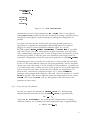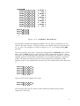
Download ECRC-95-17

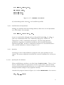
A Tutorial on
Parallelism and
Constraints
in ECLiPSe
Steven Prestwich
ECRC-95-17
technical report ECRC-95-17
A Tutorial on
Parallelism and Constraints
in ECLiPSe
Steven Prestwich
European Computer-Industry
Research Centre GmbH
(Forschungszentrum)
Arabellastrasse 17
D-81925 Munich
Germany
Tel. +49 89 9 26 99-0
Fax. +49 89 9 26 99-170
Tlx. 52 69 10
I
c European Computer-Industry Research Centre, 1995
Although every effort has been taken to ensure the accuracy of this report,
neither the authors nor the European Computer-Industry Research Centre
GmbH make any warranty, express or implied, or assume any legal liability for
either the contents or use to which the contents may be put, including any
derived works. Permission to copy this report in whole or in part is freely
given for non-profit educational and research purposes on condition that such
copies include the following:
1. a statement that the contents are the intellectual property of the
European Computer-Industry Research Centre GmbH
2. this notice
3. an acknowledgement of the authors and individual contributors to
this work
Copying, reproducing or republishing this report by any means, whether
electronic or mechanical, for any other purposes requires the express written
permission of the European Computer-Industry Research Centre GmbH. Any
registered trademarks used in this work are the property of their respective
owners.
For more
information
please
contact :
[email protected]
II
Abstract
This is a tutorial for the working programmer on the ECLi PSe parallel constraint
logic programming language. It assumes previous experience of ECLiPSe , or at
least some version of Prolog, and introduces the parallelism and constraints
features. For further details on these and other features see the User Manual
and Extensions User Manual.
III
Contents
1 Introduction
1.1
How to read this tutorial
3
: : : : : : : : : : : : : : : : : : : : : : :
2 OR-Parallelism
2.1
2.2
2.3
2.4
How to use it : : : : : : : : : : : : : : :
How it works : : : : : : : : : : : : : : :
2.2.1 Continuations : : : : : : : : : : :
When to use it : : : : : : : : : : : : : :
2.3.1 Non-deterministic calls : : : : : :
2.3.2 Side effects : : : : : : : : : : : :
2.3.3 The commit operator : : : : : : :
2.3.4 Parallelisation overhead : : : : :
2.3.5 Grain size for all solutions : : : :
2.3.6 Grain size for one solution : : :
2.3.7 Grain size and pruning operators
2.3.8 Grain size and coroutining : : : :
2.3.9 Parallelisation of predicates : : :
2.3.10 Parallelisation of calls : : : : : :
2.3.11 Partial parallelisation : : : : : : :
2.3.12 Parallelisation of disjunctions : :
2.3.13 Speedup : : : : : : : : : : : : : :
Summary : : : : : : : : : : : : : : : : :
4
: : : : : : : : : : : : : :
: : : : : : : : : : : : : :
: : : : : : : : : : : : : :
: : : : : : : : : : : : : :
: : : : : : : : : : : : : :
: : : : : : : : : : : : : :
: : : : : : : : : : : : : :
: : : : : : : : : : : : : :
: : : : : : : : : : : : : :
: : : : : : : : : : : : : :
: : : : : : : : : : : : : :
: : : : : : : : : : : : : :
: : : : : : : : : : : : : :
: : : : : : : : : : : : : :
: : : : : : : : : : : : : :
: : : : : : : : : : : : : :
: : : : : : : : : : : : : :
: : : : : : : : : : : : : :
3 Independent AND-parallelism
3.1
3.2
3.3
3.4
How to use it : : : : : : : : : : :
How it works : : : : : : : : : : :
When to use it : : : : : : : : : :
3.3.1 Non-logical calls : : : : :
3.3.2 Non-terminating calls : : :
3.3.3 Shared variables : : : : :
3.3.4 Parallelisation overhead :
3.3.5 Conditional parallelisation
3.3.6 Speedup : : : : : : : : : :
Summary : : : : : : : : : : : : :
4
5
5
6
6
6
7
9
10
11
11
12
13
15
16
17
17
18
20
: : : : : : : : : : : : : : : : : :
: : : : : : : : : : : : : : : : : :
: : : : : : : : : : : : : : : : : :
: : : : : : : : : : : : : : : : : :
: : : : : : : : : : : : : : : : : :
: : : : : : : : : : : : : : : : : :
: : : : : : : : : : : : : : : : : :
: : : : : : : : : : : : : : : : : :
: : : : : : : : : : : : : : : : : :
: : : : : : : : : : : : : : : : : :
4 Finite Domain constraint handling
4.1
4.2
3
Description of the 8-queens problem
Logic programming methods : : : : :
4.2.1 Generate-and-test : : : : : : :
4.2.2 Test-and-generate : : : : : : :
4.2.3 Standard backtracking : : : :
20
20
21
21
22
23
24
25
25
26
27
: : : : : : : : : : : : : : : :
: : : : : : : : : : : : : : : :
: : : : : : : : : : : : : : : :
: : : : : : : : : : : : : : : :
: : : : : : : : : : : : : : : :
27
27
28
28
29
1
4.3
4.4
4.5
4.6
4.2.4 Forward checking : : : : : : :
Constraint logic programming methods
4.3.1 Forward checking : : : : : : :
4.3.2 Generalised forward checking :
4.3.3 The first-fail principle : : : : :
4.3.4 Maximising propagation : : : :
Non-logical calls : : : : : : : : : : : :
Parallelism : : : : : : : : : : : : : : : :
Summary : : : : : : : : : : : : : : : :
: : : : : : : : : : : : : : :
: : : : : : : : : : : : : : :
: : : : : : : : : : : : : : :
: : : : : : : : : : : : : : :
: : : : : : : : : : : : : : :
: : : : : : : : : : : : : : :
: : : : : : : : : : : : : : :
: : : : : : : : : : : : : : :
: : : : : : : : : : : : : : :
A Calculating parallel speedup
A.1 The obvious definition : : : : : :
A.2 A better definition : : : : : : : :
A.2.1 A note on calculation : :
A.2.2 Other applications : : : :
A.2.3 Quasi standard deviation :
A.3 Speedup curves : : : : : : : : : :
30
30
30
30
31
32
33
33
34
35
: : : : : : : : : : : : : : : : : :
: : : : : : : : : : : : : : : : : :
: : : : : : : : : : : : : : : : : :
: : : : : : : : : : : : : : : : : :
: : : : : : : : : : : : : : : : : :
: : : : : : : : : : : : : : : : : :
35
36
36
36
37
37
2
1 Introduction
Logic programming has the well-known advantages of ease of programming
(because of its high level of abstraction) and clarity (because of its logical
semantics). The main drawback is its slow execution times compared to those
of conventional, imperative languages. In recent years, research has produced
various extensions which make such systems competitive.
ECLi PSe , the ECRC Prolog platform, is a logic programming system with several
extensions. Two of these extensions are targeted at problems with large search
spaces; these are constraint handling and parallelism . Constraints are used to
prune search spaces, whereas parallelism exploits parallel or distributed
machines to search large spaces more quickly. These complementary
techniques can be used separately or combined to obtain clear, concise and
efficient programs. These extensions originated in other ECRC systems:
constraint handling came from CHIP and the parallelism from ElipSys, both
with some changes.
This tutorial is adapted and extended from a similar tutorial for ElipSys [5]. It
provides some general principles on how to make the best use of parallelism
and constraints. It is intended as an introduction for the working programmer,
and does not contain details of all the built-in predicates available. These
details can be found in the Manuals.
1.1
How to read this tutorial
If you are just interested in OR-parallelism then go directly to Chapter 2, which
is self-contained. This is the most important form of parallelism in ECLi PSe . If
you are just interested in AND-parallelism then read Chapter 2 followed by
Chapter 3, because 2 contains information necessary to understand 3. When
you are ready to test OR- or AND- parallel programs for performance,
Appendix A describes how to handle timing variations when calculating parallel
speedups, and includes a note on speedup curves. If you are just interested in
constraints then jump to Chapter 4 which is self contained, except for Section
4.5 which links the ideas of constraints and parallelism. If you are interested in
all aspects of parallelism and constraints, then just read the chapters in order.
3
2 OR-Parallelism
Many programming tasks can be naturally split into two or more independent
subtasks. If these subtasks can be executed in parallel on different processors,
much greater speeds can be achieved. Parallel hardware is becoming cheaper
and more widely available, but programming these machines can be much
more difficult than programming sequential machines. Using conventional,
imperative languages may involve the programmer in a great deal of low-level
detail such as communication, load balancing etc. This difficulty in exploiting
the hardware is sometimes called the programming bottleneck . ECLi PSe avoids
this bottleneck. It exploits parallel hardware in an almost transparent way, with
the system taking most of the low-level decisions. However, there are still
certain programming decisions to be made regarding parallelism, and this
tutorial gives some practical hints on how to make these decisions. In the
future even greater transparency will be achieved as analysis and
transformation tools are developed.
2.1
How to use it
First, we must tell ECLiPSe how many processors to allocate for the program.
One way to do this is to specify the number of workers when parallel
ECLi PSe is called. For example
peclipse -w 3
calls parallel ECLi PSe with 3 workers. If no number of workers is specified,
ECLi PSe will simply run sequentially with the default of 1 worker. Other ways
of changing the number of workers are described in [1, 2].
For the purpose of this tutorial we shall assume that a worker and a
processor are the same thing, though there is a subtle difference: it is possible
to specify a greater number of workers than there are processors, in which case
ECLi PSe will simulate extra processors. Simulated parallelism is useful for some
search algorithms, as it causes the program to search in a more “breadth-first”
way. However, it does add an overhead and uses more memory, so it should
only be used when necessary.
Note:
As a simple example, here is part of a program:
p(X) :- p1(X).
p(X) :- p2(X).
4
In a standard Prolog execution, a call to p will first enumerate the answers to
p1, then on backtracking those of p2.
We can tell ECLi PSe to try p1 and p2 in parallel instead of by backtracking
simply by inserting a declaration
:- parallel p/1.
p(X) :- p1(X).
p(X) :- p2(X).
The set of answers for p will still be the same in parallel as in the backtracking
computation, though possibly in a different order.
For convenience, some built-in predicates have been pre-defined as OR-parallel
in the library par_util. For example par_member/2 is an OR-parallel version
of the list membership predicate member/2. Before defining new parallel
predicates it is worth checking whether they already exist in the library.
2.2
How it works
The computation of p splits into two (or more if there are more p clauses)
parallel computations which may be executed on separate workers if any are
available, and if ECLi PSe decides to do so — these decisions are made
automatically by the ECLi PSe task scheduler, and need not concern the
programmer.
2.2.1
Continuations
Not only will p1 and p2 be computed in parallel, but also any calls occurring
after p in the computation. This part of the computation is called the
continuation of the p call.
For example, if p is called from another predicate:
q(X,Y) :- r(X), s(X), t(Y).
s(X) :- u(X), p(X), v(X).
:- parallel p/1.
p(X) :- p1(X).
p(X) :- p2(X).
5
then p(X) has two alternative continuations in a computation of :- q(f(A),Y):
p1(f(A)), v(f(A)), t(Y)
p2(f(A)), v(f(A)), t(Y)
and it is these processes which will be assigned to separate workers. The idea
of a continuation plays a large part in deciding where to use OR-parallelism.
2.3
When to use it
When should we declare predicates as OR-parallel? It may appear that all
predicates with more than one clause should be parallel, but this is wrong. In
this section we discuss why it is wrong, indicate possible pitfalls, and consider
the effects of OR-parallelism on execution times.
2.3.1
Non-deterministic calls
Since a parallel declaration tells the system that the clauses of the predicate
should be tried in parallel, clearly only predicates with more than one clause
are candidates. Furthermore, deterministic predicates should not be parallel,
that is those whose calls only ever match one clause at runtime. For example,
the standard list append predicate:
append([],A,A).
append([A|B],C,[A|D]) :- append(B,C,D).
is commonly called with its first argument bound to concatenate two lists. Only
one clause will match any such call, and there is no point in making append
parallel. If append is called in other modes, for example with only its third
argument bound, then it is nondeterministic and may be worth parallelising.
2.3.2
Side effects
Only predicates whose solution order is unimportant should be parallel. An
example of a predicate whose solution order may be important is
p :- generate1(X), write(X).
p :- generate2(X), write(X).
p :- generate3(X), write(X).
6
q :- ... p(X) ...
:- parallel p/1.
p(X) :- guard1(X), !.
p(X) :- guard2(X), !.
p(X) :- guard3(X), !.
Figure 2.3.1:
A simple predicate with commit
where generate{1,2,3} generate values for X non-deterministically. If p is
parallelised then the order of write’s may change. In fact any side effects in
the continuation of a parallel call may occur in a different order. This may or
may not be important, only the programmer can decide.
Even if solution order is unimportant, it is recommended that any predicates
with side effects such as read, write or setval are only used in sequential
parts of the program, otherwise the performance of the system may be
degraded. The OR-parallelism of ECLi PSe is really designed to be used for pure
search. If parallel solutions are to be collected then there are built-in predicates
like findall which should be used.
2.3.3
The commit operator
When the cut ! is used in parallel predicates, it has a slightly different meaning
than in normal (sequential) predicates. When used in parallel in ECLi PSe it is
called the commit operator. Its meaning can be explained using examples.
First consider Figure 2.3.1. The “guards” execute in parallel, and as soon as one
finds a solution the commit operator aborts the other two guards. Only the
continuation of the successful guard survives.
This simple example can be written in another way using the once
meta-predicate, as in Figure 2.3.2. This is a matter of preferred style.
In the more general case there may be calls after the commits, as in Figure
2.3.3. The commit has exactly the same effect as before, with the body calls at
the start of the parallel continuations. By the way, this example cannot be
rewritten using once without a little program restructuring, because of the body
calls.
Some predicates may have an empty guard, corresponding to (for example) the
“else” in Pascal. An example is shown in Figure 2.3.4 The meaning of this
predicate is “if guard1 then body1, else if guard2 then body2, else body3”. This
must not be parallelised simply by adding a declaration, because the empty
7
q :- ... once(p(X)) ...
:- parallel p/1.
p(X) :- guard1(X).
p(X) :- guard2(X).
p(X) :- guard3(X).
Figure 2.3.2:
Replacing commits by \once" in a simple parallel predicate
q :- ... p(X) ...
:- parallel p/1.
p(X) :- guard1(X), !, body1(X).
p(X) :- guard2(X), !, body2(X).
p(X) :- guard3(X), !, body3(X).
Figure 2.3.3:
A less simple predicate with commit
p(X) :- guard1(X), !, body1(X).
p(X) :- guard2(X), !, body2(X).
p(X) :body3(X).
Figure 2.3.4:
A typical sequential predicate with empty guard
8
p(X) :guard1(X), !, body1(X).
p(X) :guard2(X), !, body2(X).
p(X) :- not guard1(X), not guard2(X), !, body3(X).
Figure 2.3.5:
Handling empty guards when parallelising
p(X) :- guards(X,N), !, bodies1_and_2(N,X).
p(X) :- body3(X).
:- parallel guards/2.
guards(X,1) :- guard1(X).
guards(X,2) :- guard2(X).
bodies_1_and_2(1,X) :- body1(X).
bodies_1_and_2(2,X) :- body2(X).
Figure 2.3.6:
Another way of handling empty guards when parallelising
guard may change the meaning of the program when executed in parallel. The
reason is that if we make p parallel then we may get body3 succeeding
followed by (guard1, !, body1) or (guard2, !, body2) giving more
solutions for p than in backtracking mode.
It is safer to use commits in each of the p clauses and to introduce a new
guard, as in Figure 2.3.5. This is now safe, but at the expense of introducing
extra work (the negated guards in the third clause). A safe and efficient
method, though slightly more complicated, is shown in Figure 2.3.6 where we
split the definition of p into parallel and sequential parts.
2.3.4
Parallelisation overhead
Even if a program is safely parallelised it may not be worthwhile making a
predicate parallel. For example, in a Quick Sort program there is typically a
partition predicate as shown in Figure 2.3.7. Although for most calls to
partition both clauses 2 and 3 will match, one of them will fail almost
partition([],_,[],[]).
partition([H|T],D,[H|S],B) :- H<D, partition(T,D,S,B).
partition([H|T],D,S,[H|B]) :- H>=D, partition(T,D,S,B).
Figure 2.3.7:
Quick Sort partitioning predicate
9
process_value :value(X),
process(X).
value(1).
value(2).
:
value(n).
Figure 2.3.8:
Grain size estimation
immediately because of the comparison H<D or H>=D. There is no point in
making partition parallel because the overhead of starting a parallel process
will greatly outweigh the small advantage of making the comparisons in
parallel.
To express the fact that the overhead of spawning parallel processes is
equivalent to a significant computation (depending upon the hardware,
perhaps as much as several hundred resolution steps) we say that
. The
of a parallel
ECLi PSe supports
task refers to the cost of its computation, roughly equivalent to its cpu time.
Only computations with grain size at least as large as this overhead are worth
executing in parallel, in fact the grain size should be much larger than the
.
overhead. Computations which are not coarse-grained are called
coarse-grained parallelism
grain size
ne-grained
Estimating grain sizes is usually not as obvious as in the Quick Sort example.
In fact it is the most difficult aspect of using OR-parallelism, and we therefore
spend some time discussing it. In the context of OR-parallelism, a parallel task
is a continuation, and so when we refer to the grain size of a parallel predicate
call we mean the time taken to execute that call plus its continuation. To
illustrate this, consider the program in Figure 2.3.8, where process(X)
performs some computation using the value of X. Now the question is, should
value be parallel? The answer depends upon the computations of the various
process calls since the value calls are fine-grained. We now discuss this
question in some detail.
2.3.5
Grain size for all solutions
Say that we require all solutions of process_value. In a backtracking
computation the total time to execute process_value is approximately
t1 + : : : + tn
where ti = time(process(i)). In an OR-parallel computation (assuming
sufficient workers are available) the total computation time is approximately
k + maximum(t1 : : : tn)
10
where k is the overhead of starting a parallel process, which is machine and
implementation dependent. As can be seen from the formulae, if process has
no expensive calls then k becomes significant, and the backtracking
computation is faster;
one expensive call then the sequential and parallel cases will take about
the same time;
two or more expensive calls then k is insignificant and the parallel
computation is faster.
The programmer must try to ensure that at least two continuations have
significant cost.
2.3.6
Grain size for one solution
Say that we only require process_value to succeed once. In a backtracking
computation the time will be
t1 + : : : + ts
where s is the number of the first succeeding process(s). In a parallel
computation the time will be
k + minimum(t1 : : :tn)
Now the parallel computation is only cheaper if there are
of i s for which process(i) is expensive.
2.3.7
one or more values
Grain size and pruning operators
Pruning operators such as the commit may affect estimates of the grain size of
a continuation. Consider the program in Figure 2.3.9. Here n processes will be
spawned with continuations
process1(1), !, process2(1).
:
process1(n), !, process2(n).
As soon as process1 on one worker succeeds, all the other workers will
abandon their computations. Hence the actual grain size of any continuation of
an OR-parallel call is no greater than that of the cheapest process before
pruning occurs. Of course, it may be smaller than this if failure occurs before
the pruning operator is reached.
11
one_process_value :value(X),
process1(X),
!,
process2(X).
:- parallel value/1.
value(1).
value(2).
:
value(n).
Figure 2.3.9:
Grain size estimation and an obvious commit
p1 :- p2, !.
p2 :- process_value, p3.
process_value :value(X),
process(X),
Figure 2.3.10:
Grain size estimation and a less obvious commit
In fact, we must consider the effects of commits in any predicate which calls a
parallel predicate, even indirectly. For example, see the program in Figure
2.3.10. Since p1 contains a commit which prunes p2, and p2 calls value
(indirectly), we only need to estimate the grain size of the continuation up to
the commit, that is the grain size of
process(X), p3
The same holds for any pruning operator, including once/1, not/1 and ->
(if-then-else) because these contain implicit commits. When we talk about a
continuation for an OR-parallel call in future, we shall mean the continuation
up to the first pruning operator.
2.3.8
Grain size and coroutining
When estimating the grain size of a continuation, we must take into account
any suspended calls which may be woken during the computation. For
example, consider the program in Figure 2.3.11. When deciding whether to
parallelise process we estimate the grain sizes of
12
delay expensive_process(A) if nonground(A).
p :- expensive_process(X), process, X=0.
process :- cheap_process1.
process :- cheap_process2.
Figure 2.3.11:
Grain size estimation and coroutining, rst example
delay expensive_process(A) if nonground(A).
p :- process, expensive_process(X), !, X=0.
process :- cheap_process1.
process :- cheap_process2.
Figure 2.3.12:
Grain size estimation and coroutining, second example
cheap_process1, X=0
cheap_process2, X=0
These appear to be cheap, but at runtime X=0 wakes expensive_process and
so it is effectively expensive.
On the other hand, given the program in Figure 2.3.12, it appears that process
has two expensive continuations
cheap_process1, expensive_process(X)
cheap_process2, expensive_process(X)
before the commit occurs, but this is deceptive because expensive_process is
not woken until after the commit.
2.3.9
Parallelisation of predicates
So far we have discussed when it is worthwhile making a call OR-parallel.
However, in ECLi PSe we parallelise calls indirectly by deciding whether to
declare a predicate parallel or not. To do this, the programmer must consider
the most important calls to the predicate, that is the calls which have greatest
effect on the total computation. If they would be faster in parallel then the
predicate should be declared as parallel. For some predicates this may be easy
to see but others may be called in many different ways.
13
berghel :word(A1,A2,A3,A4,A5),
word(A1,B1,C1,D1,E1),
word(B1,B2,B3,B4,B5),
word(A2,B2,C2,D2,E2),
word(C1,C2,C3,C4,C5),
word(A3,B3,C3,D3,E3),
word(D1,D2,D3,D4,D5),
word(A4,B4,C4,D4,E4),
word(E1,E2,E3,E4,E5),
word(A5,B5,C5,D5,E5).
%
%
%
%
%
%
%
%
%
%
column
row
column
row
column
row
column
row
column
row
1
1
2
2
3
3
4
4
5
5
word(a,a,r,o,n).
word(a,b,a,s,e).
word(a,b,b,a,s).
:
Figure 2.3.13:
Sequential Berghel program
For example consider the Berghel problem. We are given a dictionary of 134
words each with 5 letters. We must choose 10 of them which can be placed in
a 5 5 grid. The program is shown in Figure 2.3.13. Is it worth making word
parallel?
We must consider grain sizes. During the computation of berghel there will be
many calls to word, with all, some or none of the arguments bound to a letter.
The grain size will depend partly upon how many letters are bound. It will also
depend upon the bound letters themselves, for example binding an argument
to a z will almost certainly prune the search more than binding it to an a.
Another factor is the continuation of each call. The continuation of the fifth call
is
word(A3,B3,C3,D3,E3),
word(D1,D2,D3,D4,D5),
word(A4,B4,C4,D4,E4),
word(E1,E2,E3,E4,E5),
word(A5,B5,C5,D5,E5)
whereas that of the eighth call is only
word(E1,E2,E3,E4,E5),
word(A5,B5,C5,D5,E5)
The cheaper calls may be slower when called in parallel and the more
expensive calls faster.
14
berghel :parword(A1,A2,A3,A4,A5),
parword(A1,B1,C1,D1,E1),
word(B1,B2,B3,B4,B5),
word(A2,B2,C2,D2,E2),
word(C1,C2,C3,C4,C5),
word(A3,B3,C3,D3,E3),
word(D1,D2,D3,D4,D5),
word(A4,B4,C4,D4,E4),
word(E1,E2,E3,E4,E5),
word(A5,B5,C5,D5,E5).
:- parallel parword/5.
parword(a,a,r,o,n).
parword(a,b,a,s,e).
parword(a,b,b,a,s).
:
Figure 2.3.14:
Parallelising selected calls
The result of parallelising word is the net result of all these effects, which can
best be estimated by experimentation (trace visualisation and profiling tools,
when available, can help greatly).
2.3.10 Parallelisation of calls
We can make more selective use of OR-parallelism by parallelising only some
calls. In the Berghel example, if we keep word sequential and add a new
parallel version as in Figure 2.3.14 then we can experiment by replacing
various calls to word by calls to parword. The question is, which calls should
be parallel?
Running this program on a SUN SPARCstation 10 model 51 with 4 CPU’s it turns
out that the best result (a speedup of about 3:3) is obtained when all the calls
are parallel — in other words, simply declaring word parallel. However, this
may not be true for all machines and all numbers of workers. This example
behaves differently in experiments with ElipSys on a Sequent Symmetry with 10
workers, and we conjecture that similar effects will be observed in ECLi PSe with
more workers, or on parallel machines with faster cpu’s. With all word calls
parallel we get a speedup of 6:7, but if we only parallelise the first 2 calls as in
Figure 2.3.14 we obtain an almost linear speedup of 9:7. So in some cases it is
worth a little experimentation and programming effort to selectively parallelise
calls.
15
process_value :value(X),
process(X).
value(1).
value(2).
value(3).
value(4).
%
%
%
%
leads
leads
leads
leads
to
to
to
to
cheap process
expensive process
cheap process
expensive process
Figure 2.3.15:
A program worth partially parallelising
process_value :value(X),
process(X).
value(X) :- value13(X).
value(X) :- value24(X).
value13(1).
value13(3).
:- parallel value24/1.
value24(2).
value24(4).
Figure 2.3.16:
Partially parallelised version
In this example we chose between the parallel and sequential versions
according to a static test: the position of the call in a clause. The choice could
also be based on a dynamic property such as instantiation patterns.
2.3.11 Partial parallelisation
Recall that it is worth parallelising a predicate if (for most of its calls) there are
at least two clauses leading to large-grained continuations. If we can predict
which of the clauses may lead to such continuations then we can extract them
from the predicate definition, and avoid spawning small-grained parallel
processes.
For example, consider the sequential program in Figure 2.3.15. If we know
that process(i) is small-grained for i = f1; 3g but large-grained for i = f2; 4g
then it is best to decompose value into backtracking and parallel parts, as
shown in the parallel program of Figure 2.3.16. Then values 1; 3 are handled
16
p(X) :- q(X), new(X), r(X).
:- parallel new/1.
new(X) :- a(X).
new(X) :- b(X).
Figure 2.3.17:
Parallelised disjunction
by backtracking while values 2; 4 are handled in parallel.
2.3.12 Parallelisation of disjunctions
ECLi PSe (in common with most Prolog dialects) allows the use of disjunctions
in a clause body. For example,
p(X) :- q(X), (a(X); b(X)), r(X).
It may be worthwhile calling a and b in OR-parallel mode if a, r and b, r
(plus any continuation of p) have sufficiently large grain. The use of
disjunction is really a notational convenience, and may hide potential
parallelism. Of course it would be possible to add a parallel disjunction
operator to ECLi PSe , but this is unnecessary because we can instead make a
new, parallel definition as shown in Figure 2.3.17.
2.3.13 Speedup
Assuming we have OR-parallelised a program well, what speedup can we
expect? The answer depends on whether we want all solutions to a call or just
one.
2.3.13.1 Speedup for all solutions
When parallelising a predicate, we often hope for linear speedup . That is, if we
have N workers then we want queries to run N times faster. Because of the
overhead of spawning parallel processes we usually obtain sublinear speedup,
though with fine tuning we may approach linearity.
Consider the program shown in Figure 2.3.18 where ascending(X) has answers
X=1, X=2, ... X=1000
17
:- worker(2).
p(X) :- ascending(X),
p(X) :- descending(X).
Figure 2.3.18:
Ascending-descending example
descending(X) has answers
X=1000, ... X=2, X=1
and both ascending(X) and descending(X) take time t to find each successive
answer (where t is much greater than the parallel overhead k ).
With 2 workers the time taken to find all solutions for p is 2000t with p
sequential, but 1000t + k with p parallel: almost linear speedup.
2.3.13.2 Speedup for one solution
However, when using a predicate to find one solution, we generally find little
relationship between execution times in backtracking and OR-parallel modes,
except when averaged over many queries. This is because solutions may not
be distributed evenly over the search space.
The time to find one solution for the query p(X), X=1000 is 1000t with p
sequential (999 failing calls followed by 1 succeeding call to ascending), but
t + k with p parallel (an immediately succeeding call to descending). This is a
speedup of almost 1000 using only 2 workers: very superlinear speedup.
On the other hand, the time to find one solution for the query p(X), X=1 is t
with p sequential and t + k with p parallel: no speedup at all.
This shows that for single-solution queries the difference between superlinear
speedup and no speedup may depend only on the query.
2.4
Summary
The best use will be made of OR-parallelism if the programmer keeps it in
mind from the start. However, a program written for sequential ECLi PSe can be
parallelised using the principles outlined in this section. Here is a summary of
the principles.
18
Look for predicates which are worth declaring as OR-parallel. When
deciding this, all runtime calls to the predicate must be considered. If all,
or almost all, calls to a predicate would be faster in OR-parallel, and if it
is always safe to do so, then it is worth declaring the predicate as parallel.
If it is sometimes worth calling in OR-parallel and sometimes not (but
always safe), then a useful technique is to make a parallel and a
sequential definition of the predicate and use them where appropriate.
A call is unsafe in OR-parallel if it has side effects in any of its
continuations, or if it has commits in some but not all of its clauses.
A call is (probably) faster in OR-parallel if it has at least two expensive
continuations. A continuation should only be considered up to the first
commit or other pruning operator which affects it, and taking into
account any suspended calls.
To further refine a program, look for parallel predicates with some
clauses which do not have expensive continuations, then isolate the
useful clauses in a new parallel definition. Also look for disjunctions in
clause bodies which may hide parallelism, and replace these by calls to
new parallel predicates.
The once operator is sometimes stylistically preferable to the use of
commits in parallel predicates.
However, these principles do not guarantee the best speedups. In [6, 7] we
described various ways in which (for example) two parallel declarations could
combine to give a poor speedup, even though each alone gave a good
speedup. We also showed that improving a parallel predicate may have a
good, bad or no effect on overall speedup. Effects like these make tuning a
parallel program rather harder than tuning a sequential one. Note that they are
not ECLi PSe bugs and will occur in many parallel programs. They may be more
obvious in ECLi PSe since parallelisation of logic programs is very easy. The
significance of these effects is that they make it hard to recommend a good
general strategy. Probably the best approach is common sense based on
knowledge of the program, plus the use of available programming tools.
ECLi PSe will soon have at least one trace visualisation tool to aid parallelisation.
19
3 Independent AND-parallelism
As well as OR-parallelism ECLi PSe supports independent AND-parallelism,
which is used in quite different circumstances. AND-parallelism replaces the
left-to-right computation rule of Prolog by calling two or more calls in parallel
and then collecting the results. Dependent AND-parallelism is rather different,
and is outside the scope of this tutorial.
3.1
How to use it
As with OR-parallelism, we need to tell ECLi PSe how many workers to allocate.
Then we simply replace the usual “,” conjunction operator by a parallel
operator “&”; for example replace
p(X) :- q(X), r(X).
by
p(X) :- q(X) & r(X).
More than two calls can be connected by &.
For convenience there is a built-in predicate which can be used to map one list
to another. This is maplist, and it applies a specified predicate to each
member in AND-parallel. See [1, 2] for details.
3.2
How it works
As an example (which is not to be taken as a useful candidate for
AND-parallelism, but only as an illustration), consider the program in Figure
3.2.1. In standard Prolog, given a query :-p(X), q is first solved to return the
answer X=a then r is called, fails, and backtracking occurs. The next solution
to q is X=b and again r fails. For the next solution X=c, r succeeds. On
backtracking no more solutions are found.
Now if we call q and r in AND-parallel:
p(X) :- q(X) & r(X).
20
p(X) :- q(X), r(X).
q(a).
q(b).
q(c).
r(c).
r(d).
r(e).
Figure 3.2.1:
Simple AND-parallelism example
what happens instead is that the solutions {X=a, X=b, X=c} of q and
{X=c, X=d, X=e} of r are collected independently using different workers,
and then the results are merged to give the consistent set {X=c}. This is clearly
a rather different strategy for executing a program, and in this section we
discuss when it is better than the usual strategy.
As with OR-parallelism, it is not always true that different workers will be
assigned to AND-parallel calls, depending upon runtime availability. This need
not concern the programmer.
3.3
When to use it
When should AND-parallelism be used? It may seem at first glance that it will
always be faster than the usual sequential strategy, but as often with parallelism
this intuition is wrong. In this section we discuss when to apply
AND-parallelism.
3.3.1
Non-logical calls
It is sometimes incorrect to use AND-parallelism because of side effects and
other non-logical Prolog features. For example
p(X) :- generate(X), test(X).
test(X) :- X\==badterm, rest_of_test(X).
Here generate(X) binds X to some term, and test(X) performs some test on
X, including the non-logical test X\==badterm. Say that the answers to
generate(X) are
{X=goodterm1, X=goodterm2, X=badterm}
and the terms permitted by rest_of_test(X) are
21
{X=goodterm1, X=badterm}
Then p has only one answer {X=goodterm1}
However, if we use AND-parallelism:
p(X) :- generate(X) & test(X).
then test(X) is first called with X unbound, and has answers
{X=goodterm1, X=badterm}
Merging this with the answers for generate(X) we get more answers:
{X=goodterm1, X=badterm}
which is incorrect. Examples can also be found where a program fails instead
of generating solutions.
3.3.2
Non-terminating calls
AND-parallel calls must terminate when called in any order. For example, given
p(L1,L2) :append([LeftHead|LeftTail],Right,L1),
append(Right,[LeftHead|LeftTail],L2).
where append is the usual list append predicate. This program with a query
:-p([1,2,3],L2)
would give answers
{L2=[2,3,1], L2=[3,1,2], L2=[1,2,3]}
But if we use AND-parallelism:
p(L1,L2) :append([LeftHead|LeftTail],Right,L1) &
append(Right,[LeftHead|LeftTail],L2).
22
then the call
append(Right,[LeftHead|LeftTail],L2)
will not terminate because Right is unbound.
3.3.3
Shared variables
Even if the calls can safely be executed in any order, it is not necessarily worth
calling them in AND-parallel. If the answers to one call restrict the answers to
another call, then this pruning effect may give greater speed than finding all
the answers to both calls and then merging the results.
For example consider
p(X) :- compute1(X), compute2(X).
compute2(X) :- cheap_filter(X), compute3(X).
where compute1(X) has the answers
{X=1, X=2, ... X=1000}
and cheap_filter(X) allows the bindings
{X=1000, X=1001, ... X=1999}
Say compute3 performs some expensive computation on X. Now given a query
:-p(X), X is generated by compute1(X) and cheap_filter quickly rejects all
answers except X=1000, so that compute3(X) is only called once. The total
computation time for all solutions is (ignoring the times of cheap_filter for
simplicity)
time(compute1(1)) + : : : + time(compute1(1000))+
time(compute3(1000))
If we use AND-parallelism instead:
p(X) :- compute1(X) & compute2(X).
then compute2(X) is called with X unbound and compute3(X) is called 1000
times for each permitted answer of cheap_filter(X). The total computation
time for all solutions is now (ignoring the parallelism overhead)
maximum(time(compute1(1)) + : : : + time(compute1(1000));
time(compute3(1000)) + : : : + time(compute3(1999)))
23
quicksort([Discriminant|List],Sorted) :partition(List,Discriminant,Smaller,Bigger),
quicksort(Smaller,SortedSmaller),
quicksort(Bigger,SortedBigger),
append(SortedSmaller,[Discriminant|SortedBigger],Sorted).
Figure 3.3.1:
Sequential Quick Sort program
quicksort([Discriminant|List],Sorted) :partition(List,Discriminant,Smaller,Bigger),
quicksort(Smaller,SortedSmaller) &
quicksort(Bigger,SortedBigger),
append(SortedSmaller,[Discriminant|SortedBigger],Sorted).
Figure 3.3.2:
AND-parallel Quick Sort program
Comparing the two times, it can be seen that the parallel time will be slower
than the sequential time if compute3 is more expensive than compute1. By
calling compute1 and compute2 independently we lose the pruning effect of
compute1 on compute2. In fact, in this example cheap_filter should not be
used in independent AND-parallel, but as a constraint or a delayed goal.
3.3.4
Parallelisation overhead
As with OR-parallelism, we must consider the overhead of creating parallel
processes, and only parallelise calls with large grain size. When estimating
grain size for AND-parallelism we do not need to consider continuations, only
the grain size of the calls themselves. Also, because of the way
AND-parallelism is implemented we always estimate grain size for all solutions,
never for one solution.
Consider the Quick Sort program in Figure 3.3.1. For large lists Smaller and
Bigger the grain sizes of the recursive quicksort calls may be large enough to
justify calling them in parallel, as in Figure 3.3.2. Of course, as the input list is
decomposed into smaller and smaller sublists parallelisation becomes less
worthwhile.
In fact Quick Sort is not a good example for ECLiPSe because it is more
concerned with OR-parallelism, and its implementation of AND-parallelism is
not very sophisticated. Since it collects all the results of two AND-parallel
goals, there is an overhead which grows as the sizes of the goal arguments
grow. For the Quick Sort program, coarse-grained goals also have large terms,
and so it is probably never worthwhile using AND-parallelism. We shall use
Quick Sort for purposes of illustration and pretend that this overhead does not
24
quicksort([Discriminant|List],Sorted) :partition(List,Discriminant,Smaller,Bigger),
length(Smaller,SmallerLength),
length(Bigger,BiggerLength),
(SmallerLength>30,
BiggerLength>30 ->
quicksort(Smaller,SortedSmaller) &
quicksort(Bigger,SortedBigger)
; quicksort(Smaller,SortedSmaller),
quicksort(Bigger,SortedBigger)),
append(SortedSmaller,[Discriminant|SortedBigger],Sorted).
Figure 3.3.3:
Conditional AND-parallel Quick Sort program
exist, but the reader should be aware that goals should only be called in
AND-parallel when their arguments are not very large.
3.3.5
Conditional parallelisation
We can make more efficient use of AND-parallelism by introducing runtime
tests. Say that for a given number of workers, lists with length greater than 30
make parallelisation worthwhile, while smaller lists cause fine-grained recursive
calls which do not make it worthwhile. Then we can write the program shown
in Figure 3.3.3.
This can be further refined by making partition calculate the lengths of
Smaller and Bigger as they are constructed, to avoid the expensive calls to
length. In fact, we should be careful of introducing expensive runtime tests.
A point worth noting is that when estimating the grain size of a quicksort(L)
call to set the threshold (30 in this case) we should base the estimate on the
version with the runtime test. The version with the tests will have greater grain
size for a given list length, and so the threshold can be set lower, giving greater
parallelism.
3.3.6
Speedup
It is possible to obtain superlinear speedup with AND-parallelism. For
example, say we have AND-parallel calls (a & b) where b fails immediately.
Then a can be aborted immediately. But if instead we had called (a, b) the
failure of b would not be detected until after a had completed, thus
25
AND-parallelism may cause a large speedup.
1
However, if none of the AND-parallel calls fails then the expected speedup is
linear or sublinear. Unlike OR-parallelism all solutions of AND-parallel calls are
computed, and so there is no difference between one-solution and all-solution
queries. However, when there are not enough workers available AND-parallel
calls will be called using the same worker, as already mentioned. This
execution will be noticeably less efficient than a normal sequential execution.
Therefore AND-parallel calls need to have large grain size so that the overhead
is not significant.
3.4
Summary
A program written for sequential ECLiPSe can be AND-parallelised using the
principles outlined in this chapter. Here is a summary of the principles.
Look for conjunctions of calls which can be called in AND-parallel. First
consider whether they are safe in parallel. It is unsafe to AND-parallelise
calls sharing variables which are used in non-logical calls such as var(X),
X\==Y, setval(X,Y) and read(X). It is also unsafe to AND-parallelise
calls whose results depend upon the order in which they are called.
Next consider whether they will be faster in parallel than in sequence.
Only expensive calls with small arguments are worth calling in parallel.
Also, calls which compete to bind some shared variable will probably be
faster when called sequentially. If a cheap way can be found to estimate
the grain sizes of calls at runtime, then this can be used in a runtime test
to choose between sequential and AND-parallel execution.
As with OR-parallelism, there is no strategy which always leads to the best
speedups. However, a common-sense approach works well in most cases.
1 However, at the time of writing ECLi PSe will
not detect the failure of b in this example; it
may in future versions.
26
4 Finite Domain constraint handling
Constraint handling can speed up search problems by several orders of
magnitude, by pruning the search space in the forward direction (a priori ), in
contrast to backtracking search which prunes in the backward direction (a
posteriori ). Many difficult discrete combinatorial problems can be solved using
constraints which are beyond the reach of pure logic programming systems.
Such problems can of course be solved by special purpose programs written in
imperative languages such as Fortran, but this involves a great deal of work
and results in large programs which are hard to modify or extend. CLP
programs are much smaller, clearer and easier to experiment with. ECLi PSe has
incorporated a number of constraint handling facilities for this purpose. For an
overview on constraint logic programming see [4], from which some of the
examples below have been adapted.
We shall illustrate how to use the finite domains in ECLiPSe with a single
example: the overused but useful 8-queens problem.
4.1
Description of the 8-queens problem
Consider a typical combinatorial problem. We have several variables each of
which can take values from some finite domain. Choosing a value for any
variable imposes restrictions on the other variables. The problem is to find a
consistent set of values for all the variables.
For example, consider the ubiquitous 8-queens problem. We have a chess
board, 8 8 squares, and 8 queens, and we wish (for some reason) to place all
these queens on the board so that no queen attacks another. It is well known
that there are 92 ways of doing this.
Placing any queen on the board typically imposes new restrictions by attacking
several new squares: along the vertical, horizontal and two diagonal lines. It is
possible to imagine many strategies for placing the queens on the board. We
now discuss some of these and their expression in ECLi PSe .
4.2
Logic programming methods
Before describing how to use constraints, we give several versions without
constraints. These will help to illustrate the later versions and to contrast the
27
eight_queens(Columns) :Columns = [_,_,_,_,_,_,_,_],
Numbers = [1,2,3,4,5,6,7,8],
permutation(Columns,Numbers),
safe(Columns).
safe([]).
safe([Column|Columns]) :noattack(Column,Columns,1),
safe(Columns).
noattack(Column,[],Offset).
noattack(Column,[Number|Numbers],Offset) :Column =\= Number - Offset,
Column =\= Number + Offset,
NewOffset is Offset + 1,
noattack(Column,Numbers,NewOffset).
Figure 4.2.1:
8-queens by generate-and-test
two approaches.
4.2.1
Generate-and-test
The most obvious formulation is a purely generate-and-test program which
places all the queens on the board and then checks for consistency (no queen
attacks another). This is shown in Figure 4.2.1: permutation is a library
predicate which generates every possible permutation of the list
[1,2,3,4,5,6,7,8] non-deterministically, and safe checks for consistency.
The first number in the list denotes the row of the first queen (in column 1),
the second number the row of the second queen (in column 2) and so on.
This is arguably the most natural program, but extremely inefficient.
4.2.2
Test-and-generate
With a small change, the generate-and-test program can be made quite good.
We simply reverse the calls in the eight_queens clause and use coroutining to
suspend the checks until they can be made. This is shown in Figure 4.2.2.
Now all the checks are set up initially and suspended, and then the queens are
placed one by one. Each time a queen is placed the relevant checks are woken
immediately, thus interleaving placements with checks. This is closer to the
way in which a human would proceed.
28
eight_queens(Columns) :Columns = [_,_,_,_,_,_,_,_],
Numbers = [1,2,3,4,5,6,7,8],
safe(Columns),
permutation(Columns,Numbers).
noattack(Column,[],Offset).
noattack(Column,[Number|Numbers],Offset) :check(Column,Number,Offset),
NewOffset is Offset + 1,
noattack(Column,Numbers,NewOffset).
delay check(A,B,C) if nonground(A).
delay check(A,B,C) if nonground(B).
delay check(A,B,C) if nonground(C).
check(Column,Number,Offset) :Column =\= Number - Offset,
Column =\= Number + Offset,
Figure 4.2.2:
4.2.3
8-queens by test-and-generate
Standard backtracking
The next most obvious formulation is to explicitly interleave the consistency
checks with the placing of the queens. A typical such program is shown in
Figure 4.2.3.
This is a fairly clear program, and more efficient than the previous program
because it has no coroutining overhead. But it is not the best available; in fact
if we increase the number of queens (and the size of the board) it becomes
hopelessly inefficient.
eight_queens(Columns) :solve(Columns,[],[1,2,3,4,5,6,7,8]).
solve([],_,[]).
solve([Column|Columns],Placed,Number) :delete(Column,Number,Number1),
noattack(Column,Placed,1),
solve(Columns,[Column|Placed],Number1).
Figure 4.2.3:
8-queens by backtracking
29
4.2.4
Forward checking
The strategy can be improved by a technique called forward checking . Each
time we place a queen, we immediately remove all attacked squares from the
domains of the remaining unplaced queens. The trick is that if any domain
becomes empty we can immediately backtrack, whereas in the previous
program we would not backtrack until we tried to place the later queen. All
the useless steps in between are thus eliminated.
A Prolog program using forward checking can be written, but we shall not
show it here because it is rather long. It maintains a list of possible squares for
each queen, and every time a queen is placed these lists must be reduced.
The program is indeed more efficient for a large number (larger than about 12)
of queens, but for fewer queens it is less efficient because of the overhead of
explicitly handling the variable domains. It is also considerably less clear than
the previous program.
4.3
Constraint logic programming methods
We now come to constraint handling. We shall compare and contrast these
methods with the Prolog methods described above.
4.3.1
Forward checking
We can very easily write a forward checking program for 8-queens, as in Figure
4.3.1. The ## built-in predicate is the ECLi PSe disequality constraint.
This program looks similar to the standard backtracking program, but even
simpler because the variable domains are not explicitly manipulated. Instead
they are an implicit property of the domain variables, set up by the call
Columns :: 1 .. 8. The program works in much the same way as the Prolog
forward checking program, but is more efficient.
4.3.2
Generalised forward checking
We can also write a constraints analogue to the test-and-generate program,
which gives more sophisticated forward checking. When we place a queen,
not only can we check for empty domains but also for singleton domains.
Placing a queen may reduce a remaining queen’s domain to one value, and we
can immediately place that queen and do further forward checking. This is
called generalised forward checking .
30
eight_queens(Columns) :Columns=[_,_,_,_,_,_,_,_],
Columns :: 1 .. 8,
solve(Columns).
solve([Column]) :indomain(Column).
solve([Column1,Column2|Columns]) :indomain(Column1),
noattack(Column1,[Column2|Columns],1),
solve([Column2|Columns]).
noattack(Column,[],Offset).
noattack(Column1,[Column2|Columns],Offset) :Column1 ## Column2,
Column1 ## Column2 + Offset,
Column1 ## Column2 - Offset,
NewOffset is Offset+1,
noattack(Column1,Columns,NewOffset).
Figure 4.3.1:
8-queens by forward checking
This will be better than the previous program. We should do as much
propagation as possible at each step, because a propagation step is
deterministic whereas placing a queen is non-deterministic.
The forward checking program provides no opportunity to do this, because
when placing each queen not all the constraints have been called yet. We need
a different formulation, as in Figure 4.3.2. This is similar to the
test-and-generate program, though much faster because of forward checking. It
sets up all the relevant constraints and only then does it begin to place the
queens. Note that the placequeens call could actually be replaced by a call to
the equivalent library predicate labeling. However, we will modify
placequeens below, so it is useful to show it here.
4.3.3
The first-fail principle
Forward checking can be improved by the rst-fail principle . In this technique,
we do not simply place the queens in the arbitrary order 1,2,3... but instead
choose a more intelligent order.
The first-fail principle is a well-known principle in Operations Research, which
states that given a set of possible choices we should choose the most
deterministic one first. That is, if we have to choose between placing the
seventh queen which has 3 possible positions, and the sixth queen which has 5
31
eight_queens(Columns) :Columns=[_,_,_,_,_,_,_,_],
Columns :: 1 .. 8,
safe(Columns),
placequeens(Columns).
safe([]).
safe([Column|Columns]) :noattack(Column,Columns,1),
safe(Columns).
placequeens([]).
placequeens([Column|Columns]) :indomain(Column),
placequeens(Columns).
Figure 4.3.2:
8-queens by generalised forward checking
placequeens([]).
placequeens([Column|Columns]) :deleteff(Column,[Column|Columns],Rest),
indomain(Column),
placequeens(Rest).
Figure 4.3.3:
8-queens by generalised forward checking plus rst-fail
possible positions, we should place the seventh queen first. We have already
seen a limited version of this principle when we selected queens with 0 or 1
possible places first in the forward checking programs.
It is very simple to implement the principle in ECLi PSe , as shown in Figure
4.3.3. The deleteff built-in deletes the domain variable with the smallest
domain from the list of remaining domain variables. Variations on deleteff
are listed in the Extensions User Manual [2].
Note that it is quite simple to obtain a radically different computation strategy
by controlling the way in which variables take domain values. It would be far
more difficult to write these strategies directly in a logic program.
4.3.4
Maximising propagation
There is another useful principle which makes a significant improvement to the
8-queens problem. Like the first-fail principle this is concerned with choosing
an intelligent order for placing the queens, and like generalised forward
32
placequeens([]).
placequeens([Column|Columns]) :deleteff(Column,[Column|Columns],Rest),
par_indomain(Column),
placequeens(Rest).
Figure 4.5.1:
8-queens by parallel generalised forward checking plus rst-fail
checking it aims to increase propagation.
If we begin by placing the first queen, that is the queen on the first column,
this enables ECLi PSe to delete squares from the domains of all the future
queens. However, if we begin by placing, say, the fourth queen, ECLi PSe can
delete more squares. This is because the middle squares can attack more
squares than those on the edges of the board.
4.4
Non-logical calls
With such sophisticated execution strategies it is hard to predict when domain
variables will become bound. In this way, constraints are similar to suspended
calls (that is, those used in coroutining). If variables become bound at
unexpected points in the computation, cuts, side effects and other non-logical
built-ins (such as var and \==) may not have the expected effects. It is
therefore advisable to use constraints only in “pure” parts of a program.
4.5
Parallelism
The two features of OR-parallelism and constraint handling can easily be
combined to yield very efficient and clear programs. Predicates in a CLP
program can be parallelised as in a logic program, exactly as described in
Chapters 2 and 3, and subject to the same restrictions plus those described in
Section 4.4.
There is also a more direct interaction between constraints and OR-parallelism.
Constraint handling aims to reduce the number of non-deterministic choices in
a computation, but such choices must still be made. They can be made in
parallel by using a parallel counterpart of indomain called par_indomain (this
is available in the fd library).
Any of the previous programs can be parallelised in this way. For example,
Figure 4.5.1 shows a parallel generalised forward checking program.
33
4.6
Summary
Programs should be written with constraints in mind from the start, because
they use a different data representation than logic programs (which do not
have domain variables). Here is a summary of the general principles discussed
in this chapter.
Given a problem, look for ways of using forward checking as opposed to
backtracking search, then formulate the forward checking in terms of
constraints.
Try to enhance forward checking by setting up as many constraints as
possible before choosing values by indomain.
Try to further reduce backtracking first by choosing values from small
domains, and then by choosing values in an order which maximises
propagation.
Beware of using constraints in parts of a logic program with cuts,
side-effects or other non-logical features.
Parallelise CLP programs exactly as with logic programs, also replacing
indomain by par_indomain where it is safe and profitable to do so.
34
A Calculating parallel speedup
A figure which must often be calculated to evaluate a parallel program is the
parallel speedup . However, variations in parallel execution times make speedup
tricky to measure. In a previous technical report [6] we described various ways
in which a program may give very different execution times when run several
times under identical circumstances. This is not a bug of ECLi PSe but a feature
of many parallel programs.
Several ways to cope with these variations can easily be thought of: do we take
the mean of the parallel times and then calculate speedup, or do we divide by
each parallel time and then take the mean speedup? What sort of mean should
we use (arithmetic, geometric, median)?
In a recent paper by Ertel [3] it is shown that, given a few common-sense
assumptions about the properties of speedup, there is only one sensible way of
calculating speedup from varying times. The paper gives quite general results,
and this note extracts the details relevant to ECLi PSe users.
A.1
The obvious definition
Speedup is commonly defined as S = TTps where Ts is the sequential and Tp the
parallel execution time. Because of variations in the parallel system, we may
have several parallel times Tp1 : : : Tpn for exactly the same query. For certain
types of program (especially single-solution queries) these times may vary
wildly. This is not a fault in ECLi PSe but a feature of certain types of
parallelism. The causes are not relevant here, but the effects are. How do we
calculate the speedup when parallel times vary?
The usual method is to take the arithmetic mean of the parallel times and then
divide to get S . This method has been widely used for years by empirical and
theoretical scientists [3], and is appropriate in some cases. A system designer
who wants to compare the parallel and sequential performance is interested in
the reduction of cost in the long run — he wants to compare the sum of many
parallel run times with the sum of many sequential run times. Ertel calls this
the “designer speedup”.
However, the designer speedup is not appropriate for the user . A user is
interested in the speedup for a single run, and therefore needs the expectation
of the ratio TTsi . Moreover the designer speedup carries no information about
p
the variation of speedup. What is a good definition for “user speedup”, and
35
how could we define speedup variation?
To illustrate the problem, say we have
Ts = 10 Tp1 = 2 Tp2 = 50
If we take the arithmetic mean of Tp1 and Tp2 then calculate the speedup we get
S = 0:38. If we calculate the two possible speedups and take the arithmetic
mean we get S = 2:6. If we take the geometric mean in either case we get
S = 1. Which, if any, is correct?
A.2
A better definition
It is shown in [3] that the correct way to calculate (“user”) speedup in these
cases is to take the geometric mean of all possible speedups . That is given
fTs1 : : : Tsng and fTp1 : : : Tpmg (normally n = 1) to take the geometric mean of the
ratios
i
Ts
i
=
1
:
:
:
n;
j
=
1
:
:
:
m
j
T
p
In the example above this gives S = 1, which is sensible: using Tp1 we have
S = 5 and using Tp2 we have S = 51 , so “on average” we get the product S = 1.
For technical reasons on why this is the correct method, see [3].
A.2.1 A note on calculation
The geometric mean of n numbers is the nth root of their product. If the
numbers are too large to multiply together, this can be calculated by taking the
arithmetic mean a of their natural logarithms, and then calculating ea .
If some of the parallel times or speedups are identical, they must still be treated
as if they are different. For example, if
Ts = 10 Tp1 = 2 Tp2 = 2 Tp3 = 3
then we must count 2 twice:
10
2 2
S = p3
3 4:37
A.2.2 Other applications
The definition is useful for randomised search algorithms, where Ts may also
vary considerably.
36
It also covers the case where we wish to calculate the speedup of one parallel
program over another parallel program , if we take Tsi to mean the parallel
execution times of .
A
B
B
A
B
It even covers the case where programs and take different queries. The
times Tsi and Tpj may be the (parallel or sequential) times for a set of queries, in
which case S is an average of the speedup of over for those queries.
A
B
A.2.3 Quasi standard deviation
To measure the deviation from the geometric mean Ertel suggests the
standard deviation :
D = ex
where
v
u
u
m
n X
X
u
t
x=
Tsi
ln
Tpj
i=1 j =1 mn
1
!2
quasi
1
i 2
T
sA
ln
j
i=1 j =1 mn Tp
0n m
@X X
1
Again if some of the times are the same, count them as if they are different.
If D = 1 then there is no deviation from the mean, in contrast to the usual
standard deviation which is 0 when there is no deviation.
A.3
Speedup curves
For performance analysis we often plot a graph of speedup as a function of the
number of workers. However, there are a few pitfalls which should be avoided:
As mentioned above, speedup may vary from run to run, and so to plot a
speedup curve we should several runs for each number of workers and
find average speedups.
Speedup curves may take any shape; for example there may be kinks,
troughs, or plateaus. This means that speedup curves cannot be
extrapolated nor interpolated. For example, if we have a nice, linear
speedup curve for 1 : : : 10 workers we cannot use this as evidence for a
good speedup with 11 workers.
Even a small change in a program may have a large (good or bad) effect
on speedup. Therefore we may get a completely different speedup curve
after a small change, (in the program, the query or the number of
workers for example.
These effects (which are described more fully in an earlier technical report [6])
show that a speedup curve actually says little about a parallel execution. A
37
good speedup curve does not necessarily indicate good parallel behaviour, and
so caution should be exercised when using speedup curves. This is not to say
that speedup curves are useless: we can take a poor speedup curve to indicate
poor parallel behaviour.
Acknowledgement
Thanks to Liang-Liang Li, Micha Meier, Shyam Mudambi and Joachim Schimpf
for suggestions and proof-reading.
38
Bibliography
[1] A. Aggoun et al. ECLi PSe User Manual. ECRC March 1993.
[2] P. Brisset et al. ECLi PSe Extensions User Manual. ECRC July 1994.
[3] W. Ertel. On the Definition of Speedup. Parallel Architectures
Languages Europe , Lecture Notes in Computer Science 817,
Springer-Verlag 1994, pp. 180–191.
and
[4] P. van Hentenryck. Constraint Satisfaction in Logic Programming. MIT
Press, 1989.
[5] S. D. Prestwich. ElipSys Programming Tutorial. ECRC-93-2, January
1993.
[6] S. D. Prestwich. Parallel Speedup Anomalies and Program
Development. ECRC-93-12, September 1993.
[7] S. D. Prestwich. On Parallelisation Strategies for Logic Programs.
International Conference on Parallel Processing , Lecture Notes in
Computer Science 854, Springer-Verlag 1994, pp. 289–300.
39