1
Description and user guide of ERMES v7.0 Ruben Otin Fortuño International Center For Numerical Methods in Engineering (CIMNE) Parque Mediterráneo de la Tecnologı́a (PMT) c/ Esteve Terradas no 5 - Edificio C3 - Despacho 206 E-08860 Castelldefels (Barcelona, Spain) tel.: +34 93 413 41 79, fax: +34 93 413 72 42 e-mail: [email protected] Barcelona, January 2013 Contents 1 Description and user guide of ERMES v7.0 1.1 Introduction . . . . . . . . . . . . . . . . . . . 1.2 Finite element formulation . . . . . . . . . . . 1.3 Code description . . . . . . . . . . . . . . . . 1.4 Installation . . . . . . . . . . . . . . . . . . . 1.5 Pre-Process . . . . . . . . . . . . . . . . . . . 1.5.1 Material properties . . . . . . . . . . . 1.5.2 Rectangular waveguide port . . . . . . 1.5.3 Coaxial waveguide port . . . . . . . . 1.5.4 Generic Robin boundary condition . . 1.5.5 Far field boundary condition . . . . . 1.5.6 Volumetric current density . . . . . . 1.5.7 Field singularities . . . . . . . . . . . 1.5.8 PEC/PMC boundary conditions . . . 1.5.9 Periodic boundary conditions . . . . . 1.5.10 Field integrals . . . . . . . . . . . . . 1.5.11 Solving Parameters . . . . . . . . . . . 1.5.12 Results . . . . . . . . . . . . . . . . . 1.6 Post-Process . . . . . . . . . . . . . . . . . . 1.6.1 Single frequency mode . . . . . . . . . 1.6.2 Frequency sweep mode . . . . . . . . . 1.7 Conclusions . . . . . . . . . . . . . . . . . . . 3 . . . . . . . . . . . . . . . . . . . . . . . . . . . . . . . . . . . . . . . . . . . . . . . . . . . . . . . . . . . . . . . . . . . . . . . . . . . . . . . . . . . . . . . . . . . . . . . . . . . . . . . . . . . . . . . . . . . . . . . . . . . . . . . . . . . . . . . . . . . . . . . . . . . . . . . . . . . . . . . . . . . . . . . . . . . . . . . . . . . . . . . . . . . . . . . . . . . . . . . . . . . . . . . . . . . . . . . . . . . . . . . . . . . . . . . . . . . . . . . . . . . . . . . . . . . . . . . . . . . . . . . . . . . . . . . . . . . . . . . . . . . . . . . . . . . . . . . . . . . . . . . . . . . . . . . . . . . . . . . . . . . . . . . . . . . . . . . . . . . . . . . . . . . . . . . . . . . . . 5 5 6 7 7 8 9 10 12 13 13 13 14 15 15 16 17 18 18 19 19 20 Chapter 1 Description and user guide of ERMES v7.0 In this work we present a new finite element code in frequency domain called ERMES. The novelty of this computational tool rest on the formulation behind it. ERMES is the C++ implementation of a simplified version of the weighted regularized Maxwell equation method. This finite element formulation has the advantage of producing well-conditioned matrices and the capacity of solving problems in the low (quasi-static) and high frequency regimens. As a consequence of this versatility, ERMES has been applied successfully to microwave engineering, antenna design, electromagnetic compatibility and eddy currents problems. This paper describes the main features of ERMES and explains how to use this numerical tool for computing electromagnetic fields in frequency domain. 1.1 Introduction ERMES (E lectric Regularized M axwell E quations with S ingularities) is a finite element (FEM) code in frequency domain which implements in C++ a simplified version of the weighted regularized Maxwell equation method [12]. This finite element formulation produces well-conditioned matrices which can be solved efficiently with low-memory consuming iterative methods [15, 16]. Also, thanks to the null kernel of its differential operator [8, 3], it operates indistinctly in the low (quasi-static) and the high frequency regimens. Therefore, ERMES is a versatile tool which can be used in a wide variety of situations. For instance, it has been applied to microwave engineering [12], specific absorption rate computations [16, 13, 7], electromagnetic compatibility [18] and electromagnetic forming [14, 17]. But, despite of the advantages of the formulation behind ERMES, there are a few drawbacks that makes difficult its implementation in a computational electromagnetic software. The main drawback is the special treatment that must be given to the field singularities and discontinuities [12, 3]. This treatment makes the regularized formulation more difficult to model and implement than the best known FEM formulation based on 5 6 CHAPTER 1. DESCRIPTION AND USER GUIDE OF ERMES V7.0 edge elements and the double curl Maxwell equations [9, 19, 15]. Then, although ERMES offers more easily solvable matrices than the edge-based formulations [15], the cost is a more difficult implementation and modeling. The aim of this paper is to show how ERMES minimize the drawbacks of the regularized formulation thanks to its user-friendly graphical interface and the object oriented design of its source code. Also, we present ERMES in detail and explain how to work with this numerical tool. 1.2 Finite element formulation The FEM formulation implemented inside ERMES is explained in detail in [12, 15, 16]. ERMES solves numerically the weak form of the regularized Maxwell equations [8, 3, 2]. That is, it provides a FEM approximation with tetrahedral nodal (Lagrangian) elements of the electric field E ∈ H0 (curl, div; Ω) which satisfies that ∀ F ∈ H0 (curl, div; Ω) holds: Z Z ¡ ¢ ¡ ¡ ¢¢ 1 1 (∇ × E) · ∇ × F̄ + (∇ · (εE)) · ∇ · ε̄ F̄ Ω µ Ω ε̄εµ Z Z (1.1) − ω 2 ε E · F̄ − R.B.C.|∂Ω = iω J · F̄, Ω Ω where H0 (curl, div; Ω) := {F ∈ L2 (Ω) | ∇ × F ∈ L2 (Ω) , ∇ · (εF) ∈ L2 (Ω) , n̂ × F = 0 in PEC, n̂ · F = 0 in PMC }, L2 (Ω) is the space of square integrable functions in the domain Ω, L2 (Ω) is the space of vectorial functions with all its components belonging to L2 (Ω), PEC represents a perfect electric conductor boundary, PMC represents a perfect magnetic conductor boundary, n̂ is the boundary unit normal, the bar over a magnitude denotes its complex conjugate, √ µ is the complex magnetic permeability, ε is the complex electric permittivity, i = −1 is the imaginary unit, ω is the angular frequency, J is an imposed current density and R.B.C.|∂Ω is the term, properly adapted to the regularization, that takes into account the boundary conditions. Its general expression is Z R.B.C.|∂Ω = ¡ ¢ 1 (∇ × E) · n̂ × F̄ ∂Ω µ Z ¡ ¡ ¢¢ 1 + (∇ · (εE)) · n̂ · ε̄F̄ . ∂Ω µεε̄ (1.2) The time-harmonic variation of fields and sources is defined as F(t) = Fe−iωt , where F is a complex function that only depends on the spatial coordinates. ERMES uses a simplified version of the weighted regularized Maxwell equation method [12, 3] to overcome the known problem exhibited by the regularized formulation in the presence of field singularities. That is, instead of using a singularity dependant weight 1.3. CODE DESCRIPTION 7 over all the domain (as in [3]), ERMES simply cancels the divergence term of (1.1) in the elements near a singularity [12]. In the surfaces between different materials, where the field is discontinuous, ERMES follows the strategy explained in [12]. This strategy consists in placing distinct nodes at the same position (one on each side of the discontinuity surface) and relating them by means of a matrix that contains information about the materials involved. 1.3 Code description ERMES source code was developed from the first version of the C++ open source library Kratos [4, 11]. ERMES is the customization of Kratos for solving electromagnetic problems in frequency domain. Therefore, the main structure and characteristics of the ERMES C++ code can be extracted from [10, 5, 4, 11]. The current version of ERMES (version 7.0) is multi-processor (OpenMP) and it runs on Microsoft Windows 32-bits and 64-bits. The C++ source code has been compiled with Microsoft Visual C++ 2005. On computers that do not have installed Visual C++ 2005, it is necessary the installation of the Microsoft Visual C++ 2005 Redistributable Package to run ERMES with more than one processor. The recommended system requirements depends on the size of the problems we intend to solve. As a reference, in a desktop computer with a CPU Intel Core 2 Quad Q9300 at 2.5 GHz, 8 GB of RAM memory and the operative system Microsoft Windows XP Professional x64 Edition v2003, it can be solved problems with a FEM mesh of 1e6 isoparametric 2nd order tetrahedral nodal elements. In the references [15, 16, 13, 18, 12] are shown more examples of computational performance. ERMES has a user-friendly interface created with Tcl/Tk and integrated in the commercial software GiD [6]. GiD is employed for geometrical modeling, data input, meshing and visualization of results. The graphical user interface (GUI) has been tested successfully for GiD versions 10 and 11. 1.4 Installation ERMES is a problem type of GiD. Therefore, to install it, we only have to copy&paste the folder ERMES 7.0 in the folder problemtypes (usually in the path: C:/Program Files/GiD/GiD 10/problemtypes) before starting GiD. To open ERMES we must go to the upper menu of GiD: Data→Problem type→ERMES 7.0 →ERMES and click on ERMES (see figure 1.1). Alternatively, we can start ERMES with the command Load (Data→Problem type→Load ). Then, after a splash window that shows up for a few seconds, the ERMES menu bar appears at the left hand side of GiD (see figure 1.2). 8 CHAPTER 1. DESCRIPTION AND USER GUIDE OF ERMES V7.0 Figure 1.1: ERMES starts after clicking on the ERMES button located at the upper menu of GiD: Data→Problem type→ERMES 7.0 →ERMES. Alternatively, ERMES can be started with the command Load (Data→Problem type→Load ). 1.5 Pre-Process Before running a simulation with ERMES, we need to create a geometry, define materials, apply boundary conditions and set the problem parameters. Once the problem is set up properly, we only have to mesh the geometry (clicking on the Generate mesh button) and, finally, execute ERMES (clicking on the Calculate button). The computer-aided design (CAD) geometry can be generated inside GiD or imported from another CAD tool. We must remind that ERMES needs two different surfaces, located at the same position, to model the field discontinuities at the interface between different materials (see section 1.2). We have to click on the upper menu of GiD Geometry → Create → Contact→ Volume and select a surface to generate two overlapping surfaces connected by a contact volume. Then, we must assign each surface to its correspondent volume and mesh the geometry as usual. GiD will write a file with information relative to the nodes resting on the discontinuity surface (at which element they belong and what nodes are facing each other) before starting the computations. ERMES reads this file and applies the strategy explained in [12] to overcome the problem of modeling field discontinuities with nodal elements. The materials, boundary conditions and problem parameters can be defined and assigned from the windows associated to the ERMES menu bar (see figures 1.2, 1.3 and 1.4). This vertical menu bar has the following buttons (from up to down): Help - Material properties - Rectangular waveguide port properties - Coaxial waveguide port properties - Generic Robin condition coefficients - Current source properties - Dirichlet boundary conditions - Robin boundary conditions - Current sources - Field integrals - Solving parameters - Results - Generate mesh - Calculate. Each button open its correspondent window or execute a command. In the following subsections we detail the parameters required at each window and how this parameters are incorporated into ERMES. 9 1.5. PRE-PROCESS After assigning materials, boundary conditions and sources, we can proceed to mesh the geometry. We recommend to set the GiD meshing parameters as it is shown in figure 1.5. Also, it is advisable to mesh with special care around possible sources of field singularities (reentrant corners and edges of PECs, corners and edges of dielectrics and on the intersection of several dielectrics). We can assign smaller element sizes to specific parts of the geometry from the GiD upper menu: Mesh → Unstructured → Assign sizes on.... Figure 1.2: ERMES pre-process interface integrated in GiD. At the left hand side is located the ERMES menu bar. It is also shown a CAD geometry and some of the windows that can be activated using the ERMES menu bar. 1.5.1 Material properties From the Materials window we can assign materials to the volumes of the geometry and introduce the values of its electromagnetic properties. The material properties required by ERMES are the complex electric permittivity and the complex magnetic permeability: µ σ ε = ²r ²0 + i ²r ²0 + ω 0 0 00 ¶ (1.3) 00 µ = µr µ0 + i µr µ0 0 (1.4) 00 where ²r is the real part of the relative electric permittivity, ²r is the imaginary part of the relative electric permittivity, ²0 is the vacuum electric permittivity (≈ 8.8541878176e − 12 10 CHAPTER 1. DESCRIPTION AND USER GUIDE OF ERMES V7.0 Figure 1.3: Left: current sources properties window. Right: coaxial waveguide port properties window. F/m), σ is the electric conductivity (S/m), ω is the angular frequency of the problem 0 00 (Hz), µr is the real part of the relative magnetic permeability, µr is the imaginary part of the relative magnetic permeability and µ0 is the vacuum magnetic permeability (≈ 0 00 1.2566370614e − 6 H/m). In the window Materials we introduce the values of σ, ²r , ²r , 0 00 µr and µr for each medium. 1.5.2 Rectangular waveguide port We define the properties of a rectangular waveguide port from the window RWPortTE10. The parameters required are the identification number (P ort type = 0 for an input port, P ort type > 0 for an output port) and the cartesian coordinates of the lower left corner (00 X, Y, Z ), upper left corner (High X, Y, Z ) and lower right corner (Width X, Y, Z ). The defined port is assigned to a rectangular surface from the window Robin conditions→RW Port TE10 conditions. We assume that only the fundamental mode TE10 is propagating in the rectangular 11 1.5. PRE-PROCESS Figure 1.4: Solving parameters window. Left: problem frequency settings tab. Right: solver settings tab. waveguide ports. That is, we apply the boundary condition [9] n̂ × ∇ × E = γ (n̂ × n̂ × E) + U (1.5) q where γ is the propagation constant of the mode TE10 , which is γ = ±i k02 − kc2 when q √ k0 > kc and γ = ∓ kc2 − k02 when k0 < kc , being k0 = ω ²0 µ0 and kc = π/a, with a being the width of the rectangular waveguide. The sign of γ depends on the direction of propagation. If the port selected is an output port (P ort type > 0) then U = 0. (1.6) If the port selected is an input port (P ort type = 0) then U = −2 γ (n̂ × n̂ × E0 ), (1.7) where the field E0 is the imposed TE10 mode s E10 = − 2iωµ sin(kc x) eγz ŷ, abγ (1.8) 12 CHAPTER 1. DESCRIPTION AND USER GUIDE OF ERMES V7.0 Figure 1.5: Detail of the tab Meshing, inside the window Preferences. We can access to this window from the GiD upper menu bar: Utilities → Preferences → Meshing. The values showed in the picture are the recommended meshing parameters. The parameter Unstructured size transitions can be set to any value in the interval [0.1, 0.3]. The parameter Smoothing (located at the bottom of the same window) must be set to HighAngle. being γ the propagation constant of TE10 , a the width of the rectangular waveguide and b is its height. In (1.8) we have considered that the x-axis is along the width of the rectangular waveguide, the y-axis is along its height and the z-axis is perpendicular to the xy-plane. Because of the peculiarities of the FEM formulation implemented inside ERMES, the full boundary condition that must be applied to the waveguide port is [8, 2] n̂ × ∇ × E = γ (n̂ × n̂ × E) + U, n̂ · E = 0 (1.9) which is the regularized version of the boundary condition (1.5). Therefore, after assigning (1.5) with Robin conditions→RW Port TE10 conditions we must apply the second condition of (1.9) with Dirichlet conditions → Electric field TEPort. 1.5.3 Coaxial waveguide port We define the properties of a coaxial waveguide port from the window CoaxialPortTEM (see figure 1.3). The parameters required are the identification number (P ort type = 0 for 13 1.5. PRE-PROCESS an input port, P ort type > 0 for an output port), the cartesian coordinates of the center (00 X, Y, Z ), the coaxial inner radius (Inner radius a), the coaxial exterior radius (Exterior 0 0 radius b) and the values of ²r (Electric permittivity) and µr (Magnetic permeability) for the medium inside the coaxial. The defined port is assigned to a surface from the window Robin conditions→Coaxial TEM conditions. We assume that only the fundamental mode TEM is present in the coaxial waveguide ports. q That is, we apply the boundary conditions (1.5), (1.6), (1.7) but now with γ = iω ²0r ²0 µ0r µ0 and E0 being the imposed fundamental TEM mode s ETEM = η 2π ln(b/a) µ γz¶ e r r̂, (1.10) q where η = µ0r µ0 /²0r ²0 , a is the coaxial inner radius, b is the coaxial exterior radius, z is the propagation direction, r is the radial coordinate and r̂ is the unitary vector of r. As in the previous case, the full boundary condition that must be applied in the waveguide port is (1.9). Therefore, after assigning (1.5) with Robin conditions→Coaxial TEM conditions we must apply the second condition of (1.9) with Dirichlet conditions → Electric field TEPort. 1.5.4 Generic Robin boundary condition We apply the generic Robin boundary condition n̂ × ∇ × E = γ (n̂ × n̂ × E) (1.11) from the window Robin conditions→Generic Robin condition. The real and imaginary parts of the coefficient γ are defined in the window Generic Robin coefficients. 1.5.5 Far field boundary condition We apply the regularized version of the first order absorbing boundary condition [8, 12] √ n̂ × ∇ × E = iω ²0 µ0 (n̂ × n̂ × E) , (1.12) √ ∇ · E = iω ²0 µ0 (n̂ · E) from the window Robin conditions→Far field condition. 1.5.6 Volumetric current density We define the properties of a volumetric current density J from the window Current sources properties (see figure 1.3) and assign it to a volume from the window Current sources. We can define J by the modulus and phase of its cartesian components or, if J is an axis-symmetric current density around the Y axis, by the modulus and phase of its angular component. This last case is very useful when modelling axis-symmetric coils [17], loop antennas [13], etc. When assigning the phases, we must remind that the time-harmonic variation of the sources in ERMES is defined as J(t) = Je−iωt (see section 1.2). 14 1.5.7 CHAPTER 1. DESCRIPTION AND USER GUIDE OF ERMES V7.0 Field singularities As it is mentioned in section 1.2 and detailed in [12], it is necessary to cancel the divergence term of (1.1) around the field singularities to obtain a physically sound solution with the regularized formulation. From the window Dirichlet conditions→Ungaged layers we assign a positive integer number to a point or line in the geometry. This number represents the layers of elements that will be incorporated into the FEM matrix without the divergence term (see figure 1.6). We must assign Ungaged layers to the points and lines of the domain where the field can be singular (see figure 1.7). That is [1]: reentrant corners and edges of perfect electric conductors, corners and edges of dielectrics and intersection of several dielectrics. The number of Ungaged layers depends on the size and order of the element used [12]. The optimal combination is second order elements with three Ungaged layers [12, 16, 18]. Higher order elements with one Ungaged layers is also possible, but computationally more expensive. It is advisable to reduce the size of the mesh elements around the singular lines to capture the strong variations of the fields around these lines (from the upper menu of GiD: Mesh→Unstructured →Assign sizes on lines). GiD writes a list with the elements in the Ungaged layers zones after meshing the geometry and before starting the computations. ERMES reads this file and removes the divergence term from the elements in the GiD list while building the FEM matrix. Figure 1.6: The colored zone represents three layers (Ungaged layers) of elements around a reentrant corner. 1.5. PRE-PROCESS 15 Figure 1.7: Lines selected (in green) from the window Dirichlet conditions→Ungaged layers. The specified number of layers of elements around these lines will be incorporated into the FEM matrix without the divergence term. 1.5.8 PEC/PMC boundary conditions From the window Dirichlet conditions→Electric field PEC we assign the perfect electric conductor boundary condition n̂ × E = 0. (1.13) From Dirichlet conditions→Electric field PMC we assign the perfect magnetic conductor boundary condition n̂ · E = 0. (1.14) In Solving parameters→General →Normal type we can select if the unit normal n̂ at each node of a PEC/PMC surface is calculated as the average area weighted unit vector (Area weighted ) or as the geometric average (Geometric average). 1.5.9 Periodic boundary conditions From the window Dirichlet conditions→Electric field PBC we assign the periodic boundary condition ES1 (r) = ES2 (r), (1.15) where S1 and S2 are boundary surfaces of the unit cell of a periodic geometry (see figure 1.8). We can select two couples of surfaces S1 -S2 : Front-Back and Right-Left. Front-Back surfaces must placed in the XY-plane of GiD. The Left surface must be placed in the 00-YZ-plane. For cylindrical symmetry (as in figure 1.8) the central axis must be placed along the Z-axis. 16 CHAPTER 1. DESCRIPTION AND USER GUIDE OF ERMES V7.0 This boundary condition do not require equal meshes at the surfaces S1 -S2 for its application. Each node at S1 is expressed as a function of the nodes at S2 before applying (1.15). In the window Solving parameters→General →PBC Tolerance we set the accuracy of this function. In the current version of ERMES (version 7.0), this boundary condition has been only implemented for isoparametric 2nd order elements and cyclic periodicity in the sides (as in the example of figure 1.8). Figure 1.8: A periodic geometry can be reduced to a smaller domain (unit cell) thanks to the periodic boundary conditions. This example is a GiD geometry used for computing the transfer impedance of braided wire shields [18]. The calculated electric field is shown in figure 1.9. 1.5.10 Field integrals From the window Field integrals we can select a surface (Field surface integral) or a volume (Field volume integral) where the fields E, H and J, its modulus (|E|, |H|, |J|) and the square of its modulus (|E|2 , |H|2 , |J|2 ) will be integrated. In a volume, it also integrated the quantity J̄ · E. The integrals are performed element by element through the FEM mesh. Then, we must be cautious if we select a surface located inside the problem domain. If the surface selected is meshed with triangles belonging to two different tetrahedra then, the value of the surface integral will be twice its actual value. This will not happen in the surfaces which are defining a discontinuity (see section 1.5) if we select only one of the available surfaces. 17 1.5. PRE-PROCESS From the window Field integrals we can also select the surface of a rectangular waveguide port (Projection RWTE10 ) or the surface of a coaxial waveguide port (Projection CoaxialTEM ) to compute the scattering parameters Sii and Sji . These parameters are defined in ERMES by R (E × H0 ) · n̂ dΓi Sii = Γi − 1, Viimp R (1.16) Γj (E × H0 ) · n̂ dΓj Sji = , Viimp where Γi is the input port, Γj is the output port, H0 is the magnetic field of the fundamental mode E0 (see sections 1.5.2 and 1.5.3) H0 = 1 (∇ × E0 ) , iωµ (1.17) and Viimp is given by the expression Viimp 1.5.11 Z = Γi (E0 × H0 ) · n̂ dΓi . (1.18) Solving Parameters The window Solving Parameters (see figure 1.4) sets the problem parameters. It contains three tabs: Frequency, Solvers and General. In the Frequency tab we set the frequency of the problem. If the checkbox Sweep frequency is checked then ERMES will do a frequency sweep starting at Initial frequency, ending at Final frequency and with a step Step frequency. In the Solvers tab we set the solver parameters. We can select between the iterative solvers: Quasi Minimal Residual (recommended), Bi Conjugate Gradient and Conjugate Gradient. Also exits the possibility of using an External solver. If we select an in-core solver then we can set the number of CPU processors to solve the linear system in parallel, the residual tolerance (||b − Ax||/||b|| < Tolerance), the preconditioner (Diagonal ) and the initial guess (Nil vector or Read from file). If we select External solver then the linear system generated by ERMES is written in a file and the solver located in Solver path is executed with the parameters given in the text-box Input parameters. In the tab General we can select the element order (1st, 2nd, 3rd, 4th), the length factor (multiplies all the lengths by a given number), the normal type (Area weighted, Geometric average), the PBC tolerance (accuracy when comparing points in the PBC condition) and the dimension of the problem (3D, 3D-Exy, 3D-Ez, 3D-Ea). This last parameter is useful to reduce the computational cost in problems with special symmetries. That is, if Dimension is set to 3D-Exy then ERMES solves Ex and Ey and makes Ez equal to zero in all the domain. If Dimension is 3D-Ez then ERMES solves only Ez and makes Ex and Ey equal to zero in all the domain. If Dimension is set to 3D-Ea then ERMES apply in all the FEM nodes of the domain a change of coordinates from cartesian (Ex , Ey , Ez ) to 18 CHAPTER 1. DESCRIPTION AND USER GUIDE OF ERMES V7.0 axis symmetric around the Y axis (Eρ , Eϕ , Ey ) and makes Eρ and Ey equal to zero. That is, at the same time we are building the matrix, we enforce at each node that Eρ = Ey = 0 and Ex Eρ x/ρ 0 z/ρ (1.19) Eϕ = −z/ρ 0 x/ρ Ey Ez 0 1 0 Ey √ where x and z are the cartesian coordinates of the node and ρ = x2 + z 2 . We preserve the symmetry of the final FEM matrix applying (1.19) and its transpose as in [2]. We recommend to use 2nd order elements with the quadratic meshing activated (see figure 1.5). If another option is selected a warning will appear in the *.info file. This message only remind us that the PBC boundary condition is only implemented for isoparametric 2nd order elements and that you are using a option which is not optimal in ERMES. Nevertheless, this warning can be ignored and the computation will continue without problems. 1.5.12 Results The window Results selects the results to be displayed in the post process of GiD. It contains three tabs: Frequency domain, Time domain and Geometric. In the Frequency domain tab we can select the visualization of the complex fields E, H and J. We will visualize the real and imaginary parts of the selected magnitudes as well as its modules. We can also select the visualization of the Joule heating Q defined as 00 σ + ω²r ²0 |E|2 . Q = 2 (1.20) The Time domain tab allows the animation of the time-harmonic fields E,H and J. ERMES calculates the time domain results Ftd (t) inside the interval t ∈ [0, 2π/ω] with the formula h i Ftd (t) = Real (Fr + i Fi ) e−iωt = Fr cos(ωt) + Fi sin(ωt). (1.21) From the tab Geometric we can select the visualization of the unit normals calculated at the PEC and PMC surfaces (Boundary normals) and at the interfaces between different materials (Contact normals). 1.6 Post-Process ERMES gives the results of the simulations in two different modes: single frequency mode and frequency sweep mode. In the following subsections we explain the characteristics of each one. 1.6. POST-PROCESS 1.6.1 19 Single frequency mode If the checkbox Solving parameters→Frequency→Sweep frequency is unchecked then ERMES solves the problem for a single frequency. The results selected in the window Results are stored in the file *.flavia.res, where * represent the name of the GiD project. This file is located in the folder *.gid. To visualize the results we must open the GiD post-processor (see figure 1.9). The frequency domain results are at the time step 0 of the View Results & Deformations window that is opened from the upper menu of GiD Window →View results. The time domain results are in the time steps > 0 of the same window. The information relative to the solver (residual, size of the problem, iterations, time spent), scattering parameters and field integrals can be retrieved from the file *.info, which is also located in the *.gid folder. Figure 1.9: Examples of visualization of ERMES results (modulus of the electric field) with GiD post-process. ERMES single frequency mode. 1.6.2 Frequency sweep mode If the checkbox Solving parameters→Frequency→Sweep frequency is checked then ERMES makes a frequency sweep from Initial frequency to Final frequency. In this mode the results are not present as in figure 1.9. Instead, they are stored in files *.dat located inside the 20 CHAPTER 1. DESCRIPTION AND USER GUIDE OF ERMES V7.0 *.gid folder. There is a file for every volume and surface selected from the Field integrals window. The name of the files associated to volumes are Vn.dat, where n is the ID of the volume. The name of the files associated to surfaces are Surfn.dat, where n is the ID of the surface. If the surface is a waveguide port then the name is S1j.dat, being j = 1 for the input port and j = 2, 3, ... for the output ports. In the files Vn.dat and Surfn.dat are stored for each frequency the values of the volume and surface integrals of the fields E, H and J, its modulus (|E|, |H|, |J|) and the square of its modulus (|E|2 , |H|2 , |J|2 ). In the files S1j.dat are stored for each frequency the values of the scattering parameters S1j . 1.7 Conclusions In this work we have presented a versatile an useful numerical tool that materializes an uncommon finite element formulation. The well-conditioned matrices provided by ERMES allows the simulation of large problems in the high and low frequency band using a desktop computer. Also, the drawbacks of the formulation (difficult modelling and implementation) are minimized thanks to its user-friendly graphical interface and the object oriented design of its source code. It is left for future work the improvement of ERMES capabilities. This includes the automatic detection of field singularities, the implementation of better in-core solvers and preconditioners, the hybridization with integral numerical techniques, better radiation and waveguide boundary conditions and the incorporation of new features (e.g. far field radiation patterns). Bibliography [1] J. Van Bladel. Singular Electromagnetic Fields and Sources. IEEE Press, 1991. [2] W. E. Boyse, D. R. Lynch, K. D. Paulsen, and G. N. Minerbo. Nodal-based finiteelement modeling of Maxwell’s equations. IEEE Transactions on Antennas and Propagation, 40:642–651, 1992. [3] M. Costabel and M. Dauge. Weighted regularization of Maxwell equations in polyhedral domains. Numerische Mathematik, 93(2):239–277, 2002. [4] P. Dadvand. A framework for developing finite element codes for multidisciplinary applications. PhD thesis, Universitat Politécnica de Catalunya (UPC), Barcelona(Spain), 2007. [5] P. Dadvand, R. Rossi, and E. Oñate. An object-oriented environment for developing finite element codes for multi-disciplinary applications. Archives of Computational Methods in Engineering, 17:253–297, 2010. [6] GiD. The personal pre and post processor. International Center for Numerical Methods in Engineering (CIMNE), Barcelona, Spain. [Online]. Available: http://www.gidhome.com, 2013. [7] C. Gomez-Calero, N. Jamaly, L. Gonzalez, and R. Martinez. Effect of mutual coupling and human body on MIMO performances. The 3rd European Conference on Antennas and Propagation (EuCAP 2009), pages 1042–1046, 2009. [8] C. Hazard and M. Lenoir. On the solution of the time-harmonic scattering problems for Maxwell’s equations. SIAM Journal on Mathematical Analysis, 27:1597–1630, 1996. [9] J. Jin. The Finite Element Method in Electromagnetics. John Wiley & Sons, 2nd edition, 2002. [10] Kratos. An object-oriented environment for development of multi-physics analysis software. International Center for Numerical Methods in Engineering (CIMNE), Barcelona, Spain. [Online]. Available: http://kratos-wiki.cimne.upc.edu, 2013. 21 22 BIBLIOGRAPHY [11] J. Mora, R. Otin, P. Dadvand, E. Escolano, M.-A. Pasenau, and E. Oñate. Open tools for electromagnetic simulation programs. COMPEL: The International Journal for Computation and Mathematics in Electrical and Electronic Engineering, 25(3):551– 564, 2006. [12] R. Otin. Regularized Maxwell equations and nodal finite elements for electromagnetic field computations. Electromagnetics, 30:190–204, 2010. [13] R. Otin. Numerical study of the thermal effects induced by a RFID antenna in vials of blood plasma. Progress In Electromagnetics Research Letters, 22:129–138, 2011. [14] R. Otin. A numerical model for the search of the optimum frequency in electromagnetic metal forming. International Journal of Solids and Structures, -In press-, 2013. [15] R. Otin, L. E. Garcia-Castillo, I. Martinez-Fernandez, and D. Garcia-Donoro. Computational performance of a weighted regularized Maxwell equation finite element formulation. Progress In Electromagnetics Research, 136:61–77, 2013. [16] R. Otin and H. Gromat. Specific absorption rate computations with a nodal-based finite element formulation. Progress In Electromagnetics Research, 128:399–418, 2012. [17] R. Otin, R. Mendez, and O. Fruitos. A numerical model for the search of the optimum capacitance in electromagnetic metal forming. The 8th International Conference and Workshop on Numerical Simulation of 3D Sheet Metal Forming Processes (NUMISHEET 2011). AIP Conference Proceedings, 1383:935–942, 2011. [18] R. Otin, J. Verpoorte, and H. Schippers. A finite element model for the computation of the transfer impedance of cable shields. IEEE Transactions On Electromagnetic Compatibility, 53(4):950–958, 2011. [19] M. Salazar-Palma, T. K. Sarkar, L.-E. Garcı́a-Castillo, T. Roy, and A. Djordjevic. Iterative and Self-Adaptive Finite-Elements in Electromagnetic Modeling. Artech House Publishers, 1998.