Download Hafner-Bomholt-the 3d electrodynamic wave simulator-1993-17

The 3D Electrodynamic
Wave Simulator
3D MMP Software and User’s Guide
Christian Hafner
Lars Henning Bomholt
1993
Contents
Preface
I
9
Theory
11
1 Theory of Trial Methods
1.1 Boundary and Domain Methods . .
1.2 Error Method . . . . . . . . . . . . .
1.3 Projection Method . . . . . . . . . .
1.4 Generalized Point Matching Method
1.5 Comparison of the Methods . . . . .
.
.
.
.
.
.
.
.
.
.
.
.
.
.
.
.
.
.
.
.
.
.
.
.
.
.
.
.
.
.
.
.
.
.
.
.
.
.
.
.
.
.
.
.
.
.
.
.
.
.
.
.
.
.
.
.
.
.
.
.
.
.
.
.
.
.
.
.
.
.
.
.
.
.
.
.
.
.
.
.
.
.
.
.
.
.
.
.
.
.
.
.
.
.
.
.
.
.
.
.
.
.
.
.
.
12
12
13
14
14
15
2 Fundamentals of 3D MMP
17
2.1 Scattering Problems . . . . . . . . . . . . . . . . . . . . . . . . . . . . . . 17
2.2 Field Equations . . . . . . . . . . . . . . . . . . . . . . . . . . . . . . . . . 17
2.3 Choices for the 3D MMP Code . . . . . . . . . . . . . . . . . . . . . . . . 19
3 Expansion Functions
3.1 General Remarks . . . . .
3.2 Solutions by Separation of
3.3 Solutions by Integration .
3.4 Connections . . . . . . . .
3.5 Scaling . . . . . . . . . . .
. .
the
. .
. .
. .
. . . . . . . . . . . . .
Helmholtz Equations
. . . . . . . . . . . . .
. . . . . . . . . . . . .
. . . . . . . . . . . . .
4 Equations
4.1 Boundary Conditions . . . . . . .
4.2 Perfectly Conducting Surfaces . .
4.3 Imperfectly Conducting Surfaces
4.4 Constraints . . . . . . . . . . . .
4.5 Weighting . . . . . . . . . . . . .
.
.
.
.
.
.
.
.
.
.
.
.
.
.
.
.
.
.
.
.
.
.
.
.
.
.
.
.
.
.
.
.
.
.
.
.
.
.
.
.
.
.
.
.
.
.
.
.
.
.
.
.
.
.
.
.
.
.
.
.
21
21
21
22
23
24
.
.
.
.
.
.
.
.
.
.
.
.
.
.
.
.
.
.
.
.
.
.
.
.
.
.
.
.
.
.
.
.
.
.
.
.
.
.
.
.
.
.
.
.
.
.
.
.
.
.
.
.
.
.
.
.
.
.
.
.
.
.
.
.
.
.
.
.
.
.
.
.
.
.
.
.
.
.
.
.
.
.
.
.
.
.
.
.
.
.
.
.
.
.
.
25
25
25
26
26
27
5 Solving the System of Equations
5.1 General Remarks . . . . . . . . . . . . . .
5.2 Solution with Normal Equations . . . . .
5.3 Solution with Orthogonal Transformations
5.4 Exact Equations . . . . . . . . . . . . . .
5.5 Parallelization . . . . . . . . . . . . . . . .
.
.
.
.
.
.
.
.
.
.
.
.
.
.
.
.
.
.
.
.
.
.
.
.
.
.
.
.
.
.
.
.
.
.
.
.
.
.
.
.
.
.
.
.
.
.
.
.
.
.
.
.
.
.
.
.
.
.
.
.
.
.
.
.
.
.
.
.
.
.
.
.
.
.
.
.
.
.
.
.
.
.
.
.
.
.
.
.
.
.
29
29
29
30
32
32
.
.
.
.
.
.
.
.
.
.
.
.
.
.
.
.
.
.
.
.
6 Evaluation of Results
34
6.1 Residuals and Errors . . . . . . . . . . . . . . . . . . . . . . . . . . . . . . 34
6.2 Field . . . . . . . . . . . . . . . . . . . . . . . . . . . . . . . . . . . . . . . 34
6.3 Integrals . . . . . . . . . . . . . . . . . . . . . . . . . . . . . . . . . . . . . 35
1
7 Symmetries
36
7.1 Boundary Value Problems and Symmetry . . . . . . . . . . . . . . . . . . 36
7.2 Reflective Symmetries in the 3D MMP Code . . . . . . . . . . . . . . . . 36
8 Modeling and Validation
8.1 General Remarks . . . . .
8.2 Discretizing the Boundary
8.3 Multipoles . . . . . . . . .
8.4 Normal Expansions . . . .
8.5 Thin Wires . . . . . . . .
8.6 Symmetries . . . . . . . .
8.7 2D Problems . . . . . . .
8.8 Validation . . . . . . . . .
8.9 Improving a Model . . . .
II
.
.
.
.
.
.
.
.
.
.
.
.
.
.
.
.
.
.
.
.
.
.
.
.
.
.
.
.
.
.
.
.
.
.
.
.
.
.
.
.
.
.
.
.
.
.
.
.
.
.
.
.
.
.
.
.
.
.
.
.
.
.
.
.
.
.
.
.
.
.
.
.
.
.
.
.
.
.
.
.
.
.
.
.
.
.
.
.
.
.
.
.
.
.
.
.
.
.
.
.
.
.
.
.
.
.
.
.
.
.
.
.
.
.
.
.
.
.
.
.
.
.
.
.
.
.
.
.
.
.
.
.
.
.
.
.
.
.
.
.
.
.
.
.
.
.
.
.
.
.
.
.
.
.
.
.
.
.
.
.
.
.
.
.
.
.
.
.
.
.
.
.
.
.
.
.
.
.
.
.
.
.
.
.
.
.
.
.
.
.
.
.
.
.
.
.
.
.
.
.
.
.
.
.
.
.
.
.
.
.
.
.
.
.
.
.
.
.
.
.
.
.
.
.
.
.
.
.
.
.
.
.
.
.
.
.
.
.
.
.
.
.
.
User’s Guide of the Main Program
40
40
41
42
44
44
45
46
46
46
48
9 Running the Main Program
49
9.1 Introduction . . . . . . . . . . . . . . . . . . . . . . . . . . . . . . . . . . . 49
9.2 Program Start . . . . . . . . . . . . . . . . . . . . . . . . . . . . . . . . . 49
10 Input
10.1 General Remarks . . . . . . . . . . . . . . . . . . . . . .
10.2 Coordinates and Geometric Tolerances . . . . . . . . . .
10.3 General Data . . . . . . . . . . . . . . . . . . . . . . . .
10.3.1 Type of Problem . . . . . . . . . . . . . . . . . .
10.3.2 Output on Screen and Output File . . . . . . . .
10.3.3 Frequency . . . . . . . . . . . . . . . . . . . . . .
10.3.4 Symmetries . . . . . . . . . . . . . . . . . . . . .
10.4 Domains . . . . . . . . . . . . . . . . . . . . . . . . . . .
10.5 Expansions and Excitations . . . . . . . . . . . . . . . .
10.6 Matching Points . . . . . . . . . . . . . . . . . . . . . .
10.7 Constraints, Scaling, Integrals . . . . . . . . . . . . . . .
10.8 Plots . . . . . . . . . . . . . . . . . . . . . . . . . . . . .
10.8.1 Plots on Grids (Regular Plots) . . . . . . . . . .
10.8.2 Plots on Sets of Points (General Plots) . . . . . .
10.8.3 Plots on Matching Points (Extended Error Files)
.
.
.
.
.
.
.
.
.
.
.
.
.
.
.
.
.
.
.
.
.
.
.
.
.
.
.
.
.
.
.
.
.
.
.
.
.
.
.
.
.
.
.
.
.
.
.
.
.
.
.
.
.
.
.
.
.
.
.
.
.
.
.
.
.
.
.
.
.
.
.
.
.
.
.
.
.
.
.
.
.
.
.
.
.
.
.
.
.
.
.
.
.
.
.
.
.
.
.
.
.
.
.
.
.
.
.
.
.
.
.
.
.
.
.
.
.
.
.
.
.
.
.
.
.
.
.
.
.
.
.
.
.
.
.
.
.
.
.
.
.
.
.
.
.
.
.
.
.
.
52
52
52
52
52
53
53
53
54
54
60
62
63
63
64
64
11 Output
11.1 Parameters . . . . . . . . . .
11.2 Residual Errors . . . . . . . .
11.3 Integrals . . . . . . . . . . . .
11.4 Plots . . . . . . . . . . . . . .
11.5 Screen and Output File . . .
11.6 Warnings and Error Messages
.
.
.
.
.
.
.
.
.
.
.
.
.
.
.
.
.
.
.
.
.
.
.
.
.
.
.
.
.
.
.
.
.
.
.
.
.
.
.
.
.
.
.
.
.
.
.
.
.
.
.
.
.
.
.
.
.
.
.
.
65
65
65
66
66
66
68
.
.
.
.
.
.
.
.
.
.
.
.
.
.
.
.
.
.
2
.
.
.
.
.
.
.
.
.
.
.
.
.
.
.
.
.
.
.
.
.
.
.
.
.
.
.
.
.
.
.
.
.
.
.
.
.
.
.
.
.
.
.
.
.
.
.
.
.
.
.
.
.
.
.
.
.
.
.
.
.
.
.
.
.
.
.
.
.
.
.
.
12 Utilities
71
12.1 Program Start . . . . . . . . . . . . . . . . . . . . . . . . . . . . . . . . . 71
12.2 Parameter Labeling . . . . . . . . . . . . . . . . . . . . . . . . . . . . . . 71
12.3 Fourier Transform . . . . . . . . . . . . . . . . . . . . . . . . . . . . . . . 71
13 Functional Overview of the 3D MMP Main Program
13.1 A Short Overview . . . . . . . . . . . . . . . . . . . . .
13.2 Main Program and Main Procedures . . . . . . . . . . .
13.3 Rows and Expansions . . . . . . . . . . . . . . . . . . .
13.3.1 Routine zeile . . . . . . . . . . . . . . . . . . .
13.3.2 Expansions . . . . . . . . . . . . . . . . . . . . .
13.3.3 Connections . . . . . . . . . . . . . . . . . . . . .
13.3.4 Constraints . . . . . . . . . . . . . . . . . . . . .
13.4 Symmetries . . . . . . . . . . . . . . . . . . . . . . . . .
13.5 Input and Output, Initializations . . . . . . . . . . . . .
13.5.1 Input . . . . . . . . . . . . . . . . . . . . . . . .
13.5.2 Output . . . . . . . . . . . . . . . . . . . . . . .
13.5.3 Initializations . . . . . . . . . . . . . . . . . . . .
13.6 Parameters and Variables . . . . . . . . . . . . . . . . .
13.7 Basic Packages . . . . . . . . . . . . . . . . . . . . . . .
13.8 Additional Programs for Transputer Pipelines . . . . . .
13.9 Utilities . . . . . . . . . . . . . . . . . . . . . . . . . . .
13.9.1 MMP PAR Parameter Labeling Program . . . . . .
13.9.2 Fourier Transform mmp fan and mmp f3d . . . . .
13.10Modification of the Source: Adding Expansions . . . . .
III
.
.
.
.
.
.
.
.
.
.
.
.
.
.
.
.
.
.
.
.
.
.
.
.
.
.
.
.
.
.
.
.
.
.
.
.
.
.
.
.
.
.
.
.
.
.
.
.
.
.
.
.
.
.
.
.
.
.
.
.
.
.
.
.
.
.
.
.
.
.
.
.
.
.
.
.
.
.
.
.
.
.
.
.
.
.
.
.
.
.
.
.
.
.
.
.
.
.
.
.
.
.
.
.
.
.
.
.
.
.
.
.
.
.
.
.
.
.
.
.
.
.
.
.
.
.
.
.
.
.
.
.
.
.
.
.
.
.
.
.
.
.
.
.
.
.
.
.
.
.
.
.
.
.
.
.
.
.
.
.
.
.
.
.
.
.
.
.
.
.
.
.
.
.
.
.
.
.
.
.
.
.
.
.
.
.
.
.
.
.
User’s Guide of the Graphic Interface
14 Graphics Introduction
14.1 Overview . . . . . . . . . . . . . . . .
14.2 Introduction . . . . . . . . . . . . . . .
14.3 Boxes . . . . . . . . . . . . . . . . . .
14.4 Windows . . . . . . . . . . . . . . . .
14.4.1 Screen Windows . . . . . . . .
14.4.2 Plot Windows . . . . . . . . . .
14.5 Mouse Use and Actions . . . . . . . .
14.6 Colors and Fill Patterns . . . . . . . .
14.7 Generating Hardcopies and Meta Files
73
73
74
74
74
75
75
76
76
77
77
77
77
77
78
78
78
78
79
79
80
.
.
.
.
.
.
.
.
.
.
.
.
.
.
.
.
.
.
.
.
.
.
.
.
.
.
.
.
.
.
.
.
.
.
.
.
.
.
.
.
.
.
.
.
.
.
.
.
.
.
.
.
.
.
.
.
.
.
.
.
.
.
.
.
.
.
.
.
.
.
.
.
.
.
.
.
.
.
.
.
.
.
.
.
.
.
.
.
.
.
.
.
.
.
.
.
.
.
.
.
.
.
.
.
.
.
.
.
.
.
.
.
.
.
.
.
.
.
.
.
.
.
.
.
.
.
.
.
.
.
.
.
.
.
.
81
81
81
82
85
86
88
89
92
93
15 3D Graphic Editor
15.1 Program Start . . . . . . . . . . . . . . . . . . .
15.2 Program Exit . . . . . . . . . . . . . . . . . . . .
15.3 Graphic Elements and Constructions . . . . . . .
15.3.1 3D Construction and Elements . . . . . .
15.3.2 2D Construction and Elements . . . . . .
15.3.3 Activating, Inactivating, Representations
15.4 Actions . . . . . . . . . . . . . . . . . . . . . . .
.
.
.
.
.
.
.
.
.
.
.
.
.
.
.
.
.
.
.
.
.
.
.
.
.
.
.
.
.
.
.
.
.
.
.
.
.
.
.
.
.
.
.
.
.
.
.
.
.
.
.
.
.
.
.
.
.
.
.
.
.
.
.
.
.
.
.
.
.
.
.
.
.
.
.
.
.
.
.
.
.
.
.
.
.
.
.
.
.
.
.
.
.
.
.
.
.
.
94
94
94
95
95
96
96
97
3
.
.
.
.
.
.
.
.
.
.
.
.
.
.
.
.
.
.
.
.
.
.
.
.
.
.
.
.
.
.
.
.
.
.
.
.
.
.
.
.
.
.
.
.
.
.
.
.
.
.
.
.
.
.
.
.
.
.
.
.
.
.
.
.
.
.
.
.
.
.
.
.
.
.
.
.
.
.
.
.
.
.
.
.
.
.
.
.
.
.
.
.
.
.
.
.
.
.
.
.
.
.
.
.
.
.
.
.
.
.
.
.
.
.
.
.
.
.
.
.
.
.
.
.
.
.
.
.
.
.
.
.
.
.
.
.
.
.
.
.
.
.
.
.
.
.
.
.
.
.
.
.
.
.
.
.
.
.
.
.
.
.
.
.
.
.
.
.
.
.
.
.
.
.
.
.
.
.
.
.
.
.
.
.
.
.
.
.
.
.
.
.
.
.
.
.
.
.
.
.
.
.
.
.
.
.
.
.
.
.
.
.
.
.
.
.
.
.
.
.
.
.
.
.
.
.
.
.
.
.
.
.
.
.
.
.
.
.
.
.
.
.
.
.
.
.
.
.
.
.
.
.
.
.
.
.
.
.
.
.
.
.
.
.
.
.
.
.
.
.
.
.
.
.
.
.
.
.
.
.
.
.
.
.
.
.
.
.
.
.
.
.
.
.
.
.
.
.
.
.
.
.
.
.
.
.
.
.
.
.
.
.
.
.
.
.
.
.
.
.
.
.
.
.
.
.
.
.
.
.
.
.
.
.
.
.
.
.
.
.
.
.
.
.
.
.
.
.
.
.
.
.
.
.
.
.
.
.
.
.
.
.
.
.
.
.
.
.
.
.
.
.
.
.
.
.
.
.
.
.
.
.
.
.
.
.
.
.
.
.
.
.
.
.
.
.
.
.
.
.
.
.
.
.
.
.
.
.
97
98
99
100
101
101
103
105
106
106
107
107
108
109
110
111
112
113
113
113
116
120
122
123
124
126
127
127
129
133
140
141
142
16 3D Graphic Plot Program
16.1 Program Start . . . . . . . . . . . . . . . . . . . . . . .
16.2 Program Exit . . . . . . . . . . . . . . . . . . . . . . . .
16.3 Actions . . . . . . . . . . . . . . . . . . . . . . . . . . .
16.3.1 Regular Actions . . . . . . . . . . . . . . . . . .
16.3.2 Window Actions . . . . . . . . . . . . . . . . . .
16.3.3 Special Actions . . . . . . . . . . . . . . . . . . .
16.4 Graphic Representations . . . . . . . . . . . . . . . . . .
16.4.1 Regular and General Plots . . . . . . . . . . . . .
16.4.2 Visualizing Electromagnetic Fields . . . . . . . .
16.4.3 Representation of Fields . . . . . . . . . . . . . .
16.4.4 Geometric Data and Mismatching Data (Errors)
16.4.5 Projections and Hiding . . . . . . . . . . . . . .
.
.
.
.
.
.
.
.
.
.
.
.
.
.
.
.
.
.
.
.
.
.
.
.
.
.
.
.
.
.
.
.
.
.
.
.
.
.
.
.
.
.
.
.
.
.
.
.
.
.
.
.
.
.
.
.
.
.
.
.
.
.
.
.
.
.
.
.
.
.
.
.
.
.
.
.
.
.
.
.
.
.
.
.
.
.
.
.
.
.
.
.
.
.
.
.
.
.
.
.
.
.
.
.
.
.
.
.
.
.
.
.
.
.
.
.
.
.
.
.
152
152
152
153
153
154
155
155
155
156
157
159
160
15.5
15.6
15.7
15.8
15.4.1 Regular Actions . . . .
15.4.2 Window Actions . . . .
15.4.3 Special Actions . . . . .
Summary of Model Generation
Summary of 2D Actions . . . .
. . . . . .
15.6.1 2D show
15.6.2 2D add
. . . . . .
15.6.3 2D delete
. . . . . .
. . . . . .
15.6.4 2D copy
15.6.5 2D move
. . . . . .
. . . . . .
15.6.6 2D blow
15.6.7 2D rotate
. . . . . .
. . . . . .
15.6.8 2D invert
15.6.9 2D <)/check . . . . .
15.6.10 2D adjust
. . . . . .
15.6.11 2D generate . . . . .
15.6.12 2D read
. . . . . .
. . . . .
15.6.13 2D write
Summary of 3D Actions . . . .
. . . . . .
15.7.1 3D show
15.7.2 3D add
. . . . . .
15.7.3 3D delete
. . . . . .
15.7.4 3D copy
. . . . . .
15.7.5 3D move
. . . . . .
15.7.6 3D blow
. . . . . .
15.7.7 3D rotate
. . . . . .
15.7.8 3D invert
. . . . . .
15.7.9 3D <)/check . . . . .
. . . . . .
15.7.10 3D adjust
15.7.11 3D generate . . . . .
15.7.12 3D read
. . . . . .
. . . . . .
15.7.13 3D write
Summary of Boxes . . . . . . .
.
.
.
.
.
.
.
.
.
.
.
.
.
.
.
.
.
.
.
.
.
.
.
.
.
.
.
.
.
.
.
.
.
.
.
.
.
.
.
.
.
.
.
.
.
.
.
.
.
.
.
.
.
.
.
.
.
.
.
.
.
.
.
.
.
.
4
.
.
.
.
.
.
.
.
.
.
.
.
.
.
.
.
.
.
.
.
.
.
.
.
.
.
.
.
.
.
.
.
.
.
.
.
.
.
.
.
.
.
.
.
.
.
.
.
.
.
.
.
.
.
.
.
.
.
.
.
.
.
.
.
.
.
.
.
.
.
.
.
.
.
.
.
.
.
.
.
.
.
.
.
.
.
.
.
.
.
.
.
.
.
.
.
.
.
.
.
.
.
.
.
.
.
.
.
.
.
.
.
.
.
.
.
.
.
.
.
.
.
.
.
.
.
.
.
.
.
.
.
.
.
.
.
.
.
.
.
.
.
.
.
.
.
.
.
.
.
.
.
.
.
.
.
.
.
.
.
.
.
.
.
.
.
.
.
.
.
.
.
.
.
.
.
.
.
.
.
.
.
.
.
.
.
.
.
.
.
.
.
.
.
.
.
.
.
.
.
.
.
.
.
.
.
.
.
.
.
.
.
.
.
.
.
.
.
.
.
.
.
.
.
.
.
.
.
.
.
.
.
.
.
.
.
.
.
.
.
.
.
.
.
.
.
.
.
.
.
.
.
.
.
.
.
.
.
.
.
.
.
.
.
.
.
.
.
.
.
.
.
.
.
.
.
.
.
.
.
.
.
.
.
.
.
.
.
.
.
.
.
.
.
.
.
.
.
.
.
.
.
.
.
.
.
.
.
.
.
.
.
.
.
.
.
.
.
.
.
.
.
.
.
.
.
.
.
.
.
.
.
.
.
.
.
.
.
.
.
.
.
.
.
.
.
.
.
.
.
.
.
.
.
.
.
.
.
.
.
.
.
.
16.5 Summary of Regular Actions . . . . . . . .
. . . . . . . . . . . . . . .
16.5.1 show
16.5.2 read
. . . . . . . . . . . . . . .
. . . . . . . . . . . . . . .
16.5.3 write
16.5.4 generate . . . . . . . . . . . . . .
. . . . . . . . . . . . . . . .
16.5.5 add
16.5.6 delete
. . . . . . . . . . . . . . .
16.5.7 move
. . . . . . . . . . . . . . .
. . . . . . . . . . . . . . .
16.5.8 rotate
16.5.9 blow
. . . . . . . . . . . . . . .
. . . . . . . . . . . . . . .
16.5.10 invert
16.5.11 adjust
. . . . . . . . . . . . . . .
. . . . . . . . . . . . . . .
16.5.12 clear
16.6 Summary of Boxes . . . . . . . . . . . . . .
16.7 Selecting Appropriate Field Representations
16.8 Movies and Slide Shows . . . . . . . . . . .
16.8.1 Introduction . . . . . . . . . . . . .
16.8.2 Directive Files . . . . . . . . . . . .
16.8.3 Generating the Movie . . . . . . . .
16.8.4 Movies with Several Windows . . . .
16.8.5 Error Messages . . . . . . . . . . . .
16.8.6 Starting and Stopping a Movie . . .
16.8.7 Slide Shows . . . . . . . . . . . . . .
16.9 Iterative Procedures . . . . . . . . . . . . .
16.9.1 Initializing the Field . . . . . . . . .
16.9.2 Defining and Starting an Iteration .
16.9.3 Writing New Algorithms . . . . . . .
16.10Moving Particles and Field Lines . . . . . .
IV
.
.
.
.
.
.
.
.
.
.
.
.
.
.
.
.
.
.
.
.
.
.
.
.
.
.
.
.
.
.
.
.
.
.
.
.
.
.
.
.
.
.
.
.
.
.
.
.
.
.
.
.
.
.
.
.
.
.
.
.
.
.
.
.
.
.
.
.
.
.
.
.
.
.
.
.
.
.
.
.
.
.
.
.
.
.
.
.
.
.
.
.
.
.
.
.
.
.
.
.
.
.
.
.
.
.
.
.
.
.
.
.
.
.
.
.
.
.
.
.
.
.
.
.
.
.
.
.
.
.
.
.
.
.
.
.
.
.
.
.
.
.
.
.
.
.
.
.
.
.
.
.
.
.
.
.
.
.
.
.
.
.
.
.
.
.
.
.
.
.
.
.
.
.
.
.
.
.
.
.
.
.
.
.
.
.
.
.
.
.
.
.
.
.
.
.
.
.
.
.
.
.
.
.
.
.
.
.
.
.
.
.
.
.
.
.
.
.
.
.
.
.
.
.
.
.
.
.
.
.
.
.
.
.
.
.
.
.
.
.
.
.
.
.
.
.
.
.
.
.
.
.
.
.
.
.
.
.
.
.
.
.
.
.
.
.
.
.
.
.
.
.
.
.
.
.
.
.
.
.
.
.
.
.
.
.
.
.
.
.
.
.
.
.
.
.
.
.
.
.
.
.
.
.
.
.
.
.
.
.
.
.
.
.
.
.
.
.
.
.
.
.
.
.
.
.
.
.
.
.
.
.
.
.
.
.
.
.
.
.
.
.
.
.
.
.
.
.
.
.
.
.
.
.
.
.
.
.
.
.
.
.
.
.
.
.
.
.
.
.
.
.
.
.
.
.
.
.
.
.
.
.
.
.
.
.
.
.
.
.
.
.
.
.
.
.
.
.
.
.
.
.
.
.
.
.
.
.
.
.
.
.
.
.
.
.
.
.
.
.
.
.
.
.
.
.
.
.
.
.
.
.
.
.
.
.
.
.
.
.
.
.
.
.
.
.
.
.
.
.
.
.
.
.
.
.
.
.
.
.
.
.
.
.
.
.
.
.
.
.
.
.
.
.
.
.
Tutorial
162
162
164
168
169
171
173
173
175
175
176
176
179
180
192
196
196
197
203
204
205
205
206
206
207
207
210
212
215
17 Tutorial
17.1 Introduction . . . . . . . . . . . . . . . . . . . . . . . . . . . . .
17.2 Ideally Conducting Sphere with Plane Wave Excitation . . . .
17.2.1 Your First MMP Problem (Model 0) . . . . . . . . . . .
17.2.2 Introducing Symmetries (Model 1) . . . . . . . . . . . .
17.2.3 Changing the Discretization (Model 2) . . . . . . . . . .
17.3 Ideally Conducting Sphere with Dipole Excitation . . . . . . .
17.3.1 The Basic Model (Models 3-5) . . . . . . . . . . . . . .
17.3.2 Adding Multipoles(Model 6) . . . . . . . . . . . . . . .
17.3.3 Optimizing the Multipole Orders (Model 7) . . . . . . .
17.3.4 Optimizing the Matching Point Distribution (Model 8) .
17.3.5 A Non-Uniform Model (Model 9) . . . . . . . . . . . . .
17.3.6 Towards the Optimum (Model 10) . . . . . . . . . . . .
17.4 Using Materials . . . . . . . . . . . . . . . . . . . . . . . . . . .
17.4.1 Dielectric Sphere (Model 11) . . . . . . . . . . . . . . .
5
.
.
.
.
.
.
.
.
.
.
.
.
.
.
.
.
.
.
.
.
.
.
.
.
.
.
.
.
.
.
.
.
.
.
.
.
.
.
.
.
.
.
.
.
.
.
.
.
.
.
.
.
.
.
.
.
.
.
.
.
.
.
.
.
.
.
.
.
.
.
.
.
.
.
.
.
.
.
.
.
.
.
.
.
216
216
217
217
221
224
225
225
226
226
227
228
228
229
229
17.4.2 Lossy Dielectric Sphere (Model 12) . . . . . . . . . . . . .
17.4.3 Surface Impedance Boundary Conditions (Model 13) . . .
17.4.4 Lossy Magnetic Sphere (Model 14) . . . . . . . . . . . . .
17.4.5 Coated Sphere (Model 15) . . . . . . . . . . . . . . . . . .
17.5 Mutated Spheres . . . . . . . . . . . . . . . . . . . . . . . . . . .
17.5.1 Generating an Ellipsoid (Model 16) . . . . . . . . . . . . .
17.5.2 Deformations Galore (Model 17) . . . . . . . . . . . . . .
17.6 Fat Dipoles . . . . . . . . . . . . . . . . . . . . . . . . . . . . . .
17.6.1 Ideally Conducting Fat Dipole (Model 18) . . . . . . . . .
17.6.2 Lossy Fat Dipole (Model 19) . . . . . . . . . . . . . . . .
17.7 Thin Dipoles . . . . . . . . . . . . . . . . . . . . . . . . . . . . .
17.7.1 A Simple Thin Wire (Model 20) . . . . . . . . . . . . . .
17.7.2 A Closer Look at the Errors (Model 21) . . . . . . . . . .
17.7.3 A Refined Model (Model 22) . . . . . . . . . . . . . . . .
17.7.4 Becoming Active (Model 23) . . . . . . . . . . . . . . . .
17.8 Using Connections (Model 24) . . . . . . . . . . . . . . . . . . .
17.9 Apertures in Plates . . . . . . . . . . . . . . . . . . . . . . . . . .
17.9.1 A Simple Model (Model 25) . . . . . . . . . . . . . . . . .
17.9.2 A More Fictitious Model (Model 26) . . . . . . . . . . . .
17.9.3 Optimizations, Ring Multipoles, Connections (Model 27)
17.10Lossy Sphere in Rectangular Waveguide (Model 28) . . . . . . .
17.11Cylindrical Lens Illuminated by Pulsed Plane Wave (Model 29) .
17.12Multiple Excitations (Model 30) . . . . . . . . . . . . . . . . . .
17.13Field Lines (Model 31) . . . . . . . . . . . . . . . . . . . . . . . .
17.14Electric Charges (Model 32) . . . . . . . . . . . . . . . . . . . . .
17.15Finite Differences (Model 33) . . . . . . . . . . . . . . . . . . . .
17.16Finite Differences Time Domain (Model 34) . . . . . . . . . . . .
V
.
.
.
.
.
.
.
.
.
.
.
.
.
.
.
.
.
.
.
.
.
.
.
.
.
.
.
.
.
.
.
.
.
.
.
.
.
.
.
.
.
.
.
.
.
.
.
.
.
.
.
.
.
.
.
.
.
.
.
.
.
.
.
.
.
.
.
.
.
.
.
.
.
.
.
.
.
.
.
.
.
.
.
.
.
.
.
.
.
.
.
.
.
.
.
.
.
.
.
.
.
.
.
.
.
.
.
.
.
.
.
.
.
.
.
.
.
.
.
.
.
.
.
.
.
.
.
.
.
.
.
.
.
.
.
Installation, Configuration and Running
18 Hardware Requirements
18.1 Ordinary PCs . . . . . . . . . . . . . . . . .
18.2 Transputer Add-On Boards . . . . . . . . .
18.3 i860 Number Smasher . . . . . . . . . . . .
18.4 Workstations, Mainframes, Supercomputers
18.5 Example Configuration . . . . . . . . . . . .
230
231
232
232
234
234
234
237
237
238
238
238
241
242
242
243
245
245
247
248
249
251
253
256
258
259
260
263
.
.
.
.
.
264
264
265
266
266
267
19 Compilers and Systems
19.1 Introduction . . . . . . . . . . . . . . . . . . . . . . . . . . . . . . . . . . .
19.2 Systems and Graphic Packages . . . . . . . . . . . . . . . . . . . . . . . .
19.3 Compilers . . . . . . . . . . . . . . . . . . . . . . . . . . . . . . . . . . . .
268
268
268
269
20 Installation and Compilation
20.1 Installation of Source and Auxiliary Files . .
20.2 Installation of Windows . . . . . . . . . . . .
20.3 Compilation . . . . . . . . . . . . . . . . . . .
20.3.1 Standard Compilation with Supported
272
272
272
272
272
6
.
.
.
.
.
.
.
.
.
.
.
.
.
.
.
.
.
.
.
.
.
.
.
.
.
.
.
.
.
.
.
.
.
.
.
. . . . . .
. . . . . .
. . . . . .
Compilers
.
.
.
.
.
.
.
.
.
.
.
.
.
.
.
.
.
.
.
.
.
.
.
.
.
.
.
.
.
.
.
.
.
.
.
.
.
.
.
.
.
.
.
.
.
.
.
.
.
.
.
.
.
.
.
.
.
.
.
.
.
.
.
.
.
.
.
.
.
.
.
.
.
.
.
.
.
.
.
.
.
.
.
.
.
20.3.2
20.3.3
20.3.4
20.3.5
Modifications for Different Versions of Supported Compilers
Modifications for Unsupported Compilers . . . . . . . . . .
Modifications for Different Hardware Configurations . . . .
Installation of the Parallel Code for Transputers . . . . . .
.
.
.
.
.
.
.
.
.
.
.
.
.
.
.
.
273
273
273
274
21 Running the 3D MMP Programs
276
21.1 Required Data and Auxiliary Files . . . . . . . . . . . . . . . . . . . . . . 276
21.2 Running 3D MMP . . . . . . . . . . . . . . . . . . . . . . . . . . . . . . . 276
VI
Appendices
278
A Symbols and Coordinate Systems
A.1 Notation . . . . . . . . . . . . . . . . . . . . .
A.1.1 Mathematical and Physical Constants
A.1.2 Mathematical Functions . . . . . . . .
A.1.3 Differential Operators . . . . . . . . .
A.1.4 Matrices and Vectors . . . . . . . . . .
A.1.5 Electromagnetic Fields . . . . . . . . .
A.2 Coordinate Systems and Transformations . .
A.2.1 Cartesian Systems . . . . . . . . . . .
A.2.2 Cylindrical and Spherical Coordinates
.
.
.
.
.
.
.
.
.
.
.
.
.
.
.
.
.
.
.
.
.
.
.
.
.
.
.
.
.
.
.
.
.
.
.
.
.
.
.
.
.
.
.
.
.
.
.
.
.
.
.
.
.
.
.
.
.
.
.
.
.
.
.
.
.
.
.
.
.
.
.
.
.
.
.
.
.
.
.
.
.
.
.
.
.
.
.
.
.
.
.
.
.
.
.
.
.
.
.
.
.
.
.
.
.
.
.
.
.
.
.
.
.
.
.
.
.
.
.
.
.
.
.
.
.
.
.
.
.
.
.
.
.
.
.
.
.
.
.
.
.
.
.
.
279
279
279
279
279
280
280
281
281
282
B Functions
B.1 Cylindrical Bessel Functions . .
B.2 Spherical Bessel Functions . . .
B.3 Associated Legendre Functions
B.4 Harmonic Functions . . . . . .
.
.
.
.
.
.
.
.
.
.
.
.
.
.
.
.
.
.
.
.
.
.
.
.
.
.
.
.
.
.
.
.
.
.
.
.
.
.
.
.
.
.
.
.
.
.
.
.
.
.
.
.
.
.
.
.
.
.
.
.
.
.
.
.
.
.
.
.
.
.
.
.
.
.
.
.
.
.
.
.
.
.
.
.
.
.
.
.
.
.
.
.
.
.
.
.
283
283
284
284
285
C Expansions
C.1 Thin Wire Expansion .
C.2 Cylindrical Solutions . .
C.3 Spherical Solutions . . .
C.4 Rectangular Waveguide
C.5 Circular Waveguide . . .
C.6 Plane Wave . . . . . . .
C.7 Evanescent Plane Wave
.
.
.
.
.
.
.
.
.
.
.
.
.
.
.
.
.
.
.
.
.
.
.
.
.
.
.
.
.
.
.
.
.
.
.
.
.
.
.
.
.
.
.
.
.
.
.
.
.
.
.
.
.
.
.
.
.
.
.
.
.
.
.
.
.
.
.
.
.
.
.
.
.
.
.
.
.
.
.
.
.
.
.
.
.
.
.
.
.
.
.
.
.
.
.
.
.
.
.
.
.
.
.
.
.
.
.
.
.
.
.
.
.
.
.
.
.
.
.
.
.
.
.
.
.
.
.
.
.
.
.
.
.
.
.
.
.
.
.
.
.
.
.
.
.
.
.
.
.
.
.
.
.
.
.
.
.
.
.
.
.
.
.
.
.
.
.
.
286
286
287
289
291
292
293
293
D Format of the Data Files
D.1 Overview . . . . . . . . . . . . . . . . . . .
D.2 3D Input File MMP 3DI.xxx . . . . . . . . .
D.3 2D Input File MMP 2DI.xxx . . . . . . . . .
D.4 Parameter Files MMP PAR.xxx, MMP PAL.xxx
D.5 Connection Files MMP Cyy.xxx . . . . . . . .
D.6 Error File MMP ERR.xxx . . . . . . . . . . .
D.7 Integral File MMP INT.xxx . . . . . . . . . .
D.8 Complex 3D Plot File MMP Pyy.xxx . . . . .
D.9 Real 3D Plot File MMP Tyy.xxx . . . . . . .
.
.
.
.
.
.
.
.
.
.
.
.
.
.
.
.
.
.
.
.
.
.
.
.
.
.
.
.
.
.
.
.
.
.
.
.
.
.
.
.
.
.
.
.
.
.
.
.
.
.
.
.
.
.
.
.
.
.
.
.
.
.
.
.
.
.
.
.
.
.
.
.
.
.
.
.
.
.
.
.
.
.
.
.
.
.
.
.
.
.
.
.
.
.
.
.
.
.
.
.
.
.
.
.
.
.
.
.
.
.
.
.
.
.
.
.
.
.
.
.
.
.
.
.
.
.
.
.
.
.
.
.
.
.
.
.
.
.
.
.
.
.
.
.
.
.
.
.
.
.
.
.
.
295
295
296
297
298
298
298
299
299
300
.
.
.
.
.
.
.
.
.
.
.
.
.
.
.
.
.
.
.
.
.
.
.
.
.
.
.
.
7
D.10 2D Plot Files MMP DAT.PLT, MMP PLF.xxx, MMP PLT.xxx
D.11 Particle Files MMP PRT.xxx . . . . . . . . . . . . . . . . .
D.12 Fourier Time Value File MMP FOU.TIM . . . . . . . . . .
D.13 Fourier Frequency File MMP FOU.FRQ . . . . . . . . . . .
D.14 Editor Desk File MMP E3D.DSK . . . . . . . . . . . . . . .
D.15 Plot Program Desk File MMP P3D.DSK . . . . . . . . . . .
D.16 Action Files MMP E3D.ACT and MMP P3D.ACT . . . . . . .
D.17 Hint Files MMP E3D.xxx and MMP P3D.xxx . . . . . . . .
D.18 Window Files MMP WIN.xxx . . . . . . . . . . . . . . . .
D.19 Movie Directives File MMP DIR.xxx . . . . . . . . . . . .
D.20 Picture Information File MMP Iyy.xxx . . . . . . . . . .
D.21 Picture File MMP Fyy.xxx . . . . . . . . . . . . . . . . .
D.22 Windows Meta Files MMP Eyy.WMF and MMP Pyy.WMF . .
D.23 Main Program Log File MMP M3D.LOG . . . . . . . . . . .
D.24 Editor Log File MMP E3D.LOG . . . . . . . . . . . . . . .
D.25 Plot Program Log File MMP P3D.LOG . . . . . . . . . . .
.
.
.
.
.
.
.
.
.
.
.
.
.
.
.
.
.
.
.
.
.
.
.
.
.
.
.
.
.
.
.
.
.
.
.
.
.
.
.
.
.
.
.
.
.
.
.
.
.
.
.
.
.
.
.
.
.
.
.
.
.
.
.
.
.
.
.
.
.
.
.
.
.
.
.
.
.
.
.
.
.
.
.
.
.
.
.
.
.
.
.
.
.
.
.
.
.
.
.
.
.
.
.
.
.
.
.
.
.
.
.
.
.
.
.
.
.
.
.
.
.
.
.
.
.
.
.
.
.
.
.
.
.
.
.
.
.
.
.
.
.
.
.
.
.
.
.
.
.
.
.
.
.
.
.
.
.
.
.
.
300
300
301
301
301
302
303
304
304
304
304
305
305
305
305
305
E Overview of the Main Source
306
E.1 Subroutines of 3D MMP Main Program . . . . . . . . . . . . . . . . . . . 306
E.2 Parameters and Variables in File COMM.SRC → COMM.INC . . . . . . . . . . 310
F Overview of the Graphics Source
316
F.1 Source Files of the 3D MMP Graphics Package . . . . . . . . . . . . . . . 316
F.2 Elementary MMP Graphic Subroutines . . . . . . . . . . . . . . . . . . . 316
F.3 Important Parameters and Variables in the Graphic Progams . . . . . . . 320
G Limitations of the Compiled Version
G.1 Main Program . . . . . . . . . . . .
G.2 Parameter Labelling Program . . . .
G.3 Fourier Programs . . . . . . . . . . .
G.4 Graphic Editor . . . . . . . . . . . .
G.5 Graphic Plot Program . . . . . . . .
8
.
.
.
.
.
.
.
.
.
.
.
.
.
.
.
.
.
.
.
.
.
.
.
.
.
.
.
.
.
.
.
.
.
.
.
.
.
.
.
.
.
.
.
.
.
.
.
.
.
.
.
.
.
.
.
.
.
.
.
.
.
.
.
.
.
.
.
.
.
.
.
.
.
.
.
.
.
.
.
.
.
.
.
.
.
.
.
.
.
.
.
.
.
.
.
.
.
.
.
.
.
.
.
.
.
325
325
325
325
325
326
Preface
When the concept of the MMP (Multiple Multipole Program) code was borne, the intention was to develop a numerical technique with a solid theoretical background which
should allow to provide some information on the influence of well-known assumptions
made for obtaining analytical solutions. I.e., the code should reliably and accurately
compute relatively simple models with a reduced set of assumptions. First, the major
concern was the influence of insulators and deformations of transmission lines. In order to
guarantee reliable and accurate results, the technique was closely related with analytical
methods used by G.Mie (in 1900), A.Sommerfeld and many others.
As soon as several numerical problems had been eliminated, the code turned out to be
efficient and useful for many other applications as well. Thus, it was natural to widen the
range of applications and to study the technique in detail. Beside codes for electro- and
magnetostatics, a 3D MMP code for electromagnetic scattering was written by G.Klaus
on a CDC 6500. In those days, the relatively poor machines and weak financial support
forced us to very carefully implement the codes. Although this certainly was a big
handicap, it turned out to be helpful as soon a we got our first personal computer. The
first aim was to write a PC version of the 2D MMP code for students. Since CDC
FORTRAN was completely incompatible with all other FORTRAN compilers, the codes
had to be rewritten entirely. This gave us the opportunity to design more flexible and
portable codes and to take advantage of the graphic capabilities of PCs. Finally, the
codes turned out to be efficient, accurate, reliable, and useful – not only for students
and teaching electromagnetics, but also for a large range of scientific applications. This
encouraged us to implement a PC version of the 3D MMP code as well. The 3D code
was entirely rewritten and many new features were added [17].
After completion of the second version, graphic input and output programs were
designed, the code was entirely revised once more, and some minor additional features
were introduced according to the experience of the users. The actual version of the 3D
MMP code for electromagnetic scattering on PCs is assumed to be reliable, user-friendly,
portable, and a powerful and interesting alternative to many other codes for numerical
electromagnetics. Although one cannot expect that the code is completely free of errors,
we hope very much that we did detect and eliminate all major bugs.
In 1989, the name Generalized Multipole Technique (GMT) was introduced in agreement with most of the scientists who had written codes based on similar techniques like
MMP [1]. Because of the close relation to analytic solutions, GMT is most powerful
when high accuracy and reliability of the results is required, above all for computations
in the close nearfield and on the surface of scatterers. Compared with other numerical
techniques, GMT is similar to the Method of Moments (MoM). It is certainly superior to
MoM if lossy media are present, because GMT is a true boundary method requiring the
discretization of the boundaries only, whereas MoM codes require the entire discretization
of lossy bodies.
The MMP code is the most elaborated implementation of GMT with a large number
of important additional features for widening its range of applications and for increasing
its efficiency and accuracy. For example, in addition to the multipole basis functions
one has thin-wire expansions known from MoM codes, wire and ring multipoles, waveguide modes, connections, etc. Moreover, the generalized point matching procedure, the
9
special matrix solvers, the excellent graphic interfaces, etc. are not only interesting for
GMT experts but also for designers of MoM and other codes as well as for FORTRAN
programmers. It is hoped that this package contains useful tools and many fruitful ideas
for students, teachers, engineers, scientists, and those who develop new codes.
This documentation contains six parts. First the theory is outlined. Readers who
are already familiar with the generalized multipole technique and hackers might prefer
to skip this part. Since the main program runs on very different machined whereas the
graphic programs are designed especially for personal computers, the corresponding user’s
guides are contained in separate parts. If you intend to work with the 3D MMP graphic
editor, you can ignore many hints given in the user’s guide of the main program because
the graphic editor takes care of several difficulties and simplifies modelling considerably.
Otherwise you should carefully read the second part. 3D electromagnetics is a demanding
task. Thus, it is certainly useful to first exercise with 2D electromagnetics. If you are
already familiar with the 2D MMP package [4], you might prefer to start directly installing
3D MMP according to the fifth part and to try solving the problems discussed in the
tutorial, i.e., part four. This should be possible because the structures of the 3D code
and of the 2D code are similar. The tutorial contains some very simple examples that are
not very time-consuming. Nonetheless it explains all important features of the code and
outlines some useful tricks. Finally, part six contains some more detailed information
that is important for those who intend to modify parts of the code.
The package contains the source of 3D MMP with all essential files and auxiliaries for
compilation with Watcom FORTRAN, the corresponding graphic interface to Microsoft
Windows/3, all executables for running 3D MMP on a 486 or 386 machine (with numeric coprocessor, 4Mbytes or more memory) under Windows, and the source necessary
for running the 3D MMP kernel on a transputer pipeline in parallel. In addition, a
graphic interface for running 3D MMP under Microsoft DOS with GEM (a product of
Digital Research Inc.), auxiliaries for running 3D MMP on the Micro Way i860 number
smasher (including graphic interfaces to Windows and GEM), a graphic interface for
T800 transputers under DOS with GEM, versions for other machines and configurations,
etc. are available.
We would like to thank all our colleagues who actively supported our work. Last but
not least, we would like point out that the excellent graphic interfaces to GEM and to
Microsoft Windows/3.0 have been written by H.U.Gerber. Without his assistance the
3D MMP graphics certainly would mot look not so nice.
10
Part I
Theory
11
1 Theory of Trial Methods
1.1
Boundary and Domain Methods
In this chapter some methods for the solution of inhomogeneous functional equations
common in electromagnetic field computation are derived and compared.
A functional equation can be written in operator notation as
D(f ) = d
(1.1)
where D is a general differential operator, f the unknown function and d the inhomogeneity. It is assumed that equation (1.1) has a unique solution, furthermore that D is
linear, and that space is explicitly divided into homogeneous domains and their boundaries. The method is formulated here for only one domain D with boundary ∂D and for
a complex valued scalar function f . However, it can easily be expanded onto multiple
domains. The operator equation splits up into
Lf = g
in D
(1.2)
Lf = h
on ∂D.
(1.3)
The analytical solution of (1.1) or both (1.2) and (1.3) respectively is usually only possible
for very simple geometries, otherwise only approximate methods can be used. In the trial
method the unknown function f is approximated by a linear combination of a finite set
of basis or expansion functions
X
f ≈ f0 +
ci f i
(1.4)
i
where the coefficients or parameters ci have to be determined. There are several methods
depending on the choice of the expansion functions.
• Boundary method or semianalytical method. The basis functions are chosen to
satisfy (1.2) exactly; (1.3) is approximated. The general solution of (1.2) has the
form
X
f = f0 +
ck fk
(1.5)
k
where f0 is the particular solution of the inhomogeneous problem Lf = g, and
the fk are solutions of the homogeneous problem Lf = 0. From the fk the basis
functions fi can be chosen.
X
Lfi = h − Lf0 + η = h0 + η.
(1.6)
i
η is an error function representing the difference between the exact and the approximate solution on the boundary. Lf0 and h merge to a new inhomogeneity h0 .
In the following only h is used.
• Domain method or seminumerical method. It is analogous to the boundary
method, but the roles of the boundary and the domain are interchanged. The basis
12
functions satisfy (1.3) exactly and equation (1.2) approximately. By analogy to the
boundary method this leads to
X
Lfi = g 0 + ζ.
(1.7)
i
Formally, the domain method and the boundary method are analogous.
• Purely numerical method. The basis functions satisfy neither (1.2) nor (1.3).
For complicated or nonlinear operators this might be of interest but it is not considered here.
For our purposes the boundary method is the most efficient one, as only equation (1.3) for
the boundary remains to be solved. Therefore, for numerical treatment only the boundary
has to be discretized. In the following, various conceptually different approaches for
determining the coefficients are compared. All aim at setting up a linear system of
equations
[aji ][ci ] = [bj ]
(i = 1, . . . , N ; j = 1, . . . , N )
by minimizing the error function η in some way. This system can then be solved by
known methods of linear algebra.
1.2
Error Method
In the error method a functional of the error function η shall be minimized
!
F(η) = min.
(1.8)
One possibility is the square norm of the error function η within the function space
spanned by the fk
Z
!
wη η ∗ η dr = min.
(1.9)
∂D
wη is a positive real weighting function. This choice has the advantage that it will lead to
linear expressions for the ci . Derivation by the real and imaginary parts of the complex
parameters leads to
Z
2
wη (Lfj )∗ η dr = 0
(j = 1, . . . , N )
(1.10)
∂D
or more explicitly
N
X
i=1
Z
∗
Z
wη (Lfj ) Lfi dr =
ci
∂D
wη (Lfj )∗ h dr
(j = 1, . . . , N ).
(1.11)
∂D
In matrix notation this is
[aji ]η [ci ] = [bj ]η
(i, j = 1, . . . , N ).
13
(1.12)
1.3
Projection Method
In the projection method, sometimes also referred to as the moment method, the error
function η is orthogonalized relative to a function space spanned by testing functions
tj (j = 1, . . . , M ) defined on the boundary. For this purpose an inner product is needed,
which we can define as
Z
(f, g) =
wm f g ∗ dr.
(1.13)
∂D
where wm (r) is a positive real weighting function that is omitted in most formulations.
The equations are obtained by
(η, tj ) = 0
or
N
X
i=1
Z
wm t∗j Lfi dr =
ci
∂D
Z
(j = 1, . . . , M )
(1.14)
wm t∗j h dr
(1.15)
(j = 1, . . . , M );
∂D
in matrix notation
[aji ]m [ci ] = [bj ]m
(j = 1, . . . , M ; i = 1, . . . , N ).
(1.16)
Usually as many testing functions tj as unknowns ci are used (M = N ). If M > N , an
overdetermined system of equations results which cannot be solved without admitting a
residual error in (1.14).
Typical choices of testing functions are the values of the expansion functions fi on the
boundary (Galerkin’s choice of testing functions or Galerkin’s method ) or subsectional
functions, especially piecewise constant or linear functions and Dirac delta functions δj .
On one hand, appropriate, smooth testing functions lead to better results than simple
testing functions. On the other hand, smooth testing functions are usually more difficult
to obtain, and their scalar products are more difficult to evaluate. There are smooth
testing functions leading to bad results as well. Needless to say that such functions have
to be avoided. Incidentally, similar statements hold for basis functions.
1.4
Generalized Point Matching Method
In the point matching method the error function η is set to zero in single points rj
(j = 1, . . . , M )
η(rj ) = 0
(j = 1, . . . , M )
(1.17)
or
N
X
ci (wp Lfi )rj = (wp h)rj
(j = 1, . . . , M )
(1.18)
i=1
where wp (r) is a positive real weighting function. In matrix notation
[aji ]p [ci ] = [bj ]p
(j = 1, . . . , M ; i = 1, . . . , N ).
(1.19)
The simple case M = N is also known as collocation. The more general case M > N
is here denoted as generalized point matching. It leads to an overdetermined system of
14
equations. A solution can be found when a residual error ηj = η(rj ) in the matching
point rj is allowed. The most common method for solving the equations is the least
squares technique, which minimizes the sum of the squares of the residuals
M
X
ηj∗ ηj = min.
(1.20)
j=1
One way of doing this is to solve the normal equations
[aji ]∗p [aji ]p [ci ] = [aji ]∗p [bj ]p
(1.21)
or more explicitly
N
X
i=1
ci
M
M
X
X
2
2
wp (Lfk )∗ Lfi rj =
wp (Lfk )∗ h rj
j=1
(i, k = 1, . . . , N ).
(1.22)
j=1
Practice shows that in the collocation method the solution depends much more on the
actual position of the matching points than in the generalized point matching method.
Although the error is exactly zero in the matching points, it can oscillate widely between
them. Allowing a residual error in a matching point leads to a much flatter and smoother
error function η. Paradoxically, a reduction of the number of expansion functions with
the same set of matching points can therefore lead to much better results.
1.5
Comparison of the Methods
Some equivalences between the methods described above are already evident:
• The error method (1.11) is equivalent to a projection method with the testing
functions tj = Lfj
• The point matching method is equivalent to a projection method with Dirac delta
functions as testing functions
• The error method and Galerkin’s method become equivalent, if the fi are eigenfunctions of L.
A numerical implementation shows further relations. The integrals in (1.11) and
(1.15) usually have to be evaluated numerically. They can be written as a Riemann sum
of values in K points rk
Z
wf ∗ g dr =
∂D
K
X
[wf ∗ g] r ∆rk .
(1.23)
k
k=1
Thus the error method (1.11) gets
N
X
i=1
ci
K
X
K
X
[wη (Lfj )∗ Lfi ] r ∆rk =
[wη (Lfj )∗ h] r ∆rk
k
k=1
k
k=1
15
(j = 1, . . . , N )
(1.24)
and the projection method (1.15) for N=M gets
N
X
i=1
ci
K
X
k=1
wm t∗j Lfi
K
X
∗
∆rk =
∆rk
w
t
h
m
j
r
r
k
k
(j = 1, . . . , N )
(1.25)
k=1
If the rk (k = 1, . . . , K) in these two expressions are the same as the rj (j = 1, . . . , M )
in (1.18), additional equivalences occur:
• The generalized point matching method with least squares solution (1.21) becomes
equivalent to the discrete error method (1.24) if the weighting function wp is chosen
appropriately
wp2 = wη ∆rk
(1.26)
• The discrete projection method can be looked upon as premultiplication of the
generalized point matching problem (1.19) with another M by N matrix [tji ], the
elements of which are values of testing functions ti at rj . This is another way to
obtain a system of equations with a square matrix
[tji ]∗ [aji ]p [ci ] = [tji ]∗ [bj ]p .
(1.27)
Seen from the theory of overdetermined systems of equations the least squares
method (1.21) is more common and normally produces better results.
The advantage of the point matching method is that the normal equations (1.21) need
not to be formulated explicitly. Instead, (1.19) can be solved by direct methods in the
least squares sense (cf. chapter 5). Numerically this is superior because [aji ]p has a much
better condition number than [aji ]∗p [aji ]p .
16
2 Fundamentals of 3D MMP
2.1
Scattering Problems
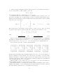
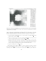
In electromagnetic scattering problems one is interested in what happens when an electromagnetic wave (incident wave or excitation) f inc encounters an obstacle — of finite
extension mostly — which has propagation properties different from surrounding space
(fig. 2.1).
This results in the obstacle producing a scattered field f sc , which can be found by
solving the boundary value problem
D(f sc ) = d
(2.1)
for an inhomogeneity d caused by f inc . Often the total field f tot resulting from the
scattering process is of interest. For linear problems this is the superposition of the
incident and the scattered wave
f tot = f inc + f sc .
(2.2)
In the following section we will have a look at the field equations underlying electromagnetic waves.
Figure 2.1: Scattering problem. An incident wave f inc encounters an obstacle; a scattered
wave f sc results.
2.2
Field Equations
Electromagnetic theory is based on Maxwell’s equations
~ =−
curl E
∂ ~
B
∂t
~ = ~j0 + ~jc +
curl H
17
(2.3a)
∂ ~
D
∂t
(2.3b)
~ = ρ0 + ρc
div D
(2.3c)
~ =0
div B
(2.3d)
where additional dependencies are given by the constitutive relations. For linear, homogeneous, and isotropic media they are
~ = µH
~
B
(2.4a)
~ = εE
~
D
(2.4b)
~
~jc = σ E.
(2.4c)
Harmonic time dependence is used and time dependent quantities are represented as
phasors f ; the time value can be obtained by f (t) = <(f e−iωt ). This yields the complex
time harmonic Maxwell equations
~ = iωµH
~
curl E
(2.5a)
~ = ~j − iωε0 E
~ = ~j + (σ − iωε)E
~
curl H
0
0
(2.5b)
~ =ρ
div ε0 E
0
(2.5c)
~ =0
div µH
(2.5d)
where (2.5c,2.5d) are derived from (2.5a,2.5b). For investigation of the propagation of
electromagnetic waves it is usually assumed that the sources generating a field are outside
the domain considered. For such domains the Maxwell equations are homogeneous and
the Helmholtz equations
~ =0
(4 + k 2 )E
(2.6a)
~ =0
(4 + k 2 )H
(2.6b)
p
can be derived. k = ω 2 µε0 is the wave number of the medium.
An additional condition, which is necessary to guarantee the physical relevance of
the solutions to (2.5) and (2.6) as well as the uniqueness of the solution of (2.1), is the
radiation condition. It can be looked upon as a boundary condition for infinity and limits
the asymptotic behavior of the fields. For 3D problems it is
lim r[
r→∞
∂f (r)
− ikf (r)] = 0
∂r
(2.7)
and for 2D problems
lim
ρ→∞
√ ∂f (ρ)
ρ[
− ikf (ρ)] = 0.
∂ρ
(2.8)
f stands here for any of the field components. The radiation condition states that all
sources of the field are within a finite distance of the origin. However, it is not satisfied
for some idealized solutions, like the plane wave.
Inhomogeneous space is divided into several homogeneous domains Di , each of which
is characterized by (2.4) with µi , εi and σi . Applying (2.5) to the boundary ∂Dij leads
18
to the boundary conditions
~ i = ~n × E
~j
~n × E
i
(2.9a)
j
~ = ~n · ε0j E
~ +ς
~n · ε0i E
0
(2.9b)
~ i = ~n × H
~j +α
~n × H
~0
(2.9c)
i
j
~ .
~ = ~n · µj H
~n · µi H
(2.9d)
ς 0 is a surface charge on the boundary and α
~ 0 is a surface current along the boundary.
2.3
Choices for the 3D MMP Code
The 3D MMP code helps solve electromagnetic scattering problems with harmonic time
dependence within piecewise linear, homogeneous and isotropic domains (2.4) without
impressed sources (~j 0 = 0, ρ0 = 0, ς 0 = 0, α
~ 0 = 0). Using the trial method formalism of
chapter 1, operator equation (1.2) can be identified with the Helmholtz equations (2.6),
and equation (1.3) corresponds to the boundary conditions (2.9).
In the MMP programs the field itself is the primary quantity and is expanded directly.
The basis functions fj are the complex vector valued functions
~ r)
E(~
fj = ~
(2.10)
H(~r)
where ~r is a point in three-dimensional space. Usually closed form solutions of Maxwell’s
equations are used, mostly multipole solutions in cylindrical and spherical coordinates
(2D- and 3D-multipoles).
The excitation f inc is itself a solution of the Helmholtz equations and therefore of
the same type as the expansion functions. As a consequence, the inhomogeneity can be
written as
h = −LfN +1 .
(2.11)
The equations are obtained with the generalized point matching technique. The expansion functions are matched in discrete matching points on the boundary. As long as
the boundary is relatively smooth, the functions behave well on it and its discretization
is, within limits, independent of the choice of the origins of the expansions. A model of a
scattering problem consists therefore — apart from additional data like media properties,
frequency, etc. — of a set of matching points and a set of expansion functions (fig. 2.2).
Usually, more than just one domain is used. The formalism described in chapter 1
can easily be adapted by making the single expansion functions valid in only one domain.
The expansion functions for domain Dj are
fi in Dj and on ∂Djk
fi |Dj =
(2.12)
0 in Dk (j 6= k)
and the boundary conditions are enforced on all ∂Djk .
Other equations than the boundary conditions can be added to the overdetermined
system of equations.
19
Figure 2.2: MMP model of a scattering problem. The ×’s denote origins of multipoles
or other expansions, the ⊥’s matching points.
The system of equations is
[aji ]p [ci ] = [bj ]p
(j = 1, . . . , M ; i = 1, . . . , N ).
(2.13)
The number of equations M ranges between 2 to 10 times the number of unknowns N
depending on the type of the problem and the quality of the model. The system is solved
by a direct orthogonal method which yields a least squares result. Bearing (2.11) and
(2.2) in mind and with regard to chapter 5, (2.13) is favorably written in the augmented
form
ci
[aji , −bj ]p
=0
(j = 1, . . . , M ; i = 1, . . . , N ).
(2.14)
1
All expansions — including the excitation — can be treated in the same way.
Once the unknowns ci have been determined, the residual errors on the boundary and
the field values can be evaluated in arbitrary points. The results are usually presented
as error distributions on the surface and as plots of the field f tot on rectangular grids.
Whereas the determination of the parameters is expensive in terms of both computational
time and required memory, the cost for computing errors and plots is usually quite small.
20
3 Expansion Functions
3.1
General Remarks
The expansion functions used for the MMP programs are solutions of both Maxwell and
Helmholtz equations (2.6). The expressions for the expansions currently implemented in
the 3D MMP main program can be found in appendix C. For deductions please consult
textbooks [23, 24, 25]. In the following, some basic principles underlying the choice of
expansions in the MMP programs are discussed.
The demands on expansion functions for analytical and for numerical purposes are
different. An analytical expansion in the form of (1.4) is generally infinite. It is important
that the expansion be complete, i.e., that the difference between approximate and exact
solution disappears as N → ∞. Usually eigenfunctions of the differential operator in
various systems of coordinates form natural complete bases.
In numerical computations, it is more important that the field can be modeled with
as few functions as possible and the error quickly drops below a certain limit. The
purely analytical approach may not converge fast enough. Completeness in form of
convergence for N → ∞ is secondary for numerical expansions and may even have
to be sacrificed. As a consequence, different criteria for choosing the basis functions
are needed. This is somewhat simplified by the fact that the scope of numerical field
computation is only quantifying largely known problems and not discovering new effects
(though it has to be admitted that even simple electromagnetic problems can produce
stunningly complex results). The loss of completeness is not as severe as it might seem,
because the functions in everyday problems are usually better behaved than those in
a mathematician’s imagination. Singularities mostly enter through idealizations in the
modeling process and can be disarmed.
Another criterion for the choice of expansion functions is that of user friendliness
and implementation. A few types of expansion functions should be flexible enough to be
used for a wide range of problems, and they should also be fast to compute. Therefore
closed form solutions with functions that can easily be evaluated are preferable.
3.2
Solutions by Separation of the Helmholtz Equations
Separation of (2.6a) or (2.6b) and a deduction of closed form expressions is possible in
several coordinate systems [26].
Expansions of a field in an infinite series of free space solutions in circular cylindrical
and spherical coordinates are very common in analytical approaches. Due to the high
symmetries of the respective coordinate systems they are very flexible, and the mathematical functions within them can be obtained numerically at a low computational cost
through recurrence relations. In simply connected, closed domains a single origin expansion of infinite order with Bessel functions is sufficient to express any field. In more
complicated, multiply connected domains with several complementary domains, an additional Hankel multipole expansion is required in each of the complementary domains.
21
The proof for completeness of a minimal base of this kind has been given by Vekua for
the 2D case in [27]; for the 3D case no corresponding theorem is known to the authors.
The numerical realization of this “single multipole” approach is only feasible for domains with a nearly spherical or cylindrical shape of the domain itself or its complementary domains; the origins of the multipoles have to be near the centers of these spheres
or cylinders. The more the shapes differ from this case, the slower the convergence is.
The key to more flexible use of multipoles is to base an expansion on multiple finite
(1)
(1)
hn or Hn multipoles (C.16) (or (C.8), or (C.10), respectively) with different origins. A
few heuristic rules are sufficient to keep the basis functions sufficiently independent even
for numerical purposes, because each finite multipole has only a relatively local influence
on the unknown field.
The highest orders and the number of multipoles are closely correlated: The fewer
orders, the more poles. In the MMP approach relatively few multipoles with high orders
are used (cf. chapter 8). In other implementations of the GMT, many monopoles or
filament currents in the 2D case or many dipoles in the 3D case are used [28, 29]. The
charge simulation method with its multiple point charges is an analogous example from
numerical electrostatics. The other, analytical, end of this road can be seen in the
continuous field or source distributions on the boundaries of the domains as they occur
together with spherically symmetric Green’s functions in the vector Kirchhoff integrals
of the Huygens principle.
In some cases, expansions with Bessel functions Jn or jn for the radial behavior, which
are called normal expansions, are more efficient than multiple multipoles. A normal
(2)
(1)
expansion can be seen as the superposition of incoming and outgoing (Hn and Hn
(2)
(1)
or hn and hn ) waves. The Bessel function is regular because the singularities at the
origin cancel each other out, therefore, the origin may be within the domain. Normal
expansions cannot be used multiply because they do not have a local behavior. As a
consequence they can only be used for nearly spherical domains.
Experiments with multipole and normal expansions in more complicated oblate spheroidal coordinate systems have also been made [5], but the necessary functions are much
more demanding to evaluate. Usually the field in domains with geometries where such an
expansion might be efficient is easy to expand with multiple spherical multipoles alone.
Expansions other than multipoles and normal expansions are denoted as special expansions, mainly because they are less common. The plane wave is a solution in Cartesian
coordinates and often used as excitation. In addition, closed form solutions already fulfilling some boundary conditions can be useful, e.g., waveguide modes for rectangular
and circular waveguides. Another form of special expansions is discussed in the following
sections.
3.3
Solutions by Integration
A different approach to find solutions of the homogeneous Helmholtz equations (2.6) is to
solve the inhomogeneous Maxwell equations (2.5) or the corresponding inhomogeneous
Helmholtz equations for sources outside the domain considered. Within the domain
this solution also satisfies the homogeneous Helmholtz equations. The sources can be
electric currents ~j 0 and charges ρ0 , but also their dual counterparts, magnetic currents
and charges, which are nonphysical at least for technical applications.
22
For currents the deduction is formally easiest to perform via the magnetic vector
~
potential A
~ = 1 curl A.
~
H
(3.1)
µ
It is obtained from
~ r) = µ
A(~
4π
Z
~j (~r0 )G(~r, ~r0 ) dV 0 .
0
where
(3.2)
0
G(~r, ~r0 ) =
eik|~r−~r |
|~r − ~r0 |
(3.3)
is the free space Green’s function. From (3.2), formulas for the field quantities can be
derived. It is obvious that these integrations can only rarely be performed analytically.
In most cases one has to employ numerical methods.
Such expansions are appropriate in cases where multipole expansions are extremely
inefficient, e.g., for structures with a high surface/volume ratio. A technically very
common example are thin wires (section C.1).
Also multipole functions of the previous section can be derived from a configuration
of infinitesimally small electric or magnetic sources at their origins.
Each expansion function for a domain is by (2.9) equivalent to a distribution of electric
and magnetic currents and charges on the entire boundary. Because the singularities of
the expansions are away from the boundary, this distribution is very smooth as long as
the boundary itself remains smooth. The coefficients are chosen in such a way that the
exact distribution is approximated as well as possible.
3.4
Connections
Another type of expansion function can be constructed by combining several expansions
into a macro. In the 3D MMP main program it is implemented as a connection, which
is the expansion function
K
X
f=
ck fk .
(3.4)
k=1
The parameters ck are given, mostly by a previous computation. Connections may be
nested, i.e., be used again within another connection. If the fk in (3.4) are expansion
functions for different domains, the connection becomes a multi-domain expansion.
There are several aspects under which connections can be useful
• More Complex Excitation Functions More complex excitation functions can
be defined as a superposition of simpler ones.
• Disturbed Problems An undisturbed problem often has higher symmetry than
the disturbed one. It is therefore easier to compute the undisturbed problem and
subsequently use the solution within the disturbed problem than modeling and
computing the whole disturbed problem.
• Successive Improvement The error in a problem can be minimized in one ore
more subsequent computations using previous results as excitation. An advantage
23
is that there are no direct dependencies between expansions at the various levels
of iteration as might be the case if all would be used at the same time.
• Splitting Problems Many problems can be split up into several almost independent parts. The parts may have a higher symmetry than the problem as a
whole.
3.5
Scaling
The range of numbers which is used by a particular expansion depends on the unit
system, on the type of the expansion and its mathematical functions, and on the way it
is used within a model. In order to compensate for this, an expansion function fi may
be scaled with a scaling factor s
fi → sfi
(3.5)
which is equivalent with a column scaling of [aji ]. There are several reasons for doing
this.
From the numerical point of view scaling influences the condition number of the matrix
and therefore the accuracy of the solution. However, no general scaling technique based
on the values of the matrix elements alone is known to improve the condition number
in all cases. In our implementation an additional difficulty is that not the entire matrix
[aji ] is known at a time (cf. chapter 5).
A common way out is to scale for a physical “significance”, which should be about
the same for all expansion functions. However, its definition is not quite clear. It can be
a global one, like total radiated power, or a local one, like the size of the field values in
the closest matching point, which for multipoles depends mainly on their distance from
its origin.
A practical reason for scaling is the interpretation of the resulting parameters ci . The
convergence of the parameters within a single multipole can show whether the highest
order is sufficient, and one may want to compare different expansions by the size of their
parameters.
Practice has shown that it is usually unnecessary to scale the columns for numerical
reasons. Furthermore, the influence of the actual model and of the choice and location
of the expansions on the condition of the matrix is dominant. The numerical accuracy
of the parameters plays only a minor role as the size of the residual errors gives a good
control over the solution. However, the advantages for interpretation have been leading
to the scaling of the expansions as currently implemented.
In the 3D MMP code, scaling is done between electric and magnetic modes and
between different orders and degrees within a single multipole or normal expansion. For
some expansion types an extra scaling factor can be specified (chapter 10 and appendix
C).
24
4 Equations
4.1
Boundary Conditions
After having the appropriate basis of expansion functions for the field, we shall discuss
the conditions to be satisfied in order to get a system of equations. On the boundary
∂Dij between domains Di and Dj the boundary conditions are
~j
~ i = ~n × E
~n × E
i
j
~ = ~n · ε0 E
~ +ς
~n · ε0i E
j
0
i
j
~ = ~n × H
~ +α
~n × H
~0
~ i = ~n · µj H
~ j.
~n · µi H
~n is a vector normal to the surface. Between two general domains there are supposed
to be no unknown surface charges or currents, therefore α
~ 0 = 0 and ς 0 = 0. In the
coordinate system {~en , ~et1 , ~et2 } of a matching point this leads to the six equations
ε0i E in = ε0j E jn
(4.1a)
E it1 =
E jt1
(4.1b)
E it2
E jt2
(4.1c)
=
µi H in = µj H jn
(4.1d)
H it1 =
H jt1
(4.1e)
H it2
H jt2
(4.1f)
=
The equations for the normal components are dependent of those for the tangential
components and only four linearly independent conditions remain. But the linear dependence is lost again when a residual error in the boundary conditions is admitted. In this
case it is better to explicitly use all of the boundary conditions in order to distribute the
error more evenly among the components of the field.
4.2
Perfectly Conducting Surfaces
Within perfectly conducting domains the field is zero. No expansion has to be made
for those domains, which are therefore not domains in the MMP sense. Because of the
surface currents and charges, the conditions to be satisfied on the boundary of a perfectly
conducting domain reduce to
E t1 = 0
(4.2a)
E t2 = 0
(4.2b)
µH n = 0.
(4.2c)
Again (4.2c) is dependent of (4.2a, 4.2b). Those equations of (4.1) which have been
omitted can serve to determine the unknown electric surface charge and current.
25
4.3
Imperfectly Conducting Surfaces
The surfaces of domains with a high refractive index can be modeled with surface impedance boundary conditions [30]. The field within the refractive domain Dj is locally
approximated by vertically entering plane waves; explicit expansions for the field within
the domain are not made. Like the perfectly conducting domains these are not domains
in the MMP sense. The surface impedance boundary conditions are
~ i ) · ~en = Zj ~en × H
~ i.
~ i − (~en · E
E
(4.3)
q
Zj = µj /ε0j is the wave impedance of the refractive domain. In the coordinate system
of the matching point the equations are
E it1 = −Zj H it2
(4.4a)
E it2
(4.4b)
=
Zj H it1 .
For validity it is necessary to make sure that the waves entering in a place do not exit
again in another place on the boundary. As a consequence the boundary must satisfy a
condition
s
2
R
(4.5)
δj =
ωµj σj
where δj is the penetration depth or skin depth and R the smallest radius of curvature
at a point of the boundary or the smallest thickness of the domain. In practice, this
means that surface impedance boundary conditions are only applicable on surfaces of
well-conducting domains, usually denoted as imperfectly conducting surfaces.
For Zj approaching zero, which is the case for a high permittivity εj or a high conductivity σj , the surface impedance boundary conditions turn into those for perfectly
conducting surfaces (4.2a, 4.2b). For a detailed deduction see e.g. [30].
4.4
Constraints
The approximation of the exact solution f of the problem and the admission of an error
function η on the surface can lead to undesired effects. A small local error can accumulate
over the surface to a large overall error, which in some cases leads to violation of laws on
a larger scale. A remedy is to introduce additional equations with a high weight, e.g. in
form of integrals
Z
g(f tot ) d· = 0
(4.6)
imposed on a function g of the total field f tot . In the MMP code these additional
conditions are called constraints or special conditions. Note that g has to be linear in the
components of f tot so that the integral can be added to the equations as
N
X
Z
ci
Z
g(fi ) d · +
i=1
26
g(f inc ) d· = 0.
(4.7)
As a consequence, power integrals cannot be used, although a discontinuity of the power
flux through a boundary is a common error.
Constraints are only rarely used in MMP models. A different technique to overcome
such difficulties is to give a high weight to the boundary conditions in certain matching
points in order to locally “zero” the error function.
4.5
Weighting
The weight affects the importance of an equation in an overdetermined system of equations. Thus, it is necessary to compensate for various differences which otherwise would
not be relevant:
• In the MKSA system or SI, which is used throughout in the program, the electric
and the magnetic field do not have the same numerical magnitude.
• The boundary conditions for the normal components (4.1a, 4.1d) are multiplied
with actual values for ε0 and µ.
• In order to be compatible with the error method and the projection method, the
equations in the matching points need to be multiplied with a weight wk which is
a combination of the square root of surface sk of the element associated with the
matching point k and a weighting function w(r)
√
(4.8)
wk = sk w(rk ).
w(r) can be used to emphasize some regions or points more than others and to
“simulate” exact equations.
If the optimum weighting factors, which depend on ε0 , µ and Z, are different for the
domains bordering the matching point, the geometric mean is used because of the good
experiences which have been made with this choice. The actual boundary conditions in
the matching point k on ∂Dij are consequently
wk q
1
|ε0i ε0j |
(ε0i E in − ε0j E jn ) = 0
(4.9a)
wk (E it1 − E jt1 ) = 0
(4.9b)
wk (E it2
E jt2 )
−
=0
p
|Zi Zj |
wk p
(µi H in − µj H jn ) = 0
|µi µj |
q
wk |Zi Zj |(H it1 − H jt1 ) = 0
q
wk |Zi Zj |(H it2 − H jt2 ) = 0
(4.9c)
(4.9d)
(4.9e)
(4.9f)
and for perfectly conducting surfaces
wk E it1 = 0
27
(4.10a)
wk E it2 = 0
wk |Zi |H in
(4.10b)
= 0.
(4.10c)
The surface impedance boundary conditions are
wk (E it1 + Zj H it2 ) = 0
(4.11a)
wk (E it2
(4.11b)
−
Zj H it1 )
= 0.
Constraints are mostly added to the system of equations with a very high weight in
order to simulate exact equations (section 5.4).
28
5 Solving the System of Equations
5.1
General Remarks
The complex system of equations which has been set up in the last few chapters is
[aji ]p [ci ] = [bj ]p
(j = 1, . . . , M ; i = 1, . . . , N )
(5.1)
Ac = b.
(5.2)
or more simply
As the expansion functions are produced using recurrence relations, A naturally is computed row by row. Scaling of the columns and weighting of the rows has already been
discussed in sections 3.5 and 4.5. The parameters are determined for just one right-hand
side as only one excitation is considered at a time. The number of rows M is usually
about 2 to 10 times the number of unknowns N . The equations are solved by least
squares, i.e., by minimizing the 2-norm of the residual vector |[ηj ]|2 = |Ac − b|2 . In most
cases N and M are so large that the time needed for computing the rows is considerably
smaller than the time needed for solving the matrix equation.
Different algorithms exist for solving the linear system. Each is a tradeoff between
numerical qualities, memory consumption, computational time and the desired results.
The algorithms used in the 3D MMP main program are all modifications of LINPACK
routines; a detailed description can be found in [31].
Figure 5.1: Typical shape of the rectangular system matrix A (M = 2 . . . 10N ) and the
triangular matrix R or X for a problem with 3 domains.
5.2
Solution with Normal Equations
The classical method to solve (5.2) is to form the normal equations and solve the square
system
A∗ Ac = A∗ b.
(5.3)
29
Because A∗ A is hermitian, only the upper triangle needs to be stored. It is favorably
formed by subsequently summing up the exterior products of the rows
"N
#
M
X
X
∗
∗
A A=
[aji ] [aji ] .
(5.4)
j=1
i=1
Positive definite matrices can be factorized into triangular matrices using the Cholesky
factorization
A∗ A = X ∗ X
(5.5)
where X is upper triangular. The vector of unknowns c can be found by successively
solving the triangular systems
X ∗ z = A∗ b
(5.6)
and
Xc = z
(5.7)
using forward and backward substitution respectively. As already stated in section 2.3
it is easier to use the augmented system
c
0 0
A c = [A, −b]
=0
(5.8)
1
with the Cholesky factor
0
X =
X
0
z
ρ
.
(5.9)
z is the same vector as in (5.6) and can be used to calculate c with only one single backward substitution (5.7). ρ is the norm of the residual vector and serves as an immediate
measure for the quality of the solution.
For large M and N the formulation of the — complex — normal equations (5.3) needs
M N 2 /2 times 8 FLOPS, the Cholesky factorization requires N 3 /6 times 8 FLOPS and
the back-substitution needs N 2 /2 times 8 FLOPS. A FLOP is one floating operation,
usually an addition or a multiplication.
The matrix A∗ A is equivalent to the one obtained with the projection or error method.
However, practice shows that it has very poor numerical properties. Its condition number
is the square of the one of A. Although solving the least squares problem with the normal
equations is the fastest method, it also is numerically the worst, and it is only feasible for
rather small problems. For larger problems the matrix can numerically lose its positive
definiteness during factorization and the algorithm will then come to a premature end.
Nevertheless this algorithm has been introduced into the 3D MMP program for small
benchmark problems where numerical problems do not yet arise.
5.3
Solution with Orthogonal Transformations
A much better way to solve the least squares problem is to use the QR decomposition
A0 = QR0
or
30
Q∗ A0 = R0
(5.10)
to compute an upper triangular matrix R0 directly from A0 . Q is unitary and therefore
does not increase the condition number of A0 . As
∗
∗
X 0 X 0 = R0 R0
R0 is equivalent with X 0 to within a factor of eiϕ per row.
For practical use there are several ways of obtaining R0 . The one fitted best to our
needs is an algorithm based on Givens plane rotations. A Givens transformation is the
unitary M by M matrix G(i, j) which is different from the unity matrix I only in columns
and rows i and j respectively


I


c
s



I
with
c2 + s∗ s = 1.
(5.11)
G(i, j) = 


∗


−s
c
I
The product G(i, j)∗ A performs a rotation in the i-j plane of A. If c and s are chosen
properly, it can be used to selectively introduce a zero into the element akj of A
c
s
aij
af
ij
·
=
(5.12)
−s∗ c
akj
0
with
|aij |
c= p
|aij |2 + |akj |2
and
s=
−a∗ akj
p ij
|aij | |aij |2 + |akj |2
(5.13)
The procedure used in the 3D MMP main program is an adaptation of a LINPACK
f0
algorithm for updating QR factorizations, i.e., for computing the modified matrix R
0
0
from R when a row x = [akj ], (j = 1, . . . , N + 1) is added to the original matrix A .
Zeroes are introduced into x in the following fashion:
Starting with an initially empty triangular matrix, the rows of A0 can successively be
updated. Finally we end up with R0 . Note that it is not necessary to keep the entire
matrix A0 in memory. Storage is required only for R0 , which is dense, and for the rows
currently being updated. These rows are discarded during updating. For determination
of the residuals they have to be recomputed.
This algorithm does not fail in case of a bad condition of A0 . Problems with more
than 1500 unknowns have been solved with good results.
The QR-factorization of a matrix A needs M N 2 /2 times 20 FLOPS. Other orthogonalization algorithms, e.g., those using Householder transformations, are faster, but need
the entire matrix A and, therefore, considerably more memory.
31
5.4
Exact Equations
In chapter 4 it was shown that is useful to satisfy some of the equations exactly, i.e., to
impose constraints on the least squares problem. An attractive alternative to the direct
elimination of these equations is to treat them as ordinary least squares equations with a
high weight. A tradeoff has to be made between getting the residuals of these equations
sufficiently small and not increasing too much the condition number of A0 . An extra
weight of 106 usually gives good results. An error estimation and numerical examples
can be found in [33].
5.5
Parallelization
With the growing complexity of the problems one wants to solve, computational time
explodes. Most of it is spent in the updating routine. Compared to this, the time for
computing the rows of A0 is negligible. Improving performance of the program therefore
means in the first place improving the speed of the updating algorithm. The complexity
of the source code of the program behaves oppositely: most of the program consists of
routines for computing the functions and the rows, whereas the code which performs the
actual updating is only a very small part.
One of the most efficient ways to speed up a code is to parallelize it. The approach
presented here is for implementation on a coarse grained network of processors and parallelizes only the updating algorithm. It has been used on transputer networks, which
provide high computational power at a low price. They allow to build very cheap and
yet extremely powerful machines, which can be entirely dedicated to a task. For a discussion of the usage of transputers for electromagnetic field calculation and the hardware
currently in use, see [34].
f0 are only affected
A look at the updating algorithm shows that the first k rows of R
0
by the first k columns of the updated row [aij ]. R is divided into N trapezoidal shares
R1 , . . . , RN of “equal” size, which means that the updating time is about the same for
each part. The shares are residing on different processors (cf. fig. 5.2), which form a
pipeline structure.
The part of the program which produces the rows and does input and output does not
have to be parallelized and can reside on the root processor. This is the major portion
of the code. The root processor can also take a share of R0 ; however, its optimum
size depends on the size of the problem being solved and on the size of the pipeline.
Computation of the rows plus updating of this share should take the same time as
updating of one of the other shares. If the share is larger, the rest of the pipeline has
to wait for the root processor; if it is smaller, the processor is not fully occupied. Both
reduce performance. The procedure for the updating on one processor i having a share
Ri of ni rows is the following:
1. Get x from processor i − 1
2. Update the first ni columns of x into Ri
3. Pass the remaining modified rest of x on to processor i + 1
4. Get next x (go to step 1)
32
Figure 5.2: The triangular matrix R0 is divided into trapezoidal parts residing on different
processors in a pipeline structure. The root processor holds the major, not parallelized
part of the program, the other processors just small updating programs. Only short
vectors have to be passed on down the pipeline.
Parallel speedup does not depend quite linearly on the number of processors. The procesf0 is sufficiently filled; optimum
sors towards the end of the pipeline are unemployed until R
parallelism is reached only after N rows have been updated. For larger problems — where
it is important after all — exploitation gets better.
Back-substitution is not parallelized, but only takes very little time. It starts on the
last processor in the pipeline and propagates on to the upper ones.
A big advantage of this approach is that it can easily be adapted to pipelines with
an arbitrary number of transputers without changes in the program’s structure. Therefore the hardware can be adapted to the problem size. For larger problems, additional
processors can be attached to the pipeline, which give it more memory as well as more
computational power.
Evaluation of errors and field values (chapter 6) is not parallelized and is done on the
root processor. As this processor also has to hold the large part of the program as well as
the rest of the data, it is favorable to use a processor with more memory and, possibly,
more computational power than the others.
33
6 Evaluation of Results
Once the unknown parameters have been determined it is easy to evaluate the residual
error of the boundary conditions or the components of the field in arbitrary points on
the boundary. For common problems the computational time for error and field values
is negligible compared to the time needed for determining the unknowns.
6.1
Residuals and Errors
The error distribution on the boundary is an important aspect in estimating the quality
of the result (see chapter 8). More useful than looking at the residuals of the field
components is to introduce one single error value ρk for a matching point k on ∂Dij as
an indicator for the mismatching in this point. It is the average of the residuals defined
by the boundary conditions (4.9)
"
i
j
2 2
1 |ε0i E n − ε0j E n |2 i
i
j j 2
+
+
−
E
−
E
ρk =
E
E
t1
t2
t1
t2 6
|ε0i ε0j |
(6.1)
2 2 |µi H in − µj H jn |2 i
i
j j + |Zi Zj |
+ H t1 − H t1 + H t2 − H t2 |µi µj |
~
rk
and for perfectly conducting surfaces with the boundary conditions (4.10) respectively
i
1 h i 2 i 2
2
2 i 2 ρk =
E t1 + E t2 + |Zi | H n .
(6.2)
3
~
rk
For surface impedance boundary conditions the error is
ρ2k
i
i
1 h i
i 2
i 2 E t1 + Zj H t2 + E t2 − Zj H t1 .
=
2
(6.3)
~
rk
In points with reduced boundary conditions only the matched components are averaged.
Note that the weight wk defined in (4.8) does not affect the error value. Otherwise a
denser discretization would reduce the error due to the smaller surface elements.
If the original matrix [aji ] is not stored for saving memory, the rows have to be recomputed. In addition to the original matching points, the error may also be determined
between them. However, in case of overdetermined systems of equations, the error between matching points does not differ much from that in the matching points themselves
provided that the system is sufficiently overdetermined.
6.2
Field
The total field in a field point ~r is
f (~r) =
N
+1
X
i=1
34
ci fi (~r).
(6.4)
For evaluation of only the scattered field f sc the incident field f inc = fN +1 can be
omitted.
A very useful feature for the production of plots within regions with several domains
is the automatic detection of the domains. In order to determine the domain of a field
point specified by the coordinates (x, y, z)T , the next matching point is determined.
With the convention that the surface normal ~en for a matching point on Dij is always
pointing from Di into Dj , the domain can be determined in practically all cases. For the
rare circumstances where this does not work, additional dummy matching points can be
added, in which no boundary conditions are enforced.
6.3
Integrals
In addition to the fields, integral quantities like voltage, flux, power flux, etc., are of
interest. The integrals usually have to be evaluated numerically and are implemented as
Riemann sums (section 10.7).
35
7 Symmetries
7.1
Boundary Value Problems and Symmetry
The geometry of boundary value problems is often symmetric, i.e., invariant to certain
symmetry transformations in space. Exploiting these symmetries pays off in a considerable reduction of computational time and memory requirements and, furthermore,
brings numerical advantages. Symmetries are also an easy way of introducing perfectly
conducting infinite planes into a model.
The mathematical tool needed for treatment of symmetries is group theory. A complete and understandable description of its application on boundary value and eigenvalue
problems is given in [35, 36, 37, 38, 39]; in this section only the consequences are outlined.
A linear symmetry transformation in n-dimensional space is represented by a n by
n matrix D. The various symmetry transformations which are applicable on a given
geometry can be seen as representations of the elements s of a group G. They are
consequently written as D(s). A matrix A has the symmetry of the group G if
D(s)A = AD(s)
∀s ∈ G.
(7.1)
For the matrix equation in a boundary value problem
Ac = b
equation (7.1) means that a symmetry transformation of the boundary values b is equivalent to the same transformation of the result c.
Group theory shows that a transformation T can be found which transforms A into a
e (fig. 7.1). The number and the size of the blocks is determined
block diagonal matrix A
by the group G. The transformations T are tabulated for the most common symmetry
groups.
As a consequence, the boundary value problem splits up into K smaller symmetry
adapted ones, which can be solved separately at a lower overall expense. Note that it is
not necessary for the boundary conditions to be symmetric!
Ac = b
→
Ak c k = bk
(k = 1, . . . , K)
(7.2)
The Ak usually have a better condition number and are, at any rate, numerically better
due to their lower dimension. An additional reduction of problem size takes place if some
symmetry components bk of b are equal to zero because of a symmetry of the excitation.
Therefore, the corresponding part of the problem has only the trivial solution ck = 0.
In homogeneous boundary value problems (eigenvalue problems) splitting the problem
into symmetry adapted ones helps to separate modes and especially degenerate solutions.
Instead of explicitly performing the transformation T on A, it is also possible to
directly set up the matrices Ak using symmetry adapted expansion functions.
7.2
Reflective Symmetries in the 3D MMP Code
In the 3D MMP code one or more reflective symmetries about the coordinate planes
X = 0, Y = 0 and Z = 0 of the global coordinate system are implemented. Due to
36
Figure 7.1: If A has the symmetry of a group G, a transformation T can be found which
e The number and the size of the blocks Ak
transforms A into a block diagonal matrix A.
is determined by G.
the orthogonality of these planes, the consideration of symmetries can be made quite
intuitively for one plane of symmetry at a time.
With respect to one symmetry plane a scalar field f can be split up into an even and
an odd component f + and f −
f = f+ + f−
(7.3a)
1
[f (+P ) + f (−P )]
2
1
= [f (+P ) − f (−P )] .
2
f+ =
(7.3b)
f−
(7.3c)
+ and − denote the even and odd components, +P and −P stand for a point and its
reflection.
If the field is only defined in a domain which is not intersected by a symmetry plane,
it is also possible to obtain the even or odd field in the reflected domain by
f + (−P ) := f (P )
and
f − (−P ) := −f (P ).
(7.4)
In the 3D MMP code there is no difference made between domains which are or are not
intersected, therefore (7.3) is always used.
For electromagnetic vector fields, additional dependencies between the components
have to be taken into account. Because Maxwell’s equations are invariant with respect
to reflections about a plane, the components must transform either like
E⊥ (+P ) = −E⊥ (−P )
Ek (+P ) = Ek (−P )
H⊥ (+P ) = H⊥ (−P )
Hk (+P ) = −Hk (−P )
(7.5)
E⊥ (+P ) = E⊥ (−P )
Ek (+P ) = −Ek (−P )
H⊥ (+P ) = −H⊥ (−P )
Hk (+P ) = Hk (−P )
(7.6)
or like
37
Figure 7.2: MMP model of a symmetric boundary value problem with one plane of
symmetry. Watch the different discretization in A and B. It is never necessary to put
matching points onto symmetry planes.
due to the duality of the electric and magnetic field. The index ⊥ stands for the component of a vector perpendicular to the plane, k for the one parallel to the plane. For
the 3D MMP code, an electromagnetic field is defined to be even about a plane if (7.5)
is true and odd if (7.6) holds. On the symmetry plane itself for an even field
E⊥ = 0
and
Hk = 0,
(7.7)
Ek = 0
and
H⊥ = 0
(7.8)
is valid, and for an odd field
is valid. As a result, the problem
Ac = b
with respect to one reflective plane splits up into an even and an odd problem
A+ c+ = b+
and
A− c− = b− .
A+ and A− can be set up directly and each have only approximately half the number
of parameters and equations of A. The field is evaluated by summing up the symmetry
components
N
+1
N
+1
X
X
+
−
c+
f
+
c−
(7.9)
f=
i i
i fi .
i=1
i=1
Above considerations can be superposed for three orthogonal planes of symmetry.
The inhomogeneity and the solution split up into eight symmetry adapted components
f = f +++ + f ++− + f +−+ + f +−− + f −++ + f −+− + f −−+ + f −−−
b = b+++ + b++− + b+−+ + b+−− + b−++ + b−+− + b−−+ + b−−−
38
(7.10)
(7.11)
and the whole problem divides into the eight parts
A+++ c+++
A+−+ c+−+
A−++ c−++
A−−+ c−−+
=
=
=
=
b+++
b+−+
b−++
b−−+
A++− c++−
A+−− c+−−
A−+− c−+−
A−−− c−−−
=
=
=
=
h++−
h+−−
h−+−
h−−− .
(7.12)
Each of these symmetry adapted matrices has only one eighth of the number of rows and
columns of the original problem.
For impact of the symmetry on the problem imagine that an MMP model is symmetric
(fig. 7.2).
A nonsymmetric expansion can be symmetrized with (7.3b) and (7.3c). An expansion
and its reflected counterpart produce the same symmetrized functions, so only one of
them has to be considered. Expansions with origins on the symmetry plane needs special
treatment. If it is properly oriented, it can already be even or odd about the plane and
consequently adapted to one of the symmetries. It is important that it enters only A+ or
A− respectively. In the wrong matrix it will produce a zero column, and the matrix will
become singular. Each plane of symmetry in which a multipole or normal expansion lies
leads to a reduction of the number of its parameters by a factor of 2. But if the expansion
is not properly oriented, all functions are symmetrized, and the expansion will enter both
A+ and A− with the full number of coefficients. Because normal expansions must not be
used multiply, their origin has always to be on the intersection of all symmetry planes.
The matching points can be treated by analogy. In a point and in its reflected counterpart, the values of a symmetric field are identical to a possible change of sign. This
results in the same equations for both points, and, by consequence, only one has to be
considered. In a point on a symmetry plane several of the components are zero because
of (7.7) and (7.8), and the symmetrization of the remaining components is simplified.
Note that it is never necessary to put a matching point on a symmetry plane (cf. fig. 7.2).
Zero rows in an overdetermined system of equations do no harm, but waste computing
time during updating.
Field points are in contrast to the matching points often lying on symmetry planes.
The reason is that the field is easier to interpret there due to the reduced number of nonzero components. However, the consideration of these symmetries does not save much
computational time, as evaluation of the field does not need much time anyway.
The choice of the principal domain, i.e., the side on which the expansions and matching points are considered, is not unique. In the MMP programs it generally assumed
to be the intersection of the positive half-spaces (i.e., the side on which the coordinates
are positive) of the symmetry planes involved. Having expansions on the other side of a
symmetry plane can result in a change of sign of the corresponding columns and, as a
consequence, of the parameters. Having matching points on the other side of the symmetry plane can affect only the sign of the corresponding rows and therefore does not
influence the solution.
39
8 Modeling and Validation
8.1
General Remarks
Creating good models of realistic configurations is an art that needs a great deal of experience and that is hard to express in words. This is especially true with regard to the
limits of numerical computations. The maximum size of problems which can be solved
by the 3D MMP code within a reasonable time makes strong simplifications indispensable in most cases. However, in this chapter these limitations are only of subordinate
interest. We assume that an appropriate idealized configuration of homogeneous, linear
and isotropic materials already exists. What remains to be done is mainly the transfer
of this structure into an MMP model with matching points and expansions.
As long as the boundary remains relatively smooth the actual location of the matching
points and the expansion is not very critical. Therefore the discretization of the boundary
and the setting of expansions (i.e., the choice of location and order) can be done almost
independently of each other. It has been found to be the simplest way to start with
the discretization of the boundary and subsequently set the multipoles. A special case
remain thin wires, which will be treated separately.
In the following, some simple rules for discretization and setting of expansions are
given. The rules are analogous for 2D and 3D models. They are not strict, but largely
based on experience gained from using MMP. They should be understood as heuristic
guidelines and sometimes may be violated. The more “generously” matching points and
expansions can be used, the less the model is prone to changes.
Before going more into details, a remark about the complexity of MMP models: The
size of the problems which can be solved is limited by available memory and computational time. Both depend for larger problems mostly on the size of the system matrix A
with dimensions M (number of rows) and N (number of columns). Memory consumption
Smem and CPU-time Tcpu behave as
Smem ∝ N 2
Tcpu ∝ M N 2 .
A given MMP model shall be improved by doubling the density of the matching points
and the orders of the multipoles. For a 2D model this results in a doubling of both M
and N , consequently
Smem → 4 Smem
Tcpu → 8 Tcpu .
For a 3D model the number of matching points and the number of unknowns quadruple,
so
Smem → 16 Smem
Tcpu → 64 Tcpu .
This shows that modeling in 3D is intrinsically much more difficult and critical than
in 2D and also is the reason why 3D problems usually look much simpler than 2D
40
ones. Given the multipoles as expansion functions, which are most efficient for surfaces
following coordinate surfaces, it makes clear why 3D MMP models mostly have rather
round shapes.
It also shows that for optimizing a model, it is more important to find a minimal
base of expansion functions, i.e., to set the multipoles optimally, than to minimize the
number of matching points. In the first steps of modeling, the matching points should
be rather too dense, because the model is easier to improve by changing the order of the
expansions alone.
8.2
Discretizing the Boundary
The boundary is discretized as an unordered set of matching points each of which represents conditions (4.9), (4.10) or (4.11). A part of the boundary belongs to each matching
point. It is represented by a rectangular surface element (fig 8.1).
Figure 8.1: Discretization of a surface with matching points, each of which is represented
by a rectangular surface element.
The expansion functions for the field are sampled on the matching points, which
should be dense enough to avoid aliasing not only of the incident field, but also of the
multipole expansions. The subsequent setting of the multipoles is based on the discretization. Thus the matching point distribution should be denser where more accuracy
is required.
Watch out for points near edges, corners or ends of thin wires! In these regions the
field is locally very high, but has little influence on the overall solution. The boundary
conditions have very high numerical values in these places because of the high field.
With the least squares algorithm the error in these points is unnecessarily reduced at
the expense of the error in other matching points. This can have a global influence on
the solution, which is then likely to produce a too small scattered field. It is therefore
advisable to keep the matching points away from these singularities or to round off the
boundary, where possible.
The error tends even to get higher in places where the curvature has a discontinuity
although the boundary itself remains smooth.
Domains of a geometrically complicated shape can be subdivided with fictitious
boundaries into several more simply shaped domains, all of which have the same electromagnetic properties (cf. fig. 8.2). On the fictitious boundary, i.e., within the original
41
Figure 8.2: Geometrically complex domains can be subdivided with fictitious boundaries.
domain, an error is allowed. Expansions may be found more easily, and sometimes normal expansions can be used (see below). In addition to enforcing boundary conditions,
in the 3D MMP main program the matching points are used for computation of errors
and for the automatic determination of the domain in which a field point with given
coordinates is lying. Dummy matching points, which do not contribute to the size of A,
may be added for these purposes.
8.3
Multipoles
Multipoles, or simply poles, are the most flexible expansions within the MMP code.
Their origins have to be set outside of the domain in which the field is modeled, i.e., in
the complementary domain.
If several poles are used for the same domain, special care has to be taken to avoid
dependencies between them. A multipole is characterized by its region of influence, i.e.,
the region within which it is able to efficiently fulfill boundary conditions. For a full
multipole, this region is a sphere with a radius of 1.2 to 1.4 times the distance to the
nearest matching point, this number also grows with the order of the pole. No other pole
should be within this region without the danger of numerical dependencies.
The matching points within the region of influence are denoted as associated matching
points. A matching point is usually associated to one, but not to more than two poles
for the same domain. For flat boundaries, the maximum angle under which the set of
associated matching points is seen from the pole should not exceed π/2.
The problem of finding origins for the multipoles can be visualized with a simple
analogy. Imagine the boundary of a domain being covered by as large as possible spheres
(or regions of influence) in the complementary domain each of which has a pole at its
center (figure 8.3). The spheres are “soft”, i.e., they can intersect or extend into the
domain to a certain degree.
Once the locations of the poles are known, the orders have to be determined. The
maximum order Nmax and degree Mmax of a multipole (cf. section 10.5) are bound by
the overdetermination factor and the sampling theorem.
The overdetermination factor of the matrix A, i.e., the quotient of the number of rows
M and the number of columns N , gives a lower limit for the order. This factor ranges
from 2 (for optimized models) to 10 (for rather safe models with respect to the matching
points). A good value is about 3, which in practice means one unknown parameter per
42
Figure 8.3: The boundary is covered with spheres, containing multipoles, within the
complementary domain.
associated matching point.
Figure 8.4: The largest angle between two matching points as seen from the origin of the
multipole determines the largest possible order and degree of the multipole.
The sampling theorem limits the maximum order Nmax and the maximum degree
Mmax through the largest angles which separate two neighboring matching points seen
from the origin of the multipole: φmax in the ~eϕ direction and θmax in the ~eϑ direction
Nmax <
π
φmax
and
Mmax <
π
.
θmax
(8.1)
If the sampling theorem is violated, the errors are usually very small in the matching
points, but large between them.
For a full expansion, which is invariant to rotations about its origin, Mmax is equal
to Nmax . Sometimes properly oriented reduced poles with Mmax < Nmax may be more
economical because they have less parameters. The region of influence of such a pole is
rather like a prolate spheroid.
The exact location of the multipoles and the choice of orders is usually not very
critical — at least not in “generous” models — and several arrangements can produce
43
good results. A fully automatized pole setting program for 2D static problems, which
implements the above principles and is based on the matching points, has already been
studied in [6]. Some relatively easy rules can already give a good base for subsequent
hand-optimization. Such features are now available for 3D modeling as well and are
implemented in the graphic interfaces [16].
8.4
Normal Expansions
Obviously many multipoles are needed around a finite domain, especially in 3D. Sometimes they can be replaced by a single normal expansion. Its location is not very critical,
as it does not have an as local behavior as a multipole. Usually the origin is chosen
somewhere near the center (fig. 8.5). Subdividing domains with fictitious boundaries
may simplify their use.
Figure 8.5: The poles around a domain can often be replaced by a normal expansion ◦.
Only one normal expansion may be made for a domain. If symmetries are used, the
normal expansion has therefore to be on the intersection of all symmetry planes, even if
this is not within the domain.
The use of normal expansions leads for many simply shaped domains to much fewer
unknown parameters, although its order has mostly to be very high.
8.5
Thin Wires
A long thin wire with arbitrary current distribution is made up of single segments (C.1)
(cf. fig. 8.6). In the thin wire expansion (C.4) only the continuity conditions (C.2) for
the current between the segments of one wire expansion are fulfilled exactly. As can be
seen in the analytical deduction, the segments have to be shorter than a quarter of the
wavelength λ; in practice λ/10 is a good choice. Moreover, the length of the segments
should be at least equal to the diameter of the wire.
The discontinuity of the charge distribution near segment junctions principally acts
as a point source, but is usually too small to be dangerous to nearby matching points.
However, keep them away from such junctions if you think they might exert a bad
influence on the solution.
Thin wire expansions are axially symmetric around their z axis. Therefore only one
line of matching points along the surface of the wire is needed and only the boundary con-
44
Figure 8.6: Thin wire expansion with matching points. Additional dummy matching
points may be necessary for the automatic detection of the domain.
~ in the direction of the wire may be posed. Unlike
dition for the tangential component of E
in the NEC code, where one does not work with overdetermined systems of equations,
more than one matching point is needed per segment. According to [40] two matching
points per segments are sufficient and their optimal positions can be estimated from
simple formulae that have been implemented in the 3D MMP code. Additional dummy
matching points around the wire are usually necessary for the automatic detection of
domains.
At open ends of the wire, the last matching point should have a distance of 1/3 to
1/2 segment lengths from the end. Otherwise the high error values near the end, which
are caused by the very high field values, will bring about a too small current on the wire
(see above and [41]). The current at the end has to be left freely floating.
If several wires are joined or if wires are joined to surfaces, the boundary conditions
are sufficient to guarantee good continuity also in these places. Tests have shown that it
is not even necessary to use the continuity conditions (C.2) for thin wires; the residual
errors on the boundary may even get smaller due to the higher number of parameters.
8.6
Symmetries
When reflective symmetries are used (cf. chapter 7), only one half of the model with
respect to each plane of symmetries has to be used. These are the expansions and the
matching points in the principal domain, which has been defined as the positive half-space
in regard of each symmetry plane, e.g., X ≥ 0 for a symmetry about X = 0.
To apply the above stated rules, always imagine the whole problem, which consists
of the discretized part and its reflections, and avoid dependencies between a multipole
and its reflected counterpart as between ordinary multipoles.
Make sure that the multipoles and normal expansions on a symmetry plane are
properly oriented, i.e., that always one of the basis vectors of their coordinate system
{~ex , ~ey , ~ez } is perpendicular to a symmetry plane. Otherwise no reduction of the number of parameters will take place for these expansions. The 3D MMP graphic editor
automatically adjusts the orientation of expansions upon request.
Normal expansions need to be on the intersection of all symmetry planes because the
reflected expansion can cause dependencies.
Matching points on the symmetry planes are not necessary and even inefficient, as
shown in chapter 7.
45
8.7
2D Problems
For 2D problems the rules for discretization and for setting poles are analogous to the
3D case. 2D poles have a less local behavior (logarithmic for zero orders and small
√
arguments, 1/ κρ instead of 1/kr for large arguments) and therefore are more exposed
to the danger of dependencies. On the other hand, in 2D more complex models can
be solved either with the 2D MMP package [4] that handles scattering and eigenvalue
problems or with 3D MMP for scattering.
The excitation of a 2D scattering problem is often a plane wave, which is oriented
in such a way that it is either transverse electric or transverse magnetic with respect to
the longitudinal axis of the problem. In order to reduce computation time and avoid
dependencies among the expansion functions, only the E- or H-parts of the expansions
may be used in these cases.
8.8
Validation
Validation of the model as an idealization of reality and validation of the computation
of a particular model are two different things. While the first is clearly beyond the scope
of this document, the 3D MMP code provides good facilities for the second.
The norm of the residual vector ρ = |η| is a direct result of the updating algorithm and
can give a first assessment of the overall error of the solution and of the error contribution
of the symmetry components.
The error distribution, a graphical representation of the errors in the matching points,
shows in which parts of the model the solution is good and in which it is poor. It is a
good basis for optimizing models. Moreover, the error between the original matching
points can be computed with dummy matching points, e.g., near edges, corners or ends
of wires. However, this is usually not necessary.
Field plots give a good impression of the qualitative correctness of the solution. Especially animated plots are very instructive and facilitate considerably a deeper understanding of what happens. Critical regions can quickly be zoomed in.
Convergence of the parameters of a multipole can show whether it is sufficient to
model the field and whether the order of the pole should be changed.
8.9
Improving a Model
Modeling is usually an iterative process. The result of a first computation may not
yet be satisfying, but it can give valuable hints towards an improved model. The error
distribution and the field plots give a good impression of which regions are important
for the solution and which are well modeled. In critical regions the matching points can
be placed more densely. At the same time the orders of the existing poles should be
augmented or more poles of smaller order be used.
Another possibility is to start a second computation, using as excitation a connection
with the solution of the previous problem. New multipoles can be added in critical
regions with less danger of dependencies with expansions of the previous computation
than without connections.
46
A third way is to increase the weight of the matching points in these regions. However,
this reduces the accuracy in other regions.
In some cases it may be necessary to “fix” the field in some places with highly weighted
matching points or to add constraints.
Last but not least, one can introduce fictitious boundaries when the computation is
considered to be much more accurate inside a domain than on its boundary. Above all for
complicated structures, this allows to achieve a much more balanced error distribution.
If fictitious boundaries have been introduced, moving these boundaries and varying the
weights of the corresponding matching points is helpful for getting more confidence in
the results.
47
Part II
User’s Guide of the Main
Program
48
9 Running the Main Program
9.1
Introduction
The 3D MMP main program is designed for solving time harmonic 2D and 3D scattering
problems for linear, homogeneous and isotropic materials. It is an implementation of the
theory described in chapters 1 to 7. Its capabilities are
• Computation of the parameters ci
• Computation of residual errors in matching points and constraints
• Evaluation of integral quantities
• Evaluation of complex amplitudes of the field f tot in arbitrary field points and on
rectangular grids.
Reflective symmetries are allowed about any of the coordinate planes X = 0, Y = 0
and Z = 0 of the global Cartesian coordinate system. With the Fourier transform utility,
computations can also be made for nonharmonic but periodic time dependence.
Input and output to the 3D MMP main program is made via ASCII files. Some
of these files can be prepared and viewed with graphic interface programs, which are
described in chapters 14 to 16.
The contents of the files are explained in the following chapters, the file formats are
listed in appendix D. All files are in FORTRAN list directed input format (*-format).
The programs are written in standard FORTRAN 77 and therefore use static memory
allocation. As a consequence the size of problems which can be computed is limited to a
maximum size determined by the parameters described in sections 20.3.2 and E.2.
9.2
Program Start
After preparation of the input file(s) start the program under Windows by double clicking the corresponding icon. After this, you sometimes obtain error messages issued by
Windows. Since these messages are not issued by the 3D MMP program, you have to
consult your Windows manual for more information. Note that the working directory is
defined as command line parameter. The predefined working directory is subdirectory
EX3D of the directory MMP3D, i.e., the place where the example input files are stored. If
you want to work on a different directory, you can click the icon of the 3D MMP editor
once, select “Properties...” in the menu “File” of the Windows “Program Manager”, and
modify the “Command Line” according to your needs. Instead of this, you can use any
of the features provided by Windows for running an application, for example, you can select “Run...” in the menu “File” of the Windows “Program Manager”. After sucessfully
starting the 3D MMP main program, the following messages and questions appear:
parallel version
number of t800 processors=xxx
3D MMP VERSION 3.3
49
Note: aaaaa is working directory
tasks:
0: EXIT
1: compute parameter file
2: compute standard error file
3: compute integrals
4: compute standard plot (p00..p49 files)
5: compute general plot (p50..p99 files)
6: compute extended error file
9: call routine USER
factorization method:
1: Givens
2: Cholesky
frequency:
1: single frequency
2: multiple frequency (Fourier transform)
input file number xxx:
xxx < 0: input files xxx=0..nome (Fourier Tr.)
xxx >=0: single input file xxx
The first two lines are suppressed when a single processor is used. Otherwise xxx
indicates the number of processors that have been found.
Usually the working directory is the current directory and aaaaa is a blank string.
Since Microsoft Windows does not allow running an application from any directory, the
Windows version of the 3D MMP codes allow to add the path of the working directory
to the command line. In this case, aaaaa is equal to this string and indicates where the
program looks for input files and writes output files.
On PCs the following questions have to be answered interactively, on UNIX systems
the options can also be entered on the command line.
tasks
This option specifies what the program shall do. The various tasks can be combined
and put into a single integer number, e.g., 124 for a computation of the parameters,
subsequent calculation of the errors and of a plot. In multiple frequency runs (see below)
these choices will be executed for each of the frequencies, i.e., 124 for the first frequency,
124 for the second frequency and so on.
Upon completion, the program will restart and be ready again for new tasks until
you explicitly exit with option 0. The exit option can also be used with the other task
options, e.g. as 1240. In the case of multiple frequency runs, the exit is performed after
the last frequency run only.
If errors, integrals or plot files have to be computed, either a computation of the
parameters must precede or a parameter file MMP PAR.xxx must be present.
If task 9 is chosen, the input and parameter files are read and subroutine user is
called. It can be modified for various custom expansions. In this version of the source
50
a version for interactive plotting with the graphic front end for UNIX workstations is
shown, but you are free to use subroutine user for your own needs.
Factorization Method
This option chooses the algorithm for calculation of the parameters. This is either the
updating algorithm with Givens plane rotation based on the matrix A0 or the Cholesky
∗
factorization based on A0 A, which is faster, but numerically inferior (see chapter 5) and
rarely used therefore. Note that the Cholesky factorization is incompatible with multiple
excitations.
Frequency
The MMP program can make computations for one or more frequencies in one run. For
a single frequency run the value cfreq from the input file (see chapter 10) is used, for
the multiple frequency run the problem is computed for each of the frequencies in file
MMP FOU.FRQ (see appendix D). Note that multiple frequencies are incompatible with
multiple excitations.
Input File Number xxx
The input and output files are numbered with an extension xxx.
For single frequencies with single excitations, the specified number usually is equal
to or greater than zero. It is used as extension for both input and output files. If it is
less than zero, it will be set to zero.
If multiple excitations have been defined in the input file the single frequency option
has to be selected because multiple excitations are incompatible with multiple frequencies.
In this case the output files (parameters, errors, plots, etc.) will be numbered from 000
to one less than the number of excitations. Already existing files will be overwritten.
For multiple frequency computations, if the specified number is equal to or greater
than zero, this input file is used for all frequencies, but the extension for the output files
loops from 0 to nome. (nome is specified in file MMP FOU.FRQ). If the specified number is
less than zero, the extensions for both the input and output files loop from 0 to nfreq.
In this way different input files and consequently different models can be used for the
different frequencies. If the corresponding input file is missing, the input file from the last
frequency step is reused, i.e., only one input file MMP 3DI.000 is necessary. The output
files will be numbered and overwritten like for multiple excitations.
51
10 Input
10.1
General Remarks
The main task in using the 3D MMP code is generating a reasonable input file MMP 3DI.xxx.
For more special problems, connection files MMP Cyy.xxx and frequency files MMP FOU.FRQ
are also needed. This chapter describes the contents of MMP 3DI.xxx and MMP Cyy.xxx.
The input file MMP 3DI.xxx is usually generated by a graphic input editor. For doing
special things and for slight modifications, editing the input file with a text editor may
be more practical.
FORTRAN implicit notation is used for the description of the parameters in the
input file. Integer parameters start with the letters i to n; real parameters with the
letters a, b, d to h and o to z; complex parameters start with the letter c and are entered
as a pair of real numbers, the first being the real part. The full format of the file is given
in section D.2.
10.2
Coordinates and Geometric Tolerances
All coordinates and vectors in the input file must be specified in the global Cartesian
coordinate system {~eX , ~eY , ~eZ }. For symmetry detection it has to be determined whether
a component of the radius vectors ~rpt (origin of a matching point) and ~rexp (origin of an
expansion) is equal to 0 or a component of the basis vectors of {~en , ~et1 , ~et2 } or {~ex , ~ey , ~ez }
is equal to 0 or 1. The tolerance for this is sklein and is currently 10−7 . It can be changed
in subroutine inicon in file ETC.F.
10.3
General Data
10.3.1
Type of Problem
The program is able to solve 2D and 3D scattering problems. Initializations for various
problem types depend on the value of iprob. Currently the following values of iprob
are used:
iprob
200..299
300..399
Problem Type
2D problems with translative symmetry in the Z direction
3D scattering problems
Within these ranges, you are free to use any values.
For 2D scattering problems with a plane wave excitation (iprob=200..299), the
propagation constants γ of the 2D-expansions will be initialized to the Z component
of the wave vector ~k of the incident plane wave. As a consequence, for 2D problems
with other excitations different problem numbers have to be used and the propagation
constants have to be declared with the expansions (see section 10.5).
52
10.3.2
Output on Screen and Output File
The amount of output on the screen and in the output file MMP M3D.LOG can be chosen
with msscr (screen) and msfil (output file). A description of this output and an example
is given in section 11.5.
msscr
0
1
2
3
4
Amount of Output
no output on screen (except questions at startup)
general output is written to the screen
same as msscr=1, but the current position of the program (matching
point number or field point number) is given and the error values are
shown
in addition to msscr=2 a graphic representation of the matrix is shown
if the number of columns does not exceed 80
in addition to msscr=3 a graphic representation of the rows is shown if
the number of columns does not exceed 80
For msfil, which determines the amount of output in the output file MMP M3D.LOG, the
same values can be used, with the exception that the current position is not written to
the output file (msfil=2).
If msfil=0, the output file is only opened if an error or warning message is issued.
Although some additional output on the screen is very instructive, it can considerably
increase the turn-around time on multiuser systems and on PCs when transputer boards
are used or when the codes run under Microsoft Windows.
10.3.3
Frequency
cfreq is the complex frequency for which the problem is computed in a single frequency
run. For multiple frequency runs the frequencies are read from file MMP FOU.FRQ. Note
that cfreq is an ordinary frequency measured in Hz, whereas the frequencies defined in
MMP FOU.FRQ are angular frequencies.
10.3.4
Symmetries
The MMP program allows reflective symmetries of the scattering object about the planes
X = 0, Y = 0 and Z = 0, which are indicated by is1, is2 and is3, respectively. If a
scattering object is symmetric, the scattering problem splits up into an odd and an even
symmetry component with respect to that plane. An MMP problem is solved for each
of the symmetry components, and the components are recombined during the evaluation
of errors and field values. Depending on the symmetry of the excitation either both or
only the odd or the even component can be computed. is1, is2 and is3 may take the
following values:
53
is1,is2,is3
0
1
2
3
Considered Symmetries
no symmetries about this plane
symmetry about this plane; only the odd symmetry component of the
problem is considered (E ⊥ 6= 0, E k = 0, cf. section 7.2)
symmetry about this plane; only the even symmetry component of the
problem is considered (E ⊥ = 0, E k 6= 0, cf. section 7.2)
symmetry about this plane; both the odd and the even symmetry components of the problem are considered
Examples:
3 3 0 scattering at an object, which is symmetric about X = 0 and Y = 0, but not
about Z = 0, for a general orientation of the excitation
~
1 3 0 scattering at the same object; the excitation is a plane wave polarized with E
~ in the −Z direction, and propagation in the Y direction
in the X direction, H
~
1 2 0 scattering at the same object; the excitation is a plane wave polarized with E
~ in the Y direction, and propagation in the Z direction
in the X direction, H
Symmetries can also be used to introduce infinite, perfectly conducting planes at
X = 0, Y = 0 or Z = 0 (is1, is2 or is3 equal to 1).
For definitions of the symmetries and the impacts on expansions, matching points
and field points, see chapter 7 and the following sections.
10.4
Domains
Each domain is identified by an integer number igeb between 0 and ngebm. The domain
numbers do not have to be in sequence.
The properties of a general domain are declared by relative constant of permittivity
cer (εr ), the relative constant of permeability cur (µr ), and by the conductivity csig
(σ). Note that all three constants are complex, a generalization that allows for some
popular models of loss mechanisms such as polarization losses and to a certain extent
nonlinear magnetic hysteresis losses.
Ideally conducting domains are identified by the number 0. This domain is default
and must not be specified in the input file. Imperfectly conducting domains with surface
impedance boundary conditions are specified as ordinary domains. Ideally and imperfectly conducting domains are not domains in the MMP sense, i.e., the field within the
domains is assumed to be equal to zero; therefore no expansions must be made for these
domains.
10.5
Expansions and Excitations
The expansions are specified as a list and will be inserted into the columns of the matrix A0 in that same order. The sequence of the functions within an expansion follows
from the expressions in appendix C. The excitations are simply the last of the basis
functions. Excitations usually are expansions with only one parameter, e.g., plane waves
or connections. For multiple excitations, this is necessary, whereas for single excitations
54
any expansion can be used. The number of excitations is specified in the first line of
the input file, behind the problem type number. If it is omitted, a single excitation is
assumed. Note that multiple excitations are incompatible with the Givens factorization
method and with the multiple input file feature.
The maximum number of expansions including those within connections (see below)
and excitations is limited to nentm, the maximum number of parameters to nkolm (see
sections 20.3.2 and E.2).
The input format is the same for all expansions:
ient
ig
ie1
ie2..ie6
se1,se2
cegam
xe..ze
xex..zex
xey..zey
integer number for identification in input and output programs (not
significant to the MMP program)
number of the domain in which the expansion is valid
type of the expansion
integer parameters
real parameters
complex parameter
origin of the expansion ~rexp
~v1 (orientation)
~v2 (orientation)
Some of the parameters are ignored by certain expansions and some will be initialized.
The values can afterwards be found in the parameter file(s) MMP PAR.xxx. The types and
the parameters of the expansions are described below.
The vectors ~v1 and ~v2 for the orientation need not be normalized nor orthogonal. The
orthonormal, right handed coordinate system {~ex , ~ey , ~ez } of the expansion is obtained
from ~v1 , ~v2 as follows:
~ex :=
~v1
|~v1 |
~ez :=
~v1 × ~v2
|~v1 × ~v2 |
~ey := ~ez × ~ex
When symmetries are used the expansions may be on either side of a symmetry plane.
In case an expansion is lying in one or more symmetry planes, attention has to be paid
to its proper orientation. One of the vectors ~ex , ~ey , or ~ez has to be perpendicular to each
plane, otherwise there will be no saving in the number of parameters.
The various expansion types are distinguished by the parameter ie1. In this version
the following types are implemented (the parameters not mentioned will be ignored):
• Connection Connections are a very flexible macro facility which allows to concatenate several expansions into one (cf. section 3.4)
f=
K
X
ck fk .
k=1
A connection is in most cases a solution of a previously calculated problem. The
parameters ck and the expansions fk are read from file MMP Cyy.xxx, where yy is
the parameter ie1 of the connection. The format of connection files is the same as
for parameter files.
Connections may have been calculated or created with symmetries different from
that of the current problem. They may be nested, i.e., be used again within other
connections, to a maximum depth given by the program parameter nrekm.
55
If a connection is used repeatedly within the same problem the parameters are
stored just once.
The total number of expansions fi and fk within the input file and all connections
is limited to nentm, the number of all parameters ck of the connections to nkolcm.
Multiply-used connections count just once.
ig is ignored because a connection can be a multidomain expansion, i.e., be valid in
more than one domain. Instead, the domain numbers are taken from the expansion
definitions at the end of the connection file. Therefore make sure that the frequency
and the numbers and properties of the domains with which the connection has been
computed are the same as for the current problem.
ie1
ie2
ie3
ie4
ie5
00..99: number yy of the connection file to be read
initialized to first expansion number
initialized to last expansion number
initialized to first parameter stored in cpic
initialized to last parameter stored in cpic
• Thin wire expansion (C.4) with sin kl and cos kl currents on the segments. The
direction of the wire is in the ~ez direction; it starts at the origin.
ie1
ie2
ie3
ie4
ie5
ie6
se1
se2
101
number of segments
weight w(rk ) of matching points at the end of a segment
weight w(rk ) of matching points in the center of a segment
number of matching points per segment
matching point modeling on last segments.
radius of the wire
length L of the wire
A simple set of matching points including dummy matching points can be generated
automatically with the expansion. The number of matching points per segment as
well as the weight distribution can be varied. The weight distribution on a segment
is sinusoidal between the center and the end of the segment. It is recommended to
use ie5=2, i.e., two matching points per segment. In this case, the matching points
will be distributed along the segments according to the fourth-order approximation
formula given in [40], provided that the length of the segment exceeds 0.6 times
the radius of the wires. In all other cases, the matching points are distributed
uniformly along the segments which is considered to be worse.
The first and second digit of the two-digit number ie6 determine the distribution
on the first and last segment respectively. If the digit is zero, the distribution is
the same as on the other segment, if it is 1, the matching points are moved by 10%
towards the center end of the segment, if it is 2 by 20% and so on. If it is 9 no
matching points are generated for the corresponding segment.
The matching points of the thin wire expansion do not appear in the input file but
are generated within the program and appended to the ordinary matching points.
Therefore make sure that the maximum number of matching points is not exceeded.
56
For the modeling of matching points with thin wire expansions see sections 8.5
and 17.7.
• Line multipole or wire multipole have been implemented by Pascal Leuchtmann [42]. They can be cosidered to be a generalization of the thin wires: The
field of thin wires is rotationally symmetric whereas the field of wire multipoles has
a harmonic angular dependence. Unlike thin wires, wire multipoles are not segmented in the actual implementation, i.e., they consist of one segment only. Thus,
the length of a wire multipole should be about a tenth of the wavelength. The
direction of the wire is in the ~ez direction; it starts at the origin.
ie1
ie2
ie3
ie4
ie5
ie6
se1
se2
111 expansion corresponding to a 3D multipole with IE1=301
not used in the actual implementation
maximum order
not used in the actual implementation
0: both currents 1:cos current only 2:sin current only
0: without magnetic current 1:with magnetic current
not used in the actual implementation
length of wire multipole
ie1
ie2
ie3
ie4
ie5
ie6
se1
se2
112 expansion corresponding to a 3D multipole with IE1=302
not used in the actual implementation
minimum order
maximum order
0: both currents 1:cos current only 2:sin current only
0: without magnetic current 1:with magnetic current
not used in the actual implementation
length of wire multipole
ie1
ie2
ie3
ie4
ie5
ie6
se1
se2
113 expansion like expansion IE1=112 but TM field only
not used in the actual implementation
minimum order
maximum order
0: both currents 1:cos current only 2:sin current only
0: without magnetic current 1:with magnetic current
not used in the actual implementation
length of wire multipole
ie1
ie2
ie3
ie4
ie5
ie6
se1
se2
114 expansion like expansion IE1=112 but TE field only
not used in the actual implementation
minimum order
maximum order
0: both currents 1:cos current only 2:sin current only
0: without magnetic current 1:with magnetic current
not used in the actual implementation
length of wire multipole
• 2D expansion (C.8) with orders 0, . . . , M
57
ie1
ie2
ie3
se1
se2
cegam
201
radial function 1:J(κρ), 2:Y (κρ), 3:H (1) (κρ), 4:H (2) (κρ)
order M
scaling radius ρscal (see below)
scaling factor sscal (see below)
propagation constant γ, initialized for iprob=200..299 (2D problems)
• 2D expansion (C.8) with orders Mmin , . . . , Mmax
ie1
ie2
ie3
ie4
se1
se2
cegam
202: H- and E-modes; 203: E-modes only; 204: H-modes only
radial function 1:J(κρ), 2:Y (κρ), 3:H (1) (κρ), 4:H (2) (κρ)
minimum order Mmin
maximum order Mmax
scaling radius ρscal (see below)
scaling factor sscal (see below)
propagation constant γ, initialized for iprob=200..299 (2D problems)
• 2D TEM expansion (C.10) with orders Mmin , . . . , Mmax
ie1
ie3
ie4
se1
se2
251
minimum order Mmin
maximum order Mmax
scaling radius ρscal (see below)
scaling factor sscal (see below)
• 3D expansion (C.16) with orders 1, . . . , N , degrees 0, . . . , M
ie1
ie2
ie3
se1
se2
301
radial function 1:j(kr), 2:y(kr), 3:h(1) (kr), 4:h(2) (kr)
order N
scaling radius rscal (see below)
scaling factor sscal (see below)
• 3D expansion (C.16) with orders Nmin , . . . , Nmax
and degrees Mmin , . . . , Mmax
ie1
ie2
ie3
ie4
ie5
ie6
se1
se2
302: H- and E-modes; 303: E-modes only; 304: H-modes only
radial function 1:j(kr), 2:y(kr), 3:h(1) (kr), 4:h(2) (kr)
minimum order Nmin
maximum order Nmax
minimum degree Mmin
maximum degree Mmax
scaling radius rscal (see below)
scaling factor sscal (see below)
• Ring multipoles have been implemented by J. Zheng [43]. They are multipoles
distributed on a ring, i.e., circle. Since the corresponding integration is unknown,
it is performed numerically. Ring multipoles are defined in the module RING.F.
The center of the ring corresponds to the location of the expansion. The ring is
within the plane defined by the two tangent vectors of the expansion.
58
ie1
ie2
ie3
ie4
ie5
ie6
se1
se2
311 expansion corresponding to a 3D multipole with IE1=301
radial function (1:Bessel, 2:Neumann, 3:Hankel 1, 4:Hankel 2)
maximum order and degree (n=1,...,IE3, m=0,...,IE3)
not used in the actual implementation
not used in the actual implementation
not used in the actual implementation
radius of the ring
not used in the actual implementation
ie1
ie2
ie3
ie4
ie5
ie6
se1
se2
312 expansion corresponding to a 3D multipole with IE1=302
radial function (1:Bessel, 2:Neumann, 3:Hankel 1, 4:Hankel 2)
minimum order
maximum order
minimum degree
maximum degree
radius of the ring
not used in the actual implementation
ie1
ie2
ie3
ie4
ie5
ie6
se1
se2
313 expansion like expansion IE1=312 but TM field only
radial function (1:Bessel, 2:Neumann, 3:Hankel 1, 4:Hankel 2)
minimum order
maximum order
minimum degree
maximum degree
radius of the ring
not used in the actual implementation
ie1
ie2
ie3
ie4
ie5
ie6
se1
se2
314 expansion like expansion IE1=312 but TE field only
radial function (1:Bessel, 2:Neumann, 3:Hankel 1, 4:Hankel 2)
minimum order
maximum order
minimum degree
maximum degree
radius of the ring
not used in the actual implementation
• Rectangular waveguide mode, (Emn)(C.17) or (Hmn)(C.18), mode numbers
m and n, propagating in the ~ez direction. The origin of the expansion is one of the
edges of the waveguide.
ie1
ie2
ie3
ie4
se1
se2
cegam
501
1:(Emn), 2:(Hmn)
m in ~ex direction
n in ~ey direction
width a in ~ex direction
width b in ~ey direction
initialized to propagation constant γ
59
• Circular waveguide mode, (Emn)(C.19) or (Hmn)(C.20), mode numbers m and
n, propagating in the ~ez direction. The origin of the expansion is in the center of
the waveguide. There is a maximum value for m and n.
ie1
ie2
ie3
ie4
se1
cegam
502
1:(Emn), 2:(Hmn)
radial mode number m
azimuthal mode number n
radius of the waveguide
initialized to propagation constant γ
~ into the ~ex direction,
~ polarized into the ~ex direction, H
• Plane wave (C.21) with E
and propagating into the ~ez direction.
ie1
se2
701
scaling factor sscal (see below)
• Evanescent plane wave (E) (C.22) and (H) (C.23) .
ie1
ie2
se2
cegam
702
1:(E), 2:(H)
scaling factor sscal (see below)
transverse component ky of the wave vector
The scaling radii ρscal and rscal can be useful for scaling of the expansion. They are
not used in this version of the program (cf. section 3.5). Nevertheless they are automatically initialized if specified as zero in the input file, otherwise they remain unchanged.
ρscal will be initialized to the distance from the origin of the expansion to the nearest
matching point in the 2D sense, i.e., if all matching points are projected on the plane
z = 0 of the expansion; rscal will be initialized to the distance in full 3D.
The scaling factor sscal is a possibility to change the scaling of an expansion. If
specified as zero on the input file it will be initialized to 1, otherwise it remains unchanged.
10.6
Matching Points
The geometry of the scattering objects is entered as a list of matching points; their
maximum number is limited by nmatm (see sections 20.3.2 and E.2). In the 3D MMP
main program, matching points are used for several purposes
• For the formulation of the equations
• For the evaluation of the errors
• For the automatic detection of the domain of a field point.
Matching points are defined by the following data:
imat
ig1
integer number for identification in input and output programs (not
significant to the MMP program)
number of domain Di
60
ig2
number of domain Dj
ir
boundary conditions (see below)
sgp
additional weight w(rk )
xpx..zpx
location ~rpt of matching point
xpt1..zpt2 ~v1 (orientation)
xpt1..zpt2 ~v2 (orientation)
The vectors ~v1 and ~v2 for the orientation need not be normalized nor orthogonal.
The orthonormal, right handed coordinate system {~en , ~et1 , ~et2 } is obtained from ~v1 , ~v2 as
follows:
~v1
~v1 × ~v2
~et1 :=
~et2 := ~en × ~et1
~en :=
|~v1 × ~v2 |
|~v1 |
The area sk of the surface element associated with the matching point (cf. (4.8)) yields
sk := |~v1 × ~v2 |.
For automatic detection of the domain (cf. chapter 6), the normal vector ~en has to point
from domain Di into domain Dj . If no matching points are given in the input file, the
number of the domain of all field and integral points will be set equal to 1.
When symmetries are used the matching points may be on either side of the symmetry
plane. It is not necessary to have matching points within the symmetry planes. However,
in these cases the normal vector ~en has to be within the symmetry plane. It is then better
to orient one of the tangential vectors ~et1 or ~et2 perpendicular to the symmetry plane,
because then “zero” rows result. These can be omitted a priori and do not enter the
system of equations.
The boundary conditions which have to be satisfied are encoded in the 8-digit integer
number ir. Each digit represents a boundary condition for a field component. The
equations referenced can be found in section 4.5. Leading zeros may be omitted. For the
error calculation to work properly with surface impedance boundary conditions, ~en has
to point out of imperfectly conducting domains.
As an extension to the theory in chapter 4, not only an additional weight w(rk ) may
be specified for a matching points the parameter sgp, but each of ordinary boundary
conditions can be weighted separately with a additional factor 2i−1 depending on the
value of the digit i. If i is zero, the corresponding condition is omitted.
Figure
8
7
6
5
4
3
2
1
Component
~ , (H
~ )
E
t1
t2
~
~ )
E t2 , (H
t1
~
E
n
~
E
t1
~
E
t2
~
H
n
~
H
t1
~
H
t2
Examples for ir:
111111
between two general domains
61
Conditions
(4.11a)
(4.11b)
(4.9a)
(4.9b) or (4.10a)
(4.9c) or (4.10b)
(4.9d) or (4.10c)
(4.9e)
(4.9f)
11011
111444
11100
11000000
0
between general domains, only tangential components
between two general domains, magnetic components weighted with 8
on ideal conductors
surface impedance boundary conditions for imperfectly conducting domains
for “dummy” matching points (see below)
If ir is negative the boundary conditions are initialized automatically:
ir:=011100
ir:=111111
if ig1=0 or ig2=0
otherwise
Dummy matching points are matching points which are not used for determining the
parameters but for detection of the domains and evaluation of the error. Applications are
the (rare) cases where the ordinary matching points are not sufficient for the automatic
detection of domains or those cases where the error between the ordinary matching points
is of interest, e.g., near corners and edges. Dummy matching points may be introduced by
setting ir=0 or, alternatively, sgp=0.0. If ir=0, no evaluation of errors (see section 11.2)
will be done; if only sgp=0.0, the errors will be computed as for ordinary matching
points.
10.7
Constraints, Scaling, Integrals
Integral blocks are used for constraints (section 4.4) and for evaluation of integral quantities (section 6.3).
iint
inttyp
ipts
rnbgew
integer number for identification in input and output programs (not
significant to the MMP program)
type of the integral
number of integral points
weight (constraints only)
The type of the integral depends on the integer parameter inttyp
inttyp
1
4
7
10
Integral
R
~
~ d`
E
R
~
~
R D dA
R we dV
pe dV
inttyp
2
5
8
11
Integral
R
~
~ d`
H
R
~
~
R B dA
R wm dV
pm dV
inttyp
3
6
9
Integral
R 1
~
~ ×H
~ dA
E
R 21
∗
~
~
~
R 2 E × H dA
pl dV
Integrals are computed as a Riemann sum
ipts
X
g(f (~ri ))∆(·)i ,
(10.1)
i=1
i.e., the values for the integral are a sum over the values in the integral points. In analogy
to the matching points integral points are defined by a location and two vectors
xint,yint,zint
coordinates of the integral point
62
xintt1,yintt1,zintt1
xintt2,yintt2,zintt2
~v1
~v2
~ will be ~v1 , for a surface integral the surface
For the line integral, the line element d`
~
~
element dA (∆Fi ) will be ~v1 × ~v2 and for a volume integral the volume element dV
(∆Vi ) will be |~v1 |3 .
The domain of the integral points is determined with the automatic procedure. Therefore be careful with integrals close to boundaries.
For constraints, only integral types 1, 2, 4 and 5 may be used. Otherwise the parameters of the problem do not appear linearly within the constraint, which does not make
sense.
Other integrals are in a block preceded by the scaling directive inorm and the number
of integrals nint. If inorm is zero, no scaling of the result is done. If it is not equal to
zero, the first of the integrals in the following block is used as a scaling integral, i.e., the
parameters are scaled in such a way that the integral is equal to 1.
The remaining integrals are evaluated and the corresponding values are written to
the integral file MMP INT.xxx.
The number of constraints is limited to nnbedm; the total number of integral points in
the constraints to nnbptm (see sections 20.3.2 and E.2). The other integrals are limited
neither in number nor in number of integral points they contain.
10.8
Plots
The field can be evaluated as a plot on a grid of points or as values in a set of arbitrarily
oriented field points.
The field data for each plot window and each set of field points will be written on
a file MMP Pyy.xxx with yy running from 00 to nwind-1 for the windows, i.e., regular
plot files, and from 50 to 50+nwefp-1 for the field point sets, i.e., general plot files. In
addition, extended error files MMP ERR.xxx contain the field data on all matching points.
For the format of the output files see appendix D. Note that all field values are given
in the global Cartesian coordinate system.
10.8.1
Plots on Grids (Regular Plots)
The plot windows for regular plots on grids can be defined with the following data (see
also figure 14.2):
nwind
xplm,yplm,zplm
xplt1,yplt1,zplt1
xplt2,yplt2,zplt2
nhor,nver,nlev,idom,sdplt
number of plot windows
location ~rw of window center
horizontal tangent vector ~v1
vertical tangent vector ~v2
number of points horizontally and vertically,
number of levels, domain number, level distance
For each plot window, the field will be plotted on a grid of nhor by nver points in nlevel
planes with a distance of sdplt in the direction of ~v1 × ~v2 .
Depending on the parameter idom, the domain of the field points is either determined
automatically for each of the points (idom ≤ 0) or set to idom for the whole plot window.
63
10.8.2
Plots on Sets of Points (General Plots)
For the plot files MMP Pyy.xxx with yy=50..99, nwefp sets of arbitrarily oriented points
is specified as
nwefp
number of field point sets
nhor,nver,nlev,idom,sdplt number of points in first, second, third direction,
domain number, real parameter
idomp
domain number of the field point
xefp,yefp,zefp
coordinates of the field point
xefpt1,yefpt1,zefpt1
~v1
xefpt2,yefpt2,zefpt2
~v2
~v1 and ~v2 are not significant to the 3D MMP main program and are simply passed on to
the plot file.
Each set of field points contains nhor · nver · nlev points. The distribution of the
total number of points on these three numbers and also the real value fdum may be used
to structure the set of points, but do not have any significance for the 3D MMP main
program.
The domain of the field points depends on a global parameter idom and a parameter
idomp of the individual field points. If idom is greater or equal to zero, its value overrides
the value idomp which is otherwise relevant. If the resulting value for the single matching
point is equal or less than zero, the domain is determined automatically, otherwise it
indicates the domain.
The number of plot points per set is not limited in the 3D MMP main program.
10.8.3
Plots on Matching Points (Extended Error Files)
Usual error files contain some condensed data of the field in all matching points. These
data are not sufficient for plotting the field. Extended error files contain the entire data
of the field on both sides of all matching points. I.e., extended error files contain similar
data like general plot files and can be useful for plotting the field on the surface of a
body. Note that the extended error files do not contain the locations of the field points,
i.e., matching points because the these data can be found in the corresponding input
files. Thus, no special data in the input file is required for generating extended error
files. Since two different field values are computed in each matching point, you have to
decide in the plot program which one has to be used for plotting.
64
11 Output
11.1
Parameters
The parameters in file MMP PAR.xxx are the coefficients ci (i = 1, . . . , N + 1) for the expansion functions described in appendix C. The parameter file also contains information
on the expansions to which they belong.
A parameter file can be used as a connection if the name is changed accordingly.
The parameters in parameter files can be labeled with the mmp par utility (section
12.2).
11.2
Residual Errors
The errors in the matching points and the values of the constraints are shown in the error
file MMP ERR.xxx. They can also appear on the screen and in the output file depending
on msscr and msfil in the input file. There is a block with the errors in the matching
points and one with the values of the constraints. The error sperr is the average over
the residuals as defined by (6.1)
"
i
j
2 2
1 |ε0i E n − ε0j E n |2 i
i
j j 2
2
−
E
+
−
E
sperr = ρk =
+
E
E
t1
t2
t1
t2 6
|ε0i ε0j |
2 2 |µi H in − µj H jn |2 i
i
j j + |Zi Zj |
+ H t1 − H t1 + H t2 − H t2 ,
|µi µj |
~
rk
for perfectly conducting boundaries by (6.2)
h
i
1
2
2
2
E it1 + E it2 + |Zi |2 H in sperr2 = ρ2k =
3
~
rk
and for surface impedance boundary conditions by (6.3)
i
h
1
2
2
E it1 + Zj H it2 + E it2 − Zj H it1 .
sperr2 = ρ2k =
2
~
rk
For reduced boundary conditions only the matched conditions are averaged.
Along with the error in the matching point, an assessment of the field’s intensity near
the matching points is given in analogy to the error definition by
"
!#
2
µi H i 2
1 ε0i E in n
i 2
i 2
i 2
i 2
2
fval1 =
+ |E t1 | + |E t2 | + |Zi Zj |
+ |H t1 | + |H t2 |
6 |ε0i ε0j |
|µi µj |
"
j 2
1 ε0j E n + |E jt1 |2 + |E jt2 |2 + |Zi Zj |
fval2 =
6
|ε0i ε0j |
2
65
µj H jn 2
|µi µj |
!#
+
|H jt1 |2
+
|H jt2 |2
.
All components regardless of the boundary conditions are taken. An error in percent is
defined by
2 · sperr
sperrp =
· 100%
(11.1a)
fval1 + fval2
between general domains and
sperrp =
sperr
· 100%
fval1
(11.1b)
on the surface of perfectly and imperfectly conducting domains. Note that the percentage
error can be tricky. It can be larger than 100%. If the percentage error is high, the
solution must not be completely wrong. Where the field on the boundaries is small,
e.g., in “shadow regions” or in waveguides and cavity-like problems, the percentage error
sperrp can be high even if the solution is quite good.
In the extended error file the values of the components of the electric and magnetic
field are given for both sides on the boundary in addition to the error values and field
assessments.
11.3
Integrals
The values for the integrals are shown in the integral file MMP INT.xxx, on the screen and
in the output file MMP M3D.LOG.
11.4
Plots
A variety of plots of the total field f tot = f sc +f inc for different graphic output programs
can be produced. The file formats are given in appendix D; for a choice consult the
manuals of the graphic output programs.
If only the scattered field f sc is of interest, the parameter file(s) have to be modified
accordingly, i.e., the parameter(s) for the incident field must be set to zero with a text
editor.
11.5
Screen and Output File
Information on the run and its current position is given on the screen and in the output
file. The amount is controlled by msscr and by msfil (cf section 10.3.2). An example
of screen output (msscr=1):
3D MMP VERSION 3.3 date: Tue Jun 18 09:02:44 1991
process
298 on black-hole
file number:013 max.number:000
input file mmp_3di.013 read
calc:
16 MP, complex frequency: 1.50E+08 0.00E+00
time: diff:
0 tot:
symmetry: x y z: 2 1 2
columns:
8
constraints:
0
66
0
normal equations factorized, rcond: 1.610E-09
rows:
32
resnor: 6.530E-03
time: diff:
0 tot:
symmetry: x y z: 1 1 2
columns:
9
constraints:
0
normal equations factorized, rcond: 3.285E-10
rows:
32
resnor: 1.155E-03
time: diff:
0 tot:
scaling factor:
2.00E+00
residuals:
16 MP
time: diff:
0 tot:
constraints:
0
integrals:
1
time: diff:
1 tot:
integral
2:
9.942558E-01
1.210919E-03
plotting:
625 FP
time: diff:
0 tot:
3D MMP END
time: diff:
10 tot:
0
0
0
1
1
11
Besides the actual size of the problem and the CPU time, the following interesting
quantities can be found in the output file:
resnor
rcond
norm of the residual vector |[ηj ]|, which is a direct and fast indicator
for the quality of the solution (cf. chapters 5, 8)
∗
LINPACK condition number estimator for the condition of A0 A0
(only for Cholesky factorization), which is about the inverse of the
condition number; a warning message is issued if it is less than
working precision (i.e., if 1.0d0+rcond=1.0d0)
The rows and matrices can be displayed graphically (values 3 or 4 for msscr and
msfil respectively), e.g. for the rows
1235679+213253637697+81224678+113253647597+90123456001122334465.
0234689+213233638698+90234579+213243547597+90122256001032435475a
gfecba23213043457697+9gffcb003113143546687+8hgfedcb001021325464.
jihgedcabaa00203344658jihhfdcbbba00213244668|jihgfeccbbaa001123d
........baa00003355668........baa00112244667.......dcbba0011224.
ba012457bab11232455677ba002456baa11223445668ccaa123cbbaa0011324d
The following symbols are used to denote the size |z| of the elements:
log10 |z|
< −300
> −300
> −200
> −100
> −50
> −20
> −10
> −9
Symbol
.
,
:
;
!
|
j
i
log10 |z|
> −8
> −7
> −6
> −5
> −4
> −3
> −2
> −1
log10 |z|
>0
>1
>2
>3
>4
>5
>6
>7
Symbol
h
g
f
e
d
c
b
a
67
Symbol
0
1
2
3
4
5
6
7
log10 |z|
>8
>9
> 10
> 20
> 50
> 100
> 200
> 300
Symbol
8
9
+
%
&
@
$
#
If possible, i.e., depending on the compiler, the output is appended to the output file
already present.
If msfil=0, the output file is not opened unless an error occurs (see the following
section).
11.6
Warnings and Error Messages
Error and warning messages are issued if something occurs which does not allow the
execution to continue, or if something looks suspicious. Only the most common errors
are trapped; there are still lots of ways left for malicious or unskilled users to crash the
program.
An error message is fatal and stops execution. It looks like:
999 MMP ERROR in routine: ininp
ERROR: error opening input file
Sometimes only warnings are issued and execution is continued:
999 MMP ERROR in routine: factor
WARNING: matrix ill conditioned
The messages are in any case written to the output file, which is opened if necessary. If
the screen output is enabled, they will also be issued there.
The following is a list of the error and warning messages that can occur:
Errors at Startup
error reading program options
wrong task option
wrong method option
wrong plot option
wrong frequency option
A wrong program option for the 3D MMP main program has been entered (section 9.2).
Error Opening Files
error opening input file
error opening error file
error opening plot file
error opening integral file
error opening frequency file
error opening output file
error opening parameter file
error opening connection file
A file cannot be opened because it is required but not there, or because there is some
other problem with the file system.
68
Errors due to Wrong File Format
error reading general part
error reading domain
error reading expansion
error reading matching point
error reading constraint
error reading scaling
error reading integrals
error reading integral header
error reading integral point
error reading plot window data
error reading plot points
error reading parameter file
error reading connection file
error reading frequency file
There is an error during input from a file because of an error in the file format. Note
that due to the FORTRAN list directed input format, an error in the input file may have
occurred earlier but has not yet been noticed.
Too Small Version of the Program
too many frequencies
too many domains
too many expansions
too many matching points
too many constraints
too many constraint integral points
too many plot windows
too many field point sets
too many columns
too many parameters in connections
too high order of expansion
maximum recursion depth exceeded
The fixed size arrays of the 3D MMP main program are too small for the problem specified
in the input file(s). You have to solve a smaller problem or use a version of the program
with larger arrays (see sections 20.3.2 and E.2).
Errors in Input Data
expansion not implemented
An expansion number ie1 is wrong.
domain number out of range
The domain numbers have to be chosen in the range 1..ngebm.
domain with zero permittivity
domain with zero permeability
Warning that εr or µr respectively are equal to zero for a domain.
69
wrong expansion parameter ie2
The parameter ie2 of an expansion is wrong.
zero frequency not possible
The frequency of the current problem is equal to zero. Static problems have to be
computed with a low, but non-zero frequency.
wrong integral type
The integral type inttyp in the input file is not defined.
no scaling integral
No scaling integral is specified in the input file even though inorm is not equal to zero.
Miscellaneous Errors
expansion does not match symmetries
excitation does not match symmetries
An expansion has no symmetry adapted components and therefore completely disappears. This is fatal for an excitation.
cylindrical bessel function returned error message
The cylindrical Bessel functions have not been computed exactly enough. The reason
can be an extreme argument or that the array for recurrence has not been large enough.
Try a version with a bigger parameter nordm (see sections 20.3.2 and E.2).
matrix ill conditioned
matrix not positive definite!
These warning and error messages can occur when Cholesky factorization is used. Try
solving the problem with orthogonal transformations.
less rows than columns
Not enough equations have been specified. Try less expansion functions or more matching points or boundary conditions.
check scaling factors se2 !
Warning that the scaling factors sscal are smaller than sklein.
2d problem without plane wave excitation
Warning that a 2D problem (iprob=200..299) is without a plane wave excitation. Therefore the propagation constants γ of the 2D expansions cannot be initialized to the excitation and the values for γ defined in the input file are used.
Errors in the Basic Packages
In rare cases, errors can occur in the basic packages, e.g., during evaluation of complex functions or Bessel functions. These error messages are implemented with ordinary
FORTRAN STOP statements and therefore cannot be found in the output file.
70
12 Utilities
12.1
Program Start
After preparing the required data files, you can start the 3D MMP utilities exactly like
the main program. Under Windows you can double click the corresponding icon. For
more information see section 9.2.
12.2
Parameter Labeling
The MMP PAR program labels parameter and connection files in order to simplify their
interpretation and modification. It reads from MMP PAR.xxx and writes to MMP PAL.xxx,
where xxx is a number specified by the user. The format of the output is essentially the
same as that of the input. The format for the labels is the following:
conn
wire c
2d e c
2d e s
2d h c
2d h s
2d t c
2d t s
3d e c
3d e s
3d h c
3d h s
rect wg
circ wg
pl wave
evan e
evan h
i
i
i
i
i
i
i
i
i
i
i
i
i
i
i
i
i
j
m
m
m
m
m
m
m
m
m
m
n
n
n
n
connection j
thin wire expansion (C.1)
2D expansion (C.6)
2D expansion (C.6)
2D expansion (C.7)
2D expansion (C.7)
2D expansion (C.9)
2D expansion (C.9)
3D expansion (C.11) or (C.12)
3D expansion (C.11)
3D expansion (C.13) or (C.14)
3D expansion (C.13)
rectangular waveguide mode (C.17) or (C.18)
circular waveguide mode (C.19) or (C.20)
plane wave (C.21)
evanescent plane wave (C.22)
evanescent plane wave (C.23)
i is the identification number ient from file MMP 3DI.xxx.
12.3
Fourier Transform
The Fourier transform allows computations of arbitrary non-sinusoidal periodic time
dependencies by determining the Fourier series, computing the MMP problem for each of
the harmonic frequencies, and recombining the results with the inverse Fourier transform.
The Fourier coefficients al and bl of a periodic function x(t) with period T sampled
with N equidistant values xk = x(kT /N ) for k = 0, 1, . . . , N − 1 are
al =
N −1
2 X
2πkl
xk cos
N
N
k=0
71
(12.1a)
bl =
N −1
2 X
2πkl
xk sin
N
N
(12.1b)
k=0
for l = 1, . . . , n and n = (N + 1)/2, if N is odd, and n = N/2, if N is even.
The inverse transform after determination of the results fl is
x(t) =
n−1 a00 X 0
2πlt
a0
2πnt
2πlt
+
+ b0l sin
+ n cos
.
al cos
2
T
T
2
T
(12.2)
l=1
The last term occurs only if N is even. The a0l and b0l are computed from the al and bl
and the phasors f l = <(f l ) + i=(f l ) by
a0l = al <(f l ) − bl =(f l )
(12.3a)
b0l = al =(f l ) + bl <(f l ).
(12.3b)
The purpose of the MMP FAN and the MMP F3D utilities is to facilitate the use of the
Fourier transform with the multiple frequency option of the 3D MMP main program.
The time data xi of the time dependence as well as the period T and the number of
plot pictures npict is found in file MMP FOU.TIM
The Fourier analysis is made by MMP FAN, which computes the Fourier coefficients
a0 /2, a1 , . . . , an−1 (, an /2)
and the angular frequencies ωl from the xi and T . Thus, a frequency file MMP FOU.FRQ is
generated.
MMP F3D performs the inverse transform for MMP Pyy.xxx plot files. It produces a series
of npict time value plot files MMP Tyy.xxx with xxx ranging from tmin to tmax. These
files can be visualized with the 3D MMP graphic plot program. Since the MMP Pyy.xxx
files contain potentials when the file identification number is 1291, all plot files read
by MMP F3D must have the same file identification number. Otherwise, the program is
stopped. Note that the plot files MMP Tyy.xxx will contain the potentials when the file
identification number of MMP Pyy.000 is 1291. The plot program reads the file identification number and additional plot data that is not contained in the time dependent files
in the file MMP Pyy.000. Thus, it is important to note that this file should be present
when any time dependent file is opened.
The format of the input and output data files can be found in appendix D.
72
13 Functional Overview of the
3D MMP Main Program
13.1
A Short Overview
In the following, a short overview of the source code is given. A list of the subroutines
and of the most important variables can be found in appendix E.
Those who show deeper interest or want to do modifications of their own will find
additional information in the source code itself. The subroutines have deliberately been
kept small in order to isolate significant operations and improve intelligibility.
FORTRAN 77 makes “beautiful” programming, i.e., obtaining a well structured and
understandable source code, a little bit difficult. Furthermore, in many compilers a lot
of common nonstandard and even some of the standard FORTRAN features are either
not or only very badly implemented. Therefore as few language elements as possible are
used. As a consequence, the program probably looks a bit clumsy, but it is still — or
because of that — very speedy and quite flexible to extensions.
Variables are used quite generously because almost everything sinks into insignificance beside the memory space used by the system matrix. Even type conversions do
or did not properly work in all compiler versions, therefore, double precision and 4-byte
integer variables are used throughout, with the exception of some logical variables. Complex double precision numbers are nonstandard in FORTRAN 77 and, consequently, are
implemented as a pair of real variables. The basic complex operations are provided as
ordinary subroutines, which makes the code rather hard to read in those places where
they are used a lot, e.g., in the expansions.
The program grew over a longer period of time and was continuously used for applications. Although many bugs have been detected and removed, some may have been
replaced by those entering through the implementation of new features, and some still
may be resting undetected.
Parts of the code, e.g., the cylindrical Bessel functions and part of the matrix routines,
especially the routines for the transputer pipeline, are the same as in the 2D MMP
programs [4].
The source code of the 3D MMP main program consists of several files. The actual
MMP routines are in the following files: the main program and the machine dependent
routines in file MAIN.SRC, the higher level MMP routines in file MMP.F, the expansions
in file ANS.F, and utilities like input, output, initializations etc. in file ETC.F. All of the
MMP routines share common blocks defined in file COMM.INC, which is included where
needed. Only varying parameters are passed through the subroutine calls.
More general subroutine packages, which can also be used independently, are the
double precision complex routines (file COMPL.F), the cylindrical Bessel functions (file
ZYLC.F), the spherical functions (file SPHF.F), and the matrix routines (file CHOL.F).
73
13.2
Main Program and Main Procedures
The main program mmpall reads the options from the command line (UNIX version only)
or through questions from standard input. It also arranges for the input files to be read
and the output to be written. It performs a loop over the frequencies and branches into
the main subroutines: mmp (computation of parameters), resall (computation of errors),
intega (evaluation of integrals), pltp00, pltp50 (plot routines), or user. Subroutine
user is a frame intended for custom extensions. Fit it to your needs.
The parameters are computed in routine mmp successively for each symmetry component of the problem. There is a main loop over the symmetry components with inner
loops over the matching points and the constraints. For each of the matching points and
constraints, the rows are computed (routines zeile, nbedz), weighted (routine gew), and
updated (routine update). Routine factor is called for the Cholesky factorization and
solve for the back-substitution. After computation of all parameters, the result can be
scaled by calling routine norm.
The errors in the field points, the assessment for the field, the error in percent and the
values of the constraints are computed in resall. This routine directly writes the error
file MMP ERR.xxx. resall mainly calls routine resid for the computation of the residuals
in a single matching point, function fehler to compute the error from the residuals
according to (6.1,6.2,6.3), and routine nbedw for the evaluation of the constraints.
Integrals are needed in several places: for use as constraints (see in the following
section), for scaling the solution and for evaluation of integral quantities. Scaling is done
by norm; integrals are evaluated in routine intega. Both call integ for single integrals
which are computed as sums (10.1). The field components in the integral points are
again computed by feldk with function ignr for the determination of the domain. The
addends are obtained from the field components by routine intval.
Plots on grids and for sets of field points are produced by the routines pltp00 and
pltp50 respectively. The plot routines call function ignr for the automatic determination
of the domain of a field point and routines feldfp or feldk for computation of the field
values.
Routine feldk computes field values in a field point. For each symmetry component,
it calls routine zeile to compute the rows and multiplies them with the parameter
vector c0 . The symmetry components are summed up. Routine feldfp calls feldk and
transforms the field components to the coordinate system of the field point. Field points
are stored in the same array as the matching points; usually point nmat+1 is used.
13.3
Rows and Expansions
13.3.1
Routine zeile
zeile is a central subroutine of the code and stands between the high-level and the
low-level MMP routines. It produces rows for matching points and field points:
• The rows of A0 , which are boundary conditions in matching points, have to be
computed for updating and for computation of the residuals.
• The evaluation of field values according to (6.4) and (7.9) is done by forming first
the entire rows and subsequently multiplying them with the parameter vector c0 .
74
After some initializations, zeile calls the specialized routines zmp for matching points
and zfp for field points. These two assemble the rows from single expansions.
If an expansion is relevant to a point, i.e., made for one of the domains bordering
the matching point or for the domain of a field point, routine entsym is called. The field
components of the expansions are then inserted into the row.
If an expansion is not relevant, routine nullen is called, which inserts a block of
zeroes equal to the length of the expansion into the row.
Routine zmp also transforms the field components to the coordinate system of the
matching point and formulates the boundary conditions by calling rbed.
13.3.2
Expansions
Subroutine entsym symmetrizes arbitrary expansions in order to produce symmetry adapted ones (cf. section 13.4). This arbitrary expansion is either routine entnr, which
will branch into the ordinary expansions routines, or conn for connections.
entnr essentially makes the necessary transformation of coordinates and leaves the
rest to the expansion routines (those routines in file ANS.F starting with the letter a).
All of the expansion routines have the same call structure. Parameters are the coordinates (x, y, z)T of the points in which the field components shall be computed, the
number of the expansion and a parameter last, which returns the length of the expansion. The field components of the expansions are directly written into an array cup3 (see
below). Both the coordinates (x, y, z)T and the field components are in the system of the
expansion {~ex , ~ey , ~ez }. It is therefore quite easy to add expansions to the existing code.
Subroutine nullen determines the length of the expansions in order to insert zero
blocks into the matrix rows. In view of the many symmetries which can be considered,
closed form expressions for this length are tedious to obtain. Instead, dummy routines are
called which have exactly the same structure as the expansion routines, but are stripped
of unnecessary computations. They have the same names as the expansion routines,
except that they start with the letter n instead of a.
From the variables point of view there are three separate sets of rows, cup3, cup2 and
cup. The expansion routines a... write the coefficients into cup3. From there entsym
makes the symmetry decomposition (7.3) by adding the components into cup2. After
completion of an expansion, the boundary conditions are applied to cup2 if necessary,
and the coefficients are inserted into cup with routine einscl. When all expansions have
been inserted to cup it is updated to the matrix ca.
cup3 and cup2 need to hold only one expansion, the length of which is indicated by
last. For simplicity’s sake, these arrays have the same length nkolm as the updating
rows cup, which contain all expansions. The current length of the rows in cup is indicated
by the global variable nkol.
13.3.3
Connections
Connections require evaluation of a previously solved MMP problem and therefore can
be seen as a “recursive” feature, especially if they are nested. conn calls entsym for
evaluation; for nested connections entsym again calls conn.
Recursive calls of subroutines are not standard FORTRAN. However, no local variables of the subroutines involved into the recursion are used on different levels at the
75
same time. All important variables are saved on a stack. The maximum recursion depth
is determined by parameter nrekm. This approach should work even on compilers which
do not support recursive calls.
conn considers symmetries, i.e., only the symmetry adapted components of the connection are evaluated.
The parameters for the connections are stored in the array cpic, which has a length of
nkolcm. The connection and its expansions are stored in the same array as the ordinary
expansions. If a connection is used multiply within the same problem, the parameters
and expansions are stored just once.
13.3.4
Constraints
Constraints are formed as integrals for each single column. They are computed in nbedz.
The integral points are treated the same way as field points; ignr is called to determine
the domain and zeile to compute the rows. The integral contribution of each column
of cup is computed by routine intval and summed up into a row cnbed, which is finally
updated.
Constraints need to be evaluated for each of the — usually more than one — symmetry
components of the problem. The integral points and the orientation are therefore stored
in arrays, which limits the number of constraints to nnbedm and the total number of
integral points within them to nnbptm.
13.4
Symmetries
The implementation of symmetries can be looked at separately. The reflective symmetries
about X = 0, Y = 0, and Z = 0, which are to be considered, are specified in the input
file as is1, is2, and is3 and are stored in the array is.
The loop over the symmetry components of the problem is controlled by routines
inisym and nexsym, the current symmetry is stored in array isa.
Those symmetries which can be considered for matching and field points in the symmetry planes are taken care of in routine setisp. The zero and non-zero components of
the field are marked in array isp. setisp also determines which symmetry decomposition (7.3) has to be made (array isszp) in a field or matching point depending on its
location and orientation.
Expansions which are not symmetry adapted are symmetrized in entsym. Subroutine
setise finds out from the coordinates and the location of the expansion which symmetries
about x = 0, y = 0, and z = 0 can be considered by a symmetry adapted expansion,
and determines from this and from isszp the necessary symmetry decomposition. This
information is stored in arrays issz (symmetry decomposition), ise (symmetries which
can be considered) and isnr (symmetry planes). A priori, each expansion is assumed to
be non-symmetric, and a full symmetry decomposition (7.3) is prepared. If an expansion
subroutine is able to consider these symmetries by returning only the symmetry adapted
basis functions, it can directly reduce the symmetry decomposition by redefining issz.
This is done in most of the expansions routines a.... The loop for the symmetrization
is then controlled by array issz through routines inisz and nexsz. Subroutine addsz
adds up the components from rows cup3 into rows cup2. Array isd contains the signs
which are necessary for the symmetrization of the various components.
76
13.5
Input and Output, Initializations
Input, output and initializations are concentrated in file ETC.F.
13.5.1
Input
Subroutine ininp reads the input file and maps it to the variables; this explains the
many coincidences between symbols in the input file (chapter 10 and section D.2) and
the variable names (section E.2). ininp calls a lot of more specialized routines as inentw
for the expansion section, incon for connections, inmatp for matching points, innbed
for constraints, and inplot for the regular plot window.
Single field points (section 10.8) and integral points with the exception of those in
constraints (section 10.7) are not read in at the start of the program, but as required
by the corresponding subroutines. Therefore their number is not limited. On the other
hand, if those points are used several times during a run, the file position in the input
file has to be reset.
inpar and outpar read and write parameter files.
A group of LOGICAL variables linpin to lefpin controls which parts of the input and
parameter file have already been read.
13.5.2
Output
Messages about the progress of the program are written by messag to the screen and to
the output file. The messages are coded with the FORTRAN parameters ms... in file
comm.inc. The array of logical variables mslev controls whether routine messag shall be
called depending on the amount of output defined by msscr and msfil in the input file.
Errors and warning messages are processed by mmperr. Depending on the parameter ierloc, the message is treated either as a warning only, upon which execution is
continued, or as a fatal error, upon which execution is stopped.
The output file MMP M3D.LOG is opened by messag or mmperr as soon as needed. If
possible, the output of successive runs is appended to old output files in order to keep
information on previous runs.
Other output, such as writing MMP ERR.xxx, MMP INT.xxx and the plot files, is done
by the respective subroutines themselves.
13.5.3
Initializations
init1 does initializations right after the start of the program, e.g., initialize or compute
constants and explicitly clear some variables and arrays. After an input file has been
read or when a new frequency step starts, init2 is called. It initializes variables which
depend on values defined in the input file, as amount of output, frequency dependent
variables, etc.
13.6
Parameters and Variables
Practically all of the parameters and variables are defined in file comm.inc and are made
available to most of the routines by include statements. A list is given in appendix E.
77
FORTRAN INTRINSIC type definition is used whenever possible. Complex variables
start with the letter c though they are implemented as pairs of real numbers. Integer
variables start with i to n. The other letters are real variables; logical variables are
explicitly defined.
13.7
Basic Packages
Double precision complex numbers are defined as pairs of real numbers. This is compatible with DOUBLE PRECISION COMPLEX or COMPLEX*16, where available. The basic
operations are implemented as subroutines, which can be found in COMPL.F.
The cylindrical Bessel functions Bn (z) (section B.1) in file CYLC.F have been copied
from the 2D codes [4].
File SPHF.F contains subroutines for computation of the spherical Bessel functions
bn (z) (section B.2), the trigonometric functions cos mϕ and sin mϕ (section B.4) and the
associated Legendre functions Pn0 (x) or Penm (x) (section B.3).
The matrix routines are in package CHOL.F. Most of them are modifications of LINPACK algorithms [31].
13.8
Additional Programs for Transputer Pipelines
The parallel version is intended to run on a pipeline of N transputers 1 to N . Several
programs are needed for the various processors:
• The 3D MMP main program for the root transputer (processor 1)
• The ch1 program for the transputer between the root and the last transputer in
the pipeline (processors 2 to N − 1)
• The chl program for the last transputer in the pipeline (processor N ).
Programs ch1 and chl just do the updating of the distributed matrix shares and the backsubstitution. The main programs do the communication with the neighboring processors
and therefore call a lot of low level subroutines provided with the 3L compiler or the
Meiko compiler respectively. For clearing, updating and back-substitution routines in
file CHLC.F, which contains a selection of subroutines from COMPL.F and CHOL.F, are
called.
13.9
Utilities
13.9.1
MMP PAR Parameter Labeling Program
The MMP PAR program reads a parameter file from MMP PAR.xxx and copies it to MMP PAL.xxx
with labels attached to each parameter. The source is in the file MMP PAR.F and in the
include file MMPAR.SRC.
MMP PAR performs a loop over the symmetries and an analogous inner loop as, e.g.,
zeile or zfp and zmp respectively. Subroutine ansatz calls dummy routines m... similar
78
to the “zero” routines n... called by subroutine nullen in file ANS.F. They write the
respective parameters along with the labels to standard output.
The include file MMPAR.SRC is an abridged version of COMM.SRC and contains only
those variables which are needed by MMP PAR.
13.9.2
Fourier Transform mmp fan and mmp f3d
The Fourier transform, which produces a file MMP FOU.FRQ from MMP FOU.TIM, can be
found in MMP FAN.F. The inverse transform, which produces time value plot files MMP Tyy.xxx
for the 3D graphic plot program from the files MMP Pyy.xxx, is in file MMP F3D.SRC. Both
are rather straightforward implementations of the formulas in section 12.3.
13.10
Modification of the Source: Adding Expansions
One of the most likely modifications of the 3D MMP source code is the addition of custom
expansion routines for special purposes. For this, usually three subroutines are needed
(the names are chosen as an example only).
auser
nuser
muser
The expansion subroutine (cf. section 13.3.2)
A dummy expansion routine which computes the number of parameters
of the expansion (cf. section 13.3.2)
A dummy expansion routine for parameter labeling with the MMP PAR
utility (cf. section 13.9)
A good example are the routines for the plane wave, aplwv (file ANS.F), nplwv (file
ANS.F) and mplwv (file MMPAR.SRC). A simpler case is the routine for the rectangular
waveguide modes, aquad (file ANS.F), which does not consider symmetries and always
has exactly one parameter.
To install the new expansion:
• Choose an expansion number ie1 which is not yet occupied
• Check that the initialization routine inians in file etc.f does not initialize parameters differently from what you expect
• Insert the call for routine auser into routine entnr in file ANS.F
• Insert the call for routine nuser into routine nullen in file ANS.F
• Insert the call for routine muser into routine ansatz in file MMP PAR.F.
79
Part III
User’s Guide of the Graphic
Interface
80
14 Graphics Introduction
14.1
Overview
The 3D MMP graphics package includes an interface for calling graphic functions of
Microsoft Windows from Watcom FORTRAN, libraries with a large number of 2D and
3D graphic functions, the 3D MMP editor, and the 3D MMP plot program running
under Windows/3 in enhanced mode. In addition, interfaces to GEMVDI (which is a
part of GEM, a product of Digital Research Inc.) for different FORTRAN compilers, a
Windows/3 interface for the Micro Way i860 number smasher, etc. are available upon
request.
It is important that the 3D MMP graphic programs run under Windows but their
outfit and handling considerably differs from the one of typical Windows applications.
There are two main reasons for that: 1) The typical graphic elements and features of
Windows are considered to be neither comfortable nor very appropriate for our needs.
It is expected that an experienced user is able to work faster with 3D MMP than with
typical Windows applications. 2) Taking advantage of the large number of Windows
graphic elements would considerably reduce the portability of 3D MMP. The number of
graphic functions required for 3D MMP is so small that a high portability is guaranteed.
This is considered to be very important for future developments. However, experienced
Windows users should read the following rather than trying to handle 3D MMP like a
typical Windows application.
The editor has been especially designed for generating and modifying input files required by the 3D MMP main program MMP M3D. Although any 3D MMP input file can
entirely be generated and modified with the editor, it sometimes is reasonable to modify
the input files with usual text editors.
The 3D MMP plot program is designed for representing the plot files generated by
the 3D MMP main program but it might be helpful for users of other numeric codes that
are able to compute 3D electromagnetics as well. Moreover, it contains a large number
of iterative algorithms (Mandelbrot and Julia sets, cellular automata like 2D and 3D life,
several FD and FDTD procedures, moving particles) for testing and for tutorial purpose.
Finally, the interfaces and the graphics library is certainly interesting for all FORTRAN programmers looking for nice, (almost) device-independent graphics on PCs.
14.2
Introduction
The 3D MMP graphic interface provides an easy way to prepare input for the 3D MMP
main program and to view its output. All graphic elements can be graphically manipulated, the programs are fully mouse operated and require no keyboard input except for
generating hardcopies. Although 3D MMP graphics run under Windows (and GEM),
the graphic elements are different from the typical graphic elements known from typical
Windows applications. Above all, you work on a desk consisting of at least one window
and several boxes, i.e., you have essentially only two graphic elements. Windows are used
to show and manipulate data that can be represented graphically, whereas boxes are used
to display and change other data types (texts, integer, and real values). The layout of
81
the desk can be adapted to your wishes and possibilities, e.g., for monitors of different
resolution. The initial size and location of windows and boxes as well as most of the
initial values contained in the boxes are defined in the corresponding desk files with the
extension .DSK.
A three-button mouse is recommended but two buttons are sufficient for all essential
actions. Pressing the third button is identical with pressing the first and second mouse
button at the same time but the latter is difficult because one has a good chance to press
one of the buttons a little bit earlier, which will start an action that is not intended.
To avoid this problem, a short delay has been built in when the second mouse button
is pressed. Thus, to simulate the third button on a two-button mouse, you should press
button one immediately after button two. The physical location of the buttons on the
mouse depends on the mouse. Button 1 usually is the left button, button 2 is either the
right or the middle button in most cases, and button 3 is the remaining button.
Figure 14.1: Desk of the MMP 3D editor.
14.3
Boxes
Boxes are used for entering and displaying data, for choosing actions, performing actions,
and for providing information and help. I.e., Boxes play the role of very different graphic
elements known from typical Windows applications: Pull-down menus, buttons, alert
boxes, dialog boxes, input boxes, etc.
82
In general, a box contains of several lines but only one of the lines is usually displayed
in order to reduce the area occupied by the box on the screen. Each line consists of a
text area on the left hand side and of a value area that contains an integer or a real value.
Either the text area or the value area can be missing.
All digits within the value area of a box are increased or decreased when button 1 or
2 is clicked while the cursor is on the digit.
Similarly, signs of real values can be changed. To change the sign of an integer value,
this value has to be counted down beyond zero. This is necessary because integer values
have a variable length whereas the length of real values is fixed.
Note that some of the data contained in boxes remain internally unchanged when you
modify them. Fore example, when you change the data of a matching point displayed
in the corresponding boxes, it is not reasonable to change these data immediately. To
change the corresponding internal values, something like the enter key on the keyboard
is required. Usually, a special command has to be performed for doing this. Such a
command can be much more powerful than the usual enter function. For example, the
command for adjusting the matching point data allows you to enter the data for one
matching point only, for all matching points at the same time, or for a selected set of
matching points.
Different kinds of boxes can be distinguished:
Single Line Boxes. Single line boxes can be either inactive (off) or active (on) which
corresponds to buttons in usual Windows applications. Inactive boxes are represented as all other boxes whereas thick lines are drawn around active boxes and the
text color is red rather than black in color mode. To change the activity of such a
box, the first or second mouse button has to be clicked when the cursor is in the
text area. It should be pointed out that only some special single line boxes can be
activated.
Pull Boxes. Pull boxes contain several lines only one of which is accessible at a time in
order to save space on the desk.
To display all lines of a pull-down box, the first mouse button has to be clicked in
the text area of the box. When the box is in the upper half of the screen, it is
pulled down, i.e., the full contents are displayed in and below the box. Otherwise,
it is pulled up. As soon as the mouse button is released, the line that contained
the cursor an instant before is displayed and all other lines are removed.
If the program has not enough memory for saving the part of the screen used to
display the entire contents, the box is rolled, i.e. the number of the displayed line
is increased by one when the first mouse button is clicked and decreased by one
when the second mouse button is clicked.
Note that 3D MMP pull boxes are similar to pull-down menus in usual Windows
applications with the following most important differences: 1) In general pull boxes
contain a text and a variable area whereas Windows menus contain text only. 2)
The representation of the line selected with the cursor is left unchanged. 3) The
box is pulled up rather than pulled down when it is in the lower half of the screen.
4) After selecting a line, the corresponding line is displayed, whereas the header
of the menu is displayed in typical windows applications. 5) Pull boxes have no
header.
83
Selection Boxes. To change the line displayed in a selection box, either the first or the
second mouse button has to be pressed when the cursor is in the text area. This
will cause the line number to be increased or decreased. Usually, such boxes are
used instead of pull boxes if only a few lines are contained.
Special Action Boxes. Special action boxes are
1. single line boxes that cause a special action to be performed when the first or
the second mouse button is pressed while the cursor is in the text area
2. a variant of selection boxes that cause a special action to be performed when
the first mouse button is pressed while the cursor is in the text area. To select
the line displayed in the second case, only the second mouse button can be
used. The most important box of this type is the EXIT/QUIT box.
Hint Boxes. A hint box is displayed in the center of the screen as long as the third
(first and second) mouse button is pressed in a box, on the condition that the
hint files MMP E3D.xxx are correctly installed and can be read by the editor and
that the program has enough memory for saving the part of the screen used to
display the hint box. A hint box contains some information on the actual line
of the corresponding box. The content of a hint box is read from the hint file
MMP E3D.xxx or MMP P3D.xxx where xxx is the number of the box that has been
clicked. Hint files are searched first on the current directory, then on \MMP and
finally on C:\MMP. If the appropriate hint file is not found, no hint box is shown.
Although the hint feature is much less comfortable that the one of usual Windows
applications it has some important benefits: 1) It is simple and easy. 2) It is very
quick. 3) It allows you to modify the hints you get with any text editor. I.e., you
can adapt the hints according to your needs.
Both in the 3D MMP editor and the 3D MMP plot program, the most important
boxes can be found in the top line of the desk:
Top Line Boxes 1–3: Definition of Regular Actions. The top line of the usual MMP
desk contains the most important boxes. The first three boxes are used above all to
define a so called regular action. Regular actions are started when the first mouse
button is clicked in the top line box 4 (see below). In the editor, the first box is
used to define the dimension (2D or 3D) of the construction, the second the action
to be performed and the third the item to be manipulated. In the plot program, the
dimension box is missing because all representations are three-dimensional. Thus,
the first box is the action box and the second box is the item box. Since two
numbers are required for defining a plot file, a file extension box is present in the
plot program in the third position of the top line. This box is missing in the editor
because the editor does not handle plot files.
Top Line Boxes 4 and 5: Dialogs. The fourth box of the top line is a question/information
box that displays informations of interest, actions that you are expected to perform, and questions you have to answer. To affirm any question and to remove any
message (after a process has been terminated, i.e., when the box is active), click
this box with the first mouse button. To answer in the negative, click this box with
the second mouse button. When you want to abort the actual process instead of
84
answering the question, click the Esc box on the right hand side of the question
box. When the message
ready for action !!
is displayed, you can start the regular action defined in the first three boxes of the
top line by clicking the question/information box.
Last Top Line Box: Exit or Quit. The last box of the top line is a special action box
used to leave the 3D MMP graphic programs either without saving data ( QUIT )
or with saving data ( EXIT ).
14.4
Windows
The graphic data is displayed in windows. In the 3D MMP graphic programs it is possible
to have several windows at the same time. This makes the construction of 3D models
much easier.
Essentially, two different types of windows are handled: screen windows and plot windows. Screen windows are the windows that are visible for you during a session, whereas
the plot windows are used by the 3D MMP main program for generation standard plot
files. Screen windows correspond to windows known from typical Windows applications.
Although their outfit is simpler, they are much more complex objects than usual windows
(see below).
Both screen and plot windows consist of a window plane and some additional data.
The additional data of screen and plot windows are slightly different (see below). A
window plane is defined with a 3D vector pointing at the origin of the plane and two
3D vectors tangential to the plane (see below). Although a plane is an infinite object,
usually only a rectangular part of the plane is considered. In the case of a screen window,
this part is mapped on the screen. The origin of a screen window can be anywhere on
the screen or even outside, whereas the origin of a plot window is always in the center of
the rectangle. Note that the main program computes regular field plots in the rectangle
of the plot window and in additional parallel rectangles above the window plane if the
number of levels is bigger than one.
The data of screen windows are stored in special window files MMP WIN.xxx, whereas
the plot window data are stored in the 3D input file MMP 3DI.xxx.
At least one screen window is required for working with the editor but two screen
windows are the default because it is convenient for 3D constructions to have two different
sights of 3D objects. In the plot program one has only one default screen window because
one usually prefers to have a large window when electromagnetic fields are plotted.
Plot windows are defined in the editor. The data of existent screen windows can be
used for doing this. Moreover, plot windows can be converted to screen windows by the
editor and plot program when an input file is read in. Since the origin of a plot window
is always in the center of the rectangle used for computing the plot data, the origin of a
screen window that has been generated from the data of a plot window is in the center
of the rectangle on the screen as well – even if the plot window had been generated using
the data of a screen window with origin outside the center.
85
14.4.1
Screen Windows
The outfit of a 3D MMP screen window is much simpler than the outfit of windows in
typical Windows applications. A screen window consists of a rectangle and can have a
horizontal and a vertical line through the point in the center. It has no title, no scroll
bars, no menu list, etc. It is used for displaying graphic elements without texts. Usually,
in all screen windows the same objects are shown with a different point of view, i.e., the
structure and contents of all screen windows essentially is identical.
Screen windows can be overlapping but this is not desirable in most cases because one
usually wants to see different views of a 3D object in the different windows at the same
time. If two screen windows are overlapping, the graphic objects in the second window
overwrite the contents of the first one, whereas in typical Windows applications one of
the windows is in the foreground and the other one is in the background, i.e., partially
invisible. In Windows usually only one window is active, whereas all 3D MMP screen
windows can be active at the same time. When an object is shown, the drawing usually
starts in the first window and ends in the last one.
The manipulation of the location and size of screen windows on the screen is similar
but simpler than the manipulation of windows in typical Windows applications. For
moving a window on the screen you can press down the first mouse button when the
cursor points on the lower left corner and move the mouse to the desired location while
you keep the button pressed. For doing the same in usual Windows applications, the
cursor must point on the title bar of the window. For changing the window size, you
similarly can press down the first mouse button when the cursor points on the upper
right corner. It is often desirable to resize a window without changing the shape (ratio
of horizontal and vertical side length). This can be done by pressing the first mouse
button when the cursor is on the right border of the window. Note that the shape of the
cursor is never changed, whereas it is changed in typical Windows applications when it is
somewhere on the border for indicating that you now can change the shape or location of
the window. In addition to the operations mentioned above, there are many additional
and more complex ways to handle windows in 3D MMP programs.
It has already been mentioned that a screen window consists of a window plane and
some additional data. The additional data are either real or integer numbers. Real
values are appropriate for defining points in a continuous space whereas integers are
more appropriate in discrete space. The 3D space of the real world is considered to be
continuous, but the 2D space of your monitor is discrete. The pixels of usual monitors are
on a rectangular, finite, regular grid. Although the points in 3D space defining technical
applications often are on a regular grid as well, the resolution of a monitor is usually
insufficient to allow an exact mapping. Thus, one has to provide special features that
allow to work on a regular grid of 3D (real) space that does not coincide with the pixels
of the screen at all. For these reasons, one has to deal with different spaces, different
coordinate systems, and different numbers.
Window Coordinates
A plane is defined in 3D space with three vectors. The first vector r~w is pointing to the
origin of the plane, the two remaining vectors v~1 and v~2 span the plane (see fig. 14.2). In
the plane local 2D Cartesian coordinates xw and yw are used. Since the vectors r~w , v~1 and
v~2 are given in global 3D Cartesian coordinates X, Y , Z, do not mix up these coordinates
86
Figure 14.2: Window Coordinates
with the local coordinates xw and yw . For this reason, the xw and yw directions of a
window plane are sometimes called horizontal and vertical directions. In fact these are
the directions you can see when your screen is installed as usual. The tangent vectors
v~1 and v~2 are mapped on the horizontal and vertical directions of the screen. I.e., they
must be orthogonal to each other. Since it is not simple to define orthogonal vectors in
3D space graphically, the 3D MMP codes automatically orthogonalize v~2 if necessary.
Since an infinite plane cannot be represented on a screen, the limits of the representation have to be defined. In the MMP graphic programs, the limits are defined with
the real valued, local (plane) coordinates of the lower left and upper right corners of the
window. These data are referred to as limits.
In addition, the physical size and location of a window on the screen has to be defined.
These data are referred to as corners in the MMP graphic programs and are defined in
integer valued pixel coordinates with an origin in the upper left corner of the screen. Note
that these coordinates are device dependent.
In order to get rid of the device dependence of the pixel coordinates, one more integer
coordinate system is used in the desk files for storing the locations of the corners of a
screen window. Integer values are used as well, but the lower left corner of the screen has
the coordinates (0,0) and the upper right corner has the coordinates (1000,1000). This
guarantees that the MMP desks look similar for different screens. The same coordinate
system is used for storing the corners of the boxes of the MMP desk.
The transformation of pixel coordinates into real valued plane coordinates usually
leads to numbers that you do not exactly intend. For this reason, an invisible rectangular
grid with invisible horizontal and vertical grid lines, i.e., an additional integer coordinate
system, is used. During discretization the closest grid point is used instead of the pixel
coordinates of the cursor and the corresponding coordinates are displayed. Selecting
an appropriate number of grid lines in horizontal and vertical direction allows to get
accurately the intended coordinate values. Note that the number of invisible grid lines
should be smaller than the number of pixels of a window. 30 up to 100 invisible grid
lines are convenient in most cases.
87
Projection and Hiding
In the MMP graphic programs, parallel projection and a simplified hiding procedure is
applied. The plot program can represent objects using perspective projection as well.
Since perspective projection is not useful during construction of objects, it has not been
implemented in the editor. For perspective projection the point of the eye is defined
simply by its height above the (screen) window plane. If the height is zero or negative,
parallel projection is used.
Parts of an object are usually hidden behind other parts of the object or behind other
objects. In the graphic 3D MMP codes, only those graphic elements that are not too far
away from the window plane are shown. Points with a distance from the screen window
plane that exceeds the drawing depth are not shown. This allows to make invisible parts
of an object visible by reducing the drawing depth or by moving the (screen) window
plane.
The objects to be shown are divided into several slices parallel to the window plane.
The slices in the back are displayed first and the slices in the front are displayed afterwards. This leads to a hiding that is the better the more slices are used. On the other
hand, the computation time is increased with the number of slices. In the editor, the
number of slices is fixed to a reasonable value (40), whereas it can be adjusted in the
plot program.
14.4.2
Plot Windows
Plot windows are handled like screen windows, but they do not have a physical size on
the screen, i.e., the integer data of the corners are not required. Since regular plots are
computed in the 3D MMP main program on a rectangular grid, one has something like
the invisible grid lines of the screen windows in the plot windows as well. Since regular
field plots can be computed on a regular 3D grid by the 3D MMP main program, one
generally has several levels above the window plane where the field will be computed.
For this purpose, two additional numbers are required: 1) the number of levels and the
distance between levels. The levels in the plot windows correspond to the slices in the
screen windows used for hiding. Thus, one has similar additional data for plot and screen
windows with a different meaning.
For reasons of flexibility, the 3D MMP main program allows to compute the field on a
non-rectangular grid, when the tangent vectors defining the plot plane are not orthogonal.
In order to reduce the number of input data, the limits of the window plane are defined
by the lengths of the horizontal and vertical tangent vectors and the origin of a plot
window is always in the center of the rectangle. The main consequence is the following.
One has two approaches to shift a plot window in the 3D MMP graphic programs: one
can shift the origin in 3D space or one can shift the limits which is equivalent to shifting
the origin within the plane. The latter is agreeable in most cases but it results in a plot
window with a displaced origin that is no longer in the center of the rectangle. When
the data of a plot window are stored in the file MMP E3D.xxx, the editor performs the
transformation required. Since the limits of the window plane are not stored, they are
lost. When an input file MMP E3D.xxx is read by the editor, the limits are recomputed
from the tangent vectors and the origin is set in the center of the rectangle. Thus, when
you prefer to work with an origin in the lower left corner of the window, you can do
that in the editor. But when you leave the editor, compute the plot file and enter the
88
plot program, you will get an origin in the center and different limits when you read the
window data from MMP 3DI.xxx. Nonetheless, you will have the same locations of the
objects in the plot program as in the editor.
This problem can be avoided when a screen window with the same limits and plane
as the plot window is created and stored in a window file MMP WIN.xxx. When this file is
read in the plot program, the origin is in the lower left corner, as desired. This method
has another drawback: The window is placed in the plot program at the same position
on the screen where it was in the editor and this might not be appropriate. However,
these problems are considered to be of minor importance.
14.5
Mouse Use and Actions
The mouse is used above all to move the cursor to the desired location on the screen.
One can distinct the following areas on the screen:
• windows
• text area of boxes
• value area of boxes
• outside windows and boxes.
The meaning of the mouse buttons depends above all on the area where the cursor is and
on the contents of the question/information box. Unlike in typical Windows applications,
the mouse cursor never changes its shape.
Before you start any action, you should make sure that all necessary additional data
required by the action have been properly defined and that the program is ready. I.e.,
check the following:
1. Make sure that the program is ready for starting a regular action, i.e., 1) it is not
performing an action started earlier, 2) it is not asking a question, i.e., there is no
question mark in the question/information box, 3) it is not waiting for an action of
the user, i.e., there is no exclamation mark at the end of the question/information
box, except when it is displaying
ready for action !!
2. When the question/information box is active and displays a message, remove it by
clicking any mouse button.
3. Select the action in the first three boxes of the top line and possible additional
parameters in the other boxes
4. Click button 1 (or 2) in the question/information box, i.e., box number four of the
top line for starting the action.
Often, the action is not started immediately. Instead, you have to answer one or
several questions, displayed in box number four of the top line. This can be for safety
reasons or to select different variants of the action. Give the answers to the questions by
clicking in the box 4 (first button means affirmative, second button means negative).
89
When several screen windows are present and the window action results in time
consuming drawings of 3D objects, the drawing starts in the window that has been
selected in the item box for handling windows and ends either when you abort the
process by pressing down a mouse button or when the drawing in the last window is
terminated. Note that the 3D objects are not drawn in the first window when you have
selected window number 2 in the corresponding item box.
All Buttons
• When a hint box is displayed, it is removed when any button is clicked.
• You can abort time-consuming actions. To do this, keep any one of the mouse
buttons pressed until the command
release mouse button
is displayed. As soon as you release the button, you are asked whether you really
want to abort the process:
abort process? : YES
If you answer in the affirmative, the process is aborted immediately and the message
process aborted !!!
is displayed. Otherwise, the process is continued.
Button 1 (left)
• If you press the first mouse button when the cursor is near the lower left corner
of the actual window (selected in the corresponding item box) you can move the
window to any location on the screen by moving the mouse and releasing the button
at the desired position. When you do this, make sure that the entire window is on
the screen.
• If you press the first mouse button when the cursor is near the upper right corner
of the actual window (selected in the corresponding item box) you can change the
size of the window on the screen by moving the mouse and releasing the button at
the desired position.
• If you press the first mouse button when the cursor is near the left side of the
actual window (selected in the corresponding item box) you can blow the window
to any desired size on the screen by moving the mouse horizontally and releasing the
button at the desired position. When you do this, make sure that the entire window
is on the screen. Note that the aspect ratio of the window remains unchanged.
• If you press the first mouse button when the cursor is inside the actual window
(selected in the corresponding item box) you can select a rectangular area. In the
editor, all points of a selected item (matching points, expansions, etc.) visible in
the rectangle will become active. In the plot program, all values of all field points
visible in the rectangle will be set to the field values defined in the corresponding
boxes.
• While entering geometric data requested by the program during execution of a
regular action, such as setting a point, the coordinates of the actual location on the
90
invisible grid will be displayed in the coordinate boxes as long as the first mouse
button is pressed down while the cursor is in the window. The data are entered
when the button is released.
• Button 1 is used to count up digits in the value part of boxes.
• Button 1 is used in the text area of boxes
1. to display all lines of a pull box and to select the line of a pull box to be
displayed when the button is released
2. to increase the line number of a roll or selection box
3. to (in)activate a single line box
4. to start an action
5. to answer questions asked in box number 4 of the top line.
6. to remove messages in box number 4 of the top line.
• When a movie is shown in the plot program, it is paused as long as button 1 is
pressed down.
Button 2 (right or middle)
• Button 2 is used in the window to select and deselect certain graphic 3D objects.
Usually, only the object displayed in the item box is affected. Furthermore, depending on the type of the object the location in global coordinates and the additional
real and integer data of the object will be displayed in the corresponding boxes.
• Button 2 is used to count down digits in the value part of boxes.
• Button 2 is used in the text area of boxes
1. to display all lines of a pull box and to select the line of a pull box to be
displayed when the button is released
2. to decrease the line number of a roll or selection box
3. to (in)activate a single line box
4. to change the contents of special action boxes containing more than a single
line
5. to start an action of special action boxes containing only a single line
6. to answer questions asked in box number 4 of the top line.
• When a movie is shown in the plot program, button 2 is used to terminate the
actual sequence and to start the next sequence.
91
Button 3 (middle or right)
• Clicked in a box, button 3 causes a hint box to appear (see above) provided that the
corresponding hint file can be read. Otherwise, the following message is displayed:
cannot show hint box
• When a movie is shown in the plot program, it is stopped when button 3 is pressed
down.
Note that Button 3 can be simulated on a two-button mouse by pressing down button 1
immediately after button 2. When you are working under Microsoft Windows, the third
button of your mouse might be inactive because the Windows mouse driver ignores it. In
this case you can simulate button three as indicated above but you probably will prefer
installing a better mouse driver.
14.6
Colors and Fill Patterns
Most of the Windows (and GEM) device drivers support either 2, 16, or 256 colors but
3D MMP uses 2 or 16 colors only. Moreover, Windows (and GEM) know several fill
patterns but only 8 are used in the 3D MMP codes for increasing the intelligibility of
the graphic representations. Many color device drivers of Windows have an important
drawback: they do not allow to set the color palette as desired and most colors are
simulated by mixing different colors. When any fill pattern is used, the colors are replaced
by one of 16 predefined colors. Since the predefined colors are neither very nice nor useful
for getting nice field plots, the pictures obtained with a 16 or even 256 color driver of
Windows look much worse than the ones obtained under GEM with 16 colors. Since
color movies run considerable slower than monochrome movies, 2 color device drivers
are preferred for generating and watching movies. Moreover, the memory required for
saving the pixel data behind hint and pull-down boxes can be large when high resolution
drivers with 256 colors are used. Such drivers can cause undesired problems and reduce
the performance of the program. Thus, it is recommended to test all available Window
device drivers and select the most appropriate one for the corresponding application.
To change the screen driver under Windows, run “Windows setup” by clicking the
corresponding icon in the “Main” window of the “Program Manager” and select “Change
System Settings...” from the “Options” menu. Note that you might be asked to insert
some of the original Windows disks if you do that. For more information, see your
Windows manual.
The assignment of colors and fill patterns to graphic elements and their states is done
in the desk files MMP E3D.DSK and MMP P3D.DSK. In the MMP 3D plot program it is also
possible to assign colors and fill patterns of most of the graphic elements interactively.
For changing the colors or the color palette, you can modify the desk file with any text
editor. Since the graphic programs do not run when the desk files are corrupt, be careful
when you do this.
In the default desks of the 3D MMP graphic programs 16 colors are used. When a
driver with more colors is used, this results in more memory requirement than necessary.
As a result, there might not be enough memory left on your PC to start the program or to
display pull and hint boxes. When you are working with drivers with less than 16 colors,
92
colors will be simulated with fill patterns. To avoid interference of the fill patterns in
the MMP programs with the fill patterns for simulating colors, you can replace all color
numbers in the desk files by numbers that do not exceed the maximum color number of
your driver. Of course, you can do this interactively in the 3D MMP plot program.
14.7
Generating Hardcopies and Meta Files
The 3D MMP editor as well as the 3D MMP plot program enable you to generate
hardcopies of the desk and the graphic data. For this, a device independent meta file can
be generated, which subsequently can be reproduced on a wide range of output devices
with full resolution using a Windows application that is able to print Windows meta files.
The meta file comprises either the whole desk with or without all actual box values. Note
that it contains information of points that are hidden behind other points. Above all
in 3D representations with many field points or matching points, meta files can be very
large. They are characterized by the extension .WMF. Windows itself does not include
an output program for printing meta files. Thus, the procedure of printing Windows
meta files cannot be outlined here. Moreover, it is important to note that some Windows
applications are not able to read big meta files.
Windows allows to generate hardcopies without meta files as well. Usual Windows
applications have a command called cut for doing this. In the 3D MMP graphic programs you can simply press the button ”Print Scrn” on your keyboard during a Windows
session. Windows will generate a file in the clipboard with the actual pixel information
of the screen. You can read and print this file, for example, with the application paintbrush. Note that this allows to manipulate pictures generated with the MMP programs
but it does not take advantage of the full resolution of your printer since only the pixel
information is transferred to the clipboard. Moreover, only one picture can be on the clipboard, whereas you can generate several different meta files without leaving the 3D MMP
graphic program.
93
15 3D Graphic Editor
15.1
Program Start
To run the 3D MMP graphic editor under Windows you can double click the corresponding item. After starting the editor, you sometimes obtain error messages issued by
Windows. Since these messages are not issued by the 3D MMP program, you have to
consult your Windows manual for more information. Note that the working directory is
defined as command line parameter. The predefined working directory is subdirectory
EX3D of the directory MMP3D, i.e., the place where the example input files are stored. If
you want to work on a different directory, you can click the icon of the 3D MMP editor
once, select “Properties...” in the menu “File” of the Windows “Program Manager”, and
modify the “Command Line” according to your needs. Instead of this, you can use any
of the features provided by Windows for running an application, for example, you can
select “Run...” in the menu “File” of the Windows “Program Manager”.
If the graphic workstation has been opened, the desk is displayed and some default
values are set. If this has been done, the program tries to read the hint file MMP E3D.000.
If this file can be read, its contents are displayed in the center of the screen, otherwise
no hint box is displayed. To remove the hint box, you have to click one of the mouse
buttons. After this, the hint box will disappear and the program expects that one of the
mouse buttons is pressed.
The standard editor desk consists of two windows and of 23 boxes (see fig. 15.1).
The number of boxes is fixed (defined in the file MMP E3D.DSK) but you can increase the
number of windows.
15.2
Program Exit
Most of the boxes are used to read and display data or to define actions to be performed.
The most important exception is the last box of the top line that is used to leave the
program. There are two alternatives to leave the program that can be selected with the
second mouse button in this box. If the content of this box is QUIT , the program is
terminated without saving any data when the box is clicked with the first mouse button.
If the content of this box is EXIT , the program saves the data of the current windows
in the file MMP WIN.000, the 2D data in MMP E2D.000, and the 3D data in MMP E3D.000.
If one of these files does already exist, you are asked
overwrite wind file?
overwrite 2D file ?
overwrite 3D file ?
Answering in the negative has the effect that the corresponding data are not saved.
Otherwise, the data is saved and the corresponding messages
writing window file!
saving 2D data file!
saving 3D data file!
are displayed.
94
Figure 15.1: Desk of the 3D MMP editor program showing a sphere.
15.3
Graphic Elements and Constructions
The graphic elements that can be shown in the windows essentially depend on the dimension of the construction.
15.3.1
3D Construction and Elements
In 3D MMP models one has mainly the standard elements:
• 3D matching points
• 3D multipoles and other 3D expansions
The expansions, especially multipoles, and the matching points are usually associated
with each other. Therefore in the 3D MMP editor, they can be combined into an object.
These objects can be saved in files MMP 3DI.xxx (the same format as the input files to
the main program) and used in constructions with other objects.
95
In addition to these elements, three types of 3D points can play a role in the 3D MMP
main programs:
• constraints
• integrals
• sets of field points (used for defining general plots)
In order to simplify the code, the corresponding points are constructed indirectly: First,
a set of matching points has to be generated. Then, these matching points are used to
generate a constraint, integral, or set of field points. Finally, the matching points have
to be deleted if they are not used as ordinary matching points.
Last but not least the plot windows are 3D elements. One plot window is automatically
added by the editor. For this plot window the data of the first screen window and the
default data in the plot window data boxes are used. You can adjust or delete the default
plot window as indicated below.
15.3.2
2D Construction and Elements
2D constructions allow to simplify 3D constructions very much because many 3D objects
can be constructed easily from an appropriate 2D object.
For reasons of simplicity, the 2D matching points are constructed as sets of matching
points on 1D objects (lines and arcs) rather than separately. I.e., one has the 2D graphic
elements
• 2D lines
• 2D arcs
• 2D multipoles and other 2D expansions
Although 2D constructions are helpful, they are not really necessary and the corresponding 2D data files MMP 2DI.xxx can be read only by the 3D MMP editor (and by any
text editor). Note that the 2D data files MMP 2DI.xxx only contain information on the
2D graphic elements and cannot be used as input files for the 2D MMP programs because
some important information (frequency, symmetry numbers, material properties, etc.) is
missing.
15.3.3
Activating, Inactivating, Representations
All graphic elements can either be active or inactive. For reasons of safety and flexibility,
several regular actions affect active elements only. There are several way to activate or
inactivate elements.
Usually, the second mouse button is used to activate a single inactive element or to
inactivate a single active element. To do this, the type of the element has to be selected in
the item box and the second mouse button has to be clicked when the cursor is near the
center point of the corresponding element, except for 2D lines, where the cursor should
be near the start point.
Alternatively, a group of elements can be activated at the same time with the first
mouse button in the actual window. In this case, the number of the actual window has
96
to be selected first in the corresponding (fifth) line of the item box (Note that window
1 is used when the selected value is out of range.). Afterwards, the type of the element
to be activated has to be selected in the item box. Finally, a rectangle is selected with
the first mouse button in the window. Two diagonal corners of the rectangle are defined
by the cursor positions where the button has been pressed and released. As long as the
button is pressed down, the actual rectangle is displayed. Note that only visible points
are activated, i.e., points outside the drawing depth are not affected.
When an element is activated or inactivated with the second mouse button, its real
and integer data are displayed in the corresponding boxes. Since different elements are
characterized by different data, the data displayed are left unchanged when a group
of elements is selected with the first button, even if the group consists of exactly one
element.
To activate or inactivate points defining constraints, integrals, or sets of field points
one has not only to select the corresponding item in the item box but also the number
of the constraint, integral, or set of field points. If this number is incorrect, one of the
messages
NO constraint #xxx !
NO integral #xxx !!
NO field pt.set #xxx
is displayed. When a 3D point is clicked with the second mouse button, its global
coordinates are displayed in the boxes of the bottom line. Note that activating points
defining constraints, integrals, or sets of field points is not important because these points
cannot be manipulated graphically like matching points and expansions.
A different representation is used for showing active and inactive objects. Usually,
thick lines are used for active elements. Note that the width of thin lines wLin can be
modified in the box containing the real window data. If this value is too big, you will get
too thick lines. If it is too small, ”thick” lines for representing active elements will have
the same width as ”thin” lines for representing inactive elements. The appropriate line
width is device dependent, i.e., it depends on your output device. Moreover, different
colors and fillings can be used if desired. The fillings and colors of the objects are defined
in the desk file MMP E3D.DSK.
Especially in 3D constructions with a large number of objects, it can be difficult to
select a special object. Such problems can be overcome either by choosing an appropriate
window plane or with the regular action show that is described below.
15.4
Actions
15.4.1
Regular Actions
In the 3D MMP editor, regular actions consist of the dimension, an action, and of an
item. To start such an action, the question/information box (box 4 on the top line) has
to be clicked with the mouse button 1 when
ready for action !!
is displayed.
Not all regular actions are performed directly. In many cases you are asked some
questions either for safety reasons or to specify the regular action. Usually, some parameters used during the process to be performed have to be defined in the corresponding
97
boxes before the regular action is started. If this has been done, the dimension of the
construction and action to be performed should be selected with the first or second mouse
button in the corresponding boxes. The item should be selected afterwards because the
items that can be selected depend on the dimension and on the action. The corresponding information is contained in the file MMP E3D.ACT. The program tries to read this file
when the item box is clicked the first time. If this file is missing, the message
error reading *.ACT!
is displayed in the question/information box. As a consequence, all items are displayed
when the item box is clicked with the first or second mouse button. This and the selection of the action or of the dimension after the selection of the item allows to select
a regular action that has not been implemented. If you try to start such an undefined
regular action, the message
action not implem. !
is displayed. Several of the regular actions require you to perform some additional work.
For example, you have to define a point within one of the windows. In such cases, a message is displayed in the question/information box. The message indicates what you are
expected to do. Such a user action is performed in any window during 3D constructions
and in the first window only during 2D constructions.
15.4.2
Window Actions
There are two types of window actions: 1) actions for manipulating the size and location
of screen windows and 2) actions for manipulating the graphic elements displayed in a
window. The former are identical with those in the plot program. The latter are used
for (in)activating different graphic elements and for displaying the corresponding data.
Moving a Screen Window
When you want to move a screen window to another location on the screen, select the
window number in the corresponding item box and press the first mouse button when
the cursor is near the lower left corner of the window. Move the cursor and release the
button when the window is at the desired location. Make sure that the entire window is
on the screen. Note that the size of the window is fixed during this action.
Adjusting the Size of a Screen Window
When you want to adjust the physical size a screen window, select the window number
in the corresponding item box and press the first mouse button when the cursor is near
the upper right corner of the window. Move the cursor and release the button when
the corner is at the desired location. Note that the lower left corner is fixed during this
action.
Blowing a Screen Window
When you want to blow a screen window, i.e., adjust the physical size a screen window,
without changing the aspect ratio of the horizontal and vertical sides, select the window
number in the corresponding item box and press the first mouse button when the cursor
is near the right hand side of the window. Move the cursor and release the button when
98
the window has the desired size. Note that both the lower left corner and the aspect
ratio of the horizontal and vertical sides are fixed during this action.
(In)Activating a Single Graphic Element
Select the type of the graphic element, i.e., make sure that this element is displayed in
the item box. Click the second mouse button when the cursor is near the point to be
(in)activated. Note that the data of this point will be displayed in the corresponding
boxes.
Activating a Set of Graphic Elements
Select the type of the graphic element, i.e., make sure that this element is displayed
in the item box. Adjust the drawing depth appropriately: Points that are in a bigger
distance from the window plane will not be affected in the following. Now, you can select
a rectangle within the window by pressing the first mouse button when the cursor is near
a corner of the rectangle and releasing the button when the cursor is near the opposite
corner of the rectangle. All points that are visible within this rectangle become active.
15.4.3
Special Actions
The most important special action is used for leaving the 3D editor (see 15.2). In addition,
there are two more special actions that are started by clicking the corresponding box with
the first mouse button.
Clearing the Windows
Clicking the box clear with the first or second mouse button will clear all windows
immediately.
Generating Meta Files
The box meta is used to select the number xx of the meta file MMP Exx.WMF to be
generated. In order to create a meta file, the first or second mouse button has to be
pressed when the cursor is in the text area of this box. If a meta file with the number
xx does already exist, you are asked
overwrite meta file?
If this question is answered in the negative, no meta file is generated and
NO meta file gener.!
is displayed. Otherwise, the program starts generating a meta file with the message
generating meta file
The information written on a meta file is essentially what would be displayed on the
screen if the regular action show would be performed. Thus, the contents of a meta
file depends on the selection of the dimension in the first box of the top line and on the
selection of the item in the third box of the top line. Using meta files is advantageous
because this allows to take advantage of the full resolution of the output device. Note
that you can reduce the width of thin lines before you generate a meta file when your
printer has a higher resolution than your screen. For more information see 14.7.
99
15.5
Summary of Model Generation
In most cases, the following steps are necessary to get a 3D model with the corresponding
input file MMP 3DI.xxx for the 3D MMP main program:
1. Some general, non-graphic data like the frequency, the symmetries, and the material
properties have to be defined in the corresponding boxes. This should be done first
because these data can be important in the following steps. No regular actions are
required here except for adding domains with the corresponding material properties.
2. 2D construction of boundary lines with the corresponding 2D multipoles that are
intended to be used in the 3D construction of objects or of certain parts of an object.
The 2D multipoles can be generated automatically or semi-automatically in most
cases. They can be omitted because the 3D multipoles can be generated in the
3D constructions, but it is recommended to construct appropriate 2D multipoles
because this considerably simplifies the 3D constructions in most cases. In some
situations the discretization of the boundaries with straight lines and arcs might
be insufficient. There are two ways to overcome such problems:
• one can implement additional elements in the MMP editor or
• one can write an appropriate 2D input file MMP 2DI.xxx either with a text
editor or with a special program.
3. Automatic generation of relatively simple 3D objects out of 2D objects. In the
current version, a 3D cylinder, a 3D torus, or a more general 3D object can be
generated, i.e., a 2D object can be translated along a vector, it can be rotated
around an axis, or it can be generated by a combined transformation consisting of 1)
a translation along an axis, 2) a rotation around the same axis, and 3) a translation
perpendicular to the axis at the same time. Of course, additional subroutines can
be implemented in order to generate more complicated 3D objects but this is not
necessary in most cases.
4. Combination of different 3D objects in order to create more complicated objects
with the command 3D add objects . In the current version of the 3D MMP
editor, only two 3D objects can be handled at a time. This does not limit the
complexity of the objects because up to one thousand different 3D objects can be
stored on different files. If two objects are to be combined to a new one, one often
wants to eliminate some parts of the two objects, for example, the points of object 1
inside object 2. This can easily be done with the commands 3D generate parts
and 3D delete parts .
5. Check of the existing 3D poles, deleting of dependent poles, adjustment of poles
with too high or too low orders or degrees. This is very important when 3D objects
have been combined.
6. Check of the matching points. This check shows whether the number of existing
multipoles is sufficient or not. In most cases either an automatic or a manual
generation of poles is necessary. This and the previous step have to be repeated
until the results of both checks are satisfactory.
100
7. Definition of standard plot windows. It should be mentioned that the screen windows that are visible on the screen must not be identical with the plot windows
used in the 3D MMP main program. Moreover, the data concerning screen windows are stored in MMP WIN.xxx files whereas the data concerning plot windows are
stored in MMP 3DI.xxx files.
8. Definition of special expansions, constraints, integrals, and sets of field points if
required. The special expansions should be generated after the check of the multipoles. No checks for such expansions are implemented in the current version. If
you are not very familiar with the MMP editor, it is strongly recommended to store
the 3D data on a separate file before generating constraints, integrals, and sets of
field points.
15.6
Summary of 2D Actions
15.6.1
2D show
Show 2D elements and display the corresponding additional data of the elements. Note
that the latter makes no sense when several elements with different additional data are
shown at the same time with this command.
2D show
line
Activate the 2D line or arc with the number selected in the item box, inactivate all other
2D elements (lines and arcs). If it is an arc, the text in the item box is adjusted. The
additional data of the element is displayed in the corresponding boxes. Note that the
same boxes are used for 3D matching points and 2D lines and arcs since the latter are
used to generate the former.
NO such element
!
indicates that the item number is outside the range of lines and arcs that have been
defined.
2D show
arc
The 2D line or arc with the number selected in the item box is activated, inactivate all
other 2D elements (lines and arcs). If it is a line, the text in the item box is adjusted.
The additional data of the element is displayed in the corresponding boxes. Note that
the same boxes are used for 3D matching points and 2D lines and arcs since the latter
are used to generate the former.
NO such element
!
indicates that the item number is outside the range of lines and arcs that have been
defined.
2D show
points
Show the 2D matching points on the lines and arcs by two lines indicating the tangent
and normal direction of the boundary (see fig. 15.2).
101
Figure 15.2: Desk of the 3D MMP editor program showing the matching points of an
arc.
2D show
vect/axis
Show the 2D lines and arcs in form of vectors (see fig. 15.3).
2D show
window
See 3D constructions.
2D show
pole
Activate the 2D expansion with the number selected in the item box, inactivate all other
2D expansions. The additional data of the expansion is displayed in the corresponding
boxes. Note that the same boxes are used for 3D and 2D expansions since the latter are
used to generate the former.
NO such 2D pole
!
indicates that the item number is outside the range of expansions that have been defined.
102
Figure 15.3: Desk of the 3D MMP editor program showing an arc in form of a vector.
2D show
domain
Activate the 2D expansions, lines, and arcs belonging to the domain with the number
selected in the item box, inactivate all others. The additional data of the domain is
displayed in the corresponding boxes.
!
NO such domain
indicates that the item number is outside the range of expansions that have been defined.
15.6.2
2D add
2D add
line
Generate (add) a new line. Before its execution, select the additional data belonging to
the line in the corresponding boxes. Note that the same boxes are used for 3D matching
points and 2D lines and arcs since the latter are used to generate the former. If the
maximum number of lines and arcs is exceeded
too many elements !!
103
is displayed. Otherwise
set start point win1
indicates that you are expected to define the start point of the line within the first
window. Click the first mouse button in the first window and release it at the position
where you want to put the start point. The actual coordinates xw and yw of the cursor
are displayed in the first two boxes of the bottom line as long as the button is pressed.
Afterwards
set end point win1 !
tells you to define the end point of the line within the first window.
2D add
arc:
Generate (add) a new arc. Before its execution, select the additional data belonging to
the arc in the corresponding boxes. Note that the same boxes are used for 3D matching
points and 2D lines and arcs since the latter are used to generate the former. If the
maximum number of lines and arcs is exceeded the message
too many elements !!
is displayed. Otherwise
set center in win1 !
indicates that you are expected to define the center of the arc within the first window.
Click the first mouse button in the first window and release it at the position where you
want to put the center. The actual coordinates xw and yw of the cursor are displayed in
the first two boxes of the bottom line as long as the button is pressed. Afterwards
set start point win1
tells you to define the start point of the arc within the first window. Finally
set end point win1 !
tells you to define the end point of the arc within the first window. Since the radius of
the arc is already known from the definition of the start point, only the angle of the end
point with respect to the center is used to define the arc completely.
2D add
window
See 3D constructions.
2D add
pole
Manually add an expansion. Before its execution, select the additional data belonging
to the expansion in the corresponding boxes. Note that the same boxes are used for 3D
and 2D expansions since the latter are used to generate the former. Although this is the
2D part of your construction, you should keep in mind that the poles defined here finally
will be 3D poles in most cases. If the maximum number of expansions is exceeded the
message
too many poles
!!
is displayed. Otherwise
set center in win1 !
tells you to define the origin of the expansion within the first window. Click the first
mouse button in the first window and release it at the position where you want to put
104
the origin. The actual coordinates xw and yw of the cursor are displayed in the first two
boxes of the bottom line as long as the button is pressed.
2D add
domain
Add a new domain. Before its execution, select the material properties µr , εr and σ in
the corresponding boxes Er , Ei , Ur , Ui , Sr , Si . Note that all material properties
are complex in the 3D MMP code although real values will be assumed in most cases.
For this reason the default values of the imaginary parts in the boxes Ei , Ui , Si are
zero.
If the maximum number of expansions is exceeded the message
too many domains !!
is displayed. Note that domain number 0 is used for all ideal conductors and has not
to be defined. Moreover, domain number 1 is predefined as free space. If the data of
domain number 1 are not appropriate, the regular action 2D adjust domain has to be
performed.
15.6.3
2D delete
Delete elements. For safety reasons, you are asked
delete elements OK ?
when you try to delete any element. If this question is answered in the negative nothing
is deleted, the process is aborted, and
process aborted
!
is displayed.
2D delete
line
Delete both active lines and arcs!
2D delete
arc
Identical with 2D delete line (see above).
2D delete
window
See 3D constructions.
2D delete
object
Delete active lines, arcs, and poles.
2D delete
pole
Delete active poles.
105
2D delete
domain
Delete the domain with the number selected in the item box.
cannot delete dom 1!
indicates that the domain number one cannot be deleted because at least one domain is
necessary to get a useful model.
15.6.4
2D copy
Copy active elements. For safety reasons, you are asked
copy elements OK ?
when you try to copy any element. If this question is answered in the negative nothing
is copied and
!
process aborted
is displayed. Copying increases the number of elements and will not be completed if the
maximum number of elements is exceeded.
It requires the definition of a 2D displacement vector, i.e., the definition of a start
point and of an end point.
set start point win1
tells you to define the start point within the first window by pressing the first mouse
button and releasing it when the cursor is at the position of the start point. The coordinates xw and yw of the cursor are displayed in the first two boxes of the bottom line.
Afterwards,
set end point win1 !
tells you to define the end point in the same manner as the start point.
2D copy
line
Copy active lines and arcs to the new position defined by the displacement vector.
2D copy
arc
Identical with 2D copy line (see above).
2D copy
object
Simultaneously perform 2D copy line (see above) and 2D copy pole (see below).
2D copy
pole
Copy active expansions to the new position defined by the displacement vector.
15.6.5
2D move
Move active elements to a new position. 2D move executes a 2D copy with a subsequent 2D delete on the active elements at the original position. For safety reasons,
you are asked
106
move elements OK ?
when you try to move any element. If this question is answered in the negative nothing
is moved and
!
process aborted
is displayed.
Since the procedure is essentially the same as for 2D copy , a detailed description is
omitted.
15.6.6
2D blow
Blow active elements, i.e. multiply the coordinates xw , yw and the size of an element by
a blowing factor defined in the additional real data box fact. . For safety reasons, you
are asked
blow elements OK ?
when you try to blow any element. If this question is answered in the negative nothing
is blown and
!
process aborted
is displayed.
2D blow
line
Blow active lines and arcs
2D blow
arc
Identical with 2D blow line (see above).
2D blow
window
See 3D constructions.
2D blow
object
Simultaneously perform 2D blow line (see above) and 2D blow pole .
2D blow
pole
Blow active expansions.
15.6.7
2D rotate
Rotate active elements around a point. For safety reasons, you are asked
rotate elements OK ?
when you try to delete any element. If this question is answered in the negative nothing
is deleted and
!
process aborted
is displayed.
107
Before execution, set the angle of rotation in the additional real data box angle (in
degrees).
set center in win1 !
tells you to define the start point within the first window by pressing the first mouse
button and releasing it when the cursor is at the position of the center. The coordinates
xw and yw of the cursor are displayed in the first two boxes of the bottom line.
2D rotate
line
Rotate active lines and arcs.
2D rotate
arc
Identical with 2D rotate line (see above).
2D rotate
window
See 3D constructions.
2D rotate
object
Simultaneously perform 2D rotate line (see above) and 2D rotate pole (see below).
2D rotate
pole
Rotate active expansions.
15.6.8
2D invert
Invert active elements, i.e., change directions. For safety reasons, you are asked
invert elements OK ?
when you try to invert any element. If this question is answered in the negative nothing
is deleted and
process aborted
!
is displayed.
2D invert
line
Invert the direction of active lines and arcs. Since the domain number one (defined in
the box MPt:dom1 ) is on the left hand side and domain number two (defined in the box
MPt:dom2 ) on the right hand side of the line, this has the same effect as exchanging the
two domain numbers.
2D invert
arc
Identical with 2D rotate line (see above).
108
2D invert
window
See 3D constructions.
15.6.9
2D <)/check
The meaning of this command depends on the item.
2D <)/check arc
Replace active arcs by their complements.
To draw an arc around a center point from a start point to an end point one has two
possibilities: clockwise or counter-clockwise. If an arc is drawn by the program in the
wrong direction, this can be changed, i.e., the arc can be replaced by its complement.
complement act. arcs
indicates that the active arcs have been replaced by their complements.
2D <)/check pole
Perform some checks on multipoles. Other expansions are ignored. The check of the
orders of the poles depends on the overdetermination defined in the additional integer
data box over . The predefined value 2 is useful in most cases. Values smaller than 1
or very large values are not recommended.
Either all poles, the active poles or only the pole with the number selected in the
item box can be checked. Therefore, you are asked first
check ALL poles ??
If this question is answered in the affirmative, all poles are checked. Otherwise, the
question
check active poles ?
has to be answered in the affirmative if the active poles shall be checked and in the
negative if only the pole with the number selected in the item box has to be checked.
If several poles are checked, it usually is impossible to read the error messages and
warnings displayed during the check. For this reasons, after this check all poles that are
considered to be incorrect are active and all other poles inactive. This allows to check
incorrect poles separately with the following procedure:
1. Click one of the active poles to be tested with the second mouse button. The pole
becomes inactive and its number is displayed in the item box.
2. Perform 2D <)/check pole and answer both questions in the negative, i.e., check
the actual pole only.
3. Read the error message and adjust or delete the pole if necessary.
During the check each pole that is checked is connected graphically with the correlated
matching points and with all dependent poles, i.e., poles that are too close. This simplifies
the detection of numerical dependences. The set of expansions is considered to be correct
if all matching points of a domain are correlated with exactly one pole. Minor violations
of these rules can be tolerated but strong violations can lead to wrong results. The
109
following messages may be displayed:
pole seems to be OK!
indicates that no errors have been detected.
no mat.pts. found !!
There are no matching points that would be required to define the boundary of the
domain of this pole. Check the domain numbers of the pole and of the lines and arcs
defining the boundary.
pole inside dom xx !
A pole is inside the domain. This is only reasonable if this pole is used to simulate
a small antenna, for example, a dipole in the domain. Otherwise adjust the domain
number of the pole or of the lines and arcs defining the boundary of this domain. Note
that the automatic detection of the domain number used in the MMP programs requires
oriented boundaries (first domain number of lines and arcs on the left hand side and
second domain number on the right hand side of these elements). Moreover, it can fail in
special cases when the boundary is not smooth enough. In such cases dummy matching
points may have to be added.
pole near sym.plane!
A symmetry plane has been defined (at least one of the symmetry numbers is1..is3 is
not equal to zero) and the origin of the pole is close to but not within this plane. This
may cause numerical dependences with its symmetric counterpart (cf. 8.6). To avoid this,
move the pole away from the symmetry plane or exactly on the symmetry plane. Note
that this is done automatically when a 3D element is generated out of a 2D construction.
pole order too big !
Reduce the order of the pole or the value of the overdetermination in the box over . If
you do the latter, all poles should be adjusted according to the new value of over .
pole order too small
The number of orders is zero. Such a pole does not define an expansion function and can
be eliminated. Instead, you can increase the maximum order of the pole.
poles are dependent!
The pole is too close to the poles that are connected graphically with this pole. Slight
dependences can be tolerated but in general it is recommended to remove dependences
by moving one of the dependent poles.
number out of range!
The number of the pole that should be tested is either less than 1 or bigger then the
maximum number of poles.
15.6.10
2D adjust
Adjust additional data of active elements. For safety reasons, you are asked
adjust elements OK ?
when you try to delete any element. If this question is answered in the negative nothing
is deleted and
process aborted
!
is displayed.
110
2D adjust
line
Adjust the additional matching point data of active lines and arcs, i.e., replace the data
of the active elements by the data previously selected in the corresponding matching
point data boxes. After the adjustment, all elements are inactive.
2D adjust
arc
Identical with 2D adjust line (see above).
2D adjust
window
See 3D constructions.
2D adjust
pole
Adjust data of active expansions. This is done analogously as with the lines and arcs
(see above). Moreover, the checking routine allows to adjust multipoles automatically,
according to the implemented rules. For this reason, you are asked
adj. automatically ?
If this question is answered in the negative, the adjustment that has been explained for
lines is performed. Otherwise, the questions
adjust ALL poles ?
adjust active poles?
are used to decide whether to adjust all poles, the active poles, or only the pole with
the number selected in the item box. Essentially the procedure is the same as in
2D <)/check pole . Thus, the messages that can be displayed need no further explanation. The most important exception is that the orders of the poles are replaced by
orders appropriate to the actual overdetermination defined in the box over .
2D adjust
domain
Adjust the material properties of a domain. Previously select the domain number in the
item box and the desired complex material properties εr , µr , and σ in the corresponding
real data boxes Er , Ei , Ur , Ui , Sr , Si where the character i indicates the
imaginary parts.
15.6.11
2D generate
This action can be applied to multipoles only.
2D generate pole
Generate 2D multipoles automatically or semi-automatically. Select the type parameter
of the procedure to be performed in the item box, the desired overdetermination in the
additional integer data box over and the domain number in the box Domain: # .
The restriction of the procedure on one domain only is advantageous in complex cases.
If the type is 0, poles are generated according to the 2D elements (lines and arcs) and
111
the message
generate 2D pole/ele
is displayed.
If type is larger than 0, one pole is generated for each matching point not yet correlated
with an existing pole and
pole distance = xx
is displayed. The distance between the matching point and the corresponding pole is
proportional to the type number. This procedure usually generates far too many poles but
in a second step deletes all poles that are incorrect according to the checking procedure.
Note that poles that have been defined earlier can be deleted as well when they violate
one of the rules of the checking procedure.
If the type parameter is small, a large number of low-order poles is generated close to
the boundary, the larger it is, the fewer high-order poles farther away from the boundary
are generated. Watch out that wrong results can be obtained if the distance from a
pole to the closest matching point is large compared with the wavelength. This rule is
not checked in the current version. Thus, both the selection of the type 0 (when large
lines or arcs are present) and of large type numbers can result in multipoles that are not
appropriate.
15.6.12
2D read
Read data from files.
2D read
window
See 3D constructions.
2D read
file
Lines, arcs, and expansions from the 2D file MMP 2DI.xxx (where xxx is to be selected in
the item box) can either be added to the existing 2D elements or be used to replace the
existing 2D elements. Thus, the questions
add 2D objects
?
replace 2D objects ?
are asked. If both questions are answered in the negative, nothing is read and
2D data not read !!
is displayed. Otherwise,
reading 2D data file
indicates that the program is reading data. The following errors can occur:
too many expansions!
too many elements !
The number of elements exceeds the maximum number allowed.
no 2D data found !!
The data file MMP 2DI.xxx is missing. Make sure that you did select the correct item
number xxx and that the file you want to read is in the working directory.
112
15.6.13
2D write
Write data to files.
2D write
window
See 3D constructions.
2D write
file
Save the data of the current 2D lines, arcs, and expansions on a 2D file MMP 2DI.xxx.
Select xxx in the item box. If this file already exists, you are asked
overwrite 2D file ?
If this question is answered in the negative, the file is not written and
2D data not saved !!
is displayed. Otherwise,
saving 2D data file!
indicates that the 2D data are being saved.
15.7
Summary of 3D Actions
15.7.1
3D show
Show 3D elements and display the corresponding additional data. Note that the latter
makes no sense when several elements with different additional data are shown at the
same time with this command.
3D show
wire
Activate either all wires or only those with numbers n1 up to n2. If n2 < n1, n2 is set to
n1. n1 has to be defined in the item box and n2 in the additional integer data box M = .
If n1 is less than 1 or bigger than the number of wires that have been defined, all
wires are inactivated. Otherwise
activate all wires ?
is asked.
3D show
points
Activate either all points or only those with numbers n1 up to n2. If n2 < n1, n2 is set
to n1. n1 has to be defined in the item box and n2 in the additional integer data box
M =.
If n1 is less than 1 or bigger than the number of points that have been defined, all
points are inactivated. Otherwise
activate all points?
is asked.
3D show
vect/axis
Show actual vector respectively axis that is used for different 3D constructions.
113
3D show
window
Show window plane. Before execution, select the number of the window to be shown in
the item box. If no such window exists,
window NOT defined !
is displayed. Otherwise, the window plane is shown graphically with a vector pointing at
the origin of the plane and two vectors starting a the origin and pointing in the direction
of the two tangent vectors. Moreover, all window data are displayed in the corresponding
boxes.
3D show
parts
Show parts of two objects. With two objects you can in general distinguish four parts:
• the part of object 1 inside object 2
• the part of object 1 outside object 2
• the part of object 2 inside object 1
• the part of object 2 outside object 1.
If the parts have not been computed yet (see 3D generate parts this can be done
now. Since the computation of the part numbers of all matching points can be timeconsuming, the question
compute new parts ??
is asked. If the parts have already been computed, it can be answered in the negative.
The representation of the parts depends on the number n selected in the item box
and of the corresponding fillings and colors defined in the desk file. If n is 0, the parts
are shown with different fillings and colors provided that the standard desk file is used.
For n=1,2,3,4 only the corresponding part is shown with its color and filling, whereas
the matching points of the other parts are shown in transparent mode.
3D show
object
Show objects. If the number n of the item box is 0, both objects are shown with different
fillings and colors defined in the desk file. For n=1,2 only the corresponding object is
shown with its color and filling, whereas the matching points of the other object is shown
in transparent mode.
3D show
pole
Activate either all expansions or only those with numbers n1 up to n2. If n2 < n1, n2 is
set to n1. n1 has to be defined in the item box and n2 in the additional integer data box
M =.
If n1 is less than 1 or bigger than the number of expansions that have been defined,
all expansions are inactivated. Otherwise
activate all poles ?
is asked.
114
3D show
domain
Show matching points bordering a domain. All matching points belong to two different
domains. For this reason, two different domain numbers n1 and n2 have to be selected
in the item box and in the additional integer data box M = respectively. The colors
and fillings of the matching points used when this action is performed depends on the
agreement of the domain numbers m1 and m2 of the matching point with the numbers n1
and n2. If neither n1 nor n2 is equal to m1 or m2, transparent mode is used, filling and
color number one (defined in the desk file) are used if either n1 or n2 is equal to m1 or
m2, and filling and color number two are used if both n1 and n2 are equal to m1 or m2.
Note: a matching point has a front and a back side, the fillings and colors of both
sides can be different. Precisely speaking, filling and color number x is used for the front
side and number -x is used for the back side. This distinction has not been made in the
statements above for reasons of simplicity.
3D show
constrain
Show points of one constraint. Select the corresponding number in the item box. If this
number is either less than 1 or larger than the number of constraints that have been
defined,
no such constraint !
is displayed. Otherwise, the points are shown with the fillings and colors defined in the
desk file. In addition, the matching points are shown in transparent mode.
3D show
field pts
Show one set of field points. The corresponding number has to be selected in the item
box. If this number is either less than one or bigger than the number of sets that have
been defined,
no such field points
is displayed. Otherwise, the points are shown with the fillings and colors defined in the
desk file. In addition, the matching points are shown in transparent mode.
3D show
integrals
Show the points of one integral. The corresponding number has to be selected in the
item box. If this number is either less than one or bigger than the number of integrals
that have been defined,
no such integral !
is displayed. Otherwise, the points are shown with the fillings and colors defined in the
desk file. In addition, the matching points are shown in transparent mode.
3D show
errors
Show the errors in the matching points. An appropriate error file has to be computed by
the 3D MMP main program before this command can be executed. Moreover, this file
has to be read first with the command 3D read errors . If the error data are missing
cannot show errors !
is displayed. The errors are represented by different fillings and colors that are defined
115
in the desk file and by lines perpendicular to the matching points. The lengths of these
lines is proportional to the error in the corresponding point. An automatic scaling is
used that guarantees a reasonable representation in most cases. Nonetheless, the scaling
can be adjusted with two factors selected in the err. and in the nrm. box. The first
factor affects the filling and color of the points as well as the length of the line, whereas
the second factor affects the lines only. If nrm. is zero, no lines are shown.
Note: Since the number of reasonable fillings is relatively small, the same fillings and
colors are used in this representation for both the front and the back side of the matching
points. This is the one and only exception.
15.7.2
3D add
3D add
wire
Add wire expansion. Select the additional integer and real data of the wire to be constructed in the corresponding boxes Exp.:... and se1 . se2 will be defined by the
construction.
If the number of expansions (a wire is a special type of an expansion) exceeds the
maximum number defined in the include file MMP 3DI.INC,
too many expansions!
is displayed and the process aborted.
If the type of the expansion selected in the box Exp.:IE1 is not equal to 101, it will
be set to this value.
Unlike in the construction of other expansions, only two points (start and end point
of the wire) in 3D space are required here. Thus, you are asked
set start point
!
first. There are two ways of doing that:
1. select the global 3D coordinates in the three boxes of the bottom line and click one
of the windows when you want to enter these data
2. press the first mouse button within a window and release it as soon as the cursor
is at the position where you want to have the projection of the point on the actual
window plane. In order to define the location of the point completely, you are asked
to set the height of the point above the plane in the next step:
set height above pln
i.e., you are expected to give the height of the point above the window plane.
Only a vertical movement of the cursor will affect this value. The actual height
is displayed in the second box of the bottom line as long as the mouse button is
pressed down.
If you did use method 1 to discretize the start point,
set end point data !
indicates that you are expected to give the coordinates of the end point in the same way.
I.e., select the global 3D coordinates in the three boxes of the bottom line and click one
of the windows when you want to enter these data.
If you did use method 2 to discretize the start point,
set end point
!
indicates that you are expected to discretize the end point of the wire in the same way
116
as the start point. Of course, you will be asked
set height above pln
afterwards, if you apply method 2.
If the numbers in the boxes Exp.:IE2 and Exp.:IE5 are bigger than 0, the matching points corresponding to the wire are generated automatically and
generating mat.pts !
is displayed. Note that no matching points are generated when the maximum number
of matching points would be exceeded or when the radius of the wire defined in the box
Exp.:se1 is less than 1.0E-32. It is recommended to set ie5=2.
3D add
points
Add a matching point. Before this command is executed, the additional integer and real
data of the matching point to be constructed have to be selected in the corresponding
boxes MPt:.... and wgt . If the maximum number of expansions defined in the include
file MMP E3D.INC is exceeded,
too many mat.points!
is displayed and the process aborted. Otherwise, you have to discretize the geometric
data (origin and two tangent vectors). This requires three points in 3D space. The first
point is the origin or the location of the matching point. The line from the first point to
the second point defines the first tangent vector and the line from the first point to the
third point defines the second tangent vector. The construction starts with
set start point
!
I.e., you have to define the location of the matching point. There are two ways of doing
that:
1. select the global 3D coordinates in the three boxes of the bottom line and click one
of the windows when you want to enter these data
2. press the first mouse button within a window and release it as soon as the cursor
is at the position where you want to have the projection of the point on the actual
window plane. In order to define the location of the point completely, you are asked
to set the height of the point above the plane in the next step:
set height above pln
i.e., you are expected to give the height of the point above the window plane.
Only a vertical movement of the cursor will affect this value. The actual height
is displayed in the second box of the bottom line as long as the mouse button is
pressed down.
If you did use method 1 to discretize the origin,
set end point data !
indicates that you are expected to give the coordinates of the first end point in the same
way. I.e., select the global 3D coordinates in the three boxes of the bottom line and click
one of the windows when you want to enter these data.
If you did use method 2 to discretize the origin,
!
set end point
indicates that you are expected to discretize the end point of the first tangent vector in
the same way. Of course, you will be asked
117
set height above pln
if you apply method 2. Needless to say that you are expected now to discretize the end
point that defines the second tangent vector similarly:
set 2nd end point !
Of course, you will have to
set height above pln
once more if you are working with method 2.
3D add
window
Add screen window or plot window. When this command is performed, it is important
to recognize that there are two different types of windows: screen windows used in this
program and plot windows that are used in the 3D MMP main program for generating
standard plot files.
If you want to add a screen window, you should have some space on the screen where
you can set the window. The additional real and integer data of screen windows have to
be defined in the corresponding boxes Wxll , Wyll , etc. and ixll , iyll , etc. The
pixel coordinates of the lower left and upper right corners can be given either manually
in the integer data boxes or they can be discretized with the mouse. The additional real
and integer data of plot windows have to be defined in the boxes Wxll , Wyll , etc. and
Win.h , Win:.... .
If the number of screen windows and the number of plot windows exceeds the maximum number defined in the include file MMP E3D.INC, the process is aborted and the
message
too many windows !
is displayed. Otherwise, if the number of screen windows is less than the maximum number defined in the include file MMP E3D.INC, you are asked
add screen window ?
If you decide to add a screen window, you are asked
set corners manual.?
If you answer this question in the affirmative, you will have to set the lower left and the
upper right corner of the window manually by pressing one of the mouse buttons when
the cursor is at the desired location of the lower left corner and releasing it when the
cursor is at the desired location of the upper right corner. According to that,
adjust window corn.!
is displayed. If you do not want to set the corners manually, the information in the
integer data boxes ixll , iyll , etc. is used. In order to define the plane of the screen
window, you have three possibilities:
1. you can set the plane manually in exactly the same way as you add a new matching
point or a new expansion
2. you can set one of the default planes, i.e., (X,Y ), (X,Z), (Y ,Z), (X,−Y ), (X,−Z),
(Y ,−Z)
3. in the second screen window, you can set a plane orthogonal to the first window
plane with the same first tangent vector as the first window plane.
118
According to that, you are asked
set plane manually ?
set plane M= xxxx ??
plane orthog plane1?
If you answer all questions in the negative (The third question is asked only if the second
screen window is added!) the (X,Y ) plane is used. The manual construction of the plane
starts with
!
set start point
I.e., you have to define the location of the origin of the plane. There are two ways of
doing that:
1. select the global 3D coordinates in the three boxes of the bottom line and click one
of the windows when you want to enter these data
2. press the first mouse button within a window and release it as soon as the cursor
is at the position where you want to have the projection of the point on the actual
window plane. In order to define the location of the origin completely, you are
asked to set its height above the plane in the next step:
set height above pln
Only a vertical movement of the cursor will affect this value. The actual height
is displayed in the second box of the bottom line as long as the mouse button is
pressed down.
If you did use method 1 to discretize the origin,
set end point data !
indicates that you are expected to give the coordinates of the end point of the first
tangent vector in the same way. I.e., select the global 3D coordinates in the three boxes
of the bottom line and click one of the windows when you want to enter these data. If
you did use method 2 to discretize the origin,
set end point
!
indicates that you are expected to discretize the end point of the first tangent vector in
the same way as the origin. Of course, you will be asked
set height above pln
if you apply method 2. Needless to say that you are expected now to discretize the end
point of the second tangent vector similarly:
set 2nd end point !
Of course, you will have to
set height above pln
once more if you are working with method 2.
If the number of plot windows is less than the maximum number defined in the include
file MMP E3D.INC, you are asked
add plot window
?
If you answer this question in the affirmative, the plane of the plot window has to be
defined. For reasons of simplicity, the plane of the screen window with the same number
is used when such a window has already been defined. Otherwise, you will have to set
the plane exactly in the same way as the plane of the screen window (see above).
119
3D add
object
Combine two objects into one. As a result, only one object with number one will exist
but this object will contain all matching points and expansions of the original objects.
Since there is no way to split the resulting object into the two original ones, you have to
save the objects on input data files if you intend to use them later (see 3D write file ).
For safety reasons, you are asked
obj1+obj2->obj1 OK ?
Answering this question in the negative will abort the process with the message
objects not added !!
3D add
pole
Add an expansion. Select the additional integer and real data of the expansion to be
constructed in the corresponding boxes Exp:... and se. , ReG , ImG . If the maximum number of expansions defined in the include file MMP E3D.INC is exceeded,
too many expansions!
is displayed and the process aborted. Otherwise, you have to discretize the geometric
data (origin and two tangent vectors) exactly as described for 3D add points .
3D add
domain
Add a new domain. Before execution, select the material properties εr , µr and σ in the
corresponding boxes Er , Ei , Ur , Ui , Sr , Si where the character i indicates the
imaginary parts. If the maximum number of expansions is exceeded
too many domains !!
is displayed and the process aborted. Note that domain number 0 is used for all ideal
conductors and has not to be defined. Moreover, domain number 1 is predefined as
free space. If the data of domain number 1 are not appropriate, the regular action
2D adjust domain has to be performed.
15.7.3
3D delete
Delete 3D elements. For safety reasons, you are asked
delete elements OK ?
when you try to delete anything. Answering this question in the negative will abort the
process with the message
process aborted
!
3D delete
wire
Delete active wires.
3D delete
points
Delete active matching points.
120
3D delete
window
Delete the screen or plot window with the number selected in the item box.
cannot delete window
indicates that the window does not exist and cannot be deleted therefore. The question
delete screen wind.?
will only be asked if more than two screen windows exist and if the corresponding screen
window is defined. Similarly,
delete plot window ?
is asked when the corresponding plot window is defined.
3D delete
parts
Delete the part with the number selected in the item box. Before its execution, the parts
have to be determined. I.e., two objects (sets of matching points and expansions) should
exist and 3D generate parts should have been performed either directly or indirectly
with the command 3D show parts .
cannot delete part !
indicates that you have selected either a part number less than 1 or bigger than 4. There
are no more than 4 parts because each of the two objects has two parts (inside and
outside the other object).
3D delete
object
Delete object. If the number selected in the item box is either 1 or 2, the corresponding
object is deleted. Otherwise, you are asked
delete ALL objects ?
If this question is answered in the negative, nothing is deleted and the message
process aborted
!
is displayed. Otherwise, both objects, i.e., all matching points and expansions are deleted.
3D delete
pole
Delete active expansions.
3D delete
domain
Delete the domain with the number selected in the item box.
3D delete
constrain
Delete the constraint with the number selected in the item box.
no such constraint !
indicates that the process has been aborted because the constraint to be deleted does
not exist.
121
3D delete
field pts
Delete the set of field points with the number selected in the item box.
no such field points
indicates that the process has been aborted because the set of field points to be deleted
does not exist.
3D delete
integrals
Delete the integral with the number selected in the item box.
no such integral !!
indicates that the process has been aborted because the integral to be deleted does not
exist.
15.7.4
3D copy
Copy 3D objects. For safety reasons, you are asked
copy elements OK ?
when you try to copy anything. Answering this question in the negative will abort the
process with the message
process aborted
!
All 3D copy commands are used to generate a copy of the original items at a different
location. Thus, a vector that points from the original location to the destination is
required. This vector is used for several regular actions and can be manipulated with
3D adjust vect/axis . If you did forget to set the vector appropriately, you get the
chance to do that when you answer the question
set new vector?: YES
in the positive. In this case a simplified 3D adjust vect/axis procedure is performed
before the 3D copy command is executed: you have to set the start and end point of
the vector respectively axis during this procedure.
3D copy
wire
Copy active wires.
3D copy
points
Copy active matching points.
3D copy
object
Copy object number 1 to object number 2. Since object number 2 is overwritten, the
question
overwrite obj.2 OK ?
is asked when object 2 does already exist. If this question is answered in the negative,
the process is aborted and
object NOT copied !!
is displayed.
122
3D copy
pole
Copy active expansions.
15.7.5
3D move
Move 3D elements to a new position. For safety reasons, you are asked
move elements OK ?
when you try to move anything. Answering this question in the negative will abort the
process with the message
process aborted
!
All 3D move commands are used to move the items from the original location to a
destination. Thus, a vector that points from the original location to the destination is
required. This vector is used for several regular actions and can be manipulated with
3D adjust vect/axis . If you did forget to set the vector appropriately, you get the
chance to do that when you answer the question
set new vector?: YES
in the positive. In this case a simplified 3D adjust vect/axis procedure is performed
before the 3D move command is executed: you have to set the start and end point of
the vector respectively axis during this procedure.
3D move
wire
Move active wires.
3D move
points
Move active matching points.
3D move
window
Move a window. A window is a relatively complicated thing. It can be either a screen or
a plot window. Both window types contain a plane that can be moved like a matching
point. I.e., one can move the origin of the plane with a 3D vector. Moreover, the limits
of the window, i.e., the real window coordinates of the window can be moved. This is
equivalent to a movement of the origin within the plane, but only a 2D vector is required
here to define the movement. Finally, the position of the location of a screen window can
be moved. The latter can be done by pressing the first mouse button when the cursor
is near the lower left corner of the window. It should be noted that the graphic objects
represented in a window are virtually moved in the opposite direction if either the origin
or the limits of the plane are moved. You can move the origin of the window plane if you
answer the question
move window plane ?
in the affirmative. This requires the definition of a 3D vector or axis. You can either use
the vector respectively axis that has previously been defined and answer the question
??
set new axis
in the negative, or you can adjust the axis now and answer the question in the affirmative.
If you have answered the question
123
move window plane ?
in the negative, you are assumed to move the window limits and
set from-to vector !
indicates that you should press the mouse button when the cursor is at the start point
and release it when the cursor is at the destination point. Needless to say that the
message
window NOT defined !
indicates that the window that you are trying to move does not exist.
3D move
object
Move the object with the number selected in the item box. If this number is neither 1
nor 2, both objects are moved.
3D move
pole
Move active expansions.
15.7.6
3D blow
Perform different deformations on the expansions or matching points. As many of them
require some experience before they are helpful, it is certainly a good idea to store the
objects with the command 3D write file before executing 3D blow . For matching
points or expansions (including wires and objects) the procedure is the following: the
distance of the matching points or expansions from
• a given point, i.e., the start point of the axis that can be defined with 3D adjust vect/axis
• the axis
• the plane of the current window, i.e., the window that is clicked in order to start
the action
is multiplied with a function that depends on the blowing type and on a quantity called
blowing distance. Thus, in addition to the blowing factor that is selected in the box
fac. , the blowing type and the blowing distance have to be selected in the boxes M =
and ang. . Currently, the following types are implemented:
Type
0
1
2
3
4
Blow Function
f
r 2
1 + (f − 1)e−( d )
r 2
1/(1 + (f − 1)e−( d )
f(rd )
1/(f(rd ))
where f is the blowing factor (box fac. ), d an additional parameter (box ang. ),
and r the distance of the matching points or expansions from the point, axis, or plane
124
respectively. For the types 1 and 2, d is the blowing distance. When r is larger than d,
the corresponding point is (almost) left unchanged.
Windows can be blown with a constant blowing factor only. Neither the type nor the
blowing distance have to be specified in this case.
For safety reasons, you are asked first
blow elements OK ?
when you try to blow anything. Answering this question in the negative will abort the
process with the message
!
process aborted
Unless if you want to blow a window, you will have to answer the questions
set blow type = 0 ?
blow w.center point?
The first question is asked for safety reasons, because the blowing type 0 is the most
common one and you might have forgotten to select it. If the second question is answered
in the positive, the objects are blown with respect to the origin of the axis. Otherwise,
blow w. center axis?
is asked. If this question is answered in the affirmative, the objects are blown with respect
to the axis. Otherwise,
blow w.center plane?
is asked and the objects are blown with respect to the actual plane. If this question is
answered in the negative, the process is aborted with the message
!
process aborted
Because you might have forgotten to adjust the axis that is needed in the first and second
case, you get the opportunity to do this when you answer the question
set new axis
??
in the affirmative.
3D blow
wire
Blow active wires.
3D blow
points
Blow active matching points.
3D blow
window
Blow the window limits or the window corners, i.e. the physical size of a window on the
screen. According to that, you are asked
blow window corners?
and
blow window limits ?
The second question is asked if a screen or a plot window with the number selected in
the item box exists whereas the first question is only asked if a screen window with the
selected number exists. If neither a screen or a plot window with this number exists,
cannot blow window !
is displayed and the process aborted.
125
3D blow
object
Blow object 1 or 2 i.e., the matching points and expansions. If the number selected
in the item box is neither 1 nor 2, both objects are blown. The procedure with the
corresponding questions and messages is described above.
3D blow
pole
Blow active expansions.
15.7.7
3D rotate
Rotate 3D elements around an axis. For safety reasons, you are asked
rotate elements OK ?
when you try to rotate anything. Answering this question in the negative will abort the
process with the message
!
process aborted
Set the rotation angle in degrees in the additional real data box angle . The axis is used
for several regular actions and can be manipulated with 3D adjust vect/axis . If you
did forget to set the axis appropriately, you get the chance to do that by answering the
question
set new axis ? : YES
in the positive. In this case a simplified 3D adjust vect/axis procedure is performed
before the 3D move command is executed: you have to set the start and end point of
the vector respectively axis during this procedure.
3D rotate
wire
Rotate active wires.
3D rotate
points
Rotate active matching point.
3D rotate
window
Rotate the window plane. If the number selected in the item box is not equal to one of
the windows,
cannot rotate window
is displayed and the process aborted.
3D rotate
object
Rotate object 1 or 2. If the number selected in the item box is neither 1 nor 2, both
objects are rotated.
126
3D rotate
pole
Rotate active expansions.
15.7.8
3D invert
Invert 3D elements. For safety reasons, you are asked
invert elements OK ?
when you try to invert anything. Answering this question in the negative will abort the
process with the message
process aborted
!
3D invert
wire
Invert the direction of active wires.
3D invert
points
Invert the direction of active matching points by inverting their second tangent vectors
v~2 .
3D invert
vect/axis
Invert the direction of the vector respectively axis used in several constructions.
3D invert
window
Invert the direction of the window plane with the number selected in the item box by
inverting its second tangent vector v~2 . If no window with the selected number has been
defined,
window NOT defined !
is displayed.
3D invert
object
Invert the direction of the matching points and expansions of object 1 or 2. If the number
selected in the item box is neither 1 nor 2, both objects are inverted.
3D invert
pole
Invert the direction of active expansions by inverting their second tangent vectors v~2 .
15.7.9
3D <)/check
Check multipoles and matching points. For reasons of simplicity, the 3D checking procedures act on multipoles and matching points that belong to one domain only. The
number of the domain has to be selected first in the Domain:# box.
127
3D <)/check points
Checks the number of multipoles correlated with all matching points. Upon completion,
all matching points are represented with fillings and colors that indicate whether 0, 1,
2, or more than 2 poles are correlated with them. The fillings and colors are defined
in the desk file MMP E3D.DSK. Filling and color number 0 is used for matching points
that have not been checked, i.e., that do not belong to the selected domain. Moreover,
all matching points that are not correlated with a multipole are activated and all other
matching points inactivated. This is helpful if the command 3D generate pole is to
be applied afterwards. As a rule, the regions of matching points that are either not
correlated or correlated with more than one multipole should not be too large.
3D <)/check pole
Check multipoles, either all poles of a domain, only the active poles, or only the pole
with the number selected in the item box. According to this, you are asked
check ALL poles ??
and, if the first question is answered in the negative,
check active poles ?
If several poles are checked at a time, it usually is impossible to read the error messages
and warnings displayed during the check. For this reason, after this check all poles that
are considered to be incorrect are active and all other poles inactive. This allows to check
all incorrect poles separately with the following procedure:
1. Click one of the active poles to be tested with the second mouse button. The pole
becomes inactive and its number is displayed in the item box.
2. Perform 3D <)/check pole and answer both questions in the negative, i.e., check
the actual pole only.
3. Read the error message and adjust or delete the pole if necessary.
During the check, each pole that is checked is connected graphically with the correlated
matching points and with all dependent poles, i.e., poles that are to close. This simplifies
the detection of numerical dependences that should be avoided. The set of expansions is
considered to be correct if all matching points of a domain are correlated with exactly
one pole. Minor violations of these rules can be tolerated but strong violations can lead
to wrong results. The following messages can be displayed:
pole seems to be OK!
No errors have been detected.
pole not tested !!
The expansion has not been tested because it does not belong to the selected domain or
because it is not a 3D pole that can be tested.
no mat.pts. found !!
There are no matching points that would be required to define the boundary of the domain of this pole. Check the domain numbers of the pole and of the matching points
that should define the boundary.
pole inside dom xx !
The pole is inside the domain. This is only reasonable if this pole is used to simulate
128
a small antenna, for example, a dipole in the domain. Otherwise, you have to adjust
the domain number of the pole or of the matching points defining the boundary of this
domain. It should be mentioned that the automatic detection of the domain number
used here and in the main program for the computation of the plot files requires oriented
boundaries (The normal vector that is represented by a small line in each matching point
is directed from the first domain into the second domain. The numbers of the two domains of a matching point are displayed in the boxes MPt:dom1 and MPt:dom2 when
a matching point is (in)activated. Moreover, different fillings and colors are usually used
to represent the front and the back side of a matching point. In the standard desk file the
fillings and colors are defined in such a way that the back side is dark. Domain number
one is on the back side.). Moreover, it can fail in special cases when the boundary is
not smooth enough. In such cases you should add dummy matching points (with zero
weight).
pole order too big !
The order of the pole should be reduced. Instead, one can reduce the overdetermination
in the box over . If this is done, all poles should be adjusted according to the new value
of over .
pole order too small
The number of orders is zero. Such a pole does not define an expansion function and can
be eliminated. Instead, one can increase the maximum order of the pole.
poles are dependent!
The pole is too close to the poles that are connected graphically with this pole. Slight
dependences can be tolerated but in general, it is recommended to try to remove dependences by moving one of the dependent poles.
number out of range!
The number of the pole that should be tested is either less than 1 or bigger than the
maximum number of poles. I.e., no such pole has yet been defined.
15.7.10
3D adjust
Adjust data of 3D elements. For safety reasons, you are asked
adjust elements OK ?
when you try to adjust anything. Answering this question in the negative will abort the
process with the message
process aborted
!
Most of the 3D adjust commands are used to change (adjust) the additional real and
integer data of 3D elements, for example, the domain number of an expansion. The actual
data are displayed in the corresponding boxes when either the element is (in)activated or
if the corresponding 3D show action has been performed. When this data is incorrect,
the values in the boxes have to be adjusted first. For safety reasons, this does not
change the corresponding values of the element before the 3D adjust command has
been performed. I.e., this command essentially plays the role of the enter key. Unlike the
usual enter key, the 3D adjust command allows to adjust the data of several elements
at a time.
129
3D adjust
wire
Adjust the additional data of a wire expansion and of the corresponding matching points
(boxes MPt.:... and wgt ). The value in the box se2 , i.e., the length of the wire is
not adjusted. But the location of the matching points at the ends of the wires is adjusted
if necessary. Note that the length can be adjusted with the command 3D blow wire .
Either all or only the active wires can be adjusted. If only a single wire has do be
adjusted, the 3D show command can be used first to activate the desired wire. Thus,
if the question
adjust ALL wires ??
is answered in the negative, only the active wires are adjusted.
3D adjust
points
Adjust either the additional data (boxes MPt.:... and wgt ) of either all or only the
active matching points. If only a single matching point has do be adjusted, the 3D show
command can be used first to activate the desired matching point. Thus, if the question
adjust ALL points ??
is answered in the negative, only the active matching points are adjusted.
3D adjust
vect/axis
Adjust the vector respectively axis that is used in several 3D constructions. Since all
its data can be represented graphically, there is no additional data in any box. I.e., this
command is different from the other 3D adjust commands. For graphical constructions it is helpful to use the same planes in the first two windows and to perform the
constructions in these windows only, even if several windows have been added. If you
did forget to reset the planes in the first two windows (XY plane in window 1 and XZ
plane in window 2), you have the chance to do this by answering the question
reset planes 1+2 ??
in the affirmative. If the second question
set axis manually ??
is answered in the negative, one of the default axes is set when the question
set axis M= xxxx ??
is answered in the affirmative. Otherwise, the vector respectively axis is left unchanged
and
axis not changed !
is displayed. As one can see from the question above, the number of the default axis to
be used is contained in the box M = (1 is the X axis, 2 the Y axis, 3 the Z axis, -1 the
−X axis, -2 the −Y axis, -3 the −Z axis). Thus, this number has to be selected before
the command is executed.
If you want to set the axis manually, i.e., if you do not want to use one of the default
axes, you can set either an axis of unit length perpendicular to one of the window planes
or you can set a general 3D axis. The former is simpler because only one 2D point has
to be given. Thus, if you answer the question
set perpend. axis ??
in the affirmative, the message
130
set origin
!
indicates that you have to press a mouse button in one of the windows and to release
it when the cursor is at the location where you want to put the origin of the axis. The
procedure to set a general axis is more complicated. First
!
set start point
indicates that the start point of the axis or vector has to be discretized. There are two
ways of doing that:
1. select the global 3D coordinates in the three boxes of the bottom line and click one
of the windows when you want to enter these data
2. press the first mouse button within a window and release it as soon as the cursor
is at the position where you want to have the projection of the point on the actual
window plane. In order to define the location of the point completely, you are asked
to set the height of the point above the plane in the next step:
set height above pln
i.e., you are expected to give the height of the point above the window plane.
Only a vertical movement of the cursor will affect this value. The actual height
is displayed in the second box of the bottom line as long as the mouse button is
pressed down.
If you did use method 1 to discretize the start point,
set end point data !
indicates that you are expected to give the coordinates of the end point in the same way.
I.e., select the global 3D coordinates in the three boxes of the bottom line and click one
of the windows when you want to enter these data.
If you did use method 2 to discretize the start point,
set end point
!
indicates that you are expected to discretize the end point in the same way as the start
point. Of course, you will be asked
set height above pln
afterwards, if you apply method 2.
3D adjust
window
Adjust screen and plot windows. For both there are several additional values that can be
adjusted and require an appropriate selection of the corresponding values in the following
boxes: real screen and plot window data Wxll , Wyll , etc. (limits), integer screen
window data ixll , iyll , etc. (corners), integer plot window data Win:..... , real
plot window data Win.h . Some of these values can be manipulated graphically as well
by pressing the first mouse button when the cursor is near the lower left or upper right
corner: the pixel coordinates of the window corners ixll , iyll , ixur , and iyur .
Moreover, the origin and the tangent vectors defining the window planes are usually
represented and manipulated graphically. Thus, graphical constructions are included in
the 3D adjust window command. For graphical constructions it is helpful to use the
same planes in the first two windows and to perform the constructions in these windows
only, even if several windows have been added. If you did forget to reset the planes in
the first two windows (XY plane in window 1 and XZ plane in window 2), you have the
131
chance to do this by answering the question
reset planes 1+2 ??
in the affirmative. If a screen window with the number selected in the item box exists,
the question
adjust corners
?
is displayed. This allows to adjust the lower left and upper right corners of the screen
window, i.e., its physical size. This can either be done by the values in the boxes ixll ,
iyll , ixur , and iyur or by a manual discretization of the corners. If the question
set corners manual.?
If you answer this question in the affirmative, you will have to set the lower left and the
upper right corner of the window manually by pressing one of the mouse buttons when
the cursor is at the desired location of the lower left corner and releasing it when the
cursor is at the desired location of the upper right corner. According to that,
adjust window corn.!
is displayed. If you do not want to set the corners manually, the information in the
integer data boxes ixll , iyll , etc. is used. If the question
adjust window plane?
is answered in the positive, the window plane can be adjusted. The construction is the
same as in the 3D add window command. If the question
adjust window data ?
is answered in the positive, the data contained in the different boxes mentioned above is
entered.
It is strongly recommended to use the command 3D show window before the data
in the boxes is adjusted. Otherwise, there is a good chance that you forget to modify
some of the values appropriately and get unexpected results. Moreover, the command
3D write window is certainly helpful for unexperienced users.
Needless to say,
no such window
!!
indicates that neither a screen nor a plot window with the number selected in the item
box exists.
3D adjust
object
Adjust the additional data of the matching points (boxes MPt.:... and wgt ) and
expansions (boxes Exp.:... and se1 , se2 , etc.) belonging to the object with the
number selected in the item box. If this number is neither 1 nor 2, all matching points
and expansions are adjusted.
3D adjust
pole
Adjust the additional data (boxes Exp.:... and se1 , se2 , etc.) of either all or
only the active expansions. Moreover, the orders of 3D multipoles can be adjusted
automatically according to the rules and the factor of the overdiscretization (box over ).
Thus, the question
adj. automatically ?
is asked first. Then
132
adjust ALL poles ?
is asked. If you did answer the first question in the negative, either all expansions or
only the active expansions are adjusted as soon as the second question is answered. If
you want to adjust the poles automatically,
adjust active poles?
is asked when you answer the second question in the negative. If you answer this question
in the negative as well, the pole with the number selected in the item box is checked and
adjusted. The message
number out of range!
indicates that no pole with such a number has been defined. It must be pointed out that
no other expansions than 3D multipoles can be adjusted automatically.
3D adjust
domain
Adjust the material properties of a domain. First, select the domain number in the
item box and the desired complex material properties εr , µr and σ in the corresponding
real data boxes ( Er , Ei , Ur , Ui , Sr , Si ) where the character i indicates the
imaginary parts.
3D adjust
constrain
Adjust the additional data (boxes Con-.... and Con.w ) of the constraint with the
number selected in the item box.
NO such constraint !
indicates that no constraint with the selected number has been defined.
3D adjust
field pts
Adjust the additional data (box F-pt.-... ) of the set of field points with the number
selected in the item box.
NO such field points
indicates that no set of field points with the selected number has been defined.
3D adjust
integrals
Adjust the additional data (box Intg-... ) of the integral with the number selected in
the item box.
NO such integral !!
indicates that no integral with the selected number has been defined.
15.7.11
3D generate
Generate 3D objects from a 2D construction, i.e., its matching points and expansions.
The 3D generate commands have very different effects that are described below. Some
of them require the definition of certain data before they are executed.
133
3D generate cylinder
Generate a 3D object by a translation of a 2D construction. A cylinder of length len.
parallel to the vector (axis) is generated.. Two real values be selected in the boxes
len. and fac. . It generates a cylinder of length len. parallel to the vector. The
first tangent vector of the matching points becomes parallel to the tangent vector of the
corresponding 2D matching point, i.e., it has no longitudinal component. The second
tangent vector of the matching points is parallel to the vector. The ratio of the lengths
of the tangent vectors is defined by fac. .
Since you might have forgotten to adjust the vector (axis) and a vector parallel to
the Z axis is used in most cases, you are asked
??
set vector ez
If you answer this question in the affirmative, the message
new axis is +z axis!
indicates that the axis of the cylinder will be parallel to the Z axis. Otherwise, the actual
axis is used. Note that the length of the axis is ignored, i.e., the length of the cylinder is
not affected at all by the length of the axis.
When no 3D object is present, the cylinder will become the first 3D object. Otherwise,
it becomes object number two. If object 2 already exists, it is overwritten, when you
answer the question
overwrite object 2 ?
in the affirmative. Otherwise, the process is aborted, i.e., the cylinder is not generated
and the message
object NOT generated
is displayed. In this case, you can either store object 2 in a file (see 3D write ) or add
object 2 to object 1 (see 3D add ) before generating the cylinder.
3D generate torus
Generate a 3D object by rotating a 2D construction. This command uses the matching
points and expansions of the actual 2D construction, the axis, and two real values that
have to be selected in the boxes ang. and fac. . It rotates all 2D matching points
and expansions around the axis with a maximum angle ang. . The ratio of the lengths
of the tangent vectors of the matching points is defined by fac. . Moreover, multipoles
that are located near the axis are moved on the axis.
Since you might have forgotten to adjust the axis and because it is convenient to use
the Y axis in most cases, you are asked
set vector ey
??
If you answer this question in the affirmative, the message
new axis is +y axis!
indicates that the axis of the torus is the Y axis. Otherwise, the actual axis is used.
Although any direction of the axis can be used, it should be noted that it can be very
difficult to imagine the shape of the object that is generated when the axis is not within
the plane of the 2D construction, i.e., the XY plane.
When no 3D object is present, the torus will become the first 3D object. Otherwise,
it becomes object number two. If object 2 does already exist, it is overwritten, when you
134
answer the question
overwrite object 2 ?
in the affirmative. Otherwise, the process is aborted, i.e., the torus is not generated and
the message
object NOT generated
is displayed. In this case, you can either store object 2 in a file (see 3D write ) or add
object 2 to object 1 (see 3D add ) before generating the torus.
Note that this procedure tries to generate appropriate expansions when appropriate expansions are contained in the 2D construction. But the procedure is not always
successful. A modification of the expansions therefore might be necessary.
3D generate points
Generate a set of matching points appropriate for a wire expansion (type 101). Note
appropriate matching points can be generated directly when a wire is added with the
command 3D add wire .
3D generate parts
Generate parts of two objects. With two objects, you can in general distinguish four
parts:
• the part of object 1 inside object 2
• the part of object 1 outside object 2
• the part of object 2 inside object 1
• the part of object 2 outside object 1.
3D generate object
Generate a 3D object by 1) translating a 2D construction along an axis, 2) rotating it
around the axis, and 3) translating each point in the direction perpendicular to the axis.
This command uses the matching points and expansions of the actual 2D construction,
the axis, and four real values that have to be selected in the boxes ang. , len. , drad ,
and fac. . It 1) translates all 2D matching points and expansions along the axis up to
a maximum distance len. , 2) rotates all 2D matching points and expansions around
the axis with a maximum angle ang. , 3) translates each matching point and expansion
perpendicular to the axis up to a maximum distance drad . The ratio of the lengths of
the tangent vectors of the matching points is defined by fac. . Moreover, multipoles
that are located near the axis are moved on the axis.
Since you might have forgotten to adjust the axis, you are asked the following questions
set vector ex
??
set vector ey
??
set vector ez
??
If you answer any of these questions in the affirmative, the corresponding message
135
new axis is +x axis!
new axis is +y axis!
new axis is +z axis!
indicates that the axis has been set and the remaining questions are suppressed. If all
questions are answered in the negative, the actual axis is used. Although any direction
of the axis can be used, it should be noted that it can be very difficult to imagine the
shape of the object that is generated when the axis is not within or perpendicular to the
plane of the 2D construction, i.e., the XY plane.
When no 3D object is present, the object will become the first 3D object. Otherwise,
it becomes object number two. If object 2 does already exist, it is overwritten, when you
answer the question
overwrite object 2 ?
in the affirmative. Otherwise, the process is aborted, i.e., the object is not generated and
the message
object NOT generated
is displayed. In this case, you can either store object 2 in a file (see 3D write ) or add
object 2 to object 1 (see 3D add ) before generating the new object.
Note that this procedure tries to generate appropriate expansions when appropriate expansions are contained in the 2D construction. But the procedure is not always
successful. A modification of the expansions therefore might be necessary.
3D generate pole
Generate 3D multipoles automatically or semi-automatically. Select the type of the procedure to be performed in the item box, the desired overdetermination in the additional
integer data box over , and the domain number in the box Domain:# . The restriction
of the procedure on one domain only is advantageous in complex cases.
If the type of the pole setting procedure is 0, the curvature of the object in all active
matching point is evaluated and a pole is set according to the curvature. The maximum
orders of a multipole depend on the number of the correlated matching points and on
the overdetermination of the system of equations. The latter has to be selected in the
additional integer information box over before the command is executed. Afterwards,
the pole is tested. If errors are detected, the pole is deleted. Note that poles that have
been defined earlier can be deleted as well if they do not pass the testing procedure.
Thus, if you want to set poles that violate the rules, you have to do this after running
the automatic pole setting procedure.
If the type is bigger than 0, one pole is generated for each active matching point that
is not yet correlated with an existing pole like when the type is 0 but the distance of the
pole from the matching point is not computed from the curvature but from the size of the
tangent vectors in the matching point and from the type number. The larger the type
number, the larger the distance between pole and matching point will be. Afterwards the
pole is tested and eventually eliminated as for type number 0. For small type numbers,
many low-order poles are generated close to the boundary. For large values of over ,
the orders of such multipoles become zero and the multipoles are deleted therefore. In
most cases type numbers of 4 up to 9 and an overdetermination of 1-4 is convenient.
Since the procedure is time consuming when a large number of matching points is
active, the following messages are displayed during the execution:
136
start generate poles
dist=xx initializing
dist=xx mat.pt=yyyyy
check xxxxx of yyyyy
deleting wrong poles
In most cases, the following interactive procedure is useful:
1. Check the matching points with 3D <)/check points . This will activate all
uncorrelated matching points.
2. Inactivate some of the active matching points manually, especially when large areas
of active matching points are present. This can reduce the time required for the
next step.
3. Generate poles with pole setting type 0
4. Delete or shift multipoles that you consider to be inconvenient.
5. Check the matching points again with 3D <)/check points .
6. If there are large areas of matching points without appropriate poles left, generate
poles in a relatively large distance with a relatively large type number, for example,
9. Lower numbers are reasonable, when the areas of active matching points are not
very large.
7. Delete or shift multipoles that you consider to be inconvenient.
8. Repeat the steps above with decreasing type numbers until only small areas of
uncorrelated matching points are left.
Steps 5 and 6 can be performed automatically with a decreasing type number: If a
negative type number is selected, the procedure starts with the absolute value of the
type number and repeats the steps with decreasing type number until it is 1.
3D generate constrain
Generate a constraint from a set of matching points. A constraint essentially consists of a
type and of one or several integral points. The geometric data defining an integral point
are exactly the same as one defining a matching point. In order to simplify the code,
integral points cannot be manipulated like matching points. Instead, the matching points
of one or both objects can be used to generate a set of integral points of a constraint. If
such a set does already exist when the command 3D generate constrain is executed,
you can either add the matching points to the existing integral points or replace the
existing integral points by the matching points. Thus, you are asked first
add to existing pts?
Answering this question in the negative will cause the question
replace exist. pts ?
If this question is answered in the negative as well, nothing is done and
process aborted !!
is displayed. In order to decide whether the matching points of the first, the second, or
137
both objects shall be used to generate the field points of a constraint, the questions
use objects 1+2 ??
use object 1 only ?
use object 2 only ?
are asked. If all three questions are answered in the negative, nothing is done and
process aborted !!
is displayed.
Both the maximum number of constraints and the maximum number of field points
per constraint are defined in the include file MMP E3D.INC. Since constraints are a quite
exotic, time- and memory-consuming feature of the MMP code, both numbers usually
are quite small. If they are exceeded, one of the messages
too many constraints
too many points !!
is displayed and the process is aborted.
Note that the matching points required to generate a set of field points are not
deleted automatically when this command is executed. If they have solely been created
for generating a constraint, you have to delete them.
3D generate field pts
Generate field points for general plots from a set of matching points. Field values can
also be computed on an arbitrary set of field points in 3D space instead of the usual
rectangular grid. The geometric data defining a field point is exactly the same as the
one defining a matching point. In order to simplify the code, field points cannot be
manipulated like matching points. Instead, the matching points of one or both objects
can be used to generate a set of field points for generating a general plot file. If such
a set does already exist when the command 3D generate field pts is executed, you
can either add the matching points to the existing field points or replace the existing
field points by the matching points. Thus, you are asked first
add to existing pts?
Answering this question in the negative will cause the question
replace exist. pts ?
If you answer this question in the negative as well, nothing is done and
process aborted !!
is displayed. In order to decide whether the matching points of the first, the second, or
both objects shall be used to generate the set of field points, the questions
use objects 1+2 ??
use object 1 only ?
use object 2 only ?
are asked. If you answer all three questions in the negative, nothing is done and
process aborted !!
is displayed. The domain number of a field point can be determined automatically in the
MMP main program. In some special cases, for example, when a field point is between
two matching points, you might wish to turn this feature off (non-zero value in the box
F-pt.dom !) and determine the number of the domain of the field points manually.
Since two different domains belong to every matching point, either the first or the second
domain number can used to fix the domain number of the field point to be generated.
138
For this reason, the questions
use MP domain # 1 ?
use MP domain # 2 ?
are asked. Note that the domain number defined in the box F-pt.dom is used for all
field points when it is positive. In this case, the domain numbers defined in the different
field points are ignored in the 3D MMP main program, i.e., the questions above are
irrelevant. Both the number of general plot files, i.e., sets of field points, and the number
of field points per set are defined in the include file MMP E3D.INC. If the corresponding
values are exceeded, one of the messages
too many field pts !
too many points !!
is displayed and the process is aborted.
Note that the matching points required to generate a set of field points are not
deleted automatically when this command is executed. If they have solely been created
for generating a set of field points, you have to delete them. Since general plots are a
memory-consuming feature, at least the number of sets of field points usually is quite
small in the editor. In the main program, the field points need not to be stored. For
this reason, the number of general plots is quite large, i.e., 50 in the main program.
Essentially the same holds for constraints and integrals.
3D generate integrals
Generate integrals from a set of matching points. An integral essentially consists of a
type and of one or several integral points. The geometric data defining a integral point
is exactly the same as the one defining a matching point. In order to simplify the code,
integral points cannot be manipulated like matching points. Instead, the matching points
of one or both objects can be used to generate a set of integral points for generating an
integral. If such a set does already exist when the command 3D generate integrals
is executed, you can either add the matching points to the existing integral points or
replace the existing integral points by the matching points. Thus, you are asked first
add to existing pts?
Answering this question in the negative will cause the question
replace exist. pts ?
If this question is answered in the negative as well, nothing is done and
process aborted !!
is displayed. In order to decide whether the matching points of the first, the second, or
both objects shall be used to generate the field points of an integral, the questions
use objects 1+2 ??
use object 1 only ?
use object 2 only ?
are asked. If all three questions are answered in the negative, nothing is done and
process aborted !!
is displayed. Both the maximum number of integrals and the maximum number of field
points per integral are defined in the include file MMP E3D.INC. Since integrals are a timeand memory-consuming feature of the MMP code, both numbers usually are quite small.
If they are exceeded, one of the messages
too many integrals !
139
too many points !!
us displayed and the process is aborted.
Note that the matching points required to generate a set of field points are not
deleted automatically when this command is executed. If they have solely been created
for generating an integral, you have to delete them.
15.7.12
3D read
Read 3D files.
3D read
window
Read window file MMP WIN.xxx. Select the extension number xxx in the item box. The
message
reading window file!
is displayed as long as the corresponding file is read. If either the file cannot be opened
or if an error occurs when the file is read,
error reading window
is displayed and the process aborted.
3D read
errors
Read error file MMP ERR.xxx. Select the extension number xxx in the item box. The
message
reading error data!
is displayed as long as the corresponding file is read. If the actual number of matching
points differs from the number in the error file,
wrong number of pts!
is displayed and the process is aborted. If the error file with the number selected in the
item box is not found, the message
error file missing !
is displayed.
The error file has to be computed by the 3D MMP main program. When it is read,
the matching points used when the error file was computed should be identical with
the matching points that are actually defined in the editor. Thus, the corresponding
input file should be read immediately before the error file is read. Otherwise, the error
representation might be meaningless. Although errors are results of the MMP main
program that are usually visualized with the MMP plot program, they are helpful when
a model has to be improved. Thus, it is good to have an error representation in the
editor as well.
3D read
file
Read 3D input file MMP 3DI.xxx. Select the extension number xxx in the item box. In
the 3D MMP editor, the input files are not only used for defining a model that can be
computed with the 3D MMP main program but also for saving the matching points and
expansions of a 3D object. This is important because only two objects can be handled
at a time. If the question
140
read ALL 3D data ??
is answered in the affirmative, the data in the file will overwrite all actual data, i.e., the
actual matching points, expansions, etc. are lost. If two objects are defined in the input
file, you will obtain two objects.
If you answer in the negative, the matching points and expansions defined in the file
are used to create a new object. If two objects have been defined in the input file, they
will be combined to a new object. If no object has been defined before this command
is executed, object number one is created. If one object exists, object number two is
created. Finally, if two object are already defined, the question
replace object?: YES
is asked and object number two is replaced if this is answered in the affirmative. Otherwise, the process is aborted with the message
3D data not read !!
The message
reading 3D data file
is displayed as long as the corresponding file is read. The following messages indicate
that either object number one or object number two has been created:
object 1 generated !
object 2 generated !
If either the file cannot be opened or if an error occurs when the file is read,
error reading input!
is displayed.
15.7.13
3D write
Before saving either a window file (MMP WIN.xxx) or an input file (MMP 3DI.xxx) select
xxx in the item box.
3D write
window
Write window file MMP WIN.xxx. Select the extension number xxx in the item box. When
a file with the number selected in the item box does already exist, you are asked
overwrite wind-file?
If this question is answered in the negative, the actual window data are not saved and
process aborted !!!
is displayed. Otherwise,
writing window file!
is displayed during writing. If the file cannot be opened
cannot open file !!
is displayed. In most cases, this indicates that the disk is full.
3D write
file
Write input file MMP 3DI.xxx. Select the extension number xxx in the item box. In the
3D MMP editor, the files MMP 3DI.xxx are not used only for defining a model that can be
computed with the 3D MMP main program but also for saving the matching points and
expansions of a 3D object. This is important because only two objects can be handled
at a time. If the question
141
save ALL 3D data ??
is answered in the affirmative, a standard input file for the 3D MMP main program is
written. If two objects are present, the data of both will be saved on the file. Note
that the 3D MMP main program does not distinguish between matching points and
expansions of different objects.
If you answer in the negative, the questions
save object 1 only ?
save object 2 only ?
are asked in order to determine whether object number one or two has to be saved. If
all questions above are answered in the negative, no file is written and
!
process aborted
is displayed. When a file with the number selected in the item box does already exist,
you are asked
overwrite 3D file ?
If this question is answered in the negative, no file is written as well and
3D data not saved !!
is displayed. The message
saving 3D data file!
is displayed during writing.
15.8
Summary of Boxes
In the following, the contents and meaning of the different boxes is described. You can
obtain a similar description by clicking a box with the third mouse button: A hint box will
be displayed in the center of the screen on the condition that the hint files MMP E3D.xxx
are correctly installed, i.e., can be read by the editor, and that the program has enough
memory for saving the part of the screen used to display the hint box. This box will
disappear as soon as any mouse button is clicked.
The location of the boxes, most of their text lines, and most of the corresponding
initial values are defined in the desk file MMP E3D.DSK. This allows you to modify the
corresponding data according to your needs. However, this should be done very carefully,
because the program cannot work properly if the desk file is damaged. For example, if
the desk file is too short, the program will miss data on the file. Since it is already in
the graphics mode, when the desk file is read, it will hang.
The contents of the boxes of the original desk file is the following:
Box 1: X coordinate
Type: input/output
x=
During 2D constructions, this box displays the local window coordinate xw as long
as the first mouse button is pressed down.
During 3D constructions, this box displays the global coordinate in X direction as
long as the first mouse button is pressed down.
When a 3D element is (in)activated with the second mouse button, this box displays
the global X coordinate of the object.
142
When you are asked to input coordinates of a point to be constructed, you can either
discretize the point in one of the windows or you can select its Cartesian coordinates in
the first three boxes. To enter the values, click one of the windows.
Box 2: Y coordinate
Type: input/output
y=
Analogous to box 1 for coordinates yw and Y respectively.
Box 3: Z coordinate
Type: input/output
z=
text for display box
Analogous to box 1 for coordinates zw and Z respectively.
Box 4: Real Data of Screen Windows
Type: pull-down, input/output
Wxll
Wyll
Wxur
Wyur
Wdh
nrm.
err.
wLin
lower left corner, xw coordinate of the window plane
lower left corner, yw coordinate of the window plane
upper right corner, xw coordinate of the window plane
upper right corner, yw coordinate of the window plane
drawing depth, perpendicular to the window plane
scaling factor for length of normal vectors in matching points
error scaling factor
unit line width in thousandth of screen width
When you perform the command show window , this box displays the real data of
the screen window selected in the item box.
To change the real data of the screen window, you can modify the values in this
box with the first (count up) and second (count down) mouse button and perform the
command adjust window afterwards. Before you do this, it is a good idea to perform
show window . This makes sure that you have all actual data of the window in the box.
Box 5: Integer Data of Screen Windows
Type: pull-down, input/output
ixll
iyll
ixur
iyur
lower left corner, horizontal position on the screen in pixel coordinates
lower left corner, vertical position on the screen in pixel coordinates
upper right corner, horizontal position on the screen in pixel coordinates
upper right corner, vertical position on the screen in pixel coordinates
143
nx
ny
nWin
kWin
mBox
mStp
horizontal resolution (number of invisible grid lines)
vertical resolution (number of invisible grid lines)
number of screen windows (Change this value with the commands
add window and delete window !)
actual screen window number (Change this value with show window
boxes in meta files (1: show boxes, 0: omit boxes)
mouse stop: during execution of a time-consuming process the program
inquires the mouse status and stops if a button is pressed. The larger
mStp the longer you have to wait until you can stop a process.
When you perform the command show window , this box displays the integer data
of the screen window selected in the item box.
To change the integer data of the screen window, you can modify the values in this
box with the first (count up) and second (count down) mouse button and perform the
command adjust window afterwards. Before you do this, it is a good idea to perform
show window . This makes sure that you have all actual data of the window in the box.
Box 6: Clear Screen
Type: special action
clear
Clear screen and redraw all boxes.
Box 7: Integer Data of Constraints, Integrals, Field Points (General Plots), Plot Windows (Standard Plots)
Type: pull-down, input/output
Con-pt.#
Con-pt.M
Con-type
Intg-pt#
Intg-ptM
Intg-typ
F-pt. #
F-pt. M
F-pt.dom
Win:Win#
Win:NWin
Win:Nhor
Win:Nver
Win:Nlev
Win:Ndom
actual constraint point number
number of points of a constraint
type of the actual constraint
actual integral point number
number of points of an integral
type of the actual integral
actual field point number of a general plot
number of field points of a general plot
domain number of the actual general plot
actual (standard) plot window number
number of (standard) plot windows
number of horizontal grid lines of the actual (standard) plot windows
number of vertical grid lines of the actual (standard) plot windows
number of levels (perpendicular to window plane) of the actual plot
windows
domain number of the actual (standard) plot window
144
When you perform the commands show constrain , show field pts , show integrals
this box displays the real data of the selected constraint, general plot, or integral respectively.
To change the integer data contained in this box, you can modify the corresponding
values with the first (count up) and second (count down) mouse button and perform the
corresponding adjust command. This does not apply to the actual numbers that have
to be selected with the show command and to the numbers of items (windows etc.)
that have to be changed with add and delete .
Box 8: Exit or Quit Program
Type: roll, special action
EXIT
QUIT
exit program, ask questions for saving data before leaving
quit program without saving data
Leave program when the first mouse button is pressed in this box. The contents
(EXIT or QUIT) of this box is changed with the second mouse button.
Box 9: Type of Regular Actions
Type: pull-down
show
add
delete
copy
move
blow
rotate
invert
<)/check
adjust
generate
read
write
show item
add item
delete item
copy item
move item
blow item
rotate item
invert item
replace arc by its complement if the item is an arc (2D only), otherwise
check item
adjust item
generate item
read item
write item
Select regular action to be performed when the first mouse button is clicked in one
of the windows.
For more information see description of regular actions.
Box 10: Dimension for Regular Actions
Type: pull-down
2D
3D
two-dimensional construction
three-dimensional construction
145
Select dimension of regular action to be performed when the first mouse button is
clicked in one of the windows.
For more information see description of regular actions.
Box 11: Items for Regular Actions
Type: pull-down, input/output
line
wire
arc
points
vect/axis
window
parts
object
pole
domain
constrain
field pts
integrals
errors
file
2D line (set of equally spaced matching points on a line) During 3D
constructions, the contents of this line is changed to
3D wire expansion (type number 101)
2D arc (set of equally spaced matching points on an arc)
matching points
vector or axis used for several constructions (move, rotate, etc.) and
vector representation of lines and arcs during 2D construction
screen or plot window
parts of 3D objects (part of object 1 inside object 2 etc.)
object containing matching points and expansions
expansion
domain
constraint
general plot (set of field points)
integral
errors on matching points contained in error file MMP ERR.xxx
input file MMP 3DI.xxx (3D data) and MMP 2DI.yyy (2D data).
Select item of regular action to be performed when the first mouse button is clicked
in one of the windows.
Select item number with the first (count up) and second (count down) mouse button
in the value area of this box.
For more information see description of regular actions.
Box 12: Additional Integer Data
Type: pull-down, input/output
M =
prob
oscr
ofil
is1
is2
is3
Ncon
Nint
Nfpt
Inor
different numbers of interest that are not stored for further use
problem type for 3D MMP main program
amount of screen output for 3D MMP main program
amount of output on output file for 3D MMP main program
symmetry with respect to plane X = 0
symmetry with respect to plane Y = 0
symmetry with respect to plane Z = 0
number of constraints
number of integrals
number of general plots (sets of field points)
scaling directive for 3D MMP main program
146
Nexc
over
number of excitations (Note that the last Nexc expansions are excitations. If multiple excitations are selected only expansions with one
parameter, e.g., plane waves and connections, are allowed excitations.)
amount of overdetermination (This number is used in the check and
pole generation routines and is not stored in the input file.) Note: The
values 1 up to 4 are appropriate in most cases.
Most of the data in this box are transferred to the 3D MMP main program (file
MMP 3DI.xxx). A more detailed description is given in the user’s guide to the 3D MMP
main program (see chapter 10) and in the description of the regular actions.
Change values with the first (count up) and second (count down) mouse button in
the value area of this box, except the values Ncon, Nint, Nfpt that are modified with
add and delete commands.
Box 13: Additional Real Data
Type: pull-down, input/output
ang.
fac.
Rfrq
Ifrq
len.
Vmet
Vmet
1) angle used for rotation and for the generation of a torus or object,
2) area of biggest influence for special blowing types.
1) blowing factor, 2) factor used for the generation of a cylinder, torus,
or object (aspect ratio of the two tangent vectors of the matching
points)
real part of frequency for 3D MMP main program
imaginary part of frequency for 3D MMP main program
length of the sides of a cylinder or object to be generated
size of the vertical side of a window in a meta file
maximum radial distance of points for the generation of an object
Change values with the first (count up) and second (count down) mouse button in
the value area of this box.
Rfrq and Ifrq are used in the 3D MMP program. The remaining values in this box
are used within the editor only.
Box 14: Integer Data of Expansions
Type: pull-down, input/output
Exp.: dom
Exp.: IE1
Exp.: IE2
Exp.: IE3
Exp.: IE4
Exp.: IE5
Exp.: IE6
Exp.: #
Exp.:nExp
domain number
expansion type
expansion parameter
expansion parameter
expansion parameter
expansion parameter
expansion parameter
number of the actual expansion
number of expansions
For the meaning of the expansion data see section 10.5.
147
When an expansion is (in)activated with the second mouse button in a window or
with the show pole command, the corresponding values are displayed in this box.
Change the values with the first (count up) and second (count down) mouse button
in the value area of this box and perform the command adjust pole . Exceptions:
• Exp.: # is changed either when an expansion is (in)activated with the second
mouse button in a window or with the show pole command
• Exp.:nExp is changed with add pole , delete pole , and similar commands.
Since a wire is a special expansion, the corresponding commands with wire instead
of pole affect the values in this box as well.
Since objects and parts of objects contain expansions as well, the corresponding commands with object or part instead of pole affect the values in this box as well.
Box 15: Question/Information/YES/Start Box
Type: text output, response
The content of this box is overwritten during program execution. It is used to display messages, give instructions, ask questions, and to answer these questions in the
affirmative.
When a question is asked in this box, the program execution is paused until the
question is answered either in the affirmative (click this box with the first button) or
in the negative (click this box with the second button). Instead of answering, you can
abort the actual process by clicking the escape box on the right hand side of this box.
Clicking any other box or a window will have no effect.
When a message is displayed in this box and the box is activated, the program
execution is paused until you click a mouse button for removing the message.
When the message
ready for action !!
is displayed in this box, the previous action is terminated and the program is ready for a
new action. Select the action to be performed and start regular actions by clicking this
box with the first (or second) mouse button.
Box 16: Escape Box
Type: fixed text, response
Esc
This box is used to escape a process instead of answering a question asked in box 15.
The content of this box is fixed.
148
Box 17: Real Data of Expansions
Type: pull-down, input/output
se1
se2
ReG
ImG
expansion
expansion
expansion
expansion
parameter
parameter
parameter (real part of propagation constant)
parameter (imaginary part of propagation constant)
For the meaning of the expansion data see section 10.5.
When an expansion is (in)activated with the second mouse button in a window or
with the show pole command, the corresponding values are displayed in this box.
Change the values with the first (count up) and second (count down) mouse button
in the value area of this box and perform the command adjust pole .
Since a wire is a special expansion, the corresponding commands with wire instead
of pole affect the values in this box as well.
Since objects and parts of objects contain expansions as well, the corresponding commands with object or part instead of pole affect the values in this box as well.
Box 18: Real Data of Matching Points
Type: input/output
wgt
user defined weight of the matching point (affects all boundary conditions!)
When a matching point is (in)activated with the second mouse button in a window
or with the show points command, the corresponding values are displayed in this box.
Change the values with the first (count up) and second (count down) mouse button
in the value area of this box and perform the command adjust points .
Since objects and parts of objects contain matching points as well, the corresponding
commands with object or part instead of points affect the values in this box as
well.
Box 19: Integer Data of Matching Points
Type: pull-down, input/output
MPt:dom1
MPt:dom2
MPt:E1-3
MPt:H1-3
MPt:M/el
MPt: #
MPt:nMat
first domain number
second domain number
boundary conditions concerning the electric field
boundary conditions concerning the magnetic field
number of matching points per element (2D line or arc)
actual matching point number
number of matching points
When a matching point is (in)activated with the second mouse button in a window
or with the show points command, the corresponding values are displayed in this box.
149
Change the values with the first (count up) and second (count down) mouse button
in the value area of this box and perform the command adjust points . Exceptions:
• MPt: # is changed either when a matching point is (in)activated with the second
mouse button in a window or with the show points command
• MPt:nMat is changed with add points , delete points , and similar commands.
Since objects and parts of objects contain matching points as well, the corresponding
commands with object or part instead of points affect the values in this box as
well.
Box 20: Integer Data of Domains
Type: pull-down, input/output
Domain: #
Domain: M
actual domain number
number of domains
Although you can change the values of this box with the first (count up) and second
(count down) mouse button in the value area, this does not affect the corresponding
internal values. To effectively change the actual domain number, use show domain ,
and to change the number of domains, use add domain and delete domain .
Box 21: Real Data of Domains
Type: pull-down, input/output
Er
Ei
Ur
Ui
Sr
Si
real part of the relative permittivity εr
imaginary part of the relative permittivity εr
real part of the relative permeability µr
imaginary part of the relative permeability µr
real part of the conductivity σ
imaginary part of the conductivity σ
To display the material properties of a domain in this box, perform show domain .
Change the values with the first (count up) and second (count down) mouse button
in the value area of this box and perform the command adjust domain .
Note: All material properties are assumed to be complex in the 3D MMP code.
Although real values will be assumed in most cases, there are special situations, where
complex values are helpful. For example, the hysteresis of lossy magnetic materials can
be approximated by a complex permeability.
Box 22: Create Meta File
Type: special action, input
150
meta
meta file MMP Exx.aaa, where xx is the meta file number and aaa is
WMF when you work under Windows, GEM when you work under DOS
with the GEM interface.
Change the meta file number with the first (count up) and second (count down) mouse
button in the value area of this box.
Meta file numbers should be within the range 0..99.
Click the mouse button in the text area of this box for generating a meta file.
Box 23: Real Data of Constraints and Standard Plot Windows
Type: pull-down, input/output
Con.w
Win.h
weight of a constraint
distance (height) between levels of a standard plot
To display the values in this box, perform the commands show constrain and
show window respectively.
Change the values with the first (count up) and second (count down) mouse button in the value area of this box and perform the commands adjust constrain and
adjust window respectively.
151
16 3D Graphic Plot Program
16.1
Program Start
To run the 3D MMP graphic plot program under Windows you can double click the
corresponding item. After this, you sometimes might obtain error messages issued by
Windows. Since these messages are not issued by the 3D MMP program, you have to
consult your Windows manual for more information. Note that the working directory is
defined as command line parameter. The predefined working directory is subdirectory
EX3D of the directory MMP3D, i.e., the place where the example input files are stored. If you
want to work on a different directory, you can click the icon of the 3D MMP plot program
once, select “Properties...” in the menu “File” of the Windows “Program Manager”, and
modify the “Command Line” according to your needs. Instead of this, you can use any
of the features provided by Windows for running an application, for example, you can
select “Run...” in the menu “File” of the Windows “Program Manager”.
If the graphic workstation has been opened, the desk is displayed and some default
values are set. If this has been done, the program tries to read the hint file MMP P3D.000.
If this file can be read, its contents are displayed in the center of the screen, otherwise
no hint box is displayed. To remove the hint box, you have to click one of the mouse
buttons. After this, the hint box will disappear and the program expects that one of the
mouse buttons is pressed.
The standard plot desk consists of one window and of 35 boxes (see fig. 16.1). The
number of boxes is fixed (defined in the file MMP P3D.DSK) but you can increase the
number of windows.
16.2
Program Exit
Most of the boxes are used to read and display data or to define actions to be performed
and representations of the field. The most important exception is the last box in the top
line that is used to leave the program. There are two alternatives that can be selected
with the second mouse button in this box. If the content of this box is QUIT , the
program is terminated without saving any data when the box is clicked with the first
mouse button. If the content of this box is EXIT , the program saves the data of the
current windows on the file MMP WIN.000. If this file does already exist, you are asked
overwrite wind-file?
Answering in the negative has the same effect as the command quit , i.e. the program
will stop without saving the window data. Otherwise, the window data is saved with the
message
writing window file!
If an error occurs when the program tries to open MMP WIN.000,
cannot open file !!
is displayed and the process aborted.
152
Figure 16.1: Desk of the 3D MMP plot program showing the time average of the energy
density for a plane wave incident on a cylindrical lens (see last example of the tutorial).
16.3
Actions
16.3.1
Regular Actions
Regular actions are selected above all in the first two boxes of the top line of the standard desk. In the 3D MMP plot program, regular actions or commands consist of an
action and of an item. To start such an action, the question/information box has to be
clicked with the mouse button 1 (or 2). Not all regular actions are performed directly.
In many cases you are asked some questions either for safety reasons or to specify the
regular action. Usually, some parameters used during the regular action to be performed
have to be defined in the corresponding boxes before it is started. If this has been done,
the action to be performed should be selected with the first or second mouse button in
the action box. The item should be selected afterwards because the items that can be
selected depend on the action. The corresponding information is contained in the file
MMP P3D.ACT. The program tries to read this file when the item box is clicked the first
time. If this file is missing, you get the message
error reading *.ACT!
As a consequence, all items are displayed when the item box is clicked with the first or
second mouse button. This and the selection of the action after the selection of the item
allow to select a regular action that has not been implemented. If you try to start an
153
undefined regular action, the message
action not implem. !
is displayed. Some of the regular actions require you to perform some work, e.g., define
a point within one of the windows. In such cases, a command is displayed in the question/information box. The regular action is continued when a mouse button has been
pressed and released.
16.3.2
Window Actions
There are two types of window actions: 1) actions for manipulating the size and location
of screen windows and 2) actions for manipulating the graphic elements displayed in
a window. The former are identical with those in the editor. The latter are used for
(in)activating field points, displaying the field values in a field points and for adjusting
the field values in a set of field points (within a rectangular area).
Moving a Screen Window
When you want to move a screen window to another location on the screen, select the
window number in the corresponding item box and press the first mouse button when
the cursor is near the lower left corner of the window. Move the cursor and release the
button when the window is at the desired location. Make sure that the entire window is
on the screen. Note that the size of the window is fixed during this action.
Adjusting the Size of a Screen Window
When you want to adjust the physical size a screen window, select the window number
in the corresponding item box and press the first mouse button when the cursor is near
the upper right corner of the window. Move the cursor and release the button when
the corner is at the desired location. Note that the lower left corner is fixed during this
action.
Blowing a Screen Window
When you want to blow a screen window, i.e., adjust the physical size a screen window,
without changing the aspect ratio of the horizontal and vertical sides, select the window
number in the corresponding item box and press the first mouse button when the cursor
is near the right hand side of the window. Move the cursor and release the button when
the window has the desired size. Note that both the lower left corner and the aspect
ratio of the horizontal and vertical sides are fixed during this action.
(In)Activating a Field Point
Click the second mouse button when the cursor is near the point to be (in)activated.
Note that the data of this point will be displayed in the corresponding boxes.
Adjusting a Set of Field Points
Adjust the drawing depth appropriately: Points that are in a bigger distance from the
window plane will not be affected in the following. Now, you can select a rectangle
154
within the window by pressing the first mouse button when the cursor is near a corner
of the rectangle and releasing the button when the cursor is near the opposite corner of
the rectangle. All data of the field points that are visible within this rectangle will be
adjusted, i.e., replaced by the values defined in the corresponding boxes.
16.3.3
Special Actions
There is only one special action for leaving the 3D plot program (see 16.2). The special
actions of the 3D editor for clearing the desk and for generating a meta file are regular
actions in the plot program.
16.4
Graphic Representations
16.4.1
Regular and General Plots
According to the two types of plot files generated by the 3D MMP main program, the
3D MMP plot program has to represent either regular plots or general plots. Regular
plots consist of field values that are given in field points on a regular rectangular grid,
whereas the field points of a general plot are just anywhere in space. The advantages of
regular plots are the following
• It is much easier to imagine the locations of points on a regular grid than the
location of points anywhere in 3D space.
• For each field point one has some known neighbors. I.e., there is a certain correlation between the field points. This allows to show the grid lines and to deform the
grid lines according to the strength of the field in the field points which leads to a
very simple but impressive representation of the field.
• The locations of the field points can be computed and need not to be read and
stored.
The advantage of a general plot is its generality that allows, for example, the visualization
of the field on the surface of a body.
In the actual version of the 3D MMP plot program, three different representations
have been implemented:
• a general vector representation that contains several elements discussed below
• a simple grid representation that can be applied to regular plots only
• a grid representation with iso lines that can be applied to regular plots only.
In addition to the 3D plot files, the 3D MMP plot program allows to read regular 2D
plot files generated with the 2D MMP code [4]. Of course, the program is able to read
both frequency dependent (complex) and time dependent (real) 2D and 3D plot files.
Moreover, one can read and display the field in the matching points stored in general
error files.
155
16.4.2
Visualizing Electromagnetic Fields
A 3D vector field is a complicated object that is hard to visualize, especially on monitors
with a limited resolution. It is well known, that one has at least two vector fields in
electrodynamics. The 3D MMP plot program allows to show up to three vector fields at
a time but this is certainly too much for the imagination of human beings. Usually, one
has to compress the information contained in the electromagnetic field in order to obtain
comprehensible plots.
In most cases, it is convenient to represent only a scalar field that is derived either
from the whole electromagnetic field or from a part of it. The plot program allows to
show all three components, two, or only one components of the following well-known
~ H,
~ D,
~ B,
~ j~c , S,
~ A,
~ and H
~ ◦. H
~ ◦ is the vector product H
~ × e~n where e~n
vector fields: E,
is the normal unit vector in the field point. On an ideal conductor, this is the surface
~ – as well as the scalar potential V – is not used
current. Note that the vector potential A
in the 3D MMP main program. Nonetheless, the plot program can represent potentials
that have been computed by another program or in the plot program itself.
For regular plots, the definition of the field components is obvious. For general plots,
it is most reasonable to use a local Cartesian coordinate system in each field point that
you can define, rather than a general Cartesian coordinate system. The most simple
~ field on
reason is that you want to know, for example, the normal component of the D
an ideal conductor (the charge density), the normal component of the Poynting vector
~ on a surface that indicates the energy flow through the surface, and so on. However,
S
the field components that can be selected and displayed in the 3D MMP plot program
are components with respect to the local coordinate system.
Another useful approach of deriving scalars from vectors comes from the energy concept. The 3D MMP plot program allows to represent energy and power-loss densities.
Both, the electric and the magnetic field densities we and wm can be shown separately, as
well as the total energy density wt and the power-loss densities pe , pm , pj , pt according to
the dielectric, magnetic, and Ohmic losses due to the imaginary part of the permittivity,
the imaginary part of the permeability, and the real part of the conductivity.
The 3D MMP main program computes above all time-harmonic fields. Although it is
possible to represent such fields with complex values, this is certainly not a user-friendly
approach. In many cases, the time average of the field is of interest. Of course, the
3D MMP plot program allows to show time averages but it does not represent complex
fields directly. It is important to note that the time average of the time-harmonic vector
~ D,
~ H,
~ B,
~ ~j, is zero. The plot program will show the absolute values of the
fields E,
complex constants instead. Moreover, the time average for complex frequencies is not
defined. In this case, the plot program ignores the imaginary part of the frequency and
displays the resulting value that corresponds to the value of the envelope at the time
t = 0.
The flexible concept used in the actual implementation allows to show fields that are
hard to understand or even meaningless. Although this software package is not explicitly
”X-rated”, we assume that people interested in 3D electromagnetic fields know what they
are doing.
The most impressive way for studying any time-dependent field is certainly the animated representation. Although PCs are not fast enough for generating several pictures
within a second, they allow to read the pixel information of monochrome pictures stored
156
on a hard disk with a speed sufficient for showing movies. The generation of movies is
time-consuming but this is considered to be one of the most attractive features of the
code, above all, when the Fourier transform has been applied.
16.4.3
Representation of Fields
Field points can be treated exactly as matching points. Instead of representing the
errors, one can represent any scalar quantity by the fill pattern and the color used for the
field points. For vector fields, additional information is of interest. When the common
representation of vectors with arrows is used, it is extremely difficult to recognize the
component of the vector perpendicular to the window plane. Instead, one can indicate the
tangential and normal components separately. The tangential components can be shown
in form of a 2D arrow, whereas the normal component is a scalar that can be represented
easily. In the actual version of the plot program the 3D vectors are subdivided into a 2D
tangential vector and the normal component with respect to the plane in the field point
rather than with respect to the window plane. The tangential vectors are represented
by simple triangles, the normal components by squares in the plane of the field point.
A cross on the squares indicates negative values of the normal components. In addition,
the 3D vectors can be represented in form of triangles as well. Although one has a little
bit more information in a triangle than in an arrow, this is not really sufficient for the
imagination. Here, one can turn-on some light. The shadows of the 3D triangles on the
planes in the matching points have been found very helpful. Unfortunately, computing
the shadows of a large number of objects is very time-consuming, especially for general
plots. For this reason, a simplified procedure is applied that computes the shadows on
infinite planes in the field points, i.e., triangular shadows of the 3D triangles are shown
even if these shadows are much longer than the size of the rectangles representing the
field points. For regular plots one has no difficulty to adjust the direction of the light
incidence in such a way that the shadows look nice. Another problem is caused by the
fact that 3D arrows can be behind the plane in the field point. When the plane is not
invisible or transparent, such arrows become invisible. Similarly, the shadow can become
invisible. Introducing a ”negative” light source, generating a ”negative” shadow on the
opposite side of the plane is an unconventional solution that requires some experience.
In the actual version of the 3D MMP plot, 3D vectors can be represented with the
following elements in each field point (see fig. 16.2):
• an arrow representation, with length proportional to vector
• a rectangle indicating the field plane with fill pattern indicating the length of the
field vector (if desired)
• a triangle representing the tangential part of the vector in the plane of the field
point
• a square representing the normal component of the vector with respect to the plane
of the field point
• a 3D triangle representing the 3D vector
• the shadow of the 3D triangle.
157
Of course, it is convenient to use different colors for the different elements. Unfortunately,
colors reduce the speed of movies too much on todays PCs.
Figure 16.2: Desk of the 3D MMP plot program showing some test points. All representation types and the “manager representation” (see below) are turned on. Near the
center one can see two field points with 3D arrows, shadow, quadrangle for the normal
component and triangle for the tangential part of the vector. In most of the other points
one cannot see all these elements.
The values of fields in different points can vary considerably. As a consequence, one
has either some very small elements representing the small vectors or very large elements.
In the 3D MMP plot program the field is scaled in such a way that the field vectors remain
essentially inside the rectangle of the plane in each field point. Moreover, the size of the
elements is limited. When the limits are exceeded, the elements are filled with different
patterns (if desired) indicating the strength. Users interested in the direction of small
field values can increase the field scaling factor (see additional real data box) as desired.
Instead, the program can display the numeric values of the vector components in any
field point.
Scalar fields on regular grids can simply be represented with deformed grid lines
(cf. fig. 16.3). The deformation is always a shift of the grid points perpendicular to the
plane of the field points. This gives a good impression of propagating waves. Unfortunately, grid lines cannot easily be shown for general plots because the field points are
not necessarily arranged along (curved or straight) grid lines. Nonetheless, a somehow
158
similar representation can be achieved when every rectangle representing a field point is
shifted perpendicular to its plane. Needless to say that the shifting distance is proportional to the value of the scalar field in the corresponding field point. This leads to a
field representation similar to diagrams often used by managers. The “manager representation” of dynamic fields may look strange for scientists. Nonetheless, it can be both
helpful and impressive, especially for animation.
Figure 16.3: Desk of the 3D MMP plot program showing the energy density for a pulsed
plane wave incident on a cylindrical lens, representation with deformed grid lines, iso
lines, and fill patterns. The model and other representations can be found in the last
example of the tutorial.
To select an appropriate representation for a given field, several boxes are provided
in the 3D MMP plot program. To get familiar with the MMP features, it is strongly
recommended to start with simple cases with a relatively low number of about 100 field
points. When a special representation is found that is considered to be most beautiful
or best suited for common applications, the initial values in the desk file can be modified
in such a way that this representation is the default.
16.4.4
Geometric Data and Mismatching Data (Errors)
When the field in the field points is shown, some additional information is required for
your orientation. The most natural way is to show the matching points on the boundaries
159
that are defined in the 3D MMP editor and stored in the input files MMP 3DI.xxx. The
plot program can read this information as well and show the matching points in addition
to the field points if requested (see fig. 16.4). Moreover, the error files can be read and
the corresponding errors can be shown in the matching points (see fig. 16.5). Since the
3D MMP main program can produce general error files that contain not only the errors
but also the field values in the matching points, the plot program can read these data
and convert the matching points into general field points. This allows to show interesting
fields like the current and charge densities on ideal conductors.
Figure 16.4: Desk of the 3D MMP plot program showing the time average of the Poynting
vector for a plane wave incident on a lossy sphere.
In addition to the matching points, the expansions can be represented in the same
way as in the 3D MMP editor, but this feature is considered to be of minor importance.
The graphic representation of matching points is almost trivial. Essentially, the same
style as in the 3D MMP editor is used, i.e., a rectangle is drawn that indicates the
tangential plane in the matching point. The fill pattern and the color used for drawing
these rectangles allow to add some more information like the error in the matching point.
16.4.5
Projections and Hiding
Even for representations of simple 3D objects, the projection on the 2D screen or sheet of
paper is not obvious. Above all the point of observation has to be moved to an appropriate
160
Figure 16.5: Desk of the 3D MMP plot program showing the time-dependent Poynting
vector for a plane wave incident on a lossy sphere and the errors on the sphere. The
window plane is rotated and the “manager representation” is turned on.
position. In the actual version of the plot program, either perspective projection or the
most simple parallel projection is applied. Using several windows allows to see an object
from different directions which is certainly helpful.
A difficulty arises from the fact that parts of an object are in most cases behind
other parts of the object or behind another object. When a transparent drawing mode
is used (select fill pattern -1), one has a huge number of lines on the screen that make
it very difficult to recognize how an object really looks like. For this reason, hiding
procedures are required. In the 3D MMP graphic programs a fast, incomplete hiding is
implemented. Hiding has another drawback: very often one wants to see hidden things
like objects behind or even inside another object. For this reason, the 3D MMP graphic
programs draw only the points of an object that are within a certain distance from the
window plane, the so-called drawing depth. Of course, this is important for field points
as well (see fig. 16.6). Although regular plots are computed on rectangular grids with
several levels, it is convenient to show only one level at a time or a few levels with a
sufficient distance between the levels in order to avoid hiding of big parts of a level by
other levels.
161
Figure 16.6: Desk of the 3D MMP plot program showing the time average of the Poynting
vector for a plane wave incident on a lossy sphere, with reduced drawing depth, rotated
window plane, “manager representation” turned on.
16.5
Summary of Regular Actions
16.5.1
show
show
pic/f
This is the most important regular action that is used most frequently. It simply generates
a picture in the window that is clicked for starting the action. Before this is done, the
following steps are important and affect the picture that will be shown:
1. Read the data to be shown with the corresponding read commands.
2. Select the size, location and orientation of the window plane. For doing this, several
commands ( adjust wind. , move wind. , etc.) are available.
3. Select the field type, the field components, the representation to be used, etc. in
the boxes on the right hand side of the first line.
4. Select the scaling factors, the fill patterns, and the colors to be used for the different
parts of a representation in the pull-down boxes below the first line.
162
As soon as you have started show pic/f , you will be asked
compute new scaling?
Usually, you will answer in the affirmative, except when you want to be sure that the
same scaling as for the previous picture is used, which is important when you want to
compare different pictures with each other.
During computation of a picture, the following information is displayed in order to
indicate what is being done:
initializing field !
computing aaaaaaa !
where the string aaaaaaa indicates the field that is being computed. Sometimes the
message
!
constant field
is displayed and no picture is drawn. In most cases this indicates that the field is zero.
The most important reason for this message is that the scaling factor is zero, which
would lead to overflows. Thus, this can happen when you have answered the question
mentioned above in the negative although the program would be able to show a picture
after computing a new scaling factor. The remaining error messages
wrong level number !
not enough grd.lin.!s
can occur in grid representations only. The first one indicates that the selected level
number is out of range and the second one indicates that either in horizontal or in
vertical direction less than two grid lines are present. For more information see section
16.7.
show
movie
Show a previously generated movie. If no movie with the number selected in the item
box is available,
error opening file !
is displayed. Otherwise, the first sequence of the movie is displayed, starting with the
first picture. Useful results are only obtained if the actual screen driver is identical with
the screen driver used during generation of the movie. The first sequence of a movie
is repeated until one of the mouse buttons is pressed. The first mouse button is used
for stopping the movie as long as the button is pressed down. When the second mouse
button is pressed, the sequence is terminated and the next sequence is started. After the
last sequence, the first one is started again. To exit a movie, either the third or both, the
first and second mouse button have to be pressed. The speed of a movie can be reduced
by increasing the delay time in the additional real data box. It should be mentioned
that the size and location of the pictures that are shown is identical with the size and
location of the window used when the movie was generated. This can differ from the
actual window position.
show
axis
Show actual axis.
163
show
wind.
Show the origin and the two tangent vectors of the window plane with the number xx
selected in the item box.
show
part.
Show particles and display data of the particle selected in the item box. If the selected
particle number is out of range, it is set equal to the number of particles.
show
dom.
Show data of the domain selected in the item box. If the selected domain number is out
of range,
domain NOT defined !
is displayed.
16.5.2
read
Read data from file. The question
read file OK
??
allows you to stop reading by answering in the negative when you have forgotten to select
the appropriate file numbers. In this case, no file is read and
file not read
!!
is displayed. Otherwise the program attempts to read the data or asks additional questions if necessary.
read
pic/f
Read the pixel information of a picture that has previously been generated and stored
with the command write pic/f . Since a picture file MMP Fyy.xxx is characterized with
two numbers, both numbers have to be selected in the item and file extension boxes. If
no file with the numbers selected is found on the actual directory,
picture not found !
is displayed. Useful results are only obtained if the actual screen driver is identical with
the screen driver used during generation of the picture. It should be mentioned that the
size and location of the picture that is shown is identical with the size and location of the
window used when the picture was generated. This can differ from the actual window
position.
read
wind.
Read the window information form the window file with the number selected in the item
box. If no such file exists,
error reading window
is displayed. Otherwise,
reading window file!
indicates that everything is correct. Note, that the actual windows are replaced by the
164
windows defined in the window file. For this reason, it might be a good idea to save the
actual windows first on a special window file with the command write wind. . Note
that the window files used in the 3D MMP editor are identical with those used in the
3D MMP plot program.
read
mmp p
Read the information contained in the 3D frequency dependent plot files MMP Pyy.xxx.
Select yy in the item box and xxx in the file extension box. Reading the data of all
levels (planes above the window plane) of a regular plot file can be time consuming. You
can decide whether you want to try reading all levels or one level only by selecting the
corresponding level number in the additional integer data box level-# (level 0 stands
for all levels). If the level number is not zero, you are asked
read all levels
?’
If you answer in the affirmative, the level number is set to zero and all levels are read.
When a regular plot window is read, the window information contained in this file can
be used to modify the data of the actual window. For this reason, the question
?
use plot window
is asked. Above all when you have a large plot file with many levels, the memory might
be insufficient for storing all data at a time. If this is the case,
too many f. points !
is displayed. If the level number selected is not present in the plot file,
level missing
!!
is displayed. When the plot file selected is missing itself,
MMP Pyy.xxx missing!
is displayed. Otherwise,
reading MMP Pyy.xxx!
indicates that the field is being read. If errors are detected during reading, one of the
messages
error in pointxxxxx!
error in fieldxxxxx!
error in wind. data!
will indicate this. Since material properties must be known for computing fields like
the energy densities, this command reads the first part of the corresponding input file
MMP 3DI.xxx. Thus, some of the messages indicated in the description of read input
might occur as well. When you did not store the material properties in the input file
MMP 3DI.xxx, you should read the correct input file immediately after reading MMP Pyy.xxx.
Note that this occurs above all when you use the Fourier feature of the 3D MMP code.
read
mmp t
Read the information contained in the 3D time dependent plot files MMP Tyy.xxx. Analogous to read mmp p (see above), with the following differences:
1. The information concerning the location of the field points is not contained in this
file. It is assumed to be on the file MMP Pyy.000.
2. The material properties are assumed to be on the input file MMP 3DI.000 rather than
165
on MMP 3DI.xxx because MMP Tyy.xxx files usually are generated by the Fourier
transform program.
Thus, it is strongly recommended to use the problem number 000 when the Fourier
transform is applied. To avoid mixing of data belonging to different problems, working
on separate directories is helpful.
read
input
Read a 3D MMP input file MMP 3DI.xxx. Select the extension number xxx in the item
box. These data are used above all for displaying the matching points. When symmetry
planes are present, the matching points usually are defined on one side of the plane only.
The symmetric matching points on the opposite side of a symmetry plane are generated
by the program, when the question
perform symm.oper. ?
is answered in the affirmative. After reading the input file with the message
reading MMP 3DI.xxx!
the program will start generating the symmetric matching points and display
gen. symmetric pts !
When a large number of matching points is defined in the input file, the memory required for saving all matching points with their symmetric counterparts might exceed
the memory available. In this case,
too many match. pts!
is displayed. Similarly,
too many poles
!!
is displayed, when too many poles are defined in the input files. Note that no symmetric poles are generated because this has not been found to be convenient. When an
expansion is a wire expansion, the corresponding matching points are generated if any.
Otherwise,
NO mat.pts on wires!
is displayed. Needless to say,
error reading input!
indicates that an error has been found during reading, i.e., the input file format probably
is defect.
read
error
Read a 3D MMP error file MMP ERR.xxx. Select the extension number xxx in the item
box. These data are used above all for displaying the errors in the matching points. For
this reason, the corresponding input file that contains the matching point data must be
read first. Since the 3D MMP main program can generate error files containing the field
values on both sides of the boundaries as well, the program can read a part of these data
like a general plot file with field points identical with the matching points. This allows
to show the field in the matching points when the question
use M-pts as F-pts ?
is answered in the affirmative. If you want to use this feature, you have to select first
the domain number of the field points in the additional integer data box #/sequ./M
166
because displaying the fields on both sides of a matching points would result in overloaded plots. This feature is used above all for showing the field on the surface of ideal
conductors. When the domain number 0 is selected in the box #/sequ./M , the values
in the matching points on all ideal conductors are read. Since you might have forgotten
to select the domain number, you are asked
set domain-# = 0 ?
When this answer is answered in the negative, the question
set domain-# = xxxx?
where xxxx is the domain number selected in the #/sequ./M box, is displayed. This is
the second opportunity to abort the read error command by answering in the negative.
error file not read!
indicates this. Otherwise, the program tries reading the error file and displays
reading MMP ERR.xxx!
during reading. The error messages
MMP ERR.xxx missing!
error in pointyyyyy!
indicate that no error file with that number xxx is available or that incorrect data are
encountered in the matching point number yyyyy. When symmetry planes are present,
the errors and the fields in the symmetric points are generated using symmetry operations. This process is indicated with the message
gen. symmetric err !
read
2Dplf
Read the data of frequency dependent plot files MMP DAT.PLT or MMP PLF.xxx generated
with the 2D MMP programs [4]. Like when reading 3D plot files, you are asked
use plot window
?
Since different names are used for 2D plot files, the 3D MMP plot program attempts
first reading MMP PLF.xxx, where xxx is the number selected in the item box. If this file
is present
reading MMP PLF.xxx!
is displayed. Otherwise, MMP DAT.PLT is read when it is available and
reading MMP DAT.PLT!
is displayed during reading. If no 2D plot file is found or when errors occur during
reading, this is indicated with
error opening file !
and
error reading file !
too many poles
!!
too many match. pts!
wrong f-pt.-number !
respectively. The last three messages indicate that there is not enough memory in the
3D MMP plot program for storing the poles (expansions), matching points, or field points.
167
read
2Dplt
Read the data of time dependent plot files MMP PLT.xxx generated with the 2D MMP
programs [4]. Select the extension number xxx in the item box. Like when reading 3D
plot files, you are asked
?
use plot window
If the file is present
reading MMP PLT.xxx!
is displayed reading. If no 2D plot file is found or when errors occur during reading, this
is indicated with
error opening file !
and
error reading file !
!!
too many poles
too many match. pts!
wrong f-pt.-number !
respectively. The last three messages indicate that there is not enough memory in the
3D MMP plot program for storing the poles (expansions), matching points, or field points.
read
part.
Read the particle file MMP PRT.xxx with the number xxx selected in the item box and
replace the actual particles by the particles defined in this file. During reading,
reading particles !
is displayed. When the file is not present or when it is corrupt,
ERROR read particle!
is displayed. When there is not enough memory left for saving the part of the screen
behind the particles, this is indicated by
ERROR set particle !
16.5.3
write
write
pic/f
Save the actual pixel information of the window that has been clicked for starting the
action. The file MMP Fyy.xxx will contain the pixel data and MMP Iyy.xxx will contain
the corresponding information on the size and location of the window. Select yy in the
item box and xxx in the file extension box. If one of the files required cannot be opened,
for example, because not enough memory is available on the disk,
error opening file !
is displayed.
write
wind.
Write window file MMP WIN.xxx. Select the extension number xxx in the item box. When
a file with the number selected in the item box does already exist, you are asked
overwrite wind-file?
168
If this question is answered in the negative, the actual window data are not saved and
process aborted !!!
is displayed. Otherwise,
writing window file!
is displayed during writing and
window file saved !
afterwards. If the file cannot be opened
cannot open file !!
is displayed. In most cases, this indicates that the disk is full.
write
mmp p
Save the actual field data in the regular plot file MMP Pyy.xxx with the numbers yy and
xxx selected in the item and file extension box respectively. This command allows you
to save the entire electromagnetic field with scalar and vector potentials or some parts
only. For deciding what has to be saved, you are asked the following questions:
?
save real parts
save imagin. parts ?
save E+H fields
?
save vect.potential?
save scal.potential?
You can answer all questions in the affirmative for saving all data but you might prefer
to answer several questions in the negative for reducing the size of the plot file.
write
part.
Save the data of the actual particles in the particle file MMP PRT.xxx with the number
xxx selected in the item box. If no particles have been defined, the process is stopped
with the message
NO particles defined!
If a particle file MMP PRT.xxx does already exist, you are asked
overwrite part.file?
If you answer in the negative, the process is aborted with the message
process aborted
!
When there is not enough memory for opening a particle file,
cannot open file !
is displayed. Otherwise,
writing partic.file!
indicates that everything is correct.
16.5.4
generate
generate pic/f
This command is used for generating and displaying a field with one of the iterative
procedures of the plot program. Like in the command show pic/f you are asked first
compute new scaling?
and you usually will answer that in the affirmative. Then you are asked
169
initialize field ?
When you answer in the affirmative, the field is reset to values appropriate for the
actual algorithm before the iteration is started. When you already have performed some
iterations and would like to add some more iterations, you should answer in the negative.
After the computation of the field, it is drawn and you can obtain the same messages
as mentioned in the command show pic/f . Note that you have not only to select the
data defining the representation of the field before you start this action, but also the
data defining the iterative procedure, i.e., the values in the boxes tim , dt= , Tmx ,
iter.aaaa , etc. When the number ipic-mov. is bigger than 1, a movie with as many
pictures as indicated in this box is generated automatically. The movie number always
is selected in the item box movie . When such a movie does already exist, you are asked
overwrite movie
?
If you do not want to overwrite the existing movie, answer in the negative and the process
is aborted with the message
movie not generated!
For a more detailed description see section 16.9.
generate movie
Generate a movie by executing a directives file (MMP DIR.xxx) containing the directives
for generating the movie (see section 16.8). Select the movie number yy in the item box
and the extension number xxx of the directives file MMP DIR.xxx in the file extension
box. In addition to the files MMP Fyy.zzz containing the pixel information of the different pictures, an ASCII file MMP Iyy.000 containing the information on the size and
location of the window and some additional data concerning the structure of the movie
is generated. In order to avoid overwriting existing movies, the program checks whether
the file MMP Iyy.000 does already exist. If so,
overwrite OK ? : YES
is asked. When this question is answered in the negative, the process is aborted and
movie not generated!
is displayed.
Note that the files MMP Fyy.zzz are used for slide shows as well (see section 16.8.7).
Since the corresponding information files have the extension number zzz rather than
000, the program does not detect these files and will overwrite them. Overwriting slide
shows can be avoided when different numbers yy are used for slide shows and movies or
when always a slide with the extension number zzz=000 is generated.
Since the generation of movies is time consuming, the procedure first checks the
directive file MMP DIR.xxx. As soon as an error is detected,
error#xxx line#yyyyy
is displayed, where xxx is the error number and yyyyy the number of the line of the
directive file where the error has been found. In most cases errors in the directives are
very simple to find and correct. The error checking routine does not only detect syntax
errors in the directive file, it does also check whether the requested data files are available
or not.
170
generate meta
Generate a meta file MMP Pxx.WMF. Select the file number xx in the item box. If a meta
file with the number xx does already exist, you are asked
overwrite OK ? : YES
If this question is answered in the negative, no meta file is generated and
NO meta file gener.!
is displayed. Otherwise, the program starts generating a meta file with the message
generating meta file
The information written on a meta file is essentially what would be displayed on the
screen if the regular action show would be performed. For generating meta files, a new
workstation is opened. If this fails,
cannot open workst.!
is displayed.
generate part.
Generate and move a random set of particles. The number selected in the item box is
the number of articles. When it is less than one or bigger than the maximum number
of particles, a random number of particles is defined. First, all particles are set in the
origin with random mass (value between 0 and 106 ), charge (between −1 and +1), and
friction constant(between 0 and 1). Afterwards they are moved with a random vector.
The length of this vector is proportional to the value selected in the box #/sequ./M .
As soon as all particles are outside the window, they are reset to the origin. Note that
the random number generator is not excellent. You can replace it by a better one in the
module MMP P3P.F. When there is not enough memory left for saving the space occupied
by the particles on the screen,
ERROR set particle !
is displayed.
16.5.5
add
add
wind.
Before this command is executed, the additional window data should be selected in the
corresponding boxes. Moreover, some space should be left on the screen where to put
the window. If the number of screen windows and the number of plot windows exceeds
the maximum number defined in the include file MMP P3D.INC, the process is aborted and
the message
too many windows !
is displayed. Otherwise, you are asked
set corners manual.?
If you answer this question in the affirmative, you will have to set the lower left and the
upper right corner of the window manually by pressing one of the mouse buttons when
the cursor is at the desired location of the lower left corner and releasing it when the
cursor is at the desired location of the upper right corner. According to that,
adjust window corn.!
is displayed. If you do not want to set the corners manually, the information in the
171
corresponding integer data boxes are used. In order to define the plane of the screen
window, you have three possibilities:
• you can set the plane manually
• you can set one of the default panes, i.e., (X,Y ), (X,Z), (Y ,Z), (X,−Y ), (X,-Z),
(Y ,−Z)
• in the second screen window, you can set a plane orthogonal to the first window
plane with the same first tangent vector as the first window plane.
According to that, you are asked
set plane manually ?
set plane M= xxxx ??
plane orthog plane1?
If you answer all questions in the negative (The third question is asked only if the second
screen window is added!) the (X,Y ) plane is used. The manual construction of the plane
starts with
!
set start point
I.e., you have to define the location of the origin of the plane. There are two ways to do
that:
1. select the global 3D coordinates in the three boxes containing the Cartesian coordinates and click one of the windows when you want to enter these data
2. press the first mouse button within a window and release it as soon as the cursor
is at the position where you want to have the projection of the point on the actual
window plane. In order to define the location of the origin completely, you are
asked to set its height above the plane in the next step:
set height above pln
Only a vertical movement of the cursor will affect this value. The actual height is
displayed in the box containing the Cartesian Y coordinate as long as the mouse
button is pressed down.
If you did use method 1 to discretize the origin,
set end point data !
indicates that you are expected to give the coordinates of the end point of the first
tangent vector in the same way. I.e., select the global 3D coordinates in the three boxes
containing the Cartesian coordinates and click one of the windows when you want to
enter these data.
If you did use method 2 to discretize the origin,
set end point
!
indicates that you are expected to discretize the end point of the first tangent vector in
the same way as the origin. Of course, you will be asked
set height above pln
if you apply method 2. Needless to say that you are expected now to discretize the end
point of the second tangent vector similarly:
set 2nd end point !
Of course, you will have to
set height above pln
once more if you are working with method 2.
172
add
part.
Add a new particle. You are asked
set r+v manually ?
When you answer in the affirmative, you will have to set the origin and the velocity of
the particle exactly as indicated in the command adjust axis . Otherwise, the data in
the boxes x = , vx= , etc. are used. The error message
too many particles !
indicates that the domain cannot be added because the maximum number of domains
would be exceeded. When there is not enough memory left for saving the part of the
screen behind the particles, this is indicated by
ERROR set particle !
add
dom.
Add a new domain.
too many domains !!
indicates that the domain cannot be added because the maximum number of domains
would be exceeded.
16.5.6
delete
delete
wind.
Delete the window with the number selected in the item box.
cannot delete window
indicates that the window does not exist or cannot be deleted because at least one window
is required.
delete
part.
Delete the particle with the number selected in the item box.
cannot delete part.!
indicates that the particle does not exist.
delete
dom.
Delete the domain with the number selected in the item box.
cannot delete dom. !
indicates that the domain does not exist. When
too few domains !!
indicates that there is only one domain left. This domain cannot be deleted.
16.5.7
move
move
wind.
A window is a relatively complicated thing. One can move either the origin of the window
plane with a 3D vector or the limits of the window which is equivalent to a movement
173
of the origin within the plane. Finally, the position of the location of a window on the
screen can be moved (see 16.3.2). It should be noted that the graphic objects represented
in a window are virtually moved in the opposite direction if either the origin or the limits
of the plane are moved. You can move the origin of the window plane if you answer the
question
move window plane ?
in the affirmative. This requires the definition of a 3D vector or axis. You can either use
the vector respectively axis that has previously been defined and answer the question
set new vector/axis?
in the negative, or you can adjust the axis now and answer the question in the affirmative.
The steps required to adjust the axis are indicated in the explanation of adjust axis .
Needless to say that the message
window NOT defined !
indicates that the window that you are trying to move does not exist. If you decide not
to move the window plane, you can move the window limits instead. For doing this, a
2D vector in the window plane is required and you are asked
set from-to vector !
Now, you have to press the first mouse button when the cursor is at the start point of
the vector and release it when the cursor is at the end point.
move
part.
Move the particle selected in the item box. When the particle number is out of range,
all particles are moved. Since this is reasonable in most cases, you usually will select the
item number 0. Before you start this command, you have to define some particles with
either add part. or read part. . Otherwise, the process is aborted with the message
NO particles
!
When there is not enough memory left for saving the part of the screen behind the
particles, this is indicated by
ERROR set particle !
Note that you have not only to select the data defining the representation of the field but
also the data defining the iterative procedure, i.e., the values in the boxes tim , dt= ,
Tmx , iter.aaaa , etc. When iter.fiel is bigger than 0, the field will be iterated
exactly as in the command generate pic/f . Electrically charged particles are not only
affected by the interactions (gravitation and Coulomb force) between the particles but
also by the given field. If the number ipic-mov. is bigger than 1, a movie with as
many pictures as indicated in this box is generated automatically. The movie number is
selected in the item box movie . When such a movie does already exist, you are asked
overwrite movie
?
If you do not want to overwrite the existing movie, answer in the negative and the process
is aborted with the message
movie not generated!
When you do not generate a movie, the process does not stop as long as one of the
particles is inside the window and you have to stop the process manually by keeping
the first mouse button pressed down. If a regular grid is given, the field is interpolated
between the grid lines. Since the interpolation fails if a particle is outside the grid, a
174
particle is no longer moved as soon as it is outside the grid. This is important when you
want to study the interaction of particles without an impressed field. In this case you
should first define a zero field on a sufficiently large and very coarse grid. For a more
detailed description see section 16.10.
16.5.8
rotate
rotate
wind.
Rotate the window plane of the window with the number selected in the item box around
the actual axis with an angle that is selected in the corresponding real data box angle .
For safety reasons, you are asked first
rotate window plane?
when the window exists. Otherwise,
cannot rotate window
is displayed. Moreover, the question
??
set new axis
allows to set the axis required for the rotation when you have forgotten to adjust the axis
before starting rotate wind. . The actions required when this question is answered in
the affirmative, is described in the explanation of adjust axis .
16.5.9
blow
When the blow factor selected in the blow box is zero, the object to be blown will
collapse. To avoid this,
factor too small !!
is displayed and the process is aborted when the factor is less than 10−30 . Otherwise,
you are asked
invert blow factor ?
This gives you the opportunity to undo a previous blow command but in most cases you
will answer in the negative.
blow
pic/f
To decide whether you want to blow the picture, i.e., the window or the field values, you
are asked
blow field values ??
first and
blow window
??
afterwards. If you answer the latter in the affirmative, the command blow wind. is
started (see below). Blowing field values can be helpful, when very large or very small
values are obtained during iterative procedures.
blow
wind.
Blow the limits of the window with the number selected in the item box. When no such
window exists,
cannot blow window !
175
is displayed and the process aborted. Since you can blow the window either with the
factor selected in the blow box or graphically by selecting a rectangular part of the
actual window, you are asked
blow with factor
?
If you answer in the affirmative, the window limits are multiplied with the blowing factor.
Otherwise, the message
!!
set new limits
indicates that you have to press the first mouse button when the cursor is at the lower left
corner of the area in the window that shall become the new lower left corner. Release the
button, when you have selected an appropriate area of the window. The error message
square must be > 0 !
indicates that you have to select a square are with positive side lengths. Note that it
might be difficult to undo this action and that it essentially consists of both moving and
blowing (with a factor smaller than 1) the window limits.
16.5.10
invert
invert
axis
Invert the direction of the vector respectively axis used in several constructions and the
direction of the light vector that is used for drawing the shades of vectors. The question
invert light vector?
allows you to invert the axis and leaving the light vector unchanged.
invert
wind.
This command inverts the direction of the second tangent vector of the window plane
with the number selected in the item box. If no such window is present,
window NOT defined !
is displayed.
invert
part.
Invert the velocity vector of the particle selected in the item box. If the number in the
item box is out of range, for example, equal to zero, the velocities of all particles are
inverted. The error message
NO particles
!
indicates that no particles have yet been defined.
16.5.11
adjust
adjust
pic/f
Adjust the field values in all points or in all points with the domain number selected in
the item box. You are first asked
adjust ALL points ??
If you answer in the negative, you are asked
adjust domain xxxx ?
where xxxx indicates the domain number. When you answer this question in the negative
176
as well, the process is aborted with the message
field not adjusted !
Otherwise, the field is adjusted, i.e., the field data (field vectors and domain number)
are replaced by the values defined in the corresponding boxes.
adjust
axis
Adjust the vector respectively axis and the light vector. For graphical constructions it is
helpful to use always the same plane in the first windows and to perform the constructions
in this window only. If you did forget to reset the plane in the first windows (x,y plane),
you have the opportunity to do this by answering the question
??
reset plane #1
in the affirmative. If the second question
set axis manually ??
is answered in the negative, one of the default axes (The default axis number is selected
in the additional integer data box #/sequ./M where 1 is the X axis, 2 the Y axis, 3
the Z axis, -1 the −X axis, -2 the −Y axis, -3 the −Z axis.) is set when the question
set axis M= xxxx ??
is answered in the affirmative. Otherwise, the vector respectively axis is left unchanged
and
axis not changed !
is displayed. If you want to set the axis manually, i.e., if you do not want to use one of
the default axes, you can set either an axis of unit length perpendicular to one of the
window planes or you can set a general 3D axis. The former is simpler because only one
2D point has to be given. Thus, if you answer the question
set perpend. axis ??
in the affirmative, the message
set origin
!
indicates that you have to press a mouse button in one of the windows and to release
it when the cursor is at the location where you want to put the origin of the axis. The
procedure to set a general axis is more complicated. First
!
set start point
indicates that the start point of the axis or vector has to be discretized. There are two
ways to do that
1. select the global 3D coordinates in the three boxes containing the Cartesian coordinates and click one of the windows when you want to enter these data
2. press the first mouse button within a window and release it as soon as the cursor
is at the position where you want to have the projection of the point on the actual
window plane. In order to define the location of the point completely, you are asked
to set the height of the point above the plane in the next step.
If you did use method 1 to discretize the origin,
set end point data !
indicates that you are expected to give the coordinates of the end point in the same
way. I.e., select the global 3D coordinates in the three boxes containing the Cartesian
coordinates and click one of the windows when you want to enter these data.
177
set height above pln
indicates that you did use method 2 to discretize the axis or vector. Now, you are
expected to give the height of the start point above the window plane. Only a vertical
movement of the cursor will affect this value. The actual height is displayed in the box
containing the Cartesian Y coordinate as long as the mouse button is pressed down.
!
set end point
indicates that the start point of the axis or vector has been discretized. Now, you have
to discretize its end point in the same way.
set height above pln
indicates once more that you did use method 2 to discretize the axis or vector. Now, you
are expected to give the height of the end point above the window plane.
The direction of the axis is copied on the light vector, when the question
set light vec.=axis?
is answered in the affirmative. Since two different light types are implemented, the question
show negat. shadow ?
is asked. When this is answered in the negative, only shadows of triangles (3D vectors) above the plane of the field points are shown which corresponds to a single light
source. Otherwise, one has two light sources with rays pointing in opposite directions
and shadows of triangles below the plane are shown as well.
adjust
wind.
Adjust additional data of windows. There are several additional data that can be adjusted
and require an appropriate selection of the corresponding values in the window data
boxes. Some of these data can be manipulated graphically as well: the pixel coordinates
of the window corners ix low-left etc. Moreover, the origin and the tangent vectors
defining the window planes are usually represented and manipulated graphically. Thus,
graphical constructions are included in the adjust window command. For graphical
constructions it is helpful to always use the same plane in the first window and to perform
the constructions in this window only, even if several windows have been added. If you
did forget to reset the plane in the first window (x,y plane), you have the chance to do
this by answering the question
??
reset plane #1
in the affirmative. If the question
adjust window plane?
is answered in the positive, the window plane can be adjusted. The construction is the
same as in the add wind. command. If the question
adjust window data ?
is answered in the positive, the data contained in the different window data boxes is
entered. It is strongly recommended to use the command show wind. before the data
in the boxes are adjusted. Otherwise, there is a good chance that you forget to modify
some of the values appropriately and get unexpected results. Moreover, the command
write wind. is certainly helpful for unexperienced users. Needless to say that
no such window
!!
indicates that no plot window with the number selected in the item box exists.
178
adjust part.
Adjust the data of the particle selected in the item box. If the number is out of range,
NO such particle !
is displayed. Otherwise, you are asked
set r+v manually ?
and you can continue as described in the add part. command.
adjust dom.
Adjust the data of the domain selected in the item box. If the number is out of range,
NO such domain
!
is displayed.
16.5.12
clear
clear
pic/f
Clear the field values and set new values depending on the value selected in the item
box. You are asked
??
keep old grid
If you answer in the positive, the number of grid lines and levels, the domain numbers and
the actual time are left unchanged. Otherwise, a new grid is created with n-horiz.
horizontal grid lines, n-vertic. vertical grid lines on n-levels levels with a distance
d lev between the levels and the actual time tim is reset to zero.
• If the item number is > 1, the domain numbers in all field points are replaced by
the numbers computed with the automatic procedure. In this case, an input file
should be read first because the matching point data are required in this procedure.
• If the item number is equal to 1, all field values are set equal to the domain numbers.
This is useful for testing only.
• If the item number is equal to 0, all field values are set equal to 0. This is useful
for many iterative procedures.
• If the item number is equal to −1, all field vectors are set equal to the position
vector. This is useful for testing and for some iterative procedures like the Newton
and Julia algorithms.
• If the item number is equal to −2, all field values are set equal to a random number
between 0 and 1.
• If the item number is < −2, all field values are set equal to a random number
between −1 and 1.
In order to avoid unintended actions, you are asked whether you really want to set the
corresponding field values. I.e., one of the following questions is asked:
set domain-numbers ?
set field=FieldPt-#?
179
set field to zero ?
set field=position ?
set random (0....1)?
set random (-1...1)?
If the question is answered in the negative, the desk is cleared but the field is left unchanged.
clear
wind.
Clear the window selected in the item box. If the number selected is out of range, the
whole desk is cleared.
clear
part.
Clear (delete) all particles.
16.6
Summary of Boxes
In the following, the contents and meaning of the different boxes is described. You can
obtain a similar description by clicking a box with the third mouse button: A hint box will
be displayed in the center of the screen on the condition that the hint files MMP P3D.xxx
are correctly installed and can be read by the plot program and that the program has
enough memory for saving the part of the screen used to display the hint box. To remove
a hint box, click any mouse button.
The location of the boxes, most of their text lines, and most of the corresponding
initial values are defined in the desk file MMP P3D.DSK. This allows you to modify the
corresponding data according to your needs. However, this should be done very carefully,
because the program cannot work properly if the desk file is damaged. For example, if
the desk file is too short, the program will miss data on the file. Since it is already in
the graphics mode, when the desk file is read, it will hang.
The contents of the boxes of the original desk file is the following:
Box 1: X Coordinate
Type: input/output
x=
The xw component in local coordinates is the direction of the first tangent vector
defining the plane in the field point.
When a field point is selected with the second mouse button, this box displays the
global X coordinate of the point (in x direction).
When you are asked to input coordinates of a point to be constructed, you can either
discretize the point in one of the windows or you can select its Cartesian coordinates in
boxes 1 to 3. To enter the values, click one of the windows.
180
Box 2: Y Coordinate
Type: input/output
y=
Analogous to box 1 for coordinates yw and Y respectively.
Box 3: Z Coordinate
Type: input/output
z=
Analogous to box 1 for coordinates zw and Z respectively.
Box 4: Real Window Data
Type: pull-down, input/output
rx ll
ry ll
rx ur
ry ur
d lev
d eye
linew
depth
lower left corner, xw coordinate of the window plane
lower left corner, yw coordinate of the window plane
upper right corner, xw coordinate of the window plane
upper right corner, yw coordinate of the window plane
distance between levels
distance of eye above window plane (parallel projection is used when
this value is less or equal to zero)
unit line width (width of thin lines) in 1/1000 of screen width
drawing depth, perpendicular to the window plane
When you perform the command show wind. , this box displays the real data of the
window selected in the item box. Note that the last three values of this box are global
and hold for all windows.
To change the real data of the window, modify the values in this box with the
first (count up) and second (count down) mouse button and perform the command
adjust wind. afterwards. Before you do this, it is a good idea to perform show wind. .
This makes sure that you have all actual data of the window in the box.
Box 5: Integer Window Data
Type: pull-down, input/output
ix low-left lower left corner, horizontal position on the screen in pixel coordinates
iy low-left lower left corner, vertical position on the screen in pixel coordinates
ix up-right upper right corner, horizontal position on the screen in pixel coordinates
iy up-right upper right corner, vertical position on the screen in pixel coordinates
ix-resolut. horizontal resolution (number of invisible grid lines)
iy-resolut. vertical resolution (number of invisible grid lines)
iz-resolut. resolution perpendicular to plane (levels used for hiding)
181
actual wind actual screen window number (Change this value with show wind ).
number of screen windows (Change this value with the command
n windows
add wind. and delete wind. !)
meta boxes 1: show boxes in meta files, 0: omit boxes in meta files
mouse stop wait factor for aborting a process by clicking a mouse button
When you perform the command show wind. , this box displays the integer data of
the window selected in the item box.
To change the integer data of the window, you can modify the values in this box
with the first (count up) and second (count down) mouse button and perform the command adjust wind. afterwards. Before you do this, it is a good idea to perform
show wind. . This makes sure that you have all actual data of the window in the box.
Box 6: Exit or Quit Program
Type: roll, special action
EXIT
QUIT
exit program, ask questions for saving data before leaving
quit program without saving data
Leave program when the first mouse button is pressed in this box. The contents
(EXIT or QUIT) of this box is changed with the second mouse button.
Box 7: Integer Field Point Data
Type: pull-down, output
actual FPt
total# FPt
FPt dom/iF
number of the actual field point
number of field points
domain number of the actual field point; in the built-in iterative procedures, this value can have a different meaning.
Select the desired field point clicking the second mouse button when the cursor is
near this point.
Box 8: Fill Patterns of Field Representations
Type: pull-down, input/output
fill:3Darrow fill pattern of 3D vector (represented by an arrow)
fill: plane fill pattern of plane in field point
fill: z-comp fill pattern of n component (perpendicular to plane)
fill: T-comp fill pattern of tangential components
fill:3Dtria. fill pattern of 3D vector (represented by a triangle)
fill: shadow fill pattern of shadow of 3D vector (triangle)
fill: grid fill pattern of grid representation of scalar fields
The meaning of the values in this box depends on the element. In most cases, the
following holds:
182
Box Value
< -3
-3
Representation
do not show element
filling proportional to corresponding field if its value exceeds the
limit, invert dark/bright
filling proportional to corresponding field if its value exceeds the
limit, do not invert dark/bright
transparent
not filled . . . completely filled
-2
-1
0..8
3D vectors shown as lines with arrows are always completely filled, they are not shown
when the fill pattern is less than -3.
For the plane in the field point, additional (negative) fill patterns have been defined
as follows:
Box Value
<-9
-9
-8
-7
-6
-5
-4
Representation
do not show 3D plane
filling proportional to domain number of point
filling is 4 (medium), color indicates domain number of point
filling and color indicate domain number of point
filling like -3, color indicates domain number of point
filling like -2, color indicates domain number of point
filling like 8, color indicates field strength
The fill pattern −4 of the grid representation has the same effect as for the plane:
The grid is completely filled but the color represents the strength of the field. This is
very useful on color monitors, provided that the color palette can be set adequately, i.e.,
as defined in the desk file. Note that the setting of the color palette depends on the
screen driver and on the graphic interface.
Box 9: Type of Regular Actions
Type: pull-down
show
read
write
generate
add
delete
move
rotate
blow
invert
adjust
clear
show item
read item
write item
generate item
add item
delete item
move item
rotate item
blow item
invert item
adjust item
clear item
Select regular action to be performed when the first mouse button is clicked in one
of the windows.
For more information see description of regular actions.
183
Box 10: File Extension
Type: input/output
.
file extension number when files characterized by two numbers are
used; file extension number of directive file MMP DIR for movies.
Select file extension number with the first (count up) and second (count down) mouse
button
Box 11: Items for Regular Actions
Type: pull-down, input/output
pic/f
movie
axis
wind.
mmp p
mmp t
input
error
meta
2Dplf
2Dplt
part.
dom.
picture or picture files MMP Fyy.xxx and MMP Iyy.xxx
movie (animation) or movie files MMP Fyy.xxx and MMP Iyy.000
axis or vector for rotations and translations, light vector
window or window file MMP WIN.xxx
3D frequency-dependent plot file MMP Pyy.xxx
3D time-dependent plot file MMP Tyy.xxx
3D input file MMP 3DI.xxx
3D error file MMP ERR.xxx
Windows meta file MMP Pyy.WMF
2D frequency-dependent plot file MMP PLF.xxx or MMP DAT.PLT
2D time-dependent plot file MMP PLT.xxx
particle or particle file MMP PRT.xxx
domain
Select item of regular action to be performed when the first mouse button is clicked
in one of the windows.
Select item number with the first (count up) and second (count down) mouse button
in the value area of this box.
For more information see description of regular actions.
Box 12: Additional Integer Data
Type: pull-down, input/output
#/sequ./M
level-#
n-horiz.
n-vertic.
n-levels
different numbers of interest not stored for further use
level number of regular plots (0: all levels)
grid lines in horizontal direction
grid lines in vertical direction
number of levels
Change values with the first (count up) and second (count down) mouse button in
the value area of this box
Changing the last three values of this box has no effect. These values are changed
when a new plot file is read.
184
Box 13: Additional Real Data
Type: pull-down, input/output
angle
blow
delay
metav
f-sc.
error
nrm.v
grids
f-log
Re
Im
Re
Im
Om
Om
Ga
Ga
angle for rotations, phase for time-harmonic fields
blowing factor
delay for showing movies (in seconds)
size of the vertical side of a window in a meta file
field scaling factor
error scaling factor
scaling factor of normal vectors in matching points
scaling factor of grid and normal displacement of field
factor for logarithmic iso lines: the ratio of the field values on neighbor
iso lines is given by this factor. For linear iso lines select 1.0 or less.
real part of angular frequency
imaginary part of angular frequency
real part of propagation constant (in z direction)
imaginary part of propagation constant
Change values with the first (count up) and second (count down) mouse button in
the value area of this box. Note: do not change the angular frequency if there is no good
reason for doing that.
Box 14: Field Set
Type: roll
field1
energy
power
field2
field3
~ H,
~ S
~
vector field set 1: E,
scalar field set 1: we , wm , pl
scalar field set 2: pe , pm , pj
~ V
vector field set 2: j~c , e~n × H,
~
~
~
vector field set 3: D, B, A
Clicking the mouse button 1 increases the line number of this box and the correlated
boxes 17-19. After the last line, line 1 is displayed.
Clicking the mouse button 2 decreases the line number of this box and the correlated
boxes 17-19. After the first line, the last one is displayed.
Note: When more than one of the three parts of a vector field set is activated (in the
boxes 17-19), only the first one is shown. The three scalar fields of a set can be shown at
the same time. They are represented by the three components of a vector when a vector
~ is a power density rather than
representation is used otherwise they are added. pl = ~j E
an energy density. Thus, it is not reasonable to show we , wm , and pl at the same time.
Moreover, pl is identical with pj for real conductivities, i.e., in most cases. To display
the total energy density, select energy and activate both we and wm , i.e., boxes 17 and
18. To display the total power loss, select power and activate pe , pm , and pj , i.e., boxes
~ and the scalar potential V are not defined when
17, 18, and 19. The vector potential A
you have read the field from a plot file generated with the MMP main program.
185
Box 15: Question/Information/YES/Start Box
Type: text output, response, start regular action
The content of this box is overwritten during program execution. It is used to display
messages, give instructions, ask questions, and to input answers in the affirmative.
When a question is asked in this box, the program execution is paused until the
question is answered either in the affirmative (click this box with the first button) or
in the negative (click this box with the second button). Instead of answering, you can
abort the actual process by clicking the escape box on the right hand side of this box.
Clicking any other box or a window will have no effect.
When an instruction is given in this box, the program execution is paused until you
have performed the required action (mostly the discretization of a point either in one of
the windows or by defining the coordinates in the first three boxes).
When a message is displayed in this box and the box is activated, the program
execution is paused until you click a mouse button for removing the message.
When the message
ready for action !!
is displayed in this box, the previous action is terminated and the program is ready for a
new action. Select the action to be performed and start regular actions by clicking this
box with the first (or second) mouse button.
Box 16: Escape Box
Type: fixed text, response
Esc
This box is used to escape a process instead of answering a question asked in box 15.
The content of this box is fixed.
Box 17: First Field Type of Field Set
Type: dependent roll, active/inactive
EDE
pe
jD-
~
E
~E
~ (electric energy density)
we = 12 D
~ 2 (electric power loss density in lossy dielectrics)
pe = <(ω)=(ε)E
~
j~c = σ E
~ = εE
~
D
(In)activate this box with mouse button 1 or 2. Only active field types are shown.
The line number of this box is changed when the line number of box 14 is changed.
For the field sets see box 14.
Note: the scalar fields we and pe are copied on the t1 component when a vector
~
representation is used. When the material properties are complex, the fields we , j~c , D
are computed in the time-harmonic case only.
186
Box 18: Second Field Type of Field Set
Type: dependent roll, active/inactive
HBH
pm
Ho
B-
~
H
~H
~ (magnetic energy density)
wm = 12 B
~ 2 (magnetic power loss density in lossy magnetics)
pm = <(ω)=(µ)H
~
e~n × H (surface current on ideal conductors)
~ = µH
~
B
Analogous to box 17. For the field sets see box 14.
Note: the scalar fields wm and pm are copied on the t2 component when a vector
representation is used. The vector fields are not shown when box 17 is active. When the
~ are computed in the time-harmonic
material properties are complex, the fields wm and B
case only.
Box 19: Third Field Type of Field Set
Type: dependent roll, active/inactive
SjE
pj
VA-
~=E
~ ×H
~
Poynting S
~
~
power density p = j E
~2
power density pj = <(σ)E
scalar potential
vector potential
Analogous to box 17. For the field sets see box 14.
Note: the scalar fields p and pj are copied on the n component when a vector representation is used. When the conductivity σ is complex, p and pj are identical. The
vector fields and the scalar potential are not shown when box 17 or 18 is active. When
the material properties are complex, the field p is computed in the time-harmonic case
only. The potentials are not defined in plot files generated by the MMP main program.
Box 20: First Tangential (t1) Component of Field Vectors
Type: active/inactive
x
t1 component of field vectors
Activate or inactivate this box with mouse button 1 or 2 in order to switch on or off
the display of the different field components.
Only active field components are shown.
This is the xw component of the local coordinates in the field points, i.e., the component in direction of the first tangent vector defining the plane in the field point.
Box 21: Second Tangential (t2) Component of Field Vectors
Type: active/inactive
y
t2 component of field vectors
Analogous to box 20.
187
Box 22: Normal (n) Component of field vectors
Type: active/inactive
n component of field vectors
z
Analogous to box 20.
Box 23: Matching Points and Errors
Type: active/inactive
M
show matching points and errors in matching points
If this box is active, the matching points are shown. (In)activate this box with mouse
button 1 or 2.
If an error file has been read after reading the input file, the errors in the matching
points are represented as well. If an input file has been read after reading an error file,
errors will not be shown.
Box 24: Poles and Other Expansions
Type: active/inactive
P
If this box is active, the expansions are shown. (In)activate this box with mouse
button 1 or 2.
Box 25: Time Dependent Fields / Time Average of Fields
Type: roll
~
-
show time dependent fields
show time average of fields
Click the first or second mouse button in this box for changing the line number.
When time-dependent fields are selected in this box, the field at a certain time are
shown. Instead of the time t, the phase ωt is used for time-harmonic fields. The phase
value in degrees is selected in the additional real data box angle .
Note that the time average is reasonable for the scalar energy and power densities
in the time-harmonic case with real ω only. For complex frequencies, the imaginary
part =(ω) is ignored and a picture is nonetheless drawn. In the case of time-harmonic
vector fields, the absolute values of the complex components is drawn instead of the time
average that would be zero.
Box 26: Representation with Vectors / Grid Lines
Type: pull-down, input
->
use vector representation, number of fill patterns or colors
188
##
--
use grid line representation without iso lines, number of fill patterns
or colors
use grid line representation with iso lines, number of iso lines
Note: Each line contains a number that affects the representation. The “number of
fill patterns or colors” is the maximum number of colors when the corresponding value
in box number 8 is −4. Otherwise it is the maximum number of fill patterns. The
maximum number of fill patterns in the present version is 8. Since the color number 0 is
the background color, it is reasonable to select 15 or less colors for a color monitor with
16 colors, when the value in box 8 is −4. When you have selected, for example, 20 iso
lines in the third line of this box and −4 in the last line of box 8, you might prefer to
select 10 colors in the second line. You will get two iso lines per colors, i.e., you will have
one iso line on the border of an area characterized by a certain color and exactly one iso
line inside such an area. If you select 15 colors instead, you will have areas with one or
two iso lines inside. When you do not remember how many fill patterns or colors you
have and when you want to select the maximum number, set the number 0. In this case
the program will select the number automatically.
Box 27: t1 Component of Field in Field Point
Type: pull-down, input/output
vx
EXR
EXI
HXR
HXI
AXR
AXI
t1, i.e., xw component of field shown in the field point (local coordinates)
t1 component of the real part of the electric field in the field point
(local coordinates)
t1 component of the imaginary part of the electric field in the field
point (local coordinates)
t1 component of the real part of the magnetic field in the field point
(local coordinates)
t1 component of the imaginary part of the magnetic field in the field
point (local coordinates)
t1 component of the real part of the vector potential in the field point
(local coordinates)
t1 component of the imaginary part of the vector potential in the field
point (local coordinates)
Click the second mouse button in the window near a field point for obtaining the
components of the field vectors in this point.
The values in this box (except the first line) are copied on the corresponding values
of a field point when the field is adjusted either with the corresponding regular action or
with the corresponding window action.
The t1 component in local coordinates is the component in the direction of the first
tangent vector defining the plane in the field point.
Box 28: t2 Component of Field in Field Point
Type: output
189
vy
EYR
EYI
HYR
HYI
AYR
AYI
t2, i.e., yw component of the field shown in the field point (local coordinates)
t2 component of the real part of the electric field in the field point
(local coordinates)
t2 component of the imaginary part of the electric field in the field
point (local coordinates)
t2 component of the real part of the magnetic field in the field point
(local coordinates)
t2 component of the imaginary part of the magnetic field in the field
point (local coordinates)
t2 component of the real part of the vector potential in the field point
(local coordinates)
t2 component of the imaginary part of the vector potential in the field
point (local coordinates)
Analogous to box 27.
Box 29: n Component of Field in Field Point
Type: output
vz
EZR
EZI
HZR
HZI
AZR
AZI
VR
VI
n, i.e., zw component of the field shown in the field point (local coordinates)
n component of the real part of the electric field in the field point (local
coordinates)
n component of the imaginary part of the electric field in the field
point (local coordinates)
n component of the real part of the magnetic field in the field point
(local coordinates)
n component of the imaginary part of the magnetic field in the field
point (local coordinates)
n component of the real part of the vector potential in the field point
(local coordinates)
n component of the imaginary part of the vector potential in the field
point (local coordinates)
real part of the scalar potential in the field point (local coordinates)
imaginary part of the scalar potential in the field point (local coordinates)
Analogous to box 27.
Box 30: Colors of Field Representations
Type: pull-down, input/output
color:3Darr.
color:plane
color:z-comp
color:T-comp
color of 3D vector (represented by an arrow) and of grid lines
color of plane in field point
color of n component (perpendicular to plane)
color of tangential components
190
color:3Dtria color of 3D vector (represented by triangle)
color:shadow color of shadow of 3D vector (triangle)
color:grid color of grid representation of scalar fields
When negative numbers are selected, the borders of the corresponding element will
not be drawn.
The colors corresponding to the different color numbers depend on the number of
colors available and on the definition of the colors in the desk file MMP P3D.DSK.
For monochrome drivers, all color numbers bigger than 1 have a similar effect as color
number 1 but some graphic systems add fill patterns that should simulate the different
intensities of different colors. For this reason, only color numbers -1, 0, 1 should be used
in conjunction with monochrome drivers.
Many screen drivers support only 16 colors, and in the desk file the color representation of the colors with the numbers 0 up to 15 are defined. Thus, the numbers -15..15
are reasonable.
Box 31: Particle, Real data
Type: pull-down, input/output
m0=
qe=
fr=
x=
y=
z=
vx=
vy=
vz=
mass
electric charge
friction constant
x coordinate of position (global coordinates)
y coordinate of position (global coordinates)
z coordinate of position (global coordinates)
x coordinate of velocity vector (global coordinates)
y coordinate of velocity vector (global coordinates)
z coordinate of velocity vector (global coordinates)
Use the command show part. to display the values of a certain particle in this box.
With adjust part. the values in this box are copied on the corresponding values of
the particle.
Box 32: Particle, Integer Data
Type: pull-down, input/output
part.type
part.size
part.col.
partic.-#
n-partic.
type of particle (see hint box for more information)
size (radius in pixels) of the particle on the screen
color used for representing the particle
number of the actual particle (data of this particle displayed in this
box and in box 31)
number of particles
Use the command show part. to display the values of a certain particle in this box.
With adjust part. the values in this box are copied on the corresponding values of
the particle.
191
Box 33: Iteration, Real Data
Type: pull-down, input/output
actual time
time increment for iterative procedures (including particles)
duration of pulse (used in some iterative procedures)
exponent of gravitation law used for particle interaction (2.0 is the
physically correct value)
exponent of Coulomb law used for particle interaction (2.0 is the physically correct value)
tim
dt=
Tmx
mex
qex
Box 34: Iteration, Integer Data
Type: pull-down, input/output
iter.part
iter.fiel
iter.type
iter.info
ipic-mov.
number of particle iterations before a new picture is drawn
number of field iterations before a new picture is drawn
type of iterative procedure (see hint box for more information)
additional information for some iterative procedures
number of pictures of a movie generated with generate pic/f or
part.rep.
move part.
representation of the trail of particles (see hint box for more information)
Box 35: Domain, Real Data
Type: pull-down, input/output
ER=
EI=
UR=
UI=
SR=
SI=
real part of relative permittivity
imaginary part of relative permittivity
real part of relative permeability
imaginary part of relative permeability
real part of conductivity
imaginary part of conductivity
Use the command show dom. to display the values of a certain domain in this box.
With adjust dom. the values in this box are copied on the corresponding values of the
domain.
16.7
Selecting Appropriate Field Representations
The plot program allows to represent many different types of field in very different ways.
Thus, many parameters have to be selected in such a way that an appropriate representation is found. In this section, the various possibilities are outlined in a tutorial
style.
Pictures are usually generated with the command show pic/f . When you run this
procedure immediately after having started the plot program, you obtain a message
192
indicating that the field is constant and now picture is drawn. In fact, the field is zero
everywhere. Obviously you should get a more interesting field first. If you have already
created a plot file with the main program, you can read this file now. Otherwise, you can
generate a field with one of the iterative procedures, i.e., the command generate pic/f
(see section 16.9). But for testing purpose you can obtain a non-zero field more simply
with the command clear pic/f -3 . This allows to generate a random field on a
regular grid covering the actual window plane. The predefined size of the grid is ten
by ten grid lines and one level only. When you want to obtain a different grid, you
should modify the corresponding parameters in the first box below the top line on the
right hand side of the screen, the distance between the levels in the box d lev , and
run clear pic/f -3 again. Since drawing a picture with many field points is time
consuming, it is reasonable to work here with a relatively small number of grid lines.
When you have a high resolution monitor, you probably see that the width of all
lines is more than one pixels. In this case you can reduce the unit line width in the box
linew . Like many other boxes, you do not see it directly and you have to search it
when you are not familiar with program: it hides behind rx ll .
After having obtained a picture with the command show pic/f , you probably wonder what is being displayed. You can see this in the top line of the screen in the boxes
between the Esc box and the EXIT box. When you did not modify the contents of
these boxes, the boxes E- , x , y , z are active indicating that all components of the
electric field are shown. When you want to see the Poynting vector field instead, simply
click E- to inactivate it and click S- to activate it. Similarly you can inactivate, for
example, the x and y boxes when you are interested in the normal component of the
field only. Also the three vector fields visible in the boxes E- , H- , S- are most interesting, there are many other interesting fields in electromagnetics as well. To obtain
them, click the box field1 . When you do that you will see that not only the content of
this box is changed but also the content of the boxes E- , H- , S- . This allows to select
a total number of 15 different vector and scalar fields. Note that when you activate more
than one of the three boxes of a field set, only the leftmost field is shown when it is a
vector field, whereas the three scalar fields are associated with the three components of a
vector that can be represented. For example, you can activate the electric and magnetic
energy density at the same time and you will get a vector with the x-component and
y-component proportional to the electric and magnetic energy density respectively.
So far, you do not see any vector at all, although you have selected the vector representation in the box -> 0 . In fact all but one of the various objects of the vector
representation are turned off. To turn them on, you have to modify the corresponding fill
patterns in the box fill:aaaa where aaaa indicates the element. Of course, you can
turn all elements on now (replace the values −4 in these boxes, for example, by −2 or by
any value bigger than −4) and run show pic/f again. In most cases, you will prefer
not to display all elements at the same time. When you do not know the meaning of the
values in the fill:aaaa boxes, you can click the box with the third mouse button and
you will get some information in a hint box. Maybe, you do not like the colors of the
elements. In this case you can select different colors in the corresponding color:aaaa
box. Note that negative color numbers are used to suppress the drawing of the border of
the corresponding element. However, it is certainly worth trying several different values
193
in the boxes fill:aaaa and color:aaaa and running show pic/f again and again
for getting experience. Note that the last lines of the fill:aaaa and color:aaaa
boxes are not used for vector representations.
When you look at the pictures you have seen so far, you will note that the size of the
elements is scaled automatically. When you want to increase the size of the elements, you
simply have to increase the field scaling factor in the box f-sc. . Even if you select a
large factor, no field vector will point outside the square of the corresponding field point.
The length of all elements is limited. When the length would be bigger than the limit, it
is set equal to the limit. When you have selected the fill pattern −2, the element is filled
with a pattern indicating the strength. Completely filled (dark) vectors exceed the limit
considerably whereas not filled (bright) vectors are either shorter or not much larger than
the limit. It can be reasonable to invert the filling of one or several elements. For doing
that, select the value −3 instead of −2. Also you can suppress the automatic filling that
indicates the strength of the field by choosing different numbers, this is not reasonable in
most cases. Thus, you will usually have −2, −3, and −4 in most cases. −4 turns off all
elements with two exceptions: fill: plane and fill: grid . The latter is not used
in vector representations, i.e., if you have selected the box -> on the top line. However,
for these elements the fill pattern −4 means that instead of indicating large values with
different fillings, the elements always are completely filled but different colors are used
to indicate the strength. This allows to obtain a much better quality of the pictures,
provided that the screen driver and the graphic interface allows the plot program to set
the color palette appropriately. Note that the color composition (red/green/blue) of the
16 colors used in the plot program is defined in the desk file. Since the default colors
of Windows are not appropriate here, a palette starting with white, black, dark blue, ...
red, ... yellow is defined in the desk file. Unfortunately, some screen drivers do either not
allow to change the color composition at all, or only with very rough steps. Moreover,
Windows screen drivers often generate different colors by mixing predefined colors which
is not very nice. However, you can modify the color composition in the desk file with a
text editor when you do not like the actual colors or when you do not obtain 16 different
colors in the range mentioned above because your screen driver does not allow that.
Be careful because the plot program does not run when the desk file is corrupt. Two
alternative color palettes are added at the end of the desk file for giving an idea how this
can look like. Note that the program does not read this information.
Now it is time to look at the remaining boxes of the top line. When you turn the
boxes M and P on, the matching points and expansions (poles) are shown in addition to
the field in the field points provided that they are defined. Thus, you should read first an
input file. Usually, this will be the input file that has been used in the main program for
generating a plot file that has either already been read or that is read afterwards. Above
all when a large number of matching points is present, the time required for showing
the matching points (and poles) is quite large. Thus, you will not turn on M and P
before you have found an appropriate field representation. In the matching points, a
line indicating the direction of the normal vector is drawn. This line is scaled with the
value in the box nrm.v . When you do not like it, set the value equal to zero. If you
have generated an error file with the main program, you can read it after having read
the input file. In this case, the shading and the length of the line in the matching points
will indicate the errors. The box error is used to change the error scaling factor.
194
When you want to completely suppress the error representation, read the input file again
without reading the error file afterwards. Very often, some interesting field points are
hidden behind some less interesting matching points. To suppress the drawing of the
points in front, you can reduce the so-called drawing depth in the box depth . When
the drawing depth is large and when many matching points are present, you will notice
that the hiding procedure of the plot program sometimes fails. In order to get a better
hiding, you can increase the value in the box iz-resolut. .
The box ~ to the right of P indicates that the time dependent value of the field
is displayed. Time-harmonic fields are characterized by a complex amplitude but only
a real value can be represented by the plot program. In fact, the complex amplitude is
multiplied by e−iϕ and the real part of this product is displayed. The real part of the
phase ϕ = ωt in degrees is selected in the box angle . When you change the value in the
box angle you implicitly change the time. Changing the real part of the phase instead
of the time is more convenient because of the periodicity (360 degrees) for time-harmonic
fields. When you click the box ~ , its content is changed to - which means that the
time average will be plotted when you now run show pic/f . Note that this makes no
sense when you are working with fields that are not time-harmonic. The plot program
automatically assumes that the fields are not time-harmonic 1) when the field has been
read from a real (time dependent) plot file and 2) when a time dependent iterative
procedure (FDTD) has been used for generating the field. Otherwise, time-harmonic
fields are assumed.
Instead of selecting the vector representation -> , you might prefer to select a grid
representation by clicking the box once. You will obtain ## , i.e., a grid representation
without iso lines. At first sight, this representation looks similar to the vector representation when all elements (except the “plane”) are turned off but the field points now are
on the corners of the squares rather than in the centers and a regular grid is required.
In fact, to get a more useful grid representation you should do the following: 1) turn
the window plane in such a way that it is no longer parallel to the plane of the field
points. For, example, rotate the window with the command rotate wind. around an
axis with the components (1,1,1) with an angle of 30 degrees selected in the box angle .
You will need some experience for immediately getting an appropriate view. 2) Select a
grid scaling factor grids different from zero. Usually 1 or a similar value is appropriate.
Now the grid points are no longer on the field points. They are moved in a direction
perpendicular to the plane of the field points, in a distance proportional to the strength
of the field and of the scaling factor grids . When you now go back to the vector
representation -> , you get a 3D representation of the field that looks like the graphics
preferred by managers.
When you look at the mountain-like 3D grid and vector representations, you probably
would like to have a perspective projection instead of the parallel projection used so far.
All you have to is to define the distance of the eye above the window plane in the box
d eye . When this value is positive, perspective projection is used.
There is a third representation of the field indicated by -- . When you select it,
you will get iso lines in addition to the grid representation. Usually, this representation
looks much better than ## but it is more time consuming. Unlike the simple grid
representation, iso lines are useful when the window plane is parallel to the plane of
195
the field points. The number of iso lines is selected in the box -- itself. Above all
when large and small field values are present you will like to have “logarithmic” iso lines
instead of “linear” iso lines. The values of neighbor iso lines in the “logarithmic” case
are multiplied by a factor. This factor should be bigger than one and can be selected in
the box f-log . If it is equal or less than one, “linear” iso lines are shown.
If your field is defined on a regular grid on several levels, you can show all levels at the
same time selecting the value 0 in the box level-# . Probably, you will not manage to
find a point of view from where you can see all field points at the same time. Most of the
points will be hidden behind other points. You can try now the transparent mode, i.e.,
the fill pattern −1. However, in most cases, you will prefer to display only one level at
a time. Note that the movie feature (see section 16.8) allows to generate a movie where
the field in all levels is shown successively.
When you have a nice picture, you probably want to print it on your printer. For
doing that you can generate a meta file by simply running generate meta . Before you
do this, you should select the size of the picture, i.e., the length of the vertical side of
the window in the box metav . Often you want to have the content of the window only,
i.e., you want to suppress the boxes of the desk in the meta file by selecting the value
0 in the box meta boxes . Finally you should remember that your printer probably
has a higher resolution than your screen. Thus, you can reduce the unit line width in
the box linew before you generate a meta file. The plot program allows to generate
several meta files with different numbers that are selected in the item box. Unfortunately
Windows does not include an output program that allows to print a meta file. Thus,
you need a Windows application that is able to read and print meta files. For example,
Microsoft Word for Windows is such an application. The MMP meta files usually are
larger than 64kbytes and cannot be read by Word. For this reason, the plot program
writes the meta file on the Windows clipboard as well. From there, Word can read large
MMP meta files as well. Incidentally, Word can convert these files, for example, into
Postscript files. Note that only one picture can be on the clipboard at the same time.
When you do not want to take advantage of the full resolution of your printer you can
use the Windows hardcopy feature that copies the pixel information on the clipboard as
well. For doing this, press the Print Screen button on your keyboard. Note that this is
the only action where the keyboard is used during a graphic MMP session. For more
information see your Windows manual.
16.8
Movies and Slide Shows
16.8.1
Introduction
For movies and slide shows the pictures on the screen are saved as pixel files and are
redisplayed during the movie or slide show. Therefore, before a movie can be shown,
it has to be generated. For this, a command language has been designed, in which the
flexibility of the different representations can be fully exploited (see below).
Simple movies can be generated automatically during iterative procedures with the
commands generate pic/f or move part. . But in most cases, the command generate movie
will be used.
A movie usually is generated in one window only, even if several screen windows are
196
present. The procedure for generating a movie in several windows at the same time is
more complicated (see below).
3D MMP movies consist of one or several sequences. Each sequence consists of one
or several sets of pictures. The maximum number of sequences mseq and the maximum
number of pictures mpic of all sequences is fixed in the include file MMP P3D.INC. Each
picture of a movie is stored in a file with the name MMP Fyy.xxx, where yy is the number
of the movie and xxx is the number of the picture. For this reason, only 1000 pictures
and 100 movies can be stored on a directory and the parameters npic and nseq should
not exceed these numbers. The memory required for storing one picture depends on the
size of the window, the resolution of the screen, and on the number of colors. If a VGA
driver and a relatively large window is used, about 25kbytes are required for monochrome
pictures and about 100kbytes for pictures with 16 colors. The speed of fast hard disks
is sufficient to read several monochrome pictures per seconds. To increase the speed of
a movie one can reduce the size of the window used for generating the movie. Instead,
one can use a graphic mode with a lower resolution. To reduce the speed of a movie,
the delay time can be increased before the movie is shown. The delay time is contained
in the additional real data box that contains the angle, blowing factor, the size of meta
files, and the scaling factors as well.
In addition to the picture files MMP Fyy.xxx an information file MMP Iyy.000 is required for showing a movie. The information contained in this file concerns the number
of sequences, the number of pictures, the size and location of the window. The movie is
shown at the location indicated in this file and not a the current location of one of the
windows.
16.8.2
Directive Files
Before a movie can be generated with the command generate movie , you have to write
an appropriate file MMP DIR.zzz that contains the directives necessary for generating
the sequences. Simple movies with only one sequence can be generated automatically
during iterative procedures with the commands generate pic/f or move part. . No
directive file is required in this case.
The structure of the directive files is the following:
To indicate the begin of a sequence, the command
seq [...]
has to be given on one line of the file MMP DIR.zzz. The program reads only the first
three characters of this line. The remaining information in brackets is ignored by the
program.
A sequence consists of a packet of initial directives that have to be performed before
a loop for drawing and storing pictures is started. All directives consist of name with six
characters on a line. Most of the directives require some additional integer or real data
that have to be given on a separate line after the name. The directives that have been
implemented are described below. The last directive of a packet is
enddir
without any additional data. After the end of the initial directives, the program expects
the number
i1 [sets]
197
that indicates the number of sets of pictures. If this number is negative, the number
of sets is equal to its absolute value. Negative numbers of sets have the effect that
the corresponding sequence will run differently when the movie is shown: Usually, the
sequence is repeated when its final picture has been shown, i.e., you will see the pictures
1, 2, . . . , n, 1 2, . . .
When the number of sets is negative the sequence runs back and forth, i.e., you will see
the pictures
1, 2, . . . , n, n − 1, n − 2, . . . , 2, 1, 2, . . .
The information on the line behind the integer number i1 is ignored by the program. On
the following lines, the information concerning the different sets of pictures is expected.
Each set consists of a first line containing the number of pictures
i2 [pictures]
to be generated and of a packet of directives that is terminated by
enddir
and has exactly the same form as the packet of initial directives. These directives are
performed within the loop in the set. After performing the directives, the contents (pixel
information) of the actual window is saved.
To terminate the file MMP DIR.zzz, the directive
end
must be given.
In addition to seq, end, and enddir, the following directives have been implemented:
drwpic
draw a picture in the current window. If this directive is missing, it
is automatically inserted when enddir is read; before the picture is
saved.
setkWi
i1
set actual window number.
window number
settim
set time number, read corresponding MMP Tyy.xxx or MMP PLT.xxx file.
To perform this command the files MMP Tyy.xxx, MMP Pyy.000 and
MMP 3DI.000 or MMP PLT.xxx must be present.
i1: file number yy if i1>-1, use 2D plot file if i1<0
i2: time step number xxx
i3: use window defined in MMP Pyy.xxx if i3>0
i1..3
setphi
r1
set phase ωt of time-harmonic fields
phase in degrees
setaxi
r1..6
set axis for rotations
global Cartesian coordinates of origin and tangent vector
setpln
r1..9
set window plane
global Cartesian coordinates of origin ~rw and tangent vectors v~1 , v~2
198
setwin
r1..4
set window limits
local (2D) Cartesian coordinates (on widow plane) of lower left and
upper right corners
seteye
r1
set eye distance (for perspective projection)
distance of the eye above the window plane (use a negative value for
parallel projection)
setwdh
r1
set width (drawing depth) of window
width (only objects with distance less than r1 from window plane are
shown)
setndh
i1
set number of slices for hiding
number of slices (0: no hiding, 20..50 recommended)
setrep
i1..9
set field representation
~ we , pe , j~c , D
~ turned off/on
i1=0/1: E,
~
~ B
~ turned off/on
i2=0/1: H, wm , pm e~n × H,
~
i3=0/1: S field turned off/on
i4=1/2/3: field1/energy/power/current/field2
i5=0/1: t1 component turned off/on
i6=0/1: t2 component turned off/on
i7=0/1: n component turned off/on
i8=0/1: matching point representation turned off/on
i9=0/1: pole representation turned off/on
setavr
i1
set computation of average
0: time dependent values, 1: time average
setvec
i1
set representation type
0: show grid lines, 1: show vector representation
setfil
i1..7
set fillings
i1: 3D arrow (line)
i2: plane (rectangle around field point, length of sides equal to distance from neighbors)
i3: n component of vector (square around field point, area proportional to strength of n component)
i4: transverse part (triangle with field point in center of short line,
area proportional to strength of transverse part)
i5: 3D arrow (triangle with field point in center of short line, area
proportional to strength of vector)
i6: shadow of 3D arrow (triangle) on plane
i7: grid-quadrangles
The effects of the different fillings are outlined in the description of
box number 8.
199
setcol
i1..7
set colors
see setfil
Usually color numbers 0 (background) up to 15 are reasonable; for
monochrome monitors only numbers 0 and 1 should be used. The
colors depend on the definition in the desk files and on the screen
drivers. If negative numbers are given, the absolute value defines the
color and the framing of the border of the corresponding element is
suppressed.
setscl
r1..5
set scaling factors
r1: field vector scaling
r2: error scaling
r3: normal vector scaling (on matching points)
r4: grid line scaling r5: factor for logarithmic iso lines (1 or less for
linear iso lines)
setlev
i1
set level number
level number (i1=0 for all levels)
setaut
set autoscaling (for next picture only!)
setlig
set light vector (direction)
r1..3,i1 global Cartesian components, i1>0: show negative shadows
reapyy
i1..3
read complex (frequency dependent) plot file MMP Pyy.xxx
i1: file number yy
i2: frequency number xxx
i3: use window defined in MMP Pyy.xxx if i3>0
reatyy
read real (time dependent) plot file MMP Tyy.xxx (This directive is
equivalent to settim with i1>-1.)
i1: file number yy
i2: time step number xxx
i3: use window defined in MMP Pyy.xxx if i3>0
i1..3
reapf2
i1,i2
read 2D frequency dependent plot file MMP PLF.xxx or MMP DAT.PLT
i1: frequency number xxx (read MMP DAT.PLT if MMP PLF.xxx missing)
i2: use window defined in plot file if i2>0
reapt2
i1,i2
read 2D time dependent plot file MMP PLT.xxx and MMP PLT.GEO
i1: time step number xxx
i2: use window defined in plot file if i2>0
reaerr
i1..3
read error file MMP ERR.xxx
i1: frequency number xxx
i2: perform symmetry operations if i2>0
200
i3: use matching points with domain number i3 as field points if
i3>-1
rea3di
i1,i2
read 3D input file MMP 3DI.xxx
i1: frequency number xxx
i2: perform symmetry operations if i2>0
reawin
i1
read window file MMP WIN.xxx
file number xxx
inctim
increase time step and read corresponding plot file
Note: reset to time step 000 if file not found
incfrq
increase frequency number and read corresponding plot file
Note: reset to frequency number 000 if file not found
incphi
r1
increase phase of time-harmonic field
difference of phase in degrees
inclev
increase level number (set level 1 if maximum number exceeded)
inceye
r1
increase distance of eye above window plane (see seteye)
difference of eye distance
dectim
decrease time step and read corresponding plot file
Note: reset to time step 000 if time step number negative
decfrq
decrease frequency number and read corresponding plot file
Note: reset to frequency number 000 if frequency number negative
decphi
r1
decrease phase of time-harmonic field
difference of phase in degrees
declev
decrease level number (set maximum level if level number < 1)
deceye
r1
decrease distance of eye above window plane (see seteye)
difference of eye distance
blowin
r1,i1
blow window limits
blow factor= is r11/i1
Note: after i1 pictures, the total blow factor is r1
shrwin
r1,i1
shrink window limits
shrink factor is r11/i1
Note: after i1 pictures, the total shrink factor is r1
movwin
move (shift) window limits
201
r1..2
local Cartesian coordinates xw , yw of shift vector
movpln
r1..3
move (shift) origin of window plane
global (3D) Cartesian coordinates of shift vector
rotpln
r1
rotate window plane around current axis
angle in degrees
invaxi
invert direction of the axis
invpln
invert window plane (invert direction of second tangent vector)
iterat
iterate the field (perform generate pic/f )
Note that all essential actions performed during a session are reported in file MMP P3D.LOG.
The information contained in this file is very helpful when you are not sure how to select
the values for the directives outlined above.
It should be mentioned that the directives setaaa, reaaaa, and invaaa (where aaa is
a string with three characters) are used essentially as initial directives and make not much
sense within the definition of a set of pictures with one exception: When a new plot file
is read with the directives inctim, dectim, incfrq, decfrq, the input file containing the
material properties should be read immediately afterwards with the directive rea3di in
the case of inctim and dectim, when the corresponding input file number is not 000, and
in the case of incfrq and decfrq, when the corresponding input file number is not equal
to the frequency number. Incidentally, when a time-dependent plot file MMP Tyy.xxx is
read, the information concerning the location of the field points is not contained in this
file. It is assumed to be on the file MMP Pyy.000. Thus, it is convenient to work always
with problem number 000 in such cases, i.e., when the Fourier transform is applied.
As an example, a typical form of MMP DIR.zzz is the following:
seq 1
setrep
1 1 1 2 1 1 1 0 0
setvec
0
setlev
0
reapyy
0 0 1
setlev
1
setaxi
0.0 0.0 0.0 1.0 1.0 1.0
rotpln
10.0
blowin
1.2 1
202
setphi
0.0
enddir
1 parts
10 pictures
incphi
18.0
enddir
seq 2
setphi
45.0
enddir
-2 parts
4 pictures
inclev
enddir
end
16.8.3
Generating the Movie
After writing a file MMP DIR.zzz, make sure that there is enough space left on the disk
used to store the pictures. It has already been mentioned that this depends on the
size of the window, the resolution of the screen driver, and of the number of colors.
To test the size of a picture file MMP Fyy.xxx one can save a single picture. Clicking
one of the windows with the first mouse button when write pic/f yy.xxx has been
selected in the first three boxes of the top line will write the picture file MMP Fyy.xxx
with the corresponding information file MMP Iyy.xxx. Of course, saving a large number
of pictures leads to an alternative way of generating movies. It should be mentioned
that the information file MMP Iyy.xxx does not contain all information contained in the
file MMP Iyy.000 that is required for showing a movie. Thus, a slight modification of
MMP Iyy.000 is necessary. This is not explained here because generating a movie picture
by picture is cumbersome anyway.
To generate a movie select generate movie yy.zzz in the first three boxes of the
top line, where yy is the movie number and zzz is the extension number of the file
MMP DIR.zzz that contains the directives. When one of the windows is clicked with the
first mouse button, the program will first check the file MMP DIR.zzz. As soon as an
error is detected, the error number and the number of the corresponding line is displayed
in the information box and no movie is generated. If no error has been detected, the
pictures are generated within the window that has been clicked. As all time-consuming
processes, you can abort the generation of a movie. If this is done, all sequences that
have been completed before can be viewed as usual.
The initial directives of the first sequence may be incomplete. I.e., it is not necessary
that the first picture is determined uniquely by these directives. In this case, you can
select the representation, data file, etc. of the first picture before generating a movie.
For example, if the file MMP DIR.120 contains the following lines:
seq 1
203
setphi
-18.0
enddir
1 parts
20 pictures
incphi
18.0
enddir
end
selecting generate movie 11.120 will generate movie number 11 that shows the time
dependence of the actual picture with the actual parameters, representation, etc. in 20
pictures. The initial directive setphi will set the phase of the first picture to zero. If
this directive is omitted, the phase defined in the line angle of the additional real data
box is used instead. If the representation, scaling or any other parameter is inconvenient,
this can be changed before generate movie 11.120 is repeated. In this case, you are
asked whether the already existing movie shall be overwritten. If this is answered in the
negative, no movie is generated. Otherwise all files MMP F11.xxx and MMP I11.000 are
overwritten.
Note that some of the directives change the values in certain boxes. After the generation of a movie, the boxes will contain the values used for drawing the final picture.
Usually, pictures are scaled automatically in such a way that they look reasonable
when all scaling factors are equal to 1. In the generation of movies, this scaling has to
be suppressed in order to avoid wrong relations between the values displayed in different
pictures. Nonetheless, you might wish that the first picture of a sequence is scaled
automatically, especially if a new plot file is read at the beginning of the sequence. The
directive setaut turns the automatic scaling on. After the generation of a picture of a
movie the automatic scaling is always turned off.
16.8.4
Movies with Several Windows
In some cases you probably want to generate a movie showing several points of view
or different fields in more than one window at the same time. Since only the pixel
information of one window is stored in the picture file, the following procedure is required:
1) Add as many windows as you want to have. 2) Add one more window containing all
other windows to be shown in the movie. 3) Write the movie directive file in such a way,
that pictures are drawn in all windows but the last one (use the directives setkWi and
drwpic). 4) set the last window before the directive enddir. For example, when you
want to have two windows in the movie given as an example in the previous subsection,
define the windows, add a third one containing both the first and second window, and
use the following directives.
seq 1
setphi
-18.0
enddir
1 parts
20 pictures
204
incphi
18.0
setkWi
1
drwpic
setkWi
2
drwpic
setkWi
3
enddir
end
16.8.5
Error Messages
The file MMP DIR.xxx is checked in the subroutines getdir and readir. These checks are
not complete at all but they should detect the most important fatal errors. In getdir
the following errors can occur:
1
2
3
4
5
8
9
directive seq (start of sequence) expected in the actual line.
the number of directives exceeds the maximum number mdir (mdir is defined
in the include file MMP P3D.INC)
the number of parts (sets) of a sequence is either 0 or it exceeds the maximum
number mpart (defined in the include file MMP P3D.INC)
the number of pictures is less than 1
the number of pictures exceeds 999
the file MMP DIR.zzz cannot be opened
error reading file MMP DIR.zzz
In readir the following errors are detected:
wrong value in data of current directive
window number out of range 1...nWin
an data file (MMP Pyy, MMP Tyy, MMP ERR, MMP 3DI) cannot be opened
error reading file MMP DIR.zzz
unknown directive
11
12
18
19
99
16.8.6
Starting and Stopping a Movie
To start a movie, select show movie yy in the first two boxes of the top line, where yy
is the number of the movie, and click one of the windows with the first mouse button.
First, all pictures of the first sequence of the movie are shown. Usually, the sequence
is repeated starting with the first picture when the last picture has been shown. If
the number of sets of a sequence has been negative when the movie was generated, the
sequence is shown in forward-backward mode, i.e., you will see the pictures
1, 2, . . . , n, n − 1, n − 2, . . . , 2, 1, 2, . . .
rather than
1, 2, . . . , n, 1, 2, . . .
205
This procedure is repeated until the second mouse button is pressed.
After the last sequence of a movie, the first one is started again. To stop this process,
press the third mouse button.
When the first mouse button is pressed, the movie is stopped until the button is
released. Afterwards, the movie is continued.
The performance of movies with a large number of pictures is sometimes not very
smooth due to a varying time required for accessing the different files MMP Fxx.yyy. To
overcome this problem, the DOS command FASTOPEN should be used before the graphic
output program is started.
16.8.7
Slide Shows
The speed of hard disks on PCs is not sufficient to show color movies when the corresponding window contains a reasonably large number of pixels. For example, on a portable
Toshiba T5200 with a 80386 processor with 20MHz clock and a VGA monitor, one can
show about 1 picture per second. Although this is too slow for movies, it is sufficient
for slide shows. For storing a slide, i.e., a single picture, the command write pic/f
is used. The corresponding pixel information is written on a file MMP Fyy.xxx, where yy
is the slide show number that is selected in the item box and xxx is the picture number
selected in the file extension box. The file MMP Fyy.xxx has exactly the same form as the
MMP Fyy.xxx files of a movie. For this reason, the command write pic/f can be used
for exchanging pictures of a movie or even for generating movies in a very time-consuming
way.
The most important difference between movies and slide shows is the following: Only
one information file MMP Iyy.000 is generated for a movie, whereas an information file
MMP Iyy.xxx is generated for each picture of the slide show. The movie information file
MMP Iyy.000 contains some additional information on the structure of the movie that is
missing in the slide information files MMP Iyy.xxx.
For showing a picture of a slide show, the corresponding numbers yy and xxx have to
be selected in the item and in the file extension box before the command read pic/f
is executed. Note, that the program will read the movie information file MMP Iyy.000
when the slide information file MMP Iyy.xxx is missing. This allows to show any picture
of a movie separately. Moreover, if you are familiar with directive files for movies you
might prefer generating slide shows like movies.
16.9
Iterative Procedures
The 3D MMP plot program includes some iterative algorithms for generating electromagnetic and other fields. The algorithms in the actual version are relatively simple and
have been designed for educational purpose and for testing rather than for solving scientific problems. Nonetheless, the program is prepared for more sophisticated algorithms.
It is expected that users having an appropriate FORTRAN compiler are able to easily
implement their own algorithms.
Before an iteration is started with the command generate pic/f , the initial field
and the parameters of the iterative procedure have to be defined. After the iteration, a
206
picture of the resulting field is automatically shown. Thus, the desired representation of
the field has to be selected exactly as when show pic/f is started (see section 16.7).
16.9.1
Initializing the Field
The initial field required for iterative algorithms depends on the algorithm and on the
application.
Some algorithms – like the computation of the Mandelbrot and Julia set – simply require a zero field on regular grid. Such a field is generated with the command
clear pic/f 0 . Note that you have to select the number of grid lines before you start
this command and that the field will cover the actual screen window plane. Of course,
you can run the Mandelbrot and Julia algorithms when you have a non-zero field and
look what happens. But for obtaining the Mandelbrot and Julia sets you should reset
the field to zero.
Most of the algorithms require the definition of non-zero fields (otherwise no interesting results are obtained). The command clear pic/f I allows to generate pseudorandom and other simple fields when I is different from 0. Such fields can be useful for
testing and for some special algorithms.
In most cases, a special field distribution has to be generated first. Of course, one
can do that with an additional program that writes an appropriate plot file. Usually,
one first will reset the field to zero and adjust it afterwards either with the command
adjust pic/f or with the corresponding window action (see 16.3.2). For example,
when you want to play with the 2D or 3D life algorithms, you will have to define some
cells, i.e., field points, with the value 1 and all other cells should have the value 0.
More realistic algorithms like the FD and FDTD procedures require the definition of
material properties in the different field points as well. For example, in electrostatics you
have 1) electrodes, i.e., ideal conductors, with a fixed scalar potential and 2) dielectrics
with an unknown potential that has to be computed. You can start with an initial value
0 in the dielectrics. Thus you will first reset the entire field to zero and adjust the domain
numbers and the values in the electrodes afterwards. Note that the field in points with
a domain number smaller than one is left unchanged by most algorithms. The material
properties of all domains have to be defined. This can be done with add dom. and
adjust dom. .
When the geometry is complicated, you can generate an appropriate model with
the 3D MMP editor, read the corresponding input file in the plot program and run
clear pic/f 2 . In this case, the domain numbers in the field points will be computed
from the matching point data.
16.9.2
Defining and Starting an Iteration
Above all, you have to select the type of the iteration in the box iter.type . In the
actual version, the following algorithms are implemented
• 0: Mandelbrot: Computation of the famous Mandelbrot set. This set is computed
in the complex plane. The complex plane is the xy plane. Reset the field to zero
207
with clear pic/f 0 for a relatively large number of grid lines in horizontal and
vertical direction, iterate and show the scalar potential.
• 1: Newton: Solve the equation z n − 1 = 0 with the Newton algorithms for different
start points in the complex plane. The complex plane is the xy plane. The exponent
n is defined in the box iter.info . Interesting pictures are obtained for 2 < n. For
n < 2 and n > 9 an error message is displayed. Reset the field to the position vector
with clear pic/f -1 for a relatively large number of grid lines in horizontal and
vertical direction, iterate and show the scalar potential.
• 2: 2D Laplace, 5-point operator, electrostatics: Solve problems of 2D electrostatics.
Define electrodes and dielectric domains as outlined in the previous subsection,
iterate and show the scalar potential.
• 3: 3D Laplace, 7-point operator, electrostatics: Like algorithm 2, but for solving
3D problems. Thus, a 3D grid is required, i.e., the number of levels should be
bigger than one.
• 4: 2D Laplace, 5-point operator, electrostatics, simplified algorithm, permittivity
ignored: Like algorithm 2, but a simplified algorithm is used, where the new values
of an iteration are stored on the same array as the old values. Moreover, the
permittivity is ignored, i.e., it is assumed that free space is everywhere outside the
electrodes.
• 5: 2D Laplace, 9-point operator, electrostatics, permittivity ignored: Like algorithm 2, but a more complicated 9-point operator is used. Moreover, the permittivity is ignored, i.e., it is assumed that free space is everywhere outside the
electrodes.
• 6: 2D life: The famous game 2D life. There are different variants of 2D life that
can be characterized by four integer numbers i, j, k, l. A living cell (value 1) stays
alive, when i up to j of its eight neighbors are alive; otherwise it dies. A dead cell
is reanimated when k up to l of its eight neighbors are alive; otherwise it remains
dead. The four integers are compressed to a single integer number with four digits
that is defined in the box iter.info . Standard 2D life is characterized by the
number 2333.
• 7: 3D life: An extension of 2D life. A cell has 26 neighbors, i.e., four numbers with
two digits each are required. Since useful results are obtained for relatively small
numbers only, the same notation as for 2D life is used. Above all, try the versions
4555 and 5766!
• 8: Julia: Computation of the famous Julia set. The Julia set is closely related to
the Mandelbrot set. It depends on a complex number that has to be defined in the
boxes Re Ga and Im Ga . The set is computed in the complex plane. The complex
plane is the xy plane. Reset the field to the position vector with clear pic/f -1
for a relatively large number of grid lines in horizontal and vertical direction, iterate
and show the scalar potential.
208
• 9: 3D FDTD, 7-point operator, electrodynamics, without absorbing boundary conditions. The imaginary parts of the material properties are ignored in this procedure. Instead of absorbing boundary conditions, simple boundary conditions are
implemented here in such a way that 2D electrodynamic problems can be computed
with the same algorithm. The incident field is a plane wave propagating in X direction. Sources of the field are assumed to be in field points on the left border. The
amplitude of the incident H field is 1, the amplitude of the incident H field is equal
to the wave impedance. The polarization and time dependence of the incident wave
are selected in the box iter.info . The two rightmost digits i3 and i4 have the
following meaning: The E field points in Y direction if i4=1. Otherwise, the E
field points in Y direction. The time dependence is T (t) = [sin(ωt)]i3 if i3 > 0 and
T (t) = 1 otherwise, provided that 0 < t < T0 . For t < 0 and t > T0 the incident
field is set to zero on the right border. T0 and ω are selected in the boxes Tim
and Re Om respectively. Note that the time is increased for every iteration with
the value selected in the box dt= . In addition, the angle ϕ in the box angle
is increased with the value in the box dt= multiplied with the real part of the
angular frequency Re Om . It should be mentioned that no physically reasonable
results can be obtained when the source field violates the Maxwell equations or
when the grid is too rough.
The MMP procedures that are generating a picture are very time consuming, above all
when you have a relatively fine grid. Thus, it is convenient to perform several iterations
before a picture is generated. This number is selected in the box iter-field . Moreover,
you probably would like to generate a movie containing a couple of pictures generated
during an iteration. This can be done as indicated in the previous section. But there is a
much simpler way: select the number of pictures desired in the box ipic-mov. and run
generate pic/f . The program automatically will generate a movie with the number
selected in the item box movie . If such a movie does already exist, you will be asked
?
overwrite movie
If you answer in the negative, the process is stopped with the message
movie not generated!
Note that you are asked
compute new scaling?
as soon as you run generate pic/f . In most cases you will answer in the positive –
except when you are continuing a previous iteration and want to have the same scaling
as before.
The plot program handles either time-harmonic or non-harmonic time dependent
fields. The type of the field depends on the iterative algorithm. Obviously, FDTD is of
the second type. For all other algorithms outlined above, this is not completely clear. All
Laplace algorithms deal with static fields. Since static fields are a good approximation for
low frequency, time-harmonic fields, the first type is assumed for all Laplace algorithms.
For all other algorithms the second type is set.
In all algorithms the scalar potential is somehow involved. In the FDTD algorithm
it is used for defining the amplitude of the source and plays a secondary role. All other
algorithms act on the scalar potential itself. It is well known that one can derive the
electric field from the scalar potential. This is done in all algorithms – except in the
209
FDTD and life algorithms – although the resulting electric field has no physical meaning
in some algorithms. Nonetheless, it can be useful for testing and analyzing the results.
16.9.3
Writing New Algorithms
All subroutines defining iterative algorithms are contained in the module MMP P3A.F.
When you want to add a new algorithm, you have to add a new subroutine (for example,
NewAlg), a new label (for example, 20 in the computed goto statements in the the
subroutine genField, and the following lines below the computed goto.
20 continue
c new algorithm
call NewAlg(ja,liniF)
goto 2
ja is an integer variable returned by the subroutine NewAlg that is zero if no error has
been detected and if the subroutine has not been stopped by the user. linif is a logical.
If it is true, the subroutine NewAlg should initialize the field required for performing the
iterations. The algorithm can act on all field components that are stored in the arrays
EXR, EXI, EY R, EY I, EZR, EZI, HXR, HXI, HY R, HY I, HZR, HZI, AXR,
AXI, AY R, AY I, AZR, AZI, V R, V I, where E is the E field, H the H field, A the
vector potential, and V the scalar potential. X, Y , Z indicate the Cartesian components,
R and I the real and imaginary parts respectively.
When you look at source code of the algorithms that have already been implemented,
you will note that the imaginary part is often used for storing the “old” field of the
previous time step and that the real part is used for storing the “new” field of the actual
step. In fact, you can use all fields as you wish – as long as you do not want that the
plot program correctly derives energy densities, Poynting vectors, etc. When you want
to derive fields from the potentials, you have to define the corresponding algorithm in
the subroutine genField as well. Below the computed goto for the different iterative
algorithms you can find the algorithm for computing the electric field as the gradient
of the scalar potential. There is no other algorithm for deriving the field in the actual
version of the code but you can see that there is already another computed goto that
allows you to easily add your own algorithms.
The type of the algorithm for deriving the field from the potential is characterized
by the variable iPot. You have to define this type for every algorithm in your new
subroutine NewAlg. So far, iPot=0 stands for “do not derive any field” and iPot=1
stands for “derive the electric field as the gradient of the scalar potential”. In addition,
you have to say in this subroutine whether the field is time-harmonic (ltim=.false.)
or not (ltim=.true.).
Since the imaginary part is often used for storing the “old” field, whereas the field
is considered to be real rather than complex, the “old” field has to be removed, i.e., the
imaginary part has to be cleared, before another field is derived and before a picture
is drawn. This has done in the subroutine NewAlg as well. There are already several
subroutines in the module MMP P3A.F for clearing parts of the field. For example, clrVR
clears the real part of the scalar potential, i.e., it sets V R = 0 in all field points.
Although the vector potential is read and written on plot files, it is not used anywhere
in the iterative procedures of the actual version of the plot program. I.e., it is up to you
to use it.
210
The subroutine Lap25 in MMP P3A.F is a typical example how a subroutine defining
an iterative algorithm might look like. It defines a FD procedure for 2D electrostatics
working on the scalar potential with a five point star operator. The subroutine starts
with the header that essentially is the same for all such subroutines
subroutine Lap25(ja,liniF)
c 2D Laplace, scalar, 5-point
include ’mmp_grf.inc’
include ’mmp_p3d.inc’
logical liniF
First, the field is initialized upon request:
if(liniF) call clrVR(.false.)
Then, the global variables iPot, ltim, ja and two variables dx2, dy2 that will often be
used in the algorithm are initialized
dx2=dxFPt**2
dy2=dyFPt**2
iPot=1
ltim=.false.
ja=0
iper=-1
where dxFPt, dyFPt are the distances between grid points in horizontal and vertical
direction respectively. Afterwards, a loop over all iterations nite, and loops over the all
levelsnlev, all horizontal grid lines nhor, and all vertical grid lines nver are started:
do 1 it=1,nite
call dspper(it,nite,iper)
call MStop(ja)
if(ja.EQ.1) return
call copVRonI
kFPt=0
do 1 l=1,nlev
do 1 i=1,nhor
do 1 k=1,nver
Note that the subroutine dspper displays the amount of work that has already been
performed in the question/information box when iteration is performed. The subroutine
MStop tests whether the user is pressing a mouse button and returns the value ja=1 if
this is the case. The subroutine copVRonI copies the field of the previous iteration that
was stored in VR on the “old” field vector VI of the actual iteration. In the loops, the
number of the actual field point kFPt and its four neighbors in horizontal (kFPtmx and
kFPtpx) and vertical (kFPtmy and kFPtpy) direction are computed first
kFPt=kFPt+1
if(iFPt(kFPt).lt.1) goto 1
kFPtmx=kFPt-nver
kFPtpx=kFPt+nver
kFPtmy=kFPt-1
kFPtpy=kFPt+1
211
The if statement jumps to the end of the loop if the domain number iFPt of the actual
field point is zero or less. I.e., the field in points with domain numbers 0 or less is left
unchanged. After this, four if statements define what has to be done when the field point
is on the left, right, lower, or upper boundary respectively. These are the boundary
conditions of the algorithm. Note that the function getEpsR gets the real part of the
permittivity of the field point. After the boundary conditions, the main algorithm, the
five point star operator is defined:
E=getEpsR(kFPt)
Emx=getEpsR(kFPtmx)
Epx=getEpsR(kFPtpx)
Emy=getEpsR(kFPtmy)
Epy=getEpsR(kFPtpy)
Emx=2.0*Emx/(E+Emx)
Epx=2.0*Epx/(E+Epx)
Emy=2.0*Emy/(E+Emy)
Epy=2.0*Epy/(E+Epy)
Q=(Epx+Emx)*dy2+(Epy+Emy)*dx2
VR(kFPt)=(dy2*(Emx*VI(kFPtmx)+Epx*VI(kFPtpx))
1
+dx2*(Emy*VI(kFPtmy)+Epy*VI(kFPtpy)))/Q
When the loops have been terminated, the auxiliary vector VI is cleared, i.e., reset to
zero and the subroutine ends:
call clrVI(.true.)
end
Note that clearing VI is necessary because VI affects the computation of the electric field
from the scalar potential.
16.10
Moving Particles and Field Lines
In Newton’s world, the movement of mass particles can be computed for all times when
the location and velocity of all particles is given at a certain time. Similarly, the movement of electrically charged particles can be computed. It is well known that electromagnetic fields propagate with a finite speed according to Maxwell theory. The synthesis
of Newtons mechanics and Maxwell’s electrodynamics leads to Einstein’s special theory
of relativity. Unfortunately, the location and velocity of all particles at a certain time
in Einstein’s world does not provide enough information for computing the movement
of the particles. In addition, the entire field has to be known which leads to considerable problems for both modelling and the numeric code. For reasons of simplicity, the
particle movement in the plot program ignores the time delay due to the finite speed of
electromagnetic waves. I.e., one essentially works in Newton’s world and the results are
accurate for sufficiently small distances between the particle.
The particles in the plot program are characterized by the location (Cartesian coordinates in the boxes x = , y = , z = ), the velocity (Cartesian coordinates in the
boxes vx= , vy= , vz= ), the mass m0= , the electric charge qe= , and a friction constant fr= . In addition, the following integer constants are used: 1) The particle type
212
part.type is 0 for realistic particles. If this value is not zero, one obtains a pseudo
particle that simply follows the lines of the actual field. For more information on this
parameter, see the corresponding hint box. 2) The size part.size of the particle on the
screen which has no influence on the movement. When a particle is outside the window,
this value becomes negative. 3) The color part.col. of the particle on the screen. If
the field is defined on a regular grid and when a particle is outside the grid, this value
becomes negative and the particle will not be moved anymore. 4) The trail of the particle
is defined in the box part.rep. . When this value is negative, the actual time is fixed,
which is reasonable for drawing field lines. For more information on this parameter, see
the corresponding hint box.
The friction is a force proportional to the velocity of the particle but in opposite
direction. This force does not depend on the other particles. The plot program computes
the gravitation as well as the electromagnetic interaction between the particles (Coulomb
and Lorentz forces). Finally, the plot program takes the electromagnetic field into account
that is defined in the field points. This field is considered to be generated by unknown
charges that are “impressed”, i.e., it is assumed that the particles have no influence on
the impressed charges. The field is interpolated between the field points provided that
the field points are on a regular grid. Nonetheless, problems can occur if the grid is too
rough and near boundaries between different domains and near the boundaries of the
plot window.
When you want to study the interaction of particles without an impressed field, you
have to set a zero field. In this case, the following is very important: 1) The force due to
the impressed field is nonetheless computed. I.e., for avoiding unnecessary computations,
you should use a very coarse grid. 2) When a particle moves outside the regular grid
where the field is defined, it is stopped since the interpolation routine does not work
anymore. Thus, you should define a sufficiently large grid for the field.
From the force acting on a particle, the acceleration, the “new” velocity, and the
“new” location after a time step dt= are computed and the actual time tim is increased. A most simple but not very accurate step by step procedure is used. Thus,
relatively small time steps are required for obtaining accurate results. In addition to the
time, the phase angle is increased with the increment dt= times Re Om when the
field is time-harmonic. I.e., it is implicitly assumed that the frequency is not complex.
When you reduce the time step, the movement of the particles probably turns out to be
very slow. In this case, you can increase the number iter.part . The particles will be
moved iter.part times before their new location is displayed on the screen. When the
particle movement is too fast, you can increase the delay delay that does not affect
the computation itself. Note that the time step dt= can be negative. Moving a particle
back and forth is useful for checking the accuracy.
When the field is computed iteratively, you can mix both the iteration of the field
and the movement of the particle by selecting positive number in the boxes iter.field
and iter.part respectively. When you iterate the field you probably want to see not
only the particles but also the actual field. Since this is time consuming, you will prefer
to generate a movie by selecting the number of pictures in the box ipic-mov. . The
generation of the movie is identical as the one outlined in section 16.9.
Particles can easily be manipulated with the commands add part , del part ,
213
adjust part , and clear part . Since it can be difficult to find an appropriate set of
particles you can save and restore the particle data with the commands write part
and read part .
The movement of “realistic” particles with part.type equal to zero depends on
the actual electromagnetic field but it does not depend on the selection of the field that
is displayed. For example, a “realistic”, electrically charged particle with a small mass
will essentially follow the electric field lines, even if you have plotted the time average
of the Poynting field. Above all the field lines of the time average of the Poynting field
seem to be very interesting. For visualizing such field lines, pseudo particles have been
implemented that follow the lines of the actual field. Such lines rarely are within a plane.
Thus, time and memory consuming plots with a large number of grid lines and levels can
be required. Note that the field in all levels has to be plotted (select the value 0 in the
box level-# ) before 3D field lines can be drawn. Pseudo particles are stopped if the
field is zero in the actual point.
214
Part IV
Tutorial
215
17 Tutorial
17.1
Introduction
In this tutorial the modeling and computation of some very simple examples is demonstrated. First, the procedure for using the most common 3D MMP features is discussed
in detail. Later on, when you have some more experience, only the most important steps
are outlined and the advanced 3D MMP features are introduced.
Although the scientific value of simple examples is not very high, it is strongly recommended to start with them for getting familiar with the code and for understanding
the MMP technique. Moreover, the computation of small problems is not too time consuming and can be performed even on relatively small machines like XT compatibles.
For problems with more than 100 unknowns, fast PCs and add-on boards are strongly
recommended, but no such problems are considered in this tutorial. All examples shown
here can be computed on a PC 386 within a few minutes except the final one that requires
a Fourier transform.
Users who can access supercomputers might prefer to run the 3D MMP codes on the
supercomputer and to use the PC for the graphic input and output programs only. The
implementation of the 3D MMP main program on any machine with any FORTRAN 77
compiler is expected to be simple. However, in the following it is assumed that you work
on a PC under Windows.
A sphere is the most simple body for 3D MMP. The different orders and degrees of
a multipole in the center of a sphere build a set of orthogonal functions on the surface
of the sphere where the boundary conditions are matched. Moreover, the surface to
volume ratio of a sphere is known to be smaller than the ratio of any other body. Since
the surface is discretized in the MMP codes, this guarantees a minimum of numerical
expenditure. Nonetheless, you can study most of the 3D MMP features with spheres
which are consequently the best suited problem to start with. Note that neither spherical symmetry nor rotational symmetry is taken into account in the 3D MMP code for
personal computers. Thus, the procedure for non-spherical bodies is essentially the same
but more time consuming.
It is important to recognize that the input data files you are supposed to generate
in this tutorial are already on the working directory, i.e., the subdirectory EX3D of the
directory MMP3D. In order to avoid overwriting, it is recommended to rename all files on
the working directory, or to copy all flies on the working directory on another directory
before you start the tutorial.
Since colors are helpful in the 3D MMP editor, it is recommended to select a color
driver whenever possible. Of course high resolution drivers are preferable, but problems
can occur because of the amount of memory required for these drivers. Since only up to
16 colors are used in the actual version of the 3D MMP graphics, it makes no sense to
use drivers with more colors, expect when you do not find an appropriate 16 color driver
that allows to set the color composition. For more information see the User’s Guide of
the Graphic Interface and your Windows manual.
216
17.2
Ideally Conducting Sphere with Plane Wave Excitation
17.2.1
Your First MMP Problem (Model 0)
The most simple case is the ideally conducting sphere (see fig. 15.1) because this allows
to reduce the number of boundary conditions and because there is only one domain with
a non-zero field outside the sphere.
To generate an appropriate 3D MMP input data file it is most convenient to invoke
the 3D MMP editor by double clicking the corresponding icon. As soon as you have done
this, the graphic screen should appear. In the center of the screen a hint box should give
you some more information. If this hint box is missing, the corresponding hint file is
missing or the real memory is not sufficient for storing the pixel information of the desk
behind the hint box. Although this is not a serious problem, it might indicate that you
should try running the code with another screen driver. The hint box is removed as soon
as any of the mouse buttons is clicked. The program initializes now some parameters
and displays
ready with defaults!
in the box near the center of the top line. Now, you can move the cursor with the mouse
to any location of the screen.
It is most reasonable to do the following steps now although an experienced user
might omit some of them:
1. Check the predefined values in the additional real and integer data boxes ang.
3.600E+02
and M= 5 . For doing this, move the cursor in the text area of the corresponding
box and click the first or second mouse button. Now you can pull down the box
and read all values contained in it. Above all, you have to modify the value of
Rfrq , i.e., the real part of the frequency, in the real data box. Let us start with a
value of 150 MHz, i.e. 1.500E+08. For doing this, keep the mouse button pressed
when the cursor is in the text area of the box and move the cursor to the line to
be modified. As soon as the button is released, the box disappears but the line
selected is displayed. Move the cursor on the digit to be changed and increase or
decrease the corresponding value by clicking the first or second mouse button. For
the moment leave all other values unchanged.
2. Move the cursor in the question/information box and click the first mouse button.
NO such element
!
will be displayed in the top line. This indicates, that no 2D element has been defined
yet. Actually, you did run the command 2D show line as you can see in the first
three boxes of the top line. The most convenient 2D element for generating a sphere
is certainly an arc, so add a 2D arc by selecting 2D add arc in the first three
boxes of the top line in a similar way as you did select Rfrq before. Remember
that an arc is used for defining a set of matching points. Therefore check the integer
and real data of matching points in the boxes MPt:nMat and wgt . The only value
you have to think about for the moment is MPt:M/el that defines the number of
matching points on the element you want to add. The best suited value depends
above all on the size of the object with respect to the wavelength. Larger values
217
result in a finer discretization, larger computation times and more accurate results.
Because the predefined value 5 might be too small, let us try the value 10.
3. Click the first mouse button when the cursor is in the question/information box
once more. Nothing seems to happen, but
set center in win1 !
is displayed in the top line. Although you can put the center of the arc anywhere
in the window, keep in mind that you have to rotate the arc around an axis for
generating the desired 3D sphere. Since the predefined axis is the Y axis, put the
center of the arc on the Y axis. Why not use the origin, i.e., the center of the first
window? As soon as you have clicked the first mouse button, the cursor coordinates
are displayed in the boxes of the bottom line. When the cursor is in the center, the
values 0.000E+00 should be displayed and you can release the button. A small
cross indicates the location of the origin and
set start point win1!
in the top line indicates that you have to select the start point of the arc in window
1. This point should be on the Y axis as well. Since this point defines the radius
r of the arc, put it a the position Y = r. If you press the first mouse button down
and move the cursor along the Y axis, you see that you cannot select any value
because of the invisible grid of the screen. As soon as you have some experience,
you will find that this is not a drawback. As you can see in the guide, the editor
offers several features to set a point exactly at the desired position. However, let
us set the start point of the arc at the position X = 0, Y = 0.5 by releasing the
button when the cursor is at this position. As expected, the program requires the
end point of the arc now and displays
set end point win1!
in the top line. Since the radius of the arc is already defined, you can press the
first mouse button and release it when the cursor is anywhere on the Y axis below
the center of the arc. Immediately afterwards, the arc is displayed with an arrow
at the end point.
4. You might be surprised that the arc is on the left hand side of the axis, but the
above definition of the arc is not unique. To get the complement of the arc on
the right hand side, you can perform the command 2D <)/check arc . More
important is the question whether the direction of the arc is correct or not. The
convention is that the first domain number selected in the box MPt:dom1 is on the
left hand side of the arc and the second one is on the right hand side. The predefined
values of MPt:dom1 and MPt:dom2 are 0 and 1 as you can see when you click the
integer matching point data box. Since domain 0 is used for ideal conductors, this
is appropriate for the conducting sphere, whereas 1 is appropriate for the space
outside. To change the direction of the arc, you can run 2D invert arc (instead,
you might exchange the domain numbers and run 2D adjust arc which is more
complicated). You are asked
invert elements OK ?
in the information box on the top line. Move the cursor in the information box
and click any mouse button to answer this question in the affirmative. The arc is
inverted almost immediately (see fig. 15.3).
218
5. To check your discretization, run 2D show points now. The representation of
the arc is changed and you can see the matching points defined on the arc (see
fig. 15.2). The little lines in the matching points point from dom1 into dom2, i.e.,
from the conductor into free space, and allow a different check to decide whether
the direction of the arc is correct or not.
6. Now, it is reasonable to generate appropriate multipoles. You could do this with
the command 2D add pole after an appropriate setting of the integer and real
expansion data in the boxes Exp.:.... and se1 . But it is much simpler to
use 2D generate pole instead. As you can see in the guide, there are different
versions of the automatic pole generation selected with the number in the item box
pole . Here, the value 0 is appropriate. A multipole should now be generated in
the center of the arc.
7. Before you proceed, save the data with 2D write file . Now, you can try other
2D commands, such as 2D <)/check pole etc..
8. Reload the 2D arc with 2D read file to get back the reasonable data discretized
above in case you make a mistake. Needless to say, the number in the item box
file has to be identical with the one used for writing the file. Answer the question
add 2D objects
?
in the negative by clicking the question box with the second button, and answer
the question
replace 2D objects ?
in the affirmative by clicking the box with the first button. The mouse cursor
disappears and
reading 2D data file
is displayed. You can continue as soon as the mouse cursor is visible again.
9. Now, it is time to start the 3D construction of the sphere. A sphere can be generated
by rotating the arc defined above around the Y axis with an angle of 360 degrees.
This value is already predefined in the additional real data box ang. . Thus, you
can run the command 3D generate torus as soon as you are sure that the second
real parameter fac. of the command is appropriate. In most cases, the value 1.0
is most reasonable because this results in “square” matching points. Answer the
question
set axis ey
??
in the affirmative. First, you see some lines connecting the multipole in the center of
the sphere with the matching points. This indicates that the pole checking routine
is working. Afterwards, the matching points are displayed.
10. To make sure that everything is correct run the checking procedures 3D <)/check points
and 3D <)/check pole . Moreover, click the second mouse button when the cursor in on the multipole to select the multipole. As a consequence, the actual data
of the multipole is displayed in the Exp.: and se1 boxes. For the moment let’s
simply hope that these values are useful.
219
11. To define the problem to be computed entirely, you have to define the incident
wave. Let us try a plane wave with electric field in the Y direction and magnetic
field in the Z direction. A plane wave is a special expansion with the number 701.
Thus, set Exp.: IE1 to 701 and Exp.: dom to the domain number of the
incident field, i.e., 1. All other parameters are irrelevant for this expansion. Try
to perform the 3D add pole command now. Note that the origin of plane wave
can be anywhere. Moving it in the direction of the wave vector results in a phase
shift but the results remain essentially the same. The first tangent vector of the
plane wave expansion indicates the direction of the electric field; the second tangent
vector indicates the direction of the magnetic field.
12. Save the 3D data on the file MMP 3DI.000 with 3D write file . Afterwards, you
can play with the other 3D features of the editor. Finally, leave the editor either
with EXIT or QUIT .
As soon as you have finished your editor session, you can double click the icon for
running the main program. This program runs in text mode. First you have to specify
what has to be dome. In most cases, it is convenient to select the tasks 124. When you
read the comment for task 4, you might wonder whether you did define a plot window
or not. In fact, a default plot window identical with the first screen window has been
generated automatically by the editor. If you don’t like this window, exit the 3D MMP
main program now by selecting task 0 (EXIT) and return to the editor for adjusting the
plot window. Otherwise, select the proper task, the method 1, frequency 1, and input
file number 0. The program will display some data of interest indicating the progress,
errors, etc.
Upon termination of the 3D MMP main program you can enter the 3D MMP plot
program by double clicking the corresponding icon. Maybe, you consider the errors
displayed by the main program to be too large and you want to improve your model
with the editor without running the plot program for saving time. For unexperienced
users, this is certainly not recommended because the relative errors in the matching
points can be misleading. If you intend to generate a movie in the following plot session,
remember that color movies are too slow in most cases and that you first have to write
a file containing the directives for the movie. To load a monochrome driver, you have to
run “Windows setup” by clicking the corresponding icon in the “Main” window of the
“Program Manager” and select “Change System Settings...” from the “Options” menu.
Note that you might be asked to insert some of the original Windows disks if you do
that.
The desk of the plot program is similar to the desk of the editor but only one window
is present at the beginning. As soon as you have removed the hint box, some parameters
are initialized and a zero field is generated. This field is meaningless here. It is used
for the iterative features implemented in the plot program. For testing the plot program
and for selecting an appropriate representation you can generate a random field with
the command clear pic/f -3 . Afterwards, you can immediately run show pict. .
~ field.
What you see is the intensity representation of the random E
For representing the time average Poynting field select S- instead of E- and instead of the time dependent field ~ . Moreover, increase the field scaling factor in
the f-sc. box. If you run show pict. again. Now, you can set all values in the
220
fill:... boxes to -2 which turns all 3D graphic elements on. Repeat the picture command show pict. and watch the additional squares, triangles and vectors indicating
the field vectors and its components.
Most users will prefer playing with the plot program instead of reading the manual.
In order to help them, hint boxes can be invoked with the third mouse button. Problems
can occur above all because of over- and underflows or when the program writes outside
the screen area. The latter can be the case when a window is moved, blown, adjusted,
or added. As you can see, for reasons of simplicity arrows near the border of the window
are not clipped. Thus, the windows should be placed in a sufficient distance from the
borders of the screen. When the program writes outside the screen area, a large number
of lines covers the screen. In this case, one can clear the screen with the command
clear wind. 0 and continue either after disabling the arrow representation (select
-4 or less in the fill: vector box) or after moving or resizing (commands adjust or
blow) the windows.
Over- or underflow problems can occur because the plot program uses single precision
whereas the 3D MMP main program uses double precision throughout. As a consequence,
the values in the files generated by the main program can be too large for the plot
program. Usually an error results during reading and the plot program displays an error
message, for example,
error in field00003!
indicating that an error occurred while reading the third field point of the actual plot
file. Another source of overflows are the multiplications in the computations of energies
and Poynting vectors as well as the multiplications with material properties when fields
~ and H
~ are computed. This can cause severe errors when the command
derived from E
show pict. is executed: the program will hang and you have to restart your PC.
Let us return to our ideally conducting sphere. When you read first the plot file
MMP P00.000, then the input file MMP 3DI.000, and finally the error file MMP ERR.000,
and activate the matching point representation in the box M , you can get nice pictures
of the different fields and the error distribution. You can see that the time average of the
Poynting field surrounds the sphere as expected and that the boundary conditions are
matched quite well. But it is still quite difficult to completely understand how the field
propagates, especially when you look at one plane only. To get the field in other planes,
change the plot window (and perhaps the resolution and the window limits as well) with
the editor, run the 3D MMP main program (without recomputing the parameters and
errors!), and return to the plot program. Of course, you can try to generate a movie after
writing an appropriate MMP DIR.xxx file. Maybe this can help you to better understand
how electromagnetic waves propagate.
17.2.2
Introducing Symmetries (Model 1)
When you read an input file in the plot program, you are asked whether symmetry
operations have to be performed or not. In fact, all symmetries have been ignored when
the model was generated although a sphere is a very symmetric object. Symmetries
allow to reduce the numerical expenditure considerably. 3D MMP knows up to three
symmetry planes but it does not take more sophisticated symmetries into account for
reasons of simplicity. Since a sphere with center in the origin of the global Cartesian
coordinate system is symmetric with respect to all three symmetry planes X = 0, Y = 0,
221
and Z = 0, only one eighth of the sphere needs to be discretized. This can be generated
by the following steps:
1. Run the graphic editor and select the frequency as in the construction of the sphere
without symmetry considerations.
2. Select the symmetry numbers is1, is2, and is3 in the additional integer data
box. Note that these values depend on the symmetry of the incident field. For a
plane wave propagating in X direction with the electric field in Y direction and
the magnetic field in Z direction, the correct values are is1=3, is2=1, is3=2.
3. Generate a 2D arc with origin in the point X = 0, Y = 0 in the first quadrant
of the XY plane. Since the arc in the half plane used in the first approach was
discretized with 10 matching points, this time use 5 matching points only, i.e., the
predefined value. The results will turn out to be (almost) identical.
4. Generate a multipole in the center of the arc as indicated in step 6 of the construction of the sphere without symmetry considerations. Note that it is important to
select the symmetry numbers before generating poles because the pole orders and
locations are affected by the symmetry of the problem.
5. Save the 2D construction on a file MMP 2DI.001 as indicated above.
6. Reduce the angle for the command 3D generate torus to 90 degrees for getting
the part of the sphere in one octant only.
7. Add the incident plane wave as in step 11 of the construction of the sphere without
symmetry considerations.
8. Write the new model on the 3D MMP input file MMP 3DI.001 and leave the editor.
9. Run the main program and select the same tasks (124), method (1), frequency (1)
as for the sphere without symmetry considerations but select input file number 1
now. The parameters are computed in two steps, but the computation time for
the parameters is considerably reduced whereas the computation time of the errors
and of the plot file is not affected very much. Since the computation time for the
parameters is dominant for not very small problems, symmetries should be used
whenever possible although the selection of the symmetry numbers might be a problem for beginners. Moreover, the memory requirements are reduced considerably
which allows to compute larger problems on the same machine when symmetries
are present.
10. Run the plot program to compare the results of the actual computation with those
of the previous one. For doing this, several features of the plot program can be
helpful:
• You can resize the window, add a second window of the same size, and display
the field of both computations in the two windows.
• You can use the slide feature, i.e., store different pictures on files with the write
picture command and display them one after another with the read picture
command.
222
• You can generate meta files of different pictures. After leaving the plot program you can invoke a Windows application that is able to read and print
Windows meta files.
A detailed description of the features mentioned above would turn out to be long
and cumbersome, but it is expected that the try and error method or the information in the 3D MMP guide allow you to get familiar with the procedures very
soon.
11. Increase and decrease the frequency with the editor and look at the behavior of the
errors and field plots for different frequencies. Obviously, the discretization is too
rough for higher frequencies. In the actual version of the editor, it is impossible to
increase the matching point density of a 3D object in order to get a finer discretization. However, since it is very simple to increase the 2D matching point density
with the command 2D adjust arc , the 2D input file written in step 5 is helpful:
after entering the editor proceed as indicated above, but read this file instead of
performing steps 3, 4 and 5, adjust the number of matching points and continue
with step 6. Of course, the 2D construction of a single arc with a single multipole
is not time consuming. Thus, saving and restoring 2D data does not save as much
time here as in the case of more complicated constructions.
Maybe, you would like to visualize the scattered field only. This requires a slight
modification of the parameter file MMP PAR.001 and a recomputation of the plot file (task
4 in the main program). To modify the parameter file, you can use any text editor. For
getting some more information you might prefer to run the parameter labeling program
first. As you can see when you are editing MMP PAL.001, some information has been
added to the lines of the blocks containing the parameters. Because of the symmetry
number is1=3 there are two parameter blocks. Both contain the incident plane wave in
the bottom line. The corresponding complex number pairs are 1.0, 0.0. If you replace
the values 1.0 by 0.0, you virtually eliminate the incident plane waves and get the
scattered field only when you run the main program with the modified parameter file.
Finally copy back the modified parameter file to MMP PAR.001.
Since you know that the parameter of the incident wave is on the bottom lines of
the parameter blocks, you can also modify MMP PAR.001 directly without running the
parameter labeling program before.
If you want to get some more insight in the 3D MMP code, compare the parameter files
for computations with different frequencies and especially the parameter file MMP PAR.000
of model 0 without symmetries with the parameter file MMP PAR.001 of model 1 with
symmetries. In MMP PAR.000 there is one block of 59 parameters. Most of them are very
small. With an infinitely accurate computation, you would get exactly zero for these
parameters. The remaining 16 non-zero parameters correspond to the 17 parameters in
the two blocks of MMP PAR.001. To understand the difference of the numbers of non-zero
parameters note that – because of the symmetry decomposition – the parameters for the
incident plane wave occur twice, i.e., once in each block of MMP PAR.001. Obviously, the
non-zero parameters in both files are not identical due to numerical inaccuracies. Of
course, model 1 with the reduced number of parameters is expected to be more accurate.
To verify this, you can improve the discretization as indicated below.
223
17.2.3
Changing the Discretization (Model 2)
You have probably noticed that the results become more and more inaccurate when the
frequency is increased in model 0 or 1. For example, when a frequency of 300 MHz (the
diameter of the sphere is one wavelength) is assumed in model 1, you get 100 percent
errors in some matching points. To get more accurate results, the discretization has to be
improved by increasing the number of matching points and the orders of the multipole.
Although the latter is relatively simple, the former is difficult in the 3D construction
because no appropriate feature is present in the actual version of the editor. Thus, it is
reasonable in most cases to improve the 2D model first. To do this, proceed as follows:
1. The additional real and integer values, e.g., the frequency, symmetry numbers, etc.
are not stored in the 2D file. Thus, you can either set these parameters manually or
you can read all data of the corresponding 3D input file and delete the 3D matching
points and multipoles with the command 3D delete object afterwards.
2. Read the 2D input file.
3. Adjust the number of matching points on the arc with the command 2D adjust points .
For example, use twice as many, i.e., 10 matching points. Since useful results had
been obtained with model 1 and a frequency of 150 MHz, this seems to be reasonable.
4. Of course, you can increase the orders of the 2D multipole manually, but this
is not necessary because the program automatically adjusts the orders of the 3D
multipole when the command 3D generate torus is executed. Note that the
angle for generating the torus is not stored in the 3D input file. Thus, you have
to change the default value of 360 degrees to 90 degrees before you generate the
torus, i.e., sphere.
5. Do not forget to add the incident plane wave as you did in the two models discussed
before.
6. Save the new 3D model on the 3D input file MMP 3DI.002.
The errors are now very small. In fact, they are considerably smaller than in model
1 with 150 MHz. Increasing the frequency with by a factor of 2 is essentially the same
as increasing the diameter of the sphere by a factor of 2 or the surface of the sphere
by the square of 2, i.e., 4. This has been done in step 3 above. In model 2 there
are 64 matching points whereas there are only 16 matching points in model 1. If you
compare the parameter files MMP PAR.002 and MMP PAR.001, you see that there are a little
bit less than four times as much parameters in the second model. This is an effect of
rounding in the procedure that determines the orders of the multipoles. However, there
are about 4 times as many equations with about four times as many unknowns. Thus
the computation time is expected to be about 64 times as long.
224
17.3
Ideally Conducting Sphere with Dipole Excitation
17.3.1
The Basic Model (Models 3-5)
In this model, the incident plane wave shall be replaced by a dipole on the negative X
axis, for example, in the distance 1 m from the center of the sphere. A dipole is the lowest
order multipole in electrodynamics, so delete the plane wave and to add an appropriate
dipole (IE1..6= 302, 3, 0, 1, 0, 0). Of course, the dipole must be oriented in such
a way that the symmetry is the same as the symmetry of the plane wave.
Since the field of the dipole is infinite at its location X, overflow problems can occur
when the field is computed on or in the vicinity of the dipole. To avoid this, you can
generate a small sphere of dummy matching points (boundary condition 0, weights 0)
around the dipole. This has another drawback: another dummy sphere is implicitly
generated around the point −X because of the symmetry operations. This does not
affect the computation of the parameters and errors at all but you get a kind of a black
hole around the points X and −X, i.e., little spheres where the field is not computed at
all. The first one is desired and avoids overflows. For small dummy spheres, this is not
an important drawback.
When you want to move the dipole to another location on the X axis, you have
to move the corresponding dummy matching points as well. For simplifying this, the
3D MMP editor allows to move an object consisting of several expansions and matching
points. The number of objects is limited to two objects. This is no problem here because
we only have two objects: 1) the sphere with the corresponding expansions and 2) the
dummy sphere with the excitation. For learning how to deal with more objects, we store
the conducting sphere with its multipole and the dipole with its dummy matching points
on two separate files MMP 3DI.003 and MMP 3DI.004. The data of these files describe
only a part of the whole model. To get an input file that can be processed by the main
program, proceed as follows:
1. Start the editor and read first all data of file MMP 3DI.003 with the command
3D read file , answering the question
read ALL 3D data ??
in the affirmative.
2. Read the matching point and expansion data of file MMP 3DI.004 only, answering
the question
read ALL 3D data ??
in the negative. As a consequence, the data of MMP 3DI.003 remain unchanged and
the dipole with its dummy matching points in file MMP 3DI.004 is read in as object
2.
3. Move the second object to the desired location with the command 3D move object .
Note that you have to select the object number, i.e., 2, in the item box. If you
consider the dummy sphere to be either too large or too small, you can use the
3D blow object command to change this. Since this command allows to deform
the objects in various manners, it is recommended to read the manual and to get
some experience first.
225
4. Save all data on a new 3D input file MMP 3DI.005, quit the editor, run the main
program, and so on.
17.3.2
Adding Multipoles(Model 6)
Working with the previous models you probably have noticed that the errors are large
when the dipole is near the surface of the sphere. To get more accurate results, you can
try to move the multipole out of the center of the sphere towards the dipole. As you
know from electrostatics, there is a “mirror” point of the dipole inside the sphere. If the
multipole would be moved to this point, the rules for getting useful MMP expansions
are violated. To avoid this, the matching point density on the sphere near the dipole
has to be increased. Although this is not very difficult, you might prefer to leave the
actual matching point distribution unchanged whenever possible and to change the MMP
expansion only. Thus, you might prefer to introduce an additional “mirror dipole” to
the multipole in the center of the sphere. Provided that the results obtained without
this additional pole are very inaccurate, you can assume that no numerical dependences
between the two poles in the sphere occur although the rules for setting multipoles are
violated. When you are too lazy to change the matching point distribution, you are
probably too lazy to compute the exact location of the mirror point too. In this case,
you might still get too inaccurate results. The most simple method for decreasing the
errors is to increase the orders and degrees of the additional pole in a roughly estimated
mirror point. As soon as these orders and degrees are too high you will get useless
results – except when you introduce additional matching points near the pole – but with
relatively low orders and degrees you can get useful results if the dipole is not very close
to the surface of the sphere.
It is important to note that always the last expansion function is considered to be
the excitation. When you simply add a new multipole near the mirror point, its last
expansion function becomes the excitation, which is not intended. There are different
ways to avoid that:
• You can exchange the new pole and the dipole with a text editor.
• You can delete the dipole, add the additional pole, and add the dipole again.
• You can make a copy of the dipole, move the first of the resulting two dipoles to
the location where you want to set the additional pole, adjust the orders of this
pole, and so on.
17.3.3
Optimizing the Multipole Orders (Model 7)
The error distribution of model 6 is not balanced. Relatively large errors occur near the
XZ plane. To understand this, be aware of the fact that the electromagnetic field does
not surround the sphere like an acoustic wave would do, because of the polarization and
because the boundary conditions of the electric and magnetic fields on an ideal conductor
are different. As a consequence, it is not necessarily optimal to use identical values for
the maximum orders and degrees of a multipole in the center of the sphere. In fact the
maximum orders and degrees are determined automatically in the editor according to
some simple rules that do not depend on the specific problem and excitation. Since the
result is reasonable but not optimal in most cases, it is worth playing a little bit with
226
the maximum orders and degrees. Of course, you can reduce the errors by increasing the
orders. This is not very interesting because the computation time is increased as well.
But you can increase the maximum order and reduce the maximum degree of a multipole
in such a way that about the same number of unknowns is obtained. This affects the
error distribution.
Moreover, it is important to keep in mind that the orientation of a multipole is not
fixed at all. The multipole in the center of the sphere must be parallel or perpendicular
respectively to the symmetry planes so there are essentially three different orientations.
Try what happens when you change the orientation of the multipole. Although you might
believe that the multipole should have the same orientation as the dipole describing the
incident field, this is not necessary.
Even in this very simple model it is possible to improve the results without increasing
the computation time. For complicated models this is even more important. Although
this procedure is a dirty trick for getting fast benchmarks with a lot of work for you,
there are good reasons for playing with multipole orders, locations, and orientations as
well: you can get experience and you can compare different computations of a problem
with very different error distributions, which is helpful for validating the results.
17.3.4
Optimizing the Matching Point Distribution (Model 8)
Since the orientation of the multipole in the center of the sphere affects the error distribution, rotate the matching points of the sphere as well. For doing that, you can read
models 3 and 4, move object 2 (matching points and expansions of model 4) as you did
for generating model 5. Now, you can rotate object 1, i.e., the matching points and
expansions of model 3 around the Z axis with an angle of 90 degrees. Instead, you can
load and directly modify model 7. If you prefer this, keep in mind that object 1 now
consists of both the conducting sphere with its multipoles and the dummy sphere with
the dipole. What you want to rotate are the matching points of the conducting sphere
only. To do this, you can
1. Activate the matching points of the conducting sphere with the command 3D show points
after selecting the lowest identification number of the matching points on this
sphere, i.e., 1 in the item box and the highest number (64) in the box M = .
In case you do not remember these numbers try to find them out playing with the
editor.
2. Adjust the angle and the axis for the rotation. Since there are several possibilities
for doing that with the 3D adjust vect/axis command, you should try them
now.
3. Rotate the matching points with the command 3D rotate points . In case you
make a mistake, you can undo the rotation by inverting the angle and running
3D rotate points again.
4. Save the result on a file MMP 3DI.008 if everything is correct.
227
17.3.5
A Non-Uniform Model (Model 9)
If you have analyzed the results of the previous models carefully, you have noticed, that
it is advantageous to rotate the conducting sphere around the Z axis with an angle of
90 degrees, to introduce an additional multipole near the mirror point of the dipole, and
to decrease the maximum degree and to increase the maximum order of the multipole
in the center. Moreover it has been noticed, that it would be preferable to have a
nonuniform distribution of the matching points on the sphere. In fact the orders and
degrees of a multipole essentially indicate a variation of the field with respect to the
angles ϕ and ϑ of the spherical coordinates defined in the origin of the multipole. For
this reason the automatic routine that determines the highest orders and degrees takes the
matching point densities in both directions into account. When decreasing the degrees
of a multipole you should reduce the number of matching points in ϕ direction as well.
This can be done when the factor fac. is set to a value larger than 1 before the sphere
is generated with the command 3D generate torus . In order to increase the matching
point density in ϑ direction, you have to increase the number of matching points of the
2D arc used to generate the sphere. Proceed as follows:
1. Select the frequency and symmetry numbers as in the previous models.
2. Generate a 2D arc with 13 matching points instead of the 10 matching points used
in the previous models and generate an appropriate 2D multipole.
3. Generate a sphere rotating the arc around the standard (y) axis with an angle
of 90 degrees and a factor fac. 1.6. You should get about the same number
of matching points as before, but you have more matching points in ϑ direction
and less matching points in ϕ direction. Moreover, the automatic procedure sets
different maximum orders and degrees.
4. Rotate the 3D object around the Z axis with an angle of 90 degrees.
5. Read the auxiliary input file MMP 3DI.004 containing the dipole with the dummy
matching points and move this object to the desired location (−0.6 m on the X
axis).
6. Add the additional multipole near the mirror point of the dipole in the conducting
sphere and save the new model on file MMP 3DI.009.
7. Run the main and zoom programs as before.
You see that you can obtain far more accurate results with about the same computation time as before. Maybe, you are able to find even better models when you modify
the number of matching points on the 2D arc, the factor fac. , the maximum orders
and degrees proposed by the editor, the locations of the multipoles, etc. With some
experience, you will be able to immediately generate a model like this one.
17.3.6
Towards the Optimum (Model 10)
From the error distribution of model 9 you can see that the large errors are concentrated
in an area near the dipole. As mentioned earlier, you should increase the matching point
228
density in this area to get better models with more balanced error distributions. This
can be achieved by splitting the 2D arc used for generating the sphere into two or more
parts with different numbers of matching points. All parts must be arcs with exactly the
same center and radius, otherwise you cannot expect more accurate results. When you
try to start an arc at the same point where another one ends, you probably are not able
to do that (If you do not believe it, try!). Much better results can be obtained with the
2D rotate arc command. Small (or even larger) areas of the surface covered by more
than one matching point can be tolerated and do not – or at least not considerably –
reduce the accuracy.
When you generate a sphere with a 2D model containing two different arcs, one of
them having the same matching point density as before, the other one having a higher
matching point density, and proceed as in model 9, you see that the maximum orders
of the multipole in the center, which have been determined by the automatic pole generation procedure, turn out to be higher than before. This is due to the additional
matching points near the dipole. Since these points essentially correspond to the additional multipole near the mirror point that is generated manually, the maximum orders
and degrees of the multipole in the center should be reduced. This can be achieved either
manually or automatically when the factor for the overdetermination contained in the
additional integer data box over is increased. So far, the default value 2 has always
been used although a sphere is such an ideal object for 3D MMP that the numerical
expenditure could be reduced with a smaller overdetermination. On the other hand, a
larger overdetermination is certainly meaningful in complicated models. Moreover, since
it is relatively difficult to increase the matching point density of a model, it is reasonable
to start with a model with a relatively large number of matching points, i.e., a large
overdetermination factor over . If the result turns out to be too inaccurate, you only
have to modify the MMP expansions in those areas where large errors are obtained,
whereas the matching points can be left unchanged. Incidentally, the computation time
is proportional to the number of matching points but it is proportional to the square of
the number of unknowns which is a much more severe problem.
In the input file MMP 3DI.010 a model generated with two 2D arcs is contained. This
model is just a first guess and has not been optimized at all. You can see that the errors
have been reduced once more. Since the errors are still higher near the dipole than far
away, it is quite clear how you can go on. Of course, you can try to improve this model
as long as you want. Maybe, finding a much better model is a challenge for you but the
authors are getting tired of this most simple example.
17.4
Using Materials
17.4.1
Dielectric Sphere (Model 11)
If the ideally conducting sphere that has been considered so far is replaced by an ideally
dielectric sphere, not much is changing at first sight and you can start in the editor
reading any of the previous models, for example, the simple model 1 with the plane
wave excitation. Above all, a second domain (inside the sphere) has to be introduced.
After selecting the material properties in the boxes Er , Ur , etc. perform the command
2D add domain . This was not necessary in the previous models because the material
229
properties of free space are predefined as domain 1 in the editor. However, let us begin
with a simple dielectric with relative permittivity of 4.
Since domain 0 has been replaced by domain 2, the corresponding number has to be
replaced in all matching points on the sphere:
1. Activate all matching points on the sphere.
2. Replace 0 by 2 in the box MPt:dom1 .
3. Run 3D adjust points .
What is missing, is an appropriate expansion for the domain 2. Of course, you can
try to generate appropriate multipoles with the command 3D generate pole . This
is not very easy. Therefore you might prefer to start with the 2D construction and
generate 2D multipoles first. This is considered to be reasonable in most cases, but when
the dielectric is a sphere or a similar body, it is much easier to use a normal expansion
instead. Usually, this even leads to better results. Unlike multipoles, you should use
only one normal expansion and its origin should be on the symmetry planes, i.e., in the
center of the sphere in our example. It is certainly reasonable to start with the same
maximum orders and degrees for the normal expansion as for the multipole in the center.
Thus, you can simply copy this multipole and afterwards adjust the domain number
and the number ie2 in the boxes Exp.: dom 2 and Exp.: IE1 1 . Before doing
this, remember what has already been mentioned before: The last function of the new
expansion is considered to be the excitation, which is not intended here. Thus, first
remove the excitation and add it afterwards again. When you do not want to lose the
data of the incident field, you can do the following:
1. Copy the multipole in the center.
2. Adjust the data as indicated above.
3. Copy the excitation.
4. Delete the original excitation.
Note that before an expansion is copied, adjusted, or deleted, it should be activated
whereas all other expansions should be inactive. For doing this, the second mouse button is helpful – except when two expansions have the same location. In this case, the
command 3D show pole can be used. Incidentally, the same holds for copying, adjusting, and deleting of matching points.
You probably find that the results are not very accurate. When working with dielectric
materials, keep in mind that the wavelength inside a dielectric medium is smaller than
the free-space wavelength. This is relevant for the accuracy. To increase the accuracy,
you have to increase the number of matching points. Of course, you can proceed as
indicated in the first ten examples for finding a more efficient model.
17.4.2
Lossy Dielectric Sphere (Model 12)
Let us consider the same model as model 11 but with a lossy dielectric. Because we want
to keep the computation time small, we reduce the frequency to 150 MHz instead of
230
increasing the number of matching points and maximum orders and we accept relatively
large errors here and in the following examples. If you are curious about more accurate
results, it is up to you to improve the models.
Introducing losses in the dielectric is very simple:
1. Select the domain number 2 in the item box and execute the command 3D show domain .
2. Adjust the relative permittivity εr , the relative permeability µr , and the conductivity σ in the boxes Er , Ur , and Sr .
3. Run 3D adjust domain .
4. Save the data on file MMP 3DI.012 and leave the editor.
The results depend very much on the size of the conductivity. For large conductivities,
the fields outside the sphere tend to the fields of the ideally conducting sphere — as
expected. It is important to note that non-spherical problems with large conductivities
can be very difficult to handle: because of the mathematical behavior of the normal
expansions used inside the bodies, severe cancellations occur. Fortunately, in most of
these cases the idealized models (with ideal instead of good conductors) lead to acceptable
results. Some typical results are shown in figures 16.4, 16.6 and 16.5.
17.4.3
Surface Impedance Boundary Conditions (Model 13)
A well-known method that is helpful for computing the field outside the lossy dielectric
sphere consists in using surface impedance boundary conditions (see section 4.3). A
simplified expansion for the inner domain is already implicit to these conditions, so you
don’t need the normal expansion from model 12 anymore and can delete it. Although
now zero field results in domain 2, the domain itself must not be deleted because the
corresponding material properties are used in the formulation of the surface impedance
conditions. To replace the usual boundary conditions by surface boundary conditions,
adjust the corresponding matching points with the values 11000 and 0 in the boxes
MPt:E1-3 and MPt:H1-3 .
In order to reduce the errors, the orders of the remaining multipole in the center of
the sphere can be increased. For doing that, diminish the overdiscretization factor in the
additional integer data box over and run the command 3D adjust pole with the
automatic determination of the maximum order and degree. When you select less than 1
in the box over , the overdetermination is nonetheless set equal to 1. In most cases, this
avoids an underdetermined system of equations that would lead to an error in the main
program. Note that usually three boundary conditions are matched on an ideal conductor
even though two of them would be sufficient. When surface impedance conditions are
used instead, you have only two conditions in each matching point. Nonetheless the
resulting system of equations is still overdetermined even for over equal to 1. If you
like, you can reduce the overdetermination by manually increasing the orders of the
multipole and look what happens, especially as soon as you have too many unknowns.
It has to be pointed out that the errors in the matching points are a far less reliable
measure of the accuracy for a weak overdetermination. Thus, you have to be careful when
reducing the overdetermination. To look what happens, you can use two models with
a different number of matching points but with identical expansions. You can compute
the parameters with both models and compare them. Moreover, you can
231
1. Compute the parameters with the first model.
2. Copy the parameters of this model on the parameter file of the second model.
3. Compute the errors in the matching points of the second model with the parameters
of the first one.
The errors computed between the matching points used for determining the parameters
are similar to the errors in the matching points now used, provided that the system of
equations is sufficiently overdetermined. For weakly overdetermined systems, the errors
between the matching points can be much larger and the errors computed in the matching
points are therefore not relevant. In other words, the reduction of the error computed
in the matching points with an increased number of unknowns but a constant number
of equations can be misleading. The error between the matching points can even be
increased so much that the error integral on the boundary is increased. This effect is
much more important when complicated models are considered.
17.4.4
Lossy Magnetic Sphere (Model 14)
When you look at the material properties displayed in the boxes Er , Ur , etc., you
probably are curious about the values in the boxes Ei , Ui , Si . Since the MMP code
works with complex numbers, the permeability, the permittivity, and the conductivity
are complex, although the material properties are assumed to be real in most applications. The values in the boxes Ei , Ui , Si define the imaginary parts of the relative
permittivity, of the relative permeability, and of the conductivity. This allows to approximate losses in materials. It is well known that one can replace the conductivity of a
lossy dielectric by an appropriate imaginary part of the permittivity. But there is a little
difference when the electric current and the electric displacement are considered. The
former is zero in a lossy dielectric with complex permittivity when the conductivity is
zero. Although complex material properties make life more difficult, there are advantages
too. For example, in simplified models of magnetic materials, losses due to hysteresis
can be taken into account with a complex permittivity.
To generate a lossy magnetic sphere you can essentially proceed as in model 12.
17.4.5
Coated Sphere (Model 15)
After the exploration of a simple sphere with different material properties, it is most
natural to consider a coated sphere now. Of course you can use different material properties for the sphere and the coating. To check the model, it is a good idea to set the
material properties of the sphere equal to the material properties of the coating. Then
the boundary between the sphere and the coating can be considered as fictitious and the
same field should result as with a simpler model without coating. In more complicated
applications the introduction of fictitious boundaries can be very helpful for simplifying
the geometric shape of the domains which simplifies the MMP expansions as well.
There are different ways to generate a coated sphere with the editor. Of course, you
can start with an appropriate 2D model consisting of two concentric arcs. When you run
the automatic 2D pole generation, multipoles outside the sphere and outside the coating
are generated. Since normal expansions are much better suited for simple spheres, replace
232
the outer multipoles by normal expansions in the center of the sphere. Since the coating
has two boundaries, you should have both a multipole and a normal expansion for the
coating in the center. Although you can try using different matching point distributions
for the inner and outer boundary of the coating, and different maximum orders and
degrees for the multipole and for the normal expansion.
Since there are already many parameters in this model, you should at least start
with the same number of matching points for both boundaries of the coating and with
identical maximum orders and degrees for all multipoles and normal expansions. In this
case, you don’t need to start with a 2D construction, instead, simply proceed as follows:
1. Read a 3D model with a single sphere, for example, model 14.
2. Add a domain 3 for the coating and adjust the material properties of domain 1
(space outside the coating) and domain 2 (inside the sphere).
3. Adjust the data of all matching points of the sphere: the domain 1 must be replaced
by 3 because the sphere is now surrounded by the coating rather than by free space.
4. Copy the matching points of the sphere on themselves with the command 3D copy points .
You now have two objects with an identical set of matching points.
5. Blow the object 2 with the desired factor, for example, 1.2. The blow command consists of several different procedures that can change the geometric shape of an object. Here, only the most simple one is used. I.e., you can start 3D blow object
as soon as you have selected the blow factor 1.2 in the additional real data box
fac. and the object number 2 in the item box. Answer the questions
blow elements OK ?
set blow type = 0 ?
blow w.center point?
in the affirmative. When you are sure that the start point of the axis is in the
center of the spheres, you can answer the question
set new axis
??
in the negative (If you didn’t modify the axis before, this certainly is correct!).
Otherwise you have to set the axis with start point in the center of the sphere. The
end point is irrelevant here.
6. Adjust the data of all matching points of object 2: the domain number 3 must
be replaced by 1 because the coating is surrounded by free space and the domain
number 2 must be replaced by 3, the domain number of the coating.
7. Add a multipole and a normal expansion with origin in the center of the sphere
for domain 3. You can do this either manually with the command 3D add pole
or with the commands 3D copy pole and 3D adjust pole . This is not so
easy here, because the origins of all expansions are in the same point. Thus,
clicking a pole with the second mouse button is not useful. Instead, the command
3D show pole has to be applied for activating the desired expansions. Although
processing the input file with a text editor is much easier, it is recommended to use
the MMP editor for getting familiar with its features. Once more, you don’t forget
that the expansion describing the incident field must have the highest number.
233
Looking at the error distribution, you see that the errors on the inner boundary of the
coating can be considerably smaller than the errors on the outer boundary, especially
when the coating is lossy. You are supposed to have already enough experience with
the MMP code to be able to find a much more efficient model. To get even more
experience, you can play with the material properties, the maximum orders and degrees
of the expansions. Moreover, you can change the thickness of the coating. Why didn’t
you save the two objects you had above on separate files? This would make life much
easier when you have to reenter the editor and it certainly is advantageous when you
make mistakes.
17.5
Mutated Spheres
17.5.1
Generating an Ellipsoid (Model 16)
When you applied the blow command, you probably became curious about the other
subroutines contained in this command. Of course, you can load any model, run the
blow command with different parameters, and look what happens. In most cases, the
object you play with is deformed. When you have got some experience, you will be able
to generate some potato-like objects out of a simple sphere but you will probably not
manage to exactly get a given shape like a human head or something like this. Moreover,
you need to be careful when symmetries are present. However, this feature can be helpful
for getting some experience with the influence of deformations on the fields and on the
convergence of multipole expansions.
To start with, use a simple model like MMP 3DI.002 and try some mild deformations,
for example, select the values 1.5, 1.2, 2 in the boxes ang. , fac. , M = respectively
and blow the object with respect to the XY plane, i.e., run 3D blow object and answer
all questions you are asked in the negative, except
blow w.center plane?.
What you get is an ellipsoidal body instead of the sphere. When you either increase the
blow factor fac. or when you apply the blow command more than once, you easily
get more deformed bodies and you see the errors increase considerably. Obviously, the
simple model with a single multipole in the center may be used for slight deformations
only.
17.5.2
Deformations Galore (Model 17)
When you want to deform a body in a similar way as described above but with respect
to a plane different from the XY plane, you have to rotate the matching points first,
blow with respect to the XY plane and rotate with the negative angle. In this case, be
aware of the fact that the value in the box ang. and the axis are both used in the blow
command as well as in the rotate command but with different meanings. However, you
should try the procedure to get more experience. For example:
1. Apply the blow command mentioned in model 16 twice.
2. Rotate the matching points with an angle of 90 degrees around the X axis.
3. Apply the blow command with the same parameters as before twice again.
234
Now, your body is deformed so much that you won’t get accurate results anymore even if
you reduce the overdetermination. To improve the results, you can rotate the multipole as
in model 7. Although this is helpful, you always get large errors in the matching points
far away from the multipole. Moreover, the checking routine 3D <)/check points
shows some active matching points at the same location indicating that these matching
points are too far away from the multipole. Since you get only a few active matching
points, you can tolerate it. But you can take it as a hint that there might be a better
solution.
Now remember the local behavior of multipoles and shift the multipole out of the
origin of the global coordinate system toward the matching points with the large errors. When you shift the multipole along the positive X axis, you implicitly create a
second multipole on the negative X axis because of the symmetry, i.e., you have an
multiple multipole expansion instead of the single multipole expansion you had before.
Although mathematically educated people might worry about this procedure because
they expect dependencies between the two multipoles, you should at least try. When
you run the checking routines 3D <)/check pole and 3D <)/check points for different locations of the multipole on the X axis, you get several warnings but you find a
location where 3D <)/check points does not show active matching points and where
3D <)/check pole issues only a warning of minor importance indicating that the orders are too high. This problem can easily be eliminated with the automatic routine
built in the command 3D adjust pole . When you take care of the orientation of the
multipole as you have done before, you should get either more accurate results with the
same computation time or about the same accuracy with less computation time. The
effect is not very large because the deformation of the body is still moderate. But when
you continue with more complicated bodies, an MMP, i.e. Multiple Multi-Pole expansion
is much better than a single multipole expansion. Nonetheless, it is not always easy to
find an appropriate MMP expansion. Note that it is not necessary that the checks mentioned above do not issue any warnings: These checks indicate violations of some simple
rules that might cause problems leading to inaccurate results. Since the automatic pole
generation routines never violate these rules, they usually generate too few multipoles
and you have to modify the proposed MMP expansions if necessary.
When you look at the error distribution obtained with the two multipoles on the X
axis, you find that the maximal errors are obtained near the plane, i.e. between the two
multipoles, when the multipoles are in such a distance from the Y Z plane that the pole
checking routine does not display the warning
pole near sym.plane!
which indicates that there might be a numerical dependence between the pole and its
symmetric counterpart on the negative X axis. To reduce these errors and to obtain
a more balanced error distribution you can move the multipole on the positive X axis
toward the origin X = 0. When you run 3D adjust pole now and answer the question
adj. automatically ?
in the affirmative, the pole is moved on the Y Z plane for avoiding the numerical dependence. Incidentally, the automatic pole generation routine would do the same when
a multipole would be obtained at this location but you would see the final result only.
When you want to insist on the location of a multipole, do not run the automatic adjustment routine when the checking procedure issues a warning. Otherwise, you have
235
to move the multipole back to its original location afterwards. However, you can obtain
slightly more accurate results by moving the multipole towards the Y Z plane, i.e., by
slightly violating one of the simple rules (see fig. 17.1). By varying the position of the
pole on the X axis you can find an optimal position causing a most balanced error distribution. When you move the multipole from this position towards the Y Z plane, you
get the largest errors far away from this plane, and when you move the multipole in the
opposite direction you find the largest errors near the plane. The optimal position for
the multipole is near the position that is tolerated by the checking routine. One can say
that the checking routine is too cautious. When you play not only with the position but
also with other parameters like the maximum order and degree of the multipole, you can
see that the situation is not so simple: the optimal position of the multipole depends on
other parameters as well. Being careful is certainly a reasonable strategy, especially for
solving more complicated 3D problems.
Figure 17.1: Error distribution of a deformed sphere with two multipoles on the horizontal
axis.
236
17.6
Fat Dipoles
17.6.1
Ideally Conducting Fat Dipole (Model 18)
In the previous models, non-spherical models have been generated by deformation of a
sphere. This procedure does not allow to easily generate bodies of a well-defined shape.
For example, a fat dipole consisting of a circular cylinder with spherical ends cannot be
obtained this way. Keeping the features used for generating the sphere in mind, you can
see that the generation of a fat dipole is not much different. Since this is still an object
with rotational symmetry, it can be generated with the command 3D generate torus
after an appropriate 2D construction consisting of a line (for the cylindrical part of the
fat dipole) and an arc (for the spherical part). Needless to say that you can and should
take advantage of the symmetry planes in the same way as described for model 1.
When you construct, for example, an ideally conducting fat dipole of 0.5 m total
length and 0.1 m diameter, you can construct first a 2D line parallel to the Y axis,
starting from the point X = 0.05 on the X axis, ending at the point X = 0.05, Y = 0.2.
Afterwards, you can add a 2D arc with center X = 0, Y = 0.2, start point X = 0.05,
Y = 0.2, and end point X = 0, Y = 0.25. A problem occurs as soon as you generate
appropriate 2D multipoles with the command 2D generate pole . When you select 0
in the item box, the automatic procedure generates a pole in the center of the arc and
it generates a pole for the line at a point with negative X coordinate. Because of the
symmetry plane X = 0, this pole is automatically reflected. Unfortunately, the reflected
pole is not at a useful position and therefore is deleted. I.e., you don’t get a complete
2D MMP expansion. When running 2D <)/check pole you see that not the whole
boundary is correlated with the multipole. To get additional multipoles, you can add
them manually or you can adjust the type of the automatic procedure in the item box
and repeat 2D generate pole with different types until you get a reasonable 2D MMP
expansion. Of course, you can delete or move multipoles that have been generated
automatically as you like. The automatic procedure doesn’t set the multipoles exactly
on the Y axis where you probably would like to put them. This is a minor problem,
because the command 3D generate torus does that for you. Before you start this
command, select ang. and fac. . Because of the symmetry planes, 90 degrees is the
correct angle ang. . When you remember the notes on fac. you probably don’t know
how large the factor fac. should be. You certainly can learn more about the MMP
code when you store the 2D construction on a file and try different factors. You will find
that a factor larger than 1 is reasonable here. The larger the factor, the less matching
points you obtain and the lower the maximum degrees of the multipoles. The degrees
of the multipoles essentially are responsible for modeling the currents flowing around
the dipole. Since these currents are small compared with the longitudinal currents, it
is reasonable to use relatively low maximum degrees. In our example, the factor 2 is
reasonable.
Probably you find that the default size of the window is not appropriate for this
construction. The editor offers a large number of features for adjusting the window.
Although you do not have to know them all by heart, you should try them and get
familiar with the ones you like most.
Look at the errors obtained in the matching points and you see that large errors
237
occur above all in relatively rough models for saving computation time and when the
distance between two multipoles is relatively large. When you use only 3 multipoles on
the positive Y axis in our example, put them at the locations Y = 0.04, Y = 0.12 and
Y = 0.2. This is much easier to do with a text editor than with the graphic 3D MMP
editor. Nonetheless, you can do this with the following procedure. Assume that your
pole is at the position 0.1325 on the Y axis and you want to put it at the position 0.12.
First, you do not know that its actual position is 0.1325 and measuring on the screen
is not recommended. If the item selected in the item box is pole , you can click the
second mouse button when the mouse cursor is on the pole. The coordinates of the pole
are displayed in the boxes x= , y= , z= . Thus, you can simply read the actual position.
Click the pole and it becomes active when it was inactive before. Before you try to move
the pole, make sure that only the pole to be moved is active. Afterwards you can run
3D move pole and answer both questions
move elements OK ?
set new vector?: YES
in the affirmative. You are asked
set start point
!.
Instead of setting the start point graphically, you can set the coordinates in the boxes
x= , y= , z= to the actual position of the pole and click the first mouse button in one
of the windows to enter these values. Note that you have to perform any action in one of
these boxes before you click the window. Otherwise, the program uses the location of the
cursor instead of the coordinates in the boxes. When the values in the boxes are already
correct, you have to perform some dummy action in one of the boxes. Afterwards, you
are asked to
set end point data !
This indicates that you now have to select the coordinates of the destination point in the
boxes x= , y= , z= and to click the window for entering the data.
17.6.2
Lossy Fat Dipole (Model 19)
The procedure for modeling a lossy fat dipole (see fig. 17.2) is almost identical with the
procedure outlined in model 12. When you use the material properties of human tissue,
which for this frequency has a relative permittivity of about 50 and a conductivity about
1 Ω−1 m−1 , you might doubt whether a normal expansion for modeling the field inside the
body still works. A relatively large maximum order is required whereas the maximum
degree of the normal expansion can be as low as the maximum degrees of the multipoles
used to model the exterior field. To keep the number of unknowns below 100, i.e., the
limit for XT compatible PCs, you have to be very careful with your model for obtaining
not too large errors. This and similar models have extensively been studied and compared
with other codes in [14] and [15].
17.7
Thin Dipoles
17.7.1
A Simple Thin Wire (Model 20)
The thinner a dipole, the more multipoles are required on its axis for modeling the
scattered field outside. Although very low maximum degrees of the multipoles and a very
238
Figure 17.2: Desk of the 3D MMP plot program showing the electric field for a plane
wave incident on a lossy, fat dipole.
rough model are sufficient in most cases, the numerical expenditure certainly becomes
too large. For such problems, the well-known thin wire approximation, which is used in
many codes, is much more efficient than an MMP expansion. Thin wires are implemented
in 3D MMP as a special expansion with the identification number 101. They consist of
straight wires subdivided into a given number of segments. It has been found that only
the longitudinal component of the electric field should be matched in the matching points
on the surface of a wire. Moreover, matching points should be distributed only along the
wire, and a few matching points per segment are most reasonable. As a consequence,
problems occur in the automatic detection of the domain of a field point. To avoid these
problems, additional dummy matching points have to be introduced along the wire and
at the ends of the wires. Thus, the generation of an appropriate set of matching points
for a wire is time consuming and annoying. On the other hand the matching points are
attached to a thin wire expansion in a very simple way. For this reason, an automatic
procedure has been implemented that generates a helpful set of matching points directly
from some parameters of the thin wire expansion (cf. 10.5). These matching points do
not appear as ordinary matching points in the input file. In addition, the editor provides
several features for handling wires.
Let us start with a plane wave incident on a thin wire (see fig. 17.3) with the same
length of the fat dipole in model 18. This does not require any 2D construction. Before
239
the command 3D add wire is started, the integer and real data of the wire have to
be selected in the Exp.: xxx and se1 box respectively. First of all, don’t forget
to select the radius of the wire in the box se1 . Let us start with the value 0.025 m.
To get useful results, the length of a segment should be considerably smaller than the
wavelength but it should not be much smaller than the diameter of the wire. Of course,
it is expected that better results are obtained with shorter segments. When we use the
symmetry planes as for the fat dipole, we have to discretize only the upper half of the
dipole with a length of 0.25 m, i.e., 10 segments should be sufficient. This number is
selected in the box Exp.: IE2 . In most cases, use two matching points per segment
and select this number in the box Exp.: IE5 . The matching points along a segment
will be distributed according to rules given in see [40]. Note that these rules do not hold
when the radius of the wire is bigger than 0.6 times the length of a segment. This is not an
important drawback because one can easily handle short segments with three matching
points. Moreover, multipole expansions are efficient in this case. However, let us try
three matching points per segment although this unnecessarily increases the numerical
expenditure. This allows to look at some more features and you certainly are able now to
try thin wire models with two matching points per segment and to compare the results.
Since no optimal location of the matching points is known for more than two matching
points per segment, the matching points are distributed uniformly. MMP wizards say
that in this case the matching points should be weighted with different weights and
that the ratio radius/length of segment should be about 1. The weight of a matching
point in the center of a segment should be larger than the weight of a matching point
near the end. The weights near the end and in the center can be selected in the boxes
Exp.: IE3 and Exp.: IE4 respectively. Although you probably will not get more
accurate results than with two matching points per segment, you should try different
weightings for getting more experience. However, sophisticated MMP users recommend
the values 1 and 7. Finally, the value in the box Exp.: IE6 is used to change the
matching point distribution an the ends of the wire. Let us set this value to 0. When
you count the number of matching points after completing 3D add wire you see that
you already have 92 matching points. 62 of them are dummy matching points that do
not affect the computation time at all.
If you did not forget to define the incident plane wave and to select the frequency
and the symmetry numbers, you can already save your model, leave the editor, run the
main program, and so on. But wait a second! Better set the symmetry number is1=0.
If you don’t believe that, try and read the warning issued by the main program.
Of course, you can easily modify the weights of the matching points on the wire
and look what happens. The errors in the middle matching points of each segment are
increased when the second weight in the box Exp.: IE4 is decreased. At the same
time, the errors in the other matching points are reduced. The total error on the matching
points of the wire seems to be considerably lower when equal weights are selected in the
boxes Exp.: IE3 and Exp.: IE4 . It is very important to note that the errors
computed in the matching points do not take the unmatched boundary conditions into
account. Since two of three conditions are turned off in the matching points of the wire,
the errors may be misleading. Moreover, you should compare the errors with the strength
of the incident wave rather than with the total field in a matching point. Finally, you
can obtain systematic errors that are hard to detect.
240
Figure 17.3: Desk of the 3D MMP plot program showing the time average of the Poynting
vector field for a plane wave incident on a thin wire.
17.7.2
A Closer Look at the Errors (Model 21)
When you are curious about the total errors (including the unmatched conditions), you
can proceed as follows:
1. Load model 20, and adjust the wire with the command 3D adjust wire after
selecting 0 matching points per segment in the box Exp.: IE5 . As a consequence, the matching points are no longer attached to the expansion and can be
manipulated separately. Moreover, the matching points are saved in the input file.
Although this gives you more flexibility, there is a drawback too: when manipulating the wire you have to make sure that you change both the wire and the
corresponding matching points.
2. Adjust all matching points with the command 3D adjust points after setting
the boundary conditions you want to have matched. For example, select the standard values 0 and -1 in the boxes MPt:E1-3 and MPt:H1-3 respectively which
means that all useful conditions are matched automatically.
3. Save all 3D data on a file MMP 3DI.021 and leave the editor.
241
4. Copy the parameters computed in the previous model on the parameter file MMP PAR.021
with the DOS command.
5. Run the main program and compute the errors without computing the parameters
again (Do not select task 1 in the main menu!).
You obtain much larger errors than in model 20. This warns you that the result is
not so good as you might have believed. Looking at the errors in the dummy matching
points of model 20, you notice that the errors in these points are considerably larger than
in the other points. In fact, the wire is not thin enough to allow an accurate computation
with the thin-wire approximation.
Of course, you can now compute the parameters with model 21, i.e., using all boundary conditions in the matching points rather than the longitudinal component of the
electric field only as in model 20. The computation time is much longer but the same
accuracy of the results is about the same. Compare the parameters of both models and
you get some more information on the accuracy.
17.7.3
A Refined Model (Model 22)
From the analysis of the errors in the previous models you see that the largest errors
are always found near the end of the wire. In fact, the shape of the ending of the wire
is not well defined. To improve the model, you can add some appropriate multipoles
and matching points at the end of the wire. Since multipole expansions work best near
spherical boundaries, we choose a spherical shape of the ending (see fig. 17.4). In order
to keep the model simple, we introduce only a single multipole in the center of this
sphere. This obviously leads to much better results. When proceeding as indicated in
the description of model 21, you find that the errors near the ending of the wire are
considerably reduced. The relative errors are still large near the XZ plane but this is
not bad because the field is relatively small in this area and the absolute errors are well
balanced along the wire. Thus, there is no need for additional multipoles near the XZ
plane.
17.7.4
Becoming Active (Model 23)
The wires in the previous models can be considered as passive antennas illuminated by
a plane wave. The 3D MMP modeling of active antennas is very similar. You can easily
modify model 22 to obtain an active wire antenna. Obviously, you need to delete above
all the expansion defining the incident wave. A soon as this has been done, the new
excitation is defined by the last parameter of the last expansion, i.e., essentially the
current at the end of the thin wire expansion when this is your last expansion. Usually
an active wire antenna is fed in the center. To achieve this, simply invert the thin-wire
expansion. The boundary conditions should not be matched near the feed point. Of
course, you can separate the matching points attached to the wire as indicated above
and delete the points near the feed point. But there is a much simpler procedure. When
the matching points for a wire are generated automatically, the number ie6 (in the box
Exp.: IE6 ) is used for pushing the matching points away from the start and end point
of the wire. The first digit of this two-digit number concerns the first segment and the
second digit concerns the last segment of the wire. The larger the digit the more the
242
Figure 17.4: Desk of the 3D MMP plot program showing the time average of the Poynting
vector field for a plane wave incident on a thin wire, refined model with spherical endings,
multipoles near the endings.
matching points are pushed away from the ending. When the digit is 9, no matching
point is generated for the corresponding segment (see fig. 17.5).
17.8
Using Connections (Model 24)
As soon as you have a model of an antenna, you certainly are interested in solving
the problem of a body illuminated by this antenna, for example, the ideally conducting
sphere of model 2 illuminated by the wire antenna of model 23 (see fig. 17.6). The
resulting model has only two symmetry planes, whereas model 2 has three of them.
Thus, you have to generate a new model of the sphere with twice as many matching
points and unknowns as model 2. I.e., the computation time that is to be expected is
considerably larger. When the distance between the antenna and the scatterer is not
very small, the influence of the scattered field on the antenna can be neglected, i.e.,
you can assume that the parameters computed in model 23 are a good approximation
of the parameters of the antenna computed here. The MMP feature called connections
allows to introduce parameters known from a previous computation. As a consequence
the number of unknowns can be reduced. This is very agreeable for problems with a
large number of unknowns. Here, another consequence is much more important: The
243
Figure 17.5: Desk of the 3D MMP plot program showing the time average of the Poynting
vector field for an active thin wire fead at the center, refined model with spherical endings,
multipoles near the endings.
scatterer without the antenna has more symmetry planes that can be used to reduce the
number of matching points and unknowns. Therefore you can essentially use model 2.
For introducing the parameters of model 23 in a new model 24, proceed as follows:
1. Copy the parameter file MMP PAR.023 on a connection file, for example, MMP C23.024
with the DOS command copy.
2. Replace the incident plane wave in the 3D input file MMP 3DI.002 of model 2 by a
connection with the number 23 (according to MMP C23.024).
3. Move the origin of the connection to the place where you want to have the wire
antenna, more precisely, the origin of the global coordinate system used in model
23. Note that the tangent vectors of the connection should point in X and Y
direction and not in Y and Z direction like the incident plane wave!
4. Copy the resulting data on MMP 3DI.024.
The matching points defining the surface of the wire antenna are neither contained
in the input file MMP 3DI.024 nor in the connection file MMP C23.024. Moreover, no
matching points for wires in a connection are generated in the main program. Thus, the
244
Figure 17.6: Desk of the 3D MMP plot program showing the time average of the Poynting
vector field for an active thin wire fead at the center, illuminating an ideally conducting
sphere. Computation with result of model 23 introduced as “connection”
surface of the wire antenna is not known in the main program and the corresponding
boundary conditions are not matched. Because of the singularity of the field on the wire,
you have either to select the window data in such a way that there is no coincidence of
grid points with the axis of the wire, or to introduce a set of dummy matching points
around the wire as outlined in model 3-5.
More complicated models containing both thin wires and MMP expansions have been
used in [41].
17.9
Apertures in Plates
17.9.1
A Simple Model (Model 25)
It is well known that apertures in ideally conducting thin plates can be computed with
the Babinet theorem. Essentially, the scattered field consists of two parts, the wave that
would be reflected by the plate without the aperture and a wave caused by the aperture.
When the aperture is small compared with the wavelength, the second part is a dipole
field with origin in the aperture. This is certainly encouraging for a computation with
the MMP code. You can expect that the wave caused by larger apertures in plates of
245
finite thickness can be modeled with a multipole in the center of the aperture or with
multiple multipoles with origins in the area of the aperture. When trying to generate
the matching points for an MMP computation of an aperture in an infinite plate of finite
thickness you become aware of the following problems:
• You cannot discretize an infinite boundary.
• You have almost no freedom to put the multipoles because they must be inside the
plate. Above all, you cannot put a multipole in the center of the aperture.
The first problem can easily be overcome: When the incident wave is given either as
an expansion or as a connection you can use the same expansion or connection with
a different direction for modeling the reflected wave generated by the plate without
aperture. When the corresponding parameters and the direction are computed correctly,
the boundary conditions hold everywhere on the plate. For a perfectly conducting plane
you can easily compute not only the direction but also the parameters of the reflected
wave analytically. To introduce both the incident wave and the reflected wave in the
MMP code, you can write an appropriate connection file with a text editor, or, instead,
generate such a connection file with a simplified model of the plate without the aperture.
For a plane plate, this model can be very simple: only one matching point is required.
Unfortunately, a third problem is created: The superposition of the incident wave and
the reflected wave is useful only on one side of the plate.
In order to solve the second and third problem, we apply a technique that is helpful
in many complicated models: simply subdivide a domain into two domains introducing a
fictitious boundary. You are free to choose the shape of the fictitious boundary, so usually
you will prefer a shape that can easily be modeled. For example, you can introduce a
plane fictitious boundary in the aperture (model 25). As a result, you get two domains
on both sides of the plate. The field in the first domain consists of the incident wave, the
reflected wave and a wave generated by the aperture. The latter can be approximated by
a multipole with origin near the aperture in the second domain. In the second domain
you have only a wave originated by the aperture that can be modeled by a multipole
with origin near the aperture in the first domain. The local behavior of the multipoles
guarantees that the boundary conditions far away from the aperture are satisfied even if
you don’t place any matching points there. Thus, you have to model only a small part
of the plate around the aperture (see fig. 17.7).
Of course you can compute apertures of different shape but to start with, we try
a circular aperture. The main advantage of a circular aperture is that it can easily
be generated with the 3D generate torus command. A circular aperture in a plane
plate has three perpendicular symmetry planes but as soon as a fictitious boundary is
introduced, at least one of these symmetries goes lost. Of course, the fictitious boundary
is chosen in such a way that only one symmetry goes lost. Despite of its simplicity and of
the two symmetry planes, more than 100 unknowns are required for solving this problem.
Since all models in this tutorial are designed for small computers that are not able to
solve systems of equations with more than 100 unknowns, inaccurate results are obtained.
In some matching points, you get even more than 100 percent errors. Nonetheless, the
results are not completely wrong (see fig. 17.8) and a useful technique is demonstrated.
It is assumed that users working with reasonable machines are able to get much more
accurate results.
246
Figure 17.7: Desk of the 3D MMP editor program showing two different views of a
circular slot in a plate of finite thickness. The fictitious boundary is visible near the
center of the right window.
Looking at the model 25, either with the editor or the plot program, you may notice
that its visualization is already quite difficult. This is a good reason for trying the
different features offered by the 3D MMP graphic programs.
17.9.2
A More Fictitious Model (Model 26)
The multipoles in model 25 have to be placed in a sufficient distance from the fictitious
boundary, i.e., from the center of the aperture. You might believe that this is the reason
for the inaccurate results. When you want to move the multipoles closer to the center
of the aperture, you can introduce, for example, two spherical fictitious boundaries on
both sides of the aperture. Thus, you get three domains. In the domains on both sides of
the plate you can use similar expansions as in model 25 with origins of the multipoles in
the center of the aperture. Since the additional domain in between has almost spherical
shape, you can introduce a normal expansion.
247
Figure 17.8: Desk of the 3D MMP plot program showing the time average of the Poynting
vector for a plane wave incident on a plate of finite thickness with a circular aperture,
plane fictitious boundary in the center of the aperture.
Unfortunately, the errors cannot really be reduced with this more complicated model.
To decide whether model 26 is preferable or not, you have to work with finer discretizations with more unknowns.
17.9.3
Optimizations, Ring Multipoles, Connections (Model 27)
When a model is not very accurate but the number of unknowns is so large that it cannot be increased anymore, you can try to modify the MMP expansions and the matching
points for getting better results or at least for getting more information. Changing the
origins and orders of multipoles is quite easy with the editor. Maybe, you mistrust the
normal expansion in the domain containing the aperture. In this case replace it by some
multipoles. Also the editor provides some features for generating 3D multipoles, you
better start with a modification of the 2D model used for generating the 3D model.
However, you certainly get more experience trying both approaches for obtaining a useful set of multipoles. Incidentally, when you automatically generate multipoles for the
infinite domains, you get multipoles far away from the aperture as well, if you have generated matching points far away from the aperture. Remove these multipoles because
they are not helpful for modeling the scattered field.
248
Figure 17.9: Desk of the 3D MMP plot program showing the time average of the Poynting
vector for a plane wave incident on a plate of finite thickness with a circular aperture,
two spherical fictitious boundaries around the aperture.
Since fictitious boundaries are quite arbitrary, it is certainly reasonable to try different
fictitious boundaries. For doing that, it is most convenient to save the 2D files used for
generating the 3D models. Equally, when working with more complicated models, it can
be helpful to split the whole model into several parts that are saved on separate MMP 3DI
files.
Like for all problems with rotational symmetry, ring multipoles are very helpful for
circular appertures. Thus, you should try this type of expansion here. Moreover, for
solving the boundary conditions far away from the aperture, you should try to write a
connection file MMP C40.040 containing the incident and the reflected plane waves with
the appropriate parameters.
Finally, it should be noted that the special 3D MMP feature called constraints is
useful for getting better results. This technique is not considered here.
17.10
Lossy Sphere in Rectangular Waveguide (Model 28)
For the computation of waveguide discontinuities, similar techniques as in the models 2527 are used (see [13] and [44] for more details). Let us consider a rectangular waveguide
with a lossy sphere in the center (see fig. 17.10). For reasons of simplicity, we assume
249
that only one guided mode, i.e. the H01 mode, can propagate. In a sufficient distance of
the sphere the field can be approximated by H01 modes only. Thus, it is reasonable to
subdivide the waveguide into three parts:
• an undisturbed rectangular waveguide with incident and reflected H01 modes
• a disturbed rectangular waveguide with sphere,
• an undisturbed rectangular waveguide with transmitted H01 mode only.
The field of all modes of rectangular (and circular) waveguides is known analytically and
is available in the 3D MMP code as special expansion. Thus, you can easily introduce
the modes in parts 1 and 3, whereas the field in part 2 can be approximated by ordinary
MMP expansions. Since you get a somehow disturbed H01 mode in part 2, you can add
such a mode to the MMP expansions in part 2. Moreover, only the boundaries of part
2 have to be modeled because the boundary conditions on the walls of the waveguide
in part 1 and 3 are fulfilled exactly by the special expansions. The expansions in part
2 are matched with the special expansions in part 1 and 3 on fictitious boundaries. No
multipoles have to be set near these boundaries if they are in a sufficient distance from
the discontinuity, i.e., the sphere. Needless to say that different distances and different
MMP expansions have to be tried in order to validate the results.
Figure 17.10: Desk of the 3D MMP plot program showing the time average of the
Poynting vector for a H01 mode in a rectangular waveguide with a lossy sphere.
250
Looking at the results, you find that the relative errors in some matching points
are larger than 100 percent. At first sight, you might believe that this model is too
complicated to be solved on a small machine and that more than 100 unknowns are
required for a useful solution. But it is important that large relative errors only occur
on those parts of the boundaries where the field itself is small. I.e., the absolute errors
are small compared with maximum values of the field. Moreover, the absolute errors are
well balanced and the field looks reasonable. Nonetheless it is certainly difficult to say
anything about the accuracy of the reflected and transmitted waves because systematic
errors can occur in such models. To get a simple check you can set the material properties
of the sphere equal to the material properties of the surrounding medium. The exact
result of this special case with a fictitious sphere is known: the reflected wave should
vanish.
17.11
Cylindrical Lens Illuminated by Pulsed Plane
Wave (Model 29)
The special expansions introduced in the previous model are rather 2D than 3D expansions. In addition to waveguide modes, 2D multipoles are implemented in the 3D MMP
code as well. This allows to compute discontinuities in waveguides of more general shape.
Since the 3D MMP code does not allow to solve eigenvalue problems, the propagation
constants of waveguide modes have to be computed, for example, with the 2D MMP
code [4]. But 2D multipoles can easily be used for solving 2D scattering problems with
the 3D MMP code, for example, the scattering of a plane wave incident on a cylindrical
dielectric lens. In this case, most of the work in the editor consists in the 2D construction.
Let us consider a simple lens consisting of an arc and a straight line. The multipoles for
the interior are easily generated with the command 2D generate pole . When the lens
is larger then the wavelength the multipoles obtained with the pole generation type 0 (in
the item box) are not useful because they are too far away from the boundary. Moreover,
the poles generated with the pole generation type 0 for the exterior are outside the allowed
domain and are therefore removed. This is a good reason for trying 2D generate pole
with another pole generation type.
Note that it does not make sense to generate more than one matching point along the
axis of a 3D cylinder when only 2D expansions are present (a plane wave is a special 2D
expansion too!). Therefore choose the length of the cylinder sufficiently small. To avoid
that the cylinder becomes almost invisible, select a reasonable length and increase the
factor in the box fac. in such a way that only one matching point is generated along
the axis of the cylinder.
Before saving the model on a 3D input file, adjust the data of the expansions because
the procedures that generate the poles assume 3D multipoles rather than 2D multipoles.
Moreover, it is convenient to set the problem type in the box prob to 200. This has
the following consequence: The propagation constant, i.e., the Z component of all 2D
expansion is set automatically equal to the value of the incident plane wave. Thus, you
do not have to worry about the propagation constants of the 2D expansions. When you
would set prob 300 , you would have to make sure that the propagation constants of all
expansions are identical. Note that prob 200 requires a construction in the XY plane
251
and a plane wave excitation, which is the case here.
When you compute the same model with different frequencies, you can see that the
size of the focus of the lens depends very much on the frequency but it is difficult to
realize how the waves propagate because of the multiple reflections within the lens. The
superposition of several time-harmonic waves traveling in different directions always leads
to complicated plots that are hard to understand. Plots and movies which are much easier
to understand are obtained with pulsed sources. For doing that, Fourier transform can
be applied. Because of numerical problems inherent in the Fourier integrals, only Fourier
series have been implemented in the 3D MMP code. This allows to compute repeated
pulses from time-harmonic computations with different frequencies.
It is very important to recognize that several plot files MMP Pyy.xxx are used, where
xxx indicates the frequency number rather than the model number. To avoid overwriting
of files belonging to other models, you should work now on a separate directory or save
the files of the working directory on another directory before you compute this example.
Moreover, you should keep in mind that when the plot program reads the time-dependent
files MMP Tyy.xxx, it has to read parts of the files MMP Pyy.000 and MMP 3DI.000 as well.
Thus, you should use problem number 000. When you do not want to discretize the
2D lens yourself, you should copy the input file MMP 3DI.029 contained in the 3D MMP
package on MMP 3DI.000.
Prepare a file MMP FOU.TIM containing the information concerning the time dependence of the field. This can be done with any text editor. The auxiliary program
MMP FAN is a simple Fourier analysis program that computes the frequencies and Fourier
coefficient of the signal in MMP FOU.TIM. The corresponding values are stored in the file
MMP FOU.FRQ. It is recommended to check these data before starting a time-consuming
computation. Usually, the computation of the highest frequency is the most critical one.
If you are not sure whether your model is sufficient for the highest frequency or not, first
compute the solution for this frequency alone (see fig. 16.1).
The computation of the parameter and plot files for the different frequencies with
the main program is performed automatically when you select the task 14, method
1, frequency 2 (Fourier transform), and the input file number 29 (for the model 29
considered here). Especially when many frequencies have to be computed and when the
plot files contain a lot of field points, a huge amount of data is created and has to be
stored on the disk. Therefore make sure first that you have enough memory on the disk
you are working on.
After the computation of the frequency dependent plot files MMP Pyy.xxx you have to
run the inverse Fourier transform program MMP F3D for creating the time dependent plot
files MMP Tyy.xxx that can be visualized with the plot program. Note that the number
of these files and the time steps are defined in the first line of the file MMP FOU.TIM.
Once more, first reassure that you have enough memory on your disk before you start
MMP F3D. Moreover, when you intend to generate a movie even more disk space for storing
the pictures is required. When you are sure that you do not need the parameter files
MMP PAR.xxx and the frequency dependent plot files MMP Pyy.xxx any longer, you can
delete them in order to free memory. It is very important to note that MMP Pyy.000
contains essential data that is not contained in MMP Tyy.xxx in order to reduce the size
of these files. Thus, you can delete MMP Pyy.001, MMP Pyy.002, etc. but you never
should delete MMP Pyy.000 – unless you delete the corresponding time-dependent files
MMP Tyy.xxx as well. The frequency dependent errors in the matching points are not
252
transformed by the program MMP F3D. Thus, if you did create error files, it is certainly a
good idea to delete them as well before starting MMP F3D.
Although the computation time required for generating movies of time dependent
fields on a personal computer can be extremely large, the time for generating an appropriate model is not much larger than the time for generating a time-harmonic model.
When you already have a model working at sufficiently high frequencies, the Fourier
transform feature is certainly worth trying (see fig. 17.11 and fig. 17.12). Let your PC
work while having pleasant dreams!
17.12
Multiple Excitations (Model 30)
When you study the radiation pattern of a scatterer, you often want to know the field
for different angles of incidence. In this case, the system matrix essentially remains
unchanged and only the columns corresponding to the excitations have to be modified.
Thus, one can save a lot of computation time if one computes the parameter sets and
fields for the different excitations at the same time. Like when a Fourier transform is
performed, the main program writes a set of parameter files, error files, plot files, etc.
Thus, it is reasonable, to work on a separate directory when one has multiple excitations
for avoiding overwriting of files of other models. Instead, one can copy or move the
files of the other models onto another directory. Since changing the working directory is
cumbersome under Windows, the latter is simpler.
To generate an appropriate input file, proceed as follows: 1) Generate a usual MMP
model with the editor or read an already existing model, for example, model 18 of this
tutorial. 2) Define or modify the symmetry numbers in such a way that all excitations
you want to add match the corresponding symmetries. 3) Add as many excitations as
you want to have. Note that each excitation is an expansion to be added after the
definition of the usual expansions, and that only expansions with one parameter (plane
waves, connections) are allowed excitations when you have more than one excitation.
Since connections can contain any expansion, this is no restriction but it makes the use
of expansions with multiple parameters as excitations more complicated. This is not
considered to be a drawback, because such excitations are dangerous anyway and require
a good knowledge of the code for avoiding unexpected or undesired results. Instead of
adding new expansions with the command add , the commands copy , rotate , etc.
might be useful. For example, when you want to have several plane waves incident from
different directions, you can start with one plane wave, generate a second one with copy ,
rotate it around an appropriate axis, and so on. 4) Adjust the number of excitations
in the box nexc . Note that the editor does not test this number and accepts numbers
that will cause errors in the main program. This is especially important when you have
a large number of excitations. For getting started, it is certainly reasonable to use only
two excitations. 5) Save the data on an input file and exit the editor.
When you run the main program for computing the parameters, plot files, etc. the
matrix will be updated only once. Thus, although several data files will be written like
when a Fourier series is computed, the computation time will remain moderate.
As soon as the main program has computed all plot files, you can start the plot
program and read the data. It is important to note that the input file number is identical
with the plot file extension number when a single excitation is defined in the input file,
253
Figure 17.11: Desk of the 3D MMP plot program showing the energy density for a pulsed
plane wave incident on a cylindrical lens, “manager representation”.
254
Figure 17.12: Desk of the 3D MMP plot program showing the energy density for a pulsed
plane wave incident on a cylindrical lens, “manager representation”.
255
but for multiple excitations, the plot file extension number is the excitation number
minus one. Thus, you should perform read input 30 and read mmp p 0 . 0 when
you want to plot the field computed in the first window for the first excitation of model
30.
When you have several excitations with different angles of incidence, you probably
would like to generate a movie for illustrating how the field changes. For doing this, you
have to write a simple directive file. This might look like this:
seq 1
enddir
1 parts
20 pictures
drwpic
incfrq
enddir
end
The most important directive is incfrq, i.e., “increase frequency”. Of course, the frequency is identical for all excitations in this case. But incfrq essentially increases the
file extension number of the plot file (in the Fourier case, this corresponds to an increase
of the frequency). Note that you have to read the first plot file MMP P00.000 and to select
the appropriate field representation before you start generate movie , because the directives indicated above do not contain any initial directives. Moreover, the directive 20
pictures means that you have 20 excitations, i.e., the files MMP P00.000, MMP P00.001,
etc. up to MMP P00.019. In the input file included in the package, only two excitations
are defined.
17.13
Field Lines (Model 31)
When you study the electromagnetic field of the models 18 and 19, you will notice that
the time average of the Poynting vector behaves quite complicated although the models
are very simple. From the vector plots it is hard to imagine how this field really looks
like. The plot program includes a feature called pseudo particle that is very useful for
visualizing such fields. Pseudo particles are non-realistic particles without mass and
charge that simple follow the lines of the field that is being displayed. They can be set at
any position in space. The command move part. 0 moves all particles repeatedly in
the direction of the field at the actual position. Thus, you get a set of field lines starting
from the positions where you initially set the pseudo particles. Before you do this, you
must compute the field within an appropriate area on a sufficiently fine grid. For the
models 18 and 19 it is recommended to blow the first plot window with a factor 2, to use
25 horizontal and 25 vertical grid lines, and 13 levels above the X-Y plane. The distance
between the levels should be about the same as the distance between the grid lines. You
can do these modifications either with the graphic editor or with any text editor. When
you have stored the parameters of the model you do not have to recompute them. Note
that the main program has to compute a quite large plot file. I.e., it will require some
time and memory.
256
After having computed the plot file, start the plot program and proceed as follows:
1) Set level-# 0 and read the plot file with the command read mmp p 0 . 031 ,
provided that your model number is 31. Not that it is important to set the level number 0
before reading the plot file because otherwise only one level would be read. 2) Select the
field to be shown, for example, the time average of the Poynting field, i.e., - and S on
the top line and run show pic/f . When you want to show field lines, you probably do
not want to show the field first but the command show pic/f is necessary for computing
the Poynting field on the grid. This is done before the drawing of the field begins.
Thus, you can abort the process by pressing down the first mouse button as soon as the
program starts drawing. Once more, it is important that the level number is 0 before you
start show pic/f because otherwise only one level would be computed. 3) Add some
pseudo particles with the command add part. after having defined the properties of
the particles in the boxes near the bottom of the desk. If you do not like to read
manuals, use the hint feature of the plot program for getting some information. When
you are not sure, you can get an idea when you read the particle file 31 included in the
package with read part. 31 . 4) Save the particle data with write part. . This is
reasonable because you probably want to reset the particles to the original positions after
having moved them. If you have saved the positions you can do this with read part.
5) Select the time difference dt= and iter.part 10 and move the particles with
move part. 0 . The time difference seems to be meaningless for drawing field lines,
but since this is done by pseudo particles, this parameter affects the length of the steps.
The predefined value 0.1 is reasonable here, but in general you probably have to try
several values. Note that the particles immediately run outside the window if the value
is too big and move very slowly if the value is too small. iter.part 10 means that each
step you see on the screen is subdivided into ten steps for increasing the accuracy. When
you prefer to get lines rather then dots where the particles are, set the value part.rep.
equal to 2.
As soon as you have several field lines, you probably want to clean the screen before
you draw additional lines. This can be done with clear pic/f . Note that you must
avoid that the field is changed with this command, by answering the question set ....?
in the negative. When you want to combine a usual field representation with field lines,
you have to run show pic/f again. Since this is time consuming, you better save
the pixel data of the field without field lines before you start drawing field lines with
write pic/f and clean up with read pic/f instead of clear pic/f . Probably
showing the entire field on all levels is too much. Thus you probably want to combine
a plot of the field in the lowest (first) level with the field lines above. For doing this,
proceed as follows before you draw any field line: 1) Set the level number 0 and run
show pic/f with new scaling factors. 2) stop the command as soon as the drawing
starts. 3) Set the level number 1 and run show pic/f without new scaling factors. If
you answer the question compute new scaling? in the negative, the field computed in
the upper levels remains unchanged and can be used by the procedure that moves the
pseudo particles. 4) Save the background with write pic/f .
257
Note that move part. 1 moves the first particle only. This allows to watch the
drawing of the different lines separately. For drawing all lines at the same time, the
particle number must be out of range, i.e., less than 1 or bigger than the total number
of particles.
17.14
Electric Charges (Model 32)
After having used pseudo particles, you probably want to see how realistic particles
might behave. The particles implemented in the plot program can have a mass and
an electrical charge. Moreover, you can define a friction constant for each particle and
you can characterize the particles by different colors on the screen. The particle data,
including the position and velocity are contained in the two boxes near the bottom of
the desk. You have to define them before you add a particle with add part. .
Note that only non-relativistic particles have been implemented in the actual version
of the plot program. I.e., the mass is a constant and the interaction between the particle
has no time delay, it is computed from Newton’s and Coulomb’s 1/r2 laws. For testing
the effects of these laws, you can modify the exponents 2 of Newton’s and Coulomb’s law
in the boxes mex qex respectively.
When you have computed an electromagnetic field, the electric and magnetic forces
of this field acting on all electric particles are computed. When you want to consider the
interaction of particles without any external, impressed field, you should clear the field
with clear pic/f 0 after setting a low number of grid lines and levels (two grid lines
in each direction and one level is the minimum).
After having defined the particles with add part. and cleared the field, you should
select an appropriate time interval dt= and a reasonable number iter.part like for
pseudo particles. Now, you can play god and run move part. for different initial values,
different sets of particles, different laws. You will recognize that this is a hard job, even
for only three particles. Either you get almost no interaction or the interaction is much
too strong and the particles move very rapidly. You probably require several attempts
until you get a relatively stable situation. Moreover, the very small mass of realistic
particles like electrons can cause numeric problems because only single precision is used
in the plot program. For getting an idea of initial conditions, you can read the particle file
included in this package with read part. 32 . In this file, two electrons and a positive
particle consisting of two protons are contained. These particle form a very large atom
that is relatively stable. You should set dt=1.0E-3 or less and iter.part 10 or
more before you move these particles. You can slightly modify the initial conditions with
adjust part. for getting a more stable solutions. If you have found an absolutely stable
atom with three or more particles, please, send the corresponding data to the authors.
Before you run move part. with new initial conditions you always should save the data
on a particle file with write part. . When you want to reset the particles, you can do
this with read part. whenever you want.
Instead of trying to get stable atoms, you can try to get stable systems of uncharged
planets. Although this is more simple, it certainly is not trivial, above all when you have
planets moving around two stars of similar size.
258
17.15
Finite Differences (Model 33)
The most simple iterative algorithm of computational electromagnetics is certainly the
Finite Difference (FD) procedure for 2D electrostatics based on the five-point star operator. This algorithm is one of the algorithms implemented in the plot program. It has
the number iter.type 2 .
Before you run any iterative algorithm, you should set a sufficiently fine grid and set
the field on the grid to appropriate initial values with clear pic/f . For the beginning,
20 horizontal and 20 vertical grid lines on one level will be sufficient. Before you start
any FD algorithm, you can reset the field to zero with clear pic/f 0 . This command
not only sets all field and potential values to zero in all field points but it also sets the
domain numbers FPt dom/iF of all points to one. The predefined material properties
of this domain are the properties of free space: ER=1 , EI=0 , UR=1 , UI=0 , SR=0 ,
SI=1 . Note that the imaginary parts of the permittivity, permeability, and conductivity
are unused in all of the predefined iterative procedures. Since we are in electrostatics
now, only the real part of the permittivity ER has an effect. When you previously have
read in domain data with one of the input or plot files, you now might have more than one
domains and domain number one might not be free space. You can use the commands
adjust dom. , add dom. , delete dom. , etc. for defining the domains. Note that
you do not have to define the material properties of ideal conductors (electrodes) since
this is domain number 0 like in the 3D MMP main program. In the FD procedure, the
potential in all points with domain number 0 is left unchanged.
After having defined, you have to define the geometry of the problem you want to
compute. Let us start with two rectangular electrodes on the potential +1 and −1 in
free space. Since all field points are to be assumed in free space after clear pic/f 0 ,
you have to adjust the domain numbers and scalar potentials of the field points inside the electrodes. For doing this, set the appropriate values in the field point data
boxes, i.e., VR +1.0 in the box containing the Z component for the first electrode,
and FPt dom/iF 0 . Now, press the first mouse button down, when the cursor is at the
lower left corner of the first electrode, move the cursor to the upper right corner of the
first electrode, and release the button. Although the electrode is not visible, it already
is there. To verify this, select V- field2 and run show pic/f after having selected
the desired representation. To define the second electrode, proceed exactly as for the
first one but change the potential to VR -1.0 .
Before you start the FD iteration, you have to set the number of iterations to be
performed, for example, iter.fiel 20 and the field representation in the top line and in
the four uppermost boxes below the top line. This is necessary because generate pic/f
does not only iterate the field. It also draws the final field. When you are working in
color mode, the iso line plot -- of V- field2 probably is best suited with the default
value fill: grid -4 . In monochrome mode you should set fill: grid -2 instead.
You will notice, that you get the absolute values of the scalar potential. You probably
want to plot positive and negative values differently. This can be done for scalar fields
only. In fact, the potential is a scalar but the plot program treats it as a vector since it
is in the second set of vector fields. The resulting field has Z components only. Thus you
can turn off the X and Y components of the field, i.e., you can inactivate the boxes x
259
and y . When only one of the field components is turned on, the plot program knows
that the field is scalar and changes the scaling and representation of iso lines. After
having modified the field representation, run show pic/f .
When you would like to see how an electrically charged particle moves in the field
you have computed with the FD algorithm, you simply can add such a particle with
add part. and move it with move part. . Once more, the proper choice of the time
intervals dt= , of iter.part , and the properties of the particle turns out to be quite
difficult. Thus, you might prefer to read the particle file number 33 included in this
package.
Before you start moving the particle with move part. you should set the following
data: iter.fiel 0 , Re Om 1.0 , angle 0.0 , tim 0.0 , iter.part 10 , dt=0.1 .
Note that it is important to set the number of field iterations to zero. Otherwise, the
FD algorithm would be applied iter.fiel times, the new field would be drawn, and
the particle would be moved in each time step. Although the FD algorithm computes a
static field, the program adds a harmonic time dependence with the angular frequency
Re Om . I.e., the results are used as low frequency approximations. When you select a
low frequency, you will see how the charge oscillates between the electrodes. Depending
on many parameters, the charge can come very close to the electrodes. It even can move
through the electrodes because the electrodes are not solid bodies in this implementation.
It is up to you to refine the FD model, to introduce different dielectrics, to study the
boundary conditions, the solution as a function of the number of iterations, etc. Note
that several FD schemes for electrostatics are implemented in the plot program. For
example, you can compare the 5-point approximation of the 2D Laplacian operator with
its 9-point approximation.
17.16
Finite Differences Time Domain (Model 34)
The Finite Differences Time Domain (FDTD) algorithm based in the plot program is
based on a leap-frog scheme. In this scheme, the different components of the field are
computed in different points. For saving memory, six of these points are virtually concentrated in one point where the field is stored and displayed by the plot program. In
usual FDTD codes, absorbing boundary conditions are implemented on the borders of
the grid. These conditions reduce the non-physical reflections of waves travelling across
the border. In the plot program simpler boundary conditions are implemented that do
not absorb the energy of waves but have the advantage that 1D, 2D, and 3D problems
can be computed with one and the same algorithm. The incident wave in the FDTD
algorithm of the plot program always is a plane wave incident from the right border and
travelling in X direction. Its polarization is either parallel or perpendicular to the XY
plane and its time dependence has the form sinn ωt within the time interval from 0 to
Tmx . Outside the time interval, the field of the incident wave is zero.
Although the FDTD program in the plot program is very simple, it can be used for
comparing the results of the 3D MMP main program with a completely different method,
above all when the Fourier transform has been applied like in model 29.
You can generate the FDTD model of a 2D lens like you did generate the FD model 33.
Since the lens has a circular boundary, this turns out to be cumbersome. The command
260
clear pic/f 2 allows to use the data of the matching points stored in a 3D MMP input
file for automatically defining the domain numbers of all field points. Thus, you can use
the 3D MMP editor for generating an appropriate model. When you want to compare
the FDTD solution with an MMP solution, you already have such a model. But there
are some difficulties to recognize: 1) The incident wave in the FDTD algorithm always
travels in X direction whereas the incident wave of 3D MMP can travel in any direction
(in model 29: −Y direction). 2) The incident wave of 3D MMP can be much more general
than in the FDTD algorithm of the plot program. Thus, a comparison is impossible in
some cases. 3) The Fourier programs of the 3D MMP package handle repeated pulses
whereas the FDTD procedure works with a single pulse only. I.e., one can expect a good
agreement when the time difference between the pulses is much bigger than the duration
of the pulses. This can cause a large number of plot files and a large computation time
on for the MMP model. 4) The time dependence in the FDTD algorithm is less general
than in the Fourier feature. For model 29, a sin2 pulse is a good approximation. 5)
A large number of matching points can be required in the MMP model for obtaining
a sufficient accuracy of the high frequency components. This will cause the command
clear pic/f 2 to be very time consuming when a fine grid is used.
In order to avoid the difficulties 1) and 5) mentioned above, you should modify the
model 29 with the editor: 1) Read the input file 29 with 3D read input 29 . 2) Reduce
the number of matching points in such a way that the shape of the lens still is well defined.
Near the edge you should keep every second matching point whereas you can delete about
four of five matching points near the symmetry plane. Note that you can activate all
matching points you want to delete before you run 3D delete points . 3) You can
delete all expansions because they are not required in the FDTD procedure. 4) Reset
the window planes and rotate the remaining matching points around the Z axis with
an angle of 90 degrees. This can easily be done with 3D rotate object . 5) With
the rotation, the symmetry has been changed. Thus, you have to adjust the symmetry
numbers. I.e., you have to exchange the contents of the boxes is1 and is2 . 6) Save
the data on a new input file 34 with 3D write input 34 . 7) Exit the editor.
In the plot program you first can read the input file 34. Allow the program to perform
the symmetry operations (only one half of the lens is contained in the input file) when
you run read input 34 . Now you should blow the plot window in such a way that
the side length is about 10m. Since the default length is 2m, a blow factor blow 5.0
should be selected. Turn the matching point representation on, i.e., activate the box
M on the top line and run show pic/f for checking whether everything is as desired.
The lens should be near the center of the window and a sufficiently large space should
be around the lens because of the non-absorbing boundary conditions. In the next step,
you have to generate an appropriate grid for the FDTD algorithm. When you select 100
horizontal and 100 vertical grid lines on one level, you have a 2D grid with a distance
of 10cm between the grid lines. Run clear pic/f 2 for generating a new grid and
setting the domain numbers according to the matching points at the same time.
Before you start the FDTD algorithm with the type iter.type , you have to perform
some simple computations for correctly setting the time step dt= and the pulse duration
Tmx . It is reasonable to have pulse length of about ten grid lines, i.e., 1m. Since the
261
speed is c = 3E8m/s, Tmx 3.333E-9 and dt= 1.0E-10 is reasonable. Note that the
wavelength inside the lens is shorter than in free space. Now, you have to select the time
dependence and polarization of the incident plane wave. For having a sin2 ωt pulse and
the electric field in Y direction, select iter.info 20 . To get the exact frequency ω,
note that ωT mx should be equal to π. I.e., select Re Om 9.425E8 . Now, you have to
select the desired field representation and the number of iterations to be performed before
a picture is drawn. Note that about three iterations are required for moving the distance
between two grid lines. Thus, for moving the incident to the center of the window,
about 3.3 × 50 = 165 iterations are required. You can do this in one step by selecting
iter.fiel 165 and running generate pic/f . Allow this procedure to compute the
new scaling factor when you run it the first time. Otherwise, the scaling factor is zero
and no plot will be drawn.
Probably, you want to see how the wave propagates. You can select iter.fiel 50
or even less and run generate pic/f again and again for obtaining several pictures.
Instead of this, you might prefer to generate a movie. You can do this without writing
movie directives. For generating 50 pictures, simply select ipic/mov 50 . The number
of iterations per picture should be sufficiently small for getting a smooth movie. Since
movies with many pictures are memory and time consuming, a compromise is necessary.
When you select iter.fiel 10 , the wave will propagate within the total number of
50 × 10 iterations over a distance that exceeds the side length of the window. This allows
you to see the reflections at the right border.
When you directly start generating a movie, with iter.fiel 10 , i.e., ten iteration per picture, the first picture will be drawn at a time where the maximum of the
pulse is still outside the window. Since the field is scaled for the first picture only, and
the scaling is based on the maximum of the field, you probably get undesired scaling
factors. For avoiding this, you should perform first as many iterations as required for
moving the maximum of the pulse inside the window without generating a movie (set
ipic/mov 0 , iter.fiel 30 , run generate pic/f , and answer both questions in the
affirmative) and start the movie from this position (set ipic/mov 50 , iter.fiel 10 ,
run generate pic/f , and answer both questions in the negative). Needless to say, a
monochrome screen driver makes the movie faster and less memory consuming.
262
Part V
Installation, Configuration and
Running
263
18 Hardware Requirements
18.1
Ordinary PCs
An XT-compatible PC is sufficient to run small 3D MMP versions when an appropriate
compiler is applied. For example, all models in the tutorial can be computed on an simple
XT with 640kbytes memory, numeric coprocessor (8087), 20Mbytes hard disk. But in
general, 3D computations is a too big business for XTs and ATs with 80286 processors.
I.e., a 386 or a 486 machine is strongly recommended. Since a large number of floating
point operations has to be performed, a 80387 numeric coprocessor must be installed in
the 386 PC. It should be mentioned that the 80287 coprocessor used in ATs is not faster
than the 8087 in XTs, i.e., it is not worth talking about this coprocessor. However, for
running the compiled 3D MMP version included in this package, a 486 machine or a 386
machine with 387 numeric coprocessor is required. A reduced version of 3D MMP for
XT compatibles is available upon request.
It is well known that an abacus like the Weitek 1167, 3167, etc. can be used to
increase the numeric speed of a PC 386 or 486. Some of the compilers used by the
authors support Weiteks but the experience of the authors with an 1167 in an Olivetti
M380 XP5 was not encouraging. Fast add-on boards (see below) are considered to be
much more helpful.
3D computations require not only fast processors but also enough memory. The
640kbytes of memory that can be used under MS-DOS is sufficient for relatively small
applications only. Since memory has become cheap, most PCs have more than 640kbytes
of memory. For handling this, some DOS Extender and an appropriate FORTRAN compiler is required. Useful FORTRAN compilers that can handle extended memory work
on 386 and 486 machines only. Concerning the 3D MMP graphics, 4Mbytes (including
640kbytes real memory) of memory have been found to be most appropriate and sufficient
for modeling large problems. Moreover, 4Mbytes of memory is sufficient for computing
medium 3D problems with the 3D MMP main program. It should be mentioned that one
can generate codes for machines with only 2Mbytes of memory (640kbytes real memory
+ 1.36Mbytes extended memory) but on such a machine it is difficult to compile large
codes because the FORTRAN compilers take about 1Mbytes of the extended memory.
For running the compiled 3D MMP version included in this package, 4Mbytes of extended
memory are required.
It is important to note that several FORTRAN compilers support different DOS
extenders that are not necessarily compatible. When the DOS high memory manager
HIMEM.SYS is installed, it reserves extended memory. Not all DOS extenders can use
memory reserved by HIMEM.SYS and issue an error message indicating that there is not
enough memory left. This forces the user to remove HIMEM.SYS before an application
running under such a DOS extender can be started. This is quite annoying because
many applications like Microsoft Windows in enhanced mode require HIMEM.SYS to
be installed. However, if you cannot run any application although you have enough
extended memory, try removing HIMEM.SYS. The compiled 3D MMP version included
in this package runs under Windows/3 in enhanced mode, i.e., it uses the extended
memory manager of Windows/3.
Most of the modern compilers for 386 and 486 PCs support virtual disk storage.
264
Thus, large problems can be computed when a sufficiently large hard disk is available.
Large problems are extremely time consuming on PCs. Moreover, the MMP matrices
are dense. For these reasons, the compiled 3D MMP version included in this package
does not use virtual disk storage and therefore runs on PCs with small harddisks. I.e.,
about 10Mbytes of free memory on the harddisk is sufficient.
Last but not least, the input/output devices are important for graphics. For 3D
applications a high resolution color monitor is desirable but a monochrome monitor might
be sufficient for the beginning. Only 16 colors are used in the actual version of 3D MMP
graphics for PCs. I.e., more than 16 colors are not helpful. Although several screen
drivers for Microsoft Windows with 256 colors are available, the color representation of
most Windows screen drivers is worse than the one of GEM because most of the colors
usually are simulated by mixing of 16 predefined colors and because the color palette
of these 16 colors cannot be adjusted like in GEM. However, the compiled 3D MMP
version included in this package runs under Windows/3. GEM versions are available
upon request.
The 3D MMP editor and plot programs are handled entirely with a mouse. A mouse
with at least 2 buttons is required, but 3 buttons are recommended. Note that some
mouse drivers of Microsoft Windows ignore the third button of a mouse. In this case,
the third button can be simulating by pressing button 1 immediately after button 2.
To get hard copies of the pictures on the screen, meta files can be generated. Windows
itself does not include any feature for printing meta files but there are many Windows
applications, for example, Microsoft Word for Windows, that allow to read and print
meta files.
18.2
Transputer Add-On Boards
An interesting alternative for users of XTs and ATs without coprocessors (and for all
others) is certainly an add-on board with one or several IMS T800 transputers that have
about the same speed as an 80486 with his built-in coprocessor. Since the 3D MMP
graphic programs have not yet been parallelized, only one T800 is required, whereas
additional transputers reduce the computation time of the 3D MMP main programs (see
section 5.5). The auxiliaries for compiling and configuring the non-graphic 3D MMP
programs on a Micro Way Quadputer board (with 4 T800 processors running in parallel)
and similar T800 boards with 3L parallel FORTRAN are included in this package. The
resulting code runs under DOS. A graphic GEM interface for 3L parallel FORTRAN is
available upon request.
Unfortunately, the data transfer between the host and the root transputer is very slow
when the alien file server delivered with 3L Parallel FORTRAN for transputer boards
in PCs under MS-DOS is applied. Unlike the main program, the graphic programs are
affected considerably by this. I.e., the transputer version of the 3D MMP graphics is
relatively slow which makes it impossible to run movies with the transputer version.
Thus, a 386/387 or 486 machine is certainly the best choice for MMP graphics.
For the same reasons as mentioned in the previous section, transputer boards should
have 4Mbytes of memory on the root transputer at least.
Micro Way offers a Videoputer add-on board with a T800 transputer and a separate
video output. Although Micro Way supports 3L compilers, the Videoputer library does
265
not support 3L FORTRAN. Moreover the price of the Videoputer board (with an additional monitor) is considered to be too high. For these reasons, 3D MMP does not
support Micro Way Videoputers.
18.3
i860 Number Smasher
The Micro Way i860 Number Smasher is the fastest of the add-on boards for PCs tested
by the authors. The most time consuming part of large 3D MMP computations, i.e., the
computation of the parameters, runs about ten times as fast as on a transputer, a PC
486 with 25Mhz clock, or a PC 386 with 33MHz clock. To reach about the same speed
on a transputer pipeline, more than 20 T800 (25Mhz clock) are required because the
pipeline is not very efficient except for very large problems. The i860 even outperforms
mini supercomputers like the CONVEX C220 with two vector processors.
Since the i860 is a very demanding chip, the i860 Number Smasher does not run on
PCs with a weak power supply. The authors have made excellent experience with the
40Mhz, 32Mbytes version of the Micro Way i860 Number Smasher in a portable Toshiba
T5200 with a small additional ventilator and in a Compaq Deskpro 386/33L.
Meanwhile many different i860 boards are available. It seems that the Micro Way
i860 Number Smasher is a good choice because of the excellent Micro Way NDP Fortran
compiler running on this board.
The data transfer between the Micro Way i860 Number Smasher and the host is
relatively slow. Moreover, Micro Way does not take advantage of the graphic capabilities
of the i860. Consequently, the 3D MMP graphics run on this board with a not exciting but
acceptable speed. So far, Micro Way does neither support GEM nor Windows graphics.
Since we consider Micro Way’s NDP GREX graphics library to be insufficient for our
needs, special interfaces with appropriate alien file servers have been written. Windows
and GEM versions of 3D MMP and the corresponding interfaces for Micro Way i860
FORTRAN are available upon request.
18.4
Workstations, Mainframes, Supercomputers
Since the 3D MMP main and Fourier transform programs are written in standard FORTRAN (with some very mild exceptions, see next chapter), they can easily be compiled
on bigger machines than PCs. The time consuming parts of the 3D MMP codes have
been written very carefully. Thus, it is expected that the codes run efficiently on most
machines without any modification.
It is assumed that it is possible to implement the 3D MMP graphics on workstations.
Since the graphic libraries on workstations are usually much more comfortable than the
graphic libraries for PCs, one can expect that it is relatively simple to simulate the
elementary 3D MMP graphic functions on a workstation.
For SUN workstations, a separate 3D MMP graphics package has been written in C
by P. Regli [45, 16]. This package takes advantage of the features available on a SUN
workstation and is more comfortable than the one described here.
266
18.5
Example Configuration
To give an idea of a useful configuration: The actual MMP programs have been implemented almost entirely on a portable Toshiba 5200 with a VGA driver (resolution:
640*480 pixels), 80386 processor with 80387 coprocessor, 20MHz clock, 100Mbytes harddisk, 4Mbytes memory, DOS 3.3, Logitech Mouse with 3 buttons. For solving large
problems, either an i860 add-on board (like the Micro Way i860 number smasher) or
a network with several IMS T800 transputers (like the Micro Way Quadputer) have
been inserted in this machine. These add-on boards are usually used for running the
MMP main and Fourier transform programs only because the data transfer between
these boards and the host is relatively slow. This is not a serious problem because the
speed of the graphic 3D MMP programs on a 386 PC with 387 coprocessor is sufficient
for most problems. Moreover, 4Mbytes of memory is sufficient for the 3D MMP graphics
in most cases. The 100Mbytes hard disk is fast enough for showing monochrome movies
with VGA resolution.
267
19 Compilers and Systems
19.1
Introduction
The FORTRAN 77 standard is quite old and does not include many elements available
on most of the modern machines. To achieve the highest possible portability, no nonstandard elements have been used in the 3D MMP code with three exceptions:
• The very helpful include statement that is available on almost all compilers.
• A small set of elementary graphics functions that can be simulated with all useful
graphic systems (Unfortunately, many of the graphic libraries for PCs are not
useful!). These routines are used in the 3D MMP graphic programs only.
• System dependent routines like time routines, routines for reading command line
parameters, and communication routines for networks. These routines can be omitted if they are not available.
To simulate the elementary graphics functions, one has to write an appropriate interface to the graphic library or system that is to be used. In the 3D MMP package for PCs,
an interface to Microsoft Windows/3 for Watcom FORTRAN is included. In addition,
interfaces to the GEMVDI routines of GEM (a product of Digital Research Inc.) for
several compilers and a Windows/3 interface for Micro Way NDP 860 FORTRAN are
available upon request.
Time routines are available in almost all compilers. They are used above all for
benchmarks. Moreover, command line parameters can be helpful for simplifying the call
of a program. This feature is used in the UNIX version of the 3D MMP main program
and in the Windows version. Finally, communication routines are used when one wants
to work in a network of different machines or on a transputer network. All of these special
routines are only called in the module MAIN.SRC of the 3D MMP main program. When
they are not available or cannot be simulated by other routines, they can be replaced by
dummy routines. This will not cause the programs to work improperly.
19.2
Systems and Graphic Packages
On PCs, above all MS DOS has been used. Most of the actively supported compilers
run on DOS version 3.2 or newer. It seems that there are bugs in version 4.0 of MS DOS
but no serious problems affecting the MMP code have been found by the authors so far.
However, today DOS 5.0 is certainly preferable.
On PCs many FORTRAN compilers running under UNIX and similar systems are
available. But so far, one cannot really see a trend to a certain system. For this reason,
these systems are not actively supported by the 3D MMP package for PCs. However,
the non-graphic modules have been tested on SUN workstations under UNIX.
HELIOS is a UNIX-like system for transputer networks. It has been used in conjunction with the Meiko FORTRAN compiler. Although HELIOS is considered to be quite
agreeable, the Meiko FORTRAN compiler is the only compiler that does cause the MMP
268
code to hang when connections are used. It seems that Meiko is not interested in improving their compiler. Moreover, no appropriate graphics library is available yet. Thus,
MMP users who are already working with HELIOS can use it for running the 3D MMP
main program without connections but otherwise, this system is not recommended.
Since DOS has no useful graphics, a graphic system is necessary. Today, Microsoft
Windows/3 is widely used. The compiled version of 3D MMP included in this package
runs under Windows/3 in enhanced mode. Although Digital Research’s GEM does not
seem to survive the next years, it still is an interesting alternative for those who prefer
working under DOS without Windows, and for those who are familiar with 2D MMP.
Several GEM versions of 3D MMP are available upon request. In addition, several graphic
packages for FORTRAN compilers on PCs have been tested by the authors (HALO 88,
NDP GREX, etc.). The experience with these packages were not encouraging or even
bad. The GEM and Windows interfaces written by H.U.Gerber are considered to be
most appropriate for our purpose.
19.3
Compilers
The compiled version of the 3D MMP code included in this package has been compiled
with the Watcom 386 FORTRAN compiler, version 8.5 for 386 or 486 based PCs. This
compiler does support a large number of DOS extenders including the DOS extender of
Microsoft Windows/3.0. The 3D MMP code version 3.3 includes a graphic interface for
Windows. A GEMVDI interface for this compiler has not yet been written. However,
this compiler is certainly the best choice for running FORTRAN codes under Windows.
Note that you should apply all actual Watcom patches when you want to compile 3D
MMP with this compiler. Moreover, the 3D MMP package contains some include files
(WIN*.FI) that replace the corresponding include files of Watcom because 3D MMP does
not work properly with the original Watcom include files.
In addition to Watcom, interfaces and auxiliaries for compiling 3D MMP with the
following compilers are available upon request:
• Lahey F77L3-EM/32, version 4.0 for 486 and 386 PCs with numeric coprocessor
and extended memory. This compiler allows to bind the OS386 DOS extender and
generates excellent warnings and error messages. It is actively supported by the
3D MMP package but older versions have not been tested. Weitek 1167 or 3167
floating point accelerators are supported as well as virtual memory. It has to be
mentioned that the cheaper Lahey compilers for XT and AT compatibles have not
been tested. A GEMVDI interface is included in the 3D MMP package.
•
• Microway NDP 860 compiler, version 4.0 for the Micro Way i860 number smasher.
To run codes on the i860, Micro Way has included the files RUN860.EXE and
RUN860P.EXE (when the GREX library is used). Instead of Micro Way’s alien
file servers, the MMP servers RUN860H.EXE and RUN860W.EXE should be used for
running graphic codes with the GEMVDI interface or codes under Microsoft Windows respectively. RUN860H.EXE can be used for running all non-graphic MMP
programs as well.
269
• 3L Parallel FORTRAN compiler, versions 2.0 and 2.1 for transputers and transputer
networks. The batch files included in the 3D MMP package are appropriate for
version 2.1 and require a slight modification when version 2.0 is used. The GEMVDI
interface works with both versions but no movies can be generated. Since it is
not recommended to run graphics on add-on boards with transputers, a Windows
interface has not yet been written.
In addition to the compilers indicated above, the 3D MMP programs have been
running and tested with the following compilers that are no longer supported for several
reasons:
• Ryan McFarland FORTRAN, version 2.11. This compiler generates relatively fast
codes for XT and AT compatibles with numeric coprocessors. A GEMVDI interface
for this compiler is included in the 2D MMP package [4]. Neither older nor newer
versions have been tested. Because of the 640kbytes memory limit of this compiler,
it is no longer supported.
• Microsoft FORTRAN for XT and AT compatibles. This compiler is not supported
because the form of the include statement is different from all other compilers.
Moreover, its handling is relatively complicated and the resulting code is not faster
than the one generated by Ryan McFarland FORTRAN. Older versions of Microsoft
FORTRAN are even unable to compile the 2D MMP codes. No MMP graphic
interfaces are available for this compiler.
• Microway NDP 486 compiler, version 3.1 for 486 or 386 based PCs with 80387
coprocessor and extended memory. Weitek 1167 or 3167 floating point accelerators
are supported as well as virtual memory. The compiler runs either with the PharLap
tools (DOS extender, Assembler, Virtual memory manager, etc.) or with the NDP
tools. It is important to note that the GEMVDI interface does not run with the
NDP tools! So far, an appropriate interface could not be generated because the
required information is missing in the description of the NDP tools. Because of the
insufficient support of Micro Way and because of the license required for the DOS
extender, we do not recommend this compiler anymore. The GEMVDI interface
for the NDP 386 compiler is included in the 2D MMP package [4]. This interface
should run with NDP 486 as well, provided that the PharLap tools are used.
• Microway NDP 386 compiler, versions 1.4 and 2.0 for 386 or 486 based PCs. This
compiler is very similar to Microway NDP 486 with PharLap tools. It should be
noted that older versions of the NDP 386 compilers are not able to compile the
GEMVDI interface included in the 2D MMP package [4] correctly. For the same
reasons as indicated above, we do not recommend this compiler.
• Meiko f77 compiler, version 1.0 for transputer boards under HELIOS. No graphic
interface is available for this compiler. Moreover, the connection feature of the
3D MMP main program will cause the program to hang because the compiler does
not handle the return addresses of subroutines properly.
• Several f77 compilers under UNIX (on SUN workstations, CONVEX mini-supercomputers,
etc.). No graphic interfaces have been written for these compilers but a separate
3D MMP graphics package (written in C) is available for SUN workstations.
270
• VAX f77 compiler under VMS. This compiler did not cause problems but it is not
actively supported.
271
20 Installation and Compilation
Before you install 3D MMP, read the file READ.ME on the distribution diskette. This file
contains the latest information on the installation procedure, the disk contents, and on
modifications that are not documented in this manual.
20.1
Installation of Source and Auxiliary Files
Some programs of the 3D MMP package use auxiliary files or read data from several
auxiliary data files. These files are searched first in the actual directory, afterwards in
the directory \MMP of the current drive and finally in the directory C:\MMP. Thus, it is
most convenient to install the corresponding files on C:\MMP or (if you have not enogh
space on drive C) on X:\MMP, where X is any drive. The installation program INSTALL.BAT
automatically generates appropriate directories and copies the source and auxiliary files
on the correct directories. For running INSTALL.BAT, insert the 3D MMP distribution
disk in your floppy drive, exit Windows or click the DOS icon if you are in Windows
(INSTALL.BAT runs under DOS) and type INSTALL A X [Enter] where A is the source
(floppy) drive and X is the destination (hard disk) drive.
20.2
Installation of Windows
It is assumed that you have installed Microsoft Windows version 3.0 or newer on your
386 with numeric coprocessor or on your 486. When you want to use the Watcom version
of 3D MMP, Windows should run in enhanced mode. After having installed 3D MMP, it
will be convenient to start a Windows session and to add a new program group according
to your Windows manual. The name of the group is up to you, but MMP is used by the
authors.
Now you should install the 3D MMP applications MMP E3D, MMP F3D, MMP FAN, MMP M3D,
MMP P3D, and MMP PAR in MMP. Note 1) that the executables are in the subdirectory WIW
(Watcom version) of the directory MMP3D on the drive X:, where X is the drive you have
used for installing 3D MMP and 2) that you should give the path to the working directory as a command line parameter. The working directory usually is the subdirectory
EX3D of the directory MMP3D, where INSTALL.BAT has already installed the input files
for the tutorial. Note that INSTALL.BAT indicates the appropriate call of the 3D MMP
applications under Windows when it is terminated.
20.3
Compilation
20.3.1
Standard Compilation with Supported Compilers
The compilation of the 3D MMP codes depends on the hardware, compiler, and the
installation of your compiler. When your hardware configuration, your compiler version
corresponds to one of the standard versions given in the introduction, you can use the
corresponding batch file. For Watcom F77/386 FORTRAN Version 8.5, WAT-WIN.BAT is
included in this package and for 3L parallel FORTRAN Version 2.1, 3LF-DOS.BAT can be
272
used for compiling the non-graphic part on a Micro Way quadputer board and on similar
transputer boards. For other supported compilers, appropriate batch and auxiliary files
are available upon request.
20.3.2
Modifications for Different Versions of Supported Compilers
Sometimes different versions of a compiler are very similar and no modification of the
calling sequence is required but sometimes the installation, name, and switches of a
compiler is changed entirely. In this case, the corresponding batch files XXX-YYY.BAT,
where XXX denotes the supported compiler and YYY denotes the graphic interface, have
to be modified according to the compiler manual.
When you are working with very older compiler versions you might obtain error
messages. In most cases this is either due to wrong switches or due to bugs in your
compiler. In this case, you should try to get an upgrade first. Otherwise, you have to
proceed as indicated in the next subsection.
20.3.3
Modifications for Unsupported Compilers
When you want to use a compiler that is not supported by the batch files, you can
compare the call and switches of your compiler with the calling sequences in the different
batch files. Since the calling of most compilers is quite similar, it is expected that you
will not encounter severe problems and that you are able to write appropriate batch file
for your compiler according to your compiler manual.
The next step is slightly more difficult: You have to modify the file MAIN.SRC, i.e.,
the compiler dependent module of the 3D MMP main program. Above all, you will
have to introduce an appropriate time routine for your compiler in the subroutine ZEIT
of MAIN.SRC. The comment lines in ZEIT indicate how this might look like. If you do
not find an appropriate time routine for your compiler, you can replace it by a dummy
routine.
When you are working on networks of transputers or other processors, you should be
an advanced programmer to take advantage of the network. The main module MAIN.SRC
and the worker programs CH1.SRC, CHL.SRC for transputer pipelines will give you hints
how to proceed.
The graphic part of the 3D MMP code requires either an appropriate interface to
GEMVDI, Windows, or an appropriate graphic library that allows to simulate the elementary graphics functions of the 3D MMP codes. This is a job for an advanced
programmer as well. Hints can be found in the source files and in the graphics guide.
20.3.4
Modifications for Different Hardware Configurations
The main code is very portable and can easily be installed on other systems. The only
machine dependent statements are in files MAIN.SRC and (for transputer pipelines only)
CH1.SRC and CHL.SRC. These statements are labeled with comments. The 3D MMP
graphics require a simulation of the elementary graphics functions, i.e., a sufficient graphics package on your system. The other files should compile on all machines without
alteration.
273
To achieve the maximum size of the problems which can be solved with the program on
a particular machine, the parameters in the corresponding SRC files have to be adjusted.
Suggestions for parameters useful for different memory sizes of your computer are given
in comment lines. The following SRC files are concerned:
COMM.SRC
PAR.SRC
MMPAR.SRC
MMP E3D.SRC
MMP P3D.SRC
MMP F3D.SRC
include file
include file
include file
include file
include file
the inverse
for the main program
for the slaves on transputer pipelines
for the parameter labeling program
for the graphic editor
for the graphic plot program
Fourier transform program itself
The SRC files can be converted into include files (extension INC) or FORTRAN source
files (extension F) respectively either with a text editor or automatically with the auxiliary
program CONVERT. For example,
CONVERT COMM.SRC COMM.INC C_SIZE_20
erases the strings C SIZE 20 from COMM.SRC and writes COMM.INC. Note that C SIZE 20
is appropriate for 4Mbytes memory.
When you are working on a PC 386 or 486 with 4Mbytes or more memory, you
probably will not have to adjust the parameters for the graphic programs because the
default 4Mbytes (C SIZE 20) is sufficient for large problems.
20.3.5
Installation of the Parallel Code for Transputers
For transputers, a single processor version and a version for transputer networks can be
made. The installation of the single processor version is completely analogous to that in
the previous sections and does not need any special features.
For the parallel version, three separate programs have to be compiled: MMP M3D, CH1
and CHL. Each of those programs needs only memory for a part Ri of the entire matrix R0 .
Therefore the maximum number of elements of the matrix share on the main transputer
ncam in file comm.inc has to be redefined to a fixed, smaller size.
ncam
maximum number of elements of the matrix share R1 on the root
transputer
The maximum size of the updating rows kmm and the maximum number of matrix elements mam1 in the programs ch1 and chl is defined in file par.src.
kmm
mam1
maximum number of columns of the matrix A0
maximum number of elements of the matrix shares R2 to RN in programs ch1 and chl
Standard parameters are set in comment lines for transputers with different sizes of
memory. The CONVERT utility can be used as indicated in the previous subsection cor
converting CH1.SRC and CHL.SRC into CH1.F and CHL.F respectively.
After compilation and linking, the programs have to be configured for a particular
size and arrangement of the pipeline when the 3L parallel FORTRAN compiler is used.
A detailed description of configuring the similar 2D MMP code for the Microway QUADPUTER can be found in [4]. Moreover, sample configuration files (extension CFG) for
274
the Microway QUADPUTER are included. For this board the conversion, compilation,
linking, and configuration is done automatically in 3LF-DOS.BAT.
275
21 Running the 3D MMP Programs
21.1
Required Data and Auxiliary Files
For starting the 3D MMP editor and the 3D MMP plot program, some data files must
be present.
Above all, the data concerning the windows and boxes of the MMP desk are required.
These data are contained in the desk files MMP E3D.DSK (for the editor MMP E3D) and
MMP P3D.DSK (for the 3D plot program MMP P3D).
Beside this, the files containing information on the implemented actions (MMP E3D.ACT
and MMP P3D.ACT) and hints for all boxes of the desk (MMP E3D.xxx and MMP P3D.xxx,
where xxx is the box number) should be installed.
All these files are searched
1. on the actual directory
2. on directory \MMP of the actual drive
3. on directory C:\MMP
. Therefore it is most convenient to copy all files from the directory \GRFIL of the
3D MMP distribution diskette on C:\MMP. This is done automatically when you use
INSTALL.BAT for installing 3D MMP on drive C. If you should have not enough space left
on drive C for storing all these files, you should store them on X:\MMP where X is a disk
drive with a sufficient amount of free memory. In this case you should either run all your
3D MMP jobs on the drive X or you should create the directory \MMP on drive C as well
and copy at least the desk files on this directory, for example, with the DOS command
COPY.
21.2
Running 3D MMP
You can run the 3D MMP codes with several Windows features. The most simple one is
clicking the corresponding icon when the 3D MMP package has been installed properly.
It is important to note that Windows should run in enhanced mode. Although the outfit
of 3D MMP graphics is different from typical Windows applications, you can start it as
any Windows application. For more information see the 3D MMP user’s guides and your
Windows manual.
Note that the input and output files (except the hint and desk files) of the 3D MMP
programs are stored on the directory given as command line parameter. When no command line parameter is specified, they are stored on the same directory as the MMP
programs themselves which is certainly not convenient. When you want to change the
directory for storing the data files, you will have to change ”properties” of the MMP
icons according to your Windows manual. Note that the procedure of moving the icon
of a data file on the icon of the application is not useful because the MMP programs
use several data files at the same time. Moreover, the file handling of the actual MMP
version is different from the one of typical Windows applications: The MMP programs
do not allow to change the directory or to search files.
276
If you have a transputer board inyour PC and if you have compiled 3D MMP with
with 3L parallel FORTRAN, you can run the resulting code with the afserver delivered
with 3L parallel FORTRAN under DOS. For running the main program, type
AFSERVER C:\MMP3D\3LF\MMP\_M34.B4 -:o 1
provided that you store the compiled parallel version on the directory C:\MMP3D\3LF.
Note that the alien file server AFSERVER.EXE is delivered with the 3L FORTRAN compiler. The switch -:o 1 causes the code to run slower but it is necessary when the
on-chip RAM is too small. A command line parameter indicating the working directory
is not provided because under DOS the working directory is always the directory where
you are when you start a program. I.e., when you want to work in the subdirectory
\MMP3D\EX3D, use the DOS command CD \MMP3D\EX3D before you run 3D MMP. Note
that only the main program has been parallelized. The quadputer version (4 processors)
has the name MMP M34.B4 whereas MMP M3D.B4 is used for the single processor version of
the main program.
277
Part VI
Appendices
278
A Symbols and Coordinate Systems
A.1
Notation
The MKSA system is used throughout. All variables may be complex unless explicitly
denoted.
A.1.1
i
f
ω
c
λ
ε0
σ
µ
k
κ
γ
Z
Z0
A.1.2
Mathematical and Physical Constants
√
−1
frequency
angular frequency ω = 2πf
speed of light, c2 = 1/εµ
wavelength, λ = c/f
σ
complex permittivity, ε0 = ε − iω
conductivity
permeability
wave number, k 2 = ω 2 µε0 = ω 2 µε + iωµσ
transverse wave number
propagation constant or longitudinalpwave number, γ 2 = k 2 − κ2
wave impedance in a medium, Z = p µ/ε0
wave impedance in free space, Z = µ0 /ε0
Mathematical Functions
(1)
(2)
Bm
Jm
Ym
(1)
Hm
(2)
Hm
bn
jn
yn
(1)
hn
(2)
hn
Plm
Pelm
cos mϕ
sin
cylindrical Bessel functions of integer order Jm , Ym , Hm , or Hm
cylindrical Bessel function, order m
cylindrical Neumann function, order m
cylindrical Hankel function of the first kind, order m
cylindrical Hankel function of the second kind, order m
(2)
(1)
spherical Bessel functions jn , yn , hn , or hn
spherical Bessel function, order n
spherical Neumann function, order n
spherical Hankel function of the first kind, order n
spherical Hankel function of the second kind, order n
associated Legendre function Plm (cos ϑ)
Plm (cos ϑ)/ sin ϑ
cos mϕ or sin mϕ, respectively
<, =
real and imaginary part of a complex number
A.1.3
Differential Operators
f
general symbol for a field function
f sc ,f inc , f tot scattered, incident and total field
D
general operator
279
L, L
D, Di
∂D, ∂Dij
div
curl
grad
A.1.4
Matrices and Vectors
[aji ], A, A0
X, X 0
R, R0
R1 , . . . , RN
[ci ], c
[bj ], b
s, smn , sscal
wk
z ∗ , A∗
A.1.5
linear operators
domain, domain i
boundary of D, boundary between Di and Dj
divergence
curl
gradient
system matrix, augmented system matrix (cf. equation (2.14))
Cholesky factor, Cholesky factor of the augmented matrix
triangular matrix for updating, augmented triangular matrix
shares of R0 in the parallel version
vectors of unknowns
vectors of excitation
scaling factors for the expansion functions
extra weight of the boundary conditions in matching point k
conjugate complex number, adjoint (conjugate transposed) matrix or vector
Electromagnetic Fields
Phasors may be brought to special attention by underlining: f (ω). The time value can
be calculated by f (t) = <[f (ω)e−iωt ].
~
E
~
D
~
H
~
B
~
A
~
S
~j0 , ~jc
ρ0 , ρc
α
~0
ς0
I
we
wm
wt
pe
pm
pl
pj
electric field (intensity)
electric displacement
magnetic field (intensity)
magnetic induction
magnetic vector potential
~=E
~ × H,
~ S
~=E
~ ×H
~∗
Poynting field, S
impressed current density, conduction current density
impressed charge density, conduction charge density
impressed surface current
impressed surface charge
electric current
~ E,
~ we = 1 <(ε)|E|
~ 2
eletric energy density, we = 12 D
4
~ H,
~ wm = 1 <(µ)|H|
~ 2
magnetic energy density, we = 12 B
4
total energy density, wt = wm + we
~ 2
~ 2 , pe = 1 <(ω)=(ε)|E|
electric loss density, pe = <(ω)=(ε)E
2
1
2
~ 2
~ , pm = <(ω)|H|
magnetic loss density, pm = <(ω)=(µ)H
2
~ 2
~ pl = 1 <(σ)|E|
current loss density, pl = ~j E,
2
1
~ 2 , pj = <(σ)|E|
~ 2
ohmic loss density, pj = <(σ)E
2
Note that the time averages (overlined) are only defined for real frequencies and that some
of the energy and power terms become dubious for materials with complex parameters.
The various expansions (cf. chapter C) are labeled with the following indices:
280
(Ecmn)
(Esmn)
(E cs mn)
(Ecm)
electric (transverse magnetic) spherical solution of order n and degree m,
cos mϕ dependency
same as above, sin mϕ dependency
same as above, cos mϕ or sin mϕ dependency depending on choice in
sin
expressions cos
sin mϕ and cos mϕ
(Esm)
(E cs m)
electric (transverse magnetic) cylindrical solution of order m, cos mϕ dependency
same as above, sin mϕ dependency
same as above,cos mϕ or sin mϕ dependency depending on choice in exsin
pressions cos
sin mϕ and cos mϕ
(H. . . )
same notation for magnetic (transverse electric) solutions
A.2
A.2.1
Coordinate Systems and Transformations
Cartesian Systems
The expression “Cartesian system” is used for a coordinate system with an orthonormal
right handed basis. In the MMP program several of these systems are used.
• The global system {~eX , ~eY , ~eZ }
• The system of an expansion {~ex , ~ey , ~ez } at ~rexp
• The system in a point {~en , ~et1 , ~et2 } at ~rpt
Figure A.1: Coordinate systems used in the 3D MMP main program.
Conversions of the coordinates (a1x , a1y , a1z )T of a vector ~a in a system with the basis
Σ1 = {~ex1 , ~ey1 , ~ez1 } to the coordinates (a2x , a2y , a2z )T in the basis Σ2 = {~ex2 , ~ey2 , ~ez2 } is
done by
 1 
 2 
ax
ax
 a2y  = [tij ]T  a1y 
(A.1)
a2z
a1z
and in the reverse direction by
 2 
 1 
ax
ax
 a1y  = [tij ]  a2y  .
(A.2)
a1z
a2z
281
[tij ] is a 3 by 3 orthogonal matrix with (t11 , t21 , t31 )T being the coordinates of ~ex2 in Σ1 ,
(t12 , t22 , t32 )T those of ~ey2 , and (t13 , t23 , t33 )T those of ~ez2 .
For position vectors, the change in origin (vectors ~rexp and ~rpt ) must additionally be
taken into account.
A.2.2
Cylindrical and Spherical Coordinates
Many expansions are evaluated in curvilinear systems of coordinates like (circular) cylindrical coordinates (ρ, ϕ, z)T or spherical coordinates (r, ϑ, ϕ)T and are subsequently
transformed to Cartesian coordinates (x, y, z)T .
Figure A.2: Non-Cartesian coordinate systems.
The relations between the coordinates
p
r = px2 + y 2 + z 2
x2 + y 2
ρ =
ϕ = arctan(y/x)
ϑ = arctan(ρ/z)
in figure A.2 is
x = r sin ϑ cos ϕ = ρ cos ϕ
y = r sin ϑ sin ϕ = ρ sin ϕ
z = r cos ϑ
The angles ϕ and ϑ are hardly ever needed explicitly (cf. section B.4).
A vector ~a with coordinates (ar , aϑ , aϕ )T in the basis {~er , ~eϑ , ~eϕ } is converted to
coordinates (ax , ay , az )T in the basis {~ex , ~ey , ~ez } by
ax = ar cos ϕ sin ϑ + aϑ cos ϕ cos ϑ − aϕ sin ϕ
(A.3a)
ay = ar sin ϕ sin ϑ + aϑ sin ϕ cos ϑ + aϕ cos ϕ
(A.3b)
az = ar cos ϑ − aϑ sin ϑ.
(A.3c)
A vector ~a with coordinates (aρ , aϕ , az )T in the basis {~eρ , ~eϕ , ~ez } is converted to
coordinates (ax , ay , az )T in the basis {~ex , ~ey , ~ez } by
ax = aρ cos ϕ − aϕ sin ϕ
(A.4a)
ay = aρ sin ϕ + aϕ cos ϕ
(A.4b)
az = az .
(A.4c)
282
B Functions
The different functions needed for the solution of the Helmholtz equations (2.6a) or (2.6b)
in Cartesian, polar, and spherical coordinates have similar qualities. The differential
equations they satisfy are of second order. One of the most important properties for us
is that values for different orders of the functions can easily be obtained by recurrence.
Only the most important properties are presented here. Additional information on
the functions and their computation can be found in [46, 47, 48] and for the Bessel
functions especially in [49] and [2].
B.1
Cylindrical Bessel Functions
Cylindrical Bessel functions or Bessel functions Bn (z) of integer order n and a complex
argument z are solutions to the differential equation
z2
dB(z)
d2 B(z)
+z
+ (z 2 − n2 )B(z) = 0.
dz 2
dz
(B.1)
Solutions are the Bessel function of the first kind Jn (z), and the Bessel function of the
second kind or Neumann function Yn (z). As an alternative basis the Hankel functions of
(2)
(1)
the first and second kind Hn (z) and Hn (z) may also be used. The relations between
the solutions are
1 (1)
(H + Hn(2) )
2 n
1
Yn = (Hn(1) − Hn(2) ).
2i
Jn =
(B.2)
(B.3)
The values for a fixed argument z and different orders n can be obtained by recurrence.
2n
Bn (z) = Bn−1 (z) + Bn+1 (z)
z
(B.4)
Depending on the the function and the argument z, either upward or downward recurrence is stable. For upward recurrence, the starting values B0 and B1 must be obtained
by evaluation of series, continued fractions, Wronskians or asymptotic expansions. If
downward recurrence is stable, one can start with values Bn = 0 and Bn−1 = 1 or approximations for high orders and subsequently normalize the values with expressions for
series of Bessel functions (Miller’s algorithm) [49, 2].
For large arguments |z| n the cylindrical Bessel functions behave like
r
2
nπ π
Jn (z) →
cos(z −
− )
(B.5)
πz
2
4
r
nπ π
2
Yn (z) →
sin(z −
− ).
(B.6)
πz
2
4
283
B.2
Spherical Bessel Functions
Spherical Bessel functions bn (z) are solutions of the differential equation
z2
d2 b(z)
db(z)
+ 2z
+ (z 2 − n(n + 1))b(z) = 0.
2
dz
dz
The connection to the cylindrical Bessel functions is
r
π
B 1 (z)
bn (z) =
2z n+ 2
(B.7)
(B.8)
and the recurrence relations are
(2n + 1)
bn (z) = bn−1 (z) + bn+1 (z).
z
(B.9)
Depending on the function and the argument z, either upward or downward recurrence
is stable. The starting or scaling values b0 (z) and b1 (z) can be obtained with elementary
functions, e.g.,
sin z
z
cos z
sin z
j1 (z) = 2 −
z
z
cos z
y0 (z) = −
z
sin z
cos z
.
y1 (z) = − 2 −
z
z
j0 (z) =
(B.10)
(B.11)
(B.12)
(B.13)
For large arguments |z| n the spherical Bessel functions behave like
1
nπ
sin(z −
)
z
2
1
nπ
yn (z) → − cos(z −
).
z
2
jn (z) →
B.3
(B.14)
(B.15)
Associated Legendre Functions
The associated Legendre functions Pnm (x) and Qm
n (x) are solutions of the differential
equation
d2 w(x)
dw(x)
m2
(1 − x2 )
−
2x
+
(n(n
+
1)
−
)w(x) = 0.
(B.16)
dx2
dx
1 − x2
Both functions are real valued for real valued arguments. Qm
n (x) has singularities for
x = ±1 and therefore will not be used.
The Legendre functions are easiest to calculate by recurrence. The stable relations
p
n+1
Pn+1
(x) = − 1 − x2 (2n + 1)Pnn (x)
(B.17a)
n
Pn+1
(x) = (2n + 1)xPnn (x)
m
Pn+1
(x) =
1
m
((2l + 1)xPnm (x) − (l + m)Pn−1
(x))
l−m+1
284
(B.17b)
(B.17c)
allow to compute all Pnm (x) from the starting value
P00 (x) ≡ 1.
(B.18)
In the expressions for the spherical expansions for m > 0 the term Pnm (cos ϑ)/ sin ϑ
appears. To avoid divisions by zero during the evaluation it is better to introduce the
functions
P m (cos ϑ)
(B.19)
Penm (cos ϑ) = n
sin ϑ
which are regular in these places. Relations (B.17) are valid for Pe as well. The starting
value is
Pe11 (x) ≡ 1.
(B.20)
Pnm (x) is even with respect to x = 0 if m + n is even, and it is odd if m + n is odd.
B.4
Harmonic Functions
The harmonic functions c(ϕ) are solutions of the harmonic differential equation
d2 c(ϕ)
+ m2 c(ϕ) = 0.
dϕ2
(B.21)
Orthogonal bases for solutions are the trigonometric functions cos mϕ and sin mϕ, or,
alternatively, the exponential functions eimϕ and e−imϕ . The relations between the bases
are
1 imϕ
(e
+ e−imϕ )
2
1
sin mϕ = (eimϕ − e−imϕ ).
2i
cos mϕ =
(B.22)
(B.23)
The choice of cos mϕ and sin mϕ has advantages for reflective symmetries. cos mϕ is even
and sin mϕ is odd about ϕ = 0 for all m. cos mϕ is odd about ϕ = π for m odd and even
for m even, whereas sin mϕ is even for m odd and odd for m even. This simplifies the
construction of symmetry adapted expansions. Furthermore sin and cos are real valued
for real arguments.
When calculated from Cartesian coordinates x and y, they can be more easily obtained
by
x
y
cos ϕ =
and
sin ϕ =
(B.24)
ρ
ρ
p
where ρ = x2 + y 2 . For a given argument ϕ the values for different m can be obtained
by recurrence
cos mϕ = cos ϕ cos[(m − 1)ϕ] − sin ϕ sin[(m − 1)ϕ]
(B.25a)
sin mϕ = sin ϕ cos[(m − 1)ϕ] − cos ϕ sin[(m − 1)ϕ]
(B.25b)
with the starting values cos 0 = 1, sin 0 = 0, cos ϕ and sin ϕ. Analogous recurrence relations exist for the terms ρ−m cos mϕ and ρm cos mϕ, which occur in the TEM expansions
(C.10).
285
C Expansions
C.1
Thin Wire Expansion
Equation (3.2) can be solved in closed form for an infinitesimally thin, straight current
filament with a cos kz or sin kz current, where k is the wave number of the medium. For
a current
0
I(z) = I0 cos
sin kz
the expressions for the field components in cylindrical coordinates are
(c)
Eρ s
z0 =z2
2
0 2
eikR
ρ
+
(z
−
z
)
ikR
I0
cos kz 0 sin kz 0 −
(C.1a)
k(z − z 0 ) − cos
=
sin
0
4πiωε0 ρ R
R2
z =z1
z0 =z2
−I0 eikR
(c
)
sin
0 0
0 1 − ikR cos
s
Ez =
kz k − cos kz + (z − z )
0
4πiωε0 R
R2 sin
(C.1b)
z =z1
(c)
Hϕs
z0 =z2
−I0 eikR
cos
sin
iR − cos kz 0 + (z − z 0 ) sin kz 0 =
0
4πρ R
(C.1c)
z =z1
with the abbreviation
R=
p
ρ2 + (z − z 0 )2 .
The thin wire expansion is even about both x = 0 and y = 0.
A straight wire with a more arbitrary, parameterized current distribution can be
obtained by joining N short segments i of length li < π/(2<k) with a current Ii =
ai cos kzi + bi sin kzi , zi being the local coordinate on the segment i. The continuity
conditions for the current are
Ib = a1
a1 cos kl1 + b1 sin kl1 = a2
a2 cos kl2 + b2 sin kl2 = a3
..
.
(C.2)
ai cos kli + bi sin kli = ai+1
..
.
aN cos klN + bN sin klN = Ie .
Ib and Ie are the currents at the beginning and the end of the wire respectively. The bi
can be eliminated
ai+1
bi =
− ai cot kli .
(C.3)
sin kli
286
Thus the expansion for a long wire with N segments of length li is
#
"
(s)
N
(s)
h
i X
fi−1
f
(c)
(s)
(s)
(c)
f = Ib f1 − f1 cot kl1 +
− fi cot kli + Ie N
ai fi +
sin kli−1
sin klN
i=2
(C.4)
(c)
(c)
(c)
(c)
with fi s standing for one of Eρ s / Io , Ez s / Io or Hϕs / Io . It is implemented for a
wire of length L made of N segments of equal length li = l = L/N .
The charge distribution on this wire is not continuous. This can have negative influence if matching points are very close to segment joints. A thin wire expansion with
continuous charge can be produced if the current on a segment is
Ii = ai cos kz + bi sin kz + ci .
(C.5)
The field contributions of the constant current have to be obtained by numerical integration. This expansion has been presented in [41]. In practice, the simpler expansion (C.4)
performs in practically all cases as well. Therefore the continuous charge expansions are
not included in this release.
C.2
Cylindrical Solutions
The field components for the electric (transverse magnetic) solutions of order n and
degree m in the point (ρ, ϕ, z) are (in polar coordinates)
iγ
(E c m)
iγz
Eρ s = (mBm (κρ) − κρBm+1 (κρ)) cos
sin mϕ e
ρ
iγ
(E c m)
sin mϕ eiγz
Eϕ s = mBm (κρ) − cos
ρ
(E c m)
iγz
Ez s = κ2 Bm (κρ) cos
sin mϕ e
iωε0
(E c m)
sin mϕ eiγz
Hρ s = −
mBm (κρ) − cos
ρ
iωε0
(E c m)
iγz
(mBm (κρ) − κρBm+1 (κρ)) cos
Hϕ s =
sin mϕ e
ρ
(E c m)
Hz s = 0.
(C.6a)
(C.6b)
(C.6c)
(C.6d)
(C.6e)
(C.6f)
The magnetic (transverse electric) solutions are
iωµ
(H c m)
sin mϕ eiγz
Eρ s =
mBm (κρ) − cos
ρ
iωµ
(H c m)
iγz
Eϕ s = −
(mBm (κρ) − κρBm+1 (κρ)) cos
sin mϕ e
ρ
(H c m)
Ez s = 0
iγ
(H c m)
iγz
Hρ s = (mBm (κρ) − κρBm+1 (κρ)) cos
sin mϕ e
ρ
287
(C.7a)
(C.7b)
(C.7c)
(C.7d)
iγ
(H c m)
sin mϕ eiγz
Hϕ s = mBm (κρ) − cos
ρ
(H c m)
iγz
Hz s = κ2 Bm (κρ) cos
sin mϕ e .
(C.7e)
(C.7f)
The solutions have the following symmetries:
Solution
(Ecm)
(Esm)
(Hcm)
(Hsm)
Symmetry to x = 0
m odd
m even
odd
even
even
odd
even
odd
odd
even
Symmetry to y = 0
m odd
m even
even
even
odd
odd
odd
odd
even
even
The whole expansion can be scaled with sscal (section 10.5); magnetic modes are
additionally scaled with the inverse of the wave impedance.
A complete expansion of order M is the combination of
X
ci fi = sscal a0 f (Ec0) + b0 Z −1 f (Hc0) +
i
M X
am f (Ecm) + bm f (Esm) + cm Z −1 f (Hcm) + dm Z −1 f (Hsm)
. (C.8)
m=1
(1)
For 2D multipoles choose Bm = Hm , for 2D normal expansions Bm = Jm . A complete
expansion (C.8) rotated around its z axis can be represented exactly by the functions of
the unrotated expansion.
For the special case where γ = k and thus κ = 0 only the simple transverse electromagnetic or TEM case exists. This case is only possible in a configuration with a
single, not simply connected domain. The electric and magnetic field components can
be used separately for electro- or magnetostatics. The solutions are directly converted
to Cartesian coordinates:
1
(T c m)
ikz
(C.9a)
Ex s = m+1 cos
sin (m + 1)ϕ e
ρ
(T c m)
Ey s =
1
sin (m + 1)ϕ eikz
ρm+1 − cos
(T c m)
Ez s = 0
(T c m)
Hx s = Z −1
(T c m)
Hy s = Z −1
(C.9b)
(C.9c)
1 − sin
(m + 1)ϕ eikz
ρm+1 cos
1
ρm+1
cos (m + 1)ϕ eikz
sin
(T c m)
Hz s = 0.
(C.9d)
(C.9e)
(C.9f)
The solutions have the following symmetries:
288
Solution
Symmetry to x = 0
m odd
m even
odd
even
even
odd
(Tcm)
(Tsm)
Symmetry to y = 0
m odd
m even
even
even
odd
odd
The whole expansion can be scaled with sscal (section 10.5).
A TEM multipole of order M is the combination
"
#
M X
X
(Tc0)
(Tcm)
(Tsm)
ci fi = sscal a0 f
+
am f
+ bm f
.
(C.10)
m=1
i
A complete expansion (C.10) rotated around its z axis can be represented exactly by
the functions of the unrotated expansion.
C.3
Spherical Solutions
The spherical solutions in the electric (transverse magnetic) case for m > 0 are
bn (kr)
(E c mn)
sin ϑPenm (cos ϑ) cos
Er s
= n(n + 1)
sin mϕ
r
bn (kr)
(E c mn)
Eϑ s
= (kbn−1 (kr) − n
)
r
m
(n cos ϑPenm (cos ϑ) − (n + m)Pen−1
(cos ϑ)) cos
sin mϕ
bn (kr)
(E c mn)
sin mϕ
)mPenm (cos ϑ) − cos
Eϕ s
= −(kbn−1 (kr) − n
r
(E c mn)
Hr s
=0
c
(E mn)
sin mϕ
Hϑ s
= iωε0 bn (kr)mPenm (cos ϑ) − cos
(C.11a)
(C.11b)
(C.11c)
(C.11d)
(C.11e)
(E c mn)
m
Hϕ s
= iωε0 bn (kr)(n cos ϑPenm (cos ϑ) − (n + m)Pen−1
(cos ϑ)) cos
sin mϕ. (C.11f)
For m = 0 the expressions simplify to
bn (kr) 0
Pn (cos ϑ)
r
bn (kr)
= (kbn−1 (kr) − n
) sin ϑPen1 (cos ϑ)
r
Er(Ec0n) = n(n + 1)
(Ec0n)
Eϑ
(C.12a)
(C.12b)
Eϕ(Ec0n) = 0
(C.12c)
Hr(Ec0n) = 0
(C.12d)
(Ec0n)
Hϑ
=0
(C.12e)
Hϕ(Ec0n) = iωε0 bn (kr) sin ϑPen1 (cos ϑ).
289
(C.12f)
The magnetic (transverse electric) solutions for m > 0 are
(H c mn)
Er s
=0
(C.13a)
(H c mn)
sin mϕ
Eϑ s
= −iωµbn (kr)mPenm (cos ϑ) − cos
(C.13b)
(H c mn)
m
Eϕ s
= −iωµbn (kr)(n cos ϑPenm (cos ϑ) − (n + m)Pen−1
(cos ϑ)) cos
sin mϕ (C.13c)
bn (kr)
(H c mn)
sin ϑPenm (cos ϑ) cos
Hr s
= n(n + 1)
sin mϕ
r
bn (kr)
(H c mn)
Hϑ s
)
= (kbn−1 (kr) − n
r
m
(n cos ϑPenm (cos ϑ) − (n + m)Pen−1
(cos ϑ)) cos
sin mϕ
bn (kr)
(H c mn)
sin mϕ,
)mPenm (cos ϑ) − cos
Hϕ s
= −(kbn−1 (kr) − n
r
(C.13d)
(C.13e)
(C.13f)
and for m = 0
Er(Hc0n) = 0
(Hc0n)
Eϑ
(C.14a)
=0
(C.14b)
Eϕ(Hc0n) = −iωµbn (kr) sin ϑPen1 (cos ϑ)
(C.14c)
bn (kr) 0
Pn (cos ϑ)
r
bn (kr)
= (kbn−1 (kr) − n
) sin ϑPen1 (cos ϑ)
r
Hr(Hc0n) = n(n + 1)
(Hc0n)
Hϑ
Hϕ(Hc0n) = 0.
(C.14d)
(C.14e)
(C.14f)
The solutions have the following symmetries:
Solution
(Ecmn)
(Esmn)
(Hcmn)
(Hsmn)
Symmetry to x = 0
m odd
m even
odd
even
even
odd
even
odd
odd
even
Symmetry to y = 0
m odd
m even
even
even
odd
odd
odd
odd
even
even
Symmetry to z = 0
m + n odd m + n even
odd
even
odd
even
even
odd
even
odd
The different modes mn are scaled to equal radiated power with
s
1
1
2n + 1 (n − m)!
(m > 0)
smn =
π n(n + 1) 2 (n + m)!
and
s
smn =
1
1
2n + 1
2π n(n + 1) 2
290
(m = 0)
(C.15a)
(C.15b)
respectively. The magnetic modes are additionally scaled with the inverse of the wave
impedance. The whole expansion can be scaled with sscal (section 10.5).
A complete expansion is the combination
X
ci fi = sscal a0n sm0 f (Ec0) + c0n sm0 Z −1 f (Hc0) +
i
N
X
N
X
amn smn f (Ecmn) + bmn smn f (Esmn) +
(C.16)
m=0 n=max(1,m)
cmn smn Z −1 f (Hcmn) + dmn smn Z −1 f (Hsmn)
.
(1)
For 3D multipoles choose bm = hm , for 3D normal expansions bm = jm . A complete
expansion (C.16) rotated around any axis through its origin can be represented exactly
by the functions of the unrotated expansion.
C.4
Rectangular Waveguide
Figure C.1: Rectangular Waveguide.
Rectangular waveguide modes are solutions of the Helmholtz equations in a Cartesian
coordinate system for lossless domains (σ = 0, ε0 = ε) with ideally conducting boundaries
at x = 0, x = a, y = 0 and y = b. They can be seen as superpositions of plane waves.
The transverse wave numbers for the x and y directions are κx =
qmπ/a and κy = nπ/b
for both E and H modes. The propagation constant is γ =
k 2 − (κ2x + κ2y ). It is
imaginary for frequencies lower than the cutoff frequency. The electric modes (Emn) for
m ≥ 1 and n ≥ 1 are
Ex(Emn) = iγκx cos κx x sin κy y eiγz
(C.17a)
Ey(Emn) = iγκy sin κx x cos κy y eiγz
(C.17b)
Ez(Emn) = κ2 sin κx x sin κy y eiγz
(C.17c)
Hx(Emn) = −iωε0 κy sin κx x cos κy y eiγz
(C.17d)
Hy(Emn) = iωε0 κx cos κx x sin κy y eiγz
(C.17e)
291
Hz(Emn) = 0
(C.17f)
and the magnetic modes (Hmn) for m ≥ 0 and n ≥ 1 or m ≥ 1 and n ≥ 0
Ex(Hmn) = −iωµκy cos κx x sin κy y eiγz
(C.18a)
Ey(Hmn)
(C.18b)
= iωµκx sin κx x cos κy y e
iγz
Ez(Hmn) = 0
(C.18c)
Hx(Hmn) = −iγκx sin κx x cos κy y eiγz
(C.18d)
Hy(Hmn) = −iγκy cos κx x sin κy y eiγz
(C.18e)
Hz(Hmn) = κ2 cos κx x cos κy y.
(C.18f)
Symmetries are not implemented for these expansions.
The magnetic modes are scaled with the inverse of the wave impedance.
C.5
Circular Waveguide
Figure C.2: Circular Waveguide.
Circular waveguide modes are solutions in polar coordinates in lossless domains (σ =
0, ε0 = ε) with an ideally conducting boundary at ρ = R and therefore 2D√solutions with
a special transverse wave number κ. The propagation constant is γ = k 2 − κ2 . It is
imaginary for frequencies lower than the cutoff frequency.
For the electric (transverse magnetic) modes (Emn) (m ≥ 0 and n ≥ 1) κ = amn /ρ0
where amn is the n-th zero of Jm (κρ).
Eρ(Emn) =
iγ
(mJm (κρ) − κρJm+1 (κρ)) cos mϕ eiγz
ρ
Eϕ(Emn) = −
iγ
mJm (κρ) sin mϕ eiγz
ρ
Ez(Emn) = κ2 Jm (κρ) cos mϕ eiγz
(C.19a)
(C.19b)
(C.19c)
0
Hρ(Emn) =
iωε
mJm (κρ) sin mϕ eiγz
ρ
292
(C.19d)
iωε0
(mJm (κρ) − κρJm+1 (κρ)) cos mϕ eiγz
ρ
Hϕ(Emn) =
Hz(Emn) = 0.
(C.19e)
(C.19f)
For the magnetic (transverse electric) modes (Hmn) (m ≥ 0 and n ≥ 1) κ = a0mn /ρ0 .
∂
a0mn is the n-th zero of ∂ρ
Jm (κρ).
Eρ(Hmn) = −
iωµ
mJm (κρ) sin mϕ eiγz
ρ
(C.20a)
Eϕ(Hmn) = −
iωµ
(mJm (κρ) − κρJm+1 (κρ)) cos mϕ eiγz
ρ
(C.20b)
Ez(Hmn) = 0
Hρ(Hmn) =
(C.20c)
iγ
(mJm (κρ) − κρJm+1 (κρ)) cos mϕ eiγz
ρ
Hϕ(Hmn) = −
iγ
mJm (κρ) sin mϕ eiγz
ρ
Hz(Hmn) = κ2 Jm (κρ) cos mϕ eiγz .
(C.20d)
(C.20e)
(C.20f)
Symmetries are the same as for the 2D-expansions (Ecm) and (Hcm), but are not
implemented.
The magnetic modes are scaled with the inverse of the wave impedance.
C.6
Plane Wave
The plane wave expansion is mostly used as excitation.
Ex = eikz
(C.21a)
Hy = Z −1 eikz
(C.21b)
It is odd with respect to x = 0 and even to y = 0.
The expansion can be scaled with sscal (section 10.5).
C.7
Evanescent Plane Wave
The evanescent plane wave is a solution in Cartesian coordinates more general than the
plane wave. The electric mode is
Ex(E) = ei(ky y+kz z)
Hy(E) =
kz i(ky y+kz z)
e
ωµ
Hz(E) = −
ky i(ky y+kz z)
e
ωµ
293
(C.22a)
(C.22b)
(C.22c)
and the magnetic mode
Ey(H) = −
Ez(H) =
kz i(ky y+kz z)
e
ωε
ky i(ky y+kz z)
e
ωε
Hx(H) = ei(ky y+kz z) .
(C.23a)
(C.23b)
(C.23c)
ky is the y component on the complex wave vector and can be specified; the longitudinal
component kz is obtained from kz2 + ky2 = k 2 . For ky = 0, the evanescent plane waves
degenerate into an ordinary plane waves; for =ky / <ky = =kz / <kz , they degenerate
into a plane wave rotated around the x axis.
The electric evanescent plane wave is odd with respect to x = 0, the magnetic one
even.
It can be scaled with sscal (section 10.5).
294
D Format of the Data Files
D.1
Overview
All files are ASCII files in FORTRAN list directed input format (*-format) with exception
of the picture files MMP Fyy.xxx. Among other things, this means that the remainder of
the lines following the data may be used for comments. All files are read and written
on the current directory. In the Windows version, the directory can be specified on the
command line.
For the parameters in the input file, FORTRAN implicit notation is used. Unless
explicitely declared, integer parameters start with the letters i to n; real parameters with
the letters a, b, d to h and o to z; complex parameters start with the letter c and are
entered as two real numbers, the first being the real part.
In the rest of the chapter the format is given for all files in alphabetical order. Files,
which have the same format but different names for use in different programs are described once only.
Indented blocks are repeated in a loop; the number of times is indicated on the line
preceding the block.
Files for the Main Program MMP M3D
The 3D MMP main program uses the following data files:
MMP
MMP
MMP
MMP
MMP
MMP
MMP
MMP
3DI.xxx
Cyy.xxx
PAR.xxx
ERR.xxx
INT.xxx
Pyy.xxx
M3D.LOG
FOU.FRQ
input file, read only, necessary to run mmp m3d
connection file, read only
parameter file, read/write
error file, write only
integral file(s) , write only
plot file(s), write only
log file, write only
frequency file, read only
Files for the Editor MMP E3D
The 3D MMP editor MMP E3D uses the following data files:
MMP
MMP
MMP
MMP
MMP
MMP
MMP
MMP
MMP
E3D.DSK
E3D.ACT
E3D.xxx
E3D.LOG
Eyy.WMF
WIN.xxx
3DI.xxx
ERR.xxx
2DI.xxx
desk file, read only, necessary to run MMP E3D
action file, read only, can be missing
hint files, read only, can be missing
log file, write only, currently unused
Windows meta file, write only
window file, read/write, used by MMP P3D as well
input file, read/write, used by MMP M3D and MMP P3D as well
error file, read only, generated by MMP M3D, used by MMP P3D as well
2D input file, read/write
295
Files for the Plot Program MMP P3D
The 3D MMP plot program MMP P3D uses the following data files:
MMP
MMP
MMP
MMP
MMP
MMP
MMP
MMP
MMP
MMP
MMP
MMP
MMP
MMP
MMP
MMP
MMP
P3D.DSK
P3D.ACT
P3D.xxx
P3D.LOG
Pyy.WMF
WIN.xxx
3DI.xxx
ERR.xxx
Pyy.xxx
Tyy.xxx
DAT.PLT
PLF.xxx
PLT.xxx
PRT.xxx
DIR.xxx
Fyy.xxx
Iyy.xxx
desk file, read only, necessary to run MMP P3D
action file, read only, can be missing
hint files, read only, can be missing
log file, write only, information on performed actions
Windows meta file, write only
window file, read/write, used by MMP P3D as well
input file, read only, generated by MMP E3D, used by MMP M3D as well
error file, read only, generated by MMP M3D, used by MMP E3D as well
complex plot file, read/write, generated by MMP M3D or MMP P3D
real plot file, read only, generated by MMP M3D
complex plot file, read only, generated by the 2D MMP code
complex plot file, read only, generated by the 2D MMP code
real plot file, read only, generated by the 2D MMP code
particle definition file, read/write
directive file, read only, generated by the user (text editor)
picture file, read/write, pixel information of picture
picture information file, read/write, ASCII information of picture
Utilities
MMP
MMP
MMP
MMP
MMP
MMP
D.2
Pyy.xxx
Tyy.xxx
FOU.TIM
FOU.FRQ
PAR.xxx
PAL.xxx
complex plot file, read by MMP F3D
real plot file, created by MMP F3D
fourier time value file, read by MMP F3D and MMP FAN utilities
fourier frequency file, read by MMP F3D, generated by MMP FAN
unlabelled parameter file, read by MMP PAR
labelled parameter file, written by MMP PAR
3D Input File MMP 3DI.xxx
The input file contains the data defining a MMP problem for the 3D MMP main program
and is also used for saving objects in the 3D MMP editor. The meaning of the variables
is described in chapter 10.
iprob,nexc
msscr,msfil
cfreq
is1,is2,is3
ngeb
igeb,cer,cur,csig
nent
ient,ig,ie1..6,se1,se2,cegam
xe,ye,ze
xex,yex,zex
xey,yey,zey
problem type and number of excitations
amount of output on screen and in output file
complex frequency
symmetries of the problem
number of domains
domain number, εr , µr , σ (complex!)
number of expansions
identification and parameters
origin ~rexp of the expansion
v~1
v~2
296
nmat
imat,ig1,ig2,ir,sgp,(area)
xp,yp,zp
xpt1,ypt1,zpt1
xpt2,ypt2,zpt2
nnbed
iint,inttyp,ipts,rnbgew
xint,yint,zint
xintt1,yintt1,zintt1
xintt2,yintt2,zintt2
inorm
nint
iint,inttyp,ipts
xint,yint,zint
xintt1,yintt1,zintt1
xintt2,yintt2,zintt2
nwind
xplm,yplm,zplm
xplt1,yplt1,zplt1
xplt2,yplt2,zplt2
nhor,nver,nlev,idom,sdplt
nwefp
nhor,nver,nlev,idom,sdplt
idomp
xefp,yefp,zefp
xefpt1,yefpt1,zefpt1
xefpt2,yefpt2,zefpt2
D.3
number of matching points
identification, domains, B.C. and weight
location ~rpt of matching point
v~1
v~2
number of constraints
identification, type, number of points, weight
location of integration point
direction of first tangent vector
direction of second tangent vector
directive for scaling of the result
number of integrals
identification, type, number of points
location of integral point
~v1
~v2
number of plot windows
location of window center
~v1
~v2
number of points hor. and vert., levels,
domain number, distance between levels
number of plot point sets
number of points in first, second, third direction
domain number, distance between levels
domain number
location of field point
~v1
~v2
2D Input File MMP 2DI.xxx
Data of 2D constructions in the 3D MMP editor. Note that these files are not compatible
with the 2D input files of the 2D MMP code [4].
nEnt
xexp,yexp
ient,ig,ie1..6
se1,se2
nEle
iEle1..5
rEle1..5
number of 2D expansions (poles)
coordinates of the origin in XY plane
additional integer data
additional real data
number of 2D elements (lines and arcs)
number of element,
number of matching points on the element,
domain numbers 1 and 2
identification number for boundary conditions
additional real data
297
D.4
Parameter Files MMP PAR.xxx, MMP PAL.xxx
Unlabelled parameter files MMP PAR.xxx and labelled parameter files MMP PAL.xxx have
essentially the same format.
nsym,iprob,is1,is2,is3
npar
cpir,cpii
nent
ient,ig,ie1..6,se1,se2,cegam
xe,ye,ze
xex,yex,zex
xey,yey,zey
D.5
number of partial symmetries, symmetries of problem
number of parameters
parameters c
number of expansions
identification and parameters
origin ~rexp of the expansion
v~1
v~2
Connection Files MMP Cyy.xxx
3D MMP adds the expansions from the input file to the parameter fileMMP PAR.xxx. This
allows to use these files as connection files by simply copying them on a file MMP Cyy.xxx.
Consequently, the format of connection files is identical with the format of parameter
files (see above).
D.6
Error File MMP ERR.xxx
The standard error file (created by task 2 of the main program) contains the residual
errors in the matchingpoints and the value of the constraints:
2
nmat
ip,sperr,fval1,fval2,sperrp
nnbed
cnbed
file identification number
number of matching points
error, field in bordering domains, percentage error
number of constraints
values of constraints
In addition to the values contained in the standard error file, the extended or general
error file (created by task 6 of the main program) contains the complex fields on both
sides of all matching points:
6
nmat
ip,sperr,fval1,fval2,sperrp
cex1,cey1,cez1
chx1,chy1,chz1
cex2,cey2,cez2
chx2,chy2,chz2
nnbed
cnbed
file identification number
number of matching points
error, field in bordering domains, percentage error
~ on the first side of the matching point
E
~ on the first side of the matching point
H
~
E on the second side of the matching point
~ on the second side of the matching point
H
number of constraints
values of constraints
298
D.7
Integral File MMP INT.xxx
This file contains the values of the integrals of the input file.
nint
cint
D.8
number of integrals
values of integrals
Complex 3D Plot File MMP Pyy.xxx
For yy=00..49 plots are produced on regular grids, for yy=50..99 in arbitrary field
points (see chapter 10 and file MMP 3DI.xxx in this chapter). Since the plot program can
compute electromagnetic fields on regular grids with iterative algorithms, it can write
regular plot files as well. In these files the scalar and vector potentials can be added
or some parts of the electromagnetic field can be omitted because the plot program
sometimes works with potentials and not alway requires all field data. Moreover, one
can define material properties in the plot program that can be stored in the plot file
as well. To distinguish the different plot formats, a different file identification (1291)
number is used.
The following format is used for plots on grids (yy=00..49). The list of the field points
goes through vertical rows starting with the bottom left point and ending with the top
right point. The field values are given in global coordinates. The lines (in brackets) are
contained in files with the identification number 1291 only.
32 or 1291
file identification number
(ireare,ireaim,ireaeh,ireaap,ireavp)
file content numbers
(ixs,iys,izs)
symmetry numbers
(ndom)
number of domains
(rdom1...6)
material properties of domains
xplu,yplu,zplu
left bottom corner of rectangular plot window
xpru,ypru,zpru
right bottom corner
xplo,yplo,zplo
left top corner
nhor,nver,nlev,ndom,sdplt
number of points hor. and vert., levels,
domain number, distance between levels
ig
domain of field point
~
cex,cey,cez
E
~
chx,chy,chz
H
(cax,cay,caz)
complex vector potential
(cv)
complex scalar potential
In general plot files, the coordinate system of each field point is specified by ~v1 and
~v2 . However, the field values are given in global coordinates.
42 or 1291
file identification number
(ireare,ireaim,ireaeh,ireaap,ireavp)
file content numbers
(ixs,iys,izs)
symmetry numbers
(ndom)
number of domains
(rdom1...6)
material properties of domains
299
nhor,nver,nlev,ndom,sdplt
ig,x,y,z
xt1,yt1,zt1
xt2,yt2,zt2
cex,cey,cez
chx,chy,chz
(cax,cay,caz)
(cv)
number of points in first, second, third direction
domain number, distance between levels
domain, coordinates of field point
~v1
~v2
~
E
~
H
complex vector potential
complex scalar potential
Note that six real numbers are used for the three complex material properties εr , µr ,
σ in the plot file. The file content numbers correspond to the following parts of the field:
1) ireare: real parts, 2) ireaim: imaginary parts, 3) ireaeh: electromagnetic field, 4)
ireaap: vector potential, 5) ireavp: scalar potential. When one of these integers is zero,
the corresponding part is omitted in the file.
D.9
Real 3D Plot File MMP Tyy.xxx
For yy=00..49 plots are produced on grids, for yy=50..99 in arbitrary field points (see
chapter 10 and file MMP 3DI.xxx in this chapter).
The following format is used for both file types. Note that the additional data concerning the grid and field points are missing in this file because they can be read in the
corresonding MMP Pyy.xxx file. The potentials (in brackets) are expected to be contained
in the file when the identification number of the corresonding MMP Pyy.xxx file is 1291.
ex,ey,ez
hx,hy,hz
(ax,ay,az)
(v)
D.10
~
E
~
H
vector potential
scalar potential
2D Plot Files MMP DAT.PLT, MMP PLF.xxx, MMP PLT.xxx
The 3D graphic plot program MMP P3D is able to read 2D plot files files and – if necessary –
the corresponding geometry file MMP PLT.GEO. These files are generated by the 2D MMP
code and are described in the corresponding manual [4].
D.11
Particle Files MMP PRT.xxx
The 3D graphic plot program MMP P3D is able to move particles. The data of the particles
can be stored in the particle fieles.
nprt
it,is,ic
x,y,z
number of particles
particle type, size on screen, color
position
300
velocity
mass, electric charge, friction coefficient
vx,vy,vz
m,q,f
D.12
Fourier Time Value File MMP FOU.TIM
The parameters in brackets (starting time, ending time, number of pictures) are not used
by the mmp fan program, but only by the inverse transform mmp f3d.
t0,nt,(tmin,tmax,npict)
ft
D.13
period, number of sampling values,
(starting time, ending time, number of pictures)
Sampled time values
Fourier Frequency File MMP FOU.FRQ
The parameters in brackets (basic frequency, Fourier coefficients) are not used by the
3D MMP main program. They are produced by the Fourier transform MMP FAN and
are used for the inverse Fourier transform MMP F3D. Note that unlike in the input file
MMP 3DI.xxx, these are angular frequencies. The number of frequencies no is limited to
the parameter nfreqm defined in COMM.SRC.
no,(omega0)
comei,(ak,bk)
D.14
number of frequencies, (basic frequency)
no+1 (!) complex angular frequencies,
(Fourier coefficients)
Editor Desk File MMP E3D.DSK
Initial data concerning windows, boxes, colors, etc. in the 3D MMP editor. This file is
searched first on the current directory, then on the directory \MMP of the current drive,
and finally on the directory \MMP of drive C:. If it is missing, the editor cannot be started.
number of windows
x and y coordinates of lower left corner,
x and y coordinates of upper right corner,
resolution in x and y direction (invisible grid lines)
nBox
number of Boxes
iBox1..5
x and y coordinates of lower left corner,
length of text area in characters,
length of variable area in characters,
number of lines contained in the box (if negative, the
initial status of the box is active (bright) and the
absolute value indicates the number of lines)
BoxInt,BoxRea
initial integer and real value of the current line
BoxTxt
initial text area of the current line
The following line is repeated 16 times for the colors 0..15
irgb1..3:
red, green, blue intensity of corresponding color
icolr
color of windows and inactive boxes
nWin
iWin1..6
301
icole
icolb
icolc
icolv
icolobj(-2..+2)
icolpar(-4..+4)
icoldom(-2..+2)
icolb
icolb
icolpol
icolchk(-4..+4)
icolerr(0..9)
icolmat(-1..+1)
icolBed(-1..+1)
icolInt(-1..+1)
icolFPt(-1..+1)
ifilobj(-2..+2)
ifilpar(-4..+4)
ifildom(-2..+2)
ifilchk(-4..+4)
ifilerr(0..9)
ifilmat(-1..+1)
ifilBed(-1..+1)
ifilInt(-1..+1)
ifilFPt(-1..+1)
color of 2D element (lines and arcs)
color of the axis and vector
color for the pole check
color of pole dependences and active boxes
colors used for 3D objects
colors used for parts of 3D objects
colors used for domains
color of the axis and vector
color of the axis and vector
color of poles (expansions)
colors for matching point check
colors for errors
colors for matching points
colors for constraints
colors for integrals
colors for field points (general plots)
fill patterns for 3D objects
fill patterns for parts of 3D objects
fill patterns for domains
fill patterns for matching point check
fill patterns for errors
fill patterns for matching points
fill patterns for constraints
fill patterns for integrals
fill patterns for field points (general plots)
Coordinates x and y in device independent 1000 by 1000 integer coordinate system
with lower left corner (0,0) and upper right corner (1000,1000).
Depending on the box type (real or integer parameter), one of the two initial values
BoxInt and BoxRea is treated as a dummy.
The array elements of the colors and fill patterns above have the following meaning:
• A positive index indicates the front side and a negative index indicates the back
side of the corresponding element.
• index 0 is sometimes used when other elements are shown. For example, when
the command show pole is performed, matching points are shown with the color
icolmat(0) and the fill pattern ifilmat(0).
The color numbers and the fill patterns are essentially the same as described in the
3D MMP plot program, where they can be selected in the color and fill box during a
session.
D.15
Plot Program Desk File MMP P3D.DSK
Initial data concerning windows, boxes, colors, etc. in the 3D MMP plot program. This
file is searched first on the current directory, then on the directory \MMP of the current
drive, and finally on the directory \MMP of drive C:. If it is missing, the program cannot
be started.
302
number of windows
x and y coordinates of lower left corner,
x and y coordinates of upper right corner,
resolution in x and y direction (invisible grid lines)
nBox
number of Boxes
iBox1..5
x and y coordinates of lower left corner,
length of text area in characters,
length of variable area in characters,
number of lines contained in the box (if negative, the
initial status of the box is active (bright) and the
absolute value indicates the number of lines)
BoxInt,BoxRea
initial integer and real value of the current line
BoxTxt
initial text area of the current line
The following line is repeated 16 times for the colors 0..15
irgb1..3:
red, green, blue intensity of corresponding color
icolr
color of windows and inactive boxes
icolv
color of active boxes
icolb
color of the axis and vector
icolb
color of the axis and vector
icolmat(-1..+1)
colors for matching points
icolerr(0..9)
colors for errors
ifilmat(-1..+1)
fill patterns for matching points
ifilerr(0..9)
fill patterns for errors
vlight(1..3)
global Cartesian coordinates of light vector
nWin
iWin1..6
Coordinates x and y in device independent 1000 by 1000 integer coordinate system
with lower left corner (0,0) and upper right corner (1000,1000).
Depending on the box type (real or integer parameter), one of the two initial values
BoxInt and BoxRea is treated as a dummy.
The array elements of the colors and fill patterns above have the following meaning:
• A positive index indicates the front side and a negative index indicates the back
side of the corresponding element.
• the colors and fill patterns for index 0 are not used in the 3D MMP plot program.
The color numbers and the fill patterns above are essentially the same as the color
numbers and the fill patterns of the field representations that can be selected in the color
and fill box during a session.
D.16
Action Files MMP E3D.ACT and MMP P3D.ACT
Information on the actions on items implemented in the 3D MMP editor and the 3D MMP
plot program respectively. These files are searched first on the current directory, then on
the directory \MMP of the current drive, and finally on the directory \MMP of drive C:. If
the searched is missing, it is assumed that all actions can be applied on all items. This
is not a serious problem because the programs will simply display the message
action not implem.!
if you try to perform an action that has not been implemented.
303
D.17
Hint Files MMP E3D.xxx and MMP P3D.xxx
Texts of the hint boxes in the 3D MMP editor and the 3D MMP plot program respectively.
They are displayed when one of the boxes has been clicked with mouse button 3. The
files are searched first on the current directory, then on the directory \MMP of the current
drive, and finally on the directory \MMP of drive C:. If they are missing, no hint will
be displayed. xxx indicates the number of the box that has been clicked. The hint box
number 000 is displayed at the beginning of the program.
number of lines of the current box or pull box
number of help strings for the current line of the box
character string with up to 40 characters
lines
strings
string
D.18
Window Files MMP WIN.xxx
Data of the screen windows in the 3D MMP editor and the 3D MMP plot program.
These files are searched on the current directory only.
number of screen windows
pixel coordinates of lower left corner,
pixel coordinates of upper right corner,
resolution in xw and yw direction (invisible grid lines)
xw and yw coordinates of lower left corner (limits),
xw and yw coordinates of upper right corner (limits)
X, Y and Z coordinate of origin of plane (~rw ),
X, Y and Z coordinate of first tangent vector v~1 ,
X, Y and Z coordinate of second tangent vector v~2
nWin
iWin1..6
rWin1..4
pWin1..9
D.19
Movie Directives File MMP DIR.xxx
Data necessary to generate a movie with the 3D MMP plot program. For a description
of the structure and language used in these files see section 16.8.2.
D.20
Picture Information File MMP Iyy.xxx
Data on pictures stored in MMP Fyy.xxx files. If a file MMP Iyy.xxx is missing, the information is assumed to be in the file MMP Iyy.000. Only one file MMP Iyy.000 is generated
for a movie yy, whereas a MMP Iyy.xxx is generated for each slide (single picture) of a
slide show yy. The parameters in brackets are missing in the information files for slides.
(nPic, nSeq)
ix0,iy0,width,height
(i1..n)
number of pictures, number of sequences (of a movie)
pixel coordinates of lower left corner,
width and height in pixels
number of pictures in the different sequences (movies only)
304
D.21
Picture File MMP Fyy.xxx
Pixel information of picture (part of the screen) xxx of a movie or slide show yy. The
corresponding information files MMP Iyy.xxx are described below.
D.22
Windows Meta Files MMP Eyy.WMF and MMP Pyy.WMF
Windows meta files with graphic data generated by the 3D MMP editor and the 3D MMP
plot program respectively. They contain graphic data that can be reprocuced on any
ouput device with full resolution using an appropriate Windows application.
D.23
Main Program Log File MMP M3D.LOG
The amount of output on the log file of the main program depends on the value of iof
in the input file. The contents of the output file are described in chapter 11.
D.24
Editor Log File MMP E3D.LOG
Data on the actions that have been performed during a 3D MMP editor session. The
current version of the 3D MMP editor writes no data on this file.
D.25
Plot Program Log File MMP P3D.LOG
Data on the actions that have been performed during a 3D MMP plot program session.
This file can be helpful when a directive file MMP DIR.XXX has to be created by the user
for generating a movie.
305
E Overview of the Main Source
E.1
Subroutines of 3D MMP Main Program
File MAIN.SRC → MAIN.F
mmpall
lerbuf
user
update
faktor
solve
datum
zeit
outop
t8ini
main routine
UNIX only
frame for user definable routine
call specific updating functions
call Cholesky factorization
call back-substitution
return string with date
determine CPU time since program start and since last call
open output file
determine size of matrix shares for parallel version
File MMP.F
mmp
resall
resid
fehler
pltp00
pltp50
intega
norm
integ
nbedz
nbedw
intval
feldfp
feldk
fclear
fadd
floes
zeile
lzeile
zmp
zfp
chasig
rbed
irbed
einscl
setgew
entsym
compute parameter vectors c0
determine all errors of matching points and constraints
compute residues in a single matching point
(function) compute error (6.1,6.2,6.3) from residues
produce regular plot file MMP Pyy.xxx, yy=0..49
produce general plot file MMP Pyy.xxx, yy=50..99
evaluate all integrals
evaluate scaling integral and scale the parameters
evaluate single integral
produce row for constraint
evaluate constraint
compute integral addends from field components
field components in a field point in field point coordinates
field components in a field point in global coordinates
clear field variable cf
add field components
compute field components by multiplying rows with parameter vector
produce rows
(integer function) determine length of a row
produce rows for matching points
produce rows for field points
change sign of an expansion in cup2
formulate boundary conditions for the field components in cup2
(integer function) isolate a figure from an integer number
insert coefficients from cup2 into cup and clear cup
determine weight for rows
symmetrize expansion
306
conn
inisym
nexsym
setise
setisp
inisz
nexsz
addsz
evaluate connection
initialize loop over symmetry components
(logical) determine next symmetry component, .true. if there is one
symmetry considerations for expansions
symmetry considerations for matching points and field points
initialize symmetrization of arbitrary expansion
(logical) determine next component for symmetrizations, .true. if
there is one
add expansions from cup3 to cup2 for symmetrizations
File ANS.F
entnr
adraht
hadr
a2d
ha2d0
ha2dm
a2dtem
a3d
ha3d0
ha3dm
aquad
arund
aplwv
aevan
nullen
ncon
ndraht
n2d
hn2d0
hn2dm
n2dtem
n3d
hn3d0
hn3dm
nplwv
nevan
isyg
isyu
prepare call of one of the expansion functions
thin wire expansion (C.4)
field components for single thin wire segments (auxiliary to adraht)
2D expansion (C.8)
2D expansion of degree m = 0 (auxiliary to a2d)
2D expansion of degree m > 0 (auxiliary to a2d)
2D TEM expansion (C.10)
3D expansion (C.16)
3D expansion of degree m = 0, n = 1, . . . , N (auxiliary to a3d)
3D expansion of degree m > 0, n = m, . . . , N (auxiliary to a3d)
rectangular waveguide (C.17, C.18)
circular waveguide modes (C.19, C.20)
plane wave (C.21)
evanescent plane wave (C.22, C.22)
determine length of an expansion
length of a connection
length of a thin wire expansion
length of a 2D expansion
length of a 2D expansion of degree m = 0 (auxiliary to n2d)
length of a 2D expansion of degree m > 0 (auxiliary to n2d)
length of a 2D TEM expansion
length of a 3D expansion
length of a 3D expansion of degree m = 0, n = 1, . . . , N (aux. to n3d)
length of a 3D expansion of degree m > 0, n = m, . . . , N (aux. to n3d)
length of a plane wave expansion
length of a evanescent plane wave expansion
integer function for symmetry detection in 2D and 3D expansions
integer function for symmetry detection in 2D and 3D expansions
File ETC.F
messag
dispz
dispm
zeich
write message to screen and to output file
graphic display of rows of a matching point
graphic display of the triangular matrix
auxiliary function to dispz and dispm
307
mmperr
init1
init2
inietc
inikon
inigeb
inians
inicon
iniout
inimsg
ininp
inentw
incon
inmatp
innbed
wiremp
ininte
inplot
skpint
inintp
inpar
outpar
ignr
snmp2d
snmp3d
strant
stranf
ctrant
ctranf
ztrant
ztranf
sphkar
zylkar
sxprod
cxprod
ssprod
csprod
einh
reinh
ortho
handle warnings and errors
initializations immediately after start of program
initializations prior to a computation
various initializations
initialize constants
initialize domains
initialize expansions
initialize connections
initialize output control
initialize message levels
read input file
read expansion
(logical) read connection
read matching point
read constraints
generate matching points for wires
read integral head
read plot block
skip an integral in the input file
read single integral points
read parameter file
write parameter file
integer function for automatic determination of the domain of a point
(function) distance to next matching point for 2D expansions
(function) distance to next matching point for 3D expansions
coordinate transformation (A.1) for real vectors
coordinate transformation (A.2) for real vectors
coordinate transformation (A.1) for complex vectors
coordinate transformation (A.2) for complex vectors
coordinate transformation (A.1) for an expansion
coordinate transformation (A.2) for an expansion
coordinate transformation (A.3) for an expansion
coordinate transformation (A.4) for an expansion
vector product ~u × ~v for real vectors
vector product ~u × ~v for complex vectors
(function) dot product ~u · ~v of real vectors
dot product ~u · ~v of a real and a complex vector
scale a vector to length 1
(function) scale a vector to length 1; returns previous length
(function) produce orthogonal system from two vectors ~v1 and ~v2
File CHOL.F
cpchcl
cpchsl
cpchud
crotg2
clear complex vector
back-substitution on trapezoidal matrix share
update a vector to a trapezoidal matrix
determine Givens rotations
308
d2abs
cpngad
cdppfa
cddotc
cdppco
cdscal
cdasum
cdaxpy
cdabs1
(function) absolute value of a complex number
add a row to normal equations
Cholesky factorization
dot product of two complex vectors
Cholesky factorization with estimation of condition number
product of a real factor and a complex vector
(function) sum of the absolute values of a complex vector
complex scalar times vector plus vector
(function) <(z) + =(z)
File SPHF.F
(1)
(2)
bessel
jn
rekup
brekdn
sicom
spherical Bessel functions jn (z), yn (z), hn (z), hn (z) for n = 0, . . . , N
auxiliary routine for spherical Bessel functions jn (z)
upward recurrence of spherical Bessel functions
downward recurrence of spherical Bessel functions
trigonometric functions cos
sin mϕ for m = 0, . . . , M
legenm
vkfnor
associated Legendre functions PnM (x) for n = M, . . . , N
scaling factor smn for 3D solutions
File ZYLC.F
ch1
ch2
ci
cj
ck
cy
cir1..cya01
(1)
cylindrical Hankel functions Hn (z) for n = 0, . . . , N
(2)
cylindrical Hankel functions Hn (z) for n = 0, . . . , N
modified cylindrical Bessel functions In (z) for n = 0, . . . , N
cylindrical Bessel functions Jn (z) for n = 0, . . . , N
modified cylindrical Hankel functions Kn (z) for n = 0, . . . , N
cylindrical Neumann functions Yn (z) for n = 0, . . . , N
auxiliary routines
File COMPL.F
cdinv2
rcopc2
caddc2
cchas2
cminr2
czero2
ccopy2
rmalc2
cmalc2
cminc2
rminc2
cdivc2
cdivr2
rdivc2
cdabs2
complex inversion z2 := 1/z1
copy real variable to complex variable z := x
complex additions z3 = z1 + z2
change sign of complex variable z := −z
complex variable minus real variable z2 := z1 − x
clear complex variable z := 0
copy complex variable to complex variable z2 := z1
product of real and complex variable z2 := xz1
complex product z3 := z1 z2
complex subtraction z3 := z1 − z2
real variable minus complex variable z2 := x − z1
complex division z3 := z1 /z2
divide complex variable by real variable z2 := z1 /x
divide real variable by complex variable z2 := x/z1
(function) absolute value of a complex number |z|
309
cdmsq2
cdsqr2
cdsqrt2
cdexp2
cdlog2
cdcosi2
cdcos2
cdsin2
datan2c
E.2
(function) square of absolute value of a complex number |z|2 , z ∗ z
complex square z2 := z12
√
complex square root z2 := z1
complex exponential function z2 := ez1
complex logarithm z2 := loge (z1 )
complex sine and cosine z2 := cos(z1 ); z3 := sin(z1 )
complex cosine z2 := cos(z1 )
complex sine z2 := sin(z1 )
(function) replaces intrinsic function datan2
Parameters and Variables in File COMM.SRC → COMM.INC
For the parameters and variables in the program FORTRAN implicit notation is used.
Integer parameters and variables start with the letters i to n; real variables with the
letters a, b, d to h and o to z; complex variables start with the letter c; logicals are
explicitly defined. Many of the variables below are arrays.
Parameters for Maximal Size of the Problem
These parameters determine the maximum size of the problems which can be computed
with the 3D MMP main program. For installation see also section 20.3.2.
ngebm
nmatm
nentm
nordm
nkolm
nkolcm
nloesm
nrekm
nnbedm
nnbptm
nfreqm
ncam
nwindm
nprocm
maximum
maximum
maximum
maximum
maximum
maximum
maximum
maximum
maximum
maximum
maximum
maximum
maximum
maximum
number of domains
number of matching points
number of expansions
order of an expansion
number of columns of A0 or c0 respectively
total number of parameters of the connections
number of symmetry components
recursion depth for connections
number of constraints
total number of integral points for constraints
number of frequencies
number elements of R0 or X 0 (R10 in the parallel version)
number of plot windows or field point sets
number of processors for parallel version
Some Other Parameters
iex..ihz
isi,isy
isk
isu
isg
isb
indices of the field components in various coordinates
indices for surface impedance boundary conditions
values for symmetries: no symmetry
odd symmetry
even symmetry
both (odd and even) symmetries
310
Unit Numbers for Files
ifinp
ifout
ifpar
ifscr
ifplt
iferr
ifconn
ifint
iffou
input file
output file
parameter file
standard output
plot file
error file
connection file
integral file
frequency file
Message Numbers
msbeg..
message numbers (cf. routine messag)
Input and Output Control
lparin
linpin
lnorin
lintin
lpltin
lefpin
loutop
filnam
ierlev
msfil,msscr
mslev
(logical) .true.: parameter file has yet to be read
(logical) .true.: input file has yet to be read
(logical) .true.: scaling integral has yet to be read (cf. routine norm)
(logical) .true.: integrals have yet to be read (cf. routine norm)
(logical) .true.: plot block has yet to be read
(logical) .true.: single field points have yet to be read
(logical) .true.: output file has yet to be opened
string for forming file names
differentiates warning messages from error messages in mmperr
amount of output (cf. MMP 3DI.xxx and subroutine messag)
logical array for message levels (amount of output)
Constants
e0
u0
rz0
rc0
come
pi
sklein
dklein
free space constant of permittivity ε0
free space constant of permeability µ0
wave impedance of free space Z0
speed of light
current angular frequency ω
π = 3.14159 . . .
tolerance for geometry (currently 10− 7)
tolerance for floating point numbers (currently 0)
Problem constants
comi
cfreq
nome
ngeb
nmat
array of angular frequencies ωi
cfreq in input file
number of frequencies
number of domains
number of matching points
311
nent
nentt
nkol
kms
nca
iprob
ichol
number of expansions in input file
total number of expansions (including those within connections)
number of columns
number of columns
number of matrix elements
problem type
option for matrix algorithm
Symmetries
is
isa
nsym
ise
issz
isd
isde
isdh
isnr
isp
isszp
irek
symmetries in input file
current symmetry
number of symmetry components of problem
current symmetries which can be considered by an expansion
symmetrization components of an expansion
signs of components in symmetrizations
~ components in symmetrizations
signs of E
~ components in symmetrizations
signs of H
plane x = 0, y = 0, z = 0 about which symmetry of expansion (ise) is
components of field which have to be considered in a point
symmetrization necessary for particular matching point or field point
actual recursion depth
Domains
cer
cesr
ce
cur
cu
csig
ck
cz
relative permittivity εr
complex relative permittivity ε0r = ε0 /ε0
complex permittivity ε0
relative permeability µr
permeability µ
conductivity σ
wave number k
wave impedance Z
Expansions
xe..ze
xex..zez
ient
ig
ie1..ie6
se1..se2
cegam
ies
origin ~rexp
orientation {~ex , ~ey , ~ez }
identification number of expansion
domain number
integer parameters
real parameters
complex parameter
symmetries (for connections)
Connections
cpic
parameter vector for all connections
312
cfcon
cuptmp
xpr..zpr
ikolc
nkolc
temporary variable for evaluation of connection
temporary variable for evaluation of connection
coordinates of point in expansion (recursive)
index of first parameter of a connection in cpic
number of parameters
Matching Points
imat
xp..zp
xpn..zpt2
sgp
sdp
ig1,ig2
ir
sperr
fval1
fval2
sperrp
identification number of matching points
locations ~rp
orientation {~en , ~et1 , ~et2 }
weight wk
surface sk
number of bodering domains
boundary conditions
error (6.1,6.2,6.3)
estimation for field in domain 1 (section 11.2)
estimation for field in domain 2 (section 11.2)
error in percent (11.1)
Constraints
xnb..znb
xnnb..znnb
cnbed
rnbgew
nnbed
inbed
nbtyp
nnbpt
nnbpt1
location of integral point
vector for integral point
updating vector for constraints
weight of constraint
number of constraints
identification number of constraints
type of integral in constraint
number of integral points in a constraint
index of first integral point in xnb etc.
Integrals
cint
rnorm
xint..zint
xintn..zintn
inorm
nint
iint
inttyp
nintp
value of integral
scaling factor for problem
location of integral point
vector for integral point (internal)
scaling directive
number of integrals
identification number of integral
type of integral
number of integral points in an integral
Matrix Algorithms
ca
cup
matrix
updating vector
313
rc
cs
cxin
gz
cresq
rcond
auxiliary vector for cosines of Givens rotations
auxiliary vector for sines of Givens rotations
vector for passing data between matrix shares in parallel version
weights of the rows
norm of residual vector
inverse of condition number (cf. [31])
Rows for Expansions
cup2
cup3
rows for symmetry adapted expansions in entsym
rows for expansions in entnr
Parameters
npar
cpi
number of parameters in c0
parameter vectors c0
Field Values
cf
variable for field values
Auxiliaries for Expansions
rho
r
rinv
thsin
thcos
phisin
phicos
asi
aco
aleg
pfakt
skalf
cbes
ckap
ckap2
crkap
cigr
ceigz
cka
ciomu
cioeps
czie
letm,lete
radius ρ
radius r
1/r
sin ϑ
cos ϑ
sin ϕ
cos ϕ
cos mϕ for m = 0, . . . , M
sin mϕ for m = 0, . . . , M
Pn0 (cos ϑ) or PenM (cos ϑ) for n = M, . . . , N
scaling factors
scaling factors
Bn (κρ) or bn (kr) for n = 0, . . . , N
transverse wave number κ
κ2
ρκ
iγ/ρ
eiγz
wave number k
iωµ or iωµρ
iωε0 or iωε0 /ρ
Zi
logicals for E- (transversal magnetic) or H- (transversal electric) modes
314
Auxiliaries for Complex Computations
chh1..chh3
ci
auxiliaries
for complex computations
√
i = −1
Additional Variables for Parallel Version
t1ant
nproc
npro
ikol
ma
nzeile
l16
size of the share of R0 on root processor 0 ≤ t1ant ≤ 1
number of processors in pipeline
number of actual processor
number of rows of matrix share on the processor
number of elements of matrix share on the processor
number of rows that have been updated
for communication between transputers
315
F Overview of the Graphics Source
F.1
Source Files of the 3D MMP Graphics Package
The files of the 3D MMP graphics package are contained self extracting files on the
distribution diskette (see chapter refdiskcont).
F.2
Elementary MMP Graphic Subroutines
Beside standard FORTRAN subroutines, the graphic MMP codes call a small set of
elementary graphic functions that can be simulated by most of the well-known graphic
packages. Many of them affect only a part of the MMP features. Thus, useful codes can
be achieved even if only a subset of the elementary graphic functions is simulated or if
some of these functions are not completely simulated.
All elementary graphic functions are integer functions and return the value 0 if no
error occurred. A short description is given below. An example is the module MMP GEM
that simulates the elementary graphic functions by subroutines and functions of the
GEMVDI-FORTRAN interface and by some DOS calls. Another example is given in
the modules MMP WIW and MMP WI8 that simulate the elementary graphic functions by
subroutines and functions of Microsoft Windows.
The syntax of the elementary graphic functions is mgxxxx, where xxxx is a string of
four characters.
mgopen(itype,ihsize,ivsize,mname,idev,iwid,ihgh,itwd,ithg)
Open workstation.
This function is essential. If no meta files shall or can be generated, it is sufficient to
simulate the part that opens the screen as graphic workstation. In this case, mgopen
should return the value 1 when itype is equal to 1, i.e., if you try to generate a meta
file.
itype
ihsize
ivsize
mname
idev
iwid
ihgh
itwd
ithg
0: screen, 1: meta file
horizontal size of the meta file page in 1/10 mm
vertical size of the meta file page in 1/10 mm
name of the meta file (character string)
returns: device address (is used by other mgxxxx functions)
returns: pixel width of output device
returns: pixel height of output device
returns: pixel width of a character on the screen
returns: pixel height of a character on the screen
mgclos(idev)
Close workstation.
This function is called only when one of the graphic MMP programs is terminated. If
it is not correctly implemented or even missing, problems will occur when leaving the
graphic MMP programs but the programs should nonetheless work correctly.
idev
device address
316
mgplin(idev,lcor,lxya,lcol,lwid,larr)
Draw polyline.
This function is essential. In the graphic MMP programs, polylines with color numbers
0..15 and different widths are drawn. If less colors are available, the color numbers
2..15 can be replaced by an available number. For example, on a monochrome output
device one can replace 2..15 simply by 1. At least two different widths (lwid > 0) of
lines should be available. If the line end type larr=1 that generates an arrow at the end
of the line is omitted, some of the graphic representations will be less nice.
idev
lcor
lxya
lcol
lwid
larr
device address
number of corners (including end points)
array containing pixel coordinates of the corners
lxya(0),lxya(1): pixel coordinates of first point
lxya(2),lxya(3): pixel coordinates of second point . . .
color number
width of line in pixels
type of end of polyline (0: usual, 1: arrow)
mgfill(idev,lcor,lxya,lcol,lfil,lbor)
Draw filled polygon.
This function is essential. In the graphic MMP programs, filled polygons with color
numbers 0..15 and different widths are drawn. If fewer colors are available, the color
numbers 2..15 can be replaced by an available number. For example, on a monochrome
output device one can replace 2..15 simply by 1. The different fillings lfil can be
replaced by different intensities of a color, especially if 256 colors are available.
idev
lcor
lxya
lcol
lfil
lbor
device address
number of corners
array containing pixel coordinates of the corners
lxya(0),lxya(1): pixel coordinates of first point
lxya(2),lxya(3): pixel coordinates of second point . . .
color number
fill type (0: not filled . . . 8: completely filled)
0: do not show border, 1: show border
mgrect(idev,lxul,lyul,lwid,lhgt,lcol,lfil,lbor)
Draw filled rectangle.
This function can be simulated by mgfill if necessary.
idev
lxul
lyul
lwid
lhgt
lcol
lfil
lbor
device address
horizontal pixel coordinate of upper left corner
vertical pixel coordinate of upper left corner
pixel width of rectangle
pixel length of rectangle
color number
fill type (0: not filled . . . 8: completely filled)
0: do not show border, 1: show border
mgtext(idev,string,lstr,lxtx,lytx,lcol)
Draw text string.
317
This function is essential - at least on the screen. In order to get a useful representation
of the boxes in the graphic MMP programs, a font with 80 characters on a line of the
screen should be used. The color number is not important at all, because black on white
text is completely sufficient. Proportional fonts are not recommended because this makes
the input of data in boxes very difficult. The correct width and height of a character
must be given in the function mgopen.
idev
string
lstr
lxtx
lytx
lcol
device address
character string with 1 up to 80 characters
length of string (number of characters)
horizontal pixel coordinate of lower left of text string
vertical pixel coordinate of lower left of text string
color number
mgsetc(idev,lcol,lred,lgreen,lblue)
Set color composition (red, green, blue).
This function is not very important and can be replaced by a dummy routine. It is used
to fix the colors of the screen only.
idev
lcol
lred
lgreen
lblue
device address (screen only)
color number
red intensity (0. . . 1000) of color
green intensity (0. . . 1000) of color
blue intensity (0. . . 1000) of color
function mgcurs(idev)
Define cursor form and display cursor for the first time.
This function is essential because the MMP graphic routines are handled entirely by a
mouse. It is called only once at the beginning of the MMP graphic programs. The cursor
is used for the screen only. The shape of the cursor is a matter of taste. But it should
make the selection of any pixel on the screen easy.
idev
device address (screen only)
mgshoc(idev)
Show cursor.
This function is used for the screen only. Hiding and showing the cursor again is important because the cursor might influence the drawing of lines and texts on the screen. If
this is not the case, mgshoc and mghidc can be replaced by dummy routines.
idev
device address (screen only)
mghidc(idev)
hide cursor
This function is used for the screen only. Hiding and showing the cursor again is important because the cursor might influence the drawing of lines and texts on the screen. If
this is not the case, mgshoc and mghidc can be replaced by dummy routines.
used for screen only
318
idev
device address (screen only)
mgmous(idev,lbut,lxcr,lycr)
Get status and position of mouse cursor.
This function is used for the screen only. Three buttons are assumed and used in the
graphic MMP codes. Since the third button is only used to display hint boxes and to
stop a movie, two buttons are sufficient for most features. Of course, mouse buttons can
be replaced by keys of the keyboard.
idev
lbut
lxcr
lycr
device address (screen only)
returns: mouse status (1st bit 1 : first button pressed, 2nd bit 1 :
second button pressed, 3rd bit 1 : third button pressed)
returns: horizontal pixel coordinate of actual cursor position
returns: vertical pixel coordinate of actual cursor position
mgspix(idev,lxul,lyul,lwid,lhgt)
Save pixels of a rectangular part of the screen in memory.
This function is used for the pull boxes on the screen only. If it is replaced by a dummy
routine that returns the value 1, the pull boxes are replaced by “roll” boxes that display
one line of the box at a time only. Although such boxes are less convenient, they allow
to run the MMP graphics correctly if mgspix and mgrpix cannot be simulated.
idev
lxul
lyul
lwid
lhgt
device address (screen only)
horizontal pixel coordinate of upper left corner
vertical pixel coordinate of upper left corner
pixel width of rectangle
pixel length of rectangle
mgrpix(idev,lxul,lyul,lwid,lhgt)
Restore pixels of a rectangular part of the screen from memory.
This function is used for the pull boxes on the screen only. If it is replaced by a dummy
routine that returns the value 1, the pull boxes are replaced by “roll” boxes that display
one line of the box at a time only. Although such boxes are less convenient, they allow
to run the MMP graphics correctly if mgspix and mgrpix cannot be simulated.
idev
lxul
lyul
lwid
lhgt
device address (screen only)
horizontal pixel coordinate of upper left corner
vertical pixel coordinate of upper left corner
pixel width of rectangle
pixel length of rectangle
mgsfil(idev,lxul,lyul,lwid,lhgt,fname)
Save pixels of a rectangular part of the screen in a file.
This function is only used for generating movies and does not affect any other MMP
feature.
idev
lxul
lyul
device address (screen only)
horizontal pixel coordinate of upper left corner
vertical pixel coordinate of upper left corner
319
pixel width of rectangle
pixel length of rectangle
file name
lwid
lhgt
fname
mgrfil(idev,lxul,lyul,lwid,lhgt,fname)
Restore pixels of a rectangular part of the screen from a file.
This function is only used for showing movies and does not affect any other MMP feature.
device address (screen only)
horizontal pixel coordinate of upper left corner
vertical pixel coordinate of upper left corner
pixel width of rectangle
pixel length of rectangle
file name
idev
lxul
lyul
lwid
lhgt
fname
mgwait(lhsec)
Wait lhsec seconds.
This function is used in the MMP code in order to reduce the speed of the input boxes.
Thus, the wait time needs not to be very accurate. I.e., this function can be replaced by
a dummy routine that takes about 0.1 seconds to be performed.
wait time in 1/100 seconds
lhsec
F.3
Important Parameters and Variables in the Graphic
Progams
File MMP GRF.INC
Important Parameters
MBox
MBoxT
MWin
MPull
MPoly
maximum
maximum
maximum
maximum
maximum
number
number
number
number
number
of
of
of
of
of
boxes
texts and variables in all boxes
windows
lines of the pull boxes
elements of the arrays used to draw poly-lines
Important Variables
nBox
kBox
nBoxT
kBoxT
BoxTxt(i)
BoxRea(i)
BoxInt(i)
IBox(j,k)
number of boxes
number of actual box
total number of texts and variables contained in all boxes
actual box text and box variable
texts contained in the boxes (up to 20 characters)
real values contained in the boxes
integer values contained in the boxes
information of box number k
j=1: horizontal pixel coordinate of lower left corner
320
jPull(l)
mx,my
Rmx,Rmy
iButt
iscreen
imeta
idevi
iwidth
iheight
2: vertical pixel coordinate of lower left corner
3: horizontal pixel coordinate of upper right corner
4: vertical pixel coordinate of upper right corner
5: length of text area in characters
6: length of variable area in characters
7: offset for corresponding texts and variables
(BoxTxt(IBox(7,k)+1) is the first text of box number k.)
8: number of lines (texts and variables) (The box is active (on, bright)
if IBox(j,k)<0.)
9: actual line number
contains information on the lines of a box that have to be displayed if
the box is pulled up or down (jPull(l)=0: do not show line number
l)
pixel coordinates of the mouse cursor
real (2D) coordinates of the mouse cursor
status of the mouse button
0: no button pressed
1: button 1 pressed
2: button 2 pressed
3: buttons 1 and 2 pressed
4: button 3 pressed
output device adress: screen
output device adress: meta file
actual output device adress (equal to iscreen or imeta)
width of output device in pixels
height of output device in pixels
File MMP E3D.INC
Important Parameters
MEle
MEnt
MMat
MPol
MObj
MGeb
MBed
MBedP
MIntg
MIntgP
MWind
MFPt
MFPtP
maximum number of 2D elements
maximum number of 2D expansions (poles)
maximum number of 2D + 3D matching points
maximum number of 3D expansions (poles)
maximum number of 3D objects (set of matching points + poles)
maximum number of domains
maximum number of constraints
maximum number of points for the definition of a constraint
maximum number of integrals
maximum number of points for the definition of an integral
maximum number of standard plot windows (transferred to MMP M3D)
maximum number of sets of field points (general plot windows)
maximum number of points of a general plot window
Important Variables
nGeb
number of domains
321
kGeb
rGeb
nEle
kEle
iEle
rEle
nEnt
kEnt
iEnt
rEnt
nMat
nMat2
nMat3
n1Mat
n2Mat
kMat
iMat
rMat
pMat
hMat
nPol
n1pol
n2pol
kPol
iPol
rPol
pPol
hPol
nWind
kWind
iWind
rWind
nFPt
kFPt
nFPtP
kFPtP
iFPt
iFPtP
iFPta
pFPt
hFPt
nBed
number of the actual domain
real information of the domains
1: real part of relative permittivities of the domains
2: real part of relative permeabilities of the domains
3: conductivities of the domains
4: imaginary part of relative permittivities of the domains
5: imaginary part of relative permeabilities of the domains
number of 2D elements (lines and arcs)
number of the actual 2D element (line or arc)
integer information of the 2D elements (lines and arcs)
real information of the 2D elements (lines and arcs)
number of 2D expansions (poles)
number of the actual 2D expansion (pole)
integer information of the 2D expansions (poles)
real information of the 2D expansions (poles)
number of matching points
number of 2D and 3D matching points
number of 3D matching points only
number of 3D matching points of the first object
number of 3D matching points of the second object
number of the actual matching point
integer information of the matching points
real information of the matching points
planes defining the matching points
height of the matching points above the window plane
number of expansions (poles)
number of expansions (poles) of the first object
number of expansions (poles) of the second object
number of the actual expansion (pole)
integer information of the expansions (poles)
real information of the expansions (poles)
planes defining the expansions (poles)
height of the expansions (poles) above the window plane
number of standard plot windows
number of the actual standard plot window
integer information of the standard plot windows
real information of the standard plot windows
number of sets of field points (general plot windows)
number of the actual set of field points (general plot window)
number of field points
number of the actual field point
integer information of the field points
number of field points in the different sets of field points
integer information (activity) of the field points
planes defining the field points
height of the field points above the window plane
number of constraints
322
kBed
kBedP
iBed
iBedP
iBeda
rBed
pBed
hBed
nIntg
kIntg
kIntgP
iIntg
iIntgP
iIntga
pIntg
hIntg
number of the actual constraint
number of points defining the actual constraint
integer information of the constraints
number of field points in the different constraints
integer information (activity) of the points of the constraints
real information of the constraints
planes defining the points of the constraints
height of the points of the constraints above the window plane
number of integrals
number of the actual integral
number of points defining the actual integral
integer information of the integrals
number of field points in the different integrals
integer information (activity) of the points of the integrals
planes defining the points of the integrals
height of the points of the integrals above the window plane
File MMP P3D.INC
Important Parameters
MMat
MPol
MDom
MWind
MFPt
MDir
MInfo
MSeq
MPic
MPart
maximum
maximum
maximum
maximum
maximum
maximum
maximum
maximum
maximum
maximum
number
number
number
number
number
number
number
number
number
number
of
of
of
of
of
of
of
of
of
of
matching points
expansions (poles)
domains
standard plot windows
general plot windows (sets of field points)
directives for generating a movie
variables associated with a directive
sequences of a movie
pictures of a movie
parts of a sequence in a movie
Important Variables
nDom
kDom
E
U
S
UI
nMat
kMat
iMat
pMat
hMat
err
nPol
kPol
number of domains
number of the actual domain
real part of relative permittivities of the domains
real part of relative permeabilities of the domains
conductivities of the domains
imaginary part of relative permeabilities of the domains
number of matching points
number of the actual matching point
domain numbers of the matching point
planes defining the matching points
height of the matching points above the window plane
errors in the matching points
number of expansions (poles)
number of the actual expansion (pole)
323
iPol
rPol
pPol
hPol
nFPt
kFPt
pFPt
hFPt
vFPt
EXR..HZR
EXI..HZI
irgb
icol
ifil
integer information of the expansions (poles)
real information of the expansions (poles)
planes defining the expansions (poles)
height of the expansions (poles) above the window plane
number of field points
number of the actual field point
planes defining the field points
height of the field points above the window plane
vector in the field points to be displayed
~ ), <(E
~ ), <(H
~ ), <(H
~ ), <(H
~ ) in the field points
~ ), <(E
<(E
t1
t2
n
t1
t2
n
~
~
~
~
~
~ ) in the field points
=(E t1 ), =(E t2 ), =(E n ), =(H t1 ), =(H t2 ), =(H
n
red/green/blue intensities of the colors
color numbers of the different objects 1: 3D vector (arrow),
2: plane,
3: n component,
4: transverse part,
5: 3D vector (triangle),
6: shadow,
7: grid
filling numbers of the different objects
1: 3D vector (arrow),
2: plane,
3: n component,
4: transverse part,
5: 3D vector (triangle),
6: shadow,
7: grid
324
G Limitations of the Compiled
Version
The 3D MMP codes are essentially limited by parameters defined in different parameter
statements. Most of these statements are contained in include files. For the compiled
version of the 3D MMP codes, the most important parameters are listed below. If some
of them are too small for one of your models, you have to compile the corresponding program after adjusting the the corresponding parameters with an appropriate FORTRAN
compiler. Probably, you will require either more than 4Mbytes RAM, or a compiler
with a virtual memory manager and a sufficiently large hard disk when you considerably
increase some of the parameters.
G.1
Main Program
ngebm=50
nmatm=2000
nentm=200
nordm=100
nkolm=500
nkolcm=1500
nloesm=8
nrekm=10
nnbedm=1
nnbptm=1000
nfreqm=50
G.2
Parameter Labelling Program
nentm=1000
nkolm=2500
nloesm=8
nrekm=10
G.3
maximum
maximum
maximum
maximum
number of expansions (including excitations)
number of columns of the system matrix
number of symmetry components
recursion depth for nested connections
Fourier Programs
maximum number of time values
maximum number of frequency values
1000
1000
G.4
maximum number of domains
maximum number of matching points
maximum number of expansions (including excitations)
maximum order of an expansion
maximum number of columns of the system matrix
maximum number of columns including connections
maximum number of symmetry components
maximum recursion depth for nested connections
maximum number of of constraints
maximum number of integral points for constraints
maximum number of frequencies
Graphic Editor
mele=100
ment=100
mmat=5000
maximum number of 2D elements (lines and arcs)
maximum number of 2D expansions
maximum number of matching points
325
mpol=1000
mobj=2
mgeb=100
mbed=9
mbedp=1000
mintg=1
mintgp=1000
mwind=9
mfpt=1
mfptp=10000
maximum number of 3D expansions
maximum number of 3D objects
maximum number of domains
maximum number of constraints
maximum number of points per constraint
maximum number of integrals
maximum number of points per integral
maximum number of screen and plot windows
maximum number of sets of field points
maximum number of field points
Note that the maximum number of 3D objects cannot be changed without major modifications of the entire editor program because, all points of both 3D objects are stored in a
single array (without an index for the object number) for saving memory. MMat and MPol
are the maximum numbers of matching points and expansions of both objects together.
Obviously you can generate a model with the 3D MMP editor that is much too large
for being computed with the compiled version of the main program included in this
package. For computing such models, a 386 or 486 usually is too slow. But you easily
can transfer the input files generated on your PC to a bigger machine where you can
compile and run a larger version of the main program. Instead of this you might prefer
to use appropriate add-on boards for your PC.
G.5
Graphic Plot Program
mmat=5000
mpol=1000
mdom=100
mwind=50
mfpt=10000
mprt=100
maximum
maximum
maximum
maximum
maximum
maximum
number
number
number
number
number
number
of
of
of
of
of
of
matching points
expansions
domains
plot windows
field points
particles
Note that the number of particles can be limited to less than mPrt=100 by the graphic
system, because the space on the screen occupied by each particle must be saved on a
bit map.
326
Bibliography
[1] A. Ludwig, “A new technique for numerical electromagnetics,” IEEE AP-S
Newsletter, vol. 31, pp. 40–41, Feb. 1989.
[2] Ch. Hafner, Beiträge zur Berechnung der Ausbreitung elektromagnetischer Wellen
in zylindrischen Strukturen mit Hilfe des “Point-Matching-Verfahrens”. PhD thesis, Diss. ETH Nr.6683, 1980.
[3] Ch. Hafner, The Generalized Multipole Technique for Computational Electromagnetics. Artech House Books, 1990.
[4] Ch. Hafner, 2-D MMP: Two Dimensional Multiple Multipole Analysis Software and
User’s Manual. Artech House Books, 1990.
[5] G. Klaus, 3-D Streufeldberechnungen mit Hilfe der MMP-Methode. PhD thesis,
Diss. ETH Nr.7792, 1985.
[6] P. Leuchtmann, Automatisierung der Funktionenwahl bei der MMP-Methode. PhD
thesis, Diss. ETH Nr.8301, 1987.
[7] J. Sroka, H. Baggenstos, and R. Ballisti, “On the coupling of the Generalized
Multipole Technique with the Finite Element Method,” in IEEE Transactions on
Magnetics, vol. 26, (Tokyo), pp. 658–661, Mar. 1990. 7th COMPUMAG Conference, Sept. 1989.
[8] N. Kuster, G. Klaus, and Q. Balzano, “The SAR and field simulation of radios held
by man calculated with the MMP-method,” in Proc. of the 10th Annual Meeting
of the Bioelectromagnetic Society, (Stamford), June 1988.
[9] Ch. Hafner and R. Ballisti, “Electromagnetic field calculations on PC’s and workstations using the MMP-method,” IEEE Transactions on Magnetics, vol. 25,
pp. 2828–2830, July 1989. Third Biennial IEEE Conference on Electromagnetic
Field Computation.
[10] Ch. Hafner and L. Bomholt, “Implementation and performance of MMP-programs
on transputers,” in 5th Annual Review of Progress in Applied Computational Electromagnetics (ACES), Conference Proceedings, (Monterey), Mar. 1989.
[11] N. Kuster and R. Ballisti, “MMP-method simulation of antennae with scattering objects in the closer nearfield,” IEEE Transactions on Magnetics, vol. 25,
pp. 2881–2883, July 1989. Third Biennial IEEE Conference on Electromagnetic
Field Computation.
[12] N. Kuster and R. Tell, “A dosimetric assesment of the significance of high intensity
rf field exposure resulting from reradiating structures,” in Proc. of the 11th Annual
Meeting of the Bioelectromagnetic Society, (Tucson), June 1989.
[13] L. Bomholt and Ch. Hafner, “Calculation of waveguide discontinuities with 2-D and
3-D MMP programs,” in Proc. of the 2nd International Symposium on Antennas
and EM Theory, (Shanghai), Sept. 1989.
327
[14] A. C. Ludwig, N. Kuster, A. Glisson, and A. Thal, “5:1 dipole benchmark case,” in
The ACES Collection of Canonical Problems, Set 1 (H. A. Sabbagh, ed.), pp. 34–
59, Applied Computational Electromagnetics Society, 1990.
[15] N. Kuster, “6 types of canonical problems based on one geometrical model,” in The
ACES Collection of Canonical Problems, Set 1 (H. A. Sabbagh, ed.), pp. 60–81,
Applied Computational Electromagnetics Society, 1990.
[16] L. Bomholt, P. Regli, Ch. Hafner, and P. Leuchtmann, “MMP-3D: A package
for computation of 3D electromagnetic fields on PC’s and workstations,” in 6th
Annual Review of Progress in Applied Computational Electromagnetics (ACES),
Conference Proceedings, (Monterey), pp. 26–32, Mar. 1990.
[17] L. Bomholt, MMP-3D — A Computer Code for Electromagnetic Scattering Based
on the GMT. PhD thesis, Diss. ETH Nr.9225, 1990.
[18] I. N. Bronshtein and K. A. Semendjajew, Handbook of Mathematics. Verlag Harri
Deutsch, Thun und Frankfurt am Main; Van Nostrand Reinhold Company, New
York, 3rd ed., 1985.
[19] L. Collatz, Numerische Behandlung von Differentialgleichungen. Springer Verlag,
1951.
[20] R. F. Harrington, Field Computation by Moment Methods. New York: Macmillan
Company, 1951.
[21] T. K. Sarkar, “A note on the variational method (Raleigh-Ritz), Galerkin’s Method
and the method of least squares,” Radio Science, vol. 18, pp. 1207–1224, Nov. 1983.
[22] T. K. Sarkar, “From ‘Reaction Concept’ to ‘Conjugate Gradient’: Have we made
any progress?,” IEEE AP-S Newsletter, vol. 31, pp. 6–12, Aug. 1989.
[23] J. A. Stratton, Electromagnetic Theory. McGraw-Hill, 1941.
[24] J. D. Jackson, Classical Electrodynamics. John Wiley & Sons, 1962.
[25] D. S. Jones, Acoustic and Electromagnetic Waves. Oxford University Press, 1986.
[26] P. Moon and D. E. Spencer, Field Theory Handbook. Springer Verlag, 2nd ed.,
1988.
[27] I. N. Vekua, New Methods for Solving Elliptic Equations. North-Holland Publishing
Company, Amsterdam / John Wiley & Sons, New York, 1967.
[28] Y. Leviathan and A. Boag, “Analysis of electromagnetic scattering from dielectric
cylinders using a multifilament current model,” IEEE Transactions on Antennas
and Propagation, vol. 35, pp. 1119–1127, Oct. 1987.
[29] Y. Leviathan, A. Boag, and A. Boag, “Generalized formulations for electromagnetic
scattering from perfectly conducting and homogeneous material bodies — theory
and numerical solution,” IEEE Transactions on Antennas and Propagation, vol. 36,
pp. 1722–1734, Dec. 1988.
328
[30] T. B. A. Senior, “Impedance boundary conditions for imperfectly conducting surfaces,” Applied Scientific Research B, vol. 8, pp. 418–436, 1960.
[31] J. J. Dongarra, C. B. Moler, J. R. Bunch, and G. W. Stewart, LINPACK User’s
Guide. SIAM, 1979.
[32] G. H. Golub and C. F. Van Loan, Matrix Computations. Johns Hopkins University
Press, 2nd ed., 1989.
[33] C. L. Lawson and R. J. Hanson, Solving Least Squares Problems. Prentice-Hall,
1974.
[34] Ch. Hafner, “Parallel computation of electromagnetic fields on transputers,” IEEE
AP-S Newsletter, pp. 6–12, Oct. 1989.
[35] A. Fässler, Application of Group Theory to the Method of Finite Elements for
Solving Boundary Value Problems. PhD thesis, Diss. ETH Nr.5696, 1976.
[36] P. Leuchtmann, “Group theoretical symmetry considerations by the application
of the method of images,” Archiv für Elektronik und Übertragungstechnik, vol. 36,
pp. 124–128, Mar. 1982.
[37] E. Stiefel and A. Fässler, Gruppentheoretische Methoden und ihre Anwendung.
Stuttgart: B. G. Teubner, 1976.
[38] Ch. Hafner and P. Leuchtmann, “Gruppentheoretische Ausnützung von Symmetrien, Teil 1,” Scientia Electrica, vol. 27, pp. 75–100, Sept. 1981.
[39] Ch. Hafner, R. Ballisti, and P. Leuchtmann, “Gruppentheoretische Ausnützung
von Symmetrien, Teil 2,” Scientia Electrica, vol. 27, pp. 107–138, Dec. 1981.
[40] P. Leuchtmann, “Optimal location for matching points for wire modelling with
MMP,” Applied Computational Electromagnetics (ACES) journal, vol. 6, pp. 21–
37, Dec. 1991.
[41] P. Leuchtmann and L. Bomholt, “Thin wire feature for the MMP-code,” in 6th
Annual Review of Progress in Applied Computational Electromagnetics (ACES),
Conference Proceedings, (Monterey), pp. 233–240, Mar. 1990.
[42] P. Leuchtmann, “New expansion functions for long structures in the MMP code,”
in 7th Annual Review of Progress in Applied Computational Electromagnetics
(ACES), Conference Proceedings, (Monterey), pp. 198–202, Mar. 1991.
[43] J. Zheng, “A new expansion function of gmt: the ringpole,” in 7th Annual Review of Progress in Applied Computational Electromagnetics (ACES), Conference
Proceedings, (Monterey), pp. 170–173, Mar. 1991.
[44] Ch. Hafner, “Multiple Multipole (MMP) computations of guided waves and waveguide discontinuities,” Int. J. of Numerical Modelling, vol. 3, pp. 247–257, 1990.
[45] P. Regli, Ch. Hafner, and N. Kuster, “Graphic output routines of the MMPprogram package on PC’s and SUN workstations,” in 5th Annual Review of
Progress in Applied Computational Electromagnetics (ACES), Conference Proceedings, (Monterey), Mar. 1989.
329
[46] W. H. Press, B. P. Flannery, S. A. Teukolsky, and W. T. Vetterling, Numerical
Recipes: The Art of Scientific Computing. Cambridge University Press, 1986.
[47] I. Gradshteyn and I. M. Rhyzhik, Table of Integrals, Series and Products. Academic
Press, 4th ed., 1965.
[48] M. Abramowitz and I. A. Stegun, Handbook of Mathematical Functions. Dover
Publications, 1965.
[49] D. E. Amos, “Algorithm 644 — a portable package for Bessel functions of a complex
argument and nonnegative order,” ACM Transactions on Mathematical Software,
vol. 12, pp. 265–273, Sept. 1986.
[50] Ch. Hafner, “Bestimmung der dielektrischen Eigenschaften der Ummantelung eines
Kabels mit Hilfe eines Optimierungsprogrammes,” Bulletin SEV/VSE, vol. 69, Dec.
1978.
[51] Ch. Hafner, “Ausbreitung schneller Impulse auf PVC-isolierten Netzkabeln,” Bulletin SEV/VSE, vol. 70, pp. 137–141, Feb. 1979.
[52] G. Klaus and W. Blumer, “Potenzreihen und asymptotische Entwicklungen für
Besselfunktionen der Ordnung 0 und 1 und deren Kreuzprodukte für die Berechnung von Spannungs- und Stromantworten in NEMP-geschützten Kabeln,” tech.
rep., Forschungsinstitut für militärische Bautechnik FMB, Zürich, 1980.
[53] R. Ballisti, G. Klaus, and P. A. Neukomm, “The influence of the human body
on the radiation characteristics of small body mounted antennas, especially in
the resonance region from 50 to 200 Mhz,” in Proc. of the 4th Symposium on
Electromagnetic Compatibility, (Zürich), Mar. 1981.
[54] P. A. Neukomm, G. Klaus, and R. Ballisti, “Polarisation-transmission effect of the
human body and its application,” in Proc. of the 6th International Symposium on
Biotelemetry, (Leuven, Belgium), June 1981.
[55] Ch. Hafner and R. Ballisti, “Electromagnetic waves on cylindrical structures calculated by the method of moments and by the point-matching technique,” in IEEE
AP-S International Symposium, (Los Angeles), June 1981.
[56] Ch. Hafner and P. Leuchtmann, “Group and representation theory of finite groups
and its application to field computation problems with symmetrical boundaries,”
in IEEE AP-S International Symposium, (Los Angeles), June 1981.
[57] R. Ballisti, Ch. Hafner, and P. Leuchtmann, “Application of the representation
theory of finite groups to field computation problems with symmetrical boundaries,” IEEE Transactions on Magnetics, vol. 18, no. 2, pp. 584–587, 1982. 3rd
COMPUMAG Conference, Sept. 1981.
[58] G. Klaus, R. Ballisti, and P. A. Neukomm, “Body mounted antennas: Nearfield
computations on lossy dielectric bodies,” in Proc. of the 7th International Symposium on Biotelemetry, (Stanford), June 1982.
330
[59] Ch. Hafner and R. Ballisti, “The multiple multipole method (MMP),” COMPEL The International Journal for Computation in Electrical and Electronic Engineering, vol. 2, no. 1, 1983.
[60] R. Ballisti and Ch. Hafner, “The multiple multipole method (MMP) in electroand magnetostatic problems,” IEEE Transactions on Magnetics, vol. 19, no. 6,
pp. 2367–2370, 1983. 4th COMPUMAG Conference, June 1983.
[61] P. Leuchtmann, “Automatic computation of optimum origins of the poles in the
multiple multipole method (MMP method),” IEEE Transactions on Magnetics,
vol. 19, no. 6, pp. 2371–2374, 1983. 4th COMPUMAG Conference, June 1983.
[62] Ch. Hafner, R. Ballisti, G. Klaus, and H. Baggenstos, “Ein Programmpaket
zur Berechnung elektromagnetischer Felder,” Bulletin SEV/VSE, vol. 75, no. 7,
pp. 381–383, 1984.
[63] P. Leuchtmann, “Über die Berechnung von Impedanzen,” Bulletin SEV/VSE,
vol. 75, no. 21, pp. 1260–1263, 1984.
[64] Ch. Hafner, “Numerische Berechnung geführter Wellenausbreitung,” Bulletin
SEV/VSE, vol. 76, no. 1, pp. 15–19, 1985.
[65] Ch. Hafner, “MMP calculations of guided waves,” IEEE Transactions on Magnetics, vol. 21, pp. 2310–2312, Nov. 1985. 5th COMPUMAG Conference, June
1985.
[66] Ch. Hafner, “A computer program for the calculation of waves on cylindrical structures,” in Proceedings of the ISAP, vol. 2, (Kyoto, Japan), pp. 607–610, Aug. 1985.
[67] G. Klaus, “The MMP-method applied to 3-D scattering problems,” in Proceedings
of the ISAP, vol. 2, (Kyoto, Japan), pp. 599–602, Aug. 1985.
[68] Ch. Hafner, “Numerical calculations of waves on cylindrical structures,” in Proceedings of the ISAE, (Beijing), pp. 72–77, Aug. 1985.
[69] G. Klaus, “3-D nearfield calculations of waves using the MMP-method,” in Proceedings of the ISAE, (Beijing), pp. 619–622, Aug. 1985.
[70] Ch. Hafner and G. Klaus, “Application of the multiple multipole (MMP) method
to electrodynamics,” COMPEL - The International Journal for Computation in
Electrical and Electronic Engineering, vol. 4, no. 3, 1985.
[71] Ch. Hafner, “MMP calculations of guided waves,” in Proc. IGTE, (Graz), pp. 63–
70, Oct. 1985.
[72] Ch. Hafner, “Die MMP-Methode,” Archiv für Elektrotechnik, vol. 69, pp. 321–325,
1986.
[73] G. Klaus, S. Kiener, and F. Bomholt, “Applications of the MMP-method to field
calculations near bodies with apertures,” in Proc. of the 7th Symposium on Electromagnetic Compatibility, (Zürich), Mar. 1987.
331
[74] N. Kuster, “SAR and E-, H-, Poynting vector fields in human models caused by
antennas placed close to the body calculated with the MMP-method,” in Proc. of
the 9th Annual Meeting of the Bioelectromagnetic Society, (Portland), June 1987.
[75] Ch. Hafner, Numerische Berechnung elektromagnetischer Felder. Springer Verlag,
1987.
[76] P. Leuchtmann, “Automatic choice of MMP-functions in dynamic problems,” in
URSI Radio Science Meeting, (Syracuse), June 1988.
[77] Ch. Hafner, “Numerical field calculation with MMP-programs on PC’s,” in URSI
Radio Science Meeting, (Syracuse), June 1988.
[78] S. Kiener and G. Klaus, “Calculation of the electromagnetic field at edges with the
MMP-method,” in URSI Radio Science Meeting, (Syracuse), June 1988.
[79] N. Kuster and Q. Balzano, “The near- and farfield-simulation of radios held by man
calculated with the MMP-method,” in URSI Radio Science Meeting, (Syracuse),
June 1988.
[80] P. Leuchtmann, “A completely automated procedure for the choice of functions
in the MMP-method,” in Proc. of the International Conference on Computational
Methods in Flow Analysis, (Okayama), pp. 71–78, June 1988.
[81] Ch. Hafner, “Revolutionen und Revolutionäre der Physik,” ETH Bulletin, July
1988.
[82] Ch. Hafner, “On the comparison of numerical methods,” ACES Journal and
Newsletter, vol. 3, no. 2, 1988.
[83] Ch. Hafner, “Revolutionen und Revolutionäre der Physik,” Schweizer Ingenieur
und Architekt, vol. 106, Dec. 1988.
[84] Ch. Hafner, “Numerical field calculations on PC’s,” IEEE AP-S Newsletter, Dec.
1988.
[85] S. Kiener, “Grundlagen zum induktiven Heizen eines Kochgefässes,” Bulletin
SEV/VSE, vol. 79, no. 9, pp. 458–461, 1988.
[86] N. Kuster and Ch. Hafner, “Numerische Methoden zur Berechnung der Feldverteilung im menschlichen Körper, verursacht durch körpernahe Funkgeräte,”
in Proceeding der Jahrestagung des Fachverbandes für Strahlenschutz, Nichtionisierende Strahlung, (Köln), Nov. 1988.
[87] P. Leuchtmann and G. L. Solbiati, “Generalized coupling theory: A computer
adapted theory for solving interference problems,” in Proceedings of the 4th Symposium on Electromagnetic Compatibility, (Zürich), Mar. 1989.
[88] L. Bomholt and Ch. Hafner, “A MMP-program for computations of 3D electromagnetic fields on PC’s,” in 5th Annual Review of Progress in Applied Computational
Electromagnetics (ACES), Conference Proceedings, (Monterey), Mar. 1989.
332
[89] Ch. Hafner, “Feldberechnungen mit Personal Computern: Grundlagen und Erfahrungen,” Bulletin SEV/VSE, vol. 80, no. 9, pp. 505–508, 1989.
[90] B. Pasche, J.-P. Lebet, A. Barbault, C. Rossel, and N. Kuster, “Electroencephalographic changes and blood pressure lowering effect of low energy emission therapy,”
in Proc. of the 11th Annual Meeting of the Bioelectromagnetic Society, (Tucson),
June 1989.
[91] N. Kuster, “Internal check routine of the MMP program packages for model validation,” in IEEE AP-S International Symposium, (San Jose), June 1989. Electromagnetic Modeling Software Workshop.
[92] P. Leuchtmann, “The construction of practically useful fast converging expansions
for the GMT,” in IEEE AP-S International Symposium, (San Jose), June 1989.
[93] N. Kuster, “Computations of 3-D problems of high complexity with GMT,” in
IEEE AP-S International Symposium, (San Jose), June 1989.
[94] S. Kiener, “Bodies with sharp edges: Calculation of near- and farfields,” in IEEE
AP-S International Symposium, (San Jose), June 1989.
[95] Ch. Hafner, “Parallel computations of electromagnetic fields on PC’s using transputers,” in IEEE AP-S International Symposium, (San Jose), June 1989.
[96] Ch. Hafner, “MMP - a program package based on the Generalized Multipole Technique (GMT),” in IEEE AP-S International Symposium, (San Jose), June 1989.
[97] Ch. Hafner, “Computations of electromagnetic fields by the MMP method,” in
URSI International Symposium on Electromagnetic Theory, (Stockholm), pp. 141–
143, Aug. 1989.
[98] S. Kiener, “The GMT applied to antenna problems,” in Proc. of the ISAP, (Tokyo),
Aug. 1989.
[99] Ch. Hafner and S. Kiener, “Parallel computations of 3-D electromagnetic fields on
transputers,” in Proc. of the ISAP, (Tokyo), Aug. 1989.
[100] S. Kiener, “Scattering on bodies with edges,” in Proc. of the 2nd International
Symposium on Antennas and EM Theory, (Shanghai), Sept. 1989.
[101] Ch. Hafner and L. Bomholt, “Calculation of electromagnetic fields on personal
computers and workstations,” in Proc. of the 2nd International Symposium on
Antennas and EM Theory, (Shanghai), Sept. 1989.
[102] Ch. Hafner, “Computation of electromagnetic fields on transputers by the MMP
method,” in IEEE Transactions on Magnetics, vol. 26, (Tokyo), pp. 823–826, Mar.
1989. 7th COMPUMAG Conference, Sept. 1989.
[103] S. Kiener, “Eddy currents in bodies with sharp edges by the MMP method,” in
IEEE Transactions on Magnetics, vol. 26, (Tokyo), pp. 482–485, Mar. 1989. 7th
COMPUMAG Conference, Sept. 1989.
333
[104] S. Kiener, “The MMP method applied to EMC,” in Proc. of the IEEE EMC,
(Nagoya), Sept. 1989.
[105] G. Lucca and P. Leuchtmann, “Lignes à conducteurs multiples avec retour à la
terre: Une méthode générale pour le calcul des impédances et admittances dans le
cas des problèmes de CEM à basse fréquence,” in Proc. 5ème colloque international
en langue francaise sur la compatibilité électromagnétique, (Evian), Sept. 1989.
[106] S. Kiener, “La méthode MMP appliquée à la CEM,” in Proc. 5ème colloque international en langue francaise sur la compatibilité électromagnétique, (Evian), Sept.
1989.
[107] Ch. Hafner, “MMP programs for fast computations of electrodynamic fields on
small machines,” in Proc. GAMNI/SMAI Conference on Approximation and Numerical Methods for the Solution of Maxwell Equations, (Paris), Dec. 1989.
[108] H. Baggenstos and P. Leuchtmann, “Numerische Berechnung elektromagnetischer
Felder mittels MMP-Programmen,” Elektrie, vol. 44, pp. 165–169, May 1990.
[109] N. Kuster and Q. Balzano, “SAR approximation in the near field of sources using
free space H-field values,” in Proc. of the 12th Annual Meeting of the Bioelectromagnetic Society, (San Antonio, Texas), June 1990.
[110] M. Reite, L. Higgs, N. Kuster, J. Lebet, and B. Pasche, “Sleep inducing effects of
low energy emission therapy,” in Proc. of the 12th Annual Meeting of the Bioelectromagnetic Society, (San Antonio, Texas), June 1990.
[111] P. Regli, Ch. Hafner, and N. Kuster, “Animated electromagnetic field representation,” in Proc. of the XXIIIrd General Assembly of the International Union of
Radio Science (URSI), (Prague), Aug. 1990.
[112] N. Kuster and R. A. Tell, “SAR approximation in the near field of reradiating
structures using free H-field values,” in Proc. of the XXIIIrd General Assembly of
the International Union of Radio Science (URSI), (Prague), Aug. 1990.
[113] S.Kiener, “Eddy currents in bodies with sharp edges,” IEEE Trans. on Magnetics,
vol. 26, pp. 482–485, march 1990.
[114] Ch. Hafner and S. Kiener, “Introduction to the MMP codes and to the GMT,”
in Short Course on Numerical Techniques for Electromagnetics, (Lausanne), Mar.
1990.
[115] Ch. Hafner, “Transputers for computational electromagnetics,” in Proc. IEEEMTT Workshop on new developments in numerical modelling of microwave and
millimeter wave structures, (Dallas), May 1990.
[116] Ch. Hafner, “Graphic input/output programs for the 3D-MMP code on PC’s,” in
Proc. IEEE AP-S and URSI Int. Symposium, (Dallas), May 1990.
[117] J.Li and S.Kiener, “On the solution of periodical structures with GMT,” in Proc.
IEEE AP’s Int. Symposium, (Dallas), pp. 610–613, May 1990.
334
[118] S.Kiener, “Introduction à la TMG et aux codes MMP,” Revue de Physique Appliquée, vol. 25, pp. 737–749, july 1990.
[119] S. Kiener, C. Hafner, and L. Bomholt, “The mmp-codes: a 2d and 3d package
implemented on PC’s,” in Proc. ANTEM, (Winnipeg (Canada)), Aug. 1990.
[120] S.Kiener, “Présentation des codes MMP, comparaisons et combinations avec
d’autres méthodes,” in Proc. JINA’90, (Nice), Nov. 1990.
[121] S.Kiener, “RCS of perfect conducting or coated bodies computed by the MMP
codes,” in Proc. Workshop JINA’90, (Nice), Nov. 1990.
[122] S. Kiener, Les limites du modèle de Maxwell: applications aux discontinuités geometriques résolues par les codes MMP. PhD thesis, Diss. ETH Nr.9336, Zurich,
1990.
[123] Ch. Hafner, “On the relationship between the MoM and the GMT,” IEEE AP-S
Magazine, vol. 32, Dec. 1990.
[124] Ch. Hafner and N. Kuster, “Computations of electromagnetic fields by the multiple multipole method (Generalized Multipole Technique),” Radio Science, vol. 26,
pp. 291–297, Jan. 1991.
[125] P. Leuchtmann and Ch. Hafner, “Ersetzt das Feldberechnungsprogramm den EMVSpezialisten?,” Technische Rundschau, vol. 83, pp. 48–51, Mar. 1991.
[126] Ch. Hafner, “On the implementation of FE and GTD concepts in the MMP code,”
Archiv für Elektronik und Übertragungstechnik, vol. 45, Sept. 1991.
[127] Ch. Hafner, “The MMP code for computational electromagnetics on personal computers,” SIAM J. Sci. Stat. Comp., vol. ???, no. ???, 1991.
[128] Ch. Hafner, L. Bomholt, and P. Regli, “Simulation of electrodynamic fields on small
computers,” Seymour Cray Wettbewerb, Ergebnisse 1990, pp. 10–11, feb 1991.
[129] S. Kiener and F. Bomholt, “The GMT and the MMP-code: Applications to EMC,
the Babinet theorem,” in Proc. of the 9th Symposium on Electromagnetic Compatibility, (Zürich), pp. 481–486, Mar. 1991.
[130] P. Leuchtmann, “On the modelling of the electromagnetic field of EMC test arrangements with the MMP-code,” in Proc. of the 9th Symposium on Electromagnetic Compatibility, (Zürich), pp. 487–492, Mar. 1991.
[131] Ch. Hafner, “MMP solutions of scattering at large bodies,” in Proc. IEEE/AP-S
and URSI Int. Symposium, (London, Ontario), June 1991.
[132] Ch. Hafner, “On the numerical solutions of eigenvalue problems,” in Proc.
IEEE/AP-S and URSI Int. Symposium, (London, Ontario), June 1991.
[133] J. Li, “The MMP Applied to the Scattering Problem of the Periodical Array,” in
Proc. IEEE/AP-S and URSI Int. Symposium, (London, Ontario), June 1991.
335
[134] Ch. Hafner, “Justification of classical transmission line computations by numerical
solutions of eigenvalue problems,” in Proc. PIERS Symposium, (Boston), July 1991.
[135] Ch. Hafner, “MMP solutions of scattering at large bodies,” in Proc. PIERS Symposium, (Boston), July 1991.
[136] Ch. Hafner, “Animated 3D graphics for electromagnetic fields on PC’s,” in Proc.
PIERS Symposium, (Boston), July 1991.
[137] Ch. Hafner, “Scientific and educational MMP simulations of electromagnetic
fields,” in Proc. PIERS Symposium, (Boston), July 1991.
[138] N. Kuster, “Absorption Mechanism Extraction in the Close Near Field of Antennas
by Numerical Computations,” in Proc. PIERS Symposium, (Boston), July 1991.
[139] N. Kuster, “A Mixed Direct-Iterative LS Procedure for Large Full Matrices and
Its Physical Interpretation,” in Proc. PIERS Symposium, (Boston), July 1991.
[140] N. Kuster, C. Hafner, and L. Bomholt, “3D-MMP Software Package for PCs,” in
Proc. of the 13th Annual Meeting of the Bioelectromagnetic Society, (Salt Lake
City, Utah), June 1991.
[141] M. Reite, L. Higgs, J.-P. Lebet, A. Barbault, C. Rossel, N. Kuster, and B. Pasche,
“Low Energy Emission Therapy (LEET) influences Sleep and Blood Pressure Parameters in Healty Volunteers,” in Proc. of the World Federation of Sleep Research
Societies Meeting, (Cannes), Sept. 1991.
[142] N. Kuster, “Absorption im Nahfeld aktiver Antennen und passiver resonanter
Strukturen oberhalb 300 MHz,” Strahlenschutz fu:r Mensch und Umwelt, Band
I, Verlag TUV Rheinland, pp. 487–492, 1991.
[143] P. Leuchtmann, H. Ryser, and B. Szentkuti, “Conducted versus Radiated Tests Numerical Field Simulation and Measured Data,” in Proc. of the 9th Symposium
on Electromagnetic Compatibility, (Zürich), pp. 59–64, Mar. 1991.
[144] S. Kiener and F. Bomholt, “The GMT and the MMP codes: Applications to EMC,
the Babinet Theorem,” in Proc. of the 9th Symposium on Electromagnetic Compatibility, (Zürich), Mar. 1991.
[145] P. Leuchtmann and F. Bomholt, “On the modelling of electromagnetic field of
emc test arrangements with the mmp code,” in 8th Annual Review of Progress in
Applied Computational Electromagnetics (ACES), Conference Proceedings, (Monterey), Mar. 1992.
[146] P. Regli, “Automatic Expansion Setting for the 3D-MMP Code,” in 8th Annual Review of Progress in Applied Computational Electromagnetics (ACES), Conference
Proceedings, (Monterey), Mar. 1992.
[147] C. Hafner and N. Kuster, “Iterative and Block Iterative Solutions of Overdetermined Systems of Equations in the MMP code,” in 8th Annual Review of Progress in
Applied Computational Electromagnetics (ACES), Conference Proceedings, (Monterey), Mar. 1992.
336
[148] C. Hafner, “FD Schemes, Particles, Cellular Automata, and other Exotic Features
of the 3D MMP Graphics,” in 8th Annual Review of Progress in Applied Computational Electromagnetics (ACES), Conference Proceedings, (Monterey), Mar. 1992.
[149] J. Li, “The MMP Applied to the Scattering Problem of the Periodically Fluctuated
Lossy Dielectric Surface and Periodical Grating Embedded in Dielectric Layer,” in
Proc. IEEE/AP-S and URSI Int. Symposium, (Chicago), July 1992.
[150] I. N. Bronstein and K. A. Semendjajew, Taschenbuch der Mathematik. Thun und
Frankfurt am Main: Verlag Harri Deutsch, 20st ed., 1981.
[151] I. N. Bronstein and K. A. Semendjajew, Taschenbuch der Mathematik, Ergänzende
Kapitel. Thun und Frankfurt am Main: Verlag Harri Deutsch, 2nd ed., 1981.
[152] A. Bjork and G. Dahlquist, Numerische Methoden. R. Oldenbourg Verlag, 1972.
[153] G. J. Burke and A. J. Poggio, Numerical Electromagnetics Code (NEC) — Method
of Moments. San Diego: Naval Ocean Systems Center, 1981.
[154] K. Simonyi, Theoretische Elektrotechnik.
senschaften, 1980.
VEB Deutscher Verlag der Wis-
[155] C. Müller, Grundprobleme der mathematischen Theorie elektromagnetischer
Schwingungen. Springer Verlag, 1957.
[156] L. W. Kantorowitsch and G. P. Akilow, Funktionalanalysis In Normierten Räumen.
Berlin: Akademie Verlag, 1964.
[157] V. V. Varadan and V. K. Varadan, Acoustic, Electromagnetic and Elastic Wave
Scattering — Focus on the T-Matrix Approach. Pergamon Press, 1979.
[158] E. Stiefel and A. Fässler, Gruppentheoretische Methoden und ihre Anwendungen.
Teubner, Stuttgart, 1979.
[159] J. Singer, “On the equivalence of Galerkin and Raleigh-Ritz methods,” Journal of
the Royal Aeronautical Society, vol. 66, p. 592, Sept. 1962.
[160] T. K. Sarkar, “A note on the choice weighting functions on the Method of Moments,” IEEE Transactions on Antennas and Propagation, vol. 33, pp. 436–441,
Apr. 1985.
[161] T. K. Sarkar, A. R. Djordjević, and E. Arvas, “On the choice of expansion and
weighting functions in the numerical solution of operator equations,” IEEE Transactions on Antennas and Propagation, vol. 33, pp. 988–996, Sept. 1985.
[162] A. R. Djordjević and T. K. Sarkar, “A theorem on the Moment Methods,” IEEE
Transactions on Antennas and Propagation, vol. 35, pp. 353–355, Mar. 1987.
[163] A. Ludwig, “A comparison of spherical wave voundary value matching versus integral equation scattering solutions for a perfecly conducting body,” IEEE Transactions on Antennas and Propagation, vol. 34, pp. 857–865, July 1986.
337
[164] M. F. Iskander, A. Lakhtakia, and C. H. Durney, “A new procedure for improving
the solution stability and extending the frequency range of the EBCM,” IEEE
Transactions on Antennas and Propagation, vol. 31, pp. 317–324, Mar. 1983.
[165] P. C. Waterman, “Matrix formulation of electromagnetic scattering,” Proceedings
of the IEEE, vol. 53, pp. 805–812, Nov. 1965.
[166] R. L. Branham Jr., “Are orthogonal transformations worthwhile for least squares
problems,” SIGNUM Newsletter, vol. 22, pp. 14–19, Jan. 1987.
[167] R. F. Harrington, “Matrix methods for field problems,” Proceedings of the IEEE,
vol. 55, pp. 136–149, Feb. 1967.
[168] D. S. Jones, “A critique of the variational method in scattering problems,” IRE
Transactions, vol. AP-4, no. 4, pp. 297–301, 1956.
[169] T. B. A. Senior, “Diffraction by an imperfectly conducting half-plane at oblique
incidence,” Applied Scientific Research B, vol. 8, pp. 35–61, 1959.
[170] T. B. A. Senior, “Impedance boundary conditions for statistically rough surfaces,”
Applied Scientific Research B, vol. 8, pp. 437–462, 1960.
[171] M. M. Waldrop, “Congress finds bugs in software,” Science, vol. 246, Nov. 1989.
[172] P. Balma and W. Fitler, Programmer’s Guide to GEM. San Francisco: Sybex,
1986.
[173] D. Prochnow, The GEM Operating System Handbook. Blue Ridge Summit, PA:
TAB Books, 1987.
338