Download - AeroLogic

Digital Wind
Tunnel
CMARC
Three-Dimensional Low Order Panel Codes
Programs and Documentation Copyright AeroLogic 1995-2013
All Rights Reserved
1. INTRODUCTION .........................................................................................................................................1
DIGITAL WIND TUNNEL AND CMARC ............................................................................................................1
ARRAY SIZES AND MEMORY REQUIREMENTS....................................................................................................1
CMARC.DIM..................................................................................................................................................2
FACTORS AFFECTING EXECUTION TIME ............................................................................................................3
STREAMLINES AND VELOCITY SCANS ...............................................................................................................4
INVISCID VS VISCOUS ANALYSIS .......................................................................................................................4
SOLVING THE PROBLEM OF TURBULENT REATTACHMENT ................................................................................6
BASE DRAG......................................................................................................................................................6
2. RUNNING CMARC AND DWT..................................................................................................................7
ENVIRONMENT .................................................................................................................................................7
RUNNING CMARC ..........................................................................................................................................7
RUN OPTION OVERRIDES ..................................................................................................................................8
AOA AND YAW OVERRIDE ...............................................................................................................................8
PRECISION ........................................................................................................................................................9
TIME STEPS OVERRIDE......................................................................................................................................9
BOUNDARY LAYER SEPARATION CRITERION ....................................................................................................9
OTHER OPTIONS .............................................................................................................................................10
SAVING AND RE-USING THE INITIAL SOLUTION...............................................................................................11
INTERRUPTING THE ANALYSIS ........................................................................................................................11
RUNNING CMARC FROM A COMMAND LINE .................................................................................................11
3. 3D FLOW ANALYSIS IN DIGITAL WIND TUNNEL AND CMARC.................................................15
SETTING PARAMETERS ...................................................................................................................................15
RUNNING THE ANALYSIS ................................................................................................................................15
BATCH PROCESSING .......................................................................................................................................16
4. DIGITAL WIND TUNNEL: 2D PROFILE ANALYSIS .........................................................................17
AIRFOIL DATA FILE FORMAT ..........................................................................................................................17
LOADING AN SD FILE .....................................................................................................................................18
PREPARING FOR THE ANALYSIS ......................................................................................................................18
PERFORMING THE ANALYSIS ..........................................................................................................................20
5. DIGITAL WIND TUNNEL: STABILITY ANALYSIS ...........................................................................21
METHOD ........................................................................................................................................................21
SIMULATING CONTROL SURFACE MOVEMENT ................................................................................................21
AIRCRAFT PROPERTIES ...................................................................................................................................22
SAVING AND RETRIEVING AIRCRAFT DATA.....................................................................................................23
FLIGHT CONDITIONS .......................................................................................................................................23
IDENTIFYING THE STABILIZER ........................................................................................................................23
ALPHA AND ELEVATOR DEFLECTION RANGES ................................................................................................24
PITCH DAMPING .............................................................................................................................................24
ELEVATOR TILT ..............................................................................................................................................25
ALPHA AND ELEVATOR SETTING FOR LONGITUDINAL TRIM ............................................................................25
STATIC LONGITUDINAL STABILITY .................................................................................................................25
PERFORMING THE ANALYSIS ..........................................................................................................................26
RESULTS OF THE LONGITUDINAL ANALYSIS ...................................................................................................27
DYNAMIC LONGITUDINAL STABILITY .............................................................................................................27
STATIC AND DYNAMIC DIRECTIONAL STABILITY ............................................................................................28
ROLL RATE .....................................................................................................................................................29
6. THE INPUT FILE .......................................................................................................................................31
GENERAL FORMAT .........................................................................................................................................31
UNITS .............................................................................................................................................................31
AXES AND ROTATIONS....................................................................................................................................32
THE BASIC INPUT PAGE ...................................................................................................................................32
Name and output instructions ...................................................................................................................33
Solver parameters: &BINP4 .....................................................................................................................34
Time-step parameters -- &BINP5 .............................................................................................................35
Symmetry and computation parameters -- &BINP6 .................................................................................36
Free stream conditions -- &BINP7 ...........................................................................................................37
Angular position and rotation rates -- &BINP8........................................................................................38
Rotational oscillatory motion -- &BINP8A...............................................................................................39
Translational oscillatory motion -- &BINP8B ..........................................................................................40
Reference dimensions -- &BINP9 .............................................................................................................40
Special options -- &BINP10......................................................................................................................41
Normal velocity specification -- &BINP11 ...............................................................................................42
Panel tilt -- &BINP11A.............................................................................................................................43
Patch exclusion -- &BINP11B ..................................................................................................................44
Panel neighbor information change -- &BINP12 .....................................................................................44
Boundary layer calculation control -- &BINP13......................................................................................45
Nonlinear boundary layer calculation parameters -- &BINP14...............................................................45
Panel jumps -- &BINP14A........................................................................................................................46
Boundary layer trips -- &BINP15.............................................................................................................47
BODY GEOMETRY SECTION .............................................................................................................................49
Coordinate systems ...................................................................................................................................49
Patches......................................................................................................................................................50
Panels........................................................................................................................................................51
Patch definition .........................................................................................................................................52
Patch orientation and point, section and panel numbering ......................................................................53
Folded patches ..........................................................................................................................................54
Sections .....................................................................................................................................................55
Patch description ......................................................................................................................................55
Automatic wingtip patch generation .........................................................................................................56
Copied patches..........................................................................................................................................57
Section format ...........................................................................................................................................58
Break points ..............................................................................................................................................60
Automatic airfoil generation .....................................................................................................................61
Automatic generation of a body of revolution...........................................................................................62
Duct flow...................................................................................................................................................63
Internal flow..............................................................................................................................................64
WAKE GEOMETRY SECTION ............................................................................................................................66
Function of wakes .....................................................................................................................................66
Wake shape ...............................................................................................................................................67
Trefftz vs Integrated CL .............................................................................................................................68
Canard Wakes ...........................................................................................................................................69
Special cases .............................................................................................................................................69
Wakes for yawed cases..............................................................................................................................70
Geometry definition...................................................................................................................................71
Wake name ................................................................................................................................................72
Wake separation line.................................................................................................................................72
Wakes with specified initial geometry .......................................................................................................74
Wake section point lists.............................................................................................................................76
EXECUTION OPTIONS ......................................................................................................................................77
Streamlines: don’t bother..........................................................................................................................77
On-body streamlines .................................................................................................................................77
Boundary layer parameters.......................................................................................................................77
Off-body velocity scans .............................................................................................................................79
Rectangular scan volumes.........................................................................................................................79
Cylindrical scan volumes ..........................................................................................................................80
Off-body streamlines.................................................................................................................................81
OUTPUT FILES ................................................................................................................................................83
Plot files ....................................................................................................................................................83
The .OUT file ............................................................................................................................................83
Panel data.................................................................................................................................................84
Lifting surface section data.......................................................................................................................84
Integrated force and moment coefficients .................................................................................................85
Wake-related items ...................................................................................................................................86
On-body streamlines .................................................................................................................................86
Scan volumes ............................................................................................................................................87
Off-body streamlines.................................................................................................................................88
Run duration .............................................................................................................................................88
.PM files....................................................................................................................................................88
7. APPENDICES..............................................................................................................................................89
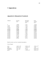
APPENDIX A: ATMOSPHERIC CONSTANTS......................................................................................................89
APPENDIX B: THEORETICAL BASIS OF CMARC.............................................................................................91
Table of symbols used ...............................................................................................................................91
subscripts:.................................................................................................................................................92
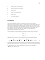
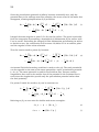
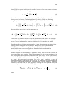
Panel Method............................................................................................................................................93
Computation of induced drag ...................................................................................................................97
Analysis of the boundary layer .................................................................................................................97
Offbody analysis ..................................................................................................................................... 104
APPENDIX C: TEACHERS' AND STUDENTS' GUIDE TO PSW.......................................................................... 107
Introduction ............................................................................................................................................ 107
Characteristics of the free stream in CMARC ........................................................................................ 107
It's no drag .............................................................................................................................................. 107
Initial exercises ....................................................................................................................................... 108
Using assembly and component controls................................................................................................ 109
Simple wing-body configurations ........................................................................................................... 109
Complex configurations .......................................................................................................................... 110
Modeling of small features...................................................................................................................... 110
Canards................................................................................................................................................... 111
Fillets and blends.................................................................................................................................... 111
Wing-wing intersections ......................................................................................................................... 111
Ground effect studies .............................................................................................................................. 112
Compressibility ....................................................................................................................................... 112
Internal flow problems............................................................................................................................ 112
Inlets and outlets..................................................................................................................................... 112
The Final Analysis .................................................................................................................................. 113
REFERENCES ................................................................................................................................................ 115
1
1. INTRODUCTION
Digital Wind Tunnel and CMARC
The basic analytical functions of DIGITAL WIND TUNNEL (DWT) are identical to
those of CMARC. Beyond the services provided by CMARC, however, DWT also
provides 2D analysis of airfoils and a simulation-based approach to predicting
static and dynamic longitudinal stability and static lateral-directional stability.
The initial setup dialogs are similar. CMARC and DWT use the same input file for
geometry definition and run management, and provide similar options for
overriding some run-control items. DWT, however, provides additional dialogs for
specific tasks related to stability and control, as well as an editor for inspecting
and modifying the input file.
Apart from its Windows interface components, CMARC is written in ANSI C and
may be compiled on a UNIX system without modification. Source code and
makefile are available at extra cost.
In the following general description, what goes for CMARC also goes for DWT,
unless otherwise stated.
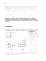
Array sizes and memory requirements
CMARC's data structures include a large square array whose dimension is the
number of panels in the model. Thus, if there are 1,500 panels in the model, there
are 1,500 x 1,500, or 2.25 million values in the array. Each value requires four
bytes of memory in single precision or eight in double, and so a 1,500-panel
model produces a main array, or "influence coefficient matrix," of nine megabytes
in single-precision operation.
Models too large for available RAM oblige CMARC to store the excess on the hard
drive. CMARC reports the amount of the array stored in RAM both as a number of
columns of the array and also as a percentage its total size.
2
CMARC can be run in either single or double precision. Double precision uses
about twice as much memory as single precision for a given model, and is
therefore likely to be much slower for large models, since it has to use the hard
disk for a larger proportion of its scratch file needs.
CMARC.DIM
A file called CMARC.DIM contains information that CMARC, DWT, and
POSTMARC use to fix the sizes of certain arrays. CMARC looks for it in several
locations, in this order:
1) the local directory (where the IN file is)
2) a directory pointed to by an environment variable, CMARC_INSTALL
3) the directory where CMARC.EXE is
Normally, a basic copy of CMARC.DIM should be in the CMARC.EXE directory.
Copies specific to certain projects can be kept with the project data files. If no
copy of the file is not found, CMARC reports at the start of the scrolling even log
that it is using "default cmarc.dim" and reverts to internal default values which
may not be adequate for the model being run but cannot be changed by the user.
Although it is possible to use a single CMARC.DIM for all analyses, some models
require much more array space than others. In general, however, memory
allocations -- the variables beginning with N -- should not be unnecessarily large,
although with the steady increase in the amount of RAM this is less and less of a
concern. The best way to ensure efficient use of memory is to put a copy of
CMARC.DIM, suitably dimensioned, into the home directory of models requiring
especially large amounts of memory (that is, large numbers of panels, multiple
wakes, etc). "Insufficient memory" errors may occur because some allocations
involve the product of two CMARC.DIM items. A number of arrays contain (4 *
NBPDIM * NPDIM) items.
For example, a wing with 30 spanwise panels, running an asymmetrical (ie twosided) case, will have a wake 60 columns wide, whereas the default version of
CMARC.DIM provides for a maximum of 50 columns. The result would be a
failure after the "Reading in Wake Information" message. The problem can be
corrected simply by changing the value of NWCDIM in CMARC.DIM. CMARC
provides explanatory messages for most memory-allocation failures involving
constants defined in CMARC.DIM.
PERCENTRAM is the percentage of available RAM that is used for storing all or
part of the large matrix. It is set at 80%, but in cases where part of the large
matrix is going to disk, execution time would be somewhat reduced if a larger
value were used. Too large a value, however, causes CMARC to run out of memory
for its other, smaller arrays. You can experiment to see how large the percentage
3
can be for a given model. As faster processors, larger hard disks and greater
supplies of RAM become common, concern over speed and model size becomes
less and less pressing.
IFOLDDIM is an internal loop-control constant. It is set at 100 to provide a speed
advantage. If you get an error message indicating that you ran out of memory in
lineq(), try setting IFOLDDIM to a smaller value, such as 20.
BLCFIT, SLPOLY and NCOVER are choices that can affect the speed and
convergence of the nonlinear loop. They do not affect the inviscid analysis or the
boundary-layer analysis when it is performed as a postprocessing operation.
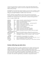
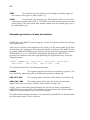
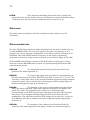
Here is a typical CMARC.DIM:
NSPDIM
8000 number of surface panels allowed (recalculated later)
NNPDIM
10
number of Neumann panels allowed
NPDIM
150 number of patches allowed
NBPDIM
300 number of basic points allowed -- not less than 50!
NWPDIM
5000 number of wake panels allowed
NWCDIM
200 number of columns or rows on each wake
NWDIM
10
number of wakes allowed
NSVDIM
10
number of scan volumes allowed
NSLPDIM
3000 number of points per off-body streamline
NONSLPDIM
3000 number of points per on-body streamline
NVELDIM
10
number of groups of panels on which non-zero normal
velocity is prescribed
PERCENTRAM 80
percent of available memory allocated to panel matrix
IFOLDDIM
100 looping parameter; change to 20 if out of memory in lineq()
SOLOPT
2
convergence criterion; use 1 for Pmarc, either 1 or 2 for
Cmarc
CPWARN
1000 threshold for "Unreasonable Cp" warnings
BLCFIT
1
curve fit method for boundary layer data; may be 1, 2, or 3
SLPOLY
3
order of polynomial used in curve fitting
NCOVER
10
number of streamlines to generate at a time when covering
body
Factors affecting execution time
CMARC execution times vary widely, depending on the number of panels in the
model being studied; the number of wake time steps requested; the number of
additional features, such as on- or off-body streamlines and velocity scan
volumes, that have been requested; the precision being used; and on other factors
more or less obscurely related to the geometry and paneling of the model.
Execution time is roughly proportional to the square of the number of panels in
the model. The choice of a grid density is therefore a compromise between
4
precision and speed. Typical CMARC models for wings contain between 1,000 and
3,000 panels; one side of a complete aircraft may easily require more than 4,000
panels. When asymmetric (eg sideslipping) flow conditions are being investigated,
or if the body itself is asymmetrical, a full model must be made and the execution
time will at least quadruple. Areas of particular interest can be more densely
paneled than the rest of a model. Sizes of two-sided models may be 7,000 to
10,000 panels or more. It should be noted, however, that the returns in precision
from increasingly dense paneling diminish rapidly, and at a certain point
disappear in the inherent approximation of a numerical simulation.
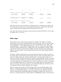
While it is running, CMARC provides an on-screen log of its activities, incremental
timings, and periodic estimates of time remaining. These estimates account only
for the time steps, not for streamlines, velocity scans, etc. A final run time is
reported at the end of execution. Typical run times for 3,000-panel models on
modern CPUs are on the order of half a minute. The total size of output files for a
single run is from one to five megabytes. The .FMT (ASCII) results file is two to
four times larger than the .BIN file and contains exactly the same information.
On modern computers with ample RAM, there is usually no difference in
processing time between single and double precision. Double precision is the
default. Models with numerically small dimensions, such as wings with a
normalized chord of 1.0, should always be analyzed in double precision.
Streamlines and velocity scans
CMARC's input deck provides for defining on- and off-body streamlines and scan
volumes of off-body points for pressure/velocity analysis. We do not recommend
placing these definitions in the input file, however, because it is inconvenient and
time-consuming to do so, and obliges you to re-run the full analysis every time
you want to change the streamline or scan selection.
POSTMARC will perform streamline and scan analysis interactively, using the
output from a single CMARC run. We suggest setting NBLIT to 1 in the input file,
providing representative density and Reynolds Number information on the
BLPARAM line (these may be changed in POSTMARC), and setting the numbers of
streamlines and scans in the input deck to zero.
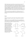
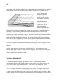
Inviscid vs viscous analysis
The basic equations used by CMARC to determine pressures and velocities over
the model surface do not take viscosity into account. Forces and moments are
5
reactions from accelerations induced by the model surface in the free stream. The
medium is assumed to be an ideal fluid that has no internal friction.
A fundamental limitation of such an analysis is that in the absence of viscosity
there is no drag other than induced drag. This may seem counterintuitive, since
the flow must be pushed aside to make way for the model, and this action would
seem to require some work. But an inviscid fluid is perfectly elastic. All energy
transferred to the free stream as the model pushes it aside returns to the model
as the free stream converges behind it. Obviously, an inviscid fluid is also by
definition free of internal shearing friction.
In the real world, where fluids are viscous, friction between a moving fluid and a
solid surface slows the flow near the surface, and the retardation is
communicated outward through the fluid. The retardation of flow adjacent to the
surface displaces the free stream outward, changing the magnitude and direction
of accelerations within it. The forces and moments experienced by the object or
model change as a result.
The magnitude of the outward shift of the free stream due to boundary layer
retardation is called the "displacement thickness" of the boundary layer. The
displacement thickness is the amount by which the solid surface would have to
be shifted outward in an inviscid flow to produce a loss of stream mass flow equal
to that due to viscous retardation within the boundary layer. Optionally, CMARC
can calculate the displacement thickness after each iteration of the solution and,
in effect, shift the centroid of each panel outward by that amount. The result is a
more refined solution that allows determining the pressure or "form" drag. The
choice of using this procedure, which increases execution time considerably and
reduces the stability of the numerical solution, is controlled by the NONLIN
parameter in the input file. The parameter is called NONLIN because it involves a
nonlinear mathematical procedure, and the more obvious name VISC was already
taken.
In the computational model, the characteristics of the viscous boundary layer are
determined by first computing streamline paths and then obtaining pressure
variations along them. An added flow component normal to the surface is used to
simulate the buildup of the displacement thickness. CMARC uses empiricallysupported two-dimensional methods to predict laminar transition, turbulent
separation, boundary-layer thickness, friction coefficient, and so on.
Although no inferences about pressure drag can be made from an inviscid
analysis, friction or "shearing" drag can be predicted with good accuracy by a
streamline analysis performed subsequently to an inviscid solution. Induced drag
of lifting surfaces is closely approximated by the Trefftz plane analysis once the
wake has stabilized, and also by the integration of surface pressures on lifting
surfaces. Thus, two of the three components of the total drag are obtainable with
an inviscid solution. Only the pressure drag component of the total drag (and a
small component of the induced drag) requires the full viscous analysis. Lift and
moment coefficients are more accurate, however, if the full viscous analysis is
performed.
6
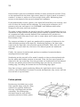
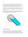
Solving the problem of turbulent reattachment
Under certain circumstances, flow near a surface stagnates in a rolling vortex
while flow farther away passes by smoothly, reattaching itself to the surface
downstream. This often happens, for example, at the base of a windshield.
Typically, CMARC predicts turbulent separation at these local stagnation points,
but has no ability to predict reattachment or failure to reattach. Thus, areas
downstream of a local stagnation point may be left without boundary layer
information, even though in reality the boundary layer would reattach and
continue to develop.
To circumvent the problem, you can identify groups of panels across which
boundary layer conditions are obtained by linear interpolation. Thus, the highpressure spike representing a local stagnation is replaced by a smooth transition,
and boundary-layer development along the streamline continues downstream. We
call this procedure a "jump"; panels across which the boundary layer should jump
are identified in the input file.
Base Drag
When flow separates, the pressure on downstream surfaces depends on the
surface geometry and also on Reynolds number. For example, the backside
pressure coefficient on a sphere is about -0.3 at moderate Reynolds numbers. The
same is true of a boat-tailed object like a bullet. On the other hand, pressures on
separated surfaces of wings at high angles of attack are less negative. CMARC
assumes a pressure coefficient of zero on separated surfaces, but POSTMARC
allows the user to select a different pressure coefficient.
7
2. Running CMARC and DWT
Environment
CMARC and DWT will run under any version of Windows, and on any modern
desktop or laptop computer.
Both programs make use of runtime libraries called CMSPDLL.DLL and
CMDPDLL.DLL. In addition, DWT uses a groups of five DLL files whose names
begin with GS. All these components should be present in the same folder as
CMARC.EXE and DIGIWT.EXE. POSTMARC makes use of them as well. Normally,
the install program takes care of the proper placement of files.
CMARC creates scratch files with names of the form Xnnn.TMP where nnn is a
sequential number. These are erased on normal exit. These files are normally
placed in the same folder as the input file, but you can force them to be placed
elsewhere by using an environment setting of the form tmp=c:\temp.
If a run terminates abnormally, scratch files may not be erased. Leftover files,
which may take up a great deal of disk space, should be manually erased from
time to time, as necessary.
Input files should be kept in separate "project" folders to reduce clutter. Output
files for each analysis go to the same folder as the input file unless you specify a
different path in the output file name.
To suppress the legal agreement dialog that appears at the start of a program run,
set the environment variable PSW_AGREE_YES by going to the Windows Control
Panel, the System icon, the Advanced tab, and the Environment Variables button.
Running CMARC
After you provide an input file name, CMARC by default gives its output files the
same name but provides different extensions (the characters following the period).
The extensions used are .OUT for the geometry and aerodynamic data output file,
.BIN for the binary plot file, .FMT for the (optional) ASCII plot file, .PM for the file
8
containing data used by POSTMARC for streamline and velocity-scan generation,
and .ONB for the on-body streamline output file. If you wish, you can cause the
output files to have a different name than the input file.
Input file names may have any extension you like, but the extension .IN is
customary in the PSW community.
Run option overrides
Various parameters in the input file can be overridden during the setup of
CMARC or DWT, without having to modify the input file.
The parameter called LENRUN in the CMARC input file controls the domain of the
analysis. The default value is 4, indicating that a full analysis, including all wake
time steps, is to be performed. To accept this option, check No override. Other
options are:
Run geometry only
The model is paneled and an output file is created
containing only the geometry information. The run takes only a second or two
and allows inspection of the geometry in POSTMARC.
Run geometry and initial wake
The geometry and initial wake, if any, are
modeled. POSTMARC optionally displays the wake separation line or lines. If
initial wakes are specified (ie, INITIAL=1 and at least one downstream section is
defined), the wakes can be displayed with <F9> in POSTMARC.
Run geometry and stepped wake
The geometry is modeled and the wake is
convected downstream, allowing inspection of wake panel size and the
downstream travel resulting from time-stepping. Wake roll-up does not take
place.
AOA and yaw override
Angle of attack and yaw angles may be set. Note that yawed cases required a
fully-defined two-sided model, and in many cases wakes may have to be specially
defined or rigid to prevent intrusion of the wake into the model. It is necessary
both to enter a numerical value and to check the box to implement the override.
9
Precision
The analysis may be run in single or double precision. (“Precision” refers to the
number of significant digits used internally by the computer, not to the quality of
the final results.) Single precision is sufficient for most cases. Double precision
requires more memory space and as a result may make large models run more
slowly. Rarely, a model may fail to converge in single precision but converge
properly in double precision.
Time steps override
You can set the number of time steps and their duration. (Note that the “size” of
the time step is a length of time, not a physical dimension.) If VINF is 1.0, then
the size of a time step should be of the order of magnitude of the model’s mean
aerodynamic chord. Otherwise, it should be that length divided by VINF in
consistent units.
For example, a model with a M.A.C. of 30 inches might have a step size of 30 if
VINF=1.0, but a step size of .001 if VINF=3000.0.
Boundary layer separation criterion
In developing the boundary layer along a streamline, a numerical parameter is
used to detect turbulent separation. The default value of this parameter is 0.02.
CMARC, DWT and POSTMARC all allow changing this parameter.
The separation parameter is of limited generality. A value that results in a
realistic prediction of separation on a wing does not give a realistic prediction for
a body of revolution. It is not possible, therefore, to find a single value that allows
a satisfactory prediction of separation for a complete aircraft model. For a specific
isolated component such as a wing or an airship hull, however, it is possible to
control the onset and propagation of separation with the separation parameter.
For a wing of typical planform and airfoil section, a value in the vicinity of 0.07
yields a plausible-looking separation pattern.
In order to select the separation criterion (most conveniently done by repeatedly
coating the model with streamlines in POSTMARC), it is necessary to have some
kind of knowledge of the expected separation behavior. When a value has been
found that produces a suitable separation pattern, test conditions can be varied
10
to investigate, for example, the progression of the stall with increasing alpha, or
the value can be applied to a full nonlinear (viscous) analysis.
Other options
Save both .FMT and .BIN plot files
By default, CMARC saves only a binary
file of plotting data. To port data between different operating systems, however,
an ASCII file is required; it has the extension .FMT.
Continue despite failure to converge
Causes CMARC to ignore the iteration
limit (MAXIT). To raise the iteration limit but prevent endless iterations, use Set
iteration limit.
Echo input to .ECO file for debugging
Creates a file with an .ECO extension
to allow inspection of the geometry and other input data as read by CMARC.
Write POSTMARC data in ASCII format
Writes the .PM file in ASCII format to
allow porting it between computers with different operating systems.
Set iteration limit
Overrides the value of MAXIT in the input file.
Run on disk or # columns in RAM
You can instruct CMARC to use the
hard disk rather than RAM for the main coefficient matrix, or you can specify
the number of columns of the coefficient matrix to be stored in RAM. These
options are intended for fine-tuning system performance for large models. The
number entered should be the maximum number of panels that can run in
RAM, that is, the square root of 20% of the installed RAM for single-precision.
If the model size is smaller than that maximum, leave the field blank.
Skip ancillary analyses
Omits streamline and scan volume analyses defined
in the input file. Since these operations can be more conveniently performed by
POSTMARC, we do not recommend defining ancillary analyses in the input file
at all; but some older Pmarc-12 input files have them.
11
Saving and re-using the initial solution
Usually, the first time step of an analysis requires about twice as many iterations
to converge as subsequent steps do. The solution of the first time step may be
saved and re-used in subsequent analyses to reduce the number of iterations in
the first step. The time saving is significant for very large, slow-running models.
Each solution file takes up about 35 kb of disk space.
Interrupting the analysis
CMARC will run to completion unless it encounters an input file syntax error or a
mathematical anomaly due to faulty patch geometry, or it runs out of memory, or
the solver fails to converge within the number of iterations specified by MAXIT.
The value of MAXIT in the input file can be overridden from the command line.
CMARC can also be instructed to continue processing despite a failure to
converge, which is commonly due to a faulty geometry and, in particular, to a
faulty wake definition. While the default value of MAXIT is 200, there is no harm
in setting a higher value, such as 1,000, since it has no effect on execution time
except in the rare instance where the solver fails to converge.
Processing can also be interrupted by hitting the Abort button next to the Start
analysis button. Execution will be cleanly terminated as though the number of
time steps executed so far were the number requested.
Running CMARC from a command line
An executable 32-bit DOS version of CMARC, and ANSI C source code with
makefile for a UNIX compilation, are available on request. Lacking a graphic
interface, they rely instead on command-line switches to set parameter overrides.
The form of the command line is
cmarc [filename] [switches]
Switches consist of a letter which in some cases is followed by an equals sign (=)
and then a number or a name. Under some circumstances, for instance when
running CMARC from a Windows DOS prompt or when executing it from a batch
file, the system may fail to recognize an equals sign and therefore fail to
implement the command-line override. In that case, replace the equals sign with a
colon (eg -a:5.0).
12
The letter-only switches are:
-b
Causes CMARC to save both the ASCII plot fine (.FMT) and the binary
plot file (.BIN), regardless of the setting of LPLTYP.
-g
Runs geometry only and then exits. This option is used for rapid testing
while creating the input file. Equivalent to LENRUN=2.
-w
Runs geometry and initial wake and then exits. Equivalent to
LENRUN=3.
-gw
Runs geometry and all wake steps and then exits. Equivalent to
LENRUN=4.
Continues analysis despite failure to converge in MAXIT iterations of the
-c
solver.
-f
Converts existing .BIN file to .FMT file. No analysis is performed. The
filename given need not include the .BIN extension.
-pa
Causes the .PM file to be saved in ASCII rather than binary format.
-e
Causes CMARC to echo input, line by line, to a file with the extension
.ECO.
-inv
-v
Performs an inviscid analysis even though NONLIN=1 in the input file.
Performs a viscous analysis even though NONLIN=0 in the input file, but
only if all of the values in BINP14 are present.
-am
Runs added-mass calculation only.
-sa
Skips ancillary analyses (eg streamlines, velocity scans).
-ss
Saves the solution from the initial time step for later use as a first guess.
Switches followed by a numerical parameter:
-a=
Sets the angle of attack to a value other than the one in the input file.
-y=
Sets the yaw angle to a value other than the one in the input file.
-s=
file.
Sets the number of time steps to a different value than that in the input
13
-t=
Sets the duration of the time step to a different value than that in the
input file.
-i=
Sets the maximum number of iterations for convergence (MAXIT).
-r=
Sets the number of columns of the main coefficient matrix that CMARC
should try to store in RAM.
-o=
Gives the output files a root name different from that of the input file.
-us=
Optional file name for initial time step stored with -ss.
-bl=
Sets criterion for boundary layer separation
14
15
3. 3D flow analysis in Digital Wind Tunnel and
CMARC
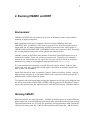
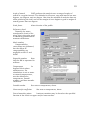
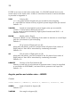
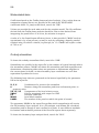
Setting parameters
The analysis of a 3D model in DWT is
similar to that in CMARC. Pick an
input file, then (in DWT) select
Analysis > CMARC
Set up the case using the various
options and “overrides” provided in
the dialog.
At the top of the form are the input file
name and, below it, the root name
which will be used to create output
files differentiated by their extensions.
These are the same by default, but
you can choose a different root name
if you wish.
The setup form for CMARC is similar,
though some items are in different
locations. CMARC provides the
additional option of setting up batch
operations for subsequent processing
(see below).
Running the analysis
Click on Start Analysis. The progress listing scrolls by in the window below,
while a progress window gives a continuous display of time remaining to the
estimated completion of time stepping.
16
To abort, click the Abort button to the right of the Start button. In order to
maximize execution speed, DWT checks comparatively seldom for user
messages, and so there may be a delay between the giving of the abort
command and the actual halting of the program.
Unlike Pmarc-12, CMARC and DWT always come to a programmed termination;
that is, the time step currently under execution ends cleanly with the present
iteration, and the usual files are created. It is therefore possible to examine the
results of an interrupted run up to the time step in which the interruption
occurred.
Batch processing
In CMARC (but not in DWT) setups can be stored for multiple analyses and
executed either immediately or at a future time, for example during the night.
Set up an analysis in the normal way. Then, rather than press the Start
Analysis button, press the Add button in the Multiple Analyses area at the
lower right corner of the CMARC display. You can repeat this step as often as
you like for the same or different input files, output file names, and overrides.
After compiling the list of analyses to be performed, you can set a time and
date. By default, these are initialized at program startup, and so if you do not
change their values the batch process will begin immediately.
Hit Submit to activate the batch file. CMARC will immediately shrink itself into
an icon on the status line. If you have set a future time and date for execution
of the batch process, a wristwatch icon appears. To restore the CMARC screen,
click on the status bar icon.
To remove an analysis from the list, highlight the line and press Remove.
Batch lists may be saved (Save) and retrieved (Load). The file extension is .CCL
(Cmarc Command List). Setup information from the batch list can be loaded
into the analysis form by double-clicking on the selected line in the list window.
CCL files are text files that can be manually edited, but it's safer to delete and
re-enter a case definition in Cmarc than to use an external editor to modify the
file.
If you attempt to quit CMARC while a batch is pending, a warning message
appears to verify that you intend to discard the batch process.
17
4. Digital Wind Tunnel: 2D profile analysis
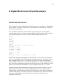
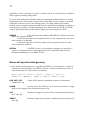
Airfoil data file format
The coordinates of the airfoil to be analyzed must be in AeroLogic’s .SD (Section
Data) format. (A utility, CVTSD.EXE, is provided for converting pre-1998 .SD
files to the new format.)
The .SD format is flexible and extensible, and allows users to incorporate
various kinds of data. Programs reading the files take from them only the data
they need, and ignore the rest. A typical .SD file might look like this:
@name
An airfoil
@crd
1.000000
@tcrat
0.120000
@rem
The thickness ratio is used by Loftsman.
@coords
1.000000 0.002000
0.997069 0.002688
0.988310 0.004766
...
1.000000 -0.002000
@end
modified 5/10/99 to incorporate this remark
Labels describing upcoming data are preceded by @. If a label is encountered
but not recognized, all the following lines are ignored until a new label is read
and recognized. After the @end label no more lines are read, but additional
material may be placed in the file for the reference of a human reader. The user
may also insert comments anywhere in the file (but not in the middle of a list of
items, such as airfoil coordinates), by preceding them with an @rem label.
Labels and their associated data may appear in any order in the file, but the
points represented by the coordinate list should start at the upper surface
trailing edge, proceed forward around the leading edge, and return to the lower
surface trailing edge. The listing need not be closed; that is, when the trailing
edge has a finite thickness the final point in the listing should not be a
repetition of the first.
18
When LOFTSMAN creates an SD file, the chord line is the longest line that can
be drawn from the center of the trailing edge (midpoint between upper and
lower surface trailing edge points) to another given point on the airfoil.
Coordinates are normalized for a chord length of 1.0. The airfoil is rotated so
that the chord line is always horizontal. If points are redistributed it is possible
for a point on the airfoil to have a station less than zero, and it is possible for a
trailing edge point (normally the upper surface point of an airfoil with finite
trailing edge thickness and a cambered trailing edge) to have a station slightly
greater than 1.0. Y coordinates are measured at a right angle to the chord line.
Airfoil coordinates usually have a full cosine distribution, with points closest
together at the leading and trailing edges. The analysis works best with this
arrangement, but neither LOFTSMAN nor DWT absolutely requires it. Although
LOFTSMAN puts no restriction on the number of points defining an airfoil,
DWT's 2D analysis is limited to 65 points per surface.
Loading an SD file
The file is selected and opened in the usual way, and appears in the edit
window. If you alter the file, you must save it before running the analysis.
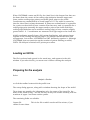
Preparing for the analysis
Select
Analysis > Section
or click the toolbar button with the profile icon.
The setup dialog appears, along with a window showing the shape of the airfoil.
Three items are provides for information only: the name of the input file, the
name of the airfoil (if any – the SD file may or may not contain a name), and the
numbers of upper- and lower-surface points.
The remaining fields are editable.
Output file
This is the file to which results will be written, if you
choose to save them.
19
Angle of attack
DWT performs the analysis over a range of angles of
attack at a regular interval. The defaults for the start, stop and interval are zero
degrees, ten degrees, and one degree. Note that the method of analysis does not
allow predicting the stall, and so the margin of error begins to grow at angles of
attack greater that ten degrees.
Scale factor
Alters the size of the profile.
Reference chord
Normally the mean
aerodynamic chord of the
wing, this is the value used
in obtaining dimensionless
moment coefficients.
Mach number
Compressibility
corrections are performed,
but the effects of
compressibility are
negligible at M=0.5 and
below.
Reynolds number
Note
that the RN is expressed in
millions.
Temperature
In
degrees Kelvin above
absolute zero. For
simulations in air or water
at normal temperatures,
use the defaults for
temperature, Prandtl
number, and heat transfer
coefficient.
Prandtl number
See note on temperature, above.
Heat transfer coefficient
See note on temperature, above.
Forced transition points
Laminar transition may be forced at the specified
fraction of the chord on upper and/or lower surface.
20
Performing the analysis
Click on Update section calculation. DWT analyzes the section at the specified
series of angles of attack, and results scroll by in the window. After the analysis
is completed, you can scroll back through the results. To display the chordwise
pressure distribution at various angles of attack, click on Previous alpha and
Next alpha.
DWT displays graphs for pressure distribution, lift coefficient, drag coefficient
(against both alpha and lift coefficient), and pitching moment about the
quarter-chord point.
21
5. Digital Wind Tunnel: Stability analysis
Method
DWT uses multiple CMARC analyses to calculate the derivatives that define
longitudinal and directional stability and roll rate. Certain geometry parameters
are varied between runs: elevator deflection with angle of attack (alpha) for
longitudinal stability, rudder deflection with yaw angle (beta) for directional
stability, and aileron deflections for roll rate.
For stick-fixed cases, control-surface deflection is varied to obtain the trimmed
condition, and the moment derivatives are obtained with the control surface fixed
at that deflection. For stick-free cases, the control surface deflection is varied at
each angle of attack or yaw angle to zero out the control surface load.
In all stability and roll rate calculations, multiple CMARC runs are used to
bracket solutions. DWT analyses therefore tend to take a long time and to
monopolize CPU resources. You can control how often DWT checks the operating
system for pending user commands by setting DWT’s priority to a lower or higher
level with a slider control in the main setup dialog.
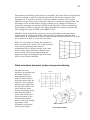
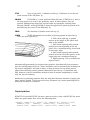
Simulating control surface movement
DWT simulates control surface deflections by rotating the surface normals of
panels about axes parallel to the surface hinge line, without moving the panel
centroids. This technique has been shown to be accurate up to approximately 15
degrees of deflection. It allows you to deflect control surfaces without having to
modify the paneling, which would be a time-consuming task. POSTMARC
provides a procedure for identifying the panels to be tilted and writing out the
required &BINP11A card for the input file. Once moveable surfaces have been
identified in the input file, they can be displayed by POSTMARC as well.
22
Aircraft properties
Load a CMARC input file and select
Analysis > Stability
The stability dialog box appears. In its upper left hand corner are a number of
fields for entering the physical properties of the aircraft.
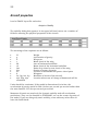
The meanings of the captions are as follows:
„
„
„
„
„
„
„
„
„
„
„
„
W
g
S
c
Sh
ch
lam
Xcg
Xt
b
Ixx, Iyy, Izz, Ixy
e@x, e@y, e@z
calculated
Weight
Acceleration of gravity
Wing area
Mean chord of the wing
Area of horizontal stabilizer
Mean chord of the horizontal stabilizer
Ratio of tip chord to root chord of the wing
Station of center of gravity
Location of horizontal tail quarter chord point
Wingspan
Moments of inertia of the aircraft.
Location where rate of change of downwash will be
Units should be consistent. If the model is dimensioned in inches, the
acceleration of gravity would be 386.4 inches per second per second rather than
the more familiar 32.2 feet per second per second.
Moments of inertia are used only for dynamic stability and roll acceleration
predictions. They can be obtained in POSTMARC, as can the center of gravity of
the model. If you are doing only static stability, enter arbitrary values here or
leave the fields blank.
23
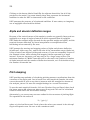
Saving and retrieving aircraft data
Once you have entered the physical properties for the aircraft, they can be saved
and recovered for subsequent runs. The file in which they are saved has the root
name plus the extension .CML, and it retains a record of each stability analysis
associated with a given .IN file name. Each record is identified by the time and
date of its creation. CML files are managed in the area headed File Management at
the lower right hand corner of the stability dialog.
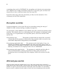
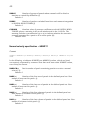
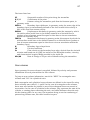
If the Auto save box is
checked, records are saved
automatically each time a
calculation is performed,
but you can also force a
save at any time by clicking
on the Save data button.
To re-load data entered
earlier and saved in the
CML file, click on the button
marked List stability runs, select a date and time, and click on Load Data. To
delete data for a certain run, select that run and click on Delete Data.
To load data from a CML file having a name different from the current input file,
click Import Data. Select the file name and then proceed as above.
Flight conditions
At the upper right corner of the main form, enter the true airspeed and the
density of the medium. Remember to keep units consistent; if the model is
dimensioned in inches, speed should be expressed in inches per second.
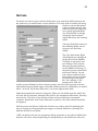
Identifying the stabilizer
Click on the button labeled Pitch in the Stability Modes area to bring up the setup
dialog for pitch stability.
24
Clicking on the button labeled Load fills the adjacent box with a list of all the
patches on the model. You must identify those that represent the horizontal
stabilizer in order for DWT to determine its lift coefficient.
DWT assumes the presence of a horizontal stabilizer. If none exists, an imaginary
one of negligible size should be defined.
Alpha and elevator deflection ranges
Because of the inviscid nature of the analysis, results are generally linear and are
applicable to a range of angles of attack in which separated flow is negligible.
DWT finds the trimmed angle of attack for the specified weight and speed, and the
required elevator deflection, by linear interpolation or extrapolation from
bracketing values entered by the user.
DWT prompts for starting and stopping values of alpha and elevator deflection
(Alpha start, Alpha stop, etc), and for the size of the intermediate steps (Alpha inc).
A step of one or two degrees yields good accuracy. If you are reasonably certain of
the trimmed values, enter starting and stopping values separated by a small
interval. If you are uncertain, you may wish to try a larger range at first. The
minimum number of CMARC runs that will be executed is the product of number
of alpha intervals and the number of deflection intervals, so it is desirable to keep
the number of intervals low.
Pitch damping
DWT provides two methods of calculating pitching moment contributions from the
curvature of the flight path. One is based on a semi-empirical formula; the other
curves the model in such a way that it interacts with the straight free stream of
the analysis just as if it were the straight fuselage in a curved free stream.
To use the semi-empirical formula, click on Calculate Cmq and Cmad, then check
the boxes next to the values you want to use (if any) and click on Use calculated
values to make DWT use the checked value(s).
Alternatively, you can set any non-zero radius for the curvature of pitching flight.
The equation for the radius is
V2 / [ g(n-1) ]
where n is the load factor and V and g have the values you entered in the Aircraft
Physical Properties area. Be sure to use consistent units.
25
DWT will automatically insert the proper value for a 2G pullup if you press that
button.
Elevator tilt
In order to simulate elevator deflection, you will have listed on the &BINP11A line
in the input file the groups of panels that represent the moveable surface. In the
field captioned Ele tilt, enter the ordinal positions of the elevator-related entries on
that line. For example, if the line starts with two rudder entries followed by four
elevator entries, you would enter 3 4 5 6 for Ele tilt. Do not enter patch numbers.
Alpha and elevator setting for longitudinal trim
To obtain the angle of attack and the elevator position required for trim at the
current weight, speed, and CG position, click only Calculate Trimmed Condition.
Close the dialog, go to the Run management section at the bottom of the form, and
click Run CMARC Analyses. Skip Ancillary Analyses and Save and Use Initial
Solutions should both be checked. Normally, single precision is sufficient, and
coefficients are referred to body axes.
DWT runs as many alphas and deflections as you have specified, and interpolates
or extrapolates the angle of attack and elevator deflection at which the lift is equal
to the weight and the pitching moment is zero. Results are placed in the fields
captioned Base Alpha and Elev Def.
Static longitudinal stability
To obtain longitudinal stability derivatives and the location of the neutral point,
check Stability derivatives. DWT provides default values of one degree for the
alpha and deflection increments; this should be satisfactory, but you can change
them if you wish. To obtain the neutral point, DWT must obtain the derivative of
Cm versus alpha at two different CG locations; the distance between them is dX.
The default value is 0.50; it can be changed by the user if it is not appropriate to
the model size and the units being used, but since the calculation is linear the
size of dX is actually of little importance.
26
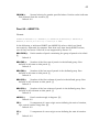
To obtain the rate of
change of moment
coefficient with elevator
deflection, check
Include Elevator.
If you have checked
Calculate Trimmed
Condition, DWT obtains
the trimmed values for
alpha and elevator
deflection before
performing the final
analysis and
interpolation; therefore
at least eight CMARC
runs take place.
If none of the options is checked, no longitudinal analysis is performed, but the
other data that you have entered are retained.
Performing the analysis
When you have finished setting up the conditions for the longitudinal analysis,
close the Pitch Stability dialog.
In the Execution area, Skip Ancillary Analyses, Save and Use Initial Solutions,
Single Precision, and Body Axes should normally be checked. To execute the
analysis, click on Run Cmarc Analyses.
The progress of both individual CMARC runs and the complete analysis is
reported graphically. In addition, continual reports on the status of each analysis
are provided in the scrolling status window. CMARC runs are separated by an
interval of about 10 seconds, during which memory cleanup is performed in order
to ensure that sufficient space will be available for the next run.
To stop an analysis, click on Abort. There may be an appreciable delay before
processing actually stops, because DWT checks for user commands at variable
intervals. The frequency of checks can be increased or decreased by the Priority
control in the main dialog.
27
Results of the longitudinal analysis
The results of the CMARC runs are displayed on the Pitch Stability dialog. The
meanings of the captions are as follows; all angular measurements are in radians.
CL
Lift coefficient for the complete aircraft based on wing area
CD
Coefficient of drag. Note that this value is not correctly
calculated by inviscid panel methods, and must be estimated and entered
by the user.
Cm
Pitching moment coefficient.
Cla
Rate of change of CL with respect to alpha.
Cda
Rate of change of CD with respect to alpha.
Cma
Rate of change of Cm with respect to alpha.
Cmq
Cm due to flight path curvature.
Cmad
Rate of change of Cm with respect to rate of change of alpha.
Clah
Lift curve slope of the horizontal surface.
de/da
Rate of change of downwash angle with respect to alpha at
the user-specified point
Cld
Rate of change of CL with respect to elevator deflection. This
value is only displayed; it is not currently used in any calculations.
Cmd
Rate of change of Cm with respect to elevator deflection. This
value is only displayed; it is not currently used in any calculations.
N(eutral) P(oint)
CG location where dCm/dCl = 0.
dCm/dCl
Rate of change of moment coefficient with respect to rate of
change of lift coefficient.
Dynamic longitudinal stability
Several steps must be taken prior to solving the quartic equation for dynamic
stability.
First, click on the button marked Cmq,Cmad. The appropriate values are inserted
into the Pitch Stability form; up to now, they have been zero. These values are
loaded manually to emphasize the fact that, for technical reasons, they are arrived
at by a separate mathematical method, and are not derived directly from the
CMARC output.
Second, enter a reasonable estimate of the parasite drag coefficient in the Cd field.
This step is necessary because an inviscid method such as CMARC’s cannot
determine parasite drag. Friction drag can be obtained from POSTMARC,
however, and augmented as necessary to account for flow separation, surface
roughness, cooling drag, etc.
28
Third, if you have not already done so, enter the moment of inertia about the
pitch axis (Iyy).
Fourth, click on Load Coefs. (Note that there are two buttons with this caption,
one in the Pitch Stability dialog and one in the Yaw Stability box.)
To solve, click on Dynamics. A new dialog appears.
DWT populates the matrices. The dynamic solution of the system matrices makes
use of a quartic equation. The Solve Quartic button solves the quartic for the four
roots, which may be real or complex. If complex, the roots will appear as complex
conjugates.
In the box headed Longitudinal Dynamics Evaluation, click on Calculate. DWT
returns the periods and damping coefficients of the short- and long-period
phugoids. Click on Longitudinal Evaluation for a verbal characterization of the
oscillatory modes and their damping, such as Aperiodic, convergent or Oscillatory,
divergent.
Static and dynamic directional stability
The procedure for analyzing directional stability is essentially similar to that used
for longitudinal stability. But yawed cases require attention to certain
characteristics of the model.
To begin with, the model must be fully defined on both sides of the plane of
symmetry. As a result of the number of panels being doubled, each CMARC
analysis takes about four times as long.
A wake must be defined for each vertical stabilizer, and the rudder portions must
be identified in the &BINP11A line in the input file.
Wakes for horizontal surfaces must be defined with the geometry of the yawed
case in mind. When CMARC time-steps a wake, sections are carried straight aft
by the free stream. Similarly, when you define a wake by copying the separation
line at a distance downstream and allowing CMARC to interpolate the intervening
sections, the copied sections are translated only along the X axis, ignoring the
attitude of the model in yaw. The user must ensure that lines emanating aft from
the wake separation line do not intrude into the model surface at any point when
the body is yawed. Difficulties can be minimized by using of very small angles of
yaw in the analysis, but in some cases it will be necessary to generate a special
rigid yawed wake (using LOFTSMAN) and to forego time-stepping, or to slightly
modify the geometry of the model in order to provide a converging wake
separation line.
29
Roll rate
To obtain roll rate for given aileron deflections, you must first define ailerons on
the model as you would other control surfaces. You may wish to modify the wing
mesh to ensure that panel
edges coincide exactly with
the ends and the hinge line,
but a good approximation
can be obtained by simply
using the nearest panel
edges offered by the existing
mesh.
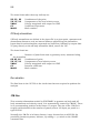
Click the Roll Rate button in
the Stability Modes row to
bring up the Roll Rate
dialog.
The Left Aileron and Right
Aileron fields are analogous
to the Ele Tilt and Rudder
Tilt fields in the pitch and
yaw dialogs. They require
that you list the positions,
in the &BINP11A listing, of
the panel groups associated
with each aileron. Do not
enter patch numbers here;
enter panel group positions
in the listing in the input
file. For example, if the
listing starts with two
rudder groups followed by four elevator groups, two left aileron groups and two
right aileron groups (both upper and lower surfaces must be included), you would
enter 7 8 in the Left Aileron field and 9 10 in the Right Aileron field.
Deflections should be entered in degrees. These are the deflections for which the
roll rate will be reported; normally they will be the maximum deflections, but they
need not be. The ratio of up-aileron to down-aileron deflection is assumed
constant. Remember that if one deflection is positive, the other should normally
be negative.
Roll Increment and Aileron Deflection Fraction are values used for obtaining the
rate of change of rolling moment per degree of aileron deflection. Normally the
defaults should be accepted.
DWT calculates roll rate by comparing rolling moments at two aileron deflections
and two roll rates, and extrapolating or interpolating to the deflections that you
30
specify. The numerical result is then modified according to an empirical
procedure derived from Hoerner, Fluid Dynamic Lift (p. 9-13, Fig. 2), and reported
both in degrees per second and as a wingtip helix angle in radians. An estimate of
rolling acceleration is also provided.
To obtain corrected values, enter the average aileron chord as a fraction of
average wing chord over the portion of the span occupied by ailerons, and click on
Calculate.
DWT’s corrected results agree closely with predictions obtained by other methods
(eg DATCOM, Roskam). The DWT approach is comparatively time-consuming, but
it has the advantage of being applicable to any configuration, whereas other
methods assume an airplane of more or less conventional arrangement.
31
6. The input file
General format
The input file consists of three major sections which contain general run control
information, body and wake geometry, and parameters for special services such
as velocity scans, streamlines, etc.
The format of the input file is nearly identical to the Fortran NAMELIST format
used by NASA's Pmarc-12 program. Each NAMELIST begins with an ampersand
(&) and ends with &END. Variable names are joined to values by equals signs.
Pmarc-12 requires that the first column in each new line be empty, and that the
starting ampersand be placed in the second column, but CMARC does not impose
this requirement. Position and spacing of entries within lines are not significant.
Line feeds are ignored, and an input line may extend over several physical lines. A
generic line might look like this:
&DATA
VAR1=2,
VAR2=0,
VAR3=0,
&END
The commas may be omitted.
When a line of entries refers to a previously defined item or items, it is skipped if
the number of items declared is zero. For instance, line &BINP10 (see below)
announces how many of various kinds of special modifications will be made to the
input. Lines &BINP11, &BINP11A, &BINP11B and &BINP12 provide detail about
these modifications. If a certain number in &BINP10 is zero, the corresponding
items in the subsequent lines are not read. Thus, you can leave values in the file,
but make them invisible by zeroing the controlling counter. For example, a wake
may be temporarily omitted from the analysis by setting IDWAK=0 for that wake.
Units
Any units of measure may be used, but they must be consistent throughout. For
example, if the body geometry is defined in inches, all speeds should be in inches
per second rather than feet per second or miles per hour. Likewise, VISC, the
kinematic viscosity, normally published in terms of feet, should be adjusted
(multiplied by 144 for inches, for example), and so on. Sea levels values for
32
kinematic viscosity in English units are approximately 0.00016 for feet and 0.023
for inches. See Appendix A for a listing of frequently used constants.
Some aspects of consistency of units are less obvious. Rates of rotation and
oscillation need to be adjusted to match the stated free stream velocity. For
example, in order to simulate a roll rate of 90 degrees per second in an airplane
traveling at 200 mph, while using a VINF of 1.0 in order to obtain output in
coefficient form, the roll rate must be divided by the speed in the appropriate
units. For a model sized in inches, PHIDOT would be 90 / (200 * 1.47 * 12) or
0.02551.
Similarly, if VSOUND (the speed of sound) is given its real value, then VINF must
also be a real value in order for the Mach display to have the proper units. If VINF
is 1.0, then the entry for VSOUND should be the reciprocal of the design flight
Mach number. For instance, an airplane travelling at 200 mph at 10,000 feet has
a flight Mach number of .273. If VINF is 1.0, VSOUND should be set at 1/0.273,
or 3.663, in order for the mapping of local Mach numbers to be meaningful.
Axes and rotations
A conventional coordinate system is used, with X representing the longitudinal
axis and increasing aft, Y the spanwise axis increasing to the starboard, and Z the
vertical axis increasing upward.
All rotations are performed in accordance with the right hand rule. That is, when
the right hand is held with the thumb pointing in a positive direction along an
axis of rotation, positive rotation about that axis is in the direction of curvature of
the fingers.
In the following, (R) indicates that a value is a real number, and may have a
decimal fraction component. (I) indicates an integer. (A) indicates an
alphanumeric, or text, entry.
The basic input page
The basic input page is the first section of the input file. In most cases, similar
models will be able to use similar basic input pages, with only a few numerical
changes. The most convenient way to create the basic input page is therefore to
edit an existing one.
33
Name and output instructions
Format:
Oneirodyne ZQ7
&BINP2 LSTINP=2 LSTOUT=0 LSTFRQ=0 LENRUN=0 LPLTYP=0 &END
&BINP3 LSTGEO=0 LSTNAB=0 LSTWAK=0 LSTCPV=0 &END
The first line contains a text title or description for the model. There are no
formatting restrictions, other than a limit of 80 characters, including blank
spaces.
The next two lines control the volume and formatting of output. The meanings of
variables are:
LSTINP
Input data print options (I):
0 = print all data except geometry
1 = print all data except detailed coordinates
2 = print all input data
Default: 2
LSTOUT
Output data print options (I):
0 = basic printout
1 = set additional options below
Default: 0
LSTFREQ
Printout frequency (I):
0 = Detailed panel data on last step, other data at each step
1 = All data at each step
N = Detailed data every N steps, other data at each step
Default: 1
LENRUN
Run scope [I]:
0 = Complete run
2 = Run geometry only and write to plot file
3 = Run geometry and wake initialization and write to plot file
4 = Run geometry and wake routines. Step through all time steps, but
perform no analysis. Geometry and wake data from all time steps are
written to plot file.
Default: 0
LPLTYP
Plot file type [I]:
0 = Unformatted plot file
1 = Formatted ASCII plot file
Default: 0
&BINP3 controls various print options. It may be omitted if LSTOUT is 0.
34
LSTGEO
Panel geometry printout [I]:
0 = Print option off
1 = Print all panel corners
2 = Print all panel corners and unit normal vectors
3 = Print all panel corners, unit normal vectors, and panel sets with
prescribed normal velocities
Default: 0
LSTNAB
Panel neighbor information printout [I]:
0 = Print option off
1 = Prints neighbor information for all panels
Default: 0
LSTWAK
Wake data printout options [I]:
0 = Print option off
1 = Prints wake-shedding information for each wake column
2 = Prints wake-shedding information for each wake column and wake line
geometry
3 = Prints wake-shedding information for each wake column and wake line
geometry, and wake panel doublet values
Default: 0
LSTCPV
Panel corner point analysis printout [I]:
0 = Print option off
1 = Prints panel corner point analysis results according to value selected in
LSTFRQ
Default: 0
Solver parameters: &BINP4
Format:
&BINP4 MAXIT=200 SOLRES=0.0005 NONLIN=0 &END
Two variables control the termination of the iterative process used to solve the
matrix. The first simply tells the program to stop iterating at a certain number,
whether a reasonable convergence has been achieved or not. This value may be
overridden from the command line with the -i= switch.
The second value is a measure of the degree of convergence desired. It represents
the size of the difference between two successive values of a solution parameter
expressed as a fraction of one of them, and as such is dimensionless and
independent of the units used. For good results, it should have a value of not less
35
than 1/100,000 of a characteristic dimension of the model. such as the wing
chord.
Either of two solution parameters may be used to measure convergence. Setting
SOLOPT to 1 in CMARC.DIM selects the parameter used by Pmarc-12. Setting
SOLOPT to 2 selects the parameter preferred by CMARC. Pmarc-12 ignores the
setting of SOLOPT. If no value is given, CMARC defaults to 2.
The NONLIN switch controls whether or not boundary layer analysis is
incorporated into the iterative solution. Nonlinear analysis significantly increases
processing time.
MAXIT
Default: 200
Number of solver iterations [I]
SOLRES
Convergence criterion for matrix solver [R]
Default: 0.0005
NB: The proper value for SOLRES is related to panel size, which is in turn related
to model dimensions such as CBAR and SSPAN. As a very rough guide, SOLRES
should be about 1/100,000th of CBAR.
NONLIN
Default: 0
Nonlinear solution incorporating BL analysis [I]
Time-step parameters -- &BINP5
Format:
&BINP5 NTSTPS=3 DTSTEP=20 &END
Cases involving computation of lift require that a wake be defined to prevent
violation of the Kutta condition at the trailing edges of lifting surfaces. The wake
may be defined in several ways (see below under Wake Geometry Section), some of
which involve allowing the wake shape to be modified by the computed pressure
distribution. In these cases, the solution is calculated repeatedly over a number of
"time steps," each time with a recalculated wake shape. The duration of a single
time step should typically be the length of time required for the model to travel
between one-half and one chord length.
The purpose of time-stepping a wake is to achieve a realistic simulation of the
downwash distribution. Often, computed pressure distributions are found to vary
negligibly from one time step to the next; in such cases time stepping is
unnecessary and the number of time steps can be small or zero. The usefulness of
time stepping in a given case can be estimated from the change in the integrated
lift coefficient from one time step to the next, or from the first step to the third or
36
fourth. In some instances, the wake calculation is unstable and additional time
steps give less rather than more accurate results.
NTSTPS
Number of wake time steps [I]
Default: 3
DTSTEP
Size of time step in seconds [R]
Default: 30
(The product of DTSTEP and VINF is the distance the model advances
between time steps. It should be roughly one half to one chord length.)
Symmetry and computation parameters -- &BINP6
Format:
&BINP6 RSYM=0.0 RGPR=0.0 RFF=5.0 RCORES=0.050 RCOREW=0.050 NABTOL=0.0001
&END
The symmetry parameters control reflection about two planes.
If RSYM has the default value of zero, the model is assumed to be symmetrical
about the XZ plane at BL0.0. The starboard half is modeled and CMARC assumes
the existence of a mirror-image port half.
If RSYM is 1.0, both sides of the model must be explicitly modeled. This must be
done either if the model itself is asymmetrical, or if the test conditions involve a
yaw rotation.
RGPR controls the ground plane. If RGPR is zero, no ground plane is modeled. If
RGPR is 1.0, a ground plane is placed at WL0.0. The effect is the same as if the
model were mirrored about the XY plane at WL0.0. If RGPR = -1.0, an infinite
Froude number approximation is used to model a free surface.
Four additional values allow tuning of the numerical procedure. These can be left
alone unless the user has a thorough understanding of their meaning.
NABTOL is a tolerance that is used to prevent averaging across panels that are
unusually close together but are not neighbors.
RSYM
Model symmetry [R]:
0.0 = body is symmetrical about Y=0
1.0 = body is asymmetrical or is symmetrical about a plane other than Y=0
Default: 0.0
37
RGPR
Ground plane [R]:
0.0 = no ground plane modeled at Z=0.0
1.0 = ground plane modeled at Z=0.0
Default: 0.0
RFF
Far field factor [R]. It is multiplied by a panel dimension to obtain
the far field radius for each panel. This value determines which of two methods
will be used to compute the influence of one panel upon another. The influence
of nearby panels is analyzed in greater detail. A higher value of RFF produces a
more accurate pressure distribution but slower execution.
Default: 5.0
RCORES
Surface panel core radius [R]. A nondimensional factor used when
computing velocities near a doublet panel edge. The value, which is multiplied
by the reference chord length (CBAR in &BINP9), controls the sensitivity of
velocity calculations to surface panel edges.
Default: 0.05
RCOREW
Wake panel core radius [R]. Similar to RCORES, but applied to
wake panels rather than surface panels.
Default: 0.05
NABTOL
Panel neighbor distance parameter [R].
Default: 0.0001
Free stream conditions -- &BINP7
Format:
&BINP7 VINF=1.0, VSOUND=3.782, IBCAM=0, AX=0.0, AZ=2000.0,
DENSITY=0.0002567, &END
The free stream velocity may be set to an actual value or to 1.0. If VINF is 1.0,
pressures and velocities emerge in coefficient form. Since dimensional pressures
and velocities can be obtained in POSTMARC, 1.0 is the most convenient and
versatile setting for VINF in CMARC.
If VINF is 1.0, VSOUND should be set to the reciprocal of the flight Mach number.
For example, if the actual flight speed is 240 mph and the speed of sound at the
intended altitude is 720 mph, then VSOUND should be set at 1/0.333, or 3.0.
CMARC does not make compressibility corrections; the only function of VSOUND
is to allow mapping of local Mach numbers. POSTMARC can perform
compressibility corrections on CMARC output.
38
If VINF is set to an actual value rather than 1.0, VSOUND should be set to its
actual value in the same units. A table of velocities of sound at various altitudes
is provided in Appendix A.
VINF
Velocity [R]:
1.0 = one global system length-unit per second for time-stepping
N = specified free-stream velocity in global system length-units per second
Default: 1.0
VSOUND
Speed of sound (global system length-units per second) [R]:
13392.0 = actual speed, inches per second
Or use speed of sound divided by flight speed of model with VINF = 1.0
Default: 13392.0
IBCAM
Model camber flag [I]
Instructs CMARC to use cambering of the model to simulate a curved flight
path for calculations of pitch damping..
Default: 0
AX
FS of center of flight path arc [R]
Along with AZ (below), sets the location in the XZ plane of the center of
flight path arc that will be simulated by cambering the model.
Default: 0.0
AZ
WL of center of flight path arc [R]
Along with AX (above), sets the location in the XY plane of the center of
flight path arc that will be simulated by cambering the model.
Default: 0.0
DENSITY
Density of the fluid medium [R]:
Density is used only in calculations of apparent mass. It may be specified
or overridden in POSTMARC, and need not be present in the input file.
Default: 1.0
Angular position and rotation rates -- &BINP8
Format:
&BINP8 ALDEG=0.0, YAWDEG=0.0, PHIDOT=0.0, THEDOT=0.0, PSIDOT=0.0, &END
ALDEG
Angle of attack in degrees [R]:
Default: 0.0
YAWDEG
Yaw angle in degrees [R]:
39
Yawed cases using time-stepping may encounter difficulty with the upwind
side of the wing wake intersecting the fuselage as it convects downstream.
See the section on wakes below for discussion of these situations.
Default: 0.0
PHIDOT
Rotation rate about global X axis, deg/sec [R]:
Default: 0.0
THEDOT
Rotation rate about global Y axis, deg/sec [R]:
Default: 0.0
PSIDOT
Rotation rate about global Z axis, deg/sec [R]:
Default: 0.0
Rotational oscillatory motion -- &BINP8A
Format:
&BINP8A PHIMAX=0.0, THEMAX=0.0, PSIMAX=0.0, WRX=0.0, WRY=0.0, WRZ=0.0,
&END
PHIMAX
Amplitude of oscillation about global X axis (deg) [R]:
Default: 0.0
THEMAX
Amplitude of oscillation about global Y axis (deg) [R]:
Default: 0.0
PSIMAX
Amplitude of oscillation about global Z axis (deg) [R]:
Default: 0.0
WRX
Rate of oscillation about global X axis (rad/sec) [R]:
Default: 0.0
WRY
Rate of oscillation about global Y axis (rad/sec) [R]:
Default: 0.0
WRZ
Rate of oscillation about global Z axis (rad/sec) [R]:
Default: 0.0
Note that one cycle of oscillation is equal to 2π for the purposes of defining the
rate. Thus, for an oscillation about the spanwise axis that requires 20 time steps
to complete, WRY would be 2π/20 or 0.314159.
40
Translational oscillatory motion -- &BINP8B
Format:
&BINP8B DXMAX=0.0, DYMAX=0.0, DZMAX=0.0, WTX=0.0, WTY=0.0, WTZ=0.000,
&END
DXMAX
Amplitude of translation about global X axis [R]:
Default: 0.0
DYMAX
Amplitude of translation about global Y axis [R]:
Default: 0.0
DZMAX
Amplitude of translation about global Z axis [R]:
Default: 0.0
WTX
Frequency of translation about global X axis [R]:
Default: 0.0
WTY
Frequency of translation about global Y axis [R]:
Default: 0.0
WTZ
Frequency of translation about global Z axis [R]:
Default: 0.0
Translational and rotational motions should be defined with respect to the value
of VINF and the base unit. For example, if VINF is 1.0 and the model's base unit
is the inch, a roll rate of 50 deg/sec at 150 feet per second actual forward speed
would correspond to a rotational rate of .0278 deg per inch of forward progress
(50 / [150 · 12] = 0.0278). The appropriate value for PHIDOT would therefore be
0.0278, not 50.
Rolling and yawing moments are normalized with respect to the semispan.
Reference dimensions -- &BINP9
Format:
&BINP9 CBAR=38.62 SREF=15194.0 SSPAN=210.0 RMPX=116.68 RMPY=0.00
RMPZ=-2.82 &END
CBAR
Reference chord for pitching moment [R]:
Set to M.A.C.
Default: 50.00
41
SREF
Reference area for force and moment coefficients [R]:
Set to wing area.
Default: 14400.0
SSPAN
Reference semispan for rolling and yawing moments [R]:
Default: 150.0
RPMX
X coordinate of moment reference point in global system [R]:
Default: 100.0
RPMY
Y coordinate of moment reference point in global system [R]:
Default: 0.0
RPMZ
Z coordinate of moment reference point in global system [R]:
Default: 0.0
Special options -- &BINP10
Format:
&BINP10 NORSET=2 NBCHGE=0 NCZONE=0 NCZPCH=0 CZDUB=0.0 VREF=0.0 NNROT=2
NPEXC=0 CPWARN=1000.0 &END
NORSET
Number of groups of panels with nonzero normal velocities (I)
Default: 0
NBCHGE
Number of panel neighbor information changes that are to be
made (I)
Default: 0
NCZONE
Problem type: 0 = external flow, 1 = internal flow [I]
Default: 0
NCZPCH
Number of the patch on which a doublet value will be specified for
internal flow modeling (I)
Default: 0
CZDUB
The doublet value set on the patch specified in NCZPCH for
internal flow modeling (R)
Default: 0.0
VREF
Reference velocity for computing Cp in internal flow. If left at 0.0,
VINF will be used (R)
Default: 0.0
42
NNROT
Number of groups of panels whose normals will be tilted to
simulate a control flap deflection (I)
Default: 0
NPEXC
Number of patches excluded from force and moment integration
in DIGITAL WIND TUNNEL [I]
Default: 0
CPWARN
Absolute value of pressure coefficient at which DIGITAL WIND
TUNNEL places a warning in the scroll window and in the .LOG file. The
warning includes a parenthetical (p) or (c) to indicate whether the excessive
pressure appeared on a panel or at a corner point. (R)
Default: 1000
Normal velocity specification -- &BINP11
Format:
&BINP11 NORPCH=1,22 NORF=0,0 NORL=0,0 NOCF=0,0 NOCL=0,0 VNORM=-0.53,0.95
&END
In the following, n indicates NORSET (see &BINP10) values, which are listed
successively, separated by commas. Note that each item needs NORSET values,
even if they are zeroes.
NORPCH(n)
Patch number of patch containing panels to receive a normal
velocity. (I)
Default: 0
NORF(n)
Number of the first row of panels in the defined panel set. Zero
means all rows on this patch. (I)
Default: 0
NORL(n)
Number of the last row of panels in the defined panel set. Zero
means all rows on this patch. (I)
Default: 0
NOCF(n)
Number of the first column of panels in the defined panel set.
Zero means all columns in this patch. [I]
Default: 0
NOCL(n)
Number of the last column of panels in the defined panel set. Zero
means all columns in this patch. [I]
Default: 0
43
VNORM(n)
Normal velocity for panels specified above. Positive value indicates
flow outward from the surface. [R]
Default: 0.0
Panel tilt -- &BINP11A
Format:
&BINP11A NROTPCH=17,17 NROTRF=1,31 NROTRL=8,38 NROTCF=2,2 NROTCL=8,8
ANGLE=0,0 VX=0.0,0.0 VY=1.0,1.0 VZ=0.0,0.0 &END
In the following, n indicates NNROT (see &BINP10) values, which are listed
successively, separated by commas. Note that each item needs NNROT values,
even if they are zeroes. Panel tilt is not supported by Pmarc-12.
NROTPCH(n) Patch number of patch containing the group of panels to be tilted.
[I]
Default: 0
NROTRF(n)
Number of the first row of panels in the defined group. Zero
defaults to all rows on this patch. [I]
Default: 0
NROTRL(n)
Number of the last row of panels in the defined group. Zero
defaults to all rows on this patch. [I]
Default: 0
NROTCF(n)
Number of the first column of panels in the defined group. Zero
defaults to all columns on this patch. [I]
Default: 0
NROTCL(n)
Number of the last column of panels in the defined group. Zero
defaults to all columns on this patch. [I]
Default: 0
ANGLE(n)
Panel rotation angle in degrees. [R]
Default: 0.0
VX(n)
X component of a zero-origin vector defining the axis of rotation,
eg a control surface hinge line. [R]
Default: 0.0
VY(n)
[R]
Y component of a zero-origin vector defining the axis of rotation.
Default: 0.0
44
VZ(n)
[R]
Z component of a zero-origin vector defining the axis of rotation.
Default: 0.0
Patch exclusion -- &BINP11B
Format:
&BINP11B NEXCLPCH=11,13 &END
Some models may include elements, similar to supports or stingers on wind
tunnel models, which are to be ignored during stability analyses by DIGITAL
WIND TUNNEL. Patches representing those elements may be enumerated here,
and the number of patches entered as NPEXC in BINP10. POSTMARC is unaware
of this parameter; you must exclude extraneous patches explicitly in POSTMARC.
Note -- in the following, n indicates NPEXC values (from BINP10), which are listed
successively, separated by commas.
NEXCLPCH(n)
Default: 0
Patches to be excluded in DWT stability analyses. [I]
Panel neighbor information change -- &BINP12
Format:
&BINP12 KPAN=368,378 KSIDE=2,2 NEWNAB=0,0 NEWSID=0,0 &END
CMARC computes velocities from doublet strength gradients between panels. In
some instances, such as along wake separation lines, potential differences can be
quite large and spurious velocities would be generated if gradients were computed
across these lines. CMARC automatically cuts neighbor relations along wake
separation lines and along the boundaries of assemblies. It is possible, but
seldom necessary, to make other modifications to the neighbor scheme.
Note -- in the following, n indicates NBCHGE (see &BINP10) values, which are
listed successively, separated by commas
KPAN(n)
Panel number requiring modified neighbor. [I]
Default: 0
KSIDE(n)
Side of KPAN(n) requiring modified neighbor. [I]
45
Default: 0
NEWNAB(n)
New neighbor panel adjacent to KPAN(n). [I]
Default: 0
NEWSID(n)
Side of NEWNAB(n) adjacent to KSIDE(n). If NEWNAB(n) is zero,
then NEWSID(n) should be set to -KSIDE(n) to cut the neighbor relationship
across KSIDE(n). [I]
Default: 0
Boundary layer calculation control -- &BINP13
Format:
&BINP13 NBLIT=1 NBLTRIPSEGS=3 &END
NBLIT
Perform or omit boundary layer calculations [I]
0 = no boundary layer computations performed by CMARC (the ability of
POSTMARC to perform boundary layer calculations is not affected)
1 = boundary layer calculations performed on specified streamlines. A BLPARAM
namelist must follow the onbody streamline input.
Default: 1
NBLTRIPSEGS
Number of segments of a boundary layer trip to force
laminar transition (I)
Default: 0
Nonlinear boundary layer calculation parameters -- &BINP14
Format:
&BINP14 MAXIT=15 NLTOL=0.1 CONTINUE=1 KEEP=0 RN=1000000.0
KVISC=0.00015639 MINCP=-15.0 MAXCP=15.0 MAXCOATS=50 NMON=1
MONITOR=212 NJUMP=3 &END
Nonlinear analysis is not supported by Pmarc-12. This line is read only if
NONLIN=1 (BINP4).
MAXIT
The maximum number of iterations allowed [I]
Default: 15
NLTOL
Convergence tolerance in percent [R]
46
Default: 0.1
CONTINUE
Allows the solution to continue if convergence is not found in
MAXIT iterations [I]
Default: 1
KEEP
Retains a POSTMARC-viewable .onb file for the final iteration
within each time step. KEEP=0 keeps only the last time step's .onb file [I]
Default: 0
RN
Reynolds number used for nonlinear iteration [R]
Default: 1e6
KVISC
Kinematic viscosity (R)
Default: 1.5639e-4
MINCP
Streamline calculations sometimes lead to wildly divergent
unrealistic values. Any streamline with Cp less than this value is discarded. (R)
Default: -15
MAXCP
Any streamline with Cp greater than this value is discarded. (R)
Default: 15
MAXCOATS
Limits the number of time the surface coating algorithm tries to
cover all panels. (I)
Default: 50
NMON
The number of monitor panels. Monitor panels are written to a
.MON file. The displacement thickness is written out. Typically this file is
brought into Excel in order to gauge the stability of the analysis by plotting the
behavior of the displacement thickness over time and iterations. (I)
Default: 0
MONITOR
The panels that are written out to the .MON file. (I)
Default: 0
NJUMP
The number of "jumped" panels. Jumped panels are listed in
BINP14A. (I)
Default: 0
Panel jumps -- &BINP14A
Format:
47
&BINP14A NJMPPCH=2,8,9 NJMPRF=17,11,10 NJMPRL=20,14,13 NJMPCF=12,1,1
NJMPCL=15,3,1 &END
Sudden steep pressure gradients along a streamline may trigger turbulent
separation. Once CMARC has detected turbulent separation in a streamline,
downstream calculation stops. In reality, however, flow may reattach downstream
from a separation bubble; this often happens on a windshield, where a small
bubble of stagnant high-pressure air forms at the base. Panels containing
pressure spikes may be "jumped." Pressures on jumped panels are obtained by
linear interpolation between panels before and after the jumped region.
In the following, n indicates NJUMP (BINP14) values, which are listed
successively, separated by commas. Note that each item needs NJUMP values,
even if they are zeroes. You may, however, leave lists in place if NJUMP is zero;
they are ignored.
Panel jumping is not supported by Pmarc-12.
NJMPPCH(n) Patch number of patch containing the panel(s) to be jumped. [I]
Default: 0
NJMPRF(n)
Number of the first row of panels in the defined group. Zero
defaults to all rows on this patch. [I]
Default: 0
NJMPRL(n)
Number of the last row of panels in the defined group. Zero
defaults to all rows on this patch. [I]
Default: 0
NJMPCF(n)
Number of the first column of panels in the defined group. Zero
defaults to all columns on this patch. [I]
Default: 0
NJMPCL(n)
Number of the last column of panels in the defined group. Zero
defaults to all columns on this patch. [I]
Default: 0
Boundary layer trips -- &BINP15
Format:
&BINP15 TOLER=0.001, XS=114.223694, 123.089111, 132.506561, YS=43.373150,
52.905602, 67.041115, ZS=-4.813857, -4.567827, -4.411704, XE=123.089111,
132.506561, 137.885895, YE=52.905602, 67.041115, 83.744118, ZE=-4.567827,
-4.411704, -4.161038, &END
48
NBLTRIPSEGS in BINP13, if non-zero, specifies a number of straight line
segments across which laminar transition will be forced in the streamline
analysis. Segments need not be contiguous. Because line segments are straight
but the model surface may be curved, a tolerance defines the distance from the
surface within which a trip segment will be recognized.
In the following, n indicates NBLTRIPSEGS (BINP13) values, which are listed
successively, separated by commas. Note that each item needs NBLTRIPSEGS
values. You may, however, leave previously defined lists in place if
NBLTRIPSEGS is changed to zero; they will be ignored.
TOLER Distance from the model surface within which the trip segments will be
recognized. [R]
Default: 0.001
XS(n)
X coordinates of the starting points of segments.
Default: 0
YS(n)
Y coordinates of the starting points of segments.
Default: 0
ZS(n)
Z coordinates of the starting points of segments.
Default: 0
XE(n)
X coordinates of the starting points of segments.
Default: 0
YE(n)
Y coordinates of the starting points of segments.
Default: 0
ZE(n)
Z coordinates of the starting points of segments.
Default: 0
49
Body geometry section
The geometry consists of bodies and wakes. A body is a three-dimensional solid,
while a wake is a zero-thickness sheet. The term "body" is often used here in a
general sense to mean an object in a fluid stream. In that case, it refers not only
to fuselages, nacelles, and so on, but also to lifting and stabilizing surfaces. When
a distinction is being made between procedures for bodies and those for lifting
surfaces, however, "body" has its usual meaning.
Bodies may be divided into as many as ten assemblies and ten components, each
with its own coordinate system. These are portions of the model surface for which
results will be listed separately in the output; for example, a wing might be
defined as a component in order to obtain loads on it separately from those on the
body. An assembly is usually a detached element, such as a slat or flap, but
certain patches, such as inlet diaphragms for air ducts, may be identified as
separate assemblies because CMARC does not average pressures across the
boundaries of an assembly. Every patch belongs to one assembly and one
component; components and assemblies may overlap.
The hierarchy of geometrical entities, starting from the bottom, is Point > Section
> Patch > Component > Assembly. Each level of the hierarchy from Section
upward provides facilities for translating and rotating the entities of which it is
composed, and translations and rotations are performed in bottom-up order.
Coordinate systems
The first entries in the geometry section define the coordinate systems for each of
the components and assemblies in the model. Each component or assembly has
an &ASEM1 or &COMP1 line defining the origin of its local coordinate system. If
the coordinate system of the item is to be rotated about an axis other than the Y
axis of the assembly coordinate system, an &ASEM2 or &COMP2 line is required
as well.
The format is as follows. In this example two assemblies, one of them with a
rotated coordinate system, and one unrotated component are identified. The
component's coordinate system is defined with reference to not to the global
system but to the assembly of which the component is a part.
&ASEM1
ASEMX=143.0000, ASEMY=25.0000, ASEMZ=-11.0000, ASCAL=1.0000,
ATHET=35.0, NODEA=0,
&END
50
&ASEM2
APXX=145.25, APYY=25.0000, APZZ=-10.1300,
AHXX=137.7700, AHYY=140.0, AHZZ=-8.563, &END
&ASEM1
ASEMX=135.0000, ASEMY=140.0000, ASEMZ=-8.0000,
ASCAL=1.0000, ATHET=0.0, NODEA=5
&END
&COMP1
COMPX=0.0000, COMPY=0.0000, COMPZ=0.0000,
CSCAL=1.0000, CTHET=0.0, NODEC=5,
&END
Note that the digits in labels such as &ASEM1, &COMP2, etc., refer to the type of
data, not to the order of the assemblies or components. Items are numbered as
CMARC reads them from the input file.
The meanings of the variables are as follows:
ASEMX, ASEMY, ASEMZ
coordinates. (R)
Origin of the assembly coordinate system in global
ASCAL
Scale. If ASCAL is negative, a rotation axis other
than the Y axis must be defined in ASEM2. (R)
ATHET
Rotation angle of the assembly in degrees, using the
right hand rule, eg downward deflection of a flap on a right wing is positive.
The rotation axis is the assembly Y axis unless ASCAL is negative. (R)
NODEA
If NODEA is 0, another assembly is defined after this
one. If NODEA is 5, this is the last assembly to be defined. (I)
APXX, APYY, APZZ
Starting point of the rotation axis in unscaled
assembly coordinates. (R)
AHXX, AHYY, AHZZ
Ending point of the rotation axis. (R)
Corresponding variables in a component block begin with C or COMP rather than
A or ASEM, but have the same meanings, except that component coordinates are
defined in terms of the coordinate system of the assembly to which the component
belongs, not the global coordinate system. At runtime, component rotations occur
first, then assembly rotations.
Patches
Each component or assembly is represented by a mesh of rectangular and,
occasionally, triangular panels. Panels are grouped in patches, which are
rectangular arrays of panels. The surface of a model is composed of one or more
patches. A patch may consist of a single panel or a single row or column.
51
CMARC numbers patches sequentially as it reads them from the input file. The
order in which patches appear in the file is generally unimportant, but it is
convenient to order patches from nose to tail along the starboard side of the body.
If desired, wing and other lifting surface patches may be defined first. Assemblies
that are in close proximity, such as a slotted flap and its associated wing, should
be kept close together in the input file. When a patch is mirrored across the plane
of symmetry (IPATSYM=1), CMARC increments the patch count by one
immediately after that patch is read. Thus, the first, second and third patches of a
model for which IPATSYM is equal to 1 become the first, third and fifth patches by
CMARC's reckoning, and the corresponding port-side patches are numbered 2, 4,
and 6.
In order to keep mirrored patches right-side-out, CMARC preserves the section
order but reverses the point order within each section. This fact becomes
significant when wake separation lines are being defined on the mirrored side of
the model.
Panels
The basic surface element is called a panel. Panels are defined as rectangles. A
panel that is triangular in shape is actually a rectangle with two corners that
coincide.
Panels may not have zero area. CMARC defines zero area as one millionth of a
square unit; thus, one square millimeter is the smallest permissible panel on a
model defined in meters. CMARC assigns the minimum area to all panels smaller
than the minimum and displays a "small panel" warning.
Normally, a panel has four
neighbors with each of which it
shares a side. It is impossible
to model a compound-curved
surface without distorting
panels, but it is desirable to
keep as many panels as nearly
rectangular as possible, and to
keep neighbors as nearly
aligned with one another as
possible. Adjoining panels
should also be of roughly
similar sizes. Finally, panel
warp should be minimized by
aligning patch boundaries with
local surface contours.
52
Ideally, the paneled body should be free of gaps between panels; that is, sections
at the adjoining edges of neighboring patches should consist of identical points.
CMARC will produce satisfactory results even if there are small mismatches
between patches, but it is preferable for the geometry to create a completely
closed object. It is permissible, however, and sometimes preferable, for openings
to exist at the far edges of the body, such as wingtips.
In order to approach the contour of the body as closely as possible, panels should
be small in areas of small radius of curvature, and may be larger in flatter areas.
More detailed information about areas of interest can be obtained by locally
increasing the mesh density. Accuracy generally increases with increasing mesh
density, but the returns diminish while the execution time increases
exponentially. A thousand panels are generally adequate for wing analysis.
Typical aircraft models may have 3,000 to 8,000 panels per side; it is difficult to
generalize because the required panel count depends on the surface complexity of
the design.
Patch definition
The numbers of panels in the rows and columns of the rectangular array forming
a patch is constant across the width and height of the patch. While patches are
considered for
convenience to be
rectangular in shape,
they can be distorted in
various ways. For
instance, a patch could
have the appearance of
a football, with a point
at each end.
Nevertheless, the row
and column counts
would be constant
throughout the patch.
Columns of panels in a
patch are defined by
"sections." In the case
of a streamline body,
sections are usually
vertical, or more or less
vertical, cross-sections.
In the case of a wing, sections usually correspond to imaginary ribs aligned with
the direction of flight. Sections are made up of "basic points," which are selected
surface points along the cross-section.
53
Two methods of defining basic points are available. The most direct and intuitively
natural is simply to specify the points that will be the corners of panels. The
alternative is to provide a number of points to define a contour, but to allow
CMARC to create basic points along the contour by curvilinear interpolation. The
advantage of the second method is that it allows you to change the density of
patches by changing one number (TNPS) in the input file. The two methods are
not mutually exclusive; you can start off by defining basic points yourself, and
later change the value of TNPS in the &SECT1 line.
CMARC’s point-interpolation function is most useful when analyzing simple
models such as a wing in isolation. When models involve many patches and
intersections, it is preferable to have all basic points explicitly defined in the input
file in order to be able to check and edit them.
When it is necessary to change the number of
rows or columns in a patch, one or more panels
in the more populous patch must be
triangulated out at the patch edge, and a new
patch, with a new point count, begun at the
same section. Each point representing the
degenerate edge of a triangular panel is listed
twice in the section definition.
Patch orientation and point, section and panel numbering
Patches have two
surfaces, an outside and
an inside. They are
distinguished by the
order in which section
and basic point data are
entered. If you imagine
placing your right hand
on the outer surface of a
patch with the point
counts increasing in the
direction the fingers
point, then the section
count increases in the
direction the thumb
points. This rule is valid
regardless of the
orientation of sections
and of panel edges.
54
Panels within a patch are numbered similarly to basic points and sections. Thus,
on the starboard side the lower right corner panel of a typical patch is number 1;
number 2 is above it; and so on to the to edge of the patch. Numbering then
returns to the bottom of the second column and continues.
If you inadvertently reverse a patch, your model will most likely not converge, and
even if it does the results will be nonsense. To check patch orientation, do a
geometry-only run and inspect it in POSTMARC with different solid colors
assigned to the inner and outer surfaces.
The order in which patches are placed in the file is usually unimportant, but it is
convenient to order patches in the same general manner as panels. Since the side
of a symmetrical body normally defined is the starboard side, patches are
generally arranged from nose to tail, and, in cases where one is above another,
from bottom to top.
The corners and sides of a patch are numbered for purposes of reference in the
wake-definition portion of the input file. Numbering begins at the lower right
corner and the right side, and proceeds counterclockwise. Thus, side one is the
right side, the top is side two, and so on. The sides of panels are numbered
similarly.
Finally, the corners of patches and panels are numbered counterclockwise,
starting with the lower right.
Numbering on the port side of the model is similar to that on the starboard side
but the point order within sections is reversed. Thus, the first row of panels is
adjacent to the top centerline. Port wing sections are numbered from the inboard
end out, but points proceed from the trailing edge over the top, around the
leading edge, and along the bottom back to the trailing edge again.
Note that as long as panel numbering follows the right-hand rule for outside
surfaces, the orientation of sections is actually unimportant; they can as well run
fore-and-aft as up-and-down.
Folded patches
Patches may be folded over so that
their opposite edges coincide. Wing
surfaces are typically defined in
this way, with edges two and four
coinciding. The trailing edge
thickness must be zero and the
spanwise positions of basic points
55
along the coincident edges must also coincide.
Folded patches are occasionally useful for bodies as well as wings. A tip tank, for
example, might be treated as a folded patch, with the wing joint being a gap in the
seam.
Care should be taken that vertical tail surfaces located on the median line of the
model be modeled according to the right-hand rule.
Sections
Patches are usually defined by groups of points along cross-sections normal to a
longitudinal or spanwise axis. This is a convenience, not a requirement, and panel
edges may deviate from neat vertical rows. Furthermore, body patches can be
defined by sections aligned with, rather than normal to, the longitudinal axis, and
wing panels can be defined by spanwise sections. Normally, however, the mesh of
panels constituting a patch is created by connecting corresponding points on
body and wing cross-sections lying in the YZ or XZ planes.
Patch description
Each patch description begins with an &PATCH1 line followed by a line
containing the patch name (which may be omitted, but the empty line must
remain). The name of the patch may begin in column 1. It is useful to include in
the name some patch information such as the sequential patch number and the
number of panels in the patch. The information can be obtained from the .OUT
file after a geometry-only run (-g switch on the command line).
The format of the &PATCH1 line is as follows:
&PATCH1 IREV=0, IDPAT=1, MAKE=0, KCOMP=1, KASS=1, IPATSYM=0,
IPATCOP=0, &END
WING (1, 280)
The meanings of variables are as follows:
IREV
Patch reversal flag. If IREV is 0, the patch is not reversed;
that is, the given point order is used. If IREV is -1, the inside/outside
orientation implied by the order of point and section entry is reversed. See the
discussion of duct flow below for some practical instances of patch reversal. (I)
56
IDPAT
Patch type. Three values are possible. 1 indicates a wing;
section force and moment data are generated. 2 indicates a body; no section
data are generated. 3 indicates a Neumann patch or vortex lattice sheet. (I)
MAKE
If MAKE is a positive integer n, CMARC automatically
generates a wingtip on side 3 of patch n. This is the normal arrangement with a
starboard wing. If MAKE is negative, the wingtip patch is generated on side 1 of
the patch (left wing). For all patches other than automatically generated tip
patches, MAKE should be 0. If MAKE is non-zero, a &PATCH2 line must follow
this line. [I]
KCOMP
The number of the component to which the patch belongs.
Zero defaults to 1. [I]
KASS
The number of the assembly to which the patch belongs.
Zero defaults to 1. [I]
IPATSYM
If IPATSYM is 1, another patch is generated, mirroring this
one about the XZ plane of symmetry. The mirror patch is numbered
immediately following this one. If no symmetrical copy is to be generated,
IPATSYM is zero. The section order of mirrored patches is the same as that of
their prototypes, but the point order within sections is reversed. (I)
IPATCOP
If IPATCOP is a positive integer n, then this patch is an
optionally translated, scaled and/or rotated copy of a previously defined patch
whose sequential number is n. A &PATCH3 line, defining the changes to the
copied patch, must follow the patch name line whenever the value of IPATCOP
is non-zero.
Automatic wingtip patch generation
To close the tip of a wing, provide a PATCH1 line in which MAKE has a non-zero
value, namely, the patch number of the wing panel of which this is the tip. A
&PATCH2 line immediately follows the &PATCH1 line. Note, again, that the 2 in
&PATCH2 refers to a type of patch definition, namely a wingtip patch, not to the
sequential order of patches.
A tip patch on edge 3 of patch 4 has the following appearance:
&PATCH1 IREV=0, IDPAT=1, MAKE=4, KCOMP=1, KASS=1, IPATSYM=0,
IPATCOP=0, &END
WINGTIP
&PATCH2 ITYP=1, TNODS=3, TNPS=3, TINTS=3, &END
57
ITYP
Type of tip patch. 1 indicates a flat tip. 2 indicates a circular arc
cross-section in the YZ plane. (I)
TNODS
If TNODS is 3, more patches follow this one. If TNODS is 5, this is
the last patch to be read in the geometry input. If others follow, they are
ignored. Misbehaving input files can be tested by repeatedly running them
through CMARC, moving TNODS=5 down through the file patch by patch until
encountering the cause of the difficulty. (I)
TNPS
The number of panels across the tip. (I)
TINTS
TINTS determines the method of spacing panels across the tip.
There are four options: [I]
0. Full cosine spacing, ie panels
narrow at the edges of the patch and
wide at the middle.
1. Half cosine spacing with narrow
panels near the beginning of the tip
patch. For a starboard wing, this would
be the lower edge.
2. Half cosine spacing with narrow
panels near the end of the patch, ie the
upper edge on a starboard wing tip.
3. Equal spacing. This is usually the
logical choice.
Automatically generated tip closures often produce unrealistically low pressures
near the trailing edge of the tip. These anomalies can be prevented by omitting the
tip closure altogether. No harm is done, so long as there are not other panels
(apart from the wing surface panels themselves) near the tip. Consultants may
find, however, that an inordinate amount of time is wasted explaining to clients
why the tips are missing.
Automatic tip paneling assumes that the wing has the same number of upper and
lower surface panels. If this is not the case, automatic tip closure paneling will be
distorted and may be unusable.
Copied patches
If IPATCOP in the &PATCH1 line has a non-zero value, then a &PATCH3 line must
follow the patch name line. It has the following form:
&PATCH3 PATX=52.00, PATY=1.765, PATZ=11.63, PSCAL= 1.0000,
PTHET=0.0000,
NODEP=0, PPXX=0.0000, PPYY=0.0000,
PPZZ=0.0000, PHXX=0.0000, PHYY=1.0000, PHZZ=0.0000 &END
58
The variables are as follows:
PATX, PATY, PATC
Translation vector for the copied patch relative to
the original patch whose sequential number is given by IPATCOP. The vector is
in global coordinates. (R)
PSCAL
Scale factor for this patch relative to the original patch. (R)
PTHET
Rotation angle in degrees of this patch relative to the
original patch. A non-null axis of rotation must be defined (see below). Rotation
follows the right hand rule. (R)
NODEP
If NODEP is 0, another patch definition follows this one. If
this is the last patch to be defined, NODEP must be 5. (I)
PPXX, PPYY, PPZZ
Starting point, in global coordinates, of the rotation
axis; this must be distinct from the end point even if PTHET is zero. (R)
PHXX, PHYY, PHZZ
End point of the rotation axis. (R)
Section format
Each section in a patch may take one of three forms: a list of basic points, a
NACA 4-digit airfoil, or a line of revolution. Each section may be defined in terms
of the global coordinate system, or alternatively in terms of its own local
coordinate system. Furthermore, the given points may be used as the corners of
panels, or they may be splined by CMARC and a different paneling arrangement
interpolated.
The most elementary situation, especially when formatted segments of a body are
being produced by LOFTSMAN, is a list of basic points to be used as panel
corners.
Each section begins with an &SECT1 line in the following format:
&SECT1 STX=0.0, STY=0.0, STZ=0.0, SCALE=1.0, ALF=0.0,
THETA=0.0, INMODE=4, TNODS=0, TNPS=0, TINTS=0, &END
STX, STY, STZ
coordinates. (R)
Origin of the section coordinate system in component
SCALE
Section scale. If SCALE is 0.0, the section becomes a single
point at the origin of the coordinate system. (R)
59
ALF
its Y axis. (R)
Rotation in degrees of the section coordinate system about
THETA
axis. (R)
Rotation angle of the section coordinate system about its Z
INMODE
May have the following values (I):
0. Copies the definition of the previous section.
1. The section is defined by Y, Z, dX coordinates. The X coordinate
defaults to 0.0 in the local coordinate system, but deviations can be entered in
dX.
2. The section is defined by X, Z, dY coordinates. The Y coordinate
defaults to 0.0 in the local coordinate system, but deviations can be entered in
dY.
3. The section is defined by X, Y, dZ coordinates. The Z coordinate
defaults to 0.0 in the local coordinate system, but deviations can be entered in
dZ.
4. The section is defined by X, Y, and Z coordinates. (This is the most
commonly used option.)
5. A NACA 4-digit airfoil section is automatically generated. A &SECT2
line must follow this one.
7. The section is defined by polar, ie rho, X, and theta coordinates. Rho
is measured perpendicular to the X axis. Theta is measured in degrees from the
positive (ie starboard) Y axis with rotation defined by the right hand rule.
All options except 0 and 5 must be followed by a listing of basic points
and a &BPNODE line (see below).
If the value of INMODE is negative, a body of revolution is generated. In
this case, the section definition is understood to be in the XZ plane. See
Automatic generation of a body of revolution below for further information.
TNODS
(I):
Defines section type. TNODS may have the following values
0. This is the first section or an intermediate section in the patch.
1. This is a break point on a patch. The slope is continuous into the next
portion of the patch.
2. This is a break point on a patch. The slope is discontinuous into the
next portion of the patch.
3. This is the last section in this patch.
5. This is the last section in the last patch in the geometry definition.
Any subsequent sections are ignored.
TNPS
If TNPS is zero, panel corners are defined by the basic
points lists given. If TNODS is 1 or 2 and TNPS is a positive integer, TNPS is
the number of panels that will be automatically inserted between this break
point and the previous break point, using curvilinear interpolation based on
the points you have supplied. If only the first and last sections of the patch are
supplied, interpolation is linear.
60
LOFTSMAN by default defines all sections in a patch explicitly. Input files can,
however, be manually edited to remove all but the first and last sections in ruled
patches and to insert interpolation instructions. This technique is useful for
debugging a file with a coarse mesh that executes rapidly, and then increasing the
mesh density for the final analysis.
TINTS
As in the &PATCH2 line, TINTS controls the type of spacing
for automatically interpolated panels. The possible values are 0 for full cosine
spacing, 1 for half cosine with smaller panels near the previous break, 2 for
half cosine with smaller panels near this break, and 3 for equal spacing. If
INMODE is 4, this is ignored.
Usually INMODE is 4 and TNPS is zero, and the &SECT1 line is followed by a list
of basic points. These are the points on the body surface that define the corners of
panels. Within a patch, all such lists must have the same length. If you want to
change to a different point count or spacing, you can change TNPS to the desired
point count and use TINTS to select the type of spacing.
Basic points on bodies are most usually listed from bottom to top; those on wings
are ordered from the trailing edge along the bottom to the leading edge, and then
back to the trailing edge over the top. But if need be, body section points may run
fore-aft, and wing section points may be arranged spanwise. There is one point to
a line, defined by three coordinates without delimiters other than one or more
spaces:
142.8305
142.8305
142.8305
142.8305
142.8305
142.8305
0.0000
4.9666
9.2749
12.5615
14.7977
15.6029
-15.6029
-14.7913
-12.5468
-9.2550
-4.9475
0.0000
Break points
Each basic points list ends with a &BPNODE line, which identifies a break point.
Break points may also be placed anywhere within a section to allow control of the
spacing of automatically generated panels. The format is typically as follows:
&BPNODE TNODE=3, TNPC=0, TINTC=0, &END
TNODE
If TNODE is zero, the preceding point is a first or
intermediate point. The rest of the &BPNODE line is ignored.
If TNODE is 1, the preceding point is a break point with a continuous
slope into the next region of the section.
61
If TNODE is 2, the slope into the next region is discontinuous.
A value of 3 indicates that the preceding point is the last one in this
section.
TNPC
Indicates the number of points to be automatically generated
between this break point and the preceding one. Zero indicates that no point
generation will take place, and instead the given basic points will be used as
panel corners. [I]
TINTC
Spacing of automatically generated points. The possible values
are 0 for full cosine spacing, 1 for half cosine with smaller panels near the
previous break, 2 for half cosine with smaller panels near this break, and 3 for
equal spacing. [I]
Note the analogy between TNODS-TNPS-TINTS and TNODE-TNPC-TINTC. The first
group refers to spacing of sections, the second to spacing of points (ie panel
corners) on sections.
Automatic airfoil generation
If INMODE is 5 in the &SECT1 line, a NACA 4-digit airfoil is automatically
generated. This option is chiefly useful for tail surfaces and for studying wing
characteristics when the airfoil type is not important. Automatically generated
airfoils look a little peculiar at non-zero angles of attack. It may be preferable to
avoid use of this option, and to rely on LOFTSMAN for airfoil sections instead.
A line of the following type must immediately follow the &SECT1 line:
&SECT2 RTC=0.13, RMC=0.2, RPC=0.4, IPLANE=2, TNPC=15, TINTC=0
&END
The variables are as follows:
RTC
Thickness/chord ratio. [R[
RMC
Maximum camber/chord ratio. [R]
RPC
[R]
Location of maximum camber as a fraction of the chord length.
IPLANE
The plane of the rib in the section coordinate system. 1 is the YZ
plane, 2 is the XZ plane (typical for wing ribs), and 3 is the XY (typical for
vertical fin ribs). [R]
62
TNPC
The number of panels between the leading and trailing edges of
the airfoil on the upper or lower surface. [I]
TINTC
As previously, the spacing type. The possible values are 0 for full
cosine spacing (the usual choice), 1 for half cosine with smaller panels near the
trailing edge, 2 for half cosine with smaller panels near the leading edge, and 3
for equal spacing. [I]
Automatic generation of a body of revolution
If INMODE in the &SECT1 line is negative, a body of revolution about an arbitrary
axis is generated.
Only one set of basic points appears in the patch; it is the axial profile of the body
of revolution. The spacing of circumferential panels is defined in the &SECT1 line
by setting TNPS and TINTS to the number of panels and the spacing type desired.
TNODS must be 3 or 5. A &SECT3 immediately following the &SECT1 line
provides the rotation vector and angle (following the right-hand rule). It has the
following format:
&SECT3 GAMMA=-180, GPX=0.0000, GPY=0.0000 GPZ=41.0000,
GHX=1.0000,
GHY= 0.0000, GHZ= 41.0000
&END
The variable names have the following meanings:
GAMMA
The rotation angle for the body of revolution, typically -180
for a half-body when the profile is defined with positive Z offsets. (R)
GPX, GPY, GPZ
The starting point of the axis of the body of revolution. (R)
GHX, GHY, GHZ
The ending point of the axis. For bodies of revolution
aligned with the free stream, only the value of GHX changes. (R)
Finally, one or more basic points defining the section are listed, separated by
&BPNODE lines as required. In the absence of interpolation instructions, panel
edges will be generated for each of the listed points.
The NASA documentation for Pmarc-12 states that the &SECT3 line should follow
the basic point input. This is incorrect.
63
Duct flow
CMARC will model flow through a duct. The duct may be fully defined or an inlet
and outlet may be provided and the internal cavity represented solely by
boundary surfaces with specified inlet and outlet velocities.
Flow through a duct with an inlet and/or outlet is not "internal" flow. CMARC
considers an internal flow to be one that is completely isolated from the outer
world, for instance a flow within a wind tunnel. Therefore internal flow does not
usually occur in the modeling of streamline bodies, and the variable NCZONE in
the &BINP10 line of the run control page is normally zero.
If the surface geometry of a duct is defined and patches are created using
LOFTSMAN, the patch reversal flap IREV (in the &PATCH1 line) must either be set
manually to –1, or the section or point order in the patch must be reversed with
LOFTSMAN’s patch-editing functions. LOFTSMAN itself does not distinguish
between internal and external surfaces when defining them.
When the outer-surface flow is of primary interest, the portion of the flow that
passes through an undefined cavity such as an engine compartment, radiator, jet
engine, etc., is usually dealt with by placing diaphragms across the duct at the
inlet and outlet. The location of these diaphragms is up to the user; for a jet
engine, for example, the inlet diaphragm may be placed at the engine face and the
outlet flush with the trailing edge of the duct. The inlet diaphragm should be
placed at least far enough inside the duct to reveal the stagnation behavior at the
inlet lip and the flow conditions within the duct entry. Stagnation is not an issue
with outlet flows, and so it is not necessary to recess the outlet diaphragm within
the duct. Diaphragms should, however, be normal to the flow direction.
Diaphragms usually consist of a single patch, one of whose edges is the perimeter
of the diaphragm. If points are listed in clockwise order (when seen from the front)
beginning at the bottom, the patch reversal flag of an inlet (ie forward-facing)
patch must be set to -1.
CMARC simulates flow through the duct by applying normal velocities to the
diaphragms. Velocities are listed as VNORM in line &BINP11 on the run control
page. To prevent averaging of velocities between the diaphragm and the
neighboring duct walls, assign the duct and the diaphragm to different
assemblies.
Normal velocities may be determined by consideration of the anticipated mass
flow, speed, and inlet or outlet area. The following values can be used as
guidelines:
Radiator or air-cooled engine inlet
Engine combustion air inlet
Jet engine inlets, low speed/high power
Exhausts, vents
0.2 - 0.8
0.7 - 0.9
1.0+
0.8
64
Jet exhaust (cruise)
1.2 - 1.3
Jet exhaust velocity ratios at cruise are approximately equal to the reciprocal of
the flight Mach number.
Normal velocities are positive when the flow direction is away from the surface.
Thus, inlet velocities are negative. To verify that normal velocity and the patch
reversal flag are properly set for a diaphragm, run CMARC and inspect the patch
velocities in the .OUT file. When flow is fore-to-aft, the value of VX should be
positive for all diaphragms.
Unlike VSAERO, CMARC will not model jet plumes or prop wakes successfully
because they involve a different total pressure from their surroundings. Outlet
pressures should be set at 1.0 for reliable modeling. Alternatively, the inside of
the duct can be fully defined as a surface and air allowed to flow all the way
through it. If one is desired, a wake may be constructed emanating from the
perimeter of a tailpipe, but in CMARC it will have little effect on the solution.
Internal flow
An internal flow is one in which panel normals face inward toward a closed cavity
that has no connection with or leakage to the outer world. The "inlet" and
"exhaust" surfaces of the cavity may be complete patches or groups of panels
within a patch. Usually, they are modeled as diaphragms. The external surface of
the cavity can be modeled in the normal way, and IREV then set at -1 for all of its
patches. To test the orientation of patches, run CMARC with the -g command line
switch and then examine the model in POSTMARC with different solid colors for
the positive and negative surfaces. When you hit <F8> (hidden line removal), the
outside of the entire model should appear with the solid coloring appropriate to a
negative surface.
To specify an internal flow case, NCZONE is set to 1. A flow rate is established by
defining an inflow velocity (VNORM) for either the inflow or the outflow patch. A
positive normal velocity would represent flow into the cavity. No normal velocity is
specified for the other diaphragm; instead, a constant doublet strength, and
therefore no tangential velocity, is constrained on that patch by setting NCZPCH
to the patch number of that patch in the BINP10 namelist, and CZDUB to 0.0.
CMARC automatically determines the normal velocity for that patch based on its
area and the conservation of mass.
If the model fails to converge, try modeling the NCZPCH patch without any
triangular panels. LOFTSMAN provides an option for paneling diaphragms
without using any triangular panels; it models the panel as a ring with a small
island in the center. In this case, the outer ring is specified as the NCZPCH patch,
and the small central area is simply treated as part of the wall.
65
Once the duct has been modeled, objects can be placed inside it as desired.
Because the Neumann boundary condition is imposed only at panel control
points, the shell of an internal-flow model may be subject to some leakage. This
can be minimized by increasing the paneling density of the cavity walls; by
increasing the far field factor (RFF in BINP6); or by adjusting the magnitude of the
free stream velocity vector to make it as close as possible to the average flow
velocity within the cavity.
66
Wake geometry section
Function of wakes
In order for a surface to produce lift, flow must be prevented from circulating
around the trailing edge. CMARC uses an imaginary membrane called a "wake" to
separate upper-surface from lower-surface flow. The wake may be thought of as
the "downwash sheet." If no wake is provided for a lifting surface, the pressure
distributions on it and on the rest of the model will be incorrect.
CMARC provides several options for dealing with the wake. It may be fully predefined, or it may be generated by CMARC from a separation line specified by the
user. It may be rigid or flexible. Finally, the number of time steps in wake
development, and their duration, may be defined. When VINF is 1.0, it is
convenient to set the time step roughly equal to the wing chord measured in the
default unit.
At first, INITIAL can be set to zero and the wing analyzed in isolation. CMARC can
be allowed to generate the wake for ten or twenty time steps to provide a sense of
its correct shape and position. The wake may then be predefined (INITIAL=1,
IFLXW=0) and iterated for three to five steps. If there is little or no change in
calculated values from one time step to the next, NSTEPS can be reduced to as
little as zero. In cases where there is a risk that a portion of a body might
penetrate a wake, such as a wing operating in the wake rollup of a canard
surface, the wake must not be time-stepped; NSTEPS should be zero.
Normally, a time-stepped wake is relaxed (IFLXW=0) and changes shape in
accordance with the local velocities as it moves aft. If a time-stepped wake is
unstable but you want to time-step the solution nevertheless (for example if there
are other wakes that are well-behaved) then you can define a wake as rigid
(IFLXW=1) and it will be convected aft by the free stream without changing shape.
For a simple wing model, at least, differences in results between various wake
options are very slight; rounded to two decimal places, they all but disappear. The
following table shows values for CL and Cm at angles of attack of 2 degrees and 6
degrees determined with 6 time steps for a rectangular wing of AR=5.
67
Alpha
2
CL
6
Cm
CL
Cm
Defined flexible wake (INITIAL=1, IFLXW=0)
Time step 1
.463524
-.093860
Time step 6
.464594
-.094076
.750744
.754668
-.091294
-.092318
Defined rigid wake (INITIAL=1,IFLXW=1)
Time step 1
.463522
-.093860
.750742
-.091294
Undefined wake (INITIAL=0,IFLXW=1)
Time step 1
.069196
.021208
Time step 6
.452422
-.095054
.178964
.735052
.086060
-.093840
Note that the first time step with an undefined wake is completely unreliable. By
the sixth time step values are closely approaching those provided by other wake
types. Additional time stepping would bring them closer still.
Note also that the flag somewhat counterintuitively labeled IFLXW is 0 if the wake
is flexible, and 1 if it is not.
Wake shape
The simplest case is that of wing analyzed in isolation. The wake is normally
modeled as a flat surface emanating from the trailing edge. This is concisely done
by identifying the wing trailing edge as the line of attachment of the wake, and
using INMODE=-1 in the &SECT1 definition to create a copy of the attachment
line some distance downstream. CMARC fills in the intermediate sections. TNPS
specifies the number of panels that CMARC will insert between the trailing edge
and the end of the wake. A wake should extend about 20 chord lengths behind a
lifting surface.
To define a wake attachment line, you must identify either the edge of a patch or
the panel edge line within the patch along which the wake will be attached. In the
case of a wing trailing edge, the attachment edge is nearly always either 2 or 4.
The choice will be based on whether the wake is being defined from the tip inward
or from the plane of symmetry outward; either direction may be used. In the case
of a wake attaching to a single patch, the choice is arbitrary. If a wake is attached
to several different patches, for instance to the trailing edge of a wing and to the
side of a fuselage, the patch sequence in the definition must be such that the line
of attachment moves uninterruptedly, like a zipper.
Both the wing trailing edge and the fuselage side lie on the leading edge of the
wake. If a fuselage grows wider or is parallel-sided aft of the wing trailing edge,
however, the method of shifting a copy of the separation line downstream fails,
because inboard wake filaments intersect the body or panels have zero area. In
this case, a rigid wake must be fully defined. LOFTSMAN provides a procedure for
68
generating rigid wing-body wakes from a defined separation line. Rigid pre-defined
wakes must also be used for yawed cases where because of the rotation of the
body the wake filaments
on the upwind side,
which are convected
straight aft by the air
stream, would intrude
into the body contours.
Multiple wakes may
intersect one another, but
a wake must not be
allowed to intersect a
body except along a
defined separation line.
If the model includes a horizontal tail, it may be necessary to adjust the fuselage
paneling to provide a wing wake attachment line that does not intersect the
horizontal tail. Note that the portion of the wing wake emanating from the wing
trailing edge may be horizontal or may be adjusted upward and downward, within
reasonable limits, as desired. If LOFTSMAN's wake-generating procedure is used
with a specified wake downwash angle, the portion of the wake between the wing
root and the plane of symmetry will be curved upward or downward as necessary
to connect the bulk of the wake surface with the fuselage attachment line.
It is not necessary to provide vertical surfaces with wakes unless a case in run in
a yawed condition, or the vertical surface produces lift in unyawed flight, like a
winglet.
Once a wake has been shown to be well-behaved, it is not necessary to run
several wake steps unless the angle of attack changes. The wake can be captured
from POSTMARC and edited into the input file. Thereafter, one step with a rigid
wake is sufficient to evaluate a model.
Trefftz vs Integrated CL
CL values can be derived from two sources. One is a computation of wake
conditions at the so-called Trefftz plane, a cross-section of the flow field at or aft
of the wing trailing edge and parallel to it. The other is the integrated Z-axis
component of forces on the model's surface panels.
The CL based on integrated Cp is normally quite stable, arriving at a final value
after two or three wake steps. The Trefftz CL, on the other hand, is very sensitive
to wake shape and therefore to the location on the wake at which it is taken. With
flexible wakes, therefore, attention must be paid to the wake shape at the location
69
of the Trefftz plane. Some time-stepped wakes emanate smoothly from the trailing
edge but become disorderly farther downstream. One generally useful possibility
is to put the Trefftz plane at section zero, that is, at the trailing edge of the wing.
Some users prefer placing the Trefftz plane at some distance downstream. In that
case, the Trefftz plane should be placed in a well-formed portion of the wake. For
well-behaved wakes, a location two or three sections ahead of the tail end of the
wake is recommended.
The Trefftz plane analysis, on the other hand, is the best source of information
about induced drag and span efficiency or e. If these values are of particular
interest, it may be worthwhile to compare the integrated and Trefftz CL results as
an indicator of the quality of the Trefftz solution for various locations of the
Treffftz plane.
Canard Wakes
If the model is run with a flexible wake, as is desirable at least initially to see
whether the general wake shape selected produces any unexpected problems, the
portions of the wake near the wing tip will roll upward after two or three wake
steps. This action corresponds to the formation of a tip vortex. Unfortunately in
models with a low canard or with the canard at approximately the level of the
wing and the wake carried below the wing, the tip rollup may intersect the wing.
In such cases the wake must not be allowed to roll up, but must be defined as a
rigid wake avoiding any intersection with the model surface. Results such as
stability derivatives should be viewed with suspicion in the range of angles of
attack where a realistic canard wake would intersect the wing.
Special cases
Wakes of wings with deflected control surfaces and slotted flaps present special
difficulties. In the case of a deflected control surface, it helps to model an
imaginary thin solid surface closing the gap between the wing and the ends of the
deflected surface. LOFTSMAN/P automatically supplies such surfaces when
modeling deflected plain flaps. Optionally, a normal flow may be made to pass
through this fictional barrier to simulate leakage from the high to the lowpressure side of the control surface. As a general rule, however, the method of
tilted normals is satisfactory for simulating small control-surface deflections and
requires considerably less work than actually modeling the deflected flap. For
deflections of more than 15
degrees, the deflected control
surface should be modeled.
70
In the case of multi-element airfoils, each element must have its own wake.
Because of the difficulty of defining multiple wakes, it is preferable to set
INITIAL=0 and allow the wakes to define themselves over ten or more time steps.
The wake definition can be saved in POSTMARC and edited back into the .IN file
to avoid having to iterate again on each subsequent run of the model.
To obtain lift and moments for ellipsoidal bodies, such as airships or submarines,
a wake must be so positioned as to approximate the zone of flow separation on
the aft low-pressure surface. Yaw and pitch must be analyzed separately, with
separate wakes.
Experience has shown reasonably good agreement between wind tunnel and
CMARC results for pressure distribution on the after portion of such bodies when
the wake is V-shaped, with a deadrise angle of 40-60 degrees measured
circumferentially from the top centerline of the body.
Wakes for yawed cases
When a wake is time-stepped, it is carried backward from the wake separation
line in the direction of the free stream. For most airplane configurations,
difficulties will arise on the upwind side when the model is in a yawed condition.
If the yaw angle is larger than the angle at which the fuselage side converges aft of
the wing trailing edge, the wing wake intrudes into the fuselage as soon as it
71
begins to shift backward. In fact, if the wing wake is defined in the usual way (by
copying the wake separation line some distance downstream), the wake may
intrude into the fuselage even before time stepping occurs.
LOFTSMAN can define wakes in such a way that they clear the body in the yawed
attitude and flow downstream in a realistic way. Both upwind and downwind
sides of the wake should be generated, even though there may be no danger of
intrusion on the downwind side, in order to ensure that the wake sheet is
continuous. The procedure is discussed in detail in the LOFTSMAN
documentation.
Whenever a wake must be fully defined to avoid intrusions into the model surface,
it cannot be timestepped. If the wake is defined using some method other than
LOFTSMAN’s, its shape should be as close as possible to the one it would have if
it could be time-stepped. Some experimentation with wake development in
unyawed attitudes will indicate the proper shape of the downstream end of the
wake, which can be saved in POSTMARC and then edited into the input file.
Geometry definition
Wake geometry begins with a &WAKE1 line, followed by a wake name (analogous
to the body name) and a &WAKE2 line defining the geometry of the wake-body
attachment. The format is as follows:
&WAKE1
IDWAK=1, IFLXW=0, ITRFTZ=1, INTRW=1, &END
WING/BODY WAKE
&WAKE2
KWPACH=7, KWSIDE=4, KWLINE=6, KWPAN1=0, KWPAN2=0,
NODEW=0, INITIAL=1, &END
&WAKE2
KWPACH=1, KWSIDE=2, KWLINE=0, KWPAN1=0, KWPAN2=0,
NODEW=5, INITIAL=1, &END
IDWAK
If IDWAK is zero, no wake is defined. If a wake is defined,
IDWAK must be 1. [I]
IFLXW
Zero indicates a flexible wake that will be time-stepped
with the local velocity. 1 indicates a rigid wake that will be time-stepped with
the freestream velocity only. [I]
ITRFTZ
A value of zero or 1 indicates that the wake separation line
will be used for the Trefftz plane computation of induced drag for this wake. A
higher value specifies the row of wake panels that will be used for induced drag
computation. If ITRFTZ exceeds the number of rows of panels in the wake, its
value defaults back to 1. [I]
72
INTRW
Zero indicates that wake panels will not be checked for
penetration of a surface before velocity calculations are made for flexible wakes.
1 indicates that the intersection checking routine is turned on. [I]
Wake name
The wake name may begin in the first column and may contain up to 24
characters.
Wake separation line
The line (“WSL”) along which the wake separates from the body is defined by one
or more &WAKE2 lines. The line may begin at the plane of symmetry or at a
wingtip, but it must progress continuously in the same direction throughout its
definition. The wake should extend all the way to the plane of symmetry;
otherwise a second set of tip vortices will form on the inboard edges of the wake.
Each &WAKE2 line defines a portion of the WSL within a single patch. There
must be as many &WAKE2 lines as there are patches through which the WSL
separation line passes.
KWPACH
The sequential number of the patch from which this
portion of the wake separates. (I)
KWSIDE
The side of the patch that is parallel to and progressing in
the same direction as the WSL. KWSIDE must have a value of 1, 2, 3, or 4. The
"direction" of the sides refers to the counterclockwise progress of edge numbers
around the patch. Thus, the direction of the upper-surface trailing edge of a
starboard wing (patch edge 2) is outboard. (I)
KWLINE
The number of the row or column within the patch from
which the wake separates. Most panel edges are shared by two panels; the
panel that "owns" the separation line is the one on which the edge
corresponding to the WSL has the same direction as the WSL itself. Another
way to put it is to imagine walking along the WSL in the direction of its
propagation. The panel that owns the WSL always lies to your left. A value of
zero indicates the row or column at the patch edge having the appropriate
direction. (I)
KWPAN1
The number of the column or row beside which this
segment of the wake separation line begins. Panels are counted not by the
73
normal numbering system but in the direction of progression of the wake
separation line. A value of zero defaults to the first column or row. [I]
KWPAN2
The number of the column or row beside which this
segment of the separation line ends. Panels are counted in the direction of
progression of the wake separation line. A value of zero indicates the last
column or row in the patch. (I)
KWSIDE
KWLINE
KWPAN1
KWPAN2
1
1
4
4
2
4
1
2
3
2
2
4
2
1
3
4
1
1
2
3
2
3
5
7
1*
1*
4*
4*
4
5
1
3
* on neighboring patch
In the drawing above, which is intended to clarify the very obscure matter of WSL
definition, each segment of the imaginary WSL associates unambiguously,
because of its direction, with a single panel or group of panels. Segments that
progress upward typically associate with side number one of the panel(s) to their
left; ones the progress to the right typically associate with side number four of the
panel(s) above them; and so on.
The extent of each segment of the WSL is defined by the numbers of the first and
last panels with which it associates (KWPAN1 and KWPAN2). Panels used for
defining KWPAN1 and KWPAN2 are counted in the direction of progress of the
local segment of the WSL. For example, the third segment in the line above
progresses downward (direction/side 3), and its starting panel is therefore 2, not
4, even though that panel would be number 4 in the normal panel counting
scheme.
The segment running upward along the left edge at first seems to be an exception
to the normal numbering scheme. Actually, it associates not with this patch but
with its neighbor, which is assumed for the sake of this illustration to have the
same number of rows. It should always be possible to find a patch whose edge is
properly oriented to associate with a WSL. All patch edges in any model either
abut other patches with opposite edge directions which can be used for the WSL
74
definition, or else converge to a point, in which case it is not necessary to define a
WSL segment running along them.
It is true that bodies with bluff aft ends are sometimes defined without a closing
diaphragm. For a half-model, the direction of the WSL can be chosen to coincide
with that of the free edge of the aftmost patch. For fully defined (two-sided)
models, where a single continuous WSL may be defined from wingtip to wingtip, it
is necessary to define a closing diaphragm (or a short cone) at the aft end of the
body to provide suitably oriented patch edges for anchoring for the WSL.
NODEW
Zero indicates that another &WAKE2 line follows to further
define the separation line.
3 indicates that this wake separation line is now complete but there are
more wakes to be defined.
5 indicates that this is the last wake and its separation line has now
been completely defined.
INITIAL
If INITIAL is zero, no initial wake geometry is specified. A
value of 1 indicates that an initial geometry will be specified, and must be
followed immediately by an &SECT1 line.
Wakes with specified initial geometry
A wake whose initial geometry is specified (ie INITIAL=1) is defined by a series of
transverse cross-sections. An &SECT1 line for a wake is identical to one for a
body surface patch. The format is as follows:
&SECT1 STX=0.0, STY=0.0, STZ=0.0, SCALE=1.0, ALF=0.0,
THETA=0.0, INMODE=4, TNODS=0, TNPS=0, TINTS=0, &END
STX, STY, STZ
coordinates. (R)
Origin of the section coordinate system in component
SCALE
Section scale. If SCALE is 0.0, the section becomes a single
point at the origin of the coordinate system. (R)
ALF
its Y axis. (R)
Rotation in degrees of the section coordinate system about
THETA
axis. (R)
Rotation angle of the section coordinate system about its Z
75
INMODE
May have the following values (I):
-1. Copies the basic point coordinates of the previous section,
translating them by amounts specified in STX, STY and STZ.
0. Copies the basic point coordinates of the previous section.
1. The section is defined by Y, Z, dX coordinates. The X coordinate
defaults to 0.0 in the local coordinate system, but deviations can be entered in
dX.
2. The section is defined by X, Z, dY coordinates. The Y coordinate
defaults to 0.0 in the local coordinate system, but deviations can be entered in
dY.
3. The section is defined by X, Y, dZ coordinates. The Z coordinate
defaults to 0.0 in the local coordinate system, but deviations can be entered in
dZ.
4. The section is defined by X, Y, and Z coordinates. (This is the most
commonly used option.)
All options except 0 and -1 must be followed by a listing of basic points and a
&BPNODE line (see below).
TNODS
TNODS may have the following values (I):
0. This is the first section or an intermediate section in the wake.
1. This is a break point on a wake. The slope is continuous into the next
portion of the wake.
2. This is a break point on a wake. The slope is discontinuous into the
next portion of the wake.
3. This is the last section in this wake. Any further sections will be
ignored.
TNPS
If TNPS is zero, panel edges are defined by the basic points
lists given. If TNODS is 1 or 2 and TNPS is a positive integer, TNPS is the
number of panels that will be automatically inserted between this break point
and the previous break point.
TINTS
As in the &PATCH2 line, TINTS controls the type of spacing
for automatically inserted panels. The possible values are 0 for full cosine
spacing, 1 for half cosine with smaller panels near the previous break, 2 for
half cosine with smaller panels near this break, and 3 for equal spacing.
Usually INMODE is -1, STX is about 20 times the mean chord length, and TNPS is
20, producing a 20-row wake emanating horizontally from the wake separation
line.
76
Wake section point lists
These are the points that define sections through the wake parallel to and
downstream from the wake separation line. Within a wake, all such lists must
have the same length. Note that sections within a wake are usually left undefined.
The normal procedure is to define a wake separation line, place a copy of it 20
chord lengths or so downstream, and then allow CMARC to interpolate 20 or more
intermediate sections.
Points are listed in ascending order, one point to a line, with each point defined by
three coordinates without delimiters other than one or more spaces:
640.0000
640.0000
640.0000
640.0000
640.0000
10.0000
20.0000
30.0000
30.0000
15.0000
-14.7913
-12.5468
-9.2550
-4.9475
0.0000
Each basic points list ends with a &BPNODE line, which identifies a break point.
Break points may occur within a wake, or may be wake edges. The format is
typically as follows:
&BPNODE TNODE=3, TNPC=0, TINTC=0, &END
TNODE
If TNODE is zero, the preceding point is a first or
intermediate point. The rest of the &BPNODE line is ignored.
If TNODE is 1, the preceding point is a break point with a continuous
slope into the next region of the section.
If TNODE is 2, the slope is discontinuous.
A value of 3, which is the most commonly seen, indicates that the
preceding point is the last one in this section. [I]
TNPC
An integer indicating the number of panels to be
automatically generated between this break point and the preceding one. Zero
indicates that only the given basic points will be used as panel corners. [I]
TINTC
Spacing of automatically generated panels. The possible
values are 0 for full cosine spacing, 1 for half cosine with smaller panels near
the previous break, 2 for half cosine with smaller panels near this break, and 3
for equal spacing. [I]
77
Execution options
Streamlines: don’t bother
On-body and off-body streamlines and off-body scan volumes are more
conveniently computed by POSTMARC than in CMARC, both because it is
inconvenient to define large numbers of streamlines in the input file, and because
any change requires repeating the entire analysis. The following description of
how to obtain them in CMARC is provided only for the sake of completeness.
On-body streamlines
The wake definition portion of the input file is followed by the on-body streamlines
definition. The definition consists of a single line which must be present even if no
on-body streamlines are to be calculated.
The format of the line is as follows:
&ONSTRM
NONSL
be zero. (I)
NONSL= 5,
KPSL= 323,325,327,329,331,
&END
The number of on-body streamlines to be defined. This may
KPSL
A list of the numbers of the panels from whose centers the
streamlines originate. Panel numbers may be obtained most conveniently by
clicking on the right mouse button while targeting with the cursor in a
geometry display in POSTMARC. (I)
Boundary layer parameters
If NBLIT=1 in the &BINP13 line in the basic input page, a line of the following
format must follow the on-body streamline specification.
&BLPARAM RN=1640000, VISC=0.02304, NSLBL=1,2,3,4,5, &END
78
RN
Reynolds number. This must be based on the reference
chord (CBAR) and the freestream velocity (VINF) given on the basic input page,
and on VISC.
VISC
Dimensional kinematic viscosity in the same units as the
global geometry, eg 0.00016 for feet, 0.02304 for inches, etc.
NSLBL
The sequential numbers of the streamlines on which
boundary layer calculations are to be performed. Streamlines are numbered
from 1 to NONSL (in the &ONSTRM line above).
CMARC's analysis of the boundary layer is a two-dimensional procedure which
executes rapidly. Accuracy is good as long as no significant crossflow exists. The
reliability of the analysis deteriorates near regions of separation or vortex
formation.
The analysis of the laminar boundary layer is based on Curle's1 refinement of
Thwaites'2 method (see Appendix C). If the pressure gradient encountered by the
laminar boundary layer is sufficiently steep, the laminar boundary layer may
separate prior to natural transition. In this case, an empirical relationship
between local Reynolds number and pressure gradient3 is used to determine
whether the laminar boundary layer will remain separated or whether it will
reattach as a turbulent boundary layer. In the latter case, computations continue
downstream; otherwise they terminate at the point of laminar separation. No
attempt is made to model or predict laminar reattachment of separated laminar
flows.
Analysis of the turbulent boundary layer uses the generally robust and accurate
Nash-Hicks model4. The computation terminates either when the programmed
end of the streamline is reached, or when turbulent separation is predicted.
Curle, H.: A Two Parameter Method for Calculating the Two-Dimensional
Incompressible Boundary Layer, J. R. Aero Soc., Vol 71, 1967.
1
Thwaites, B.: Approximate Calculation of the Laminar Boundary Layer, Aero
Quarterly, Vol. 1, 1949.
2
Dvorak, F.A.; Maskew, B.; Woodward, F.A.: Investigation of Three-Dimensional
Flow Separation on Fuselage Configurations, Analytical Methods, Inc.,
USAAMRDL-TR-77-4, March 1977.
3
Nash, J.F.; Hicks, J.G.: An Integral Method Including the Effect of Upstream
History on the Turbulent Shear Stress, Computation of Turbulent Boundary
Layers, Vol. 1, Proceed. AFOSR-IFP-Stanford Conference, Stanford University
Press, 1969.
4
79
Off-body velocity scans
Rectangular and cylindrical scan volumes are supported. CMARC determines the
flow conditions at all points at specified intervals within the scan volume. Scan
volume specification lines should be included even if no scans are to be
performed.
Scan volumes may be arbitrarily oriented in space. Normally they are
approximately aligned with the local airflow. Rectangular scan volumes are
typically used for flow over wings, and cylindrical volumes for flow over bodies,
but there are no particular constraints on type or location.
The first line has the following format:
&VS1
NVOLR= 1,
NVOLC= 1,
&END
NVOLR
Number of rectangular scan volumes. (I)
NVOLC
Number of cylindrical scan volumes. (I)
Rectangular scan volumes
The definition of a "rectangular" scan volume -- which need not actually be
rectangular -- consists of four lines in the following format:
&VS2 X0=30.0, Y0=20.0, Z0=-20.0, INTVSR=1, &END
&VS3 X1=180.0, Y1=20.0, Z1=-20.0, NPT1=16, &END
&VS4 X2=30.0, Y2=160.0, Z2=-20.0, NPT2= 3, &END
&VS5 X3=30.0, Y3=20.0, Z3=20.0, NPT3=18, &END
The three dimensions of the rectangular volume are arbitrarily labeled i, j, and k.
They need not be mutually orthogonal and their position in space is
unconstrained. The labeling of their sides is based solely on the order of entry of
the defining points. Usually, however, it is convenient to make the axes of a
rectangular scan volume parallel to those of the global coordinate system or to the
edges of the object, such as a wing, that the scan volume encloses. In the case of
a wing, a volume extending one chord length from the model in all directions in
the XZ plane and one-half chord length beyond the tip is usually sufficient.
The variable definitions are as follows:
X0, Y0, Z0
Coordinates of origin of scan volume. If several scan volumes are
defined, a corresponding number of values, separated by commas, should be
entered for each variable, eg X0=3.0,42.0,180.0. (R)
80
INTVSR
If INTVSR is 1, scan points are checked to verify that they
are not within a body. If INTVSR is zero, no check is performed and execution
time is reduced. Again, multiple values can be entered, separated by commas,
if multiple scan volumes are defined.
X1, Y1, Z1
Coordinates of the i corner(s) of the scan volume(s).
NPT1
Number of points to be evenly distributed along the i
dimension of the scan volume.
X2, Y2, Z2
Coordinates of the j corner(s) of the scan volume(s).
NPT2
Number of points to be evenly distributed along the j
dimension of the scan volume.
X3, Y3, Z3
Coordinates of the k corner(s) of the scan volume(s).
NPT3
Number of points to be evenly distributed along the k
dimension of the scan volume.
If NPT1, NPT2, or NPT3 is zero, the scan volume loses that dimension. Thus, the
scan volume can be reduced to a plane, a line, or a point by setting one or more of
these values to zero.
Cylindrical scan volumes
The definition of a cylindrical scan volume consists of four lines in the following
format:
&VS6
&VS7
&VS8
&VS9
XR0=3.0000, YR0=2.0000, ZR0=-2.0000, INTVSC=1, &END
XR1=0.0000, YR1=10.0000, ZR1=0.0000,
XR2=0.0000, YR2=0.0000, ZR2=1.0000,
&END
R1=0.5000, R2=5.0000, PHI1=0.0, PHI2=330.0, &END
NRAD=10, NPHI=12, NLEN=5, &END
XR0, YR0, ZR0
volumes. (R)
Coordinates of the origin of one or more cylindrical scan
INTVSC
Intersection checking toggle. 1 = ON, 0 = OFF. (I)
XR1, YR1, ZR1
Coordinates of a second point defining the axis of the
cylinder. The axis is normally aligned with the local flow or with the direction of
flight. (R)
81
XR2, YR2, ZR2
Coordinates of a point defining a reference vector from the
origin. Typically, this point is located directly above the origin, and the three
points define a plane parallel to the XZ plane. (R)
R1
Inner radius of cylindrical volume. (R)
R2
Outer radius. (R)
PHI1
vector. (R)
Starting angle, measured with reference to the R0-R2
PHI2
Ending angle. (R)
NRAD
Number of points distributed in a radial direction. (I)
NPHI
Number of points distributed circumferentially between,
and including, the radii represented by PHI1 and PHI2. (I)
NLEN
(I)
Number of points evenly distributed along the axis of the cylinder.
Each of the variables must be associated with as many values as there are
cylindrical scan volumes. Values are separated by commas, eg NRAD=4,4,6.
Off-body streamlines
Off-body streamlines may be traced by specifying a point along the streamline and
the distances upstream and downstream that the streamline is to be traced.
The entry format is the following:
&SLIN1
NSTLIN=2, &END
&SLIN2
SX0=20.0000, SY0=50.0000, SZ0=-5.000, SU=0.0000,
SD=150.0000, DS=1.0000, INTSL=1, &END
&SLIN2
SX0=20.000, SY0=50.000, SZ0=-3.0000, SU=0.000,
SD=180.0000, DS=1.0000, INTSL=1, &END
The &SLIN1 line tells the number of streamlines that will be defined. It must be
followed by as many &SLIN2 lines as there are streamlines.
NSTLN
Number of streamlines to be defined. (I)
SX0, SY0, SZ0
Coordinates of a point on this streamline, in the global
coordinate system. (R)
82
SU
Distance to trace the streamline in the upstream direction,
in global geometry units.
SD
Distance to trace the streamline in the downstream
direction, in global geometry units.
DS
Step size, in global geometry units.
INTSL
If zero, no checking is performed to see whether streamline
points have penetrated a surface. If 1, each point is checked before velocity
calculations are performed.
83
Output files
Plot files
CMARC can produce two types of files formatted for graphic representation, a
binary or an ASCII. The LPLTYP flag in the first line of the basic input page
controls the type of plot file that is produced. A value of zero produces only the
unformatted binary ".BIN" file. A value of 1 produces only the formatted ASCII
(".FMT") file. By adding the -b switch to the command line, you can cause both
output types to be produced.
For most purposes the binary file is preferable because it takes up less disk space
and slightly reduces execution time both for CMARC and for POSTMARC. The
ASCII file has the advantage of portability between different types of systems and
can be readily transmitted over the Internet without use of an FTP.
The .OUT file
All numerical results for each analysis, together -- if desired -- with input
geometry and conditions, are recorded in a text file with the extension .OUT. This
file is often quite large, and particular categories of information can be located
most conveniently by searching for key words or groups of letters with a text
editor capable of handling large files.
Much of the useful summary information in the .OUT file is presented in the
Integrate results display in POSTMARC. POSTMARC also allows changing the
velocity, density, and location of the moment reference point after the analysis
has been completed. If patch boundaries are properly planned in the first place,
forces and moments for specific areas or assemblies may be isolated from the rest
of the model.
Unless LSTINP (in the input file) is zero, the .OUT file begins by reiterating the
information in the input file. The format is self-explanatory. If LSTINP is 2, a
complete listing of section points (including points interpolated by CMARC) is
provided, followed by patch statistics, wake descriptions, and so on.
Output values emerging from the CMARC analysis are then listed either for the
last time step only, for each time step, or for time steps at specified intervals,
depending on the setting of LSTFRQ. The first step is step zero, which is the initial
84
condition before any time-stepping has taken place. To find the start of each timestep data block, search for the word TIME.
Each time-step block begins with an iteration history. The convergence
information is the same as that which is displayed during processing. It is
followed by a tabulation of information for each panel.
Panel data
Panels are listed column by column within each patch. The items listed are:
X, Y, Z
CP
VX, VY, VZ
V
DUB
DPHI/DT
MACH
Coordinates of the centroid of the panel
Pressure coefficient at the centroid
Components of the velocity vector at the centroid
Ratio of velocity magnitude at the centroid to VINF
Doublet strength at the centroid, per unit of area
Rate of change of velocity potential, for transient effects
Local Mach number
Note that for the Mach number to be meaningful, the value of VSOUND in the
input file must be the actual speed of sound for the selected flight condition,
divided by the ratio between the actual flight speed and VINF. Thus, if VINF is the
actual flight speed, VSOUND is the actual speed of sound; but if VINF is 1.0,
VSOUND must be the speed of sound divided by the actual flight speed.
The centroid of a panel is determined by averaging the positions of the four
corners. Thus, the centroid of a triangular panel is closer to a vertex than you
might expect, since the vertex point is counted twice.
Lifting surface section data
For patches for which IDPAT is 1, section data are listed next. Section data are
provided at a medial station in a chordwise column within the patch. These
numbers assume that the column runs from trailing edge to trailing edge, as is
usually the case for wing patches. The items listed are:
XLE, YLE, ZLE
CHORD
CIRC
YLE/SSPAN
Coordinates of the leading edge of the section
Section chord
Circulation strength
Section station as a fraction of semispan
85
Next come six coefficients. Values are given with respect to both the wind axis and
the body axis.
CL
Lift coefficient (force along Z axis, positive upward)
CD
Drag coefficient (force along X axis, positive aft)
CY
Side force coefficient (force along Y axis, positive starboard)
C_m
Pitching moment coefficient (rotation about Y axis, positive nose
up), nondimensionalized with respect to CBAR
C_n
Yawing moment coefficient (rotation about Z axis, positive nose to
pilot's left), nondimensionalized with respect to SSPAN (note that this is the
semispan, and that some texts and organizations may use span instead)
C_l
Rolling moment coefficient (rotation about X axis, positive portwing-down, nondimensionalized with respect to semispan (SSPAN)
The underscores in the symbols for the coefficients are added in order to avoid
confusion between CL and Cl. Normally they would be written Cm, Cl and Cn.
Integrated force and moment coefficients
Force and moment coefficients for patches, components, assemblies, and the
complete model are listed next. The heading is set off by rows of asterisks. To
jump to this block, search for "FOR". Values are provided with respect to both
body and wind axes.
The listing of patch coefficients includes, in addition, the ratio of the patch area to
SREF. To convert a force coefficient into the force acting on a given patch, it is
necessary to divide the result of the force equation by this factor, bearing in mind
that patch areas are wetted areas, not planar areas. Note that if the model is
symmetrical and only one side has been defined, the patch forces and coefficients
calculated will be only half of the real forces. This is the case only for patch
coefficients, not total coefficients.
Finally come the total coefficients for the complete model. If only one side of a
symmetrical model has been defined, values for the mirrored side are
automatically included. Note that this does not happen in POSTMARC, where the
forces and moments reported are only for the patches currently displayed on the
screen.
To jump directly to the total coefficients, search for "TOT." The word must be
typed in uppercase letters and the search must specify matching case.
86
Wake-related items
Coefficients based on the Trefftz plane analysis of wake(s), if any, rather than on
summation of panel forces, are provided at the end of the "WIND AXES"
coefficients block. To jump to this block, search for "TRE".
Values are provided for each wake and for the complete model. The lift coefficient
derived from the Trefftz plane analysis should be close to that derived from
integrating the panel forces. If it is not, the solution is suspect.
A value of e, the Oswald span-efficiency factor, is also provided. CMARC tends to
overestimate e by a few percent, as may be seen by analyzing a densely paneled
elliptical wing, for which e should, in principle, be 1.0. CMARC will report a value
of 1.03 or so.
On-body streamlines
To locate the onbody streamlines block, search for "ONB".
Streamlines are specified in the input file by the number of a panel through which
the streamline passes. CMARC calculates the streamline path both upstream and
downstream, terminating either when no upstream or downstream neighbor to
the current panel is found, or when boundary layer conditions are such that
separation is predicted to occur.
The following basic data are presented at the interval specified by the parameter
DS in the input file:
X, Y, Z
Coordinates of a point on the streamline
S
Distance along the streamline path from its foremost point, in
geometry units
VX, VY, VZ
Components of the local velocity vector
VMAG
Velocity magnitude with respect to VINF
CP
Pressure coefficient
MACH
Local Mach number
PANEL
The number of the panel on which the point is located
The parameter NSLBL in the input file specifies which streamline(s) will receive
the full boundary-layer analysis. It is a 2D analysis, and follows the calculated
streamline path as though it were confined to a plane. It uses different methods
for laminar and turbulent portions of the flow and reports them separately.
To locate the boundary-layer analysis block, search for "BOU".
87
The items listed are:
PT
Sequential number of the point along the streamline
X, Y, Z
Coordinates of the point
S
Distance along the streamline path from its foremost point, in
geometry units
DELTA
Boundary layer thickness, in geometry units; the outer edge of the
boundary layer is conventionally defined as the level at which the velocity is
99% of the local free stream velocity
DSTAR
Displacement thickness in geometry units (the amount by which
the solid surface would have to be shifted outward in an inviscid flow to
produce a loss of stream mass flow equal to that due to viscous retardation
within the boundary layer)
THETA
Momentum thickness in geometry units (the amount by which the
solid surface would have to be shifted outward in an inviscid flow to produce a
loss of stream momentum equal to that due to viscous retardation within the
boundary layer)
H
Boundary layer shape factor
CF
Friction coefficient
Ue
Flow velocity at the boundary-layer edge, derived from the inviscid
solution and based not on VINF but rather on the Reynolds number, viscosity,
and characteristic length (CBAR) provided in the input file
dUe/dS
Rate of change of Ue per unit of distance along the streamline
Scan volumes
Input geometry for scan volumes is supplied, followed by velocity and pressure
information for each point within the scan volume.
To jump to scan volume information, search for "RECT" for rectangular scan
volumes and "CYL" for cylindrical ones.
Both rectangular and cylindrical scan volumes are defined in the input file using
three arbitrary axes called I, J, and K. In the case of rectangular scan volumes,
these axes need neither be parallel to any of the orthogonal axes nor normal to
one another. In the case of cylindrical scan volumes, they represent the axis of the
cylinder, a rotating plane containing the axis, and radial distances from the axis
on the rotating plane. In any case, the important thing is not the numbering of
points along various axes, but their location in space.
88
The items listed (after the array indices) are:
XP, YP, ZP
VX, VY, VZ
VMAG
CP
MACH
Coordinates of the point
Components of the local velocity vector
Velocity magnitude with respect to VINF
Coefficient of pressure
Mach number
Off-body streamlines
Off-body streamlines are defined in the input file by a given point, upstream and
downstream distances, and an interval between points along the streamline.
Input data for each streamline requested are listed first, followed by output data.
To jump directly to the off-body streamline block, search for "SX".
The items listed are:
S
Distance of point from start in geometry units, measured along
the streamline
SX, SY, SZ
Coordinates of point
VX, VY, VZ
Components of local velocity vector
VMAG
Velocity magnitude with respect to VINF
CP
Pressure coefficient
MACH
Mach number
Run duration
The final item in the OUT file is the clock time that was required to perform the
analysis.
.PM files
This contains information needed by POSTMARC to generate on-body and offbody streamlines and velocity scans. It is automatically created by CMARC. There
is no corresponding product in the Pmarc-12 output. The size of the .PM file is
roughly proportionate to the number of panels; about 100 bytes per panel is a
typical value.
Normally the .PM file is in binary format; it may be saved as an ASCII file for
portability between systems, however, by adding a -pa switch to the CMARC
command line.
89
7. Appendices
Appendix A: Atmospheric Constants
Altitude
Density
ratio
Kinematic
viscosity
ratio
Sonic
velocity
ratio
0
1,000
5,000
10,000
15,000
20,000
25,000
30,000
35,000
40,000
45,000
50,000
55,000
60,000
65,000
1.0000
0.9710
0.8616
0.7384
0.6291
0.5326
0.4479
0.3739
0.3096
0.2446
0.1927
0.1517
0.1195
0.0941
0.0741
1.000
1.024
1.129
1.280
1.458
1.668
1.918
2.219
2.581
3.260
4.139
5.255
6.673
8.473
10.76
1.0000
0.9965
0.9827
0.9649
0.9469
0.9286
0.9100
0.8908
0.8712
0.8700
0.8700
0.8700
0.8700
0.8700
0.8700
Baseline values, sea level, standard atmosphere
Unit of length
Inch
Foot
Millimeter
Centimeter
Meter
1.147 x 10-7
2.378 x 10-3
1.21 x 10-7
1.21 x 10-6
1.21
2.252 x 10-2
1.564 x 10-4
14.53
0.1453
1.453 x 10-5
1.339
1116.
3.402
3.402
3.402
x 105
x 105
x 104
x 102
91
Appendix B: Theoretical basis of CMARC
Table of symbols used
BJK
Velocity potential influence coefficient at control point of panel J due to a uniform
distribution of unit source on panel K
CJK
Velocity potential influence coefficient at control point of panel J due to a uniform
distribution of unit doublet on panel K
2τ w
ρU 2
Cf
Local skin friction coefficient,
Cτ
Local shear stress integral coefficient,
CP
Pressure coefficient
dS
Differential surface element on configuration
H
Boundary layer shape factor
n
Unit normal vector to surface
Ns
Total number of surface panels
Nw
Total number of wake panels
P
An arbitrary point in space
r
Vector between an arbitrary point P and a surface element dS
S
Surface of the configuration
S∞
Imaginary surface at infinity
t
Time
U
Velocity at the outer edge of the boundary layer
2
ρU 2δ
δ
∫ τ dξ
0
92
u
Velocity in the boundary layer
uτ
Friction velocity,
V
Velocity vector
Vµ PK
τw
ρ
Velocity influence coefficient at point P due to a uniform distribution of unit doublet on
panel K.
Velocity influence coefficient at point P due to a uniform distribution of unit source on
Vσ PK
panel K.
W
Wake surface
Φ
Total velocity potential
φ
Perturbation velocity potential
φ∞
Free-stream velocity potential
µ
Doublet singularity strength per unit area
σ
Source singularity strength per unit area
ν
Kinematic viscosity
θ
Momentum thickness
δ
Boundary layer thickness
δ*
Displacement thickness
τ
Shear stress
η
Generalized coordinate along streamline
ξ
Generalized coordinate normal to surface along streamline
subscripts:
i
Interior region
93
J
Refers to panel J or its control point
K
Refers to panel K or its control point
L
Lower surface
P
Refers to velocity scan point P
U
Upper surface
∞
Free-stream conditions
Panel Method
The three-dimensional model to be analyzed consists of a closed surface
immersed in a field of infinite extent. The surface itself, which is subdivided into a
large number of generally rectangular panels, separates the field into inner and
outer regions. Depending on the formulation of interest, either may be the subject
of the analysis, the other remaining a fictitious flow. Most aerodynamic and
hydrodynamic problems target the outer region. Flow is assumed to be
incompressible, irrotational, and inviscid.
Velocity potentials in both regions are assumed to satisfy Laplace's equation:
2
∇Φ = 0
(1)
2
∇ Φi = 0
Applying Green's Theorem to both regions produces the following equation:
ΦP =
1
4π
⎛ 1⎞
∫∫ (Φ − Φ ) n ⋅ ∇⎜⎝ r ⎟⎠
i
S + W +S∞
dS −
1
4π
∫∫
S + W +S∞
⎛ 1⎞
⎜ ⎟
⎝r⎠
n ⋅ (∇Φ − ∇Φi
) dS
(2)
The first integral represents the disturbance potential from a surface distribution
of doublets whose strength is (Φ−Φi) per unit area. The second integral represents
the contribution from a surface distribution of sources whose strength is
− n ⋅ (∇Φ − ∇Φi ) per unit area.
94
Since the perturbation potential at infinity becomes essentially zero, only the
potential due to the uniform onset flow remains; the source term for the wake also
disappears, allowing simplification of (2) as follows:
ΦP =
1
4π
⎛ 1⎞
∫∫ (Φ − Φ ) n ⋅∇⎜⎝ r ⎟⎠
i
S
1
(ΦU − Φ L
4π ∫∫
W
+
1
1
⎜⎛ ⎟⎞ n ⋅ (∇Φ − ∇Φ i
∫∫
4π S ⎝ r ⎠
⎛ 1⎞
n ⋅ ∇⎜ ⎟ dS + φ ∞P
⎝r⎠
dS −
)
) dS
(3)
Integrals become singular at point P if it lies on the surface. The point is excluded
from the integration by assuming a hemispherical deformation of the surface with
P as its center. Evaluating the integral for this deformation and allowing its radius
to shrink to zero, the contribution at P becomes 1/2(Φ-Φi)P if P is an exterior point
and the negative of that value otherwise.
Thus for interior surface points (3) becomes:
ΦP =
1
4π
+
⎛ 1⎞
∫∫ (Φ − Φ ) n ⋅ ∇⎜⎝ r ⎟⎠
i
S− P
1
4π
∫∫ (Φ
U
− ΦL
W
dS −
) n ⋅ ∇⎜⎝⎛ 1 ⎟⎠⎞
r
1 ⎛ 1⎞
⎜ ⎟
4π ∫∫S ⎝ r ⎠
dS + φ ∞P
n ⋅ (∇Φ − ∇Φ i
−
1
(Φ − Φi
2
)
dS
(4)
)P
An internal Dirichlet boundary condition is used to solve (4). The total potential Φ
can be regarded as the sum of the onset potential φ∞ and a perturbation potential
φ = Φ− φ∞. The onset potential is used for the fictitious flow, because surface
singularities then tend to be smaller than if the potential in the fictitious flow is
zero (since the singularities provide only the perturbation potential rather than
the total potential).
For points P inside the surface, (4) can be rewritten as:
0=
1
1 ⎛ 1⎞
⎛ 1⎞
⎜ ⎟ n ⋅ (∇Φ − ∇φ ∞
φ n ⋅ ∇ ⎜ ⎟ dS −
∫∫
⎝r ⎠
⎝r⎠
4π S −P
4π ∫∫
S
1
+
(ΦU − Φ L ) n ⋅ ∇⎜⎝⎛ 1 ⎟⎠⎞ dS − 1 φP
∫∫
r
4π W
2
) dS
(5)
Referring to (2), we can write for doublet and source strengths:
4π µ
4πσ
= φ
=
(Φ − φ ∞ )
= − n ⋅ (∇Φ − ∇ φ∞
)
(6)
(7)
95
Given (7), if the normal velocity at the surface is zero or has some known value we
can write for surface source strengths:
σ
1
4π
=
(V
norm
− n ⋅ V∞
)
(8)
The surface normal velocity is either zero or is defined by the user; and the onset
velocity vector is known. Combining (6) and (7) with (5) yields the following
integral equation in which the doublet strength over the surface is unknown:
⎡
⎤
⎛ 1⎞
0 = ⎢ ∫∫ µ n ⋅ ∇ ⎜ ⎟ dS − 2πµP ⎥ +
⎝r ⎠
⎣ S− P
⎦
⎛σ ⎞
∫∫ ⎜⎝ r ⎟⎠
dS +
∫∫ µ
W
W
S
⎛ 1⎞
n ⋅∇ ⎜ ⎟ dS
⎝r⎠
(9)
The potential at any point P can be expressed as:
⎡
⎤
⎛ 1⎞
⎛σ⎞
⎛ 1⎞
Φ P = ⎢ ∫∫ µ n ⋅∇ ⎜ ⎟ dS + K µ P ⎥ + ∫∫ ⎜ ⎟ dS + ∫∫ µ W n ⋅ ∇⎜ ⎟ dS
⎝r⎠
⎝r⎠
⎣S − P
⎦ S ⎝ r⎠
W
+ φ∞P
(10)
K may have one of three values. If P is not on the surface, K is zero. If P lies on a
smooth part of the outer or inner surface, K becomes 2π or -2π respectively. If P
lies on a crease in the surface forming a solid angle, K is equal to the angle.
When the surface is broken up into panels, (9) may be written in discretized form,
creating surface integrals over each panel. Being a low order panel method,
CMARC assumes that the strengths of sources and doublets are constant over a
panel. Doublet and source strengths can therefore be factored out of the
discretized integrals.
Surface integrals are summed for all panels, P having been set at the centroid of
one panel on the inner surface. The surface integral for the panel containing P is
zero, leaving only the -2πµP term in the bracketed part of (9). For all other panels,
the surface integral may be used and the -2πµP term is zero because P is not on
the panel. This process is repeated for each panel, producing a set of
simultaneous linear equations to be solved for the unknown doublet strength on
each panel. The surface integrals represent the velocity potential influence
coefficients CJK and BJK per unit singularity strength for each panel K acting on
the control point of a given panel J. Thus (9) becomes:
NS
∑ (µ
K=1
where
K
CJK
)
NS
+ ∑ (σ K BJK
K =1
) + ∑ (µ W
NW
L
L=1
CJL
)
= 0
(11)
J = 1,
NS
96
BJK = ∫∫
K
1
r
(12)
dS
and
⎛ 1⎞
CJK = ∫∫ n ⋅ ∇ ⎜ ⎟
⎝r⎠
K
dS
(13)
CJJ = -2π
Equations (12) and (13) can be solved for all panels to form the coefficient matrix,
since they are functions of model geometry only. (See reference 6 for solution to
these equations.) Source values, which are known, can be transferred to the right
side of the matrix equation. Wake doublet values can be found as functions of
surface doublet values, leaving the surface doublet strengths the only unknowns.
Equation (11) is solved by first determining the velocity potential influence
coefficient matrix elements CJK for the unknown doublet strengths and BJK for
the known source strengths. For nearby panels, an exact solution is obtained by
assuming that the singularities are distributed over the panel, and integrating
over the panel surface. Distant panels are treated as though the entire panel were
a point source or doublet. A characteristic panel dimension, approximately the
average of its width and height, is multiplied by the far-field factor to obtain the
crossover distance between nearby and distant panels. The default value is 5.0; a
lower value increases speed at the expense of accuracy, a higher one vice versa.
Having obtained the influence coefficients, CMARC solves iteratively for the
unknown doublet strengths. Convergence is directed by applying to the current
solution vector a correction vector derived from the history of previous solutions.
Termination of the convergence is controlled by an iteration limit and a tolerance,
both of which are set by the user in the input file. The tolerance is the percentage
difference between successive values of the element in the solution vector that
shows the largest change between successive iterations. Values between 0.01 and
0.0005 have proven satisfactory; 0.0005 is the default. Convergence usually
occurs in between 50 and 150 iterations on the first time step, and in fewer
iterations thereafter.
When the unknown doublet strengths have been obtained, the singularities on all
panels are known, and it is possible to evaluate the velocities at the control points
of the panels. Normal velocities are either zero or some value specified by the
user. Surface tangential velocities in the local coordinate system are obtained by
differentiating the doublet strengths in the appropriate direction for each
tangential component of velocity. A resultant velocity is obtained by transforming
these results into the global coordinate system, and a pressure coefficient is
derived from it using the following equation:
CPK
= 1
−
VK2
V∞2
⎛ 2 ∗ 4π ⎞ ⎛ µ (t ) − µ (t − 1)⎞
⎟
+ ⎜
⎟⎜
2
⎠
∆t
⎝ V∞ ⎠ ⎝
(14)
97
The last term in (14) represents the unsteady term, dΦ/dt.
Computation of induced drag
CMARC computes induced drag in two ways. One is by integrating surface
pressures. It must be noted that because of the rapid pressure gradient at the
leading edges of lifting surfaces, a large number of chordwise panels is needed to
resolve induced drag accurately.
The second method is the so-called Trefftz plane analysis, which involves
evaluating the following integral along a line of intersection between the wake and
a plane normal to the velocity vector and located far (eg 15-20 chord lengths)
downstream of the lifting surface:
Di =
ρ
2 ∫wake
ΓVn dl
(15)
Vn is the normal component of the induced velocity on the wake at the Trefftz
plane, and Γ is the circulation on the lifting surface at the corresponding
spanwise location.
An accurate solution for induced drag from the Trefftz plane analysis requires
that the wake at the Trefftz plane be drag-free. Either a rolled-up wake or a simple
flat sheet aligned with the free stream fulfills this requirement, but it may be
necessary to use the rolled-up (ie flexible) wake option when a model involves
several non-planar lifting surfaces.
Analysis of the boundary layer
CMARC incorporates a two-dimensional boundary-layer analysis along surface
streamlines. It includes a laminar boundary-layer analysis, a transition and
separation analysis, and a turbulent boundary-layer analysis. The twodimensional method was selected as being fast, robust, and easy for the user to
implement. It remains quite accurate so long as no significant crossflow exists.
The reliability of results breaks down, however, in areas of significant crossflow
and impending separation.
CMARC's analysis is based on work of B. Thwaites (1949), as modified by H. Curle
(1967). The two-dimensional momentum integral equation can be written
98
dθ
θ dU 1
+ (2 + H) ∗
= C
dη
U dη 2 f
(16)
where is the coordinate along the streamline, U is the velocity at the outer edge
of the boundary layer (ie the free-stream velocity), H is the shape factor, Cf is the
local skin friction coefficient, and ( is the momentum thickness. Using the
definition of Cf (16) can be rewritten as
⎫⎪
d ⎡ θ 2 ⎤ 2 ⎧⎪ θ ⎛ ∂u ⎞
θ 2 dU
⎨
⎬
−
(
H
+
2
)
=
⎜ ⎟
⎢ ⎥
⎪⎭
dη ⎣ ν ⎦ U ⎪⎩ U ⎝ ∂ξ ⎠ ξ = 0 ν dη
(17)
Using the following definitions
K=
θ 2 dU
ν dη
l=
(18)
θ ⎛ ∂u ⎞
⎜ ⎟
U ⎝ ∂ξ ⎠ ξ = 0
(19)
L = 2{l − K (H + 2 )}
(20)
d ⎡ K ⎤ L
=
dη ⎢⎣ dU / dη ⎥⎦ U
(21)
equation (17) becomes
Thwaites arrived at the following empirical expression for L in terms of a single
parameter K:
L(K) = 0.45 - 6K
(22)
Curle obtained increased accuracy by adding a second parameter, defined as
L(K,µ) = 0.45 - 6K + g(K,µ)
(23)
Curle's equation
µ=
2
θ 4U d U
ν2
dη 2
(24)
99
may be rewritten as
L(K,µ) = F0(K) - µG0(K)
(25)
where F0(K) and G0(K) are universal functions derived from a number of exact
solutions to the laminar boundary layer equations. These are incorporated in
CMARC in the form of curve fits.
Equating (24) and (25) yields an equation for the parameter g(K,µ):
g(K,µ) = F0(K) - µG0(K) - 0.45 + 6K
(26)
Substituting (23) and (18) into (21), one obtains the following exact differential
equation:
U
d ⎡θ 2 ⎤
θ 2 dU
=
0.45
−
6
+ g(K , µ )
dη ⎢⎣ ν ⎥⎦
ν dη
(27)
This may be integrated as follows:
θ (η )
2
0.45ν η
5
2 ⎛ U (0) ⎞
=
⎟
6 ∫ (1 + 2.222g( K, µ)) U (η ) dη + θ (0) ⎜
U(η ) 0
⎝ U (η ) ⎠
6
(28)
This equation is solved iteratively by setting g(K,µ) at zero and performing a
numerical integration along the streamline. The value of U is known (from the
panel analysis) for any station. Furthermore,
(
)
⎡
g( K , µ )
⎢ ν 0.075 +
6.0
θ (0) = ⎢
dU
⎢⎣
dη η = 0
⎤
⎥
⎥
⎥⎦
0.5
(29)
Although this expression is actually valid only at a stagnation point, the solution
to (28) is relatively insensitive to its value so long as the ratio U(0)/U(η) is small in
the vicinity of the starting point. Thus, (29) is also valid for boundary layers
starting at an attachment line, where U(0)/U(η) generally decreases rapidly as
η increases. Once a solution for θ(η) is obtained, values of K, F0(K), G0(K), and µ
can be computed at each η point, and the value of g(K,µ) can be updated at each
point using (26). The process is repeated until a converged solution is obtained.
Curle introduced another parameter l, which he expressed as a function of two
parameters, like L(K,µ), using the relationship
100
l(K,µ)2 = F1(K) - µG1(K)
(30)
which is analogous to (25). F1(K) and G1(K) are, again, universal functions
derived from exact solutions of laminar flows and are tabulated in reference 12.
With l(K,µ) known at all η along the streamline, the shape factor and friction
coefficient may be computed at each station using equations (20) and (19)
respectively. The displacement thickness is derived from
δ*(η) = H(η)*θ(η)
(31)
Reference 14 contains relationships developed in the Karman-Pohlhausen integral
method for obtaining the boundary-layer thickness. The following equations are
used in CMARC:
δ * (η )
Λ(η)
= 0.3 −
δ (η)
120
(32)
θ (η ) 1 ⎛ 37 Λ (η ) Λ(η)2 ⎞
= ⎜ −
−
⎟
δ (η ) 63 ⎝ 5
144 ⎠
15
(33)
The following empirical relationships correlating the local Reynolds number and
pressure gradient parameter K (from equation (18)) are used to identify the point
of laminar transition:
K = − 0.4709 + 0.11066 ∗ ln(Reθ ) − 0.0058591 ∗ ln 2 (Re θ )
K = 0.69412 − 0.23992 ∗ ln(Reθ ) + 0.0205 ∗ ln 2 (Re θ )
(0 ≤ Reθ ≤ 650)
(650 < Reθ ≤ 10000)
(34)
When the value of K from (34) exceeds the value from (18), the laminar boundary
layer is assumed to have become unstable. In the unstable region, the average
pressure gradient is defined as follows:
η
∫η
K=
Kdη
ins
η − ηins
(35)
where ηins is the station of the onset of instability. The following equations relate
the local Reynolds number at the transition point to the average pressure
gradient:
101
K = − 0.0925 + 0.00007 ∗ Re θ
(0 ≤ Reθ ≤ 750)
K = − 0.12571 + 0.000114286 ∗ Re θ
(750 ≤ Re θ ≤ 1100)
K = 1.59381 − 0.45543 ∗ ln(Reθ ) + 0.032534 ∗ ln 2 (Reθ )
(36)
(1100 ≤ Re θ ≤ 3000)
When the result of (36) exceeds the result of (35), transition is predicted.
Transition is assumed to be instantaneous, and the initial momentum thickness
for the turbulent boundary layer is set equal to the momentum thickness at
transition. The initial shape factor H for the turbulent boundary layer is obtained
by the empirical relation
H=
1.4754
+ 0.9698
log10 (Reθ )
(37)
If the laminar boundary layer separates before transition occurs, it will either
reattach as a turbulent boundary layer, allowing computations to proceed, or it
will remain separated, terminating the boundary-layer computation. The following
empirical relationship between local Reynolds number and K is used to determine
its fate:
K = 0.0227 − 0.0007575 ∗ Reθ − 0.000001157 ∗ Reθ2
(Reθ ≥ 125)
K = −0.09
(Re θ < 125)
(38)
Separation occurs whenever K from (18) becomes less than -0.09. Reattachment
occurs only if K from (18) is greater than K from (38). If reattachment occurs,
computation of the turbulent boundary layer begins at the separation point, using
the momentum thickness and shape factor from (37) as initial values. Laminar
separation bubbles are not modeled.
The turbulent boundary layer analysis uses the Nash-Hicks model. If the
continuity equation is multiplied by ξα and then integrated across the boundary
layer, a family of integral equations of the following form can be developed:
δ
∫0 [u
∂u ∂u ξ ∂u
δ α +1 dU 1 δ α ∂τ
α
−
d
ξ
ξ
d
ξ
=
U
+
ξ
dξ
]
∂η ∂ξ ∫0 ∂η
α + 1 dη ρ ∫0 ∂ξ
(39)
Setting α = 0 in (39) yields the momentum integral equation, while α = 1 yields the
moment of momentum integral equation. The velocity distribution across the
boundary layer is given by Coles' velocity profile family,
u(η,ξ ) =
⎫ u ⎧
uτ ⎧ ⎛ uτ ξ ⎞
⎛ πξ ⎞ ⎫
⎟ + C ⎬ + β ⎨1− cos⎜ ⎟ ⎬
⎨ln ⎜
⎝ δ ⎠⎭
⎭ 2 ⎩
K⎩ ⎝ ν ⎠
(40)
102
where the wake function is approximated by a cosine distribution, K=0.41 and
C=2.05. Substituting (40) into (39) and integrating yields two equations of the
form
F1
duβ
1 dδ
du
dU
+ F2
+ F3 τ = F4
+Φ
dη
δ dη
dη
dη
(41)
A third equation of this form can be obtained by substituting ξ = δ in (40) and
differentiating the equation with respect to the station, which corresponds to the
case α = ∞. The coefficients Fn and the function Φ are given as follows:
for α = 0 (momentum equation)
⎡3
u Uu ⎤
1
u2
F1 = ⎢ u2β − Uuβ + 2 τ2 + 1.58949uβ τ − τ ⎥
⎣8
2
K
K
K ⎦
3
1
u
F2 = ⎡⎢ uβ − U + 1.58949 τ ⎤⎥
⎣4
2
K⎦
1⎡ u
⎤
F3 = ⎢ 4 τ + 1.58949uβ − U ⎥
⎦
K⎣ K
u ⎤
⎡
F4 = ⎢uβ + 2 τ ⎥
⎣
K⎦
Φ=−
(42)
uτ2
δ
for α = 1 (momentum of momentum equation)
⎡ 3 u 2 1 uτU uτ uβ ⎛ 3 2
1
5
1 2 ⎤
⎜ + 2 − 0.16701⎞⎟ + uβ2 ⎛⎜ − 2 ⎞⎟ − Uuβ ⎛⎜ − 2 ⎞⎟ ⎥
F1 = ⎢ τ2 −
+
⎝ 16 π ⎠
⎝ 2 π ⎠⎦
⎠
⎣4 K
2 K
K ⎝4 π
⎡ u ⎛ 3 2 0.16701⎞
⎤
⎟ + uβ ⎛⎜ 1 − 22 ⎞⎟ − U ⎛⎜ 1 − 12 ⎞⎟ ⎥
F2 = ⎢ τ ⎜ + 2 −
⎝2 π ⎠
⎝ 4 π ⎠⎦
2 ⎠
⎣ K ⎝8 π
F3 =
1 ⎡ uτ U
⎛ 5 2 3 ∗0.16701⎞⎟ ⎤
− + uβ ⎜ + 2 −
⎢
⎠ ⎥⎦
⎝8 π
K⎣K 4
2
⎡3 u
⎛ 3 3 ⎞⎤
F4 = ⎢ τ + uβ ⎜ − 2 ⎟ ⎥
⎝ 4 π ⎠⎦
⎣4 K
Φ=−
1
δ
δ 2 ∫0
τ
1 U2
dξ = − Cτ
ρ
2
δ
for α = ∞ (differentiated skin friction law)
(43)
103
uτ
K
F2 = 1.0
F1 =
⎤
1 ⎡ ⎛ uτ δ ⎞
⎟ + 1.0 + C ⎥
ln⎜
⎢
K⎣ ⎝ ν ⎠
⎦
F4 = 1.0
Φ = 0.0
F3 =
(44)
In order to close the set of three equations represented by (41), the term Φ in (43)
must be evaluated. The shear stress coefficient is assumed to satisfy the following
relation:
dCτ λ ˆ
= C − Cτ
dη δ τ
(
)
(45)
∫ τ dξ
(46)
where
Cτ =
1
2
1
2 ρU δ
δ
0
The following parameters were determined empirically:
λ = 0.15
1.0 ⎞
⎛
⎟
Cˆτ = 0.025⎜ 1.0 −
⎝
H⎠
2
(47)
The turbulent boundary layer solution is repeatedly stepped downstream from the
starting point, where the transition analysis supplied the initial conditions. H
from (37) is used to determine Cˆτ and Cτ is taken to be equal to Cˆτ at the starting
point. Basing an initial guess at the value of uτ on the value of Cf at the starting
point, initial values of uβ, uτ, and δ are determined iteratively, using the following
definitions:
u ⎤
⎡ uτ
+ β ⎥
⎣ KU 2U ⎦
δ* = δ⎢
⎡ ⎛ uτ ⎞ 2 3 ⎛ uβ ⎞ 2
uτ uβ ⎤
θ = δ − δ ⎢ 2⎝
+
+
1.58949
U 2 ⎥⎦
8⎝U⎠
⎣ KU ⎠
*
(48)
104
As the solution moves downstream, derivatives are evaluated using (41) and (45),
and shear stress, thickness, and velocity are derived using a predictor-corrector
algorithm. Remaining parameters are obtained with (48).
Turbulent separation is assumed to occur when uτ becomes zero. At that point, or
when the end of the streamline is reached, the analysis is terminated.
Offbody analysis
Velocities at arbitrary points in the flow field are obtains by taking the gradient of
(10) with respect to the coordinates of the given point P. Thus (10) becomes
⎛ 1⎞
VP = − ∫∫ µ∇ (n ⋅∇ ⎜ ⎟
⎝r⎠
S
) dS − ∫∫ σ ∇ ⎜⎝⎛ ⎟⎠⎞ dS − ∫∫ µW ∇ (n ⋅ ∇ ⎜⎝⎛ ⎟⎠⎞ ) dS + V∞
r
r
S
W
1
1
(49)
which can also be expressed in discretized form, similar to the potential equation
for P:
NS
VP
(
= V∞ − ∑ µ K
K =1
)
NW
(
)
NS
Vµ PK − ∑ µ WL
Vµ PL − ∑ (σ K Vσ PK
⎛ 1⎞
Vσ PK = ∫∫ ∇ ⎜ ⎟
⎝
r⎠
K
dS
L =1
K =1
)
(50)
where
(51)
and
⎛
⎛ 1⎞ ⎞
Vµ PK = ∫∫ ∇ ⎜ n ⋅ ∇ ⎜ ⎟ ⎟
⎝ r ⎠⎠
⎝
K
dS
(52)
The coefficients Vσ PK and Vµ PK represent the velocity influence coefficients per unit
singularity strength for a surface or wake panel K acting on the point P. The
velocity influence coefficients are a function of the geometry and its wakes only.
The solution to (51) and (52) may be found in reference 6. The far-field
approximation is employed in computing the velocity influence coefficients, as it is
in computing the potential influence coefficients. Equations (50), (51) and (52) are
used for computing velocities at scan points, computing off-body streamlines, and
for convecting the time-stepped flexible wake.
CMARC checks off-body points for penetrations of the paneled surface. If a scan
point is found to lie on the wrong side of the surface, its velocity is set to zero. If
the point is an off-body streamline point or a wake point, it is shifted outside the
105
surface along a line parallel to the local surface normal. The routines used for
checking surface penetrations involve significant computational overhead; they
may be turned on or off, and should be off unless needed.
107
Appendix C: Teachers' and Students' Guide to PSW
Introduction
PSW is a professional system for aerodynamic analysis. It is also a valuable
teaching tool, because it provides easy and clear visualization of flow and
pressure effects and rapid prototyping and testing of proposed configurations. It is
also the type of system that would actually be used in commercial aircraft design
and optimization, and that students will encounter in their professional lives.
Professional users of PSW take some time to become familiar with all of its
features. Students working within the constraints of a single semester or quarter,
on the other hand, need to make their way up the learning curve rapidly,
especially if, as many do, they put off starting their project until the last minute.
The purpose of this document is to suggest ways to get the most out of PSW in the
least time and to avoid time-consuming pitfalls.
Characteristics of the free stream in CMARC
The flow field in which the body is immersed in CMARC is assumed to have
uniform total pressure. This means that jet efflux, propeller slipstreams, etc
cannot be modeled, because they require that portions of the flow field have an
elevated total pressure.
The far field, remote from local disturbances produced by the model, is straight. It
is not possible for the user to curve the overall flow field in order to simulate all of
the effects of curving flight, although DWT does this internally to obtain certain
dot values. Most of the effects of curving flight can be satisfactorily simulated by
setting instantaneous pitch, roll and yaw rates for the model. For example,
differential lift in turning flight (owing to the outside wing moving faster than the
inside one) can be simulated by yaw rate.
It's no drag
Students are often interested in high-performance aircraft and therefore in lowdrag configurations. They naturally assume that all aerodynamic analysis
software will predict drag.
108
Students need to understand from the outset that the basic analysis performed by
CMARC/DWT is inviscid and therefore frictionless, and that this simple fact
precludes predicting form or "pressure" drag. Air in PSW is analogous to an ideal
ball that bounces back up to the height from which it was dropped. The
interchange between pressure and velocity is perfect and without losses, and the
sum of pressure components in the downstream direction is in principle equal to
the sum of components in the upstream direction. In practice, asymmetries in
paneling and the presence of induced drag on lifting surfaces do result in PSW
reporting non-zero drag coefficients based on Cp alone; but these do not represent
the complete drag of the object.
Boundary layer analysis may optionally be performed after the inviscid pressurevelocity analysis has been completed; in that case, however, boundary-layer
effects play no part in the predictions of surface pressures. The friction drag
predictions obtained from the boundary layer analysis are quite accurate for cases
such as thin wings at low alpha, where little or no separation occurs and
streamlines are reasonably well aligned with the free stream; but they are less
reliable when significant amounts of separated or cross flow are present.
CMARC and DWT do offer the option of integrating the boundary layer into the
inviscid analysis. In effect, the skin of the model is shifted outward by the
displacement thickness of the boundary layer, changing the pressure distribution
and slightly increasing the accuracy of pressure and velocity predictions. This is
called the "nonlinear" or viscous option (NONLIN=1 in the input file). Nonlinear
analysis may be used to obtain both pressure and friction drag, but students
should be aware that it is much more time-consuming than the basic inviscid
analysis, even with subsequent streamline calculation, and that its success is
more dependent on the quality of meshing of the input model. Furthermore,
predictions of turbulent separation behavior are very sensitive to model geometry.
It is not recommended that students attempt to predict the drag of wings at large
angles of attack (for example) using this approach. It is a potential quagmire.
Initial exercises
Early experience in modeling simple wings helps students familiarize themselves
with the use of a wake, which is required in order to generate lift in an inviscid
analysis. Students should understand the different ways of generating wakes, and
experiment with both rigid and relaxed pre-defined wakes and with selfgenerating wakes (INITIAL=0). A single easily modeled rectangular wing section
(supplied as TESTWING.IN) can be used to demonstrate all three wake types. The
Display > Time XY Plot display provides a convenient way of observing the effect of
time-stepping the wake on the integrated results.
It is possible to model single and multiple wings very quickly and to investigate
their behavior and interactions with one another. Basic longitudinal stability
109
simulations can be performed, varying the location and/or size of the stabilizing
surface. Pressure variations, for instance as a function of alpha, can be
graphically displayed by spectrum plots both on the model surfaces and in
arbitrary cross-sections of the surrounding flow field. A few experiments with
tandem wings should also convince students of the need for keeping the rear wing
out of the wake of the front one.
In order to keep run times short, models should not have more than about 3,0004,000 panels, and should at any rate be small enough to run 100% in RAM. To
determine the panel count of the largest model that can run entirely in RAM in
single precision, take the square root of 20% of the installed RAM on the
computer. For example, the largest model that can run in 256 Mb of RAM is the
square root of 51.2 million, or about 7,000 panels. For double precision, the
maximum count is the square root of 10% of RAM.
Using assembly and component controls
CMARC assigns each patch to an "assembly." Each assembly can be scaled,
translated, and rotated independently of others. Therefore, a stabilizing surface
(for example) can be modeled once, then tested in a number of locations,
incidences and sizes, just by changing a few numbers in the assembly control
lines (ASEM1 and ASEM2). Naturally, it has to be independent of the rest of the
model; rotations and so on do not re-mesh the entire model.
Each patch also belongs to a "component," and components can also be
independently scaled, rotated and translated. (Operations on components are
performed after those on assemblies.) To avoid confusion, however, students
should limit global rotation, translation and scaling to the assembly level (if they
use it at all).
Simple wing-body configurations
Most wing-body configurations can be easily modeled in LOFTSMAN. LOFTSMAN
will also assemble input files ready to run in CMARC/DWT, complete with wakes.
In more complex assemblies, LOFTSMAN will only attach a wake to the first patch
in the input file, so it's necessary to go into the input file and manually edit the
wake separation line definition to include the portion running along the fuselage.
To avoid early frustration, wing-body models configurations should meet three
criteria:
110
1. The wing-body intersection should lie entirely on the body surface; that is,
the wing surface should not emerge from the top or bottom of the body.
2. The body should become continuously narrower aft of the trailing edge of the
wing.
3. The aft end of the body should come to a point or sharp edge.
Complex configurations
Some configurations involving a wing, body and aft stabilizers may present
difficulties in meshing. In simulations that involve variations of alpha only, a
possible temporary simplification in some cases is to omit the vertical stabilizer
from the model, since it has a minimal effect on lift and longitudinal stability. For
designs using cruciform or T tails, omitting the vertical surface also avoids the
minor complication of meshing the intersection between the stabilizer and the
body; the stabilizer can simply be allowed to float in space above (or below) the
body, and longitudinal stability will still be obtained to a close approximation.
Designs in which tail surfaces are supported by booms are relatively difficult to
mesh because they entail detailed intersections at the tail and the wing. They
should be avoided in the interest of saving time.
Models should be designed with wake interference in mind. For example, a
horizontal stabilizer and a wing should not both be placed at the same relative
height on the fuselage side, because the wake separation line for the wing is likely
to collide with, or pass excessively near by, the stabilizer.
Modeling of small features
Modeling small features on large objects is inherently cumbersome. The complete
object must be meshed with sufficient panel density to produce correct flow
conditions in the area of the small feature, while the small detail of interest must
be meshed at much higher density. Models of this type end up having unusually
large numbers of panels and hence execute very slowly. To study flow on a small
feature such as a flap track fairing, make a local model involving only parts in
near proximity to the area of interest.
111
Canards
Canard configurations present particularly thorny problems for two reasons.
First, unless the canard is placed above the plane of the wing, the canard wake is
likely to intersect the wing at some angles of attack. Second, if the canard surface
is close to the nose of the aircraft, the fuselage sides are likely to diverge aft of the
canard, leading to wake intrusion as the wake is carried aft by the free stream.
If a student is interested in investigating the stability characteristics of a canard
aircraft, the first step should be to study the wing and canard in isolation. This
exercise will convince the student of the desirability of placing the canard high
enough to keep its wake clear of the wing at all alphas that are of interest. The
pedagogic point of the study might be simply to demonstrate that the
arrangement is longitudinally stable if the CG (ie the moment reference point) is
placed sufficiently far forward.
If the student then adds a fuselage, he or she will need either to provide the
canard with a rigid wake (whose position is indicated by earlier studies without a
fuselage) or to shape the fuselage in such a way that the wake separation line
along the fuselage aft of the canard converges continuously toward the tail.
Fillets and blends
LOFTSMAN can model various sorts of fillets and blends, as well as wings that are
continuously curved rather than ruled surfaces. To do so is time-consuming,
however, and contributes little to the educational value of the analysis. It is more
efficient to work with models in which bodies and wings are simple shapes with
clearly defined intersections.
Wing-wing intersections
Intersections between wings and winglets can be satisfactorily handled by
LOFTSMAN's Patch bridge procedure, which is in the Wing mesh submenu. Other
intersections of two flying surfaces, for instance a fin and a stabilizer, are most
easily meshed if the respective leading and trailing edges of the two surfaces
coincide. If surfaces have different chord lengths or are displaced with respect to
each other, meshing them is more difficult for a beginner. Whether it is
worthwhile going into the methods of combining patches with mismatched panel
counts or spacings depends on whether the meshing itself is an object of study, or
is just an unavoidable step on the way to an aerodynamic analysis.
112
Ground effect studies
A ground plane can be inserted in the model at WL=0.0 simply by setting
RGPR=1, allowing convenient comparison of stability and induced-drag
characteristics in and out of ground effect. This is an example of an exercise in
which a maximum of mileage is gotten out of a minimum of modeling effort.
Compressibility
CMARC/DWT does not include compressibility effects in its computations.
POSTMARC can perform a subsequent postprocessing operation to add
compressibility effects, but it is probably useful only for simple configurations, eg
isolated thin wings. Students should not attempt studies that involve important
Mach effects.
Internal flow problems
The term "internal flow" used in relation to CMARC means a completely confined
flow, like one inside a wind tunnel, with no connection to the far field. It does not
mean flow entering and leaving the model, for instance through a radiator or an
engine compartment.
Internal flows may be modeled, but it is relatively complicated to do so.
Inlets and outlets
As was noted above, one of the basic constraints of the analysis is that the total
pressure (static plus dynamic) be constant throughout the free stream.
Consequently, it is not possible to model propeller slipstreams, jet exhausts, etc,
in which the dynamic pressure is locally elevated.
It is possible to specify a normal velocity on a patch. The magnitude of a normal
velocity that is less than unity, as is usual for inlets, indicates the impedance of
the duct; typical values are found in the documentation. Flow around the inlet,
location of stagnation, and flow spillage are responsive to the normal velocity of
an inlet patch.
113
On the other hand, modeling an outlet with a higher-than-free-stream normal
velocity does not create an accelerated exhaust jet, as would occur in reality;
instead the pressure distribution on neighboring surfaces is merely disrupted.
The normal velocity emanating from an outlet should be set as close as possible to
the free-stream velocity on neighboring panels.
It is possible to create and time-step a cylindrical wake around a jet exhaust, but
doing so teaches more about meshing tricks than it does about the behavior of jet
exhausts.
The Final Analysis
Models should be systematically checked for validity before embarking upon
serious flow investigations.
After building a valid input file, the first thing to do is to run it Geometry only and
verify the patch orientation. Patch orientation is checked by setting the outside
("Front face") and inside ("Back face") of patches to different colors. (To set colors,
select View > Colors.) It is desirable that both inside and outside surfaces be nonwhite, so that holes in the model are always visible against the white background
of the display.) When you view the model with hidden lines removed you will
immediately see any patch that is inside out. There are various ways to correct
these errors; the simplest is to set IREV=-1 for the reversed patch(es).
The next step is to run Geometry + initial wake and check the locations of wake
separation lines and tilted panels (if any). The display of the wake separation in
two alternating colors is intended to help identify unintended jumps across
panels. The wake separation line, which is most easily seen if View > Hidden line is
not checked, must always proceed from one panel edge to the next; it cannot jump
across panels, patches, or voids.
Next, for models with lifting surfaces run the full analysis for one time step, set a
top view, display the spectrum plot and take an XY pressure section (Display >
Screen XY Plot) through each lift-producing surface. Make sure that the pressure
contours for the upper and lower surfaces meet (more or less) at the trailing edge.
Check the integrated forces and moments to be sure that they are of the right
order of magnitude and match the Trefftz values. Be sure that the product of the
time step duration (DTSTEP) and the speed (VINF) is about the same size as the
mean aerodynamic chord (CBAR).
Now set 5 or 10 time steps and run the analysis. Inspect the wake(s). Look at the
variation of CL (Display > Time XY plot). Determine how many time steps are
actually needed to reach a stable CL and reset NTSTPS to that value.
115
References
1.
Ashby, D.L.; Dudley, M.R.; Iguchi, S.K.: Development and Validation of
an Advanced Low-Order Panel Method. NASA TM-101024, Oct. 1988.
2.
Margason, R.J.; Kjelgaard, S.O.; Sellers, W.L.; Morris, C.E.K.; Walkey,
K.B.; Shields, E.W.: Subsonic Panel Methods -- A Comparison of Several
Production Codes. AIAA Paper 85-0280, Jan. 1985.
3.
Maskew, B.: Program VSAERO, A Computer Program for Calculating the
Nonlinear Characteristics of Arbitrary Configurations, User's Manual. NASA CR166476, Dec. 1982.
4.
Maskew, B.: Program VSAERO, A Computer Program for Calculating the
Nonlinear Characteristics of Arbitrary Configurations, User's Manual. NASA CR4023, Sept. 1987.
5.
Maskew, B.; Strash, D.; Nathman, J.; Dvorak, F.A.: Investigation to
Advance Prediction Techniques of the Low-Speed Aerodynamics of V/STOL
Aircraft. NASA CR-166479, Feb. 1983.
6.
Hess, J.L.; Smith, A.M.O.: Calculation of Potential Flow Around Arbitrary
Bodies. Progress in Aeronautical Sciences, Vol. 8, 1967, pp 1-138.
7.
Katz, J.; Maskew, B.: Unsteady Low-Speed Aerodynamic Model for
Complete Aircraft Configurations. AIAA Paper 86-2180, Aug. 1986.
8.
Hess, J.L.: Calculation of Potential Flow About Arbitrary ThreeDimensional Lifting Bodies. McDonnell Douglas Corp. Report No. MDC J5679-01,
Oct. 1972.
9.
Davidson, E.R.: The Iterative Calculation of a Few of the Lowest
Eigenvalues and Corresponding Eigenvectors of Large Real-Symmetric Matrices.
J. Comp. Phys. 17, 1975, pp 87-94.
10.
Munk, M.: The Induced Drag of Airfoils. NACA Rept. 121, 1921.
11.
Dvorak, F.A.; Maskew, B.; Woodward, F.A.: Investigation of ThreeDimensional Flow Separation on Fuselage Configurations. Analytical Methods
Inc., USAAMRDL-TR-77-4, March 1977.
12.
Curle, H.: A Two-Parameter Method for Calculating the Two-Dimensional
Incompressible Laminar Boundary Layer. J. R. Aero. Soc., Vol 71, 1967.
116
13.
Thwaites, B.: Approximate Calculation of the Laminar Boundary Layer.
Aero Quarterly, Vol. 1, 1949.
14.
Schlichting, H.: Boundary Layer Theory, 7th ed., McGraw-Hill, 1979.
15.
Nash, J.F.; Hicks, J.G.: An Integral Method Including the Effect of
Upstream History on the turbulent Shear Stress, Computation of Turbulent
Boundary Layers, Vol. 1, Proceed. AFOSR-IFP-Stanford Conference, Stanford
University Press, 1969.
16.
Kline, S.J.; Morkovin, M.V.; Sovran, G.; Cockrell, D.J.: Computation of
Turbulent Boundary Layers, Proceed. AFOSR-IFP-Stanford Conference, Stanford
University Press, 1969.
17.
Ashby, D.L.; Sandlin, D.R.: Application of a Low Order Panel Method to
Complex Three-Dimensional Internal Flow Problems. NASA CR-177424, Sept.
1986.
18.
Hunt, B.: The Panel Method for Subsonic Aerodynamic Flows: A Survey
of Mathematical Formulations and Numerical Models and an Outline of the New
British Aerospace Scheme. Von Karman Institute for Fluid Dynamics, Lecture
Series 1978-4, Vol. 1, March 13-17, 1978.
19.
Loving, D.L.; Estabrooks, B.B.: Analysis of Pressure Distribution of
Wing-Fuselage Combination Having a Wing of 45-deg Sweepback, Aspect Ratio 4,
Taper Ratio 0.6, and NACA 65A006 Airfoil Section. NACA RM L51F07, Sept. 1951.
11/06/13