Download RLE-TR-588-319047

SIMLAB User's Guide
M. Silveira, A. Lumsdaine, J. White
RLE Technical Report No. 588
December 1994
The Research Laboratory of Electronics
MASSACHUSETTS INSTITUTE OF TECHNOLOGY
CAMBRIDGE, MASSACHUSETTS 02139-4307
This work was supported in part by the National Science Foundation under Grant
MIP 91-17724.
FF.
SIMLAB
TM
USER'S GUIDE
M. Silveira, A. Lumsdaine, J. White
Research Laboratory of Electronics
Department of Electrical Engineering and Computer Science
Massachusetts Institute of Technology
Cambridge, MA 02139
Draft of December 12, 1994
Abstract
This manual describes how to use the SIMLAB circuit simulator for verifying the
electrical behavior of circuits.
SIMLAB is a circuit simulation environment consisting of a flexible, user-friendly
front-end operating in conjunction with a sophisticated and versatile simulation engine.
The program is specifically designed to be used as an educational tool and as a research
platform. SIMLAB can be operated in either batch or interactive mode. The user is
allowed to separately specify algorithms for the various aspects of the simulation, including the simulation environment, ODE system solution type, numerical integration
method, nonlinear algebraic and linear system solution methods.
Furthermore, SIMLAB is also designed to be easily customized for research purposes.
Researchers can easily construct and test algorithms by inserting them into the existing
SIMLAB framework. For information on how to add algorithms to SIMLAB, see The
SIMLAB Programmer's Guide.
LICENSE AGREEMENT
SIMLAB TM
copyright (C) 1989, 1990, 1991 by Andrew Lumsdaine, L. Miguel Silveira,
Jacob K. White, and Massachusetts Institute of Technology, Cambridge, MA. All rights
reserved.
This Agreement gives you, the LICENSEE, certain rights and obligations. By using the
software, you indicate that you have read, understood, and will comply with the terms.
Permission to use, copy and modify for internal, noncommercial purposes is hereby
granted. Any distribution of this program or any part thereof is strictly prohibited without
prior written consent of M.I.T.
Title to copyright to this software and to any associated documentation shall at all
times remain with M.I.T. and LICENSEE agrees to preserve same. LICENSEE agrees not
to make any copies except for LICENSEE'S internal noncommercial use, or to use separately
any portion of this software without prior written consent of M.I.T. LICENSEE agrees to
place the appropriate copyright notice on any such copies.
Nothing in this Agreement shall be construed as conferring rights to use in advertising,
publicity or otherwise any trademark or the name of "Massachusetts Institute of Technology" or "M.I.T."
M.I.T. MAKES NO REPRESENTATIONS OR WARRANTIES, EXPRESS OR IMPLIED. By way of example, but not limitation, M.I.T. MAKES NO REPRESENTATIONS
OR WARRANTIES OF MERCHANTABILITY OR FITNESS FOR ANY PARTICULAR
PURPOSE OR THAT THE USE OF THE LICENSED SOFTWARE COMPONENTS OR
DOCUMENTATION WILL NOT INFRINGE ANY PATENTS, COPYRIGHTS, TRADEMARKS OR OTHER RIGHTS. M.I.T. shall not be held liable for any liability nor for any
direct, indirect or consequential damages with respect to any claim by LICENSEE or any
third party on account of or arising from this Agreement or use of this software.
i
ii
Contents
1 Introduction
1
2 A SIMLAB Primer
2.1 The SIMLAB Front-End .......
. .
. .
2.1.1 Command-Line Editing . . .
. . . .
2.1.2 Plotting ............
. . . . . . . .
. .
. . . .
. .
2.2 Specifying algorithms in SIMLAB . . . . . . . . . .
2.3 Warnings about the Algorithms used in the SIMLAB Program .
2.4 Hints on Convergence ........
. . . . . . .
3
4
5
6
6
9
9
.
..
.
.
3
.
.
.
.
.
.
.
..
.
.
.
.
.
.
.
The Circuit File
3.1 Fundamentals ....................
3.1.1 Models and Elements ...........
3.1.2 Subcircuits and Parameters .......
3.1.3 Locals and Globals .............
3.1.4 Control Statements ............
3.1.5 Initial Conditions and the DC Solution
3.1.6 Comments .................
3.2 Basic Language Rules ...............
3.3 Choosing Node Names ...............
3.4 General Form for Model and Element Statements
3.4.1 Model Statements .............
3.4.2 Element Statements ............
3.4.3 Subcircuit Definitions ...........
3.5 Electrical Elements .................
3.5.1 MOS Models ................
3.5.2 Bipolar Models ...............
3.5.3 Diodes.
...................
3.5.4 Resistors ..................
3.5.5 Capacitors .................
3.5.6 Constant Current Source .........
3.5.7 Voltage Controlled Current Source ....
3.5.8 Constant Voltage Sources .........
3.5.9 Piecewise-linear Voltage Sources .....
3.5.10 Sinusoidal Voltage Sources .........
3.6 Analysis and Control Statements ..........
3.6.1 Plot Statement ...............
3.6.2 Initial Conditions ..............
3.6.3 Simulation Options .............
iii
111
.
.
.
.
...............
...............
...............
...............
...............
...............
...............
...............
...............
...............
...............
...............
...............
...............
...............
...............
...............
...............
...............
...............
...............
...............
...............
...............
...............
...............
...............
...............
.
.
.
.
.
.
.
.
.
.
.
.
.
.
.
.
.
.
.
.
.
.
.
.
.
.
.
.
.
.
.
.
.
.
.
.
.
11
11
11
12
13
13
13
14
14
15
15
15
16
16
18
18
19
21
26
27
27
27
28
28
29
29
29
30
30
A SIMLAB Commands
33
B SIMLAB Variables
B.1 System Constants .................................
B.2 Simulation Variables ...............................
B.3 Functional Controls ...............................
B.4 Environment Variables ..............................
43
43
43
49
51
C Non-Standard Supported Packages
C.1 Iterative Methods for Linear System Solution .
................
53
53
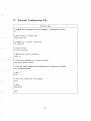
D Example Configuration File
55
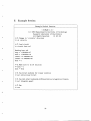
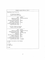
E Example Session
56
F Example Circuit Files
58
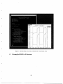
G Example SIMLAB Session
61
iv
A.-
1
Introduction
is a circuit simulation environment consisting of a flexible, user-friendly front-end
operating in conjunction with a sophisticated and versatile simulation engine. The program
SIMLAB
is specifically designed to be used as an educational tool and as a research platform.
SIMLAB
can be operated in either batch or interactive mode.
The user is allowed to separately specify algorithms for the various aspects of the simulation.
These include:
* Simulation environment (e.g. serial or parallel depending on the underlying hardware).
* ODE system solution (e.g. point)
* ODE system time integration (e.g. backward-Euler, trapezoidal, second-order Gear),
* Nonlinear algebraic system solution (e.g. multidimensional Newton's method, nonlinear relaxation),
* Linear system solution (e.g. sparse Gaussian elimination, Gauss-Jacobi relaxation,
conjugate gradient, conjugate gradient squared),
Furthermore,
SIM LAB
has a notion of simulation mode and different methods can be specified
for different modes. At present, supported modes are DC for the calculation of operating
points, and Transient for the calculation of the time response of a circuit. For instance,
assuming that the user has specified the multidimensional Newton's method for solving the
nonlinear system of equations, the linear solver associated could be different depending of
what type of simulation is being performed.
The user can also interactively tune the following simulation parameters:
* stop - final simulation time,
* cmin - minimum capacitance to ground at each node,
* gmin - minimum conductance to ground at each node,
* nrvabs, nrvrel - Newton-Raphson absolute and relative voltage convergence criteria,
* nrcabs, nrcrel- Newton-Raphson absolute and relative current convergence criteria,
* lterel, lteabs - absolute and relative local truncation error,
* nralpha - Newton-Raphson AV step limit,
1
* newj acob - Number of Newton iterations before updating the Jacobian,
* maxtrnr, maxdcnr - Maximum number of transientand dc Newton-Raphson iterations
allowed,
* dodc, dotran - flags indicating dc or transient solution is desired,
* verbose - flag indicating verbose mode,
* simdebug - flag indicating debug mode.
Simulation statistics are also reported for all phases of the simulation process.
In the bibliography, references to standard textbooks and papers on circuit simulation and
related topics are given.
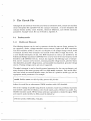
In its basic form, SIMLAB is a powerful circuit simulator, but it is also designed to be easily
customized for research purposes. For example, SIMLAB forms the core of special-purpose
simulation programs, such as a switched capacitor filter simulator and a simulator for vision
circuits. The program code is highly modular, so that researchers can easily construct and
test algorithms by inserting them into the existing SIMLAB framework. For information on
how to add algorithms to SIMLAB see The SIMLAB Programmer's Guide.
The SIMLAB program was developed at MIT under support from Analog Devices, the NSF
PYI program, and DARPA contract N00014-87-K-825. Miguel Silveira was partially supported by the Portuguese INVOTAN committee and Andrew Lumsdaine was also supported
by an AEA/Dynatech faculty development fellowship. Installing SIMLAB in your computer
system is done with the aid of makelinks, a tool for avoiding code duplication developed
at MIT by G. Adams, D. Siegel and S. Narasimhan. The program uses a circuit parser
written by P. Moore and a sparse matrix solver based on work by K. Kundert, both of
whom were students in computer-aided design at U.C. Berkeley. The front-end interpreter
for the program was inspired by the xlisp program written by David Michael Betz and
uses the readline library from the Free Software Foundation's bash program. The plotting
package included with the SIMLAB distribution is xgraph, a two-dimensional plotting package developed by D. Harrison at U.C. Berkeley. Section 3 of this user's manual was derived
in part from R. Saleh's and A.R. Newton's SPLICE User's Manual, available from U.C.
Berkeley.
Question or problems related to the installation or usage of the SIMLAB circuit simulator should be addressed to any one of the authors by U.S. mail, or by electronic mail to
simlab~rle-vsi.mit.edu (18.62.0.214). Any bugs should be reported by electronic mail
to simlab-bugrle-vlsi.mit.edu so that they can be solved for later releases. Furthermore, the authors welcome any comments, suggestions, or enhancements that will come
from other users experience with the program.
2
2
A SIMLAB Primer
SIMLAB is
invoked from the command line as follows:
simlab [-c circuit_file [-r]] [-f diaryfile]
SIMLAB
[-qvV]
configfile]
can be used in interactive mode, in batch mode, or both.
The command line arguments are:
-c circuit specifies a circuit file to be read initially. See the circuit command in Section
A
-f diaryf ile specifies a diary file to be used initially. See the diary command in Section
A
-r specifies that a run is to be executed using the known data. This option requires that
a circuit file be specified and tells simlab to use the default methods to simulate the
given circuit.
-q turns off interactive mode. When this command line argument is given, SIMLAB will
exit after executing the command contained in the specified configuration file. If no
configuration file is given this line argument is ignored.
-v turns on verbose mode, in which case SIMLAB emits certain diagnostic messages. See
the description of the verbose environment variable in Section B.
-V turns on debug mode, in which case SIMLAB emits many diagnostic messages. See the
description of the simdebug environment variable in Section B.
config-file is an initial configuration file read by SIMLAB . If a circuit file is also specified,
the configuration file is read after the circuit file. SIMLAB will read and execute each
line of the configuration file just as if the commands were interactively entered. If
a quit command is not given in the configuration file, SIMLAB will enter interactive
mode after reading it (and executing any commands therein) unless the command
line argument -q is given, in which case SIMLAB exits after executing the command
contained in the configuration file.
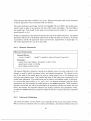
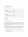
In general, an interactive simulation session will proceed as follows:
1. Start
SIMLAB
(perhaps with a circuit file, configuration file, or both);
2. Configure the simulation environment (interactively, with a configuration file, or
both);
3
3. Run simulation;
4. Plot simulation results;
5. If not done, change circuit parameters and go to 2
When SIMLAB is first started it attempts to read a startup file. SIMLAB first looks for the
file specified by the environment variable SIMLABRC. If this variable is not set, SIMLAB tries
to read, in order, "./.simlabrc" and " /.simlabrc".
2.1
The SIMLAB Front-End
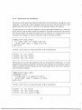
The primary interface to SIMLAB is through an interpretive front-end. The front-end reads
commands and expressions (either interactively or from a configuration file) and evaluates
them. See Appendix A for a description of the available SIMLAB commands.
SIMLAB
will also evaluate expressions. For example, typing in:
=> a = 5 * pi
will produce the result
a = 15.708
Notice that the variable a has been created and now exists in the
you now type
SIMLAB
environment. If
=> a
SIMLAB
will return the value of a:
a = 15.708
has predefined variables (which correspond to certain simulation parameters) that
the user can set via the front-end. These variables include:
SIMLAB
* stop - final simulation time,
* cmin - minimum capacitance to ground at each node,
gin - minimum conductance to ground at each node,
* nrvabs, nrvrel - Newton-Raphson absolute and relative voltage convergence criteria,
* nrcabs, nrcrel - Newton-Raphson absolute and relative current convergence criteria,
4
*
terel, lteabs - absolute and relative local truncation error,
* nralpha - Newton-Raphson AV step limit,
* newj acob - Number of Newton iterations before updating the Jacobian,
* maxtrnr, maxdcnr - Maximum number of transientand dc Newton-Raphson iterations
allowed,
* dodc, dotran - flags indicating dc or transient solution is desired,
* verbose - flag indicating verbose mode,
* simdebug - flag indicating debug mode.
See Appendix B for a complete description of these variables.
The values of these variables can be examined and changed in the obvious way. For instance,
if you type
=> cmin
SIMLAB
will return with the value of cmin, e.g.,
cmin = 1.e-15
To change the value of cmin to 1.0e-12, type in
=> cmin = 1.Oe-12
SIMLAB will
then reply
cmin = 1.e-12
The value of cmin used during simulation will now be 1.0e-12. Note that the predefined
system variables can be used in algebraic expressions. For example, an input line like
=> cmin = stop / 1.Oe-6
is perfectly acceptable. See Appendix B for a complete description of
and the rules that guide their usage and the changes in their values.
2.1.1
SIMLAB
' variables
Command-Line Editing
One handy feature of SIMLAB in interactive mode is its command-line editor, which is
implemented with the readline library of the Free Software Foundation's bash program.
5
The default key-bindings are essentially patterned after gnu-emacs (or tcsh) and allow the
user to recall and edit previous lines.
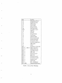
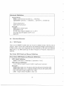
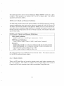
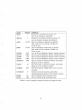
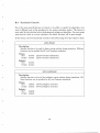
Table 1 shows the most primary key-bindings for the SIMLAB command-line editor. For
more information about readline, refer to the bash documentation from the Free Software
Foundation.
The command-line editor saves each line that is entered into a history list. The history
list can be accessed via the C-n and C-p keys (down and up history, respectively). The
entire history list can be displayed with the history command. The run-time length of the
history list is controlled by the SIMLAB variable histlength. Upon exiting, SIMLAB saves
the history list on a file. The size of the saved history list is controlled by the SIM LAB variable
savehist and cannot exceed the value of histlength. By default upon starting, SIMLAB
looks for the environment variable SIMLABHISTFILE for the location of the history file. If
this variable is not set, SIMLAB will use the default location which is defined at compile time
(normally "./.simlablhist"; see config.h if you desire to change this value).
2.1.2
Plotting
Currently, viewing the results of a simulation run is done using a modified version of xgraph,
a two-dimensional plotting package developed by D. Harrison at U.C. Berkeley. However, if
some local viewing program is available, the user can override the use of xgraph by setting
the environment variable SIMLABPLOTTOOLS to point to the preferred plotting tool. The
environment variable SIMLABPLOTARGS should also be set, possibly with command line
arguments for the plotting tool. If no arguments are necessary, the variable should still be
set (this can be acomplished from inside SIMLAB). Note that the plotting tools must be
able to read the simlab output format which consists of lines of the form:
(nodename) (time) ( voltage)
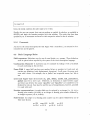
2.2
Specifying algorithms in SIMLAB
One of the most powerful features of SIMLAB (when used for algorithm development)is the
ability to specify which numerical algorithms are used at different stages of the simulation.
For this purpose, there are five basic predefined functional controls:
solvelinear: Specifies function to be used for linear system solution during simulation.
solvenonlinear: Specifies function to be used for nonlinear system solution during simulation.
6
Key
C-a
C-b
C-d
C-e
C-f
C-g
TAB
C-k
C-1
C-n
C-p
C-q
C-r
C-s
C-t
C-u
C-w
C-y
SPC
ESC 0.. ESC 9
ESC b
ESC c
ESC d
ESC f
ESC g
ESC 1
ESC t
ESC u
ESC y
ESC
DEL
ESC DEL
Table 1:
Action
beginning-of-line
backward-char
delete-char
end-of-line
forward-char
keyboard-quit
complete word
kill-line
refresh
down-history
up-history
quoted-insert
isearch-backward
isearch-forward
transpose-chars
universal-argument
kill-region
yank
self-insert-command
digit-argument
backward-word
capitalize-word
kill-word
forward-word
goto-line
downcase-word
transpose-words
upcase-word
yank-pop
list completions
backward-kill-word
SIMLAB
7
Key Bindings.
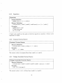
integrate: Specifies which integration method to use.
simulate: Specifies what type of simulation structure to use.
environment: Specifies the environment in which
SIMLAB is being used. This will normally
be serial but functionality to take advantage of parallel computer architectures can
be added.
Furthermore with the notion of simulation mode, some of the above functional controls
can be given different meanings depending on the current mode of simulation. Section B
contains a detailed description of these functional controls. The functional controls are
modified with the set command, and displayed with the show command (see Appendix A).
For example, if you are testing out a new linear system solver called "baz" (and have
properly compiled it into SIMLAB -see
the SIMLAB Programmer's Guide), you would set
the transient linear system solver to baz with
=> set trans solvelinear baz
Or, if baz was a more generic function, you could set it to be the linear solver for all modes
of simulation (namely DC and transient) with
=> set solvelinear baz
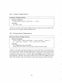
You can examine the settings of the functional controls with show. Typing
=> show solvelinear
will return the current settings for solvelinear for all known modes of simulation. Just
typing
=> show
will return the current settings for all functional controls and simulation modes.
If a functional control is set to a non-existent function, SIMLAB will output a warning and
dismiss the change. However if a change is made to a functional control such that the
new value is incompatible with the current values of other functional controls, SIMLAB will
output an error message at run-time. For instance, suppose that a new simulation method,
called simfoo is compiled into SIMLAB and is such that simfoo uses different data-structures
and therefore requires an integration method called simfooint. If the user merely specifies
=> set simulate simfoo
and then request a run
=> run
8
will try to use the default integration algorithm and will output an error saying
that that algorithm is not a valid setting for the current simulation control.
SIMLAB
2.3
Warnings about the Algorithms used in the SIMLAB Program
One limitation of some popular simulation methods is that they sometimes do not converge
unless there is a capacitor to ground at every node in the circuit. This is a mild assumption
for most realistic circuits, although users of circuit simulators often don't include these
capacitances. Therefore the SIMLAB program will insert a minimum capacitance to ground
at every node in the circuit. This value of the minimum capacitance is set by the parameter
cmin and is a user-alterable, but should not be set to zero.
Finally, the SIMLAB program was developed at MIT as a research project. It is not intended
to be a production system, although serious effort has been made to insure the correctness
of the program (it works for at least one test case). Reporting problems to the authors
about SIMLAB would be appreciated, provided it is done gently.
2.4
Hints on Convergence
Obtaining the DC solution can be a difficult problem, although SIMLAB seems to do a good
job of it. However, there are still examples which will not work. If you have trouble, try
playing with the options gin and nralpha. gin is a conductance placed to ground at
each node, so it should be kept to a reasonable (small) value or your DC solution will not
be accurate. nralpha controls the maximum step a voltage can take in any one iteration of
the DC solution.
does a very good job of converging during the transient solution. In fact, nonconvergence during the transient solution usually means that there is an error in the circuit
or a bug in the program. If you have problems during the transient solution, it may help
to set the option newjacob equal to 1, although this may slow the program down somewhat. Other options include increasing the value of cmin, reducing the absolute and relative
convergence criteria or increasing the maximum number of iterations on iterative solvers.
SIMLAB
9
10
3
The Circuit File
Although the user interacts with SIMLAB in batch or interactive mode, circuits are read from
circuit description files (specified with the circuit command). A circuit description file
contains element models, circuit elements, subcircuit definitions, and selected simulation
parameters. Example circuit files can be found in Appendix F.
3.1
3.1.1
Fundamentals
Models and Elements
The following elements can be used to construct circuits for SIMLAB: linear resistors, linear capacitors, diodes, voltage-controlled current sources, bipolar and MOS transistors.
The BJT transistor model in SIMLAB is an adaption of the integral charge control model
of Gummel and Pool with extensions that include several effects of high bias levels. For
a more detailed description see [8]. The MOS transistors in SIMLAB are modeled by the
Schichmann-Hodges equations [7] (SPICE2 level=1) or by those of the semi-empirical model
described in [8] (SPICE2 level=3). SIMLAB also supports the following types of independent sources: constant current sources, constant grounded voltage sources, piecewise-linear
time-dependent grounded voltage sources, and sinusoidal time-dependent grounded voltage
sources. Floating voltage sources are not yet supported.
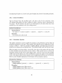
The model statement is used to describe general parameters for the SIMLAB elements, and
many elements of the same type may refer to a single model statement. Each model definition must include an external reference name, the name of a primitive model type, and the
appropriate model parameters. For example:
model BusMos nmos vto=O.8v kp=20u, gamma-0.8 phi=0.6
defines the model for an enhancement NMOS transistor with 0.8V threshold.
The circuit topology is specified using element statements. Each SIMLAB element statement
must include a name for the element, a list of node names, and a reference to a model. So a
BusMos transistor named dWrite2 whose substrate is grounded, is clocked by signal PHI2,
and connects nodes latchOut to DBus would be defined by:
dWrite2 latchOut PHI2 DBus 0 BusMos
11
3.1.2
Subcircuits and Parameters
The SIMLAB circuit parser also supports hierarchical circuit descriptions through the use of
subcircuits. A subcircuit is like a program macro in the sense that the subcircuit is first
defined, and then each time it is referred to, the definition replaces the reference.
The general form for a subcircuit definition is the keyword define followed by a subcircuit
name, and then a list of nodes enclosed in parentheses. The element statements that describe
the subcircuit follow the define statement, and the subcircuit is terminated with an end
statement. For example, an inverter subcircuit could be described as follows:
define inverter (input, output)
ml output input 0 0 pulldn w=10u 1=5u
m2 vdd output output 0 pullup w=5u l=10u
end inverter
and then a circuit that is a string of inverters could be described by
inverter1 inl outi inverter
inverter2 outi out2 inverter
inverter3 out2 out3 inverter
Node names are not the only parameters that can be passed into subcircuits. It is also
possible to pass number parameters to subcircuits. For example, if one wanted to scale the
width of the above inverter, keeping the same width/length ratios, the inverter subcircuit
could be defined as follows:
define inverter (input, output)
parameters w=10u
ml output input 0 0 pulldn w=w 1=0.5* w
m2 vdd output output 0 pullup w=w 1=2.0*w
end inverter
and then a circuit that is a string of inverters could be described by
inverter1 inl outi inverter
inverter2 outi out2 invertsr w=20u
inverter3 out2 out3 inverter w=400u
12
where inverter1 would be assigned the default value of 10 microns for the width.
3.1.3
Locals and Globals
It is possible to have local nodes in a subcircuit. In fact, if any node name that is not
contained in the node list of the define statement for the subcircuit is used in the subcircuit,
it will automatically be local to the subcircuit. This can be overridden by explicitly declaring
certain nodes to be global using the global statement. This is particularly useful for supply
voltage node names. Note, however, that the first node specified on the global list is always
the ground or reference node.
3.1.4
Control Statements
Information such as the simulation period, the simulation accuracy criteria, and analysis
requests, are specified with a single options statement as follows:
simlab options stop=lOOns dodc-1 dotran=l
Default values are used whenever parameter values are not set explicitly by the user. The
value of stop should always be set by the user, as it sets the simulation interval.
In order to request that the output of certain nodes in the circuit are recorded, the plot
statement is used, and its format is just the keyword plot followed by a list of node names.
A warning will be issued if the input file does not specify any nodes for plotting.
3.1.5
Initial Conditions and the DC Solution
The SIMLAB program allows the user two ways of specifying the initial conditions used to
begin a transient analysis. The default is that all the node voltages begin at zero. This
can be thought of as a "power-up" phase. However, the implication of this strategy is that
the circuit should not be clocked until it has settled after powering up. If the circuit is
clocked too early, the simulation will still be performed without error, but the circuit may
not behave as expected.
If desired, it is possible to force a node to be initialized to any voltage by using the ic
statement. Its format is the keyword ic followed by a list of node name, initial value pairs
with the two in each pair connected by an equal sign. For example,
13
ic input=5.O
forces the initial condition for node input to be 5 volts.
Finally, the user can request that
SIMLAB
perform an explicit dc solution, as available in
SPICE2, and begin the transient analysis with that solution. The nodes that have been
specified by an ic statement are forced to their respective values for the dc solution.
3.1.6
Comments
Any line in the circuit description file that begins with a semicolon (;) is assumed to be a
comment line and is ignored.
3.2
Basic Language Rules
Field separators Delimiters may be one of more blanks, or a comma. These delimiters
must be placed where required by the syntax of the circuit description language.
Continuation Character A statement may be continued by ending it with a backslash
(\) and continuing on the next line.
Name Field A name field can have any number letters or numbers in it and must not
contain any delimiters (only alphanumeric characters). In all cases, the name must
start with a letter. For example, alu, or fadder7 are acceptable names, but 7alu is
not.
Lower and Upper Case All keywords (ic, plot, define, model, end, parameters,
global) must be in lower case. Otherwise, no distinction is made between upper
and lower case letters; the names 'signalOne' and 'SignalOne' are considered to be
identical by
SIMLAB.
Case may be used for ease of comprehension, however, provided
it is used with care!
Number representations A number field may be replaced by an integer (i.e. 12, -44), a
floating point number (3.14159), or an integer or floating point number followed by
an integer exponent (1E-14, 2.65e3).
Scale factors An integer or a floating point number can be scaled if followed by one of
these scale factors:
g=lE9
u=lE-6
meg=lE6
n=lE-9
14
k=lE3
p=1E-12
m=lE-3
f=1E-15
Letters immediately following a number that are not scale factors
letters immediately following a scale factor are ignored. Hence, 10,
10Hz all represent the same number, and m, ma, msec, and mmhos
same scale factor. Note that 1000, 1000.0, 1000Hz, 1E3, 1.0E3,
represent the same number.
3.3
are ignored, and
10v, 10volts, and
all represent the
kHz, and k all
Choosing Node Names
Node names A node name can have any number of letters or numbers in it and must not
contain any delimiters (only alphanumeric characters). If the node name is not all
numbers, it must start with a letter. For example, a7, or 17 are acceptable names, but
7a is not.
Ground Node and Global nodes Global names can be used whenever you want to define a node name that is to be used in the main circuit as well as subcircuits. They are
generally used for supply voltage names. Any number of global nodes can be specified
using the global statement. Its format is the keyword global, followed by a list of
node names. The global statement also performs another function, that of indicating
to the SIMLAB program which node to use as ground. The first node in the global
node list is assumed by SIMLAB to be the ground node, and should be so specified.
There is no other constraint on the order of the nodes in the list.
3.4
General Form for Model and Element Statements
Notation In the following description, data fields that are enclosed in brackets, '[' and
']' are optional. Names enclosed in '(' and ')' should be replaced by alphanumeric
strings and value fields should be replaced with numbers. All indicated punctuation
is required. Associated reference directions are used (positive current flows in the
direction of most positive to most negative).
3.4.1
Model Statements
Model Statement
General Form:
model (name) (type) [[ (namel) = (value) ] [(name2) = (value) ]...]
Examples:
model nmosl nmos vto-=2v kp=15u gamma=0
model cstray c c=0.025pf
15
This statement describes a model in the circuit. Element statements refer to this statement
to obtain parameter values associated with the element.
The model statement must begin with the word model. The next field is the model name,
which is used to refer to the model in the rest of the circuit description. The third field is
the model type. This should be the name of an internal SIMLAB model (r, c, nmos, pmos,
nmos3, pmos3, d, etc).
If there are parameters, they should be listed at the end of the model statement. All unlisted
parameters will be set to the default value for the model type (See next section). To specify
a parameter, include the parameter name and the value, separated by an equal sign (=).
The model parameters list can be in any order.
3.4.2
Element Statements
Element Statements
General Form:
( name ) (nodel )
...
(nodeN) ( model or subcircuit name) (params)
Examples:
nmosl store input phase 0 mostran w=25u 1=1.5u
gcapl input output c c=0.07p
gate7 output outbar inverter
The element definition statement consists of an element name, the nodes connected to the
element, a model to which the element refers, and optional parameters. The element names
can be the same as the model name (or even as a node name), but no two elements may
have the same element name. The number and order of the nodes must correspond to the
model being referenced. The model name can be either a user defined model, a subcircuit,
or a SIMLAB low-level model (c, r, dc, pwl, i, etc.). An element statement can also include
parameters, and will override the values given in the model statement. MOS transistor
elements can include the width (w) and length (1) parameters, diodes can include the area
factor, and resistor and capacitor elements can include resistance and capacitance values.
As with the model statement, parameters should be listed as a name/value pair, separated
by "=".
3.4.3
Subcircuit Definitions
The subcircuit defines a macro which can be expanded in the circuit any number of times.
When an element statement refers to a subcircuit definition, the elements defined within the
16
subcircuit are inserted into the circuit. The node names specified in the element statement
are substituted for the node names in the subcircuit definition statement. This substitution
is by order, the first node in the element statement is substituted for the first node in the
subcircuit definition, and so on. Note that the node names in the subcircuit definition must
be enclosed in parentheses, and that it is an error for the element statement to have a
different number of nodes than the subcircuit definition it refers to.
Any nodes used within the subcircuit which are not global (contained on the global node
list), and are not listed in the subcircuit definition statement, are local to that subcircuit
(i.e. these names are not known outside the subcircuit definition). Since a global node
cannot be replaced during a subcircuit expansion, it is an error for a global name to appear
as a node on a subcircuit definition statement.
The subcircuit can optionally include a parameters statement. To specify subcircuit parameters, the keyword parameters is followed by a list of parameter names and default
values, separated by equals (=). A named parameter can be used as if it were a number
in the subcircuit description, and in addition, can be multiplied by a floating point number
scale factor. An element statement which refers to the subcircuit can set the values of any
or all of the names parameters. Any parameters that are not set on the element statement
will be given its default value.
The most recently begun subcircuit is terminated by the end statement. An optional name
may be specified after the end statement to indicate which subcircuit definition is being
completed. This name is not used by the program but is useful to include for readability.
Internal subcircuit nodes may be referenced for plotting or for assigning initial conditions,
by using a name derived from its subcircuit node name and the subcircuit instance name
separated by a dot ".". For example, "adderl.il" refers to internal node "i1" in a subcircuit
instance called "adderi".
17
Subcircuit Definitions
General Form:
define ( subcircuitname) (( node 1 ) [... (node N )])
[parameters (paraml) = (default) [... (paramN) = (default)]]
(element statements)
end [(subcircuitname)]
Example:
define invert (output input)
parameters w=5u
ml vdd output output 0 depload w=w 1=1.0* w
m2 output input 0 0 pulldn w=5.0* w l=w
end invert
3.5
Electrical Elements
3.5.1
MOS Models
There are two MOSFET models that can be used to simulate circuits with the SIMLAB
program. There is a first order model based on the Schichmann-Hodges equations[4] for the
dc drain current, and a more complicated one whose equations are the same as for SPICE2
MOS Level 3. An MOS model may be either N-channel or P-channel, enhancement or
depletion.
First Order MOS Model and Element Definitions
First Order MOS Model and Element Definitions
MOS Model Definition:
model ( model name ) ( model type) [(parameter- list)]
MOS Element Definitions:
(name) (drain) (gate) (source) (bulk) (model name) (params)
Examples:
model pullup nmos vto=-5.2 gamma=0.914 kp=69u phi=0.6 lambda=0.02
model pulldn pmos vto=1.12 gamma=0.266 kp=79u phi=0.6 lambda=0.02
loadl vdd output output 0 pullup w=5u 1=20u
pulldn output outbar 0 0 pulldn w=-10u 1=5u
18
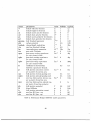
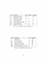
The model parameters used in SIMLAB Schichmann-Hodges MOSFET model are as given
in Table 2. Any parameter not specified will be set to its default value. The element
parameters are listed in Table 3.
MOS Level 3 Model and Element Definitions
The MOS level 3 model is based on the model available in the SPICE2 program [6], although
numerous modifications have been made to enhance the speed and insure the accuracy of
the model. This model is suitable for small geometry MOSFETs and it accounts for secondorder effects such as threshold voltage sensitivity to the length and width of the device and
lowered saturation voltage and current due to velocity saturation. The details of this model
may be found in [8]
MOS Level 3 Model and Element Definitions
MOS Model Definition:
model (model name) (model type) [( parameter- list)]
MOS Element Definitions:
(name) (drain) (gate) (source) (bulk) (model name) (params)
Examples:
model pullup nmos3 vto=-5.2 gamma=0.914 kp=69u phi-0.6 lambda=0.02
model pulldn pmos3 vto=1.12 gamma=0.266 kp=79u phi=0.6 lambda=0.02
loadl vdd output output 0 pullup w=5u 1=20u
pulldn output outbar 0 0 pulldn w=10u 1=5u
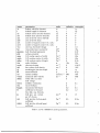
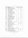
The model parameters used in MOS Level 3 are listed in table 4. The element parmeters
for the MOS 3 model are listed in table 6.
3.5.2
Bipolar Models
There is a BJT model that can be used to simulate circuits with bipolar transistors with
the SIMLAB program. This model is an adaption of the integral charge control model of
Gummel and Pool with extensions that include several effects of high bias levels.
19
name
w
1
as
ad
ps
pd
gamma
phi
lambda
vto
kp
tox
cgso
cgdo
cgbo
fc
js
mj
mjsw
Ci
CjSW
cjsw
pb
ld
is
cbd
cbs
parameter
default width for elements
default length for elements
default source area for elements
default drain area for elements
default source perimeter for elements
default drain perimeter for elements
bulk threshold parameter
surface potential
channel-length modulation
zero-bias threshold voltage
transconductance parameter
gate oxide Thickness
gate-source overlap capacitance
per unit channel width
gate-drain overlap capacitance
per unit channel width
gate-bulk overlap capacitance
per unit channel width
coefficient for forward-bias
depletion capacitance formula
bulk junction saturation current
per sq-meter of junction area
bulk junction bottom grading coef.
bulk junction sidewall grading coef.
zero bias bulk junction bottom cap.
per sq-meter of junction area
zero bias bulk junction sidewall cap.
per meter of junction perimeter
bulk junction potential
lateral diffusion
bulk junction saturation current
zero-bias B-D junc. cap
zero-bias B-S junc. cap
units
m
m
m
Fm-'
default
1
1
0
0
0
0
0
0.6
0
0.0
20t
0
0
40p
Fm - 1
0
40p
Fm - 1
0
200p
0.5
0.5
Am-2
0
lOn
Fm- 2
0.5
0.5
0
0.5
0.33
0.2m
0
in
0.8
0
0
0
0
0.87
0.8yu
if
20f
20f
m2
m
2
m
m
vl/2
V
V-1
V
AV-2
V
m
A
F
F
Table 2: Schichmann-Hodges MOSFET model parameters.
20
typical
1l t
2p
0
0
0
0
0.37
0.65
20m
1
lo0
My
0.17
name
w
1
parameter
channel width
channel length
as
area of source region
ad
ps
pd
area of drain region
perimeter of source region
perimeter of drain region
units
m
m
m2
m2
m
m
examples
lO
1.5p
loop
loo00p
40y
40/
Table 3: Schichmann-Hodges MOSFET element parameters.
Bipolar Transistor Models
BJT Model Definition:
model (model name) (model type) [(parameter - list ) ]
BJT Element Definitions:
( name) (collector) (base) emitter) (substrate) model name ) (params)
Examples:
model nbjt npn bf=200 vaf=250 tr=10n
model pbjt pnp
loadl vdd 3 5 0 nbjt
pulldn 1 output outbar 0 0 pbjt bf=100
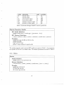
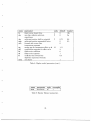
The model parameters used in SIMLAB BJT model are as given in Table 7. Any parameter
not specified will be set to its default value. The element parameters are listed in Table 9.
3.5.3
Diodes
Diodes
Model Definition:
model (name) d [(parameters)]
Element Definition:
( element name) ( anode) ( cathode) ( model name) [area = (value ) ]
Example:
model pnj d cjO=Se-12
dl drain pnj area=2p
d2 0 source pnj area=2p
21
name
w
1
as
ad
ass
asd
nrs
nrd
vto
kp
gamma
phi
cgso
cgdo
cgbo
tox
nsub
nfs
xj
ld
uo
vmax
delta
theta
eta
kappa
fc
js
mj
mjsw
parameter
default width for elements
default length for elements
default source area for elements
default drain area for elements
area of the fet source sidewall
area of the fet drain
number of squares (source res. calc.)
number of squares (source res. calc.)
zero-bias threshold voltage
transconductance parameter
bulk threshold parameter
surface potential
G-S overlap cap/m of width
G-D overlap cap/m of width
G-B overlap cap/m of length
oxide thickness
substrate doping
fast surface state density
metallurgical junction depth
lateral diffusion
surface mobility
maximum drift velocity
width effect on threshold voltage
mobility modulation
static feedback
staturation field factor
coefficient for forward
bias delp. cap. formula
bulk junc. sat. current
per m 2 of area
bulk junction bottom grad.
coefficient
bulk junction sidewall grad.
coefficient
units
m
m
m2
m2
m2
m2
defaults
1
1
0
0
0
0
0
0
0
0
0
0
0
0
0
10o
0
0
0
0
600
0
0
examples
ly
2/
0
0
0
0
0
0
1.0
10/
0.37
0.65
40p
40p
0.2n
10p
4.0e15
10G
1l/
0.81
700
50K
1
0
0
0.2
0.2
0.1
1
0.5
1.2
Am- 2
0
if
Fm- 2
0.5
0.2m
Fm- 2
0.5
0.2m
V
AV 2
V1 / 2
V
Fm -1
Fm -1
Fm - 1
m
cm - 3
cm - 2
m
m
cm 2 (Vs) ms- 1
Table 4: Level 3 MOSFET model parameters.
22
name
cj
cjsw
pb
rs
rd
nss
is
parameter
zero-bias junc. bottom
capacitance/m 2 of area
zero-bias junc. sidewall
capacitance/m 2 of area
bulk junc. potential
source resistance (per square)
drain resistance (per square)
surface state density
bulk junc. sat. current
units
Fm- 2
defaults
0
examples
0.2m
Fm - 2
0
0.2m
V
Q
Q
cm - 2
A
0.8
0
0
0.lm
l10f
0.87
0
0
10G
If
Table 5: Level 3 MOSFET model parameters (cont.).
name
w
1
parameter
channel width
channel length
units
m
m
examples
10,
1.5y
as
area of source region
m2
loo100p
ad
ps
pd
nrs
nrd
area of drain region
perimeter of source region
perimeter of drain region
number of squares (source res. calc.)
number of squares (source res. calc.)
m2
m
m
0
0
loo100p
40y
40p
10
10
Table 6: Level 3 MOSFET element parameters.
23
name
is
bf
nf
vaf
ikf
ise
ne
br
nr
var
ikr
isc
nc
rb
irb
rbm
re
rc
cje
vje
mje
tf
xtf
vtf
itf
ptf
cjc
vjc
mjc
xcjc
parameter
transport saturation current
ideal maximum forward beta
forward current emission coefficient
forward Early voltage
corner for forward beta
high current roll-off
B-E leakage saturation current
B-E leakage emission coefficient
ideal maximum reverse beta
reverse current emission coefficient
reverse Early voltage
corner for reverse beta
high current roll-off
B-C leakage saturation current
B-C leakage emission coefficient
zero bias base resistance
current where base resistance
falls halfway to its min value
minimum base resistance
at high currents
emitter resistance
collector resistance
B-E zero-bias depletion capacitance
B-E built-in potential
B-E junction exponential factor
ideal forward transit time
coefficient for bias dependence of tf
voltage describing vbc
dependence on tf
high-current parameter
for effect on tf
excess phase at f =
Hz
B-C zero-bias depletion capacitance
B-C built-in potential
B-C junction exponential factor
fraction of B-C depletion capacitance
connected to internal base node
units
A
default
10f
100
1
oo
c
typical
if
200
1
200
0.01
0
1.5
1
1
c
oo
0.ln
2
0.1
1
200
0.01
Q
A
0
2
0
c
0.ln
1.5
100
0.1
Q
rb
10
F
V
s
0
0
0
0.75
0.33
0
1
10
2p
0.6
0.33
0.ln
s
0
0
V
cc
A
0
deg
F
V
0
0
0.75
0.33
1
V
A
A
V
A
A
Table 7: Bipolar model parameters.
24
2p
0.6
0.5
name
tr
cjs
vjs
mjs
xtb
eg
xti
kf
af
fc
area
parameter
ideal reverse transit time
zero-bias collector-substrate
capacitance
substrate junction built-in potential
substrate junction exponential factor
forward and reverse beta
temperature exponent
energy gap for temperature effect on is
temperature exponent for effect on is
flicker-noise coefficient
flicker-noise exponent
coefficient for forward-bias
depletion capacitance formula
area factor
units
s
F
default
0
1
0
typical
on
2p
V
0.75
0
0
0.6
0.5
eV
1.11
3
0
1
0.5
1
Table 8: Bipolar model parameters (cont.).
name
area
parameter
area factor
units
m2
examples
1
Table 9: Bipolar Element parameters.
25
name
area
is
imax
n
tt
vt
cjo
phi
m
fc
bv
parameters
diode area
saturation current
Forward explotion
current
emission coefficient
transit-time
thermal voltage
zero-bias junc. cap.
junction potential
grading coeff.
coeff. of depletion
cap. in forward bias
rev. breakdown
units
m2
A
A
s
V
F
V
V
default
1
lOf
10
typical
l
1.5p
10
1
0
2.58n
0
0.6
0.5
0.5
1
0.In
2.58n
2p
0.6
0.5
0.5
00
40
Table 10: Diode model parameters.
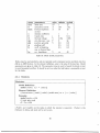
Diodes may be used anywhere, and are typically used to represent source and drain junction
effects on MOS devices. In the element definition, area is the area of the junction. Model
parameters are given in table 10. The parameter imax is used to bound the diode current
to avoid numerical overflow. It should be set to a value that well above a reasonable current
for the diode.
3.5.4
Resistors
Resistors
Model Definition:
model (name) r [r = (value)]
Element Definition:
( element name ) ( nodel ) ( node2) ( model name ) or r [r = ( value ) ]
Example:
model rmod r r=15k
rl input gate rmod
r2 1 2 r r=lOk
( Nodel ) and ( node2 ) are the nodes to which the resistor is connected. (Value) is the
resistance in ohms, and must not be set to zero.
26
Capacitors
3.5.5
Capacitors
Model Definition:
model (name) c [c = (value)]
Element Definition:
(element name) (nodel ) ( node2) ( model name) or c [c = (value ) ]
Examples:
model cmod c c=5uf
cl input gate cmod
c2 1 2 c c=15P
( Nodel ) and ( node2 ) are the nodes to which the capacitor is connected. (Value) is the
capacitance in farads.
3.5.6
Constant Current Source
Constant Current Source
Element Definition:
( element name) (nodel ) ( node2 ) i i = (value)
Example:
biasl 1 2
i i=20ua
The current ( value ) (in amperes) flows from ( nodel ) to (node2).
3.5.7
Voltage Controlled Current Source
Voltage Controlled Current Source
Element Definition:
( element name) (nodel ) (node2 ) (node3) (node4 ) vccs gm= (value)
Example:
vccsl 1 2 3 4 vccs gm=3
The current (value) x (v3 - v4) flows from (node1 ) to ( node2 ).
27
3.5.8
Constant Voltage Sources
Constant Voltage Sources
Element Definition:
(element name) (node 1) (node2) dc v = (value)
Example:
vcc 1 0 dc v=5.0v
( Nodel ) is the positive node of the voltage source, and ( node2) must be the ground node.
SIMLAB does not yet support floating voltage sources.
3.5.9
Piecewise-linear Voltage Sources
Piecewise-linear Voltage Sources
Element Definition:
(name) (nodel ) (node2) pwl [delay = (value) (period) = (value ) ]\
tO = (value) vO = (value) [... t24 = (value) v24 = (value)]
Example:
vin 1 0 pwl delay=Ons period=0lns \
tO-=Ons vO=-5.0v tl=lOns vl=5.0v t2=15ns v2=0.Ov t3=95ns v3=Ons
( Nodel ) is the positive node of the voltage source, and ( node2 ) must be the ground node.
does not yet support floating voltage sources. There are three types of parameters
for the pwl. There can be up to 20 ( through 19) breakpoints in the piecewise linear
waveform, which are pairs (ti=sec vi=volts). There is also a delay parameter, which causes
each breakpoint is delayed by the amount specified. Finally, there is the period parameter,
which, when specified, causes the waveform to repeat after the given number of seconds.
SIMLAB
28
3.5.10
Sinusoidal Voltage Sources
Sinusoidal Voltage Sources
Element Definition:
( element name) (nodel ) ( node2 ) sine \
[phase = (value) freq = (value) ampl = (value) offset = (value)]
Example:
vin 0 sin ampl=lv freq=lk
( Nodel ) is the positive node of the voltage source, and ( node2 ) must be the ground node.
SIMLAB does not yet support floating voltage sources.
3.6
Analysis and Control Statements
3.6.1
Plot Statement
The only way to specify desired output from a SIMLAB simulation is with the plot statement,
and therefore every circuit description file should have this statement. All the nodes to be
plotted must be listed after the plot keyword, and this keyword should appear only once
in a circuit description file. There is no limit to the number of plotted nodes, but it is an
error to try to plot an unused node. In the third example above, latchl1 and latch2 are two
subcircuit instances with the internal node store.
Plot Statement
General Form:
plot (nodel ) [(node2) [... ( node N )]]
Examples:
plot clock j k q qbar
plot phasel phase2 latchl.store latch2.store
For each node name following the plot keyword SIMLAB will produce an entry in the output
file with the node name, time, and voltage. The file will have the same name as the circuit
file, except with a ".trans" extension. The plot file contains a collection of time-voltage
pairs. This format was chosen because it allows the end-user to write a post-processor to fit
a given terminal with the minimum of effort (in fact, the plot command available from the
front-end spawns a post-processor to read the plot file). Note that if accuracy is critical,
the points should be interpolated with a 2-order Lagrange polynomial. However, linearly
29
interpolating the points is, in most cases, good enough and produces reasonably good plots.
3.6.2
Initial Conditions
The ic statement forces the specified node to the given value for the calculation of the
DC solution, after which, the node is allowed to take on whatever value is determined by
the circuit. The DC solution uses zero for an initial guess for all nodes other than those
specified by an ic statement or set by a voltage source.
Initial Conditions
General Form:
ic (nodel) = (value ) (node2) = (value2) ... (node N) = (value N)
Example:
ic a=5.0 b=0.2 c=0.3 d=5.0
3.6.3
Simulation Options
The options statement is used to specify the analyses to be performed, and the balues of
simulation parameters to be used. These options, their defaults and an explanation of each
is given in Table 11. With the exception of dodc, dotran, and stop, these parameters
should only be adjusted by an informed user. The defaults should work well for most cases.
When an option is set from within a circuit file, that value of the option will only apply
for that simulation and until another circuit is read in. When another circuit is read in, all
simulation options are first reset to their default values. The new circuit may then possibly
modify some of the options, but those modifications would only apply to that particular
circuit. The default values of these options can be modified from the front-end. See Section
B.2 for a more detailed explanation of the behavior of the simulation options.
Simulation Options
General Form:
simlab options [(paraml) = (valuel) ... (paramN) = (value N ) ]
Examples:
simlab options stop=lOOns dodc=O
simlab options stop=lOOns cmin=le-16
30
name
dodc
default
1
dotran
5m
10m
definition
If equal to 1, performs dc solution. If
zero, no dc solution is performed.
If equal to 1, performs transient analysis. If
zero, no transient analysis is performed.
Sets the minimum capacitance to ground.
Only used in the dc solution. Should not
be set to zero.
Sets the minimum conductance to ground.
Only used in the dc solution. Should not
be set to zero.
sets the Newton-Raphson absolute voltage tolerance.
Sets the Newton-Raphson relative voltage tolerance.
Sets the Newton-Raphson absolute current tolerance.
Sets the Newton-Raphson relative current tolerance.
Sets the number of newton iterations used before
giving up in the dc solution.
Sets the number of newton iterations used before
giving up in the transient solution.
Sets the maximum voltage step to use in newton
iteration.
Number of newton iterations used before
reevaluating the jacobian in the transient analysis.
Sets the absolute local truncation error.
Sets the relative local truncation error.
SIMLAB
program simulation options and default values.
1
cmin
le-18F
gmin
lnmho
nrvabs
nrvrel
nrcabs
nrcrel
maxdcnr
maxnr
lmV
0.001
le-9
0.001
200
10
nralpha
0.3V
newjacob
3
lteabs
lterel
Table 11:
31
32
A
SIMLAB Commands
cd
cd
Purpose:
Change current working directory
Synopsis:
cd [ pathname ]
Description:
cd changes the current working directory, i.e., the starting point for pathnames not
beginning with '/'. Without an argument, cd changes to the user's home directory.
The cd command understands the csh style of - shorthand for pathnames.
circuit
circuit
Purpose:
Load a circuit file for simulation
Synopsis:
circuit filename
Description:
circuit loads a circuit into SIMLAB for simulation. "filename" must be a valid file
name. Some application variables will be affected by the circuit file.
Diagnostics:
The input circuit file must be specified in
information.
33
SIMLAB
format. See Section 3 for more
continue
continue
Purpose:
Continue simulation run.
Synopsis:
continue
Description:
continue allows the user to continue a simulation run from the present time until
stop. This is useful when a run is made and the stop time increased, or when a
run is interrupted. Transient simulations started with continue begin at time t =
PresentTime and end at time t = stop.
Diagnostics:
If the present time equals the stop time, continue does nothing. If continue isissued
without a previous run, a run is executed.
34
diary
diary
Purpose:
Record the session in a file.
Synopsis:
diary [on / off
[filename ]
Description:
The diary command saves the entire SIMLAB session (in ascii format) in file filename.
If no "filename" argument is specified, the session is saved (in ascii format) in the file
"diary.doc." The argument off will temporarily suspend diary operation until diary
on is issued.
The diary command will also save output generated by programs run with escapes
to the shell.
Diagnostics:
Diary uses tee to capture output produced by programs run in an inferior shell. Some
programs (in particular, s) have a different format when directing output to a pipe
instead of to the standard output.
35
help
help
Purpose:
Provide help.
Synopsis:
help [item ]
Description:
help provides help. When invoked without an argument, help provides a list of
possible help topics. When invoked with an argument, help provides information on
that specific topic.
Diagnostics:
At present, help can only list possible help topics. On-line help will be enhanced in
future releases.
history
history
Purpose:
List previous command lines.
Synopsis:
history
Description:
history lists the lines entered into SIMLAB for review by the user. Previous lines can
be accessed with successive applications of the C-p key (see Section 2.1.1).
36
plot
plot
Purpose:
Plot the circuit output.
Synopsis:
plot
Description:
plot causes all the nodes specified in the circuit input file (using the circuit description
file plot directive, which is distinct from the SIMLAB plot command) to be plotted.
See Sections 2.1.2 and 3.6.1.
Diagnostics:
SIMLAB effects this command by forking and calling an appropriate plot program
for its host environment. Presently, only the X-windows version 11 environment is
supported. At this time, all the nodes specified by the plot line in the circuit file will
be plotted - individual nodes cannot be selected from that list. This should change
in a future release.
printenv
printenv
Purpose:
Print the value of an environment variable.
Synopsis:
printenv [ env-var]
Description:
printenv prints out the values of the variables in the UNIX environment of the
process. If a variable is specified, only its value is printed.
37
SIMLAB
quit
quit
quit~~~~~~~~~~~~~~~~~~~~~
quit
Purpose:
Leave SIMLAB
Synopsis:
quit
Description:
The quit command terminates the current
closed.
SIMLAB
session. Any open diary file is
run
run
Purpose:
Perform a simulation.
Synopsis:
run
Description:
The run command begins a simulation run. If the dodc variable is set TRUE, a DC
solution is initially attempted. If the dotran variable is set, a transient simulation is
attempted. Transient simulations started with run begin at time t = 0 and end at
time t = stop. The user can stop a simulation in progress by typing ctrl-c.
38
set
set
Purpose:
Set simulation parameter.
Synopsis:
set [ mode ] param val
Description:
The set command assigns value "val" to parameter "param" in mode "mode". If no
mode is specified the parameter is assigned value "val" irrespective of the simulation
mode. "val" must be a valid value for "param". See Section B for a description of
available parameters and values.
setenv
setenv
Purpose:
Set environment variable.
Synopsis:
setenv[ env var [ val ]
Description:
With no arguments, the setenv command displays all UNIX environment variables.
With the envval argument it sets the environment variable envvar to have an empty
(null) value. (By convention, environment variables are normally given upper-case
names.) With both envvar and val arguments setenv sets the environment variable
envvar to the value val, which must be either a single word or a quoted string.
When SIMLAB is started all the environment variables currently set are automatically
imported to the SIMLAB UNIX environment. Setting a new variable or reseting the
value of an existing variable affectes the UNIX environment of SIMLAB but not that
of its father process.
39
sh
sh
sh
sh
Purpose:
Execute shell command
Synopsis:
sh [command]
Description:
sh executes its arguments using an inferior shell. If nor arguments are given, sh will
start up the shell specified by the SHELL environment variable, or /bin/sh if the SHELL
environment variable is not set.
For example:
=> sh ls
will execute the ls command in the current working directory.
Diagnostics:
The inferior shell when sh isinvoked with arguments is sh not csh, so certain csh
features will not work (in particular the for pathnames).
40
show
show
Purpose:
Show
SIMLAB
parameters and values.
Synopsis:
show [[ mode ]] param]
Description:
The show command displays SIMLAB parameters and values. With an argument, show
displays the specified parameter and values for the various modes. If a mode is also
specified along with a parameter then only the value of that parameter for the mode in
question is shown. Without an argument, show displays all the parameters and their
values for the various modes. See Section B for a description of available parameters
and values.
source
source
Purpose:
Load and execute a
SIMLAB
configuration file.
Synopsis:
source filename
Description:
The source command causes
SIMLAB
to read and execute a
SIMLAB
configuration file.
Diagnostics:
attempts to interpret everything in the specified file. Funny things can happen
if it is given a file which is not a SIMLAB script.
SIMLAB
41
unsetenv
unsetenv
Purpose:
Unset environment variable.
Synopsis:
unsetenv env var
Description:
unsetenv removes the variable "env var" from the UNIX environment.
who
Purpose:
Display variables existing in the
who
SIMLAB
environment.
Synopsis:
who
Description:
The who command displays the variables existing in the SIMLAB environment. The
variables are grouped into three categories, system constants, application variables,
and user-defined variables. See Section B for a description of SIMLAB environment
variables.
42
B
SIMLAB Variables
B.1
System Constants
True
Description:
Boolean value True. Can be used with boolean simulation variables, e.g., dodc =
True. True is equivalent to integer value one.
False
Description:
Boolean value False. Can be used with boolean simulation variables, e.g., dodc =
False. False is equivalent to integer value zero.
pi
Description:
3.14159 ....
B.2
Simulation Variables
These variables are used for controlling various aspects of the simulation. You will most
likely only need to change those variables which are necessary to specify the type of simulation desired, e.g., stop, dodc, or dotrans. In general, the default values of the other
variables will work well. If convergence problems are encountered, you may wish to adjust
some (see Sections 2.3 and 2.4).
In the current release of SIMLAB all variables can be changed by the user when interacting
with the front-end. Some of them, however, can also be set from the circuit file. SIMLAB
has the notion of default value of a variable and current value of a variable. Changes in the
default or current values of SIMLAB's variables adhere to the following conventions:
1. all changes to values of SIMLAB'S variables, affecting either their default or current
values, are shown to the user;
2. before any circuit is read into SIMLAB, the current values of all SIMLAB variables are
reset to their default values;
43
3. if the value of a SIMLAB variable is set at the command line that change affects both
the default and current values of that variable; furthermore the new value becomes
the new default value for the entire session;
4. if the value of a SIMLAB variable is set from the circuit file, that change affects only the
current value, although it remains in effect until a new value is given at the command
line or a new circuit is read.
This means that reading in circuits that explicitely contain commands to change the value
of some of SIMLAB'S variables will not affect subsequent runs of other circuit, since the
variables are reset to their default values before a new circuit is read into SIMLAB. However
setting the value of a variable at the command line changes the actual default value of the
variable for the entire SIMLAB session.
time
Description:
The current value of time in the simulation run. time is set to zero when run is
issued, and should be set to stop when a simulation run is completed normally.
cmin
Description:
Minimum value of capacitance to ground at each node. Should not be set to zero.
Default:
1.Oe-18 F
dodc
Description:
Boolean variable specifying whether or not to conduct a dc simulation. If dodc and
dotran are both set to True, the dc simulation is conducted first and the solution
is used as the initial condition for the transient simulation.
Default:
True
44
dotran
Description:
Boolean variable specifying whether or not to conduct a transient simulation. If
dodc and dotran are both set to True, the dc simulation is conducted first and the
solution is used as the initial condition for the transient simulation.
Default:
True
gmin
Description:
Minimum condutance to ground at each node. Should not be set to zero.
Default:
lp mhos
histlength
Description:
Size of the history list to be kept by
SIMLAB
Default:
100
lteabs
Description:
Absolute local truncation error tolerance.
Default:
5m
lterel
Description:
Relative local truncation error tolerance.
Default:
lom
45
at run-time.
maxdcnr
Description:
Maximum number of newton iterations in the dc simulation to be attempted before
indicating failure.
Default:
200
maxnr
Description:
Maximum number of newton iterations in the transient simulation to be attempted
before indicating failure.
Default:
10
maxsteps
Description:
The simulation interval divided by maxsteps yields the smallest allowable timestep.
Default:
1.0e8
minsteps
Description:
Minimum allowable number of steps in simulation interval.
Default:
50
newjacob
Description:
Number of newton iterations used before re-evaluating Jacobian.
Default:
3
46
nralpha
Description:
Maximum allowable voltage step in Newton iteration update.
Default:
0.3
nrcabs
Description:
Absolute Newton current error tolerance.
Default:
in
nrcrel
Description:
Relative Newton current error tolerance.
Default:
im
nrvabs
Description:
Absolute Newton voltage error tolerance.
Default:
im
nrvrel
Description:
Relative Newton voltage error tolerance.
Default:
Im
47
savehist
Description:
Size of the history list to be saved upon exiting
SIMLAB.
Default:
100
simdebug
Description:
Flag indicating simdebug mode. This is a debugging mode and a large amount of
diagnostic messages are printed. There should never be any reason to set simdebug
to True.
Default:
False
stop
Description:
stop specifies the length of the transient simulation interval. Transient simulations
started with run begin at time t = 0 and end at time t = stop. Transient simulations started with continue begin at time t = PresentTime and end at time
t = stop.
Default:
s
verbose
Description:
Flag indicating verbose mode. This is a debugging mode and a large amount of
diagnostic messages are printed. There should never be any reason to set verbose
to True.
Default:
False
48
1.
B.3
Functional Controls
One of the most powerful features of SIMLAB is the ability to specify the algorithms to be
used at different levels of the simulation for the various simulation modes. This feature is
most useful for the individual who is developing and testing new algorithms. For most people
using SIMLAB strictly as a circuit simulator, the default functions will be good enough.
In this section, the seven functional controls are described, along with valid values for them.
solvelinear
Description:
Specifies function to be used for linear system solution during simulation. Different
functions can be specified for DC and Transient simulation.
Values:
(dc)
(tran)
direct
direct
Default:
(dc)
(tran)
direct
direct
(sparse Gaussian elimination)
(sparse Gaussian elimination)
solvenonlinear
Description:
Specifies function to be used for nonlinear system solution during simulation. Different functions can be specified for DC and Transient simulation.
Values:
(dc)
(tran)
newton
newton
Default:
(dc)
(tran)
newton
newton
(Newton-Raphson iteration)
(Newton-Raphson iteration)
49
integrate
Description:
Specifies which integration method to use. Has no meaning except in transient
mode.
Values:
(tran)
(tran)
(tran)
(tran)
trap
gear2
beuler
feuler
(trapezoidal integration)
(second-order backward-difference integration)
(backward-Euler integration)
(forward-Euler integration)
Default:
(tran)
trap
simulate
Description:
Specifies what type of simulation structure to use. Different functions can be specified for DC and Transient simulation.
Values:
(dc)
(tran)
pt
pt
(pointwise solution in time)
(pointwise solution in time)
Default:
(dc)
(tran)
pt
pt
50
environment
Description:
Specifies what type of environment SIMLAB was built for. Different environments
cannot be specified for DC and Transient simulation. The value reflects the nature
of the underlying hardware and is therefore likely to suffer little if any changes.
The notion of environment is included to allow expandability to different computer
architectures such as was done with CMVSIM[5, 4], the vision circuit simulator
developed on the Connection Machine[3].
B.4
Values:
(dc)
(tran)
serial
serial
Default:
(dc)
(tran)
serial
serial
(sequential computer environment)
(sequential computer environment)
Environment Variables
SIMLABPLOTTOOL
Description:
Specifies which program to use for plotting node waveforms when the plot command is used. This program must be in the user's PATH. By default SIMLAB uses
SIMGRAPH, a modified version of the XGRAPH program.
SIMLABPLOTARGS
Description:
Contains command line arguments to be used when invoking SIMLABPLOTTOOL for
plotting node waveforms. It is disregarded if the default tool, SIMGRAPH is used.
SIMLABHISTFILE
Description:
Specifies the location and name of the file to use as history file. If not set,
SIMLAB will use the default naming specified at compilation time (normally
"./. simlablhist").
51
SIMLABRC
Description:
Specifies the location and name of the default SIMLAB configuration file. This file
is read by SIMLAB at startup time. If this variable is not set, SIMLAB tries to read,
in order, "./. simlabrc" and " /. simlabrc".
52
C
Non-Standard Supported Packages
Currently
SIMLAB
supports two packages not included under what is called the standard
functionality. These are the Iterative Linear System Solution package and the Wave-
form Newton Circuit Simulation package. These packages are examples of the powerfulness of SIMLAB as a tool for research in circuit simulation algorithms and are provided
together with the standard distribution. However to be able to use the functionality they
provide, SIMLAB must be told to incorporate these packages when building an executable.
This is accomplished by proper setup of the options provided in the config.h configuration
file.
The mentioned packages were built on top of SIMLAB and have been tested perhaps less
frequently than the SIMLAB standard package (they still run for at least one test case,
however). The authors welcome any comments, bug-reports, suggestions or enhancements
to these packages as well as to the rest of the SIMLAB circuit simulation.
C.1
Iterative Methods for Linear System Solution
This package is distributed under the relax subdirectory of the source code tree. To have
SIMLAB incorporate the functionality provided in this package, you must define USERELAX
in the config.h configuration file of SIMLAB before building and installing the program.
Currently this package contains a series of algorithms for the iterative solution of linear
systems. Among these are:
* Gauss-Jacobi relaxation (gj)
* Gauss-Seidel Relaxation (gs)
* Kaczmark Relaxation (km)
* Banded Relaxation (vbr)
* Jacobi Over-Relaxation methods (jor)
* Seidel Over-Relaxation methods (sor)
* Conjugate Gradient (cg)
* Generalized Conjugate Residual (gcr)
* Conjugate Gradient Squared (cgs)
* Preconditioned Conjugate Gradient (pcg)
53
* Preconditioned Conjugate Gradient Squared (pcg)
* Conjugate Gradient applied to the normal equations (cgnr)
* Conjugate Gradient applied to the normal equations (cgnr)
* Conjugate Residual (cr)
* Generalized Conjugate Residual (gcr)
* Preconditioned Generalized Conjugate Residual (pgcr)
* Preconditioned Restarted Generalized Conjugate Residual (pgcrk)
* Orthomin (orthomin)
These algorithms can be specified as linear system solvers (see Functional Controls in
sectionB.3) and are added to the list of possible values for the solveiinear parameter
(for both DC and Transient modes) whenever this package is linked into SIMLAB .
The addition of this package and further setting up the solve inear parameter to use one
of the functions provided therein, leads to the installation of some extra variables. Normally
one can expect that a bound on the number of iterations allowed for the iterative method will
be one such variable. Usually it is named after the algorithm being used, for instance maxcg.
Increasing maxcg may cause an otherwise non-converging method to suddenly converge. At
present each mode of simulation will have its own associated variable, whose name for DC
simulation will be such as maxdccg. Using the who command will allow you to determine
which new variables were added to your environment when one of the new algorithms is
chosen for linear system solution.
If an iterative algorithm is chosen along with a preconditioner for inproved convergence rate,
a parameter called precondition is added to your environment. At present this package
supports the following types of preconditioners:
* Identity preconditioner (none)
* Diagonal Preconditioner (diag)
* Incomplete Choleski preconditioner (ic)
* Incomplete Choleski preconditioner (mic)
* Incomplete LU preconditioner (il)
* Incomplete LU preconditioner with Markowitz ordering (il)
For information on the algorithms available in this package we refer the user to the appropriate documentation, such as [2, 1].
54
D
Example Configuration File
bootinv.cfg
%,SIMLAB Boot-strapped inverter example - Configuration file
%.
% Save output in diary file
diary boot.doc
% Change to 'circuits' directory
cd circuits
% Load circuit
circuit boot.rel
% Make sure to do DC solution
dodc = 1
% Use direct methods for linear solution
set solve inear direct
% Use 2nd order backwards-differentiation integration formula
set integrate gear2
% Run
run
%Plot the results on the display
plot
% Done
diary off
quit
55
E
Example Session
Example Simlab Session
< SIMLAB 1.0 >
(c) 1990 Massachusetts Institute of Technology
Research Laboratory of Electronics
All Rights Reserved
10 Oct 90
=> % Change to 'circuits' directory
=> cd circuits
=> % Load circuit
=> circuit boot.rel
Reading boot.rel
stop = 1.250000e-07
cmin = 1.000000e-14
lterel = 5.000000e-04
lteabs = 5.000000e-06
dodc = 0
=> % Make sure to do DC solution
=> dodc = 1
dodc = True
=> % Use direct methods for linear solution
=> set solvelinear direct
=> % Use 2nd order backwards-differentiation integration formula
=> set integrate gear2
=> % Run
=> run
56
Example Simlab session (cont.)
Simulating circuit boot.rel
DC Simulation Results
Sun Oct 14 01:12:50 1990
_________________________________________
Host:
Simulation Method:
DC Solution Time:
Nonlinear Solution Method:
DC Newton Iterations:
Linear Solution Method:
Initial Decomposition Time:
Linear Solution Time:
sobolev
Pointwise Solution
0
Newton
23
Direct
0
0
Transient Simulation Results
Sun Oct 14 01:12:51 1990
Host:
Simulation Method:
Transient Solution Time:
Integration Method:
Timesteps:
Nonlinear Solution Method:
Newton Iterations:
Linear Solution Method:
Initial Decomposition Time:
Linear Solution Time:
sobolev
Pointwise Solution
.966667
2nd Order Gear
231
Newton
362
Direct
0
0.0666667
=>
Plot the results on the display
=> plot
Done
=>
=> diary off
=> quit
57
F
Example Circuit Files
A simple boot-strapped inverter is illustrated below.
bootinv . rel
; SIMLAB Boot-strapped inverter example
; Required global statement to indicate ground node
global 0
; Transistor model parameters
model tran nmos vto = 1 kp = 20u gamma = 0.31 phi = 0.6 lambda = 0.02
; Voltage sources
vsrc vdd 0 dc v=5
input in 0 pwl period = 50ns tO=On vO=O tl = 15ns v = 0 \
t2 = 20ns v2=Sv t3=40ns v3=5v t4=45ns v4=5v
; Transistors
mol vdd boot out 0 tran w=5u l=5u
mo2 vdd vdd boot 0 tran w=5u 1=5u
mo3 out in 0 0 tran w=5u l=5u
; Capacitors
cl boot 0 c c=O.001pf
c2 out 0 c c=O.Olpf
c3 boot out c c=O.Olpf
;Analysis options.
;Do not do DC solution. Do Transient analysis for 125ns.
simlab options dodc = 0 stop = 125ns cmin = .e-14 \
lterel = 0.0005 lteabs = 0.000005
;Record the voltages of the following nodes
plot in out boot
58
A CMOS Domino Gate with complex models is given below:
domino.rel
;domino CMOS circuit
;Required global statement -- First in list indicates ground node.
global 0
; Record the voltages of the following nodes
plot 1 2 3 4 5 6 7 8 9 10
; Analysis options
simlab options stop=lOOns dodc=l
; Input Sources
vdd 100 0 dc v=5
vphi 10 0 pwl period=40ns tO=O vO=5 tl=lns \
vl=O t2=16ns v2=0 t3=17ns v3=5
vala3 1 0 pwl period=40ns tO=O vO=5 tl=2ns vl=5 t2=3ns v2=0 \
t3=18ns v3=0 t4=19ns v4=5
va2a4 2 0 pwl tO=O vO=5 tl=2ns vl=5 t2=3ns v2=0 t3=lOOns v3=0
va5 9 0 pwl period=40ns tO=O vO=5 tl=2ns vl=5 t2=3ns v2=0 \
t3=18ns v3=0 t4=19ns v4=5
; Devices
mpphi 4 10 100 0 pqshare w=7u 1=3u ad=56p as=56p pd=30u ps=30u
mal 3 1 7 0 nqshare w=7u 1=3u ad=10.5p as=10.5p pd=17u ps=17u
ma2 7 2 5 0 sqshare w=7u 1=3u ad=10.Sp as=10.5p pd=17u ps=17u
ma3 3 1 8 0 sqshare w=7u 1-3u ad=10.Sp as=10.5p pd=17u ps=17u
ma4 8 2 5 0 sqshare w=7u 1=3u ad=10.5p as=10.Sp pd=17u ps=17u
maS 4 9 3 0 nqshare w=7u 1=3u ad=56p as=10.Sp pd=30u ps=17u
mnphi 5 10 0 0 sqshare w=7u 1=3u ad=10.Sp as=56p pd=17y ps=30u
59
domino.rel (cont.)
; Output buffer
m7 6 4 100 100 pqshare w=7u 1=3u ad=56p as=56p pd=30u ps=30u
m8 6 4 0 0 sqshare w=7u 1=3u ad=56p as=56p pd=30u ps=30u
; Constructed complex p and n channel models.
model nmod nmos vto=0.8 kp=35u gamma=0.2 phi=0.55 lambda=0.02 \
cgso=1.4e-10 cgdo=1.4e-10 cgbo=2.4e-10 tox=500e-10
model pmod pmos vto=-0.8 kp=14e-6 gamma=0.37 phi=0.61 lambda=0.01
cgso=2.le-10 cgdo=2.le-10 cgbo=2.4e-10 tox=500e-10
;Diode models
model npdmod d
model nadmod d
model ppdmod d
model padmod d
is=3e-9
is=3e-9
is=le-9
is=3e-9
cjo=0.73e-10 m=0.33
cjo=0.77e-4 m=0.5
cjp=2.2e-10 m=0.33
cjo=1.4e-4 m=0.5
; Define nqshare and pqshare subcircuits
define nqshare (d g s b)
parameters w=10u 1=5u as=1.0 ad=1.0 ps=.10 pd=.10
device d g s b nmod w=w 1=1
dsp bs npdmod area=ps
dpd bd npdmod area=pd
dps bd nadmod area=as
dpd bd nadmod area=ad
end nqshare
define pqshare (d g s b)
parameters w=lOu 1=5u as=1.0 ad=1.0 ps=1.0 pd=1.0
device d g s b pmod w=w 1=1
dpd db ppdmod area=ps
dps sb padmod area=as
dpd db padmod area=ad
end pqshare
60
\
4.60
.4.
4°204.00
3o.
._
3..
m
--
3.2
3..
2,8
2.4
2,.
2..
t.80
1.60
1.40/.20
O..
O..
:
0.20
Figure 1: Screen Dump of a
G
SIMLAB
session for circuit boot.rel.
Example SIMLAB Session
61
__
62
References
[1] G. H. GOLUB AND C. F. VAN LOAN, Matrix Computations, The John Hopkins University Press, Baltimore, Maryland, 1983.
[2] M. R. HESTENES AND E. STIEFEL, Methods of conjugate gradientsfor solving linear
systems, Journal of Research of the National Bureau of Standards, 49 (1952), pp. 409436.
[3] W. D. HILLIS, The Connection Machine, MIT Press, New Haven, CT, 1985.
[4] A. LUMSDAINE, M. SILVEIRA, AND J. WHITE, CMVSIMprogrammer's guide. Research
Laboratory of Electronics, Massachusetts Institute of Technology. Unpublished, 1990.
[5]
, CMVSIM users' guide. Research Laboratory of Electronics, Massachusetts Institute of Technology, 1990.
[6] L. W. NAGEL, SPICE2: A computer program to simulate semiconductor circuits, Tech.
Rep. ERL M520, Electronics Research Laboratory Report, University of California,
Berkeley, Berkeley, California, May 1975.
[7] H. SCHICHMANN AND D. A. HODGES, Modeling and simulation of MOS insulated-gate
field effect transistorswitching circuits, IEEE Journal Solid-State Circuits, SC-3 (1968),
pp. 285-289.
[8] A. VLADIMIRESCU AND S. LIU, The simulation of MOS integrated circuits using
SPICE2, Tech. Rep. ERL-M80/7, Electronics Research Laboratory Report, University
of California, Berkeley, Berkeley, California, June 1980.
63
64