Download CCCR Outreach FAQ and User Manual Q.1 What is the CCCR

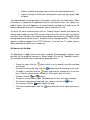
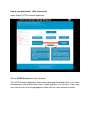
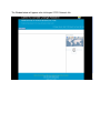
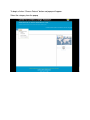
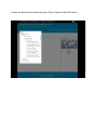
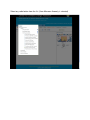
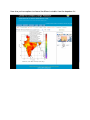
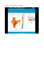
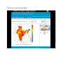
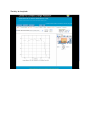
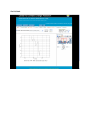
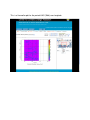
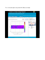
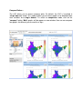
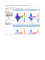
CCCR Outreach FAQ and User Manual
Q.1 What is the CCCR Outreach Application used for?
The CCCR Outreach Application is a Web interface for displaying data. The
CCCR Outreach Application Access enables you to:
-
Display maps, diagrams and graphs in color,
Request data to be extracted from the datasets in several different formats,
(This function is disable)
Compare different plots over different year and calculate the difference between
any four years.
Animation for the particular period available on every datasets.
Calculate basic statistics (such as average, sum, maximum, minimum and
variance etc.).
Q.2 How to use the CCCR Outreach Application and minimum requirements to
run it?
1. Best viewed on Mozilla Firefox 3.5+ (Download from Here)
2. Activate the 'pop up' option in your web browser to enable graphic output. This
may not work correctly if pop-ups are blocked.
3. Set your browser preferences to enable Java and JavaScript
4. Requires cookies to be set to keep track of previous plot and subset choices
CCCR Outreach Application DOES NOT use persistent cookies -- that is, cookies
are NOT SAVED on a user's disk.
5. The cookie is only valid while a user's browser is active.
6. If this Application is not working for you, please check to make sure that Java
and JavaScript are enabled in browser and not blocking pop-ups. If the interface
still doesn't work, please contact us. (mailto : [email protected],
[email protected] , cc : [email protected] )
Q.3 What are the functions of this application?
This section describes the graphical interface and the main functions of the
CCCR Outreach Application. The following operations can be performed:
•
•
•
Select a dataset from category list by clicking “choose dataset” ,
Select a variable from this dataset,
Display Maps, Graphs in color, Line Plots and Hovmoller Plot.
•
•
Choose a spatial or temporal sub-set within the selected dimensions,
Choose the way in which data is displayed or retrieved: map, graph, table
of figures
You should perform these operations in the order in which they are listed above. When
this process is completed, the application delivers the desired results. For a graph or a
table of figures, the result appears in an internet browser window. In all other cases, the
browser downloads the results and prompts you to store them as a file.
To return, for more selection either click on “Choose Dataset” button and choose the
dataset and variable you want OR you can also click on this link to return to previous
selection. After Clicking on the Choose Dataset button the dataset list will popup. Select
the required dataset for the analysis. Keeping track of selected variables - The function
appears on different pages in the CCCR Outreach. If you click on “i” symbol, you can
obtain detailed information on a variable, etc.
Q.4 How to Use the Map
The Map doesn’t support unless Javascript is enabled. The geographic selection is only
possible via the graphical interface as shown below. Click on the "Maphelp" button if
you encounter any difficulty in selecting the geographic area.
•
•
•
•
•
•
•
•
To pan the map, click the
button (which is on by default) and click and drag
on the map.
To select an area of the map, click the
button then click and drag on the map.
To modify a selection click the
button and click the selected area (it will turn
blue). Drag the orange circles to modify it. (Click again when finished).
To zoom, click on
and
buttons.
To zoom in to a particular region, hold down the shift key, then click and drag.
To re-center and zoom out and keep your selection click on the
button.
To start over, click the
button above the map.
To select a named region, click the
button and click on the region you want to
select.
How to use Application? (With screenshot)
Home Page of CCCR Outreach Application
Click on CCCR Outreach link from left panel
The CCCR Outreach Application allows you to download (Download facility is the future
enhancement) and visualize data using a simple graphical user interface. It frees data
users from the hassle of writing programs to deal with the native format of the data.
The Window below will appear after clicking on CCCR Outreach link
To begin, click on “Choose Dataset” button and popup will appear.
Select the category from the popup
After clicking on Rainfall Dataset (Out of Four Category here you can select as per
requirement) the pop will appear.
Choose the dataset and variable you want, Click on Seasonal Rainfall Dataset.
Select any radio button from the list. (Here Monsoon Anomaly is selected)
Map will appear on the screen.
We can choose Maps, Line Plots and Hovmoller Plot. Map is 2-Dimensional (Longitude
and Latitude required), Line Plots have the Time Series, Longitude and Latitude.
Hovmoller graphs (also known as Hofmuller Plot) are a 2-dimensional plot showing how
the value of some quantity varies in space-time; one axis refers to time and the other to
spatial location. For example "MAPS (latitude-longitude)" gives spatial gridded or plotted
values at a specified time, "LINE PLOTS" gives a time series at a spatial point, and
"HOVMOLLER PLOTS" gives you a plot or extract the temperatures for a space and
time range.
Here also you have options to choose the different variables from the dropdown list
Similarly, we can choose different time period.
Click on Apply Analysis Button, a window will appear below
1. Choose different seasons Winter, Pre Monsoon, Monsoon and Post Monsoon from
Dropdown List
2. The "Start Date" and “End Date” parameter enables you to choose the date or
the period for the selected data you want to display.
3. Chose the Analysis Type and Region Type from Analysis dropdown list.
Here, A window will appear for the Analysis for different time period over the time,
longitude, latitude and area.
See the next screen for more details.
For the Time Series click on the Time Series radio button from above panel. This is the
time series plot for the period 1951-2008 (This is a just an example to understand the
analysis)
Similarly for longitude
And lattitude
This is a Hovmoller plot for the period JJAS (1988) over longitude
This is a Hovmoller plot for the period JJAS (1988) over latitude.
We can set plot options of colour bar using “Set Plot Option” Button.
Following window will appear.
Any of these parameters can be adjusted. Click on the symbol “i” to obtain more
information on each option.
1. Evaluate expression and Interpolate normal to plot
These determine the way in which the data are calculated and extracted from the
dataset. They are: "Evaluate expression", "Interpolate data".
- Expressing a new variable
The LAS enables you to define a new variable based on another variable which
already exists. In particular, this enables you to convert units.
For example: conversion of temperature from °C to °F. The expression is as
follows:
"Evaluate expression = 9.0 * $ / 5.0 + 32.0" The existing variable is represented
by the $ symbol.
- Data interpolation
By default, the LAS is installed with Ferret as its analysis and graphic engine.
Ferret enables you to interpolate gridded data from the original grid onto another grid.
By default, this function is disabled ("No").
If you select a value on an axis which does not correspond to the position of a
grid point, Ferret will use the nearest grid point on this axis to generate the requested
product. You can activate the interpolation function from the "Output Options" page;
Ferret will then use the linear interpolation method to calculate the data for the exact
points you have chosen.
If you wish to enable the data interpolation function, select "Yes" in the
"Interpolate data" option.
For example: The LAS has used the interpolation function to calculate a gridded
map at a depth.
The Ferret visualization tool enables gridded data to be interpolated from the
original grid onto another grid. For example, if you select a value on an axis which does
not correspond to the position of a grid point, Ferret will use the nearest grid point on
this axis to generate the requested product.
2. Image Format
The "Image format" option enables you to choose between GIF formats (pixilated
image)
Select Option, Default image format is GIF
3. Plot Size (Image Size)
The "Plot size" option gives a choice of three possible image sizes: Large,
Medium and Small
4. Choice of palette of colors:
This option enables you to choose the color scale for the graph. A wide choice of
palettes is available. The "Colour fill style" option gives a choice of possible fill
styles: Fill levels are described using Ferret syntax. The number of levels is
approximate, and may be changed as the algorithm rounds off the values.
Examples: (0, 100, 10) Bands of color starting at 0, ending at 100, with an
interval of 10. This parameter enables you to adjust the fill levels on the color
scale. It is based on a complex and powerful syntax (see "Ferret User Manual")
which allows all possible choices to be selected.
For example: To obtain very detailed color variations around 0°C
for example every 2 degrees between -5 and 5 degrees; then less detailed for
more extreme values (every 5 degrees); and lastly, more distinction above + 45 or
below - 45 degrees (as far as the extreme values possible: either + or – 90), you
would select the
following:
Fill levels: (-90) (-45,-5, 5) (-5,5,2) (5,45,5) (90)
size
By default, the LAS use different colors in the map's background to represent the
variations displayed.
5. Choice of Contour Levels
You can also choose which contour lines to use, with the "Contour levels"
parameter.
This is based on the same syntax as the "Fill levels" parameter described earlier.
6. To Plot the trend
1. Margins - Make the plot with or without margins: when no margin is chosen,
the axes are at the edges of the plot (WMS-style plots). By default margins
are shown.
2. Degrees. Minute axis - Format the labels on plot axes that are in units of
degrees longitude or latitude as degrees, minutes rather than degrees and
decimal fractions of degrees. For axes with other units, this setting will be
ignored.
3. Trend Line - Overlay a trend line. For the option "Trend Line and Detrended",
a second panel is added, showing the variable minus mean and variable
minus mean and trend. Note that the slope of the trend is computed using the
units of the independent axis. A monthly axis may have underlying units of
days, so in such a case the slope will be data units/days.
4. Dependent Axis Scale - Set scale on the dependent axis lo, hi [, delta] where
[, delta] is optional, units are data units. If a delta is given, it will determine the
tic mark intervals. The dependent axis is the vertical axis for most plots; for
plots of a variable vs height or depth it is the horizontal axis. If the scale is not
set, Ferret determines this from the data.
Similar options can be set for the Animation using “Animate” Button.
Palette Style – Choose appropriate color from menu.
Time Step - Set the time step for animation. It is between 1 and the number of frames
being selected.
Contour Style - What style of contours to draw Choices are:
•
•
•
•
•
Default -- let LAS decide
Raster -- Fill each grid cell with the appropriate color
Color filled -- Fill in between contour lines with color
Lines -- Just draw lines
Raster and lines -- Fill in each grid cell and draw lines on top
•
Color filled and lines -- Fill in between contour lines with color and draw lines
on top
Match aspect ratio of plot to aspect ratio of region, Choices are
•
•
•
Default -- let LAS decide the aspect ratio
Yes -- Force LAS to calculate the aspect ratio of the plot based on the aspect
ratio of the geographic region
No -- Do not change the aspect ratio based on the region.
Land fill style - Style for drawing continents. Only applies to XY plots. Choices are:
•
•
•
•
Default -- let LAS decide
None -- don\'t draw continents
Outline -- draw continent outlines
Filled -- draw filled continents
Compare Button –
The LAS allows you to choose compare plots. By default, the LAS is launched in
"single data set" mode. This mode enables you to create graphs or to download data
from variables in a single dataset. To switch to comparison mode, click on the
"compare" button. Multi- graphs will be appear on new window, Here we can compare
four graphs for different year or months or days.
Difference mode between more than two years. (Up to 4 years)
Print Button –
We can save the image as GIF or can take print PDF or GIF.
Thank you