1
Research Papers
Issue RP0257
June 2015
Clime: climate data processing in
GIS environment
Regional Models and
geo-Hydrological Impacts
Division (REHMI)
By Luigi Cattaneo
Regional Models and
geo-Hydrological Impacts
Division, CMCC,
Via Maiorise s.n.c., I-81043,
Capua
[email protected]
Valeria Rillo
Regional Models and
geo-Hydrological Impacts
Division, CMCC,
Via Maiorise s.n.c., I-81043,
Capua
[email protected]
Maria Paola Manzi
Regional Models and
geo-Hydrological Impacts
Division, CMCC,
Via Maiorise s.n.c., I-81043,
Capua
[email protected]
Veronica Villani
Regional Models and
geo-Hydrological Impacts
Division, CMCC,
Via Maiorise s.n.c., I-81043,
Capua
[email protected]
and Paola Mercogliano
Italian Aerospace Research
Centre (CIRA)
Regional Models and
geo-Hydrological Impacts
Division, CMCC
[email protected]
The work here presented
has been carried out in
close cooperation
with dr. Francesco
Cotroneo
SUMMARY Clime is an extension software for ArcMap 10 environment
featuring multiple tools for observed and simulated climate data analysis.
Since a large number of functionalities is featured in Clime, this report has
been intended as an introductive guide for any user which could be
interested on its practical purposes. Due to its nature, a background
knowledge of ArcGIS software is required. The paper is structured as
follows: section 1 (Introduction) briefly explains the reasons who brought to
software development, along to its general purposes; section 2 is an overall
description of software internal architecture; section 3 deals about all data
import and managing processes to run before analysis; in section 4,
database connection settings are described; section 5 shows all processes
involving output image rendering, like plots and maps; section 6 explains
Bias Correction tools; section 7 is about homogenization of station data;
finally, section 8 describes all remaining processes, dealing primarily on
graphic interpolation and format conversion.
Keywords: Climate Data Analysis, Geographic Information Systems
CMCC Research Papers
1 INTRODUCTION
Centro Euro-Mediterraneo sui Cambiamenti Climatici
02
REMHI-Capua division had several collaboration experiences with impact communities, including European Projects, such as IS-ENES
(VII FP - Infrastructure 2008)[2], SafeLand(VII
FP - Environment 2008), about the study of
landslide risk in Europe, ORIENTGATE (South
East Europe Transnational Cooperation Programme 2012), and finally INTACT (VII FP , Infrastructure 2013). These partnerships brought
to the execution of different reseach activities
concerning the quantitative analysis of the various impacts of climate change which are mostly
based on the use of high and very high resolution regional climate models. The CMCCREMHI division also collaborates with local institutions interested in climate change impacts
on the soil, such as river basin authorities in the
Campania region, ARPA Emilia Romagna and
ARPA Calabria. Hence Clime, a Geographic
Information System (G.I.S.) developed add-in
tool, is the result of such close collaboration
with impact communities with the main goal to
grant the use of climate data also to users with
little experience in this field. It features a reliable interface allowing to easily manage climate
data and evaluate their reliability over any geographical entity of interest, by accepting multiple sources of different formats, like observations and/or numeric model outputs, and using
them as inputs for traditional models (hydrologic, slope stability, etc.). The latter feature is
of particular interest for different end users because spatial resolution of modern regional climate models (e.g. COSMO-CLM, MM5, WRF
Model) is currently of about 10 km, which is too
poor for impact studies or other activities - which
may involve civil protection, cultural heritages,
historical studies of impact in limited areas - that
need input data at a resolution of about 100 meters. For this reason climate data are usually
processed with any of the downscaling meth-
ods provided by literature. It is clear that downscaling approach represents a crucial research
activity in order to extend the application field
for high resolution climate models. The main
focus of research in this last field is to improve
downscaling processes in order to have them
grant high standards of technical performances
and reliability. Plus, the identified dowsncaling
method is expected be implemented through a
fast algorithm without high hardware requirements: once it is finally selected,it is necessary to perform an extensive validation of its
results produced by comparing them with time
series collected from weather stations, radars
and satellite data. Comparison of an usually
large number of permutations, along with the
processes for data homologation, requires automated and generalized procedures that must
also be equipped with interfaces to link them
into the operating pipeline. All these needs
have brought to the development of the CMCC
Clime software, which provides several methods for post-processing and validation functionalities, featuring the above described interoperability. Assuming that the base structure of a
GIS is characterized by a set of layers in vector or raster format (collimating square cells)
where any climate model and dataset could
be easily stored, Clime has been implemented
as an extension for ESRI ArcGIS Desktop and
is launched from a plugin user interface (bar
anchored to the main toolbar), allowing users
to take full advantage of the high level primitives (e.g. block functions for interpolation, algebra on raster, reference systems transformations) and many other features provided by the
base software: as a result, this combined array of processes is expected to cover all the
steps concerning the phases of validation and
data processing. Finally, analysis results are
displayable in a variety of formats and standards with any assignment of classifications,
histograms, and legends.
Clime: climate data processing in GIS environment
Clime is classified, by its nature of extension,
as a special purpose GIS software integrated
in the consolidated and evolved ESRI ArcGIS
Desktop 10.X, thus providing in this mode a
dynamic linkage library (DLL) that is compatible with Microsoft Windows operating systems
(all versions NT-compliant) and functions provided by ArcGIS Desktop. As shown in Figure 5,
Clime tightly integrates its graphical user interface (plugin mode) with the host system through
an anchored bar with function buttons, each
one related to a distinctive feature of the software. Besides, it is designed to act mostly as a
stand-alone utility, in order to meet easy portability requirements: the implementation of his
algorithms has been coded separately from the
GIS portions, for which routine calls to the native environment are used. On a closer look,
Clime operates on an internal database (powered by Microsoft Access RDBMS) which can
be accessed only through a SQL 9.2 declarative language, linked to a catalog dedicated on
tracking any task to be carried out and its processed data in order to historicize the associations between methods and validations, as well
as suitably mark the import data as a function of
the source specific data. The development language used is a subset of C#.NET compatible
with the MONO framework, whereas the parts
concerning the primitive GIS are native libraries
that are accessed through the ArcGIS API ArcObjects and ArcToolbox. The chosen approach
has noticeable advantages: the C# language
independently manages the dynamic allocation
of memory, and calculations with heavier computational load are executed by native modules, which grants faster performances. The
execution speed is a key requirement for this
type of product: the validation phase may imply the production of a large amount of data
(small-scale forecast models with dense tem-
poral sampling, time series of weather stations,
radars or satellites), expected to be processed
with multiple methods of downscaling; then, the
production phase requires to provide forecasts
in nearly real time, to fit cases like emergency
management. At the present moment, Clime requires the support of ESRI ArcGIS Desktop 10.X
(an ArcView license is sufficient), with Spatial Analyst extension, but its structure makes it open
to further solutions. In fact, another advantage of the choice of C# language MONO is the
complete portability of the code (as well as the
forms) - in detail, any part not directly interacting with ArcGIS - in all major hardware platforms
and software (Unix-like, MacOS, X86, SPARC). In
this way, the real porting issues are expressly
limited to the GIS modules (geo-processing,
map algebra, spatial interpolation, reference
systems), but all these components are well
documented and their reimplementation is not
strictly necessary, since there is the possibility
to use business forms and many available Open
Source codes. The described operations could
either keep the original Clime layout, intended
as a mere extension (e.g. with multiplatform
as QGIS or GRASS), or simply provide it with a
stand-alone execution mode.
3 EDITING PHASE: CLIME DATA
MANAGER
Clime is conceived to handle data with specific
features, so it is necessary to build and arrange
data in a suitable way. Such pre-processing
phase is carried out by Clime Data Manager (Figure 1) a database interface which allows to import new data and to edit existing ones. This
software is executed separately and does not
need any environment application. Data are
stored as layers. Afterwards, it is possible to run
any desired process with the main software. In
the upper part, it is possible to manage all previously stored layers by selecting the database
03
Centro Euro-Mediterraneo sui Cambiamenti Climatici
2 SOFTWARE ARCHITECTURE
CMCC Research Papers
Centro Euro-Mediterraneo sui Cambiamenti Climatici
04
through the Server address box and searching
the requested data by filtering results selecting:
Grid type (numerical climate models as
COSMO-CLM [11], gridded observational
dataset as CRU [5][9])
Resolution (spatial resolution, in km)
Time aggregation (DAY, MONTH, YEAR,
SEASON)
Field (e.g. Temperature, Rainfall, Wind
speed)
Multiple choices are allowed (for example,
COSMO, 8 km, Temperature). It is also possible to filter results by name, selecting a part
or the whole name of the desired layer. Once
that the search criteria have been defined, it
takes to click on Refresh to visualize the requested layers. Then, he desired element is
selected by clicking on the gray square in the
leftmost column: in this way, the entire row will
be highlighted. The lower half part is dedicated
to three different processes: Import, Aggregate, and Export. It is also possible to filter results by selecting a keyword included in
the name of desired table: for instance, the
search can be focused on every object containing daily-aggregated temperature data with italy
in its name, with COSMO grid, 8 Km-resolution.
Once that all search criteria have been defined,
it takes to click on Refresh to visualize the requested layers. Then, the desired element is
selected by clicking on the gray square in the
leftmost column: in this way, the entire row will
be highlighted.
first step consists on identifying the original format of the input data and properly converting it
into a standard one: currently, managed data
are in Network Common Data Form (NetCDF) or
Comma-Separated Values (CSV) format and are
represented as discrete functions of space and
time. There are no particular constraints on the
shape of the physical domains, moreover values could either be distributed on a regular and
time-invariant grid (usually for model data), or
be spread on an erratic cluster of points (station
data), with setting nominal resolution as the average distance in kilometres between adjacent
points (-1.00 for irregular grids); concerning the
temporal evolution, it only takes to determine a
start date and a nominal step (e.g. hour, day,
month) between adjacent time units. Files containing data on a single time step (single maps)
and one-point datasets are also allowed. In order to properly run this process, overall structure of input files must be arranged as follows:
NetCDF
Files are required to have the following
fields:
longitude and latitude (one or twodimensional, -180◦ to 180◦ )
time (one-dimensional vector with integer values, must be named time)
specific
data
dimensional)
CSV
3.1 IMPORT
In order to process data in Clime, it is necessary to import the requested data into dedicate
database clusters (Figure 2). Hence, the very
Header
field(s)
(three-
Clime: climate data processing in GIS environment
Centro Euro-Mediterraneo sui Cambiamenti Climatici
05
Figure 1:
Clime Data Manager form. All functionalities are directly called through this menu.
Delimiter: ;
id stazione;lon;lat;<any
fields>;time ;shape
idx;idy;itime;lon;lat;<any
fields>;time ;shape
number
of
number
of
shape:
’SRID=3857;POINT(<Mercator
Sphere coordinates separated by space>)’
(ex.
’SRID=3857;POINT(1647529
7733594)’)
Examples
Types
id stazione: character string (max. 20)
idx, idy, itime: integer
lon, lat: real
data field: real (NaN allowed)
time : yyyy/MM/dd hh:mm:ssZ , leave Z
at the end (ex. 1970/01/01 00:00:00Z)
id stazione;lon;lat;hsurf;time ;shape
idx;idy;itime;lon;lat;tmin;tmax;time ;shape
The file (NetCDF or CSV) containing the data to
be imported can be selected from the file sys-
CMCC Research Papers
Centro Euro-Mediterraneo sui Cambiamenti Climatici
06
Figure 2:
Import section (Clime Data Manager)
tem by clicking on the button Select file. Then, it
is necessary to specify the following attributes:
Layer name: chosen by the user
Type: the variable considered (e.g. Temperature)
Name: the short name of the variable
(e.g. T 2M)
Unit measure: the desired Unit measure
e.g. K (for Kelvin degrees)
Transformation: if data in the original file
are in a different Unit measure from the
desired one, it is necessary to specify the
Transformation factor (e.g. K -> ◦ C if original data are in Kelvin degrees but are
requested to be in ◦ C degrees).
Partitioned option should be selected if a
large amount of data must be imported (e.g.
daily data over a 30-year period). During the
process, temporary CSV files are created in
a dump folder, whose path is chosen by the
user and has two different names: the one
directly related to destination device (Server
Dump Path), and the other as seen from user
machine (Local Dump Path, generally includes
an IP address); these paths are equal if data
is imported into the same device (localhost).
Finally, the import process can be started by
clicking on Import button and the related layer
is copied into the database selected in Server
address box.
3.2 AGGREGATE
Since data contain values characterized by a
regular time step (e.g. hour, day, month and so
on), it is also possible to create objects starting from existing ones by rearranging its content into a longer period through a set of aggregation functions (max, min, mean, standard
deviation, sum)(Figure 3). For instance, a table of monthly means could be obtained from
a dataset of daily values. Season aggregation
consists of four parts of year, each one com-
Clime: climate data processing in GIS environment
Figure 3:
Aggregate section (Clime Data Manager)
3.3 EXPORT
This functionality allows user to export a table
from any database to a local device, as a CSV
file (Figure 4). Once an object (Table name)
is selected, it is possible to choose the fields
to include into the output file (it is possible to
select all fields by clicking on the button Select
all and then to click on the button Export. Data
is always arranged by date and position, even
if these fields are not exported.
07
Figure 4:
Export section (Clime Data Manager)
set of processes, except for Get Point, which
enables an interactive mode with ArcMap environment and is assumed to co-operate with
other functions. At the beginning, the only one
active is Get Started, opening the login form
(Figure 6): user can edit the database list and
select the ones to connect to before logging in
for any ongoing process. Moreover, it is possible to choose the folder path where to save output raster objects. In order to properly run all
further operation, Climate should be selected
as Primary Mode. After setting these preferences, Clime session can be started through
CMCC-Clime button.
Figure 5:
Clime toolbar in ArcGIS Desktop 10 environment. Each
button calls a different form.
4 HOW TO START: CLIME LOGIN
Once ArcMap 10 is started, Clime toolbar can be
made visible by checking Clime - CMCC on
toolbar list (mouse right-click on screen), displaying multiple buttons (Figure 5), each one
related to a form characterized by its distinct
5 OVERHAUL & COMPARE
In Overhaul & Compare form (Figure 7), it is
possible to select the layers to be analyzed by
clicking the + button. In this way, the main
Centro Euro-Mediterraneo sui Cambiamenti Climatici
posed of three months (DJF, MAM, JJA and
SON); if True season option is enabled, December data is taken from the year preceding
January and February of the same block (DJF).
If input data contain monthly means, cumulative values can be evaluated (MonMean →
MonSum). It is worth to point that Clime is
capable of aggregation during processes, but
dealing with tinier tables helps users to save a
significant amount of time.
CMCC Research Papers
Centro Euro-Mediterraneo sui Cambiamenti Climatici
08
Figure 7:
Login and Settings form. User can choose databases and output folders here.
window form (Figure 8) will appear. Through
this window, every piece of data stored into selected databases is visible as layer in a list, each
column showing a different feature (name, category, grid resolution, time aggregation, etc.).
Once all preferences are chosen in the filtering box, it is possible to click on the Refresh
button and all search results are shown. After
selecting a single layer (the entire row will be
highlighted), it takes to click on the Add button
in order to add it to the process list. There is no
restriction on the number of layers, but it is important to notice that selection is limited to data
sharing a common period and the same time
aggregation (day, month, etc.). Looking into the
catalog form, each data unit is characterised by
a unique set of features and is representable as
a grid of geo-referenced points, either regular or
not, evolving on a discrete period (any number
of time steps). They can be easily viewed on
ArcGIS as layers. Back in Overhaul & Compare
form, it is possible to choose a space domain
(or point) from a list of reference areas - mostly
countries and continents, with a more specific
array for Italy - imported from GIS shape files,
and a time period (with season filter, if desired).
Then, a tab-arranged menu explains which operation could be run: usually, the output is ei-
Clime: climate data processing in GIS environment
Figure 6:
Login and Settings form. User can choose databases
and output folders here.
ther a plot chart or a map represented as a
layer/raster object on the GIS. All the options
are briefly explained in the following sections.
5.1 PLOTS
In this tab (lower part of the form show in Figure 7) it is possible to run any data analysis
displayable as line plots, mostly on a temporal
scale. Normally, input data are averaged over
the selected domain before undergoing further
operations. The graphic output is fully customizable by choosing colour, line width, pen
style, marker shape and label name for the legend through the Plot Settings window. Once
data are plotted, the user can customize it by
setting axes, labels and legend, and save it as
an image or Excel file.
5.1.1 GENERAL
This section display a set of functions mostly
used to analyse temporal trend of selected
data. A combo box menu allows user to choose
Time Series: this process displays the
data evolution through the reference period, with a time scale determined by the
user (e.g. days, months, years), so that
every plotted point is evaluated as temporal mean over the given time unit. Optionally, extreme values (max/min) and standard deviations are displayable, along
with the trend line (obtained with least
square method), which provides an idea
about the overall behavior of the data considered. Plus, choosing the Running
Mean option, the time series will be represented on annual scale, each value averaged on a selectable window of adjacent values (only odd integer ranges allowed). For example, choosing a window
with range 3 will produce for the year y0
the mean over the period [y0 − 1, y0 + 1]
(3 steps). Finally, in order to assess
the presence of a real trend in a dataset
within test period, a Mann-Kendall significance test could be performed. The alpha
threshold parameter is set to 0.05 by default, meaning that the normalised trend
rate must reside in the 5% tail of standard
cumulative distribution function (CDF) in
order to reject null hypothesis and have
H=1 (trend presence). It is important to
notice that such test has relevance as
time step of every processed dataset is
kept constant.
Seasonal Cycles: this function produces
a 12-steps plot, synthesizing values related to every distinct month.
More
clearly, the first value is the mean collected over all the ones belonging to Januarys, and so on. Also here it is possible
to evaluate extremes and standard devia-
09
Centro Euro-Mediterraneo sui Cambiamenti Climatici
one of the following processes (listed in Table
1):
CMCC Research Papers
Centro Euro-Mediterraneo sui Cambiamenti Climatici
10
Figure 8:
Catalog form, displaying all layers available for Clime processes.
tion; it works faster with already monthlyaggregated data.
PDF: the Probability Density Function is
obtained with counting the occurrences
within every bin interval, and then normalized by the total number of values
(discrete approach). Bin resolution is selectable, as well of total range of values,
but the latter could also be automatically
detected (overall minimum and maximum
are chosen in this case); Reject values allows to reject all values below selected threshold before building the PDF.
By checking Spatial Mean Values option,
input values are actually averaged over
the domain area for every time step (as
described before), otherwise all singlepoint values are processed.
Bias:
this process compares the sin-
gle layer selected in as Reference Layer
(lREF ) with all the other ones (ln ), calculating a point-by-point difference (ln −
lREF ). Thus, every plot contains the spatial mean of such difference (bias), represented at the selected time aggregation
(Trend option available).
Scatter Plot: this process compares two
datasets by placing their value domains
on the X-Y axes and drawing a point as result for every time step of the interval (e.g.
values x0 and y0 related to the same step
are mapped as point P(x0 , y0 ) ). Pearson
coefficient (correlation) can be evaluated
(it is equal to 1 if the two datasets are
the same), as well as covariance factor.
It is possible to plot a least-squares line
indicating the overall relation between the
two input datasets. Usual inputs are couples of arrays, like a modelled series and
Clime: climate data processing in GIS environment
Correlation: same as Time Series, but
used for plotting heterogeneous data with
different measure units (e.g. temperature
and rainfall). For a better comparison,
Pearson coefficient evaluation is available
in this case.
Verification Measures (only for daily rainfall): this process is conceived to compare
modeled data with the relative observed
dataset. Proceeding with a dichotomous
(yes-no) prediction, where each value is
compared in order to verify if it is equal
or greater than a determined threshold
(respectively 1,2,5,10 mm/day), the modeled values and the corresponding observations are represented in a contingency
table with the following responses: hit (the
event is both observed and predicted by
the model); false positive (the event is predicted by the model but not observed),
missed (the event is observed but not predicted by the model), correct negatives (the
event is not observed and not predicted by
the model). Then, key quality measures
in this system are defined as:
between the observed data and simulated results. Such score is computed in the Elaboration Form.
{ POD (Probability of Detection): percentage of observed events correctly modeled.
{ FAR (False Alarm Ratio): percentage of events predicted by the model
and that do not verify.
{ CSI (Critical Success Index): percentage of observed and/or modeled values that were correctly predicted.
For each index, a chart is plotted with values
corresponding to distinct thresholds.
5.1.2 ERRORS
In this section (Figure 9), Clime analyses the
differences between a set of objects and a Reference Layer and displays the results as error
indices listed in Table 2. By checking Process
all seasons, it is possible to perform such process for every single season (total: 4 runs).
There are two main modes to run processes:
{ PC (Proportion correct): measures
the model accuracy by considering the simple matching coefficient
based on the ”proportion” of total
”correct” hits and rejections.
Calculate Indices: selecting this option,
software first evaluates spatial mean of
every element, then performs index evaluation which may involve comparison between two layers. At the end of process,
all indices are shown on a table.
{ BIAS: percentage of events modeled to those observed, and should
be unity (unbiased) for a perfect system. In practice, it generally differs from unity due to the presence
of systematic biases (errors) in the
model or observing system. From a
climatological point of view, bias is
defined as the systematic difference
Draw Taylor Diagram: Taylor Diagram is
a quick way of comparing the behaviour
of multiple datasets with respect to a reference one [13]. All datasets (including
the reference one) are represented as
points inside a circle, being their radial
distance proportional to the standard deviation. The reference point is located
on the abscissa axis. The distance of
11
Centro Euro-Mediterraneo sui Cambiamenti Climatici
an observational dataset.
CMCC Research Papers
Table 1
Centro Euro-Mediterraneo sui Cambiamenti Climatici
12
Complete list of plots and their related available options
Min/Max
St.Dev.
Least Sq.
Correlation
Covariance
Run.Mean
Mann-Kendall
Time Series
Yes
Yes
Yes
No
No
Yes
Yes
Seasonal Cycles
Yes
Yes
No
No
No
No
No
PDF
No
No
No
No
No
No
No
Bias
No
No
Yes
No
No
No
No
Scatter Plot
No
No
Yes
Yes
Yes
No
No
Correlation
Yes
Yes
Yes
Yes
No
Yes
No
Verif. Meas.
No
No
No
No
No
No
No
each point from the reference one measures the centred root mean square error
(CRMS); correlation depends on the angle and varies as cosine. The diagram
is in normalised form and all distances
are divided by the reference standard deviation, so the reference point always is
always located in (1, 0).
Plus, the following options are available:
Characterisation: Indices are evaluated (by default) starting from spatial
means of each dataset (temporal diagram); choosing spatial diagram it is
possible to perform time mean instead.
The latter option requires all layers to
have the same grid.
Enable layer correction: a correction
layer (SINGLE MAP only) is added to all
elements, except for reference layer, before statistical processing.
5.1.3 INDICES
The following section deals with the index evaluation (Figure 10). Rather than displaying a sim-
Figure 9:
Errors menu
ple trend, it allows to aggregate data on monthly
or annual scale using a set of operators and
assuming conditions for every temporal tier. All
aggregate functions are listed below:
Mean/Min/Max:
age/minimum/maximum
the base period
value
averwithin
Sum: sum of values within the base period
Count: number of time steps within the
base period (where chosen condition occurs)
Clime: climate data processing in GIS environment
Mean
Variance
Covariance
Standard deviation
Correlation
µ=
PN
1
N
2 =
σX
n=1
1
N
Xn
PN
n=1 (Xn
− µX ) 2
1 PN
2
σXY
= N
n=1 [(Xn − µX )(Yn − µY )]
q
2
σX = σX
ρXY =
2
σXY
σX σY
Bias
BIAS =
1
N
PN
− Yn )
Mean Absolute Error
M AE =
1
N
PN
|Xn − Yn |
Root Mean Square Error
Centred Root Mean Square Error
n=1 (Xn
n=1
RM SE =
q
1
N
PN
− Y n )2
CRM S =
q
1
N
PN
− µX ) − (Yn − µY )]2
If requested, the process can be limited only
to a particular period or season of the year.
Month selection allows determining the months
to be observed. Input data is treated according to Monthly base settings, which produces
monthly values. Then, if the user chooses to
aggregate by year (lower-left option box), data
are ready to be processed by Yearly base operator. A spatial mean is performed in order
to have output represented on time plot. In
this way, it is possible to analyse critical events
within a chosen period by evaluating their ex-
n=1 (Xn
n=1 [(Xn
treme values and occurrence rate.
Example: starting from a dataset of daily
rainfall data, the requested output is the
total number of days per year with a precipitation amount exceeding 1 mm/day.
1. From Monthly base box, select
count and set value constraints to
≥1
2. From Yearly base box, select sum
3. Aggregate by year and plot
5.1.4 PLOT FORM
Figure 10:
All statistic operators evaluated by Errors with their
implementation
At the end of process, Clime displays a form for
every selected area, each one displaying results through a chart, as shown in Figure 11.
It is possible to regulate the scale interval and
the tick size of both the axes. The label format
can be properly customized with Label Settings
menu; legend could be moved, or even hidden. Finally, plot image can be exported as
13
Centro Euro-Mediterraneo sui Cambiamenti Climatici
Table 2
Complete list of statistic operators evaluated by Errors with their implementation
CMCC Research Papers
Centro Euro-Mediterraneo sui Cambiamenti Climatici
14
image (file.bmp) or excel table (file.xlsx). Some
examples of output images are shown below in
Figures 12-13-14.
Clime: climate data processing in GIS environment
Figure 11:
Sample Plot form with Time Series. The window is named after plot domain area.
Figure 12:
PDF sample
Figure 13:
Scatter Plot sample
Figure 14:
Taylor Diagram sample
Centro Euro-Mediterraneo sui Cambiamenti Climatici
15
CMCC Research Papers
5.2 ELABORATIONS
Centro Euro-Mediterraneo sui Cambiamenti Climatici
16
This macro-section (form shown in Figure 13)
includes all processes which produce graphical outputs (point feature or raster) which are
all available in the Table Of Contents window, while their source file is saved at the
path chosen during Start options. All maps
are geo-referenced with the projected system
WGS 1984 Web Mercator (Auxiliary Sphere). The
output map can be obtained from a single layer
or can be the result of a difference between
mapn and mapREF : mapn (test map) is related
to any object from the input layer list, while
mapREF (reference map) is the one selected
from the Reference Layer box. A difference
output always originates raster objects. Layer
differences can be evaluated in two different
ways (specified in Difference Representation box): simple difference mapn − mapREF
and percentage ((mapn −mapREF )/mapREF )∗
100.
Options
Create Raster: by selecting this option,
every grid point is turned into a raster
through an interpolation process (Natural
Neighbour, provided by ArcMap system
toolboxes). Algebra operations can be
performed only between rasters, so this
step always takes place before any subtraction to execute in case of differences.
Since the raster basic unit is a square,
its size is defined by input parameter Cell
Size.
Contour: this option allows executing
Contour With Barriers toolbox, creating a
feature layer with contour lines following
values of output map. The user may
choose contour interval.
The complete list of functions is showed below:
Figure 15:
Elaborations section, with Seasonal Differences menu
Seasonal Differences: this process (Figure 15) produces simple difference maps
evaluated within one or more distinct seasons. Each input dataset is filtered by
seasons before performing a time mean
over the selected period on every point of
the grid. If Enable layer correction option is enabled, an additional layer (SINGLE MAP only) is taken into account as
layer correction map (mapLC ) and therefore added to the test map in order to
have map′n = mapn + mapLC . It is useful
for example in order to perform a temperature elevation correction (related to the
orography).
Extreme indices: this section (Figure 16)
provides some basic tools to calculate extreme indices by aggregating input data.
It is either possible to select indices from a
default set taken from ETCCDI list, as displayed in Table 3, or to define a custom
version (Custom index). By selecting
this option, another form appears (Figure
17). As for Indices from Plot menu, the
user can choose aggregation operator for
every time base (month, year, total) or the
single months to analyse through Month
selection. Index name will be the same of
the field in output layer.
Clime: climate data processing in GIS environment
Index name
Frost Days (FD)
Ice Days (ID)
Summer Days (SU)
Tropical Nights (TR)
Hot Waves (HW)
Simple Daily Intensity Index (SDII)
Number of Heavy Precipitation Days (R10)
Number of Very Heavy Precipitation Days (R20)
Consecutive Dry Days (CDD)
Consecutive Wet Days (CWD)
Annual Total Wet-Day Precipitation (Prcp. Tot)
Figure 16:
Extreme Indices menu. Available indices vary depending
on selected input data (temperature or precipitation).
Definition
Number of Days/Year with Tmin < 0◦ C*
Number of Days/Year with Tmax < 0◦ C*
Number of Days/Year with Tmax > 25◦ C*
Number of Days/Year with Tmin > 20◦ C*
Number of Days/Year with Tmax > 35◦ C*
Daily Precipitation Mean during Wet Days (prec. >= 1mm)
Number of Days/Year with prec. >= 10mm*
Number of Days/Year with prec. >= 20mm*
Largest number of consecutive days with prec. < 1mm
Largest number of consecutive days with prec. >= 1mm
Annual Precipitation during Wet Days (prec. >= 1mm)*
aries, percentile evaluation is confined
within the chosen interval, with all other
values being completely ignored from
statistic count. Station check is an additional control to activate in case input
layers do not present values at every time
step (missing data), which frequently happens for station data. Since such option
comes at a higher computational cost, it
is recommended to enable it only if necessary. If desired, it is also possible to
enable the option to evaluate percentile
differences from reference layer.
Figure 17:
Custom Index menu
Percentiles: this section (Figure 18)
allows the calculation of different percentiles, which can be selected by choosing one or more threshold values (%).
Percentiles over the selected period are
evaluated in every point, in order to build
percentile maps. A single input object
produces one layer for each chosen percentile. By setting upper/lower bound-
Figure 18:
Percentiles menu. Multiple thresholds could within a
single process.
Trend tests: in this section (Figure 19),
it is possible to run trend tests on every point of the input layers and show
their results on the map. Currently, the
only test available is Mann-Kendall (see
17
Centro Euro-Mediterraneo sui Cambiamenti Climatici
Table 3
List of ETCCDI extreme indices provided by Clime (webpage: http://etccdi.pacificclimate.org/list 27 indices.shtml). (*) For periods
longer than one year, output map displays annual mean of index value
CMCC Research Papers
Centro Euro-Mediterraneo sui Cambiamenti Climatici
18
Plots): since it is meant to analyse annual
trends, all dataset are averaged by year
before being processed. Selecting Run
Test, data undergoes also spatial mean
and results are displayed as synthetic indices on a window at the end of process.
With Add result grid, test is performed on
every point of input layer, in order to return a map of responses (p-values and
hypothesis).
evaluated on temporal means and thus
layered on point grids. Since these operations require a point-to-point comparison,
only objects with similar grids are allowed
to this process. If a perfect match is not
reached, it is possible to set a tolerance
level (lon/lat round), though it is always
recommended to have grids of the same
resolution. Each output layer includes all
indices related to a single input dataset
mapn , compared with mapREF ; if desired,
layer correction is applicable.
Figure 19:
Trend Tests menu.
Differences: this process (Figure 20) produces simple difference maps evaluated
in a similar way as Seasonal Differences,
but in this case the user has to choose
test layers from the list in this tab, along
with a new time period, whereas the reference layer is unchanged. Such process is
often used to compare datasets focused
on two different time periods (e.g. future
minus past).
Figure 20:
Trend Tests menu.
Errors: this section (Figure 21) consists
on the same set of functions in Plot → Errors (see par. 5.1.2), except for they are
Figure 21:
Errors menu, for point-to-point layer comparing.
Figure 22 shows typical output maps rendered
through ArcMap interface and saved as image
files.
6 BIAS CORRECTION
Since modeled data may present unacceptable
bias values for impact studies, it is required to
carry out further controls and improve the reliability of predicted values. For this purpose,
a Bias Correction process generally involves a
comparison between model output and an observational dataset in order to evaluate the bias
rate and estimate correction parameters to be
applied on the whole modelled stream. More
specifically, Clime allows the user to run such
process on any test layer from the database
and create a bias-corrected new one (it is saved
into the database where station data is stored).
The process can be started by clicking on the
Clime: climate data processing in GIS environment
Figure 22:
Examples of indices maps. (a) number of weak precipitation days (d/yr) provided by EURO4M-APGD data, bias of weak
precipitation days of (b) COSMO-CLM0.0715◦ and (c) COSMO-CLM 0.125◦ versus EURO4M-APGD data. (d) number of intense
precipitation days (d/yr) provided by EURO4M-APGD data, bias of intense precipitation days of (e) COSMO-CLM 0.0715◦ and (f)
COSMO-CLM 0.125◦ versus EURO4M-APGD data [10].
button Bias Correction tool in the multiple buttons bar shown in Figure 5. The panel shown
in Figure 23 will appear.
The general process consists in comparing
Model Grid (Control) and Observation
Grid within Control Time period over the
selected domain, in order to create a correction mask, which is applied to Projected Grid
within the Projection Time interval, and evaluate a corrected grid whose values are saved
into an Output Table. First, it is necessary
to select the reference station point: with Add
Layers, both model and observation grids appear on the screen, then the Get a Point function from Clime toolbar enables user to choose
a given point by mouse click (Figure 24), whose
position is registered and used to evaluate the
nearest point relative to every grid under exam
(<<Set Nearest>>). Since the process takes into
account other points surrounding the reference
ones within a square neighbourhood, the user
must determine the size of such area (by de-
fault, it is a square with a 5-points side). Finally,
it is possible to choose the algorithm to use for
the bias correction (Quantile Mapping and
Linear Scaling, each one with its own settings).
6.1 LINEAR SCALING
This method consists in correcting the daily series starting from monthly values. For all the 12
months, the ratio between simulated and observed values is evaluated and then applied to
the input series as a correction factor [14]. It is
possible to run a process in cross-validation
mode, in order to have a correction mask applied to the same model dataset used to create
it. Anyway, this stage is just for performance
evaluation purposes and not strictly required.
As shown on Figure 23, two distinct algorithms
are available to evaluate and apply a correction
mask: Additive (1) and Multiplicative (2).
The mask is a gridded layer evaluated from the
i
means of observations VOBS
and model data
Centro Euro-Mediterraneo sui Cambiamenti Climatici
19
CMCC Research Papers
Centro Euro-Mediterraneo sui Cambiamenti Climatici
20
Figure 23:
Bias Correction form, with Linear Scaling process menu.
i
VRCM
, each related to a single month of the
year, collected over the entire time period. In
i
this way, every value of input grid VRCM
is subject to a correction depending on its position
and the month it belongs to, in order to obtain a
i
table of corrected values VCORR
. Output is generated on a square grid of the same dimension
and position of the one defined as the reference
station neighbourhood.
i
i
i
i
− VRCM
)
VCORR
= VRCM
+ (VOBS
i
i
VCORR
= VRCM
∗
i
VOBS
i
VRCM
(1)
(2)
6.2 QUANTILE MAPPING
Differently from previous case, this process
compares datasets by focusing on their statistical characterization. Given a modeled variable
Vm and an observed one Vo , their relationship
can be expressed through the transformation
operator h in the following way:
Vo = h(Vm )
(3)
Given that the distribution of modeled variable
is known, the latter equation could be displayed
as follows:
Vo = Fo−1 (Fm (Vm ))
(4)
Where Fm is the CDF related to Vm and Fo−1 is
the inverse CDF (also defined as quantile function) of Vo [4]. Since there are several ways to
approximate quantile function, user is allowed
to choose among a wide range of algorithms [3].
More specifically, this process (Figure 25) compares a selected station with a spatial mean
of the surrounding square grid, so only singlepoint grids are produced as output. Currently,
the whole process is focused on one manually
chosen station point, so only single-point grids
are produced as output. Some algorithms belonging to this class may require a parameter
to set the step of quantile probability vector (Q
Step), so user can choose it to have a default
(inverse of Vm length) or custom value(between
0 and 1).
Clime: climate data processing in GIS environment
Figure 24:
Coordinates selection using Get Point operator.
Figure 25:
Quantile Mapping process menu.
between the series under study (candidate) and
a number of reference series. These last ones
are a representative series of the climate of
the region in which the candidate gauge station
is located, and at the same time without nonhomogeneities. The process can be invoked by
selecting Homogenise function from Clime toolbar (Figure 5): the panel shown in Figure 26
will show up.
7 HOMOGENISE
The study of climate variability and the evaluation of climate tendencies require the availability of long homogeneous series of climatic
data. A time series is homogenous if variations can be attributed only to climate factors
[1]. Real data series are usually affected by
perturbations (or non-homogeneities) due to
external non-climatic factors. The time step
in which a series starts to exhibit a perturbation is usually defined as breakpoint (or changepoint). The information availability (metadata)
that supports the history of gauge stations simplifies the study of non-homogeneities in a time
series, so, in order to identify not documented
non-homogeneities and to correct their effect
on the series, several methodologies have been
developed, mainly statistical (homogenisation
methods). Most of the widely used statistical
methodologies are based on the comparison
7.1 DATA INPUT & OUTLIER
RESEARCH
This functionality is used on station data in
order to check the presence of abnormal values among observations (outliers), whose high
number may affect predictions and alter their
statistic distributions, thus leading to a faulty
estimation. In the upper part of the panel, it is
possible to search the requested layer by using
searching criteria based on Grid Type, Resolution, Time Aggregation, Field and clicking on
Refresh button. Then, the selected layer is visualised as an ArcGIS layer through the Add layer
button. The test is carried out on a single station point selected with Get a Point button and
elected as candidate. The exact position which
is needed for the process execution is obtained
by clicking on the Set nearest button. The reference stations are determined according with
Centro Euro-Mediterraneo sui Cambiamenti Climatici
21
CMCC Research Papers
Centro Euro-Mediterraneo sui Cambiamenti Climatici
22
Figure 26:
Homogenise form, including both catalog view and process options.
the following parameters:
Maximum distance from the candidate
station;
Maximum and minimum number of reference stations to be determined;
Minimum correlation value with respect to
the candidate station.
Outlier percentile for multi-station method
(95% or above recommended, especially
for daily data)
Each reference point series must first pass a
completeness test, in order to ensure it contains a satisfying percentage of valid data (at
least 75%), with results shown in the file Table.txt (1 indicates a positive response, 0 a
negative response). In the case of rainfall data,
negatives are corrected to null and 4-days (or
longer) streaks of non-zero constant values are
considered as a suspicious behaviour. If data
are sufficient, the quality control is performed.
The result is expressed through iQuaSI coefficient, evaluated with the following formula:
LA
LB
LC
) + bL × (
) + cL × (
)
L
L
L
LD
(bL + cL )
LN A
+dL × (
)+(
)×(
)
L
2
L
(5)
iQuaSI = aL × (
where coefficient values [aL , bL , cL , dL ] are defined by data class and series length L, as
listed in Errore. L’origine riferimento non è stata
trovata., and ratios Li /L are relative to the percentage of metadata belonging to a single quality class i over total period L (n◦ of years ). Each
quality class is defined as a function of the available metadata:
Class A: data measured with high accuracy instrumentation (< 3%) (e.g. electronic recorder rain gauge in perfect efficiency)
Class B: data measured with medium accuracy instrumentation (3-5%) (e.g. mechanical recorder rain gauge)
Clime: climate data processing in GIS environment
Data class
L ≥ 30
A
B
C
D
Series lenght
15 ≤ L ≤ 30
5 ≤ L ≤ 15
1
3/4
1/2
0
Table 5
Correspondence between quality rate and iQuaSI
Quality
iQuaSI
HIGH
GOOD
SUFFICIENT
POOR
BAD/UNUSABLE
0.9 < iQuaSI ≤ 1
0.7 < iQuaSI ≤ 0.9
0.3 < iQuaSI ≤ 0.7
0.1 < iQuaSI ≤ 0.3
0 < iQuaSI ≤ 0.3
Class C: data measured with low accuracy instrumentation (> 5%) or estimated
through indirect variables (e.g. simple
rain gauge, meteo radar for precipitation,
flow rate estimated through discharge
scale).
Class D: missing data, or reconstructed by
mathematical modeling.
If metadata are not available, an average value
between quality coefficients bL and cL is attributed by default. IQuaSi index ranges between 0 and 1 and provides information about
the series quality, according to the five intervals
shown in table [6]. Only datasets with overall
quality SUFFICIENT or above are considered
valid reference stations.
Such control is carried out starting from the
closest reference point, until it collects a sufficient number (defined by the user) of stations
fulfilling this criteria; if a minimum number is
not reached, the process is aborted. Once all
reference stations are gathered, the candidate
3/4
1/2
1/4
0
1/2
1/4
0
0
L≤5
0
0
0
0
is scanned by means of three different algorithms (multi-station, quartile and mean-sd), in
order to identify any possible outlier. The multistation process is the only one using reference
stations, whereas others just focus on candidate. It is carried out only in case that three or
more reference stations are found, otherwise it
is skipped. Each value from the candidate time
series is compared to all the related values belonging to the reference series, and is marked
as outlier if it is too from them. In this case, a
standardised value is evaluated and displayed
in the output text file. Such analysis is carried out separately for all the four seasons, but
results are listed together [7]. In the quartile
method, the 25◦ and 75◦ percentiles (respectively 1st and 3rd quartiles) are evaluated for
every season in order to define outliers, which
can be either moderate or extreme, depending
on their exceeding amount from such values [8].
The Mean-sd algorithm is so called because it
elects as outliers any value exceeding seasonal
mean by more than 3 times its standard deviation (sd)[12]. Finally, all results from the previous processes are then compared, and outliers
found by all the methods (common outliers) are
written into the output file, each represented as
a day-by-day list (in case of daily data).
The process generates the following files:
stationList.txt: list of reference stations
(position and table)
yyyy-MM-dd hh-mm Outliers.txt:
23
Centro Euro-Mediterraneo sui Cambiamenti Climatici
Table 4
Table of coefficients for quality control
CMCC Research Papers
Centro Euro-Mediterraneo sui Cambiamenti Climatici
24
list of outliers obtained with all the three
methods
yyyy-MM-dd hh-mm Table.txt:
completeness results
yyyy-MM-dd hh-mm BaseS.csv:
candidate data list
yyyy-MM-dd hh-mm RefS.csv:
correlation-weighted average of reference stations (if the number of reference
stations is lesser than three, it will not be
created)
Important: in order to correctly get the station
coordinates, only the selected grid must be visible on ArcGIS interface, so its related layer in
Table Of Contents should be left checked.
8 OTHER FUNCTIONS
Despite most features have been described in
previous sections, there are also other functionalities which interact with ArcGIS objects (layers,
rasters) and can be directly executed through
Clime toolbar buttons. Standard Interpolation function (Figure 29) basically reproduces
Interpolation toolboxes provided by ArcGIS with-
Figure 28:
Change Pars menu (pthr value is available only for daily
precipitation data).
7.2 BREAKPOINT TEST
Afterwards, it is possible to run the changepoint
test through the RHTestV4 software package
interface (it automatically appears at the end of
the process), which enables the user to edit
the various parameters used in the analysis
and apply a corrective algorithm to the data
series [15] [16] [17]; if input data is a daily
rainfall, a slightly different version is executed
(RHtests dlyPrcp). For a more detailed documentation on this software package, a complete guide is available [18]. If needed, the
parameters displayed in the main form (Figure
27) can be changed through the Change Pars
button (Figure 28). The current nominal level
of confidence (p.lev) must be chosen among
the following values: 0.75, 0.80, 0.90, 0.95,
0.99, 0.9999. In the case of daily precipitation
data, it is also possible to set the lower precipitation threshold to be considered in the process (pthr). Finally, Transform Data converts
daily data series in RClimDex standard format
to monthly mean series in RHtestsV4 standard
format.
out running them from Catalog window. More
precisely, available processes are: IDW, Natural Neighbour, Spline, Trend and Kriging. Since
the early development stage of this section,
there is still a limited operability: after user defines input data (e.g. t2m, tot prec), Clime picks
the first point feature of Table Of Contents having this field and interpolates it with selected
algorithm. As a future improvement, it would
be possible to select more grids in order to run
multiple interpolations at once. Import/Export
Figure 29:
Standard Interpolation form.
tool (Figure 30) is conceived to handle output
raster maps, both converting them into IMOD
Clime: climate data processing in GIS environment
Figure 27:
RHTest interface, with all parameters listed below.
format, which is frequently used for impact studies (Export), or creating new objects from SAT
Matlab files (.xls) (Import).
Figure 30:
Import/Export form
CONCLUSIONS
This report describes all functionalies currently
implemented into Clime software, developed at
CMCC REMHI division: such features have
been conceived and realised with focusing on
the actual needs of any end user expected to
perform climate analysis without a specific expertise in this field. Climate data considered in
Clime are either observed and simulated, permitting a large use of this software for different
purposes. Furhermore, this tool can be improved with new features, following needs and
feedbacks provided by all communities adopting it as a possible standard for climate analysis.
Centro Euro-Mediterraneo sui Cambiamenti Climatici
25
CMCC Research Papers
Bibliography
Centro Euro-Mediterraneo sui Cambiamenti Climatici
26
[1] V. Conrad and Pollack C. Methods in Climatology. Harvard University Press, page
459, 1950.
[2] C. Déandreis, C. Pagé, P. Braconnot,
L. Barring, E. Bucchignani, W. de Cerff,
R. Hutjes, S. Joussaume, C. Mares,
S. Planton, and M. Plieger. Towards a
dedicated impact portal to bridge the gap
between the impact and climate communities : Lessons from use cases. Climatic
Change, 125(3-4):333–347, 2014.
[3] L. Gudmundsson. Package ’qmap’: Statistical transformations for post-processing
climate model output. CRAN, January
2014.
[4] L. Gudmundsson, J.B. Bremnes, J. E.
Haugen, and T. Engen-Skaugen. Technical Note: Downscaling RCM precipitation
to the station scale. Hydrology and Earth
System Sciences, pages 3383–3390, 2012.
[5] I. Harris, P.D. Jones, T.J. Osborn, and D.H.
Lister. fdjrsjs. International Journal of Climatology, 34(3):623–642, 2014.
[6] ISPRA. Elaborazione delle serie temporali per la stima delle tendenze climatiche.
Stato dell’Ambiente 32/2012, July 2012.
[7] ISPRA.
Linee guida per l’analisi e
l’elaborazione statistica di base delle serie
storiche di dati idrologici. Manuali e Linee
Guida 84/2013, 2013.
[8] K. Manoj and K. Senthamarai Kannan.
Comparison of methods for detecting outliers. International Journal of Scientific & Engineering Research, 4:709–714, 2013.
[9] T. Mitchell and P. Jones. An improved
method of constructing a database of
monthly climate observations and associated high-resolution grids. Int.J. Climate,
25(6):693–712, 2005.
[10] M. Montesarchio, A. L. Zollo, E. Bucchignani, Mercogliano, and S. P., Castellari.
Performance evaluation of high-resolution
regional climate simulations in the Alpine
space and analysis of extreme events.
J. Geophys. Res. Atmos., (119):3222–3237,
2014.
[11] B. Rockel, A. Will, and A. Hense.
The regional climate model COSMO-CLM
(CCLM). Meteorol. Z., 17(4):347–348,
2008.
[12] M. Sajad, R. Majid, G. Ali, E. Abazar,
E. Hasan, M. Maryam, and M. Yadollah.
Determination of A Some Simple Methods for Outlier Detection in Maximum Daily
Rainfall (Case Study: Baliglichay Watershed Basin - Ardebil Province - Iran).
Bull. Env. Pharmacol. Life Sci., 3:110–117,
February 2014.
[13] K. E. Taylor. Summarizing multiple aspects
of model performance in a single diagram.
Journal of Geophysical Research, pages 17–
18, 2000.
[14] C. Teutschbein and J. Seibert. Bias correction of regional climate model simulations for hydrological climate-change impact studies: Review and evaluation of
different methods. Journal of Hydrology,
(456–457):12–29, 2012.
[15] X. L. Wang. Accounting for autocorrelation
in detecting mean-shifts in climate data series using the penalized maximal t or F
test. J. Appl. Meteor. Climatol., 47:2423–
2444, 2008.
[16] X. L. Wang. Penalized maximal F-test for
detecting undocumented meanshifts without trend-change. J. Atmos. Oceanic Tech.,
25(3):368–384, 2008.
[17] X. L. Wang, Q. H. Wen, and Y. Wu. Penalized maximal t test for detecting undocumented mean change in climate data series. J. Appl. Meteor. Climatol., 46(6):916–
931, 2007.
Clime: climate data processing in GIS environment
ogy Directorate Science and Technology
Branch, Environment Canada Toronto,
Ontario, July 2013.
27
Centro Euro-Mediterraneo sui Cambiamenti Climatici
[18] Xiaolan L. Wang and Yang Feng. RHtestsV4 User Manual. Climate Research Division Atmospheric Science and Technol-
c Centro Euro-Mediterraneo sui Cambiamenti Climatici 2015
Visit www.cmcc.it for information on our activities and publications.
The Euro-Mediteranean Centre on Climate Change is a Ltd Company with its registered office and
administration in Lecce and local units in Bologna, Venice, Capua, Sassari, Viterbo, Benevento and Milan.
The society doesn’t pursue profitable ends and aims to realize and manage the Centre, its promotion, and
research coordination and different scientific and applied activities in the field of climate change study.