No category

Download Analysis and Design of a Redundant X-by

100

101

102

103

104

105

106

107

108

109

110

111

112

113

114

115

116

117

118

119

120

121

122

123

124

125

126

127

128

129

130

131

132

133

134

135

Transcript

Institutionen för systemteknik
Department of Electrical Engineering
Examensarbete
Analysis and Design of a Redundant X-by-Wire
Control System Implemented on the Volvo Sirius
2001 Concept Car
Examensarbete utfört i Reglerteknik
vid Tekniska högskolan i Linköping
av
Pär Degerman & Niclas Wiker
LiTH-ISY-EX-3365-2003
Linköping 2003
Department of Electrical Engineering
Linköpings universitet
SE-581 83 Linköping, Sweden
Linköpings tekniska högskola
Linköpings universitet
581 83 Linköping
Analysis and Design of a Redundant X-by-Wire
Control System Implemented on the Volvo Sirius
2001 Concept Car
Examensarbete utfört i Reglerteknik
vid Tekniska högskolan i Linköping
av
Pär Degerman & Niclas Wiker
LiTH-ISY-EX-3365-2003
Handledare:
David Törnqvist
Examinator:
Svante Gunnarsson
Linköping, 26 March, 2003
Avdelning, Institution
Division, Department
Datum
Date
Automatic Control
Department of Electrical Engineering
Linköpings universitet
S-581 83 Linköping, Sweden
Språk
Language
Rapporttyp
Report category
ISBN
Svenska/Swedish
Licentiatavhandling
ISRN
Engelska/English
Examensarbete
C-uppsats
D-uppsats
Övrig rapport
2003-03-26
—
LiTH-ISY-EX-3365-2003
Serietitel och serienummer ISSN
Title of series, numbering
—
URL för elektronisk version
http://www.ep.liu.se/exjobb/isy/2003/3365/
Titel
Title
Analys och design av ett redundant x-by-wire kontrollsystem till Volvos konceptbil
Sirius 2001
Analysis and Design of a Redundant X-by-Wire Control System Implemented on
the Volvo Sirius 2001 Concept Car
Författare Pär Degerman & Niclas Wiker
Author
Sammanfattning
Abstract
The purpose of this master thesis project has been to analyze and document the
Sirius 2001 Concept Car. In addition, it has also been a goal to get the car in a
usable state by implementing new software on the on board computers.
The car is a Tiger Cat E1 that is modified with four wheel steering and an
advanced X-by-Wire system. The computers in the X-by-Wire system consist of
six TTP PowerNodes that communicate with each other over a redundant, fault
tolerant TTP/C communications bus. The computers are connected to a number
of sensors and actuators to be able to control the car.
This project has contributed to the car in several ways. A complete documentation of the systems implemented in the car is one. Another is a programmers
manual which significantly lowers the threshold when working with the car. Last
but not least is the modifications in hardware and software, which have made the
car usable and show some of the possibilities with the system.
The results show that the Sirius 2001 Concept Car is a suitable platform for
research in car dynamics and fault tolerant systems. The work has also shown
that the TTP/C communication model works well in an application like this.
Nyckelord
Keywords
X-by-Wire, Steer-by-Wire, Brake-by-Wire, Redundant, TTP/C, Concept Car
Abstract
The purpose of this master thesis project has been to analyze and document the
Sirius 2001 Concept Car. In addition, it has also been a goal to get the car in a
usable state by implementing new software on the on board computers.
The car is a Tiger Cat E1 that is modified with four wheel steering and an
advanced X-by-Wire system. The computers in the X-by-Wire system consist of
six TTP PowerNodes that communicate with each other over a redundant, fault
tolerant TTP/C communications bus. The computers are connected to a number
of sensors and actuators to be able to control the car.
This project has contributed to the car in several ways. A complete documentation of the systems implemented in the car is one. Another is a programmers
manual which significantly lowers the threshold when working with the car. Last
but not least is the modifications in hardware and software, which have made the
car usable and show some of the possibilities with the system.
The results show that the Sirius 2001 Concept Car is a suitable platform for
research in car dynamics and fault tolerant systems. The work has also shown
that the TTP/C communication model works well in an application like this.
Sammanfattning
Syftet med det här examensarbetet är att analysera och dokumentera konceptbilen
Sirius 2001. Ett annat mål har varit att implementera ny mjukvara i bilens datorer
för att på så sätt kunna göra bilen användbar.
Bilen är en Tiger Cat E1 som är modifierad så att den är fyrhjulsstyrd och
använder sig av ett avancerat x-by-wire-system. Datorerna som bygger upp x-bywire-systemet är sex stycken TTP PowerNode som kommunicerar med varandra
över ett feltolerant och redundant TTP/C-nätverk. Datorerna är också anslutna
till ett antal sensorer och aktuatorer för att kunna kontrollera bilen.
Projektet har bidragit till bilen på flera sätt. Ett är den kompletta dokumentationen över de olika systemen i bilen, ett annat är en programmeringsmanual
som betydligt sänker inlärningströskeln för vidare projekt. Slutligen har flera
förändringar i både hård- och mjukvara förbättrat bilens användbarhet och belyser
en del av de möjligheter som erbjuds i ett system av den här typen.
Resultaten visar att konceptbilen Sirius 2001 har stor potential som en plattform för ytterligare förskning inom områdena fordonsdynamik och feltoleranta
system. Vidare har också TTP/C-protokollet visat sig motsvara de krav som ställs
i x-by-wire-system.
v
Preface
This Master Thesis project was initiated in the beginning of September 2002, and
this report is the result after its almost 24 week duration.
The project has been carried out at the Department of Mechanical Engineering
(IKP), Linköpings universitet. However, the authors has also registered the project
at the Department of Electrical Engineering (ISY), and as a consequence, two
versions of the report is found. Still, except for the title page, their contents are
the same.
Together with the report, a CD-ROM has been included. It contains valuable
information for anyone with the intention to continue to work with the system.
Among the included substance are hardware specification sheets and programming
code.
The entire report has been created using the LATEX 2ε package.
Pär Degerman, Applied Physics and Electrical Engineering program
Niclas Wiker, Mechanical Engineering program
Linköping, march 2003
Acknowledgment
During our work we have been in contact with a lot of people helping us in many
ways. First of all, we would like to thank our examiners, prof. Svante Gunnarsson
(ISY) and prof. Karl-Erik Rydberg (IKP), and supervisors David Törnqvist (ISY)
and Johan Andersson (IKP), for support during the project and useful comments
on the report. A special thanks goes to Christian Grante at Volvo Cars, who
has been struggling a lot to supply us with the tools needed for programming the
network, as well as valuable information on the history of the car.
Also worth mentioning are our opponents, Jonas Elvfing and Mikael Littman,
who have provided us with suggestions on the content, as well as the structure of
the report.
In addition, the following people have been an invaluable support throughout
the whole project:
• Thorvald “Tosse” Thoor and Magnus “Mankan” Widholm at the University
workshop, for helping us with the manufacturing of parts needed.
vii
• Sören Hoff, also at the University workshop, for helping us with the manufacturing of circuit boards.
• All the people at TTTech Wienna, especially Georg Stoeger, Peter Rech and
Petra Fierthner, for being so professional and supportive.
• Lars Andresson, PhD student at IKP/FluMeS, for suggestions and valuable
input on electronic equipment.
• Katja Tasala for artistic help.
In addition Pär would also like to thank his wife, Mari Stadig Degerman, for
all support and understanding.
And Niclas would like to thank Ulf Bengtsson at IKP, for tips on handling the
Pro/ENGINEER software package.
Abbreviations
ABS
BDM
CAN
CL
CR
DC
DSTC
FL
FR
GND
hp
I/O
inc/rev
LED
MR-brake
PCB
PWM
RL
RR
TDMA
TTCAN
TTP/C
WCET
VDC
Anti Blocking System
Background Debugger Mode
Controller Area Network
Center Left Node
Center Right Node
Direct Current
Dynamic Stability and Traction Control
Front Left Node
Front Right Node
Ground
Horsepower
Input/Output
Increments per revolution
Light Emitting Diode
Magneto-Rheological brake actuator
Printed Circuit Board
Pulse Witdh Modulated
Rear Left Node
Rear Right Node
Time Division Multiple Access
Time Triggered CAN
Time Trigged Protocol class C
Worst Case Execution Time
Volt Direct Current
Contents
1 Introduction
1.1 Project Background
1.2 Purpose . . . . . . .
1.2.1 Objective . .
1.2.2 Limitations .
1.3 Report Structure . .
.
.
.
.
.
.
.
.
.
.
.
.
.
.
.
.
.
.
.
.
.
.
.
.
.
.
.
.
.
.
.
.
.
.
.
.
.
.
.
.
.
.
.
.
.
.
.
.
.
.
.
.
.
.
.
.
.
.
.
.
.
.
.
.
.
.
.
.
.
.
.
.
.
.
.
.
.
.
.
.
.
.
.
.
.
.
.
.
.
.
.
.
.
.
.
1
1
2
2
3
3
2 Inventory
2.1 Car Overview . . . . . . . . . . . .
2.2 Network and Connections . . . . .
2.2.1 Node CL . . . . . . . . . .
2.2.2 Node CR . . . . . . . . . .
2.2.3 Wheel Nodes . . . . . . . .
2.3 Mechanical Components . . . . . .
2.3.1 Actuators . . . . . . . . . .
2.3.2 Sensors . . . . . . . . . . .
2.4 Power and Electronics . . . . . . .
2.4.1 Electric Power Supply . . .
2.4.2 Motor Control . . . . . . .
2.4.3 Signal Adapting Electronics
.
.
.
.
.
.
.
.
.
.
.
.
.
.
.
.
.
.
.
.
.
.
.
.
.
.
.
.
.
.
.
.
.
.
.
.
.
.
.
.
.
.
.
.
.
.
.
.
.
.
.
.
.
.
.
.
.
.
.
.
.
.
.
.
.
.
.
.
.
.
.
.
.
.
.
.
.
.
.
.
.
.
.
.
.
.
.
.
.
.
.
.
.
.
.
.
.
.
.
.
.
.
.
.
.
.
.
.
.
.
.
.
.
.
.
.
.
.
.
.
.
.
.
.
.
.
.
.
.
.
.
.
.
.
.
.
.
.
.
.
.
.
.
.
.
.
.
.
.
.
.
.
.
.
.
.
.
.
.
.
.
.
.
.
.
.
.
.
.
.
.
.
.
.
.
.
.
.
.
.
.
.
.
.
.
.
.
.
.
.
.
.
.
.
.
.
.
.
.
.
.
.
.
.
.
.
.
.
.
.
.
.
.
.
.
.
5
5
6
9
9
10
12
12
20
22
22
23
25
3 Modifications
3.1 Steer Actuator Joint . . . . . .
3.2 Front Wheel Encoders . . . . .
3.3 Wheel Actuator Control Boxes
3.4 Wheel Nodes Circuit Boards . .
.
.
.
.
.
.
.
.
.
.
.
.
.
.
.
.
.
.
.
.
.
.
.
.
.
.
.
.
.
.
.
.
.
.
.
.
.
.
.
.
.
.
.
.
.
.
.
.
.
.
.
.
.
.
.
.
.
.
.
.
.
.
.
.
.
.
.
.
.
.
.
.
.
.
.
.
.
.
.
.
31
31
32
33
35
4 Synthesis
4.1 Possibilities and Drawbacks . .
4.2 Controller Structures . . . . . .
4.2.1 Wheel Angle Controller
4.2.2 Brake Controller . . . .
4.3 Replicated subsystems . . . . .
4.4 Redundant Sensor Handling . .
4.4.1 Wheel Angle Sensors . .
.
.
.
.
.
.
.
.
.
.
.
.
.
.
.
.
.
.
.
.
.
.
.
.
.
.
.
.
.
.
.
.
.
.
.
.
.
.
.
.
.
.
.
.
.
.
.
.
.
.
.
.
.
.
.
.
.
.
.
.
.
.
.
.
.
.
.
.
.
.
.
.
.
.
.
.
.
.
.
.
.
.
.
.
.
.
.
.
.
.
.
.
.
.
.
.
.
.
.
.
.
.
.
.
.
.
.
.
.
.
.
.
.
.
.
.
.
.
.
.
.
.
.
.
.
.
.
.
.
.
.
.
.
.
.
.
.
.
.
.
37
37
39
39
40
40
40
41
.
.
.
.
.
.
.
.
.
.
.
.
.
.
.
.
.
.
.
.
.
.
.
.
.
.
.
.
.
.
.
.
.
.
.
ix
x
Contents
.
.
.
.
.
.
.
.
.
.
.
.
.
.
.
.
.
.
.
.
.
.
.
.
.
.
.
.
.
.
.
.
.
.
.
.
.
.
.
.
.
.
.
.
41
42
42
43
.
.
.
.
.
.
.
.
.
.
.
.
.
.
.
.
.
.
.
.
.
.
.
.
.
.
.
.
.
.
.
.
.
.
.
.
.
.
.
.
.
.
.
.
.
.
.
.
.
.
.
.
.
.
.
.
.
.
.
.
.
.
.
.
.
.
.
.
.
.
.
.
.
.
.
.
.
.
.
.
.
.
.
.
.
.
.
.
.
.
.
.
.
.
.
.
.
.
.
.
.
.
.
.
.
.
.
.
.
.
.
.
.
.
.
.
.
.
.
.
.
45
45
46
47
47
49
50
53
53
53
56
57
6 Schedule
6.1 The Time-Triggered Architecture — the TTP/C Protocol
6.2 Subsystems . . . . . . . . . . . . . . . . . . . . . . . . . .
6.2.1 Steering . . . . . . . . . . . . . . . . . . . . . . . .
6.2.2 Speed Controlling . . . . . . . . . . . . . . . . . .
6.2.3 Supervision . . . . . . . . . . . . . . . . . . . . . .
6.2.4 Calibration . . . . . . . . . . . . . . . . . . . . . .
6.2.5 Driver feedback . . . . . . . . . . . . . . . . . . . .
6.3 Tasks and Messages . . . . . . . . . . . . . . . . . . . . .
6.3.1 Center nodes . . . . . . . . . . . . . . . . . . . . .
6.3.2 Wheel nodes . . . . . . . . . . . . . . . . . . . . .
.
.
.
.
.
.
.
.
.
.
.
.
.
.
.
.
.
.
.
.
.
.
.
.
.
.
.
.
.
.
.
.
.
.
.
.
.
.
.
.
.
.
.
.
.
.
.
.
.
.
59
59
59
60
60
61
61
61
61
62
69
7 Results
7.1 Wheel Angle Controller . . . . . . . . . . . . . . . . . . . . . . . .
7.2 Brake Controller . . . . . . . . . . . . . . . . . . . . . . . . . . . .
7.3 Algorithms . . . . . . . . . . . . . . . . . . . . . . . . . . . . . . .
79
79
81
82
8 Summary and Conclusions
8.1 Future work . . . . . . . . . . . . . . . . . . . . . . . . . . . . . . .
8.1.1 Hardware Modifications . . . . . . . . . . . . . . . . . . . .
8.1.2 Software Modifications . . . . . . . . . . . . . . . . . . . . .
83
84
84
85
Bibliography
87
4.5
4.6
4.7
4.4.2 Steering Wheel and Brake
Non-redundant Sensor Handling
Driver Feedback Control . . . . .
Summary . . . . . . . . . . . . .
Pedal Sensors
. . . . . . . .
. . . . . . . .
. . . . . . . .
5 Implementation
5.1 Wheel Angle Controller . . . . . . . .
5.1.1 Wheel Angle Subsystem Model
5.1.2 Wheel Angle Predictor . . . . .
5.1.3 The Bang-Bang Controller . .
5.1.4 The PI Controller . . . . . . .
5.1.5 Result . . . . . . . . . . . . . .
5.2 Steer Algorithms . . . . . . . . . . . .
5.2.1 Ackermann Steering . . . . . .
5.2.2 Steer Angle Distribution . . . .
5.3 Brake Force Controller . . . . . . . . .
5.4 Braking Algorithms . . . . . . . . . .
.
.
.
.
.
.
.
.
.
.
.
.
.
.
.
.
.
.
.
.
.
.
.
.
.
.
.
.
.
.
.
.
.
.
.
.
.
.
.
.
.
.
.
.
A Programming and Software Tool User guide
A.1 The cluster . . . . . . . . . . . . . . . . . . .
A.1.1 Communications Subsystem . . . . . .
A.1.2 Host Subsystem . . . . . . . . . . . .
A.2 Using the TTPtools . . . . . . . . . . . . . .
.
.
.
.
.
.
.
.
.
.
.
.
.
.
.
.
.
.
.
.
.
.
.
.
.
.
.
.
.
.
.
.
.
.
.
.
.
.
.
.
.
.
.
.
.
.
.
.
.
.
.
.
.
.
.
.
.
.
.
91
91
91
92
92
A.2.1
A.2.2
A.2.3
A.2.4
A.2.5
Planning . . . . . . . . . . . . . . . . . . . . . . . .
Scheduling . . . . . . . . . . . . . . . . . . . . . . .
Application Programming . . . . . . . . . . . . . . .
Transferring schedule and applications to the cluster
Running and debugging the cluster . . . . . . . . . .
.
.
.
.
.
.
.
.
.
.
.
.
.
.
.
.
.
.
.
.
92
93
93
93
94
B System Power Schematic
95
C Circuit Board Diagrams
97
D Circuit Board Connections
101
E Manufacture Drawings
108
xii
Contents
Chapter 1
Introduction
Today, it is getting more and more common to replace, or complement, mechanical
solutions with a computer based control system, in order to enhance functionality.
Also, some complex machines would not be possible to construct at all, without
the aid of this type of systems. The Airbus A340, Boeing 777, and JAS 39 Gripen
are just a few examples, which all completely rely on computer based control [40].
Although the vehicle industry has not yet come that far, a new car already
has several systems of this kind installed as standard equipment. Research and
development in this area is, however, constantly increasing and several companies,
including Volvo Cars, have been investigating the possibilities to use this technique
to further enhance the car functionality for some time now.
The expressions “Drive-by-Wire” or “X-by-Wire”1 are often use to describe
one type of enhancement considered. These expressions have different meaning
depending on the person asked, but usually, they refer to a replacement of a
safety critical mechanical solution (the brake system for example) with a computer
controlled sensor and actuator system.
1.1
Project Background
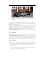
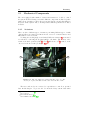
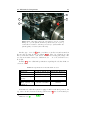
During autumn 2000 a final year project for the Master Students in Mechanical Engineering at Luleå university of technology, called “Sirius — Kreativ produktutveckling”, was initiated. On commission of Volvo Cars in Göteborg, the
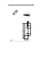
students implemented an X-by-Wire system into a car, a Tiger Cat E1 (see Figure1.1), using a new method specially designed to consider reliability during the
development process of coupled systems2 . The project ended late May 2001 and
the result was a four wheel steered car where all mechanical connections between
driver and the rest of the system were replaced with sensors, actuators and a distributed real-time controller network — see the Luleå Sirius project report [36].
Even though the car at this point was steerable, far from all the functionality the
equipment allowed was implemented in software.
1 The
2A
“X” in X-by-Wire could be replaced by “Brake”, “Steer” or “‘Clutch”.
collection of sub-systems, which depend on each other in order to function.
1
2
Introduction
Figure 1.1. The Tiger Cat E1 X-by-Wire prototype car (figure taken
from [36]).
The car was soon after moved to Volvo Cars in Göteborg where a couple of additional projects were performed before it arrived to the Department of Mechanical
Engineering, Linköpings universitet.
At this point the car was no longer functioning — the rear wheels had been
disconnected due do a replacement of sensors which had not been tested, and the
front wheels had almost a life of their own when driving the car. Also, the software
implementation of algorithms and regulators needed a fair amount of work.
This Master Thesis project was initiated in order to fix these problems, and
get the car up an running.
1.2
Purpose
The purpose of this report is not only to describe the work done during this project
— it should also serve as a shorthand introduction to the car, in order to lower
the threshold for future projects.
As the substance of the report is of a technical character, the intended reader
is a person with an engineering background. On the other hand, anyone with an
interest in the possible future of the vehicle industry would also benefit from it.
1.2.1
Objective
The main objective of this project is to modify the car so a useable and functional
concept prototype is obtained. To achieve this, the following goals have been set;
• The different parts included in the control system should be identified and
well documented.
• The implemented controllers and algorithms should be modified so the car
behaves in a consistent manner when driven.
1.3 Report Structure
3
• The system should be able to handle redundant components in order to
detect faults.
These goals should be implemented in hardware and software in such a way
that the car can be used as a platform for laboratory or research projects in the
future.
1.2.2
Limitations
As the objective definition is fairly open and the available time limited, a few
limitations on the scope of the project are applied .
First, no evaluation of the installed network or the protocol is performed. See
[14, 33] where the TTP/C3 and the CAN4 protocols are compared, and [22] for a
brief introduction to alternatives to TTP/C (TTCAN5 , FlexRay6 etc.).
As the first of the above goals states, only the parts which build up the X-byWire system are covered in detail. All other parts like the engine, power train,
ignition system etc. are only mentioned briefly.
The implementation of fault tolerance is also restricted to manage only fault
detection — not handle any failure modes. This means that the system should
be able to detect if, for example, a sensor is malfunctioning but not react in any
special way if, or when, that happens.
1.3
Report Structure
The report is structured as a working procedure for the system at hand. The
chapters describe the different steps involved when working with the system, and
their order resembles to the order in which the steps should be performed — i.e
before a controller structure can be made, demands on system performance are
needed, and a schedule cannot be made unless the all task are defined, which in
turn require detailed knowledge about the system. This is important to keep in
mind, specially for anyone who intends working with the system.
Chapter 2 gives an brief introduction to the car and its history. However, the
focus is on the installed parts and their function in the car.
Chapter 3 treats mechanical and electrical modifications that have been performed during the project.
Chapter 4 considers how to make all parts work together as a whole. This involve
a discussion on possibilities and drawbacks with a safety critical systems, as
well as considerations regarding algorithms and controllers.
3 Time
Triggered Protocol class C
Area Network
5 Time Triggered CAN
6 The FlexRay protocol was developed by the FlexRay Group which started as a co-operation
between BMW and DaimlerChrysler in 1998.
4 Controller
4
Introduction
Chapter 5 treats the actual construction and implementation of the algorithms
and controllers used. It describes the step from the overall demands to
something that can be used in practice.
Chapter 6 covers the steps to be taken to get the system up and running. This
involves defining tasks, messages, and a schedule7 .
Chapter 7 includes results from different tests performed on the system. It gives
feedback on how well the practical results relate to the simulated ones.
Chapter 8 summarizes the work done and presents conclusions made. Also, comments on future work are found here.
Appendix A gives an introduction to the software tools used to program the
network.
Appendix B presents a detailed diagram of the power distribution to the installed hardware.
Appendix C includes circuit diagrams for all adapting electronics used in the
car.
Appendix D gives an detailed explanation on how to connect the wires to the
circuit boards used.
Appendix E lists the manufacture drawings made.
7 This
is a description of when the system should do what.
Chapter 2
Inventory
Before any work can be done, detailed knowledge about the car and installed
components is needed. In this chapter, the car is first examined at a macro level to
give an overall picture. Later, each component in the X-by-Wire system is covered
in more detail, starting with the most complex part — the network. Thereafter
mechanical components such as sensors and actuators are analyzed, and last but
not least the surrounding electronics needed to adapt signals between components
and the network are examined. Please note, that the hardware listing only apply
to the car’s present state during the end of this project.
First, however, a clarification regarding the use of expressions should be noted.
In the following sections (and in the rest of the report) the expression “Node”
will be used frequently (Node CL for example). It should NOT be confused with
“PowerNode”, as “Node” refers to a collection of equipment fitted inside a protective housing, or the housing itself. The expression “PowerNode” refers to a special
piece of hardware and is part of the equipment inside the housing.
2.1
Car Overview
As mentioned briefly in Chapter 1, the car is a Tiger Cat E1 - a replica of the old
Lotus Super 7 racing car, but modified during a final year project by students at
Luleå university of technology into a complete X-by-Wire vehicle. In co-operation
with Volvo Cars in Göteborg the project design task was to deploy solutions for the
steering- and braking systems, in order to allow the car to turn around its own axle,
be moved in parallel, and have both the left- and right hand steering. Another
design task was to modify the engine suspension in order to reduce vibrations
during idle running.
At the end of the project the students had indeed succeeded in their task
and were able to demonstrate a functional prototype. To achieve their goals,
all mechanical connections between the driver controls (i.e. steering wheel and
pedals) and the rest of the car, were removed. Instead, sensors and actuators were
installed and connected via a distributed real-time controller network.
5
6
Inventory
To be able to switch between right and left hand steering, the students constructed movable modules of the steering wheel and the pedals, which easily could
be fitted to the left or right hand side. The modules are seen lying on the ground
in front of the car in Figure 1.1. As the car should be equipped with four wheel
steering, the rear suspension was completely modified and parts in the drive chain
had to be replaced with a type that would allow the wheel to change the steering
angle.
Also, the engine suspension was modified and an actuator was fitted on one of
the engine bearers. The actuator created vibrations in opposition on the engine’s,
and in that reducing the overall vibrations in the car. Although the actuator still
is fitted, it was just tested to verify its function and has never been used since.
Before going on specifying the components which constitutes the X-by-Wire
system, there are some parts worth mentioning which have not been modified
compared to the original car. Originally, the Tiger Cat E1 is composed of parts
from other car models, normally a Ford Sierra. This car is no exception. Under the
glass fibre cap, a 2.0 litre, 4 cylinder Ford engine is found, giving about 140 hp1 (in
this light car that gives enough power to do 0 - 100 km/h in less then 5 seconds).
Among other parts the Sierra has contributed with, are the two DELLORTO
DHLA 40 H carburettors, the 5-speed gearbox, and the ignition system.
2.2
Network and Connections
The real-time controller network plays a central role in an X-by-Wire system and
it has essentially three important tasks to perform;
Information exchange. When turning the steering wheel you would also expect
the wheels to turn. The network has to provide the connection between these
parts so they can communicate with each other.
Sensor data collection. When pressing the brake pedal, a sensor registers a
change in the pedal angle. The network then has to collect the sensor data
and translate it into a reference value for the brake pressure, for example.
Actuator control. Assume that a throttle valve reference value has been set,
and it has been correctly transmitted to the part where the throttle valve
actuator is connected. The network then has to make sure that the actuator
is in fact following that reference.
Some of the examples described above are critical for the function of the car,
and it is of great importance that the controller network can perform the tasks
with a high degree of safety and reliability.
For a long time now the car industry has been (and still is) using the CAN
protocol to communicate between different systems in a car, and is is sufficient for
the applications used today. However, it lacks many requirements, especially regarding safety, needed in a distributed safety-critical real-time system like this (i.e.
1 horse
power
2.2 Network and Connections
7
steer- and brake-by-wire applications). To meet these requirements the TTP/C
protocol was developed some ten years ago by the Vienna University of Technology and Daimler-Benz Research. Later, in 1998, an Austrian company, TTTech,
was formed to develop tools and hardware using the TTP concept. For a more
comprehensive introduction to the history of the TTP/C protocol, please refer to
[22].
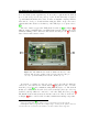
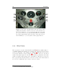
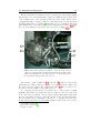
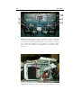
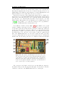
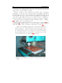
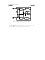
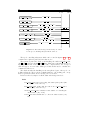
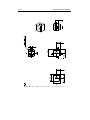
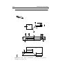
The base of this concept is the TTTech C1 PowerNode [41] (see Figure 2.1),
which is equipped with TTTech’s own TTP/C-C1 network controller chip for information exchange, and a Motorola embedded Power PC processor2 for sensor
data collection and actuator control.
1
2
Figure 2.1. The TTTech C1 PowerNode which form the base of the
network. The two large circuits on the board are the Power PC processor (no. 1) and the TTP/C-C1 network controller (no. 2).
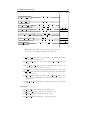
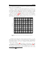
A network, or a cluster, is composed of two or more PowerNodes, which are
connected to each other via a broadcast data bus3 using either a “bus” or a “star”
network topology [42], and communicate using the TTP/C protocol. The network
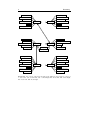
in this car consists of six PowerNodes located at strategic places (see below for
detailed locations), which are connected to each other using the bus topology 4 .
The installed sensors and actuators are in turn connected to these PowerNodes —
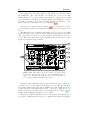
see Figure 2.2 where each PowerNode is listed with its surrounding components.
2 (MPC555
Black Oak, [30])
nodes participating in the cluster receives every message sent on the network.
4 Although the star topology introduces a higher degree of safety in the system, it has not
been used since the old version of the software tools used at Luleå did not support it.
3 All
8
Inventory
Brake limit switch
Brake limit switch
Brake pressure sensor
Brake pressure sensor
Brake actuator
Wheel angle actuator
Brake actuator
Node FL
Node FR
Encoder
Encoder
Linear potentiometer
Linear potentiometer
Carburettor choke
Throttle servo
Steering wheel MR-brake
Clutch actuator
Brake pedal MR-brake
Wheel angle actuator
Node CL
Node CR
Park brake switch
Indicators
Switches
Clutch pedal
Brake pedal
Throttle pedal
Steering wheel
Parking brake lock
Parking brake lock
Brake limit switch
Brake limit switch
Brake pressure sensor
Brake pressure sensor
Brake actuator
Wheel angle actuator
Encoder
Linear potentiometer
Speed sensor
Brake actuator
Node RL
Node RR
Wheel angle actuator
Encoder
Linear potentiometer
Speed sensor
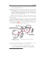
Figure 2.2. An overview of the network and how the different components are connected
to each other. CL - Central Left, CR - Central Right, FL - Front Left, FR - Front Right
RL - Rear Left, RR - Rear Right.
2.2 Network and Connections
2.2.1
9
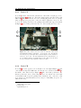
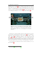
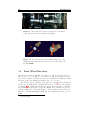
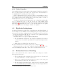
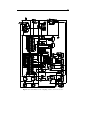
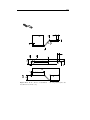
Node CL
Node CL5 is found on the left side, just in front of the dash board (the grey box to
the left in Figure 2.3), where it controls the clutch actuator and the brake pedal
MR-brake6 . The MR-brake is, however, not actually plugged into the node, but the
wires are prepared for prospective connection. Other equipment connected to the
node are the clutch pedal sensor, the parking brake switch (the upper left switch
in Figure 2.4), one brake pedal sensor and one of the steering wheel encoders.
1
3
2
4
Figure 2.3. The centre nodes are located on each side of the black
fuel tank in the middle of the figure — Node CL (no. 2) to the left and
Node CR (no. 4) to the right. Also seen in the figure are the carburettor
choke (no. 1) (i.e. the cold start enrichment device) and the fuse box
(no. 3), which contain power supply fuses for the centre nodes, the front
nodes, as well as for the actuators connected to these.
2.2.2
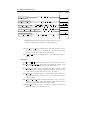
Node CR
Node CR7 is located opposite to Node CL (the box to the right in Figure 2.3) and
controls the steering wheel MR-brake, the throttle servo and the four LED:s8 in
the middle of the dash board (see Figure 2.4). The other brake pedal sensor, the
throttle pedal sensor, the second steering wheel encoder, and the rest of the dash
board switches (all except the parking brake switch) are also connected to this
node. Please note that all switches are two-way (i.e. ON/OFF), except for one,
which is three-way.
5 Central
Left
6 Magneto-Rheological
7 Central
Right
8 Light Emitting Diode
brake
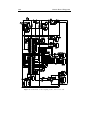
10
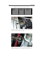
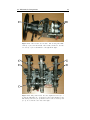
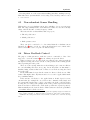
Inventory
1
4
2
5
3
6
Figure 2.4. The dash board with switches. The upper left one is the
parking brake switch (no. 2) and is connected to Node CL. The rest of
the two-way switches (no. 3, 6), as well as the single three-way switch
(no. 5), are connected to Node CR, and their function is controlled by
the software implementation in the PowerNode. The same is true for
the four LED:s (no. 1, 4), located just below the gauge indicators.
2.2.3
Wheel Nodes
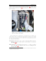
The four wheel nodes (Node RL, RR, FL, and FR9 ) all have similar tasks, i.e.
controlling braking and steering for one wheel each. The two front nodes are
located on either side of the radiator (see Figure 2.5) and the rear nodes are
located just behind the seats (see Figure 2.6). They are connected to the wheel
actuators, the wheel angle encoders, the wheel actuator potentiometer, the brake
actuators, and the brake pressure sensor. In addition to this, the two rear nodes
have a special brake directly attached on the motor axle on the brake actuators
(see below for details) and a speed sensor connected to them.
9 Rear
Left, Rear Right, Front Left and Front Right
2.2 Network and Connections
11
4
1
5
2
6
3
7
Figure 2.5. Node FL (no. 7) and Node FR (no. 3) are located on each
side of the core fan, and the motor control boxes for the front wheel
actuators are placed just in front of it. The two upper boxes (no. 1, 5)
control the brake actuators and the two lower ones (no. 2, 6) the steer
actuators. Also, in the top of the figure, the steer actuator choke box
(no. 4) is seen.
1
4
2
5
3
6
Figure 2.6. The rear nodes are placed just behind the seats – Node
RL (no. 5) behind left seat and Node RR (no. 2) behind the right. The
rear brake actuators are also located here, outside each node (no. 1, 4).
The two small holes in the middle are the battery master switches for
the 12 V (no. 3) and 24 V (no. 6) systems respectively.
12
Inventory
2.3
Mechanical Components
The car is equipped with a number of sensors and actuators to be able to control
the system. In the following sections the different components are listed together
with a short description of where they are mounted in the car and what function
they have in the system. Also, some important technical specifications are listed
in tables.
2.3.1
Actuators
There are three different types of actuators performing different types of tasks
- linear ball screw actuators for linear motion, servos for rotational motion and
MR-brakes for force feedback.
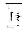
To change the steering angle, four identical ball screw actuators10 are mounted
at each wheel, connecting the steering spindle to the frame. The motions of the
actuators are made possible by DC11 motors12 with an encoder13 mounted on the
outer end of the motor axle (see Figure 2.7).
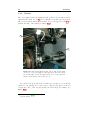
1
2
Figure 2.7. The rear right steer actuator DC motor (no. 1). The
encoder (no. 2) is seen mounted on the outer end of the motor axle.
The motor and encoder are connected to a special motor control box, specified
later in this chapter. To protect the box from the heavy current draw when
10 SKF
CARN 32x200x4, [38]
Current
12 maxon RE 40 148867, [25]
13 maxon HEDL-5540 110513, [29]
11 Direct
2.3 Mechanical Components
13
starting the motor, a choke14 have been inserted between the power cables (a
choke consist of two iron-cored coils connected in parallel, and are used to increase
a DC motor’s terminal inductance). The chokes are fitted in the car between the
rear motor control boxes (as shown in Figure 2.8) and on top of the front control
box mounting (the small gray box seen to the upper right in Figure 2.5).
1
2
Figure 2.8. The rear chokes inside its protective housing. The left
choke (no. 1) is connected to the left steer actuator DC motor, and the
right (no. 2) to the right motor. The chokes prevent the DC motors
from damaging the control boxes, by increasing the motors terminal
inductance.
As this car is a complete X-by-Wire vehicle, the clutch wire has been disconnected from the pedals and instead a ball screw actuator15 has been installed to
pull the wire. It is mounted just above the gearbox behind the engine — in the
centre of Figure 2.9 the circular shaped DC motor of the actuator is shown and
Figure 2.10 shows the actuator mounting above the gearbox. This actuator has a
sensor fitted inside, which measures the actuator length by detecting the position
directly on the moving nut. The DC motor is mounted on top of the actuator,
and together with the sensor it is connected to the clutch actuator control box.
Some specifications regarding the ball screw actuators mentioned above are
listed in Table 2.1.
14 maxon
15 SKF
133350, [28]
CAPR 43Ax100x2A1G3F / D24C, [37]
14
Inventory
Table 2.1. Specifications for the ball screw actuators.
Property
Function
Stroke
Gear ratio
Output speed range
Motor
CARN 32
Steering
200 mm
1:6.25
0 - 75 mm/s
maxon RE 40
CAPR 43A
Clutch
100 mm
1:12.5
0 - 26 mm/s
SKF D24C flat motor
Figure 2.9. The clutch actuator seen from above. The circular shaped
DC motor is seen in the middle of the figure.
Figure 2.10. The clutch actuator viewed from underneath the car.
Behind the aluminium gearbox, the mounting of the actuator is seen.
2.3 Mechanical Components
15
Except for the DC motors mentioned above, another type is used in the braking
system. Here, the conventional master cylinder (normally mounted just in front
of the braking pedal, on the separation wall between the engine and the driver
compartments) has been replaced. Instead, a system made up of four independent
hydraulic pumps has been designed [35], and fitted close to each wheel. The front
wheel pumps have been mounted inside each steering spindle (see Figure 2.11) and
the rear ones behind the seats, next to the rear nodes (see Figure 2.3).
1
2
3
4
Figure 2.11. The front left steer spindle - notice the brake actuator
pump (no. 3) in the middle of the figure, fitted inside the spindle. Other
parts seen in the figure are the brake caliper (no. 1), the armoured hose
(no. 2) and the brake pressure sensor (no. 4).
The actuator consist of a DC motor16 and a gearbox17 mounted on a steel block,
functioning as a cylinder. The motor operates on a piston inside the cylinder, via
the gearbox and a gear wheel. The original brake caliper18 has been connected to
the other end of the cylinder, via an armored hose.
To compensate for the increased oil volume, due to brake pad ware, a small
hydraulic tank with a non return valve have been fitted on the side of the steel
block. The valve prevents the oil from going backwards through the tank when
the piston is pushed forward, i.e. when the pressure in the system is increasing.
Two sensors have also been installed on the block — a pressure sensor has been
mounted just beside the hose, and a limit switch is found at the other end the
16 maxon
RE 35 118777, [24]
GP 32A 110367, [23]
18 Swedish: bromsok
17 maxon
16
Inventory
block. In Figure 2.12 all the different parts of the brake actuator have been laid
out - note the limit switch cables running out of the cylinder block.
In addition to the parts mentioned above, the rear DC motors have a special
brake19 directly attached on the motor axle. These brakes function as a park
brake by locking the axle when the power is turned off. Of course, the pressure
must first be increased in the system before the axle is locked, but that is handled
by the control system. The motor power cables are in turn connected to a motor
control box (specified later in this chapter), similar to the ones used for the wheel
actuator motors.
1
8
2
7
3
9
4
10
5
11
6
12
Figure 2.12. The different parts of the (rear left) brake actuator
pump. Starting from the left, the protective housing (no. 3) for the
DC motor and the gear box is seen, followed by the parking brake lock
mechanism (no. 1). Thereafter comes the DC motor (no. 2) and gear
box (no. 4) with the gear wheel (no. 5) just below. Then there is the
cylinder block (no. 10) with the limit switch (no. 7) in the top end
and the pressure sensor (no. 6) (together with a nipple (no. 12) for
connecting the hose) in the other. The last three parts are the piston
(no. 8), the hydraulic tank (no. 9) and the non return valve (no. 11).
In Table 2.2 specifications regarding DC motors and used gearboxes (when
appropriate) are found.
19 Östergrens
Elmotor AB FSB003, [32]
2.3 Mechanical Components
17
Table 2.2. Specifications regarding the DC motors and gear boxes.
Property
Function
Power rating
Nominal voltage
Gear box, ratio
No load speed
Max. continuous
current
Motor control
box
maxon RE 40
Steering
150 W
24 VDC
n/a
7580 rpm
maxon RE 35
Braking system
90 W
30 VDC
maxon GP 32A, 23:1
7220 rpm
SKF D24C
Clutch
n/a
24 VDC
n/a
n/a
6A
maxon ADS
50/10 201583
2.74 A
maxon ADS
50/5 145391
9A
SKF CAED
9-24R-PO
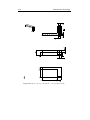
To be able to change the throttle valve opening in the carburettors, a servo 20
has been mounted underneath the intake manifold. Due to the lack of space, the
servo is not directly attached to the throttle valve — instead a flexible steel wire
has been installed between the servo output wheel and the valve arm (the wheel
is seen in Figure 2.13).
The carburettors also have a cold start enrichment device, commonly known
as a “carburettor choke” (not to be confused with DC motor chokes mentioned
earlier), which is controlled by a car door lock servo21 mounted behind Node CL
(see Figure 2.3).
20 HiTEC
21 VDO
HS-805BB+, [11, 12]
IMP 6880, no specification available
18
Inventory
2
1
3
Figure 2.13. The throttle servo (no. 2) viewed from above the carburettors. Just below the centre of the figure, the wheel (no. 3) attached
to the servo output is seen. Slightly to the left of that, connected to the
wheel, is the flexible steel wire (no. 1) going up to the throttle valve.
Last but not least, there are two MR-brakes installed in the car. They are both
used to apply some sense of force feedback to the driver by increasing the friction.
The first one22 has been attached directly on main shaft in the movable steering
module (see Figure 2.14). The second one23 has been installed in the pedal module
(see Figure 2.15) acting on the brake pedal.
The MR-brake in the steering module is controlled by a special control card24
located inside Node CR (the card is seen in Figure 2.21). The other MR-brake,
however, also needs a controller card similar to the other, but although preparations have been made to add one, the actual card is yet to be found.
22 LORD
RD-2028-18X-ol, [19]
MRB-2107-3, [18, 20]
24 LORD RD-3002-03, [21]
23 LORD
2.3 Mechanical Components
1
19
2
Figure 2.14. The movable steer module. The steering wheel MRbrake (no. 1) is seen in the middle of the module, and the two absolute
encoders (no. 2) are found further to the right in the figure.
1
4
2
5
3
Figure 2.15. The pedal module. Note the duplicated sensors (no. 1,
4) and the MR-brake (no. 3) attached on the brake (middle) pedal.
The clutch pedal sensor (no. 2) and the sensor for the accelerator pedal
(no. 5), are seen at the outer ends of the figure.
20
Inventory
2.3.2
Sensors
The car is equipped with both digital and analog sensors. At each wheel, a 14 bit
digital absolute shaft encoder25 has been installed to measure the wheel angle.
The encoders at the front have been mounted on top of the upper lever arm26 and
measure the angle of the spindle (see Figure 2.16).
1
2
Figure 2.16. The front right wheel angle sensors. The absolute shaft
encoder (no. 1) is seen mounted on the upper lever arm, and towards
the bottom right corner in the figure, fitted on top of the ball screw
actuator, is the linear position sensor (no. 2).
In contrast to the front wheel, the rear wheel encoders have not been directly
attached to the spindles due to lack of space. Instead, they have been moved
towards the centre of the car and measure the wheel angle via a linkage (see
Figure 2.17).
25 Hengstler
26 Swedish:
RA58-S, [8, 9]
länkarm
2.3 Mechanical Components
21
3
1
4
2
Figure 2.17. The figure shows the rear right encoder (no. 1) with
linkage (no. 3) to the spindle, the linear position sensor (no. 2) on top
of the ball screw actuator, and the speed sensor (no. 4) fitted inside the
spindle (partly concealed by the brake disc).
Another type of encoder27 with a resolution of 10 bit, is found mounted in
the moveable steering module (see Figure 2.14). Here, two identical encoders
have been mounted next to each other to measure the steering wheel angle. The
encoders are in turn connected to different nodes — one to Node CL and one to
Node CR.
In Table 2.3 some additional specifications regarding the absolute shaft encoders are found.
Table 2.3. Specifications for absolute shaft encoders
Property
Measures
Resolution
Code switching frequency
Supply voltage
Max current consumption
Leine & Linde 670
Steering wheel angle
10 bit (1024 inc/rev)
max 50 kHz
Hengstler RA58-S
Wheel angle
14 bit (16384 inc/rev)
max 100 kHz
9 - 30 VDC
70 mA @ 24 VDC
5 VDC
600 mA
As mentioned earlier the system is equipped with several analog sensors. On
top of the four wheel actuators, linear position sensors28 have been mounted (see
27 Leine
& Linde 670 670066350, [17, 16]
610, [1]
28 BEIDuncan
22
Inventory
Figure 2.16 and 2.17). In principle, these sensors are doing the same job as the
digital encoders mounted on the steering spindle, i.e. they measure the wheel
angle.
In the movable pedal module, four identical analog angular sensors29 are fitted,
which measures the angular displacement of the shafts when any of the pedals are
pressed (see Figure 2.15). The accelerator pedal and the clutch pedal have one
sensor each, and the braking pedal is equipped with two sensors.
The four independent brake actuators are equipped with one pressure sensor30
and one micro switch31 each. Both are mounted on the cylinder block (the pressure
sensor is seen at the bottom in Figure 2.12). The pressure sensor is of course used
for measuring the oil pressure in the system and the micro switch is used to indicate
when the piston is in its rear end position.
Finally, the car is equipped with two inductive speed sensors32 mounted inside
the rear steering spindles (see Figure 2.17). These sensors are used to measure the
wheel angular velocity, i.e. the speed of the vehicle, since the normal speedometer
is a pure mechanical construction. The sensors register the change in the magnetic
field when a tooth gap in the gear wheel, fitted on the axle shaft, passes by.
2.4
Power and Electronics
Not only does all equipment need some kind of power source in order to function,
the PowerNodes also need a number of surrounding electronic components to help
them interact with the rest of the parts in the system. These components are
classified into two categories — motor control boxes which amplify control signals
to the actuator motors, and electronics to adapt and filter signals coming in to
and going out of the nodes.
2.4.1
Electric Power Supply
As in all systems which include any type of electrical devices, a power supply is
needed. This car has two separate supply systems — one 24 V system and one
12 V system. The 12 V system is used for all the standard equipment in the car,
among these are the ignition system, head lights etc. It will not be described in
further detail in this report, since it does not interact with the “by-Wire” part of
the car. The 24 V system, on the other hand, is indeed interesting, since it supplies
power to all the added X-by-Wire equipment, i.e. network, nodes, actuator control
boxes, and sensors.
The base of the 24 V system consists of two 12 V 100 Ah VARTA batteries
connected in series. These are located at the back of the car (see Figure 2.18), and
are charged with a 24 V 70 A Motorola generator mounted on the right side of the
engine. One should note that, although the 12 V system is separated from the 24
V system, it is still connected to one of the batteries, making the load on the two
29 BEIDuncan
MOD.9811, [2]
0 265 005303, [3]
31 Saia-Burgess V4NCSK2, [34]
32 VOLVO 6849311 0988 10.0711-1146.1, no specification available
30 Bosch
2.4 Power and Electronics
23
batteries differ and the charging difficult. Because of this the batteries should be
shifted from time to time.
To protect the equipment, fuses have been put in between each of the connected
component and the power supply, i.e. each node and actuator control box has its
own fuse. These fuses are found inside two fuse boxes, located on just behind the
engine (see Figure 2.3) and above the batteries (see Figure 2.18).
There are also two battery master switches, one for each system, located between Node RL and Node RR just behind the seats in the car (the 24 V master
switch is the one closest to the nodes in Figure 2.3).
In Appendix B a schematic overview over the power distribution can be found.
2.4.2
Motor Control
There are three different types of motor control boxes in the car – one type for the
steering actuators, one for the brake actuators, and one for the clutch actuator.
The boxes make it easy to control the motors and remove the need for analyzing
the specific properties of the motor since the boxes are specially constructed for
the motor they are connected to.
There are a total of four steering actuator motor control boxes33 where two
are mounted in front of the radiator (the two lower ones in Figure 2.5) and control
the front wheel actuators. The other two are mounted behind the batteries (the
two closest to the batteries in Figure 2.18) and, of course, control the rear wheel
actuators. As seen in Figure 2.5, as well as in Figure 2.18, there are another four
motor control boxes34 not accounted for yet. These control the brake actuator
motors.
All of these eight control boxes can be configured to operate in different modes,
which specifies how the box should interpret the input, or command, signal. The
steer actuator control boxes have been set to “encoder” mode (refer to [27] for
details on how to configure the control box), since that will make the control box
interpret the input signal as a speed reference. The box will then automatically
adjust the output power so the angular velocity of the motor matches the specified
input voltage.
The brake actuator control boxes have, on the other hand, been set to “current”
mode (refer to [26] for details). The control boxes will in this mode interpret the
input signal as a current reference, and adjust the output current so the torque on
the motor axle matches the input voltage.
The clutch actuator control box35 is fitted inside Node CL (the black box in
Figure 2.19) and differs from the other control boxes as it is pre-configured to
function together with the actuator as a position servo, i.e. the input voltage
corresponds to a length on the actuator.
33 maxon
ADS 50/10 201583, [27]
ADS 50/5 145391, [26]
35 SKF CAED 9-24R-PO, [39]
34 maxon
24
Inventory
3
1
4
2
5
,
Figure 2.18. The actuator control boxes for the rear wheel actuators
are located just behind the batteries. The two boxes (no. 1, 4) closest
to the batteries control the steering wheel actuators and the other two
(no. 2, 5) the brake actuators. Also seen at the top of the figure, is the
fuse box (no. 3), containing power supply fuses for the rear nodes and
actuators.
Figure 2.19. The clutch actuator control box located inside Node CL.
2.4 Power and Electronics
2.4.3
25
Signal Adapting Electronics
Although the PowerNode is very advanced, there are some limitations to what it
can do. The maximum voltage allowed on the input pins (both on the digital I/O
pins and the analog ports) are 5 V and the output PWM36 channels can provide
signals between 0 and 5 V [41]. To handle these limitations adapting electronics
have to be used between the PowerNode and its surrounding equipment. The
electronics contribute with essentially three functions;
• Supply the sensors with power.
• Adapt and filter sensor signals to the PowerNode’s I/O ports.
• Amplify and filter control signals coming out from the PowerNode.
As the connected equipment differs between the PowerNodes, three different
types of circuit boards are found in the car — one type for the wheel nodes and
one type each for Node CL and CR. Although there are some differences between
the four wheel nodes (Node FL and FR lack speed sensors, and the parking brake
lock is only implemented in Node RL and RR) they still have the same type of
circuit board.
All circuit boards are supplied by the 24 V system, and the PowerNodes are in
turn supplied by the cards. However, in the two centre nodes (Node CL and CR)
a 12 V power cord is added to supply the MR-brake controller cards, the steering
wheel encoders, and the carburettor choke servo.
Another common factor between the different boards is the analog filters used.
They all are first order low-pass filters37 with a cut-off frequency at 16 Hz.
Two different types of operational amplifiers are also used on the boards. Although they differ in the allowed temperature range and surrounding components,
their task (with one exception, see below) is the same — to amplify a signal by
a factor of about 2 . To supply power to these amplifiers all boards have a 12 V
voltage regulator38 and a DC/DC converter39 fitted.
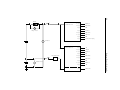
The circuit diagrams of the installed board types are found in Appendix C,
and in Appendix D a detailed description on how to connect the different wires to
the circuit board is found.
36 Pulse Width Modulate. A square wave signal where the average voltage is controlled by
changing the width of the pulse.
37 The filter is composed of one 2.2 µF capacitor and a 4.7 kΩ resistor.
38 The voltage regulator stabilizes an input between 15 to 35 V into a constant output of 12 V.
39 One input signal of + 12 V is converted into two output signals, one +12 V and one -12 V.
26
Inventory
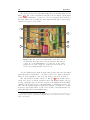
The circuit board for Node CL is fitted inside the node housing and is seen in
Figure 2.20. The connected digital steering wheel encoder has an output signal
voltage of 10 V, which has to be reduced to 5 V before going into the PowerNode’s
I/O pins. This is done by letting the 10 bit signal pass through a resistor bridge
and an electronic protection circuit.
1
4
2
5
3
6
Figure 2.20. The circuit board with adaptive electronics for Node
CL. Starting from the upper left corner, the following components are
pointed out; operational amplifiers (no. 1), relays (no. 2), 12 V voltage
regulator (no. 3), resistor bridge (no. 4) and protection circuit (no. 5)
for the encoder signal, DC/DC converter (no. 6).
To reduce high frequency ripple from the analog brake pedal sensor the signal
passes through a low-pass filter — the same is true for the clutch pedal sensor.
These two sensor signals are connected to the analog ports on the PowerNode.
The only actuators actually connected to this node40 is the clutch actuator,
via its own control box, and the carburettor choke. The required input to the box
is a smooth signal between 0 and 10 V, but due to the limitations in the PWMchannels on the PowerNode, the control signal has to be amplified by a factor of 2.
Also, since the PWM output is a square wave signal (i.e. contains a lot of high
frequency components), it has to be smoothed out. The control signal is therefore
passed through a filter and an amplifier stage.
40 As mentioned earlier, the brake pedal MR-brake is not connected due to the absence of a
controller card. However, a filter and an amplifier stage can be found on the card to adapt a
future control signal.
2.4 Power and Electronics
27
The carburettor choke servo is controlled by two relays — one for each direction.
The relays are supplied by the 12 V power cord and are directly connected to one
PWM-channel each. When the relay is switched on by the PWM signal, the 12 V
input is transferred to the output, where the servo is connected.
Last but not least, there is the parking brake switch. Here, no adaptive electronics is needed, i.e. the switch signal is directly passed through to the PowerNode
without any components in between. Do note though, that the switch signal is
not connected to one of the I/O pins (as would be expected), but to one of the
PWM-channels. Although the reason for this has not been explained (please refer
to [36, 35]), it is possible to do so, since the PowerNode can be programmed to
re-configure a PWM-channel into an I/O pin if needed.
Node CR has a circuit board (see Figure 2.21) quite similar to the one just
described. Similar components are used to adapt the second encoder signal, the
second brake pedal sensor and the throttle pedal sensor. This is also partly true
for the rest of the switches connected to this node, i.e. the signals are passed
through with no adaptive components in between. The difference is in the way
the switches have been connected to the PowerNode. Instead of using the I/O
pins or the PWM-channels (as been done in Node CL), the analog ports have
been used. Again, this is not as expected, but possible, way for connecting the
switches, since also the analog ports can be re-configured to function as I/O pins.
1
6
2
7
3
4
5
,
Figure 2.21. The circuit board with adaptive electronics for Node CR.
Note the special control card for the steering wheel MR-brake actuator
to the right (no. 6). Other components shown are the operational amplifier (no. 1), the resistor bridge (no. 2) and protection circuit (no. 3)
for the encoder signal, the DC/DC converter (no. 4), and lastly the 12
V (no. 5) and 5 V (no. 7) voltage regulators.
The connection of the dash board diodes are not that different compared to
the switches. They are also directly passed through to the PowerNode, but three
of them are connected to the PWM-channels and one to an I/O pin.
28
Inventory
Two actuators are controlled by this node, the throttle servo and the steering
wheel MR-brake. The control signal to the throttle servo does not need any
adjustment, but a 5 V voltage regulator has been fitted to supply the servo with
power. As with Node CL, there are adapting circuits for the MR-brake controller
card, but in contrast to Node CL, a card has actually been installed — it is
mounted directly on the circuit board as seen in Figure 2.21.
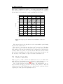
The wheel node circuit boards (see Figure 2.22) have been prepared for five
sensors and three actuators each, although some of them are not used in the front
nodes.
The simplest sensor to adapt is the wheel angle encoder, i.e. the encoder signal
is passed through to the PowerNode directly, without any circuits in between. The
only component needed is the 5 V voltage regulator, which supply power to the
encoder. The analog linear position sensor and the brake pressure sensor are also
supplied by the same voltage regulator.
2
3
4
1
5
6
,
Figure 2.22. The adaptive electronic circuit board for the wheel
nodes. The components are as follows; operational amplifiers (no. 1),
relay (no. 2), optically coupled logic gate (no. 3), 5 V (no. 4) and 12 V
(no. 5) voltage regulators, DC/DC converter (no. 6).
Both these analog signals are filtered, through the same type of filter used
everywhere else, to reduce high frequency ripple. Do note that after the filter,
the pressure signal is passed through an amplifier stage. The amplifier is needed
because only 20% of the signal range is used — the sensor output is 0 to 5 V
which corresponds to a pressure between 0 and 25 MPa, but according to [35] the
pressure in the braking system will not exceed 5 MPa.
As mentioned earlier in this chapter, the rear nodes have an additional speed
sensor fitted, which measures the speed by registering the change in a magnetic
2.4 Power and Electronics
29
field. The sensor output is a very week sinusoidal signal with a frequency proportional to the angular velocity of the wheel. Since the frequency is the desired
property to measure, a timer channel41 on the PowerNode should be used, and
the preferred input signal is a nice square wave shifting between 0 and 5 V. To
accomplish that, the sensor output is first amplified by a factor of 10 inside an
amplifier stage, and then passed through an optically coupled logic gate42 , which
creates a discrete signal with the same frequency as the input signal. In contrast
to all other circuits on the board, this logic gate is powered by the PowerNode.
The wheel and brake acutators connected to this node are controlled, via their
motor control boxes, by two PWM-channels each. This is due to the fact that the
control boxes have one input to run the DC motor in one direction and one for the
other. No different form the other cards, the control signals are passed through a
filter and an amplifier stage before leaving the circuit board. There is, however,
one exception — the signal to retract the brake actuator is not amplified [35].
Lastly, also just implemented in the rear nodes, a relay has been fitted to
control the park brake lock on the brake actuator motors (one for each actuator).
The relay is connected similar to the relays used in Node CL. The only difference
is the power supply — 24 V instead of 12 V.
41 An
I/O port which can, among other things, register the frequency of a signal.
trigger HCPL2200, [10]
42 Schitt
30
Inventory
Chapter 3
Modifications
Although much effort had been put down during the re-configuration of the car at
Luleå, some solutions have been found that need to be reviewed or modified. In
this chapter, some of the more important ones are discussed, which all have the
common aim to improve the overall system behaviour.
Both mechanical and electrical modifications have been performed on the car.
First a description of the problem and how it affects the system is presented. This
is followed by a presentation of the chosen solution.
3.1
Steer Actuator Joint
In the original version of the car, all of the wheel actuators were joined to the
spindles with a ball-and-socket joint, which allowed the outer part of the actuators
to twist. Since it is a ball screw actuator, the length is controlled by a motor acting
on a thread inside. Turning or twisting the inner part with respect to the outer
(without the motor running) will produce the same result as when one screws a
nut on a threaded bolt. This could be seen as disturbance or back-lash in the
control system.
The simplest solution for this is to replace the ball and socket mount with a
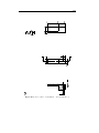
universal joint. In Figure 3.1 the old ball-and-socket joint (to the left) is seen
together with the new one (to the right).
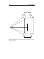
Since no commercially manufactured universal joints could be found that satisfied the requirements on dimensions, the joints were manufactured by the University workshop. In Figure 3.2 two views of the 3D model of the joint, made in
Pro/ENGINEER1, are seen. This model was the base, from which manufacturing
drawings were made (see Appendix E). Please note that no stress calculations
have been made on the joints. Normally, this should for course be included, especially for a safety critical part like this. However, after a discussion with the
experienced personal at the workshop, the conclusion was made that the material
choice and thickness should be sufficient for the time being.
1 A CAD (Computer Aided Design) software package provided by the company PTC
(http://www.ptc.com/ ).
31
32
Modifications
Figure 3.1. The modified steer actuator end joints - the old ball-andsocket joint (left) and the new universal joint (right).
Figure 3.2. An exploded (left) and assembled (right) view of the
manufactured universal joint. The 3D model of the joint was made in
Pro/ENGINEER.
3.2
Front Wheel Encoders
All wheel encoders had originally a resolution of only 10 bit, but it was soon
discovered not to be enough. So, new 14 bit encoders were purchased, but for
some reason, only the rear wheel encoders were actually fitted at that time. This
left the front encoders unchanged, which needed to be corrected.
Also, the encoders are mounted on the upper lever arm2 of the front wheels,
and the encoder shaft points downward and meets a rod welded to the spindles
(see Figure 3.3). When the suspension moves up and down, the rod and the
encoder shaft moves in respect to each other. Earlier, the rod and the encoder were
connected with a piece of gasoline tubing to allow for this movement. However,
this tube could flex significantly, which introduced disturbances in the encoder
signal.
2 Swedish:
länkarm
3.3 Wheel Actuator Control Boxes
33
One way to correct this problem is to move the encoder below the upper lever
arm and connect it to the spindle using some kind of linkage, similar to how the
rear wheel encoders are fitted (see Figure 2.17). Another way is to use some other
type of connection.
The first solution might be better because it can be difficult to find a connection
that has all the degrees of freedom, i.e. axial, radial, and angle displacement, to
the extent that is needed. On the other hand, it requires a quite large engagement
in the car to manufacture the linkage and the encoder mounting, and this was
beyond the scope of this project.
Figure 3.3. The front wheel encoders. The old 10 bit encoder with
the gasoline tube connected to the spindle is seen to the left, and to
the right is the new 14 bit encoder with bellow coupling.
Instead, the second solution was chosen and several different couplings have
been investigated. It were found that quite a few couplings allowed the required
degrees of freedom and among these were the curved-tooth gear coupling3 and the
bellow coupling4 , but none offered the extent of movement needed.
On the other hand, the springs in the wheel suspension have been tightened
to a maximum (probably done when this problem was first encountered). In
practice, this implies that the suspension will not move at all during normal driving
conditions, and therefore release the demands on coupling movement (this also
implies the car will not be very comfortable when driven).
The conclusion was to go for another coupling, despite that the requirement of
extensive movement was not fulfilled. Here, the curved-tooth gear coupling should
have been chosen, but instead a pair of bellow couplings were fitted, as they were
found among some spare parts to car.
3.3
Wheel Actuator Control Boxes
The housing for the wheel nodes were originally pretty crammed. Not only did
they house the PowerNodes and the adaptive electronic circuit boards, all the
3 Swedish:
4 Swedish:
bågtandskoppling
bälgkoppling
34
Modifications
actuator control boxes were also fitted inside (see Figure 3.4). As the control
boxes generate a fair amount of heat5 , and probably a lot of electrical noise, they
had to be moved.
Figure 3.4. The Node FR housing before the actuator control boxes
where moved in front of the radiator
The best solution in our opinion was to locate them as close as possible to the
actuator they control, i.e. brake and steering actuators. As there are not much
free space in the car where the boxes could be moved, the positions below were
the only practical alternatives;
Rear nodes A fair amount of space could be found just behind the batteries.
All four boxes could be mounted with a reasonable distance to the actuators
(see Figure 2.18).
Front nodes After some investigation it appeared to be enough room just in
front of the radiator fan, suitable for the four boxes controlling the front
wheels (see Figure 2.5).
5 Apparently the control boxes in the front nodes generated so much heat that the PowerNode
overheated and ceased to function.
3.4 Wheel Nodes Circuit Boards
35
With these locations some kind of additional housing to protect the control
boxes were needed, since the electrical connections otherwise would be unprotected. However, most of the other X-by-Wire equipment is at the present state
unprotected, so finding or designing a protective housing for the control boxes
alone, would not increase the system endurance by much.
Since suitable locations had been found, means of attachment had to be constructed. Using Pro/ENGEINEER, 3D models and manufacturing drawings (see
Appendix E) of appropriate attachments where produced and handed in to the
University workshop for fabrication. In Figure 3.5 and 3.6 the 3D models of the
attachments are seen.
Figure 3.5. Two views of the 3D model of the front wheel control
boxes, one explodes view (left) and one assembled (right).
Figure 3.6. The 3D model of the rear wheel control boxes, one explodes view (left) and one assembled (right).
3.4
Wheel Nodes Circuit Boards
The wheel node circuit boards had to be reviewed, due to a number of reasons.
First, as mentioned earlier in this chapter, the front wheel encoders had been
replaced by another type with higher resolution. Second, the speed sensors at the
rear wheel spindles had never actually been connected into the nodes and to do
that, new components where needed. Third, the old rear wheel node boards had
36
Modifications
a circuit fault — the PWM signal that supposed to retract the piston in the brake
actuator, was connected directly to ground.
Instead to continue to add and repair the old circuit boards, a new layout
was designed. To save time, the old layout was used as a template. Only small
modifications were done, in order to adapt the added equipment and take care of
the prior faults. The same board layout is used in all wheel nodes, although all
components are just utilized in the rear nodes. This was made to simplify for a
prospective addition of sensor in the front nodes, like speed sensors for example.
The circuit boards were manufactured in the University workshop — in Figure
3.7 the milling of the connection wires is seen.
For the complete circuit diagram of the board, please refer to Appendix C, and
in Appendix D a description on how to connect the actuator and sensor wires is
found. For a review of the board and its components, see Section 2.4.
Just before the printing of this report, a fault in the circuit board
design was discovered. The 2.2 kΩ resistor used for the pressure sensor
had been misplaced — instead of being connected in parallel between
the output signal and the 5 V power input, it was put in series with
the power input. However, it is possible to connect the sensor to the
board despite this error (see Appendix D for details).
Figure 3.7. The milling of wire connections on the wheel node circuit
boards.
Chapter 4
Synthesis
Until now, only the hardware installed in the car has been discussed, and nothing
has been said about how to make everything work together as a whole. The
glue to tie everything together is the algorithms used in the distributed realtime controller network. The network which not only renders the engineer almost
endless possibilities to control how the car should behave and feel when driven —
it also has drawbacks due to the increased complexity of the system that follows.
This chapter starts out by looking at some possibilities, as well as drawbacks
and safety issues, that an X-by-Wire system have compared to a “normal” mechanical system. In addition, demands on the systems involved are specified throughout
this chapter. These demands will be needed in Chapter 5.
4.1
Possibilities and Drawbacks
In an X-by-Wire system, the dynamics can be completely altered in software. All
that is needed, in principle, is to write an algorithm telling the system what it
should do, and when. In a car, this could be;
Using optimal wheel angles. Today, all cars have toe-angles1 built into the
wheel suspension to control the stability in acceleration or heavy break manoeuvres. In all other cases, toe-angles are just a drawback since they decrease the expected life time of the tires. To be able to dynamically control
when to use toe-angles, and when not to, could considerably reduce the
owners tire cost.
Parallel manoeuvres. Under certain conditions, a lane change on the freeway
or parking for instance, it could be desirable to move sidewise without having
the car turning.
Stability control during strong side wind. When driving a car in strong side
wind, the driver constantly has to compensate the wind forces that act on
1 A small angle on the wheel so that two wheels on an axle are not completely parallel to each
other.
37
38
Synthesis
the car in order to keep the car on the desired path. This could instead be
done automatically by the system.
Skid control. Some of the new cars today already have skid control systems (like
the DSTC2 system in Volvo XC90), but they all try to stabilize the car by
braking only. The performance could probably be improved by using both
steering and braking with an X-by-Wire system. The four wheel steering
also makes it possible to maintain control of the vehicle even if the front
wheels are locked in a panic brake situation.
All things presented in the list above cannot be realized in this car, in its
present state. However just small additions in hardware could make these things
(and more) possible.
The primary drawbacks in computer based controller systems regards reliability
and safety. These issues make it difficult to guarantee correct operation in all
situations. Pure mechanical systems have a big advantage in that respect —
faults are often both easier to spot at an earlier stage in the design process, and
fewer in quantity. Figure 4.1 points out some of the areas where safety issues have
to be considered, in addition to the pure mechanical ones.
Sensors
Computation and electronics
Communication
Actuators
Figure 4.1. Possible source of faults in the X-by-Wire system (drawing
made by Katja Tasala).
Numerous of incidents have happened over the years, which all are related to
hard or software faults in the computer based controller system:
In a computer controlled radiation treatment equipment (the Therac25), six accidents happened (where three people died of radiation
injuries) during the years 1985 - 87. The reasons were faults in the
2 Dynamic
Stability and Traction Control
4.2 Controller Structures
39
user interface, a 6 bit counter where set to 0, and a hardware lock
had been removed [40].
In 1992 a Boeing 767, belonging to Lauda-Air, suddenly changed the
jet drag direction during a fight [40].
Although it is not possible to guarantee a flawless system, the chance of stability
and correct functionality can be increased by using redundant3 components. Doing
that, though, presents new problems like choosing which component to trust in a
fault situation and which action to take if one or several of the components fail.
Again, it is the engineer who has to construct algorithms to handle that.
4.2
Controller Structures
The car presents opportunities and drawbacks not found in any of the commercially
available cars today. The wheel angles and brake pressures can be controlled
individually at each wheel, without the need of driver input. In fact, with some
small additions one could actually remove the driver entirely, and steer the car
remotely. The same contingencies4 also apply to the throttle valve opening and
the clutch. The only thing you still need to do manually in the car is shifting the
gears.
In order to control all these parts and make use of the performance built
into the car, controllers are needed. These controllers must be stable in every
situation, even if a sensor fails. To guarantee stability in a situation where a
sensor gives incorrect readings an open-loop controller is the safest alternative
since it stays unaffected. It can however be hard, or even impossible, to construct
such a controller if the system is non-linear or otherwise difficult to model.
4.2.1
Wheel Angle Controller
The wheel angle controllers job is to keep the wheel angles synchronized with a
commanded value, i.e. work as an angle servo. In addition it also have to keep
track of where the other wheels are when moving. A very important factor for the
cars stability is the aforementioned toe-angles. This makes it imperative for the
controller to, at all times, keep the wheels moving correctly with respect to each
other.
The main demand on a wheel angle controller is naturally stability. It has to
be, in every situation, stable since an oscillating wheel would surely result in a
violent crash.
In this particular application it is also important for the controller to be tolerant
towards model errors since the four wheels all have different parameters5 . The
parameters of a wheel can also change substantially when driving, if for instance
the road changes from tarmac to gravel.
3 Two
or more components doing the same job.
möjligheter
5 The electrical motors have different top speeds and the actuators have different friction.
4 Swedish:
40
Synthesis
4.2.2
Brake Controller
On a traditional car the pressure in the brake system is directly proportional to
the force that is applied to the brake pedal. It is the brake controllers mission to
accomplish this by controlling some sort of actuator.
When constructing the brake controllers, both speed and stability are important factors. The speed requirement is important since the latency between pedal
force application and pressure buildup must be as short as possible. As a rule of
thumb this latency can be no more than 100 ms.
To make the design stable in all situations the rule of thumb has, traditionally,
been to construct an open-loop controller. In the case of the braking system
implemented in the car, this is not possible since the brake actuator has very high
static friction6 . This makes an open-loop controller impossible since an applied
force on the piston is not directly proportional to the pressure.
4.3
Replicated subsystems
A replicated subsystem is defined as two identical systems with identical input. It
is, for example, used to minimize errors resulting from power outages which could
prevent a processor from completing its task. A redundant sensor is a special case
of a replicated subsystem, with only one component. The replicated subsystem
can contain any number of components.
In software there are a couple of replicated subsystems;
• The algorithm that calculates the wheel angles are implemented in software
on both center nodes and the algorithms are fed by the same input from the
network.
• Brake values are calculated in both center nodes.
For more information on the software, please refer to Chapters 5 and 6.
Hardware-wise there are also some replicated subsystem in the form of two
sensors measuring the same value. These can be found in the next section.
4.4
Redundant Sensor Handling
Some of the sensors in the car are doubled to make the readings more reliable.
The replicated sensors are;
• The steering wheel angle is measured by two independent encoders and each
encoder is connected to one of the center nodes.
• There are two identical sensors that measure the position of the brake pedal
and each sensor is connected to one center node.
• The wheel angles are measured in two ways; directly by an absolute digital
encoder and indirectly by measuring the length of the wheel angle ball screw.
6 The
force that must be overcome to start moving an object.
4.4 Redundant Sensor Handling
41
When using redundant sensors more difficulties arise. Merging sensor values
is a research area in itself which is called Sensor Fusion. Some of the problems in
this area are:
• How can the values be merged so that the result is in all cases better than
it should have been if using only one sensor.
• If the readings from a redundant sensor differ, which is correct?
More on this subject can be found in [7].
4.4.1
Wheel Angle Sensors
The two sensors that measure the wheel angle on one wheel do not have a linear
relationship to each other depending on the geometry of the suspension. This
means that the values have to be adapted to each other. One way to do that
is to look at the geometry of the wheel suspension and construct an algorithm
that takes either value and translates it to the other. This is however cumbersome
since it involves a whole lot of complex algebra due to the complicated geometry of
the suspension. A more practical solution is to create a lookup table to translate
between the values.
The dynamics of the steering, including actuator, motor and motor control box,
make it easy to model the behavior of the wheel. Since the input to the motor
control box is a reference value for the motor speed, a simple integrator with delays
taken from the data sheets of the motor control box and motor [25, 27] is a fairly
correct model (see Section 5.1 for a more detailed description of the model).
The model is used when comparing the two sensor values. In reality three
values for the wheel angle can easily be found; two measured and one calculated
using the output of the model when it is fed all earlier control signals. This makes
it possible to spot single errors7 by invalidating the sensor that deviates too much
from the calculated value. It is also possible to detect other errors; if for example
the two sensor readings are about the same, but differs a lot from the calculated
value, there is probably something wrong with the actuator or the motor.
The traditional way to achieve this kind of sensor fusion is to design a Kalman
filter. But since the wheel angle subsystem has almost no dynamics it is not needed
and this simpler approach can be used instead.
4.4.2
Steering Wheel and Brake Pedal Sensors
When measuring signals that are not controlled by the system, the task of sorting
out an erroneous sensor is more difficult. A predictor cannot be constructed and
only a few properties of the signals can be defined. For example; a sensor reading
that measures the steering wheel angle cannot change too quickly and it cannot
exceed some mechanical limits.
Using this a failing sensor can be detected if it changes rapidly but not if it has
a constant (or slowly changing) offset. In addition there is no way, in most cases,
7 When
one of the sensors fail.
42
Synthesis
of detecting which one of the sensors that is failing, just that something is wrong.
This makes these systems suitable for detecting errors, but they cannot be used
to correct errors.
4.5
Non-redundant Sensor Handling
Without the power of redundant sensors, the possibility to detect errors is pretty
slim. The only possibility left is to check if the sensor value exceeds some boundary
values, either in the time or in the frequency domain.
The sensors in the car that fall into this category are;
• Throttle pedal sensor
• Clutch pedal sensor
• Brake pressure sensor
These can all be considered to be less critical than the redundant sensors
discussed above8 , since even if one of these should fail and cease to function the
driver would still be able to stop the car without danger.
4.6
Driver Feedback Control
The purpose of this system is to make the car more comfortable to drive. It is
supposed to create the sensation9 that an ordinary car gives the driver.
When one drives a car, one can feel the forces that are put on the front wheels
through the steering wheel. One can also feel the pressure in the braking system
when depressing the brake pedal.
These are both very important factors when driving a car because it tells how
the car is handling and where it is going. In an X-by-Wire car this must be
simulated using actuators that brake or induce forces in the steering wheel and
the brake pedal.
In the Sirius 2001 Concept Car the means for driver feedback are two MRbrakes. This implies that only friction and no forces can be applied which make
the possibilities limited.
If the amount of feedback, i.e. the applied friction, should depend on some
external value (for example the error between the commanded wheel angle and
the current wheel angle) there could be cases where the brake could lock up the
steering wheel or brake pedal (example; if the brake pedal is depressed hard and
then released the feedback brake could lock the pedal in the depressed position).
This is naturally not the desired behavior. This restriction reduces the possibilities
of a realistic driver feedback even more.
8 Except for the brake pressure sensor, but the system was originally designed for traditional
open-loop brake controlling, i.e. this sensor was never planned to take part in a critical system.
9 Stiffness in the brake pedal and the forces from the road that can be felt in the steering
wheel.
4.7 Summary
43
All of those impairments really only leaves one realizable solution; the applied
brake friction should be proportional to the angular velocity of the steering wheel
respectively the speed which the brake pedal is depressed with. This is not really
a realistic feedback, but it is one solution which guarantees that the steering wheel
or brake pedal will not lock up in any position.
4.7
Summary
This chapter has outlined the most important properties that an X-by-Wire system
needs to have. Some of the advantages over conventional cars have also been
discussed.
Some demands on the controller structures have also been defined and these
will come to good use in Chapter 5.
44
Synthesis
Chapter 5
Implementation
In the previous chapter, the properties of an X-by-Wire system in general, and
the Sirius 2001 Concept Car in particular, were defined. In this chapter these
properties and demands are used to design controller structures for the individual
subsystems.
5.1
Wheel Angle Controller
The basic design goal behind this controller was to make as much use of the power
in the actuators as possible, while maintaining the stability of the system. Another
demand that needed to be fulfilled was that, when moving, the wheels must move
coordinated, even if they have different properties and commanded angles.
A “bang-bang” controller fulfills the basic demand, because it uses the largest
available control signal [6]. This makes the actuators move as fast as possible at
all times.
The bang-bang controller is, by design, very sensitive to noise in the measured
signals and can easily oscillate. To remedy this another controller is often used
for small errors. In this case a bang-bang controller was used for large errors and
a PI-controller, which was designed using Ziegler-Nichols [5], was used for small
errors.
1
controlled wheel
controlled wheel
2
other wheel
out
other wheel
bang-bang
|u|
1
out
0
In
Out
PI reg
Figure 5.1. Simulink model of the wheel angle controller.
45
46
Implementation
The wheel angle controller can be found in Figure 5.1. Note that the PIcontroller is fed a zero input until it is switched in to prevent the integrator from
winding up. The “other” input to the bang-bang controller is the error from the
other wheels. This will be further discussed below.
To construct the two controllers a model of a wheel is needed.
5.1.1
Wheel Angle Subsystem Model
The system that needs to be controlled when changing the wheel angle consists of;
• Motor control box
• Electrical motor
• Ball screw actuator
• The linear sensor that measures the length of the ball screw
• Wheel angle encoder
• Software in the PowerNodes
• The network
The software in the PowerNodes generates PWM-signals that are fed to the
motor control boxes. This makes the motor turn with an angular velocity that is
directly proportional to the PWM-value since the control box and the motor are
themselves a closed loop system. This removes nearly all of the motor dynamics
and simplifies the model a lot. When the motor turns the length of the ball screw
is altered and this in turn makes the wheel twist.
A fairly correct model for all this is a simple integrator with some delays in it.
This is reasonably correct, since the system (from PWM-value to angle alteration)
has nearly no dynamics and the PWM-value should be proportional to the wheel
angle velocity.
The amount of delay can be found by looking through the data sheets for the
different components [1, 8, 25, 27, 30, 38, 41];
Motor control box In the data sheet the bandwidth is found to be 2.5 kHz ⇒
1
−4
= 0.4 ms.
2500 = 4 · 10
Motor The data sheet states that the time constant is 5 ms.
Balls crew actuator The balls crew is completely rigid so the time constant is
zero.
Linear sensor The resistance changes instantly when the length of the sensor
changes. The PowerNode then samples this value, which adds a delay. The
data sheet for the Motorola PowerPC processor states that sampling takes
at least 14 QCLK, and the QCLK is 2 MHz ⇒ 7 µs.
5.1 Wheel Angle Controller
47
Encoder The data sheet states that the codes coming from the encoder can
1
= 1 · 10−5 = 10 µs.
change with a frequency of 100 kHz ⇒ 100000
Software algorithms This will take no longer than 5 ms.
Network The delay of messages on the network depends on the TDMA round
(see Chapter 6) which was chosen to be 10 ms. This delay will only affect
the messages that need to be transferred over the network.
In conclusion, the system that needs to be controlled, from PWM-value to
wheel angle, has a delay of roughly;
4 · 10−4 + 5 · 10−3 + 7 · 10−6 + 10 · 10−6 + 5 · 10−3 < 20 ms
plus an additional 10 ms for values that has to travel the network.
So an integrator with a time delay of 20 ms would be a reasonably good approximation for this system. The delay was chosen high since the practical resolution
in the finished system is 10 ms since the controller is updated every second TDMA
round (refer to Chapter 6 for more information).
1
motor_speed
in
out
Variable
saturation
T
1
z-1
z
1
z
Discrete-Time
Integrator
Unit Delay
Unit Delay1
1
wheel_angle
Figure 5.2. A somewhat simplified model of a wheel angle system.
A Simulink model of this can be seen in Figure 5.2 where the block called
“variable saturation” is a block that restricts how fast the wheel can move to
model friction and other disturbances. A more complete view of two wheels can
be seen in Figure 5.5 where the delays of the network messages can be seen.
5.1.2
Wheel Angle Predictor
The simple model that was defined in the last section is used to verify the sensor
readings. If this model is fed the same signals as the actual wheel, it would generate
a good estimate of the wheel angle.
This predicted value is used to verify that the values read from the two wheel
angle sensors are correct. If the sensors deviate too much, they are invalidated.
5.1.3
The Bang-Bang Controller
The bang-bang controller type was chosen because it makes as much use of the
hardware as possible by always using the largest possible control signal.
To make the wheels move synchronized the control signal that the bang-bang
controller would generate was adjusted so that the wheels would reach their commanded angle at the same time. This was implemented by taking the wheel with
48
Implementation
the greatest difference between commanded and actual angle and calculating how
much time it would take for this difference to vanish if the wheel traveled with
its maximum speed. This time was then used to calculate the speed by which the
current wheel would have to move in order to reach its destination at the same
time.
Introduce the variables;
α, β, φ, θ
ωα , ωβ , ωφ , ωθ
: Wheel angle errors for the four wheels
: Angular velocities for the four wheels
Using this, the time that a wheel takes to reach its destination, i.e. when the
wheel angle error equals zero, can be calculated as;
τα =
β
φ
θ
α
, τβ =
, τφ =
, τθ =
ωα
ωβ
ωφ
ωθ
The goal is that these times should all be equal to the largest time;
τ=
β
φ
θ
α
=
=
=
= max{τα , τβ , τφ , τθ }
ωα
ωβ
ωφ
ωθ
This is accomplished at the wheel with the wheel angle error α like;
max{τα , τβ , τφ , τθ } = τα
max{τα , τβ , τφ , τθ } = τβ
max{τα , τβ , τφ , τθ } = τφ
max{τα , τβ , τφ , τθ } = τθ
⇒
⇒
⇒
⇒
ωα
ωα
ωα
ωα
= ωmax
=α
β · ωβ
= αφ · ωφ
= αθ · ωθ
And similarly for the other wheels.
Using this technique, all wheels will reach their destination at the same time,
even if they have to travel different lengths and have different properties. It does
however involve some calculations that can be eliminated.
Suppose that all four wheels have the same top speed. This implies that the
wheel which has the largest angle error also will need the largest time to reach
its destination which in turn means that instead of comparing the time it would
take for the wheels to reach their destination one could compare the angle errors
directly. For the wheel with wheel angle error α this means that;
max{α, β, φ, θ} = α ⇒ ωα = ωmax
max{α, β, φ, θ} = β ⇒ ωα = α
β · ωmax
max{α, β, φ, θ} = φ ⇒ ωα = αφ · ωmax
max{α, β, φ, θ} = θ ⇒ ωα = αθ · ωmax
This eliminates the need to calculate the wheel angle velocity. It will also
protect the system if a wheel is stuck, since the other three wheels will still move
(although somewhat slower).
The assumption that the wheels have the same top speed can be made because
if a wheel has significantly lower top speed for a short period of time, for example
5.1 Wheel Angle Controller
49
2
wmax
1
controlled wheel
|u|
2
other wheel
>
1
out
|u|
inv
Figure 5.3. Simulink model of the bang-bang controller.
due to a puddle of mud, it is taken care of by the high sample rate. If it has lower
top speed for a long period of time, it is probably something wrong with the wheel
and it is more important for the other wheels to reach their destination quickly.
A Simulink model for the bang-bang controller for two wheels can be found
in Figure 5.3. In the model the controlled wheel angle error is first compared
to the largest of the other wheel angle errors. This comparison decides how the
wheel angle actuator should move; if another wheel has the largest angle error the
speed is set according to the rules above, otherwise the speed is set to the largest
available control signal (ωmax ) multiplied with the sign of the angle error (to make
the wheel turn in the right direction). The model can easily be extended to handle
four wheels by replacing the “other wheel” signal with the largest angle error of
the other wheels.
5.1.4
The PI Controller
To remedy the bang-bang controllers poor stability it is deactivated for small wheel
angle errors, instead a PI-controller is used. Ziegler-Nichols method [5] was used
to tune the parameters for this controller.
When tuning a controller using Ziegler-Nichols the steps below generate the
initial values.
1. Create a closed loop system with only proprotional control.
2. Increase the proportional gain until the system starts oscillating with a constant amplitude.
3. Note the gain and period of oscillation.
When this was used on the wheel model presented above in Figure 5.2, the oscillations began with a period of T0 = 0.1 s when the gain was K0 = 62.
With these values the Ziegler-Nichols rules give the controller parameters listed
50
Implementation
below;
P
: K = K20 = 31
T0
PI
: K = 0.45 · K0 = 27.9, TI = 1.2
PID : K = 0.6 · K0 = 37.2, TI = T20 , TD =
T0
8
when using a controller on the form;
1
u(t) = K(e(t) +
TI
Zt1
e(τ ) dτ + TD
d
e(t))
dt
t0
where e(t) denotes the wheel angle error as a function of the time t.
1
In
20
Kp
T
z-1
Discrete-Time
Integrator
1
Out
12
1 / Ti
Figure 5.4. Simulink model of the PI controller.
From these values the PI controller was chosen and the amplification was lowered somewhat to enhance the stability1 . A Simulink model of the PI-controller
can be seen in Figure 5.4.
5.1.5
Result
A model of the final system for two wheels can be seen in Figure 5.5. Note that
the two wheels can be fed different commanded angle values (the two steps to the
left). The two delays shown represents the delay when sending messages across
the network.
The model was tested by choosing different commanded values for the two
wheels and setting the disturbances in the “variable saturation” block differently
for the two wheels. The tests showed promising results and the wheel angles
followed each other nicely even if the commanded values and/or disturbances where
very different.
In Figure 5.6 a test run was made where one wheel was fed the commanded
angle of 2 (solid line) while the other one was fed a commanded angle of 1 (dashed
line). The variable saturation block was fed a white noise signal for both wheels
in this run.
1 The controllers speed is lowered due to this, but since it is only used for small errors this
will not affect the overall performance much.
5.1 Wheel Angle Controller
51
controlled wheel
Step
other wheel
out
motor_speed
wheel_angle
wheel1
controller1
1
wheel_angles
z
To Workspace
1
z
controlled wheel
Step1
other wheel
controller2
out
motor_speed
wheel_angle
wheel2
Figure 5.5. Simulink model which represents two wheels.
In Figure 5.7 the same commanded values as before were used, but one of the
wheels was disturbed by a sinusoidal signal instead of white noise.
52
Implementation
2.5
Relative angle
2
1.5
1
0.5
0
1
1.2
1.4
1.6
1.8
2
Time (s)
2.2
2.4
2.6
2.8
3
Figure 5.6. First test run of the wheel angle controller.
2.5
Relative angle
2
1.5
1
0.5
0
1
1.2
1.4
1.6
1.8
2
Time (s)
2.2
2.4
2.6
2.8
Figure 5.7. Second test run of the wheel angle controller.
3
5.2 Steer Algorithms
5.2
53
Steer Algorithms
This section discusses the problem of translating a given steering wheel angle into
commanded wheel angles. The algorithm plays a significant role in how the car is
behaving, which make it important that this is a well designed algorithm.
Everything that is said below assume that the wheels all roll without slipping.
This is of course far from the truth, but the results are nevertheless useful.
5.2.1
Ackermann Steering
When a car performs a turn the inner and outer wheels roll on different radii. To
prevent the tires from skidding, the inner wheels must turn with a greater angle
than the outer wheels. This is called Ackermann steering and is often measured
in percentage of true (i.e. 100%) Ackermann. An explanatory sketch can be found
in Figure 5.8.
Using 100% Ackermann the four wheel angles can be calculated as;
tan α
=
tan β
=
tan γ
=
tan δ
=
l−c
r− 2b
l−c
r+ 2b
c
r− 2b
c
r+ 2b
when using the notation given in Figure 5.8.
Traditional cars never have true Ackermann because the wheel angles are always a compromise between stability and tire wear. In the car at hand, all wheel
angles can be set independently of the others, which make true Ackermann an
obvious choice.
5.2.2
Steer Angle Distribution
For a traditional two wheel steered car the center of rotation is always fixed to the
rear axle. This is not the case for a four wheel steered car, where the center of
rotation can be put anywhere on a line going through the middle of the car. It is
also possible to control how the car is orientated during the maneuver.
If the steering angles on the front and rear axle are equal, the car can move sideways without rotating. This can be good for lane changing or obstacle avoidance
since the car avoids rotating. The maneuver can be seen in Figure 5.9.
Another special case is when the center of rotation is set in the middle of the
car. This lets the car turn with the shortest radius, and this is especially good for
parking and maneuvering in tight places.
However, under normal driving conditions none of these two special cases are
usable since the car behaves very differently from a conventional car, and the
driver will have a difficult task just controlling the car. Instead some algorithm
that steers the rear wheels with less extreme angles is needed. In such an algorithm
the relationship between front and rear steer angles can be dependent on dynamic
parameters such as the forward speed or the yaw rate.
54
Implementation
b
+
+
l
β
α
+
γ
r
δ
c
+
+
Figure 5.8. Explanation of true Ackermann Steering. Note the difference between α
versus β and γ versus δ.
5.2 Steer Algorithms
55
Figure 5.9. How a four wheel steered vehicle makes a parallel maneuver.
Introduce the variables;
δf
δr
Cf
Cr
lf
lr
m
V
θ̇
:
:
:
:
:
:
:
:
:
Forward steer angle.
Rear steer angle.
Traction on the front wheels in [N/rad].
Traction on the rear wheels in [N/rad].
Distance between the mass center and the front axle.
Distance between the mass center and the rear axle.
Mass of the car.
Forward velocity.
Yaw rate.
Sridhar and Hatwal [15] discuss five different steering models during a lane
change maneuver;
A Rear steer angles are kept at zero resulting in a behavior like that of a two
wheel steered car.
B The relationship between forward and rear steer angles involving the forward
velocity with;
δr = K · δf with K =
Cf lf mV 2 − 2Cf Cr lr (lf + lr )
.
Cr lr mV 2 + 2Cf Cr lf (lf + lr )
If the front steer angles are specified this algorithm gives rear steer angles
that are well adapted to the car.
C A model where the rear steer angle depends on the front steer angle and the
yaw rate;
δr = K · δf + C1 · V · θ̇ with K = −1 and C1 =
lr
lf
m
(
+
).
2(lf + lr ) Cf
Cr
56
Implementation
In addition to algorithm B this one takes the cars yaw rate into account to
prevent the car from skidding.
D The rear steering depends on the product of the yaw rate and forward velocity;
δr = C2 V θ̇ with C2 =
lf
lr
m
(
−
).
2(lf + lr ) Cr
Cf
Like algorithm C the yaw rate is taken into account when calculating the
rear steer angles. This one has however a different, nonlinear, relationship
since it depends on the product between forward velocity and yaw rate.
E The front and rear angles are individually and optimally controlled (hypothetical model).
Note that algorithm A through C give negative2 values for the rear steer angles
when the forward speed is low, and algorithm D gives positive values for all speeds.
If the rear steer angles are negative, the center of rotation is placed inside the car.
This will lower the minimum turning radius, thus making the car more maneuverable. If the angles are positive then the center of rotation is placed outside of the
car, which will lower the yaw rate and therefore the risk of skidding.
Sridhar and Hatwal [15] come to the conclusion that model D has the best
characteristics from the point of view of steering effort. It is also the only of the
models that produces neutral steer characteristics. Models B and C both produce
extreme under steer. However the only realizable four wheel steering model of the
ones listed above would be B since the car has no yaw rate sensor.
The yaw rate could however be calculated by using the speed sensors, to measure the difference between the speed of the inner and outer wheels. This would
imply that all wheels must roll without slipping, that assumption can only be
made for small velocities [31] so the calculations will not produce a reliable value
on the cars yaw rate.
5.3
Brake Force Controller
The demands on the brake controller is mainly stability. The function of the brake
system must also stay unaffected even if a sensor should fail. Therefore it is often
common to use an open loop controller. However, the brake actuators in the car
have so high static friction that this is not possible. To design a usable system the
controller must be able to overcome this friction and at the same time guarantee
stability.
Apart from the static friction the system is very simple. The control signal is
sent as a PWM signal to the brake motor control box. The box is set for current
control so the PWM signal is proportional to the current and therefore the torque
on the motor axle. This torque is transferred to the piston via a gear box. When
the piston moves the pressure is built up in the braking system and the brake pads
are pressed against the brake disc.
2 If
the front wheels turn left, the rear will turn right.
5.4 Braking Algorithms
57
One possible solution to this problem that maintains the open loop structure
is to generate the control signal as a linear combination of the commanded force
and its derivate. So if r(t) is the commanded force and u(t) is the control signal
that is fed to the brake motor control box as a PWM signal, the expression would
look like this;
d
u(t) = A · r(t) + B · r(t).
dt
Where A and B are constants.
This design will have problems if the brake pedal is depressed or released slowly
(i.e. during normal driving conditions). So it is not really usable for this system.
The open loop design must be sacrificed in this case, and a controller using the
brake pressure as feedback is used. This is a bad choice since the brake pressure
sensor is non redundant, and since it is an analog sensor it is vulnerable to noise,
but unfortunately it is the only choice.
5.4
Braking Algorithms
The brake algorithm that is implemented in the car is a very simple one with
a static brake distribution that always maintains a fixed ratio between the front
and rear axle. The possibilities are however almost endless for more advanced
algorithms.
One example is to distribute the brake force differently on the outer and inner
wheels when cornering. The outer wheels have higher contact forces so they can be
braked harder than the inner wheels. A car that implements this and is available
today is the top of the line Mercedes-Benz SL 500 coupe/roadster which has a
system called Sensotronic Brake Control. This system is reviewed in more detail
in [13].
58
Implementation
Chapter 6
Schedule
This chapter outlines the steps involved in scheduling this particular real time
system. This involves defining subsystems, tasks and messages.
6.1
The Time-Triggered Architecture — the TTP/C
Protocol
Before describing the schedule, a short introduction to the TTP/C is appropriate.
For a more thorough explanation and the history of TTP/C [22] is recommended.
TTP/C is a communication system of class C, and must therefore be strongly
deterministic. This means that the behaviour of the system must be known beforehand, and some rules must be set up for it. These rules should include how
and when both communications and computations are made.
All the rules put together form the schedule.
6.2
Subsystems
A subsystem can be seen as a set of tasks, or functions, that all collaborate to
achieve a more complex function. In a TTP/C cluster, a subsystem can be completely replicated, partially replicated, or non-replicated. A replicated subsystem
is run by several nodes in the cluster, and this makes the system dependable even
if a node should fail.
In an X-by-Wire application it is logical to divide the system into steering and
speed controlling subsystems. In the car, all of the nodes must run both these
subsystems since they are all involved in controlling both steering and the speed.
In addition two other subsystems, supervision and calibration, have to be defined to make the car more dependable and easier to maintain and setup. These
subsystems are also run on all nodes, naturally since all nodes have sensors that
need calibration and it is important to supervise all nodes.
Finally a subsystem that is responsible for driver feedback is defined. This
subsystem is only run on the two center nodes.
59
60
Schedule
Table 6.1. The subsystems and their responsibilities.
Subsystem
Steering
Speed controlling
Supervision
Calibration
Driver feedback
Center nodes
Read steering wheel
Calculate wheel angles
Read brake pedal
Calculate brake values
Read clutch pedal (only CL)
Read throttle pedal (only CR)
Read switches
Control indicators
Create status
Calibrate
Calculate feedback
Actuate feedback
Wheel nodes
Read wheel angle
Turn wheel
Read brake pressure
Actuate brake
Read wheel velocity
Create status
Calibrate
Not implemented
A summary of all of the subsystems can be found in Table 6.1.
6.2.1
Steering
For the two center nodes, the steering subsystem includes reading the steering
wheel angle and calculating the four commanded wheel angles, one for each wheel.
This subsystem is completely replicated since the two centre nodes make exactly
the same calculations, so even if one of the nodes should fail the system will
still work. However, if both of the center nodes are functional, the values of the
commanded wheel angles from them will be exactly the same.
Each wheel node then recieves its commanded wheel angle and tries to control
the actuator so that the wheel achieves this angle. In addition every wheel node
has to check that all of the wheels are turning with respect to each other. The
wheel nodes also have the responsibility to read the two sensors that measure the
current wheel angle and report this to the rest of the system.
6.2.2
Speed Controlling
In this subsystem the two center nodes read out how the pedals are positioned.
These values are then used to control the clutch actuator (for the CL node), the
throttle servo (for the CR node) and to calculate brake values for the four wheels.
The brake values are calculated in both nodes, but clutch and throttle are only
considered in one node each. This design choice was made since if, for example, the
CL node should fail, there would be no way of controlling the clutch actuator or
read out the clutch pedal value, since these are only connected to this node. This
makes the speed controlling subsystem in the centre nodes partially replicated.
The wheel nodes use the brake value calculated by the centre nodes to control
the brake actuators. This subsystem also has to read out the speed and brake
6.3 Tasks and Messages
61
pressure of each wheel. Currently the speed can only be read from the two rear
wheels since there are no speed sensors on the front ones. In addition, the dash
board switches are monitored to decide if the parking brake should be applied.
6.2.3
Supervision
The supervision subsystem is responsible for generating a status message for a
node. The status is made up from the status of all the subsystems that the node
runs and provides a simple way to see if a subsystem has any kind of problem.
In addition this subsystem is responsible for reading the dashboard switches
and setting the indicators. This is only done in the center nodes.
6.2.4
Calibration
The wheel nodes need a translation table to be able to match the readings from
the wheel angle encoder and the linear sensor measuring the actuator length. It
also needs information of the mechanical limits for the wheel. In addition the
brake pressure sensor must be calibrated. All these tasks are performed by the
calibrating subsystem. The system receives information from the center nodes if
it should go into calibration mode and if it should perform any calibration action
(such as store left limit, create lookup table, etc.).
Both of the two center nodes read the dash switches to decide if it should
switch to calibration mode and generates a message to the wheel nodes. It also
has to store its own calibration settings for the steering wheel and the pedals.
6.2.5
Driver feedback
This subsystem, which is only run on the center nodes, controls the MR-brakes
that are connected to the steering wheel and the brake pedal. It is supposed to
make the driving experience more comfortable and somewhat similar to that of a
conventional car.
The possibilites are rather limited since only brakes, which only can produce
friction, and not motors, which also can produce torque, are fitted in the car. If
these brakes were to be replaced with motors, a lot more advanced feedback could
be implemented.
6.3
Tasks and Messages
The subsystems are further divided into distinct tasks which would be easy to
implement in software. Each task is then implemented as a single function when
programming. The tasks exchange data with each other via messages that can be
global or node local.
The tasks and messages are scheduled in a TDMA1 round. Tasks are run once
every second TDMA round and messages have a lifespan of two TDMA rounds.
The TDMA round was chosen to 10 ms.
1 Time
Division Multiple Access
62
Schedule
Local
read swheel
Global
Swheel Enc Raw
Swheel Angle
check swheel
calculate wheel angles
Swheel Angle, Swheel Enc Raw
Swheel Angle
Swheel Angle, Switches
Steer Value **
Figure 6.1. The tasks, messages and how they are related
for the steering subsystem in the CL node.
In the schedule, each task is allocated a time budget and a deadline. The time
budget states how much processor time the task is allowed. Tasks that involve
calculations are allowed 200 µs, and other tasks are allowed 100 µs. The deadline
specifies when (in the TDMA round) the task execution must be finished.
The time budgets are chosen to “be enough” — no WCET2 calculations have
been made since this is very hard to do analytically [4].
In all the graphs in this section the boxes to the left are the tasks, the horizontal
arrows are messages and the two vertical arrows to the right are the local and the
global message space. Messages that end in the local message space stay on the
node and those that end in the global space are broadcasted on the network.
Whenever a message is ended with “**” below it means that there are actually
several copies of this message. One for each wheelnode (replace the “**” with
FL, FR, RL or RR) and in some cases additional messages for the center nodes
(replace the “**” with CL, CR).
6.3.1
Center nodes
In figures 6.1 and 6.2 the steering subsystem for CL and CR respectively are found.
This subsystem is replicated so the graphs are identical.
They start out by reading the steering wheel encoder, and after that this value
is compared to the value that the nodes agreed on in the last round to verify that
the encoder is working. The agreed value is then broadcasted to the network.
This value combined with the state of the dashboard switches (to select different
steering modes) is then used to calculate the four commanded wheel angles.
Below is a more in depth description of the tasks and messages involved in the
steering subsystem on the center nodes.
2 Worst
Case Execution Time
6.3 Tasks and Messages
63
Local
read swheel
Global
Swheel Enc Raw
Swheel Angle
check swheel
calculate wheel angles
Swheel Angle, Swheel Enc Raw
Swheel Angle
Swheel Angle, Switches
Steer Value **
Figure 6.2. The tasks, messages and how they are related
for the steering subsystem in the CR node.
Tasks
read swheel Reads out a value from the ten bit steering wheel encoder.
check swheel Checks that the value read by read swheel is sane.
calculate wheel angles Produces the commanded wheel angles.
Messages
Swheel Enc Raw The raw value as read from the 10-bit encoder that is
attached to the steering wheel.
Swheel Angle An agreed value representing the steering wheel angle,
with negative values when the steering wheel is turned left and
positive when it is turned to the right. The message comes replicated from both center nodes.
Switches This message is used to select which algorithm the calculate wheel angles task should use.
Steer Value ** Commanded wheel angle for a wheel. A negative value
means that the wheel should be steered left and a positive that it
should be steered right.
64
Schedule
Local
read clutch pedal
Pedal Clutch Raw
read brake pedal
Pedal Brake Raw
check clutch pedal
Global
Pedal Clutch Raw, Pedal Clutch Value
Pedal Clutch Value
Pedal Brake Value
check brake pedal
calculate clutch value
calculate brake values
Pedal Brake Raw, Pedal Brake Value
Pedal Brake Value
Pedal Clutch Value
Clutch Value
Pedal Brake Value, Switches
Brake Value **, Park Brake **
Calibration Mode
actuate clutch
Clutch Value, Calibration Mode
Figure 6.3. The tasks, messages and how they are related
for the speed controlling subsystem in the CL node.
The speed controlling subsystem, which can be found in figures 6.3 and 6.4,
contains some replicated parts and some that are not.
The replicated part is the brake pedal handling; the tasks read brake pedal,
check brake pedal and calculate brake values. This part works just like the steering subsystem; it first reads a raw sensor value, compares this to the old agreed
value and agrees on a new value. This agreed value is then used to calculate the
commanded brake forces.
The clutch and throttle handling are the un-replicated part of the speed controlling subsystem. They work in a similar fashion to the braking part, except
that no agreement is made and no messages are broadcasted.
Below is a short description of all the tasks and messages involved:
Tasks
read clutch pedal Gets a raw reading of the clutch pedals position (this
is only done on the CL node).
check clutch pedal Verifies that the value from read clutch pedal is
correct (only on the CL node).
calculate clutch value Calculates a value suitable for controlling the
clutch actuator (only on CL).
actuate clutch Sets PWM value to control the clutch actuator (only
CL).
6.3 Tasks and Messages
65
Local
read throttle pedal
Pedal Throttle Raw
read brake pedal
Pedal Brake Raw
check throttle pedal
Global
Pedal Throttle Raw, Pedal Throttle Value
Pedal Throttle Value
Pedal Brake Value
check brake pedal
calculate throttle value
calculate brake values
Pedal Brake Raw, Pedal Brake Value
Pedal Brake Value
Pedal Throttle Value
Throttle Value
Pedal Brake Value, Switches
Brake Value **, Park Brake **
Calibration Mode
actuate thottle
Throttle Value, Calibration Mode
Figure 6.4. The tasks, messages and how they are related
for the speed controlling subsystem in the CR node.
read throttle pedal Gets a raw reading from the throttle pedal (this
is only done on the CR node).
check throttle pedal Sees if the value that read throttle pedal reads
is sane.
calculate throttle value Generates a value that can be used to control the throttle servo (only on CR node).
actuate throttle Generates PWM signal from throttle servo (only CR).
read brake pedal Reads a raw value from the brake pedal. This task is
run on both nodes.
check brake pedal Checks the values from read brake pedal to see if
they are correct. This task reads values from both nodes and compares them.
calculate brake values Calculates commanded brake forces for all four
wheels.
Messages
Pedal Clutch Raw Raw value from the clutch pedal.
Pedal Throttle Raw Raw value from the throttle pedal.
Pedal Brake Raw Raw value from the brake pedal.
Pedal Clutch Value Verified value on the clutch pedal.
66
Schedule
Local
read switches
actuate indicators
Global
Switches
Switches, Calibration Mode,
Node Status **
Swheel Angle
supervise cnode
calibrate cnode
calculate feedback
actuate feedback
Swheel Angle, Pedal Brake Value,
Pedal Clutch Value
Pedal Brake Value
Node Status C
Swheel Enc Raw, Pedal Clutch Raw,
Pedal Brake Raw, Switches
Switches
Calibration Mode
Swheel Angle, Pedal Brake Value
Swheel Feedback, Brake Feedback
Swheel Feedback, Brake Feedback
Figure 6.5. The task, messages and how they are related
for the supervising, calibrating and feedback subsystems in
the CL node.
Pedal Throttle Value Verified value on the clutch pedal.
Pedal Brake Value Agreed value from the brake pedal. This message is
produced in both center nodes.
Clutch Value Value that represents the commanded position on the
clutch actuator.
Throttle Value Value that is the commanded position on the throttle
servo.
Brake Value ** Commanded brake force for wheel FL, FR, RL and RR.
Park Brake ** This message contains a 1 if the park brake on wheel FL,
FR, RL or RR should be applied. Otherwise it is 0.
Calibration Mode This is used to prevent the different actuators from
moving when the system is in calibration mode.
The supervising, calibrating and feedback subsystems can all be found in figures
6.5 and 6.6.
Supervising is done by checking the status of all messages that are produced
by the node. The resulting message is calculated as the sum of the messages from
CL and CR. The supervising subsystem also reads out the dashboard switches and
controls the indicators to inform and warn the driver.
6.3 Tasks and Messages
67
Local
read switches
actuate indicators
Global
Switches
Switches, Calibration Mode,
Node Status **
Swheel Angle
supervise cnode
calibrate cnode
calculate feedback
actuate feedback
Swheel Angle, Pedal Brake Value,
Pedal Throttle Value
Pedal Brake Value
Node Status C
Swheel Enc Raw, Pedal Throttle Raw,
Pedal Brake Raw, Switches
Switches
Calibration Mode
Swheel Angle, Pedal Brake Value
Swheel Feedback, Brake Feedback
Swheel Feedback, Brake Feedback
Figure 6.6. The task, messages and how they are related
for the supervising, calibrating and feedback subsystems in
the CR node.
The tasks and messages in the supervising subsystem on the center nodes are:
Tasks
read switches Creates a message containing bits for all switches on the
dash board.
actuate indicators Controls the various indicators on the dash board.
supervise cnode Checks the total status of the node by analyzing the
messages that the other tasks on this node produces.
Messages
Switches State of the dashboard switches. Each bit in the message
represents one switch; if the switch is on the bit is 1 otherwise the
bit is 0.
Calibration Mode This message is used to inform the user if the system
is in calibration mode.
Node Status ** The system uses these to inform the driver of any faults
in the system.
Node Status C This message contains the status of the two center nodes.
It is created using the status information from the messages Swheel Angle,
Pedal Clutch Value, Pedal Throttle Value and Pedal Brake Value.
68
Schedule
Calibration mode is chosen with the dashboard switches, and the procedure is
then stepped through by operating another switch. Calibration is made by storing
raw sensor readings in the PowerNodes memory. The calibration task on the center
nodes must also create the calibration mode message to inform the other nodes.
Finally the driver feedback subsystem consists of two tasks and two messages;
Tasks
calculate feedback Calculates values for the feedback by looking on
the steering wheel angle and the brake pedal value.
actuate feedback Uses the value calculated by calculate feedback to
control the magneto reological brakes that are fitted to the steering
wheel and the brake pedal.
Messages
Swheel Feedback The amount of feedback that should be applied to the
steering wheel. It is created using the Swheel Angle message.
Brake Feedback Amount of feedback that should be applied to the brake
pedal, created using the Pedal Brake Value message.
6.3 Tasks and Messages
69
Local
read encoder
Global
Wheel Encoder Raw FL
read actuator len
Wheel Actuator Len Raw FL
Wheel Angle FL
check wheel angle
Wheel Angle FL, Wheel Actuator Speed FL,
Wheel Encoder Raw FL, Wheel Actuator Len Raw FL
calculate actuator speed
Wheel Angle FL
Wheel Angle **, Steer Value **
Wheel Actuator Speed FL
Calibration Mode
actuate wheel angle
Wheel Actuator Speed FL, Calibration Mode
Figure 6.7. The tasks, messages and how they are related
for the steering subsystem in the front left wheel node.
6.3.2
Wheel nodes
All of the four wheel nodes run the same tasks, but they produce different messages.
For example; the front right node produces a message called Wheel Angle FL while
the front right node produces Wheel Angle FR.
Figures 6.7, 6.8, 6.9 and 6.10 list the tasks and messages for the steering subsystem.
This subsystem starts out by reading the raw sensor values that measure the
wheel angle. These two values are also broadcasted for debugging purposes. After
that the values are checked by comparing them to each other and a predictor, the
check wheel angle task is also responsible for updating that predictor. The final
checked value of the wheel angle is then broadcasted.
In the task calculate actuator speed all of the current and commanded wheel
angles are used to calculate how the steer actuator should be controlled. This is
where the wheel angle controller (see Section 4.2) is implemented. The last task’s
purpose is simply to generate the PWM signal for controlling the motor control
box.
The tasks and messages in the steering subsystem on the wheel nodes are
described below.
Tasks
read encoder Reads a raw value from the fourteen bit digital encoder
that measures the wheel angle.
read actuator len Reads out a raw value from the linear potentiometer
that measures the length of the steer actuator.
check wheel angle Compares the value produced by read encoder and
the value from read actuator len to a predicted value of the wheels
angle.
70
Schedule
Local
read encoder
Global
Wheel Encoder Raw FR
read actuator len
Wheel Actuator Len Raw FR
Wheel Angle FR
check wheel angle
Wheel Angle FR, Wheel Actuator Speed FR,
Wheel Encoder Raw FR, Wheel Actuator Len Raw FR
Wheel Angle FR
calculate actuator speed
Wheel Angle **, Steer Value **
Wheel Actuator Speed FR
Calibration Mode
actuate wheel angle
Wheel Actuator Speed FR, Calibration Mode
Figure 6.8. The tasks, messages and how they are related
for the steering subsystem in the front right wheel node.
Local
read encoder
Global
Wheel Encoder Raw RL
read actuator len
Wheel Actuator Len Raw RL
Wheel Angle RL
check wheel angle
Wheel Angle RL, Wheel Actuator Speed RL,
Wheel Encoder Raw RL, Wheel Actuator Len Raw RL
calculate actuator speed
Wheel Angle RL
Wheel Angle **, Steer Value **
Wheel Actuator Speed RL
Calibration Mode
actuate wheel angle
Wheel Actuator Speed RL, Calibration Mode
Figure 6.9. The tasks, messages and how they are related
for the steering subsystem in the rear left wheel node.
6.3 Tasks and Messages
71
Local
read encoder
Global
Wheel Encoder Raw RR
read actuator len
Wheel Actuator Len Raw RR
Wheel Angle RR
check wheel angle
Wheel Angle RR, Wheel Actuator Speed RR,
Wheel Encoder Raw RR, Wheel Actuator Len Raw RR
calculate actuator speed
Wheel Angle RR
Wheel Angle **, Steer Value **
Wheel Actuator Speed RR
Calibration Mode
actuate wheel angle
Wheel Actuator Speed RR, Calibration Mode
Figure 6.10. The tasks, messages and how they are related
for the steering subsystem in the rear right wheel node.
calculate actuator speed Calculates the value that should be sent to
the motor control box by comparing the commanded wheel angle
and the current wheel angle for all four wheels.
actuate wheel angle Sets a PWM value to control the wheel angle actuator.
Messages
Wheel Encoder Raw ** Raw value from the encoder attached to the wheel.
Wheel Actuator Len Raw ** Raw value representing the length of the
steer angle actuator as measured by the linear sensor.
Wheel Angle ** Verified value representing the angle of a wheel. This
value is adjusted so negative values mean that the wheel is steered
to the left and positive that it is steered to the right.
Steer Value ** Commanded angle for a wheel with negative values representing that the wheel should be steered to the left and positive
values for right.
Wheel Actuator Speed ** The value that should be sent to the motor
control box. A negative value mean that the wheel should be turned
left and a positive that it should be turned right.
Calibration Mode This is used to prevent the actuator from moving
when the system is in calibration mode.
72
Schedule
Local
read velocity
read brake pressure
read brake limit switch
Global
Wheel Velocity Raw FL
Brake Pressure Raw FL
Brake Limit Switch FL
Wheel Velocity FL
check velocity
check brake
Wheel Velocity Raw FL, Wheel Velocity FL
Wheel Velocity FL
Brake Pressure Raw FL,
Brake Limit Switch FL, Brake Pressure FL
Brake Pressure FL
Brake Pressure FL
Brake Value FL
calculate brake force
actuate brake
Brake Value FL, Park Brake FL
Park Brake FL
Brake Force FL
Brake Force FL, Park Brake FL,
Brake Limit Switch FL, Calibration Mode
Calibration Mode
Figure 6.11. The tasks, messages and how they are related
for the speed controlling subsystem in the front left wheel
node.
In figures 6.11, 6.12, 6.13 and 6.14 the speed controlling subsystem is specified.
It begins by reading the speed sensor and the brake sensors. After that, those
values are checked and the validated messages are broadcasted. The second part
controls the brake motor by first calculating a control value and then using this
value to generate the PWM signal.
The speed controlling subsystem in the wheel nodes use the tasks and messages
that are described below.
Tasks
read velocity Reads the speed sensor for this wheel.
check velocity Checks the value produced by read velocity.
read brake pressure Reads the brake pressure sensor.
read brake limit switch Reads the limit switch in the brake unit.
check brake Checks that the brake works by comparing the old value
with the new one and the limit switch reading.
calculate brake force Calculates the value that should be sent to the
brake motor control box. This task also calculates if the park brake
lock should be applied.
actuate brake Sets PWM value to control the brake motor and the park
brake lock.
6.3 Tasks and Messages
73
Local
read velocity
read brake pressure
read brake limit switch
Global
Wheel Velocity Raw FR
Brake Pressure Raw FR
Brake Limit Switch FR
Wheel Velocity FR
check velocity
check brake
Wheel Velocity Raw FR, Wheel Velocity FR
Wheel Velocity FR
Brake Pressure Raw FR,
Brake Limit Switch FR, Brake Pressure FR
Brake Pressure FR
Brake Pressure FR
Brake Value FR
calculate brake force
actuate brake
Brake Value FR, Park Brake FR
Park Brake FR
Brake Force FR
Brake Force FR, Park Brake FR,
Brake Limit Switch FR, Calibration Mode
Calibration Mode
Figure 6.12. The tasks, messages and how they are related
for the speed controlling subsystem in the front right wheel
node.
Messages
Wheel Velocity Raw ** Raw value representing the period of the signal
coming from the speed sensor.
Brake Pressure Raw ** Raw value from the brake pressure sensor.
Brake Limit Switch ** State of the piston in the brake actuator. If this
message contains a 1 the piston is at its rear limit.
Wheel Velocity ** Verified value on the velocity of a wheel.
Brake Pressure ** Verified value on the brake pressure.
Brake Force ** The value that should be sent to the brake motor control
box. It is built up using the commanded brake value and whether
the park brake should be activated.
Calibration Mode This value is used to stop the brake actuator from
moving when the system is in calibration mode.
74
Schedule
Local
read velocity
read brake pressure
read brake limit switch
Global
Wheel Velocity Raw RL
Brake Pressure Raw RL
Brake Limit Switch RL
Wheel Velocity RL
check velocity
check brake
Wheel Velocity Raw RL, Wheel Velocity RL
Wheel Velocity RL
Brake Pressure Raw RL,
Brake Limit Switch RL, Brake Pressure RL
Brake Pressure RL
Brake Pressure RL
Brake Value RL
calculate brake force
actuate brake
Brake Value RL, Park Brake RL
Park Brake RL
Brake Force RL
Brake Force RL, Park Brake RL,
Brake Limit Switch RL, Calibration Mode
Calibration Mode
Figure 6.13. The tasks, messages and how they are related
for the speed controlling subsystem in the rear left wheel
node.
6.3 Tasks and Messages
75
Local
read velocity
Global
Wheel Velocity Raw RR
read brake pressure
Brake Pressure Raw RR
read brake limit switch
Brake Limit Switch RR
Wheel Velocity RR
check velocity
check brake
Wheel Velocity Raw RR, Wheel Velocity RR
Wheel Velocity RR
Brake Pressure Raw RR,
Brake Limit Switch RR, Brake Pressure RR
Brake Pressure RR
Brake Pressure RR
Brake Value RR
calculate brake force
actuate brake
Brake Value RR, Park Brake RR
Park Brake RR
Brake Force RR
Brake Force RR, Park Brake RR,
Brake Limit Switch RR, Calibration Mode
Calibration Mode
Figure 6.14. The tasks, messages and how they are related
for the speed controlling subsystem in the rear right wheel
node.
76
Schedule
Local
supervise wheelnode
calibrate wheelnode
Global
Brake Pressure FL, Wheel Angle FL,
Wheel Velocity FL
Node Status FL
Wheel Encoder Raw FL, Brake Pressure Raw FL,
Wheel Actuator Len Raw FL, Calibration Mode
Calibration Mode
Figure 6.15. The task, messages and how they are related
for the supervising and calibrating subsystems in the front
left wheel node.
Local
supervise wheelnode
calibrate wheelnode
Global
Brake Pressure FR, Wheel Angle FR,
Wheel Velocity FR
Node Status FR
Wheel Encoder Raw FR, Brake Pressure Raw FR,
Wheel Actuator Len Raw FR, Calibration Mode
Calibration Mode
Figure 6.16. The task, messages and how they are related
for the supervising and calibrating subsystems in the front
right wheel node.
The last two subsystems, calibrating and supervising, are described in figures
6.15, 6.16, 6.17 and 6.18. They each contain a single task;
Tasks
supervise wheelnode Checks the nodes status by analyzing messages
that this node produces.
calibrate wheelnode Listens for calibration commands that are sent
out by the center nodes and takes appropriate action (one of; store
limit, create a table that translates between actuator lengths and
wheel angles, store zero angle and store calibration values for the
brake pressure sensor).
6.3 Tasks and Messages
77
Local
supervise wheelnode
calibrate wheelnode
Global
Brake Pressure RL, Wheel Angle RL,
Wheel Velocity RL
Node Status RL
Wheel Encoder Raw RL, Brake Pressure Raw RL,
Wheel Actuator Len Raw RL, Calibration Mode
Calibration Mode
Figure 6.17. The task, messages and how they are related
for the supervising and calibrating subsystems in the rear
left wheel node.
Local
supervise wheelnode
calibrate wheelnode
Global
Brake Pressure RR, Wheel Angle RR,
Wheel Velocity RR
Node Status RR
Wheel Encoder Raw RR, Brake Pressure Raw RR,
Wheel Actuator Len Raw RR, Calibration Mode
Calibration Mode
Figure 6.18. The task, messages and how they are related
for the supervising and calibrating subsystems in the front
left wheel node.
78
Schedule
Chapter 7
Results
This chapter answers the question on how well the theoretical controllers and
algorithms presented in Chapter 4 and 5 work when implemented in the car.
It starts out by discussing the wheel angle controller, and thereafter the brake
controller is evaluated. Something is also said about the algorithms that distribute
brake forces and steer angles among the wheels. Only simple tests were performed
on the system, since the time frame did not allow more thorough evaluations.
7.1
Wheel Angle Controller
As a start, the wheel angle controller was implemented in one of the rear nodes,
exactly as the simulated one (see Section 5.1), with the same parameters on PI
part of the controller. A first test showed, however, that these parameters could
not be used at all, since the gain of the model did not correspond to the real system
— in the model the loop was closed with the DC motor angle as the measured
signal, and in the real system the wheel angle is used.
To adapt the PI-controller parameters, the Ziegeler-Nichols method was used
on the real system this time, giving K0 = 10 and TI = 0.23 s. The corresponding
parameters for the controller were:
PI : K = 0.45 · K0 = 4.5, TI =
T0
1.2
= 0.19
A second test was performed with a step reference, and the results showed a
significant overshoot when the PI-controller was in action — a well known phenomena when using the Ziegeler-Nichols method. To reduce that, the parameters
were adjusted a couple of times, resulting in the following values:
K = 2, TI = 1 s
The switching between Bang-Bang and PI controller was set fixed at 1.75◦ . At
this angle error the Bang-Bang and PI controller give the same control signal in
the wheel with the largest angle error (i.e. the wheel that moves with the maximum
79
80
Results
speed). This makes the transition between the two controllers smooth if the control
signal is close to the maximum value.
Next, the second rear node was programmed with the same controller, in order
to verify the coordination between the wheels when the bang-bang controller was
in action. In the test, two different step references were used in nodes, one going
form −1000 to 1000 increments1 and the other from 0 to 1000. The two signals
were initiated at the same time, and the wheels were unloaded during the test.
The result, seen in Figure 7.1, was satisfactory, and agrees quite well with the
simulated one in Figure 5.6. The wheel with the largest error was running at
maximum speed the whole time, while the other had adapted its speed, so both
wheels reached their destination at the same time.
1000
800
600
Relative angle
400
200
0
−200
−400
−600
−800
−1000
0
0.5
1
1.5
2
2.5
Time(s)
3
3.5
4
4.5
5
Figure 7.1. Step responses for the rear wheels with different reference
values.
To further test the bang-bang controller, tire friction was added to one of the
wheels. The test was very simple — the wheel with the largest error was prevented
from turning by trying to hold the tire by hand in a firm grip. Although this is
an unscientific testing procedure, it gave a quantitative understanding about the
behavior of the controller.
The result, seen in Figure 7.2, shows that the controller indeed could adapt
to the change in conditions, and confirm the simulated results in Figure 5.7. The
wheel with the lesser error started to slow down when it came closer to the reference
value, since the other wheel angle error did not diminish as fast as expected. Due
to the shifting to the PI-controller, the time when the references were reached
1 One
increment is
360
214
degrees.
7.2 Brake Controller
81
differ a little. A small notch can also be seen in the graph when the controllers
where switched. This notch could be removed by implementing a more advanced
algoritm which decides when the controller switching should be made.
1000
800
600
Relative Angle
400
200
0
−200
−400
−600
−800
−1000
26
27
28
29
30
31
32
Time (s)
Figure 7.2. Step responses with tire friction simulation for the rear
wheels.
The car was elevated so the wheels were not in contact with the ground during
all of the tests described above.
The tests above show that the wheel moves 40◦ in around 3.5 s. This limit
is due to the top speed of the motors and the gear ratio of the ball screws. In a
panic situation, tests have shown that the driver can turn the steering wheel up
to 800◦ /s, which corresponds to 80◦ /s at the wheels. This is more then four times
faster then the maximum speed possible with the actuators fitted in this car, and
the only way to remedy this is to replace the actuators with faster ones.
7.2
Brake Controller
Only an open loop brake controller was implemented, due to the limited time
frame. However, some simple tests were performed to verify the impact of some
of the drawbacks, discussed in Section 5.3, with a controller of this type.
The controller structure was made very simple. The PWM-signal to the actuator was made directly proportional to the brake pedal position, i.e. full pedal
reading represented 100% PWM duty cycle. Only when the pedal was released
completely, the brake piston was explicitly retracted.
82
Results
In Figure 7.3 the results of two simple tests are seen. First, the pedal was
pressed as fast, and as far, as possible and then released. The result shows a delay
of almost a second before the pressure was built up in the system. Also, which is
more serious, the pressure did not decrease until the pedal was released fully.
Second, the parking brake switch was turned on, which sets the PWM duty
cycle to 100% instantly, representing a step input. The result confirms the first
result stated above, i.e. the delay in the system before full brake pressure was
reached.
Both tests point to the fact that the open loop controller is not suitable for the
brake actuators installed in the car.
Pressure, Pedal, Park brake
Pressure
Brake Pedal
Park Brake
0
5
10
Time (s)
15
20
25
Figure 7.3. Two simple tests performed on the open loop brake controller.
7.3
Algorithms
The steer and brake distribution algorithms have not been implemented or
due to lack of time. The car can not be driven on normal roads since it
licensed, and to evaluate the algorithms, the car has to be driven with
ent speeds. Safety is also an important factor since the authors insurance
probably not be valid if an accident happened while test driving the car.
tested
is not
differwould
Chapter 8
Summary and Conclusions
This project has shown that the Sirius 2001 Concept Car is an ideal platform for
research in safety, redundant sensor handling and vehicle dynamics just to name
a few. Even though the car still have a couple of technical flaws that somewhat
limit its capabilities, the freedom of the application programmer is enormous. The
flaws are also described in this report, so they can be modelled easily.
The software and scheduling that are implemented in the car make it especially
easy to target one area and concentrate on that without the need to learn other
aspects of the system. This report is also useful when starting new projects using
the car.
However, the main objective of the project (stated in Section 1.2) has not been
reached, as the car is, at this time, not fully functional. Above all, this is due
to lack of time during the implementation and testing phase. This is a direct
consequence of the numerous problems encountered throughout the whole project,
like malfunctioning hardware and problems with the software tool licensing to
name a few. Despite this, all of the goals stated in Section 1.2 has, fully or partly,
been reached;
• The different parts included in the control system should be identified and
well documented. — A complete listing of the hardware is found in Chapter
2. Chapter 6, as well as Appendix A, includes a comprehensive guide on how
to master the realtime controller network.
• The implemented controllers and algorithms should be modified so the car
behaves in a consistent manner when driven. — A wheel angle controller
has been implemented with satisfying results (Section 7.1) and drawbacks
with an open loop brake controller has also been verified. However, the
brake controller should have been modified to fulfill the demand of consistent
behavior of the car. Also, algoritms for generating reference values for the
controllers (discussed in Section 5.2 and 5.4) has not been implemented at
all.
• The system should be able to handle redundant components in order to
83
84
Summary and Conclusions
detect faults. — Section 4.4 and 4.5 includes a discussion on this topic, but
as with the algorithms above, it has not been implemented in software.
8.1
Future work
There are still areas of the car that could be improved further. This section will
list some of these.
8.1.1
Hardware Modifications
Brake Actuators The manual parking brake makes the rear brakes stick since
brake fluid is drawn through the non-return valve which prevents the brake
fluid from going out through the fluid container.
There are two solutions to this problem, one simple and one requiring a lot
more effort. The simple one is to make the actuators resemble an ordinary
brake systems, i.e. drill a new hole for the brake fluid container positioned
in such a way that the piston blocks it right before pressure is built up in the
system, but makes the container and the system in contact with each other
when the piston is retracted.
The speed of the brake actuator can also be questioned. A solution which
would work better with regard to this is to have a constant pressure container
with a valve regulating the pressure to the brake caliper.
The solution requiring more effort involves a complete redesign of the brake
actuator and is suitable for a Master Thesis project by its own.
Dashboard The driver interface is limited to LED:s and simple switches. A
display would be more appropriate to let the driver know what is going on
with the car.
Electronics The adaptive electronics for the two center nodes need a remake.
And all of the boards should be redesigned to better protect the PowerNodes
(i.e. use opto couplers and other protective electronics).
Sensors A yaw rate sensor would be needed to implement more advanced algorithms. Such a sensor could be connected to one of the PowerNodes via
the CAN interface. This would make it possible to use a standard yaw rate
sensor form any modern car.
Power supply The charging of the batteries is not optimal. One solution is to
convert the whole car to use the 24V power supply system, another is to
convert it to the new 42V system that is believed to be fitted in the cars of
tomorrow.
Stress calculations The critical parts like the universal joints should be tested.
8.1 Future work
8.1.2
85
Software Modifications
Algorithms More advanced algorithms for both steering and braking could be
implemented. Both ones that make more use of the existing sensors in the
car and those that would require fitting of additional sensors.
Controllers The implemented controllers need further testing, and they can
probably be improved in many areas. One is to derive an algoritm that
dynamically set the value for switching between the two steer angle controllers.
Redundant sensors More advanced algorithms to decide if a sensor is failing.
The algorithms could probably also be refined to deliver safe values even if
fail situations.
Failsafe software The car should be able to adjust its capabilities and handling
to cope with certain faults in the system, so called degraded operation modes.
Safety The car needs a lot of testing to verify the systems and the implemented
software. It is also possible to implement crash avoidance, ABS and various
anti skid systems.
86
Summary and Conclusions
Bibliography
[1] BEI Technologies Inc, http://www.beiduncan.com/. Model 610. Filename1 :
[BEIDuncan 610 linjär givare.pdf].
[2] BEI Technologies Inc, http://www.beiduncan.com/. Throttle position and
industrial control sensor modules. Filname1 : [9811.9812.pdf].
[3] BOSCH, http://www.bosch.com/.
sure sensor.jpg].
Pressure Sensor.
Filname1 :
[pres-
[4] Burns, A and Wellings, A. Real-time systems and programming languages :
Ada 95, real-time Java and real-time Posix. Addison-Wesley, 75 Arlington
Street, Suite 300, Boston MA 02116, USA, 2001.
[5] T Glad and L Ljung. Reglerteknik. Grundläggande teori. Studentlitteratur,
2nd edition, 1989. In Swedish.
[6] T Glad and L Ljung. Reglerteori. Flervariabla och olinjära metoder. Studentlitteratur, 1997. In Swedish.
[7] Fredrik Gustafsson. Adaptive Filering and Change Detection. Wiley, 2000.
[8] HENGSTLER, http://www.hengstler.de/index_e.html. Absolute Shaft
Encoders. Filename1 : [A-DGpage106-182fileD.pdf].
[9] HENGSTLER, http://www.hengstler.de/index_e.html. Installation instructions. Filename1 : [ra58-s.pdf].
[10] HEWLETT PACKARD, http://www.elfa.se/. Low Input Current Logic
Gate. Filename1 : [HCPL2200.pdf].
[11] HiTEC RCD USA Inc, http://www.hitecrcd.com/. ANNOUNCED SPECIFICATION OF HS-805BB+ MEGA 1/4 SCALE SERVO. Filename1 :
[hs805.pdf].
[12] HiTEC RCD USA Inc, http://www.hitecrcd.com/. General Servo Information. Filename1 : [Servomanual.pdf].
[13] Dan Holt. Brake by-wire. Service Tech Magazine, pages 18 – 20, January
2002.
87
88
Bibliography
[14] J. Bolin and J. Hedberg. Implementation of a Distributed Control Application
Based on the TTT/C Architecture. Master’s thesis, Department of Computer
Engineering, Chalmers University of Technology, Göteborg, Sweden, March
1999.
[15] J. Sridhar and H. Hatwal. A Comparative Study of Four Wheel Steering
Models Using the Inverse Solution. Vehicle System Dynamics, (21):1–18,
1992. Department of Mechanical Engineering, Indian Institute of Technology,
Kanpur.
[16] Leine & Linde, http://www.leinelinde.se/. Mounting instructions. Filename1 : [mount-manual synchro-flange.pdf].
[17] Leine & Linde, http://www.leinelinde.se/. PARALLEL 670/671. Filename1 : [670,671parallel db eng.pdf].
[18] LORD
Corporation/Rheonetic,
http://www.lord.com/,
http://www.rheonetic.com/. M.R. BRAKE ASSEMBLY. Filename1 :
[MRB2107-3WEB.pdf].
[19] LORD
Corporation/Rheonetic,
http://www.lord.com/,
http://www.rheonetic.com/. MR DRUM BRAKE ASSY. Filename1 :
[reo.broms RD-2028-18X.jpg].
[20] LORD
Corporation/Rheonetic,
http://www.lord.com/,
http://www.rheonetic.com/. MRB-2107-3 Product Bulletin. Filename1 :
[MRB 2107 3 2002 20 0.pdf].
[21] LORD
Corporation/Rheonetic,
http://www.lord.com/,
http://www.rheonetic.com/. Rheonetic Wonder Box Device Controller
Kit. Filename1 : [RD 3002 03 46 0.pdf].
[22] M. Bruce. Distribuerad Brake-By-Wire based on TTP/C. Master’s thesis,
Department of Automatic Control, Lund Institute of Technology, Lund, Sweden, May 2002.
[23] maxon gear, http://www.maxonmotor.ch/index_a.cfm. maxon gear Planetary Gearhead GP 32 A. Filename1 : [GP32 A 110367.pdf].
[24] maxon motor, http://www.maxonmotor.ch/index_a.cfm. maxon DC motor
RE 35. Filename1 : [RE35 118777.pdf].
[25] maxon motor, http://www.maxonmotor.ch/index_a.cfm. maxon DC motor
RE 40. Filename1 : [RE40 148867.pdf].
[26] maxon motor, http://www.maxonmotor.ch/index_a.cfm. maxon motor
control 4-Q-DC Servoamplifier ADS 50/5. Filename1 : [ADS 50-5 145391.pdf].
[27] maxon motor, http://www.maxonmotor.ch/index_a.cfm.
control ADS 50/10. Filename1 : [ADS 50-10 201583.pdf].
maxon motor
Bibliography
89
[28] maxon motor, http://www.maxonmotor.ch/index_a.cfm. maxon motor
control Choke on plug-in Card. Filename1 : [choke-133350.pdf].
[29] maxon tacho, http://www.maxonmotor.ch/index_a.cfm. Digital Encoder
HEDL 55 with Line Driver RS 422. Filename1 : [HEDL-5540 110514.pdf].
[30] Motorola, Inc., http://www.motorola.com/. MPC555/556 User’s Manual.
Filename1 : [START.pdf].
[31] Nielsen, L and Eriksson, L. Course material Vehicular Systems. Bokakademin
Linköping, Linköpings universitet, Sweden, 2002.
[32] Östergrens Elmotor AB, http://www.ostergrens.se/. Elektriska bromsar,
FSB-serien. Filename1 : [Elbroms-FSB003.htm].
[33] P. Björklund and P. Drougge. Distribuerad Brake-By-Wire - demonstrator
baserad på TTP/C-kommunikation. Master’s thesis, Department of Computer Engineering, Chalmers University of Technology, Göteborg, Sweden,
January 2000.
[34] Saia-Burgess, http://www.saia-burgess.com/. Switches. Filename1 : [Microswitches.pdf].
[35] Sirius Project group 2001. Sirius 2001 Brake Sytem and Wheel Suspension,
May 2001. This reoprt contains a more detailed description of the modified
brake system and wheel suspension.
[36] Sirius Project group 2001. Sirius 2001 Main Report, May 2001. This report
is a summary of the five parts of the project.
[37] SKF Linear Motion, http://www.skf.se/. CAPR 43. Filename1 : [kulskruv
CAPR 43Ax100x2A1G3F.pdf].
[38] SKF Linear Motion, http://www.skf.se/. CARR Linear Actuators. Filename1 : [kulskruv CARN 32x200x4.pdf].
[39] SKF Linear Motion, http://www.skf.se/. Control unit CAED ANR. Filename1 : [motorkontroller CAED-ANR.bmp].
[40] Henrik Thare. Säkerhetskritiska realtidssystem, 1999. Mälardalen Real-Time
Research Center.
[41] TTTech Computertechnik AG, http://www.tttech.com/. A TTP Development Board for the Time-Triggered Architecture, 1.3.00 edition, December
2000. Filename1 : [TTPPowerNodeV1 3.pdf].
[42] TTTech Computertechnik AG, http://www.tttech.com/. The Cluste Design Tool for the Time-Triggered Protocol TTP/C, 3.2 edition, July 2002.
Filename1 : [TTP Plan user man3.2.pdf].
90
Bibliography
[43] TTTech Computertechnik AG, http://www.tttech.com/. The Download
Tool for the Time-Triggered Protocol TTP/C, 4.4.0 edition, July 2002. Filename1 : [TTP Load user man4.4.0.pdf].
[44] TTTech Computertechnik AG, http://www.tttech.com/. The Node Design
Tool for the Time-Triggered Protocol TTP/C, 3.2 edition, July 2002. Filename1 : [TTP Build user man3.2.pdf].
1 Available
on the included CD-ROM.
Appendix A
Programming and Software
Tool User guide
In the following chapter some fundamental issues about the design behind TTTech’s products are discussed as well a short introduction on how to program the
cluster using TTTech’s software products, TTPtools. Some reflections on scheduling can also be found in this chapter.
A.1
The cluster
The cluster consists of two or more nodes connected to each other by a communications bus or star. Each node in the system has one CPU for the host application
and another for the communications system. The nodes in the cluster considered
in this master thesis are six TTTech PowerNodes. The host CPU is Motorola
MPC-555 and the communications processor is TTTech’s own TTPC-C1 chip.
The host CPU is where all the computations are made and the communications
system is responsible for all data exchange between the nodes. The interface
between these are called the CNI, or Communication Network Interface.
A.1.1
Communications Subsystem
Communication between the nodes happen on a broadcast type bus or star topology network using the time-triggered protocol TTP/C. Broadcast type means that
a message will not have a receiver, but instead all nodes can read it. The difference
between bus and star topology is that in a star network each node is connected
to some sort of hub, whereas in a bus topology a single bus connects the nodes
together.
Since the communications are time-triggered, all messages must be defined in
advance, both in the temporal and the value domain1 . This also guarantees that
the nodes all have one synchronized clock and it makes it easy to detect errors.
1 When
the message is sent and what it contains.
91
92
Programming and Software Tool User guide
To access the network the nodes follow Time Division Multiple Access, or
TDMA, rounds. This means that a node is only allowed to transmit in its own
slot in the TDMA round. For this to work there must be some kind of scheme
which all the nodes can access which defines the TDMA round and the messages
sent. This scheme is called the MEssage Descriptor List, MEDL. The MEDL is
stored within each node and must be consistent on all nodes in the cluster.
To create the MEDL TTTech has supplied a tool called TTPplan. This tool
aids in the creation and definition of a cluster. The user defines the nodes in
the cluster and which subsystems they should run. In addition, messages that
subsystems produce are defined in the temporal (that is; when) and the value
(that means; type and size). Using this information TTPplan can produce a
communications scheme which in turn is the basis for the MEDL. TTPplan also
includes utilities to view and modify the schedule graphically, which significantly
simplifies the task.
A.1.2
Host Subsystem
Each node in the cluster runs TTTech’s own proprietary operating system, TTPos.
The OS hides some of the complexity involved in communicating with other nodes
and handles the scheduling for tasks that run on the host processor.
The schedule for a node consists of rules when a task is run and information
about how much CPU-time it is allowed. This schedule is made with another tool
from TTTech, namely TTPbuild.
TTPbuild takes a cluster database, created by TTPplan, as input and lets the
user define individual tasks for the subsystems on a node.
A.2
Using the TTPtools
There are essentially three steps involved when creating a TTP-cluster;
1. Planning
2. Scheduling
3. Application programming
After that, the finished schedule and application data must be transferred to
the hardware to make a working system.
This is just an overview and a short introduction to the steps involved when
creating a TTP cluster. Please refer to the manuals [42, 44, 43] supplied with the
tools for further reference.
A.2.1
Planning
The planning is probably the most important, and definitely the most timeconsuming step when defining a TTP cluster. Since the complete system is defined
A.2 Using the TTPtools
93
beforehand, it is very important that this step is well thought through before continuing to the next.
This step should result in a complete description of the system. This includes
the different subsystems (this can be seen as a logical group of functions, for
example seeing or hearing) and all the tasks in the subsystems (a task is a single
function, for example read a sensor or calculate a value). In addition to this
there should be a complete description of the messages that have to be exchanged
between the tasks.
The result after this step should be somewhat similar to that in Chapter 6. All
subsystems, tasks, messages and how they interact must be clearly defined.
A.2.2
Scheduling
If the details from the planning stage are thoroughly written down this step is as
easy as “fill in the empty fields”.
The work is exclusively done in TTPtools. First TTPplan is used to define
the cluster schedule and after that TTPbuild is used to define the schedule on the
node level.
In TTPplan, the properties of the cluster and the nodes are specified. Also,
all global messages and all subsystems are specified here. After that, it is time to
use TTPbuild to specify the tasks and node-local messages.
A.2.3
Application Programming
Now it is time to do the actual programming and implement algorithms. One
function for each task that is run on a node has to be implemented. The TTPos
provides a set of API calls that can be used to access messages and information
about the cluster and the node.
Here some of the weak spots and immature nature of the TTP products show
up. Some functions are yet to be implemented and some things are a bit cumbersome to achieve. There are, for example, possible to define several “cluster
modes”2 in TTPplan, but there are no way to change the currently active cluster
mode. This will probably change in a later release of the operating system.
A.2.4
Transferring schedule and applications to the cluster
The schedule is transferred to the cluster with the help of another TTPtool, namely
TTPload. This application uses a dedicated node, a monitoring node or download
master node, which act as a bridge between the cluster and a PC with a standard
Ethernet card.
TTPload will, however, only download the schedule and not the application.
This must be transferred directly to each node via a so called BDM-cable. The
BDM-cable puts the host processor in a special debug mode which allows access
to the nodes flash memory.
2 All cluster modes have different schedules and thus can send another set of messages and
run other tasks. One use could be to set the cluster in some sort of service mode which allows
for debug output and sensor calibration.
94
A.2.5
Programming and Software Tool User guide
Running and debugging the cluster
After the schedule and application data are transferred the cluster should be ready
to be started. If everything works, each node should blink a green led to indicate
that it has contact and is synchronized with the network.
Debugging and monitoring can be done with a tool called TTPview which gives
access to all of the global messages in the cluster. These can be shown as different
kinds of instruments such as LEDs and graphs. Each node can additionally be
debugged with a debugging software and the BDM-cable mentioned earlier. This
approach does not, however, give access to the information on the network.
Appendix B
System Power Schematic
This appendix contains an overview of the power system in the car. Note that
only the parts involved in the X-by-Wire system is specified.
95
96
Shunt
Rear fuse box
Amp. meter
15 [A]
RL-steer
10 [A]
RL-brake
2 [A]
RL
1 [A]
Monitor
10 [A]
RR-brake
15 [A]
RR-steer
2 [A]
RR
2 [A]
Dashboard 24 [V]
2 [A]
CL
Generator
Front fuse box
10 [A]
Clutch
15 [A]
FL-steer
10 [A]
FR-brake
15 [A]
FR
FR-steer
2 [A]
CR
5 [A]
MR-brake
FR-brake
2 [A]
Starter motor
FL
10 [A]
System Power Schematic
2 [A]
Automatic fuse
Appendix C
Circuit Board Diagrams
This appendix shows the diagrams for the adapting electronics between the TTTech PowerNodes and the sensors and actuators. Figure C.1 show the boards in
the wheel nodes, Figure C.2 in Node CL and Figure C.3 in Node CR.
97
98
Circuit Board Diagrams
Figure C.1. Schematic for the adapting cicuit board for the wheel nodes.
99
Figure C.2. Schematic for the adapting cicuit board for Node CL.
100
Circuit Board Diagrams
Figure C.3. Schematic for the adapting cicuit board for Node CR.
Appendix D
Circuit Board Connections
Below, detailed descriptions on how to connect the different sensor and actuator
wires found in each of the nodes, are given.
101
102
Circuit Board Connections
1
2
3
4
5
6
7
8
9
10
11
12
13
14
15
Figure D.1. Circuit board wire connections for Node CL. The numbers are specified in Table D.1.
103
Table D.1. Node CL circuit board connections. Below is the description to the numbers
in Figure D.1. The connectors are specified, when appropriate, from left to right.
Number
1
2
3
4
5
6
7
8
9
10
11
12
13
14
15
description
Brake pedal MR-brake
MR-brake controller card
50 pin PowerNode connector
Housing fan power supply
Steering wheel encoder power supply
Steering wheel encoder signal output
Parking brake dash board switch
Clutch actuator reference input
Carburettor choke forward
Carburettor choke retract
PowerNode power supply
40 pin PowerNode connector
Brake pedal sensor
Clutch pedal sensor
+ 12 V
brown
+ 24 V
red
Board power supply;
+ 12 V out
n/a
GND
black
104
Circuit Board Connections
1
2
3
4
5
7
6
8
10
9
11
12
14
13
15
16 17
18
Figure D.2. Circuit board wire connections for Node CL. The numbers are specified in Table D.2.
105
Table D.2. Node CR circuit board connections. Below is the description to the numbers
in Figure D.2. The connectors are specified, when appropriate, from left to right.
Number
1
2
3
4
5
6
7
8
9
10
11
12
13
14
15
16
17
18
Description
Steering wheel MR-brake
MR-brake controller card
Carburettor throttle valve servo
2-way dash board switch
50 pin PowerNode connector
2-way dash board switches (three in total)
Housing fan power supply
2-way switches GND
Steering wheel encoder signal output
Steering wheel encoder power supply
Dash board LED:s GND
Dash board LED:s (four in total)
40 pin PowerNode connector
PowerNode power supply
3-way dash board switch
Accelerator pedal sensor
Brake pedal senor
+ 12 V
brown
+ 24 V
red
Board power supply;
+ 12 V out
n/a
GND
black
106
Circuit Board Connections
1
2
5
6
7
3
8
9
10
11
4
12
Figure D.3. Circuit board wire connections for the wheel nodes. The
numbers are specified in Table D.3.
107
Table D.3. The description to the numbers in Figure D.3. Each connector is specified
(when appropriate), together with the corresponding wire colours, from the top and down
(refer to Figure D.3). Note the connection of the pressure sensor. The peculiar wiring is
due to a mistake when the boards were made.
Number
1
2
3
4
5
6
7
8
9
10
11
12
Description
GND
black
blue
Wheel angle actuator; set value set value +
red
signal green
white
Linear position sensor; GND
+ 5 V brown
bit 13 brown/green
bit 12
white/black
bit 11
white/red
bit 10
white/blue
bit 9
white/pink
bit 8
white/grey
bit 7
white/yellow
bit 6
white/green
14 bit wheel angle encoder;
bit 5
white/brown
bit 4
violet
bit 3
red/blue
bit 2
brown/grey
bit 1
brown/yellow
bit 0
grey/pink
GND
black
+5V
red
50 pin PowerNode connector
GND
black
Board power supply;
+ 24 V
red
GND
black
PowerNode power supply;
+ 24 V
red
Speed sensor
Parking brake lock
signal
red
Pressure sensor; GND green
supply
red
(connect this to the “signal” pin)
GND
black
blue
Brake actuator; set value set value +
red
signal black
grey
Limit switch; GND
+ 5 V blue + pressure sensor blue
40 pin PowerNode connector
Appendix E
Manufacture Drawings
In this Appendix, all the manufacture drawings of the fabricated parts have been
included. In Figure E.1 to E.4 the parts of the modified steer actuator joint are
shown, and E.5 to E.9 displays the attachment parts of the front actuator control
box. The last two figures, Figure E.10 and E.11, shows the parts of the rear control
box attachment.
108
109
Figure E.1. Steer actuator universal joint — the joint fork.
110
Manufacture Drawings
Figure E.2. Steer actuator universal joint — the joint centre cube.
111
Figure E.3. Steer actuator universal joint — the screw that joins the fork to
the centre cube.
112
Manufacture Drawings
Figure E.4. Steer actuator universal joint — the clevis pin used to attach
the joints to the front wheel spindles.
113
Figure E.5. Front control box attachment — the attachment base.
114
Manufacture Drawings
Figure E.6. Front control box attachment — the attachment clamp.
115
Figure E.7. Front control box attachment — the clamp support.
116
Manufacture Drawings
Figure E.8. Front control box attachment — the short bracket (fixes the
attachment base in the car).
117
Figure E.9. Front control box attachment — the long bracket (fixes the
attachment base in the car).
118
Manufacture Drawings
Figure E.10. Rear control box attachment — the attachment base.
119
Figure E.11. Rear control box attachment — the attachment top.
120
Manufacture Drawings
På svenska
Detta dokument hålls tillgängligt på Internet — eller dess framtida ersättare —
under en längre tid från publiceringsdatum under förutsättning att inga extraordinära omständigheter uppstår.
Tillgång till dokumentet innebär tillstånd för var och en att läsa, ladda ner,
skriva ut enstaka kopior för enskilt bruk och att använda det oförändrat för ickekommersiell forskning och för undervisning. Överföring av upphovsrätten vid en
senare tidpunkt kan inte upphäva detta tillstånd. All annan användning av dokumentet kräver upphovsmannens medgivande. För att garantera äktheten, säkerheten och tillgängligheten finns det lösningar av teknisk och administrativ art.
Upphovsmannens ideella rätt innefattar rätt att bli nämnd som upphovsman
i den omfattning som god sed kräver vid användning av dokumentet på ovan
beskrivna sätt samt skydd mot att dokumentet ändras eller presenteras i sådan
form eller i sådant sammanhang som är kränkande för upphovsmannens litterära
eller konstnärliga anseende eller egenart.
För ytterligare information om Linköping University Electronic Press se förlagets hemsida http://www.ep.liu.se/
In English
The publishers will keep this document online on the Internet — or its possible replacement — for a considerable time from the date of publication barring
exceptional circumstances.
The online availability of the document implies a permanent permission for
anyone to read, to download, to print out single copies for your own use and
to use it unchanged for any non-commercial research and educational purpose.
Subsequent transfers of copyright cannot revoke this permission. All other uses of
the document are conditional on the consent of the copyright owner. The publisher
has taken technical and administrative measures to assure authenticity, security
and accessibility.
According to intellectual property law the author has the right to be mentioned
when his/her work is accessed as described above and to be protected against
infringement.
For additional information about the Linköping University Electronic Press
and its procedures for publication and for assurance of document integrity, please
refer to its WWW home page: http://www.ep.liu.se/
c Pär Degerman & Niclas Wiker

Top types

Top brands

Top types

Top brands

Top types

Top brands

Top types

Top brands

Top types

Top brands

Top types

Top brands

Top types

Top brands

Top types

Top brands

Top types

Top brands

Top types

Top brands

Top types

Top brands

Top types

Top brands

Top types

Top brands

Download Analysis and Design of a Redundant X-by